Flow Measurement and Instrumentation 33 (2013) 55–67

Contents lists available at ScienceDirect

Flow Measurement and Instrumentation

0955-59http://d

n CorrE-m

journal homepage: www.elsevier.com/locate/flowmeasinst

An evaluation of scour measurement devices

Murray Fisher, Md. Nasimul Chowdhury, Abdul A. Khan n, Sez AtamturkturGlenn Department of Civil Engineering, Clemson University, Clemson, SC 29634, United States

a r t i c l e i n f o

Article history:Received 20 November 2012Received in revised form14 May 2013Accepted 21 May 2013Available online 29 May 2013

Keywords:Open channelPierAbutmentScour monitoringInstrumentationNatural conditions

86/$ - see front matter & 2013 Elsevier Ltd. Ax.doi.org/10.1016/j.flowmeasinst.2013.05.001

esponding author. Tel.: +1 8645617201.ail address: abdkhan@clemson.edu (A.A. Khan

a b s t r a c t

Scour, the leading cause of bridge failures, affects hundreds of thousand bridges and costs hundreds ofmillions of dollars in direct repair costs in the U.S. alone. Furthermore, scouring has also been linked tocatastrophic failures that resulted in the loss of human lives. The U.S. Federal Highway Administrationhas proposed several countermeasures to reduce the impact of bed degradation. One of these counter-measures that is particularly relevant during peak flow periods is the real-time monitoring. Twocommon scour monitoring techniques are the sonar fathometers and time domain reflectometry. A novelvibration-based monitoring technique, which exploits the nature of turbulence in open channel flows formeasuring scour hole depth has recently been proposed.

Through an extensive experimental campaign, the authors evaluate the dependency of theperformance of these three monitoring techniques on the channel conditions, such as the watertemperature, and salinity or sediment concentration. The experimental results indicate that both thetime domain reflectometry and sonar methods are sensitive to the channel temperature and salinity. Forthe sonar device, such effects can be accounted for by modifying the speed of sound for differenttemperature and salinity levels. For the time domain reflectometry method, the temperature effects canbe accounted for using the above approach, while the presence of salinity degrades the waveformfeatures limiting the device to non-saline environments. Salinity and temperature are shown to havelittle effect on the novel method. Furthermore, the time domain reflectometry and vibration-basedmethods are observed to be insensitive to suspended sediment concentrations and turbid flow. Sonar,however, is shown to be sensitive to moving turbid water. In varying topography, sonar is found to recordthe minimum depth within the beam diameter. Flow misalignments up to 901 have little impact on thevibration-based method.

& 2013 Elsevier Ltd. All rights reserved.

1. Introduction

Scour damage to bridges, a widespread and costly threat totransportation infrastructure, can be countered with appropriatemonitoring of the riverbed as pointed out in HEC-23. The availablemonitoring methods however, are sensitive to many environmen-tal and operational conditions in natural channels, such as tem-perature, turbidity, etc. Thus, understanding the impact of theenvironmental and operational conditions on the performance ofexisting scour monitoring methods is essential for successful fielddeployments.

Scour at bridge piers and abutments typically occurs duringhigh flow periods, such as floods or hurricanes, and has beendirectly linked to the failure of several bridges. During 1961–1974,of the 86 bridge failures that occurred, 46 were attributed to scourdamage [1]. Flooding in the late 1980s and early 1990s in theNortheastern and Midwest U.S. resulted in damage to more than

ll rights reserved.

).

2500 bridges [2]. More recently, from 1996 to 2001, 68 bridgefailures in the U.S. were attributed to scour [3]. Overall, 60% of thereported failures of bridge structures are due to scour damage [4].Furthermore, approximately 21,000 bridges in the U.S. arescour critical [5] with another approximately 80,000 scour sus-ceptible [5,6].

Floods, often the main source of the increased flows, lead to thedevelopment of scour holes and can cost millions of dollars indamage. Floods during the 1980s resulted in damages of $300million, while in the 1990s individual floods caused as much as$178 million [2,7]. Brice and Blodgett [8] reported that the cost torepair bridge infrastructure is roughly $100 million per scourevent. On an aggregate basis, the total annual budget devoted toscour repairs by the US federal government (between FederalEmergency Management Agency and Federal Highway Adminis-tration projects) is $20 million [9]. The costs illustrated above,however, only account for the impact to the infrastructure itselfand neglect the additional costs to the afflicted population, whodepend upon the bridge as a vital part of their transportationsystem. These additional costs have been estimated to be as muchas five times the cost of the actual repairs [9].

Nomenclature

c speed of sound (m/s)D water depth (m)h density gradient thickness (m)Ka dielectric constantks surface roughness (m)kz wave number (m−1)N salt concentration (normality)R reflection coefficientS salinity (PPT)

T temperature (1C)tE echo time (s)u′ turbulent velocity fluctuation in the x direction (m/s)un shear velocity (m/s)v′ turbulent velocity fluctuation in the y direction (m/s)w′ turbulent velocity fluctuation in the z direction (m/s)υ kinematic viscosity (m2/s)ρ0 intermediary density (kg/m3)ρ1 intermediary density (kg/m3)ρ2 bed sediment density (kg/m3)

M. Fisher et al. / Flow Measurement and Instrumentation 33 (2013) 55–6756

While the financial costs can be significant, the loss of a bridgefrom scour may also cause loss of human life, which has occurredduring the Schoharie Creek, Hatchie River, and Arroyo PasajeroRiver bridge failures. In 1987, the I-90 bridge failed due to a scourhole that formed around a pier footing, resulting in the loss of 10lives [10]. The U.S. 51 bridge failure over the Hatchie River inTennessee in 1989 was caused by the scour hole that formed dueto migration of the main channel, which went undetected [11],and resulted in the loss of eight lives. Seven lives were lost in 1995in California when a 3 m deep scour hole formed on the I-5 bridgeover the Arroyo Pasajero River [12].

To counter these threats, 32 states have deployed scourmonitoring systems. Sonic fathometers are one of the mostprominent methods for monitoring scour with 104 fathometersinstalled on 48 bridges [4]. The performance of these sonar basedscour monitoring systems has been reported by Legasse et al. [4],Nassif et al. [13], Hunt [14], Mason and Sheppard [15], DeFalco andMele [16], Holnbeck and McCarthy [17], and Cooper et al. [18].These reports have documented accurate measurements of scourholes from 0.23 to 1.2 m in depth as well as successful operationduring hurricanes. While sonar systems have been used exten-sively, the environmental conditions in rivers can impact theperformance of the device. These conditions include air bubblesentrained in the flow, suspended sediment and turbidity, debris,salinity, and temperature. DeFalco and Mele [16] attributed thecause of 5 m spikes in the measured time histories at two bridgesin Italy to the presence of air bubbles and suspended sediment/turbidity in the channel flows. Legasse et al. [4] reported theinability of the system to determine the bed depth with significantair entrainment. Additionally, factors that affect the speed ofsound, such as temperature and salinity accounted for a 0.5 moffset in testing on a bridge over an inlet in Florida [4]. Anotherfactor that can have a significant impact on the performance of asonar system is the presence of debris in the channel. Debris canresult in false echoes, leading to inaccurate readings, or directfailure of the device as it physically impacts the hardware orcabling. Cooper et al. [18] reported that debris damage led to theloss of the entire hardware system in field tests in Indiana. Lastly,sonar pulses are emitted as a discrete cone defined by thehardware itself. As the pulse reaches the scour hole, its diametermay be smaller or larger than the hole itself, depending upon thedistance between the sonar and bed level. In this case, if the hole issmall relative to the beam diameter at the bed, it is possible tohave reflected waves returned by the unscoured channel bed,which presents a problem for the determination of scour withsonar devices.

Another scour monitoring technique that has received atten-tion is time domain reflectometry (TDR), which uses electromag-netic (EM) waves to determine the location of water/sedimentinterface. The TDR system consists of rods buried into the riverbedthat act as waveguides for EM pulses. The EM pulses are reflected

at various interfaces, such as the water/sediment interface or theair/water interface. TDR devices have been studied extensively inthe lab and the investigations have included evaluating the deviceprecision in different bed materials, the impact of suspendedsediments in the water, and salinity effects ([19–22]). The TDRdevice has also been used to monitor the development of scourunder ice at the Hwy 16 Bridge in Missouri, where the growth andrefill of scour holes of approximately 0.15 m were measured[23,24]. While the method is more robust than sonar for debris,sensitivities of the TDR device to conditions within the channelremain a concern. The effect of salinity levels, which can vary from0.05 PPT in the upper reaches of a watershed to 17.5 PPT in nearcoastal waters [25,26] on the performance of TDR measurementsare not previously studied. Similarly, the water temperature,which can vary from 7 to 20 1C [25,26], can affect the speed ofthe EM pulse and lead to inaccuracies in the measurements madewith TDR.

To study the variability in the measured scour hole depth dueto environmental conditions, an experimental campaign is under-taken to evaluate the performance of sonar fathometer, TDRinstrument, and a novel vibration-based monitoring method(discussed in Fisher et al. [27]) under simulated field conditions.The performance of the sonar, TDR, and the vibration-basedmethod are considered under the following environmental condi-tions, where appropriate:

−

Saline conditions, from 0 to 35.5 PPT, − Water temperatures, from 5 to 40 1C, − Water with suspended sediments, for turbidities up to 900 NTU,

including stratification effects,

− Scour hole size, − Flow angle.

The objective of these experiments is to provide information onthe relative strengths and weaknesses of the aforementioned threedevices to facilitate their successful deployment in the field. Thisstudy therefore can aid in selecting the optimal device for theanticipated field conditions.

2. Theory and background

2.1. Sonar

A parameter that is fundamental to the operation of the sonartransducer is the speed of sound in water, c, as shown in Eq. (1),where D is the distance from the sonar transducer to the scourhole and tE is the echo time

D¼ ctE2

ð1Þ

h

0 2 4 6 8 10 12 14 16 180

0.2

0.4

0.6

0.8

1

1.2

1.4

1.6

1.8

Salinity [PPT]

Rel

ativ

e D

epth

Err

or [

%]

Eq. (2)Eq. (3)Eq. (4)

Fig. 2. Relative error in distance measurements due salinity, relative to the speed of sound at 20 1C and 0 PPT.

M. Fisher et al. / Flow Measurement and Instrumentation 33 (2013) 55–67 57

The speed of the acoustic pulse, which is assumed to be constantin Eq. (1), has been shown to vary with temperature, salinity, anddepth ([28–31]). For a typical temperature variation from summerto winter of 30 to 10 1C, corresponding errors in a sonar measure-ment due to the change in the speed of sound are shown in Fig. 1.The three curves correspond to the equations for the speed ofsound, as presented by Mackenzie [31], Kuwahara [28], and Leroy[29], and are given by Eqs. (2)–(4), respectively. In these equations,c is the speed of sound in m/s, T is the temperature in degreesCelsius, S is the salinity in PPT, and D is the depth in meters. For atemperature change of 20 1C, a sonar transducer can have arelative error up to 4% in the distance to the riverbed. This wouldcorrespond to an error of 0.15 m for an initial depth of 3.75 m. Thisis several times larger than the typical resolution of the device andthus, cannot be ignored

c¼ 1448:96þ 4:591T−5:304� 10−2T2 þ 2:374� 10−4T3

þ1:340ðS−35Þ þ 1:630� 10−2Dþ 1:675� 10−7D2

−1:025� 10−2TðS−35Þ−7:139� 10−13TD3 ð2Þ

10 12 14 16 18 20 22 24 26 28 302.5

2

1.5

1

0.5

0

0.5

1

1.5

2

Temperature [°C]

Rel

ativ

e D

epth

Err

or [

%]

Eq. (2)Eq. (3)Eq. (4)

Fig. 1. Relative error in distance measurements due to temperature changes,relative to the value at 20 1C ðc¼ 1500 m=sÞ.

Fig. 3. Density variation from the channel flow through the riverbed sediment.Adapted from Robins [33].

c¼ 1445þ 4:664T−0:0554T2 þ 1:307� ðS−35Þ þ 0:01815D ð3Þ

c¼ 1492:9þ 3ðT−10Þ−6� 10−3ðT−10Þ2−4� 10−2ðT−18Þ2

þ1:2ð1000S−35Þ−10−2ðT−18Þð1000S−35Þ þ D=61 ð4Þ

similarly, the changes in the speed of sound due to salinity mustalso be considered. Variations in salinity occur in coastal water-ways subject to tides or for inland waters during rainfall events,where the runoff could contain chemicals and other pollutantsthat would change the apparent salinity. The impact of changes inthe salinity of the channel flow is shown in Fig. 2, and reveals arelative error of approximately 2% in the scour measurements.

In addition to being affected by the temperature and salinity ofthe water, the ability to make accurate measurements can dependupon the nature of the bed itself. Natural riverbeds typically have adefined transition between the water, ρ0, and bed sedimentdensities, ρ2, with an intermediary density between that of thesediment and the channel flow, ρ1. This transition is typically

1400 1600 1800 20000.16

0.18

0.2

0.22

0.24

0.26

0.28

0.3

0.32

0.34

Bed Sediment Density [kg/m3]

Ref

lect

ion

Coe

ffic

ient

0 200 400 600 8000

0.02

0.04

0.06

0.08

0.1

0.12

0.14

0.16

0.18

0.2

Suspended Sediment Concentration [g/L]R

efle

ctio

n C

oeff

icie

nt

Fig. 4. Reflection coefficient ratio versus sediment porosity. The reflection coefficient is calculated for density ratios according to the Robins [33] model, with a water densityof 1000 kg/m3.

M. Fisher et al. / Flow Measurement and Instrumentation 33 (2013) 55–6758

defined by an initial step change from the water density to theintermediary density followed by a gradual transition to the finaldeep bed sediment density [32], as shown in Fig. 3. Robins [33]presented a model for the propagation of sound waves in a fluid ofvarying density and developed a generalized model for theresponse of the sound wave as it encounters a density gradient.The reflection coefficient, defined as the ratio of the reflected toincident signals at an interface, can be affected by the stratificationof sediments along the sonar pulse. For the general case describedabove, the result is a complex function of vertical wave number, kz,which is the ratio of signal frequency to speed of sound. Thereflection coefficient, as shown in Eq. (5), is a function of the lowerbed densities, the water density, the intermediate zone density,the density gradient thickness, h, and kz. Robins [33] showed thatas the product kzh approaches zero and infinity, the reflectioncoefficient approaches values as shown in

RkZh-0-ρ2−ρ0ρ2 þ ρ0

RkZh-∞-ρ1−ρ0ρ1 þ ρ0

ð5Þ

The implication of the results shown in Eq. (5) is that at lower kzh,and in turn at lower frequencies, the reflected signal is only afunction of the density difference between the final bed sedimentdensity and the flow density and is independent of the intermediatevalue. Conversely, as the frequency increases Robins' [33] modelpredicts that the reflection coefficient corresponds to the initial stepchange between the channel and the riverbed. Stoll and Kan [34]developed a more complex model that accounts for the effects of aporous, viscoelastic, saturated sediment and includes the lossesassociated with the propagation of sound waves in the sedimentstructure and the saturated pores. The model includes the effects ofporosity, grain size, permeability of the sediment, and internalstresses, and predicts the reflection coefficient as a function of theincidence angle and acoustic signal frequency. Stoll and Kan's [34]results for incidence angles less than 45 to 501 are relativelyinsensitive to frequency and collapsed to the Robins' [33] resultsfor low vertical wave number. Above 501, the model predicts areflection coefficient that is a function of frequency and rapidly

approaches a value of 1.0. The Stoll and Kan's [34] model for varyingincidence is useful for scenarios where the sonar waves are notnormal to the riverbed. However, for the typical configurations seenin river scour monitoring Robins' [33] model will suffice.

To explore Robins' model, the reflection coefficient is plotted inFig. 4(a, b) as a function of the riverbed sediment density and theintermediary material, respectively. Fig. 4 reveals that for variousbed densities, the reflection coefficient varies in the range ofapproximately 0.2 to 0.3. For the suspended sediment to approachthese values, the concentration has to reach 800 g/L. This value iswell above the 10 g/L typically found in channels [35]. Thus thewave will pass through the intermediary layer with only a minorreflection occurring at the interface level. This is beneficial if anactive bed is present in the channel.

2.2. Time domain reflectometry (TDR)

In the field, the salinity, temperature, and the amount ofsuspended sediment in the channel flow will vary. Each ofthese parameters has an impact upon the speed of propagationof an EM wave through water. Stogryn [36] developed severalempirical equations that describe the impact of salinity andtemperature on the apparent dielectric constant, Ka, which isthe square of the ratio of the speed of light in vacuum to thespeed of the EM wave in a particular medium. As the TDRdevice uses a single EM wave, it is possible to use Stogryn's lowfrequency results for the static dielectric constant, leading toEq. (6) through Eq. (9). These relations reveal that the apparentdielectric constant is a function of temperature, T, and saltconcentration, measured in normality units, N. The factorsincluded in Eq. (6) are the relationship of the static dielectricconstant with temperature only and an empirical equation toaccount for the concentration of sodium chloride, a(N). Thesalinity of the salt water, S, can be related to the normality, asshown in Eq. (9)

KaðT ;NÞ ¼ KaðT ;0ÞaðNÞ ð6Þ

KaðT ;0Þ ¼ 87:74−4:008T þ 9:398� 10−4T2 þ 1:410� 10−6T3 ð7Þ

0 10 20 3070

75

80

85

90

95

Temperature [°C]

Stat

ic D

iele

ctric

Con

stan

t

Salinity - 0 PPTSalinity - 5 PPTSalinity - 10 PPTSalinity - 17.5 PPT

0 10 20 300

1

2

3

4

5

6

7

8

9

10

Temperature [°C]A

bsol

ute

Rel

ativ

e Er

ror [

%]

Salinity - 0 PPTSalinity - 5 PPTSalinity - 10 PPTSalinity - 17.5 PPT

Fig. 5. Effect of varying channel salinity levels on dielectric constant and TDR measurements. (a) Impact of salinity levels on dielectric constant, Stogryn [36]; (b) absolutepercentage error in TDR measurements for various temperatures and salinity levels assuming an initial dielectric corresponding to 20 1C and no salinity.

0 20 40 6082

83

84

85

86

87

88

89

90

[Solid Concentration [g/L]

Stat

ic D

iele

ctric

Con

stan

t

Silty SandUniform SandSoft Clay

0 20 40 600

0.5

1

1.5

2

2.5

3

3.5

4

[Solid Concentration [g/L]

Rel

ativ

e Er

ror [

%]

Silty SandUniform SandSoft Clay

Fig. 6. Effect of varying channel suspended sediment levels on the dielectric constant and TDR measurements. (a) Impact of sediment levels on dielectric constant for varioussuspended sediment types, per Yu and Yu [21]. (b) Relative error in TDR measurements versus suspended sediment levels for various sediment types assuming an initialdielectric of pure water. Sediment types as shown in [37].

M. Fisher et al. / Flow Measurement and Instrumentation 33 (2013) 55–67 59

aðNÞ ¼ 1:000þ 0:2551N þ 5:151� 10−2N2−6:889� 10−3N3 ð8Þ

N¼ Sð1:07� 10−2 þ 1:205� 10−5S þ 4:058� 10−9S2Þ ð9Þ

This set of equations can be used to assess the impact of thesalinity and temperature upon the TDR measurement. To

evaluate these effects, a scenario is constructed in which thesalinity varied from zero parts per thousand (PPT) to 17.5 PPT, atypical range found in channels near coastal waters [25,26]. Inthis analysis, the temperature also varied from 0 to 30 1C. Inthis assessment, the relative error is computed from an appar-ent dielectric constant of 80.11, which corresponds the value at

Fig. 7. Schematic setup for the turbidity stratification test.

M. Fisher et al. / Flow Measurement and Instrumentation 33 (2013) 55–6760

20 1C, 0 PPT salinity. The results of this analysis are shown inFig. 5. As indicated, the impact of salinity and temperature onthe dielectric constant is significant (up to 6% relative error).

It is also necessary to assess the impact of turbid water withvarious sediment concentrations upon the performance of a TDRsystem. Using the method developed by Yu and Yu [21], it ispossible to quantify the changes in the apparent dielectric con-stant for turbid water. The variations in the dielectric constant andrelative errors in the resulting TDR measurements are calculated,and are shown in Fig. 6(a, b). For typical channel sedimentconcentrations, the relative error is within 1%.

2.3. Dynamic turbulent pressure based sensor

Given the variation in performance of TDR and sonar scourmonitoring methods to suspended sediment, salinity and tem-perature, a novel method has been proposed that exploits thenatural turbulence in the channel to measure the growth of ascour hole in a channel bed [27]. The device consists of a series ofsensors located along the length of a partially buried, vertical pipethat is installed immediately upstream of the bridge pier orabutment. Each sensor is equipped with a flexible disk that hasbeen selected to respond to the dynamic pressure from theturbulent fluctuations in the flow, referred to as vibration-basedturbulent pressure sensor (VTP). The vibrations of the VTPsare then measured with an accelerometer in the time domain.The mean squared signal from each sensor, referred to as theenergy content, is computed and is proportional to the vibrationalenergy of each VTP. The energy content of the array of VTPs is thenmonitored. It is shown that the energy content of the VTPs in theflow is one to two orders of magnitude greater than the VTPslocated in the sediment [27]. This variation is then used todetermine the water/sediment interface location, and thus moni-tor the formation of scour holes.

As the VTP method relies upon the turbulent pressure fluctua-tions to determine sensors that are located in the flow, it isessential to assess the performance of the method to the environ-mental properties in the flow that could impact the turbulencecharacteristics in natural channels. To that end, a disposition onthe impact of suspended sediments, salinity and temperature onturbulence in open channels is required.

Since the VTP method relies upon the turbulent velocityfluctuations (u′, v′, or w′) in the channel flow, any impact to theseturbulent characteristics could influence the performance of thenovel method. The available literature on the influence of sus-pended sediment on turbulent flows suggests that the effect onturbulence is not well understood. Itakura and Kishi [38] evaluatedthe results from previously published turbulence measurements insuspended sediments and concluded that the von Karman con-stant decreases with increasing sediment concentration. Addition-ally, they concluded that the presence of the suspended particlesreduce the magnitude of the turbulent velocity fluctuations. Cole-man [39], however, conducted several experiments and concludedthat while the velocity profile can change shape in the presence ofsuspended sediments, the von Karman constant is independent ofconcentration. However, Nezu and Azuma [40] concluded thatthere is a small decrease in the von Karman constant withincreasing sediment load. This fact is also supported by otherstudies, for example, Dey and Raikar [41] found von Karmanconstant of 0.35 for flow over uniform size gravel beds at nearthreshold conditions, while Nikora and Goring [42] found thevalue to be 0.29 for gravel beds under strong mobility conditions.In regards to the velocity fluctuations, Nezu and Azuma [40]concluded that in the outer region of the flow, the particles havelittle effect, while in the region near the wall, the turbulentfluctuations are enhanced by the presence of suspended sediment.

In addition to the increase in near bed turbulence due tosuspended sediment, the impact of the sediment particle on theVTP in the flow may further enhance the measured energycontent. Thus in all likelihood, the presence of suspended sedi-ment may improve the difference in the energy content betweenthe VTPs buried in the river bed and the ones in the flow.

To evaluate the impact on the VTP due to changes in thechannel salinity or temperature, it is necessary to consider theeffect these two parameters may have on the turbulent quantitiesin the flow. For turbulent open channel flows, velocity fluctuationsincrease in magnitude with Reynolds number, until the point atwhich the flow becomes fully turbulent (also called rough turbu-lent flow). Henderson [43] reported that for unks=υ of greater 100,the flow in open channels is fully turbulent, where un is the shearvelocity based on the bed shear stress, ks is the surface roughness,and υ is the kinematic viscosity of the fluid. For a straight, uniformchannel, the ks value is approximately 0.3 cm, for a depth of 0.4 mand velocity of 25 cm/s, un is 3.5 cm/s and the correspondingunks=υ is greater than 100. These values represent a very shallow,extremely low velocity natural channel (approaching laboratoryconditions). Thus, it is safe to assume that for natural channels ofinterest for scour monitoring, the flow will be fully turbulentirrespective of temperature and salinity changes. The salinity hasminor effect on the kinematic viscosity in rivers (the maximumsalinity in near coastal areas is about 17 PPT). The increasein temperature causes reduction in kinematic viscosity. However,in natural channels, the irregular bed and higher bed roughnesswill dominate and lead to an increase in the values of unks=υ.

Lastly, in the ideal case the axis of the disk in the VTPs isaligned with the mean flow direction. It is possible for the meanflow angle relative to the VTP to shift as the channel overflowsonto the flood plain. As such, it is necessary to consider themisalignment of the probe.

3. Measurement setup

To investigate the effects of channel conditions on sonar, TDR,and VTP instruments, several experiments are conducted in theClemson Hydraulics Laboratory (CHL). The following sectionreviews the experimental setup for each of the devices.

3.1. Sonar experimental setup

The sonar system consists of an Airmar SS510 transducer, witha sampling frequency of 234 KHz, an 81 beam width, and toleranceof 3 cm, connected to a Campbell Scientific CR-800 data logger.

M. Fisher et al. / Flow Measurement and Instrumentation 33 (2013) 55–67 61

Data is recorded on a work station via the Campbell ScientificPC200 software package. The temperature and salinity tests forsonar are conducted in a 30.5 cm diameter, 1.83 m high testchamber. During the test, the temperature is varied from 5 to40 1C, measured with a Type K thermocouple for water depths ofup to 156 cm. A uniform temperature distribution is maintained bycomplete mixing of the water. Salinity is varied from 0 to 35.5 PPT,measured with a Vee Gee SX-1 analog refractometer and a DMA 35Anton Paar density meter. Depths of up to 131 cm are tested fordifferent salinities within this range.

To investigate the effects of turbidity on the sonar device,experiments are conducted in stationary and dynamic configura-tion, including the affect of stratified turbidity. The static waterturbidity tests are conducted in a 183 cm diameter plastic tankwith water depths up to 125 cm and turbidity values from 39 to520 NTU. The dynamic turbidity tests are conducted in the CHLflume with a depth of 56 cm, for flow velocities from 4 to 12 cm/s.The stratified turbidity flow tests are also conducted in the sameflume for depths from 55 to 61 cm, velocity from 5.5 to 12 cm/s,and a stratified turbidity layer of 7 to 17 NTU in the main flow and300 to 900 NTU in the bottom 5 cm, as shown in Fig. 7. For each ofthese tests, the turbidity is measured with a Global Water WQ 730turbidity sensor connected to the GL 500U data logger.

In addition to temperature, salinity, and turbidity effects onsonar, the effect of the bed contour is also investigated. Two seriesof tests are conducted with cones of 15 and 23 cm in diameter,which are placed underneath the sonar. To create a planarreflecting surface, the cone is partially filled with sand as shownin Fig. 8.

Fig. 8. Schematic setup for the scour hole/beam ratio tests.

Fig. 9. Schematic of the TDR setup.

3.2. TDR experimental setup

The TDR system used to investigate the effects of temperature,salinity, and turbidity on measurements consists of a probe similarto that used by Yankielun and Zabilansky [19], as shown in Fig. 9.The waveform is generated by the TDR 100, from CampbellScientific, which is recorded on a work station running theCampbell Scientific PC TDR software. The tests are conducted ina 60 cm diameter barrel, with the lower portion of the TDR probelocated in sand with an AFS grain fineness number of 16 and theupper portion completely submerged in the water, as shown inFig. 9. The temperature tests are conducted at two water depths,73.5 and 58.5 cm, with temperatures from 7 to 40 1C. During thesalinity tests, the concentration varied from 0 to 0.75 PPT, in0.25 PPT increments, for a water depth of 69 cm. The effect ofturbidity on the TDR readings is evaluated by introducing waterwith dissolved sediment ranging from of 100 NTU to 500 NTU, fora depth of 52.5 cm.

3.3. VTP experimental setup

Experiments are conducted to evaluate the effect of suspendedsediment and misalignment between the main flow direction andthe VTP axis. The VTP is evaluated in the CHL flume, with flowdepths of 62 cm, velocities from 7 to 12 cm/s, and turbidities from0 to 900 NTU in 300 NTU increments. For the flow misalignmenttests, the flow velocity is held constant at 27 cm/s while thealignment angle is increased in increments of 151 to 901.

4. Results and discussion

The following sections outline the experimental results for thesonar, TDR and VTP in Sections 4.1–4.3.

4.1. Sonar

The response of sonar to variations in temperature, salinity,turbidity, and uneven topography are presented in this section,where only one factor is varied for each experiment.

5 10 15 20 25 30 35 40-7

-6

-5

-4

-3

-2

-1

0

1

2

3

4

Temperature [°C]

Rel

ativ

e D

epth

Err

or [%

]

Eq. (2)Depth = 94.5 cmDepth = 125 cmDepth = 156 cm

Fig. 10. Variation in relative error of sonar with temperature for different waterdepths.

4 5 6 7 8 9 10 11 120

1

2

3

4

5

6

7

8

Velocity [cm/s]

Ave

rage

Sta

ndar

d D

evia

tion

(cm

)

Tolerance

Fig. 12. Average standard deviation of sonar readings from Fig. 11.

M. Fisher et al. / Flow Measurement and Instrumentation 33 (2013) 55–6762

4.1.1. Temperature effectsThe temperature tests on the sonar device are conducted at

water depths of 94.5, 125, and 156 cm. The test revealed that thepercent relative error in water depth, relative to the 20 1C sonarreading, diverge from zero as the temperature deviates from thereference value (Fig. 10). The deviation is also larger in coldertemperatures than in higher temperature. For the three depths(94.5, 125, and 156 cm), the percent relative errors in the sonarreadings range from −3.30% to 3.30%, −4.97% to 1.77% and −5.98%to 2.00%, respectively. There is no specific trend for the threedepths except that the variation range increases with increase inwater depth. This result suggests that as the channel temperaturechanges seasonally, the distance to the bed, and any scour depthwill artificially vary, simply due to changes in the flow tempera-ture. The experimental results follow the same trend as Eq. (2), theMackenzie model, predictions (Fig. 10). The deviation between thetwo results of may be accounted for by the precision of the sonartransducer (73 cm).

Therefore, to account for this affect, the temperature aroundthe sonar transducer should be measured along with the sonarsignal. It must be noted that as the depth of the channel increases,the sonar readings are affected to a greater degree by thetemperature since the error is proportional to the distancetraveled by the acoustic pulse.

4.1.2. Salinity effectsThe salinity tests on sonar are conducted for two water depths

(116 and 131 cm). The results obtained from the test, as shown inTable 1, range from 3.51 to 3.81% relative error. These figures are inline with the errors predicted in Section 2 with the Mackenzie

Table 1Range of percent relative error in water depth, and comparision with theoretical model.

Waterdepth[cm]

Range ofsalinity [PPT]

Measured relative error inwater depth [%]

Relative error [%]based on Eq. (2)

116 0 to 35.5 0 to 3.51 0 to 3.18131 0 to 35.5 0 to 3.81 0 to 3.18

4 5 6 7 8 9 10 11 12-8

-7

-6

-5

-4

-3

-2

-1

0

1

2

Velocity [cm/s]

Rel

ativ

e D

epth

Err

or [%

]

104 NTU162 NTU220 NTU318 NTU402 NTU497 NTU

Fig. 11. Relative error in the sonar reading for various turbidity concentrations andvelocities of the channel flow.

model, which reveals that for the same range of salinity, the errorcould reach up to 3.18%.

The results in Table 1 suggest that if the sonar transducer islocated within 131 cm of the bed, the influence of salinity on themeasurements is likely to be minor. This presents a tradeoff,however, between the ease of maintenance in the field, which iscomplicated by installations close to the bed, and measurementerror.

4.1.3. Turbidity effectsTurbid waters are commonly encountered in natural rivers. To

evaluate the impact of the suspended particles on the sonarreadings, three cases are considered. In the first case, still turbidwater is evaluated in a tank; in the second case, the combinedeffect of dynamic, flowing turbid water is evaluated in a flume;lastly, the effect of turbidity stratification is considered.

For the still turbidity test, the water depth is varied from 94.5 to128 cm and the concentration is varied from 39 to 525 NTU. Theresults show that the still turbidity has a negligible effect on thesonar bed measurements.

The combined effects of suspended particles and channel floware evaluated in a flume for a water depth of 56 cm, the results ofwhich are shown in Figs. 11 and 12. In Fig. 11, the relative percenterrors for a 30 s sample mean are plotted for various averagevelocities and turbidity levels in the channel. Fig. 11 reveals that asthe velocity increases, for all turbidities tested, the absoluterelative error increases. Additionally, it appears that the level ofturbidity has little effect on the measured error. For example, for aturbidity of 402 NTU, the relative error varies from –6.12 to 0.41%,while for 220 NTU the relative error varies from –6.82 to –2.1%.Fig. 11 reveals that the increase in turbidity does not lead to anincrease in relative error.

It should be noted in Fig. 11 that for velocities in excess of 9 cm/s, there is a step change in the relative percent. The source of thisdivergence is revealed in Fig. 12, where for these same highervelocities, the standard deviation in the 30 s time historiesincreases sharply to a level above the sonar device tolerance. Thisindicates that for the two highest velocities, the sonar device is notable to locate the bed. Thus, the combined results in Figs. 11 and 12reveal that as the velocity of a turbid flow increases, the sonarresults are marginally affected, up to the point where the sonarcan no longer obtain a stable recording. The inability to locate the

4 5 6 7 8 9 10 11 122.5

3

3.5

4

4.5

5

5.5

Velocity [cm/s]

Ave

rage

Sta

ndar

d D

evia

tion

[cm

]

300 NTU600 NTU900 NTUTolerance

Fig. 13. Standard deviation of sonar for stratification concentration and velocity ranges.

Fig. 14. Sonar beam to scour hole size experimental setup.

Table 2Experimental results for Case: A.

Maximum waterdepth, R [cm]

Minimum waterdepth, Q [cm]

Average of Rand Q [cm]

Actual sonarreading [cm]

85.3 76.7 81.0 76.27375.9 68.25 72.1 677363.7 57.2 60.45 54.973

Table 3Experimental results for Case: B.

Maximum water depth,R [cm]

Minimum water depth,P [cm]

Actual sonar reading[cm]

111.56 103.63 100.67384.43 77.11 79.37374.68 67.06 64.07354.25 46.94 48.87345.72 38.40 39.673

M. Fisher et al. / Flow Measurement and Instrumentation 33 (2013) 55–67 63

bed is attributed to an increase in the scattering by the particles inthe channel due to an increase in the apparent concentration ofsuspended solids moving beneath the sonar transducer, due to thehigher flow velocity.

The results in Figs. 11 and 12 indicate that when the standarddeviation of the sonar time history exceeds the device tolerance,the average value from any sonar time history is inaccurate andscour readings should be independently verified with anotherdevice. Also, the results suggest that for sites with higher sedimentloads during peak flow conditions, another device should bedeployed instead of sonar.

In the final turbidity test configuration, the effect of a stratifiedconcentration, layer thickness, and flow velocity are considered.The velocity ranges from 4 to 12 cm/s, the stratified layer thicknessvaries from 2 to 5 cm, and the concentration in the stratified layeris between 300 and 900 NTU. The flow depth during the testsranges from 55 to 61 cm. The results of these experiments revealthat for low velocities, and layers of increasing thickness in thedepth dimension, the relative error could be as high as 17.5%. Forstratified layers of smaller thickness in the depth dimension, thiserror drops down to 2%, which is of the order of the dimension ofthe layer.

As with the uniform turbidity tests, it is also importantto investigate the standard deviation of the measure signal.

As evident in Fig. 13, the standard deviation of the 30 s timehistories for all concentrations is above the sonar device tolerancelimit. This indicates that the sonar device is unable to determinethe bed level. This result disagrees with Robbins [33] modelsuggesting that the stratification effects are not well describedby considering density alone. Therefore, other effects, such asincreased scattering or attenuation by the sediment particles, mustalso be considered.

In summary, sonar is affected by moving, turbid water. For auniform turbidity, and for velocities higher than 9 cm/s (forturbidity concentration ranging from 100 to 500 NTU) the sonardevice cannot determine the bed level. For stratified flow, thisaffect occurs even for low velocities. As such, the findings suggestthat sonar devices should not be used independently in highlyturbid zones. It is important to monitor the standard deviation ofthe recorded signal to confirm that the sonar readings are reliable.

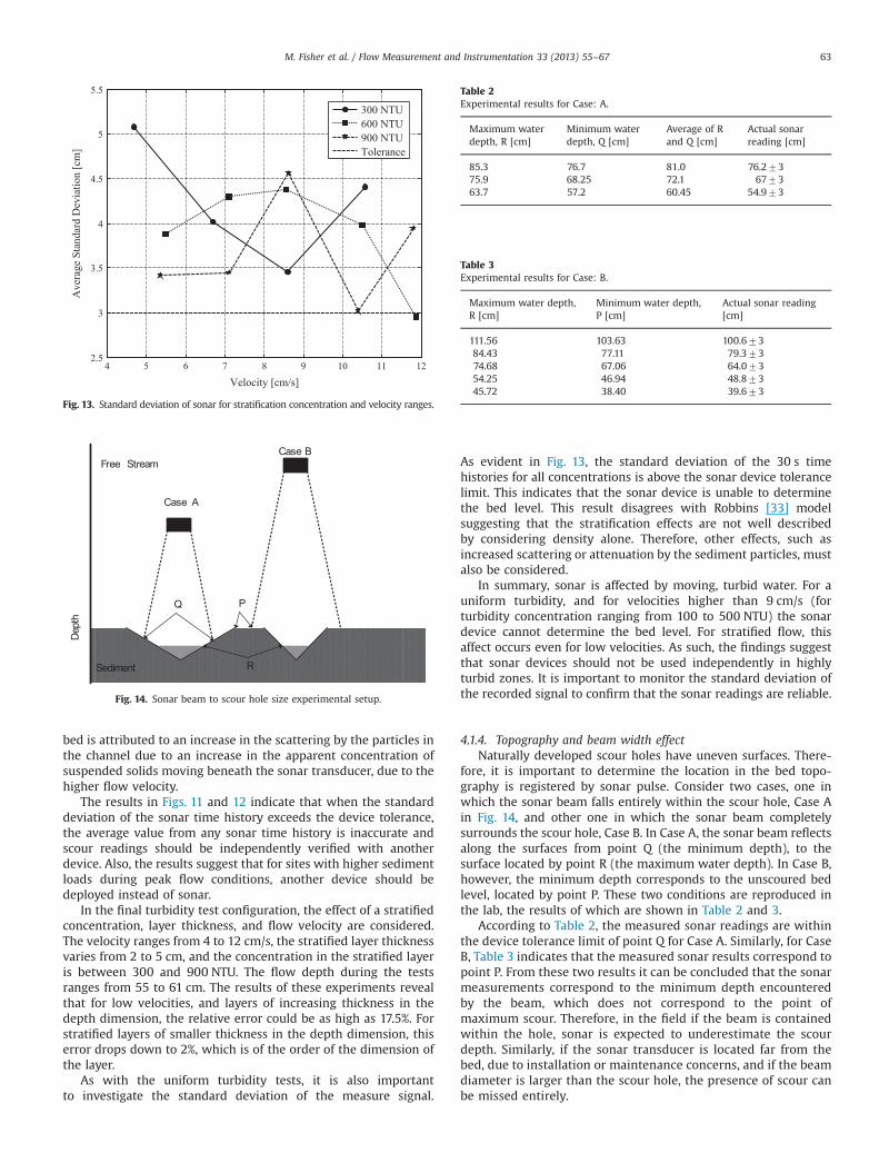
4.1.4. Topography and beam width effectNaturally developed scour holes have uneven surfaces. There-

fore, it is important to determine the location in the bed topo-graphy is registered by sonar pulse. Consider two cases, one inwhich the sonar beam falls entirely within the scour hole, Case Ain Fig. 14, and other one in which the sonar beam completelysurrounds the scour hole, Case B. In Case A, the sonar beam reflectsalong the surfaces from point Q (the minimum depth), to thesurface located by point R (the maximum water depth). In Case B,however, the minimum depth corresponds to the unscoured bedlevel, located by point P. These two conditions are reproduced inthe lab, the results of which are shown in Table 2 and 3.

According to Table 2, the measured sonar readings are withinthe device tolerance limit of point Q for Case A. Similarly, for CaseB, Table 3 indicates that the measured sonar results correspond topoint P. From these two results it can be concluded that the sonarmeasurements correspond to the minimum depth encounteredby the beam, which does not correspond to the point ofmaximum scour. Therefore, in the field if the beam is containedwithin the hole, sonar is expected to underestimate the scourdepth. Similarly, if the sonar transducer is located far from thebed, due to installation or maintenance concerns, and if the beamdiameter is larger than the scour hole, the presence of scour canbe missed entirely.

0 5 10 15 20 25 30 35 40-5

-4

-3

-2

-1

0

1

2

3

4

5

Temperature [°C]

Rel

ativ

e D

epth

Err

or [%

]

MeasuredStogryn Model

Fig. 16. Relative error in the TDR reading for various temperatures (water depth of73.5 cm).

0 5 10 15 20 25 30 35 40-5

-4

-3

-2

-1

0

1

2

3

4

55

Temperature [°C]

Rel

ativ

e D

epth

Err

or [%

]

MeasuredStogryn Model

Fig. 17. Relative error in the TDR reading for various temperatures (water depth of58.5 cm).

10 11 12 13 14 15 16 17 18

-1.2

-1

-0.8

-0.6

-0.4

-0.2

0

0.2

Apparent Length [m]

Ref

lect

ion

Coe

ffic

ient

0 PPT0.25 PPT0.50 PPT0.75 PPT

Fig. 18. Sensitivity of TDR waveform to salinity.

10 11 12 13 14 15 16 17 18-1.2

-1

-0.8

-0.6

-0.4

-0.2

0

0.2

0.4

Apparent Length [m]

Ref

lect

ion

Coe

ffic

ient

7°C12°C20°C25°C30°C35°C40°C

Increasing Temperature

A

B

Fig. 15. TDR waveform in various water temperatures for a depth 58.5 cm.

M. Fisher et al. / Flow Measurement and Instrumentation 33 (2013) 55–6764

4.2. Time domain reflectometer (TDR)

The performance of the TDR system in varying channel salinity,temperature, and turbidity are considered in the followingsections.

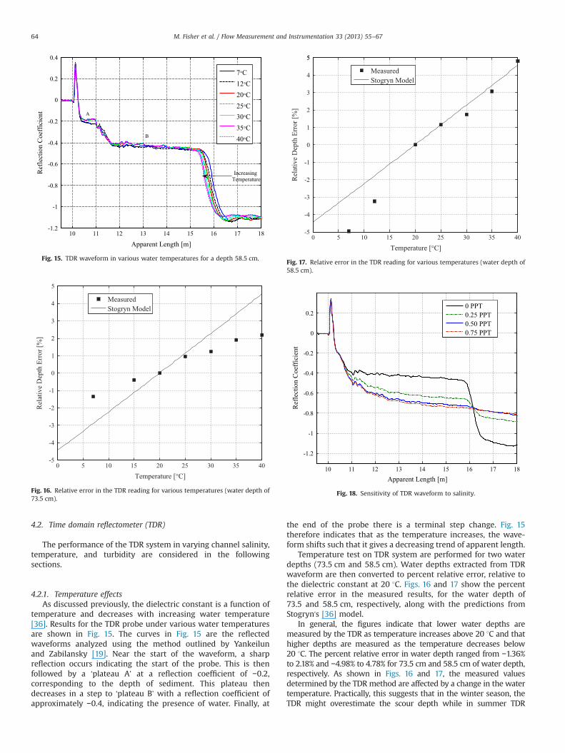
4.2.1. Temperature effectsAs discussed previously, the dielectric constant is a function of

temperature and decreases with increasing water temperature[36]. Results for the TDR probe under various water temperaturesare shown in Fig. 15. The curves in Fig. 15 are the reflectedwaveforms analyzed using the method outlined by Yankeilunand Zabilansky [19]. Near the start of the waveform, a sharpreflection occurs indicating the start of the probe. This is thenfollowed by a ‘plateau A’ at a reflection coefficient of −0.2,corresponding to the depth of sediment. This plateau thendecreases in a step to ‘plateau B’ with a reflection coefficient ofapproximately −0.4, indicating the presence of water. Finally, at

the end of the probe there is a terminal step change. Fig. 15therefore indicates that as the temperature increases, the wave-form shifts such that it gives a decreasing trend of apparent length.

Temperature test on TDR system are performed for two waterdepths (73.5 cm and 58.5 cm). Water depths extracted from TDRwaveform are then converted to percent relative error, relative tothe dielectric constant at 20 1C. Figs. 16 and 17 show the percentrelative error in the measured results, for the water depth of73.5 and 58.5 cm, respectively, along with the predictions fromStogryn's [36] model.

In general, the figures indicate that lower water depths aremeasured by the TDR as temperature increases above 20 1C and thathigher depths are measured as the temperature decreases below20 1C. The percent relative error in water depth ranged from −1.36%to 2.18% and −4.98% to 4.78% for 73.5 cm and 58.5 cm of water depth,respectively. As shown in Figs. 16 and 17, the measured valuesdetermined by the TDR method are affected by a change in the watertemperature. Practically, this suggests that in the winter season, theTDR might overestimate the scour depth while in summer TDR

0 50 100 150 200 250 300 350 400 450 500 5501

1.5

2

2.5

3

3.5

Turbidity (NTU)

Rel

ativ

e D

epth

Err

or [%

]

Fig. 19. Effect of turbidity on TDR.

0 100 200 300 400 500 600 700 800 9000

0.2

0.4

0.6

0.8

1

1.2

1.4

1.6

1.8

2x 10-3

Turbidity [NTU]

VTP

Ene

rgy

Con

tent

[m2 s-4

]

0.12 m/s0.10 m/s0.09 m/s0.07 m/s

Fig. 20. VTP energy content for various turbidity levels and channel flow velocities.

0 10 20 30 40 50 60 70 80 900

0.002

0.004

0.006

0.008

0.01

0.012

0.014

0.016

0.018

0.02

Angle From VTP Axis to Mean Flow [deg.]

VTP

Ene

rgy

Con

tent

[m2 s-

4 ]

VTP #4 - FlowVTP #5 - Scour HoleVTP #6 - Sediment

Fig. 21. VTP energy content as a function of the flow misalignment.

M. Fisher et al. / Flow Measurement and Instrumentation 33 (2013) 55–67 65

might underestimate the scour depth. The temperature dependencyof the measurements can be accounted for by measuring tempera-ture as part of the scour monitoring system.

4.2.2. Salinity effectsThe salinity of the flow can also affect the accuracy of a TDR

system [36]. Thus, TDR is tested under various salinity conditions,for which the resulting waveforms are shown in Fig. 18. The TDRwaveform, particularly the reflection at the end of the probe,becomes increasingly hard to distinguish as the salinity increases.Above 0.5 PPT, the reflection at the end of the probe is indis-tinguishable. Thus compared to the sonar, the TDR is sensitive toextremely small salinity. This degradation in performance can beattributed to the decay of the EM wave into the surroundingmedium, which becomes more conductive as the salinityincreases.

Therefore, deploying a TDR device in a saline environment or tosites that could become brackish (greater than 0.5 PPT) can lead toinconclusive results, due to the loss in the distinct features of thewaveform necessary to determine the scour depth.

4.2.3. Turbidity effectsThe results obtained for the turbidity tests conducted on the

TDR system for a water depth of 52 cm are shown in Fig. 19. Theeffect of turbidity on TDR measurements are determined bycalculating the percent relative error in water depths. For turbid-ities up to 500 NTU, the TDR system is insensitive to the presenceof suspended sediments. The offset present in the results in Fig. 19indicate the precision of the TDR device, 2.2%. The results shown inFig. 19 imply that the TDR system can be efficiently operated inhighly turbid zones.

4.3. VTP based method

As discussed in Section 2, the VTP based method has thepotential to be affected by the turbidity in the flow, as well asany misalignment between the main flow direction and the VTPaxis. The tests to evaluate the performance of the VTP deviceunder various turbidities and flow angles are discussed in thefollowing sections.

4.3.1. Turbidity effectsThe impact of dynamic turbidity on the VTP's turbulent energy

content is shown in Fig. 20 for turbidities ranging from 0 to900 NTU and flow velocities from 7 to 12 cm/s. The results indicatethat the registered energy content shows a slight increase withturbidity. The increase in the VTP energy content with flowvelocity is expected since u′ increases with the mean flow velocity.

The results shown in Fig. 20 indicate that the VTP's perfor-mance improves with the presence of turbidity in the flow, andthus can be deployed without the need to monitor the channelcondition. The energy content of the VTP buried in the bed is notaffected by turbidity and flow velocity. Therefore, the VTP methodcan reliably predict the formation of scour holes in highlyturbid zones.

4.3.2. Flow alignment effectsDuring high flow events, the main flow direction can shift from

the nominal flow condition. Therefore, it is necessary to under-stand how a VTP performs as the flow direction relative to theprobe changes. Fig. 21 shows the VTP energy content for threesensors located at different depths within the channel. VTP #6 islocated in the sediment and therefore the response should not be afunction of the flow angle as confirmed in the results shown inFig. 21. VTP #5 is located within a scour hole, for which the resultsreveal that the response is insensitive to flow angle. This is

M. Fisher et al. / Flow Measurement and Instrumentation 33 (2013) 55–6766

attributed to the fact that in the scour hole, the flow is separated.Thus, the sensor in a scour hole is subject to velocity fluctuationsfrom the separated flow instead of the turbulent free streamvelocity fluctuations. The recorded energy content for VTP #5 isan order of magnitude higher than the VTP in the bed (VTP #6),indicating that the method can be used to determine the water/sediment interface. The energy content recorded by VTP #4 issensitive to the flow angle, dropping from 0.016 m2 s−4 at 151 to0.0075 m2 s−4 at 901. This is expected as the magnitude of theturbulent fluctuations normal to the VTP surface diminishes withincreasing misalignment, while it is also important to note that theresults are still order of magnitude higher than the VTP locatedbelow the bed. The ratio between VTP #4 and VTP #6 at 901 isapproximately 75. This suggests that the method can still be usedin highly misaligned flows. For the higher flow angles, theseparated flow around the probe itself maintains the energycontent at a level much higher than the energy content in thesediment.

5. Conclusions

Given that the environmental and operational conditions innatural channels, such as temperature, salinity, and suspendedsediment change over time, it is necessary to understand howthese parameters can affect any scour monitoring system.An extensive experimental campaign is conducted on two com-mon scour measurement devices: a sonar transducer and a time-domain reflectometry probe. A novel vibration-based method,which exploits the flow turbulence in the channel, is alsoevaluated.

For the sonar device, changes in the temperature can result inrelative errors up to 6% in channel depth. The temperaturedependency can be accounted for in the field by measuring thetemperature and accounting for the change in the speed of sound.Salinity can lead to relative errors of up to 3%, which can also beaccounted for by correcting the scour measurements according tothe measured salinity levels. The concentration of suspendedparticles minimally affects the sonar results in still water. Fordynamic turbidity, uniform as well as stratified, the relative errorin bed level measurements can be significant, however. The resultsindicate that measuring the standard deviation of the recordedsignal is important to ascertain the validity of the averaged resultobtained from the sonar measurements. Lastly, for variable bedtopography, the sonar measures the shallowest depth. Therefore,the beam width at the bed with respect to scour hole maysignificantly affect the accuracy of the scour depth measurements.

For the TDR device, the channel temperature can have asignificant effect on the measured depth of a scour hole. Therelative errors can be of the order of 5%. This effect, however, canbe mitigated by monitoring the channel temperature in addition tothe TDR waveform. Salinities greater than 0.5 PPT result in a loss ofthe distinct features in the TDR waveform necessary to determinescour depth. It is recommended to only install the TDR in fresh-water conditions. Turbidity in the channel flow had no measurableeffect on the TDR measurements and thus the TDR can be used formonitoring scour in highly turbid zones.

The performance of a VTP is evaluated under turbid flowconditions and varying flow angles. There is no significant changein the energy content recorded by the VTP for varying turbidities.Thus, VTP can be successfully deployed in turbid zones. The energycontent recorded by the VTP located in the flow decreased withincreasing misalignment between the probe and the main flowdirection. Even at 901, however, the energy content of the VTP inthe flow remains an order of magnitude greater than the VTP inthe sediment. Thus, VTP can record the location of the water/

sediment interface even under significant misaligned conditionsexpected during peak flow periods.

The work presented in this manuscript has detailed potentialenvironmental and operational sensitivities of three scour mon-itoring devices by considering the physical principles behind theoperation of each device. Additionally, through a series of detailedexperiments, these sensitivities have been evaluated in order toassess the impact to scour measurements. Based upon the resultspresented, it is possible to evaluate potential scour monitoringsites and to select methods that are insensitive to the anticipatedchannel conditions, resulting in more robust field measurements.

Acknowledgments

The authors would like to thank the South Carolina Department ofTransportation for supporting this work through Grant number 1417.

References

[1] Murillo JA. The scourge of scour. Civil Engineering, ASCE 198766–69.[2] Mueller DS. National bridge scour program-measuring scour of the streambed

at highway bridges. Reston, VA: U.S. Geological Survey; 2000.[3] Lin YB, Lai JS, Chang KC, Li LS. Flood scour monitoring system using fiber Bragg

grating sensors. Smart Materials and Structures 2006;15:1950–1959.[4] Lagasse PF, Richardson EV, Schall JD, Price GR. NCHRP report 396: instrumen-

tation for measuring scour at bridge piers and abutments. TRB, NationalResearch Council, Washington D.C.; 1997

[5] Hunt D. Monitoring scour critical bridges, NCHRP synthesis 396. Washington,D.C.: Transportation Research Board; 2009.

[6] Richardson JR, Price J. Emergent techniques in scour monitoring devices. In:Shen HW, Su ST, Wen F, editors. Proceedings of the 1993 ASCE conference onhydraulic engineering. San Francisco, CA; 1993.

[7] Butch GK. Evaluation of selected instruments for monitoring scour at bridgesin New York. In: Proceedings of the North American water and environmentcongress, ASCE; 1996.

[8] Brice JC, Blodgett JC. Countermeasures for hydraulic problems at bridges, Vol. 1 & 2,FHWA/RD-78-162 & 163, Federal Highway Administration, U.S.. Washington, D.C.:Department of Transportation; 1978.

[9] Rhodes J, Trent R. Economics of floods, scour and bridge failures. In: Shen HW,Su ST, Wen F, editors. Proceedings of 1993 ASCE conference hydraulicengineering '93. San Francisco, CA; 1993.

[10] N.T.S.B. Collapse of New York Thruway (I-90) Bridge, Schoharie Creek, NearAmsterdam, New York, April 5, 1987, NTSB number: HAR-88/02, NTIS number:PB88-916202; 1987.

[11] N.T.S.B. Collapse of the Northbound U.S. Route 51 Bridge spans over theHatchie River, Near Covington, Tennessee, April 1, 1989, NTSB number: HAR-90/01, NTIS number: PB90-916201; 1987.

[12] Arneson LA, Zevenbergen LW, Lagasse PF, Clopper PE. Hydraulic EngineeringCircular no. 18: evaluating scour at bridges, 5th ed. U.S. Dept. of Transporta-tion, Federal Highway Administration, Publication no. FHWA-HIF-12-003;2012.

[13] Nassif H, Ertekin AO, Davis J. Evaluation of bridge scour monitoring methods:final report. Federal Highway Administration, Report FHWA-NJ-2003–09;March, 2002.

[14] Hunt BE. Scour monitoring programs for bridge health. TransportationResearch Record: Journal of the Transportation Research Board (WashingtonD.C.) 2005:53–536.

[15] Mason RR, Sheppard DM. Field performance of an acoustical scour-depthmonitoring system. In: Pugh CA, editor. Proceedings of the symposium onfundamentals and advancements in hydraulic measurements and experi-ments. Buffalo, N.Y. ASCE; 1994.

[16] DeFalco F, Mele R. The monitoring of bridges for scour and sedimentri. NDT&EInternational 2002;35:117–123.

[17] Holnbeck, SR, McCarthy, PM. Monitoring hydraulic conditions and scour atI-90 Bridges on Blackfoot River following removal of Milltown Dam nearBonner, Montana, 2009. In: Burns SE, Bhatia SK, Avila CMC, Hunt BE, editors.Proceedings of 5th international conference on scour and erosion. SanFrancisco, CA, ASCE; 2010.

[18] Cooper T, Chen HL, Lyn D, Rao AR, Altschaeffel AG. A field study of scour-monitoring devices for indiana streams: final report, FHWA/IN/JTRP-2000/13;October, 2000.

[19] Yankielun NE, Zabilansky L. Laboratory investigation of time domain reflecto-metry system for monitoring bridge scour. Journal of Hydraulic Engineering,ASCE 1999;125(12):1279–1284.

[20] Yu X, Yu X. Time domain reflectometry tests of multilayered soils. In:Proceedings of the TDR 2006. Purdue University: West Lafayette, U.S.A.; 2006.

[21] Yu X, Yu X. Development and evaluation of an automatic algorithm for a time-domain reflectometry bridge scour monitoring system. Canadian GeotechnicalJournal 2011;48:26–35.

M. Fisher et al. / Flow Measurement and Instrumentation 33 (2013) 55–67 67

[22] Yu X, Zabilansky LJ. Time domain reflectometry for automatic bridge scourmonitoring. In: Puppala AJ, Fratta D, Alshibli K, Pamukcu S, editors. GeoShan-ghai 2006: Site and Geomaterial Characterization, GSP 149. Reston, Virginia,USA: ASCE; 2006.

[23] Ettema R, Zabilansk L. Ice influences on channel stability: insights fromMissouri's Fort Peck Reach. Journal of Hydraulic Engineering, ASCE 2004;130(4):279–292.

[24] Zabilansky, L, Ettema, R, Weubeen, J, Yankielun, N. Survey of river iceinfluences on channel bathymetry along the Fort Peck Reach of the MissouriRiver, Winter 1998–1999, Technical report ERDC/CRREL TR-02-14, U.S. ArmyCorps of Engineers, Engineer Research and Development Center; September,2002.

[25] USGS. Water Data report 2006: 02172053 Cooper River at Mobay near NorthCharleston, S.C., U.S. Department of Interior, U.S. Geological Survey; 2006.

[26] USGS. Water Data report 2006: 02156500 Broad River Near Carlisle, S.C., U.S.Department of Interior, U.S. Geological Survey; 2006.

[27] Fisher M, Atamturktur S, Khan AA. A novel vibration-based monitoringtechnique for bridge pier and abutment scour. Journal of Structural HealthMonitoring 2013;12(2):114–125.

[28] Kuwahara S. Velocity of sound in sea water and calculations of the velocity foruse in sonic soundings. Hydrogeologic Reviews 1939;16:123–140.

[29] Leroy CC. Development of simple equations for accurate and more realisticcalculation of the speed of sound in seawater. Journal of the Acoustical Societyof America 1969;46(1B).

[30] Urick RJ. Principles of underwater sound. New York, USA: McGraw-Hill Inc;1975.

[31] MacKenzie KV. Nine‐term equation for sound speed in the oceans. Journal ofthe Acoustical Society of America 1981;70(3):807–812.

[32] Hamilton EL. Geoacoustical modeling of the sea floor. Journal of the AcousticalSociety of America 1980;68(5):1313–1340.

[33] Robins AJ. Reflection of plane acoustic waves from a layer of varying density.Journal of the Acoustical Society of America 1990;87(4):1546–1552.

[34] Stoll RD, Kan T-K. Reflection of acoustic waves at a water–sediment interface.Journal of the Acoustical Society of America 1981;70(1):149–156.

[35] Gray JR, Melis TS, Patiño E, Larsen MC, Topping DJ, Rasmussen PP, et al. USGeological Survey Research on surrogate measurements for suspended sedi-ment. In: Proceedings of the 1st interagency conference on research inwatersheds; 2003. p. 95–100.

[36] Stogryn A. Equations for calculating the dielectric constant of saline water.IEEE Transactions on Microwave Theory and Techniques 1971:733–736.

[37] Das BM. Principles of geotechnical engineering. 4th Ed. Boston, MA: PWSPublishing Company; 1998.

[38] Itakura T, Kishi T. Open channel flow with suspended sediments. Journal of theHydraulics Division, Proceedings of the American Society of Civil Engineers, ASCE1980;106(HY8):1325–1343.

[39] Coleman NL. Velocity profiles with suspended sediment. Journal of HydraulicResearch 1981;19(3):211–229.

[40] Nezu I, Azuma R. Turbulence characteristics and interaction between particles andfluid in particle-laden open channel flows. Journal of Hydraulic Engineering, ASCE2004;130(10):988–1001.

[41] Dey S, Raikar RV. Characteristics of loose rough boundary streams at near-threshold. Journal of Hydraulic Engineering, ASCE, 133; 228–304.

[42] Nikora V, Goring D. Flow turbulence over fixed and weakly mobile gravel beds.Journal of Hydraulic Engineering, ASCE, 126; 679–690.

[43] Henderson FM. Open channel flow. Upper Saddle River, NJ: Prentice Hall Inc.;1966.