Scour and scour protection around offshore gravity based ...

1

UCL

Scour and scour protection around offshore gravity based foundations Eng D in Urban Sustainability and Resilience

Mr Nikolas Sokratis Tavouktsoglou

2

l, Nikolas Sokratis Tavouktsoglou confirm that the work presented in this thesis is my own. Where information has been derived from other sources, confirm that this has been indicated in the thesis. Signed,

Nikolas Sokratis Tavouktsoglou

------------------------------------------------

3

Abstract

The prediction of seabed scour around offshore gravity based foundations with complex

geometries is currently a significant barrier to optimising and providing cost effective

foundation designs. A significant aspect that has the potential to reduce the uncertainty

and costs related to the design of these foundations is the understanding of the effect

the structural geometry of the foundation has on scour.

This thesis focuses on an experimental investigation of the scour and scour protection

around complex structure geometries. The first part of this research considers scour

under clear water conditions. During this study different foundation geometries were

subjected to a range of different hydrodynamic forcings which enabled a better

understanding of the scour process for these foundations. The second part of the

research encompasses the design and execution of a series of experiments which

investigated stability of the scour protection around such structures. The structures were

tested against different combinations of wave and current conditions to determine the

bed shear stress required to initiate sediment motion around each structure.

This research has led to a number of novel results. The experimental investigation on

scour around complex geometries showed that the scour depth around cylindrical

structures (with both uniform and complex cross-sections) is linked to the depth averaged

pressure gradient. Following a dimensional analysis, the controlling parameters were

found to be the depth averaged Euler number, pile Reynolds number, Froude number,

sediment mobility number and the non-dimensional flow depth. Based on this finding a

new scour prediction equation was developed which shows good agreement with

experimental and prototype scour measurements. The scour protection tests indicated

that under wave dominated conditions the amplification of the bed shear stress around

these structures does not exceed the value of 2. In the case of current dominated flow

conditions the amplification of the bed shear stress is a function of the structure type and

the Keulegan–Carpenter number. The results of these experiments were used to develop

4

a “Shields type” diagram that can guide designers to select the appropriate rock armour

size that will be stable for a certain set of flow conditions. The study also revealed that

the long term persistence of flow conditions that just lead to incipient motion of the scour

protection material can eventually lead to complete failure of the scour protection.

The study provides a set of new design techniques that can allow designers to predict

the scour depth around cylindrical and complex foundation geometries and also select

the appropriate stone size for their scour protection system. Together, these techniques

may allow for the reduction of costs associated with the scour protection of offshore and

coastal structures.

5

Table of Contents

Abstract ....................................................................................................................... 3

Table of Contents ....................................................................................................... 5

List of Figures ........................................................................................................... 13

List of Tables ............................................................................................................ 24

Nomenclature ............................................................................................................ 25

List of publications ................................................................................................... 33

Acknowledgments .................................................................................................... 34

Part I: Overview of scour and scour

protection around complex foundations

1 Introduction ........................................................................................................ 35

1.1 General overview of the research ............................................................................... 35

1.2 Background ................................................................................................................. 35

1.3 Thesis outline .............................................................................................................. 37

2 Literature review ................................................................................................ 38

2.1 Introduction .................................................................................................................. 38

2.2 Sediment transport and boundary layer theory ........................................................... 38

2.2.1 Steady uniform flow ............................................................................................. 40

2.2.2 Wave boundary layer .......................................................................................... 42

2.2.3 Wave current interaction ..................................................................................... 44

2.2.3.1 Wavelength modification ................................................................................. 44

6

2.2.3.2 Wave current boundary layer ........................................................................... 45

2.2.4 Incipient motion of sediment particles ................................................................. 47

2.2.5 Threshold current speed ...................................................................................... 54

2.3 Hydrodynamics around cylindrical structures .............................................................. 54

2.3.1 Downflow ............................................................................................................. 56

2.3.2 Horseshoe vortex ................................................................................................. 57

2.3.2.1 Horseshoe vortex in currents ........................................................................... 57

2.3.2.2 Horseshoe vortex in waves .............................................................................. 61

2.3.2.3 Horseshoe vortex in combined waves and currents ........................................ 62

2.3.3 Lee-wake vortex................................................................................................... 64

2.3.3.1 Lee-wake vortex in currents ............................................................................. 64

2.3.3.2 Lee-wake vortex in waves ............................................................................... 67

2.3.4 Streamline contraction ......................................................................................... 70

2.4 Scour around cylindrical structures ............................................................................. 70

2.4.1 Scour types .......................................................................................................... 70

2.4.1.1 General (global) scour ..................................................................................... 71

2.4.1.2 Local scour ....................................................................................................... 72

2.4.2 Sediment transport in local scour ........................................................................ 73

2.4.3 Scour in steady unidirectional currents ................................................................ 75

2.4.3.1 Influencing parameters .................................................................................... 76

2.4.3.1.1 Sediment mobility ratio .............................................................................. 77

2.4.3.1.2 Relative flow depth .................................................................................... 79

2.4.3.1.3 Sediment gradation .................................................................................... 81

2.4.3.2 Time evolution of scour .................................................................................... 81

2.4.3.3 Equilibrium scour depth prediction................................................................... 83

2.4.4 Scour under wave action ..................................................................................... 86


2.4.4.2 Time evolution of scour .................................................................................... 87

2.4.4.3 Equilibrium scour prediction ............................................................................. 87

2.4.5 Scour under the forcing of combined waves and currents .................................. 89

7


2.4.5.2 Time evolution of scour ................................................................................... 90

2.4.5.3 Equilibrium scour depth prediction .................................................................. 91

2.5 Scour around gravity based foundation ...................................................................... 92

2.5.1 Introduction .......................................................................................................... 92

2.5.2 Scour in steady unidirectional currents ............................................................... 93


2.5.2.2 Time evolution of scour ................................................................................... 94

2.5.2.3 Equilibrium scour depth prediction .................................................................. 95

2.5.3 Scour under wave action ..................................................................................... 98

2.5.4 Scour under combined wave and current action ................................................. 99

2.5.5 Discussion on scour prediction around GBFs ................................................... 100

2.6 Scour protection practice .......................................................................................... 100

2.6.1 Introduction ........................................................................................................ 100

2.6.2 Armour layer ...................................................................................................... 102

2.6.2.1 Stone size ...................................................................................................... 102

2.6.2.2 Thickness ...................................................................................................... 106

2.6.2.3 Lateral extent ................................................................................................. 107

2.6.3 Granular filter layer ............................................................................................ 108

2.6.3.1 Geometrically closed filters ........................................................................... 108

2.6.3.2 Geometrically open filters .............................................................................. 109

2.6.4 Discussion on scour protection practice ........................................................... 110

3 Aims and objectives ........................................................................................ 112

Part II: Scour around complex foundations

4 Methodology .................................................................................................... 115

4.1 Introduction ................................................................................................................ 115

4.2 General model and scaling considerations ............................................................... 116

8

4.2.1 Scaling considerations ....................................................................................... 116

4.2.1.1 Hydrodynamic scaling .................................................................................... 116

4.2.1.2 Sediment scaling ........................................................................................... 117

4.2.2 Model effects...................................................................................................... 119

4.3 Description of set-up and the models for small scale scour tests ............................. 120

4.3.1 Flume and test set-up ........................................................................................ 120

4.3.1.1 Sand installation and smoothing .................................................................... 122

4.3.1.2 Model Structures ............................................................................................ 122

4.3.2 Flow parameters ................................................................................................ 124

4.3.2.1 Flow velocity .................................................................................................. 124

4.3.2.2 Flow depth ..................................................................................................... 125

4.3.2.3 Sediment characteristics ................................................................................ 125

4.3.3 Measurement techniques .................................................................................. 126

4.3.3.1 Flow velocity measurements ......................................................................... 126

4.3.3.2 Flow and scour depth measurements ........................................................... 129

4.3.4 Experimental programme .................................................................................. 130

4.4 Description of set-up and the models for large scale scour experiments .................. 132


4.4.2 Flow parameters ................................................................................................ 136

4.4.3 Measuring techniques ........................................................................................ 137

4.4.3.1 Flow velocity measurement ........................................................................... 137

4.4.3.2 Flow and water depth measurement ............................................................. 138

4.4.4 Experiment programme ..................................................................................... 139

4.5 Description of set-up and the models for the pressure and flow measurements near

the structure ........................................................................................................................... 141


4.5.2 Measurement techniques .................................................................................. 145

4.5.2.1 Pressure measurement ................................................................................. 145

4.5.3 Experimental programme .................................................................................. 146

4.6 Database compilation for equilibrium scour prediction equation ............................... 147

9

5 Results for scour around complex structures ............................................... 149

5.1 Smaller scale scour results ....................................................................................... 149

5.1.1 Flow conditions .................................................................................................. 149

5.1.2 Results .............................................................................................................. 150

5.1.2.1 Initiation of scour around complex geometries ............................................. 150

5.1.2.2 Temporal evolution of scour .......................................................................... 151

5.1.2.3 Equilibrium scour depth ................................................................................. 159

5.1.2.4 Repeatability of tests ..................................................................................... 162

5.2 Large scale scour results .......................................................................................... 165

5.2.1 Flow conditions .................................................................................................. 165

5.2.2 Results .............................................................................................................. 167

5.2.2.1 Temporal evolution of scour .......................................................................... 167

5.2.2.2 Equilibrium scour depths ............................................................................... 171

5.2.2.3 Repeatability of tests ..................................................................................... 178

5.3 Pressure and flow measurement .............................................................................. 179

5.3.1 Test conditions .................................................................................................. 180

5.3.2 Pressure Measurements ................................................................................... 180

5.3.3 Flow measurements .......................................................................................... 185

5.3.3.1 Monopile ........................................................................................................ 185

5.3.3.2 75⁰ conical base structure ............................................................................. 188

5.3.3.3 60⁰ conical base structure ............................................................................. 191

5.3.3.4 Cylindrical base ............................................................................................. 192

5.4 Summary of results ................................................................................................... 194

6 Prediction of equilibrium scour depth around cylindrical structures .......... 197

6.1 Introduction ................................................................................................................ 197

6.2 Similitude of scour at complex geometries ............................................................... 197

6.3 Database Description ................................................................................................ 205

6.4 Equilibrium scour depth prediction equation ............................................................. 208

10

6.5 Behaviour of scour prediction equation ..................................................................... 217

6.5.1 Influence of depth averaged Euler number ....................................................... 217

6.5.2 Influence of pile Reynolds number .................................................................... 221

6.5.3 Influence of Froude number ............................................................................... 224

6.5.4 Influence of non-dimensional flow depth ........................................................... 226

6.5.5 Influence of the sediment mobility ratio ............................................................. 228

Part III: Scour protection around complex

foundations

7 Methodology for scour protection stability tests .......................................... 230

7.1 Introduction ................................................................................................................ 230

7.2 General model and scaling considerations ................................................................ 230

7.3 Experimental procedure ............................................................................................. 231

7.4 Description of flume and the models ......................................................................... 233

7.5 Flow parameters ........................................................................................................ 238

7.6 Measuring techniques ................................................................................................ 240

7.6.1 Detection of incipient motion for scour protection.............................................. 240

7.6.2 Flow velocity measurement ............................................................................... 242

7.6.3 Measurement of scour protection damage ........................................................ 243

7.6.4 Wave measurements ......................................................................................... 244

7.7 Experiment programme ............................................................................................. 244

8 Results for scour protection around complex structures ............................. 257

8.1 Flow characteristics ................................................................................................... 257

8.2 Stability of scour protection........................................................................................ 260

8.2.1 Choice of wave friction formula.......................................................................... 260

8.3 Analysis of the results of scour protection stability tests ........................................... 262

11

8.3.1 Influence of main variables ............................................................................... 263

8.3.1.1 Influence of stone size (𝑫𝟓𝟎) ....................................................................... 263

8.3.1.2 Influence of scour protection level................................................................. 264

8.3.1.3 Influence of bed permeability ........................................................................ 265

8.3.1.4 Influence of flow direction .............................................................................. 266

8.3.1.5 Influence of wavelength ................................................................................ 267

8.3.1.6 Influence of the velocity ratio (𝑼𝒄𝒘) ............................................................. 268

8.3.1.7 Influence of the KC number: Design diagram for rock cover size selection . 269

8.3.2 Validation of present results .............................................................................. 274

8.4 Development of scour protection damage ................................................................ 275

8.4.1 Monopile damage pattern ................................................................................. 276

8.4.2 75⁰ conical base ................................................................................................ 279

8.4.3 45⁰ conical base ................................................................................................ 282

8.4.4 Cylindrical base structure .................................................................................. 284

8.4.5 Discussion of results ......................................................................................... 286

Part IV: Conclusions and recommendations

9 Conclusions and recommendations .............................................................. 287

9.1 Conclusions ............................................................................................................... 287

9.2 Recommendations .................................................................................................... 290

10 References .................................................................................................... 292

Part V: Appendices

11 Appendix A (correction factors for scour prediction equations) .............. 312

11.1.1 Sediment gradation (𝑲𝝈) .................................................................................. 312

11.1.2 Foundation shape factor (𝑲𝒔) ........................................................................... 313

11.1.3 Pier orientation factor (𝑲𝝎) .............................................................................. 314

11.1.4 Pier group factor (𝑲𝒈𝒓) ..................................................................................... 315

12

12 Appendix B (scour profiles along the centreline of the structures) ......... 318

13

List of Figures

Figure 1-1: Breakdown of costs for offshore wind turbines. [Data derived from Blanco

(2009)]. ....................................................................................................................... 36

Figure 2-1: Boundary layer definition sketch ............................................................... 40

Figure 2-2: Definition sketch and zones of turbulence (proposed by Lundgren, 1971). 46

Figure 2-3: Definition sketch of forces acting on a single sediment particle. ................ 47

Figure 2-4: Original Shields curve (Shields, 1936) ...................................................... 50

Figure 2-5: Modified Shields diagram (Miller et al., 1977) ........................................... 52

Figure 2-6: Updated Shields diagram (Source: Soulsby, 1997) ................................... 52

Figure 2-7: Sundborg’s modification of the Hjulström diagram. (After Sundborg, 1956.)

................................................................................................................................... 53

Figure 2-8: Flow structure interaction definition sketch (source: Roulund et al., 2005) 55

Figure 2-9: Definition sketch of downflow phenomenon (location of the stagnation point

is arbitrarily selected in this image) ............................................................................. 56

Figure 2-10: Influence of the 𝑅𝑒𝐷 on the Horseshoe vortex (source: Roulund et al., 2005)

................................................................................................................................... 58

Figure 2-11: Influence of the boundary layer thickness on the Horseshoe vortex for

𝑅𝑒𝐷 = 2 ∗ 102, line: result of numerical model, x symbol: experimental measurement

(source: Roulund et al., 2005). .................................................................................... 59

Figure 2-12: Boundary layer separation distance for different cross-sectional shapes

(source: Sumer et al., 1997) ....................................................................................... 60

Figure 2-13: Horseshoe vortex in different phases of wave cycle (Source: Sumer et al.,

1997) .......................................................................................................................... 62

Figure 2-14: Presence of horseshoe vortex in phase space: influence of superimposed

current (Source: Sumer et al., 1997) ........................................................................... 63

Figure 2-15:SepaType equation here.ration distance for combined waves and currents

(Source: Umeda et al., 2003) ...................................................................................... 64

14

Figure 2-16: Lee wake vortex shedding regimes around a cylinder (source: Sumer and

Fredsøe, 1997) ........................................................................................................... 65

Figure 2-17: Strouhal number as a function of the pile Reynolds number for smooth and

rough cylinders (Data source: Roshko, 1961) ............................................................. 66

Figure 2-18: Effect of cross-flow shape on the Strouhal number (Source: Blevins and

Burton, 1976) .............................................................................................................. 66

Figure 2-19: Regimes of flow separation around cylinders in waves (source: Sumer and

Fredsøe, 1997) ........................................................................................................... 67

Figure 2-20: Flow separation regimes for small 𝐾𝐶 and very small 𝑅𝑒𝐷 numbers (source:

Sumer and Fredsøe, 1997) ......................................................................................... 68

Figure 2-21: Flow separation regimes for large 𝐾𝐶 and 𝑅𝑒𝐷 numbers (source: Sumer

and Fredsøe, 1997) .................................................................................................... 68

Figure 2-22: Definition sketch of steady streaming ...................................................... 69

Figure 2-23: Size of steady streaming cell (Reproduced from Wang, 1968) ................ 69

Figure 2-24: Definition sketch of local scour around monopile in unidirectional flow. ... 71

Figure 2-25: Scour depth evolution, live bed Vs clear water scour. ............................. 73

Figure 2-26: Development of clear-water scour (Derived from: Hoffmans and Verheij,

1997) .......................................................................................................................... 74

Figure 2-27: Counter-rotating streamwise phase-averaged vortices (a) streamlines (b)

mean vorticity in x- direction (Source: Baykal et al., 2015) .......................................... 77

Figure 2-28: Influence of flow intensity on scour depth (Derived from: Melville and

Sutherland, 1988) ....................................................................................................... 79

Figure 2-29: Effect of flow shallowness on scour depth (Source: Melville, 2008) ......... 80

Figure 2-30: Examples of GBF foundation geometries. ............................................... 92

Figure 2-31: Definition sketch of key structural parameters of composite cylindrical

structures. ................................................................................................................... 94

Figure 2-32: Definition diagram of scour protection design. ....................................... 102

Figure 2-33:Types of filters. ...................................................................................... 108

15

Figure 4-1: Layout of tidal flume: (a) top view; (b) side view. ..................................... 121

Figure 4-2: Structure geometries for scour tests. ...................................................... 123

Figure 4-3: Set-up of the structures for scour tests: (a) Lower part of model (buried under

the sand); (b) installation of model foundation on base. ............................................ 124

Figure 4-4: Grain size distribution for the two sediment types used in the experiments.

................................................................................................................................. 126

Figure 4-5: Schematic of LDV working principle ........................................................ 127

Figure 4-6: Traverse set-up with LDV ....................................................................... 128

Figure 4-7: Flow velocity in the cross-flow direction. ................................................. 129

Figure 4-8: Layout of costal flume in Mechanical Engineering Department ............... 134

Figure 4-9: Image of the flow conditioner. ................................................................. 135

Figure 4-10: Large scale foundation geometries ....................................................... 135

Figure 4-11: Schematic of the flow profiles tested in these tests. .............................. 136

Figure 4-12: Acoustic Doppler Velocimetry working principle (source: Sellar et al., 2015).

................................................................................................................................. 138

Figure 4-13: (a) Set up of the pressure measurement tests showing the acrylic tubes

connecting to the pressure transducer units beneath the flume; (b) Image of 3D model;

(c) cut through (from centreline) of model with tubes. ............................................... 142

Figure 4-14: Location of pressure taps. ..................................................................... 142

Figure 4-15: Side view sketch of the lower part of the pressure measurement apparatus.

................................................................................................................................. 143

Figure 4-16: Flow field measurement points in the X-Y plane. .................................. 144

Figure 4-17: Flow field measurement points in the X-Z plane.................................... 144

Figure 4-18: Pressure transducer ............................................................................. 145

Figure 5-1: Flow profiles for small scale scour tests: a) h=165mm and b) h=100mm. 150

Figure 5-2: (a) Initiation of scour at 45° conical base structure, (b) bed shear stress

amplification contour map for same structure; flow direction from left to right. ........... 151

16

Figure 5-3: Time development of scour for tests 1.0-1.5 (ℎ = 0.165𝑚, 𝑑50 =

0.6𝑚𝑚 𝑎𝑛𝑑 𝑈𝑐/𝑈𝑐𝑟 = 0.73). ...................................................................................... 152


0.2𝑚𝑚 𝑎𝑛𝑑 𝑈𝑐/𝑈𝑐𝑟 = 0.88). ...................................................................................... 153


0.2𝑚𝑚 𝑎𝑛𝑑 𝑈𝑐/𝑈𝑐𝑟 = 0.98). ...................................................................................... 154


0.6𝑚𝑚 𝑎𝑛𝑑 𝑈𝑐/𝑈𝑐𝑟 = 0.88). ...................................................................................... 155


0.6𝑚𝑚 𝑎𝑛𝑑 𝑈𝑐/𝑈𝑐𝑟 = 0.99). ...................................................................................... 155

Figure 5-8: Time development of scour for tests 2.1-2.6 (ℎ = 0.1𝑚, 𝑑50 = 0.2𝑚𝑚 𝑎𝑛𝑑 𝑈𝑐/

𝑈𝑐𝑟 = 0.93). .............................................................................................................. 156


0.6𝑚𝑚 𝑎𝑛𝑑 𝑈𝑐/𝑈𝑐𝑟 = 0.78). ...................................................................................... 157

Figure 5-10: Influence of 𝑈𝑐/𝑈𝑐𝑟 on scour development for three different structure

geometries. ............................................................................................................... 158

Figure 5-11: Observed scour depth at cylindrical based pier before under-cutting the

base cylinder (ℎ = 0.165𝑚, 𝑑50 = 0.6𝑚𝑚 𝑎𝑛𝑑 𝑈𝑐/𝑈𝑐𝑟 = 0.88). ................................. 159

Figure 5-12: Influence of water depth on equilibrium scour depth for different structure

types (non-dimensionalised by base diameter of the structure). ................................ 162

Figure 5-13: Influence of water depth on equilibrium scour depth for different structure

types (non-dimensionalised by equivalent diameter according to Coleman, 2005). ... 162

Figure 5-14: Comparison of test 1.5 with Porter (2016) with D=40mm, 𝑈𝑐 = 0.19𝑚/𝑠 and

𝑑50 = 0.6𝑚𝑚. ........................................................................................................... 164

Figure 5-15: Comparison of test 1.11 with Porter (2016) with D=40mm, 𝑈𝑐 = 0.19𝑚/𝑠

and 𝑑50 = 0.2𝑚𝑚 . ................................................................................................... 164

Figure 5-16: Flow profiles for large scale scour tests: a) logarithmic flow profile and b)

non-logarithmic flow profiles. ..................................................................................... 166

17

Figure 5-17: Velocity profiles when the wind is opposing the tide (left) and when the wind

is following the tide (Source: Holmedal and Myrhaug, 2013). .................................... 166

Figure 5-18: Temporal evolution of scour for a logarithmic flow profile, h=350mm. ... 168

Figure 5-19: Temporal evolution of scour for non-logarithmic flow profile, h=350mm 169

Figure 5-20: Temporal evolution of scour for non-logarithmic flow profile, h=550mm.170

Figure 5-21: Temporal evolution of scour for the 75deg conical base structure with non-

logarithmic flow profile, h=350mm, h=450mm and h=550mm. .................................. 170

Figure 5-22: Equilibrium scour depth profiles for Tests 3-1-3.4 at h=350mm and a

logarithmic flow profile (flow from bottom): a) Monopile; b) Cylindrical base; c) 45⁰ conical

base structure; and d) 75⁰ conical base structure. .................................................... 172

Figure 5-23: Equilibrium scour depth profiles for Tests 3-5-3.8 at h=350mm and a non-

logarithmic flow profile (flow from bottom to up): a) Monopile; b) Cylindrical base; c) 45⁰

conical base structure; and d) 75⁰ conical base structure. ......................................... 174

Figure 5-24: Equilibrium scour depth profiles for Tests 3-9-3.12 at h=550mm and a non-

logarithmic flow profile (flow from bottom to up): a)Monopile; b)Cylindrical base; c) 45⁰

conical base structure; and d) 75⁰ conical base structure. ......................................... 176

Figure 5-25: Equilibrium scour depth profiles 75⁰ conical base structure at three different

flow depths and a non-logarithmic flow profile (Tests 3-12-3.14): a) h=550mm; b)

h=450mm; and c) h=350mm. .................................................................................... 177

Figure 5-26: Comparison of time development of Test 3.8 and 3.14. ........................ 178

Figure 5-27: Comparison of scour contour maps between tests 3.14 and 3.8: a) Test

3.14; b) test 3.8; and c) the difference between 3.8 and 3.14. ................................... 179

Figure 5-28: Flow profile for tests 4.1-4.5. ................................................................. 180

Figure 5-29: Pressure variation for the cylindrical base structure. ............................. 182

Figure 5-30: Pressure variation for the 45⁰ conical base structure. ........................... 183

Figure 5-31: Pressure variation for the 60⁰ conical base structure. ............................ 183

Figure 5-32: Pressure variation for the 75⁰ conical base structure. ............................ 184

Figure 5-33: Pressure variation for the monopile structure. ....................................... 185

18

Figure 5-34: Vertical velocity component (w) distribution and u-w velocity vectors along

the centreline of the monopile. .................................................................................. 186

Figure 5-35: Contours of streamwise velocity component (u) around the monopile at

different heights. ....................................................................................................... 187

Figure 5-36: Contours of vertical velocity component (w) around the monopile at different

heights. ..................................................................................................................... 188


the centreline of the 75⁰ conical base structure. ........................................................ 189

Figure 5-38: Contours of streamwise velocity component (u) around the 75⁰ conical base

structure. at different heights. .................................................................................... 190

Figure 5-39: Contours of vertical velocity component (w) around the 75⁰ conical base

structure. at different heights. .................................................................................... 191


the centreline of the 60⁰ conical base structure. ........................................................ 191


the centreline of the cylindrical base structure. .......................................................... 192

Figure 5-42: Contours of streamwise velocity component (u) around the cylindrical base

structure at different heights. ..................................................................................... 193

Figure 5-43: Contours of vertical velocity component (w) around the cylindrical base

structure at different heights. ..................................................................................... 194

Figure 6-1: Definition sketch of main parameters: (a) side view; (b) top view. ........... 198

Figure 6-2: Pressure gradient distribution through the water column [calculated using Eq.

(6-8)] for two different structures under the same flow conditions. ............................. 204

Figure 6-3: Percentage distribution of non-dimensional quantities in database ......... 206

Figure 6-4: Scour depth as a function of ℎ/𝐷𝑏𝑎𝑠𝑒 . .................................................. 210

Figure 6-5: Scour depth as a function of ℎ/𝐷𝑏𝑎𝑠𝑒 𝐹𝑟 .............................................. 211

Figure 6-6: Scour depth as a function of ℎ/𝐷𝑏𝑎𝑠𝑒 𝐹𝑟 1/𝑙𝑜𝑔 (𝑅𝑒𝐷) . ........................... 212

Figure 6-7: Scour depth as a function of ℎ/𝐷𝑏𝑎𝑠𝑒 𝐹𝑟 1/𝑙𝑜𝑔𝑅𝑒𝐷(𝑈𝑐/𝑈𝑐𝑟)0.5 . ........... 212

19

Figure 6-8: Scour depth as a function of ζ. ................................................................ 214

Figure 6-9: Agreement of scour-depth prediction [using Equation (6-17)] and measured

scour depths with 10 and 20% confidence bounds ................................................... 216

Figure 6-10: Comparison of Equation (6-17) with prototype field data. ...................... 217

Figure 6-11: Influence of sediment mobility ratio [𝑈𝑐/𝑈𝑐𝑟 =0.74, 0.88 and 1] on the

variation of the equilibrium scour depth as a function of < 𝐸𝑢 > [Note: Line shows

prediction given by Equation (6-17) for each of the three sediment mobility ratios. ... 219

Figure 6-12: Influence of non-dimensional water depth [ℎ/𝐷𝑏𝑎𝑠𝑒 =3.6 and 2.2] on the

variation of the equilibrium scour depth as a function of < 𝐸𝑢 > [Note: Line shows

prediction given by Equation (6-17) for each of the three sediment mobility ratios. ... 219

Figure 6-13: Influence of vertical flow distribution on the variation of the equilibrium scour

depth as a function of < 𝐸𝑢 > [Note: solid line shows prediction given by Equation (6-17)]

................................................................................................................................. 220

Figure 6-14: Influence of 𝑅𝑒𝐷 on equilibrium scour. Comparison of Equation (6-17) to

scour depth data with varying 𝑅𝑒𝐷 and 𝐹𝑟 = {0.15 − 0.20}, 𝑈𝑐/𝑈𝑐𝑟 = {0.7 − 0.85}, ℎ/𝐷 =

{2 − 3} 𝑎𝑛𝑑 ⟨𝐸𝑢⟩ = {1.7 − 2} (data from dataset collected from current study). ......... 222

Figure 6-15: Effect of the pile Reynolds number on scour. Comparison of present

equation (Equation (6-17)) and the equation of Shen et al, (1969) [Equation 2-54] to the

data presented in Breusers et al. (1977) (data source: Sheppard et al., 2011). ......... 224

Figure 6-16: Definition diagram of the location of the vertical stagnation point. ......... 225

Figure 6-17: Influence of Fr on equilibrium scour. Comparison of Equation (6-17)) to

scour depth data with varying 𝐹𝑟 and 𝑅𝑒𝐷 = {75000 − 150000},𝑈𝑐/𝑈𝑐𝑟 = {0.8 −

1}, ℎ/𝐷 = {2 − 3} ⟨𝐸𝑢⟩ = {1.7 − 2}. ............................................................................ 226

Figure 6-18: Influence of h/D on equilibrium scour. Comparison of Equation (6-17) to

scour depth data with varying h/D and 𝑅𝑒𝐷 = 100000 − 300000,𝑈𝑐/𝑈𝑐𝑟 = {0.8 −

1}, 𝐹𝑟 = {0.1 − 0.25} and 𝐸𝑢 = {1.7 − 2}. .................................................................. 227

Figure 6-19: Effect of boundary layer thickness on scour. Comparison of Equation (6-17)

with clearwater scour data compiled from Melville and Sutherland (1988). ............... 228

20

Figure 6-20: Effect of sediment mobility ratio on scour for monopiles. Comparison of

Equation (6-17) to scour depth data with varying 𝑈𝑐/𝑈𝑐𝑟𝑎𝑛𝑑 𝑅𝑒𝐷 = 50000 −

200000, ℎ/𝐷 = 3 − 6, 𝐹𝑟 = 0.1 − 0.15 𝑎𝑛𝑑 𝐸𝑢 = {1.7 − 2}. ......................................... 229

Figure 7-1: Wave absorber reflection vs incoming wave period ( Figure derived from:

Edinburgh Designs Ltd, 2005) ................................................................................... 231

Figure 7-2: Flow chart of experimental procedure. .................................................... 233

Figure 7-3: Positions of wave probes (red lines indicate position of the wave probes).

................................................................................................................................. 234

Figure 7-4: Layout of scour protection set-up for present tests. ................................. 234

Figure 7-5: U-pins used to provide stability to the fabric. ........................................... 235

Figure 7-6:Rock armour layer set-up: a) first layer of scour protection b) final layout of

scour protection with concentric circles. .................................................................... 237

Figure 7-7: Test set-up without the sand pit. ............................................................. 237

Figure 7-8: Large scale foundation geometries ......................................................... 238

Figure 7-9: Comparison of Shields parameter with critical bed shear stress for a range

of flow velocities. ....................................................................................................... 239

Figure 7-10: Grain size distribution for the scour protection aggregate used in the

experiments. ............................................................................................................. 240

Figure 7-11: Set-up of incipient motion detection method for scour protection stability

tests. ......................................................................................................................... 241

Figure 7-12: Example of particle tracking recognition: a) image at time frame t; b) image

at time frame t+1; and c) result of the subtraction of the two images. ........................ 242

Figure 7-13: Working principle of photogrammetry [source: Cuypers et al. ,2009] ..... 243

Figure 8-1: Flow profiles for scour protection stability tests (5.1-5.12 & 6.1-6.16). ..... 258

Figure 8-2: Examples of wave profiles from present tests. ........................................ 259

Figure 8-3: Distribution of tests as a function of the Ursell number. ........................... 259

Figure 8-4: Wave induced Shields parameter (𝜃) as a function of the non-dimensional

stone diameter (𝐷 ∗): T=1.5s, H=0.16m. ................................................................... 261

21


wave height (𝐻/ℎ):T=1.5s, D=6.5mm. ...................................................................... 261


wave period (𝑇𝑔/ℎ): H=0.16, D=6.5mm. .................................................................. 262

Figure 8-7: Influence of non-dimensional stone size on the amplification of the bed shear

stress for different geometries (lines are linearly interpolated between points): a) waves

only; b) 𝑈𝑐 = 0.18𝑚/𝑠 and waves and c) 𝑈𝑐 = 0.29𝑚/𝑠 and waves. ......................... 264

Figure 8-8: Influence of scour protection configuration on the amplification of the bed

shear stress for different geometries (lines are linearly interpolated between points): a)

waves only, T=1.4-1.5s ; b) waves only, T=2s; c) 𝑈𝑐 = 0.18𝑚/𝑠 and waves, T=1.4-1.5s;

d) 𝑈𝑐 = 0.18𝑚/𝑠 and waves, T=2s; e) 𝑈𝑐 = 0.29𝑚/𝑠 waves, T=1.4-1.5s; and f) 𝑈𝑐 =

0.29𝑚/𝑠 waves, T=2s. .............................................................................................. 265

Figure 8-9: Influence of bed permeability on the amplification of the bed shear stress for

different geometries: a) waves only, T=1.2s and 𝐷50=3.5mm ; b) waves only, T=1.4-1.5s

and 𝐷50=3.5mm; c) waves only, T=2s and 𝐷50=3.5mm; d) waves only, T=1.5s and

𝐷50=10.5mm. ........................................................................................................... 266

Figure 8-10: Influence of flow direction on the amplification of the bed shear stress for

different geometries: a) 𝐷50=6.5mm and T=1.2s ; b) 𝐷50=10.5mm and T=1.5s; c)

𝐷50=10.5mm and T=1.5s; d) 𝐷50=10.5mm and T=2s; and e) 𝐷50=10.5mm and T=2.5s.

................................................................................................................................. 267

Figure 8-11: Influence of wavelength on the amplification of the bed shear stress for

different geometries: 𝐷50=6.5mm , waves only......................................................... 268

Figure 8-12: Influence of velocity ratio (𝑈𝑐𝑤) on the amplification of the bed shear stress

for different geometries: 𝐷50=6.5mm. ....................................................................... 269

Figure 8-13: Influence of the Keulegan–Carpenter number (KC) and the amplitude of the

wave orbital motion (A) on the amplification of the bed shear stress for different

geometries, the colour map shows the velocity ratio and the lines a conservative estimate

of the trend of the corresponding data. ..................................................................... 271

22

Figure 8-14: Flow chart for the calculation of the required stone size for scour protections

cover layer. ............................................................................................................... 273

Figure 8-15: Comparison of present design curves with published experimental results.

................................................................................................................................. 275

Figure 8-16: Damage induced by a cylinder in the following flow regimes: waves only;

wave dominated; and current dominated after N number of waves (flow and waves in

positive X-direction). ................................................................................................. 278

Figure 8-17: Damage induced by a cylinder in current only flow conditions after t=1hr and

15min (flow in positive X-direction). ........................................................................... 279

Figure 8-18: Damage induced by a 75⁰ conical base structure in the following flow

regimes: waves only; wave dominated; and current dominated after N number of waves

(flow and waves in positive X-direction). ................................................................... 280

Figure 8-19: Damage induced by a 75⁰ conical base structure in current only flow

conditions after t=3hr and 1min (flow in positive X-direction). .................................... 281

Figure 8-20 Damage induced by a 45⁰ conical base structure in the following flow

regimes: waves only; wave dominated; and current dominated after N number of waves

(flow and waves in positive X-direction). ................................................................... 283

Figure 8-21: Damage induced by a 45⁰ conical base structure in current only flow

conditions after 3hr and 21min (flow in positive Y-direction). ..................................... 284

Figure 8-22: Damage induced by a cylindrical base structure in the following flow

regimes: waves only; and wave dominated after N number of waves (flow in positive Y-

direction and waves in Y-direction). .......................................................................... 285

Figure 11-1: 𝐾𝑔 as a function of 𝜎𝑔 (Source: Raudkivi and Ettema, 1985) ................ 313

Figure 11-2: Definition sketch of pile group configurations. ....................................... 315

Figure 11-3: Pile-group factor for side-by-side pile configuration (configuration (a) in

Figure 11-3); (Source: Hannah, 1978). ...................................................................... 316

Figure 11-4: Pile-group factor for tandem pile configuration (configuration (b) in Figure

11-3); (Source: Hannah, 1978). ................................................................................. 316

23

Figure 11-5: Pile-group factor for staggered pile configuration (configuration (c) in Figure

11-3); (Source: Hannah, 1978). ................................................................................ 317

Figure 12-1: Scour profile along the plane of symmetry of the structure for Tests 3-1-3.4

(flow from left to right). .............................................................................................. 318


(flow from left to right). The black circle highlights the avalanching at the upstream of the

scour hole. ................................................................................................................ 318


(flow from left to right). .............................................................................................. 319

Figure 12-4: Scour profile along the plane of symmetry of the structure for Tests 3-12-

3.14 (flow from left to right). ..................................................................................... 319

24

List of Tables

Table 2-1: Representative studies on scour around uniform cylinders used in this study.

................................................................................................................................... 75

Table 2-2: Summary of scour protection thickness recommendations ....................... 107

Table 4-1: Wet and dry density for both sediment types. ........................................... 126

Table 4-2: Small scale scour experiments programme. ............................................. 131

Table 4-3: Large scale scour experiments programme.............................................. 140

Table 4-4: Flow and pressure measurement programme .......................................... 146

Table 4-5: Sources of data for scour prediction equation. ......................................... 147

Table 5-1: Equilibrium scour depth for small scale scour experiments. ..................... 159

Table 5-2: Equilibrium scour depth for large scale experiments. ............................... 171

Table 5-3: Upstream and downstream slopes of the scour slope for tests 3.5-3.8. .... 174

Table 6-1: Summary of sources populating the scour database. ............................... 207

Table 7-1: Summary of hydraulic conditions for scour protection stability tests ......... 239

Table 7-2 Values used for determination of incipient motion criterion. ....................... 242

Table 7-3: Experimental programme for scour protection stability tests. .................... 245

Table 7-4: Summary of scour protection damage progression tests. ......................... 256

Table 8-1: Tested parameters ................................................................................... 263

Table 11-1: Shape factor for different structure geometries ....................................... 314

25

Nomenclature

Symbol Definition

𝐴0 Non-dimensional quantity for the determination of the separation distance

in combined waves and currents

𝐴𝑓𝑙𝑜𝑤 Cross-sectional area of channel projected to the flow

𝐴𝑚𝑜𝑑𝑒𝑙 Cross-sectional area of the structure

𝐴𝑝 Area of sediment particle exposed to the flow

𝐴𝛺 Area considered in the observation

ADV Acoustic Doppler Velocimetry

𝑏0 Coefficient for Equation (2-101)

𝑏1 Coefficient for Equation (2-101)

𝐶 Chezy coefficient

𝐶𝐷 Drag coefficient

𝐶𝐿 Lift coefficient

𝐶𝑚 Inertia coefficient

𝐶𝑝 Pressure coefficient

𝑐 Wave celerity

𝑐1 Fit coefficient for equation (6-17)



𝐷 Pile diameter

𝐷𝑏𝑎𝑠𝑒 Diameter of base of non-uniform cylindrical structure

𝐷𝑒𝑞 Equivalent diameter of structure

𝐷𝑠ℎ𝑎𝑓𝑡 Diameter of top shaft of non-uniform cylindrical structure

𝐷30 30th percentile rock size grading

26

𝐷50 Mean diameter of scour protection rock

𝐷∗ Non-dimensional grain size

𝑑 Constant for Equation (6-20)

𝑑10,𝑏 10th percentile of bed material size grading


𝑑15,𝑓 15th percentile of filter material size grading

𝑑16 16th percentile grain size grading

𝑑50 Mean diameter of sediment








𝐸𝑢 Euler number

𝑒 contant for Equation (6-19)

𝐹𝐷 Drag force

𝐹𝐿 Lift force

𝐹𝑠 Contact force between sediment particles

𝐹𝑠𝑎𝑓𝑒 Safety factor

𝐹𝑟 Froude number

𝑓 Weisbach coefficient

𝑓(𝑡) Correction factor for the influence of the time in Equation (2-86)

𝑓1 Correction factor for the influence of waves in Equation (2-86)

27

𝑓2 Correction factor for the influence of combined waves and currents in

Equation (2-86)

𝑓3 Correction factor for the influence of sediment mobolity ratio in Equation

(2-86)

𝑓4 Correction factor for the influence of structure height in Equation (2-86)

𝑓5 Correction factor for the influence of the shape of the structure in Equation

(2-86)

𝑓6 Correction factor for the influence of the flow depth in Equation (2-86)

𝑓𝑖 Product of all correction factors for scour depth estimation in Equation

(2-86)

𝑓𝐿 Dominant list frequency

𝑓𝜈 Vortex shedding frequency

𝑓𝑤 Wave friction factor

𝑓𝑤𝑎𝑣𝑒 Wave frequency

GBF Gravity Based Foundation

𝑔 Acceleration of gravity

𝐻 Wave height

ℎ Flow depth

ℎ𝑐 Height of the top side of the foundation base taken from original bed level

𝐾𝑔𝑟 Correction factor for the effect of pier group in Equation (2-56)

𝐾𝑖 Product of all correction factors for scour depth estimation

𝐾𝑠 Correction factor for the shape of the foundation in Equation (2-56)

𝐾𝑠ℎ𝑎𝑝𝑒 Correction factor for the shape of the foundation in Equations (2-80) and

(2-81)

𝐾𝜎 Correction factor for the sediment gradation in Equation (2-56)

𝐾𝜔 Correction factor for the foundation orientation in Equation (2-56)

𝐾𝐶 Keulegan-Carpenter number

28

𝑘 Wave number

𝑘𝑠 Nikuradse roughness length scale

𝐿 Wavelength

𝐿𝑠 Lateral extend of scour protection

LCRV Longitudinal Counter-Rotating Vortices

LDV Laser Doppler Velocimetry

LNG Liquefied Natural Gas

LPG Liquefied Petroleum Gas

𝑚 Similarity number of moving sediment particles according to Neil (1968)

𝑁 Dynamic similarity number for sediment grain movement

𝑁𝐿 Non-dimensional lift frequency

𝑛 Manning number

𝑛1 constant for scour time development

𝑛𝑓 Porosity of filter material

𝑛𝐿 Geometric length scale

𝑛𝑙𝑑 Scale of large sediment particles

𝑛𝑠𝑑 Scale of small sediment particles

𝑛𝑤 Scale of settling velocity

𝑝 Pressure at the structure at a height z from the bed

𝑝∞ Freestream pressure at a height z from the bed

𝑅 Radius of cylinder

𝑅𝑒 Reynolds number

𝑅𝑒∗ Grain Reynolds number

𝑅𝑒𝐷 Reynolds number of structure

𝑟 Distance taken from the centre of cylinder

𝑆 Scour depth

29

𝑆𝑐,𝑒𝑞 Equilibrium scour depth due to current action

𝑆𝑐𝑤,𝑒𝑞 Equilibrium scour depth due to combined wave and current action

𝑆𝑤,𝑒𝑞 Equilibrium scour depth due to wave action

𝑆3𝐷 Damage number

𝑆𝑒𝑞 Equilibrium scour depth

𝑆𝑡 Strouhal number

𝑆𝑡𝑎𝑏 Stability number for OPTI-PILE method

𝑇 Wave period

𝑇𝑒 Time scale of scour for Equation (2-86)

𝑇𝑟𝑒𝑙 Relative wave period of combined waves and currents

𝑇𝑠𝑐 Time scale of scour process defined as the time required to reach 63% of

total scour depth.

𝑇∗ Non-dimensional time scale of scour

𝑡 Time

𝑡1 Characteristic time scale of scour process

𝑡𝑐 Thickness of scour protection

𝑡𝑒𝑞 Time required to reach equilibrium scour depth

𝑡𝑓 Thickness of filter material

𝑈𝑐 Streamwise depth averaged flow velocity

𝑈𝑐𝑟 Mean threshold velocity of sediment

𝑈𝑐𝑤 Relative flow intensity

𝑈𝑑𝑒𝑠 Local design velocity in Equation (2-98)

𝑈𝑓 Friction velocity

𝑈𝑙𝑝 Velocity corresponding to the live bed peak

𝑈𝑤 near bed wave orbital velocity

30

𝑈𝑟 Ursell number

𝑈∞ Freestream velocity corresponding to the frictionless undisturbed flow

𝑢 Streamwise velocity component

𝑢∗ Characteristic bed shear velocity or friction velocity

𝑢∗,𝑐 Critical friction velocity for given sediment size

𝑉𝑝 Volume of particle

𝑣 Cross-flow velocity component

𝑊 Weight

𝑊𝑠𝑐𝑜𝑢𝑟 Width of scour hole

𝑤 Vertical velocity component

𝑤𝑠 Settling velocity of sediment

𝑋 Distance in streamwise direction

𝑥 Distance from leading edge of the plate

𝑥𝑠 Separation distance in front of structure

𝑌 Distance in the cross-flow direction

𝑦 vertical location of stagnation point

𝑍 Distance in the vertical direction

𝑧 Distance from original bed

𝑧0 Bed roughness length scale

𝛼 Amplification of the bed shear stress

𝛼𝑐𝑜𝑟 Correction factor for the shape of the foundation in Equation (2-76)

𝛼𝑐𝑟𝑖𝑡 Critical amplification of the bed shear stress

𝛼𝑤 Amplitude of wave

𝛾 Specific weight of water

𝛾1 Constant ranging between 0.2-0.4

31

𝛾𝑠 Specific weight of sediment

𝛥 Relative density of sediment

𝛥𝑏 Relative density of bed material

𝛥𝑓 Relative density of filter material

𝛿 Boundary layer thickness

휀 Similarity number of moving sediment particles according to Yalin (1977)

𝜃 Shields parameter

𝜃𝑐𝑟 Critical Shields number for incipient motion

𝜃𝑚𝑎𝑥 Maximum Shields parameter for combined waves and currents

𝜅 Von Karman constant

𝜇 Dynamic viscosity

𝜈 Kinematic viscosity

𝜌 Density of water

𝜌𝑠 Density of sediment

𝜎𝑆𝑒𝑞/𝐷 Standard deviation of scour depth measurements

𝜎𝑔 Geometric standard deviation of sediment

𝜏0 Undisturbed bed shear stress due to current

𝜏𝑏 Bed shear stress at a location near the structure

𝜏𝑐𝑟 Critical bed shear stress for incipient motion

𝜏𝑚𝑎𝑥 Maximum bed shear stress in combined waves and currents

𝜏𝑚𝑒𝑎𝑛 Mean bed shear stress in combined waves and currents

𝜏𝑤 Undisturbed bed shear stress due to waves

𝜏∞ Undisturbed bed shear stress

𝜑 Angle relative to the flow direction

𝜑𝑑𝑖𝑟 Angle between flow and wave direction

32

𝜑𝑑𝑜𝑤𝑛 Downstream scour slope

𝜑𝑟 Angle of repose of sediment

𝜑𝑢𝑝 Upstream scour slope

𝜒𝑒𝑓𝑓 Correction factor for the calculation of equilibrium scour depth due to wave

action in Equation 2-65

𝜒𝑟𝑒𝑙 Correction factor for the calculation of equilibrium scour depth due to

combined wave and current action in Equation 2-70

𝛺 Filter material mobility number

𝜔 Absolute radial frequency of wave

33

List of publications

Tavouktsoglou, N.S., Harris, J.M., Simons, R.R. and Whitehouse, R.J. (2015). Bed shear

stress distribution around offshore gravity foundations. Proceedings of the ASME 2015

34th International Conference on Ocean, Offshore and Arctic Engineering, OMAE2015,

St. John’s Newfoundland, Canada, May 31 – June 5, Paper No. OMAE2015-41966,

American Society of Mechanical Engineers, pp. V007T06A051-V007T06A051.

Tavouktsoglou, N. S., Harris, J. M., Simons, R. R., and Whitehouse, R. J. (2016).

Equilibrium scour prediction for uniform and non-uniform cylindrical structures under

clear water conditions. Proceedings of the ASME 2016 35th International Conference on

Ocean, Offshore and Arctic Engineering, OMAE2016, Busan, South Korea June 5-10,

Paper No. OMAE2016-54377, American Society of Mechanical Engineers, pp.

V001T10A007-V001T10A007.

Tavouktsoglou, N. S., Harris, J. M., Simons, R. R., and Whitehouse, R. J. S. (2016).

Scour development around structures with non-uniform cylindrical geometries.

Proceedings of the 8th International Conference on Scour and Erosion, ICSE2016,

Oxford, UK, 12-15 September 2016, (p. 355). CRC Press.

Tavouktsoglou, N. S., Harris, J. M., Simons, R. R., & Whitehouse, R. J. S. (2017).

Equilibrium Scour-Depth Prediction around Cylindrical Structures. Journal of Waterway,

Port, Coastal, and Ocean Engineering, 143(5), 04017017.

34

Acknowledgments

Firstly, I would like to express my sincere gratitude to my supervisors Professors Richard

Simons, Richard Whitehouse and Dr John Harris for the continuous support of my Eng.D

study and related research, for their patience, motivation, and immense knowledge. Their

guidance helped me in all the time of research and writing of this thesis. I could not have

imagined having better advisors and mentors for my Eng.D study.

Special thanks to the Engineering and Physical Sciences Research Council (EPSRC)

for funding this research project.

I would like to thank Leslie Ansdell and Keith Harvey for their invaluable help with

numerous aspects of the laboratory tests as well as the rest of the technical team for

helping me prepare the experiments. Without their precious support it would not be

possible to conduct this research.

I thank my fellow researchers and friends Dimitrios Stagonas, Kate Porter and

Mohammed Al-Hammadi for the stimulating discussions and for all the fun we have had

in the last three years.

Last but not the least, I would like to thank my parents and Maria for supporting me

throughout writing this thesis and my life in general. They are the most important people

in my world and I dedicate this thesis to them.

35

Part I: General overview of the project

1 Introduction

1.1 General overview of the research

The present research is motivated by the need for a better understanding of scour around

marine and offshore foundations. The project is focused in particular on improving the

analysis methods for the scour process and scour protection stability around Gravity

Based Foundations (GBFs). To this end, the present work considers the flow-structure-

sediment interaction around complex geometries such as the ones possessed by GBFs.

As will be shown in Chapter 2 the current literature on scour and scour protection has

numerous gaps when it comes to the complex geometries and particularly large

foundation such as GBFs. Thus, this thesis aims to address these gaps, through an

extensive laboratory investigation. It further aims to provide designers with tools that

could lead to the most cost effective design of GBFs through the more accurate

estimation of the scour depth and stone size required for scour protection.

1.2 Background

Although concrete GBFs have been used since the beginning of the twentieth century

as quay-walls, offshore light houses, bridge piers and breakwaters, the oil and gas

industry in the North Sea in the late 1960’s has initiated a new era for the use of these

types of structure in modern offshore economic development. Since then GBFs have

been used as a support system for many offshore structures situated in deep water

depths (30m and deeper) which include subsea storage units, and nearshore LNG and

LPG terminals. Due to their size these types of structure have only recently been

considered as a viable support structure for offshore wind turbines.

Interest in renewable energy on a global level has enabled the offshore wind industry to

plan and construct a large number of offshore wind farms in shallow waters (5 to 30m).

Due to the increasing demand in offshore wind energy, wind farm locations are being

36

planned in deeper waters (30 to 60m). These locations are characterized by hydraulic

conditions that are similar to those faced by offshore oil platforms where the wave loading

on the structure can be large, but the influence of waves on scour may be less

pronounced than in shallow water and tidal currents are more dominant. In these

locations GBFs become a more cost effective support structure for wind turbines. The

challenge introduced by these projects is the considerable increase of the required

number of foundations, which has a significant effect on the total cost of the project. It is

estimated that 35% (average over all types of foundations) of the total cost of offshore

wind turbines is attributed to foundation design (Figure 1-1). This figure accounts for both

the construction of the foundation and the measures taken to protect it from erosion.

Figure 1-1: Breakdown of costs for offshore wind turbines. [Data derived from Blanco (2009)].

An important step towards reducing the cost of the foundations is by the examination

and the in-depth understanding of the hydrodynamic processes around the support

structure that lead to scour. Scour here is defined as the erosion of the seabed material

around the structure due to the change of the local flow conditions. The reduction of this

risk of failure can be achieved through two main methods:

37

The close examination of the scour process in order to understand in detail the

effect GBFs have on the depth and extent of scour. This can allow the more

efficient design of the footing depth which will reduce the need to overdesign the

skirt depth to overcome underscour and changes to the bearing area of the

foundation.

The more effective design of scour protection schemes which minimise the

effects of scour, thus reducing the installation depth of the footing into the bed.

Scour protection also reduces the variation of the natural frequency of the structure,

which leads to a higher efficiency of the wind turbine (Zaaijer, 2004). Therefore, the

systematic research of scour and methods to protect wind turbines from it are most

important subjects that will lead to a more affordable and efficient provision of sustainable

renewable energy.

1.3 Thesis outline

This thesis is structured in four main parts:

The first part presents a general overview of the key aspects tackled in this work.

Chapter 1 begins by presenting the motivation for the present work and the

background of the study. The literature review then follows in chapter 2; within

this chapter the key gaps and shortcomings in previous research are identified.

Having recognised the gaps in literature, chapter 3 details the aims and

objectives of the present research.

The second part of this thesis focuses on scour around Gravity Based

Foundations. Chapter 4 presents the methodology followed for the scour

experiments and for the scour prediction equation. The results of the experiments

are then presented in chapter 5. The next chapter then presents the derivation of

the scour prediction equation.

The third part of the study focuses on the study of scour protection behaviour

around GBFs. The methodology for the scour protection tests is explained in

chapter 7. Chapter 8 presents the results scour protection results and the

discussion of the results obtain by the experiments along with a design diagram

that can be used for the selection of the appropriate rock armour size for scour

protection systems.

Finally, chapter 9 presents the conclusions derived from this study and proposals

for future research.

38

2 Literature review

2.1 Introduction

Any structure in a marine and fluvial environment is subject to the prevailing flow

conditions which are then altered by the local flow field around the structure. Where this

change in the local flow pattern leads to an increase in flow strength or enhanced

turbulence, and thus the local sediment transport capacity of the system is increased.

Therefore, it is important for any research study that focuses on scour and scour

protection to start with a summary of the existing knowledge related to the flow patterns

observed around these kind of structures. In order to understand how the flow field is

altered by a structure one needs first to understand the behaviour of the undisturbed flow

field as well as the effect of the structure. The literature review within this thesis will focus

on the following relevant topics:

Sediment transport and boundary layer theory;

Flow structure interaction;

Scour around cylindrical structures; and

Scour protection around cylindrical structures.

2.2 Sediment transport and boundary layer theory

Sediment transport is caused primarily by the local fluid friction induced by a given

hydrodynamic forcing (current, waves or combination of the two). This forcing is

expressed through the bed shear stress (𝜏0) and can be represented as a characteristic

shear velocity (𝑢∗) according to equation (2-1):

𝑢∗ = √𝜏0𝜌

(2-1)

where 𝜌 is the density of water.

The shear stress can also be represented in a non-dimensional form (𝜃) which is named

after Shields who first investigated the relationship between bed shear stress and the

sediment properties.

39

𝜃 =

𝜏0𝑔(𝜌𝑠 − 𝜌)𝑑50

=𝜌𝑢∗

2

𝑔(𝜌𝑠 − 𝜌)𝑑50 (2-2)

where 𝑔 is the acceleration of gravity; 𝜌𝑠 the density of the sediment; and 𝑑50 the mean

diameter of the sediment

When considering sediment transport, the most important section of the flow is the

boundary layer. According to Schlichting (1968) the boundary layer is defined as the

section (𝛿) of the flow in which the velocity increases from zero (i.e. a no slip condition)

at the boundary to its full value corresponding to that of external frictionless flow (Figure

2-1). According to Schlichting (1968) in the case of a laminar boundary layer this

boundary layer length (𝛿) can be approximated by making use of the von Karman

integral equation as:

𝛿 = 5√𝜈𝑥

𝑈∞ (2-3)

where 𝑥 is the distance from leading edge of the plate (see Figure 2-1); 𝜈 is the kinematic

viscosity of the fluid; and, 𝑈∞ is the velocity corresponding to the frictionless undisturbed

flow (freestream velocity).

For the case of a turbulent boundary layer the boundary layer thickness can be

approximated using the von Karman integral equation in conjunction with the Blasius

formula which yields:

𝛿 = 0.38𝑥 (

𝜈

𝑥𝑈∞)

15 (2-4)

40

Figure 2-1: Boundary layer definition sketch

The boundary layer and consequently the bed shear stress induced by the flow is treated

in a different manner for unidirectional currents, waves and combined waves and

currents. This is due to the oscillatory nature of a wave’s orbital velocities which do not

allow the boundary layer to grow significantly compared to a unidirectional current. This

applies also to the case of tides which is periodic flow and results in boundary layer

thickness of O(10)cm. Smaller boundary layer thicknesses for the same undisturbed

flow velocities along with the acceleration and deceleration are associated with larger

amounts of turbulence (Hoffmans, 2012) compared to steady flows, and thus higher

sediment transport capacity (see next sections).

2.2.1 Steady uniform flow

As stated previously the bed shear stress is the frictional force exerted by the flow on a

unit area of the bed. According to Soulsby (1997) the bed shear stress for a uniform, flat

bed of cohesionless sediment is given by:

𝜏0 = 𝜌𝐶𝐷𝑈𝑐2

(2-5)

where 𝑈𝑐 is the depth-averaged flow velocity; and, 𝐶𝐷 is the drag coefficient given by the

quadratic friction law.

𝑥

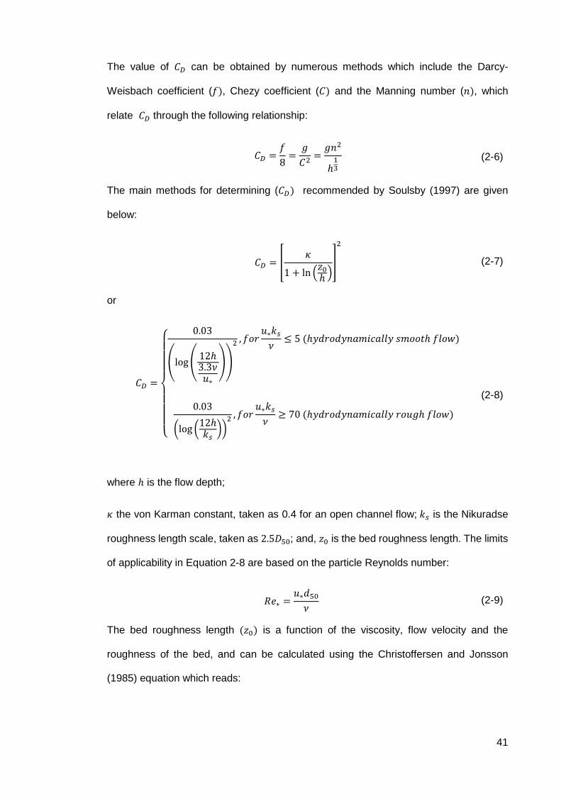
41

The value of 𝐶𝐷 can be obtained by numerous methods which include the Darcy-

Weisbach coefficient (𝑓), Chezy coefficient (𝐶) and the Manning number (𝑛), which

relate 𝐶𝐷 through the following relationship:

𝐶𝐷 =

𝑓

8=𝑔

𝐶2=𝑔𝑛2

ℎ13

(2-6)

The main methods for determining (𝐶𝐷) recommended by Soulsby (1997) are given

below:

𝐶𝐷 = [𝜅

1 + ln (𝑧0ℎ)]

2

(2-7)

or

𝐶𝐷 =

{

0.03

(log(12ℎ3.3𝜈𝑢∗

))

2

, 𝑓𝑜𝑟𝑢∗𝑘𝑠𝜈

≤ 5 (ℎ𝑦𝑑𝑟𝑜𝑑𝑦𝑛𝑎𝑚𝑖𝑐𝑎𝑙𝑙𝑦 𝑠𝑚𝑜𝑜𝑡ℎ 𝑓𝑙𝑜𝑤)

0.03

(log (12ℎ𝑘𝑠))2 , 𝑓𝑜𝑟

𝑢∗𝑘𝑠𝜈

≥ 70 (ℎ𝑦𝑑𝑟𝑜𝑑𝑦𝑛𝑎𝑚𝑖𝑐𝑎𝑙𝑙𝑦 𝑟𝑜𝑢𝑔ℎ 𝑓𝑙𝑜𝑤)

(2-8)

where ℎ is the flow depth;

𝜅 the von Karman constant, taken as 0.4 for an open channel flow; 𝑘𝑠 is the Nikuradse

roughness length scale, taken as 2.5𝐷50; and, 𝑧0 is the bed roughness length. The limits

of applicability in Equation 2-8 are based on the particle Reynolds number:

𝑅𝑒∗ =𝑢∗𝑑50𝜈

(2-9)

The bed roughness length (𝑧0) is a function of the viscosity, flow velocity and the

roughness of the bed, and can be calculated using the Christoffersen and Jonsson

(1985) equation which reads:

42

𝑧0 =𝑘𝑠30[1 − exp (−

𝑢∗𝑘𝑠27𝜈

)] +𝜈

9𝑢∗ (2-10)

2.2.2 Wave boundary layer

In the case of waves, the boundary layer has an oscillatory behaviour and reverses at

every half-cycle of the wave assuming that the water depth is sufficiently small (ℎ

𝐿< 0.5).

In this layer the amplitude of the orbital velocity increases from zero at the bed to the

value of the near bed orbital velocity (𝑈𝑤) at the top of the boundary layer. The value of

the bed orbital velocity can be determined using linear wave theory as:

𝑈𝑤 =

𝜋𝐻

𝑇tanh(𝑘ℎ) (2-11)

where 𝑘 is the wave number defined as 𝑘 =2𝜋

𝐿; 𝑇 is the wave period; 𝐻 is the wave

height; and, 𝐿 is the wavelength which can be determined iteratively using the following

expression:

𝐿 =

𝑔𝑇2

2𝜋tanh (

2𝜋ℎ

𝐿) (2-12)

For gravity waves the boundary layer does not exceed the thickness of a few

centimetres. Compared to steady flows this is O(100) smaller. In the absence of a steady

current the turbulence is contained within the boundary layer which in turn yields larger

bed shear stresses compared to a steady current. The bed shear stress for such a

boundary layer can be determined though the following expression:

𝜏𝑤 =

1

2𝜌𝑓𝑤𝑈𝑤

2 (2-13)

where 𝑓𝑤 is the wave friction factor which can be estimated by various methods, the most

widely used of which are presented below.

For hydrodynamically smooth boundary layers 𝑓𝑤 can be determined analytically via the

(Schlichting, 1968) method:

43

𝑓𝑤 =2√2𝜋𝜈𝛵

𝑈𝑤

(2-14)

For hydraulically rough flows, significantly more methods have been proposed. This is

because in most practical applications the boundary layer is rough.

Swart (1974) derived a semi-empirical expression for the determination of the wave

friction factor which reads as:

𝑓𝑤 = exp {−5.977 + 5.213 (

𝑈𝑤𝑇

2𝜋𝑘𝑠)−0.194

}

(2-15)

Myrhaug (1989) gives an implicit relationship for the friction factor which is based on

Christoffersen and Jonsson (1985) and can be solved iteratively:

0.32

𝑓𝑤= {ln(6.36

𝑈𝑤𝑇

2𝜋𝑘𝑠𝑓𝑤

12) − ln (1 − exp (−0.0262

𝑈𝑤𝑘𝑠𝜈

𝑓𝑤

12)} (2-16)

Nielsen (1992) suggests the following expression for the wave friction factor:

𝑓𝑤 = 𝑒𝑥𝑝 [(

5.5𝑈𝑤𝑇

2𝜋 𝑘𝑠)−0.2

− 6.3] (2-17)

Soulsby (1997) also recommends a formulation of the friction factor which was

developed through a best fit analysis from experimental data retrieved from seven

different sources. The expression reads:

𝑓𝑤 = 1.39 (

𝑈𝑤𝑇

2𝜋𝑧0)−0.52

(2-18)

Simons et al. (2001) conducted a number of experiments at different scales and

recommended the following expression:

𝑓𝑤 = 0.33 (

𝑈𝑤𝑇

2𝜋𝑘𝑠)−0.82

𝑓𝑜𝑟 𝑈𝑤𝑇

2𝜋𝑘𝑠< 30 (2-19)

44

Equation (2-19) also agrees with the findings of Dixen et al (2008) who found that the

friction factor is equal to:

𝑓𝑤 = 0.32 (

𝑈𝑤𝑇

2𝜋𝑘𝑠)−0.8

𝑓𝑜𝑟 0.2 <𝑈𝑤𝑇

2𝜋𝑘𝑠< 20 (2-20)

Dixen et al. (2008) also noted a phase difference between the free surface elevation and

the friction velocity. They recorded a phase difference ranging between 10° and 30°

which differs significantly from the laminar solution which yields 45° (Friedrichs and

Aubrey, 1994).

2.2.3 Wave current interaction

In most parts of the coastal and offshore environment waves and tidal currents co-exist.

The interaction between the two processes is not linear and thus a simple addition of any

aspect of their behaviour will not suffice. For the purpose of offshore structures two

interactions are of particular interest according to Soulsby (1997):

Wave current refraction which modifies the wavelength of the wave; and

Interaction of the boundary layer of waves and currents which leads to an

enhancement of the bed shear stress.

2.2.3.1 Wavelength modification

When waves propagate in the presence of a current their wavelength is modified, when

viewed from a stationary reference frame. This change is caused by the Doppler effect.

Thus by applying the Doppler principle to the dispersion relation for waves the following

expression is obtained:

(𝜔 − 𝑈𝑐 𝑘 cos(𝜑𝑑𝑖𝑟))

2 = 𝑔𝑘 tanh(𝑘ℎ) (2-21)

Where 𝜑𝑑𝑖𝑟 is the angle between the flow and the wave direction and 𝜔 is the absolute

radial frequency defined as:

𝜔 =

2𝜋

𝑇 (2-22)

45

The relative wave period of the combined wave and current (𝑇𝑟𝑒𝑙) can thus be estimated

by through the Doppler principle, which leads to:

𝑇𝑟𝑒𝑙 =

𝑐 + 𝑈𝑐𝑐

𝑇 (2-23)

where c is the wave celerity which is given:

𝑐 =

𝐿

𝑇 (2-24)

A change in the wavelength implies that the bed orbital velocity is also changed.

Therefore, the bed orbital velocity due to the change in the wavelength can be obtained

by substituting 𝑇𝑟𝑒𝑙 to Equation (2-11) which leads to the following expression:

𝑈𝑤 =

𝜋𝐻

𝑇𝑟𝑒𝑙𝑡𝑎𝑛ℎ(𝑘ℎ) (2-25)

2.2.3.2 Wave current boundary layer

The bed shear stress beneath waves and currents is enhanced in a non-linear way. This

means that the combined effects of waves and currents in the boundary layer cannot be

obtained by a simple superposition of the two. Soulsby (1997) mentions that there are

more than twenty models that describe this interaction. In a general case the total shear

stress of the flow can be divided into two components 𝜏𝑠 and 𝜏𝑓, where 𝜏𝑓 is the shear

stress contributed by the Reynolds stresses and 𝜏𝑠 is the component attributed to the

viscous shear stress. The latter usually contributes only a small amount of the bed shear

stress and thus can be neglected.

In a combined wave and current environment, the water column can be divided into three

zones according to Lundgren (1971). The first zone (I) located in the viscous sublayer

near the bed is dominated by the Reynolds stresses attributed to the wave orbital motion.

The thickness of this zone decreases for an increasing magnitude current. The second

zone (II) is characterised by the interaction of the viscous stresses attributed to both

waves and currents where the magnitudes of these forces are of the same order of

magnitude. Finally, the third zone (III) is ruled by the current-induced stresses. The above

46

characterisation of the water column suggests that the vertical distribution of the flow

velocities will also be affected and thus also the bed shear stresses (see Figure 2-2).

Figure 2-2: Definition sketch and zones of turbulence (proposed by Lundgren, 1971).

As mentioned above, there are different methods for determining the combined effects

of waves and currents on the bed shear stress (e.g. Fredsøe and Deigaard, 1992;

Soulsby et al., 1993; and Soulsby and Clarke, 2005). In this section only the method

proposed by Soulsby et al. (1993) is presented, as it provides an algebraic approximation

to most of the models which is accurate to 5% in most cases (Soulsby, 1997).

𝜏𝑚𝑒𝑎𝑛 = 𝜏0 (1 + 1.2 (

𝜏𝑤𝜏0 + 𝜏𝑤

)3.2

) (2-26)

𝜏𝑚𝑎𝑥 = ((𝜏𝑚𝑒𝑎𝑛 + 𝜏𝑤 cos𝜑𝑑𝑖𝑟)

2 + (𝜏𝑤 sin𝜑𝑑𝑖𝑟)2)0.5 (2-27)

Where 𝜑𝑑𝑖𝑟 is the angle between the flow and wave direction.

According to Soulsby (1997) the maximum bed shear stress (𝜏𝑚𝑎𝑥) should be used for

calculations involved in the determination of incipient sediment motion, while the mean

47

bed shear stress (𝜏𝑚𝑒𝑎𝑛) should be used when determining sediment diffusion, both of

which are relevant to scour processes.

2.2.4 Incipient motion of sediment particles

It is of importance first to identify and understand the forces that act on a sediment

particle in order to study the process of incipient motion. When a stationary sediment

particle is in contact with any flow the sum of the forces acting on it need to be in balance;

if not in balance the particle will be in motion. Three main forces can be identified: contact

forces from other particles 𝐹𝑠, weight (𝑊) and the hydraulic forces which include drag

(𝐹𝐷) and lift (𝐹𝐿).

𝐹𝑠 and 𝑊 are related to the weight of the particle acting at its centre of gravity in the

vertical direction. It can be determined by multiplying the volume of the particle with the

specific weight of the particle. The contact forces are basic reactions exerted by the

particles against which the element rests. The magnitudes of these forces are a function

of the weight and shape of the particle as well as the resulting fluid force.

Figure 2-3: Definition sketch of forces acting on a single sediment particle.

The fluid forces acting on the particle are more complicated and will be treated separately

below.

For steady currents, the drag force acting on a particle is given by the following

expression:

48

𝐹𝐷 =

1

2𝜌𝐶𝐷𝐴𝑝𝑈𝑐|𝑈𝑐| (2-28)

where 𝐶𝐷 is the drag coefficient, which is a function of the particle Reynolds number and

varies between 0.5 for wave dominated flow conditions and 1.5 for current dominated

conditions (Dixen et al., 2008).

𝐴𝑝 is the area of the particle which is exposed to the flow.

In the case of oscillatory flow, there are two additional contributions to the total fluid force:

𝐹𝐷 =

1

2𝜌𝐶𝐷𝐴𝑝𝑢|𝑢| + 𝐶𝑚𝜌𝑉𝑝

𝑑𝑢

𝑑𝑡+ 𝜌𝑉𝑝

𝑑𝑢

𝑑𝑡

(2-29)

where 𝑉𝑝 is the volume of the particle; 𝑢 could be the orbital velocity, the combined wave-

current velocity near the bed or the steady current; 𝐶𝑚 is the inertia coefficient which

takes the value of 0.5 for the range of the sediment Reynolds number involved in most

sediment transport and scour protection problems (Massey and Smith, 1998).

The second term on the right hand side of Equation (2-29) is the hydrodynamic mass

force which is caused by the acceleration of the fluid in the surrounding of the body. The

third term is known as the Froude-Krylov force, which is produced by the pressure

gradient acting on the particle.

The lift force acting on a sediment grain is attributed to four factors according to Vithana

(2012):

Vortex shedding at the lee of the particle;

The influence of the pressure gradient induced by other stones ahead of the

particle;

Eddies and turbulence induced by other surrounding grains; and

Quasi steady upward drag induced by the flow alteration created by other

particles.

The uplift forces can be determined using a similar Equation to (2-28):

49

𝐹𝐿 =

1

2𝜌𝐶𝐿𝐴𝑝𝑢|𝑢| (2-30)

where 𝐶𝐿 is the lift coefficient taking a value between 0.1-0.2 for a sphere placed between

other particles in both unidirectional and oscillatory flows (Torum et al., 1992).

The approach described above for determining the initiation of sediment movement

based on the balance of forces in practical terms is very difficult to achieve, due to the

irregularity of the shape of sediment particles. In addition, the continuous movement of

sediment and the effects other particles have on the flow cause further uncertainties in

the calculation of the forces (Hofland, 2005). This causes the point of application of the

forces to change continuously and thus cannot provide a consistent way of determining

incipient motion.

Shields (1936) developed a method for determining the incipient motion of sediment

based on the bed shear stress exerted by the flow on a flat bed comprised of a

homogeneous sediment. In order to make his method dimensionally homogeneous he

proposed the non-dimensional form of the critical bed shear stress required to initiate

incipient motion (𝜃𝑐𝑟) as:

𝜃𝑐𝑟 =

𝜏𝑐𝑟𝑔 (𝜌𝑠 − 𝜌)𝑑50

(2-31)

where 𝜏𝑐𝑟 is the bed shear stress required to initiate sediment motion.

In his original work he proposed that 𝜃𝑐𝑟 is a function of the grain Reynolds number (𝑅𝑒∗)

(Figure 2-4) which is defined as:

As can be seen in Figure 2-4 𝑢∗ is present in both the vertical and horizontal axes.

Keeping in mind that 𝑢∗ and 𝜏0 are linked to each other with equation (2-1), this makes

the estimation of the critical shear stress difficult due to the implicit nature of the Shields

graph.

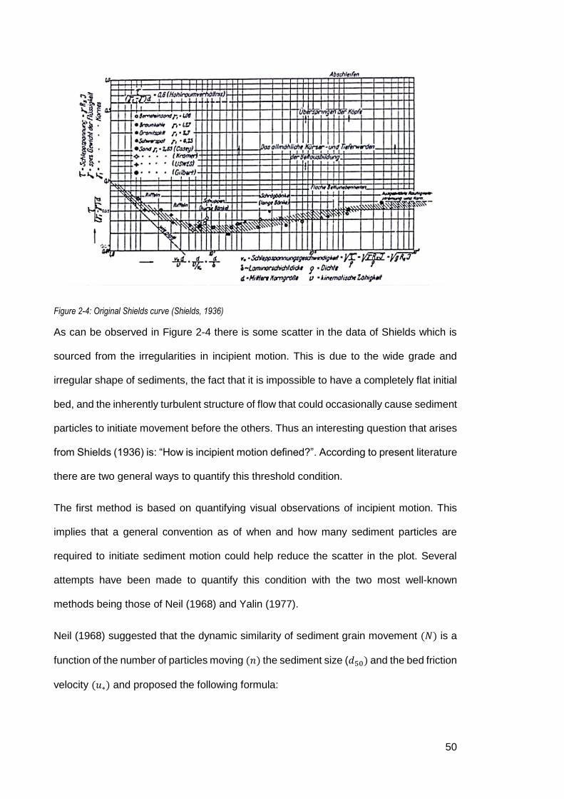
50

Figure 2-4: Original Shields curve (Shields, 1936)

As can be observed in Figure 2-4 there is some scatter in the data of Shields which is

sourced from the irregularities in incipient motion. This is due to the wide grade and

irregular shape of sediments, the fact that it is impossible to have a completely flat initial

bed, and the inherently turbulent structure of flow that could occasionally cause sediment

particles to initiate movement before the others. Thus an interesting question that arises

from Shields (1936) is: “How is incipient motion defined?”. According to present literature

there are two general ways to quantify this threshold condition.

The first method is based on quantifying visual observations of incipient motion. This

implies that a general convention as of when and how many sediment particles are

required to initiate sediment motion could help reduce the scatter in the plot. Several

attempts have been made to quantify this condition with the two most well-known

methods being those of Neil (1968) and Yalin (1977).

Neil (1968) suggested that the dynamic similarity of sediment grain movement (𝑁) is a

function of the number of particles moving (𝑛) the sediment size (𝑑50) and the bed friction

velocity (𝑢∗) and proposed the following formula:

51

𝑁 =

𝑚𝑑503

𝑢∗ (2-32)

Yalin (1977) adopted an analytical approach for quantifying the incipient motion which is

based on an assumption that the probability of detachment of a particle from the bed

follows a normal distribution. The expression he derived reads as:

휀 =𝑚

𝐴𝛺𝑡√𝜌𝑑50𝛾𝑠 − 𝛾

(2-33)

where 𝐴𝛺 is the area considered in the observation; 𝑡 is the time period in which

observations are made; and 𝛾𝑠 and 𝛾 are the specific weight of the sediment and water

respectively.

Yalin (1977) suggests that a practical value of 휀 = 10−6 in order to be able to compare

results from different studies effectively.

The second way of quantifying the threshold condition for sediment motion is by

determining the sediment transport rate at which incipient motion occurs. This method

involves the arbitrarily definition of a small non-dimensional unit transport rate that

corresponds more closely to the transport rate observed in most of the existing

publications. An example of such work is Whitehouse and Hardisty (1988) who

investigated the effect of bed inclination on the threshold of sand transport over

submarine slopes.

The Shields diagram was updated with additional data from experiments by Miller et al.

(1977) in order to increase its range of validity for a wider range of particle Reynolds

numbers (Figure 2-5). The direct conclusion of their work was that the Shields curve

shifted to smaller values of 𝜃𝑐𝑟 for 𝑅𝑒∗ values greater than 10.

52

Figure 2-5: Modified Shields diagram (Miller et al., 1977)

Soulsby and Whitehouse (1997) modified the original Shields diagram to make it explicit.

In the new method the Shields parameter is plotted against the non-dimensional grain

size defined as:

𝐷∗ = [𝑔 (𝜌𝑠𝜌 − 1)

𝜈2]

13

𝑑50 (2-34)

In the same graph additional data from waves, currents and combined waves and

currents were plotted, thus extending its range. (Soulsby and Whitehouse, 1997)

developed an algebraic expression for the original Shields curve. They further developed

a second algebraic expression to account for smaller sediment sizes and found that the

original Shields paper overestimated by as much as O(10) the Shields parameter for very

small values of 𝐷∗ (Figure 2-6).

Figure 2-6: Updated Shields diagram (Source: Soulsby, 1997)

53

The dotted line in Figure 2-6 is given by the following expression:

𝜃𝑐𝑟 =

0.30

1 + 1.2𝐷∗+ 0.055[1 − exp(−0.020𝐷∗)] (2-35)

Many more studies have been reported where the Shields diagram has been modified

or improved by the addition of new data-points. The reader is directed to the publications

of (Vanoni, 1964; Buffington and Montgomery, 1997; Hoffmans and Verheij, 1997) who

also contributed towards clarifying several aspects of the original Shields diagram.

It is also important to mention the work of (Hjulstrom, 1939) who developed a graph

where the different velocities correspond to erosion, transportation and deposition of

fluvial sediments (Figure 2-7). The main difference between Hjulstrom and the Shields

diagram is that Hjulstrom plots the mean flow velocity against the sediment diameter

rather that the non-dimensional bed shear stress and 𝑅𝑒∗. This is the reason why multiple

lines corresponding to different water depths (0.01 to 10m) are plotted on the graph. This

graph is explicit and thus is easy to interpret. But the fact it is dimensional makes it prone

to temperature and density changes and thus has not been commonly used by

designers.

Figure 2-7: Sundborg’s modification of the Hjulström diagram. (After Sundborg, 1956.)

54

2.2.5 Threshold current speed

The threshold of motion speed of sediments (𝑈𝑐𝑟) is an important parameter for any

sediment transport process. 𝑈𝑐𝑟 is the mean flow required to move a sediment particle

over a flat bed. It is particularly important for scour and scour protection design and this

section will provide an overview of some of the main methods that can be used to

determine it.

For a steady current Van Rijn (1984) proposed:

𝑈𝑐𝑟 = 0.19𝑑500.1 log (

4ℎ

𝑑90) 𝑤𝑖𝑡ℎ 100 ≤ 𝑑50 ≤ 500𝜇𝑚 (2-36)

𝑈𝑐𝑟 = 8.5𝑑500.6 log (

4ℎ

𝑑90) 𝑤𝑖𝑡ℎ 500 < 𝑑50 ≤ 2000𝜇𝑚 (2-37)

This method is an effective way for determining the threshold velocity but is only valid for

non-cohesive sediment up to the size of coarse sand. This provides a limitation with

regards to its application to larger grains such as the ones used for scour protection.

A second method proposed by Soulsby (1997) is based on combining the critical Shields

parameter and the friction law. This yields a method that is valid throughout the entire

range covered by the Shields diagram and reads as:

𝑈𝑐𝑟 = 7(ℎ

𝑑50)

1

7[𝑔(𝑠 − 1)𝑑50𝜃𝑐𝑟] (2-38)

2.3 Hydrodynamics around cylindrical structures

The local sediment transport around offshore structures is influenced by the flow

structure interaction and the resulting changes in the local flow field. Extensive research

on the hydrodynamic phenomena around monopiles has been conducted in the past, but

much less is known about the hydrodynamic response to more complex structures such

as GBFs.

According to (Sumer and Fredsøe, 2002) four phenomena are observed when a flow

interacts with a monopile (Figure 2-8):

55

The downflow along the face of the structure;

The horseshoe vortex system that originates at the front of the structure and

circles around it;

The lee-wake vortex shedding which is caused by flow separation along the

periphery of the structure; and

The local contraction of the flow around the structure.

Figure 2-8: Flow structure interaction definition sketch (source: Roulund et al., 2005)

These processes cause a local increase in the bed shear stress. This increase relative

to the undisturbed case is described by the bed shear stress amplification factor defined

as:

𝑎 =𝜏𝑏𝜏∞

(2-39)

Here 𝜏∞ is the undisturbed bed shear stress which can be determined from Equation (2-

5) for currents, and Equation (2-12) for waves; 𝜏𝑏 is the local bed shear stress at a

location near the structure.

56

2.3.1 Downflow

The downflow in front of the pile is caused by a stagnation point on the centreline of the

face of the structure, which is measured from the original bed (y in Figure 2-9). The

stagnation point forces a portion of the flow to move upwards which causes the surface

bow wave. The remaining portion of the flow is then directed towards the bed causing a

downwards jet (downflow) which feeds into the horseshoe vortex (see Figure 2-9). The

energy at the face of the structure is the sum of the kinetic and the static energy

components. This means that in shallow waters the hydrostatic component of the total

energy is small compared to the kinetic which translates into a stagnation point further

away from the bed. Scour under such conditions is called shallow water scour and is

highly dependent on the water depth. When the water depth is relatively large compared

to the structure’s diameter the stagnation point shifts closer to the bed which yields a

more evenly distributed downflow and upflow jet. Scour under this condition is named

deep water scour and is independent of the water depth.

Figure 2-9: Definition sketch of downflow phenomenon (location of the stagnation point is arbitrarily selected in this image)

57

2.3.2 Horseshoe vortex

The horseshoe vortex plays a significant role in scour development and sediment

transport. It is created by the rotation of the incoming flow and is caused by the three-

dimensional separation of the incoming flow due to the adverse pressure gradient

induced by the structure (Sumer and Fredsøe, 2002). The separated boundary layer then

forms a spiral vortex which wraps around the structure and is carried away by the main

current forming a horseshoe shape in the plan view (see figure 2-8).

2.3.2.1 Horseshoe vortex in currents

In the case of a unidirectional and steady current the horseshoe vortex has been

investigated by numerous authors (see Baker 1978; 1979; 1980; 1985; 1991; Dargahi,

1989; Graf and Yulistiyanto, 1998; and Roulund et al., 2005). The studies of Baker and

of Hjiorth (1975) showed that under the forcing of a unidirectional current the

amplification of the bed shear stress can be increased up to a factor of 11. The magnitude

of this amplification may be challenged, though, due to the methods used to measure

the local bed shear stress. Nevertheless, these studies showed that the local bed shear

stress experiences significant amplification which drives the sediment transport and is

thus an important contributing factor for the scour process.

According to Baker (1978, 1979 and 1980) the horseshoe vortex is characterised by

three key non-dimensional quantities:

The pile Reynolds number (𝑅𝑒𝐷);

The relative thickness of the boundary layer (𝛿/𝐷); and

The local adverse pressure gradient.

The pile Reynolds number is defined as:

𝑅𝑒𝐷 =

𝑈𝑐𝐷

𝜈

(2-40)

where 𝐷 is the pile diameter.

The pile Reynolds number describes the viscous forces of the flow relative to the inertial

forces. This means that if in a specific scenario high viscous forces are anticipated (i.e.

58

small 𝑅𝑒𝐷) then the boundary layer separation will be delayed, resulting in smaller

horseshoe vortex system. Roulund et al. (2005) conducted a series of numerical and

experimental investigations and concluded that the size and intensity of the horseshoe

vortex increases up to a 𝑅𝑒𝐷 value of 500 and then decreases for an increasing value of

the pile Reynolds number (Figure 2-10). This decrease in the size of the horseshoe

vortex for larger values of 𝑅𝑒𝐷 is attributed to the increased momentum exchange

between the layers of the fluid in the turbulent boundary layer.

Figure 2-10: Influence of the 𝑅𝑒𝐷 on the Horseshoe vortex (source: Roulund et al., 2005)

59

Similar to the pile Reynolds number the thickness of the undisturbed boundary layer also

effects the formation of the boundary layer. It can be understood that the separation of

the boundary layer will be delayed (i.e. smaller horseshoe vortex) if the approaching

boundary layer is more uniform. This has been verified by Roulund et al. (2005) among

other publications (Figure 2-11), they predicted accurately the separation distance of the

horseshoe vortex but not as well the amplification of the bed shear stress, which is most

probably linked to the choice of turbulence model in the study. The study concluded that

the horseshoe vortex increases in size and intensity up to certain point and then reaches

a plateau which is dependent on the pile Reynolds number.

Figure 2-11: Influence of the boundary layer thickness on the Horseshoe vortex for 𝑅𝑒𝐷 = 2 ∗ 102, line: result of

numerical model, x symbol: experimental measurement (source: Roulund et al., 2005).

The final factor influencing the horseshoe vortex in the case of a unidirectional current is

the adverse pressure gradient. When the flow profile does not change, the pressure

τsD

τmaxτ∞

60

gradient is a direct function of the shape of the structure. This means that a more

streamlined structure geometry will result in a smaller horseshoe vortex compared to a

uniform cylinder. Sumer et al. (1997) reported values of the separation point along the

centreline of different cross-sectional shapes (taken in the planar view point) the results

of which are shown in Figure 2-12. The study showed that the orientation of a rectangular

foundation can results in a reduction in the size of the horseshoe vortex by a factor of

15%.

Figure 2-12: Boundary layer separation distance for different cross-sectional shapes (source: Sumer et al., 1997)

In addition, the lateral shape and dimension of the structure significantly influences the

horseshoe vortex size. Chou and Chao (2000) investigated the characteristics of the

horseshoe vortex around non surface piercing rectangular foundations. Their study

showed that the horseshoe vortex system breaks up into a series of smaller regularly

shaped vortices when the aspect ratio of the foundation (𝑊/ℎ𝑐 ) exceeded the value of

10. More regular vortices yield a smaller amplification of the bed shear stress and thus

smaller sediment transport capacity. Here 𝑊 is the cross flow width of the foundation

and ℎ𝑐 is the height of the foundation. Further studies on the effects of conical based

foundation on the amplification of the bed shear stress conducted by Sumer et al. (1994)

61

revealed that the amplification of the bed shear stress increases as the side slope of the

conical based structures increases. This finding was also supported by the findings of

Tavouktsoglou et al. (2015) who reported the amplification of the bed shear stress

around cones.

2.3.2.2 Horseshoe vortex in waves

According to Sumer and Fredsøe (2002) the presence of waves introduces one

additional non-dimensional quantity, the Keulegan-Carpenter number (𝐾𝐶). The

Keulegan-Carpenter number is a non-dimensional quantity which describes the relative

importance of the drag over the inertial forces and is defined as:

𝐾𝐶 =

𝑈𝑤𝑇

𝐷=2𝜋𝑎𝑤𝐷

(2-41)

Here 𝑈𝑤 is the amplitude of the bed orbital velocity, 𝑇 the wave period, 𝐷 the diameter

of the cylinder and 𝑎 is the amplitude of the wave.

The expression in equation (2-41) implies that when the 𝐾𝐶 is small (i.e. smaller than 6)

the stroke of the wave is small relative to the diameter of the pile and thus a horseshoe

vortex is not expected to develop. On the other hand if 𝐾𝐶 is large (greater than 60) then

the orbital motion is much greater than the diameter of the structure which means that

the horseshoe vortex in this case should resemble the vortex system induced by a

unidirectional current (Sumer and Fredsøe, 2002).

The horseshoe vortex in waves is not present at all phases of the wave cycle. It emerges

sometime after the flow reverses and it ceases of existence before the flow reverses

again (Sumer et al., 1997). The life span of the horseshoe vortex is also dependent on

the 𝐾𝐶 number according to same study (Figure 2-13). Figure 2-13 also shows that the

crest of the wave has the tendency to induce larger horseshoe vortices compared to the

trough. This difference is attributed to the asymmetry in the wave itself which tends to

follow Stokes’ wave theory in most flume tests.

62

Figure 2-13: Horseshoe vortex in different phases of wave cycle (Source: Sumer et al., 1997)

The horseshoe vortex in waves for non-uniform cross section structures is a subject

which has not been investigated in the literature. This is a clear gap in the knowledge

which needs to be filled in order to understand in more depth the scour process around

such structures in waves.

2.3.2.3 Horseshoe vortex in combined waves and currents

According to Sumer et al. (1997) the lifespan of the horseshoe vortex increases as the

ratio of the current velocity to the bed orbital velocity (𝑈𝑐/𝑈𝑤 ) increases. Figure 2-14

shows that the horseshoe vortex is created for smaller values of the 𝐾𝐶 number, and

below the critical value of 6 in waves alone, as the current flow speed increases when

the current is following the wave.

63

Figure 2-14: Presence of horseshoe vortex in phase space: influence of superimposed current (Source: Sumer et al., 1997)

Further to the study of Sumer et al. (1997); Umeda et al. (2003) conducted a series of

computational simulations where the horseshoe vortex was measured around cylinders

for combined waves and currents, with waves that were following and opposing the

current. Their study showed that in the case where the waves followed the main current

a strong horseshoe vortex developed at the leading edge of the structure. In the case

were the waves where opposing the current a smaller horseshoe vortex developed at

the leading edge of the structure and no vortex system developed on the lee side. Their

results showed that the horseshoe vortex system increases in size for an increasing

value of 𝐾𝐶 or 𝑉𝑡 = 𝑈𝑐/𝑈𝑤 , which agrees with the general findings of Sumer et al.

(1997). Further to this they proposed an empirical equation that relates the flow

separation distance (𝑥𝑠) in front of the structure to the non-dimensional quantity 𝐴0,

which is shown in figure 2-15. 𝐴0 is defined as:

64

𝐴0 = 𝐾𝐶2 + 𝜋

𝑈𝑐𝑈𝑤

4𝜋

(2-42)

Figure 2-15:Separation distance for combined waves and currents (Source: Umeda et al., 2003)

2.3.3 Lee-wake vortex

2.3.3.1 Lee-wake vortex in currents

Sumer and Fredsøe (1997) provide a comprehensive review of the lee-wake

phenomenon around cylindrical structures which important for scour in currents. The lee-

wake vortex is a function of the pile Reynolds number with the main regimes summarised

in Figure 2-16. The most important phenomenon in the lee-wake region is named vortex

shedding, which occurs for 𝑅𝑒𝐷 > 40. In this range of Reynolds number, the boundary

layer on the outer face of the cylinder separates due to the adverse pressure gradient.

The vorticity in the boundary layer is then fed into the shear layer at the lee of the

structure creating a streak of asymmetric vortices that are carried downstream with the

main current. The vortex shedding phenomenon continues to occur for as long as the

two shear layers occurring on each side of the cylinder interact.

65

Figure 2-16: Lee wake vortex shedding regimes around a cylinder (source: Sumer and Fredsøe, 1997)

The non-dimensional form of the vortex shedding frequency is known as the Strouhal

number (𝑆𝑡) defined as:

𝑆𝑡 =𝑓𝑣𝐷

𝑈𝑐 (2-43)

𝑆𝑡 and thus the turbulence level at the lee of the structure has been found to be a function

of the pile Reynolds number and is shown in the following figure (Figure 2-17).

66

Figure 2-17: Strouhal number as a function of the pile Reynolds number for smooth and rough cylinders (Data source: Roshko, 1961)

As well as the roughness of the body the cross-flow shape of the structure also effects

the Strouhal number due to the change of the pressure gradient induced by the structure.

The relationship of the Reynolds number with different 2D uniform geometries is given

by Blevins and Burton (1976) and is shown in figure 2-18. For non-cylindrical geometries

with 𝑅𝑒𝐷 > 104 the Strouhal number is not expected to undergo any further variations as

the separation point is fixed.

Figure 2-18: Effect of cross-flow shape on the Strouhal number (Source: Blevins and Burton, 1976)

In addition to the factors mentioned in the preceding paragraphs Sumer and Fredsøe

(1997) suggest that an increasing level of incoming turbulence would result in an overall

increase in the Strouhal number for the entire range of Reynolds numbers. The same

effect also occurs when the shear gradient in the approach flow increases according to

Kiya et al. (1980).

67

2.3.3.2 Lee-wake vortex in waves

In the case of waves the lee-wake process has a secondary role with regards to scour,

with the horseshoe vortex governing the scour process (Sumer and Fredsøe, 2002). For

waves, 𝐾𝐶 becomes an influencing parameter in the lee-wake process. The six main

flow separation regimes around a cylinder are summarised in Figure 2-19. The 𝐾𝐶

ranges in the following figure were derived for a pile Reynolds number of 103. Sumer

and Fredsøe (1997) provide two additional graphs based on a compilation of

experimental studies to describe the dependence of these regimes on both the 𝐾𝐶 and

𝑅𝑒𝐷 (Figures 2-20 and 2-21).

As can be understood from the figures, in the case of waves it is difficult to define the

vortex shedding frequency (𝑓𝑣). One way of defining the vortex shedding frequency is by

calculating the lift frequency power spectrum and then determining the dominant lift

frequency (𝑓𝐿). The non-dimensional form of the lift frequency is then defined by

Equation (2-44):

𝑁𝐿 =𝑓𝐿

𝑓𝑤𝑎𝑣𝑒 (2-44)

Here 𝑓𝑤𝑎𝑣𝑒 is the wave frequency.

Figure 2-19: Regimes of flow separation around cylinders in waves (source: Sumer and Fredsøe, 1997)

68

Figure 2-20: Flow separation regimes for small 𝐾𝐶 and very small 𝑅𝑒𝐷 numbers (source: Sumer and Fredsøe, 1997)

Figure 2-21: Flow separation regimes for large 𝐾𝐶 and 𝑅𝑒𝐷 numbers (source: Sumer and Fredsøe, 1997)

One more important consequence of the lee-wake phenomenon that particularly

concerns large diameter structures is steady streaming. In this case four recirculating

Figure 2-20

69

flow cells (one in each quadrant) are created (Figure 2-22) due to the unseparated

oscillatory flow.

Figure 2-22: Definition sketch of steady streaming

Wang (1968) developed a semi-analytic theory that predicts the size of the recirculating

cell (Δ in Figure 2-22) for small values of Reynolds number. The solution shows that the

largest recirculating cells occur for a combination of large 𝐾𝐶 and small 𝑅𝑒 which is in

accordance with potential flow theory.

Figure 2-23: Size of steady streaming cell (Reproduced from Wang, 1968)

𝑟0

70

2.3.4 Streamline contraction

According to classical hydrodynamics streamline contraction is caused by the presence

of the structure which reduces the cross-sectional area through which the flow passes,

and this causes a local acceleration of the flow, which in turn causes the amplification of

the bed shear stress to increase significantly. According to Hjorth (1975) the combined

effect of the horseshoe vortex with streamline contraction can result in amplifications of

the bed shear stress up to a factor of 10.

2.4 Scour around cylindrical structures

Changes in the flow pattern around lead to an increase in the local velocities and

turbulence, which increase the sediment transport capacity of the flow. An equilibrium

condition may then be achieved as the local hydraulic conditions are adjusted through

the scour process. Here scour is defined as the erosion of sediment around a structure.

This section provides an overview of the key literature and physics that are associated

with the scour around both uniform and non-uniform cylindrical structures.

2.4.1 Scour types

Scour around structures can be divided into two main types of scour, general (or global)

scour and local scour. These two scour processes have different time and length scales.

The total scour can then be determined as the sum of the two components (local and

global). Figure 2-24 present a diagram of the basic variables involved in the scour

process for monopiles in unidirectional currents. Here h is the flow depth; D the diameter

of the pile; U(z) the velocity profile S the scour depth takes as the local change in depth

near the structure from the original bed level; 𝜑𝑢𝑝 and 𝜑𝑑𝑜𝑤𝑛the upstream and

downstream slope of the scour hole; and 𝑊𝑠𝑐𝑜𝑢𝑟 the total width of the scour hole.

71

Figure 2-24: Definition sketch of local scour around monopile in unidirectional flow.

2.4.1.1 General (global) scour

The time-scale of global scour tends to be longer compared to the corresponding for

local scour. General scour can be attributed to two physical phenomena (Hoffmans and

Verheij, 1997):

Overall degradation of the bed; and,

Contraction scour.

Overall Degradation

Overall degradation results from the inherent flow conditions at a given location or from

the modification of the stable flow regime. Examples of features that result in such

degradation are:

Storm surges in coastal waters;

Dredging and land reclamation in coastal waters;

Sand waves; and,

Flood events in rivers and estuaries.

72

The result of the overall degradation at foundations will be the lowering of the bed which

introduce additional failure risks that may lead to the complete failure of the foundation.

It should be noted that human interventions may also lead to aggradation which may

result in the reduction of scour risk.

Contraction scour

Contraction scour occurs due to the reduction of the cross-sectional area where the flow

naturally passes, which causes a local increase in the flow velocities. This results in the

general lowering of the bed across the entire width of the control volume. Examples of

contraction scour are:

The scour by blockage induced by a composite structure such as a jacket

foundation;

Closure works and multiple bridge footings; and,

River bridge embankments.

2.4.1.2 Local scour

Local scour is the result of the impact the structure or a structural element (when

considering composite structures) has on the local hydrodynamics. Given that global

scour is very site specific (Hansen and Gislason, 2005) local scour is the most

researched scour type. Physical and prototype model testing can be used for the

development of scour prediction equations for different types of structure. When

considering more unusual structures, physical modelling results can be used for

obtaining the appropriate information required for the design. When considering local

scour problems, the equilibrium scour depth is the most relevant parameter, especially

when isolated structures (bridge piers, offshore foundations etc.) are considered

(Hoffmans and Verheij, 1997). The time development of scour is of importance in some

cases, examples of which are post-installation monitoring, closure works, and temporary

installations such as cofferdams among other hydraulic engineering applications.

73

2.4.2 Sediment transport in local scour

Local scour around structures can be distinguished into two categories based on the

upstream sediment transport:

Clear water scour (black line in Figure 2-25), occurs when the bed material

upstream of the structure is not in motion. The sediment transported into the

contracted section is essentially zero. Generally, under clear-water scour, no

refilling of the scour hole occurs lack of sediment supply. With regards to scour

evolution the equilibrium scour depth is reached asymptotically with time; and,

Live bed scour (black line in Figure 2-25), which is where sediment transport

exists throughout the domain. Sediment particles are transported from

upstream of the structure into the scour hole. This forces the equilibrium scour

hole to be smaller compared to the clear water mode. In this case the scour

depth increases rapidly with time and then fluctuates about an average

equilibrium scour depth.

Figure 2-25: Scour depth evolution, live bed Vs clear water scour.

In clear water scour four scour evolution phases have been identified according to

Breusers (1965) (see Figure 2-26).

In the initial phase the flow in the scour hole is nearly uniform in the streamwise direction.

During this phase the scour process is the most rapid with sediment being eroded

74

quickly, and in some cases suspended into the water column. Some of the suspended

sediment particles are transported with the main flow and the lee wake vortex shedding

and deposited at the lee of the structure. In addition, sediment is eroded in the form of

bed load. In this phase the scour hole width and length increase considerably.

The second phase of the scour process is the development phase. During this phase the

scour hole geometric shape does not change considerably. The depth and width of the

scour hole continue to grow at a constant rate according to observations reported by

Hoffmans (1990), while the lower part of the scour hole (near the structure) continues to

change due the turbulent bursts induced by the horseshoe vortex. Furthermore, the

suspended sediment load decreases considerably and the main part of the erosion is

carried through bed-load transport.

The third phase is the stabilization. In this phase the rate of scour decreases in time. The

erosion potential within the scour hole is small, with the width of the scour hole increasing

more relative to the scour depth. Finally, equilibrium (phase 4) is achieved when the

dimensions of the scour hole do not change significantly with time.

Figure 2-26: Development of clear-water scour (Derived from: Hoffmans and Verheij, 1997)

75

2.4.3 Scour in steady unidirectional currents

Many studies have been conducted to investigate the scour around cylindrical structures,

particularly in the context of scour around bridge piers. Some key studies include Hjorth

(1975), Melville (1975), Breusers et al. (1977), Ettema (1980), Melville and Sutherland

(1988) and Melville and Raudkivi (1996). Extensive reviews on the topic can also be

found in Hoffmans and Verheij (1997), Whitehouse (1998), Melville and Coleman (2000)

and Sumer and Fredsøe (2002).

Table 2-1 presents additional publications that were used in this study for the derivation

of a new scour prediction equation.

Table 2-1: Representative studies on scour around uniform cylinders used in this study.

Study Key findings.

Shen et al (1969) Investigated the influence of the pile Reynolds number.

Jain and Fischer (1979) Investigated scour at high Froude numbers which typical of river

environments.

Ettema (1980)

Found that variations in scour depth around monopiles is a function are

related to the comparative pier and particle diameters, approach flow

depths, and the particle size distribution of a sediment.

Yanmaz and Altinbilek

(1991)

The study found that the shape of the scour hole around bridge piers

remains almost unchanged with respect to time.

Dey et al (1995) Studied the dependence of the scour hole shape with the horseshoe

vortex.

Melville, B. W. (1997) Presented a large number of experimental results on scour around bridge

piers and developed correction factors for the prediction of the equilibrium

scour depth around them.

Melville and Chiew (1999) Investigated the effect of the flow duration on the shape and depth of the

scour hole.

Sheppard et al (2004) Investigated large scale scour around monopiles and found that the

equilibrium scour depths were found to depend on the wash load

concentration.

Ettema et al (2006) Presented the effect of large scale turbulence on scour behaviour.

Sheppard and Miller (2006) Conducted a number of large scale experiments and compared the

accuracy of predictive equations.

Mututano et al (2013) Compiled a database of equilibrium scour depths in the North sea and

evaluated the predictive ability of existing design equations.

76

2.4.3.1 Influencing parameters

In steady currents, the governing hydrodynamic process has been identified to be the

horseshoe vortex (Whitehouse, 1998). Thus the scour process around uniform cylinders

has mainly been researched with respect of the behaviour of the horseshoe vortex and

the effect the different flow conditions have on it. According to Dargahi (1989) the size of

the horseshoe vortex is independent of the flow condition and depends only on the

diameter of the structure. More specifically, Muzzammil and Gangadhariah (2003)

showed the diameter of the primary vortex is equal to about 20% of the pile diameter.

After the formation of the horseshoe vortex sediment starts to be transported once the

locally induced pressure gradient is high enough to mobilise the sediment, which creates

a scour hole. The size of the horseshoe vortex increases linearly for an increasing scour

hole depth (Dey and Raikar, 2007; Muzzammil and Gangadhariah, 2003), while the

intensity of the horseshoe vortex decreases (Dey and Raikar, 2007). A weaker

horseshoe vortex means that the sediment transport capacity of the local flow decreases

while it also has a steep slope to travel in order to exit the scour hole. Therefore, this can

explain the decreasing scour rate in the scour development curve (see Figure 2-25).

More recently a secondary mechanism that effects the scour phenomenon in

unidirectional steady currents has been identified, namely, the counter-rotating

streamwise phase-averaged vortices (LSCSVs) (see Figure 2-27). The LSCSVs are

mainly driven by the longitudinal counter-rotating vortices which are created partly by the

horseshoe vortex and the variation of the shedding frequency over the height of the

structure (Baykal et al., 2015). These vortices effectively pickup sediment (in the form of

suspended load) from the lee of the structure and transport it further away, thus

increasing the scour potential. It should be noted that the effectiveness of the LSCSV in

transporting material away from the structure should also be affected by the ability of the

flow to keep it suspended while it is advected by the mean flow and this vortex system.

Thus, for a certain set of flow conditions, sediments with a larger settling velocity (𝑤𝑠)

77

would be deposited closer to the structure, while sediments with a lower 𝑤𝑠 would be

advected further away.

Figure 2-27: Counter-rotating streamwise phase-averaged vortices (a) streamlines (b) mean vorticity in x- direction (Source: Baykal et al., 2015)

The previous paragraphs show that the scour around a cylinder is dependent on the

horseshoe vortex and on the lee wake vortex shedding. Therefore, the scour process

should be influenced by the physical quantities that describe these processes and the

quantities that describe the sediment’s ability to resist these processes. Based on

existing knowledge the following quantities have been identified as the most influencing

and have been extensively researched:

The sediment mobility ratio;

Relative flow depth; and,

Sediment gradation.

The following paragraphs explain the influence these parameters have on the scour

process.

2.4.3.1.1 Sediment mobility ratio

The sediment mobility ratio or flow intensity (𝑈𝑐/𝑈𝑐𝑟) describes the undisturbed flow

velocity relative to the critical velocity for mobilisation of the bed material. This non-

dimensional quantity is important as it distinguishes if the scour process is in the

clearwater (𝑈𝑐/𝑈𝑐𝑟 ≤ 1) or live bed regime (𝑈𝑐/𝑈𝑐𝑟 > 1) (Section 2.4.2) Breusers et al.

(1977) and Melville and Sutherland (1988), among others have investigated the influence

78

an increasing sediment mobility has on the equilibrium scour depth and showed that for

an increasing ratio the scour depth increases almost linearly up to a value of 𝑈𝑐/𝑈𝑐𝑟 = 1

at which point the scour depth reaches its peak value for a constant flow depth and

structure diameter. As the ratio increases further (i.e. live bed scour regime) the

normalised scour depth starts to decrease. This decreasing trend is attributed to the

backfilling of the scour hole due to the incoming sediment flux from upstream. However,

as the flow intensity continues to increase the magnitude of scour increases again

reaching a second peak value which is known as the live bed peak (see live bed peak in

Figure 2-28). This peak coincides with the point where the undisturbed sediment

transport changes from bed load to sheet flow (Sumer et al., 1996). In addition, the value

of the threshold and the live bed peak (see Figure 2-28) are also effected by the sediment

gradation which is linked to the armouring effect (see section 2.4.3.1.3 for more details).

With wider graded sediments (i.e. a larger fraction of larger soil particles) leading to a

smaller volume of sediment being transported by the local flow forcing. This leads to

smaller scour depths with the corresponding threshold peak being shifted to larger values

of 𝑈𝑐/𝑈𝑐𝑟. This effect explains the shift of the curve shown in Figure 2-28 for an

increasing sediment gradation.

79

Figure 2-28: Influence of flow intensity on scour depth (Derived from: Melville and Sutherland, 1988)

2.4.3.1.2 Relative flow depth

The relative flow depth or flow shallowness is the non-dimensional parameter that

describes the effect the flow depth has on the equilibrium scour depth. According to

numerous authors (Laursen, 1963; Breusers et al., 1977; Chee, 1982; Raudkivi, 1986)

an increasing flow depth results in an increase of the scour potential of a cylinder. Figure

2-29 show a conceptual graph of this effect according to Melville (2008).

𝑈𝑐/𝑈𝑐𝑟

𝑆/𝐷

𝑆/𝐷 𝑆/𝐷

𝜎𝑔 𝜎𝑔

80

Figure 2-29: Effect of flow shallowness on scour depth (Source: Melville, 2008)

In deep flows (i.e. narrow pier regime) the scour depth is proportional to the pile diameter.

This is because in deep flows the horseshoe vortex intensity is only dependant on the

cylinder’s diameter. For a decreasing flow depth, the surface roller (or bow wave) starts

to interact more with the horseshoe vortex resulting in weaker amplification of the bed

shear stress near the structure and thus smaller scour depths. For this reason, the scour

depth in intermediate depths is a function of both the flow depth and the pile diameter.

As the flow depth further decreases the scour process becomes independent of the

horseshoe vortex and thus depends only on the flow depth because the bow wave

cancels out the effect of the horseshoe vortex. This results in a zone of slow moving fluid

in front of the structure, and scour depths that are significantly smaller compared to the

narrow pier zone (Melville, 2008). These water depths are called the shallow water scour

regime (or wide pier scour regime). It should be mentioned that different studies show

that the narrow pier regime occurs for values of h/D ranging from 2 to 4. This shows that

the effect of the water depth on scour is not completely clear and that most probably

other physical quantities also influence the scour process.

81

2.4.3.1.3 Sediment gradation

Sediment gradation or the sediment uniformity is a measure of the spread of the

distribution of the size of the sand particles comprising the bed. The sediment gradation

is traditionally defined by the geometric standard deviation of the sediment:

𝜎𝑔 =𝑑84𝑑50

≃ √𝑑84𝑑16

(2-45)

where 𝑑84, 𝑑50 and 𝑑16 are the 84th, 50th and 16th percentile grain size gradings,

respectively.

The most systematic investigations of the effect of sediment gradation have been carried

out by Ettema (1976 and 1980) and Baker (1986). These studies revealed that the scour

depth did not change drastically for 1 < 𝜎𝑔 < 1.3. Significant reductions in the scour

depths have been recorded for 𝜎𝑔 increasing further from the value of 1.3. This reduction

is attributed to the bed armouring by a layer of coarser sediment particles that are left

behind because the local flow conditions are not strong enough to remove them. Figure

2-28 shows the effect of the sediment non-uniformity on scour in live bed and clear-water

conditions. It can be observed that the effect of the sediment gradation reduces as the

flow intensity increases. This is due to the ability of the flow to break up the armour layer

as well as to transport larger particles as the flow intensity increases.

2.4.3.2 Time evolution of scour

After the pile is installed the scour depth develops rapidly; however, it is important to

predict the time evolution of scour for several reasons:

To determine the scour development during a storm or extreme flood event; and,

To calculate the time window available to install scour protection after the

foundation is installed.

To evaluate the total scour depth in layered and mixed sediments.

Numerous methods for predicting the time evolution of scour around monopiles have

been developed. This section will provide an overview of the key equations.

82

For slender piles the method proposed by Breusers (1972) allows the determination of

the scour depth as a function of time (𝑆(𝑡)) under the forcing of a unidirectional current:

𝑆(𝑡)

𝑆𝑐,𝑒𝑞= 1 − exp(𝑙𝑛 (1 −

𝐷

𝑆𝑐,𝑒𝑞)(

𝑡

𝑡1)𝛾1

) (2-46)

in which 𝐷 is the diameter of the cylinder; 𝑡 is time in (s); 𝑡1 is the characteristic time-

scale at which the scour depth (𝑆(𝑡)) is equal to 𝐷; and, 𝛾 is a constant that ranges

between 0.2 and 0.4.

According to Nakagawa and Suzuki (1976) the value of 𝑡1 can be determined through

the following expression.

𝑡1 =29.2𝐷

√2𝑈𝑐(√𝛥𝑔𝑑50

√2𝑈𝑐 − 𝑈𝑐𝑟)

3

(𝐷

𝑑50)1.9

(2-47)

in which 𝐷50 is the mean particle diameter; 𝑔 is the acceleration of gravity; 𝑈 is the mean

flow velocity; 𝑈𝑐𝑟 is the critical velocity for incipient motion (see Section 2.2.5); and,

𝛥 = (𝜌𝑠 − 𝜌)/𝜌 ) is the relative density of the sediment.

The most widely used time development scour equation is the one proposed by

Whitehouse (1998) and Sumer and Fredsøe (2002), which is given by:

𝑆(𝑡)

𝑆𝑒𝑞= (1 − exp (−

𝑡

𝑇𝑠𝑐)𝑛1

) (2-48)

in which 𝑛 is a constant and 𝑇 is the time-scale of the scour process which according to

Whitehouse (1998) is the value required to reach 63% of the equilibrium scour depth and

is given by:

𝑇𝑠𝑐 =

𝐷2

√𝑔(𝑠 − 1)𝑑503

𝑇∗ (2-49)

with 𝑇∗ given by:

𝑇∗ =1

2000

ℎ

𝐷𝜃−2.2 𝑓𝑜𝑟 𝑐𝑢𝑟𝑟𝑒𝑛𝑡𝑠 (2-50)

83

Subsequently Melville and Chiew (1999) developed an equation for the prediction of the

time evolution of scour.

𝑆(𝑡)

𝑆𝑐,𝑒𝑞= exp [−0.03 |

𝑈𝑐𝑟𝑈𝑐

𝑙𝑛 (𝑡

𝑡𝑒𝑞)|

1.6

] (2-51)

in which 𝑡𝑒𝑞 is the time to the equilibrium scour depth (in days) and is given by:

𝑡𝑒𝑞(𝑑𝑎𝑦𝑠) =48.26𝐷

𝑈𝑐(𝑈𝑐𝑈𝑐𝑟

− 0.4) 𝑓𝑜𝑟ℎ

𝐷> 6 (2-52)

𝑡𝑒𝑞(𝑑𝑎𝑦𝑠) =30.89𝐷

𝑈𝑐(𝑈𝑐𝑈𝑐𝑟

− 0.4) (ℎ

𝐷)0.25

𝑓𝑜𝑟ℎ

𝐷< 6 (2-53)

where ℎ is the flow depth

2.4.3.3 Equilibrium scour depth prediction

The most important parameter when considering scour around cylindrical structures is

the equilibrium scour depth (𝑆𝑐,𝑒𝑞). In the context of clear water scour the equilibrium

scour depth as described in the previous sections is the maximum scour depth that is

expected to be experienced by a structure over its lifetime. While in the case of live bed

scour the equilibrium scour depth may be defined as the mean value of the scour depth

after a net sediment transport of zero has been achieved near the structure.

It is important to predict the equilibrium scour depth around such structures in order to

design an effective scour protection scheme and other structural components (e.g. the

burial length of the pile). This section will provide an overview of the scour prediction

methods that have been developed for the prediction of the equilibrium scour depth for

monopiles. Many of the published scour predictors have been based on modifications of

previous versions. This section will present a selection of the most popular and well

tested equations. The reader is referred to Sheppard et al. (2013) who provides a

comprehensive list of scour prediction equations.

84

One of the first scour predictors was proposed by Shen et al. (1969). In their method

scour is described in terms of the pile Reynolds number (𝑅𝑒𝐷). The expression yields an

estimation of the scour depth in metres and reads as:

𝑆𝑐,𝑒𝑞 = 0.000223𝑅𝑒𝐷0.619 (2-54)

here 𝑆𝑐,𝑒𝑞 is the equilibrium scour depth induced by an unidirectional current.

This equation provides a best fit to specific laboratory data and does not capture the

effects of flow shallowness or, flow intensity for example.

On the basis of experimental data obtained through their study, Breusers et al. (1977)

proposed the following two equations for the calculation of 𝑆𝑒𝑞:

𝑆𝑐,𝑒𝑞

𝐷= 2𝐾𝑖 (

2𝑈𝑐

𝑈𝑐𝑟− 1) tanh (

ℎ

𝐷) for clear water scour (2-55)

𝑆𝑐,𝑒𝑞

𝐷= 1.5𝐾𝑖 tanh (

ℎ

𝐷) for live bed scour (2-56)

Here 𝐾𝑖 is the product of all correction factors for the sediment gradation (𝐾𝜎), foundation

shape (𝐾𝑠), pier orientation (𝐾𝜔) and pier group interaction (𝐾𝑔𝑟) which are presented

in appendix A. It is worth noting that in this approach it is implied that no scour occurs for

flow velocities which are smaller than half of the critical velocity of the sediment.

Zanke (1982) developed a semi-analytical implicit formula based on the balance of

sediment transport for the prediction of the equilibrium scour around cylinders. The

method requires a number of iterations in order to be solved. An explicit approximation

of his solution is also presented in the same work and reads as:

𝑆𝑐,𝑒𝑞

𝐷≃ 2.5 (1 −

0.5𝑈𝑐𝑟𝑈𝑐

) (2-57)

Another predictive method is described in Sumer et al. (1992). The method was based

on statistical analysis of the scour data published by Breusers et al. (1977). Their results

85

showed that the mean non-dimensional scour depth was 1.3 and the standard deviation

0.7 and thus for practical considerations the scour depth should be given by:

𝑆𝑐,𝑒𝑞

𝐷= 1.3 + 𝜎𝑆𝑒𝑞/𝐷, 𝑤𝑖𝑡ℎ 𝜎𝑆𝑒𝑞/𝐷 = 0.7 (2-58)

One of the most common scour prediction equations used in the field of river engineering

is that of the Colorado State University (Johnson, 1992). This method was based on a

dimensional analysis of the scour around piers and on new experimental data. It was

designed to be conservative and provide an envelope curve to all of the data. The relation

reads as:

𝑆𝑐,𝑒𝑞

ℎ= 2𝐾𝑖𝐹𝑟

0.43 (𝐷

ℎ)0.65

(2-59)

It is of interest to see that this method has selected the flow depth as the non-

dimensionalising variable for the scour depth. This means that the scour depth scales

with the depth rather with the diameter of the structure.

A similar method to Johnson (1992) has also been proposed by numerous other authors

with the difference that the non dimensionalising variable of the scour depth is the

diameter of the pile. The most well-known methods are those of Richardson and Davis

(2001) (i.e. HEC 18); Guo et al. (2012) which is a less conservative method; Melville and

Sutherland (1988) and Raudkivi (1991).

More recently Sheppard (2003a and 2003b) developed a scour prediction method which

is based on the best fit of large scale scour data. The method is applicable to both clear

water (Equation (2-60)) and live bed (Equation (2-60)) scour.

Clear water scour (0.45 < 𝑈𝑐/𝑈𝑐𝑟 < 1) :

𝑆𝑐,𝑒𝑞𝐷

= 2.5 {tanh (ℎ

𝐷)0.4

}

{1 − 1.75 [ln (𝑈𝑐𝑈𝑐𝑟

)]2

}

{

𝐷𝑑50

0.4 (𝐷𝑑50

)1.2

+ 10.6 (𝐷𝑑50

)−0.13

}

(2-60)

86

Live bed scour (1 ≤ 𝑈𝑐/𝑈𝑐𝑟 < 𝑈𝑙𝑝/𝑈𝑐𝑟 ) :

𝑆𝑐,𝑒𝑞

𝐷= {tanh(

ℎ

𝐷)0.4

}

{2.2(

𝑈𝑐𝑈𝑐𝑟

− 1

𝑈𝑙𝑝𝑈𝑐𝑟

− 1

)+ 2.5 (1 − 1.75 [ln (𝑈𝑐𝑈𝑐𝑟

)]2

)(


−𝑈𝑐𝑈𝑐𝑟


− 1

)}

(2-61)

Here 𝑈𝑙𝑝 is the velocity corresponding to the live bed scour peak which can be

determined using the Sutherland and Melville (1998) plot that describes scour depth as

a function of the sediment mobility ratio (Figure 2-28).

2.4.4 Scour under wave action


In the presence of waves the flow processes governing scour change significantly. Due

to the reversing nature of the orbital velocities (over a short period of time), the boundary

layer in front of the monopile does not develop significantly and therefore does not form

a strong horseshoe vortex system. At the same time the vortex shedding process takes

up a more significant role, thus becoming the dominant mechanism contributing towards

scouring (Sumer et al., 1992). According to Kobayashi and Oda (1995) the effect of the

wave action on the scour around a cylinder is best described through the 𝐾𝐶 number

(see Equation ((2-41)).

It is worth mentioning that for piles with small KCs (i.e. 𝐾𝐶 < 6) the scour process differs

to that with larger 𝐾𝐶s (i.e. 𝐾𝐶 > 6). Scour under such conditions is caused by the steady

streaming process (see section 1.3.3.2). Scour under low 𝐾𝐶 values has not been

examined as thoroughly as for slender piles. The research of Rance (1980), Toue et al.

(1993) and Khalfin (2007) showed that an additional parameter to 𝐾𝐶 also influences the

scour process around large diameter cylinders. This is the ratio of the pile diameter to

87

wavelength ratio (𝐷/𝐿). It can be argued though that the 𝐾𝐶 number inherently includes

the effects of 𝐷/𝐿 as 𝐾𝐶 = 𝑓(𝐻, 𝑇, 𝐷).


The most well-known method for the prediction of the time development of scour around

slender piles has been presented in (2-48). Sumer and Fredsøe (2002) propose that the

effects of waves can be captured by adjusting the time-scale of scour (𝑇∗) as follows:

𝑇∗ = 10−6 (𝐾𝐶

𝜃)3

𝑓𝑜𝑟 𝑤𝑎𝑣𝑒𝑠 (2-62)

The present method is conservative and tends to yield scour evolution time-series which

are faster than what are observed both in the field and the laboratory. Current literature

suggests that there are no other equations for predicting the time evolution of scour

under the forcing of waves. In addition, the literature to date does not report any

prediction methodologies for the time development prediction of scour induced by waves

on large cylinders.

2.4.4.3 Equilibrium scour prediction

As mentioned before the most important parameter when considering scour is the

equilibrium scour depth. Literature reports a number of predictive equations. This section

will provide a summary of the most important.

For scour around slender piles under the action of waves Sumer et al. (1992) proposed

the following formula:

𝑆𝑤,𝑒𝑞𝑆𝑐,𝑒𝑞

= {1 − exp[−0.03(𝐾𝐶 − 6)]} ; 𝐾𝐶 ≥ 6 (2-63)

where:

𝑆𝑤,𝑒𝑞 is the equilibrium scour depth induced by waves only; and 𝑆𝑐,𝑒𝑞 is the scour depth

predicted for a current alone case.

88

By substituting the finding of Sumer et al. (1992) (i.e. 𝑆𝑐,𝑒𝑞/𝐷 = 1.3) into Equation (2-63).

The following explicit relation can be derived:

𝑆𝑤,𝑒𝑞𝐷

= 1.3{1 − exp[−0.03(𝐾𝐶 − 6)]} ; 𝐾𝐶 ≥ 6 2-64

This formula is valid for live bed scour. Sumer et al. (1992) argue that for waves in the

clear water regime the local hydrodynamics do not get amplified sufficiently in order to

induce scour and thus a scour prediction formula is not required.

More recently Zanke et al. (2011) presented a semi-empirical scour prediction equation

which was based on an extensive database of scour experiments. The equation has a

very similar format to that presented by Sumer et al. (1992). The method is valid for 𝐾𝐶 >

6 and for both clear and live bed scour regimes.

(𝑆𝑤,𝑒𝑞𝐷 )

(𝑆𝑐,𝑒𝑞𝐷)

= 𝑥𝑒𝑓𝑓 (2-65)

where

𝑥𝑒𝑓𝑓 = 0.03(𝐾𝐶 − 6); 𝐾𝐶 > 6 (2-66)

For 𝐾𝐶 < 6 Khalfin (2007) developed an empirical formula on the basis of a multi-

regression analysis of large scale experiments.

𝑆𝑤,𝑒𝑞𝐷

= 0.0753(√𝜃

𝜃𝑐𝑟− 0.5)

0.69

𝐾𝐶0.68 (2-67)

This equation is valid for 𝐾𝐶 ∈ [0.1, 3.5] and 𝐷/𝐿 ∈ [0.06, 0.8] because for values of 𝐷/𝐿

larger than 0.8 the diffraction effects become dominant.

89

2.4.5 Scour under the forcing of combined waves and currents


Scour around cylinders under the forcing of combined waves and currents has been

investigated by numerous authors. General observations suggest that the scour depth in

the case where currents co-exist with waves is smaller than that for corresponding

currents alone (Sumer and Fredsøe, 2002; Rudolph and Bos, 2006; Chen et al., 2012).

However, Eadie and Herbich (1986), Kawata and Yoshito (1988) and Whitehouse et al.

(2006) found that the superposition of waves on a current may yield scour depths which

are comparable to the scour depths produced by currents only (i.e. 𝑆/𝐷~1.5). This

difference may be attributed to the different scour regimes at which the tests were

conducted. Existing research suggests that the scour depth around cylinders in such

conditions is a function of both the KC number and the relative flow intensity (𝑈𝑐𝑤)

𝑈𝑐𝑤 =𝑈𝑐

𝑈𝑐 + 𝑈𝑤 (2-68)

where 𝑈𝑐 and 𝑈𝑤 is the mean current velocity and the bed orbital velocity of the waves

respectively.

Based on the results of Sumer and Fredsøe (2002), Rudolph and Bos (2006) and Chen

et al. (2012) it can be deduced that:

As the relative flow intensity (𝑈𝑐𝑤) tends to zero (i.e. wave dominated case) the

scour depth approaches the values of waves only and as 𝑈𝑐𝑤 1 (i.e. current

dominated case) the scour depth reaches the maximum value equivalent to the

corresponding scour depth of produced by currents only;

For cases with low 𝐾𝐶 values even the superposition of a weak current can

increase the scour potential significantly due to the presence of a horseshoe

vortex; and,

For 𝑈𝑐𝑤 > 0.7 the scour process is dominated by the presence of the horseshoe

vortex and thus the corresponding scour depths are similar to scour depths of

current alone scenarios.

90

Scour under the forcing of breaking waves has not been studied extensively. Bijker and

de Bruyn (1988) concluded that the scour depth in such scenarios is larger than the

corresponding current only situation, but their tests were conducted in the live bed scour

regime and thus the larger scouring may also be attributed to the migration of bed forms.

More recently Nielsen et al. (2012) showed that scour under similar conditions to the

tests of Bijker and de Bruyn (1988) produced scour depths which were smaller than those

corresponding to current alone but larger than those induced by non-breaking waves

imposed on a current.


Petersen et al. (2012) conducted a series of tests to investigate the effect combined

waves and currents have on the time development of scour. They concluded that the

time-scale of scour (𝑇∗) is a function of 𝑈𝑐𝑤, 𝐾𝐶 and the Shields number (𝜃). They further

deduced that the time-scale is significantly affected when a small current is

superimposed on waves with a small 𝐾𝐶. The 𝐾𝐶 number effects the time-scale of the

scour process for values of 𝑈𝑐𝑤 up to 0.4. Finally, their research showed that an

increasing Shields number decreases 𝑇∗. Sumer et al. (2013) investigated the time

evolution of the backfilling process in combined waves and currents. They define

backfilling as the process by which the waves fill the scour hole (which was created by

the current) with sediment thus reducing the scour depth. Based on the time-scale of the

backfilling process one could thus derive an estimate of the time evolution of scour in

combined waves and currents. They suggested that the time-scale of the backfilling

process is given by the following equation which can be used in conjunction with

Equation (2-49).

𝑇∗ = −15.15

𝐾𝐶2.38(𝑈𝑐𝑤 − 0.7) 𝑓𝑜𝑟 𝐾𝐶 ∈ [0.7,1.5] 𝑎𝑛𝑑 0 ≤ 𝑈𝑐𝑤 < 0.7 (2-69)

Sumer et al. (2013) further suggests that the backfilling process is triggered under three

conditions:

The flow climate changes from steady current to wave dominated;

91

The flow climate changes from steady current to combined waves and currents;

and,

When the wave height changes.


This section provides a summary of the scour prediction equations found in the literature.

Both equations presented in this section are modified versions of the equations

presented in section 2.4.4.3.

For scour around slender piles under the forcing of waves and currents Sumer and

Fredsøe (2002) proposed the following expression:

𝑆𝑤𝑐,𝑒𝑞𝑆𝑐,𝑒𝑞

= [1 − exp {− (0.03 +3

4𝑈𝑐𝑤2.6) (𝐾𝐶 − (6 exp(−4.7𝑈𝑐𝑤))}] ; 𝐾𝐶 ≥ 4 (2-70)

where 𝑆𝑤𝑐 is the equilibrium scour depth induced by the combined action of waves and

currents.

The expression is a version of Equation (2-63) modified to fit the data for combined

waves and currents. This equation was derived for the live bed scour regime and should

be used with caution in the clear water scour case.

Zanke et al., 2011 propose a scour prediction equation for slender piles which is valid in

both the live and clear water scour regimes.

𝑆𝑤𝑐,𝑒𝑞

𝐷= 2.5 (1 −

0.5𝑈𝑐𝑈𝑐𝑟

) 𝑥𝑟𝑒𝑙 (2-71)

with

𝑥𝑟𝑒𝑙 =𝑥𝑒𝑓𝑓

𝑥𝑒𝑓𝑓 + 1 (2-72)

and

𝑥𝑒𝑓𝑓 = 0.03 (1 −0.035𝑈𝑐𝑟

𝑈𝑐) (𝐾𝐶 − 6); 𝐾𝐶 ≥ 6 (2-73)

The present review shows that there is not an extensive study on the scour around

cylinders under the forcing of waves and currents. The few predictive equations that are

92

found are valid for 𝐾𝐶 > 6 which on practical grounds does not cover the entire range of

flow conditions experienced by offshore foundations. In addition, there has not been

systematic research of the effect combined waves and currents have on large diameter

cylinders.

2.5 Scour around gravity based foundation

2.5.1 Introduction

As in the case of uniform cylinders, more complex structures (such as GBFs) also cause

an alteration in the local flow conditions which leads to an imbalance in the net sediment

transport near the structure and hence causes scour.

GBFs have geometries which are more complex than a uniform cylinder (see Figure

2-30). In addition, these structures may also be truncated and not be surface piercing.

These types of structure may also induce local hydrodynamic phenomena that differ from

the corresponding phenomena experienced by a uniform cylinder. This may also lead to

different scour behaviour with respect to both the time and spatial development of scour.

Figure 2-30: Examples of GBF foundation geometries.

Research into scour around offshore foundations has been focused mainly on the

impacts different hydrodynamic conditions have on the bed when they interact with a

monopile. A systematic review is given section 2.4. While a considerable amount of

93

research has been conducted for the fluid-structure-soil interaction around monopiles,

extensive research for more complex structures such as Gravity Base Foundations

(GBFs) has not been conducted, although the resulting scour has been analysed by

Whitehouse et al. (2011).

This section will provide a comprehensive review of scour around gravity based

foundations and other complex structure geometries focusing on the effect the geometry

has on the equilibrium and time development of scour.

2.5.2 Scour in steady unidirectional currents


The influence of the structural geometry of non-uniform cylindrical structures was first

investigated in the context of river scour around composite structures which in their

general form are comprised of a wider cylindrical base near the bed and a narrower shaft

on top. Chabert and Engeldinger (1956) first investigated scour around such structures

and found that the resulting scour was mainly a function of the diameter of the base

(𝐷𝑏𝑎𝑠𝑒) and the height of the cylindrical base (ℎ𝑐) (see Figure 2-31). Investigations on

scour around similar geometries in fluvial environments by Jones et al. (1992), Parola et

al. (1996) and Melville and Raudkivi (1996) yielded similar conclusions.

Further to scour around cylindrical based structures Fredsøe and Sumer (1997)

investigated the effect conical shaped foundations have on scour. The objective of the

study was to investigate the effect of the side slope of breakwater heads on scour. The

results showed that a decreasing side slope of a cone yielded smaller scour depths.

Simons et al (2009) investigated the effect ℎ𝑐 and the burial depth of the foundation has

on the scour potential of truncated cylinders. Whitehouse et al. (2011) evaluated scour

at marine gravity foundations and concluded that it should be possible to make more

streamlined GBFs by modifying structural components (e.g. rounding off corners at scour

critical areas). But they highlighted that more research is required in order to understand

the scour potential of such structures. More recently, Jennaty et al. (2015) compiled a

94

dataset of scour around prototype complex foundations in rivers and evaluated prediction

methods. Finally, Moreno et al. (2015) investigate experimentally the effect ℎ𝑐 and

𝐷𝑠ℎ𝑎𝑓𝑡/𝐷𝑏𝑎𝑠𝑒 have on the scour process.

Figure 2-31: Definition sketch of key structural parameters of composite cylindrical structures.


The only known equation for the prediction of the time development of scour around

gravity based foundations was proposed by Teramoto et al. (1973) and reads as:

𝑆(𝑡) = 0.072ℎ (𝑢∗𝑢∗,𝑐

)

2.75

(𝐹𝑟2𝑈𝑐 𝑡

ℎ)

0.364

𝑓𝑜𝑟 𝑢∗ < 𝑢∗,𝑐 (2-74)

The equation above is an empirical relation derived by a best fit analysis to a number of

experimental tests on truncated structures in the clear water scour regime. The

95

expression does not include a length scale of the structure and thus implies that the

scour development for any type of geometry is only a function of the flow conditions. In

addition, the function does not have a cut-off limit with respect to time which suggests

that the scour development will continue indefinitely, which is certainly an

oversimplification. For these reasons the expression should be used with caution when

applied to practical problems.


This section will provide an overview of the main equilibrium scour prediction methods

for complex structural geometries in both river and marine environments.

The first equation for scour around gravity based foundations was proposed by Khalfin

(1983) and was derived from a number of physical model tests around conical and

cylindrical structures under the forcing of a unidirectional current. The equation reads as:

𝑆𝑐,𝑒𝑞𝐷

= 8.96 (2𝑈𝑐𝑈𝑐𝑟

− 1)(ℎ

𝐷)1.43

𝐹𝑟(0.83ℎ𝐷

)0.34

(2-75)

The expression above was further modified by Hoffmans and Verheij (1997) in order to

predict scour depths around non-cylindrical geometries such as structures with a

rectangular footprint and truncated structures.

𝑆𝑐,𝑒𝑞𝐷𝑒𝑞

= 8.96 (𝛼𝑐𝑜𝑟𝑈𝑐𝑈𝑐𝑟

− 1)(ℎ𝑐𝐷𝑒𝑞

)

1.43

((𝛼𝑐𝑜𝑟𝑈𝑐)

2

4𝑔ℎ𝑐)

(0.83ℎ𝑐𝐷𝑒𝑞

)0.34

(2-76)

In this expression the pile diameter (𝐷) was replaced by an equivalent pile diameter

(𝐷𝑒𝑞) taken as the average length and breadth of the structure and the depth of the flow

(h) was replaced by the height of the structure (ℎ𝑐). Finally, a flow intensity modification

factor (𝛼𝑐𝑜𝑟) was introduced to account for additional turbulence induced by the corners

of rectangular structures. 𝛼 takes a value of 2 for cylindrical footprints and 2.3 for

rectangular. The two aforementioned expressions are valid in the range 0.1 < 𝐹𝑟 < 1

which corresponds to relatively shallow water conditions in a marine environment.

96

Whitehouse (2004) conducted physical model tests of scour around a range of different

GBF geometries. The study showed that under the forcing of currents the expected scour

depth around a cylindrical base GBF is approximately 0.18𝐷𝑏𝑎𝑠𝑒.

Further to the Khalfin formula additional methods for the prediction of the scour depth

around composite structures were developed for alluvial environments. Melville and

Raudkivi (1996) developed a method for predicting the equilibrium scour depth around

composite cylindrical structures (see Figure 2-31). The method distinguishes two main

scenarios: when the footing is buried under the bed (i.e. ℎ𝑐 < 0);

𝑆𝑐,𝑒𝑞𝐷𝑠ℎ𝑎𝑓𝑡

= 2.4 (𝐷𝑠ℎ𝑎𝑓𝑡

𝐷𝑏𝑎𝑠𝑒)0.4+0.5(

𝐷𝑠ℎ𝑎𝑓𝑡𝐷𝑏𝑎𝑠𝑒

)

(2-77)

and, the case where the bottom footing is protruding from the original bed level (i.e. ℎ𝑐 >

0).

𝑆𝑐,𝑒𝑞𝐷𝑠ℎ𝑎𝑓𝑡

= 2.4 (𝐷𝑠ℎ𝑎𝑓𝑡

𝐷𝑏𝑎𝑠𝑒)(𝐷𝑠ℎ𝑎𝑓𝑡𝐷𝑏𝑎𝑠𝑒

)+0.1−0.47√0.75−ℎ𝑠

𝐷𝑠ℎ𝑎𝑓𝑡

(2-78)

In addition, an approach for determining an equivalent structural diameter for the

prediction of the scour depth is also given in the same study:

𝐷𝑒𝑞 = 𝐷𝑠ℎ𝑎𝑓𝑡 (ℎ + ℎ𝑐ℎ + 𝐷𝑏𝑎𝑠𝑒

) + 𝐷𝑏𝑎𝑠𝑒 (𝐷𝑏𝑎𝑠𝑒 − ℎ𝑐ℎ + 𝐷𝑏𝑎𝑠𝑒

) (2-79)

The above length scale of the structure can be used with the scour prediction methods

for cylinders shown in section 2.4.3.

Parola et al. (1996) also developed a similar method. They assume two main

configurations of the structure when the base is buried under the original bed:

𝑆𝑐,𝑒𝑞𝐷𝑏𝑎𝑠𝑒

= 1.872(𝐾𝑠ℎ𝑎𝑝𝑒 (ℎ𝑐𝐷𝑏𝑎𝑠𝑒

)0.255

) (2-80)

and when the footing is above the bed:

97

𝑆𝑐,𝑒𝑞

𝑆𝑠ℎ𝑎𝑓𝑡= 2.4𝐾𝑠 (2-81)

𝑆𝑠ℎ𝑎𝑓𝑡is the theoretical scour depth induced by the shaft of the structure assuming that

no footing is present and 𝐾𝑠 can be found in Appendix A. This can be calculated with the

expressions presented earlier in section 2.4.3.

The aforementioned method provides an envelope curve which encloses most of the

data under it. Thus it is a conservative design method.

Richardson and Davis (2001) (i.e. HEC-18 method) and Sheppard and Glasser (2004)

proposed a superposition method for predicting the equilibrium scour depth around

composite structures. In this method the structure is split into components with the same

geometry and then the scour depth attributed to each component is calculated separately

and then added. This method provides an alternative to the methods shown above but

does assume that there is no interaction between each component which may be

regarded as an oversimplification.

Finally, Coleman (2005) proposed a method for calculating the equivalent pile diameter

for cylindrical based structures. He distinguishes five main structure configurations in his

study which are summarized below:

Case I, the pile cap is installed under the original bed and not affected by scour:

𝐷𝑒𝑞 = 𝐷𝑠ℎ𝑎𝑓𝑡 (2-82)

Case II, the pile cap is at least partially installed under the original bed and is effected by

scour:

𝐷𝑒𝑞 = 𝐷

𝑠ℎ𝑎𝑓𝑡

{(𝐷𝑠ℎ𝑎𝑓𝑡

𝐷𝑏𝑎𝑠𝑒)3

+0.1−[0.47(0.75−ℎ𝑐

𝐷𝑠ℎ𝑎𝑓𝑡)]}

(2-83)

Cases III to V correspond to configurations where the supporting piles of the structure

are exposed. These are out of the scope of the present research. For further information,

the reader is recommended to read Coleman (2005).

98

2.5.3 Scour under wave action

Scour under the forcing of waves has not been studied extensively. Khalfin (1983)

examined the scour due to wave action around large cylinders and cones and concluded

that the main influencing parameters are the relative orbital velocity (𝑈𝑤/𝑈𝑐), the relative

wavelength (𝐷/𝐿) and the Ursell number (𝑈𝑟) which is a measure of the non–linearity of

the wave. This is defined as:

𝑈𝑟 =𝐻𝐿2

ℎ3 (2-84)

Subsequently, Khalfin (1988) proposed a scour prediction equation for cones and

cylinders under the forcing of waves, which was derived by a multiple regression analysis

on a set of 55 scour experiment results. The equation reads as:

𝑆𝑤,𝑒𝑞

𝐷= 0.013(

𝑈𝑤𝑈𝑐

− 0.5)0.4

(𝐷

𝐿)−0.43

𝑈𝑟0.39 (2-85)

Bos et al., 2002a investigated the effects of waves on a truncated structure (F3 Offshore

GBF Platform). They compared empirical formulations for the prediction of the

equilibrium scour depth with physical model tests and survey measurements from the

actual platform. They concluded that the existing empirical equations over-predict the

scour depth by approximately 50%.

Whitehouse (2004) conducted a study on scour around conical and cylindrical based

structures. The study showed that scour around such structures in random wave action

was 0.04𝐷𝑏𝑎𝑠𝑒 (i.e. four time smaller than for currents alone).

Though several examples of offshore gravity based foundations exist (e.g. Nysted,

Denmark), GBFs have only recently become a more appealing foundation option for

offshore wind farms. For this reason, no significant research into the time development

of scour around such structures has been conducted yet.

99

2.5.4 Scour under combined wave and current action

As is the case for scour around GBFs under the forcing of waves, scour in combined

waves and currents has not been researched extensively. The only information available

on scour around large structures in combined waves and currents comes from the results

presented in Rance (1980) and Whitehouse (2004) who present a limited number of

experimental results on scour around GBFs.

Bos et al., (2002b) presented a method for predicting the equilibrium scour depth around

sit-on GBFs (i.e. large truncated structures) under the combined forcing of waves and

currents. Their method is based on that presented by Breusers et al. (1977) which

describes scour as the product of a number of different influencing factors (𝑓𝑖). The

general form of the equation is presented here:

𝑆𝑐𝑤,𝑒𝑞

ℎ=∏𝑓𝑖

6

𝑖=1

(2-86)

in which 𝑓1 is the wave coefficient:

𝑓1 = 0.044𝐾𝐶 (2-87)

𝑓2 is the effect of combined waves and currents:

𝑓2 =𝐴tanh(3.5(𝑈𝑐𝑤 − 𝐵)) + 1.9 − 𝐴

𝐴tanh(−3.5𝐵) + 1.9 − 𝐴 (2-88)

with: 𝐴 = 0.95/(1 + 0.005𝐾𝐶) and 𝐵 = 0.8/(1 + 0.005𝐾𝐶2)

𝑓3 is the effect of the relative sediment mobility:

𝑓3 =𝑈𝑐𝑈𝑐𝑟

(2-89)

𝑓4 represents the effect of the structural height:

𝑓4 = tanh [3.5𝑈𝑐𝑤 (ℎ𝑐ℎ− 1.4)] + 1 (2-90)

𝑓5 = 𝐾𝑠 is the shape factor of the structure which can be found in Appendix A.

100

𝑓6 is the effect of the relative flow depth:

𝑓6 = 1.5 tanh (𝐷𝑏𝑎𝑠𝑒ℎ

) (2-91)

Bos et al., 2002b suggests that the time evolution of scour can also be predicted by

multiplying the right hand side of Equation (2-86) with a time factor:

𝑓(𝑡) = 1 − exp (−𝑡

𝑇𝑒) 𝑤𝑖𝑡ℎ 𝑇𝑒 = 0.2 + 60𝑑50 (2-92)

The present time factor was derived using measurements that were made in the later

stages (where the rate of scouring is small) of the scour development and thus caution

is advised when applying it to the earlier stages of the scour process. In addition, the

tests were conducted with coarse sediments and rocks with large geometric standard

deviations and thus it’s applicability on fine and uniform sands may be questioned.

2.5.5 Discussion on scour prediction around GBFs

In contrast with scour around slender cylindrical piles, scour around more complex

geometries like GBFs is far less investigated. Most of the equations derived for the

prediction of scour around GBFs have been based on a limited number of experimental

studies and do not account for all the different possible geometries. This shows that there

is no existing method that links key hydraulic processes around both uniform cylinders

and more complex geometries. This leaves a significant gap in the literature especially

regarding GBF scour.

2.6 Scour protection practice

2.6.1 Introduction

Scour protection may be defined as protection of the local bed around a hydraulic

structure against the local amplified flow forces. The purpose of scour protection is to

stabilise the soil near the structure and thus ensure that the functionality of the structure

remains intact. There are a number of different criteria for the design of scour protection

systems. The majority of these have been developed for the protection of bridge piers in

rivers. Examples are presented by Chiew (1995) and Hoffmans and Verheij (1997). The

101

design of scour protection systems in the marine environment is a relatively new field.

Key studies on this topic are Den Boon et al. (2004), Grune et al. (2006), Whitehouse et

al. (2006), De Vos et al. (2011 and 2012), Petersen et al. (2014) and Nielsen et al. (2013

and 2015).

As mentioned previously, the main purpose of scour protection is to provide an effective

and efficient means of maintaining the bed around a structure to a level which ensures

that the structure will fulfil its full functionality. The most common type of scour protection

is rip rap (i.e. loose rock). Rip rap is generally the widest used scour countermeasure as

it is readily available and economic in most areas. In addition to rip rap several other

methods of scour protections are available such us:

Mattresses: This type of protection consists of a fabric (usually a geotextile or a

flexible concrete mattress) which is weighted down with the use of heavy

materials such as concrete blocks, rocks or steel slabs. There are no design

guidelines for the use of mattresses as a form of scour protection. Their design

and installation is usually based on case-specific physical model tests; and,

Flow inhibitors: The purpose of these types of scour countermeasure is to reduce

the effects of the downflow, horseshoe vortex and vortex shedding on the bed.

This also does not have any design guide-lines.

Melville and Coleman (2000) recommend that any scour protection system to prevent

scour of depth S should consider the following two components (see Figure 2-32 for

definitions):

Armour layer, which is the part of the scour protection system which provides the

required resistance; and,

The filter layer, which ensures that the bed material does get removed through

the top armour layer.

102

Figure 2-32: Definition diagram of scour protection design.

More recently in the offshore industry, scour protection systems comprised of one thicker

layer of widely graded rock have been successfully installed and are now the most

common way of protecting offshore wind turbine foundations against scour.

The key issues that need to be addressed when designing scour protection systems are

the size of rock, lateral extent, thickness of the scour protection layer and whether or not

a filter layer is required.

The following sections will provide a summary of existing scour protection design codes

and practice for rip rap given the lack of information for the other scour mitigation

methods (e.g. mattresses).

2.6.2 Armour layer

2.6.2.1 Stone size

The most common method for selecting the required stone size of the armour layer is

based on the potential flow solution of a unidirectional current interacting with a circular

cylinder (Hoffmans and Verheij, 1997 and Whitehouse, 1998). According to potential flow

the following criterion arises:

103

𝜏𝑐𝑟 > 4𝜏∞ (2-93)

In this expression 𝜏𝑐𝑟𝑖𝑡 is the critical bed shear stress of the armour layer which can be

calculated using Equations (2-31),(2-34) and (2-35). And 𝜏∞ is the undisturbed bed shear

stress which can be determined using the methods outlined in section 2.2.

Breusers and Raudkivi (1991) propose that the median size of the rock riprap (𝐷50) can

be determined using the expression:

𝐷50 =

(

𝑈𝑐

4.8√𝛥ℎ13)

3

(2-94)

Here 𝛥 is defined as the relative density of the stone 𝛥 = (𝜌𝑠 − 𝜌𝑤)/𝜌𝑤.

Equation (2-94) is valid for unidirectional currents and was derived under the hypothesis

that the critical Shields parameter is constant at 0.04. This may yield conservative results

in practice.

May and Escarameia (1992) propose the following expression for determining the

required stone size for the rip rap.

𝐷50 =3.1𝑈𝑐

2

2𝑔(𝑠 − 1) (2-95)

This expression was derived based on the Isbash (1935) method and fitted to a wide

range of experimental tests under the forcing of unidirectional currents and included tests

on rip rap, gabions and stone mattresses.

The US Army Corps of Engineers (2010) river analysis manual recommends the method

of Maynord (1995) for the prediction of the required rock size. The method was

developed based on prototype measurements at bridge piers in rivers and reads as:

𝐷30 = 𝑆𝑓𝐶𝑠ℎ(√𝑈𝑐

(𝑠 − 1)√𝐾1𝑔ℎ)

2.5

(2-96)

104

Here 𝐷30 is the 30% finer stone size; 𝑆𝑓 is a safety factor; 𝐶𝑠 is a stability coefficient taken

as 0.3 for angular rocks; and 𝐾1 is the slope correction factor which is taken as 1 for flat

beds.

Chiew (1995) developed an iterative approach for determining the required stone size

for rip rap at cylindrical bridge piers:

𝐷50 >1

5.956√ℎ

{

𝑈𝑐

((𝑈𝑐𝑈𝑐𝑟

)√(𝑠 − 1)𝑔)}

3

(2-97)

in which 𝑈𝑐 can be determined based on Equations (2-31),(2-34) and (2-35).

HEC-23 further recommends that the Isbash (1935) formula should be used to determine

the required median stone size:

𝐷50 =0.692𝑈𝑑𝑒𝑠

2

𝛥2𝑔 (2-98)

in which 𝑈𝑑𝑒𝑠 is defined as the local design velocity found from potential flow theory and

taken as: 𝑈𝑑𝑒𝑠 = 2𝑈𝑐.

Den Boon et al. (2004) and Whitehouse (2006) present a summary of the OPTI-PILE

scour protection design tool. In this method the stability of rip rap around offshore

monopiles is assessed using the following equation:

𝑆𝑡𝑎𝑏 =𝜃𝑚𝑎𝑥𝜃𝑐𝑟

(2-99)

in which 𝜃𝑚𝑎𝑥 is the maximum Shields parameter from the combined effect of waves and

currents. Which can be calculated in accordance with equation (2-27); 𝜃𝑐𝑟 is the critical

Shields parameter for the rip rap determined from equation (2-35). According to the

OPTI-PILE method the scour protection behaviour can be classified into three

categories:

Statically stable: No movement of scour protection is allowed. This occurs for

𝑆𝑡𝑎𝑏 < 0.415;

105

Dynamically stable: In which some movement is allowed in the armour layer but

the movement does not lead to the failure of the scour protection. This occurs in

the range of 0.415 ≤ 𝑆𝑡𝑎𝑏 < 0.460; and,

Failed: This means that the filter layer has been exposed over a total area of at

least 4𝐷502 . This is defined as the range of 𝑆𝑡𝑎𝑏 ≥ 0.460.

More recently De Vos et al. (2011) proposed an empirical method for evaluating the

stability of a given scour protection system around monopiles in combined waves and

currents, which is based on a linear regression analysis of a number of physical model

experiments. The equation is derived for a statically stable scour protection cover layer

(i.e. no movement of stones):

𝜏𝑐𝑟

𝜌𝑤𝛥𝑔𝐷50> 0.001 + 3.303

𝜏0𝜌𝑤𝛥𝑔𝐷50

+ 1.015𝜏𝑤

𝜌𝑤𝛥𝑔𝐷50 (2-100)

De Vos et al. (2012) proposed a second method for the prediction of the required stone

size for a dynamically stable scour protection layer. This method is based on the Van der

Meer (1988) method for quantifying damage in rubble mound breakwaters:

𝑆3𝐷𝑁0.24

=0.0008𝑈𝑤

3𝑇2

√𝑔ℎ(𝑠 − 1)32𝐷50

2+

+𝑏0(−0.02 + 0.008(𝑈𝑐𝑤𝑠)2

(𝑈𝑐 + 𝑏1𝑈𝑤)2√ℎ

𝑔𝐷50

32

)

(2-101)

in which 𝑤𝑠 is the settling velocity of a sediment particle;

𝑏0 =

{

0; 𝑓𝑜𝑟 𝑤𝑎𝑣𝑒𝑠 𝑓𝑜𝑙𝑙𝑜𝑤𝑖𝑛𝑔 𝑐𝑢𝑟𝑟𝑒𝑛𝑡𝑠 𝑎𝑛𝑑

𝑈

√𝑔𝐷50< 0.92

1; 𝑓𝑜𝑟 𝑤𝑎𝑣𝑒𝑠 𝑜𝑝𝑝𝑜𝑠𝑖𝑛𝑔 𝑐𝑢𝑟𝑟𝑒𝑛𝑡𝑠 𝑎𝑛𝑑 𝑈

√𝑔𝐷50≥ 0.92

𝑏1 = {

1; 𝑓𝑜𝑟 𝑤𝑎𝑣𝑒𝑠 𝑓𝑜𝑙𝑙𝑜𝑤𝑖𝑛𝑔 𝑐𝑢𝑟𝑟𝑒𝑛𝑡𝑠𝑈𝑟

6.4; 𝑓𝑜𝑟 𝑤𝑎𝑣𝑒𝑠 𝑜𝑝𝑝𝑜𝑠𝑖𝑛𝑔 𝑐𝑢𝑟𝑟𝑒𝑛𝑡𝑠

and the damage number (𝑆3𝐷) is defined as:

106

𝑆3𝐷 =𝑉𝑠

𝐷502 (2-102)

in which 𝑆3𝐷 is the non-dimensional damage in the scour protection which is classified

as:

𝑆3𝐷 < 0.25 corresponds to a statically stable configuration;

0.25 ≤ 𝑆3𝐷 < 1 corresponds to a dynamically stable scour protection armour

layer; and,

𝑆3𝐷 ≥ 1 corresponds to the complete failure of the scour protection.

and 𝑉𝑠 is the volume of scoured material.

This method provides an option to the designer to quantify the allowable damage

depending on the requirements of their design and to select the appropriate stone size.

The method is based on 85 physical model tests which were conducted at a relatively

large 𝐾𝐶 numbers (i.e. 𝐾𝐶 > 6). This range of 𝐾𝐶 is representative of slender structures

and thus the application of this method to GBFs (with typical 𝐾𝐶 < 6) should be done

with caution.

It should be noted that in practice designers do not select a specific 𝐷50 for the design of

the scour protection cover layer but rather select a rock grade that satisfies the minimum

𝐷50.

2.6.2.2 Thickness

The thickness of the armour layer (𝑡𝑐) is also an important factor in the design of scour

protection. The thickness determines the damage the scour protection can withstand

without exposing the underlying filter layer or bed. Several rules for the required

thickness exist all of which have been derived for scour protection around uniform

cylinders under the forcing of unidirectional currents. The following table provides a

summary of the existing rules:

107

Table 2-2: Summary of scour protection thickness recommendations

Author Minimum

thickness

Maximum

thickness Comments

US Army Corps of Eng. (2010) 1.5𝐷50 -

The thickness of the cover layer

should be increased by 50% if

installed underwater.

Breusers and Raudkivi (1991) 2𝐷50 - -

Hoffmans and Verheij (1997) 2𝐷50 - -

Whitehouse (1998) 2𝐷50 - -

May et al. (2002) 2.5𝐷50 1.5𝐷100 -

2.6.2.3 Lateral extent

Several suggestions have been made for the required lateral extent of scour protection

around monopiles. The majority of these have been developed for the case of

unidirectional currents. The lateral extent of the scour protection (𝐿𝑠) is defined as the

length of the scour protection from the perimeter of the structure (see Figure 2-32).

Bonasoundas (1973) proposed that the extent of the scour protection in a unidirectional

current should have a minimum length of 2.5D in the front but should extend at least

4.5D at the lee.

Hjorth (1975) suggested that the length of the scour protection in front of the pile should

be 0.75𝐷 and the length at the lee should extend to 5𝐷 in order to accommodate the

large turbulence levels attributed to the lee wake vortex shedding.

Carstens (1976) suggested that the extent of the scour protection should be equal to the

length of the scour hole at the equilibrium phase and proposed the following formula:

𝐿𝑠 = 𝐹𝑠𝑎𝑓𝑒 𝑆 cot(𝜙𝑟) (2-103)

in which 𝐹𝑠 is a safety factor taken as 1.5; 𝑆 the equilibrium scour depth due to any

combination of waves and currents; and 𝜙𝑟 is the angle of repose of the bed material

(see Figure 2-32)

Other authors such as Breusers and Raudkivi (1991) and Schiereck (2003) recommend

that the extent of the protection should be at least 3D around the entire periphery of the

structure.

108

Gökçe et al. (1994) suggested that the lateral extent of the scour protection around a

breakwater for the case of waves should be 3-4 times the diameter of the head of the

breakwater. This rule of thumb could also be used in the case of monopiles and GBFs.

In practice the lateral extent of the scour protection is usually determined through

numerical and physical modelling tests to determine the maximum area around the

structure where the local flow forcing is amplified by the presence of the structure. The

extent of the scour protection is then selected in order to cover this area. In addition, the

lateral extent may be further extended to accommodate loss of scour protection due to

edge scour.

2.6.3 Granular filter layer

The purpose of a filter layer in a scour protection system is to minimize the loss of finer

sediment coming from the bed while maintaining it permeable enough for the water to

flow through it. Granular filters can be divided into two categories (also see Figure 2-33):

Geometrically Closed: The pores between the filter material are small enough not

to allow material from the base layer to pass through; and,

Geometrically Open: The flow velocity through the filter layer is not strong enough

to transport sediment through it.

This section will provide a summary of the key design equations for these two types of

filter.

Figure 2-33:Types of filters.

2.6.3.1 Geometrically closed filters

These filters follow the filter design rules formulated originally by Terzaghi (1939). The

method suggests that a filter can be functional under three conditions:

109

a) The filter layer blocks the movement of the particles through it which is achieved

when:

𝑑15,𝑓

𝑑85,𝑏< 5 (2-104)

b) The permeability of the filter layer is larger than the permeability of the base layer.

This ensures that no pressure build-up occurs:

𝑑15,𝑓

𝑑15,𝑏> 5 (2-105)

c) The base layer is internally stable which means that the size of the larger particles

is not big enough to allow the movement of the smaller particles in the soil:

𝑑60,𝑏𝑑10,𝑏

< 10 (2-106)

where 𝑑𝑖 ith percentile of bed material size grading; and the subscripts refer to the filter

layer 𝑓 and the base layer 𝑏.

Similar design criteria with slightly different formulations for geometrically closed filters

are also proposed by other sources such as US Army Corps of Engineers (2010),

Whitehouse (1998) and Schiereck (2003).

2.6.3.2 Geometrically open filters

The basic principle of operation of a geometrically open filter is that the flow passing

through it is damped due to friction and thus is not capable of transporting base material

through it. In general, these types of filter are associated with larger uncertainties and

larger thicknesses compared to closed filters. On the other hand, they tend to be cheaper

and easier to install than geometrically closed filters. For this reason, they are usually

chosen for the protection of most offshore and coastal structures. This section will

provide a summary of the main design methods for such filters.

Wörman (1989) investigated the granular filters around bridge piers in rivers and derived

the following empirical relation for the required thickness of a geometrically open filter

(𝑡𝑓):

110

𝑡𝑓

𝑑50,𝑓= 0.16

𝑛𝑓

1 − 𝑛𝑓

𝑑85,𝑓

𝑑85,𝑏

𝛥𝑓

𝛥𝑏 (2-107)

in which 𝑛𝑓 is the % porosity of the filter; 𝛥𝑓 and 𝛥𝑏 are the relative density of the filter

and base material respectively.

A similar equation is proposed by Hoffmans (2012). The equation is based on turbulence

theory and empirical data. The method also gives a relation between the required

thickness and the size of median size of the filter material and reads as:

𝑡𝑓

𝑑50,𝑓= 1.2 ln (

𝑑50,𝑓

𝑑50,𝑏) (2-108)

Finally, Nielsen et al. (2013) recommend that the required stone size for a filter layer

installed around a pile under the forcing of a unidirectional current can be determined

using the following expression:

𝛺 =𝑈𝑐2

𝑔(𝑠 − 1)ℎ

𝑑50,𝑓

𝐷 𝑛𝑓

1 − 𝑛𝑓 (2-109)

Here 𝛺 is a sediment mobility parameter similar to the Shields parameter that can be

used to determine when sediment will be mobilised underneath a scour protection or a

filter layer. In the same study Nielsen et al. (2013) reports that a thin filter layer of coarser

stones and a scour protection with a similar thickness and no filter layer behaved in the

same manner with regards to bed sediment movement. It should be noted though that

every design situation will need to be evaluated on a case by case basis.

2.6.4 Discussion on scour protection practice

In this section the current practice in the field of scour protection around uniform cylinders

has been presented. The literature review showed that the majority of methods for

determining the required stone size in the armour layer have been developed based on

experimental tests. The method of Whitehouse (1998) which suggests that the stone size

should be based on the local amplification of the bed shear stress proves an effective

method. However, at this point there is uncertainty as to whether or not a universal

amplification factor of 4 could be applied to all combinations of structure and

111

hydrodynamic conditions. With regards to the lateral extent and thickness of the scour

protection it seems that there is general agreement with most studies agreeing on 𝐿𝑠 >

2𝐷 − 3𝐷 and 𝑡𝑆 > 2D. One significant gap in existing literature is the complete lack of

information on scour protection specifications around more complex structures such as

GBFs.

With regards to the filter layer design criteria, geometrically closed filters often are a more

reliable solution. All of the design methods rely on the original method of Terzaghi (1939)

and all show good results. A more economical solution, though associated with more

uncertainty, involves geometrically open filters. There is not a significant amount of

knowledge on the subject but a number of design criteria are also available for such

solutions. Again, as was the case for the cover layer, there has not been any significant

research into the stability of the filter layer around GBFs.

112

3 Aims and objectives

This chapter will present the aims and objectives of this study which were determined

based on the gaps in the literature identified in the previous chapter.

The main aim of this thesis is to provide a better understanding on the subject of scour

and scour protection around Gravity Based Foundations. The present work focuses on

the effect the structural geometry has on scour and on the stability of the rock armour

cover layer used for scour protection. As was shown in the literature review the effect of

the foundation geometry has mostly been looked at by examining the scour induced by

individual components of a composite structure. This approach overlooks the interaction

the geometry has as a whole with the incoming flow. And in terms of scour protection

there have not been any studies examining the effect of the foundation geometry on the

stability of the cover layer. The present work aims to fill the following gaps in literature:

With respect to scour:

o Understand the effect the structural geometry has on the equilibrium

scour depth and on the shape of the scour hole.

o Determine which length scale is the most appropriate to non-

dimensionalise scour around complex geometries.

o Obtain a better understanding of the local flow field near the structure and

link flow mechanisms to scour behaviour.

o Gain insight on how several flow parameters such as the flow depth, flow

velocity and sediment size affect the equilibrium scour depth of complex

structures.

o Link the pressure gradient which is induced by the interaction of the flow

with a complex structure to the equilibrium scour depth.

o Develop a scour prediction method that can predict the equilibrium scour

depth around both complex and uniform cylindrical structures by taking

into account the interaction the structure has with the incoming flow

conditions.

113

With respect to scour protection:

o Create an objective method for determining the incipient motion of rocks

without relying on the visual observation which introduces a significant

amount of error.

o Better understand how properties of the scour protection (e.g. position

relative to the bed, permeability of bed, rock size) effect the stability of the

rock cover.

o Determine how different combinations of waves and currents (including

waves opposing current) influence the stability of the rip-rap.

o Develop a method for determining the required stone size for the scour

protection rock that can be used for both monopiles and complex

geometries.

o Obtain a better understanding of the affect different flow conditions have

on the damage pattern around the foundations considered in this study.

o Determine whether or not flow conditions that just lead to the incipient

motion of rocks around GBFs and persist for a sufficiently long period of

time lead to the failure of the scour protection.

To meet the aims and objectives detailed above an extensive series of experiments has

been designed and conducted. The details of the experimental design are detailed in

Chapters 4 and 7 and the scope of the experiments is further detailed below:

Scour experiments:

o The study focused on six foundation geometries.

o The tests were conducted using non-cohesive sediments. Two different

sediments were used to examine the effect of sediment size. All

sediments were well graded to avoid gradation effects.

o Tests were conducted at two different structural scales with the

geometries maintaining the same proportions.

o The tests were conducted in the clear water regime under the forcing of

a unidirectional current for the following reasons:

To avoid rippling of the sediment bed. In the live bed scour regime

sediment transport occurs thought the entire sediment bed. This

means that sediment will move into the scour hole reducing the

scour depth.

114

To measure the scour depth more accurately. Due to the varying

incoming flux of sediment into the scour hole the measurement of

the exact scour depth becomes more difficult. In addition, the bed

forms that are created under live bed scour are strongly affected

by the flume scale and the size of the sediment. Given that the

equilibrium scour depth in live bed scour is a function of the

sediment transported into the scour hole the resulting equilibrium

scour depth would also be strongly affected by these factors.

Thus, the resulting scour depths would be hard to be compared

with prototype measurements.

To obtain conservative results with regards to the measured

scour depth, as near critical flow velocities yield the deepest scour

(Melville and Sutherland, 2000); and

The existing facilities did not have the capacity of providing a

constant recirculating sediment flux.

o The pressure and flow measurements were conducted under the forcing

of a similar unidirectional current. The measurements were conducted

over a fixed bed to avoid having discrepancies in the measurement due

to the different scour rates associated with each structure type.

o Pressure measurements were made up to an angle of 140⁰ ◦relative to

flow direction due to equipment limitations.

Scour protection experiments:

o The work was constrained to testing the stability of the cover layer of

scour protection. This means that the effects by the other processes such

as edge scour and infiltration of sediment were not allowed in the design

of the physical models.

o The study examined four foundation geometries at one structural scale

due to the difficulty of scaling down the scour protection rock.

o The effect of rock grading was not examined in the tests. For this reason,

only well graded rocks were used as scour protection material.

o The effect of the thickness of the scour protection will not be considered.

o The effect of flow direction and different combinations of waves and

currents was examined.

o The effect of the scour protection configuration was tested.

115

Part II: Scour prediction around complex structures

4 Methodology

4.1 Introduction

The purpose of this section is to explain the methodology followed during the scour

experiments and to provide a description of the methods followed for the development

of the scour prediction equation. In this study an extensive series of scour experiments

around uniform and non-uniform cylinders were carried out over a range of different

hydraulic conditions. In addition, experiments were carried out at different scales in order

to investigate scale effects. The purposes of these tests was threefold:

To investigate the effect, the structural geometry has on the equilibrium scour

depth for different flow conditions.

To study the pressure field around complex structures.

To develop an equation capable of predicting the scour depth around cylindrical

structures with uniform and non-uniform cross-sections.

For this reason, three different experimental series were derived. First small scale scour

experiments were conducted to get a preliminary understanding of the effects the

geometry of structures have on scour. Then a series of larger scale experiments were

run to investigate scour at a different scale. Finally, the pressure and flow field around

these structures were measured. The outcome from these experiments was then used

in conjunction with a database of equilibrium scour depth data to develop a new scour

prediction equation. This equation provides a method for predicting the scour depth

around uniform cylinders and complex structures.

This chapter describes the set-up of the experimental facilities used for these tests, the

choice of parameters for the hydraulic models, the equipment used during the tests and

the experimental programme for each test series. Finally, it describes the methodology

116

followed for compilation of the database of equilibrium scour results used for the

development of the equilibrium scour depth prediction equation.

4.2 General model and scaling considerations

Hydraulic engineering relies on three main techniques for the design and study of

hydraulic phenomena:

Physical modelling;

Field measurements; and,

Numerical modelling.

According to Hughes (2003) physical modelling is a reliable tool for the investigation of

hydraulic phenomena. This is because to date the capabilities of conventional computers

are quite limited. The need for physical modelling becomes even more apparent in the

case of scour and scour protection since existing computational models cannot simulate

effectively the sediment transport around structures. Finally, even though field studies

have their merits especially because they are not subject to scale effects they also have

a number of shortcomings, which among others are:

High costs;

Field measurements tend to have time-varying flows which make it difficult to

determine if a given scour hole has reached the equilibrium phase;

Unknown historical effects such as long term morphological changes may affect

the accuracy of the measurements; and,

In most cases it is hard to monitor systematically due to the environmental

conditions.

4.2.1 Scaling considerations

4.2.1.1 Hydrodynamic scaling

Hughes (1993) suggests that successful physical models must have similitude between

the main non-dimensional quantities governing the processes. These quantities are the

Reynolds (𝑅𝑒), Froude (𝐹𝑟), Strouhal (𝑆𝑡), Euler (𝐸𝑢), Ursell (𝑈𝑟), Keulegan–Carpenter

(𝐾𝐶), Cauchy (𝐶𝑎) and Weber (𝑊𝑒) numbers. In most practical cases it not possible to

achieve similitude of both the Reynolds and Froude number. For this reason, in practice

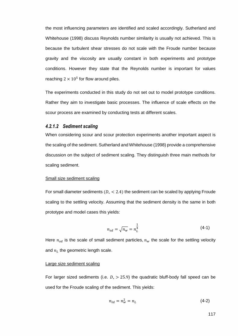
117

the most influencing parameters are identified and scaled accordingly. Sutherland and

Whitehouse (1998) discuss Reynolds number similarity is usually not achieved. This is

because the turbulent shear stresses do not scale with the Froude number because

gravity and the viscosity are usually constant in both experiments and prototype

conditions. However they state that the Reynolds number is important for values

reaching 2 × 105 for flow around piles.

The experiments conducted in this study do not set out to model prototype conditions.

Rather they aim to investigate basic processes. The influence of scale effects on the

scour process are examined by conducting tests at different scales.

4.2.1.2 Sediment scaling

When considering scour and scour protection experiments another important aspect is

the scaling of the sediment. Sutherland and Whitehouse (1998) provide a comprehensive

discussion on the subject of sediment scaling. They distinguish three main methods for

scaling sediment.

Small size sediment scaling

For small diameter sediments (𝐷∗ < 2.4) the sediment can be scaled by applying Froude

scaling to the settling velocity. Assuming that the sediment density is the same in both

prototype and model cases this yields:

𝑛𝑠𝑑 = √𝑛𝑤 = 𝑛𝐿

14 (4-1)

Here 𝑛𝑠𝑑 is the scale of small sediment particles, 𝑛𝑤 the scale for the settling velocity

and 𝑛𝐿 the geometric length scale.

Large size sediment scaling

For larger sized sediments (i.e. 𝐷∗ > 25.9) the quadratic bluff-body fall speed can be

used for the Froude scaling of the sediment. This yields:

𝑛𝑙𝑑 = 𝑛𝑤2 = 𝑛𝐿 (4-2)

118

Here 𝑛𝑙𝑑 is the scale for large sediments.

It should be noted that sediment scaling can be done using the Soulsby (1997) equation

for the settling velocity (𝑤𝑠) in conjunction with the Froude scaling. The benefit of the

Soulsby equation is that it is valid for the entire range of sediment sizes and does not

have discontinuities. The equation reads as:

𝑤𝑠 =𝜈

𝑑50(√10.362 + 1.049𝐷∗

3 − 10.36) (4-3)

Shields parameter scaling

One more way of scaling the sediment is by ensuring that the ratio 𝜃/𝜃𝑐𝑟𝑖𝑡 is the same

between the prototype and model. This ensures that the mode of sediment transport

(e.g. sheet flow or suspended load) is going to be the same, but the time scale of the

sediment transport may be affected.

An additional scaling consideration is the relative size of the sediment to structure

diameter. According to Chiew (1984) and Sheppard (2004) when the sediment size is

large relative to the structure the local pressure gradient induced by the structure on the

sediment particle decreases thus resulting in smaller scour depths. In clear water scour

this effect becomes negligible when:

𝑑50𝐷<1

50 (4-4)

An additional consideration regarding the sediment is the formation of ripples on the bed.

In laboratory conditions ripples tend to be relatively larger than in prototype conditions.

This problem arises because the spacing between the ripples is proportional to the

sediment size and sediments are not geometrically scaled in many physical models

(Sutherland and Whitehouse, 1998). There are two main concerns when ripples (i.e. live

bed scour regime) are formed in scour experiments:

119

a. Scour depths tend to be smaller. This is mainly because the ripples migrate

through the scour hole (incoming sediment flux) thus replenishing the local

sediment transport demand. This behaviour has been reported by numerous

authors among which are Melville (1984), Kawata and Tsuchiya (1988) and

Khalfin (2007).

b. The measurement of the scour depth becomes difficult as the ripples migrate

through the scour hole. This can introduce an error in the scour measurement in

the order of magnitude of the ripple height.

Given that the present study does not aim to model specific prototype conditions the

sediment was scaled according to the Shields method. The tests were conducted in the

clear water regime to minimize ripple effects which could make it difficult to determine

the equilibrium scour depth. In addition the size of the sand and structure were selected

in order to comply with Equation (4-4). This also avoids having large suspended

sediment quantities in the flow that could possibly damage the pumps.

4.2.2 Model effects

One of the most important model effects in flume experiments is the blockage effect.

Blockage effects arise when the width of the model is large relative to the flume width,

thus forcing the flow to accelerate. This is an important problem especially in scour tests

because it can potentially lead to deeper scour holes than what would be expected in

reality. Whitehouse (1998) suggests that blockage effects become negligible as long as

the following condition is met:

𝐴𝑚𝑜𝑑𝑒𝑙𝐴𝑓𝑙𝑜𝑤

<1

6 (4-5)

Here 𝐴𝑚𝑜𝑑𝑒𝑙 and 𝐴𝑓𝑙𝑜𝑤 are the cross-sectional area of the structure and the channel

projected to the flow. For the experiments conducted in this study the dimensions of the

structures were all selected in order to fulfill the above criterion.

An additional modelling consideration which arises when conducting scour experiments

is the time required to run an experiment in order to reach the equilibrium scour depth.

Defining in a consistent way the time to equilibrium scour is important for scour

120

experiments as it provides a method for stopping the test in a consistent manner thus

providing results that are comparable. Different approaches exist for stopping scour tests

(e.g. Melville and Chiew, 1999; Link, 2006; Fael et al, 2006) most of which are formulated

in a similar manner to the Melville and Chiew (1999) criterion:

∆𝑆

∆𝑡<0.05(𝐷 𝑜𝑟 𝐷𝑏𝑎𝑠𝑒)

∆𝑡 (4-6)

Here ∆𝑆 is the scour depth achieved over a time period ∆𝑡. These criteria have been

derived based on experimental studies that were conducted at different scales and thus

must be used with caution. In addition, they do not take into account possible effects the

geometry of a structure might have. Another way of defining the equilibrium scour depth

is proposed by Hoffmans and Verheij (1997) and Cardoso and Bettess (1999) which

suggest that the equilibrium scour depth can be assumed to be achieved once the slope

of the scour development curve has reached a value tending to zero when plotted in a

logarithmic plot. This definition is independent of scale effects and structure properties.

For these reasons this criterion was used to determine when to stop the scour tests

conducted in this study.

4.3 Description of set-up and the models for small scale scour tests

4.3.1 Flume and test set-up

The small scale scour experiments were conducted in the tidal flume in the Pat Kemp

Fluids Laboratory at University College London. The flume is 10m long, 0.3m in width

and 0.35m in height (see Figure 4-1). The flume operates as follows:

i. A pump delivers water from an underground sump to a constant head tank above

the flume.

ii. Water from the overhead tank delivers water to the flume inlet. The discharge is

then controlled through a series of valves.

iii. Water leaving the flume passes over a weir gate and then returns back to the

sump.

121

Figure 4-1: Layout of tidal flume: (a) top view; (b) side view.

122

The false bed was installed throughout the length of the flume in order to raise the bed

and enable the installation of a sand pit in the mid-section of the flume which would allow

the undertaking of scour experiments. In all tests the same type of sand used in the sand

pit section was glued on the false bed in order to minimize any additional turbulence

induced by the transition from one bed roughness to the other. In addition, the sand pit

was smoothed flush with the top of the false bed to ensure an easy transition of the flow

between the two sections. The roughened false bed also contributed to “tripping” the

boundary layer and ensuring that a rough boundary layer was present at the test section.

4.3.1.1 Sand installation and smoothing

The sand used for the experiments was pre-soaked in water for at least 10 days prior to

use in order to reduce the effects of air entrained within the sediment’s pores. The sand

was then carefully placed in the sand pit after the lower part of the foundation was

installed. Extra care was taken when the sand was placed in order to minimise air being

trapped. The following steps were followed each time the sand was introduced to the

sand pit:

1. The flume was filled 10-20mm above the false bed.

2. Sand was carefully placed in the sand pit with the use of a small trowel. Even

though the sand used in the tests was fairly uniform it was gently mixed when it

was placed in the sand pit. This allowed to have a more uniformly distributed

sand particles in the test section.

3. The sand bed was then flattened and smoothed with the use of a scraper which

was supported by a trolley system on levelled rails.

4. Excess sand was scraped to the false bed and then taken out of the flume.

4.3.1.2 Model Structures

The model structures were installed in the middle of the sand pit at a distance of 1m from

the end of the false bed and 0.15m from the side walls. A range of different geometries

were investigated in this test programme. These were; a monopile 45mm in diameter,

three conical based structures with side slopes of 45⁰, 60⁰ and 75⁰, a cylindrical base

123

structure and a truncated cylinder. The dimensions of the geometries are given in Figure

4-2.

Figure 4-2: Structure geometries for scour tests.

All structures were selected to have a base diameter of 45mm which is also the diameter

of the monopile to provide a basis for comparison. In addition, the stick-up height of the

base for the non-uniform cylindrical structures was also selected to have the same height

(i.e. 20mm) to provide a comparison of the effect this structural property has.

All models were made from black Polyvinyl Chloride (PVC) Rods which were trimmed

and then polished in order to obtain the required shape and to minimise possible

roughness effects. The models consisted of two parts:

A cylindrical foundation which had a diameter of 45mm (same diameter as the

base of the models) the top side of which was flush with the false bed. This

component was screwed to the base board of the flume and positioned in the

middle of the test section (see Figure 4-3 (a)). Then the sand was placed in the

sand pit and smoothed flush with the top of the cylindrical foundation.

The main part of the structure which was screwed to the foundation mentioned

above (see Figure 4-3 (b)). This enabled the initiation of the experiments after the

desired flow conditions were achieved.

124

Figure 4-3: Set-up of the structures for scour tests: (a) Lower part of model (buried under

the sand); (b) installation of model foundation on base.

4.3.2 Flow parameters

The purpose of the small scale experiments was to investigate the influence of different

hydraulic parameters on the scour around the structures presented in Figure 4-2. More

specifically the flow parameters tested in these experiments include the water depth, the

flow velocity, the sediment size and the structure geometry. This section provides the

rationale behind selecting the hydrodynamic forcing conditions for this test series.

4.3.2.1 Flow velocity

For this test series all velocities were designed to be in the clear water scour regime.

Experiments were conducted for different sediment mobility ratios (𝑈𝑐/𝑈𝑐𝑟) to investigate

the influence this parameter has on scour around complex structures in the clear water

regime. The critical flow velocity for the sediments used in the tests was determined in

accordance with both the Soulsby (1997) and Van Rijn (1984) methods, both of which

gave the same answer within two decimal points. Furthermore, prior to the scour tests

the critical velocity for the incipient motion of the sand was also determined

experimentally and found to be within 10% of the result given by the empirical equations.

The majority of the tests were conducted at a sediment mobility in the range of 0.73-1.

(a) (b)

125

This is because for these conditions scour depths tend to be the deepest for both live

and clear water scour regimes.

4.3.2.2 Flow depth

Two flow depths were examined in this test series. The first flow depth was selected as

165mm in order to yield a non-dimensional flow depth (ℎ/𝐷) of 3.7 which is above the

critical value of 3 after which the effects of the water depth become negligible according

Melville (2008). The second water depth was taken as 100mm in order to examine the

effect shallower flow depths have on the scour potential around complex structures. The

corresponding non-dimensional flow depth for these tests was 2.2 which is closer to the

corresponding value a GBF for a wind turbine would have in the North Sea which

corresponds to a flow depth of 35-40m approximately.

4.3.2.3 Sediment characteristics

Two types of sediments were used in the experiments. Given that the purpose of the

tests was to investigate the effect of the pressure gradient on scour the coarser sand

tests were conducted to investigate if the sand coarseness has an effect on the local

pressure field and thus on scour around complex structures. All existing knowledge

regarding the effect of 𝑑50/𝐷 has been conducted for scour around uniform cylinders,

which is not necessary applicable for more complex structures. These were selected in

order to avoid cohesion effects (i.e. 𝑑50 > 100𝜇𝑚). The two sands had a median size of

0.2mm (hereafter fine sand) and 0.6mm (hereafter coarse sand). The size of the

sediment was determined from sieving tests that were conducted on samples of the two

sediments in UCL’s Geotechnical laboratory (see Figure 4-4). Both sediments were fairly

uniformly graded with a geometrical standard deviation of 1.5 for the fine sand and 1.3

for the coarse sand.

126

Figure 4-4: Grain size distribution for the two sediment types used in the experiments.

The density of the sediment under wet and dry conditions was also determined for two

samples of the sand and are presented in the following table.

Table 4-1: Wet and dry density for both sediment types.

Sand type 𝑑50 (mm) Wet density (𝐾𝑔/𝑚3 ) Dry density (𝐾𝑔/𝑚3)

Fine sand 0.2 1601 1585

Coarse sand 0.6 1468 1490

As can be seen from Table 4-1 there is a small difference between the dry and wet

densities for each sand type which suggests that the sediments do not absorb significant

amount of water. The data also shows that the densities of the two sands differ by

approximately 5%.

4.3.3 Measurement techniques

This section provides a description of the measurement techniques used in the small

scale scour experiments. These include the measurement of the undisturbed flow

velocity and scour depth measurements.

4.3.3.1 Flow velocity measurements

As discussed in sections 1.3, 1.4 and 1.5 the undisturbed flow velocity is an important

influencing parameter for the scour potential around any structure. For this reason, the

127

velocity profile was measured at the location of the pile before it was screwed into place

prior to each set of experiments. The flow velocities for the scour experiments were

measured using Laser Doppler Velocimetry (LDV). The basic principle of operation of an

LDV uses two light beams to measure the flow velocity within a given control volume.

The two beams are obtained by splitting one beam in order to ensure coherence between

the two light sources. A transmitting optics lens focuses the beams at a specific location

at which they superpose (i.e. forma pattern of fringes). As particles in the water pass

through the fringes light is scattered. This scattered light is then collected by a

photodetector. The light received (which has a different frequency compared to the

original beam) is then analysed to determine the Doppler shift which is directly related to

the flow velocity of the passing particle (see Figure 4-5). The present LDV device was

capable of measuring the two orthogonal components of the flow velocity (u and w), i.e.

horizontal and vertical components respectively.

Figure 4-5: Schematic of LDV working principle

In order to measure the flow profile, the LDV was mounted on a traverse system capable

of moving in three dimensions outside the flume (see Figure 4-6). This allowed to make

precise point measurements of the flow without intruding the flow. The mean flow velocity

was then determined in accordance with the Soulsby (1997) method.

128

Figure 4-6: Traverse set-up with LDV

Further to the flow velocity for the scour experiments a set of flow measurements was

made in order to investigate the influence of the side walls on the flow across the channel

width. The test conditions for this preliminary experiment were:

Mean flow velocity (𝑈𝑐): 0.25m/s;

Flow depth (h): 165mm; and,

Nominal diameter of the sand comprising the bed: 0.6mm.

The mean velocity was selected to have relatively high magnitude in order to accentuate

any flow asymmetry across the channel width. The symmetry of the flow was then

checked by making detailed streamwise velocity measurements through the depth and

at positions across the channel. Flow measurements near the wall were not possible due

to the low concentration of seeding particles near the walls. Figure 4-7 shows the results

of these measurements.

129

Figure 4-7: Flow velocity in the cross-flow direction.

In this figure the vertical axis shows vertical distance from the bed, the horizontal axis

the distance across the flume (with negative values being closest to the far side of the

flume) and the colour map the flow velocity (u). It can be seen that the streamwise

velocity across the width of the test section is fairly uniform with a tendency to accelerate

along the far-side of the flume. The maximum variation near the water surface at the far-

side of the flume is 5% of the streamwise velocity at the centre. From the results of this

preliminary test it can be concluded that the flow is fairly homogeneous along the cross-

flow direction. Thus the mean flow along the centreline of the flume can be used to

characterise the flow in the channel.

4.3.3.2 Flow and scour depth measurements

The water depth for the experiments was determined using rulers which were attached

to the glass side-wall of the flume at different locations. The lower part of the rulers was

carefully positioned at the top of the sand bed and an average from all the rulers was

taken to determine the flow depth. This was done to account for the small flow changes

in the water depth due to the hydraulic gradient.

130

Several methods for the measurement of scour depth around structures are recorded in

the literature; Porter et al. (2014) provides a comprehensive review of the advantages

and disadvantages of each method. Because the main goal of these tests was to obtain

preliminary insights into the scour process for complex structures only the time series of

scour and the equilibrium scour depth were recorded.

For these tests the foundation (under the initial bed level) of the structure was marked at

5mm intervals. The scour depth readings were determined by visual observations and

through the use of time-lapse photography. At the initial stages of the scouring process

the scour depth was recorded every 10s. The frequency of measurements then reduced

as the scour hole developed and the scour rate reduced. The initial readings were

verified later through the time-lapse photographs which were acquired at intervals of 10s.

For these tests only the deepest scour point was recorded. This was located at an angle

ranging between 0⁰ and 90⁰ relative to flow direction.

4.3.4 Experimental programme

The purpose of the small scale experiments was to investigate the influence of the

structural geometry on the scour process around complex structural geometries (listed

in Figure 4-2). These structures were subjected to a series of different flow conditions to

investigate the influence they have on the scour potential.

All tests in this series were subject to a unidirectional current and were conducted in the

clear water scour regime. The influence of the bed material was investigated by

conducting tests with two types of sediment while keeping constant the sediment mobility

ratio (𝑈𝑐/𝑈𝑐𝑟). The effect of the flow depth on scour around such structures was also

investigated by conducting tests at two water depths which correspond to deep and

medium water depths.

All of the structures were subject to the same flow conditions in order to determine the

differences in the scour potential induced by each type. Given that the purpose of the

tests was to determine the maximum scour potential of the structures, the foundation

131

extended to the bottom of the sand pit. Error! Reference source not found. presents

the summary of the small scale scour experimental test programme.

Table 4-2: Small scale scour experiments programme.

No. Structure Type 𝑈𝑐 Flow Profile ℎ 𝐷 𝑜𝑟𝐷𝑏𝑎𝑠𝑒 𝑑50 𝑈𝑐𝑟 ℎ/𝐷𝑏𝑎𝑠𝑒* 𝑈𝑐/𝑈𝑐𝑟

(-) (-) (m/s) (-) (m) (mm) (mm

)

(m/s) (-) (-)

1.0 Truncated 0.195 Logarithmic 0.165 45 0.6 0.267 3.67 0.73

1.1 Cylindrical base 0.195 Logarithmic 0.165 45 0.6 0.267 3.67 0.73

1.2 45⁰ conical base 0.195 Logarithmic 0.165 45 0.6 0.267 3.67 0.73



1.5 Uniform cylinder 0.195 Logarithmic 0.165 45 0.6 0.267 3.67 0.73





1.10

0

75⁰ conical base 0.2 Logarithmic 0.165 45 0.2 0.227 3.67 0.88
































*For tests with uniform cylinders 𝐷𝑏𝑎𝑠𝑒 = 𝐷.

132

4.4 Description of set-up and the models for large scale scour

experiments

Scour experiments were conducted in a larger facility in order to:

Investigate scale effects on the scour process.

Examine the effect different flow profiles have on the scour process around

complex foundation geometries.

To collect data that can be used to develop a scour predictor.

This section will provide an overview of the set-up of the flume, the procedures followed

during the experiments, the measurement techniques and the list of experiments

conducted.


The large scale scour tests were conducted in the coastal flume which is located in the

Department of Mechanical Engineering at University College London. The flume has

dimensions of 20m × 1.2m × 1m (length × width × depth). The side walls and the base

of the flume were made of glass to allow visual observation and to facilitate non-intrusive

measurement equipment (e.g. Particle Image Velocimetry (PIV) and Laser Doppler

Velocimetry (LDV)). The flume is equipped with a set of active absorption piston wave

makers both ends, which allows the generation of waves from one end while the other

actively absorbs wave energy thus reducing wave reflections. Currents are generated

via recirculating pumps which are situated under the flume. The pumps are capable of

generating currents in two directions (forward and backward). The inlets and outlets of

the flow are located in front of each wave maker. Figure 4-8 provides a schematic of the

flume used in these experiments.

The large scale scour tests were conducted in the clear water scour regime under the

forcing of a unidirectional current. Due to the configuration of the flume it was not possible

to construct a false bed throughout the length of the flume. For this reason, the bed was

raised by means of a marine plywood ramp which hosted a sand pit in the centre of it.

The ramp consisted of the following components:

133

Sand pit in the centre of the flume. The sand pit had a depth of 25cm and was

filled with sand flush to the top of the apparatus.

False bed extending 2.2m on either side of the sand pit. The false bed was

roughened by gluing fine sand (same type of sand as used in the sand pit) on the

surface of the wooden surface. This was done to assist the development of the

turbulent boundary layer and to reduce the amount of turbulence induced by the

transition between the false bed and the sand pit surface.

Sand traps, to protect the pumps from the sediment. The sand traps were 30cm

gaps at the end of the false bed which were covered by perforated plates. This

allowed the majority of the sediment to settle into the trap and avoid getting

sucked into the pumps.

Ramps on either side of the false bed with a side slope of 1:6 (H : L). The slope

of the ramp was limited by the size of the flume and the location of flow inlet/outlet.

The entire apparatus described above was held in place by gluing the bottom parts to

the glass bed of the flume using silicone.

Flow straighteners (conditioners) were installed in front of the flow inlet. The purpose of

the conditioners was twofold:

To minimise the lateral and transverse turbulent velocity components induced by

the pump and inlet geometry.

To modify the flow velocity profile by changing the friction at different levels of the

flow.

The flow conditioner consisted of a number of rolled wire meshes which were installed

parallel to each other immediately after the flow inlet (see Figure 4-9). The configuration

of the meshes was then adjusted to achieve the desired flow profile.

The sand used in the experiments was placed in the sand pit and flattened following the

same procedure described in the section 4.3.1.1. Due to the size of the flume it was not

134

possible to have a trolley system to support the sand scraper. For this reason, the sand

bed surface was smoothed by the author who needed to be located in the flume.

Figure 4-8: Layout of costal flume in Mechanical Engineering Department

135

Figure 4-9: Image of the flow conditioner.

The foundation geometries tested in this flume were scaled-up models of the structures

used in the small scale tests. Given that scour tests at this scale had an expected

duration which was much larger than at the smaller scale, it was decided not to include

the 60⁰ conical base structure and the truncated cylinder in these tests. Figure 4-10

shows the dimensions of the structures used in these tests.

Figure 4-10: Large scale foundation geometries

136

The structures referred to in Figure 4-10 were then screwed onto the base component

which was already installed in the sand pit in a similar way to that shown in Figure 4-3

and described in section 4.3.1.2.

4.4.2 Flow parameters

All tests were conducted in the clear water scour regime with a sediment mobility ratio

(𝑈𝑐/𝑈𝑐𝑟) between 0.90 and 1. This flow condition (i.e. near critical flow velocity) was

selected because it was expected to induce the most severe scour depth. In addition,

two different flow profiles were tested:

a logarithmic flow profile, in order to examine possible scale effects compared to

the smaller scale experiments (Figure 4-11 a); and,

a non-logarithmic flow profile with the same flow flux as in the first set, for the

purpose of examining the possible effects of non-logarithmic flow profiles on the

scour process. The flow profile was altered through changes in the flow

straightener configuration in order to achieve a flow profile resembling one

subject to a wind stress at the surface (Figure 4-11 b).

Figure 4-11: Schematic of the flow profiles tested in these tests.

137

Three flow depths were tested in this set of experiments. The four geometries were

subjected to both logarithmic and non-logarithmic flow profiles with a depth of 350mm.

The purpose of these tests was to investigate the influence different profiles have on the

structures for a constant flow flux. To investigate the effect water depth has on complex

geometries in non-logarithmic flow profiles the 75⁰ conical base structure was further

tested at water depths of 350, 450 and 550mm. Finally, four structures were subjected

to a non-logarithmic flow profile at a depth of 550mm to further investigate the effect of

varying depth on the structures in such flow profiles.

The fine sediment used in these experiments was the same as the one used in the small

scale flume. The reader is referred to section 4.3.2.3 for further details regarding the

sediment distribution and density.

4.4.3 Measuring techniques

This section provides a description of the measurement techniques used in the large

scale experiments. The quantities measured during these tests include the flow velocity

and the scour depth around the structures.

4.4.3.1 Flow velocity measurement

For the large scale experiments the flow velocity was measured at the location of the pile

after the sand bed was smoothed and before the upper part of the pile was screwed into

place. Due to the width of the flume it was not possible to use the LDV to measure the

velocity at the centre of the flume due to the limited focal length of the LDV. For this

reason, the flow profile in the larger flume was measured using Acoustic Doppler

Velocimetry (ADV). For this test series a Vetrino+ ADV was used. As for the LDV the

ADV operates by the principle of the Doppler shift. The device sends out acoustic waves

with a specific frequency from the transmitter. These waves then reflect from the seeding

particles which are distributed in the flow and the acoustic receivers detect the change

in the frequency of the echoes. The Doppler shift detected by each sensor is proportional

to one of the three flow velocity components. Figure 4-12 provides a schematic of the

138

working principle of the ADV. Given that the ADV is an intrusive measuring instruments

the flow velocity was only measured prior to the initiation of the experiments to avoid it

interfering with flow.

The ADV was mounted on a vertical bar at the centre of the flume. The bar had holes at

1cm intervals which allowed precise vertical positioning within the water column. The

point measurements of the velocity were conducted for 3min in order to average out

effects of turbulence. The average flow velocity was then computed using the trapezoidal

rule described in Soulsby (1997).

Figure 4-12: Acoustic Doppler Velocimetry working principle (source: Sellar et al., 2015).

4.4.3.2 Flow and water depth measurement

In addition to measuring the time development and the equilibrium scour depth the large

scale experiments were intended to investigate the three dimensional characteristics of

the scour hole developed by the complex geometries. In these test the flow depth and

the time development of the scour was measured using time lapse photography in the

same manner outlined in section 4.3.3.2. The 3D shape of the equilibrium scour hole

was then measured using an echosounder device. The following paragraphs will

139

describe the principles of operation of the echosounder along with the general set-up of

the device used in the experiments.

The echosounder used in this study was a General Acoustics Ultralab UWS echosounder

which is capable of making point measurements. The device consisted of a sensor 30mm

in diameter and 50mm in height which needed to be in contact with the water surface in

order to make the measurements. The measuring frequency of the echosounder was

1MHz capable of measuring the water depth with a 1% accuracy with a maximum error

of 1mm. The operational range of the sensor is 1mm to 10m and the echo beam angle

was less than 3⁰.

To measure the morphology of the equilibrium scour hole, the echosounder was

mounted on a traverse system which was installed above the flume. This allowed the

sensor to move in the x (streamwise direction) and y (cross-flow direction) direction. For

the present tests the profiler was set-up to measure an area 700mm (x-direction) ×

690mm (y-direction) around the pile. The scour depth was then measured by taking point

measurements at 5mm intervals in the x and y direction. In order to reduce noise in the

depth measurements due to reflections of the echo beam off the structure the equilibrium

scour profile was taken after the structure was unscrewed from the base. For these

measurements the datum was taken as the bed elevation in front of the structure before

the initiation of the experiment. The scour depth was then determined by subtracting the

depth measurement of the echosounder from the datum level.

4.4.4 Experiment programme

The purpose of the large scale experiments was to gain insight to the effect the structural

scale and different flow profiles have on the scour development around complex

geometries. They were also designed to further investigate the effect of the water depth

has on the scour depth.

All tests were conducted under the forcing of a unidirectional current and were all in the

clear water flow regime. The sediment mobility number was selected to be between 0.9

140

and 1 as for these flow conditions the most severe scour depth is expected. Tests 3.1 to

3.4 were conducted under the forcing of a logarithmic flow profile and their main purpose

was to provide a dataset that would be compared to the small scale results from tests

2.2 to 2.6 which have similar non-dimensional values. Tests 3.5 to 3.8 were conducted

under the forcing of a non-logarithmic flow profile with the same flow flux and flow depth

as in tests 3.1 to 3.4. The purpose of these tests was to investigate the effect a different

flow profile has on the scour process. Tests 3.9 to 3.12 were conducted with a non-

logarithmic profile and a similar flow speed as in tests 3.5-3.8 but at a different flow depth.

This subset was designed to investigate the effect a change in flow depth has on the

scour process in non-logarithmic flow profiles. Finally, tests 3.12 to 3.14 were conducted

to investigate further the effect of the depth in such conditions. It should be noted that

test 3.14 was also conducted to investigate the repeatability of test 3.8. Table 4-3

presents a summary of the key flow parameters adopted in these tests.

Table 4-3: Large scale scour experiments programme.

No. Structure Type 𝑈𝑐 Flow Profile ℎ 𝐷 𝑜𝑟𝐷𝑏𝑎𝑠𝑒 𝑑50 𝑈𝑐𝑟 ℎ/𝐷𝑏𝑎𝑠𝑒* 𝑈𝑐/𝑈𝑐𝑟

(-) (-) (m/s) (-) (m) (mm) (mm) (m/s) (-) (-)

3.1 Monopile 0.245 logarithmic 0.35 200 0.2 0.253 1.75 0.97

3.2 Cylindrical base 0.245 logarithmic 0.35 200 0.2 0.253 1.75 0.97



3.5 Monopile 0.245 non-logarithmic 0.35 200 0.2 0.253 1.75 0.97

3.6 Cylindrical base 0.245 non-logarithmic 0.35 200 0.2 0.253 1.75 0.97

3.7 45⁰ conical base 0.245 non-logarithmic 0.35 200 0.2 0.253 1.75 0.97


3.9 Monopile 0.254 non-logarithmic 0.55 200 0.2 0.270 2.75 0.94

3.10 Cylindrical base 0.254 non-logarithmic 0.55 200 0.2 0.270 2.75 0.94





*For tests with Monopiles i.e. uniform cylinders, 𝐷𝑏𝑎𝑠𝑒 = 𝐷.

141

4.5 Description of set-up and the models for the pressure and flow

measurements near the structure


A number of small scale experiments were conducted in the flume described in section

4.3.1. In these tests the pressure distribution around a number of structures with both

uniform and non-uniform cylindrical geometries was measured using pressure

transducers. In addition, the flow field around each structure was measured for the same

conditions for which the pressure measurements were conducted. The setup of the flume

was similar to that of Figure 4-1 with the difference that the sand pit was removed and

replaced by a false bed. Figure 4-13 (a) shows the setup of the flume. For these

experiments, models of the structures shown in Figure 4-2 were generated using 3D

printing. In order to reduce costs, it was decided not to print the truncated cylinder. The

printed models of the structures were designed with tapping holes at different heights

along their face (see Figure 4-14), each of which led through internal tubes to the base

of the structure (Figure 4-13 and Figure 4-15). This allowed water through the structure

to the tubes connected to the pressure transducer at the bottom of the structure. The

internal tubes in the structures extended 10mm from the bottom of the model foundation

in order to allow enough space to connect them to acrylic tubes. The acrylic tubes were

then passed out of the flume via specially designed exit glands (Figure 4-13 (a) and

Figure 4-15) which finally connected to the transducer system.

142

(a) (a)

Figure 4-13: (a) Set up of the pressure measurement tests showing the acrylic tubes connecting to the pressure transducer units beneath the flume; (b) Image of 3D model; (c) cut through (from centreline) of model with tubes.

Figure 4-14: Location of pressure taps.

In order to allow the rotation of the structure which would enable the measurement of the

pressure field around it, a 45mm hole was opened through the false bed of the flume at

the mid-point of the test area. This allowed the structures to slip into the gap (all

(b) (c)

143

structures have a base diameter of 45mm) and provided stability with respect to the

overturning moments created by the flow and structure interaction. In addition, a

watertight seal was installed around the periphery of the hole in order to avoid flow

seeping through potential gaps which may be created between the structure and the

edge of the hole. The structures were then supported from the top via a support pin which

was held by an anchor clamp. The support system allowed the rotation of the entire

structure without the need to stop the flow.

Figure 4-15: Side view sketch of the lower part of the pressure measurement apparatus.

The present tests were designed to measure the pressure field around the GBF

foundation geometries tested in the scour experiments. The main objective of the tests

was to establish the range of validity of potential flow theory around these structures. For

this reason, only one flow condition was tested. For the present tests the false bed was

roughened by gluing 0.2mm sand across the surface of the flume’s bed. The undisturbed

flow velocity was measured at the location of the structure using an LDV.

144

Two types of flow measurements were conducted using the LDV for the same flow

conditions as for the pressure measurements:

Measurement of the two components of the flow velocity (u and w) along the

plane of symmetry of the structure.

Measurement of the two components of the flow velocity (u and w) in the volume

surrounding half of the structure (hereafter volumetric flow measurements).

Figures 2-10 and 2-11 show the points where the measurements where made in

the X-Y and X-Z planes respectively.

Figure 4-16: Flow field measurement points in the X-Y plane.

Figure 4-17: Flow field measurement points in the X-Z plane.

Flow direction

Flow direction

145

4.5.2 Measurement techniques

This section provides a description of the measuring equipment used for the current

tests. Given that all depth and velocity measurements were conducted using the same

equipment as for the small scale scour experiments the reader is redirected to section

4.3.3 for details about the set-up and working principles of the equipment. The present

section will therefore focus on the description of the pressure measurements.

4.5.2.1 Pressure measurement

The pressure transducer used for measuring the pressure around the structure was a

Honeywell 40PC001B2A series (see Figure 4-18). The present transducer is

temperature compensated and is regulated by its own internal amplifier. The transducer

has a sensor element of constant area which reacts to the pressure applied by the fluid

in the silicon tubes. The pressure of the fluid deflects the diaphragm inside the pressure

transducer which is then translated into a voltage output which is recorded by a data

logging system. The analogue voltage output is then translated into a pressure through

a linear calibration which was conducted prior to the experiments.

The tubes leading to the transducer were bled before the initiation of each test in order

to remove any air bubbles that may have been trapped in the tubing. In addition, the

connection of the transducer to the data-logger was conducted via coaxial cables instead

of regular copper cables. This provided a significant improvement in the signal quality

and sensitivity to the pressure forces.

Figure 4-18: Pressure transducer

146

4.5.3 Experimental programme

The present test programme was carried out under the forcing of a unidirectional current

with a mean flow velocity of 0.33m/s. This velocity was higher than the velocities tested

in the scour experiments listed in Tables Error! Reference source not found. Table 4-3

because they were below the operation range of the pressure sensor.

After the completion of the pressure measurements flow measurements were conducted

for the same undisturbed mean flow velocity. No flow measurements were conducted for

the 45⁰ conical base structure because it broke while being removed from the flume after

the pressure measurements. In addition, due to time constraints it was not possible to

conduct flow measurement around all the structures due to the time required for the tests.

For that reason, complete flow measurements were conducted only for the cylindrical

base, 75⁰ conical base and monopile. These structures represent the three different

types of geometries investigated in this study. Table 4-4 shows the experimental

programme for the flow conditions and the types of measurements conducted for this

test series.

Table 4-4: Flow and pressure measurement programme

Test Structure 𝑈𝑐 𝑑50 ℎ Pressure

measurement

Flow measurement

(plane of symmetry)

Flow measurement

(around structure)

(-) (-) (m/s) (mm) (m) (-) (-) (-)

4.1 Cylindrical

base

0.33 0.2 0.165

4.2 45⁰ conical

base

0.33 0.2 0.165

4.3 60⁰ conical

base

0.33 0.2 0.165

4.4 75⁰ conical

base

0.33 0.2 0.165

4.5 Uniform

cylinder

0.33 0.2 0.165

147

4.6 Database compilation for equilibrium scour prediction equation

A significant amount of equilibrium scour data has been published in the past. In this

study published data on equilibrium scour depths around both uniform and complex

cylindrical structures were selected in order to create an equilibrium scour prediction

equation for clearwater scour conditions. The decision to focus on the clearwater regime

was made in order to avoid data that were influenced by ripple formation upstream of the

structure, which would introduce additional sediment transport scale effects. A summary

of the sources and quantities of scour data is given in Table 4-5.

Table 4-5: Sources of data for scour prediction equation.

Data Source Number of data points

Complex geometries

Amini (2014) 6

Ataie-Ashtiani et al (2010) 8

Ferraro et al (2013) 10

Hoffmans and Verheij (1997) 1

Jannati et al (2015) 2

Melville and Raudkivi (1996) 7

Moreno et al (2015) 8

Parola et al (1996) 13

Simons et al (2009) 4

Whitehouse (2011) 2

Total complex geometries 61

Uniform Cylinders

Chabert and Engeldinger (1956) 85

Dey et al (1995) 18

Ettema (1980) 70

Ettema et al (2006) 5

Jain and Fischer (1979) 26

Melville (1997) 5

Melville and Chiew (1999) 12

Matutano et al (2013) 10

Shen et al (1969) 16

Sheppard and Miller (2006) 4

Sheppard et al (2004) 4

Yanmaz and Altinbilek (1991) 14

Total uniform cylinders 269

148

The data presented include scour tests that were conducted in the clearwater regime for

cohesionless sediments only. Data were included only if all relevant parameters were

presented in the publication. The aforementioned parameters include the median

sediment size, average flow velocity, the sediment geometric standard deviation, water

depth, structural dimensions and the time to equilibrium scour. Tests were discarded if:

They were not run for a sufficiently long period to achieve equilibrium scour.

According to Melville and Chiew (1999) this is the time required to reach a scour

depth in which the scour rate does not exceed 5% of the structure diameter in 24

hours; and,

The sediment geometric standard deviation (𝜎𝑔) was greater than 1.5. This was

done to avoid the effects of bed armouring.

In addition, for a limited number of structures that did not have a circular footprint the

equivalent diameter was determined and used. Only one field study is included in this

dataset (Matutano et al, 2013) even though there have been a large number of field

studies published. The majority of field studies were excluded for three reasons:

Field measurements tend to have time-varying flows which make it difficult to


In most cases, naturally occurring flows in tidal or alluvial environments are high,

thus forcing scour to occur in the live bed regime for at least part of the time. The

extensive bed formations developed upstream of the structure and the general

lowering of the bed would provide additional difficulty in generalising any

information; and,

In most cases it is not possible to monitor the scour development systematically

and, therefore, it is not possible to determine if the scour hole is fully developed.

149

5 Results for scour around complex structures

This chapter will present the results of the experimental study on scour around uniform

and non-uniform cylindrical structures. It will start with the results for the small scale

scour tests, then the large scale scour results followed by the pressure and flow

measurements around the same geometries.

5.1 Smaller scale scour results

This section will provide the results of tests listed in section (4.3.4). First the flow

conditions will be presented followed by the results for the time development of scour

and the equilibrium scour depths.

5.1.1 Flow conditions

For the small scale scour experiments. Flow profiles were measured at the location of

the pile before it was installed. Figure 5-1 (a) and (b) show the flow profiles for the 165mm

and 100mm water depth scour tests. The symbols correspond to the flow conditions

outlined in Table (4.1) and the lines show profile approximation for tidal currents

proposed by Soulsby (1990) and applied for the corresponding mean flow velocity. It can

be observed that the flow profiles for tests conducted with similar mean flow velocities

but with different bed roughness show good agreement. This behaviour may be

attributed to the fact that the flow has been developed at the location of the

measurement. Furthermore, it can be observed that all the measurements show a good

agreement with the prediction given by the Soulsby (1990) method. Therefore, it can be

safely stated that the present flow conditions resemble that of tidal currents.

150

Figure 5-1: Flow profiles for small scale scour tests: a) h=165mm and b) h=100mm.

5.1.2 Results

In this section the results from the small scale scour experiments will be presented.

5.1.2.1 Initiation of scour around complex geometries

During the initial stages of the scouring process the uniform cylinders showed a different

behaviour compared to the conical based structures. For the conical base structures, the

scour process initiates at the lee of the structure at an angle approximately 120° relative

to flow direction (see Figure 5-2). The deepest scour then gradually propagates towards

the upstream of the structure and reaches the leading face of the structure; the deepest

scour point then stabilizes at a location adjacent to the structure at an angle

approximately 45° relative to the flow direction. This point of initiation of scour agrees

with the findings of Tavouktsoglou et al. (2015) who found that the maximum

amplification of the bed shear stress occurs at the same location for all conical based

structures. This is consistent with the observations of Khalfin et al. (1983) who observed

that the maximum scour for some conical structures occurred at the lee of the structure.

This behaviour is also reported in Petersen (2014) who examined the behaviour of edge

scour around protected piles with the difference that the maximum scour depth did not

move towards the front of the scour protection scheme.

a) b)

151

This behaviour can be explained by the presence of the conical base (which is composed

of a cone imposed onto a cylinder) which effectively weakens the horseshoe vortex at

the initial stages of the scour process (as will be shown in section 5.3.3), thus making

the scour process vortex-shedding dominated. Once the scour reaches the leading face

of the structure then the horseshoe vortex gains more strength as a result of the greater

depth over which it has to act, therefore making it a horseshoe vortex-dominated process

which explains the shift of the maximum depth of scour to the same location where it

occurs for a monopile.

Figure 5-2: (a) Initiation of scour at 45° conical base structure, (b) bed shear stress amplification contour map for same structure; flow direction from left to right.

5.1.2.2 Temporal evolution of scour

In this section the scour development around the structures detailed in section (4.3.4)

are presented. The results for each flow condition will be presented in one graph to

demonstrate the effects of geometry on the scour development.

Figure 5-3 presents the results for tests 1.0-1.5. The tests were conducted at a flow depth

of 165mm with a sediment mobility ratio of 0.73 with 𝐷50 = 0.6mm. The value of 𝑈/𝑈𝑐 is

relatively small but the purpose of this test was to examine the behaviour of the scour

development when the current strength is not large. In general, the scour development

follows a similar trend to that expected when plotting the data on a log scale (Figure 2-

26). The monopile structure tends to start off with a scour rate similar to the other

structures then log scale gradient increases. This behaviour might be attributed to the

increasing strength of the horseshoe vortex as the scour hole deepens. The 75⁰ and 60⁰

(a) (b)

152

conical based structures follow the expected scour development trend as they reach the

development phase (steeper slope in the graph) early in the tests. The behaviour for the

45⁰ conical base structure and the cylindrical base structure is different to the

aforementioned structures. More specifically, the data show that it takes some time for

the scour to enter the development phase. This behaviour might be attributed to the

limited effect the shaft of the structure has on the scour process due to sheltering of the

bed provided by base of the structure. Finally, the truncated cylinder shows minimal

scouring due to the limited effect it has on the flow.

Figure 5-3: Time development of scour for tests 1.0-1.5 (ℎ = 0.165𝑚, 𝑑50 = 0.6𝑚𝑚 𝑎𝑛𝑑 𝑈𝑐/𝑈𝑐𝑟 = 0.73).

Figure 5-4 shows the results for tests 1.6-1.11. The present tests were conducted for the

same flow depth as in the previous case and 𝑈𝑐/𝑈𝑐𝑟 = 0.88 over a bed comprised of

sediment with 𝑑50 = 0.2mm. It can be observed that the development trends for all the

structures with the exception of the truncated cylinder follow a more linear behaviour (in

the log-scale) with the structures entering the development phase early on in the

experiment. In the case of the truncated cylinder the scour rate is considerably smaller

compared to the other structures in the initial stages. The scour rate for this structure

starts to increase for a scour depth ≳ 0.2𝑆/𝐷𝑏𝑎𝑠𝑒, which is the same non-dimensional

153

depth at which the cylindrical and 45⁰ conical as seen in Figure 5-3. Furthermore, it can

be observed that the rate of scour (i.e. slope of the graph) is the same for all the

structures except for the truncated cylinder.


Figure 5-5 shows the results for tests 1.12-1.17 which were conducted for a flow depth

of 165mm, sediment mobility ratio of 0.98 and a sediment median size of 0.2mm. In these

tests all of the structures tend to follow a straight trend in the logarithmic plot. There is a

clear increase in the scour rate for all structures compared to the previous set of tests

(tests 1.6-1.11). This increase is in the order of 10%. Interestingly, for this flow condition

the scour development for the 45⁰ and 60⁰ conical base structures is almost identical to

each other.

154


The following graph (Figure 5-6) shows the results for tests 1.18-1.21. These tests were

conducted for similar flow conditions as in 1.6-1.11 with the exception of the bed material

which in these tests had 𝐷50 = 0.6mm. The purpose of these tests was to examine the

effect the sediment size has on the scour process. As can be seen in the figure the scour

development follows the same trend for all the structures as the ones in Figure 5-4. An

exception to this observation is the truncated cylinder which has a slower scouring rate

under the same flow conditions. This behaviour might be effected by 𝑑50/𝐷 scaling

effects as described in section (4.2). Considering that this rule has been derived for

monopiles extending to the water surface it can be expect that scaling issues would arise

for an even smaller ratio of 𝑑50/𝐷 in the case of truncated cylinders because the pressure

field around it is weaker and thus any scaling issue would be more pronounced. This

could explain the smaller scour rate and equilibrium depths observed for this test.

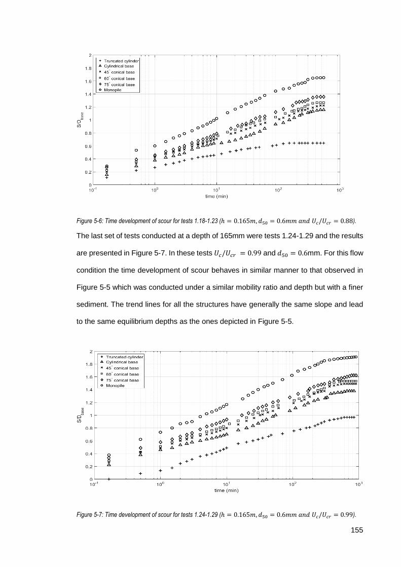
155


The last set of tests conducted at a depth of 165mm were tests 1.24-1.29 and the results

are presented in Figure 5-7. In these tests 𝑈𝑐/𝑈𝑐𝑟 = 0.99 and 𝑑50 = 0.6mm. For this flow

condition the time development of scour behaves in similar manner to that observed in

Figure 5-5 which was conducted under a similar mobility ratio and depth but with a finer

sediment. The trend lines for all the structures have generally the same slope and lead

to the same equilibrium depths as the ones depicted in Figure 5-5.


156

Two sets of scour experiments were conducted at a smaller water depth (ℎ=100mm) to

investigate the effect this parameter has on scour. Tests 2.1-2.6 (Figure 5-8) were

conducted for a flow velocity of 0.2m/s with a sediment size of 0.2mm which leads to a

sediment mobility ratio of 0.93. Tests 2.7-2.12 (Figure 5-9) were undertaken at flow a

velocity of 0.19m/s with 𝑑50 = 0.6mm which yields a 𝑈𝑐/𝑈𝑐𝑟 =0.78. In both graphs it can

be observed that the scour rate and equilibrium scour depths for all structures except for

the monopile are larger than the ones produced for the same sediment mobility ratio at

a larger depth. At first glance this contradicts the generally accepted rule for cylinders

which suggests that a decreasing flow depth yields smaller scour depths. In the case of

the non-uniform cylindrical structures a smaller flow depth forces a larger portion of the

flow to interact with the lower part of the structure which in the case of these tests is

wider. This phenomenon is linked to the local increase in the pressure gradient due to

the flow and structure interaction and will be further discussed in the next chapter. This

process may explain this increase in the scour rate and equilibrium depth.


157


Figure 5-10 demonstrates the influence of the ratio 𝑈𝑐/𝑈𝑐𝑟 on the scour development

for three representative structures tested in this study (cylindrical base, 60° conical base

and uniform cylinder). It can be observed that an increase in the mobility ratio yields an

increase in the rate of scour and equilibrium scour depth which is in accordance with the

findings of Breusers et al., (1977) for uniform cylinders.

The present data also show that for the cases where 𝑈𝑐/𝑈𝑐𝑟 is constant (or has a similar

value) an apparent deceleration in the scour rate is observed as it approaches its

equilibrium stage for the cases where the coarser bed material is used. This deceleration

effect is reduced as the blockage induced by the structure increases and as the mobility

ratio increases. It is noted that according to Raudkivi and Ettema (1983) the effects of

bed armouring are minimal as the geometric standard deviation of the sediments

presented here are minimal since the 𝜎𝑔 for both the sands is smaller than 1.5.

Figure 5-10 also shows the effect the side slope of the structure has on the development

of scour. It can be observed that as the side slope of a structure increases, the rate of

158

scour also increases which is a result of the local amplification of the pressure gradient

due to the increased obstruction.

Figure 5-10: Influence of 𝑈𝑐/𝑈𝑐𝑟 on scour development for three different structure geometries.

The present experiments also suggest that the geometry of the foundation plays an

important role with regards to the shape of the scour hole. Figure 5-11 shows that for a

cylindrical base structure at low mobility ratios (𝑈𝑐/𝑈𝑐𝑟 < 0.8) the scour hole did not

extend around the periphery of the structure. The scour process eroded sediment from

the upstream face of the structure and deposited it at the lee. This behaviour has also

been reported by Briaud et al. (2004) and Ataie-Ashtiani et al. (2010) and is further

supported by the flow measurements that will be presented in section 5.3.3.4. The flow

measurements show that a clockwise circulation cell is present at the lee of the structure

which brings sediment from further downstream near the edge of the base.

Consequently, it can be stated that the shape of the footing plays an important role which

should be considered when investigating scour phenomena and particularly scour

protection schemes.

159

Figure 5-11: Observed scour depth at cylindrical based pier before under-cutting the base cylinder (ℎ =0.165𝑚, 𝑑50 = 0.6𝑚𝑚 𝑎𝑛𝑑 𝑈𝑐/𝑈𝑐𝑟 = 0.88).

5.1.2.3 Equilibrium scour depth

This section will present the results for the equilibrium scour depths for the small scale

(i.e. smaller than 1:100) experiments. First will be discussed the importance of the non-

dimensionalising parameter, then the influence of the geometry and the water depth on

the equilibrium scour depth. Table 5-1 presents the scour depths for each tests.

Table 5-1: Equilibrium scour depth for small scale scour experiments.

Test No 𝑆/𝐷𝑏𝑎𝑠𝑒 Test No 𝑆/𝐷𝑏𝑎𝑠𝑒 Test No 𝑆/𝐷𝑏𝑎𝑠𝑒 Test No 𝑆/𝐷𝑏𝑎𝑠𝑒

1.0 0.1 1.11 1.69 1.22 1.36 2.4 1.42

1.1 0.59 1.12 1.02 1.23 1.65 2.5 1.49

1.2 0.87 1.13 1.38 1.24 0.97 2.6 1.69

1.3 0.95 1.14 1.49 1.25 1.38 2.7 0.62

1.4 1.12 1.15 1.52 1.26 1.49 2.8 0.9

1.5 1.43 1.16 1.64 1.27 1.53 2.9 1.16

1.6 0.73 1.17 2 1.28 1.62 2.10 1.22

1.7 1.16 1.18 0.64 1.29 1.93 2.11 1.25

1.8 1.23 1.19 1.16 2.1 0.87 2.12 1.49

1.9 1.31 1.2 1.22 2.2 1.26

1.10 1.38 1.21 1.27 2.3 1.36

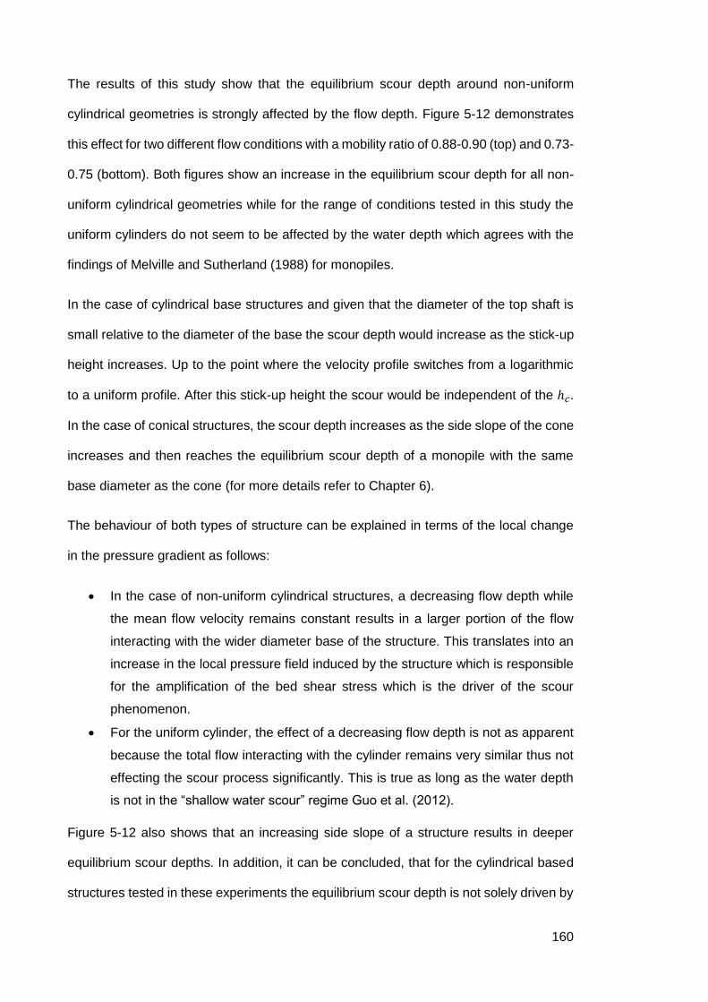
160

The results of this study show that the equilibrium scour depth around non-uniform

cylindrical geometries is strongly affected by the flow depth. Figure 5-12 demonstrates

this effect for two different flow conditions with a mobility ratio of 0.88-0.90 (top) and 0.73-

0.75 (bottom). Both figures show an increase in the equilibrium scour depth for all non-

uniform cylindrical geometries while for the range of conditions tested in this study the

uniform cylinders do not seem to be affected by the water depth which agrees with the

findings of Melville and Sutherland (1988) for monopiles.

In the case of cylindrical base structures and given that the diameter of the top shaft is

small relative to the diameter of the base the scour depth would increase as the stick-up

height increases. Up to the point where the velocity profile switches from a logarithmic

to a uniform profile. After this stick-up height the scour would be independent of the ℎ𝑐.

In the case of conical structures, the scour depth increases as the side slope of the cone

increases and then reaches the equilibrium scour depth of a monopile with the same

base diameter as the cone (for more details refer to Chapter 6).

The behaviour of both types of structure can be explained in terms of the local change

in the pressure gradient as follows:

In the case of non-uniform cylindrical structures, a decreasing flow depth while

the mean flow velocity remains constant results in a larger portion of the flow

interacting with the wider diameter base of the structure. This translates into an

increase in the local pressure field induced by the structure which is responsible

for the amplification of the bed shear stress which is the driver of the scour

phenomenon.

For the uniform cylinder, the effect of a decreasing flow depth is not as apparent

because the total flow interacting with the cylinder remains very similar thus not

effecting the scour process significantly. This is true as long as the water depth

is not in the “shallow water scour” regime Guo et al. (2012).

Figure 5-12 also shows that an increasing side slope of a structure results in deeper

equilibrium scour depths. In addition, it can be concluded, that for the cylindrical based

structures tested in these experiments the equilibrium scour depth is not solely driven by

161

the cylindrical footing. Comparison between the values of equilibrium scour depth of the

truncated cylinder and cylindrical based structure show that the latter structure type

yields equilibrium scour depths which are 7 % and 36% greater than that of the truncated

cylinder with the same height of emergence, depending on the given flow conditions and

sediment type. The data suggest that the difference between the equilibrium scour of the

two structures increases as the water depth increases, which is in line with the notion of

increased pressure gradients. These points suggest that the scouring process is not

solely dependent on the horseshoe vortex formed by the footing of the structure, but is

also influenced by the shaft of the structure which contributes to the increase of the

pressure gradient and therefore increases the equilibrium scour depth.

The results also demonstrate that the equivalent diameter is not effective in describing

the equilibrium scour depth for the structure geometries tested in this study. Figure 5-12

and Figure 5-13 present the same results with the difference being that in the first the

scour depth in non-dimensionalised by the diameter of the base (𝐷𝑏𝑎𝑠𝑒) and in the

second by the equivalent diameter as proposed by Coleman (2005). It can be seen that

non-dimensionalising the equilibrium scour depth with the equivalent diameter yields

unrealistically high non-dimensional scour depths in most cases and particularly in the

case of submerged/truncated cylinders.

Given that the scale at which these experiments have been conducted is small, it is

expected that the non-dimensional scour depths included in this study may be subject to

scale effects. According to Schlichting (1968) the size of the boundary layer is

proportional to 1/ln(Re) which means that the overall turbulence induced by the flow

structure interaction would decrease as the Reynolds number increases. In addition,

Achenbach (1968) showed that an increasing 𝑅𝑒𝐷 forces the separation point on the face

of the structure to shift further to lee of the pile which would also result in a decrease in

the sediment transport capacity of the lee wake vortices and thus decrease the overall

162

scour potential. This shows that 𝑅𝑒𝐷 could account for some scale effects that result in

smaller scour depths for larger scale structures.

Figure 5-12: Influence of water depth on equilibrium scour depth for different structure types (non-dimensionalised by base diameter of the structure).

Figure 5-13: Influence of water depth on equilibrium scour depth for different structure types (non-dimensionalised by equivalent diameter according to Coleman, 2005).

5.1.2.4 Repeatability of tests

This section will deal with the repeatability of the small scale scour experiments. The

repeatability of a physical tests is important for two reasons:

It demonstrates that the test conditions can be repeated and that the outcome of

the tests is not subject to large variations

163

It can provide a measure of the error in the measurement.

Due to the long duration of the tests, in this study it was decided not to repeat certain

tests. Instead some tests are compared with the results of another author who conducted

scour experiments in the same flume using the same sediments. The advantage of this

practice is that the data used for the comparison are independent of errors that may

occur due to the procedures and measuring techniques used in the current study.

Test 1.5 which was conducted for a uniform cylinder of 𝐷=45mm at a flow velocity of

0.2m/s, a flow depth of 0.165m and a sediment size of 𝑑50=0.6mm. This test was

compared with results from Porter (2016) who conducted scour tests in the same flume

with the same sediment for a uniform cylinder of 𝐷=40mm, a flow velocity of 0.19m/s

and the same flow depth. Figure 5-14 provides the comparison between the two tests.

As can be observed, the scour evolution curves for the tests show good agreement. The

largest discrepancy between the two tests is 5% 𝑆/𝐷. This occurs as the scour process

reaches the equilibrium stage. Given the slight differences in pile diameter and flow

velocity this is reasonable.

Figure 5-15 presents the results from the second comparison between the test 1.11

which corresponds to the monopile with D=45mm, Uc = 0.20m/s and d50 = 0.2mm and

an equivalent test of Porter (2016) which was conducted for D=40mm, Uc = 0.19m/s and

d50 = 0.2mm. The comparison between the two time development curves is similar to

that shown in Figure 5-14. The maximum error between the two data sets is 5.5% 𝑆/𝐷.

The maximum error occurrs at the equilibrium phase of the scour process which

coincides with the finding of the previous figure. Given that the velocity and the pile

diameter are slightly smaller in the experiment of Porter (2016) this behaviour is

expected.

164

Figure 5-14: Comparison of test 1.5 with Porter (2016) with D=40mm, 𝑈𝑐 = 0.19𝑚/𝑠 and 𝑑50 = 0.6𝑚𝑚.

Figure 5-15: Comparison of test 1.11 with Porter (2016) with D=40mm, 𝑈𝑐 = 0.19𝑚/𝑠 and 𝑑50 = 0.2𝑚𝑚 .

Concluding, the comparisons reveal that the maximum difference between the two pairs

of tests is 0.055 𝑆/𝐷 which can be taken as the uncertainty of the tests. The comparisons

also show that the rate of scour in the present study follows the same behaviour as in

165

Porter (2016) which can lead to the conclusion that the tests in this study can be repeated

by other researchers.

5.2 Large scale scour results

This section will provide the results for the tests detailed in the section (4.4.4). First the

flow conditions will be presented followed by the results for the time development of

scour and the equilibrium scour depths. Finally, the section will conclude with a

discussion on the repeatability of the tests.

5.2.1 Flow conditions

This section presents the unidirectional flow conditions under which the large scale scour

tests were carried out. One of the main aims of these tests was to investigate the effect

of non-logarithmic flow profiles on the scour process. Such flow profiles may be present

in locations where large lateral wind loads are expected such as the locations where

offshore wind farms are situated. In these locations the wind load effectively produces a

wind driven shear flow on top of the existing logarithmic flow (Davies and Lawrence,

1994) creating a flow profile similar to that of Figure 2-11 (b). To create these flow

profiles, flow straighteners were used to alter the flow profiles and the resulting flow

profiles are presented in Figure 5-16 (a) and (b). Figure 5-16 (a) shows the measured

logarithmic profile and the tidal flow prediction of Soulsby (1990) for the same mean flow

velocity. Figure 5-16 (b) shows the measured flow profiles for the non-logarithmic flow

profiles which were conducted at 3 different flow depths. All four flow profiles yielded a

mean flow velocity of 0.25m/s which allowed the comparison of the results while keeping

the flow flux constant.

The measured flow profile in Figure 5-16 (a) and the prediction of Soulsby (1990) shows

good agreement which can allow us to conclude that the present flow condition is

representative of a tidal flow. The measurements shown in Figure 5-16 (b) for non-

logarithmic profiles also show a resemblance to the behaviour captured by the model of

166

Holmedal and Myrhaug (2013) who calculated and verified the flow profile of a combined

tidal and wind driven flow in the Celtic Sea (given in Figure 5-17).

Figure 5-16: Flow profiles for large scale scour tests: a) logarithmic flow profile and b) non-logarithmic flow profiles.

Figure 5-17: Velocity profiles when the wind is opposing the tide (left) and when the wind is following the tide (Source: Holmedal and Myrhaug, 2013).

a) b)

167

5.2.2 Results

This section will present the results of the larger scale experiments. The section will first

present the findings regarding the temporal evolution of scour around the structures and

then the equilibrium scour depths. The section will then conclude with a discussion on

the repeatability of the tests.

5.2.2.1 Temporal evolution of scour

Figure 5-18 presents the results for tests 3.1-3.4 which correspond to a logarithmic flow

profile at a water depth of 350mm and 𝑈𝑐/𝑈𝑐𝑟=0.94. As was the case for the small scale

test the data behave in accordance with the time development profile described in

Hoffmans and Verheij (1997), with the scour developing rapidly at the initial stages and

then slowing down later into the tests. The scour rates for the three complex geometries

(i.e. cylindrical base, 45⁰ and 75⁰ conical base structures) are similar at the initial stages

of the scour process. The time development then decelerates in the later stages of the

tests with the smaller structures reaching the equilibrium stage sooner than the larger

ones. Interestingly, the scour process for the monopile starts off much more rapidly than

the other cases and then decelerates, reaching a scour rate similar to the other structures

(at t=1min). The scour then accelerates once again approximately at t=20min. This

behaviour is also recorded in the smaller scale tests and is attributed to the gain in

strength of the horseshoe vortex with an increasing local depth. When comparing the

results of these experiments with those of small scale tests it can be observed that the

time scale of the scour process is approximately 3-4 times slower for the larger scale

experiments. This is in accordance with the scour evolution equation presented in

Equation (2-48). According to equations (2-49) and (2-50) the time scale of scour around

a cylinder in a unidirectional current is 𝑇 𝐷. Given that the scale of the structures has

increased by a factor of 4 between the two sets of experiments this increase in the time

scale of scour is reasonable. The present data also show that the same time scaling also

applies to the complex geometries.

168

Figure 5-18: Temporal evolution of scour for a logarithmic flow profile, h=350mm.

Figure 5-19 presents the results for tests 3.5 to 3.8 which were conducted under the

forcing of a non-logarithmic profile and for similar flow conditions as the results presented

in Figure 5-18. The results reveal that the scour development for the monopile follows

very similar path to the logarithmic case (see Figure 5-18). In the case on the non-uniform

structure geometries (i.e. cylindrical base, 45⁰ and 75⁰ conical base structures) the rate

of scour is significantly reduced, by a factor of 50% approximately. This behaviour can

be explained by the change in the spatial distribution of the flow velocity through the

water column. With the non-logarithmic profile smaller flow velocities are present near to

the bed where the structure has the largest diameter. This leads to the local amplification

in the adverse pressure gradient being smaller.

169

Figure 5-19: Temporal evolution of scour for non-logarithmic flow profile, h=350mm

Figure 5-20 shows the results for the scour development for the four geometries under

the forcing of a non-logarithmic flow profile for a flow flux similar to tests 3.5-3.8 with the

difference that the flow depth has been increased to 550mm. The behavior of the

monopile structure follows a similar trend to the two previously presented results. This

behavior is expected as the total flow flux is constant and the change in the adverse

pressure gradient is not very great compared to the other cases. Observing the

behaviour of the remaining non-uniform geometries it can be seen that the overall scour

rate is further reduced compared to Figure 5-19. This can also be explained by the

increase in the water depth. The flow profile in this case shows that there is a reduction

of the velocity near the bed compared to the previous case (Tests: 3.5-3.8) which means

that the local amplification of the pressure field near the bed will be smaller; thus the

scour rate should also be smaller.

To further examine the effect water depth has on the scour process the 75⁰ conical base

structure was tested under similar velocities (i.e. 𝑈𝑐/𝑈𝑐𝑟 ~0.94) at water depths of

350mm, 450mm and 550mm. The results reveal that the scour rate and equilibrium scour

170

depth reduce as the depth increases which is in line with the finding of tests 3.5-3.12.

These findings show that there is an apparent link between scour rate, the flow profile

and the shape of the structure which will be examined in chapter 6.

Figure 5-20: Temporal evolution of scour for non-logarithmic flow profile, h=550mm.

Figure 5-21: Temporal evolution of scour for the 75deg conical base structure with non-logarithmic flow profile, h=350mm, h=450mm and h=550mm.

171

5.2.2.2 Equilibrium scour depths

This section will present the equilibrium scour depths for the large scale experiments.

For these tests full profile measurements of the scour hole were taken using the

echosounder. This made it possible to show contour maps of the equilibrium scour hole.

Table 5-1 presents the equilibrium scour depth for each test which is taken as the

deepest point of scour at the time at which the test was stopped.

Table 5-2: Equilibrium scour depth for large scale experiments.

Test No 𝑆/𝐷𝑏𝑎𝑠𝑒 Test No 𝑆/𝐷𝑏𝑎𝑠𝑒 Test No 𝑆/𝐷𝑏𝑎𝑠𝑒 Test No 𝑆/𝐷𝑏𝑎𝑠𝑒

3.1 1.17 3.5 1.17 3.9 1.22 3.13 0.54

3.2 0.72 3.6 0.57 3.10 0.32 3.14 0.72

3.3 0.78 3.7 0.61 3.11 0.41

3.4 0.84 3.8 0.71 3.12 0.51

Figure 5-22 presents the contour maps of the equilibrium scour depth for Tests 3.1-3.4

where scour below the initial bed level is given as negative values. These show that the

maximum scour occurs at an angle 45⁰-90⁰ relative to flow direction. This coincides with

numerous studies on scour (Hjorth, 1975 and Sumer et al., 1994) and with potential flow

theory which suggests that the maximum amplification of the pressure gradient occurs

at 45⁰. An interesting observation is that in the case of the monopile the scour hole

becomes significantly shallower at the downstream side of the scour hole which is a

common scour pattern in shallow water scour according to (Amini et al., 2011). In the

case of the complex structures though, the scour hole tends to become shallower at an

angle of 130⁰ relative to the flow direction and deepens once again as we approach an

angle of 180⁰. This effect may be explained by the non-uniform cross-sectional shape of

the structure which effectively reduces the size of the horseshoe vortex. The reduced

size of the horseshoe vortex makes the interaction of the contracted flow with the lee

wake vortices stronger and thus the scour deeper at this location. Furthermore, it can be

observed that the extent of the scour hole increases as the cross-sectional area of the

172

structure increases. The monopile induces the widest scour hole and the cylindrical base

structure the narrowest.

Figure 5-22: Equilibrium scour depth profiles for Tests 3-1-3.4 at h=350mm and a logarithmic flow profile (flow from

bottom): a) Monopile; b) Cylindrical base; c) 45⁰ conical base structure; and d) 75⁰ conical base structure.

Another interesting observation is the slope of the scour hole upstream and downstream

of the structures (see Appendix B for figure). The upstream slope of the scour hole for

all structures ranges between 38⁰ and 40⁰ which for the specific sediment falls within the

expected values of the angle of repose for submerged sediments (Miedema, 2014) but

is higher than the angle of repose of loose sand reported by Sumer and Fredsøe (2002).

The steep slopes may also be explained by the presence of a strong horseshoe vortex

in the scour hole which effectively helps the steep slope not to collapse. There is a

a) b)

c) d)

Monopile

Cylindrical base

75⁰ conical base

45⁰ conical base

173

significant change in the behavior of the downstream slope of the scour hole with

recorded slopes ranging between 9⁰ and 15⁰ which significantly smaller to those reported

in literature (Sumer and Fredsøe, 2002). There is no clear correlation between the

downstream slope and the structure type.

The scour pattern for tests 3.5-3.8 are presented in Figure 5-23. The flow conditions are

the same as in Figure 5-22 with the difference that for these tests the profile is non-

logarithmic. Comparison between the two sets of figures (Figure 5-22 and Figure 5-23)

shows that the scour patterns for each structure have qualitative similarities. The scour

hole becomes shallower at the downstream end of the monopile, while for the complex

structures there is a secondary depression behind the structure. Under the forcing of the

non-logarithmic flow profile it can be observed that the point of deepest scour shifts

further to the lee in the case of the monopile. This behaviour may be attributed:

To the weaker horseshoe vortex due to the smaller flow velocities near the bed

which reduces the amplification upstream of the pile.

To the stronger vortex shedding induced by the higher velocity near the surface

of the flow.

Further comparison between the two figures reveals that the maximum scour depth in

the case of the non-logarithmic flow profile is significantly reduced for the complex

structures. This agrees with the notion of reduced pressure gradients due to the change

in the flow profile.

For this flow condition there is evidence that there is a link between the structure and the

average slope upstream and downstream of the structure (also see Appendix B). Table

5-3 shows that as the size of the structure decreases both the upstream and downstream

slopes of the scour hole become milder. This finding might be linked to the intensity of

the horseshoe vortex which weakens as the structures decrease in size and thus is not

able to maintain the steep slopes. This can also explain the evidence of avalanching

upstream of the complex structure that can be seen in Appendix B.

174

Table 5-3: Upstream and downstream slopes of the scour slope for tests 3.5-3.8.

Test Structure 𝜑𝑢𝑝 (⁰) 𝜑𝑑𝑜𝑤𝑛 (⁰)

3.5 Monopile 45 42

3.8 75⁰ conical base 40 24

3.7 45⁰ conical base 36 15

3.6 Cylindrical base 30 12

Figure 5-23: Equilibrium scour depth profiles for Tests 3-5-3.8 at h=350mm and a non-logarithmic flow profile (flow from bottom to up): a) Monopile; b) Cylindrical base; c) 45⁰ conical base structure; and d) 75⁰ conical base structure.

The 3D scour profiles for tests 3.9-3.12 with a deeper flow depth are presented in Figure

5-24. The small lateral extent of the scour hole in front of the structures allowed the

measurement of the deposition pattern behind them. It can be observed that although

a) b)

c) d)

Monopile

Cylindrical base

75⁰ conical base

45⁰ conical base

175

the scour pattern is qualitatively similar to the other cases the width of the scour holes is

significantly smaller. This behaviour may be linked to the non-logarithmic flow profile

which has even lower near-bed velocity compared to the two previous cases. This can

translate to a weaker horseshoe vortex and thus scour depths. An exception to this

observation is the 45⁰ conical base structure which has a very asymmetric scour pattern.

This deviation to the scour pattern may be attributed to the lateral seiche which was

observed during the specific test. The causes of this are not clear but a possible

explanation might be the interaction between the water surface disturbance caused by

the lee wake vortices and the sidewalls of the flume. The figures also reveal that there

are secondary scour holes radiating away from the structure at an angle of 135⁰ to 150⁰

relative to the flow direction which are a consequence of the lee wake vortex shedding.

These secondary scour holes become larger in diameter for structures with a larger

cross-sectional area. This is because the diameter of the structure near the bed becomes

increasingly larger thus generating larger vortices at the lee.

For these tests the upstream slope of the scour hole for the monopile and cylindrical

base structure have an angle approximately 45⁰ while for the 75⁰ conical base a slope of

37⁰ (see Appendix B). At the downstream end of the structure the slope of the scour hole

becomes steeper as the structure becomes larger, with the cylindrical base structure

having a slope of 0⁰, the 75⁰ conical base structure 18⁰ and the monopile a slope of 45⁰.

176

Figure 5-24: Equilibrium scour depth profiles for Tests 3-9-3.12 at h=550mm and a non-logarithmic flow profile (flow from bottom to up): a)Monopile; b)Cylindrical base; c) 45⁰ conical base structure; and d) 75⁰ conical base structure.

Figure 5-25 presents the results for scour tests 3.12-3.14 which show the effect of

changes to water depth on the equilibrium scour depth profile for the 75⁰ conical base

structure. It can be observed that as the water depth decreases both the lateral extent

and maximum depth of the scour hole decreases. As stated earlier in this section this

may be linked to the reduction of the pressure gradient around the structure. The

qualitative characteristics of the scour hole remain the same between the three water

depths depicted in the figure. For the water depth of 450mm two distinct depressions are

formed in the lee of the scour hole while for the other two flow depths only one is present.

a)

c) d)

Monopile

Cylindrical base

75⁰ conical base

45⁰ conical base

b)

177

This difference may be linked to the deflection of the incoming flow by the slopes of the

cone which is sensitive to the incoming flow characteristics which change with the depth.

The location of maximum scour occurs between 45⁰ and 90⁰ relative to the flow direction

which agrees with the majority of the observation so far and the potential flow theory as

well. Finally, the upstream scour slope for the three cases fall between 37⁰-42⁰ while the

downstream slopes are relatively less steep with values ranging from 18⁰ to 20⁰ (see

appendix B).

Figure 5-25: Equilibrium scour depth profiles 75⁰ conical base structure at three different flow depths and a non-

logarithmic flow profile (Tests 3-12-3.14): a) h=550mm; b) h=450mm; and c) h=350mm.

a)

c)

h=550mm

h=450mm

h=350mm

b)

178

5.2.2.3 Repeatability of tests

For the purpose of examining the repeatability tests 3.14 and 3.8 were conducted under

the same conditions. As for the small scale tests this allowed to estimate the error

associated with the measurement of the scour depth and also allowed the examination

of the repeatability of several qualitative characteristics of the scour hole profile. Given

that the present tests have not been performed before it was not possible to use

information from other authors to evaluate the repeatability of the tests. For this reason,

tests 3.8 and 3.14 were designed with the same flow conditions.

Figure 5-26 presents the time development plots between tests 3.8 and 3.14. The figure

shows that there is very good agreement between the two curves. The overall rate of

scour in the two experiments is the same and there is a slight discrepancy between the

two curves at the equilibrium phase. The maximum difference between the tests is

2%𝑆/𝐷𝑏𝑎𝑠𝑒 which is acceptable given the uncertainty associated with measuring the

scour depth and slight differences with the sediment distribution.

Figure 5-26: Comparison of time development of Test 3.8 and 3.14.

179

Figure 5-27 (a) and (b) depict the scour profiles for the two tests while (c) shows the

difference between the two tests. In addition to the agreement of the maximum scour

depth which was observed in the previous figure, Figure 5-27 shows that the dimensions

of the scour hole are also in agreement. Qualitative comparison between the contour

plots of the scour depth between the two tests also show that the small depression at

the lee of the structure is present is both cases though the location of it is slightly skewed

in the case of test 3.14. In addition, it can be observed that the location of maximum

scour also occurs at ±90⁰ relative to flow direction. Figure 5-27 (c) shows that the

maximum difference throughout the entire scour hole is smaller than 0.2𝑆/𝐷𝑏𝑎𝑠𝑒. There

is a tendency the scour hole in test 3.8 being shallower in 0 <𝑋

𝐷𝑏𝑎𝑠𝑒< 1.5 and deeper in

−1.5 < 𝑋/𝐷𝑏𝑎𝑠𝑒 < 0 . This apparent asymmetry is attributed to the non-uniform

installation of the flow straighteners which may have caused a slight asymmetry in the

flow.

Figure 5-27: Comparison of scour contour maps between tests 3.14 and 3.8: a) Test 3.14; b) test 3.8; and c) the difference between 3.8 and 3.14.

5.3 Pressure and flow measurement

As discussed in the previous sections several aspects of the scour behaviour of the

complex structures may be attributed to differences in the pressure gradient distribution

around the structure. This section seeks to investigate:

The effect the structure geometry has on the pressure distribution around the

structure and the hydrodynamics.

a) c) b)

180

If potential flow theory is capable of estimating the pressure variations around the

structure.

5.3.1 Test conditions

The experiments were conducted under the forcing of a unidirectional current with a

logarithmic flow profile. Figure 5-28 shows the velocity profile for the present tests taken

at the location of the pile before it was installed and the mean flow velocity was

determined as 0.33m/s according to the trapezoidal rule described in Soulsby (1997). In

the same figure the generic flow profile for the same mean flow velocity presented by

Soulsby (1990) for tidal flows is also presented. The agreement of the method with the

measured values show good agreement, thus confirming the present flow conditions are

representative of tidal conditions.

Figure 5-28: Flow profile for tests 4.1-4.5.

5.3.2 Pressure Measurements

As mentioned in section (4.5) two types of measurements were performed during this

investigation. This section will present the results of the pressure measurements first and

then the flow measurement will be shown to complement them

Measurements were conducted to measure the pressure field around the structure. To

achieve this, specially 3D printed structures were constructed with tapping holes at

181

different heights along the face which led to internal tubes which were then connected to

pressure sensors. This allowed the measurement of the pressure field around the

periphery of the structure by simply rotating the structure.

Figure 5-29 to 3-37 present the resulting pressure measurements for all the structures.

In these figures the horizontal axis represents the angle of the tapping holes on the face

of the structure have relative to the flow direction. The vertical axis presents the pressure

coefficient which is the non-dimensional form of the pressure measured and is defined

as:

𝐶𝑝 =

𝑝 − 𝑝∞12𝜌 𝑢(𝑧)2

5-1

𝑝 is the pressure at the height of the tapping hole 𝑧; 𝑝∞ the freestream pressure at a

height 𝑧 and; and 𝑢(𝑧) the freestream velocity at a height 𝑧. These values were all

measured during the tests.

Each figure presents the pressure distribution around the structure at different heights

from the bed and the corresponding potential flow solution applied on the curface of the

cylinder (which is solely a function of the of the angle relative to flow). Measurements of

the pressure were conducted up to 𝜙 =140⁰ as the quality of the measurements

deteriorated after that point. The legend also presents the pile Reynolds number taken

at the height of the tap which is calculated as a function of the undistrubed flow velocity

and structure diameter at that height:

𝑅𝑒𝐷(𝑧) =𝑢(𝑧)𝐷(𝑧)

𝜈 5-2

Figure 5-29 shows the resutl of the measurement for the cylindrical base structure. It can

be seen that potential flow captures the overal trend of the pressure measurements.

There is a tendency to over predict the pressure for the measurements with 𝑅𝑒𝐷(𝑧) <

5.6𝑒 + 03 while it underpredicts the value for the point closest to the bed which has a

larger 𝑅𝑒𝐷(𝑧) due to the increased size of the structure diameter at that point. In general,

182

potential theory shows a good agreement with the measurement for 𝜙 ≲ 60⁰. After this

point the difference between predicted and measured becomes significant.

Figure 5-29: Pressure variation for the cylindrical base structure.

Figure 5-30, 3-35 and 3-36 show the results for the 45⁰, 60⁰ and 75⁰ conical base

structures. Potential theory seems to predict well the pressures at the different heights

for the same range of 𝜙 as for the cylindrical base structure. From the three diagrams it

is evident that the curves describing the pressure variation as a function of 𝜙 do not

depend on the height z but rather are dependent on 𝑅𝑒𝐷(𝑧). This is because 𝑅𝑒𝐷(𝑧)

does not increase monotonically as the height z increases which is what we would

expected for a monopile in a logarithmic flow profile where u(z) increases as we move

away from the bed. The behaviour of the pressure coefficient curve rather varies due to

the combined change of the structure diameter and the change in the flow velocity at the

specific depth and thus the 𝑅𝑒𝐷(𝑧) can capture this effect. This translates in higher

𝑅𝑒𝐷(𝑧) yielding larger 𝐶𝑝. In addition, it can be seen that the point of maximum negative

pressure (which indicates the separation point) shifts further towards the lee of the

structure as the pile Reynolds number increases. This translates to a delay of the flow

𝜙 Flow

183

separation along the surface of the pile which agrees with the findings of Achenbach

(1968).

Figure 5-30: Pressure variation for the 45⁰ conical base structure.


𝜙 Flow

𝜙 Flow

184


Finally, Figure 5-33 shows the pressure measurement for the monopile structure. There

is a small tendency to under-predict the pressure coefficient throughout the entire range

of 𝜙 but the experimental data seem to follow reasonably the potential flow solution up

to 𝜙 =90⁰. This over-prediction may be attributed to the larger Reynolds numbers

expected throughout the entire height of the structure due to the larger diameter. As with

the other cases the value of the pressure coefficients is monotonically dependant on the

Reynolds number.

The present tests show that the pressure field around the geometries tested can be

reasonably approximated using potential flow theory up to an angle 𝜙 of 60⁰-70⁰. The

maximum negative pressure coefficient which also denotes the point of separation of the

flow ranges between the 80⁰-100⁰ which varies as a function of 𝑅𝑒𝐷(𝑧). Larger values of

the pile Reynolds number induce a delay in the separation. This can translate into

variations in the vortex shedding frequency and thus a change in the behaviour of the

longitudinal counter-rotating vortices which are one of the mechanisms inducing scour.

𝜙 Flow

185

Figure 5-33: Pressure variation for the monopile structure.

5.3.3 Flow measurements

This section pressents the flow measurements which were conducted using an LDV

around a selection of the geometries used in the pressure measurements. The purpose

of these tests is to examine the effect the geometry has on the local hydrodynamics in

order to further understand the local flow phenomena that contribute towards the scour

process. The following section will therefore provide a description of them for each

structure.

5.3.3.1 Monopile

Figure 5-34 shows a contour plot of the vertical velocity component along with the

velocity vectors. On the upstream side of the monopile the presence of a horseshoe

vortex can be seen at the base of the structure with a strong clockwise circulation pattern

at the base of the monopile. The position and size of the horseshoe vortex coincides with

the observations of Roulund et al., 2005 who also found the width of the horseshoe vortex

to be 0.5X/D. In addition, a strong downflow at the upstream face of the structure can

also be observed for Z/h<0.45. At the downstream side of the pile a counter clockwise

circulation pattern can be seen which starts off with downward flow near the structure

𝜙 Flow

186

and then turns into a strong upwards flow further downstream. This upward flow ceases

to exist of existence at X/D≃7. This flow pattern has also been observed by Baykal et al.

(2015) and Petersen et al. (2015) who attribute it to the longitudinal counter-rotating

vortices (LCRV) which are created partly by the horseshoe vortex and the variation of

the shedding frequency over the height of the structure. This difference in the vortex

shedding along the water column creates an upwards pressure gradient downstream of

the structure which drives an upward flow.

Figure 5-34: Vertical velocity component (w) distribution and u-w velocity vectors along the centreline of the monopile.

To assist in the examination of the hydrodynamics around the monopile the flow around

the centre of symmetry of the structure was measured at eight different heights. Figure

5-35 presents the streamwise component of the velocity while Figure 5-36 the vertical

component.

The low pressure zone in front of the structure can be distinguished in Figure 5-35 where

u approaches zero which agrees well with the pressure measurements presented in the

previous section and also with potential flow. Moving further downstream it can be seen

187

that the flow accelerates along the edge of the structure and then separates at an angle

approximately 90⁰-100⁰ relative to flow direction at all depths. The contour plots show

that the separation point gets delayed nearer to the surface of the flow which agrees also

with the pressure measurements.

Figure 5-36 shows the distribution of the vertical velocities at different heights along the

structure. In the profile closest to the bed (h/Z=0.061) the horseshoe vortex is clearly

visible, with a zone of upwards velocities followed by a zone of negative velocities closer

to the pile which surround the structure up to 𝑋/𝐷𝑏𝑎𝑠𝑒=0.75. The pattern of the horseshoe

vortex can be observed up to height Z/h=0.121 even though the intensity of it weakens

with an increase in Z. Directly downstream of the structure the LCRV can observed, with

strong positive (upward) velocity components which grow in strength up to height

Z/h=0.273 after which they start reducing in intensity due to their circulating nature which

is forced by the water surface boundary.

Figure 5-35: Contours of streamwise velocity component (u) around the monopile at different heights.

188

Figure 5-36: Contours of vertical velocity component (w) around the monopile at different heights.

5.3.3.2 75⁰ conical base structure

The vector field of the u and w flow components along with the contour plot of the vertical

flow component along the centreline of the 75⁰ conical base structure is shown in Figure

5-37. The flow measurements reveal that the hydrodynamics around this geometry are

significantly different compared to the monopile. At the upstream side of the structure

the flow is forced to separate into an upward and downward flow at the height where the

cylindrical base and the cone join. The downward component interacts with the bed and

forms the horseshoe vortex while the upward flow runs along the face of the conical

component up until the point where the cone meets with the top shaft. Moving

downstream of the structure a zone of strong upward flow adjacent to the foundation is

observed which has a width equal to the diameter of the base of the structure. This

behaviour might be attributed to flow deflected of the sides of the cone which moves into

the low pressure zone induced by the vortex shedding of the smaller cylindrical shaft on

top which provides a route of least resistance. Furthermore, flow field shows no signs of

the existence of LCRV further downstream of the structure. This is due to the interaction

of the deflected flow with lee wake vortices which interrupts the upward pressure gradient

induced by the variation of the vortex shedding frequency over the height of the structure.

189

Overall it can be seen that the hydrodynamics along the centreline of the structure differ

significantly with that of a monopile.

Figure 5-37: Vertical velocity component (w) distribution and u-w velocity vectors along the centreline of the 75⁰ conical

base structure.

Figure 5-38 shows the contours of the streamwise component around the structure. A

strong deceleration of the flow can be observed upstream of the structure. This effect

becomes smaller further away from the bed and is attributed to the reduction of the

friction felt by the flow near due to the bed. The zone of low pressure (i.e. low velocities)

at the upstream face of the structure is still present and the separation of the flow occurs

at an angle 90⁰±10⁰ relative to the flow directions findings which agrees with the pressure

measurements.

190

Figure 5-38: Contours of streamwise velocity component (u) around the 75⁰ conical base structure. at different heights.

Figure 5-39 shows the vertical component (w) of the flow velocity around the structure.

As for the monopile the presence of the horseshoe vortex can be observed for Z/h≤0.121.

For Z/h=0.061 the vortex pattern which raps around the base of the structure can be

clearly seen with a zone of positive velocities followed by a band of negative velocities.

Higher up along the leading face of the structure upward flows are observed which are

attributed to the flow separation induced by the junction of the cone with the base. These

decrease in intensity as z approaches water surface. On the downstream end of the

structure a zone of upward flow is present adjacent to the structure. The flow starts to

gain strength above the cylindrical base and reaches its peak at the junction between

the conical component and the top shaft. The presence of this flow pattern in the lee of

the structure disrupts the differential vortex shedding pattern as described in Baykal et

al. (2015) and thus the formation of the LCRV system which is present in the case of the

monopile

191

Figure 5-39: Contours of vertical velocity component (w) around the 75⁰ conical base structure. at different heights.

5.3.3.3 60⁰ conical base structure

Figure 5-40 presents the velocity field and the contour map of the w for the 60⁰ conical

base structure. It can be observed that the flow field resembles that of the 75⁰ conical

structure.

Figure 5-40: Vertical velocity component (w) distribution and u-w velocity vectors along the centreline of the 60⁰ conical base structure.

192

5.3.3.4 Cylindrical base

The hydrodynamics along the centreline of the cylindrical base structure show a

resemblance to both the conical base structures and the monopile as Figure 5-41 shows.

On the upstream side of the structure the horseshoe vortex can be distinguished at the

base of the structure with a second upward flow present at the junction between the two

cylinders which is a characteristic also observed at the conical based structures. There

is further a second horseshoe vortex at the base of the top shaft which is smaller in size

and strength compared with the one present at the base of the structure. At the

downstream side of the structure the top shaft induces a LCRV system which starts at

the top of the base and looks similar to that of the monopile but is smaller in area. The

upwards pressure gradient creates a low pressure zone just behind the base of the

structure which forms a circulation cell. This flow pattern can explain the scour pattern in

Figure 5-11 which does not extend fully around the structure.

Figure 5-41: Vertical velocity component (w) distribution and u-w velocity vectors along the centreline of the cylindrical base structure.

As for the other structure the presence of the stagnation zone in front of the structure

can be observed in Figure 5-42. The flow separation occurs within the same range of 𝜙

193

as the other structures. For Z/h=0.012-0.121 the width of the recirculation zone can be

seen immediately downstream of the structure with negative velocities present for

𝑌/𝐷𝑏𝑎𝑠𝑒 <0.3.

As for the other structures the presence of the horseshoe vortex near the bed can be

seen through the bands of positive and negative velocities surrounding the leading edge

of the structure in Figure 5-43. The horseshoe vortex in this case is weaker and smaller

than for the monopile and 75⁰ conical base structures which explains the smaller scour

depths associated with this type of structure. The location of the flow separation at the

junction between the pile cap and the shaft can be observed at Z/h=0.121 where a strong

upward flow is present. This also explains why the horseshoe vortex is smaller compared

to the other cases. At the lee of the structure the cross-flow width of the LCRV (indicated

by the negative velocities) seems to be proportional to the diameter of the top shaft.

Figure 5-42: Contours of streamwise velocity component (u) around the cylindrical base structure at different heights.

194

Figure 5-43: Contours of vertical velocity component (w) around the cylindrical base structure at different heights.

5.4 Summary of results

For the small scale tests the scour rate starts to increase once the scour depth around

the complex structures reaches a value of 𝑆/𝐷𝑏𝑎𝑠𝑒 =0.2. This suggests that this is the

depth at which the horseshoe vortex starts to gain strength due to the local increase in

the water depth. The tests reveal that coarser sediments slow down the scour process

as it approaches the equilibrium phase. This can be attributed to the fact that the coarser

grains in the sediment mixture are too heavy to be displaced out of the developed scour

hole. In the case of the cylindrical base structure the clockwise circulation cell which is

generated at the lee of the structure brings sediment from further downstream closer to

the structure. This process can therefore explain why the scour hole does not extend

fully around the structure for the small scale tests and why the scour at the lee is

significantly smaller than the other structures for the large scale tests. Finally, it was

shown that the equivalent diameter is not an appropriate variable for non-

dimensionalising the scour depth (𝑆).

The large scale experiments showed the scour pattern around a structure is linked to the

geometry of the structure, with complex structures inducing different scour patterns from

195

the monopile. It was found that the structural scale has a significant effect on the

equilibrium scour depth, with the larger scale experiments yielding scour depths which

are up to 40% smaller than the smaller scale experiments. Given that the non-

dimensional flow conditions between the large and small scale tests did not vary

significantly it can therefore be concluded that the structural scale has a significant effect

on the equilibrium scour depth. The time to equilibrium scour depth increased by a factor

of 4 for the larger scale tests which is in accordance with the time development prediction

method given by Equations (2-49) and (2-50). Even though there was a correlation

between the upstream slope and the cross-sectional area of the structure for tests 3.4-

3.8, there is no clear evidence that the upstream slope of the scour hole is dependent on

the geometry or the incoming flow conditions for the rest of the tests. In general, the

slopes in all tests ranged between 30⁰ and 45⁰ which correspond to the upper limit of the

angle of repose for submerged sands (Miedema, 2014). The downstream slope varies

from 0⁰ to 45⁰ and seems to depend on both the structure geometry and the

hydrodynamics.

The flow measurements around the structures show that the monopile has a different

hydrodynamic behaviour compared to the conical base structures, while the cylindrical

base structure has similarities with both of the aforementioned structures. In the case of

the monopile a distinct area of large upwards flows is found in the lee which is attributed

to the LCRV. This process is interrupted by the deflected flow in the case of the conical

base structures. In addition, the junction between the lower cylindrical base and the cone

forces the flow to separate at that point. This creates an upward flow at the upstream

face of the structure which is parallel to the side slope of the cone and a downflow which

feeds into the horseshoe vortex. In the case of the cylindrical base structure two

horseshoe vortex systems were found, one at the base of the structure and a second on

top of the cap which is generated by the downflow from the shaft. The top of the pile cap

also induces a separation in a similar manner to the conical base structure. Furthermore,

196

in the lee a small LCRV system is generated due the presence of the top shaft, while

closer to the bed a clockwise recirculation cell is generated adjacent to the structure.

The results from the scour experiments reveal that the structural geometry has a

significant effect on the scour development and the equilibrium scour depth. Structures

with larger cross-sectional areas induce more rapid and deeper scour while smaller ones

slower and more shallow scour holes. This behaviour can be linked to the effect the

geometry has on the local change in the pressure gradient on the surrounding bed. This

is because different parts of the flow interact with components of the structure that have

different diameters. Results from the tests also suggest that changes of the incoming

flow profiles result in changes in the scour depths. This can also be explained with the

same line of logic. This statement is verified by the results of the pressure measurements

which show that the pressure coefficient is dependent on 𝑅𝑒𝐷(𝑧). This suggests that the

pressure gradient is an important physical quantity that can explain the effect the

incoming flow conditions and the geometry of a structure have on the scour process. The

results from the pressure measurements show good agreement with potential flow

theory. Thus this theory may be used to estimate the pressure gradient around the

structure to quantify and link pressure gradient with the scour depth.

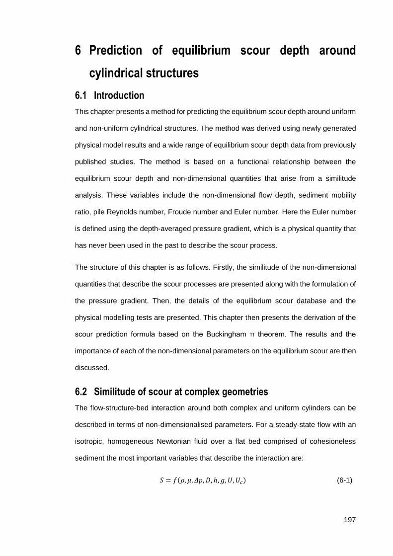
197

6 Prediction of equilibrium scour depth around

cylindrical structures

6.1 Introduction

This chapter presents a method for predicting the equilibrium scour depth around uniform

and non-uniform cylindrical structures. The method was derived using newly generated

physical model results and a wide range of equilibrium scour depth data from previously

published studies. The method is based on a functional relationship between the

equilibrium scour depth and non-dimensional quantities that arise from a similitude

analysis. These variables include the non-dimensional flow depth, sediment mobility

ratio, pile Reynolds number, Froude number and Euler number. Here the Euler number

is defined using the depth-averaged pressure gradient, which is a physical quantity that

has never been used in the past to describe the scour process.

The structure of this chapter is as follows. Firstly, the similitude of the non-dimensional

quantities that describe the scour processes are presented along with the formulation of

the pressure gradient. Then, the details of the equilibrium scour database and the

physical modelling tests are presented. This chapter then presents the derivation of the

scour prediction formula based on the Buckingham π theorem. The results and the

importance of each of the non-dimensional parameters on the equilibrium scour are then

discussed.

6.2 Similitude of scour at complex geometries

The flow-structure-bed interaction around both complex and uniform cylinders can be

described in terms of non-dimensionalised parameters. For a steady-state flow with an

isotropic, homogeneous Newtonian fluid over a flat bed comprised of cohesioneless

sediment the most important variables that describe the interaction are:

𝑆 = 𝑓(𝜌, 𝜇, 𝛥𝑝, 𝐷, ℎ, 𝑔, 𝑈, 𝑈𝑐) (6-1)

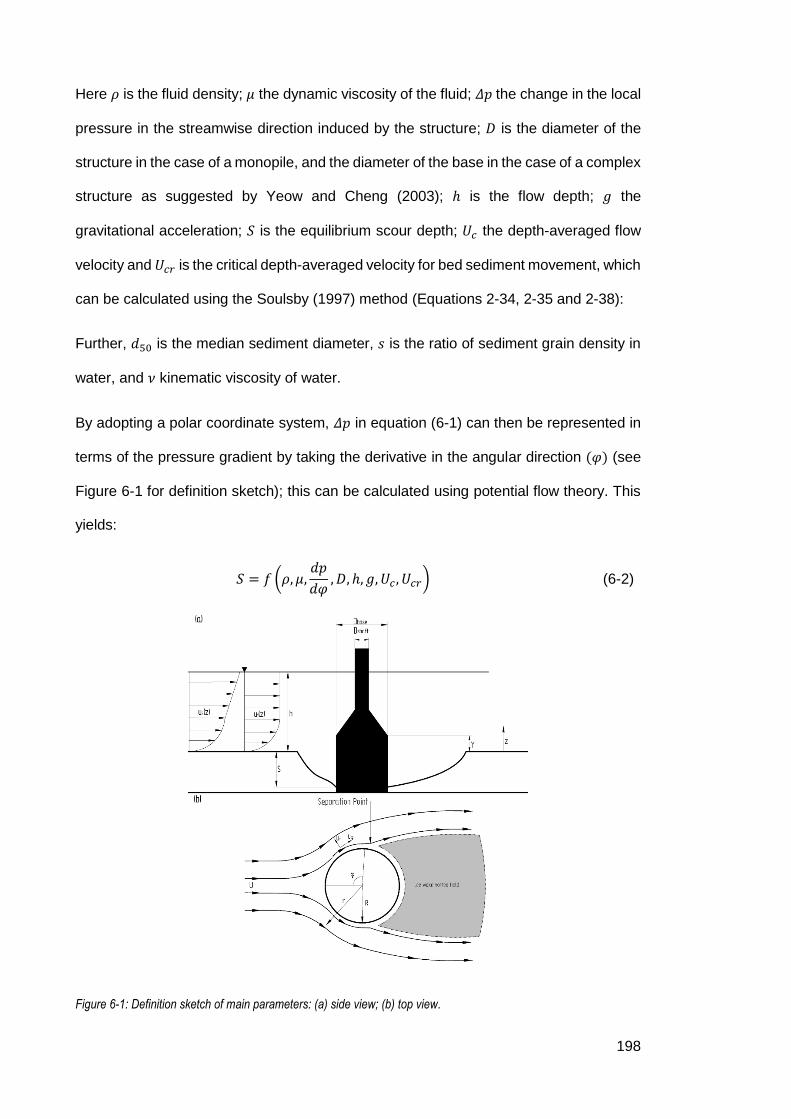
198

Here 𝜌 is the fluid density; 𝜇 the dynamic viscosity of the fluid; 𝛥𝑝 the change in the local

pressure in the streamwise direction induced by the structure; 𝐷 is the diameter of the

structure in the case of a monopile, and the diameter of the base in the case of a complex

structure as suggested by Yeow and Cheng (2003); ℎ is the flow depth; 𝑔 the

gravitational acceleration; 𝑆 is the equilibrium scour depth; 𝑈𝑐 the depth-averaged flow

velocity and 𝑈𝑐𝑟 is the critical depth-averaged velocity for bed sediment movement, which

can be calculated using the Soulsby (1997) method (Equations 2-34, 2-35 and 2-38):

Further, 𝑑50 is the median sediment diameter, 𝑠 is the ratio of sediment grain density in

water, and 𝜈 kinematic viscosity of water.

By adopting a polar coordinate system, 𝛥𝑝 in equation (6-1) can then be represented in

terms of the pressure gradient by taking the derivative in the angular direction (𝜑) (see

Figure 6-1 for definition sketch); this can be calculated using potential flow theory. This

yields:

𝑆 = 𝑓 (𝜌, 𝜇,𝑑𝑝

𝑑𝜑,𝐷, ℎ, 𝑔, 𝑈𝑐 , 𝑈𝑐𝑟) (6-2)

Figure 6-1: Definition sketch of main parameters: (a) side view; (b) top view.

199

By applying the Buckingham π theorem with normalising variables 𝜌, 𝐷 and 𝑈 the

following dependence is obtained for the non-dimensional scour depth 𝑆/𝐷:

𝑆

𝐷= 𝑓(

𝑑𝑝𝑑𝜑

𝑈𝑐2𝜌,Uc

√𝑔ℎ,𝑈𝑐𝑈𝑐𝑟

,𝑈𝐷𝜌

𝜇,ℎ

𝐷) (6-3)

This expression is equivalent to:

𝑆

𝐷= 𝑓 (𝐸𝑢, 𝐹𝑟,


, 𝑅𝑒𝐷,ℎ

𝐷) (6-4)

This expression suggests that the pile Reynolds number (𝑅𝑒𝐷 = 𝑈𝐷/𝜈) is the form of 𝑅𝑒

that best characterises the effect on the scour process. Indeed this is verified when

considering that the flow conditions in most experimental and prototype conditions are

fully developed, thus making viscous effects negligible for a channel 𝑅𝑒 = (𝑈𝑐 ℎ)/𝜈 >

104 (Hughes, 1993). In addition, the critical grain Reynolds number is also considered

implicitly in Equation (6-4) as 𝑈𝑐𝑟 ∝ √𝜃𝑐𝑟 ∝ 𝑅𝑒∗ which implies that the effects of

hydrodynamically rough and smooth flows are also considered through the Shields

parameter 𝜃𝑐.

Both 𝑅𝑒𝐷 and 𝐸𝑢 are of importance in the scour process. The pile Reynolds number

controls two important aspects of the flow structure interaction. Firstly, the separation

point of the flow along the perimeter of a cylinder shifts towards the lee of the pile for an

increasing 𝑅𝑒𝐷 (Achenbach, 1968). This results in a narrower wake, which translates into

a delay in the separation of the boundary layer, a weaker horseshoe vortex at the

upstream face of the structure (Roulund et al., 2005) and a smaller equilibrium non-

dimensional scour depth. Secondly, the frequency of the lee wake vortices is altered. For

cylinders in the same approach flow, the vortex shedding frequency process will be

influenced by any change in the structures’ diameter (i.e. change in the pile Reynolds

number) (Sarpkaya, 2010). This change in 𝑅𝑒𝐷 will result in changes in the size of the

200

vortices and their frequency (Melville, 2008). The importance of turbulent structures at

the lee of structures with respect to scour was confirmed through a series of experiments

by Ettema et al. (2006). In the study the vorticity and shedding frequency around

cylinders were measured, showing that the small cylinders produce twice as much

vorticity compared to the larger cylinders. According to Ettema et al., (2006) this

difference is one of the mechanisms that contribute towards the general tendency of

finding smaller non-dimensional scour depths in prototype conditions compared to

laboratory experiments. This can partially explain the discrepancies between small scale

laboratory experiments and prototype scour measurements, the latter tending to have

relatively small non-dimensional scour depths (Ettema et al., 2006) whereas prototype

observations of scour in the field with live-bed conditions can be large (i.e. scour depth

around 1.8D; Harris and Whitehouse, 2015).

Expression (6-4) shows that both the pile Reynolds number and the Euler number are of

particular importance when attempting to describe the processes involved in scour

around uniform and complex structures. To the author’s knowledge this form of the Euler

number has not previously been used to describe the scour process. In the context of

scour 𝐸𝑢 has only been discussed in Ettema et al. (2006) who argue that, for uniform

cylinders, 𝑈𝑐2/𝑔𝐷 is a form of the Euler number as it emerges from the Euler equation

when applied to a water surface across an eddy. This is equivalent to describing the lee

wake vorticity intensity. The formulation shown in (6-4) differs from most existing scour

prediction formulae (e.g. Khalfin, 1983, for shallow foundations; Breusers et al., 1977;

and Johnson, 1992, for deep foundations) that are based only on:

𝑆

𝐷= 𝑓 (𝐹𝑟,


,ℎ

𝐷) 6-5

As mentioned previously the Euler number is the non-dimensional form of the adverse

pressure gradient induced by the flow-structure interaction. This pressure gradient is

responsible for the formation of the horseshoe vortex and explains the flow structure

201

interaction outside the pile wall boundary layer and outside the lee wake region where

the viscous effects are negligible. By approximating that the flow boundary layer of the

structure is fully developed the pressure at the face of the structure can be determined

by applying Prandtl’s boundary layer theory with the familiar Bernoulli equation in polar

coordinates:

𝑢𝜑2 + 𝑢𝑟

2

2𝑔+𝑝

𝛾+ 𝑧 = 𝐶 (6-6)

where:

𝛾 is the specific gravity of water, p is the pressure, 𝑢𝜑 is the tangential component of the

velocity in polar coordinates with its origin at the centre of the structure, 𝑢𝑟 is the radial

component of the velocity in polar coordinates with its origin at the centre of the structure,

z is the height above the initial bed, and 𝐶 is a constant.

When combined with the equations for the velocity in the tangential and radial direction

this yields equation (6-7):

𝑧 +𝑝

𝛾+1

2𝑔𝑢(𝑧)2(

(𝐷2)

4

𝑟4−2(𝐷2)

2

𝑟2cos(2𝜑) + 1) = 𝐶 (6-7)

And by differentiating with respect to 𝜑:

𝑑𝑝

𝑑𝜑= −2𝜌𝑢(𝑧)2

(

(𝐷(𝑧)2 )

2

𝑟2

)

sin(2𝜑) (6-8)

where:

𝑧 is the vertical distance from the bed, 𝜌 is the density of water, 𝜑 is the angle relative to

the approach flow direction, 𝐷(𝑧) is the diameter of the structure as a function of the

vertical distance from the bed for complex geometries, 𝑑𝑝/𝑑𝜑 is the pressure gradient

at any given location around the structure, 𝑟 is the distance from the pier centre where

202

the pressure gradient is evaluated, and 𝑢(𝑧) is the approach velocity at any given height

“z” above the initial bed.

An estimate of the effect the pressure gradient has on the bed can then be determined

by calculating the depth-averaged pressure gradient (⟨𝑑𝑝/𝑑𝜑⟩) which leads to equation

(6-9).

⟨𝑑𝑝

𝑑𝜑⟩ =

1

ℎ∫

(

−2𝜌𝑢(𝑧)2

(

(𝐷(𝑧)2)2

𝑟2

)

sin(2𝜑)

)

𝑑𝑧ℎ

0

(6-9)

In equation (6-9) the integration assumes that there is no energy transfer between the

fluid layers in the water column and the velocity profile can be approximated by the

equations of the hydrodynamically rough velocity profile given in Einstein (1950) (i.e.

equations (6-10) and (6-11)) and the Nikuradse roughness (Equation (6-12)):

𝑢(𝑧)

𝑈𝑓= 8.6 + 2.5 ln (

𝑧

𝑘𝑠) (6-10)

where:

𝑈𝑓 =𝑈

6.0 + 2.5 ln (ℎ𝑘𝑠)

(6-11)

𝑘𝑠 = 2.5 𝑑50 (6-12)

𝑑50 is the median sediment size; 𝑘𝑠 is the roughness length-scale; ℎ is the water depth

and 𝑈𝑓 is the friction velocity based on the depth-averaged velocity and median sediment

diameter.

203

The maximum depth-averaged pressure gradient can then be determined by integrating

throughout the water column at the point where the maximum tangential pressure

gradient is expected (i.e. 𝜑 = 𝜋/4 𝑎𝑛𝑑 𝑟 = 𝐷𝑏𝑎𝑠𝑒/2) which leads to expression (6-13).

⟨𝑑𝑝

𝑑𝜑⟩𝑚𝑎𝑥 = |

1

ℎ∫ (−2𝜌𝑢(𝑧)2 (

𝐷(𝑧)

𝐷𝑏𝑎𝑠𝑒)

2

)𝑑𝑧ℎ

0

| (6-13)

where 𝐷𝑏𝑎𝑠𝑒 is the diameter of the base of the structure (Figure 6-1a). Equation (6-13)

implies that for the same hydrodynamic conditions the structure that has a non-uniform

structure geometry such as a conical base structure of increasing diameter towards the

bed will have a smaller depth-averaged pressure gradient compared to a monopile. This

in turn would result in a smaller downflow on the face of the structure, a reduced

amplification of the bed shear stress and thus, smaller scour depths. Evidence to support

this statement is provided by Tavouktsoglou et al. (2015) who measured the amplification

of the bed shear stress for the same flow conditions and structures for which the pressure

gradient distribution is calculated in Figure 6-2. The pressure gradients were calculated

for two of the small scale structures listed in Figure 2-2 and for a mean flow velocity of

0.39 m/s and a water depth of 0.165 m. They found that there is a significant increase in

the amplification of the bed shear stress between a conical base structure and a

monopile, which agrees qualitatively with the pressure gradient profiles depicted in

Figure 6-2. Similarly, Equation (6-13) suggests that different vertical distributions of the

incident velocities also have an effect on the pressure gradient and thus on the scour

potential for a given situation. Figure 6-1 (a) shows a structure that has been subjected

to two different flow conditions 𝑢1 and 𝑢2 with different depth profiles but the same overall

flow flux (i.e. same depth-averaged velocity). Applying equation (6-13) to these two

cases, the profile 𝑢2 produces a smaller depth-averaged pressure gradient compared to

that for 𝑢1 as smaller velocities are interacting with the widest portion of the structure.

This phenomenon is of particular interest in practice when considering flows in locations

where large lateral wind loads are expected such as the locations where offshore wind

farms are situated. In these locations the wind load effectively produces a wind driven

204

shear flow on top of the existing logarithmic flow creating a flow profile similar to that of

𝑢2 in Figure 6-1 (a) (Davies and Lawrence, 1994).

Figure 6-2: Pressure gradient distribution through the water column [calculated using Eq. (6-8)] for two different structures under the same flow conditions.

Based on equations (6-3) and (6-13) the non-dimensional form of the depth-averaged

pressure gradient can now be defined as the depth-averaged Euler number, which can

be written as follows:

⟨𝐸𝑢⟩ =⟨𝑑𝑝𝑑𝜑⟩𝑚𝑎𝑥

𝑈𝑐2𝜌

(6-14)

For the simpler case of a logarithmic flow profile interacting with a uniform cylinder the

Euler number can conservatively be assumed to take a value of 2. For all other conditions

designers are recommended to:

establish a functional relationship that describes the vertical distribution of the

streamwise flow velocity (𝑢(𝑧));

create a function that describes the diameter of the non-cylindrical structure

(𝐷(𝑧)) as a function of the distance from the bed (𝑧); and,

calculate the depth-averaged pressure gradient though the integration of

equation (6-13) or by evaluating equation (6-13) at a minimum of 50 points

205

throughout the water column and substituting in expression (6-14). This process

can be automated in a spreadsheet to assist in the calculation of ⟨𝐸𝑢⟩ for different

flow and structural conditions.

Equation (6-14) gives the maximum non-dimensional pressure gradient for a given set

of structural parameters and flow conditions. As stated previously potential flow theory

does not account for the viscous effects within the boundary layer and the lee wake

region; and the vertical integration does not allow for the determination of the vertical

exchange in energy across the face of the structure. For this reason ⟨𝐸𝑢⟩ by itself is not

sufficient to predict the equilibrium scour depth. The remaining parameters in equation

(6-4) are required in order to determine the influence of phenomena and processes not

covered by the Euler number, as will be described later.

6.3 Database Description

A significant amount of equilibrium scour data have been published in the past. In this

study published data on equilibrium scour depths around both uniform and complex

cylindrical structures were selected in order to create an equilibrium scour prediction

equation for clearwater scour conditions. The decision to focus on the clearwater regime

was made in order to avoid data that were influenced by ripple formation upstream of the

structure, which would introduce additional sediment transport scale effects. A summary

of the sources and quantities of scour data is given in Table 6-1 and the distribution of

the most important non-dimensional parameters is given in Figure 6-3.

206

Figure 6-3: Percentage distribution of non-dimensional quantities in database

The data presented include scour tests that were conducted in the clearwater regime for

cohesionless sediments only. Data were included only if all relevant parameters were

presented in the publication. The aforementioned parameters include the median

sediment size, average flow velocity, the sediment geometric standard deviation, water

depth, structural dimensions and the time to equilibrium scour. Tests were discarded if:

they were not run for a sufficiently long period to achieve equilibrium scour.

According to Melville and Chiew (1999) this is the time required to reach a scour

depth in which the scour rate does not exceed 5% of the structure diameter in 24

hours (in scaled time); and,

the sediment geometric standard deviation (𝜎𝑔) was greater than 1.3. This was

done to avoid the effects of bed armouring.

207

Table 6-1: Summary of sources populating the scour database.

Data Source Number of data points

Complex geometries

Amini et al. (2014) 6

Ataie-Ashtiani et al. (2010) 8

Ferraro et al. (2013) 10

Hoffmans and Verheij (1997) 1

Jannaty et al. (2015) 2

Melville and Raudkivi (1996) 7

Moreno et al. (2015) 8

Parola et al. (1996) 13

Present study 40

Simons et al. (2009) 4

Whitehouse et al. (2011a) 2

Total complex geometries 101

Uniform Cylinders

Chabert and Engeldinger (1956) 85

Dey et al. (1995) 18

Ettema (1980) 70

Ettema et al. (2006) 5

Jain and Fischer (1979) 26

Melville (1997) 5

Melville and Chiew (1999) 12

Matutano et al. (2013) 10

Shen et al. (1969) 16

Sheppard and Miller (2006) 4

Sheppard et al. (2004) 4

Yanmaz and Altinbilek (1991) 14

Total uniform cylinders 269

In addition, for a limited number of structures that did not have a circular footprint the

equivalent diameter was determined and used. As a consequence, only one field study

is included in this dataset even though there have been a large number of field studies

published. The majority of field studies were excluded for three reasons:

field measurements tend to have time-varying flows which make it difficult to


in most cases, naturally occurring flows in tidal or alluvial environments are high,

thus forcing scour to occur in the live bed regime for at least part of the time. The

extensive bed formations developed upstream of the structure and the general

208

lowering of the bed would provide additional difficulty in generalising any

information; and,

in most cases it is not possible to monitor the scour development systematically

and, therefore, it is not possible to determine if the scour hole is fully developed.

As Figure 6-3 shows, the majority of the data have a Froude number ranging between 0

and 0.4 which is representative of the 𝐹𝑟 expected in most offshore locations, typically 0

to 0.2. The values of the depth-averaged Euler number are spread over the range of 0

to 1.8, showing that there is a wider distribution of complex geometries, while the

distribution of ⟨𝐸𝑢⟩ is clustered around the value of 2 for the uniform cylinders. This is

explained by the higher pressure gradients expected for uniform cylinders extending to

the water surface. In this dataset the majority of the data points have a mobility ratio

(𝑈𝑐/𝑈𝑐𝑟) value close to 1 for both structure categories yielding the deepest scour for the

given hydrodynamic conditions. In addition, the non-dimensional flow depth is mainly

below 5 for both categories, which is typical of offshore locations where structures are

constructed. Finally, the majority of the data have pile Reynolds numbers smaller than

106, which is due to the lack of prototype data.

6.4 Equilibrium scour depth prediction equation

On non-dimensional grounds the equilibrium scour depth for any structure and flow

condition can be derived through Equation (6-4), assuming that the flow is

incompressible and steady, that the soil consists of cohesionless particles with a low

geometric standard deviation (𝜎𝑔 < 1.3) and the scour is in the clearwater regime. The

main goal of the proposed formula is to provide a tool that is able to predict the

equilibrium scour depth around both complex and uniform structures reliably for

unidirectional currents. This allows for the prediction of scour depths in alluvial

environments accurately and in a conservative manner in offshore conditions as the

action of waves reduces the effects of scour due to tidal action because of its ability to

backfill the scour hole (Sumer et al., 2013).

209

In order to develop the new formula, the general concept presented by Breusers et al.

(1977) is adopted. This describes scour as a function of the product of the governing

non-dimensional parameters (𝑓𝑖) identified as influencing the process. The general form

reads:

𝑆

𝐷𝑏𝑎𝑠𝑒= 𝐹 (∏𝑓𝑖

𝑛

1

) (6-15)

For the development of the present scour prediction equation a first order rational

function was selected as the fitting function which has a general form of:

𝐹(𝑥) =𝑐1𝑥 + 𝑐2𝑥 + 𝑐3

(6-16)

The advantage of this formulation is its sigmoid shape which means that it is constrained

by a pair of horizontal asymptotes. In practical terms this means that the scour depth

described by such a function can never exceed a certain value (𝑆/𝐷𝑏𝑎𝑠𝑒)𝑚𝑎𝑥. On physical

grounds this is reasonable as the equilibrium scour depth around any kind of structure

cannot be infinite. This statement is verified by the statistical analysis of Sumer et al.

(1992) conducted on the tests of Breusers et al. (1977) which yielded that the maximum

non dimensional (within one standard deviation) scour depth around a cylinder is

𝑆/𝐷 =2.

The following paragraphs will present the key steps followed to develop the predictive

equation. The different parameters that influence the equilibrium scour depth have been

presented in equation (6-4) and will be introduced in the parameter study one after the

other in order to investigate the combined influence they have on the scour depth. To

get the best fit the following steps were taken:

a) The general fit function for this study was selected (6-16).

b) Different functional relationships were tried until the highest value of (𝑅2) was

determined.

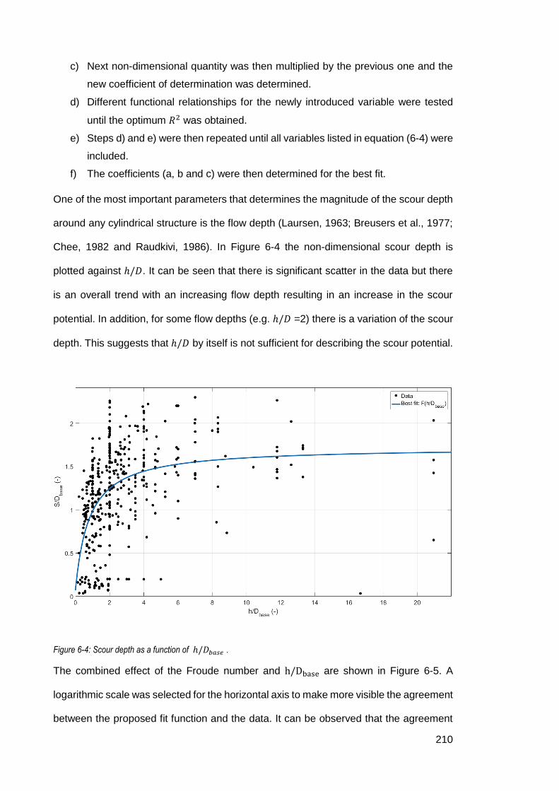
210

c) Next non-dimensional quantity was then multiplied by the previous one and the

new coefficient of determination was determined.

d) Different functional relationships for the newly introduced variable were tested

until the optimum 𝑅2 was obtained.

e) Steps d) and e) were then repeated until all variables listed in equation (6-4) were

included.

f) The coefficients (a, b and c) were then determined for the best fit.

One of the most important parameters that determines the magnitude of the scour depth

around any cylindrical structure is the flow depth (Laursen, 1963; Breusers et al., 1977;

Chee, 1982 and Raudkivi, 1986). In Figure 6-4 the non-dimensional scour depth is

plotted against ℎ/𝐷. It can be seen that there is significant scatter in the data but there

is an overall trend with an increasing flow depth resulting in an increase in the scour

potential. In addition, for some flow depths (e.g. ℎ/𝐷 =2) there is a variation of the scour

depth. This suggests that ℎ/𝐷 by itself is not sufficient for describing the scour potential.

Figure 6-4: Scour depth as a function of ℎ/𝐷𝑏𝑎𝑠𝑒 .

The combined effect of the Froude number and h/Dbase are shown in Figure 6-5. A

logarithmic scale was selected for the horizontal axis to make more visible the agreement

between the proposed fit function and the data. It can be observed that the agreement

211

with the fit function has improved relative to the previous case. Furthermore, below the

yellow line a cluster of data can be observed which corresponds to large scale tests.

In Figure 6-6, the value h/Dbase Fr 1/𝑙𝑜𝑔 (ReD) is plotted against the scour depth. Though

at first glance there is not a big difference with Figure 6-5 the parameter 1/𝑙𝑜𝑔 (ReD) has

helped to reduce the number of outliers which were data corresponding to larger scale

tests and prototype data. More specifically the cluster of data lying below the yellow line

in Figure 6-5 has shifted to the right. This shows the significance of the pile Reynolds

number in describing scaling effects.

The combined influence of ℎ/𝐷𝑏𝑎𝑠𝑒 𝐹𝑟 1/ 𝑙𝑜𝑔(𝑅𝑒𝐷) (𝑈𝑐/𝑈𝑐𝑟)0.5 is shown in Figure 6-7.

The introduction of the factor (𝑈𝑐/𝑈𝑐𝑟)0.5 reduces the scatter of the data. Given that 60%

of the data in this database have 0.85 < 𝑈𝑐/𝑈𝑐𝑟 < 1, the influence of the equation is less

pronounced but the reduction in the outliers is distinct.

Figure 6-5: Scour depth as a function of ℎ/𝐷𝑏𝑎𝑠𝑒 𝐹𝑟 .

Large scale &

prototype data

212

Figure 6-6: Scour depth as a function of ℎ/𝐷𝑏𝑎𝑠𝑒 𝐹𝑟 1/𝑙𝑜𝑔 (𝑅𝑒𝐷) .

Figure 6-7: Scour depth as a function of ℎ/𝐷𝑏𝑎𝑠𝑒 𝐹𝑟 1/ 𝑙𝑜𝑔(𝑅𝑒𝐷) (𝑈𝑐/𝑈𝑐𝑟)0.5 .

After performing the parametric model study, Equation (6-17) which now includes the

Euler number as well was selected as the most effective formula for predicting the non-

dimensional scour depth.

213

𝑆

𝐷𝑏𝑎𝑠𝑒=𝑐1 휁 + 𝑐2휁 + 𝑐3

(6-17)

where:

휁 = (1

log(𝑅𝑒𝐷)) (

ℎ

𝐷𝑏𝑎𝑠𝑒) (𝐹𝑟)(𝐸𝑢)0.5 (


)0.5

(6-18)

𝑐1, 𝑐2 and 𝑐3 are coefficients that were determined through parameter optimisation

according to McCuen and Snyder (1986). Their values for the given data-set with the

corresponding 95% confidence bounds are:

𝑐1 = 2.163 ∈ [2.1, 2.3];

𝑐2 = −0.002 ∈ [−0.009, 0.005]; and,

𝑐3 = 0.03 ∈ [0.01, 0.05].

Figure 6-8 plots the relationship between the non-dimensional scour depth and

parameter 휁. It can be observed that low values of 휁 produce small equilibrium scour

depths while for increasing values of 휁, 𝑆/𝐷𝑏𝑎𝑠𝑒 increases. This behaviour can be

explained by the presence of 𝐷𝑏𝑎𝑠𝑒 at the denominator on the right hand side of Equation

(6-17), which implies that larger structures (in diameter) produce relatively shallower

scour holes while smaller structures create deeper non-dimensional equilibrium scour

depths. This is the behaviour reported by numerous authors such as Ettema et al. (2006).

An example of such large experimental scour depths is in Chiew (1984) who measured

scour depths up to 𝑆/𝐷 = 2.7. This high value is attributed to the effect of the pile

Reynolds number according to Ettema et al. (2006), although a number of examples

have been reported in the literature (e.g. Harris and Whitehouse, 2015) where prototype

scour depths were comparable to those of laboratory experiments (i.e. 𝑆/𝐷~1.8). In

addition to the effect of the pile size several physical phenomena have also been found

214

to contribute to the smaller scour depths in offshore locations. McGovern et al. (2014)

concluded that scour in tidal flows is less than the corresponding scour induced by a

unidirectional current. This conclusion was debated by Harris and Whitehouse (2015)

who showed that scour depths around monopiles in offshore locations subject to tidal

flows fit within the same population as scour induced around piles in unidirectional flows.

This finding is also supported by Porter et al. (2015) who conducted a series of

experiments and found that the scour depth for reversing and unidirectional currents

does not differ. Furthermore, Sumer et al. (2012) concluded, through a series of

experiments, that when the wave climate changes the equilibrium scour depth may be

reduced due to a backfilling process. The previous discussion shows that there are

various phenomena that may partially explain the observation of smaller scour depths at

offshore monopoles in granular soils in some cases, but in general terms scour depths

similar to those induced by unidirectional currents in rivers should be expected. It should

be noted that additional research is required in order to understand the exact

consequences of these phenomena on offshore scour.

Figure 6-8: Scour depth as a function of ζ.

215

During the analysis of the data the velocity profile for a number of tests in the database

were not known and were assumed to be logarithmic and to follow Equation (6-10). This

assumption, along with the fact that laboratory experiments are prone to effects such as

wall friction and non-uniform flow distribution across the width of the flume, are expected

to have contributed to the scatter in Figure 6-8.

The accuracy of the present scour prediction method is evaluated through the

comparison of the predicted scour depths (using equation (6-17)) to the corresponding

measurements. The figure shows that a good agreement is found between the proposed

method and the scour depth database compiled in this study. 55% of the predictions

have an error smaller than 10% and 82% of the predictions an error smaller than 20%.

The values of correlation coefficient (𝑅2) and RMSE (Root Mean Squared Error) were

calculated as 0.91 and 0.16 respectively. It should be kept in mind that a factor

contributing to this high accuracy is that the same database that was used to evaluate

the accuracy of the model was also used to develop it. A limited number of scour

predictors for complex structures are found in the literature. Most of them rely on shape

factors to account for the different structure geometry (e.g. Breusers et al., 1977; Laursen

and Toch, 1956). Scour prediction around GBFs can be calculated through the Khalfin

(1983) method which may lead to the underestimation of the scour depth in some cases.

This is because the method was derived for foundations with a limited skirt depth. Others

provide a conservative method of estimating the equilibrium scour depth through

envelope curves (i.e. FDOT, 2005) which leads to the overestimation of the scour depths

in some cases. Thus the present equation may be a good solution for providing a basis

for the deterministic and probabilistic assessment of scour, which cannot be done with

the other prediction methods.

216

Figure 6-9: Agreement of scour-depth prediction [using Equation (6-17)] and measured scour depths with 10 and 20% confidence bounds

The predictive capacity of the proposed scour prediction equation has been validated

through its comparison with a number of prototype scour measurements around offshore

monopile structures published by ABPmer Ltd et al. (2010). Figure 6-10 shows the

agreement between the present prediction method and the prototype measurements. As

can be seen the present equation is able to predict the scour depth around the structures

with good accuracy even though the scour process in most of these locations is the live

bed scour regime. Exceptions to this observation are the Princess Amalia, Barrow and

Kentish flats locations. In the case of the Princess Amalia site a clay layer at a depth of

2-3m (𝑆/𝐷 ∈ [0.5, 0.75]) was discovered during the geotechnical survey. In general clays

are associated with small scour depths and in many case do not allow any scour. This

explains why the observed scour depths range between 𝑆/𝐷 of 0.5 and 0.8 in Figure

6-10 and why the present predictive equation over-estimates the scour depth at this

location. Barrow is another location situated in an area with a mixture of fine silt and clay

extending to a depth of 10m below the original bed Seacore (2004). This explains the

217

wide range of measured scour depths at this site, as soils mixed with clays may have

variable scour response according to Whitehouse et al., 2011a.

Kentish Flats is located at an area with surficial sediment comprised of muddy sands

(ABPmer Ltd et al., 2010). This also produces variable scour due to the variability in the

mud’s cohesive properties.

Figure 6-10: Comparison of Equation (6-17) with prototype field data.

6.5 Behaviour of scour prediction equation

Having derived the scour prediction formula, the contribution of different physical factors

to its behaviour are assessed.

6.5.1 Influence of depth averaged Euler number

Given that the viscous forces in the flow-structure interaction around piers are negligible,

one needs to find a non-dimensional quantity to describe the flow alteration upstream of

the structure. This implies that a variable that includes the structure length scale and

218

some form of the kinetic energy is required. The depth-averaged pressure gradient in

the form of the Euler number, described earlier in this chapter, includes both of these

physical quantities, and hence it should be possible to describe the two main

mechanisms driving the scour process, which are present upstream of the structure. The

first of these is the horseshoe vortex and the second is the flow acceleration. Potential

flow theory suggests that, given the flow conditions remain constant, an increasing

blockage induced by a structure would result in a larger amplification of the adverse

pressure gradient and thus an increase in the local scour potential. The experiments

conducted in the current study were designed to test this hypothesis and yield results

which relate the depth-averaged Euler number to the equilibrium scour depth for different

structures. Figure 6-11 through 6-13 show the influence that the pressure gradient has

on the equilibrium scour depth for different ranges of sediment mobility parameter, flow

depth and velocity profiles. In these figures the different colours denote a different type

of structure while the different symbols correspond to the different flow conditions. Figure

6-11 shows the influence of ⟨𝐸𝑢⟩ on the equilibrium scour depth for test series 1.0 through

1.28 and the lines correspond to the prediction given by Equation (6-17) for the

corresponding flow conditions. It shows that an increasing Euler number yields an

increase in the equilibrium scour depth given that the remaining flow conditions are the

same and it reaches an asymptotic value of 𝑆/𝐷 as ⟨𝐸𝑢⟩ approaches 2.

Further observation of Figure 6-11 and 6-12 shows that tests conducted with different

sediment sizes but having the same sediment mobility number do not differ significantly

with regards to the equilibrium scour depth. In addition, a decrease in the mobility

parameter (𝑈𝑐/𝑈𝑐𝑟) or (ℎ/𝐷𝑏𝑎𝑠𝑒) results in the same trend described above with respect

to ⟨𝐸𝑢⟩, but with the horizontal asymptote shifting to a lower value of 𝑆/𝐷𝑏𝑎𝑠𝑒.

219

Figure 6-11: Influence of sediment mobility ratio [𝑈𝑐/𝑈𝑐𝑟 =0.74, 0.88 and 1] on the variation of the equilibrium scour

depth as a function of < 𝐸𝑢 > [Note: Line shows prediction given by Equation (6-17) for each of the three sediment mobility ratios.

Figure 6-12: Influence of non-dimensional water depth [ℎ/𝐷𝑏𝑎𝑠𝑒 =3.6 and 2.2] on the variation of the equilibrium

scour depth as a function of < 𝐸𝑢 > [Note: Line shows prediction given by Equation (6-17) for each of the three sediment mobility ratios.

Figure 6-13 shows the results from the larger scale scour tests. It can be observed that

the equilibrium scour depth increases as ⟨𝐸𝑢⟩ increases in the same manner as for the

220

smaller scale tests. Furthermore, the data for complex foundation shapes corresponding

to the non-logarithmic flow profile are shifted further to the left compared to the tests that

were subjected to the logarithmic flow profile, while both test results fall onto the same

trend line. The effect of the non-logarithmic profile on scour for the monopile is less than

for the complex foundation shapes. Given that the depth-averaged flow velocity in both

cases is the same, lower flow velocities are observed near the bed in the case of the

non-logarithmic profile case. This translates to less kinetic energy interacting with the

larger base which yields smaller ⟨𝐸𝑢⟩ and thus smaller scour depths. In addition, given

that all of the remaining non-dimensional flow parameters listed in equation (6-4) are

kept constant during the two tests, it is also expected that both results fall on to the same

curve defined by equation (6-17). Finally, even though the larger scale data plotted in

Figure 6-13 were derived from experiments with slightly different values of the non-

dimensional water depth, mobility ratio and 𝐹𝑟, it can be observed that an increase in the

structural scale of each of the foundation models results in a significant decrease in the

non-dimensional equilibrium scour depth. This effect is linked to the different pile

Reynolds number for this set of tests, and will be elaborated on in the following section.

Figure 6-13: Influence of vertical flow distribution on the variation of the equilibrium scour depth as a function of <𝐸𝑢 > [Note: solid line shows prediction given by Equation (6-17)]

221

6.5.2 Influence of pile Reynolds number

During the large scale experiments two main sediment transport systems were identified:

the sediment from the upstream region of the structure was transported and

deposited at the lee of the structure at an angle 160°-200° relative to the flow

direction. This process is primarily induced by the local increase in the horseshoe

vortex in front of the structure and thus described by the change in 𝐸𝑢, ℎ/𝐷 and

𝐹𝑟; and,

a secondary process that suspends the previously deposited sediment at the lee

of the structure into the water column. This material is then carried away from the

scour hole and deposited further downstream from the structure. This process is

mainly driven by the longitudinal counter-rotating vortices which are created

partly by the horseshoe vortex and the variation of the shedding frequency over

the height of the structure (Baykal et al., 2015; Petersen et al., 2015; Kirkil and

Constantinescu, 2010). Thus this process should be characterised by the pile

Reynolds number.

This finding is presented in Figure 6-14, and shows that the pile Reynolds number is an

important factor controlling the scour process. According to Schlichting (1979) the size

of the pile wall boundary layer is proportional to 1/𝑙𝑛(𝑅𝑒𝐷) which means that the overall

turbulence induced by the flow-structure interaction would decrease as the Reynolds

number increases. In addition Achenbach (1968) showed that an increasing 𝑅𝑒𝐷 forces

the separation point to shift further downstream around the pile, which also results in a

decrease in the sediment transport capacity of the lee wake vortices and thus decrease

the overall scour potential. This shows that 𝑅𝑒𝐷 could account for some scale effects that

result in smaller non-dimensional scour depths for larger scale structures.

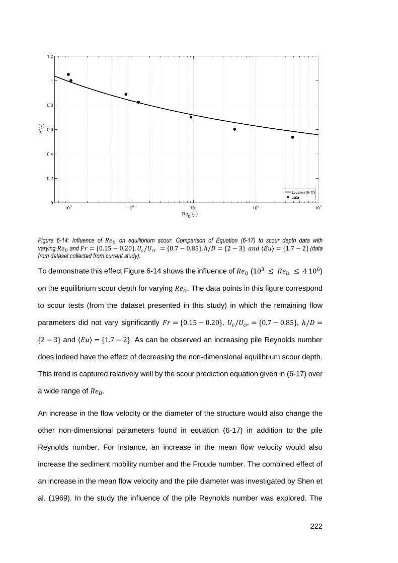
222

Figure 6-14: Influence of 𝑅𝑒𝐷 on equilibrium scour. Comparison of Equation (6-17) to scour depth data with

varying 𝑅𝑒𝐷 and 𝐹𝑟 = {0.15 − 0.20}, 𝑈𝑐/𝑈𝑐𝑟 = {0.7 − 0.85}, ℎ/𝐷 = {2 − 3} 𝑎𝑛𝑑 ⟨𝐸𝑢⟩ = {1.7 − 2} (data from dataset collected from current study).

To demonstrate this effect Figure 6-14 shows the influence of 𝑅𝑒𝐷 (103 ≤ 𝑅𝑒𝐷 ≤ 4 106)

on the equilibrium scour depth for varying 𝑅𝑒𝐷. The data points in this figure correspond

to scour tests (from the dataset presented in this study) in which the remaining flow

parameters did not vary significantly 𝐹𝑟 = {0.15 − 0.20}, 𝑈𝑐/𝑈𝑐𝑟 = {0.7 − 0.85}, ℎ/𝐷 =

{2 − 3} and ⟨𝐸𝑢⟩ = {1.7 − 2}. As can be observed an increasing pile Reynolds number

does indeed have the effect of decreasing the non-dimensional equilibrium scour depth.

This trend is captured relatively well by the scour prediction equation given in (6-17) over

a wide range of 𝑅𝑒𝐷.

An increase in the flow velocity or the diameter of the structure would also change the

other non-dimensional parameters found in equation (6-17) in addition to the pile

Reynolds number. For instance, an increase in the mean flow velocity would also

increase the sediment mobility number and the Froude number. The combined effect of

an increase in the mean flow velocity and the pile diameter was investigated by Shen et

al. (1969). In the study the influence of the pile Reynolds number was explored. The

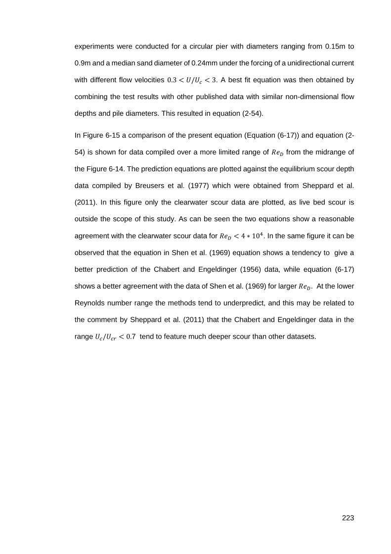
223

experiments were conducted for a circular pier with diameters ranging from 0.15m to

0.9m and a median sand diameter of 0.24mm under the forcing of a unidirectional current

with different flow velocities 0.3 < 𝑈/𝑈𝑐 < 3. A best fit equation was then obtained by

combining the test results with other published data with similar non-dimensional flow

depths and pile diameters. This resulted in equation (2-54).

In Figure 6-15 a comparison of the present equation (Equation (6-17)) and equation (2-

54) is shown for data compiled over a more limited range of 𝑅𝑒𝐷 from the midrange of

the Figure 6-14. The prediction equations are plotted against the equilibrium scour depth

data compiled by Breusers et al. (1977) which were obtained from Sheppard et al.

(2011). In this figure only the clearwater scour data are plotted, as live bed scour is

outside the scope of this study. As can be seen the two equations show a reasonable

agreement with the clearwater scour data for 𝑅𝑒𝐷 < 4 ∗ 104. In the same figure it can be

observed that the equation in Shen et al. (1969) equation shows a tendency to give a

better prediction of the Chabert and Engeldinger (1956) data, while equation (6-17)

shows a better agreement with the data of Shen et al. (1969) for larger 𝑅𝑒𝐷. At the lower

Reynolds number range the methods tend to underpredict, and this may be related to

the comment by Sheppard et al. (2011) that the Chabert and Engeldinger data in the

range 𝑈𝑐/𝑈𝑐𝑟 < 0.7 tend to feature much deeper scour than other datasets.

224

Figure 6-15: Effect of the pile Reynolds number on scour. Comparison of present equation (Equation (6-17)) and the equation of Shen et al, (1969) [Equation 2-54] to the data presented in Breusers et al. (1977) (data source: Sheppard et al., 2011).

6.5.3 Influence of Froude number

According to numerous authors (e.g. Baker, 1986; Graf and Yulistiyanto, 1998) a

significant process that controls the scour process is the strength of the horseshoe

vortex. On physical grounds it can be deduced that the intensity of the horseshoe vortex

should be strongly influenced by the downflow at the face of the structure. Based on the

Bernoulli equation and the conservation of energy it can be concluded that the downflow

is dependent on both the hydrostatic component and the kinetic component of the

energy. Therefore, by applying the Bernoulli equation from a location far away from the

structure (where the flow field is undisturbed) to its leading face, we can obtain:

𝑦

ℎ∝ 𝐹𝑟𝑒 (6-19)

where y is the vertical location of the stagnation point (see Figure 6-16) along the face

of the structure and 𝑒 is a constant.

Figure 6-17 shows the influence of the Froude number on the equilibrium scour depth

for a subset of the data presented in Table 6-1. In this figure the depicted data points

225

have values of the Froude number ranging from 0.11 to 0.97 while 𝑅𝑒𝐷 =

{75000 − 150000},𝑈𝑐/𝑈𝑐𝑟 = {0.8 − 1}, ℎ/𝐷 = {2 − 3} and ⟨𝐸𝑢⟩ = {1.7 − 2}. It can be

observed that the scour depth increases following a logarithmic trend and reaches a

horizontal asymptote as 𝐹𝑟∞. This means that for shallow water depths the high

Froude number results in a stronger kinetic component of the pressure field and,

therefore, in a stagnation point which is closer to the water surface. Thus a larger portion

of the flow is “captured” by the downflow which results in deeper scour depths. On the

other hand, greater flow depths result in smaller Froude numbers which mean that the

hydrodynamic component of the pressure force is larger, effectively creating a more

evenly distributed pressure field along the face of the structure and thus leading to a

vertical stagnation point closer to the bed and, therefore, smaller scour depths (Harris

and Whitehouse, 2015).

Figure 6-16: Definition diagram of the location of the vertical stagnation point.

226

Figure 6-17: Influence of Fr on equilibrium scour. Comparison of Equation (6-17)) to scour depth data with varying 𝐹𝑟

and 𝑅𝑒𝐷 = {75000 − 150000}, 𝑈𝑐/𝑈𝑐𝑟 = {0.8 − 1}, ℎ/𝐷 = {2 − 3} ⟨𝐸𝑢⟩ = {1.7 − 2}.

6.5.4 Influence of non-dimensional flow depth

The flow depth also influences the scour depth in a way that cannot be captured by the

Froude number. According to Sumer and Fredsøe (2002) the boundary layer separation

at the bed will be delayed if the non-dimensional water depth is small, as a smaller ℎ/𝐷

would result in a more uniform flow distribution. This in turn will result in a smaller

horseshoe vortex and, therefore, in a smaller scour potential. Figure 6-18 shows the

influence of the water depth on the non-dimensional scour depth for data where the rest

of the flow conditions do not vary significantly; 𝑅𝑒𝐷 = {100000 − 300000},𝑈𝑐/𝑈𝑐𝑟 =

{0.8 − 1}, 𝐹𝑟 = {0.1 − 0.25} and ⟨𝐸𝑢⟩ = {1.7 − 2}.

227

Figure 6-18: Influence of h/D on equilibrium scour. Comparison of Equation (6-17) to scour depth data with varying h/D

and 𝑅𝑒𝐷 = {100000 − 300000}, 𝑈𝑐/𝑈𝑐𝑟 = {0.8 − 1}, 𝐹𝑟 = {0.1 − 0.25} and ⟨𝐸𝑢⟩ = {1.7 − 2}.

In reality a change in the water depth (ℎ) would affect both the Froude number and the

non-dimensional flow depth (ℎ/𝐷). According to the discussion presented in the previous

sections, an increase in the flow depth would decrease the Froude number and

increase ℎ/𝐷. The combined effect of a change in the water depth while maintaining the

values of the remaining parameters constant is demonstrated in Figure 6-19, where the

clearwater equilibrium scour depth data compiled by Melville and Sutherland (1988) is

also plotted. It can be observed that Equation (6-17) captures the trend of their data well,

albeit with a tendency to over-predict the scour depths for 0.5 < ℎ/𝐷 < 1.5 and under-

predict them for higher values of the non-dimensional flow depth.

228

Figure 6-19: Effect of boundary layer thickness on scour. Comparison of Equation (6-17) with clearwater scour data compiled from Melville and Sutherland (1988).

6.5.5 Influence of the sediment mobility ratio

As mentioned earlier the sediment mobility ratio significantly effects the equilibrium scour

depth potential for a given structure and flow conditions. In the context of the equilibrium

scour Equation (6-17), 𝑈/𝑈𝑐 is a factor that describes the resistance of the local bed to

the hydrodynamic forces that are amplified due to the presence of the structure. The

importance of the sediment mobility ratio on physical grounds can be obtained by

applying the 2D-Vertical continuity equation at a control volume extending from a location

upstream of the scour hole to the deepest point of the scour hole and assuming that at

the equilibrium phase of scour the incoming flow into the scour hole is 𝑈 and the mean

flow velocity at the deepest point of the scour hole is 𝑈𝑐, leading to Equation (6-20):

𝑆

𝐷= 𝑑 (


) 𝑓𝑜𝑟 𝑈 ≤ 𝑈𝑐 (6-20)

229

in which variable 𝑑 is a function of the length of the scour hole in the streamwise direction

at equilibrium and the structure’s diameter.

Figure (6-20) demonstrates the effect of the mobility parameter on the equilibrium scour

for a set of data where 𝑈/𝑈𝑐 varies between 0.35 and 0.99 and 𝑅𝑒𝐷 =

{50000 − 200000}, ℎ/𝐷 = {3 − 6}, 𝐹𝑟 = {0.1 − 0.15} and ⟨𝐸𝑢⟩ = {1.7 − 2}. The data

show reasonably good agreement with Equation (6-17) and with the observations

reported by Melville and Sutherland (1988) who analysed the data of Baker (1986).

Figure 6-20: Effect of sediment mobility ratio on scour for monopiles. Comparison of Equation (6-17) to scour depth

data with varying 𝑈𝑐/𝑈𝑐𝑟𝑎𝑛𝑑 𝑅𝑒𝐷 = {50000 − 200000}, ℎ/𝐷 = {3 − 6}, 𝐹𝑟 = {0.1 − 0.15} 𝑎𝑛𝑑 ⟨𝐸𝑢⟩ ={1.7 − 2}.

230

Part III: Scour protection around complex structures

7 Methodology for scour protection stability tests

7.1 Introduction

An extensive series of tests were conducted to investigate the stability of scour protection

rock (riprap) around the complex structural geometries detailed in section (4.4.1) over a

range of different combinations of waves and currents. A total of 512 tests were

conducted while an additional 16 tests were conducted to investigate the effect long

duration design storm conditions have on the damage development. The main focus of

this study was to establish the amplification of the bed shear stress required to move a

stone of a certain size and density for a given set of flow conditions and structural

geometries.

This chapter describes:

The general scaling and modelling issues concerning the physical modelling of

waves,

The experiment procedures followed for the tests,

The set-up of the experimental facilities used for these tests,

The choice of parameters for the physical models,

The equipment used during the tests; and

The experimental programme for these tests.

7.2 General model and scaling considerations

In addition to the model and scaling considerations presented in section 4.2 the physical

modelling of waves requires the careful consideration of the effect of wave reflection due

to inadequate wave absorption. The present tests were conducted for wave periods

ranging between 1s and 3s which according to Edinburgh Designs Ltd (manufacturers

of wave paddles in this flume) yields negligible reflections (defined as the ratio of the

incoming wave height over the reflected) which are less than 5% (see Figure 7-1).

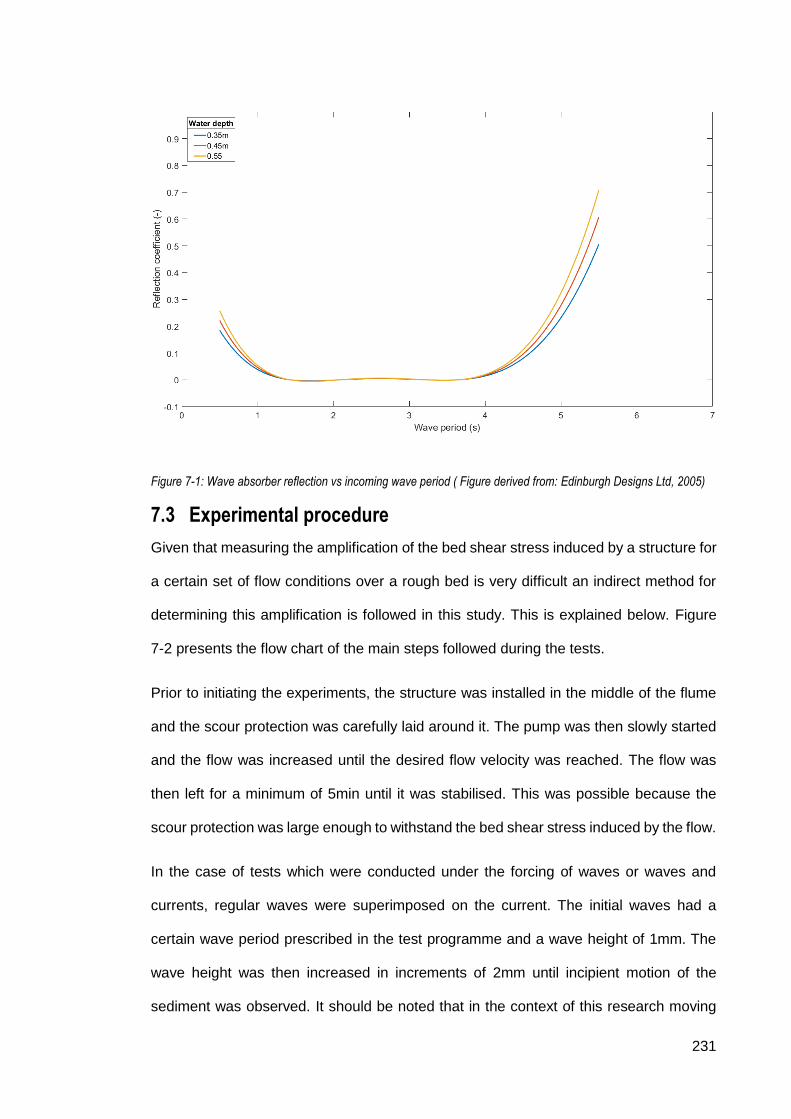
231

Figure 7-1: Wave absorber reflection vs incoming wave period ( Figure derived from: Edinburgh Designs Ltd, 2005)

7.3 Experimental procedure

Given that measuring the amplification of the bed shear stress induced by a structure for

a certain set of flow conditions over a rough bed is very difficult an indirect method for

determining this amplification is followed in this study. This is explained below. Figure

7-2 presents the flow chart of the main steps followed during the tests.

Prior to initiating the experiments, the structure was installed in the middle of the flume

and the scour protection was carefully laid around it. The pump was then slowly started

and the flow was increased until the desired flow velocity was reached. The flow was

then left for a minimum of 5min until it was stabilised. This was possible because the

scour protection was large enough to withstand the bed shear stress induced by the flow.

In the case of tests which were conducted under the forcing of waves or waves and

currents, regular waves were superimposed on the current. The initial waves had a

certain wave period prescribed in the test programme and a wave height of 1mm. The

wave height was then increased in increments of 2mm until incipient motion of the

sediment was observed. It should be noted that in the context of this research moving

232

particles (i.e. undergoing incipient motion) are considered only if the particle is

transported from its original location by more than 2 stone diameters (𝛥𝑥 > 2𝐷50).

In the case of the current only tests the mean current was increased by increments of

~0.05m/s until the rock movement was initiated. After the test was completed the mean

flow velocity profile was measured just upstream of the scour protection.

After the incipient motion was determined for a certain test a new structure was installed

as specified in the experimental programme and the scour protection was repaired.

When a rock at a specific location just starts to move it means that the critical bed shear

stress (𝜏𝑐𝑟𝑖𝑡) at that location has just been reached. This means that the critical bed

shear stress amplification (𝛼𝑐𝑟𝑖𝑡) for that structure can be determined by simply

calculating the undisturbed bed shear stress (𝜏∞) which leads to the incipient motion of

the rock near the structure (i.e. exceedance of critical bed shear stress). This leads to a

modified version of equation (2-39):

𝑎𝑐𝑟𝑖𝑡 =𝜏𝑐𝑟𝑖𝑡𝜏∞

(7-1)

This relation effectively shows by how much the bed shear stress of a certain set of

undisturbed flow conditions gets amplified by the presence of the structure given that the

rocks undergo incipient motion. The numerator in equation (7-1) can be determined using

expressions (2-34) and (2-35), while the undisturbed bed shear stress can be determined

using the following expressions depending on the flow conditions:

Unidirectional current: Equation (2-5)

Waves only: Equation (2-12)

Combined waves and currents (2-26)

Due to the ambiguity in the definition of incipient motion and therefore critical bed shear

stress (i.e. different authors define differently the criterion for which incipient motion is

observed) Yalin’s (1977) incipient motion criterion is adopted (Equation 2-33), which

allows the quantitative definition of this condition.

233

Figure 7-2: Flow chart of experimental procedure.

To investigate which flow conditions lead to the incipient motion of rocks near the

structure, a set of test were conducted to examine the damage pattern induced by these

conditions. This was done by continuing the tests after incipient motion was detected.

The duration of the tests was approximately 10000 waves (both in the case of waves or

waves and currents) or in the case of unidirectional currents 5hr as recommended by the

DNV-OS-H204 manual. In the case where the scour protection at a point was completely

eroded the test was stopped and the scour protection was declared “failed”. Given the

long duration of these tests only a set of representative flow conditions were tested. This

definition of failed scour protection was selected as GBFs cannot accommodate any

scour due to their limited burial depth under the original bed.

7.4 Description of flume and the models

This section will provide an overview of the set-up of the flume and the procedures

followed during the experiments.

The scour protection stability tests were conducted using the same flume and sand pit

configuration as in the large scale scour tests. For a detailed description of the facility

234

and set up of the sand pit the reader is referred to section (4.4.1). Given that the present

tests were conducted under the presence of waves and currents wave probes were

installed upstream and downstream of the structure position (see Figure 7-3)

Figure 7-3: Positions of wave probes (red lines indicate position of the wave probes).

The sand pit was filled with the same fine sand used in the large scale scour tests and

was smoothed flush with the top of the false bed. Two scour protection set-ups were

used in this investigation. In the first case the scour protection was installed above the

original bed level (Figure 7-4 a) while in the second it was installed flush with the original

bed (Figure 7-4 b). It should be noted that the stickup height of the structure relative to

the sand bed remained the same in both configurations. This meant the “true” stickup

height in Figure 7-4 a was reduced by the thickness of the scour protection layer.

Figure 7-4: Layout of scour protection set-up for present tests.

Given that the stability tests were conducted at flow conditions that would mobilize the

fine sediment the entire sand pit was covered with a geotextile with an apparent opening

size of #120 (125μm). This contained the sediment under the cover layer while not

a) b)

235

compromising the hydraulic conductivity of the bed. To ensure that the geotextile was

fully tensioned and did not flap during the experiments it was stapled on the edges of the

sand pit. In addition, U-pins were used to provide extra stability throughout the entire

surface of the geotextile (see Figure 7-5). To prevent sediment from escaping the

puncture holes created by the U-pins, a thin layer of silicon was used to seal potential

gaps. After the geotextile was installed a small hole was opened over the point where

the structure would be installed so it could be screwed into place in a similar way as for

the scour experiments (section 4.3.1.2). The geotextile was then sprayed with an

Nafion™ bonding agent and sprinkled with fine sand to create a roughness similar to that

of the sandy bed. The advantage of the specific binding agent is that it is highly

permeable to water which means the hydraulic conductivity of the sand bed would not

be significantly compromised. To confirm this a constant head test was carried out with

a sample of the geotextile which was laid over a sand sample. The test yielded a

hydraulic conductivity of 4.53 ∗ 10−3cm/s which falls with the range of values expected

for fine sand according to Bear (1972).

Figure 7-5: U-pins used to provide stability to the fabric.

236

Given that the present tests focused on the stability of the top layer of the scour

protection, the scour protection layer extended across the entire width of the flume. This

helped towards avoiding incipient motion of rock located at the side of the scour

protection due to flow contraction between the side wall and the scour protection. The

rock armour extended 5 𝐷𝑏𝑎𝑠𝑒 upstream and downstream of the structure. This length

was selected to minimize the possibility of rock armour being destabilised by the

transition between the original bed level and the scour protection. The leading and trailing

slope of the scour protection had a slope of 30⁰ to provide a smooth transition. Finally,

coloured stones were placed concentrically around the structure to help identify the

movement of rock armour elements. Figure 7-6 presents photographs of the scour

protection layout. The scour protection material was flattened out using a scraper in a

similar way described in section 4.4.1. The concentric circles with the coloured rocks

were placed and flattened by hand.

A number of tests were also conducted with a scour protection set-up identical to that of

Figure 7-4 (a) but without the sand pit. This was done to investigate the effect of

permeability and of the ramp of the sand pit. For these tests a thin baseboard (20mm

thickness) was installed centrally on the bed of the flume, the entire surface of which was

roughened by gluing 0.2mm sand on it. The water depth for these tests was adjusted so

that the water depth was 0.4m from the top of the base board. The structure was then

screwed at its centre and the scour protection was installed around it in the same way

as for the case mentioned above. Given the baseboard’s limited thickness it was not

possible to repeat the tests where the scour protection was flush with the bed using this

apparatus. Figure 7-7 shows a sketch of this set-up.

237

Figure 7-6:Rock armour layer set-up: a) first layer of scour protection b) final layout of scour protection with concentric circles.

Figure 7-7: Test set-up without the sand pit.

a) b)

4𝐷𝑏𝑎𝑠𝑒

Original glass bed of flume

238

Figure 7-8: Large scale foundation geometries

7.5 Flow parameters

The range of hydraulic conditions considered in these tests is shown in Table 7-1.

Regular waves were used because they tend to produce deeper scour than irregular

waves and thus would provide more conservative results. This can be explained by the

varying near bed oscillatory velocities which produce smaller time-averaged bed shear

stresses and thus smaller scour depths (Sutherland and Whitehouse, 1998).

For this test series all current flow velocities were chosen to be in the clear water regime

for the given scour protection material. The critical flow velocity for the sediments used

in the tests was determined in accordance with the Soulsby (1997) method. And, prior to

the scour tests, the critical Shields parameter was determined for a range of different

combinations of waves and currents. This was done by setting a specific flow velocity

and then gradually increasing the wave height until incipient motion was observed. The

corresponding Shields parameter was determined according to the Soulsby method

presented in section (2.2.4). The results of these tests are shown in Figure 7-9. It can be

observed that the Shields diagram agrees well the observations with a maximum

discrepancy of 10%.

239

Table 7-1: Summary of hydraulic conditions for scour protection stability tests

Parameter Units Range

H M 0 – 0.16

T S 1 – 3

H M 0.4

𝑈𝑐 m/s -0.29 – 0.65

𝐷50 Mm 3.5 – 10.5

Figure 7-9: Comparison of Shields parameter with critical bed shear stress for a range of flow velocities.

All structures were tested at a water depth of 400mm (i.e. ℎ/𝐷𝑏𝑎𝑠𝑒=2) which in prototype

conditions corresponds to a water depth of 35-40m. These depths are within the range

in which a number of offshore wind GBFs have been built in the past (e.g. Albatros and

Kårehamn offshore wind parks).

Three different stone sizes were used in the present tests. The mean stone size (𝐷50)

for the aggregates was 3.5mm, 6.5mm and 10.5mm. Given that the purpose of the tests

was to investigate the stability of the stones, the sediments were sieved to obtain the

240

narrowest grading possible. The resulting sediment distribution curves for each of the

three sediments is shown in Figure 7-10. The stones for the scour protection were

angular limestone of medium density. The density (𝜌𝑠) for the 3.5mm and 6.5mm stones

was 2500 kg/m3 and 2550 kg/m3 while the density for the larger 10.5mm aggregate was

2620 kg/m3.

Figure 7-10: Grain size distribution for the scour protection aggregate used in the experiments.

7.6 Measuring techniques

This section provides a description of the measurement techniques used in the present

experiments.

7.6.1 Detection of incipient motion for scour protection

To detect the incipient motion of the sediment two cameras were installed, one on either

side of the flume at an angle of ~45⁰ relative to the bed plane. This made it possible to

monitor the full area surrounding the structure. Both cameras were connected to a PC

and synchronised so that they could start and stop at the same time. After the installation

of the scour protection and the structure the flow was increased with one of two ways:

a) In the case of current only tests: by gradually increasing the undisturbed flow

velocity in increments of approximately ~0.05m/s.

241

b) In the case of combined waves and currents or waves only: for a given set of

wave period and undisturbed flow velocity the wave height was increased until

the rocks started to move.

Figure 7-11: Set-up of incipient motion detection method for scour protection stability tests.

Incipient motion was then determined by subtracting two consecutive frames from the

video recordings. If a rock particle had moved, then the subtraction of the two images

would result in a cluster of pixels with non-zero values. Figure 7-12 presents a pair of

consecutive frames from one of the tests along with the results of the subtraction of the

two. As can be seen the movement of two rocks is clearly captured by this technique. By

identifying the number of non-zero clusters (i.e. moving particles) recorded over a period

of time (t) and area (𝐴𝛺), incipient motion was able to be determined according to Yalin’s

criterion given in Equation (2-33). The advantage of Yalin’s criterion is that it provides a

quantitative criterion for defining incipient motion (ε). This means that for a certain set of

experiments ε should be constant. Based on this rule, if a test was repeated with a larger

rock size of the same specific gravity, then the ratio 𝑚/(𝐴𝛺𝑡) should be decreased in

order to maintain the same ε. Given that for the present tests the area of interest (𝐴𝛺)

was the entire scour protection surface. The values of the time interval (t) and the number

Field of view of camera

242

of displaced particles (m) were then chosen to yield the same value of ε. Table 7-2

provides the chosen values for these tests.

Table 7-2 Values used for determination of incipient motion criterion.

𝐴𝛺 t m 𝐷50 ε

(m2) (s) (-) (mm) (-)

0.502655 10 10 3.5 3.56-05

0.502655 47 10 6.5 3.56-05

0.502655 93 6 10.5 3.57-05

Figure 7-12: Example of particle tracking recognition: a) image at time frame t; b) image at time frame t+1; and c) result of the subtraction of the two images.

7.6.2 Flow velocity measurement

The current velocity flow profile for each flow condition was measured just upstream of

the scour protection before the structure was screwed into place prior to each set of

experiments. For a number of tests, the stability of the scour protection under the forcing

of a unidirectional current was investigated. For these cases the flow velocity was

gradually increased in increments of ~0.05m/s. Once incipient motion of the scour

protection was observed the test was stopped and the full flow profile was measured

10cm upstream of the scour protection edge. All flow measurements were done using

an ADV the working principle of which can be found in section 4.3.3.1

Time frame: t Time frame: t+1

Displaced particles

a) b)

c)

243

7.6.3 Measurement of scour protection damage

Stereophotogrammetry was used to measure the 3D damage pattern around the

structures. The fundamental working principle of Stereophotogrammetry is triangulation.

By taking photographs from a number of different positions lines of sight can be

established between the camera and uniquely identifiable features of the object or

terrain. The process mathematically intersects the lines of sight and produces a three-

dimensional coordinate point cloud of the object. With this technique the position of an

object is determined by different 2D photographs (see Figure 7-13). By taking a sufficient

number of photographs this method can be used to determine the position of both the

camera and the object/target at the same time. The position detection is based on targets

and uniquely identifiable features located on the object (such as different color marks or

rocks) which means that there is no need for a probing system. The advantage of this

method is the high accuracy of the depth measurements which according to Cuypers et

al. (2009) is 10-2cm for a target measuring range smaller than 8×8m. The disadvantage

of this measuring technique is the long computational time required which can take up

to 8hr on a conventional computer.

Figure 7-13: Working principle of photogrammetry [source: Cuypers et al. ,2009]

For these measurements a waterproof Canon PowerShot D20 camera was used.

Photographs were taken from different heights and angles around the structure with a

high overlapping ratio between them (over 80%). This enabled a robust computation of

the coordinates. Given that the camera was hand-held, the experiments had to be

244

paused during the measurement in order to avoid disturbing the local hydrodynamics.

To increase the accuracy of the method two scales were submerged into the flume prior

to taking the photographs to assist in the calibration of the technique. For the analysis of

the photographs Autodesk’s Remake™ software was used.

7.6.4 Wave measurements

The water depth was determined in the same way as for the scour experiments. Rulers

were attached externally on the side wall of the flume and the water depth was

determined by averaging the water depth across all the measuring points to account for

the effect of the hydraulic gradient. Given that the structure was installed in the middle

of the flume the spatially averaged water depth matched the water depth recorded at the

ruler closest to the structure.

The measurement of the wave heights was done using resistance type wave gauges

which were calibrated every day prior to initiating the experiments. The probes were

positioned along the flume at the locations indicated in Figure 7-3 and at a distance 10cm

from the side wall of the flume. The positions from the structure and between them was

selected to comply with the Goda and Suzuki (1976) method for the calculation of the

incident and reflected wave height.

7.7 Experiment programme

Table 7-3 presents the detailed experimental programme for the scour protection stability

tests. The tests are designed to look into the effects of several hydraulic parameters on

the stability of the scour protection material:

Flow direction: the direction of the flow relative to the direction of the wave

propagation was changed in some cases with the waves following (positive sign)

and others opposing (negative sign) the mean flow current.

Wave period: a range of wave periods were tested to investigate the effect of the

wavelength on rock stability.

Rock size: three rock sizes were tested.

Relative current speed: different mean flow velocities (𝑈𝑐𝑤) were tested.

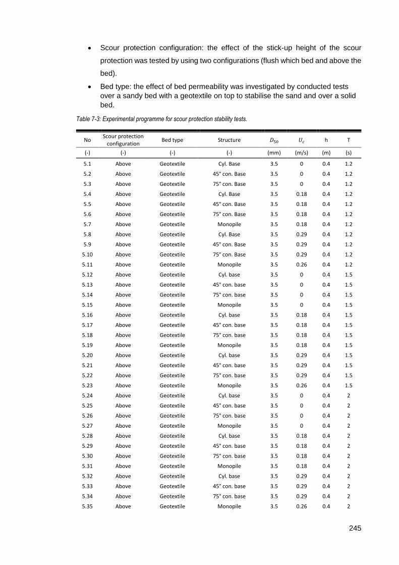
245

Scour protection configuration: the effect of the stick-up height of the scour

protection was tested by using two configurations (flush which bed and above the

bed).

Bed type: the effect of bed permeability was investigated by conducted tests

over a sandy bed with a geotextile on top to stabilise the sand and over a solid

bed.

Table 7-3: Experimental programme for scour protection stability tests.

No Scour protection

configuration Bed type Structure 𝐷50 𝑈𝑐 h T

(-) (-) (-) (-) (mm) (m/s) (m) (s)

5.1 Above Geotextile Cyl. Base 3.5 0 0.4 1.2

5.2 Above Geotextile 45° con. Base 3.5 0 0.4 1.2

5.3 Above Geotextile 75° con. Base 3.5 0 0.4 1.2

5.4 Above Geotextile Cyl. Base 3.5 0.18 0.4 1.2

5.5 Above Geotextile 45° con. Base 3.5 0.18 0.4 1.2


5.7 Above Geotextile Monopile 3.5 0.18 0.4 1.2

5.8 Above Geotextile Cyl. Base 3.5 0.29 0.4 1.2




5.12 Above Geotextile Cyl. base 3.5 0 0.4 1.5

5.13 Above Geotextile 45° con. base 3.5 0 0.4 1.5


5.15 Above Geotextile Monopile 3.5 0 0.4 1.5

5.16 Above Geotextile Cyl. base 3.5 0.18 0.4 1.5

5.17 Above Geotextile 45° con. base 3.5 0.18 0.4 1.5







5.24 Above Geotextile Cyl. base 3.5 0 0.4 2

5.25 Above Geotextile 45° con. base 3.5 0 0.4 2


5.27 Above Geotextile Monopile 3.5 0 0.4 2

5.28 Above Geotextile Cyl. base 3.5 0.18 0.4 2

5.29 Above Geotextile 45° con. base 3.5 0.18 0.4 2


5.31 Above Geotextile Monopile 3.5 0.18 0.4 2





246

5.36 above Geotextile Cyl. base 6.5 0 0.4 1.2

5.37 above Geotextile 45° con. base 6.5 0 0.4 1.2


5.39 above Geotextile Monopile 6.5 0 0.4 1.2

5.40 above Geotextile Cyl. base 6.5 0.18 0.4 1.2

5.41 above Geotextile 45° con. base 6.5 0.18 0.4 1.2


5.43 above Geotextile Monopile 6.5 0.18 0.4 1.2

5.44 above Geotextile Cyl. base 6.5 -0.18 0.4 1.2

5.45 above Geotextile 45° con. base 6.5 -0.18 0.4 1.2


5.47 above Geotextile Monopile 6.5 -0.18 0.4 1.2























5.70 above Geotextile 0 6.5 0 0.4 1.5

5.71 above Geotextile Cyl. base 6.5 0 0.4 2

5.72 above Geotextile 45° con. base 6.5 0 0.4 2

5.73 above Geotextile 75° con. base 6.5 0 0.4 2

5.74 above Geotextile Monopile 6.5 0 0.4 2

5.75 above Geotextile Cyl. base 6.5 0.18 0.4 2

5.76 above Geotextile 45° con. base 6.5 0.18 0.4 2


5.78 above Geotextile Monopile 6.5 0.18 0.4 2

5.79 above Geotextile Cyl. base 6.5 -0.18 0.4 2

5.80 above Geotextile 45° con. base 6.5 -0.18 0.4 2


5.82 above Geotextile Monopile 6.5 -0.18 0.4 2

247





5.87 Above Geotextile Cyl. base 6.5 -0.29 0.4 2

5.88 Above Geotextile 45° con. base 6.5 -0.29 0.4 2


5.90 Above Geotextile Monopile 6.5 -0.29 0.4 2





5.95 Above Geotextile Cyl. base 10.5 0 0.4 1.5



5.98 Above Geotextile Monopile 10.5 0 0.4 1.5





5.103 Above Geotextile Cyl. base 10.5 -0.18 0.4 1.5

5.104 Above Geotextile 45° con. base 10.5 -0.18 0.4 1.5


5.106 Above Geotextile Monopile 10.5 -0.18 0.4 1.5





5.111 Above Geotextile Cyl. base 10.5 -0.29 0.4 1.5



5.114 Above Geotextile Monopile 10.5 -0.29 0.4 1.5

5.115 Above Geotextile Cyl. base 10.5 0 0.4 2



5.118 Above Geotextile Monopile 10.5 0 0.4 2





5.123 Above Geotextile Cyl. base 10.5 -0.18 0.4 2



5.126 Above Geotextile Monopile 10.5 -0.18 0.4 2




248


5.131 above Geotextile Cyl. base 10.5 -0.29 0.4 2























5.154 above Geotextile Cyl. base 10.5 0.65 0.4 0




5.158 flush Geotextile 75° con. base 6.5 0 0.4 1.4



5.161 flush Geotextile 75° con. base 6.5 0 0.4 2





5.166 flush Geotextile 75° con. base 6.5 0 0.4 3

5.167 flush Geotextile 75° con. base 6.5 0.17 0.4 1.4



5.170 flush Geotextile 75° con. base 6.5 0.17 0.4 2







249

5.177 Flush Geotextile 75° con. base 6.5 0.22 0.4 1.6


5.179 Flush Geotextile 75° con. base 6.5 0.22 0.4 2













































250







5.230 flush Geotextile Monopile 6.5 0 0.4 1.4



5.233 flush Geotextile Monopile 6.5 0 0.4 2





5.238 flush Geotextile Monopile 6.5 0 0.4 3

5.239 flush Geotextile Monopile 6.5 0.17 0.4 1.4



5.242 flush Geotextile Monopile 6.5 0.17 0.4 2





























251

5.271 Flush Geotextile Monopile 6.5 0.32 0.4 2.4



5.274 Flush Geotextile Monopile 6.5 0.32 0.4 3




























5.302 Flush Geotextile 45° con. base 6.5 0 0.4 1.4



5.305 Flush Geotextile 45° con. base 6.5 0 0.4 2





5.310 Flush Geotextile 45° con. base 6.5 0 0.4 3








252
















































253











5.375 Flush Geotextile Cyl. base 6.5 0 0.4 1.4



5.378 Flush Geotextile Cyl. base 6.5 0 0.4 2





5.383 Flush Geotextile Cyl. base 6.5 0 0.4 3

5.384 Flush Geotextile Cyl. base 6.5 0.17 0.4 1.4



5.387 Flush Geotextile Cyl. base 6.5 0.17 0.4 2

























254

5.412 flush Geotextile Cyl. base 6.5 0.32 0.4 1.6


5.414 flush Geotextile Cyl. base 6.5 0.32 0.4 2

































5.447 above Impermeable Monopile 10.5 0 0.4 1.5

5.448 above Impermeable Monopile 10.5 0.12 0.4 1.5



5.451 above Impermeable 75° con. base 10.5 0 0.4 1.5

5.452 above Impermeable 75° con. base 10.5 0.12 0.4 1.5







255

5.459 Above Impermeable Cyl. base 10.5 0 0.4 1.5

5.460 Above Impermeable Cyl. base 10.5 0.12 0.4 1.5







5.467 Above Impermeable Cyl. base 3.5 0 0.4 2







5.474 Above Impermeable Cyl. base 3.5 0.06 0.4 2


5.476 Above Impermeable Monopile 3.5 0 0.4 1.2




5.480 Above Impermeable Monopile 3.5 0 0.4 2




5.484 Above Impermeable Monopile 3.5 0.06 0.4 1.4



5.487 Above Impermeable Monopile 3.5 0.06 0.4 2


5.489 Above Impermeable 45° con. base 3.5 0 0.4 1.2




5.493 Above Impermeable 45° con. base 3.5 0 0.4 2




5.497 Above Impermeable 45° con. base 3.5 0.06 0.4 1.4



5.500 Above Impermeable 45° con. base 3.5 0.06 0.4 2






256

5.506 above Impermeable 75° con. base 3.5 0 0.4 2







Table 7-4 shows the programme for the tests which were conducted to examine the

damage pattern induced by flow conditions which just induce incipient motion of the

scour protection material. This was done by continuing the tests after incipient motion

was detected. Given the long duration of these tests only a sample of representative flow

conditions was tested.

Table 7-4: Summary of scour protection damage progression tests.

No Structure D50 U h T

(-) (-) (mm) (m/s) (m) (s)

6.1 Monopile 6.5 0 0.4 1.5

6.2 Monopile 6.5 0.06 0.4 1.5

6.3 Monopile 6.5 0.36 0.4 1.5

6.4 Monopile 6.5 0.39 0.4 0

6.5 75° con. base 6.5 0 0.4 1.5

6.6 75° con. base 6.5 0.06 0.4 1.5

6.7 75° con. base 6.5 0.36 0.4 1.5

6.8 75° con. base 6.5 0.4 0.4 0

6.9 45° con. base 6.5 0 0.4 1.5

6.10 45° con. base 6.5 0.06 0.4 1.5

6.11 45° con. base 6.5 0.36 0.4 1.5

6.12 45° con. base 6.5 0.45 0.4 0

6.13 Cyl. base 6.5 0 0.4 1.5

6.14 Cyl. base 6.5 0.06 0.4 1.5

6.15 Cyl. base 6.5 0.36 0.4 1.5

6.16 Cyl. base 6.5 0.55 0.4 0

257

8 Results for scour protection around complex

structures

This chapter will present the results of the experimental study on scour protection stability

around complex foundation geometries. In this context the flow conditions for all the tests

will be presented, followed by the results for the stability of the scour protection and

results for the development of scour protection damage.

8.1 Flow characteristics

This section presents the measurements of the flow velocity and wave heights for the

present set of experiments.

All flow measurements were undertaken over a flat bed, along the centreline of the flume

and just upstream of the scour protection. The aim was to examine the effect of the scour

protection configuration on the incipient motion. Given the range of different flow

conditions tested in these experiments, the velocity profiles are plotted in a non-

dimensional form for comparison with the Soulsby (1990) method (Figure 8-1). To

distinguish the flow velocities that were opposing the waves with those that were

following the waves the u(z) is non-dimensionalised with the absolute value of the mean

current speed (|𝑈𝑐|). Figure 8-1 shows that there is good agreement between the flow

measurements and Soulsby (1990), though there is a slight tendency for it to under-

predict the velocities near the surface of the flow. In general, it can be assumed that the

present flow conditions resemble these of tidal currents.

258

Figure 8-1: Flow profiles for scour protection stability tests (5.1-5.12 & 6.1-6.16).

Given the large number of wave records acquired during these tests it was not possible

to present all of them in this thesis. For this reason typical water surface profiles for the

waves used in these tests are presented in Figure 8-2. It can be seen that these waves

do not follow the Airy wave theory but rather the 3rd order Stokes theory which is expected

in laboratory tests according to Bosboom and Stive (2012). In addition, Dingemans, 1997

suggests that for Ursell numbers smaller than 32𝜋2/3 ≃ 100 Stokes 3rd order wave

theory is the most appropriate wave theory. Figure 8-3 shows that all of the tests in this

study have 𝑈𝑟 < 100. For this reason, the orbital velocities for these tests are calculated

using the Fenton (1985) explicit solution of the 3rd order Stokes theory.

259

Figure 8-2: Examples of wave profiles from present tests.

Figure 8-3: Distribution of tests as a function of the Ursell number.

260

8.2 Stability of scour protection

8.2.1 Choice of wave friction formula

Given that the present study aims to investigate the critical amplification of the bed shear

stress around complex geometries it is important to select an appropriate method for

calculating the bed shear stress induced by waves. As section 2.2.2 shows there are

many methods for determining the wave friction and thus the bed shear stress.

Figure 8-4 to 8-6 show the non-dimensional bed shear stress (Shields number) as a

function of the sediment size, wave height and wave period given by the different

formulations. It can be observed that all of the methods show similar trends and yield

similar Shields numbers within the range of parameters covered in this study.

When examining the non-dimensional shear stress as a function of the 𝐷∗ (Figure 8-4)

Nielsen (1992), Soulsby (1997) and Swart (1974) yield very similar results. These lie

between the solutions given by Simons et al. (2001) and Myrhaug (1989).

Figure 8-5 shows the effect the wave height has on the bed shear stress based on the

different formulations of the wave friction coefficient along with the range of wave heights

tested during this investigation. It can be seen that again all of the formulations tend to

provide similar solutions with some deviation occurring for small values of the non-

dimensional wave height.

261

Figure 8-4: Effect different wave friction equations have on the wave induced Shields parameter (𝜃) presented as a

function of the non-dimensional stone diameter (𝐷∗) T=1.5s, H=0.16m.


function of the non-dimensional wave height (𝐻/ℎ):T=1.5s, D=6.5mm.

The effect of wave period on the bed shear stress predicted by the five formulations for

wave friction is shown in Figure 8-6. The behaviour of the predictions is similar to that

seen in Figure 8-4. Within the range of wave periods tested in this research the Swart

262

(1974) and Soulsby (1997) approaches yield results which lie in the middle of the

solutions given by Simons et al. (2001) and Myrhaug (1989) which provide an envelope

enclosing the rest of the predictions.

Based on the observations above, the undisturbed bed shear stress due to wave action

will be determined using the Soulsby (1997) method. This is because it tends to provide

an average estimation of the bed shear stress compared to the other methods, not only

within the limits of the present test regime but also outside of it.


function of the non-dimensional wave period (𝑇√𝑔/ℎ): H=0.16, D=6.5mm.

8.3 Analysis of the results of scour protection stability tests

This section presents the results from the scour protection stability tests. The effect of

the individual parameters will first be presented, then the results from all tests will be

combined to derive a design graph that allow designers to select the appropriate stone

size for a scour protection system.

263

8.3.1 Influence of main variables

In the present investigation a range of flow parameters have been tested in order to

obtain a better understanding of the effects different structural and environmental

parameters have on the amplification of the critical bed shear stress and thus the stability

of the scour protection material. The parameter that have been tested in these

experiments are summarized in table 8-1.

Table 8-1: Tested parameters

Variable Units Description

𝑈𝑐 (m/s) Mean flow velocity

H (m) Wave height

L (m) Wavelength

𝐷50 (m) Median stone size

𝛼𝑑𝑖𝑟 (⁰) Flow direction

Scour protection configuration (-) Scour protection flush and above original bed

Permeability of original bed (-) Permeable and impermeable bed

Structural geometry (-) Geometries listed in Figure 7-8

8.3.1.1 Influence of stone size (𝑫𝟓𝟎)

Three different stone sizes were used in the present tests, with median sizes of 3.5mm,

6.5mm and 10.5mm. Figure 8-7 shows a comparison between the critical bed shear

stress amplification induced by the four different geometries as a function of the non-

dimensional stone size (𝐷∗) for three cases: a) waves only with T=2s, b) waves with

T=2s and a mean current 𝑈𝑐=0.18m/s and c) waves with T=2s and a mean current

𝑈𝑐=0.29m/s. The figure shows that there is no influence of the non-dimensional stone

size on the amplification of the bed shear stress for the range of stone sizes tested in

this section. This is because the effect of the roughness and therefore the stone size on

264

the amplification of the bed shear stress is included in 𝛼𝑐𝑟𝑖𝑡 through the critical shear

stress (𝜏𝑐𝑟𝑖𝑡) term in Equation 5-1. In addition, the effect of the geometry of the structure

does not have a significant influence, with all the values of critical bed shear stress

amplification ranging between 1-1.7 and falling within the range of bed shear stress

amplification measured by Sumer et al., 1997 for monopiles.

Figure 8-7: Influence of non-dimensional stone size on the amplification of the bed shear stress for different geometries (lines are linearly interpolated between points): a) waves only; b) 𝑈𝑐 = 0.18𝑚/𝑠 and waves and c) 𝑈𝑐 = 0.29𝑚/𝑠 and waves.

8.3.1.2 Influence of scour protection level

A number of tests were repeated with similar flow conditions over a scour protection

configuration installed flush with the original bed and installed above it (see Figure 7-4).

In all tests the scour protection had the same thickness and the underlying sand bed was

covered with the same geotextile to provide comparable bed conditions. Figure 8-8

presents the results for waves with periods of 1.4s-1.5s and 2s which were imposed onto

currents with a velocity of 0m/s to 0.29m/s. The results show that the scour protection

level does not have a significant effect on the critical amplification and therefore the

stability of the scour protection. This could be expected because when the scour

protection is installed above the original bed the effective area of the structure is reduced

a)

b)

c)

265

(see Figure 7-4) which compensates to a certain level for the increase in the local

velocities due to the local reduction in depth. In addition, the width of the scour protection

is significantly larger than the width recommended by most design guidelines. This

means that the turbulence induced by the transition between the original bed and the

scour protection will have more space to dissipate and therefore the effect it has on the

stability of the scour protection near the structure will be less apparent.

Figure 8-8: Influence of scour protection configuration on the amplification of the bed shear stress for different geometries (lines are linearly interpolated between points): a) waves only, T=1.4-1.5s ; b) waves only, T=2s; c) 𝑈𝑐 =0.18𝑚/𝑠 and waves, T=1.4-1.5s; d) 𝑈𝑐 = 0.18𝑚/𝑠 and waves, T=2s; e) 𝑈𝑐 = 0.29𝑚/𝑠 waves, T=1.4-1.5s; and

f) 𝑈𝑐 = 0.29𝑚/𝑠 waves, T=2s.

8.3.1.3 Influence of bed permeability

The permeability of the bed may have an effect on the hydraulic flow gradients under the

scour protection which may affect stability of the rock cover. Figure 8-9 shows the results

for tests that were conducted under the same hydraulic conditions and scour protection

configuration (scour protection above the bed level). Even though Figure 8-9 shows small

increases and decreases for some cases these deviations remain well within the error

margins associated with this measuring technique. Therefore, as for the other cases

presented in this section the results suggest that the amplification of the bed shear stress

a)

c)

e)

b)

d)

f)

266

is not affected by the bed permeability. This is expected, as the permeability of the rock

cover is O(10) larger than the permeability of the bed and the geotextile. This means that

the hydraulic gradient induced by the water elevation between a wave’s crest and trough

will be insufficient to build-up a large pressure gradient under the rocks.

Figure 8-9: Influence of bed permeability on the amplification of the bed shear stress for different geometries: a) waves

only, T=1.2s and 𝐷50=3.5mm ; b) waves only, T=1.4-1.5s and 𝐷50=3.5mm; c) waves only, T=2s and 𝐷50=3.5mm; d)

waves only, T=1.5s and 𝐷50=10.5mm.

8.3.1.4 Influence of flow direction

Given that the present tests were conducted in a flume, only two flow directions were

tested, with the flow following (positive current velocity) and the flow opposing the waves

(negative current velocity). Figure 8-10 presents the results for a number of tests which

were conducted under the same conditions with flow following and opposing the waves.

The results show that the amplification of the bed shear stress is not significantly affected

by the flow direction. An exception to this is the behaviour of the monopile structure in

the cases c and d. For these flow conditions a current following the waves induces an

amplification which is approximately 30% larger than when the current is opposing the

waves. This can be explained by the fact that the waves in these tests are slightly non-

linear, which means that the orbital velocities under the trough are smaller than the orbital

a)

c)

b)

d)

267

velocities under the crest. This means that the net flow under the crest is going to be

larger when a current is following the waves and thus the amplification of the bed shear

stress larger. The reason why this behaviour is only observed in the case of the monopile

is that this structure has the largest cross-sectional area which means that the

amplification of the local pressure field will be more pronounced than for the other

geometries.

Figure 8-10: Influence of flow direction on the amplification of the bed shear stress for different geometries: a)

𝐷50=6.5mm and T=1.2s ; b) 𝐷50=10.5mm and T=1.5s; c) 𝐷50=10.5mm and T=1.5s; d) 𝐷50=10.5mm and T=2s; and

e) 𝐷50=10.5mm and T=2.5s.

8.3.1.5 Influence of wavelength

For a number of tests, the wave period was varied from 1.2s to 3s to investigate the

effect of the wavelength on the critical bed shear stress amplification. Figure 8-11

presents the influence 𝐷𝑏𝑎𝑠𝑒/𝐿 has on 𝛼𝑐𝑟𝑖𝑡 for the four geometries examined in this

study; in these tests the KC number is smaller than 2. The figure shows that 𝛼𝑐𝑟𝑖𝑡 is fairly

constant for all structures when 𝐷𝑏𝑎𝑠𝑒/𝐿 ≲0.095. After that value the amplification of the

bed shear stress starts to increase and reaches a value of approximately 1.5 which

corresponds to an increase of ~25%. This increase can be explained by the phenomenon

of steady streaming which was explained in section (2.4.3). According to the linear model

a)

c)

e)

b)

d)

268

developed by MacCamy and Fuchs (1954) the phase resolved velocity near the structure

increases as the wavelength decreases (𝐷𝑏𝑎𝑠𝑒/𝐿 increases), which translates into a

larger bed shear stress near the structure. This finding is also supported by the findings

of Sumer and Fredsøe (2001) who conducted scour tests around cylinders in the steady

streaming regime and found that the scour depth increased significantly when 𝐷/𝐿 was

increased from 0.08 to 0.15.

Figure 8-11: Influence of wavelength on the amplification of the bed shear stress for different geometries: 𝐷50=6.5mm , waves only.

8.3.1.6 Influence of the velocity ratio (𝑼𝒄𝒘)

When examining the interaction of combined waves and currents with a structure an

important variable that needs to be considered is the velocity ratio between the mean

current and the bed orbital velocity. Figure 8-12 shows the effect the velocity ratio has

on 𝛼𝑐𝑟𝑖𝑡. In this figure the data correspond to scour protection which has been installed

flush with the original bed with 𝐷50=6.5mm and 1 < 𝐾𝐶 < 5. The results show that the

presence of a superimposed current does not influence significantly the amplification of

the bed shear stress for 𝑈𝑐𝑤 < 0.5 − 0.6. This result may be attributed to the lee wake

269

vortex shedding induced by the current which counteracts the lee wake induced by the

waves.

At higher value of the velocity ratio (i.e. 𝑈𝑐𝑤 > 0.5), the amplification of the bed shear

stress increases significantly for all structures. This can be explained by the current

which in this case is strong enough to establish a constant presence at the lee of the

structure and thus generates more turbulence which in turn results in a larger 𝛼𝑐𝑟𝑖𝑡. The

presence of a strong lee wake vortex is confirmed by the observations during the tests

(see Section 5.5 for a detailed discussion) which revealed that the incipient motion of the

sediment occurred at the lee of the structure. This observation agrees to certain level

with the finding of Sumer and Fredsøe (2001) who found that scour around cylinders

becomes current-dominated when 𝑈𝑐𝑤 ≳ 0.7.

Figure 8-12: Influence of velocity ratio (𝑈𝑐𝑤) on the amplification of the bed shear stress for different geometries:

𝐷50=6.5mm.

8.3.1.7 Influence of the KC number: Design diagram for rock cover size selection

Based on the findings presented in the previous sections two flow parameters have been

identified that have an influence on the amplification of the bed shear stress around

complex geometries. These are the wavelength which has a small effect (Figure 8-11)

270

and the velocity ratio which as seen in Figure 8-12 can result in an increase in 𝛼𝑐𝑟𝑖𝑡 from

O(1) to O(10). This section will present the effect the Keulegan–Carpenter number (KC)

has on 𝛼𝑐𝑟𝑖𝑡. Through its definition KC includes the effect of the wavelength and height

through the bed orbital velocity (𝑈𝑤); thus the effect of the wavelength is also reflected

in KC. Figure 8-13 presents all the experimental results for the four different structures.

In this figure the bottom horizontal axis represents KC, while the top horizontal axis

shows the corresponding amplitude of the wave orbital motion (A). It should be noted,

given that the tests were conducted with structures of the same base diameter (𝐷𝑏𝑎𝑠𝑒),

that KC and A both provide a measure of the amplitude of the wave at the bed. The

colour map shows the value of the velocity ratio. Each line in the figure provides a

conservative estimate of the trend of the data, such that 80% of the data fall below it.

Figure 8-13 shows that there are two distinct trends in the data, as described below.

In the first, a set of data between KC values of 0.5 and 5 has amplification values ranging

between 1 and 2. Closer observation of this subset shows that the velocity ratio is always

smaller than 0.5 which means that they correspond to wave dominated conditions. Thus

the results suggest that the critical amplification of the bed shear stress in a wave

dominated environment is fairly constant with a maximum value of 2.

The second cluster of data shows a large increase in 𝛼𝑐𝑟𝑖𝑡 for values of KC which are

smaller than ~2. The trend for each structure type then splits into four additional sets of

data depending of the structure geometry and reaches its corresponding maximum value

at KC = 0. It should be noted here that a KC of 0 corresponds to the case where no

waves are present which implies that the bed orbital velocity is 0 and thus KC is also 0.

This set of data has velocity ratio (𝑈𝑐𝑤) values ranging between 0.5 and 1 which

corresponds to current dominated flow conditions.

271

Figure 8-13: Influence of the Keulegan–Carpenter number (KC) and the amplitude of the wave orbital motion (A) on the amplification of the bed shear stress for different geometries, the colour map shows the velocity ratio and the lines a conservative estimate of the trend of the corresponding data.

A KC range 1.6-2.1 corresponds to the range values above which the first pair of lee

vortices are created in the case of waves (see Figure 2-19). The formation of these

vortices explains the lift-off of the data for 𝐾𝐶 ≲ 2 which is seen in Figure 8-13:

In the case of wave dominated flows (𝑈𝑐𝑤 < 0.5) the current velocity is weak

relative to the bed orbital velocity (𝑈𝑤).

o When KC≳2 the vortices that are generated by the action of the waves

interact with the lee-wake vortex system generated by the current

structure interaction. Given that the spatial and temporal scales of these

vortices are different their interaction breaks up the turbulent structure of

the lee-wake vortex system. This means that the rock displacement in this

case is mainly attributed to the horseshoe vortex (due to the wave) which

is formed every half-cycle of the wave. This fact is also confirmed by the

findings of Sumer at al., 1992 who found that the maximum lift force

reduces significantly when a current is imposed on an oscillatory flow.

o When KC≲2 no lee vortices are present which mean that the

displacement of the rock is attributed to the steady streaming process.

Both the horseshoe vortex system in waves and the steady streaming are

relatively weak when compared to the horseshoe vortex induced by a current.

272

This explains why 𝛼𝑐𝑟𝑖𝑡 is fairly constant and low throughout the range of KC

values tested in this study.

In the case of current dominated flow (𝑈𝑐𝑤 > 0.5) the current is much stronger

than the bed orbital velocity of the waves.

o This means that when KC≲2 (no lee vortices present) the entire rock

displacement process is driven by the horseshoe vortex and the lee-wake

vortex shedding which are significantly stronger than those generated by

a wave, thus inducing much larger bed shear stress amplification. The

secondary split in the trend lines can be explained by the effect the

structure geometry has on the amplification of the pressure field around

it. structures with a smaller cross-sectional area (thus smaller

amplification in the pressure field) induce smaller values of 𝛼𝑐𝑟𝑖𝑡 than

larger ones (e.g. monopile).

o Since the current intensity is strong, only a small wave (i.e. small KC) is

required to initiate rock movement near the structure. This explains why

there are no data with large values of KC present in the case of current

dominated flows.

Figure 8-13 can also serve as a design diagram for the selection of the appropriate stone

size for the cover layer of a scour protection system and can be used like the Shields

diagram is used for the calculation of the critical Shields number. Figure 8-14 presents a

flow chart outlining the process to be followed to determine the stone size. The first step

in the calculation of the design current and wave condition for a specific site. These can

then be used to calculate the corresponding KC and 𝑈𝑐𝑤 using equations (2-41) and (2-

68). The undisturbed bed shear stress induced by the current (𝜏0) can be calculated

using Equations (2-5) through (2-8) and the corresponding bed shear stress due to

waves (𝜏𝑤) using Equations (2-12) through (2-19). The combined maximum wave and

current bed shear stress (𝜏𝑚𝑎𝑥) can then be determined using the Soulsby (1997)

formulation (Equation 2-26). Having the undisturbed bed shear stress due to the

combined action of waves and currents the next step is to select an stone diameter (𝐷50)

and calculate the corresponding critical bed shear stress using expressions (2-34), (2-

35) and (2-2) which then allows the determination of the quantity 𝛼𝑐𝑟𝑖𝑡 using Equation (7-

273

1). This process provides a pair of values (KC, 𝛼𝑐𝑟𝑖𝑡) which identify a point on Figure

8-13. If that point is below the corresponding design curve, then the selected stone

diameter is too small to resist the local amplified bed shear stress. This means that the

designer needs to re-iterate and select a larger stone size and repeat the process until

the point falls on or above the design curve. There are two types of design curve that

can be selected:

a) Wave dominated curve (red line) which should be selected if the flow conditions

are wave dominated (i.e. 𝑈𝑐𝑤 < 0.5). This curve applies to all structure

geometries.

b) Current dominated curves (black lines) which should be selected in the case of

KC<2.1 and 𝑈𝑐𝑤 > 0.5. In this case the designer should select the curve

corresponding to the structure geometry considered in their design.

Figure 8-14: Flow chart for the calculation of the required stone size for scour protections cover layer.

274

8.3.2 Validation of present results

To validate the outcomes of these experiments the design curves presented in the

previous section have been compared to the experimental results presented in De Vos

(2008), Hjorth (1975), Sumer et al. (1994) and Baykal et al. (2016) who also determined

the maximum amplification of the bed shear stress around structures. The result of the

comparison is shown in Figure 8-15. The largest data set available are the results of De

Vos (2008) who conducted a series of tests to develop an equation capable of calculating

the required stone size for a statically stable scour protection (i.e. incipient motion of

stone cover). These data show good agreement with the design curves, though there is

a slight tendency for the present method to overestimate the critical amplification of the

bed shear stress, especially in the case of current dominated flow conditions. This is

because in the study of De Vos (2008) scour protection cover was classified as “failed”

if one stone had been displaced, while in the present research the Yalin criterion has

been applied which suggests that the critical bed shear stress is reached only if 𝑚

particles are displaced over a certain area and time. This naturally results in an

estimation 𝛼𝑐𝑟𝑖𝑡 which is higher than if only one stone is required to be displaced. An

interesting finding is that the data of De Vos (2008) also suggest that in the case of low

KC numbers (lower than 2) there are two trends, one with high amplification (𝛼𝑐𝑟𝑖𝑡) for

current dominated flows and another with low amplifications for wave dominated flow

conditions.

Figure 8-15 presents equivalent results from Hjorth (1975), Sumer et al. (1994) and

Baykal et al. (2016) who measured (and modelled in the case of Baykal et al., 2016) the

bed shear stress amplification over a smooth bed. These results are not directly

comparable with the results of the present study because the tests were conducted over

a smooth bed which means by definition that 𝜏𝑐𝑟𝑖𝑡 does not exist so nor does 𝛼𝑐𝑟𝑖𝑡.

Theoretically, this means that the amplification of the bed shear stress (𝛼) could take

any value depending on the incoming flow conditions. For this reason, a second vertical

axis representing the values of 𝛼 is introduced on the right hand side of the figure.

275

Though the results of these tests tend to be significantly higher than the ones predicted

by the design curve it can be seen that on a qualitative level the data obtained over a

smooth bed follow the same trend with the wave dominated tests yielding 𝛼 between 1.2

and 4 and in the case of current dominated conditions amplifications up to 11. One more

explanation why these results yield such a high amplification is the small levels of

momentum exchange between the layers of the fluid which translates into larger forces

near the bed in the case of a smooth bed. In the case of a rough bed the shear stress

will be smaller due to the exchange of momentum between the fluid’s layers which

means that more energy is diffused for the same flow conditions thus resulting in smaller

bed shear stresses than in the case of a smooth bed.

Figure 8-15: Comparison of present design curves with published experimental results.

8.4 Development of scour protection damage

This section will present the results for the experiments which investigated the damage

pattern induced by flow conditions which induce incipient motion of the rock cover. The

study involves the measurement of the scour protection damage profile after 500, 1000,

5000 and 10000 waves or the failed profile if it occurred prior to 10000 waves. The results

276

will be presented for each structure geometry separately and a discussion of the results

will be presented at the end of the section.

8.4.1 Monopile damage pattern

Figure 8-16 present the damage pattern induced around the monopile under the forcing

of three different flow regimes, waves only (Test 6.1), waves dominated (Test 6.2) and

current dominated (Test 6.3). The figures show that after the first 1000 waves there is no

significant damage pattern observed though there is some initial erosion which is less

than 1 stone cover diameter (𝐷50). After 5000 waves the clear damage patterns emerge

that have distinct characteristics which depend on the flow regime:

Waves only: The damage occurs at an angle of 45⁰-90⁰ relative to the flow

direction with small deposition areas observed in front and behind the structure.

These locations of deposition are explained by the orbital motion of the waves

near the bed which effectively erode sediment from the sides of the piles (where

the amplification of the pressure is the highest) and deposit it at upstream and

downstream side of the structure where the amplification is lower.

Wave dominated: Here the erosion pattern occurs at the same location as for the

wave only case but most of the deposition occurs as the lee of the structure. This

is due to the current which effectively creates a net sediment transport in the

direction of the mean flow.

Current dominated: Here the presence of a strong current imposed on a small

wave forces most of the damage to occur at the lee of the structure. This can be

attributed to the vortex shedding induced by the stronger current.

It is also observed that though the scour protection in the first two cases has not failed

after N=5000 the cover layer in the case of a current dominated condition failed after

3200 waves. This increased damage rate can also be explained by the higher turbulence

levels associated with the lee-wake vortex shedding.

Figure 8-16 shows that the rock cover for the waves only test failed after 6100 waves

and at N≃7800 in the case of a wave-dominated flow. The rate of damage in the case of

a wave-dominated flow being slower than the wave only case can be explained by the

skewness of the flow which may only be able to remove sediment during one half-cycle

277

of the wave. The location of the failure is consistent with the damage pattern observed

in the previous paragraph.

Figure 8-17 present the damage pattern in the case of a current-only flow. As for the

case of the current-dominated flow conditions presented in Figure 8-16 the majority of

the damage occurs at the lee of the structure. In this case the two distinct scour holes

are wider apart compared to the current-dominated case and can be explained by the

vortex shedding induced by the current-structure interaction. In addition, it can be

observed that the scour protection failed within the same time as the current dominated-

case, the present tests failing after 75min and the current-dominated after 80min. This

suggests that the damage pattern in these two case is mainly attributed to the lee wake

vortex shedding.

278

Waves-only Wave-dominated Current-dominated

Figure 8-16: Damage induced by a cylinder in the following flow regimes: waves only; wave dominated; and current dominated after N number of waves (flow and waves in positive X-direction).

279

Figure 8-17: Damage induced by a cylinder in current only flow conditions after t=1hr and 15min (flow in positive X-direction).

8.4.2 75⁰ conical base

Figure 8-18 show the damage pattern for the 75⁰ conical base for the same flow

conditions as for the monopile case presented in the previous section. The results show

a damage pattern with the same quantitative characteristics for the three flow conditions

considered. It can be observed that there is no deposition in the wave only test. During

the tests it was observed that the majority of the sediment transport occurred in the Y

direction and thus the deposition patterns were not picked up by the photogrammetry

measurements. In the case of the current-dominated tests (i.e. waves & strong current)

the damage pattern is located further downstream of the structure. This may be a result

of the flow being deflected by the slopes of the structure which transports the lee wake

vortices further downstream than in the case of the monopile.

280


Figure 8-18: Damage induced by a 75⁰ conical base structure in the following flow regimes: waves only; wave

dominated; and current dominated after N number of waves (flow and waves in positive X-direction).

281

The damage profile for the 75⁰ conical base structure under the forcing of a unidirectional

current is presented in Figure 8-19. It can be observed that the damage pattern in this

case is similar to that of the monopile in Figure 8-17. The difference here is that the scour

holes are further to the lee of the structure which is consistent with the findings of the

current dominated case. The time to failure for this test was 3hr and 1min which matches

the corresponding time for the current dominated case presented in Figure 8-18 and is

close to N=7589 (i.e. 3hr and 10 min).

Figure 8-19: Damage induced by a 75⁰ conical base structure in current only flow conditions after t=3hr and 1min (flow

in positive X-direction).

282

8.4.3 45⁰ conical base

The damage pattern for the 45⁰ conical base structure is presented in Figure 8-20. As for

the two previously presented geometries the combinations of currents and waves have

the same effect on damage pattern. In the waves-only case no deposition pattern is

observed which was also observed in the wave dominated case of Figure 8-18. During

this test the sediment was transported laterally (Y-direction) and deposited outside the

photogrammetry field of view. This lateral sediment transport may be attributed to the

interaction of the cone with the local hydrodynamics but further investigations need to be

conducted to understand this process.

Figure 8-21 presents the damage pattern induced by a unidirectional current on a 45⁰

conical base structure. It can be seen that the location of the damage coincides with that

observed in the previous cases. In this case the footprint of the damage is smaller than

the two other geometries. This is explained by the smaller shaft diameter which is

interacting with the current which results in lee-wake vortices with a significantly smaller

size. In addition, the location of the damage pattern in the case of the current alone

(Figure 8-21) and current dominated (Figure 8-20) cases is closer to the structure

compared to the 75⁰ conical base structure which can be explained in a similar manner.

283


Figure 8-20 Damage induced by a 45⁰ conical base structure in the following flow regimes: waves only; wave dominated; and current dominated after N number of waves (flow and waves in positive X-direction).

284

Figure 8-21: Damage induced by a 45⁰ conical base structure in current only flow conditions after 3hr and 21min (flow

in positive Y-direction).

8.4.4 Cylindrical base structure

Figure 8-22 presents the damage pattern for the cylindrical base structure under the

forcing of waves only and waves and a small current.

Due to poor image capturing for the remaining two flow conditions no results were able

to be obtained. The damage patterns for the two flow conditions agree with the findings

of the previously presented geometries. In these tests the deposition pattern is altered

slightly with most of the deposition occurring at the lee of the structure in the case of the

waves-only scenario. This finding may be attributed to the non-linearity of the waves (as

discussed in section 8.1) which results in smaller orbital velocities when the flow

reverses. Given that the magnitude of the amplification of the pressure gradient for this

structure is mainly attributed to the cylindrical cap of the structure it can be expected that

under certain wave conditions the wave amplitude during one half-cycle may not be

strong enough to erode sediment and therefore no deposition is required.

285

Waves-only Wave-dominated

Figure 8-22: Damage induced by a cylindrical base structure in the following flow regimes: waves only; and wave dominated after N number of waves (flow in positive Y-direction and waves in Y-direction).

286

8.4.5 Discussion of results

Section 8.3.2 presented the findings of tests that looked into the damage pattern induced

by four types of hydrodynamic conditions on four structural geometries. The results

reveal that geometry does not affect the damage pattern but rather the damage pattern

is influenced by the ambient flow conditions. The results showed that in the case of

waves only and wave dominated conditions the damage occurs at the sides of the

structure. The location of the damage under these flow conditions is attributed to the

steady streaming process and the horseshoe vortex induced by the wave action. In the

case of current only and current dominated flow conditions, the damage occurs at the

lee of the structure due to the increased turbulence induced by the lee-wake vortex

separation. The findings agree well with the findings of De Vos et al., 2008 who also

found that the damage around monopiles occurs at the lee of the structure in the case of

currents and at the sides in the case of waves. Furthermore, the present study showed

that the scour protection will fail (i.e. a portion of the original bed will be uncovered) if

flow conditions that lead to incipient motion of the rock cover persist for a sufficiently long

period of time. This finding agrees with those of Vithana (2013) who found that the initial

displacement of rocks leads to the destabilisation of even more rocks due to the

increased roughness of the bed created by the larger protrusion of the rock. This creates

additional turbulence on the layer of fluid just over the bed armour which enhances the

probability of displacement of a rock element. Finally, it has been observed that the time

to failure of a scour protection system is a function of two factors:

The structure geometry: structures inducing larger depth averaged pressure

gradients induce faster damage rate.

The flow conditions: wave-dominated flow conditions induce a scour rate which

is slower compared to the damage rate induced by a current dominated flow

condition. This difference in the damage rate for different flow conditions is linked

to the different flow structure interaction processes involved in each case.

287

9 Conclusions and recommendations

9.1 Conclusions

The objective of this thesis is to improve understanding of the scour process and scour

protection stability around GBFs. This was achieved through an extensive laboratory test

programme to examine the effects of a range of flow conditions and structural

geometries. To achieve the aims and objectives outlined in chapter 3 a number of novel

measuring techniques were developed and applied. This lead to the development of a

scour prediction equation capable of predicting the equilibrium scour depth around

complex geometries and a design diagram that can be used for the selection of the

appropriate static scour protection rock size.

The first part of this thesis looks into the effect the structure geometry has on the

equilibrium scour depth around such structures. As part of this research a design method

for the prediction of the equilibrium scour depth around uniform and non-uniform

cylindrical structure geometries under clearwater scour conditions is presented. An

equation is derived based on experimental and field data obtained by experiments in this

study and other published work. This method is based on a new physical quantity, the

depth-averaged Euler number, the influence of which is verified through experimental

data collected during this research. The second part of this thesis investigated the

stability of scour protection around the same geometries under the forcing of waves and

currents. The study produced a design diagram that can be used to select the

appropriate stone size for specific undisturbed flow conditions based on the structure

geometry. The method shows good agreement with experimental data of other authors.

In addition to the methods for the calculation of the scour depth and optimum scour

protection size, several conclusions have also been reached through this study:

1. The flow measurements around the structures revealed the existence of a

clockwise recirculating cell at the lee of the cylindrical base structure. This

288

recirculation cell can explain the significant reduction of the scour depth at

the lee of the specific structure.

2. The analysis of the equilibrium scour depth data showed that the equivalent

pile diameter is not an appropriate length scale to normalise the scour depth.

Structures with thin top shafts can lead to equivalent diameters with very low

values which in turn result in values of 𝑆/𝐷𝑒𝑞 which are unrealistically high.

3. The tests showed that the scour pattern around the structures is linked to the

geometry of the structure with the complex structure inducing different scour

patterns from the monopile. In addition, there is no clear evidence that the

upstream scour slope is dependent on the geometry or the incoming flow

conditions. In general, the slopes in all tests ranged between 30⁰ and 45⁰

which correspond to the upper limit of the angle of repose for submerged

sands. The downstream slope varies from 0⁰ to 45⁰ and seems to depend

both on the structure geometry and the hydrodynamics. The results also

revealed that the structural geometry has a significant effect on the scour

development and the equilibrium scour depth. Structures with larger cross-

sectional areas induce more rapid and deeper scour while smaller ones

slower and more shallow scour holes. This behaviour is linked to the effect

the geometry has on the local change in the pressure gradient and on the

surrounding bed. Results from the tests also suggest that changes of the

incoming flow profiles result in changes in the scour depths. This can be

explained with the same line of logic.

4. The flow measurements around the structures show that the monopile has a

different hydrodynamic behaviour compared to the conical base structures,

while the cylindrical base structure has similarities with both of the

aforementioned structures. The measurements showed that the

discontinuities between the different geometrical components of the structure

induce flow separation.

5. The results from the pressure measurements show good agreement with

potential flow theory. In addition, the equilibrium scour depth results show

good agreement with the non-dimensional depth averaged pressure gradient.

Based on these findings it can be concluded that potential flow theory can be

used to calculate the Euler, which is an important physical quantity

characterising the equilibrium scour depth.

6. Other physical quantities influencing the equilibrium scour depth have been

identified as 𝑅𝑒𝐷, 𝐹𝑟, 𝑈𝑐/𝑈𝑐𝑟, and ℎ/𝐷.

289

7. The incipient motion detection method that was developed in this study was

used to determine the critical bed shear stress for different combinations of

wave and currents (Figure 7-9) and was found that the results fall within 10%

of the predictions of 𝜏𝑐𝑟𝑖𝑡 given by the Soulsby (1997) method.

8. Scour protection stability tests showed that the following parameters do not

have a significant influence on the critical amplification of the bed shear stress

(𝛼𝑐𝑟𝑖𝑡) around the geometries tested in this study:

a. Stone size (𝐷50)

b. Bed permeability

c. Flow direction

d. Scour protection configuration

9. It was found that for the waves tested in this study, waves opposing a current

did not significantly affect the amplification of the bed shear stress around the

structures.

10. The stability of the scour protection is mainly a function of the KC and 𝑈𝑐𝑤. It

was found that for wave dominated flow (𝑈𝑐𝑤 < 0.5) the critical amplification

of the bed shear stress is constant and does not exceed the value of 2. For

current dominated flows (𝑈𝑐𝑤 > 0.5) 𝛼𝑐𝑟𝑖𝑡 increases significantly as the KC

value decreases and is dependent on the structure geometry.

11. The location of the damage is not dependent on the structure geometry. It

rather depends on the incoming flow conditions with current dominated flows

inducing damage patterns at the lee of the structure, whereas wave-

dominated flow damage occurs at the sides of the structure.

12. Scour protection that undergoes incipient motion will fail as long as the flow

conditions persist for a sufficiently long period.

290

9.2 Recommendations

The increasing computation power of modern computers and the development of new

Computational Fluid Dynamics (CFD) solvers, means that the field of hydraulic

engineering is increasingly reliant on the results of such programmes and less on the

results of physical modelling. The outcomes of the present research and more

specifically the scour prediction method can be easily coupled with CFD solvers to

determine the scour depth around complex geometries in a computationally efficient

manner. Such solvers require extensive validation campaigns which in turn require

experimental results which are also provided in this research.

In addition, the present research has opened a number of possibilities for further

research which are presented below:

In terms of scour:

o The scour prediction equation applicability could be expanded to include

the effects of live bed scour and more complex geometries (e.g. jacket

foundation, tripods and substations). Additional, experiments are required

to fully evaluate these effects.

o As only two structural scales were tested in this study, more experiments

at a larger scale would complement the results and provide further

insights the associated effects on scour.

o Further research is required to understand the causes of avalanching at

the edge of the scour hole that were observed during experiments 3.5-

3.8.

In terms of the scour protection stability:

o The accuracy of the incipient motion detection method could be further

increased by applying more sophisticated particle tracking algorithms and

using more accurate and advanced measuring devices.

o Additional experimental and numerical studies could provide valuable

insights on the underlying physics which lead to the sudden increase in

the bed shear stress amplification for 𝑈𝑐𝑤 > 0.5.

o During this test the sediment was transported laterally (Y-direction) and

deposited outside the photogrammetry field of view. This lateral sediment

transport may be attributed to the interaction of the cone with the local

291

hydrodynamics but further investigations need to be conducted to

understand this process.

o The application range of the design chart for the selection of the

appropriate stone size for scour protection can be increased by

conducting more experiments at larger 𝐾𝐶 values, varying flow depths,

protection thicknesses and structure sizes. In addition, incorporating the

Euler number as a variable describing the effects of the structures

geometry can also lead to the application of this method to a wider range

of geometries.

o The results provide valuable insights into the scour protection damage

progression. More experimental data on the topic provide valuable insight

and could allow the development a prediction method.

o It should be kept in mind that small scale experiments might be subject to

scale and model effects. Verification of the results with large scale models

and prototype measurements is indispensable.

292

10 References

Achenbach, E. (1968). Distribution of local pressure and skin friction around a

circular cylinder in cross-flow up to Re= 5× 10 6. Journal of Fluid Mechanics, 34(4), 625-

639.

ABPmer Ltd et al. (2010). A Further Review of Sediment Monitoring Data.

Commissioned by COWRIE Ltd (project reference ScourSed-09).

Amini, A., Melville, B. W., Ali, T. M., and Ghazali, A. H. (2011). Clear-water local

scour around pile groups in shallow-water flow. Journal of Hydraulic Engineering, 138(2),

177-185.

Ataie-Ashtiani, B., Baratian-Ghorghi, Z., and Beheshti, A. A. (2010). Experimental

investigation of clear-water local scour of compound piers. Journal of Hydraulic

Engineering, 136(6), 343-351.

Baker, C. J. (1978). Vortex flow around the bases of obstacles (Doctoral

dissertation, University of Cambridge).

Baker, C. J. (1979). The laminar horseshoe vortex. Journal of Fluid Mechanics,

95(02), 347-367.

Baker, C. J. (1980). The turbulent horseshoe vortex. Journal of Wind Engineering

and Industrial Aerodynamics, 6(1), 9-23.

Baker, C. J. (1985). The position of points of maximum and minimum shear stress

upstream of cylinders mounted normal to flat plates. Journal of wind engineering and

industrial aerodynamics, 18(3), 263-274.

Baker, C. J. (1991). The oscillation of horseshoe vortex systems. Journal of Fluids

Engineering, 113(3), 489-495.

293

Baker, R. E. (1986). Local scour at bridge piers in non-uniform sediment. Thesis

presented to the university of Aukland, New Zealand, in partial fulfilment of the

requirements for the degree of Master of Philosophy.

Baykal, C., Sumer, B. M., Fuhrman, D. R., Jacobsen, N. G., and Fredsøe, J.

(2015). Numerical investigation of flow and scour around a vertical circular cylinder.

Philosophical Transactions of the Royal Society of London A: Mathematical, Physical

and Engineering Sciences, 373(2033), 20140104.

Bear, J. (1972). Dynamics of fluids in porous materials. Society of Petroleum

Engineers.

Bijker, E. W., and De Bruyn, C. A. (1989). Erosion around a pile due to current and

breaking waves. In Coastal Engineering 1988 (pp. 1368-1381).

Blanco, M. I. (2009). The economics of wind energy. Renewable and Sustainable

Energy Reviews,813(6), 1372-1382.

Blevins, R. D., and Burton, T. E. (1976). Fluid forces induced by vortex shedding.

Journal of Fluids Engineering, 98(1), 19-24.

Bonasoundas, M. (1973). Non-stationary Hydromorphological Phenomena and

Modelling of Scour Process. In Proc. 16th IAHR Congress (Vol. 2, pp. 9-16).

Bos, K. J., Chen, Z., Verheij, H. J., Onderwater, M., and Visser, M. (2002a). Local

scour and protection of F3 offshore GBS platform. In ASME 2002 21st International

Conference on Offshore Mechanics and Arctic Engineering (pp. 219-230). American

Society of Mechanical Engineers.

Bos, K. J., Verheij, H. J., Kant, G., and Kruisbrink, A. C. H. (2002b). Scour

protection around gravity based structures using small size Rock. In First International

Conference on Scour of Foundations.

294

Bosboom, J., and Stive, M. J. (2012). Coastal Dynamics I: Lectures Notes

CIE4305. VSSD.

Briaud, J. L. (2004). Pier and contraction scour in cohesive soils (Vol. 516).

Transportation Research Board.

Breusers, H. N. C. (1965). Conformity and time scale in two-dimensional local

scour. Waterloopkundig Laboratorium.

Breusers, H. N. C. (1971). Local scour near offshore structures. Publication. Delft

Hydraulics Laboratory Publikatie-Waterloopkundig Laboratorium.

Breusers, H. N. C., and Raudkivi, A. J. (1991). Scouring, hydraulic structures

design manual. IAHR, AA Balkema, Rotterdam, 143.

Breusers, H. N. C., Nicollet, G., and Shen, H. W. (1977). Local scour around

cylindrical piers. Journal of Hydraulic Research, 15(3), 211-252.

Buffington, J.M., and Montgomery, D.R. (1997). A systematic analysis of eight

decades of incipient motion studies, with special reference to gravel-bedded rivers:

Water Resources Research. v. 33, p. 1993-2029.

Cardoso, A. H. and Bettess, R. (1999). Effects of time and channel geometry on

scour at bridge abutments, J. Hydraul. Eng., 125:4, 388-399.

Carroll, B., Cooper, B., Dewey, N., Whitehead, P., Dolphin, T., Rees, J., Judd, A.,

Whitehouse, R. and Harris, J. (2010). A further review of sediment monitoring data.

Cowrie ScourSed-09, Southampton, UK, 106.

Carstens, T. (1976). Seabed scour by currents near platforms. Mar. Sci. Commun.,

2(1), 69-93.

Chabert, J., and Engeldinger, P. (1956). Study of scour around bridge piers. Rep.

Prepared for the Laboratoire National d’Hydraulique

295

Chee, R. K. W. (1982). Live-bed scour at bridge piers. Publication of: Auckland

University, New Zealand, (290).

Chen, H. H., Yang, R. Y., Kuo, P. C., and Hwung, H. H. (2012). Physical modeling

study on scour and scour countermeasure for sea-crossing bridge piers. Coastal

engineering proceedings, 1(33), 83.

Chiew, Y. M. (1984). Local scour at bridge piers (Doctoral dissertation,

ResearchSpace@ Auckland).

Chiew, Y. M. (1995). Mechanics of riprap failure at bridge piers. Journal of

Hydraulic Engineering, 121(9), 635-643.

Chou, J. H., and Chao, S. Y. (2000). Branching of a horseshoe vortex around

surface-mounted rectangular cylinders. Experiments in fluids, 28(5), 394-402.

Christoffersen, J. B., and Jonsson, I. G. (1985). Bed friction and dissipation in a

combined current and wave motion. Ocean Engineering, 12(5), 387-423.

Coleman, S. E. (2005). Clearwater local scour at complex piers. Journal of


Dargahi, B. (1989). The turbulent flow field around a circular cylinder. Experiments

in Fluids, 8(1-2), 1-12.

Davies, A. M., and Lawrence, J. (1994). Examining the influence of wind and wind

wave turbulence on tidal currents, using a three-dimensional hydrodynamic model

including wave–current interaction. Journal of Physical Oceanography, 24(12), 2441-

2460.

De Vos, L., De Rouck, J., Troch, P., and Frigaard, P. (2011). Empirical design of

scour protections around monopile foundations: Part 1: Static approach. Coastal

Engineering, 58(6), 540-553.

296

De Vos, L., De Rouck, J., Troch, P., and Frigaard, P. (2012). Empirical design of

scour protections around monopile foundations. Part 2: Dynamic approach. Coastal

Engineering, 60, 286-298.

Den Boon, J. H., Sutherland, J., Whitehouse, R., Soulsby, R., Stam, C. J. M.,

Verhoeven, K., and Hald, T. (2004). Scour behaviour and scour protection for monopile

foundations of offshore wind turbines. EWEC, London, UK.

Dey, S., Bose, S. K., and Sastry, G. L. (1995). Clear water scour at circular piers:

a model. Journal of Hydraulic Engineering, 121(12), 869-876.

Dey, S., and Raikar, R. V. (2007). Characteristics of horseshoe vortex in

developing scour holes at piers. Journal of Hydraulic Engineering, 133(4), 399-413.

Dietz, J. W. (1972). Ausbildung von Langen Pfeilern bei Schraganstromung am

Beispiel der BAB-Mainbrucke Eddersheim. Mitteilungsblatt der BAW, 31, 79-94.

Dixen, M., Hatipoglu, F., Sumer, B. M., and Fredsøe, J. (2008). Wave boundary

layer over a stone-covered bed. Coastal Engineering, 55(1), 1-20.

Eadie IV, R. W., and Herbich, J. B. (1986). Scour about a single, cylindrical pile

due to combined random waves and a current. In Coastal Engineering 1986 (pp. 1858-

1870).

Ettema, R. (1976). Influence of bed gradation on local scour: New Zealand,

University of Auckland, School of Engineering (No. 124). Report.

Ettema, R. (1980). Scour at bridge piers (No. 216 Monograph).

Ettema, R., Kirkil, G., and Muste, M. (2006). Similitude of large-scale turbulence in

experiments on local scour at cylinders. Journal of Hydraulic Engineering, 132(1), 33-40.

Fael, C. M. S., Simarro‐Grande, G., Martín‐Vide, J. P., and Cardoso, A. H. (2006).

Local scour at vertical‐wall abutments under clear‐water flow conditions. Water

resources research, 42(10).

297

Florida Department of Transportation (FDOT). (2005). Bridge scour manual,

Tallahassee, FL.

Fenton, J. D. (1985). A fifth-order Stokes theory for steady waves. Journal of

waterway, port, coastal, and ocean engineering, 111(2), 216-234.

Ferraro, D., Tafarojnoruz, A., Gaudio, R., and Cardoso, A. H. (2013). “Effects of

pile cap thickness on the maximum scour depth at a complex pier.” J. Hydraul. Eng.,

10.1061/(ASCE)HY.1943-7900.0000704, 482–491.

Fredsøe, J., and Deigaard, R. (1992). Advanced series on ocean engineering.

World Scientific, 3, 392.

Fredsøe, J., and Sumer, B. M. (1997). Scour at the round head of a rubble-mound

breakwater. Coastal engineering, 29(3-4), 231-262.

Friedrichs, C. T., and Aubrey, D. G. (1994). Tidal propagation in strongly

convergent channels. Journal of Geophysical Research: Oceans, 99(C2), 3321-3336.

Froehlich, D. C. (1988). Analysis of onsite measurements of scour at piers. In

Hydraulic Engineering: Proceedings of the 1988 National Conference on Hydraulic

Engineering (pp. 534-539).

Giilqe, T., Sumer, B.M. and Fredsøe, J., (1994). Scour around the head of a

vertical-wall breakwater. In: Proc. International Conf. on Hydro-Technical Engineering

for Port and Harbor Construction, Yokosuka, pp. 1097-1116.

Graf, W. H., and Yulistiyanto, B. (1998). Experiments on flow around a cylinder;

the velocity and vorticity fields. Journal of Hydraulic Research, 36(4), 637-654.

Grune, J., Sparboom, U., Schmidt-Koppenhagen, R., Wang, Z., and Oumeraci, H.

(2006). Stability tests of geotextile sand containers for monopile scour protection. In

Coastal Engineering Conference (Vol. 30, No. 5, p. 5093). ASCE American Society of

Civil Engineers.

298

Guo, J. (2012). Pier scour in clear water for sediment mixtures. Journal of Hydraulic

Research, 50(1), 18-2

Hannah, C. (1980). Scour at pile groups. University of Canterbury Library.7.

Hansen, N. E. O., and Gislason, K. (2005). Movable scour protection on highly

erodible sea bottom. In International Coastal Symposium.

Harris, J.M. and Whitehouse, R.J.S. (2015). Marine scour: Lessons from Nature’s

laboratory. In: Scour and Erosion, Proc. 7th Int. Conf. on Scour and Erosion, The

University of Western Australia, 2 - 4 December, 2014, (eds.) Cheng. L., Draper, S. and

An, H., CRC Press, p. 19 - 31(Keynote).

Herbich, J. B. (1984). Seafloor scour: Design guidelines for ocean-founded

structures (Vol. 4). Marcel Dekker Inc.

Hjorth, P. (1975). Studies on the nature of local scour. Department of Water

Resources Engineering, Lund Institute of Technology, University of Lund, Sweden, Bull

Series A 46.

Hjulstrom, F. (1939). Transportation of detritus by moving water: Part 1.

Transportation.

Holmedal, L. E., and Myrhaug, D. (2013). Combined tidal and wind driven flows

and bedload transport over a flat bottom. Ocean modelling, 68, 37-56.

Hoffmans, G. J. C. M. (1990). Concentration and flow velocity measurements in a

local scour hole. TU Delft, Department of Hydraulic Engineering.

Hoffmans, G. J. (2012). The influence of turbulence on soil erosion (Vol. 10).

Eburon Uitgeverij BV.

Hoffmans, G. J., and Verheij, H. J. (1997). Scour manual (Vol. 96). CRC Press.

Hofland, B. (2005). Rock and roll: Turbulence-induced damage to granular bed

protections. TU Delft, Delft University of Technology.

299

Hughes, S. A. (1993). Physical models and laboratory techniques in coastal

engineering (Vol. 7). World Scientific.

Hughes, S. (2003). Physical modelling considerations for coastal structures. In:

Advances in Coastal Structure Design, Edited by Mohan, R. K., Magoon, O. and Pirrello

M.

Isbash, S. V. (1935). Construction of dams by dumping stones in flowing water.

U.S. Army Engr. District, Eastport, Maine.

Jain, S. C., and Fischer, E. E. (1979). “Scour around circular bridge piers at high

Froude numbers.” No. FHWA-RD-79-104 Final Rep., Federal Highway Administration,

Washington, DC.

Jannaty, M. H., Eghbalzadeh, A., and Hosseini, S. A. (2015). “Using field

data to evaluate the complex bridge piers scour methods.” Can. J. Civ. Eng., 43(3), 218–

225.

Johnson, P. A. (1992). Reliability-based pier scour engineering. Journal of

Hydraulic engineering, 118(10), 1344-1358.

Jones, J. S., Kilgore, R. T., and Mistichelli, M. P. (1992). Effects of footing location

on bridge pier scour. Journal of Hydraulic Engineering, 118(2), 280-290

Jonsson, I. G. (1966). Wave boundary layers and friction factors. Coastal

Engineering Proceedings, 1(10).

Kawata, Y., and Tsuchiya, Y. (1988). Local scour around cylindrical piles due to

waves and currents combined. In Coastal Engineering 1988 (pp. 1310-1322).

Kiya, M., Tamura, H., and Arie, M. (1980). Vortex shedding from a circular cylinder

in moderate-Reynolds-number shear flow. Journal of Fluid Mechanics, 101(04), 721-

735.

300

Khalfin I.S. (1983). Local scour around ice-resistant structures caused by wave

and current effect. Proc. 7-th Int. Conf. on Port and Ocean Engrg. Under Arctic

Conditions (POAC-83). Helsinki: Technical Research Center of Finland, ESPOO, 1983.

V. 2. P. 992–1002.

Khalfin, I.S., Avdeewa, V.I., and Longinov, V.V. (1988). Local Scour of Riprap

Around Ice-Resistant Cylindrical and Conical Gravity Structures Caused by Waves, Proc.

of Int. Conf. on Technology for Polar Areas (POLARTECH-88), Trondheim: Tapir

Publishers, vol. 1, pp. 275–285.

Khalfin, I. S. (2007). Modeling and calculation of bed score around large-diameter

vertical cylinder under wave action. Water Resources, 34(1), 49-59.

Kobayashi, T., and Oda, K. (1995). Experimental study on developing process of

local scour around a vertical cylinder. In Coastal Engineering 1994 (pp. 1284-1297).

Lagasse, P. F., Byars, M. S., Zevenbergen, L. W., and Clopper, P. E. (2001).

“Bridge scour and stream instability countermeasures, experience, selection, and design

guidance.” FHWA Rep. No. NHI-01-003, HEC-23, 2nd Ed., Federal Highway

Administration, Arlington, Va.

Laursen, E. M., and Toch, A. (1956). Scour around bridge piers and abutments

(Vol. 4). Ames, IA, USA: Iowa Highway Research Board.

Laursen, E. M. (1963). An analysis of relief bridge scour. Journal of the Hydraulics

Division, 89(3), 93-118.

Link, O. (2006). Time scale of scour around a cylindrical pier in sand and gravel,

Proc. Third Chinese-German Joint Symposium on Coastal and Ocean Eng., Tainan,

Taiwan.

Lundgren, T. S. (1971). Turbulent pipe and channel flow. Physics of Fluids (1958-

1988), 14(2), 225-230.

301

Kirkil, G., and Constantinescu, G. (2010). “Flow and turbulence structure around

an in-stream rectangular cylinder with scour hole.” Water Resour. Res., 46(11), W11549.

Massey, B. S., and Ward-Smith, J. (1998). Mechanics of Fluids (Vol. 1). CRC

Press.

Matutano, C., Negro, V., López-Gutiérrez, J. S., and Esteban, M. D. (2013). Scour

prediction and scour protections in offshore wind farms. Renewable Energy, 57, 358-

365.

May, R. W. P., and Escarameia, M. (1992). Channel protection: Turbulence

downstream of structures.

May, R. W. P., Ackers, J. C., and Kirby, A. M. (2002). Manual on scour at bridges

and other hydraulic structures (Vol. 551). London: Ciria.

Maynord, S. T. (1995). Gabion-mattress channel-protection design. Journal of


McCuen, R. H. S., and Willard, M. (1986). Hydrologic modeling: Statistical methods

and applications (No. 627.0724 M22).

McGovern, D. J., Ilic, S., Folkard, A. M., McLelland, S. J., and Murphy, B. J. (2014).

“Time development of scour around a cylinder in simulated tidal currents.” J. Hydraulic

Engineering, 10.1061/(ASCE)HY.1943-7900.0000857, 04014014.

Melville, B. W. (1975). Local scour at bridge sites (Doctoral dissertation, Auckland).

Melville, B. W. (1984). Live-bed scour at bridge piers. Journal of Hydraulic

Engineering, 110(9), 1234-1247.

Melville, B. W. (1997). “Pier and abutment scour: Integrated approach.” J. Hydraul.

Eng., 10.1061/(ASCE)0733-9429(1997)123: 2(125), 125–136.

Melville, B. W., and Chiew, Y. M. (1999). Time scale for local scour at bridge piers.

Journal of Hydraulic Engineering, 125(1), 59-65.

302

Melville, B. W., and Coleman, S. E. (2000). Bridge Scour. Water Resources

Publication.

Melville, B. W., and Sutherland, A. J. (1988). Design method for local scour at

bridge piers. Journal of Hydraulic Engineering, 114(10), 1210-1226.

Melville, B. W., and Raudkivi, A. J. (1996). Effects of foundation geometry on

bridge pier scour. Journal of Hydraulic Engineering, 122(4), 203-209.

Melville, B. W., and Coleman, S. E. (2000). Bridge scour. Water Resources

Publication.

Melville, B. (2008). The physics of local scour at bridge piers. In Fourth

International Conference on Scour and Erosion (pp. 28-38).

Miedema, S. A. (2014). The Delft sand, clay and rock cutting model. IOS Press.

Miller, M. C., McCave, I. N., and Komar, P. (1977). Threshold of sediment motion

under unidirectional currents. Sedimentology, 24(4), 507-527.

Moreno, M., Maia, R., and Couto, L. (2015). Effects of Relative Column Width and

Pile-Cap Elevation on Local Scour Depth around Complex Piers. Journal of Hydraulic

Engineering, 04015051.

Muzzammil, M., and Gangadhariah, T. (2003) The mean characteristics of

horseshoe vortex at a cylindrical pier, Journal of Hydraulic Research, 41:3, 285-297.

Myrhaug, D. (1989). A rational approach to wave friction coefficients for rough,

smooth and transitional turbulent flow. Coastal Engineering, 13(1), 11-21.

Nakagawa, H., and Suzuki, K. (1976). Local scour around bridge pier in tidal

current. Coastal Engineering in Japan, 19.

Neil, C. R. (1968). Note on initial movement of coarse uniform material. Journal

Hydraulic Research, 6 (2), 157–184.

303

Neill, C. R. (1973). Guide to bridge hydraulics, Roads and Transportation

Association of Canada.

Nielsen, P. (1992). Coastal bottom boundary layers and sediment transport (Vol.

4). World scientific.

Nielsen, A. W., Sumer, B. M., Ebbe, S. S., and Fredsøe, J. (2012). Experimental

study on the scour around a monopile in breaking waves. Journal of Waterway, Port,

Coastal, and Ocean Engineering, 138(6), 501-506.

Nielsen, A. W., Liu, X., Sumer, B. M., and Fredsøe, J. (2013). Flow and bed shear

stresses in scour protections around a pile in a current. Coastal Engineering, 72, 20-38.

Nielsen, A. W., Probst, T., Petersen, T. U., & Sumer, B. M. (2015). Sinking of

armour layer around a vertical cylinder exposed to waves and current. Coastal

Engineering, 100, 58-66.

Parola, A. C., Mahavadi, S. K., Brown, B. M., and El Khoury, A. (1996). Effects of

rectangular foundation geometry on local pier scour. Journal of Hydraulic Engineering,

122(1), 35-40

Petersen, T. U., Sumer, B. M., and Fredsøe, J. (2012). Time scale of scour around

a pile in combined waves and current. In Proceedings of the Sixth International

Conference on Scour and Erosion (pp. 981-988).

Petersen, T. U. (2014). Scour around offshore wind turbine foundation (Doctoral

thesis). Technical University of Denmark, Kgs. Lyngby, Denmark.

Petersen, T. U., Sumer, B. M., Fredsøe, J., Raaijmakers, T. C., and Schouten, J.

J. (2015). Edge scour at scour protections around piles in the marine environment—

Laboratory and field investigation. Coastal Engineering, 106, 42-72.

304

Porter, K., Simons, R., and Harris, J. (2014). Comparison of three techniques for

scour depth measurement: photogrammetry, echosounder profiling and a calibrated pile.

Coastal engineering Proceedings, 1(34).

Porter, K., Harris, J., and Simons, R. (2015). “Discussion of ‘Time development of

scour around a cylinder in simulated tidal currents’ by David J. McGovern, Suzana Ilic,

Andrew M. Folkard, Stuart J. McLelland, and Brendan J. Murphy.” J. Hydraul. Eng.,

10.1061/(ASCE)HY.1943-7900.0001022, 1–2.

Porter, K. (2016). Seabed scour around marine structures in mixed and layered

sediments (Doctoral thesis). University College London, London, UK.

Rance, P. J. (1980). The potential for scour around large objects. Scour prevention

techniques around offshore structures, 41-53.

Raudkivi, A. J., and Ettema, R. (1983). Clear-water scour at cylindrical piers.

Journal of Hydraulic Engineering, 109(3), 338-350.

Raudkivi, A. J., and Ettema, R. (1985). Scour at cylindrical bridge piers in armored

beds. Journal of Hydraulic Engineering, 111(4), 713-731.

Raudkivi, A. J. (1986). Functional trends of scour at bridge piers. Journal of

hydraulic engineering, 112(1), 1-13.

Raudkivi, A. J. (1991). Scour at bridge piers. Scouring: IAHR hydraulic structures

design manual, 2, 61-98.

Richardson, E. V., and Davis, S. R. (2001). Evaluating scour at bridges: Federal

Highway Administration Hydraulic Engineering Circular No. 18. Publication FHWA NHI,

01-001.

Roshko, A. (1961). Experiments on the flow past a circular cylinder at very high

Reynolds number. Journal of Fluid Mechanics, 10(03), 345-356.

305

Roulund, A., Sumer, B. M., Fredsøe, J., and Michelsen, J. (2005). Numerical and

experimental investigation of flow and scour around a circular pile. Journal of Fluid

Mechanics, 534, 351-401.

Rudolph, D., and Bos, K. J. (2006). Scour around a monopile under combined

wave-current conditions and low KC-numbers. In Proceedings of the International

Conference on Scour and Erosion (ICSE), Amsterdam.

Sarpkaya, T. (2010). Wave forces on offshore structures. Cambridge university

press.

Schlichting, H. (1968). Boundary-layer theory. Springer Science and Business

Media.

Schiereck, G. J. (2003). Introduction to bed, bank and shore protection. CRC

Press.

Seacore (2004). Factual Report C991: Geotechnical site investigation Barrow

Offshore Wind Farm Project.

Sellar, B., Harding, S., and Richmond, M. (2015). High-resolution velocimetry in

energetic tidal currents using a convergent-beam acoustic Doppler profiler.

Measurement Science and Technology, 26(8), 085801.

Shen, H. W., Schneider, V. R., and Karaki, S. (1969). Local scour around bridge

piers. Journal of the Hydraulics Division.

Sheppard, D. M., and Glasser, T. (2004). Sediment scour at piers with complex

geometries. In Proceeding of the 2nd International Conference on Scour and Erosion

(Vol. 1417).

Sheppard, D. M. (2003a). Large scale and live bed local pier scour experiments.

Phase 1: Large scale, clearwater scour experiments (Final Report).

306

Sheppard, D. M. (2003b). Large scale and live bed local pier scour experiments.

Florida Department of Transportation. Florida.

Sheppard, D. M. (2004). Overlooked local sediment scour mechanism.

Transportation Research Record: Journal of the Transportation Research Board, (1890),

107-111.

Sheppard, D. M., Melville, B., and Demir, H. (2013). Evaluation of existing

equations for local scour at bridge piers. Journal of Hydraulic Engineering, 140(1), 14-

23.

Sheppard, D. M., and Miller Jr, W. (2006). “Live-bed local pier scour experiments.”

J. Hydraul. Eng., 10.1061/(ASCE)0733-9429(2006)132: 7(635), 635–642.

Shields, A. (1936). Anwendung der Aehnlichkeitsmechanik und der

Turbulenzforschung auf die Geschiebebewegung. Preussischen Versuchsanstalt für

Wasserbau.

Simons, R. R., Grass, A. J. and Kyriacou, A., 1988. The influence of currents on

wave attenuation. In: B.L. Edge (Editor), International Conference on Coastal

Engineering, Malaga, Spain, pp. 363-376.

Simons, R. R., Myrhaug, D., Thais, L., Chapalain, G., Holmedal, L. E., and Maclver,

R. (2001). Bed friction in combined wave-current flows. In Coastal Engineering 2000:

Conference Proceedings: July 16-21, 2000, Sydney, Australia (Vol. 1, p. 216). Amer

Society of Civil Engineers.

Simons, R. R., Weller, J., and Whitehouse, R. J. S. (2009). “Scour development

around truncated cylindrical structures.” Coastal Structures 2007, Proc. of the 5th

Coastal Structures Int. Conf., CSt07, World Scientific, Singapore.

Soulsby, R. L. (1990). Tidal-current boundary layers, in The Sea, vol. 9B, Ocean

Engineering Science, eds B. LeMehaute and D. M. Hanes, Wiley, New York.

307

Soulsby, R. L., Hamm, L., Klopman, G., Myrhaug, D., Simons, R. R., and Thomas,

G. P. (1993). Wave-current interaction within and outside the bottom boundary layer.

Coastal engineering, 21(1-3), 41-69.

Soulsby, R. (1997). Dynamics of Marine Sands: a manual for practical applications.

Thomas Telford.

Soulsby, R. L., and Whitehouse, R. J. S. (1997). Threshold of sediment motion in

coastal environments. In Pacific Coasts and Ports' 97: Proceedings of the 13th

Australasian Coastal and Ocean Engineering Conference and the 6th Australasian Port

and Harbour Conference; Volume 1 (p. 145). Centre for Advanced Engineering,

University of Canterbury.

Soulsby, R., and Clarke, S. (2005). Bed shear stresses under combined waves

and current on smooth rough beds. HR Wallingford (No. FD1905).

Sumer, B. M., Fredsøe, J., and Christiansen, N. (1992). Scour around vertical pile

in waves. Journal of Waterway, Port, Coastal, and Ocean Engineering, 118(1), 15-31.

Sumer, B. M., Fredsøe, J., Christiansen, N., and Hansen, S. B. (1994). Bed shear

stress and scour around coastal structures. In Coastal Engineering Conference (Vol. 2,

pp. 1595-1595). ASCE.

Sumer, B. M., Kozakiewicz, A., Fredsøe, J., and Deigaard, R. (1996). Velocity and

concentration profiles in sheet-flow layer of movable bed. Journal of Hydraulic

Engineering, 122(10), 549-558.

Sumer, B. M., Christiansen, N., and Fredsøe, J. (1997). The horseshoe vortex and

vortex shedding around a vertical wall-mounted cylinder exposed to waves. Journal of

Fluid Mechanics, 332, 41-70.

Sumer, B. M., and Fredsøe, J. (1997). Hydrodynamics around cylindrical

structures (Vol. 12). World Scientific.

308

Sumer, B. M., and Fredsøe, J. (2002). The mechanics of scour in the marine

environment. World Scientific.

Sumer, B. M., Petersen, T. U., Locatelli, L., Fredsøe, J., Musumeci, R. E., and Foti,

E. (2013). Backfilling of a scour hole around a pile in waves and current. Journal of

Waterway, Port, Coastal, and Ocean Engineering, 139(1), 9-23.

Sutherland, J., and Whitehouse, R. J. S. (1998). Scale effects in the physical

modelling of seabed scour.

Sundborg, Å. (1956). The River Klarälven: a study of fluvial processes.

Geografiska Annaler, 125-237.

Swart, D. H. (1974). Offshore sediment transport and equilibrium beach profiles

(Doctoral dissertation, TU Delft, Delft University of Technology).

Tavouktsoglou, N.S., Harris, J.M., Simons, R.R. and Whitehouse, R.J. (2015). Bed

shear stress distribution around offshore gravity foundations. Proceedings of the ASME

2015 34th International Conference on Ocean, Offshore and Arctic Engineering,

OMAE2015, St. John’s Newfoundland, Canada, May 31 – June 5, Paper No.

OMAE2015-41966, American Society of Mechanical Engineers, pp. V007T06A051-

V007T06A051.

Teramoto, S., Yatagai, K., Murase, Y., Ninomiya, K., and Tagya, K. (1973). Study

on scouring of sit-on-bottom type offshore structure. Mitsubishi Heavy Industries

Technical Review, 10(1).

Terzaghi, K. (1939). Soil mechanics: A new chapter in engineering science. J. Inst.

of Civ. Eng. (UK), 12(7), 106–141.

Torum, A., and van Gent, M. (1992). Water particle velocities on a berm

breakwater. Coastal Engineering Proceedings, 1(23).

309

Toue, T., Katsui, H., and Nadaoka, K. (1993). Mechanism of sediment transport

around a large circular cylinder. In Coastal Engineering 1992 (pp. 2867-2878).

Umeda, S., Yuhi, M., and Ishida, H. (2003). Numerical study of three-dimensional

flow fields around the base of a vertical cylinder in oscillatory plus mean flow. In Coastal

Structures 2003 (pp. 751-763).

US Army Corps of Engineers, Hydrologic Engineering Center, (2010). HEC-RAS

River analysis manual. CPD-69 CEIW.

Van der Meer, J. W. (1988). Deterministic and probabilistic design of breakwater

armor layers. Journal of Waterway, Port, Coastal, and Ocean Engineering, 114(1), 66-

80.

Van Rijn, L. C. (1984). Sediment transport, part I: bed load transport. Journal of


Vanoni, V.A., ed. (1975). Sedimentation Engineering: American Society of Civil

Engineers, Manuals and Reports on Engineering Practice. No. 54.

Vithana, H. P. V. (2012). The effect of stone protrusion on the incipient motion of

rock armour under the action of regular waves (unpublished doctoral thesis). University

College London.

Wang, C. Y. (1968). On high-frequency oscillatory viscous flows. Journal of Fluid

Mechanics, 32(01), 55-68.

Whitehouse, R. J. S., and Hardisty, J. (1988). Experimental assessment of two

theories for the effect of bedslope on the threshold of bedload transport. Marine geology,

79(1-2), 135-139.

Soulsby, R. L., and Whitehouse, R. J. S. (1997). Threshold of sediment motion in

coastal environments. In Pacific Coasts and Ports' 97: Proceedings of the 13th

Australasian Coastal and Ocean Engineering Conference and the 6th Australasian Port

310

and Harbour Conference; Volume 1 (p. 145). Centre for Advanced Engineering,

University of Canterbury.

Whitehouse, R. J. (1998). Scour at marine structures: A manual for practical

applications. Thomas Telford.

Whitehouse, R. J. S. (2004). Marine scour at large foundations, Proceedings of the

Second International Conference on Scour and Erosion, Stallion Press, Singapore, pp.

455–463.

Whitehouse, R. J. S., Sutherland, J., and O'Brien, D. (2006). Seabed scour

assessment for offshore windfarm.

Whitehouse, R. J. S., Sutherland, J., and Harris, J. (2011a). Evaluating scour at

marine gravity foundations. Proceedings of the ICE-Maritime Engineering,164(4), 143-

157.

Whitehouse, R. J. S., Harris, J. M., Sutherland, J., and Rees, J. (2011b). The

nature of scour development and scour protection at offshore windfarm foundations.

Marine Pollution Bulletin, 62(1), 73-88.

Wörman, A. (1989). Riprap protection without filter layers. Journal of Hydraulic

engineering, 115(12), 1615-1630.

Yalin, M. S. (1977). On the determination of ripple length. Journal of the Hydraulics

Division, 103(4), 439-442.

Yanmaz, A. M., and Altinbilek, H. D. (1991). “Study of time-depenbent local scour

around bridge piers.” J. Hydraul. Eng., 10.1061 /(ASCE)0733-9429(1991)117:10(1247),

1247–1268.

Yeow, K., and Cheng, L. (2004). Local scour around a vertical pile with a caisson

foundation. In Asian And Pacific Coasts 2003: (With CD-ROM) (pp. 1-7).

311

Zanke, U. (1982). Scours at piles in steady flow and under the influence of waves.

Mitteilungen des Franzius-Instituts, Univ. Hannover, Heft, 54.

Zanke, U. C., Hsu, T. W., Roland, A., Link, O., and Diab, R. (2011). Equilibrium

scour depths around piles in noncohesive sediments under currents and waves. Coastal

Engineering, 58(10), 986-991.

312

11 Appendix A (correction factors for scour prediction

equations)

Most scour studies focus on the prediction of the equilibrium scour depth around uniform

cylinders in simplified scenarios. In reality field conditions are more complicated than in

laboratory conditions and for this reason a number of correction factors have been

developed to account for the differences in sediment gradation, foundation shape, pile

group influence, and the orientation of the flow in case of non-cylindrical foundations.

These factors are commonly known as the “K” factors which are presented below.

The product of the correction factors is given as:

𝐾𝑖 = 𝐾𝜎𝐾𝑠 𝐾𝜔𝐾𝑔𝑟 (11-1)

where:

𝐾𝜎 is the correction factor for the sediment gradation;

𝐾𝑠 is the correction factor for the shape of the foundation;

𝐾𝜔 is the correction factor for the orientation of the pier in the case of a non-cylindrical

structure; and,

𝐾𝑔𝑟 is the correction factor for the effect pier groups have on the equilibrium scour depth.

11.1.1 Sediment gradation (𝑲𝝈)

As discussed in section 1.4.3.3 the gradation of the sediment can result in a significant

reduction of the scour depth especially in the clear water scour regime. The most

common figure for determining the effect of sediment gradation on scour is given by

Raudkivi and Ettema (1985) and is shown in Figure 11-1. It is recommended to use this

design graph with caution for two reasons:

This graph has been derived from a limited number of experiments and thus the

effect of sediment gradation in prototype conditions may be different. The tests

in Figure 11-1 were conducted in the clear water regime; and,

313

Applying this correction factor to other flow conditions and especially live bed

conditions with a flow intensity higher than the live bed peak would result in an

overestimation of the scour depth reduction.

Figure 11-1: 𝐾𝑔 as a function of 𝜎𝑔 (Source: Raudkivi and Ettema, 1985)

11.1.2 Foundation shape factor (𝑲𝒔)

The influence of the shape of the structure on the equilibrium scour depth (in terms of

shape factors) has been investigated by numerous authors (Laursen and Toch, 1956;

Neill, 1973 and Dietz, 1972). For the simplest case (uniform cylinder) the shape factor

can be taken as 1. Again these factors should also be used with caution as there is no

information about the test conditions under which these factors have been derived. Also

there are several structural geometry parameters that have not been accounted for such

as the height of the structural element. The effect of structural geometries on scour is

dealt with more detail in section (2.5). A summary of the main shape factors for bridge

piers is presented in Table 11-1.

314

Table 11-1: Shape factor for different structure geometries

Cross-sectional

form

Length to

width

ratio

Shape factor (𝐾𝑠)

Oblong Elliptic Lenticular

Horizontal

Circular - 1 - -

Elongated 3:2 1 - -

Elongated 2:1 1 0.91 0.91

Elongated 3:1 1 0.83 0.76

Vertical

Circular pile cap at

base - 0.48-0.85 - -

Conical - 0.76-0.89 - -

Reversed cone

(broadening

upwards )

- 1.07-1.26 - -

11.1.3 Pier orientation factor (𝑲𝝎)

The influence of the pile orientation on scour is given by the pier alignment factor (𝐾𝜔).

For the simple case of a uniform cylinder, 𝐾𝜔 = 1 due to symmetry. For the case of

elongaded structures Laursen and Toch (1956) give a summary of factors that account

for different orientations (𝜔) and pile length to width ratios (𝐿𝑝/𝑏) which are limited in

the number of combinations between the two parameter. The most comprehensive study

on the effect of the pile orientation on scour is given by Froehlich (1988) who conducted

a series of experiments and used previously published work to develop a best fit model

for the orientation factor (11-2)

315

𝐾𝜔 = (cos(𝜔) +𝐿𝑝

𝑏sin(𝜔))

0.62

(11-2)

11.1.4 Pier group factor (𝑲𝒈𝒓)

The effect of pile groups on the scour around a single pile can be described in terms of

the pier group factor (𝐾𝑔𝑟). The effect of the pier-to-pier interference has been studied

by numerous authors (Breusers, 1971; Hannah, 1978; Herbich, 1984; Breusers and

Raudkivi, 1991 and Sumer and Fredsøe, 2002). Scour around a single cylinder in a pier

group can be described as a combination of three main two-pile group configurations

(Hannah, 1978) which are shown in Figure 11-2.

Figure 11-2: Definition sketch of pile group configurations.

According to Herbich (1984) the main parameter influencing the pile-group effect on

scour is the spacing between the outer diameter of the two structures (𝐺) (Figure 11-2).

The effect the pile spacing has on the group-pile factor in a side-by-side arrangement is

shown in Figure 11-3 for the scour depth in front of a pile and at the mid-point (point B in

Figure 11-2) between the two structures.

316

Figure 11-3: Pile-group factor for side-by-side pile configuration (configuration (a) in Figure 11-3); (Source: Hannah, 1978).

In the case of a tandem pile configuration 𝐾𝑔𝑟 is given in Figure 11-4 for three different

locations (front pile, mid-point between the two cylinders and at the downstream pile).

Figure 11-4: Pile-group factor for tandem pile configuration (configuration (b) in Figure 11-3); (Source: Hannah, 1978).

In the case of a staggered pile configuration the pile-group factor is a function of two

parameters. The gap between the two structures and the angle between them (𝛼)

(Figure 11-2). The influence of 𝛼 on 𝐾𝑔𝑟 is given in Figure 11-5 for the front and rear pile

317

Figure 11-5: Pile-group factor for staggered pile configuration (configuration (c) in Figure 11-3); (Source: Hannah, 1978).

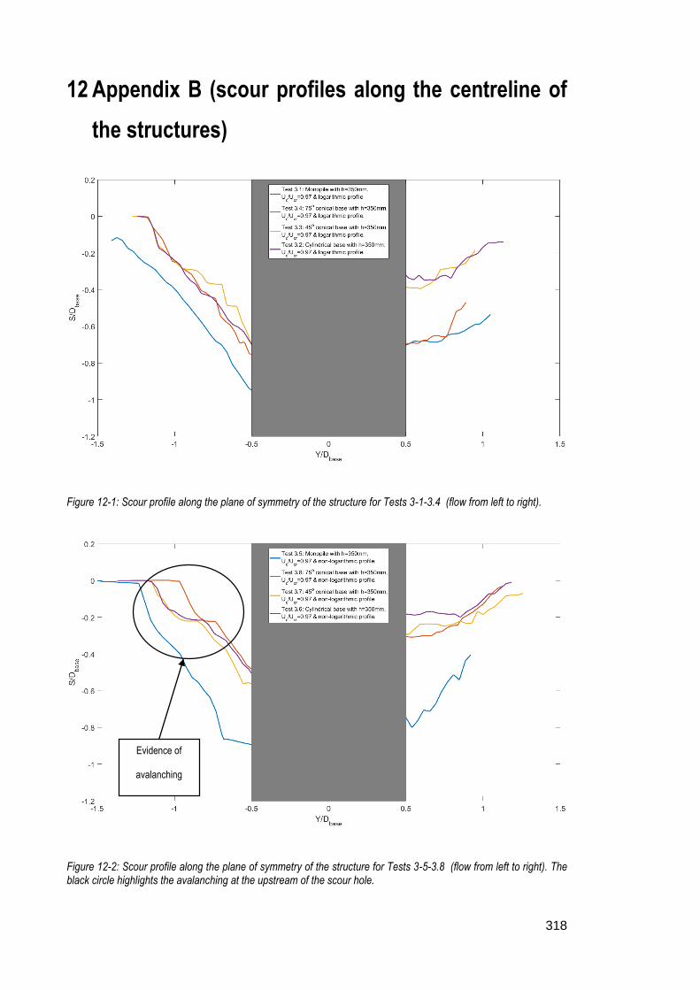
318

12 Appendix B (scour profiles along the centreline of

the structures)

Figure 12-1: Scour profile along the plane of symmetry of the structure for Tests 3-1-3.4 (flow from left to right).

Figure 12-2: Scour profile along the plane of symmetry of the structure for Tests 3-5-3.8 (flow from left to right). The black circle highlights the avalanching at the upstream of the scour hole.

Evidence of

avalanching

319



Scour and scour protection around offshore gravity based ...

Documents

Transcript of Scour and scour protection around offshore gravity based ...