An Energy Efficient Approach to Dynamic Coverage in Wireless Sensor Networks

An Energy Efficient Approach to Dynamic

Coverage in Wireless Sensor Networks

Mohamed K. Watfa Department of Computer Science, American University of Beirut, Beirut, Lebanon

[email protected]

Sesh Commuri School of Electrical and Computer Engineering, University of Oklahoma, Norman, OK, USA

[email protected]

Abstract- Tracking of mobile targets is an important

application of sensor networks. This is a non-trivial problem

as the increased accuracy of tracking results in an overall

reduction in the lifetime of the sensor network. In this

paper, the tracking issue is first addressed through the

determination of a reduced cover for the region of interest.

Tracking algorithms are then developed using a reduced set

of sensor nodes. The tradeoffs involved in the energy

efficient tracking of the target are studied and the

performance of the distributed tracking algorithms is

compared with well known strategies from the literature. It

is shown that the gain in energy savings comes at the

expense of reduced quality of tracking. The algorithms

guarantee the robustness and accuracy of tracking as well

as the extension of the overall system lifetime. Numerical

simulations are presented to validate the performance of the

proposed algorithms.

Index Terms: ad-hoc and sensor networks, tracking, 3D

coverage, energy efficiency, reduced cover.

I. INTRODUCTION

A Wireless Sensor Network (WSN) is a

computational network of many, spatially distributed

sensing devices that can be used to monitor conditions

such as temperature, sound, vibration, pressure, motion

or pollutants at various locations. Usually these devices

are small, inexpensive, and their resources in terms of

energy, memory, computational speed and bandwidth are

severely constrained [1, 2]. The application of sensor

networks in the tracking of dynamic phenomenon or

targets is an important and widely researched area in

sensor networks.

An important issue to be addressed in the ability of a

WSN to track a dynamic target is the coverage of the

WSN. Coverage in a WSN was considered by Gupta and

Das in [3]. Here, the notion of a ‘connected sensor cover’

was introduced and the energy efficiency addressed

through the construction of a near-optimal connected

sensor cover. Shakkottai [8] derived the necessary and

sufficient conditions for the connectivity and coverage in

terms of the sensing radius, transmission radius and the

failure rates of sensors. Zhang and Hou [9] show that if

the communication range is at least twice the sensing

range, then complete coverage of a convex area implies

connectivity among the nodes. A Coverage Configuration

Protocol (CCP) that can provide different degrees of

connected coverage is presented in [10].

While coverage of a region of interest is essential for

tracking using WSNs, the limited power available at each

sensor node requires the determination of a minimum set

of nodes that can guarantee coverage. The problem of

selecting a subset of randomly deployed nodes for energy

efficiency and coverage of an area was addressed in [4,

5]. The problem of selecting a minimum number of nodes

such that each node in the network is either selected or is

a neighbor of a selected node was also formulated as the

minimum dominating connected set (MDCS) problem

[6]. In [7], Chen and Liestman proposed an algorithm for

finding small weakly connected dominating sets in a

WSN. Here, energy-efficient distributed algorithms were

developed to construct a near optimal dominating

connected set. The coverage issues in three-dimensional

deployment of sensor networks was addressed in [21]

where computational geometric methods were used to

develop computationally simple, distributed algorithms

for the optimal sensor selection as well as for network

healing in the event of failures.

Tracking, which involves identifying an object by its

particular sensor signature and determining its path over

a period of time, is one of the applications that can

benefit from exploiting the characteristics of wireless

sensor networks. The inherent parallelism of distributed

sensors makes it possible to track multiple objects

simultaneously, while the relatively low cost and ease of

deployment enable the use of sensor network based

tracking systems in remote or inaccessible locations, and

when they need to be deployed on short notice. Even

Based on “An energy efficient 3-dimensional wireless sensor cover”,

by M. Watfa and S. Commuri which appeared in the Proceedings of the

IEEE CCNC 2006, Las Vegas, NV, USA, 2006. © 2006 IEEE.

10 JOURNAL OF NETWORKS, VOL. 1, NO. 4, AUGUST 2006

© 2006 ACADEMY PUBLISHER

though target tracking has been widely studied for sensor

networks with large nodes and distributed tracking

algorithms are available [11-15], tracking in ad hoc

networks with micro sensors poses different challenges

due to communication, processing and energy

constraints. In particular, the sensors should collaborate

and share data to exploit the benefits of sensor data

fusion, but this should be done without sending data

requests to and collecting data from all sensors, thus

overloading the network and using up the energy supply.

Target tracking is considered a canonical application

for wireless sensor networks, and work in this area has

been motivated in large part by DARPA programs. Zhao

et al. present the information driven sensor querying

(IDSQ) mechanism in [14, 15]. IDSQ is a sensor-to-

sensor leader handoff based scheme in which at any

given time there is a leader sensor node which makes the

decisions about which sensors should be selectively

turned on in order to obtain the best information about

the target. Liu et al. [16] develop a dual-space approach

to tracking targets which also enables selective activation

of sensors based on which nodes the target is likely to

approach next. Along these lines, Ramanathan et al. [17],

advocate a location-centric approach to performing

collaborative sensing and target tracking. The idea is to

develop programming abstractions that provide

addressing and communication between localized

geographic regions within the network rather than

individual nodes. This makes localized selective-

activation strategies simpler to implement. Brooks et al.

present self-organized distributed target tracking

techniques with prediction based on Pheromones,

Bayesian, and Extended Kalman Filter techniques [18,

19]. The implementation and testing of a real distributed

sensor network collaborative tracking algorithm in a

military context is described in [20].

In the research mentioned above, the algorithms

utilized the information from all the sensors for tracking.

This results in higher expenditure of energy and reduced

lifetime for the network. In this paper, it is demonstrated

that substantial savings can be obtained by using a

reduced number of nodes at each instant for tracking the

target. Further, it is also demonstrated that this savings

comes at the expense of the quality of tracking. The

techniques presented are computationally simple and can

be implemented in a distributed fashion.

The rest of the paper is organized as follows. The

design challenges for tracking using wireless sensor

networks are presented in Section 2. Preliminary

definitions are stated in Section 3 and an algorithm for

obtaining 3D coverage is presented in Section 4. In

Section 5, an energy efficient distributed algorithm for

tracking a dynamic phenomenon is addressed. Numerical

simulation results that validate the proposed algorithms

are presented in Section 6 and the conclusions are

summarized in Section 7.

II. PERFORMANCE ISSUES

Though certain types of energy harvesting are

conceivable, energy efficiency will be a deciding factor

in the success of WSNs in the foreseeable future. This

requirement pervades all aspects of the system's design,

and drives most of the other requirements. In this section,

some key design challenges for any proposed tracking

algorithm in the domain of wireless sensor networks is

outlined.

1. Large number of sensors: Given the large number of

sensor nodes deployed, scalability is a major issue.

Nodes may fail and new nodes may join the network.

In the light of target tracking, the coordination

function should scale with the size of the network,

the number of targets to be tracked.

2. Low energy use: Since in many applications the

sensor nodes will be deployed in a remote area,

service of a node may not be possible. In this case,

the lifetime of a node may be determined by the

battery life, thereby requiring the minimization of

energy expenditure.

3. Network self-organization: Since the network can

be randomly deployed in inaccessible regions, the

sensor nodes should be capable of organizing

themselves into a network and achieving the desired

objective in the absence of any human intervention.

4. Collaborative signal processing: The end goal is

detection/estimation of some events of interest, and

not just communications. To improve the

detection/estimation performance, it is often quite

useful to fuse data from multiple sensors.

5. Distributed processing: While a centralized

architecture is theoretically optimal and conceptually

simple [5], it is not suitable in a large scale area

because of the limited communication bandwidth of

the wireless sensors. Moreover, failure of the fixed

superior node may imply failure of the whole

system.

6. Tracking accuracy: To be effective, the tracking

system should be accurate and the likelihood of

missing a target should be low.

7. Computation and communication costs: Any

protocol being developed for sensor networks should

keep in mind the costs associated with computations

and communication. With current technology, the

cost of computation locally is lower than that of

communication in a power constrained scenario. As

a consequence, emphasis should be put on

minimizing the communication requirements.

8. Uncertainty: The exact positions of the nodes can

not be known, so any position estimate of the target

being tracked will be affected.

9. Multi-modality sensor network: A multi-modal

network can obtain more complete descriptions of

the monitored environment by combining the data

from various sensors with different capabilities and

strengths.

JOURNAL OF NETWORKS, VOL. 1, NO. 4, AUGUST 2006 11


10. Time synchronization: Time synchronization is a

critical piece of infrastructure for any distributed

system.

In this paper, these issues are addressed through the

development of a reduced cover strategy that minimizes

the number of sensor nodes that are active at any given

time. A self healing concept based on the reduced cover

was developed in [21] to address the energy efficiency,

self-organization, and reliability of the network. In this

paper, the approach in [21] is extended to the case of

distributed energy efficient tracking. The algorithm

specifically aims at minimizing the number of active

nodes necessary to track a dynamic phenomenon while

achieving a high level of tracking accuracy.

III. PRELIMINARIES

An emerging application area for sensor networks is

intelligent surveillance and tracking. In these

applications, information obtained from nodes far away

from the region of activity is of little or no use. On the

other hand, in dense WSNs, the information obtained

from some sensors close to the region of activity might

be redundant. Since the lifetime of the WSN is affected

by the availability of energy, an obvious way to conserve

energy is to switch on only a subset of the sensor nodes.

In most sensor activation strategies, energy savings come

at the expense of a reduction in the quality of tracking.

Depending on the information provided by a small subset

of the sensor nodes would result in an increased

uncertainty and thus the tracking accuracy would decline.

In this paper, a reduced cover of a region is first obtained

and energy efficient algorithms that address the issues in

section II are then developed.

One of the fundamental problems in sensor networks

is determining how many sensors nodes are required to

cover a specific area at any given time. Most existing

results focus on planar networks [3]-[7]; however, three-

dimensional modeling of the sensor network would

reflect more accurately the real-life situations [21]. We

will start by defining the notion of a sensing region of a

sensor node. Then, we provide definitions for both a

reduced cover and a border cover. These definitions will

aid in the development of a distributed tacking algorithm.

Definition 1: Let 3iY y R | O ( y ) .

The sensing region of sensor Si located at 3iX R is

defined as i i sA y Y | y X R , where ||.|| is the

Euclidean distance between y and iX .

In the case of 2D, the sensing region is assumed to be a

disk of radius sR . The sensing boundary (circle) of

sensor iS , in this case, is denoted by iCir .

Definition 2: A collection, 1 ,..., }F nC S S , of sensor

nodes is said to fully cover the region R if and only

if 1 2 ...R nA A A .

Definition 3: A cover RFC of R with sensor nodes

1 2, ,..., nS S S each with sensing radius sR and sensing

regions 1 2, ,..., nA A A is reduced if no proper subset of

RFC is a cover of R.

Definition 4: A set of sensor nodes RBC is said to be a

reduced boundary cover of a region R if p RB( )

, p Si for some Si Border ,ReducedC and no proper

subset of RBC is a boundary cover of R.

i.e. RB l l RBC S , for any S C is not a boundary cover of

R .

Using definition 4, a region is said to be boundary

covered if and only if an intruder is always detected as it

crosses the border of the region.

Definition 5: A boundary sensor node bS is a sensor

node that is on the boundary cover. A sensor nbS is said

to be a non-boundary sensor node if

,p C p Anb i

for some nbA Ai

i.e. its border

circle is completely covered by other sensors.

The coverage problem can be stated as: Given a dense

deployment of sensor nodes, find a minimum subset of

active nodes that guarantee full coverage of R.

IV. SENSOR SELECTION FOR 3D COVERAGE

In this section, an algorithm is developed where the

nodes make local decisions on whether to sleep, or join

the set of active nodes. If the sensing region of a node is

completely covered by its neighbors, then the node can

be disabled without affecting the overall coverage.

Let 0 1 2, , ,...,n nC S S S S be the set of all the sensor

nodes that cover the region R. Let the intersection of

sphere 0S and sphere iS be given by the circle iC , i.e.

0 .i iC A A The interior of the circle iC is said to be

the disc bounded by the circle iC , i.e. .i iD interior C

Definition 6: A circle iC is completely covered if the

disc bounded by the circle is completely covered, i.e.

, .1

j

np D p Ai

j

Theorem 1: Let the sensor node 0S be adjacent to sensor

nodes 1 2, , ... , nS S S and 0 , 1..k kC A A k n be the

circles of intersection. 0S is completely covered if and

only if all ' , 1..kC s k n are covered.

Proof: If 0S is completely covered, then every disc kD

in 0S is covered. Definition 3.1 then ensures that the “if”



part of the theorem holds. To show the “only if” part,

suppose that all the circles are covered but there exist

points in 0S that are not covered. If a circle kC in 0S is

completely covered, then each point ‘p’ on the disc

kD belongs to some sphere lS . Further, 0S can be seen

to be partitioned by the spherical patches obtained by the

intersection of the surfaces of the spheres 1 2, , ... , nS S S

in 0S . If a circle is completely covered then each

spherical segment adjacent to it is also covered. Each

spherical segment must be bounded by some circle

segment, and since each circle Ci is completely covered

then all spherical segments are also completely covered.

The utility of Theorem 3.2 is in reducing the

coverage of sensor node 0S to a simpler problem of

checking if all the circles of intersection between 0S and

the adjacent nodes are covered. This still is a complex

task that is difficult to achieve in real time. The following

theorem demonstrates a technique where such coverage

can be determined by a few straightforward

computations.

Theorem 2: A circle 0C is completely covered by

spheres if all the intersection points

, , 1...0

C C D i j ni jare covered by one or more

adjacent spheres.

Proof: Consider an uncovered point ‘p’ in 0D . Since

some parts of 0D are covered by adjacent sensor nodes,

these spheres are going to partition 0D into regions

bounded by arcs from the boundary of 0C and/or arcs

from circles 1kC ' s, k ,..,n. Suppose ‘p’ belongs to a

region xR in 0D . Since ‘p’ is not covered, is easy to see

that xR has to be bounded only by the exterior arcs of the

circles. Also, the entire boundary of xR , including the

intersection points of the arcs, must have the same

coverage status as ‘p’, i.e. all the intersection points on

the boundary of xR in 0D must not be covered. This

contradicts the assumption that all the intersection points

, , 1...0

C C D i j ni j are covered. Therefore, if all

the intersection points 0

C C Di jare covered by one

or more adjacent spheres, then 0D is covered.

Consequently, 0C is covered.

A. Algorithm for Obtaining Complete Coverage in 3-

Dimensional Space

Theorems 1 and 2 indicate that a sensor node is

completely covered if all the intersection points

i j kC C D are covered by some sensor node

1lS ,l i, j ,k ..n . Therefore, to check if 0S is

completely covered; one has to first find all the circles

obtained by the intersection of 0 , 1..kS S k n . For

each kC , find all the intersection points that lie

within kD . If all these intersection points are covered,

then the circles kC are covered. Then, by the theorems 1-

2, 0S is covered and can be deactivated.

Definition 7: A node iS is said to be a neighbor of node

jS if and only if ( , ) 2 ,i j cd X X R where cR is the

communication radius of sensor nodes iS , jS .

Definition 8: The neighbor set ( )N i of sensor node iS is

the set of all the neighbors of node iS and is defined

as ( ) { | ( , ) 2 }j i j cN i S C d X X R .

Distributed 3D Coverage Algorithm

Step 1: For each node iS , form the set of neighbors

( )N i . For each element ‘ kS ’ in ( )N i compute the

volume of overlap, ikV , between sensor node iS and kS .

If the total overlap between iS and its neighbors is less

than the volume of iS , then iS is not completely covered

by its neighbors and must remain active. That is

3

1

4

3

n

overlap ik s ik

V V R S remains active.

Step 2: 34

3overlap sV R does not necessarily mean that

iS is covered. To check if iS is covered, for every pair of

nodes inj kS ,S N i do the following:

a) Find ijC the circle got by the intersection of the

coverage surface of iS , jS .

b) Find ikC the intersection circle of i kS , S .

c) Find the intersection points ij ikC C .

d) If the intersection points are all covered, i.e.

ij ik l lC C A , S N i , l i, j ,k , then

deactivate iS .

It is well known that the coverage problem in WSNs

is NP-hard [17]. The computational complexity of the

algorithm developed in this section is 3( )N where

1

n

iN max N( i ) is the maximum number of nodes in

the neighbor set of any sensor in the network.

V. DISTRIBUTED TRACKING ALGORITHM

In the previous section, and algorithm for selecting a

reduced set of sensor nodes in order to cover a 3D region

was presented. In this section, our results from the



previous section will be used to develop an energy

efficient distributed tracking algorithm using the

minimum subset of sensor nodes.

A. Algorithms

The objective of the intrusion detection algorithm is

to achieve a static arrangement of the sensor nodes that

minimizes the probability of undetected penetration of

the intruder. It will first be shown that if there exists a

reduced cover of a region of interest, then the border

cover (minimum set of sensor nodes that cover the

boundary of a region) is a subset of the reduced cover.

A sensor iS is not on the boundary of coverage (or

coverage hole H) if and only if its sensing boundary

circle iCir is completely covered by its neighbors i.e.

i i j jS B( H ) p Cir , p A , for some S S . Now,

the boundary of coverage (or coverage hole H) can be

defined in terms of the set of sensor nodes.

Lemma 3: Every reduced cover reducedC of a region R

admits a border cover borderC such that .border reducedC C

Proof:

Let | .b k k reduced kC S S C and A B R

Then, , .k k bk

x B R x A where S C This implies

that bC is a cover for the border of the region and by

construction, .b reducedC C

Lemma 3 is a powerful result as it enables the

selection of sensor nodes to cover the boundary of a

region as a subset of the reduced cover of the region.

Tracking algorithms based on the reduced cover employ

fewer nodes and are therefore efficient from an energy

standpoint. Activating only those nodes in the vicinity of

the target being tracked also reduces the energy

consumption of the network. This can be accomplished

by activating the sensor nodes in the vicinity of the

sensor node that has detected the target. The radius of the

active zone depends on the maximum speed of the

intruder and the maximum time needed to calculate a

reduced cover. The key to the algorithm is that there is no

central controller i.e. each node will decide

autonomously to be active or not in order to track the

target.

The sensor nodes in the network can be in three

different modes:

1- Active Mode: A node is capable of both sensing and

communicating with neighboring nodes.

2- Relay Mode: A node can only communicate with

neighbors.

3- Sleep Mode: A node is inactive.

The tracking algorithms in this paper depend on the

idea of “Divide and Conquer” where at each instant a

reduced sensor cover is established for the moving zone.

When a sensor node on the boundary detects that the

target is about to leave the zone, a new zone is created

with the border sensor node as its center. A set of new

sensor nodes are then activated. In a refinement of this

algorithm, prediction techniques are utilized to activate a

subset of the nodes in the reduced cover depending on

the predicted location of the target. Both approaches are

discussed in details in the following sections.

Next, we will provide a number of algorithms that

will aid us in developing a distributed tracking algorithm.

Algorithm 1 (Reduced Cover Algorithm)

PROBLEM

Given a dense deployment of sensor nodes, find a

minimum subset of active nodes that guarantee full

coverage of R.

SOLUTION

The distributed coverage algorithm developed in Section

4 is used.

Algorithm 2 (Sub Reduced Cover Algorithm)

PROBLEM

Given a reduced cover set of a region R, deduce the

reduced cover of a sub region Rsub of R.

SOLUTION

Each node ( , , )j j j jS x y z that is part of the reduced

cover set will receive an ALERT message that contains

the coordinates of the center of the sub region

( , , )i i i iS x y z and the maximum speed of the intruder. A

node jS will be added to the sub-cover if

max max( , ) .i jd S S V t .

Algorithm 3 (Boundary Cover Algorithm)

PROBLEM

Given a reduced cover set of a region R, deduce the

border cover.

SOLUTION

Each node ( , , )j j j jS x y z that is a part of the reduced

cover set will receive an ALERT message that contains

the coordinates of the center of the sub region

( , , )i i i iS x y z and the maximum speed of the intruder and

therefore can deduce the radius subr of the sub region. jS

will be added to the reduced sub-cover if

( , )sub s i j sub sr R d S S r R .

Algorithm 4 (Prediction Algorithm)

In the linear prediction (LP) model, also known as the

autoregressive (AR) model, the next location X(n) is

approximated by a linear combination of k past

locations. We are then looking for a vector ‘a’ of k

coefficients, k being the order of the LP model. Provided



that the ‘a’ is estimated, the predicted value is computed

simply by FIR filtering of the k past samples with the

coefficients using1

( ) ( )k

ii

X n a X n i . To keep the

calculation simple and the communication overhead low,

the prediction model we use is only based on the target’s

moving speed and its direction of movement using the

previous and current position of the target to predict the

next location. The previous position of the target

( ) ( ( ), ( ))X t a x t a y t a and the current position of

the target ( ) ( ( ), ( ))X t x t y t are used to estimate the

velocity and the direction of the movement. The velocity

is given by ( ( ), ( ))d X t X t a

va

while the direction

is 1 ( ) ( )cos

( ( ), ( ))

x t x t a

d X t X t a. The next position of the

target can be predicted by ( ) ( ) cosx t a x t vt

and ( ) ( ) siny t a y t vt .

B. Tracking Algorithm

Energy efficient tracking of a target involves

different steps:

Phase 1:

Find a reduced cover of the region of interest.

Deduce the border cover of the region of interest.

Phase 2:

Detect the presence of the target.

Broadcast the coordinates of the border sensor node

and activate the necessary Sub reduced cover

(Deduce the Sub border Cover).

Move the sub region accordingly.

The distributed tracking algorithm works by

assigning a role for each sensor node. The initialization

phase basically activates a border cover of the region of

interest i.e. all the sensor nodes on the border of the

region of interest are active. When a target is detected by

a particular border sensor node Si, then Si is selected as

the center node and broadcasts its coordinates to the

reduced cover nodes in order to activate a subset of the

reduced cover that will cover the sub circular zone of

center Si. The new sub border cover is deduced and as

soon as a border sensor node detects the intruder, the

same steps are repeated. This procedure guarantees the

tracking of the target at all times since the radius of the

circular zone depends on the maximum speed of the

target and on the maximum time it takes to form the

reduced cover of the sub region. A snapshot of the

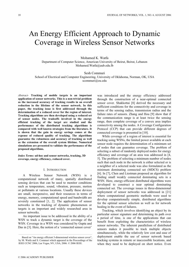
tracking algorithm is depicted in Figure 1.

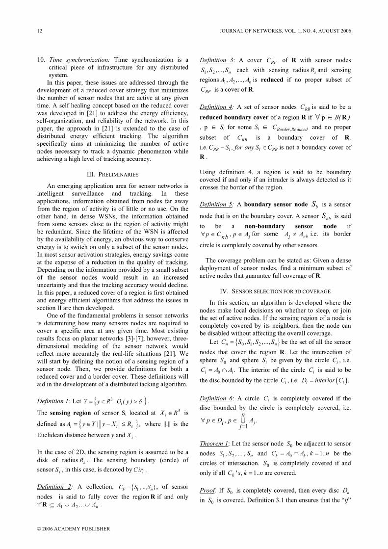
The flowchart of the processing performed at any

given node Si located at Xi to allow distributed target

tracking is provided in Figure 2.

C. Tracking Algorithm with Prediction

Figure 1. A snapshot of the distributed tracking algorithm in action.

Using the prediction algorithm, a sensor node

estimates the targets next location moving with a velocity

V and direction . Since the ultimate goal is conserve

energy while achieving the necessary tracking

performance, only a subset of the sensor nodes within a

circle of radius R=V.T and center X is activated. Since

the direction of motion is known, any sensor node that

belongs to the reduced cover and is within a circular

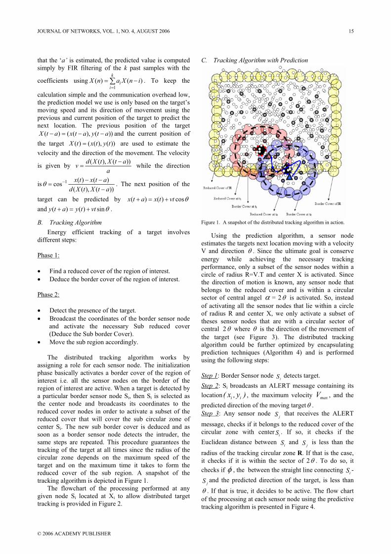
sector of central angel = 2 is activated. So, instead

of activating all the sensor nodes that lie within a circle

of radius R and center X, we only activate a subset of

theses sensor nodes that are with a circular sector of

central 2 where is the direction of the movement of

the target (see Figure 3). The distributed tracking

algorithm could be further optimized by encapsulating

prediction techniques (Algorithm 4) and is performed

using the following steps:

Step 1: Border Sensor node iS detects target.

Step 2: Si broadcasts an ALERT message containing its

location i i( x , y ) , the maximum velocity maxV , and the

predicted direction of the moving target .

Step 3: Any sensor node jS that receives the ALERT

message, checks if it belongs to the reduced cover of the

circular zone with centeriS . If so, it checks if the

Euclidean distance between iS and

jS is less than the

radius of the tracking circular zone R. If that is the case,

it checks if it is within the sector of 2 . To do so, it

checks if , the between the straight line connecting iS -

jS and the predicted direction of the target, is less than

. If that is true, it decides to be active. The flow chart

of the processing at each sensor node using the predictive

tracking algorithm is presented in Figure 4.



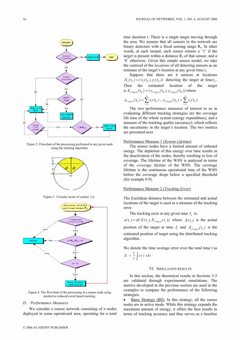
Figure 2. Flowchart of the processing performed at any given node

using the tracking algorithm.

Figure 3. Circular sector of central 2

Figure 4. The flowchart of the processing at a sensor node using

predictive reduced cover based tracking.

D. Performance Measures

We consider a sensor network consisting of n nodes

deployed in some operational area, operating for a total

time duration t. There is a single target moving through

the area. We assume that all sensors in the network are

binary detectors with a fixed sensing range Rs. In other

words, at each instant, each sensor returns a ’1’ if the

target is present within a distance Rs of that sensor, and a

’0’ otherwise. Given this simple sensor model, we take

the centroid of the locations of all detecting sensors as an

estimate of the target’s location at any given time ti.

Suppose that there are k sensors at locations

0 0 0i i iX ( t ) ( x ( t ), y ( t )) detecting the target at time 0t .

Then the estimated location of the target

is0 0 0T arg et T arg et T arg etX ( t ) ( x ( t ), y ( t )) where

0 0

1

k

T arg et i

i

x ( t ) x ( t ) , 0 0

1

k

T arg et i

i

y ( t ) y ( t )

The two performance measures of interest to us in

evaluating different tracking strategies are the coverage

life time of the whole system (energy expenditure), and a

measure of the tracking quality (accuracy), which reflects

the uncertainty in the target’s location. The two metrics

are presented next.

Performance Measure 1 (System Lifetime)

The sensor nodes have a limited amount of onboard

energy. The depletion of this energy over time results in

the deactivation of the nodes, thereby resulting in loss of

coverage. The lifetime of the WSN is analyzed in terms

of the coverage lifetime of the WSN. The coverage

lifetime is the continuous operational time of the WSN

before the coverage drops below a specified threshold

(for example 0.9).

Performance Measure 2 (Tracking Error)

The Euclidean distance between the estimated and actual

locations of the target is used as a measure of the tracking

error.

The tracking error at any given time it is:

i i T arg et ie( t ) d( X( t ),X ( t )) where iX( t ) is the actual

position of the target at time it andT arg et iX ( t ) is the

estimated position of target using the distributed tracking

algorithm.

We denote the time average error over the total time t as

0

1t

E e ( t )d tt

.

VI. SIMULATION RESULTS

In this section, the theoretical results in Sections 3-5

are validated through experimental simulations. The

metrics developed in the previous section are used in the

examples to compare the performance of the following

strategies.

Basic Strategy (BS): In this strategy, all the sensor

nodes are in active mode. While this strategy expends the

maximum amount of energy, it offers the best results in

terms of tracking accuracy and thus serves as a baseline



for comparison with the strategies developed in Section

5.

Basic Selective Predictive Strategy (BSPS): In this

strategy, only the nodes in the vicinity of the target are

activated for tracking. These nodes also predict the

“next” position of the target and hand over tracking to

nodes best placed to track the target. The remaining

nodes are in “relay” mode and can switch to tracking

mode on being alerted by the tracking nodes.

Reduced Cover Strategy (RCS): In this strategy,

only the sensor nodes in the reduced cover obtained

using Algorithm 1 are used to track the object. In contrast

to the Basic Strategy, complete coverage of the region is

still maintained, but by using the reduced cover.

Reduced Cover Selective Tracking Strategy

(RCSTS): In this strategy, a subset of all the sensor nodes

in the reduced cover is activated to track the target while

the rest of the nodes are in the relay mode.

Reduced Cover Selective Predictive Strategy

(RCSPS): In this approach, the subset of nodes in the

vicinity of the target is determined using Algorithm 4.

Here, instead of waking up all the nodes in the vicinity of

the target, those nodes belonging to a sector determined

by the current position and velocity of the target are

activated.

In the following examples, 2000 nodes, each with a

sensing radius of 1 unit, are assumed to be uniformly

randomly deployed in a region of size 10x10x10 units

(Figure 5). Each sensor node is also assumed to have a

limited energy supply (300 Joules) and is deactivated

when the energy is depleted. The power consumption of

Tx (transmit), Rx (receive), Idle and Sleeping modes are

1400mW, 1000mW, 830mW, 130mW respectively.

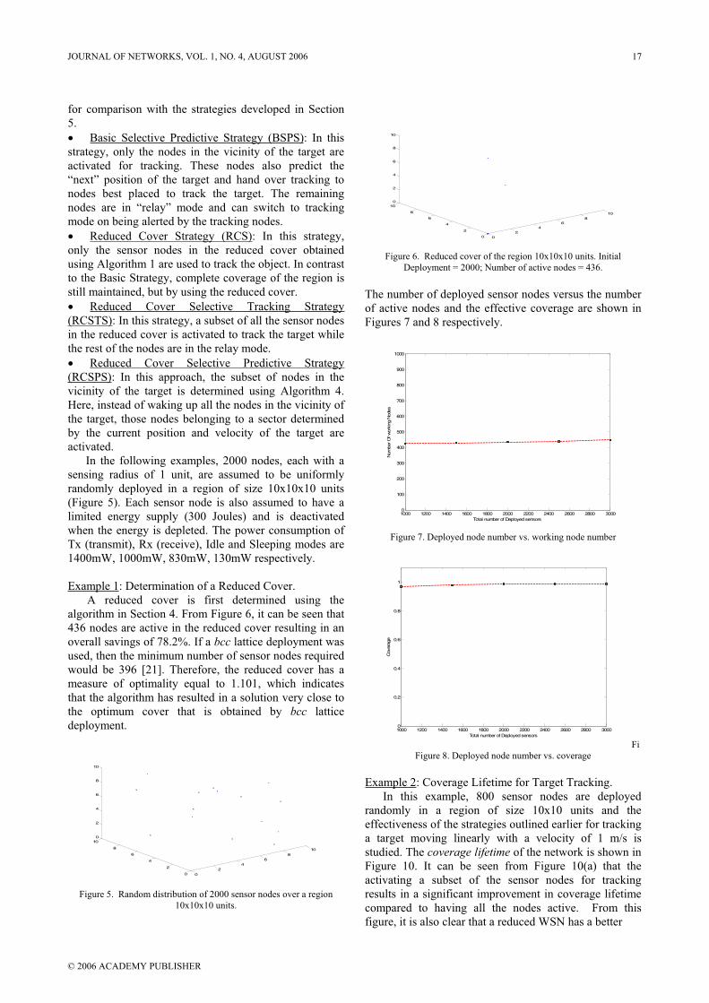
Example 1: Determination of a Reduced Cover.

A reduced cover is first determined using the

algorithm in Section 4. From Figure 6, it can be seen that

436 nodes are active in the reduced cover resulting in an

overall savings of 78.2%. If a bcc lattice deployment was

used, then the minimum number of sensor nodes required

would be 396 [21]. Therefore, the reduced cover has a

measure of optimality equal to 1.101, which indicates

that the algorithm has resulted in a solution very close to

the optimum cover that is obtained by bcc lattice

deployment.

0

24

68

10

0

2

4

6

8

100

2

4

6

8

10

Figure 5. Random distribution of 2000 sensor nodes over a region

10x10x10 units.

0

24

68

10

0

2

4

6

8

100

2

4

6

8

10

Figure 6. Reduced cover of the region 10x10x10 units. Initial

Deployment = 2000; Number of active nodes = 436.

The number of deployed sensor nodes versus the number

of active nodes and the effective coverage are shown in

Figures 7 and 8 respectively.

1000 1200 1400 1600 1800 2000 2200 2400 2600 2800 30000

100

200

300

400

500

600

700

800

900

1000

Total number of Deployed sensors

Num

ber O

f w

orki

ng N

odes

Figure 7. Deployed node number vs. working node number

1000 1200 1400 1600 1800 2000 2200 2400 2600 2800 30000

0.2

0.4

0.6

0.8

1

Total number of Deployed sensors

Cov

erag

e

Fi

Figure 8. Deployed node number vs. coverage

Example 2: Coverage Lifetime for Target Tracking.

In this example, 800 sensor nodes are deployed

randomly in a region of size 10x10 units and the

effectiveness of the strategies outlined earlier for tracking

a target moving linearly with a velocity of 1 m/s is

studied. The coverage lifetime of the network is shown in

Figure 10. It can be seen from Figure 10(a) that the

activating a subset of the sensor nodes for tracking

results in a significant improvement in coverage lifetime

compared to having all the nodes active. From this

figure, it is also clear that a reduced WSN has a better



(a)

(b)

(c)

(d)Figure 9. (a),(c) The coverage life time of the network as time passes

using algorithms BS, RCS, BSPS when the number of deployed nodes

is 800 and 1600 respectively. (b), (d). The coverage life time of the

network as time passes using algorithms BSPS, RCSTS, RCSPS when

the number of deployed nodes is 800 and 1600 respectively.

Figure 10. The resulting tracking error as we increase the sensing

radius of each sensor node using 4 different algorithms: BS, BSPS,

RCSTS, and RCSPS.

coverage lifetime over the full network. This

improvement, however, comes at a price. The algorithm

for obtaining the reduced network requires the

communication between a node and its neighbors and as

a result a portion of energy is used up during the

initialization stage of the network. This causes early

onset of degradation and loss of cover. This, however,

can be addressed by incorporating self healing in the

WSN [21].

The two tracking algorithms (RCSTS and RCSPS)

proposed earlier can further improve the energy savings

and thus increasing the overall cover life time of the

system (Figure 9(a),(b)). Similar results are observed as

the number of deployed sensor nodes is increased.

However, using BSPS decreases the performance since

all the sensor nodes within a specified radius are active in

the reduced cover approach, the number of sensor nodes

to be activated would almost be the same since we first

calculate the reduced cover of the region and then

activate the necessary subset in order to track the target.

The results are shown in Figure 9(c) and Figure 9(d).

Example 3: Comparison of Tracking Error.

In this example, the accuracy of the different tracking

algorithms is studied. We notice that in terms of tracking

error, with no surprise, BS outperforms all the others.

However, as the sensing radius of each sensor node is

increased, all the other algorithms converge to a

negligible tracking error. The results are shown in Figure

10.

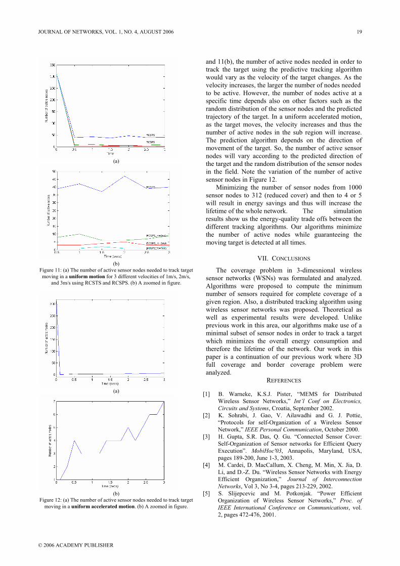
Example 4: Comparison of Performance.

In this example, the performance of the WSN in

tracking a target moving along a trajectory of the

form by( t ) ax ( t ) c sin dx( t ) e is studied. Using the

basic strategy, 312 (Reduced Cover) nodes are always

active. Using RCSTS, the size of the sub region depends

on the maximum velocity of the target and thus the

number of nodes that will be activated would not vary as

we change the velocity. As can be seen in Figures 11(a)



(a)

(b)

Figure 11: (a) The number of active sensor nodes needed to track target

moving in a uniform motion for 3 different velocities of 1m/s, 2m/s,

and 3m/s using RCSTS and RCSPS. (b) A zoomed in figure.

(a)

(b)

Figure 12: (a) The number of active sensor nodes needed to track target

moving in a uniform accelerated motion. (b) A zoomed in figure.

and 11(b), the number of active nodes needed in order to

track the target using the predictive tracking algorithm

would vary as the velocity of the target changes. As the

velocity increases, the larger the number of nodes needed

to be active. However, the number of nodes active at a

specific time depends also on other factors such as the

random distribution of the sensor nodes and the predicted

trajectory of the target. In a uniform accelerated motion,

as the target moves, the velocity increases and thus the

number of active nodes in the sub region will increase.

The prediction algorithm depends on the direction of

movement of the target. So, the number of active sensor

nodes will vary according to the predicted direction of

the target and the random distribution of the sensor nodes

in the field. Note the variation of the number of active

sensor nodes in Figure 12.

Minimizing the number of sensor nodes from 1000

sensor nodes to 312 (reduced cover) and then to 4 or 5

will result in energy savings and thus will increase the

lifetime of the whole network. The simulation

results show us the energy-quality trade offs between the

different tracking algorithms. Our algorithms minimize

the number of active nodes while guaranteeing the

moving target is detected at all times.

VII. CONCLUSIONS

The coverage problem in 3-dimesnional wireless

sensor networks (WSNs) was formulated and analyzed.

Algorithms were proposed to compute the minimum

number of sensors required for complete coverage of a

given region. Also, a distributed tracking algorithm using

wireless sensor networks was proposed. Theoretical as

well as experimental results were developed. Unlike

previous work in this area, our algorithms make use of a

minimal subset of sensor nodes in order to track a target

which minimizes the overall energy consumption and

therefore the lifetime of the network. Our work in this

paper is a continuation of our previous work where 3D

full coverage and border coverage problem were

analyzed.

REFERENCES

[1] B. Warneke, K.S.J. Pister, “MEMS for Distributed

Wireless Sensor Networks,” Int’l Conf on Electronics,

Circuits and Systems, Croatia, September 2002.

[2] K. Sohrabi, J. Gao, V. Ailawadhi and G. J. Pottie,

“Protocols for self-Organization of a Wireless Sensor

Network,” IEEE Personal Communication, October 2000.

[3] H. Gupta, S.R. Das, Q. Gu. “Connected Sensor Cover:

Self-Organization of Sensor networks for Efficient Query

Execution”. MobiHoc'03, Annapolis, Maryland, USA,

pages 189-200, June 1-3, 2003.

[4] M. Cardei, D. MacCallum, X. Cheng, M. Min, X. Jia, D.

Li, and D.-Z. Du. “Wireless Sensor Networks with Energy

Efficient Organization,” Journal of Interconnection

Networks, Vol 3, No 3-4, pages 213-229, 2002.

[5] S. Slijepcevic and M. Potkonjak. “Power Efficient

Organization of Wireless Sensor Networks,” Proc. of

IEEE International Conference on Communications, vol.

2, pages 472-476, 2001.



[6] S. Guha and S. Khuller. “Approximation algorithms for

connected dominating sets.” Proc. of 4th Annual European

Symposium on Algorithms, pages 179-193, 1996.

[7] Y. Chen and A. Liestman. “Approximating minimum size

weakly-connected dominating sets for clustering mobile ad

hoc networks.” In Proc. of the Symp. On Mobile ad hoc

networking and computing, pages 165-172, June 2002.

[8] S. Shakkottai, R. Srikant, and N. Shro. “Unreliable sensor

grids: Coverage, connectivity and diameter.” In

Proceedings of INFOCOM, pages 1073-1083, 2003.

[9] H. Zhang and J. C. Hou, “Maintaining Sensing Coverage

and Connectivity in Large Sensor Networks,” Technical

Report UIUC, UIUCDCS-R-2003-2351, 2003.

[10] W. R. Heinzelman, A. Chandrakasan, and H.

Balakrishnan. “Energy-efficient communication protocol

for wireless micro sensor networks.” In Proc. Of Intl.

Conf. on System Sciences (HICSS), pages 1-10, 2000.

[11] C. Meesookho, S. Narayanan, and C.S. Raghavendra,

Collaborative Classification Applications in Sensor

Networks, Sensor Array and Multichannel Signal

Processing Workshop, August 2002.

[12] D. Li, K.D. Wong, Y.H. Hu, and A.M. Sayeed, Detection,

classification, and tracking of targets, IEEE Signal

Processing Magazine, March 2002.

[13] Q. Fang, F. Zhao, and L. Guibas, Counting Targets:

Building and Managing Aggregates in Wireless Sensor

Networks, Xerox Palo Alto Research Center (PARC)

Technical Report, June 2002.

[14] M. Chu, H. Haussecker, and F. Zhao, Scalable

Information-Driven Sensor Querying and Routing for ad

hoc Heterogeneous Sensor Networks, Xerox Palo Alto

Research Center (PARC), July 2001.

[15] F. Zhao, J. Shin, J. Reich, “Information-Driven Dynamic

Sensor Collaboration for Tracking Applications.” IEEE

Signal Processing Magazine, March 2002.

[16] J. Liu, P. Cheung, L. Guibas, and F. Zhao, A Dual-Space

Approach to Tracking and Sensor Management in Wireless

Sensor Networks, Palo Alto Research Center, Technical

Report P2002-10077, March 2002.

[17] P. Ramanathan, Location-centric Approach for

Collaborative Target Detection, Classification, and

Tracking, IEEE CAS Workshop on Wireless

Communication and Networking, September 2002.

[18] R. Brooks, and C. Griffin, “Traffic model evaluation of ad

hoc target tracking algorithms,” Journal of High

Performance Computer Applications, Accepted, 2002.

[19] R. Brooks, C. Griffin, and D. S. Friedlander, “Self-

Organized distributed sensor network entity tracking,”

International Journal of High Performance Computer

Applications, special issue on Sensor Networks, vol. 16,

no. 3, Fall 2002.

[20] J. Moore, T. Keiser, R. R. Brooks, S. Phoha, D.

Friedlander, J. Koch, A. Reggio, and N. Jacobson,

“Tracking Targets with Self-Organizing Distributed

Ground Sensors,” 2003 IEEE Aerospace Conference,

Invited Paper, Accepted for publication, November 2002.

[21] Watfa M., Commuri S., “An Energy Efficient and Self-

Healing 3-Dimensional Sensor Cover”, International

Journal of Ad Hoc and Ubiquitous Computing (IJAHUC),

2006 (to appear).

Mohamed K. Watfa is an Assistant Professor in the

department of Computer Science at the American University of

Beirut. He received his Ph.D. from the School of Electrical and

Computer Engineering at the University of Oklahoma in

Norman, OK in 2006. He obtained his BS in Computer Science

from American University of Beirut in 2002 and his Masters

degree in Engineering Science from the University of Toledo,

OH in 2003. His research interests include sensor networks,

wireless networking, software engineering, resource

management, energy issues, tracking, routing, and performance

measures. He is also a member of the ACM and IEEE.

Sesh Commuri is an Associate Professor in the School of

Electrical and Computer Engineering at the University of

Oklahoma in Norman. He received his Masters degree in

Electrical Engineering from the Indian Institute of Technology,

Kanpur, India in 1989 and Ph. D in Electrical Engineering from

the University of Texas at Arlington in 1996. Dr. Commuri has

over 9 years experience in the industry and his research

interests include wireless sensor networks, intelligent systems,

real-time systems, mechatronics, embedded controls and

robotics.



An Energy Efficient Approach to Dynamic Coverage in Wireless Sensor Networks

Documents

Transcript of An Energy Efficient Approach to Dynamic Coverage in Wireless Sensor Networks