An efficient numerical technique for solving population balance equation involving aggregation,...

Available online at www.sciencedirect.com

(2008) 81–104www.elsevier.com/locate/powtec

Powder Technology 182

An efficient numerical technique for solving population balance equationinvolving aggregation, breakage, growth and nucleation

Jitendra Kumar a,⁎, Mirko Peglow b, Gerald Warnecke a, Stefan Heinrich c

a Institute for Analysis and Numerics, Otto-von-Guericke University Magdeburg, Universitätsplatz 2, D-39106 Magdeburg, Germanyb Institute for Process Engineering, Otto-von-Guericke University Magdeburg, Universitätsplatz 2, D-39106 Magdeburg, Germany

c Institute of Process Equipment and Environmental Technology, Otto-von-Guericke University Magdeburg,Universitätsplatz 2, D-39106 Magdeburg, Germany

Received 27 February 2007; received in revised form 29 May 2007; accepted 30 May 2007Available online 6 June 2007

Abstract

Anew discretization for simultaneous aggregation, breakage, growth and nucleation is presented. The new discretization is an extension of the cellaverage technique developed by the authors [J. Kumar, M. Peglow, G. Warnecke, S. Heinrich, and L. Mörl. Improved accuracy and convergence ofdiscretized population balance for aggregation: The cell average technique. Chemical Engineering Science 61 (2006) 3327–3342.]. It is shown thatthe cell average scheme enjoys the major advantage of simplicity for solving combined problems over other existing schemes. This is done by aspecial coupling of the different processes that treats all processes in a similar fashion as it handles the individual process. It is demonstrated that thenew coupling makes the technique more useful by being not only more accurate but also computationally less expensive. At first, the coupling isperformed for combined aggregation and breakage problems. Furthermore, a new idea that considers the growth process as aggregation of existingparticle with new small nuclei is presented. In that way the resulting discretization of the growth process becomes very simple and consistent with firsttwo moments. Additionally, it becomes easy to combine the growth discretization with other processes. The new discretization of pure growth is alittle diffusive but it predicts the first twomoments exactly without any computational difficulties like appearance of negative values or instability etc.The numerical scheme proposed in this work is consistent only with the first two moments but it can easily be extended to the consistency with anytwo or more than two moments. Finally, the discretization of pure and coupled problems is tasted on several analytically solvable problems.© 2007 Elsevier B.V. All rights reserved.

Keywords: Population balance; Aggregation; Breakage; Growth; Nucleation ; Particle; Batch

1. Introduction

In particle technologies population balance equations arewidely used, e.g. in processes such as crystallization, commi-nution and fluidized bed granulation. They appear also inmathematical biology as well as in aerosol science. These arepartial integro-differential equations of hyperbolic or parabolictype. Included are conservation laws with integral fluxes. Inde-pendent variables are particle properties, especially particle size,over which a particle number distribution is considered forwhich the population balance is formulated. Analytical solutions

⁎ Corresponding author. Tel.: +49 391 6711629; fax: +49 391 6718073.E-mail address: [email protected] (J. Kumar).

0032-5910/$ - see front matter © 2007 Elsevier B.V. All rights reserved.doi:10.1016/j.powtec.2007.05.028

are available only for a limited number of simplified problemsand therefore numerical solutions are frequently needed to solvea population balance system.

Several numerical techniques including the method of succes-sive approximations [40], the method of moments [3,28,31], thefinite elements methods [29,33,41], the finite volume scheme[6–9,32,48] and Monte Carlo simulation methods [19,25,26,44]can be found in the literature for solving population balanceequations. Besides the approximation of the particle propertydistribution, a correct prediction of some selected propertiessuch as the total number of particles and total mass etc. is mainlyrequired in many particulate systems. These requirements lead tothe choice of sectional methods. The sectional methods approx-imate the continuous size distribution by a finite number ofsize sections (intervals, cells). A system of ordinary differential

http://dx.doi.org/10.1016/j.powtec.2007.05.028

mailto:[email protected]

82 J. Kumar et al. / Powder Technology 182 (2008) 81–104

equations describing the change of the number of particles ineach cell is usually obtained and then using any higher ordertime integrator is solved. The accuracy of the method certainlydepends on the number of cells. Such methods rely on predictingsome selected properties of the distribution exactly rather thancapturing all details of the distribution. Moreover, simplicity andlow computational cost of these methods make them highlypractical in process engineering.

There are several sectional methods in the literature whichpredict the particle property distribution accurately while using alinear grid, see for example Sutugin and Fuchs [46], Tolfo [47],Kim and Seinfeld [15], Gelbard et al. [10], Sastry andGaschignard [42] as well as Marchal et al. [30]. Linear griddiscretization has a great advantage especially in aggregationproblems since each aggregate finds a new position for itsallocation. This discretization does however have one problemof extremely high computational cost due to the requirement ofexcessively many cells to cover the property domain. Instead, ageometric type discretization is commonly used to reduce thecomputational cost. The difficulty that arises in a non-uniformgrid is, where to allocate newborn particles which do not haveexactly the size of the grid point. Several authors proposeddifferent methods which can be used using geometric, Gillette[11], Batterham et al. [5], Marchal et al. [30], Hounslow et al.[13], or arbitrary grid, Kim and Seinfeld [15], Gelbard et al. [10],Sastry and Gaschignard [42], Marchal et al. [30], Kumar andRamkrishna [22]. Batterham et al. [5] produced numericalresults for aggregation that correctly predicted conservation oftotal particles volume but failed to predict the correct evolutionof total numbers. On the other hand, Gelbard et al. [10] predictedthe rate of change of total particle number correctly but lost totalparticle volume. Nonetheless, Hounslow et al. [13] have beenthe first in the literature to produce a population balance schemethat correctly predicts the total number and total volume ofparticles. They have considered a geometric discretization with afactor of 2 progression in size. This has the drawback that onecannot refine the grid. Afterwards, Litster et al. [27] haveextended the technique for adjustable geometric discretizationswith a progression factor of 21/q, where q is an integer greaterthan or equal to 1. It has been investigated by Wynn [49] that theextended formulation is valid only for qb4. Since then, Wynnhas corrected the formulation. The complex structure of theformulation and its restriction to specified grids are the majordisadvantages of this method. Wynn [50] has also presented amore simplified form of Hounslow's discretization to improvesome computational aspects. An evaluation of the varioussectional methods can be found in [4,17,18,34].

The first general formulation consistent with the first twomoments has been proposed as the so called fixed pivottechnique by Kumar and Ramkrishna [22]. The formulationtakes the form of Hounslow's formulation when applied on thegeometric grid with a factor of 2 progression in size. It uses pointmasses at a representative location in each cell. Despite the factthat the numerically calculated moments are fairly accurate, thefixed pivot technique consistently over-predicts the results ofparticle property distribution. The technique focuses on anaccurate calculation of some selected moments instead of

calculation of the whole particle property distribution. However,the fixed pivot technique can only be applied for aggregation andbreakage problems. The authors have proposed a completelydifferent concept for combined processes of aggregation orbreakage where additionally growth and nucleation are present.Nonetheless, in this work we test the performance of the newscheme by comparing the numerical results calculated by thefixed pivot technique.

Some of the existing methods overestimate the numericalresults while others are inconsistent with moments. Moreover, ofthe existing sectional methods none can be implemented forsolving combined processes effectively. We wish to have ageneral, accurate, easy to use, computationally less expensiveand simple scheme. By these standards, none of the previousschemes we know of are completely satisfactory, although someare much better than others. This leads to a clear motivation forthe development of the new scheme. Thereby the objective ofthis work is to develop a general and simple scheme whichpreserves all advantages of the existing schemes and can be usedto solve all processes simultaneously.

A general one-dimensional PBE for a well mixed system isgiven as in [12,36]

∂nðt; xÞ∂t

¼ Qin

Vnin xð Þ � Qout

Vnout xð Þ � ∂½Gðt; xÞnðt; xÞ�

∂xþ Bnuc t; xð Þ þ Bagg t; xð Þ � Dagg t; xð Þþ Bbreak t; xð Þ � Dbreak t; xð Þ: ð1Þ

Here the aggregation and breakage terms are given as follows

Bagg t; xð Þ ¼ 12

Z x

0b t; x� ϵ; ϵð Þn t; x� ϵð Þn t; ϵð Þdϵ;

Dagg t; xð Þ ¼ n t; xð ÞZ l

0b t; x; ϵð Þn t; ϵð Þdϵ;

Bbreak t; xð Þ ¼Z l

0b x; ϵð ÞS ϵð Þn t; ϵð Þdϵ;

Dbreak t; xð Þ ¼ S xð Þn t; xð Þ:The nature of the process is governed by the coagulation

kernel β representing properties of the physical medium. It isnon-negative and satisfies the symmetry condition β(t, ϵ, x)=β(t, x, ϵ). The breakage function b (x, ϵ) is the probabilitydensity function for the formation of particles of size x fromparticles of size ϵ. The selection function S describes the rate atwhich particles are selected to break.

The Eq. (1) must be supplemented with the appropriate initialand boundary conditions. The parameter x represents the size of aparticle. The first two terms on the right hand side represent theflow into and out of a continuous process. The symbols Qin andQout denote the inlet and outlet flow rates from the system. Thenucleation and growth rates are given by Bnuc(t, x) and G(t, x)respectively. The terms nuc, agg, and break have been abbre-viated for nucleation, aggregation and breakage respectively. Thesystem volume is represented by V. A batch process has no netinflow or outflow of particles. Therefore the first two terms on theright hand side of Eq. (1) can be removed for a batch process. Wewill be concerned mainly with batch processes in this work.

83J. Kumar et al. / Powder Technology 182 (2008) 81–104

It is convenient to define moments of the particle sizedistribution at this time. The jth moment of the particle sizedistribution n is defined as

lj ¼Z l

0x jnðt; xÞdx: ð2Þ

The first two moments represent some important properties ofthe distribution. The zeroth (j=0) and first (j=1) moments areproportional to the total number and total mass of particlesrespectively. In addition to the first two moments, the secondmoment of the distribution will be used to compare thenumerical results. The second moment is proportional to thelight scattered by particles in the Rayleigh limit [22,43].

2. New formulation: the cell average technique

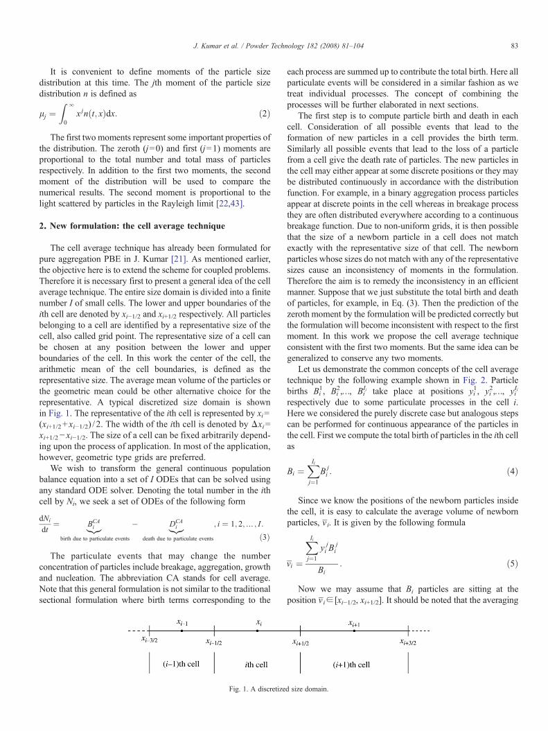
The cell average technique has already been formulated forpure aggregation PBE in J. Kumar [21]. As mentioned earlier,the objective here is to extend the scheme for coupled problems.Therefore it is necessary first to present a general idea of the cellaverage technique. The entire size domain is divided into a finitenumber I of small cells. The lower and upper boundaries of theith cell are denoted by xi−1/2 and xi+1/2 respectively. All particlesbelonging to a cell are identified by a representative size of thecell, also called grid point. The representative size of a cell canbe chosen at any position between the lower and upperboundaries of the cell. In this work the center of the cell, thearithmetic mean of the cell boundaries, is defined as therepresentative size. The average mean volume of the particles orthe geometric mean could be other alternative choice for therepresentative. A typical discretized size domain is shownin Fig. 1. The representative of the ith cell is represented by xi=(xi+1/2+ xi−1/2) / 2. The width of the ith cell is denoted by Δxi=xi+1/2− xi−1/2. The size of a cell can be fixed arbitrarily depend-ing upon the process of application. In most of the application,however, geometric type grids are preferred.

We wish to transform the general continuous populationbalance equation into a set of I ODEs that can be solved usingany standard ODE solver. Denoting the total number in the ithcell by Ni, we seek a set of ODEs of the following form

dNi

dt¼ BCA

i|{z}birth due to particulate events

� DCAi|{z}

death due to particulate events

; i ¼ 1; 2; N ; I :

ð3Þ

The particulate events that may change the numberconcentration of particles include breakage, aggregation, growthand nucleation. The abbreviation CA stands for cell average.Note that this general formulation is not similar to the traditionalsectional formulation where birth terms corresponding to the

Fig. 1. A discretize

each process are summed up to contribute the total birth. Here allparticulate events will be considered in a similar fashion as wetreat individual processes. The concept of combining theprocesses will be further elaborated in next sections.

The first step is to compute particle birth and death in eachcell. Consideration of all possible events that lead to theformation of new particles in a cell provides the birth term.Similarly all possible events that lead to the loss of a particlefrom a cell give the death rate of particles. The new particles inthe cell may either appear at some discrete positions or they maybe distributed continuously in accordance with the distributionfunction. For example, in a binary aggregation process particlesappear at discrete points in the cell whereas in breakage processthey are often distributed everywhere according to a continuousbreakage function. Due to non-uniform grids, it is then possiblethat the size of a newborn particle in a cell does not matchexactly with the representative size of that cell. The newbornparticles whose sizes do not match with any of the representativesizes cause an inconsistency of moments in the formulation.Therefore the aim is to remedy the inconsistency in an efficientmanner. Suppose that we just substitute the total birth and deathof particles, for example, in Eq. (3). Then the prediction of thezeroth moment by the formulation will be predicted correctly butthe formulation will become inconsistent with respect to the firstmoment. In this work we propose the cell average techniqueconsistent with the first two moments. But the same idea can begeneralized to conserve any two moments.

Let us demonstrate the common concepts of the cell averagetechnique by the following example shown in Fig. 2. Particlebirths Bi

1, Bi2,…, Bi

Ii take place at positions yi1, yi

2,…, yiIi

respectively due to some particulate processes in the cell i.Here we considered the purely discrete case but analogous stepscan be performed for continuous appearance of the particles inthe cell. First we compute the total birth of particles in the ith cellas

Bi ¼XIij¼1

B ji : ð4Þ

Since we know the positions of the newborn particles insidethe cell, it is easy to calculate the average volume of newbornparticles, v i. It is given by the following formula

vi ¼

XIij¼1

y ji B

ji

Bi: ð5Þ

Now we may assume that Bi particles are sitting at theposition v i∈ [xi−1/2, xi+1/2]. It should be noted that the averaging

d size domain.

Fig. 2. Appearance of particles in a cell.


process still maintains consistency with the first two moments. Ifthe average volume v i matches with the representative size xithen the total birth Bi can be assigned to the node xi. But this israrely possible and hence the total particle birth Bi has to bereassigned to the neighboring nodes such that the total numberand mass remain conserved. Considering that the averagevolume v iNxi as shown in Fig. 3, the assignment of particlesmust be performed by the following equations

a1ðvi; xiÞ þ a2ðvi; xiþ1Þ ¼ Bi: ð6Þ

and

xia1ðvi; xiÞ þ xiþ1a2ðvi; xiþ1Þ ¼ Bivi: ð7ÞHere a1 (v i, xi) and a2 (v i, xi+1) are the fractions of the birth

Bi to be assigned at xi and xi+1 respectively. Solving the aboveequations we obtain

a1 vi; xið Þ ¼ Bivi � xiþ1

xi � xiþ1; ð8Þ

and

a2 vi; xiþ1ð Þ ¼ Bivi � xixiþ1 � xi

: ð9Þ

It is convenient for further simplifications to define a functionλ as

kFi xð Þ ¼ x� xiF1xi � xiF1

: ð10Þ

The fractions can be expressed in terms of λ as

a1ðvi; xiÞ ¼ Bikþi ðviÞ; ð11Þ

and

a2ðvi; xiþ1Þ ¼ Bik�iþ1ðviÞ: ð12Þ

There are 4 possible birth fractions that may add a birthcontribution at the node xi: two from the neighboring cells andtwo from the ith cell. All possible birth contributions have been

Fig. 3. Average volume of

shown in Fig. 4. Collecting all the birth contributions, the birthterm for the cell average technique is given by

BCAi ¼ Bi�1k

�i ðvi�1ÞHðvi�1 � xi�1Þ þ Bik

�i ðviÞHðxi � viÞ

þ Bikþi ðviÞHðvi � xiÞ þ Biþ1k

þi ðviþ1ÞHðxiþ1 � viþ1Þ:

ð13ÞThe Heaviside step function is a discontinuous function also

known as unit step function and is here defined by

H xð Þ ¼1; xN012; x ¼ 0

0; xb0:

8><>: ð14Þ

Before we summarize the cell average technique it should bementioned here that the continuous number density function n(t,x) can be approximated in terms of Dirac-delta distributions as

nðt; xÞcXIi¼1

Nidðx� xiÞ: ð15Þ

It is due to the fact that all particles in a cell are assumed to beconcentrated at the representative size of the cell. Thisrepresentation of the number density is useful to calculate thediscrete birth and death rates in a cell. We now summarize themain steps of the cell average technique discussed above asfollows:

1. Computation of birth and death rates: The discrete birth anddeath rates can be obtained by substituting a Dirac-deltarepresentation (15) of the density into the continuous form oftotal birth and death rates in a cell. Thereby computations ofBi and Di are performed in the first step.

2. Computation of the volume averages: The second step is tocalculate the average volume of the particles in each cell, i.e.v i. This is a central step of the cell average technique and caneasily be obtained after step 1.

3. Birth modification: The birth modification, crucial point forthe sectional methods, is done according to Eq. (13). Thismodified birth rate Bi

CA is consistent with the first two

all newborn particles.

Fig. 4. Assignment of particles at xi from all possible cells.


moments. Note that there is no need to modify the death termsince particles are just removed from the grid points andtherefore the formulation remains consistent with allmoments due to discrete death. As a result the death termin the cell average formulation Di

CA is equal to Di.4. Solution of the set of ODEs: Substituting the values of Bi

CA

and DiCA into Eq. (3) we obtain a set of ordinary differential

equation. It will be then solved by any higher order ODEsolver. An appropriate solver to solve such equations will berecommended at the end of this section.

A general procedure of the cell average technique has beenexplained above. Further details and implementation of the cellaverage technique for particular and combined processes will bepresented later.

At this point it is important to comment on the conceptualdifference between the fixed pivot and the cell averagetechniques. The basic difference between the two techniques isthe averaging of the volume. The cell average technique firstcollects the total birth of particles in a cell and then distributes itonce to the neighboring nodes depending upon the position ofthe volume average in the cell according to the strategydiscussed above. On the other hand each birth which takesplace in a cell is assigned immediately to the neighboring nodeswith the same strategy by the fixed pivot technique. The anothersubstantial difference as a consequence of the averaging arisesfrom the domain of particles which contributes to birth at a node.The particle domain which may contribute a birth at the node xiis shown in Fig. 5 for both techniques. The cell average coversthe two adjacent cells completely while the fixed pivot techniquetakes the two adjacent cells only partly into consideration.

Up to now we have presented the foundation of the cellaverage technique and illustrated the difference between the twotechniques. We shall now deliberate about the advantages of the

Fig. 5. Particle domain which may c

cell average technique over the fixed pivot technique in general.In order to demonstrate the idea of the cell average and itsimprovements over the fixed pivot technique let us consider asimple example shown in the Fig. 2. As a result of aggregation,breakage or any other event, particle births Bi

1, Bi2, …, Bi

Ii takeplace at the positions yi

1, yi2, …, yi

Ii respectively in the cell i. Asshown in the figure, let us assume that yi

kbxi and yik+1Nxi. In

order to assign them at the nodes xi−1, xi and xi+1 in such a waythat particle number and mass remain conserved, we use thefixed pivot and the cell average strategies. The particle numberassigned at xi by the fixed pivot mechanism is given as

NFPi ¼

Xkj¼1

y ji � xi � 1xi � xi � 1

!B ji þ

XIij¼kþ1

xi þ 1� y ji

xi þ 1� xi

!B ji : ð16Þ

According to the cell average mechanism the total number ofparticles assigned to xi is calculated by either

NCAi ¼ vi � xi � 1

xi � xi � 1

� �XIij¼1

B ji ; if vi V xi; ð17Þ

or

NCAi ¼ xi þ 1� vi

xi þ�xi

� �XIij¼1

B ji ; if viz xi; ð18Þ

depending upon the position of v i in the cell which is defined as

vi ¼

PIij¼1

y ji B

ji

PIij¼1

B ji

: ð19Þ

It is easy to verify that NiCA≥Ni

FP, see Appendix B.1.Equality holds if all particles appear at the same side of the

ontribute a birth at the node xi.


representative xi, Bij=0 for all j≥k+1 or Bi

j=0 for all j≤k.Thus, the number of particles from the ith cell assigned at xi bythe cell average technique is larger than that of the fixed pivottechnique.

From the preceding discussion it is now evident that the cellaverage technique retains more information of the cell, i.e.original particles that belong to the cell, during the assignmentprocess. The fixed pivot technique tends to spread particles, i.e.has more numerical dissipation. In a special case when theaverage of the particles is equal to the representative size nodistribution to neighboring cells takes place by the cell averagetechnique. Assignment of particles to neighboring cells for theconsistency with moments causes numerical diffusion. Since thecell average technique maintains consistency with less particledistribution to neighboring cells, we expect the technique to bemore accurate and less diffusive.

We shall now turn our attention to a suitable ODE solver tosolve the resulting set of ODEs. When integrating the resultantsystem (3) using a standard ODE routine, for example ODE45,ODE15S solvers in MATLAB, this may lead to negativevalues for the number density at large sizes. These negativevalues may lead in the sequel to instabilities of the wholesystem. Therefore, one should take care of the positivity of thesolution by the numerical integration routine. We force thepositivity in our numerical results using an adaptive time stepRunge–Kutta method. The step size adjustment algorithm isbased on embedded Runge–Kutta formulas, originallyinvented by Fehlberg. It uses a fifth-order method with sixfunctions evaluation where another combination of the sixfunctions gives a fourth order method. The difference betweenthe two estimates is used as an estimate of the truncation errorto adjust the step size. A more detailed description of themethod and information about implementation can be foundin [38].

Next we present the derivation of the discrete equations of thecell average technique for several individual and combinedprocesses. Numerical results will be obtained for manyanalytically solvable problems using the cell average techniqueand comparisons will be made with numerical results obtainedby the fixed pivot technique.

2.1. Pure breakage

Now we derive the cell average formulation for the purebreakage. The birth and death terms of the pure breakageequation have already been presented in Eq. (1). The total birthand death rates of particles in the ith cell are calculated byintegrating the birth and death rates from xi−1/2 to xi+1/2 as

Bbreak;i ¼Z xiþ1=2

xi�1=2

Z l

xbðx; ϵÞSðϵÞnðt; ϵÞdϵ dx; ð20Þ

and

Dbreak;i ¼Z xiþ1=2

xi�1=2

SðxÞnðt; xÞdx: ð21Þ

Substituting the Dirac-delta mass representation (15) of thecontinuous number density n (t, x) into the above birth and deathrates, we obtain

Bbreak;i ¼Xk z i

NkðtÞSkZ pik

xi�1=2

bðx; xkÞdx; ð22Þ

and

Dbreak;i ¼ SiNiðtÞ: ð23Þ

Here the limit pki is defined as

pik ¼xi; if k ¼ ixiþ1=2; otherwise:

�ð24Þ

The derivation of the discrete birth and death rates is given inAppendix B.1.1. The total volume flux as a result of breakageinto the cell i is given by

Vbreak;i ¼Z xiþ1=2

xi�1=2

Z l

xxbðx; ϵÞSðϵÞnðt; ϵÞdϵ dx: ð25Þ

Similar to the discrete birth rate we obtain the discrete volumeflux as

Vbreak;i ¼Xk z i

NkðtÞSkZ pik

xi�1=2

xbðx; xkÞdx: ð26Þ

We now compute the volume average of all newbornparticles. Dividing the total volume birth Vbreak,i by the totalnumber birth Bbreak,i, we obtain the volume average v break,i in theith cell as

vbreak;i ¼ Vbreak;i

Bbreak;i: ð27Þ

Now the birth rate for the cell average technique can easily beobtained by substituting the discrete birth rate (22) and thevolume average (27) into Eq. (13). Finally, the resultant set ofODEs takes the following form

dNi

dt¼ Bbreak;i�1k

�i vbreak;i�1

� �H vbreak;i�1 � xi�1

� �þ Bbreak;ik

�i vbreak;i� �

H xi � vbreak;i� �

þ Bbreak;ikþi vbreak;i� �

H vbreak;i � xi� �

þ Bbreak;iþ1kþi vbreak;iþ1

� �H xiþ1 � vbreak;iþ1

� �� SiNi tð Þ:ð28Þ

The set of Eq. (28) is a discrete formulation for solving ageneral breakage problem. The form of breakage and selectionfunction and also the type of grids can be chosen arbitrarily. Theset of Eq. (28) together with an initial condition can be solvedwith any higher order ODE solver to obtain the number ofparticles in a cell Ni.

Fig. 6. Interaction of disperse phase with continuous phase.


2.2. Pure aggregation

In this section we derive the cell average technique for pureaggregation problems. Following J. Kumar [21], the formulationin this case takes the following form

Bagg;i ¼Xjz k

j; kxi�1=2 V ðxjþxkÞ b xiþ1=2

1� 12dj;K

� �bj;kNjNk : ð29Þ

Thus, Bi is the net rate of addition of particles to cell i bycoagulation of particles in lower cells. The net flux of volume Vi

into cell i as a result of these coagulations is therefore given by

Vagg;i ¼Xjz k

j; kxi�1=2 V ðxjþxkÞ b xiþ1=2

1� 12dj;k

� �bj;kNjNk xj þ xk

� �: ð30Þ

Consequently, the average volume of all newborn particles inthe ith cell v i can be evaluated as

vagg;i ¼ Vagg;i

Bagg;i: ð31Þ

Furthermore, the death term is given as

Dagg;i ¼ Ni

XIk¼1

bi;kNk : ð32Þ

Now the final set of discrete equations can be written as

dNi

dt¼ Bagg;i�1k

�i vi�1ð ÞH vi�1 � xi�1ð Þ

þ Bagg;ik�i við ÞH xi � við Þ þ Bagg;ik

þi við ÞH vi � xið Þ

þBagg;iþ1kþi viþ1ð ÞH xiþ1 � viþ1ð Þ � Ni

XIk¼1

bi;kNk : ð33Þ

2.3. Pure growth

As we have mentioned in the previous section that most of themethods for solving growth PBEs suffer from numericaldiffusion. The finite volume schemes are good alternatives tosolve growth PBEs, but they are usually consistent only with asingle moment. Moreover, the extension of the existing finitevolume schemes to arbitrary grids is extremely complicated. Themoving mesh techniques are exceptionally good but they aredifficult to combine with other processes. We have derived atwo-moment consistent discrete formulation for the pureaggregation and pure breakage PBEs and we do expect thesame here. Therefore the aim is to derive a scheme which isconsistent at least with the first two moments, easy to combinewith other processes and can be applied on general grids.

2.4. A new approach for modeling the growth process

In order to accomplish the goal stated above, a completelynew perspective to treat the growth process has been introduced.

The growth of a particle can be treated as adherence of smallnuclei on the particle surface. Traditionally, growth process isdescribed as continuous transfer of mass from the continuousphase to the disperse phase, see Fig. 6(a). Here we consider thisprocess as a combination of two processes. At first, the con-tinuous phase transforms into small nuclei. Then, these nucleiaggregate discretely with the disperse phase. This is shown inFig. 6(b). In this way, the numerical treatment of the growthprocess becomes easier.

Thus, the process can be modeled as aggregation of existingparticles with the imaginary nuclei. The aggregation rate will ofcourse be directly proportional to the growth rate of particles. Likethe aggregation population balance equation, the mathematicalmodel of the growth process then takes the following form

∂nðt; xÞ∂t

¼ b x� x0; x0ð Þn t; x� x0ð Þn t; x0ð Þ � b x; x0ð Þn t; xð Þn t; x0ð Þ:ð34Þ

Here x0N0 is the size of the nuclei. In practice we assume thatthis is a small value. The first term represents the birth at x due toaggregation of nuclei of size x0 with the particles of size x−x0.Similarly the second term describes the death of particles at xdue to aggregation of particles of size xwith the nuclei of size x0.

Unlike the conventional aggregation population balanceequation, Eq. (34) does not contain any integral in the birthand death terms because we have fixed the size of the nuclei andtherefore a single possible event only is responsible to changethe particles at x. Here we assume that the mass m0 (=x0n (t, x0))of the nuclei has a nonzero limit, i.e. m0N0 for x0→0. In thelimit x0→0 this equation leads to the classical form of growthPBE. Let us consider Eq. (34) in the form

∂nðt; xÞ∂t

¼ �x0n t; x0ð Þ bðx; x0Þnðt; xÞ � bðx� x0; x0Þnðt; x� x0Þx0

� �;

ð35Þand take the limit x0→0. This gives

∂nðt; xÞ∂t

¼ �m0∂∂x

b x; x0ð Þn t; xð Þð Þ ¼ � ∂∂x

m0b x; x0ð Þn t; xð Þð Þ:ð36Þ


If we compare this equation directly with the classical PBEfor growth, we get the following relationship between theaggregation kernel β and the mass of the infinitesimally smallnuclei

Gðt; xÞ ¼ m0bðx; x0Þ: ð37Þ

Now the cell average formulation can easily be derived forEq. (34). The numerical discretization of this different form ofthe classical growth PBE will then become easy, consistent withtwo moments and versatile to apply on any type of grids.We shall now formulate the cell average technique for the PBE(34).

2.4.1. Numerical discretizationThe cell average formulation is easy to derive for the new

growth PBE. First we calculate the total birth and death rates inthe cell i as

Bgrowth;i ¼Z xiþ1=2

xi�1=2

bðx� x0; x0Þnðt; x� x0Þnðt; x0Þdx; ð38Þ

and

Dgrowth;i ¼Z xiþ1=2

xi�1=2

bðx; x0Þnðt; xÞnðt; x0Þdx: ð39Þ

We make the assumption that x0 is small enough so that xi+x0bxi+1/2 for all i=1, 2, …, I. This assumption ensures thatparticles just get larger inside the cells and they do not leavetheir cells. Then substituting the number density n (t, x)=∑ j=1

I Njδ(x−xj) into the above birth and death terms gives

Bgrowth;i ¼Z xiþ1=2

xi�1=2

bðx� x0; x0ÞXIj¼1

Njdðx� x0 � xjÞnðt; x0Þdx

¼ bðxi; x0ÞNinðt; x0Þ; ð40Þ

and

Dgrowth;i ¼Z xiþ1=2

xi�1=2

bðx; x0ÞXIj¼1

Njdðx� xjÞnðt; x0Þdx

¼ bðxi; x0ÞNinðt; x0Þ: ð41Þ

The discrete birth and death rate terms are the same in thiscase. Since we assume that the particles are concentrated only atthe pivots, the mass of the particles in the cell will increase andthe total number of particles will remain the same. Similarly thevolume flux into the ith cell is calculated by

Vgrowth;i ¼ bðxi; x0ÞNinðt; x0Þðxi þ x0Þ: ð42ÞIn order to apply the cell average technique, the volume

average will simply be computed by

vi ¼ Vgrowth;i

B¼ xi þ x0: ð43Þ

growth;i

Now the birth has to be modified according to the cell averagestrategy as

BCAgrowth;i ¼ Bgrowth;i�1k

�i ðvi�1ÞHðvi�1 � xi�1Þ

þ Bgrowth;ik�i ðviÞHðxi � viÞ

þ Bgrowth;ikþi ðviÞHðvi � xiÞ

þ Bgrowth;iþ1kþi ðviþ1ÞHðxiþ1 � viþ1Þ: ð44Þ

Since v i≥xi, the modified birth term can be simplified further

BCAgrowth;i ¼ Bgrowth;i�1k

�i ðvi�1Þ þ Bgrowth;ik

þi ðviÞ: ð45Þ

The final formulation of rate of change of number aftersubstituting the expressions of λ and Bgrowth,i in Eq. (45) takesthe following form

dNi

dt¼ b xi�1; x0ð ÞNi�1n t; x0ð Þ vi�1 � xi�1

xi � xi�1

� �

þ b xi; x0ð ÞNin t; x0ð Þ xiþ1 � vixiþ1 � xi

� �� b xi; x0ð ÞNin t; x0ð Þ:

ð46ÞThe aggregation kernel is given by the relationship given in

Eq. (37). The parameter m0 in Eq. (37) can be adjusted equal to1 by fixing a small value of the size of nuclei x0 and choosing n(t, x0)=1/x0. Consequently, the relationship in Eq. (37) changesto G (t, x)=β(x, x0).

In the section of numerical results we will see that formula(46) and the first order upwind discretization produce similarresults. The upwind discretization is a first order finite volumescheme and can be obtained as follows. Direct integration ofpure growth PBE over each cell gives the semi-discreteformulation

dNiðtÞdt

¼ G xi�1=2

� �n t; xi�1=2

� �� G xiþ1=2

� �n t; xiþ1=2

� �; i ¼ 1; 2; N ; I : ð47Þ

Various methods for the numerical solutions of pure growthPBE can be obtained from different choices of the approxima-tion of n (t, xi−1/2) and n (t, xi+1/2) in terms of Ni(t). The easiestapproximation n (t, xi+1/2)≈Ni(t) /Δx gives the first order upwinddifference discretization

dNiðtÞdt

¼ 1Dx

G xi�1=2

� �Ni�1 � G xiþ1=2

� �Ni

� �: ð48Þ

To conclude, the new form of PBE (34) treats the growthprocess as aggregation of existing particle with new small nuclei.The resulting numerical discretization of the growth processbecomes very simple and consistent with first two moments.Additionally, it will be shown later that the new numericalformulation makes it easy to combine the growth process withother processes. Next we will observe that the new discretizationof the growth is a little diffusive but it predicts the first twomoments exactly without any computational difficulties likeappearance of negative values or any other instabilities.


It should be noted that the objective of this work is not toprovide a numerical scheme for pure growth problems but topropose a rather simple and general scheme which can be used tosolve combined processes effectively. Several finite volume andfinite element schemes can be found in the literature which maybe used to solve the growth PBEs but all of them either haveproblems with consistency of moments or they are not easy tocombine with other particulate processes. In the next section wewill show that the coupling of the growth process with otherparticulate processes using the cell average technique becomestrivial and considerably better results for combined processescan be obtained without much extra computational effort.

2.5. Simultaneous aggregation and breakage

This subsection is devoted to the numerical treatment ofcombined aggregation and breakage processes. When bothaggregation and breakage processes take place together, thediscrete birth and death rates for combined processes in most ofthe numerical schemes are generally considered by algebraicallysumming the individual birth and death rates. In other words,conventionally the easiest way to couple the two processes isto just add the corresponding discretizations in the followingway.

dNi

dt¼ BCA

agg;i þ BCAbreak;i � Dagg;i � Dbreak;i; ð49Þ

This formulation is of course consistent with the first twomoments if this holds for breakage and aggregation separately.In order to couple the two discretizations more efficiently wetake advantage of the cell average technique. The accuracy canfurther be improved by using the idea of cell average for thecombined problem simply by considering the total birth anddeath rates from combined processes. Thereby, we shall treatboth processes together in a similar way as we have treated theindividual processes. First we collect all the newborn particles ina cell independently of the events that make them appear in thecell. In our case here the events are aggregation and breakageprocesses. Then we take the volume average of all newbornparticles in the cell. The remaining steps are the same we usedfor the individual processes of aggregation or breakage.Mathematically, we construct the discrete formulation for thecoupled problem as

dNi

dt¼ BCA

aggþbreak;i � Daggþbreak;i: ð50Þ

Here the terms Bagg+break,iCA and Dagg+break,i represent the birth

and death rates of particles in the cell i due to aggregation andbreakage respectively. The total birth and death rates in ith cell isgiven by

Baggþbreak;i ¼ Bagg;i þ Bbreak;i; ð51Þand

D ¼ D þ D : ð52Þ
aggþbreak;i agg;i break;i
Now the birth rate Bagg+break,i has to be modified to make theformulation consistent with respect to the first two moments.Thus, the modified birth term or the cell average birth term willbe then computed as

BCAaggþbreak;i ¼ Baggþbreak;i�1k


þ Baggþbreak;ik�i ðviÞHðxi � viÞ

þ Baggþbreak;ikþi ðviÞHðvi � xiÞ

þ Baggþbreak;iþ1kþi ðviþ1ÞHðxiþ1 � viþ1Þ: ð53Þ

The truly new ingredient is that the average value v i will becomputed as

vi ¼ Vagg;i þ Vbreak;i

Bagg;i þ Bbreak;i: ð54Þ

The terms Bagg,i, Bbreak,i, Dagg,i, Dbreak,i, Vagg,i, Vbreak,i andalso the λi are the same as given in the previous sections. Nextwe will test the coupled formulation on two test problems. Themodified birth term (53) and the death term (52) can besubstituted in Eq. (50) to get the final formulation. We will seethat the new way of coupling is not only more accurate but alsocomputationally less expensive. This is evident since in the lattercase we are distributing particles once while in the conventionalapproach particles are distributed twice; once due to aggregationand then due to breakage.

2.6. Simultaneous aggregation and nucleation

As in the previous section we have just considered that theparticles are appearing in cells independently of the event thatmake them appear and presented a cell average formulation forcombined aggregation and breakage processes. A similarapproach has to be applied here for the case of simultaneousaggregation and nucleation. The process of nucleation may beintroduced into the modeling in two ways. A common approachis via a boundary condition at particle size 0 if the nucleation ismono-disperse. Here we want to consider the alternative of asource located near particle size 0. In a continuum theory bothare valid approaches.

Before we proceed to the final form of the cell averagetechnique, we want to comment on the conventional coupling ofthese processes. Let us discuss the case of discretization ofKumar and Ramkrishna [23] for simultaneous aggregation andnucleation, they considered

dNi

dt¼ discretization due to aggregationþ

Z xiþ1=2

xi�1=2

Bnuc t; xð Þdx:

ð55ÞNote that in the above formulation we may gain or loose

mass if the nucleation does not take place exactly at therepresentative sizes xi. It is possible that the particles couldagain be distributed to neighboring cells for the consistency ofmoments in the fixed pivot technique. We are not interestedhere to explore more about this issue. We now present how todeal with these problems with the cell average techniques


efficiently. Similar to previous section, we wish to have thefollowing discretization

dNi

dt¼ BCA

aggþnuc;i � Dagg;i: ð56Þ

Since nucleation is the birth of the particles, there is nonucleation term to be considered in the death term. An analogouscontribution to the death term would come if we consideredharvesting of certain particle sizes. The numerical treatmentwould be analogous. Now the birth by nucleation and aggregationcan be described as follows

BCAaggþnuc;i ¼ Baggþnuc;i�1k


þ Baggþnuc;ik�i ðviÞHðxi � viÞ

þ Baggþnuc;ikþi ðviÞHðvi � xiÞ

þ Baggþnuc;iþ1kþi ðviþ1ÞHðxiþ1 � viþ1Þ: ð57Þ

where

Baggþnuc;i ¼ Bagg;i þZ xiþ1=2

xi�1=2

Bnucðt; xÞdx: ð58Þ

The average values are computed as

vi ¼Vagg;i þ

Z xiþ1=2

xi�1=2

xBnucðt; xÞdx

Bagg;i þZ xiþ1=2

xi�1=2


All other notations appearing in the formulation are alreadydefined in previous sections. So treating nucleation andaggregation as particle birth in cells in a similar fashion wehave gained the consistency with the first two moments. It shouldbe noted that if the nucleation is mono-disperse, usually theappearance of smallest particle, and the smallest representative ischosen such that it matches exactly with the size of the mono-disperse particles, then the above formulation can be rewritten as

dN1

dt¼ BCA

agg;1 � Dagg;1 þ Bnuc t; x1ð Þ;and

dNi

dt¼ BCA

agg;i � Dagg;i; i ¼ 2; 3; N ; I : ð60Þ

The formulation (56) may be used for a general poly-dispersenucleation and formulation (60), a particular case of (56), is usedfor mono-disperse nucleation.

2.7. Simultaneous growth and aggregation

This section is devoted to the numerical treatment of thesimultaneous growth and aggregation processes. As we have seenthat the cell average technique can be applied to solve a puregrowth problem by the application of a different form of growthPBE. Similar to other combined processes, in this case we like tohave the following form of the cell average formulation

dNi

dt¼ BCA

aggþgrowth;i � Daggþgrowth;i: ð61Þ

Here the birth and death terms in above equation aregiven as

BCAaggþgrowth;i ¼ Baggþgrowth;i�1k


þ Baggþgrowth;ik�i ðviÞHðxi � viÞ

þ Baggþgrowth;ikþi ðviÞHðvi � xiÞ

þ Baggþgrowth;iþ1kþi ðviþ1ÞHðxiþ1 � viþ1Þ; ð62Þ

and

Daggþgrowth;i ¼ Dagg;i þ Dgrowth;i; ð63Þwhere

Baggþgrowth;i ¼ Bagg;i þ Bgrowth;i: ð64ÞThe volume average of particles appearing due to growth and

aggregation in the cell i is calculated as

vi ¼ Vagg;i þ Vgrowth;i

Bagg;i þ Bgrowth;i: ð65Þ

The discrete Eq. (61) has been used in our simulations tocalculate the evolution of particle size distribution and itsmoments.

For comparison we describe an alternative by which the twoprocesses can be coupled in a different manner which is moreaccurate but more expensive. For the simultaneous aggregationand growth, one may use cell average technique for theaggregation and a Lagrangian approach for the growth to obtaina better accuracy of the numerical results. Finally, we solve thefollowing set of ordinary differential equations for thesimultaneous growth and aggregation

dNi

dt¼ BCA

agg;i � Dagg;i; ð66Þ

together with

dxidt

¼ G xið Þ; ð67Þ

and

dxiþ1=2

dt¼ G xiþ1=2

� �: ð68Þ

The first equation is for the rate of change of particle due toaggregation while the last two equations describe the motion ofthe representatives and boundaries respectively. A similarapproach can be used to couple growth process with otherprocesses like breakage or simultaneous breakage and aggrega-tion. In this work we only presented numerical results for the cellaverage technique where analytical solutions are easily availablebut it can be formulated in a similar fashion for other com-binations of processes.

2.8. Simultaneous growth and nucleation

Similar to the case of simultaneous aggregation andnucleation, see Section 2.6, it is easy to couple the growth and

1 It is convenient to express the extent of aggregation by a dimensionlessform of zeroth moment, also known as degree of aggregation. It is defined as1−μ(t) /μ(0).


nucleation processes. The cell average formulation in this case isgiven as

dNi

dt¼ BCA

growthþnuc;i � Dgrowth;i: ð69Þ

Now the birth by nucleation and growth can be described asfollows

BCAgrowthþnuc;i ¼ Bgrowthþnuc;i�1k


þ Bgrowthþnuc;ik�i ðviÞHðxi � viÞ

þ Bgrowthþnuc;ikþi ðviÞHðvi � xiÞ

þ Bgrowthþnuc;iþ1kþi ðviþ1ÞHðxiþ1 � viþ1Þ; ð70Þ

where

Bgrowthþnuc;i ¼ Bgrowth;i þZ xiþ1=2

xi�1=2


The average values are computed as

vi ¼Vgrowth;i þ

Z xiþ1=2

xi�1=2

xBnucðt; xÞdx

Bgrowth;i þZ xiþ1=2

xi�1=2


To conclude, we have presented the cell average formulationfor some cases of coupling the two selected processes. But theidea remains the same to couple any number of arbitraryprocesses. In the next section we proceed to compare thenumerical results with the analytical solutions in different casesconsidered before.

3. Numerical results

In this section, the performance of the cell average techniqueis evaluated by a direct comparison of the PSD and its momentscalculated by the fixed pivot technique as well as with theanalytical solutions. Several pure and combined processes thatcan be solved analytically have been considered in ourcomparisons. The analytical solutions in each case togetherwith initial condition have been provided in Appendix A.

The comparison between numerical and analytical results iscarried out by means of average number density. Since the totalnumber of particles in each cell is obtained from the numericaltechniques, it is fair to compare the average number density. Itcan be calculated in the following way

nnumi ¼ Ni

Dxi; ð73Þ

where Δxi=xi+1/2−xi−1/2. Similarly, from the analytical resultswe get

nanai ¼ 1Dxi

Z xiþ1=2

xi�1=2

n t; xð Þdx: ð74Þ

These densities have been plotted at grid points. This criterionof comparison is used in the entire work. The integration

appearing in the analytical average density is computed eitheranalytically if possible otherwise numerically by a low orderintegration routine. It should be mentioned that in all followingcomputations, the volume domain is discretized geometricallyinto small cells by the rule xi+1/2=2

1/qxi−1/2. The parameter qadjusts the coarseness of the mesh.

3.1. Pure breakage

Let us first assess the accuracy of the scheme for purebreakage. Here we have considered only two test cases of binarybreakage with linear and quadratic selection functions, seeAppendix A.1. Fig. 7 compares the average number densitiesobtained by the two methods with the analytical one for both testcases. The figures have been plotted on a semi-log scale, log in xaxis and linear in y axis, to show the performance of the cellaverage technique predicting the particle distribution at smallsize range. Since particles flow towards the lower size range inthe breakage process, it is important to check the performance ofthe scheme to predict these small particles. In this simulation thenumber of geometric grid points is taken to be 30. As can beseen, the PSD obtained by the cell average technique is inexcellent agreement with the analytical solution even for a verycoarse grid. On the other hand the fixed pivot technique over-predicts the numerical results. Here we present only two testcases. Other comparisons as well as mathematical analysis willbe presented somewhere else.

Based on the above results, one can conclude that thenumerically calculated PSDs by the two methods deviate fromeach other significantly. The numerical results calculated fromthe cell average technique on a coarse geometric grid are veryaccurate. On the other hand, an over-prediction in the PSD atlower volumes has been observed in the fixed pivot technique.The computation time taken by the cell average technique isslightly more than for the fixed pivot technique.

3.2. Pure aggregation

The performance of the scheme for pure aggregationproblems has already been published in J. Kumar et al. [21]and Kostoglou [16]. Therefore, for completion, we present hereonly one test case taken from J. Kumar et al. [21].

The analytical and numerical results for the mono-disperseinitial condition with the sum kernel have been shown in Fig. 8.The analytical solutions of this test case are given in AppendixA.2. The computation in this case is performed at 0.80° ofaggregation.1 Fig. 8 clearly shows the improvement of the over-prediction in PSD at large particle sizes by the cell averagetechnique over the fixed pivot technique. Fig. 8(a) includes acomparison of the analytical and numerical solutions for thevariation of the second moments for the size dependent sumkernel. Once again, the agreement is very good by the cell

Fig. 7. A comparison of particle size distributions on semi-log scale for mono-disperse initial condition.

Fig. 8. A comparison of numerical with analytical results for mono-disperseinitial condition and sum kernel, q=1 and Iagg=0.80.


average technique and the same diverging behavior is observedby the fixed pivot technique. Comparison of size distribution ismade in Fig. 8(b). As for the case of size-independentaggregation, the prediction is poor at large particle sizes by thefixed pivot technique. Once more the degree of fit is very high inthe case of the cell average technique.

3.3. Pure growth

We have considered two test cases to access the ability of thescheme to handle pure growth problems. In the first test case wetake exponentially distributed particle size distribution

n 0; xð Þ ¼ N0

x0exp �x=x0ð Þ; ð75Þ

with a linear growth rate G(x)=x. The second test case considersthe step function as an initial condition with a constant growthrate. The analytical results for the number density and differentmoments are given in Appendix A.3.

Fig. 9(a) shows numerical results for the first two momentscalculated using the cell average technique and the first order

upwind discretization. Since the cell average formulation isconsistent with the first two moments, the prediction of the firsttwo moments using the cell average technique is exact. On theother hand the upwind discretization shows a diverging behaviorof the first moment. The prediction of the zeroth moment by theupwind discretization is excellent due to automatic conservingproperty of the upwind discretization. The corresponding particlesize distribution at the final time is plotted in Fig. 10(b). Theprediction of the particle size distribution by the two techniquesis quite similar. A small over-prediction of the results by the cellaverage technique has been observed at the small as well as atlarge volumes. The number density at the small volumes by theupwind discretization is pretty good whereas it is consistentlyover-predicting at the large volumes.

The numerical results for the second test case have beenpresented in Fig. 10. For the constant growth rate numericalresults obtained using both techniques are quite similar.Nevertheless, once more, the prediction of the first moment bythe upwind discretization, shown in Fig. 10(a), is slightly over-estimated. Whereby both the moments calculated using the cellaverage technique are exactly matching with the analyticalresults. Fig. 10(b) shows that the numerical results for the

Fig. 9. A comparison analytical and numerical results for pure growth usingexponentially distributed initial particle size distribution and linear growth rate,grid points 130.

Fig. 10. A comparison analytical and numerical results for pure growth usingstep function as initial particle size distribution and constant growth rate, gridpoints 95.


particle size distribution are highly diffusive. It is due to the factthat we have chosen a discontinuous initial condition. Most ofthe numerical schemes smear out near discontinuities and highergradients. Very fine grids near discontinuities are often requiredto capture the complete details of the distribution.

As we have seen the numerical results of the particle sizedistribution for pure growth problems by the cell average tech-nique as well as by the upwind discretization are not veryaccurate. A better accuracy in this case can be obtained bymaking the formulation consistent with the first three moments,see for details J. Kumar [20].

3.4. Combined aggregation and breakage

We compared the fixed pivot technique [22] and the cellaverage technique with analytically solvable problems proposedby Patil and Andrews [35]. Later these solutions were slightlysimplified by Lage [24] to the form we use here. A list ofanalytical solutions used here has been included in Appendix A.4.They considered a special case of simultaneous aggregation andbreakage where the number of particles stays constant witha uniform binary breakage b(x, y)=2/y, linear selection function

S(x)=S0x and constant aggregation kernel β(x, y)=β0. They usedthe following two types of initial conditions

n 0; xð Þ ¼ N0 2N0

x0

2x exp �2

N0

x0x

� �; ð76Þ

and

n 0; xð Þ ¼ N0N0

x0exp �N0

x0x

� �: ð77Þ

Note that next to conservation of mass these problems havethe special properties that the processes of aggregation andbreakage balance to conserve total number also. Data (77) are asteady state solution.

We have discretized the volume domain geometrically usingthe rule xi+1/2=2xi−1/2. Fig. 11(a) and (b) shows a comparison ofthe particle size distributions for the initial condition (76) at timet=0.4 and t=6 respectively. As can be seen from the figures, thecell average technique is able to approximate the PSD to a veryhigh degree of accuracy. On the other hand a small over-prediction is observed at the smaller volumes by the fixed pivottechnique.

Fig. 11. A comparison of particle size distributions for binary breakage andaggregation with initial condition (76), grid points 38.


Let us now consider the steady state data (77). The results forthis case are presented in Fig. 12. The prediction by the cellaverage technique is again excellent in this case while a similarover-prediction by the fixed pivot technique can be observed.Actually this over-prediction grows with time, i.e. the fixed pivottechnique is not stable with respect to steady states. Furthermore,the same numerical results for both the initial conditions at thefinal time have been plotted on a log–log scale in Fig. 13. Onceagain we can see here that the prediction of PSD by the cellaverage technique is superior to the prediction with the fixedpivot technique.

We shall now demonstrate the difference between conven-tional coupling (49) of the cell average technique appliedseparately to aggregation and breakage and the new cell averagecoupling (50). Note that we are not considering the fixed pivottechnique in this comparison. Since the numerical results areindistinguishable from the analytical results for the steady stateinitial condition (77), we have only compared the numericalresults for the unsteady initial condition (76). The numericalresults have been plotted in Fig. 14. The L1 error

2 between the

2 L1 error=∑i|Niana−Ni

num|.

numerical and analytical results of PSD has also been reported inthe figure. Due to the simplicity of the problem, uniform binarybreakage, the difference between the two types of coupling is notso significant. Nevertheless, the cell average type coupling (50)gives better results which can be observed at the steep part of thePSD as well as from the L1 error. Another difference has beenobserved in computational time. The cell average type coupling(50) takes about 38 s CPU time while conventional coupling (49)takes 52 s CPU time on a Pentium-4 machine with 1.5 GHz and512 MB RAM.

To summarize, the cell average technique provides highlyaccurate results already on a very coarse grid. The accuracy canof course be further increased by making the grid finer. The cellaverage technique with the new coupling makes the techniqueeven more useful for combined aggregation and breakage bybeing not only more accurate but also computationally lessexpensive.

3.5. Combined aggregation and nucleation

We have tested the formulation for simultaneous nucleationand aggregation. A simple case of zero initial population withconstant aggregation kernel and mono-disperse nucleation is

Fig. 12. A comparison of particle size distributions for binary breakage andaggregation with initial condition (77), grid points 38.

Fig. 13. A comparison of particle size distributions at t=6 for binary breakageand aggregation plotted on log–log scale, grid points 38.


considered. Such systems with zero initial population usuallylead to oscillations in the particle size distribution. But we willsee by numerical results that the cell average technique iscompletely free of oscillations. Analytical solutions for the firsttwo moments of this problem reported by Alexopoulos and

Fig. 14. A comparison of particle size distributions for binary breakage andaggregation showing the difference between conventional coupling and cellaverage coupling, grid points 38.

Kiparissides [2] have been included in Appendix A.5.Formulation (60) is used for the computation in this particularcase.

In Fig. 15(a), a comparison is made between the exactsolutions of the first two moments and the numerical solutioncalculated using the cell average formulation (60) for the caseβ0=1 and Bnuc(t, x1)=1. The volume domain is discretizedgeometrically into 30 cells starting with 10−6. As can be seenfrom the figure the numerical results are in excellent agreementwith the analytical results. It should be mentioned that, after acertain time, the total number of particles in the system isinvariant. A dynamic equilibrium with respect to the totalnumber has been reached at that time. In other words the particlenucleation rate becomes equal to the total particle aggregationrate. On the other hand, the total mass of the particles which isproportional to the first moment increases linearly with respectto the process time. Unfortunately an analytical solution for thecomplete PSD is not easily available, only numerical results atdifferent times have been depicted in Fig. 15(b). A quitecomplicated but systematic behavior of the results has beenobserved. Clearly the particle size distribution is free fromoscillations.

Fig. 15. Numerical results for simultaneous nucleation and aggregation, gridpoints 30.


3.6. Combined growth and aggregation

In order to demonstrate the effectiveness of the cell averagetechnique we have applied it to two test problems with a lineargrowth rate G(x)=G0x. The constant kernel β(x, y)=β0 and thesum kernel β(x, y)=β0(x+y) for aggregation are used in the firstand second test problems respectively. An exponentiallydecreasing particle size distribution has been used as initialcondition. The initial condition and analytical solutions for theparticle size distribution as well as its moments are given inAppendix A.6. The particle volume domain was partitioned into60 non-homogeneous cells with the rule xi+1/2=2

1/qxi−1/2.Numerical results for the first test problems have been plotted

in Fig. 16. The variation of the first two moments with time ispresented in Fig. 16(a). The numerical and analytical solutionsfor moments are in excellent agreement. On the other handnumerical results for the particle size distribution at final time,shown in Fig. 16(b), are slightly over-estimated. A betteraccuracy, of course, can be achieved by refining the grids.

A similar computation has been performed for the second testcase of size-dependent aggregation kernel. Once more thenumerical solution of the first two moments overlaps theanalytical solutions excellently, see Fig. 17(a). The number

Fig. 16. Simultaneous growth and aggregation using the cell average technique,β (x, y)=β0 and G (x)=G0x, grid points 65.

Fig. 17. Simultaneous growth and aggregation using the cell average technique,β (x, y)=β0(x+y) and G (x)=G0x, grid points 65.

density distribution at final time together with the initialcondition is plotted in Fig. 17(b). As can be seen from thefigure a very good agreement between the analytical andnumerical solutions has been obtained.

We can conclude that the cell average technique can be usedfor coupled processes effectively. The coupling of growthprocesses with aggregation and breakage has been a big issue inareas related to particulate systems. Different authors proposeddifferent coupling techniques but all of them either arecomplicated [23], less accurate and unstable [13] or applicableto limited problems [14,37]. The application of the cell averagetechnique to combined different processes is easy as well asconsistent and produces comparatively good results.

As mentioned before growth processes can be coupledwith other processes by computing growth using Lagrangianapproach and aggregation or breakage using the cell averagetechnique. In this way numerical diffusion by the growth cansignificantly be reduced and considerably better results can beobtained. In order to illustrate this coupling we have consideredthe same test cases as before. Since the prediction of the first twomoments in this case is similar to the previous case, we omittedthem to present here. Only the particle size distributionscorresponding to Figs. 16(b) and 17(b) have been plotted in

Fig. 19. A comparison of particle size distributions with no particles initiallypresent in the system, grid points 120.


Fig. 18(a) and (b). Clearly, it can be seen from the figures that theaccuracy of the numerical results has been improved in bothcases.

3.7. Combined growth and nucleation

Nucleation with no particles initially present is difficult tosimulate. The analytical solution together with the initialcondition is included in Appendix A.7. The volume domainhas been partitioned into 100 geometrically spaced cells. Acomparison between the analytical and numerical solution isshown in Fig. 19. As can be seen from the figure the numericalresults are slightly diffusive. Very fine grids are needed tocapture the details near discontinuity.

As we have seen in previous sections the coupling of growthwith other processes using a Lagrangian approach producesexcellent results. An attempt in this direction has been made byKumar and Ramkrishna [23]. Numerical treatment of simulta-neous growth and nucleation using the Lagrangian approach isnot trivial because smallest representative sizes together withtheir boundaries will move and there may not be a cell to placesubsequently formed nuclei. This definitely forces us to addmore cells as the PSD moves to the right and therefore it leads to

Fig. 18. Simultaneous growth and aggregation using the cell average techniquefor aggregation and Lagrangian approach for growth, grid points 65.

serious difficulties in numerics. The formulation of Kumar andRamkrishna [23] is inconsistent with the mass of the particlesdue to nucleation. It was later improved by Spicer et al. [45] byconsidering the effect of the mass of new formed nuclei on themovement of cell representatives.

3.8. From the cell average to the fixed pivot technique

Now we shall divert our attention to the concept of choosingrepresentative sizes and find out some similarities of the fixedpivot and cell average schemes. In practice, the representativesize of a cell may be chosen arbitrarily. The center of the cell, aneasy choice, is a common choice for the representative size. Onthe basis of the position of the representative sizes we have thefollowing lemma which tells us about the similarity of twotechniques.

Lemma 3.1. If we choose the representative sizes xi as aboundary of cells then both the cell average and fixed pivotschemes become the same, i.e.

dNi

dt

� �CA

¼ dNi

dt

� �FP

if xi ¼ xiF1=2: ð78Þ

Proof. Consider some particles n1, n2,…, nm of respective sizesx1, x2,…, xm appear in the ith cell due to aggregation, breakageor any other event. Let us suppose that the representative size xiof this cell lies at the left boundary xi−1/2. In order to makeparticles appearance consistent with their number and mass,only a fraction of them has to be assigned at xi. We calculate thefraction assigned at xi using the cell average and the fixed pivottechniques. It is evident that the particles have to be distributedbetween xi and xi+1 according to both techniques. The assignedfraction of particles at xi according to the fixed pivot techniqueis given as

aFP ¼ xiþ1 � x1xiþ1 � xi

� �n1 þ xiþ1 � x2

xiþ1 � xi

� �n2 þ N þ xiþ1 � xm

xiþ1 � xi

� �nm:

ð79Þ


According to the cell average technique, the fraction is givenby

aCA ¼ xi þ 1� v1xi þ 1� xi

� �n1 þ n2 þ N þ nnð Þ; ð80Þ

where the average value v i is computed as

vi ¼ x1n1 þ x2n2 þ N þ xmnmn1 þ n2 þ N þ nm

: ð81Þ

Clearly substitution of the average v i from Eq. (81) intoEq. (80) gives the required result (79), i.e. aFP=aCA. Tosummarize, if the representative size of a cell lies at one of theboundaries then taking average and assigning a fraction of allparticles to the neighboring representatives is the same asassigning particles of each size separately without takingaverage of them. □

4. Conclusions

This work presents the extension of a numerical scheme, thecell average technique that we introduced in J. Kumar [21], forsolving population balance equations. The technique is based onthe fixed pivot technique developed by Kumar and Ramkrishna[22]. The cell average technique follows a two step strategy, oneto calculate average size of the newborn particles in a class andthe other to assign them to neighboring nodes such that theproperties of interest (moments) are exactly preserved. A com-parison of the numerical results obtained by the fixed pivot andcell average techniques with the analytical results indicates thatthe cell average technique improves the over-prediction of thenumber density distribution.

The cell average technique proposed in this work allows theconvenience of using regular (linear, geometric or equal size) andirregular meshes. Furthermore, the cell average scheme isconsistent with the zeroth and first moments, the same procedurecan be used to provide consistency with any two or more than twomoments. Consistency with more than two moments can beachieved by distributing particles to more grid points. Thenumerical results have shown the ability of the cell averagetechnique to predict very well the time evolution of the secondmoment as well as the complete particle size distribution. Animportant attribute of a numerical scheme, the computationaltime, has been investigated for numerous problems. It has beenfound that the computation time taken by the cell averagetechnique is comparable to that taken by the fixed pivot technique.Moreover, for several aggregation problems it was even less thanthe computation time taken by the fixed pivot technique.

A new approach for solving growth population balanceequations is presented. The growth process has been treated asaggregation of existing particles in the disperse phase with someimaginary nuclei appearing from the continuous phase. Thus, thegrowth population balance equation is converted to theaggregation population balance equation. The aggregation rateis expressed in terms of the growth rate. Consequently, itbecomes a trivial task to apply the cell average technique to thetransformed aggregation population balance equation. However,

numerical results of the particle size distribution turn out to bevery diffusive. Nonetheless, the cell average formulation pre-dicts the first two moments extremely accurately without anycomputational difficulties.

Furthermore, a new concept for the coupling of differentprocesses has been introduced. All processes including growthand nucleation have been solved using the cell average techniqueby treating them uniformly. It has been demonstrated that thenew approach of coupling is not only more accurate but alsocomputationally less expensive. This is achieved by collectingall newborn particles in a cell independently of the events(aggregation, breakage, growth and nucleation processes) thatmake them appear in the cell. Then a similar treatment like thecell average technique provides to individual processes is given.A substantial success of this coupling is observed for combinedprocesses where growth is present because the coupling ofgrowth with other processes has been a challenging task. Thenew approach of coupling makes the numerical discretizationvery simple and more accurate.

Nomenclature
a1, a2,a3, a4
Fraction of particles
–
b
Breakage function m−3
B
Birth rate m−6
s−13

B
Binary breakage function m−
s−1

C
Constant –6
D
Death rate m−
s−1

E
Error – Gj Growth rate along internal
coordinate j
[ij]/s
H
Heaviside function – I Total number of cells – Iagg Degree of aggregation – K Constant –
6

n
Number density function m−3
N
Number m−3
N0
Initial number of particles m−
pki
Limit of integral defined by
the function (24)
m3
q
Discretization parameter –1
Q
Flow rate m3 s−
r
Ratio xi+1/xi –1
S
Selection function s−
t
Time s Ta Dimensionless time
for aggregation
−
Tg
Dimensionless time for growth − Ts Dimensionless time simultaneous
processes
−
u, v, x
Volume of particles m3
v
Average volume m3
V
System volume m3
v0, x0
Initial mean volume m3


Greek symbols
α Integer – β One-dimensional aggregation kernel m3 s−1
1

β
Multidimensional dimensionalaggregation kernel
m3 s−

δ (x)
Dirac-delta distribution – δij Kronecker delta – Δx Size of a cell – ϵ Global truncation error – η Particle distribution function – λ Fractions – Λ Discretized domain – μr The rth moment m3r
m− 3

μ
Logarithmic norm – ν Parameter in Gaussian-like
distribution
–
σ
Spatial truncation error – τ Age of particles s ф Limiter function – ω Constant –
Subscriptsagg Aggregationbreak Breakagei, j Indexin Inletnuc Nucleationout Outlet

Superscriptsˇ Constant values¯ Mean or average valuesˆ Numerical approximationsana Analyticalmod Modifiednum Numerical

AcronymsCA Cell averageDPBE Discretized population balance equationFP Fixed pivotGA Generalized approximationGSD Granule size distributionMOL Method of lineODE Ordinary differential equationPBE Population balance equationPPD Particle property distributionPSD Particle size distribution

Acknowledgements

This work was supported by the Graduiertenkolleg-828,‘Micro–Macro-Interactions in Structured Media and ParticlesSystems’, Otto-von-Guericke-Universität Magdeburg. Theauthors gratefully thank for funding through this PhD program.

Appendix A. Analytical solutions

A.1. Pure breakage

Ziff and McGrady [51] provided the analytical solutions forvarious initial conditions and different breakage and selectionfunctions. For mono-disperse initial condition n (0, x)=δ (x−L),we summarize here only in two different cases.

Case 1 The analytical solution for the case S(x)=x and β(x, y)=2/y, is given as

nðt; xÞ ¼ expð�txÞðdðx� LÞ þ ½2t þ t2ðL� xÞ�hðL� xÞÞ:ð82Þ

Case 2 For the case S (x)=x2 and β (x, y)=2/y, the solutiontakes the following form

nðt; xÞ ¼ expð�tx2Þ½dðx� LÞ þ 2tLhðL� xÞ�: ð83Þ

Here the function θ is the step function defined as

hðx� LÞ ¼ 1; xbL0; otherwise:

�ð84Þ

A.2. Pure aggregation

The analytical solution for mono-disperse initial conditioncan be found in Aldous [1]. For the sum β (x, y)=x+y kernel, theanalytical number density is given

nðt; xÞ ¼ expð�tÞBð1� expð�tÞ; xÞ; with 0V t bl; ð85ÞHere the function B is defined as

Bðk; xÞ ¼ ðkxÞx�1expð�kxÞ=x!; x ¼ 1; 2; N ; 0V kV1: ð86Þ

A.3. Pure growth

A.3.1. Constant growth rateMoments: The rate of change of the zeroth and first moment

is given by

l0ðtÞ ¼ l0ð0Þ: ð87Þand

l1ðtÞ ¼ l1ð0Þ þ G0l0ð0Þt: ð88ÞNumber density: The growth rate is constant, so all points on

the solution profile will move at the same speed G(x)=G0. If n0(x) is the initial solution, then the time evolution of numberdensity is given by

nðt; xÞ ¼ n0ðx� G0tÞ: ð89Þ

A.3.2. Linear growth rateMoments: as we have seen that the rate of change of the

zeroth moment is always zero independently of growth rate.


Therefore the zeroth moment remains constant during thegrowth process i.e. μ0(t)=μ0(0). The rate of change of the firstmoment in this case is calculated by

l1ðtÞ ¼ l1ð0ÞexpðG0tÞ: ð90ÞNumber density: For linear growth rate, G(x)=G0x, Kumar

and Ramkrishna [23] have provided the analytical solution forpure growth PBE

nðt; xÞ ¼ n0ðx expð�G0tÞÞexpð�G0tÞ; ð91Þ

where n0(x) is the initial particle size distribution.

A.4. Simultaneous aggregation and breakage

Patil et al. [35] provided an analytical solution for the PBEwith simultaneous breakage and coalescence for a special casewhere the total number of particles is constant. They consideredthe following continuous PBE

∂nðv; tÞ∂t

¼ 12

Z v

0b v� u; uð Þn v� u; tð Þn u; tð Þdu

� n v; tð ÞZ l

0b v; uð Þn u; tð Þdu

þ 2Z l

vS uð Þn u; tð Þb v; uð Þdu� S vð Þn v; tð Þ; ð92Þ

with the constraints

nðv; 0Þz 0;0Vbðu; vÞ ¼ bðv; uÞ;Z w

0bðv;wÞdv ¼ 1;Z w

02vbðv;wÞdv ¼ w:

Kernels are

bðu; vÞ ¼ b0;SðvÞ ¼ S0v;

b v; uð Þ ¼ 1u:

Analytical solutions are obtained for the following two initialconditions

n v; 0ð Þ ¼ N 0ð ÞNð0Þl1

exp �Nð0Þl1

v

� �; ð93Þ

and

n v; 0ð Þ ¼ N 0ð Þ 2Nð0Þl1

� �2

v exp �2Nð0Þl1

v

� �; ð94Þ

where N (t) is the total number of particles and μ1= ∫0∞ vn (v, t)dv is the first moment of the distribution. It can also be provedthat the total number is constant by choosing the values of the

problem parameters to satisfyffiffiffiffiffiffiffiffiffiffiffiffiffiffiffiffiffiffiffi2S0l1=b0

p ¼ Nð0Þ. Theyintroduced the following dimensionless variables

U Tsð Þ ¼ NðtÞNð0Þ ; g ¼ vNð0Þ

l1; ð95Þ

Ts ¼ N 0ð Þb0t; and / g; Tsð Þ ¼ nðv; tÞl1½Nð0Þ�2 : ð96Þ

Now, Eq. (92) can be written in dimensionless form as

∂/∂Ts

¼ 12

Z g

0/ g� x; Tsð Þ/ x; Tsð Þdx� / g; Tsð ÞU Tsð Þ

þ U lð Þ�2Z l

g/ x; Tsð Þdx� g

2U lð Þ�2/ g; Tsð Þ;h

ð97Þ

with the initial condition

/ðg; 0Þ ¼ expð�gÞ or /ðg; 0Þ ¼ 4g expð�2gÞ; ð98Þ

where UðlÞ¼ ffiffiffiffiffiffiffiffiffiffiffiffiffiffiffiffiffiffiffiffiffiffið2S0l1=b0Þp

=Nð0Þ and UðTsÞ¼UðlÞ ¼ 1 .By the simple use of Laplace and inverse Laplace transform,

they obtained the following equilibrium solution for the initialcondition ϕ(η, 0)=exp(−η),

/ðg; TsÞ ¼ expð�gÞ: ð99Þ

If the initial condition is ϕ(η, 0)=4η exp(−2η), then thesolution becomes

/ g; Tsð Þc 1FðTsÞ � EðTsÞð½E Tsð Þ�2 F Tsð Þ � 1½ �exp �E Tsð Þg½ �

� ½F Tsð Þ�2 E Tsð Þ � 1½ �exp �F Tsð Þg½ ��: ð100Þ

Here F(Ts) and E (Ts) are the real roots of the polynomial

L1 þ L2P þ L3p2 þ L4p

3 þ L5p4; ð101Þ

where

L1 ¼ 134T 2s þ 1

4T 3s þ 1

4T2s exp �Tsð Þ;

L2 ¼ 7Ts þ 314T2s þ 1

4T3s þ Texp �Tsð Þ � 1

4T2s exp �Tsð Þ;

L3 ¼ 7þ 10Ts þ 112T2s þ exp �Tsð Þ � Texp �Tsð Þ;

L4 ¼ 9þ 3Ts � expð�TsÞ;L5 ¼ 2p4:

Obtaining the root of the above polynomial is difficult, there-fore the roots will be obtained numerically. They also mentionedthat after enforcing constraints on the number and volume of thefloc size distribution, there are only two significant real roots of


the polynomial. Lage [24] made some simplifications, their finalsolution equivalent to the previous one is

/ g; Tsð Þ ¼X2i¼1

K1ðTsÞ þ piK2ðTsÞL2ðTsÞ þ 4pi

exp pigð Þ; 8Ts N0; ð102Þ

where Pi's are the roots of the polynomial L1(Ts)+L2(Ts)p+2p2,

and the other parameters are

L1ðTsÞ ¼ K1ðTsÞ ¼ 7þ Ts þ expð�TsÞ;K2ðTsÞ ¼ 2� 2 expð�TsÞ;L2ðTsÞ ¼ 9þ Ts � expð�TsÞ: ð103Þ

The roots of the polynomial can easily be obtained

p1 ¼ 14exp �Tsð Þ � Ts � 9½ � þ 1

4

ffiffiffiffiffiffiffiffiffiffiffidðTsÞ

p; ð104Þ

and

p2 ¼ 14exp �Tsð Þ � Ts � 9½ � � 1

4

ffiffiffiffiffiffiffiffiffiffiffidðTsÞ

p; ð105Þ

where

dðTsÞ ¼ T2s þ ½10� 2expð�TsÞ�Ts þ 25� 26 expð�TsÞ

þ expð�2TsÞ:A.5. Simultaneous aggregation and nucleation

In this case, analytical solutions are given for moments byconsidering the zero initial population with a constant aggrega-tion kernel and a constant nucleation rate. In this case theanalytical solutions for the first two moments are given by

l0 ¼ btanhðbs=2Þ; ð106Þand

l1 ¼ rs; ð107Þwhere

r ¼ B0=ðb0N 20 Þ;

s ¼ b0N0t;

and

b ¼ffiffiffiffiffiffiffiffiffið2rÞ

p:

A.6. Simultaneous growth and aggregation

There are various combinations of growth rates andaggregation kernels where analytical solutions are available.These solutions can be found in Ramabhadran et al. [39].

A.6.1. Exponential initial conditionAssuming that the initial condition follows an exponential

dependence with respect to particle volume,

n v; t ¼ 0ð Þ ¼ N0

v0exp �v=v0ð Þ; ð108Þ

where N0 and v0 are the total number of particles and meanvolume of particles at time t=0, respectively. The dynamics ofthe PSD in particulate systems undergoing combined particlegrowth and aggregation will depend on the values of twocharacteristics time constants, namely, the dimensionlessaggregation time, Ta, and the dimensionless growth time, Tg, as

Ta ¼ b0N0t;

and

Tg ¼ Gðv0Þ=tv0:

Let us define some more dimensionless quantities

L0 ¼ 1� 2Kð1�l0Þ=l0;L1 ¼ 1� 2Kð1�l0Þ=l1;L2 ¼ ðv=v0Þ u1

ffiffiffiffiffiffiffiffiffiffiffiffi1�u0

p;

u0 tð Þ ¼ NtotðtÞN0

¼ 1N0

Z l

0n v; tð Þdv;

u1 tð Þ ¼ VtotðtÞN0v0

¼ 1

N0v0

Z l

0vn v; tð Þdv;

and

K ¼ Tg=Ta:

Now we will consider two particular cases.Constant aggregation and linear growth: For the case,

b ¼ b0 and G ¼ G0v=v0;

one can easily obtain the following analytical solution

n v; tð Þ ¼ N0

v0

l20l1

exp � l0l1

v

� �; ð109Þ

where μ0 and μ1, are expressed as

l0 ¼ 1=ð1þ Ta=2Þ;l1 ¼ expðTgÞ:

Sum aggregation and linear growth: For the case that β=β0(u+v) and G=G0v/v0, the analytical solution is the following

n v; tð Þ ¼ N0

v0

l0l1

1L2

exp � l0l1

vv0

2l0

� 1

� �� I1

2L2vv0

� �; ð110Þ

where I1 is the modified Bessel function of the first kind of orderone, and

l0 ¼ exp1� expðTgÞ

K

� �;

l1 ¼ expðTgÞ:

For large values of Ta and x, an asymptotic expression formodified bessel function can be used to calculate density function.


A.7. Simultaneous growth and nucleation

For this case, continuous population balance takes thefollowing form

∂nðv; tÞ∂t

þ ∂½GðvÞnðv; tÞ�∂v

¼ S vð Þ; ð111Þwhere S is the nucleation rate. Hounslow [12] solved thisequation for constant growth rate (G=G0) and mono-dispersenuclei S(v) (=B0δ (v−v0)) of zero size (v0=0) with the initialcondition n (v, 0)=0. Using Laplace and inverse Laplacetransform, he obtained the following solution

n v; tð Þ ¼ B0

G0U t � v

G0

� �; ð112Þ

where U is the unit step function.

Appendix B. Mathematical derivations

B.1. Comparison of accuracy of local moments

Case 1, v i≤xi The particle birth assigned at xi by the cellaverage technique is given as

NCAi ¼ vi � xi � 1

xi � xi � 1

� �XIij¼1

B ji ; if vi V xi; ð113Þ

where

vi ¼

XIij¼1

y ji B

ji

PIij¼1

B ji

: ð114Þ

We want to show that NiCA≥Ni

FP. Thus, we consider thefollowing expression

NCAi � NFP

i ¼ vi � xi�1

xi � xi�1

� �XIij¼1

B ji �

Xkj¼1

y ji � xi�1

xi � xi�1

!B ji

þXIij¼kþ1

xiþ1 � y ji

xiþ1 � xi

!B ji : ð115Þ

We substitute v i into the above equation to get

NCAi � NFP

i ¼

XIij¼1

y ji B

ji �

XIij¼1

xi�1Bji

xi�xi�1

0BBBB@

1CCCCA�

Xkj¼1

y ji � xi�1

xi � xi�1

!Bji

�XIij¼kþ1

xiþ1 � y ji

xiþ1 � xi

!B ji ¼

XIij¼1

y ji � xi�1

xi � xi�1

!B ji

�Xkj¼1

y ji � xi�1

xi � xi�1

!B ji �

XIij¼kþ1

xiþ1 � y ji

xiþ1 � xi

!B ji

¼XIij¼kþ1

y ji � xi�1

xi � xi�1

!B ji �

XIij¼kþ1

xiþ1 � y ji

xiþ1 � xi

!B ji

¼XIij¼kþ1

ðxiþ1 � xi�1Þðy ji � xiÞ

ðxi � xi�1Þðxiþ1 � xiÞ Bji z 0: ð116Þ

It gives NiCA≥Ni

FP and clearly if Bij=0 for all j≥k+1 then

equality holds.Case 2, v i≥xi A similar procedure as before can be followed

in this case to obtain

NCAi � NFP

i ¼

XIij¼1

xiþ1Bji �XIij¼1

y ji B

ji

xiþ1�xi

0BBBB@

1CCCCA�

Xkj¼1

y ji � xi�1

xi � xi�1

!B ji

�XIij¼kþ1

xiþ1 � y ji

xiþ1 � xi

!B ji ¼

XIij¼1

xiþ1 � y ji

xiþ1 � xi

!B ji

�Xkj¼1

y ji � xi�1

xi � xi�1

!B ji �

XIij¼kþ1

xiþ1 � y ji

xiþ1 � xi

!B ji

¼Xkj¼1

xiþ1 � y ji

xiþ1 � xi

!B ji �

Xkj¼1

y ji � xi�1

xi � xi�1

!B ji

¼Xkj¼1

ðxiþ1 � xi�1Þðxi � y ji Þ

ðxiþ1 � xiÞðxi � xi�1Þ Bji : ð117Þ

In this case we have proved that NiCA≥Ni

FP and equalityholds if Bi

j=0 for all j≤k.

B.1.1. Discrete birth and death rates for breakageBirth rate: The birth rate in the ith interval is given as

Bi ¼Z xiþ1=2

xi�1=2

Z l

xbðt; x; ϵÞSðt; ϵÞnðt; ϵÞdϵdx: ð118Þ

Interchanging the order of integration the above term can berewritten as

Bi ¼Z xiþ1=2

xi�1=2

Z ϵ

xi�1=2

bðt; x; ϵÞSðt; ϵÞnðt; ϵÞdxdϵ

þZ l

xiþ1=2

Z xiþ1=2

xi�1=2


¼Z xiþ1=2

xi�1=2

Z ϵ

xi�1=2


þXIk¼iþ1

Z xkþ1=2

xk�1=2

Z xiþ1=2

xi�1=2

bðt; x; ϵÞSðt; ϵÞnðt; ϵÞdxdϵ: ð119Þ

Substituting the number density n(t, x)=∑k=1I Nk(t)δ (x−xk),

we obtain

Bi ¼ NiðtÞZ xi

xi�1=2

bðt; x; xiÞSðt; xiÞdx

þXIk¼iþ1

NkðtÞZ xiþ1=2

xi�1=2

bðt; x; xkÞSðt; xkÞdx: ð120Þ

We can also combine the above two terms into one as follows

Bi ¼XIk¼i

NkðtÞSðt; xkÞZ pik

xi�1=2

bðt; x; xkÞdx; ð121Þ

where pki =xi for k= i and pk

i =xi+1/2 elsewhere.


Death rate: Similarly, we substitute the number density n(t, x)=∑k=1

I Nk(t)δ(x−xk) into the death rate to get

Di ¼Z xiþ1=2

xi�1=2

Sðt; xÞXIk¼i

NkðtÞdðx� xkÞdx ¼ Sðt; xiÞNiðtÞ:

ð122ÞReferences

[1] D.J. Aldous, Deterministic and stochastic model for coalescence(aggregation and coagulation): a review of the mean-field theory forprobabilists, Bernoulli 5 (1999) 48.

[2] A.H. Alexopoulos, C.A. Kiparissides, Part II: dynamic evolution of theparticle size distribution in particulate processes undergoing simultaneousparticle nucleation, growth and aggregation, Chemical EngineeringScience 60 (2005) 4157.

[3] J.C. Barrett, J.S. Jheeta, Improving the accuracy of the moments methodfor solving the aerosol general dynamic equation, Journal of AerosolScience 27 (1996) 1135.

[4] J.C. Barrett, N.A. Webb, A comparison of some approximate methods forsolving the aerosol general dynamic equation, Journal of Aerosol Science29 (1998) 31.

[5] R.J. Batterham, J.S. Hall, G. Barton, Pelletizing kinetics and simulation offull-scale balling circuits, Proceedings of the 3rd International Symposiumon Agglomeration, Nürnberg, Germany, 1981, p. A136.

[6] M.K. Bennett, S. Rohani, Solution of population balance equations with anew combined Lax-Wendroff/Crank-Nicholson method, Chemical Engi-neering Science 56 (2001) 6623.

[7] S. Bove, T. Solberg, B.H. Hjertager, A novel algorithm for solving populationbalance equations: the parallel parent and daughter classes. Derivation,analysis and testing, Chemical Engineering Science 60 (2005) 1449.

[8] S.C. Chang, The method of space–time conservation element and solutionelement—a new approach for solving the Navier-Stokes and Eulerequations, Journal of Computational Physics 119 (1995) 295.

[9] F. Filbet, P. Laurençot, Numerical simulation of the Smoluchowski coagulationequation, SIAM Journal on Scientific Computing 25 (2004) 2004.

[10] F. Gelbard, Y. Tambour, J.H. Seinfeld, Sectional representations for simulatingaerosol dynamics, Journal of Colloid and Interface Science 76 (1980) 541.

[11] D.A. Gillette, A study of aging of lead aerosols—II: a numerical modelsimulating coagulation and sedimentation of a leaded aerosol in thepresence of an unleaded background aerosol, Atmospheric Environment 6(1972) 433.

[12] M.J. Hounslow, A discretized population balance for simultaneousnucleation, growth and aggregation. Phd Thesis, University of Adelaide,South Australia, 1990.

[13] M.J. Hounslow, R.L. Ryall, V.R. Marshall, A discretized population balancefor nucleation, growth and aggregation, AIChE Journal 38 (1988) 1821.

[14] Q. Hu, S. Rohani, A. Jutan, New numerical method for solving thedynamic population balance equations, AIChE Journal 51 (2005) 3000.

[15] Y.P. Kim, J.H. Seinfeld, Simulation of multicomponent aerosol dynamics,Journal of Colloid and Interface Science 149 (1992) 425.

[16] M. Kostoglou, Extended cell average technique for the solution ofcoagulation equation, Journal ofColloid and Interface Science 306 (2007) 72.

[17] M. Kostoglou, A.J. Karabelas, Evaluation of zero order methods forsimulating particle coagulation, Journal of Collid and Interface Science163 (1994) 420.

[18] M. Kostoglou, A.J. Karabelas, Evaluation of numerical methods forsimulating an evolving particle size distribution in growth processes,Chemical Engineering Communications 136 (1995) 177.

[19] F.E. Kruis, A. Maisels, H. Fissan, Direct simulation Monte Carlo methodfor particle coagulation and aggregation, AIChE Journal 46 (2000) 1735.

[20] J. Kumar, Numerical approximations of population balance equations inparticulate systems. Phd Thesis, Otto-von-Guericke-University Magde-burg, Germany, 2006.

[21] J. Kumar, M. Peglow, G. Warnecke, S. Heinrich, L. Mörl, Improvedaccuracy and convergence of discretized population balance for aggregation:the cell average technique, Chemical Engineering Science 61 (2006) 3327.

[22] S. Kumar, D. Ramkrishna, On the solution of population balance equationsby discretization—I. A fixed pivot technique, Chemical EngineeringScience 51 (1996) 1311.

[23] S. Kumar, D. Ramkrishna, On the solution of population balance equationsby discretization—III. Nucleation, growth and aggregation of particles,Chemical Engineering Science 52 (1997) 4659.

[24] P.L.C. Lage, Comments on the “An analytical solution to the populationbalance equation with coalescence and breakage—the special case withconstant number of particles” by D.P. Patil and J.R.G. Andrews, ChemicalEngineering Science 57 (2002) 4253.

[25] K. Lee, T. Matsoukas, Simultaneous coagulation and breakage usingconstant-N Monte Carlo, Powder Technology 110 (2000) 82.

[26] Y. Lin, K. Lee, T.Matsoukas, Solution of the population balance equation usingconstant-number Monte Carlo, Chemical Engineering Science 57 (2002) 2241.

[27] J.D. Litster, D.J. Smit, M.J. Hounslow, Adjustable discretized populationbalance for growth and aggregation, AIChE Journal 41 (1995) 591.

[28] G. Madras, B.J. McCoy, Reversible crystal growth-dissolution andaggregation-breakage: numerical and moment solutions for populationbalance equations, Powder Technology 143–144 (2004) 297.

[29] A.W. Mahoney, D. Ramkrishna, Efficient solution of population balanceequations with discontinuities by finite elements, Chemical EngineeringScience 57 (2002) 1107.

[30] P. Marchal, R. David, J.P. Klein, J. Villermaux, Crystallization andprecipitation engineering—I. An efficient method for solving populationbalance in crystallizationwith agglomeration, Chemical Engineering Science43 (1988) 59.

[31] D.L. Marchisio, R.O. Fox, Solution of population balance equations usingthe direct quadrature method of moments, Journal of Aerosol Science 36(2005) 43.

[32] S. Motz, A. Mitrovic, E.D. Gilles, Comparison of numerical methods forthe simulation of dispersed phase systems, Chemical Engineering Science57 (2002) 4329.

[33] M. Nicmanis, M.J. Hounslow, A finite element analysis of the steady statepopulation balance equation for particulate systems: aggregation andgrowth, Computers and Chemical Engineering 20 (1996) S261.

[34] I. Nopens, D. Beheydt, P.A. Vanrolleghem, Comparison and pitfalls ofdifferent discretised solution methods for population balance models: asimulation study, Computers and Chemical Engineering 29 (2005) 367.

[35] D.P. Patil, J.R.G. Andrews, An analytical solution to continuouspopulation balance model describing floc coalescence and breakage—aspecial case, Chemical Engineering Science 53 (1998) 599.

[36] R.H. Perry, D.W. Green (Eds.), Perry's Chemical Engineers' Handbook,7th edition, McGraw-Hill, New York, USA, 1997.

[37] A. Prakash, A.P. Bapat, M.R. Zachariah, A simple numerical algorithm andsoftware for solution of nucleation, surface growth and coagulationproblem, Aerosol Science and Technology 37 (2003) 892.

[38] W.H. Press, S.A. Teukolsky, W.T. Vetterling, B.P. Flannery, NumericalRecipes in C++, 2nd edition, Cambridge University Press, 2002.

[39] T.E. Ramabhadran, T.W. Peterson, J.H. Seinfeld, Dynamics of aerosolcoagulation and condensation, AIChE Journal 22 (1976) 840.

[40] D. Ramkrishna, Population balances, Theory and Applications to ParticulateSystems in Engineering, 1st edition, Academic Press, NewYork, USA, 2000.

[41] S. Rigopoulos, A.G. Jones, Finite-element scheme for solution of thedynamic population balance equation, AIChE Journal 49 (2003) 1127.

[42] K.V.S. Sastry, P. Gaschignard, Discretization procedure for the coalescenceequation of particulate processes, Industrial and Engineering ChemistryFundamentals 8 (1981) 355.

[43] A. Seifert, K.D. Beheng, A double-moment parameterization forsimulating autocon-version, accretion and selfcollection, AtmosphericResearch 59–60 (2001) 265–281.

[44] M. Smith, T. Matsoukas, Constant-number Monte Carlo simulation ofpopulation balance, Chemical Engineering Science 53 (1998) 1777.

[45] P.T. Spicer, O. Chaoul, S. Tsantilis, S.E. Pratsinis, Titania formation byTiCl4 gas phase oxidation, surface growth and coagulation, Journal ofAerosol Science 33 (2002) 17.

[46] A.G. Sutugin, N.A. Fuchs, Formation of condensation aerosols underrepidly changing environmental conditions. Theory and method ofcalculation, Journal of Aerosol Science 1 (1970) 287.


[47] F. Tolfo, A simplified model of aerosol coagulation, Journal of AerosolScience 8 (1977) 9.

[48] D. Verkoeijen, G.A. Pouw, G.M.H. Meesters, B. Scarlett, Populationbalances for particulate processes—a volume approach, ChemicalEngineering Science 57 (2002) 2287.

[49] E. Wynn, Improved accuracy and convergence of discretized populationbalance of Lister et al. AIChE Journal 42 (1996) 2084.

[50] E. Wynn, Simulating aggregation and reaction: New Hounslow DPB andfour-parameter summary, AIChE Journal 50 (2004) 578.

[51] R.M. Ziff, E.D. McGrady, The kinetics of cluster fragmentation anddepolymerization, Journal of Physics A: Mathematical and General 18(1985) 3027.

An efficient numerical technique for solving population balance equation involving aggregation,...

Documents

Transcript of An efficient numerical technique for solving population balance equation involving aggregation,...