An AzTEC 1.1 mm survey of the GOODS-N field -- II. Multi-wavelength identifications and redshift...
18
arXiv:0906.4561v1 [astro-ph.CO] 24 Jun 2009 Mon. Not. R. Astron. Soc. 000, 000–000 (0000) Printed 31 December 2013 (MN L A T E X style file v2.2) An AzTEC 1.1 mm survey of the GOODS-N field – II. Multi-wavelength identifications and redshift distribution Edward L. Chapin 1⋆ , Alexandra Pope 2 †, Douglas Scott 1 , Itziar Aretxaga 3 , Ja- son E. Austermann 4 , Ranga-Ram Chary 5 , Kristen Coppin 6 , Mark Halpern 1 , David H. Hughes 3 , James D. Lowenthal 7 , Glenn E. Morrison 8,9 , Thushara A. Perera 10 , Kimberly S. Scott 4 , Grant W. Wilson 4 , Min S. Yun 4 1 Dept. of Physics & Astronomy, University of British Columbia, 6224 Agricultural Road, Vancouver, B.C. V6T 1Z1, Canada 2 National Optical Astronomy Observatory, 950 N. Cherry Ave., Tucson, AZ 85719, USA 3 Instituto Nacional de Astrof´ ısica, ´ Optica y Electr´onica (INAOE), Aptdo. Postal 51 y 216, Puebla, Mexico 4 Department of Astronomy, University of Massachusetts, Amherst, MA 01003, USA 5 Division of Physics, Mathematics, and Astronomy, California Institute of Technology, Pasadena, CA 91125, USA 6 Institute for Computational Cosmology, University of Durham, South Road, Durham DH1 3LE, UK 7 Department of Astronomy, Smith College, Northampton, MA 01063, USA 8 Institute for Astronomy, University of Hawaii, Honolulu, HI 96822, USA 9 Canada-France-Hawaii Telescope, Kamuela, HI 96743, USA 10 Illinois Wesleyan University, P.O. Box 2900, Bloomington, IL 61702-2900, USA 31 December 2013 ABSTRACT We present results from a multi-wavelength study of 29 sources (false detection prob- abilities < 5%) from a survey of the Great Observatories Origins Deep Survey-North field at 1.1 mm using the AzTEC camera. Comparing with existing 850 μm SCUBA studies in the field, we examine differences in the source populations selected at the two wavelengths. The AzTEC observations uniformly cover the entire survey field to a 1-σ depth of ∼ 1 mJy. Searching deep 1.4 GHz VLA, and Spitzer 3–24 μm catalogues, we identify robust counterparts for 21 1.1 mm sources, and tentative associations for the remaining objects. The redshift distribution of AzTEC sources is inferred from avail- able spectroscopic and photometric redshifts. We find a median redshift of z =2.7, somewhat higher than z =2.0 for 850 µm-selected sources in the same field, and our lowest redshift identification lies at a spectroscopic redshift z =1.1460. We measure the 850 μm to 1.1 mm colour of our sources and do not find evidence for ‘850 μm dropouts’, which can be explained by the low-SNR of the observations. We also com- bine these observed colours with spectroscopic redshifts to derive the range of dust temperatures T , and dust emissivity indices β for the sample, concluding that existing estimates T ∼ 30 K and β ∼ 1.75 are consistent with these new data. Key words: galaxies: high redshift – galaxies: starburst – galaxies: formation – infrared: galaxies – submillimetre. 1 INTRODUCTION Over the last decade observations at submillimetre and millimetre wavelengths (350–1200 μm) have been used to detect a population of luminous (LIR = L(8– 1000 μm)> 10 12 L⊙) galaxies (e.g. Smail et al. 1997; Hughes et al. 1998; Barger et al. 1998; Eales et al. 1999; Cowie et al. 2002; Scott et al. 2002; Borys et al. 2003; ⋆ E-mail: [email protected] † Spitzer Fellow Serjeant et al. 2003; Webb et al. 2003; Wang et al. 2004; Greve et al. 2004; Laurent et al. 2005; Coppin et al. 2005, 2006; Knudsen et al. 2006; Bertoldi et al. 2007; Khan et al. 2007; Scott et al. 2008; Greve et al. 2008; Perera et al. 2008; Greve et al. 2008; Devlin et al. 2009, Austermann et al. sub- mitted). These objects, referred to as submillimetre galax- ies (SMGs), are thought to be high redshift analogues of the local Ultra Luminous Infra-red Galaxy (ULIRG) pop- ulation (Sanders & Mirabel 1996). Their large luminosities and apparent lack of significant active galactic nuclei (AGN)
-
Upload
independent -
Category
Documents
-
view
0 -
download
0
Transcript of An AzTEC 1.1 mm survey of the GOODS-N field -- II. Multi-wavelength identifications and redshift...
arX
iv:0
906.
4561
v1 [
astr
o-ph
.CO
] 2
4 Ju
n 20
09
Mon. Not. R. Astron. Soc. 000, 000–000 (0000) Printed 31 December 2013 (MN LATEX style file v2.2)
An AzTEC 1.1 mm survey of the GOODS-N field – II.
Multi-wavelength identifications and redshift distribution
Edward L. Chapin1⋆, Alexandra Pope2†, Douglas Scott1, Itziar Aretxaga3, Ja-
son E. Austermann4, Ranga-Ram Chary5, Kristen Coppin6, Mark Halpern1,
David H. Hughes3, James D. Lowenthal7, Glenn E. Morrison8,9,
Thushara A. Perera10, Kimberly S. Scott4, Grant W. Wilson4, Min S. Yun4
1Dept. of Physics & Astronomy, University of British Columbia, 6224 Agricultural Road, Vancouver, B.C. V6T 1Z1, Canada2National Optical Astronomy Observatory, 950 N. Cherry Ave., Tucson, AZ 85719, USA3Instituto Nacional de Astrofısica, Optica y Electronica (INAOE), Aptdo. Postal 51 y 216, Puebla, Mexico4Department of Astronomy, University of Massachusetts, Amherst, MA 01003, USA5Division of Physics, Mathematics, and Astronomy, California Institute of Technology, Pasadena, CA 91125, USA6Institute for Computational Cosmology, University of Durham, South Road, Durham DH1 3LE, UK7Department of Astronomy, Smith College, Northampton, MA 01063, USA8Institute for Astronomy, University of Hawaii, Honolulu, HI 96822, USA9Canada-France-Hawaii Telescope, Kamuela, HI 96743, USA10Illinois Wesleyan University, P.O. Box 2900, Bloomington, IL 61702-2900, USA
31 December 2013
ABSTRACT
We present results from a multi-wavelength study of 29 sources (false detection prob-abilities < 5%) from a survey of the Great Observatories Origins Deep Survey-Northfield at 1.1mm using the AzTEC camera. Comparing with existing 850µm SCUBAstudies in the field, we examine differences in the source populations selected at the twowavelengths. The AzTEC observations uniformly cover the entire survey field to a 1-σdepth of ∼ 1mJy. Searching deep 1.4GHz VLA, and Spitzer 3–24µm catalogues, weidentify robust counterparts for 21 1.1mm sources, and tentative associations for theremaining objects. The redshift distribution of AzTEC sources is inferred from avail-able spectroscopic and photometric redshifts. We find a median redshift of z = 2.7,somewhat higher than z = 2.0 for 850 µm-selected sources in the same field, and ourlowest redshift identification lies at a spectroscopic redshift z = 1.1460. We measurethe 850µm to 1.1mm colour of our sources and do not find evidence for ‘850µmdropouts’, which can be explained by the low-SNR of the observations. We also com-bine these observed colours with spectroscopic redshifts to derive the range of dusttemperatures T , and dust emissivity indices β for the sample, concluding that existingestimates T ∼ 30K and β ∼ 1.75 are consistent with these new data.
Key words: galaxies: high redshift – galaxies: starburst – galaxies: formation –infrared: galaxies – submillimetre.
1 INTRODUCTION
Over the last decade observations at submillimetre andmillimetre wavelengths (350–1200 µm) have been usedto detect a population of luminous (LIR = L(8–1000 µm)> 1012 L⊙) galaxies (e.g. Smail et al. 1997;Hughes et al. 1998; Barger et al. 1998; Eales et al. 1999;Cowie et al. 2002; Scott et al. 2002; Borys et al. 2003;
⋆ E-mail: [email protected]† Spitzer Fellow
Serjeant et al. 2003; Webb et al. 2003; Wang et al. 2004;Greve et al. 2004; Laurent et al. 2005; Coppin et al. 2005,2006; Knudsen et al. 2006; Bertoldi et al. 2007; Khan et al.2007; Scott et al. 2008; Greve et al. 2008; Perera et al. 2008;Greve et al. 2008; Devlin et al. 2009, Austermann et al. sub-mitted). These objects, referred to as submillimetre galax-ies (SMGs), are thought to be high redshift analogues ofthe local Ultra Luminous Infra-red Galaxy (ULIRG) pop-ulation (Sanders & Mirabel 1996). Their large luminositiesand apparent lack of significant active galactic nuclei (AGN)
2 Edward L. Chapin et al.
activity in most cases (e.g. Hornschemeier et al. 2000;Bautz et al. 2000; Almaini et al. 2003; Alexander et al.2005; Pope et al. 2008) imply star-formation rates >∼ 100–1000 M⊙ yr−1. With orders of magnitude larger space den-sity at z > 1 than in the present-day Universe, it is presentlybelieved that SMGs could represent an energetic early star-forming phase in the process that produces giant ellipticalgalaxies, and a significant fraction of the total star-formationrate density at z >∼ 2 (see Blain et al. 2002, for a review).
The identification of multi-wavelength counterparts toSMGs is hindered by the angular resolution of the currentgeneration of submillimetre (submm) instruments (typically∼ 10–20 arcsec), and the high surface density and faintnessof counterparts in the optical/NIR, making unambiguousassociations difficult. Significant progress has been made inthe field by first searching for candidates in much lower sur-face density catalogues with higher astrometric precision,in particular using 1.4 GHz VLA interferometer maps, anddeep 24 µm Spitzer observations. This method works bothradio and mid-IR wavelengths, as in the submm, are biasedtoward the detection of star-forming galaxies: the radio syn-chrotron emission has a well-known correlation with the far-IR radiation that gets redshifted in to the observed submmband, and 24 µm samples primarily thermal emission fromwarmer dust in the vicinity of star-forming regions. Withthe much improved positional uncertainties of ∼ 1 arcsec of-fered by these radio and mid-IR data sets, it is then possibleto identify optical/NIR counterparts provided that they arebright enough (e.g. Ivison et al. 2002; Chapman et al. 2005;Pope et al. 2006; Ivison et al. 2007).
In this paper we use this established procedure to iden-tify counterparts to SMGs detected in a 1.1 mm map1 of theGreat Observatories Origins Deep Survey-North (GOODS-N, Perera et al. 2008) using the Astronomical ThermalEmission Camera (AzTEC, Wilson et al. 2008). GOODS-Nis one of several well-studied fields in the northern hemi-sphere that has the prerequisite radio data, as well as deepSpitzer coverage to identify counterparts. There is also animpressive collection of optical imaging (HST and ground-based), and optical spectroscopy for > 1500 targets withwhich to study the detailed properties of individual objectsonce their positions are known.
Until recently, the most complete submm image towardsGOODS-N was the SCUBA 850 µm map of Borys et al.(2003) (see also Pope et al. 2005; Wall et al. 2008) thatwas produced from a heterogeneous collection of data ob-tained by different groups with different observing modes(Hughes et al. 1998; Barger et al. 2000; Borys et al. 2002;Serjeant et al. 2003; Wang et al. 2004). This map produceda sample of nearly 40 sources, and was the subject of a de-tailed multi-wavelength study (Borys et al. 2004; Pope et al.2005, 2006). However, the spatially varying noise of theSCUBA map, combined with the desire to search for evenhigher-redshift sources that are expected to be more easilydetected at longer wavelengths due to the more favourablenegative K-correction (e.g. Eales et al. 2003), motivated thesurvey of Perera et al. (2008) to uniformly map the en-tire area at 1.1 mm. The GOODS-N AzTEC map covers245 arcmin2 (matching the Spitzer coverage), has an 18 arc-
1 Map available at http://www.astro.umass.edu/AzTEC/
sec full-width half-maximum (FWHM) beam (comparedwith 15 arcsec for SCUBA at 850 µm) and reaches a uni-form RMS depth of 0.96–1.16 mJy beam−1. Note that thereis also a map covering a similar area made using MAMBO at1.2 mm (Greve et al. 2008); those data have a smaller beam(11.1 arcsec FWHM), but slightly less uniform coverage withnoise varying between 0.7–1.2 mJy beam−1.
The 28 robust 1.1 mm sources identified in Perera et al.(2008) were detected with significances > 3.8-σ. In this pa-per we present potential counterparts for all of these sources,as well as one new object that was obtained by deblendingthe brightest peak in the map, AzGN 1, revealing a faintsource that we label AzGN 1.2 (corresponding to GN 20 andGN 20.2, respectively, in Pope et al. 2006, Pope et. al sub-mitted). Note that the 1.1 mm deboosted flux densities givenin this paper in Table A3 have been corrected for Edding-ton bias and in many cases have signal-to-noise ratios (SNR)< 3-σ: these values are the least biased estimates for the trueflux densities, but do not reflect the robustness of the de-tections. The integrated negative tails of these distributionswere used to estimate false detection probabilities, and alimit p(S < 0) < 5% corresponds to the 3.8-σ threshold men-tioned above. Using extensive simulations the actual spuri-ous rate for the entire sample was estimated to be 1 or 2sources in Perera et al. (2008).
We find robust counterparts for 21 objects, which wedefine to be objects with false-identification probabilitiesP < 0.05 within 6 arcsec. We also provide tentative identifi-cations for the remaining sources, considering counterpartsup to 10 arcsec away and 0.05 < P < 0.10 (Section 2). Theseidentifications enable us to report radio–IR spectral energydistributions (SEDs) using the VLA, SCUBA and Spitzer
GOODS-N data. For the robust list, we identify spectro-scopic redshifts for 7 objects in the literature, and provide acombination of mid-IR and radio–(sub)mm photometric red-shifts for the remaining 13 sources (Section 3). We compareour results with the existing SCUBA studies in this field to:(i) identify differences in the redshift distributions of sourcesselected at 850 µm and 1.1mm; (ii) evaluate the effective-ness of searching for ‘850 µm dropouts’ (objects detected at1.1 mm but not at 850 µm) as a means for finding higher-redshift SMGs; and (iii) probing the rest-frame distributionof dust properties of SMGs consistent with measurements inthe two bands (Section 4).
2 COUNTERPART IDENTIFICATION
2.1 Radio and mid-IR matching catalogues
The radio and Spitzer catalogues that we use to find coun-terparts are generally the same as in Pope et al. (2006), andwe refer the reader to that paper for further details. The onlysignificant update to their analysis is an improved 1.4 GHzVLA radio map, with a 50% reduction in the noise to ∼ 4–5µJy RMS across the AzTEC coverage region compared tothat presented by Richards (2000), and about 25 per centdeeper than the map used by Pope et al. (2006). The com-plete data set contains a total of 165.5 hr of VLA 1.4 GHzobservations in A- (128.5 hr), B- (28 hr), C- ( 7hr), and D-(2 hr) configuration. These data were combined, reduced,and imaged using AIPS. Full details of this analysis will be
IDs and Redshifts of 1.1mm Sources in GOODS-N 3
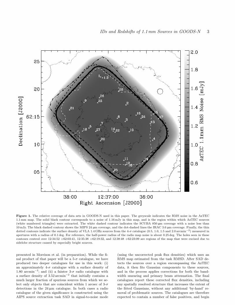
Figure 1. The relative coverage of data sets in GOODS-N used in this paper. The greyscale indicates the RMS noise in the AzTEC1.1mm map. The solid black contour corresponds to a noise of 1.16mJy in this map, and is the region within which AzTEC sources(white numbered triangles) were extracted. The white dashed contour indicates the SCUBA 850 µm coverage with a noise less than10mJy. The black dashed contour shows the MIPS 24 µm coverage, and the dot-dashed lines the IRAC 3.6 µm coverage. Finally, the thindotted contours indicate the surface density of VLA 1.4GHz sources from the 4-σ catalogue (0.5, 1.0, 1.5 and 2.0 arcmin−2) measured inapertures with a radius of 0.1 deg. For reference, the half-power radius of the radio map noise is about 0.25 deg. The holes seen in thesecontours centred over 12:34:52 +62:03:41, 12:35:38 +62:19:32, and 12:38:48 +62:23:09 are regions of the map that were excised due tosidelobe structure caused by especially bright sources.
presented in Morrison et al. (in preparation). While the fi-nal product of that paper will be a 5-σ catalogue, we haveproduced two deeper catalogues for use in this work: (i)an approximately 4-σ catalogue with a surface density of1.80 arcmin−2; and (ii) a fainter 3-σ radio catalogue witha surface density of 3.52 arcmin−2 that initially contains amuch larger fraction of spurious sources from which we se-lect only objects that are coincident within 1 arcsec of 3-σdetections in the 24 µm catalogue. In both cases a radiocatalogue of the given significance is constructed using theAIPS source extraction task SAD in signal-to-noise mode
(using the uncorrected peak flux densities) which uses anRMS map estimated from the task RMSD. After SAD de-tects the sources over a region encompassing the AzTECdata, it then fits Gaussian components to these sources,and in the process applies corrections for both the band-width smearing and primary beam attenuation. The finalcatalogues report these corrected flux densities, includingany spatially resolved structure that increases the extent ofthe fitted Gaussians, without any additional ‘by-hand’ re-moval of problematic sources. The catalogues are thereforeexpected to contain a number of false positives, and begin
4 Edward L. Chapin et al.
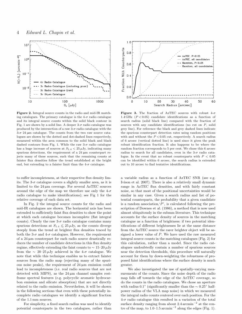
Figure 2. Integral source counts in the radio and mid-IR match-ing catalogues. The primary catalogue is the 4-σ radio catalogueand its integral source counts within the solid black contour inFig. 1 are shown by a solid line. A deeper 3-σ radio catalogue wasproduced by the intersection of a raw 3-σ radio catalogue with the3-σ 24 µm catalogue. The counts from the two raw source cata-logues are shown by the dotted and dot-dashed lines respectively,measured within the area common to the solid black and blackdashed contours from Fig. 1. While the raw 3-σ radio cataloguehas a huge increase of sources at S1.4 < 25 µJy, indicating manyspurious detections, the requirement of a 24 µm counterpart re-jects many of these sources, such that the remaining counts atfainter flux densities follow the trend established at the brightend, but extending to a fainter limit than the 4-σ catalogue.
to suffer incompleteness, at their respective flux density lim-its. The 3-σ catalogue covers a slightly smaller area, as it islimited to the 24 µm coverage. For several AzTEC sourcesaround the edge of the map we therefore use only the 4-σradio catalogue to make identifications); see Fig 1 for therelative coverage of each data set.
In Fig. 2 the integral source counts for the radio andmid-IR catalogues are shown. The horizontal axis has beenextended to sufficiently faint flux densities to show the pointat which each catalogue becomes incomplete (flat integralcounts). Clearly the raw 3-σ radio catalogue contains manyspurious detections at S1.4 <∼ 25 µJy, as the counts divergesteeply from the trend at brighter flux densities traced byboth the 3-σ and 4-σ catalogues. However, the requirementof a 24 µm counterpart for each radio source drastically re-duces the number of candidate detections in this flux densityregime, effectively extending the faint counts to ∼ 15–20 µJyfrom the ∼ 20–25 µJy achieved in the 4-σ catalogue. Wenote that while this technique enables us to extract faintersources from the radio map (rejecting many of the spuri-ous noise peaks), the requirement of 24 µm emission couldlead to incompleteness (i.e. real radio sources that are notdetected with MIPS), as the 24 µm channel samples rest-frame spectral features (e.g. polycyclic aromatic hydrocar-bon emission and silicate absorption) that are not directlyrelated to the radio emission. Nevertheless, it will be shownin the following sections that even with these potentially in-complete radio catalogues we identify a significant fractionof the 1.1 mm sources.
For simplicity, a fixed search radius was used to identifypotential counterparts in the two catalogues, rather than
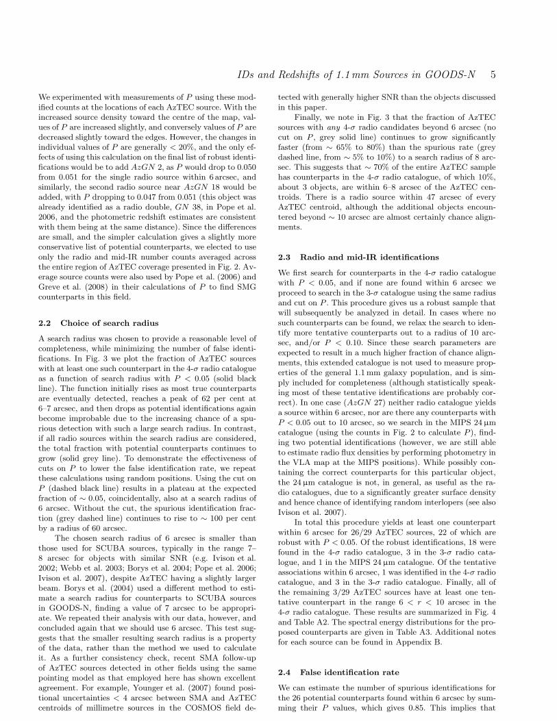
Figure 3. The fraction of AzTEC sources with robust 4-σ1.4GHz (P < 0.05) candidate identifications as a function ofsearch radius (solid black line) compared with the fraction ofsources with any candidate identifications (no cut on P , solidgrey line). For reference the black and grey dashed lines indicatethe spurious counterpart detection rates using random positionswith and without the P < 0.05 cut, respectively. A search radiusof 6 arcsec (vertical dotted line) is used since it gives the peakrobust identification fraction. It also happens to be where therandom fraction corresponds to 5 per cent. We chose this 6 arcsecradius to search for all candidates, even in the 3-σ radio cata-logue. In the event that no robust counterparts with P < 0.05can be identified within 6 arcsec, the search radius is extendedout to 10 arcsec to find tentative identifications.
a variable radius as a function of AzTEC SNR (see e.g.Ivison et al. 2007). There is also a relatively small dynamicrange in AzTEC flux densities, and with fairly constantnoise, so that most of the positional uncertainties would besimilar in any case. Given a search radius and list of po-tential counterparts, the probability that a given candidateis a random association,‘P ’, is calculated following the pre-scription of Downes et al. (1986), a method that is now usedalmost ubiquitously in the submm literature. This techniqueaccounts for the surface density of sources in the matchingcatalogue as a function of brightness: if two potential iden-tifications of different brightnesses lie at the same distancefrom the AzTEC source the rarer brighter object will be as-signed a lower value of P . We have used the raw measuredintegral source counts in the matching catalogues (Fig. 2) forthis calculation, rather than a model. Since the radio cat-alogues undoubtedly contain a number of spurious sourcesnear the detection thresholds, this procedure will naturallyaccount for them by down-weighting the robustness of pro-posed faint identifications where the surface density is muchgreater.
We also investigated the use of spatially-varying mea-surements of the counts. Since the noise depth of the radiomap falls off towards the edge of the AzTEC coverage, sodo the counts in the radio catalogues. We chose an aperturewith radius 0.1◦ (significantly smaller than the ∼ 0.25◦ half-power radius of the VLA map noise) in which we measuredthe integral radio counts centered over each position. For the4-σ radio catalogue this resulted in a variation of the totalsurface density ranging from about 2.4 arcmin−2 at the cen-tre of the map, to 1.0–1.5 arcmin−2 along the edges (Fig. 1).
IDs and Redshifts of 1.1mm Sources in GOODS-N 5
We experimented with measurements of P using these mod-ified counts at the locations of each AzTEC source. With theincreased source density toward the centre of the map, val-ues of P are increased slightly, and conversely values of P aredecreased slightly toward the edges. However, the changes inindividual values of P are generally < 20%, and the only ef-fects of using this calculation on the final list of robust identi-fications would be to add AzGN 2, as P would drop to 0.050from 0.051 for the single radio source within 6 arcsec, andsimilarly, the second radio source near AzGN 18 would beadded, with P dropping to 0.047 from 0.051 (this object wasalready identified as a radio double, GN 38, in Pope et al.2006, and the photometric redshift estimates are consistentwith them being at the same distance). Since the differencesare small, and the simpler calculation gives a slightly moreconservative list of potential counterparts, we elected to useonly the radio and mid-IR number counts averaged acrossthe entire region of AzTEC coverage presented in Fig. 2. Av-erage source counts were also used by Pope et al. (2006) andGreve et al. (2008) in their calculations of P to find SMGcounterparts in this field.
2.2 Choice of search radius
A search radius was chosen to provide a reasonable level ofcompleteness, while minimizing the number of false identi-fications. In Fig. 3 we plot the fraction of AzTEC sourceswith at least one such counterpart in the 4-σ radio catalogueas a function of search radius with P < 0.05 (solid blackline). The function initially rises as most true counterpartsare eventually detected, reaches a peak of 62 per cent at6–7 arcsec, and then drops as potential identifications againbecome improbable due to the increasing chance of a spu-rious detection with such a large search radius. In contrast,if all radio sources within the search radius are considered,the total fraction with potential counterparts continues togrow (solid grey line). To demonstrate the effectiveness ofcuts on P to lower the false identification rate, we repeatthese calculations using random positions. Using the cut onP (dashed black line) results in a plateau at the expectedfraction of ∼ 0.05, coincidentally, also at a search radius of6 arcsec. Without the cut, the spurious identification frac-tion (grey dashed line) continues to rise to ∼ 100 per centby a radius of 60 arcsec.
The chosen search radius of 6 arcsec is smaller thanthose used for SCUBA sources, typically in the range 7–8 arcsec for objects with similar SNR (e.g. Ivison et al.2002; Webb et al. 2003; Borys et al. 2004; Pope et al. 2006;Ivison et al. 2007), despite AzTEC having a slightly largerbeam. Borys et al. (2004) used a different method to esti-mate a search radius for counterparts to SCUBA sourcesin GOODS-N, finding a value of 7 arcsec to be appropri-ate. We repeated their analysis with our data, however, andconcluded again that we should use 6 arcsec. This test sug-gests that the smaller resulting search radius is a propertyof the data, rather than the method we used to calculateit. As a further consistency check, recent SMA follow-upof AzTEC sources detected in other fields using the samepointing model as that employed here has shown excellentagreement. For example, Younger et al. (2007) found posi-tional uncertainties < 4 arcsec between SMA and AzTECcentroids of millimetre sources in the COSMOS field de-
tected with generally higher SNR than the objects discussedin this paper.
Finally, we note in Fig. 3 that the fraction of AzTECsources with any 4-σ radio candidates beyond 6 arcsec (nocut on P , grey solid line) continues to grow significantlyfaster (from ∼ 65% to 80%) than the spurious rate (greydashed line, from ∼ 5% to 10%) to a search radius of 8 arc-sec. This suggests that ∼ 70% of the entire AzTEC samplehas counterparts in the 4-σ radio catalogue, of which 10%,about 3 objects, are within 6–8 arcsec of the AzTEC cen-troids. There is a radio source within 47 arcsec of everyAzTEC centroid, although the additional objects encoun-tered beyond ∼ 10 arcsec are almost certainly chance align-ments.
2.3 Radio and mid-IR identifications
We first search for counterparts in the 4-σ radio cataloguewith P < 0.05, and if none are found within 6 arcsec weproceed to search in the 3-σ catalogue using the same radiusand cut on P . This procedure gives us a robust sample thatwill subsequently be analyzed in detail. In cases where nosuch counterparts can be found, we relax the search to iden-tify more tentative counterparts out to a radius of 10 arc-sec, and/or P < 0.10. Since these search parameters areexpected to result in a much higher fraction of chance align-ments, this extended catalogue is not used to measure prop-erties of the general 1.1 mm galaxy population, and is sim-ply included for completeness (although statistically speak-ing most of these tentative identifications are probably cor-rect). In one case (AzGN 27) neither radio catalogue yieldsa source within 6 arcsec, nor are there any counterparts withP < 0.05 out to 10 arcsec, so we search in the MIPS 24 µmcatalogue (using the counts in Fig. 2 to calculate P ), find-ing two potential identifications (however, we are still ableto estimate radio flux densities by performing photometry inthe VLA map at the MIPS positions). While possibly con-taining the correct counterparts for this particular object,the 24 µm catalogue is not, in general, as useful as the ra-dio catalogues, due to a significantly greater surface densityand hence chance of identifying random interlopers (see alsoIvison et al. 2007).
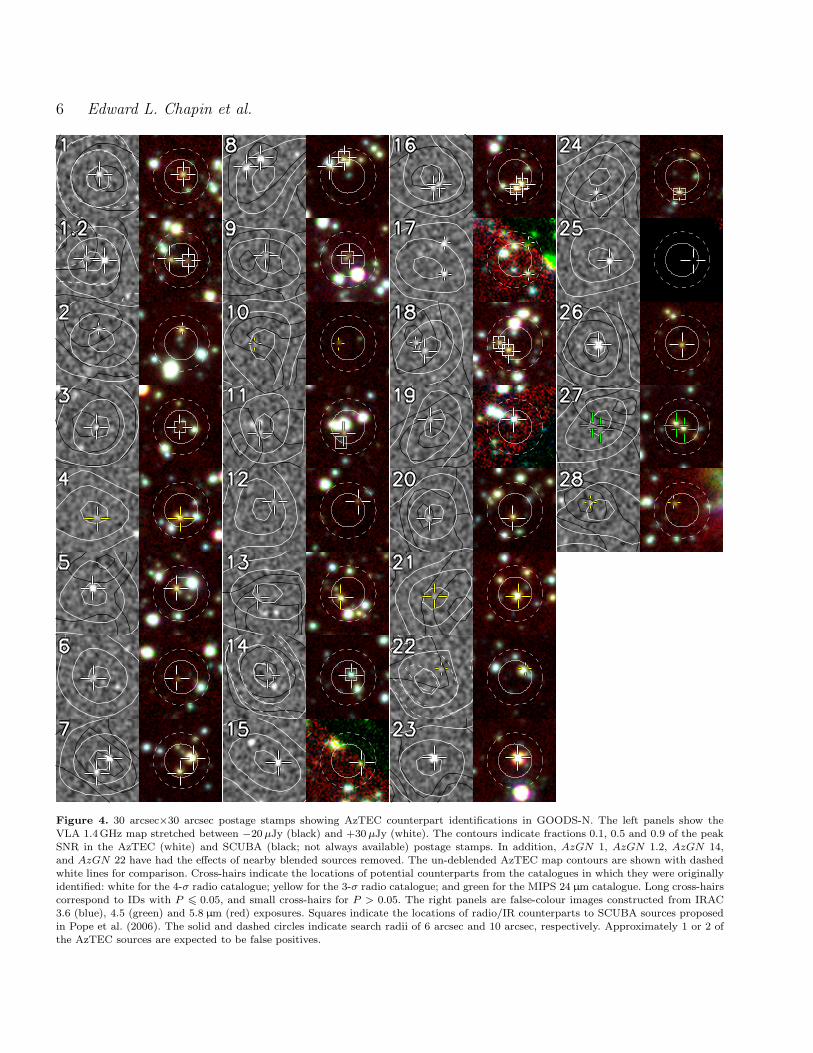
In total this procedure yields at least one counterpartwithin 6 arcsec for 26/29 AzTEC sources, 22 of which arerobust with P < 0.05. Of the robust identifications, 18 werefound in the 4-σ radio catalogue, 3 in the 3-σ radio cata-logue, and 1 in the MIPS 24 µm catalogue. Of the tentativeassociations within 6 arcsec, 1 was identified in the 4-σ radiocatalogue, and 3 in the 3-σ radio catalogue. Finally, all ofthe remaining 3/29 AzTEC sources have at least one ten-tative counterpart in the range 6 < r < 10 arcsec in the4-σ radio catalogue. These results are summarized in Fig. 4and Table A2. The spectral energy distributions for the pro-posed counterparts are given in Table A3. Additional notesfor each source can be found in Appendix B.
2.4 False identification rate
We can estimate the number of spurious identifications forthe 26 potential counterparts found within 6 arcsec by sum-ming their P values, which gives 0.85. This implies that
6 Edward L. Chapin et al.
Figure 4. 30 arcsec×30 arcsec postage stamps showing AzTEC counterpart identifications in GOODS-N. The left panels show theVLA 1.4GHz map stretched between −20 µJy (black) and +30 µJy (white). The contours indicate fractions 0.1, 0.5 and 0.9 of the peakSNR in the AzTEC (white) and SCUBA (black; not always available) postage stamps. In addition, AzGN 1, AzGN 1.2, AzGN 14,and AzGN 22 have had the effects of nearby blended sources removed. The un-deblended AzTEC map contours are shown with dashedwhite lines for comparison. Cross-hairs indicate the locations of potential counterparts from the catalogues in which they were originallyidentified: white for the 4-σ radio catalogue; yellow for the 3-σ radio catalogue; and green for the MIPS 24 µm catalogue. Long cross-hairscorrespond to IDs with P 6 0.05, and small cross-hairs for P > 0.05. The right panels are false-colour images constructed from IRAC3.6 (blue), 4.5 (green) and 5.8 µm (red) exposures. Squares indicate the locations of radio/IR counterparts to SCUBA sources proposedin Pope et al. (2006). The solid and dashed circles indicate search radii of 6 arcsec and 10 arcsec, respectively. Approximately 1 or 2 ofthe AzTEC sources are expected to be false positives.
IDs and Redshifts of 1.1mm Sources in GOODS-N 7
of those 26 AzTEC sources, about one of the identifica-tions within 6 arcsec is expected to be spurious (noting thatseveral sources have multiple proposed identifications). Tounderstand how to interpret this result in terms of overallcompleteness, we consider several factors. First, the AzTECsource list is expected to have ∼ 1–2 spurious detections(Perera et al. 2008). Second, due to positional uncertainties,some of the true counterparts will lie beyond 6 arcsec. Weadopt the radial offset distribution of Ivison et al. (2007),r exp(−r2/2σ2), with σ ∼ 0.6 × FWHM/SNR, which as-sumes a symmetric Gaussian beam and uncorrelated mapnoise. The cumulative distribution of this analytic PDF re-sults in a shape very similar to the numerical simulationsof Scott et al. (2008) for AzTEC sources in the COSMOSfield. Taking FWHM = 18 arcsec, and the SNR for raw mapflux densities (before deboosting), we would only expect toencounter counterparts within 6 arcsec for 27.5/29 sourceson average if they were all real (neglecting positional un-certainties in the matching catalogue). However, we wouldconfidently expect to find all of the objects within 10 arc-sec. Since we do not know which (if any) of the AzTECsources are false positives, we simply apply this fraction tothe expected number of real sources calculated above, andfind that there should be ∼ 26–27 real sources with truepositions within 6 arcsec of their 1.1mm centroids. This ex-pectation is consistent with our identification rate within6 arcsec of ∼ 25–26 out of 29 sources, although we stress thatthis statistical argument does not necessarily imply that theunmatched sources are spurious. We find P values less than0.05 for only 21 of the sources encountered within 6 arcsec(excluding AzGN 14 as noted below). While it may be thecase that most of the remaining 5 sources are in fact asso-ciated with the 1.1 mm objects, it is also possible that thetrue counterparts are simply fainter in the radio than thecatalogue limit. We cannot distinguish between these twocases in the present study given the positional uncertaintiesin the AzTEC centroids.
As a final warning, as with all studies that use P toevaluate chance alignment probabilities, there is an under-lying assumption that the matching catalogues are spatiallyunclustered. Two examples of ways in which this conditioncould be broken are an increased surface density of sourcesin the vicinity of SMGs due to multiple catalogue entries be-ing associated with the same physical structure (such as agalaxy cluster), or foreground lensing of background objects(an effect which is in fact commonly used to identify faintSMGs, e.g. Smail et al. 2002). In both of these cases P wouldbe biased low. We do not attempt to correct for these effectsin this work, but we alert the reader that evidence for suchcases in GOODS-N will be discussed in the following sec-tions: the particularly complicated identification of a coun-terpart for AzGN 14 (also known HDF 850.1, Hughes et al.1998) which caused us to drop it from the analysis in this pa-per; and the potential presence of a protocluster at redshiftz ∼ 4.
2.5 Comparison with SCUBA identifications
Since 12 of the 29 objects discussed in this paper were alsodetected by SCUBA (see Table A2) and identified in the ra-dio and mid-IR using similar techniques (Pope et al. 2006;Wall et al. 2008), it is useful to compare proposed identifica-
tions to see how the new AzTEC positions and deeper radiocatalogues affect the results. We exclude AzGN 14/GN 14(HDF 850.1) from this comparison (and most of the re-maining analysis in this paper) as its true counterpart hasbeen under debate for some time due to the suspected ob-scuration by a foreground elliptical (see Dunlop et al. 2004;Cowie et al. 2009, and notes in Appendix B). Of the re-maining 11 overlapping sources, we propose identical coun-terparts for 8 of those objects. For AzGN 1.2 we findthat both the proposed counterpart of Pope et al. (2006)(P = 0.005 in this paper) and a second fainter radio ob-ject (with P = 0.037, also noted by Daddi et al. 2008) areboth robust identifications by our definition. In another sim-ilar case, only one object from a radio double identified byPope et al. (2006) for AzGN 18 is strictly a robust coun-terpart (P = 0.032 in this paper), while the second radiosource misses the cut, with P = 0.051. The only objectfor which we propose a completely different counterpart isAzGN 11/GN 27, which was classified as ‘tentative’ in theSCUBA map: the ACS/IRAC identification from Pope et al.(2006) is absent in the 1.4 GHz map, and we instead proposea radio source that lies slightly to the north, with P = 0.027.
3 REDSHIFT DISTRIBUTION
Some recent surveys at 1.1–1.2 mm claim to detecthigher redshifts than SCUBA surveys at 850 µm (e.g.Younger et al. 2007; Greve et al. 2008), while others findredshift distributions that are indistinguishable, possi-bly due to small samples sizes (e.g. Greve et al. 2004;Bertoldi et al. 2007). For this AzTEC survey we more accu-rately quantify any differences using greatly improved red-shift information, and comparing directly to the SCUBAresults in this field using the same methodology. While theuncertainty in the 1.1 mm distribution derived from our datais large, due to the relatively small sample size, and cosmicvariance resulting from the area of GOODS-N, this differ-ential measurement yields a useful comparison between thetwo bands.
A number of groups have obtained spectroscopic red-shifts in GOODS-N (e.g. Cohen et al. 2000; Cowie et al.2004; Wirth et al. 2004; Chapman et al. 2005; Reddy et al.2006; Barger et al. 2008; Pope et al. 2008; Daddi et al. 2008,2009, Stern et al. in preparation). We found spectroscopicredshifts for 10 of our proposed AzTEC counterparts inthese publicly available data-sets (see Table A2). However,one of those redshifts (AzGN 8) corresponds to the leastfavourable counterpart within the search radius (see thediscussion for this source in Appendix B). Another simi-lar case is AzGN 27 for which a spectroscopic redshift hasbeen obtained only for the more distant of two potentialcounterparts. Finally, two radio sources that appear to beassociated with the single object AzGN 7 lie at redshiftsz = 1.996 and z = 1.992, and we assign a single redshift ofz = 1.994, which is sufficiently precise for the purposes ofthis paper. Therefore our sample of 21 sources with unam-biguous identifications contains only 7/21 sources with spec-troscopic redshifts. This fraction is considerably lower thanthe 15/20 spectroscopic redshifts for robust counterpartsfrom the Pope et al. (2006) SCUBA sample (also excludingHDF 850.1), including the two new redshifts for GN 20 and
8 Edward L. Chapin et al.
GN 20.2 from Daddi et al. (2008), the redshift for GN 10from Daddi et al. (2009) and two additional Spitzer IRS red-shifts from Pope et al. (2008). However, we are not surprisedat this lower rate since we rely on archival data for the red-shifts of counterparts to new AzTEC sources, whereas manyof the spectroscopic redshifts for SCUBA sources were ob-tained using targeted follow-up of proposed identifications.
For sources without a spectroscopic redshift we firstsearched for optical photometric redshift estimates. As nonewere found, we instead employed two photometric redshiftcalculations using longer wavelength data. The first, zir, is asimple function of the Spitzer photometry with coefficientsderived from fits to SCUBA sources in GOODS-N with spec-troscopic redshifts (Pope et al. 2006). Although this methoddoes not assume any particular SED, it benefits from the1.6 µm stellar bump that produces a strong characteristicfeature in the observed IRAC 3.6–8.0 µm bands for sourcesat redshifts 1 <∼ z <∼ 4 (Simpson & Eisenhardt 1999; Sawicki2002). Such an empirical calculation may provide less bi-ased results than fitting spectral templates to the data sincethere are degeneracies between the derived redshift and as-sumptions about the starburst producing the stellar bump(see discussion in Yun et al. 2008). While the residuals forthis functional fit are relatively small (with a maximum∆z = 0.4), no uncertainties are provided in Pope et al.(2006) for the remaining sources. However, a similar pho-tometric redshift estimator was derived by Wilson et al.(2008), and a comparison with spectroscopic redshifts forSMGs from several fields (including SCUBA sources fromboth GOODS-N and SHADES) finds that a 1-σ error enve-lope ∆z = 0.15(1 + z) is a reasonable uncertainty estimatefor 15 SMGs at redshifts 0 <∼ z <∼ 3. We have comparedthe Pope et al. (2006) and Wilson et al. (2008) photometricredshift formulae for our data and find that of the 7 ro-bust identifications with spectroscopic redshifts both meth-ods provide estimates consistent with the spectroscopic mea-surements for the 3 sources at z < 3, within the Wilson et al.(2008) error envelope. However, both estimates are biasedlow at z > 3, more so using the Wilson et al. (2008) red-shift estimator. We also checked the scatter between the twomethods for all of the robust identifications finding that theyboth gave answers compatible with the Wilson et al. (2008)uncertainty estimate. This bias and scatter are unsurprisingas both formulae were fit to SMGs with spectroscopic red-shifts z <∼ 3. In this work we assume the 1-σ uncertaintiesare also ∆zir = 0.15(1 + z), but warn the reader that theredshifts of more distant objects are probably systematicallyunderestimated with this technique.
The second photometric redshift indicator, zrm, uses theradio and (sub)mm flux densities fit to templates of localgalaxies assuming the radio-IR correlation holds at high red-shift (e.g. Carilli & Yun 1999; Aretxaga et al. 2007). Thismethod provides the only redshift estimates for a handful ofsources around the edges of the AzTEC map where there isno Spitzer or optical coverage from the GOODS survey (theentire AzTEC survey area overlaps with the 1.4 GHz data).Our redshifts are calculated using the same methodologyas Aretxaga et al. (2007) and summarized in Table A2. Wenote that the quoted 68 per cent confidence intervals aretheoretical estimations; Aretxaga et al. (2007) checked thescatter between photometric and spectroscopic redshifts fora sample of SMGs with radio and submm data of similar
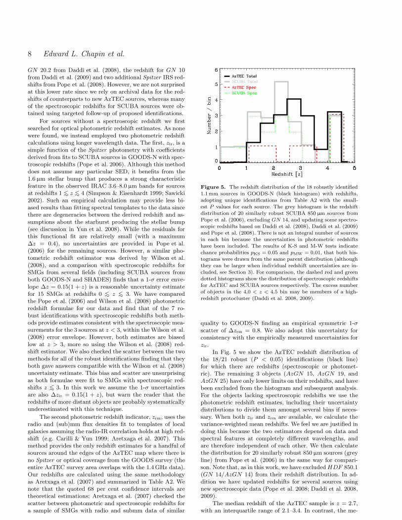
Figure 5. The redshift distribution of the 18 robustly identified1.1mm sources in GOODS-N (black histogram) with redshifts,adopting unique identifications from Table A2 with the small-est P values for each source. The grey histogram is the redshiftdistribution of 20 similarly robust SCUBA 850 µm sources fromPope et al. (2006), excluding GN 14, and updating some spectro-scopic redshifts based on Daddi et al. (2008), Daddi et al. (2009)and Pope et al. (2008). There is not an integral number of sourcesin each bin because the uncertainties in photometric redshiftshave been included. The results of K-S and M-W tests indicatechance probabilities pKS = 0.05 and pMW = 0.01, that both his-tograms were drawn from the same parent distribution (althoughthey can be larger when individual redshift uncertainties are in-cluded, see Section 3). For comparison, the dashed red and greendotted histograms show the distribution of spectroscopic redshiftsfor AzTEC and SCUBA sources respectively. The excess numberof objects in the 4.0 < z < 4.5 bin may be members of a high-redshift protocluster (Daddi et al. 2008, 2009).
quality to GOODS-N finding an empirical symmetric 1-σscatter of ∆zrm = 0.8. We also adopt this uncertainty forconsistency with the empirically measured uncertainties forzir.
In Fig. 5 we show the AzTEC redshift distribution ofthe 18/21 robust (P < 0.05) identifications (black line)for which there are redshifts (spectroscopic or photomet-ric). The remaining 3 objects (AzGN 15, AzGN 19, andAzGN 25) have only lower limits on their redshifts, and havebeen excluded from the histogram and subsequent analysis.For the objects lacking spectroscopic redshifts we use thephotometric redshift estimates, including their uncertaintydistributions to divide them amongst several bins if neces-sary. When both zir and zrm are available, we calculate thevariance-weighted mean redshifts. We feel we are justified indoing this because the two estimators depend on data andspectral features at completely different wavelengths, andare therefore independent of each other. We then calculatethe distribution for 20 similarly robust 850 µm sources (greyline) from Pope et al. (2006) in the same way for compari-son. Note that, as in this work, we have excluded HDF 850.1(GN 14/AzGN 14) from their redshift distribution. In ad-dition we have updated redshifts for several sources usingnew spectroscopic data (Pope et al. 2008; Daddi et al. 2008,2009).
The median redshift of the AzTEC sample is z = 2.7,with an interquartile range of 2.1–3.4. In contrast, the me-
IDs and Redshifts of 1.1mm Sources in GOODS-N 9
dian of the SCUBA sample shown here is z = 2.0 with aninterquartile range 1.3–2.6. For reference, the 14 SCUBAsources with spectroscopic redshifts (green dotted histogramin Fig. 5) has a median z = 2.0, and the 7 AzTEC sources(red dashed histogram) z = 3.19, both in good agreementwith the full distributions despite the small numbers of ob-jects. It is also worth noting that the spike of spectroscopicredshifts in the 4.0 < z < 4.5 bin seen at both wavelengthswas found via targeted follow-up to SCUBA sources byDaddi et al. (2008) and Daddi et al. (2009) that are thoughtto be members of a proposed protocluster at z ∼ 4. Al-though not included in the distribution, a recent study byCowie et al. (2009) suggests that HDF 850.1 may also be amember of this high-redshift structure.
We note that while the AzTEC sample appears to lieat slightly higher redshift than the SCUBA sample, we havehad to rely more heavily on highly uncertain photometricestimates than in Pope et al. (2006). However, the bias islikely to be toward lower rather than higher redshifts due tothe nature of zir.
Next, taking the SCUBA and AzTEC redshift distribu-tions at face value (including photometric redshifts) we haveused the Kolmogorov-Smirnov (K-S) and Mann-Whitney U(M-W) non-parametric tests for assessing how different theyare. These tests are fair since both samples were drawn fromthe same region of space, and no extra uncertainty needs tobe included to account for cosmic variance. Both methodsoperate on discrete samples so we first assign the mean red-shift to each object from its uncertainty distribution. TheK-S test, which is sensitive to more general differences inthe distributions (both the central values and tails), gives achance probability pKS = 0.05 that both samples were drawnfrom the same parent redshift distribution. The M-W test,which is mostly sensitive to differences in the central val-ues of the distributions, gives a smaller chance probabilitypMW = 0.01. However, we note that the uncertainties for ob-jects with photometric redshifts can be as large as ∆z ∼ 0.8,comparable to the width of the entire population. To evalu-ate the spread in K-S and M-W probabilities that are con-sistent with our sample, we generate 10,000 mock samplesat each wavelength drawing individual redshifts at randomfrom the uncertainty distributions for each object. We findthat 68 per cent of the time we obtain values pKS < 0.15and pMW < 0.04. These tests show that, even with large in-dividual uncertainties, the shift to higher redshifts at 1.1mmcompared to 850 µm appears to be statistically significant.
The SCUBA sample consists of a broader dynamicrange in flux density than the AzTEC sample, due to thevarying map depths, and the fact that different redshift pop-ulations may be present in the deep and shallow regions ofthe map (Pope et al. 2006; Wall et al. 2008). It thereforemay be the case that at least some of the differences be-tween these distributions are a result of a depth rather thanwavelength selection effect.
One potential concern with this comparison is that, dueto a bias to higher redshifts at fainter flux densities (e.g.Chapman et al. 2005), the deeper radio catalogues used formatching in this survey simply detect more distant poten-tial counterparts than in Pope et al. (2006). We checked thedistribution of radio brightness with redshift for our sampleand found that the 6 faintest proposed radio counterpartslie in the redshift interval 2 < z < 3. Removing them, while
broadening the remaining redshift distribution slightly, doesnot shift the median appreciably. However, if we removesources with even brighter radio flux densities, we in fact be-gin to bias the sample to higher redshifts. Combined with thefact that we find most of the same counterparts for sourcesthat appear in both the AzTEC and SCUBA surveys (Sec-tion 2.5), we conclude that the intrinsic rest-frame scatterof radio luminosities in SMGs dominates any differences inthe radio properties of 850 µm and 1.1 mm selected samples.
The lowest redshift that we find is AzGN 23 at z =1.146. This demonstrates the ability of mm-wavelength sur-veys to effectively select galaxies at z > 1, with little con-tamination from nearby objects. Assuming that our iden-tification procedure and redshift estimates are correct, andgiven the completeness of our survey, there is therefore lit-tle room for a significant tail to extremely high redshifts.Since the negative K-correction at 1.1 mm could in princi-ple enable us to detect SMGs easily out to a redshift z ∼ 10(Blain et al. 2002), the fact that objects at z >∼ 4.5 do notappear in our sample demonstrates that they do not existin large quantities, and would therefore require much largersurveys to find them. Only if many of the identifications forthese AzTEC sources are in fact more complicated (as inthe case of HDF 850.1) may the door still be open for a sig-nificant fraction of the SMG population to lie at generallyhigher redshifts (z > 4.5).
4 SPECTRAL ENERGY DISTRIBUTIONS
With redshift estimates in hand, we are now in a posi-tion to probe the rest-frame SEDs of our sample. Althoughwe have photometry at a number of wavelengths spanning3.6 µm to 20 cm for most of the objects, the most inter-esting new constraints that we place on these SEDs is theshape of their rest-frame far-IR emission that peaks near100 µm in the rest-frame, produced by thermal dust grainemission. This emission accounts for most of the bolometricluminosity in SMGs, and it is generally believed to be pro-duced by optically-obscured star formation in most cases(e.g. Blain et al. 2002), much like locally observed ULIRGs.The far-IR luminosity is therefore crucial for estimating star-formation rates. The far-IR SED also provides a direct probeof the total dust mass in a galaxy. However, both the bolo-metric luminosity and dust mass are critically dependenton the dust temperature, T , and the dust grain emissiv-ity, β (Hildebrand 1983). Due to a dearth of data at thenecessary wavelengths, spanning ∼ 100–1000 µm, most au-thors either attempt to fit a simple 3-parameter modifiedblackbody spectrum for a population of dust grains at asingle temperature, Sν = AνβBν(T ) (where A is the am-plitude), or adopt a single SED and normalize it to the(sub)mm data point. Since only a single (sub)mm datapoint is usually available, this latter compromise is oftenmade. A census of recent studies finds broad agreementthat the most typical values are Td = 30–35 K for SMGs,with an allowed range that is somewhat broader than this(Chapman et al. 2005; Kovacs et al. 2006; Pope et al. 2006;Huynh et al. 2007; Coppin et al. 2008). However, the esti-mates of Td and β are highly correlated, because of the lim-ited range of wavelengths for which data exist.
In GOODS-N the combination of 1.1mm and 850 µm
10 Edward L. Chapin et al.
flux densities sample wavelengths longward of the rest-framefar-IR peak. The ratio S850/S1.1 defines a family of 2-parameter SEDs (T and β) for each source which we willuse to check for consistency with previous measurements ofthe thermal SEDs of SMGs at typically shorter wavelengths.
4.1 Correcting for flux density bias
We first estimate un-biased 1.1 mm and 850 µm flux den-sities for the AzTEC sources. As discussed in Perera et al.(2008), the 1.1 mm flux densities are biased high becausethey are selected from a low SNR list of peaks coming from acounts distribution that falls steeply with increasing bright-ness. The correction for this bias followed the prescriptionof Coppin et al. (2005), and we adopt those posterior fluxdensity distributions here. While this correction does not ac-count for the additional effect of source blending, the AzTECGOODS-N survey is shallower than the estimated confusionlimit, and the sources that appear to be confused have beenfit explicitly in this paper using two components. Ratherthan cross-matching the AzTEC catalogue with the SCUBAcatalogue to obtain 850 µm flux densities, which itself suffersflux density bias (and since the SCUBA data are also tooshallow in some areas to provide flux densities for many ofour sources), we instead directly measure the 850 µm map atthe positions of proposed counterparts. Provided that thesecounterparts are correct, and 850 µm source confusion is neg-ligible, this photometry yields un-biased 850 µm flux den-sities with symmetric Gaussian uncertainties for all 24/29AzTEC sources that land within the region of SCUBA cov-erage. However, due to the wide range in sensitivities only9 objects have 850 µm detections with a significance of atleast 3-σ.
4.2 Searching for ‘850 µm dropouts’
It has been suggested that in regions where observationsat both 850 µm and ∼1.1 mm exist ‘850 µm dropouts’,i.e. sources that are detected by AzTEC but not by SCUBA,can be used to select predominantly higher-redshift sources(Greve et al. 2004, 2008). This technique is expected to workfor the same reason that the AzTEC redshift distributionis slightly higher than the SCUBA sample: there is an in-creased submm negative K-correction at 1.1 mm comparedto 850 µm (i.e. the ratio of 850 µm to 1.2 mm flux density,S850/S1.2, decreases with redshift, seen for example in Fig-ure 4 of Eales et al. 2003). In this study, we proceed by firsttesting the hypothesis of a single intrinsic observed flux den-sity ratio R ≡ S850/S1.1, by measuring R for several high-SNR objects selected in the AzTEC map, and then search-ing for dropouts in the SCUBA map relative to this averagecolour. We also repeat this analysis in the opposite direc-tion (for completeness), searching for SCUBA sources thatare dropouts in the AzTEC map.
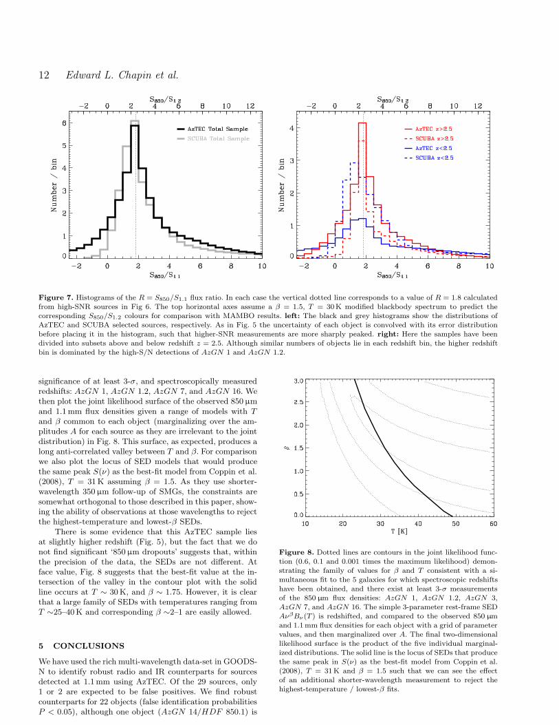
We measure R using sources with deboosted flux den-sities that have significances > 3-σ in both bands: AzGN 1,AzGN 3, AzGN 7 and AzGN 8, giving similar values 1.72,1.96, 1.67 and 2.04 respectively. We adopt the mean R = 1.8.For reference, thermal emission from a galaxy with T = 30 Kand β = 1.5 at z = 2.5 would give an observed ratio 1.85.In order to compare our measurement with values reported
for SCUBA (850 µm) and MAMBO (1.2 mm) overlap, weuse the same model SED to estimate how much larger theS850/S1.2 ratio would be, finding that the scaled result is 2.3,near the centre of the distributions reported by Greve et al.(2004, 2008). Similarly we scale our result to estimate the ra-tio S890/S1.1 for 890 µm SMA follow-up of AzTEC sources,finding a ratio of 1.6. This value is consistent with 1.4± 0.3reported by Younger et al. (2007).
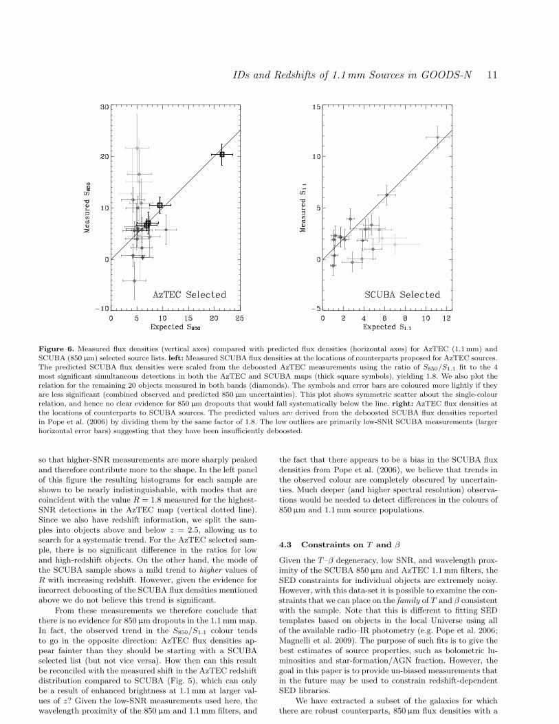
Next we use our measured R to scale the deboosted1.1 mm flux density distributions for the entire sample to850 µm. For simplicity we approximate the scaled 850 µmpredicted flux density distributions as Gaussians with meanvalues sm given by the modes, and standard deviations σm
as half of the 68 per cent confidence intervals. If our hypoth-esis of a single observed ratio were true, given the observed850 µm data with mean flux densities sd and standard devia-tions σd, we would expect the residuals (sm−sd)/
√
σ2m + σ2
d
to be normally distributed with mean 0 and standard devi-ation 1. For the 20 objects that do not have 3-σ detectionsat 850µm we calculate the sample mean and standard de-viation of the residuals, giving −0.1 ± 1.4. This calculationconfirms that a ratio of 1.8 is a good estimate for the cen-tral value of the observed distribution S850/S1.1 (left panelof Fig. 6).
Since the residual is broader than expected (by a factor∼
√2), we conclude that the intrinsic spread in R produces
uncertainties of the same order as our measurement errors.Note that the spread in R for a T = 30 K, β = 1.5 SEDfrom redshifts z = 1–4 is only 2.1–1.6, so that part of themeasured spread must be due to a range of rest-frame dustemission spectra in addition to the redshift distribution. Wenote that this scatter is roughly symmetric: the 850 µm mea-surements fall above the expected values about as often asthey fall below (in the left panel of Fig. 6).
These calculations are biased to 1.1 mm selectedsources, and could in principle be different for an 850 µmselected catalogue. We therefore repeat the procedure, start-ing with deboosted flux densities for the 20 robustly iden-tified SCUBA sources mentioned in Section 3, scaling themto 1.1mm by dividing them by R, and comparing these pre-dictions to photometry at the locations of their counter-parts in the AzTEC map (right panel of Fig. 6). In thiscase the scatter is clearly asymmetric, with a number ofthe SCUBA sources appearing fainter than expected in theAzTEC map. However, these outliers are primarily low-SNRSCUBA detections (indicated by the large horizontal errorbars), in particular GN 3, GN 5, GN 7, GN 16 and GN 22which have uncertainties ranging from 1.5–4.5 mJy. We hy-pothesize that the Pope et al. (2006) deboosting recipe didnot sufficiently correct these sources, i.e. they should havebeen shifted further to the left in this plot. This explanationis plausible because their deboosting factors were extrapo-lated from those calculated for the SCUBA SHADES survey(Coppin et al. 2006), which were derived for sources with adifferent noise distribution. Furthermore, the fact that theAzTEC selected source list does not exhibit this problem(left panel of Fig. 6) also points to an issue with the SCUBAdeboosting calculation, rather than the map itself.
Finally, we use the AzTEC and SCUBA selected sourcelists to plot histograms of the measured S850/S1.1 flux ratiosin Fig. 7. Here we have convolved each source with its uncer-tainty distribution before adding it to the total histogram,
IDs and Redshifts of 1.1mm Sources in GOODS-N 11
Figure 6. Measured flux densities (vertical axes) compared with predicted flux densities (horizontal axes) for AzTEC (1.1mm) andSCUBA (850 µm) selected source lists. left: Measured SCUBA flux densities at the locations of counterparts proposed for AzTEC sources.The predicted SCUBA flux densities were scaled from the deboosted AzTEC measurements using the ratio of S850/S1.1 fit to the 4most significant simultaneous detections in both the AzTEC and SCUBA maps (thick square symbols), yielding 1.8. We also plot therelation for the remaining 20 objects measured in both bands (diamonds). The symbols and error bars are coloured more lightly if theyare less significant (combined observed and predicted 850 µm uncertainties). This plot shows symmetric scatter about the single-colourrelation, and hence no clear evidence for 850 µm dropouts that would fall systematically below the line. right: AzTEC flux densities atthe locations of counterparts to SCUBA sources. The predicted values are derived from the deboosted SCUBA flux densities reportedin Pope et al. (2006) by dividing them by the same factor of 1.8. The low outliers are primarily low-SNR SCUBA measurements (largerhorizontal error bars) suggesting that they have been insufficiently deboosted.
so that higher-SNR measurements are more sharply peakedand therefore contribute more to the shape. In the left panelof this figure the resulting histograms for each sample areshown to be nearly indistinguishable, with modes that arecoincident with the value R = 1.8 measured for the highest-SNR detections in the AzTEC map (vertical dotted line).Since we also have redshift information, we split the sam-ples into objects above and below z = 2.5, allowing us tosearch for a systematic trend. For the AzTEC selected sam-ple, there is no significant difference in the ratios for lowand high-redshift objects. On the other hand, the mode ofthe SCUBA sample shows a mild trend to higher values ofR with increasing redshift. However, given the evidence forincorrect deboosting of the SCUBA flux densities mentionedabove we do not believe this trend is significant.
From these measurements we therefore conclude thatthere is no evidence for 850 µm dropouts in the 1.1 mm map.In fact, the observed trend in the S850/S1.1 colour tendsto go in the opposite direction: AzTEC flux densities ap-pear fainter than they should be starting with a SCUBAselected list (but not vice versa). How then can this resultbe reconciled with the measured shift in the AzTEC redshiftdistribution compared to SCUBA (Fig. 5), which can onlybe a result of enhanced brightness at 1.1 mm at larger val-ues of z? Given the low-SNR measurements used here, thewavelength proximity of the 850 µm and 1.1 mm filters, and
the fact that there appears to be a bias in the SCUBA fluxdensities from Pope et al. (2006), we believe that trends inthe observed colour are completely obscured by uncertain-ties. Much deeper (and higher spectral resolution) observa-tions would be needed to detect differences in the colours of850 µm and 1.1 mm source populations.
4.3 Constraints on T and β
Given the T–β degeneracy, low SNR, and wavelength prox-imity of the SCUBA 850 µm and AzTEC 1.1 mm filters, theSED constraints for individual objects are extremely noisy.However, with this data-set it is possible to examine the con-straints that we can place on the family of T and β consistentwith the sample. Note that this is different to fitting SEDtemplates based on objects in the local Universe using allof the available radio–IR photometry (e.g. Pope et al. 2006;Magnelli et al. 2009). The purpose of such fits is to give thebest estimates of source properties, such as bolometric lu-minosities and star-formation/AGN fraction. However, thegoal in this paper is to provide un-biased measurements thatin the future may be used to constrain redshift-dependentSED libraries.
We have extracted a subset of the galaxies for whichthere are robust counterparts, 850 µm flux densities with a
12 Edward L. Chapin et al.
Figure 7. Histograms of the R = S850/S1.1 flux ratio. In each case the vertical dotted line corresponds to a value of R = 1.8 calculatedfrom high-SNR sources in Fig 6. The top horizontal axes assume a β = 1.5, T = 30K modified blackbody spectrum to predict thecorresponding S850/S1.2 colours for comparison with MAMBO results. left: The black and grey histograms show the distributions ofAzTEC and SCUBA selected sources, respectively. As in Fig. 5 the uncertainty of each object is convolved with its error distributionbefore placing it in the histogram, such that higher-SNR measurements are more sharply peaked. right: Here the samples have beendivided into subsets above and below redshift z = 2.5. Although similar numbers of objects lie in each redshift bin, the higher redshiftbin is dominated by the high-S/N detections of AzGN 1 and AzGN 1.2.
significance of at least 3-σ, and spectroscopically measuredredshifts: AzGN 1, AzGN 1.2, AzGN 7, and AzGN 16. Wethen plot the joint likelihood surface of the observed 850 µmand 1.1 mm flux densities given a range of models with Tand β common to each object (marginalizing over the am-plitudes A for each source as they are irrelevant to the jointdistribution) in Fig. 8. This surface, as expected, produces along anti-correlated valley between T and β. For comparisonwe also plot the locus of SED models that would producethe same peak S(ν) as the best-fit model from Coppin et al.(2008), T = 31 K assuming β = 1.5. As they use shorter-wavelength 350 µm follow-up of SMGs, the constraints aresomewhat orthogonal to those described in this paper, show-ing the ability of observations at those wavelengths to rejectthe highest-temperature and lowest-β SEDs.
There is some evidence that this AzTEC sample liesat slightly higher redshift (Fig. 5), but the fact that we donot find significant ‘850 µm dropouts’ suggests that, withinthe precision of the data, the SEDs are not different. Atface value, Fig. 8 suggests that the best-fit value at the in-tersection of the valley in the contour plot with the solidline occurs at T ∼ 30 K, and β ∼ 1.75. However, it is clearthat a large family of SEDs with temperatures ranging fromT ∼25–40 K and corresponding β ∼2–1 are easily allowed.
5 CONCLUSIONS
We have used the rich multi-wavelength data-set in GOODS-N to identify robust radio and IR counterparts for sourcesdetected at 1.1 mm using AzTEC. Of the 29 sources, only1 or 2 are expected to be false positives. We find robustcounterparts for 22 objects (false identification probabilitiesP < 0.05), although one object (AzGN 14/HDF 850.1) is
Figure 8. Dotted lines are contours in the joint likelihood func-tion (0.6, 0.1 and 0.001 times the maximum likelihood) demon-strating the family of values for β and T consistent with a si-multaneous fit to the 5 galaxies for which spectroscopic redshiftshave been obtained, and there exist at least 3-σ measurementsof the 850 µm flux densities: AzGN 1, AzGN 1.2, AzGN 3,AzGN 7, and AzGN 16. The simple 3-parameter rest-frame SEDAνβBν(T ) is redshifted, and compared to the observed 850 µmand 1.1mm flux densities for each object with a grid of parametervalues, and then marginalized over A. The final two-dimensionallikelihood surface is the product of the five individual marginal-ized distributions. The solid line is the locus of SEDs that producethe same peak in S(ν) as the best-fit model from Coppin et al.(2008), T = 31K and β = 1.5 such that we can see the effectof an additional shorter-wavelength measurement to reject thehighest-temperature / lowest-β fits.
IDs and Redshifts of 1.1mm Sources in GOODS-N 13
dropped from the sample due to confusion about its identifi-cation, and tentative associations for the remaining 8 objectsare also provided. These counterparts have an astrometricprecision of ∼ 1 arcsec, a significant improvement given the18 arcsec FWHM AzTEC beam and low SNR.
We find spectroscopic redshifts for 7 of the robustlyidentified sources in the literature, and provide photomet-ric redshifts or limits for the remaining objects. Restrict-ing ourselves to the 18 objects with robust counterpartsand redshift estimates (spectroscopic or photometric, ex-cluding limits), we measure a median z = 2.7, with an in-terquartile range 2.1–3.4. The 850 µm sources in this field,selected in a similar way, have a median redshift z = 2.0with an interquartile range 1.3–2.6. We use K-S and M-Wnon-parametric tests to evaluate the significance of this shiftto higher redshift in the 1.1 mm map, finding chance prob-abilities pKS = 0.05 and pMW = 0.01 that both surveyssample the same redshift population. Given the large uncer-tainties in individual photometric redshifts, we used MonteCarlo simulations to evaluate the spread in probabilities pro-duced by the two tests consistent with our samples, findingpKS < 0.15 and pMW < 0.04 at a confidence level of 68 percent.
For the entire overlapping region between the SCUBAand AzTEC maps, we perform un-biased flux density mea-surements in the SCUBA map at locations of identificationsfor AzTEC sources. Using the 4 most significant (3-σ) de-tections in the two maps we find a mean observed 850 µmto 1.1 mm flux density ratio S850/S1.1 = 1.8. For the re-maining 20 sources, we observe a symmetric scatter in theobserved ratio which appears to be produced in equal quan-tities by intrinsic spread in spectral properties, and measure-ment noise. We also examine the ratios S850/S1.1 for objectsselected at 850 µm, finding that they are also generally con-sistent with this value, although it appears that the lower-SNR 850 µm flux densities may be biased high. Finally, weunsuccessfully searched for trends in this flux density ratiowith redshift for both samples. We therefore do not see evi-dence for 850 µm dropouts in the 1.1 mm map as reported inGreve et al. (2004, 2008). While we believe that such a trendmust exist in the underlying SMG population to producethe mild differences in the redshift distributions mentionedabove, it is undetectable when comparing ∼4-σ detectionsin wavelength bands that are so close to eachother.
We test the hypothesis of a single temperature, T , anddust emissivity index, β, for the ensemble of sources havingrobust identifications and photometric redshift estimates.Given the degeneracy between these parameters (since wehave only two photometric measurements at different wave-lengths), we assume the same mean rest-frame far-IR peakas found in other studies, finding that T = 30 K and β = 1.75are consistent with all of the data. However, given the SNR,these measurements still provide only a weak constraint, anddata at shorter rest-frame far-IR wavelengths would be re-quired to tighten up the allowable range of SEDs. SCUBA-2450 µm, as well as SPIRE and new BLAST 250, 350 and500 µm surveys (e.g. Devlin et al. 2009; Dye et al. 2009)should be particularly useful.
Table A1. New source positions and raw 1.1mm map flux densi-ties resulting from simultaneous two-source fits. Source Az 1.2 is anew object in this paper, whereas the other three were originallydetected in AzTEC maps in Perera et al. (2008).
AzTEC R.A. Dec. Map Flux DensityID (h m s) (◦ ′ ′′) (mJy)
1 12 37 11.99 +62 22 11.1 12.73 ± 0.991.2 12 37 09.15 +62 22 02.1 4.14 ± 0.9814 12 36 52.23 +62 12 25.2 4.11 ± 0.9722 12 36 49.12 +62 12 13.1 4.56 ± 0.97
6 ACKNOWLEDGEMENTS
We thank D. Stern, E. MacDonald and M. Dickinson forproviding their unpublished Keck redshift for AzGN 27.We also thank the anonymous referee for their helpful com-ments. This research was supported by the Natural Sci-ences and Engineering Research Council of Canada, andthe NSF grant AST05-40852. AP acknowledges support pro-vided by NASA through the Spitzer Space Telescope Pro-gram, through a contract issued by the Jet Propulsion Lab-oratory, California Institute of Technology under a contractwith NASA. IA and DHH acknowledge partial support byCONACyT from research grants 39953-F and 39548-F.
APPENDIX A: DATA TABLES
Here we provide proposed identifications and multi-wavelength photometry for all of the sources. Table A1provides updated positions and raw map flux densities forAzTEC 1.1mm sources that required deblending. Tables A2and A3 summarize the identifications and SEDs respectively.
APPENDIX B: NOTES ON EACH SOURCE
This section gives detailed information on each source notprovided in the tables of Appendix A.
B1 Robust Identifications
Sources in this category have potential counterparts withP < 0.05 within 6 arcsec.
AzGN 1: GN 20 from Pope et al. (2006). This sourcehas been deblended from AzGN 1.2 (see Table A1), andthe submm emission was also localized using the SMA(Iono et al. 2006). A spectroscopic redshift of 4.055 forthis source was reported in Daddi et al. (2008) based onmolecular CO emission detected with the IRAM PdBI.,with some confirmation based on optical spectroscopy inPope et. al (submitted).AzGN 1.2: This was already known to be a second compo-
nent of AzGN 1 from the SCUBA data. In the AzTEC mapthe source was deblended by performing a simultaneous fitof two scaled effective PSFs using the peak at the locationof AzGN 1 and the position of GN 20.2 from Pope et al.(2006) as starting values (see Table A1). Positions and fluxdensities were then allowed to vary (a total of 6 parame-ters). The reduced χ2 for this fit decreased to 0.99 from 1.15
14 Edward L. Chapin et al.
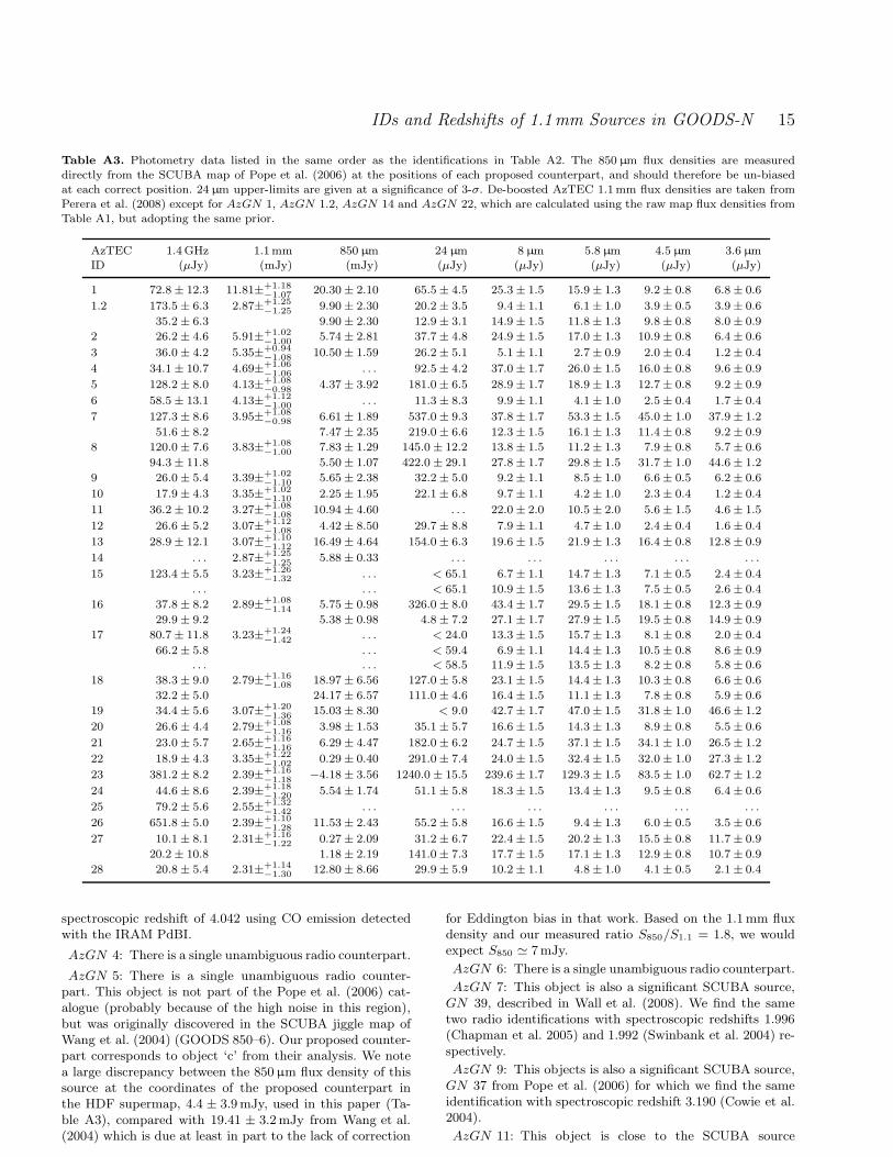
Table A2. Radio and Spitzer identifications of AzTEC sources (procedure described in Section 2). Counterpart distances in bracketsemployed a 10 arcsec search radius. P values in boldface emphasize robust counterparts with values < 0.05. Spectroscopic redshifts aregiven in the column labelled zspec (references for these measurements given in Appendix B). Photometric redshifts based on Spitzer IRflux densities from Table A3 are calculated using Equation 2 from Pope et al. (2006) and given in the penultimate column, zir. Theseredshifts have uncertainties ∆zir = 0.15(1+z), and are biased low at z > 3. Photometric redshifts based on the (sub)mm-to-radio colours
are given in the last column, zrm. The quoted 68 per cent uncertainties are theoretically derived; in this paper we assume an empiricallymeasured symmetric error ∆zrm = 0.8.
AzTEC SCUBA Radio Spitzer RedshiftID ID R.A. Dec. Dist. R.A. Dec. Dist. P zspec zir zrm
(h m s) (◦ ′ ′′) (′′) (h m s) (◦ ′ ′′) (′′)
1 20 12 37 11.88 +62 22 11.8 1.0 12 37 11.88 +62 22 12.1 1.3 0.003 4.055 2.7 3.8+1.2−0.7
1.2 20.2 12 37 08.78 +62 22 01.8 2.6 12 37 08.77 +62 22 01.8 2.7 0.005 4.052 2.5 3.1+1.2−0.2
12 37 09.73 +62 22 02.5 4.1 12 37 09.57 +62 22 02.1 2.9 0.037 . . . 3.1 2.5+0.8−0.8
2 . . . 12 36 31.93 +62 17 14.7 5.3 12 36 31.92 +62 17 14.6 5.2 0.051 . . . 3.2 2.4+2.3−0.1
3 10 12 36 33.42 +62 14 08.7 0.6 12 36 33.40 +62 14 08.4 0.6 0.002 4.042 2.3 3.1+1.4−0.2
4 . . . 12 35 50.26 +62 10 41.3 3.1 12 35 50.35 +62 10 41.8 2.7 0.030a . . . 2.9 2.4+2.2−0.2
5 . . . 12 37 30.78 +62 12 58.7 2.6 12 37 30.75 +62 12 58.4 2.2 0.007 . . . 2.0 2.1+1.6−0.9
6 . . . 12 36 27.26 +62 06 05.7 1.6 12 36 27.21 +62 06 05.7 1.2 0.007 . . . 3.0 2.9+1.4−1.1
7 39 12 37 11.32 +62 13 30.9 4.4 12 37 11.34 +62 13 31.0 4.3 0.014 1.996 1.7 2.7+0.9−0.8
12 37 11.99 +62 13 25.6 4.5 12 37 11.99 +62 13 25.7 4.4 0.032 1.992 2.0 >2.3
8 12 12 36 46.04 +62 14 48.6 (6.9) 12 36 46.07 +62 14 48.8 (7.0) 0.037 . . . 2.0 3.0+0.6−1.0
12 36 46.80 +62 14 45.3 (7.5) 12 36 46.88 +62 14 47.2 (9.0) 0.050 2.006 0.7 2.9+0.7−1.1
9 37 12 37 38.16 +62 17 37.0 1.6 12 37 38.26 +62 17 36.4 0.9 0.013 3.1900 2.4 >3.0
10 . . . 12 36 27.54 +62 12 17.8 3.5 12 36 27.48 +62 12 18.0 3.1 0.066a . . . 3.0 2.1+2.2−0.7
11 27 12 36 35.89 +62 07 03.8 3.1 0.027 . . . . . . 2.8+1.3−0.2
12 . . . 12 36 32.65 +62 06 21.1 4.7 12 36 32.65 +62 06 21.3 4.9 0.047 . . . 2.8 >1.3
13 . . . 12 35 54.23 +62 13 43.8 2.9 12 35 54.28 +62 13 43.4 3.3 0.033a . . . 2.2 2.6+0.9−1.5
c
14 14 12 36 52.07d +62 12 25.7d 1.2 . . . . . . . . .15 . . . 12 35 47.93 +62 15 29.2 5.0 12 35 48.09 +62 15 29.3 3.9 0.018 . . . . . . >1.6
12 35 47.87 +62 15 28.2 5.7 . . . . . . >1.6
16 04 12 36 16.09 +62 15 13.8 4.3 12 36 16.10 +62 15 13.6 4.5 0.038 2.578 2.0 2.4+2.1−0.2
12 36 15.80 +62 15 15.1 4.0 12 36 15.82 +62 15 15.4 3.6 0.039 . . . 4.5 3.0+0.3−0.2
17 . . . 12 35 39.92 +62 14 42.1 (7.6) 12 35 39.95 +62 14 40.8 (6.5) 0.062 . . . . . . >1.712 35 39.91 +62 14 30.8 (7.1) 12 35 39.97 +62 14 30.7 (6.9) 0.067 . . . . . . >1.7
12 35 39.76 +62 14 30.7 (7.9) . . . . . . >1.7
18 38 12 37 41.16 +62 12 20.5 3.8 12 37 41.16 +62 12 20.9 3.5 0.032 . . . 2.1 2.4+0.6−2.0
12 37 41.63 +62 12 23.6 5.8 12 37 41.66 +62 12 23.6 6.0 0.051 . . . 2.0 >2.2c
19 . . . 12 36 04.40 +62 07 02.7 2.6 12 36 04.43 +62 07 02.9 2.8 0.022 . . . . . . >1.520 . . . 12 37 12.48 +62 10 35.4 3.0 12 37 12.51 +62 10 35.6 2.8 0.030 . . . 3.3 >2.321 . . . 12 38 00.80 +62 16 11.7 1.5 12 38 00.81 +62 16 11.7 1.4 0.016a . . . 2.3 >1.622 . . . 12 36 48.60 +62 12 16.1 4.7 12 36 48.65 +62 12 15.7 4.2 0.083a . . . 1.7 >0.723 . . . 12 37 16.67 +62 17 33.2 1.4 12 37 16.67 +62 17 33.3 1.4 0.001 1.1460 1.6 >1.8
24 23 12 36 08.58 +62 14 35.3 (6.4) 12 36 08.60 +62 14 35.3 (6.4) 0.079 . . . 2.7 2.4+2.0−0.8
25 . . . 12 36 51.72 +62 05 03.0 4.1 0.021 . . . . . . >0.726 40 12 37 13.86 +62 18 26.2 0.6 12 37 13.85 +62 18 26.2 0.5 0.000 . . . 2.6 >0.727 . . . 12 37 19.62 +62 12 20.3 1.3 12 37 19.61 +62 12 20.9 0.9 0.034b . . . 3.1 >0.7
12 37 20.01 +62 12 22.0 2.1 12 37 19.99 +62 12 22.6 2.2 0.050b 2.4600 2.0 >0.728 . . . 12 36 44.03 +62 19 38.8 4.2 12 36 44.03 +62 19 38.4 3.9 0.071a . . . 2.5 >0.7
aIdentified in 3-σ radio cataloguebIdentified in MIPS 24 µm catalogue
cPhotometric redshift calculation excludes extremely noisy 850 µm photometrydPosition for HDF 850.1 from Dunlop et al. (2004). See also Cowie et al. (2009).
when only a single source was used, justifying the additionof the extra parameters. This procedure yields a clear 4.2-σ source which corresponds to GN 20.2 from Pope et al.(2006). There are two possible radio identifications, onefainter object is 4.1 arcsec away with P = 0.037, and theother brighter source is 2.6 arcsec away with P = 0.005. Thebrighter object is the claimed counterpart to AzGN 1.2 fromPope et al. (2006). However, both potential counterpartsmentioned here are also discussed in Daddi et al. (2008).
They detect a faint emission line from the brighter radiosource which they argue to be consistent with molecular COemission at a redshift 4.051. We concur with Daddi et al.(2008) that the brighter object is likely an AGN, based onits relatively large radio/mm flux ratio.
AzGN 3: The AzTEC detection, and proposed coun-terpart, are both coincident with the SCUBA sourceGN 10 and identification from Pope et al. (2006). Similarto AzGN 1 and AzGN 1.2, Daddi et al. (2009) identified a
IDs and Redshifts of 1.1mm Sources in GOODS-N 15
Table A3. Photometry data listed in the same order as the identifications in Table A2. The 850 µm flux densities are measureddirectly from the SCUBA map of Pope et al. (2006) at the positions of each proposed counterpart, and should therefore be un-biasedat each correct position. 24 µm upper-limits are given at a significance of 3-σ. De-boosted AzTEC 1.1mm flux densities are taken fromPerera et al. (2008) except for AzGN 1, AzGN 1.2, AzGN 14 and AzGN 22, which are calculated using the raw map flux densities fromTable A1, but adopting the same prior.
AzTEC 1.4GHz 1.1mm 850 µm 24 µm 8 µm 5.8 µm 4.5 µm 3.6 µmID (µJy) (mJy) (mJy) (µJy) (µJy) (µJy) (µJy) (µJy)
1 72.8 ± 12.3 11.81±+1.18−1.07 20.30 ± 2.10 65.5 ± 4.5 25.3 ± 1.5 15.9 ± 1.3 9.2 ± 0.8 6.8 ± 0.6
1.2 173.5 ± 6.3 2.87±+1.25−1.25
9.90 ± 2.30 20.2 ± 3.5 9.4 ± 1.1 6.1 ± 1.0 3.9 ± 0.5 3.9 ± 0.6
35.2 ± 6.3 9.90 ± 2.30 12.9 ± 3.1 14.9 ± 1.5 11.8 ± 1.3 9.8 ± 0.8 8.0 ± 0.9
2 26.2 ± 4.6 5.91±+1.02−1.00
5.74 ± 2.81 37.7 ± 4.8 24.9 ± 1.5 17.0 ± 1.3 10.9 ± 0.8 6.4 ± 0.6
3 36.0 ± 4.2 5.35±+0.94−1.08 10.50 ± 1.59 26.2 ± 5.1 5.1 ± 1.1 2.7 ± 0.9 2.0 ± 0.4 1.2 ± 0.4
4 34.1 ± 10.7 4.69±+1.06−1.06
. . . 92.5 ± 4.2 37.0 ± 1.7 26.0 ± 1.5 16.0 ± 0.8 9.6 ± 0.9
5 128.2 ± 8.0 4.13±+1.08−0.98
4.37 ± 3.92 181.0 ± 6.5 28.9 ± 1.7 18.9 ± 1.3 12.7 ± 0.8 9.2 ± 0.9
6 58.5 ± 13.1 4.13±+1.12−1.00 . . . 11.3 ± 8.3 9.9 ± 1.1 4.1 ± 1.0 2.5 ± 0.4 1.7 ± 0.4
7 127.3 ± 8.6 3.95±+1.08−0.98 6.61 ± 1.89 537.0 ± 9.3 37.8 ± 1.7 53.3 ± 1.5 45.0 ± 1.0 37.9 ± 1.2
51.6 ± 8.2 7.47 ± 2.35 219.0 ± 6.6 12.3 ± 1.5 16.1 ± 1.3 11.4 ± 0.8 9.2 ± 0.9
8 120.0 ± 7.6 3.83±+1.08−1.00
7.83 ± 1.29 145.0 ± 12.2 13.8 ± 1.5 11.2 ± 1.3 7.9 ± 0.8 5.7 ± 0.6
94.3 ± 11.8 5.50 ± 1.07 422.0 ± 29.1 27.8 ± 1.7 29.8 ± 1.5 31.7 ± 1.0 44.6 ± 1.2
9 26.0 ± 5.4 3.39±+1.02−1.10 5.65 ± 2.38 32.2 ± 5.0 9.2 ± 1.1 8.5 ± 1.0 6.6 ± 0.5 6.2 ± 0.6
10 17.9 ± 4.3 3.35±+1.02−1.10 2.25 ± 1.95 22.1 ± 6.8 9.7 ± 1.1 4.2 ± 1.0 2.3 ± 0.4 1.2 ± 0.4
11 36.2 ± 10.2 3.27±+1.08−1.08
10.94 ± 4.60 . . . 22.0 ± 2.0 10.5 ± 2.0 5.6 ± 1.5 4.6 ± 1.5
12 26.6 ± 5.2 3.07±+1.12−1.08 4.42 ± 8.50 29.7 ± 8.8 7.9 ± 1.1 4.7 ± 1.0 2.4 ± 0.4 1.6 ± 0.4
13 28.9 ± 12.1 3.07±+1.10−1.12 16.49 ± 4.64 154.0 ± 6.3 19.6 ± 1.5 21.9 ± 1.3 16.4 ± 0.8 12.8 ± 0.9
14 . . . 2.87±+1.25−1.25
5.88 ± 0.33 . . . . . . . . . . . . . . .
15 123.4 ± 5.5 3.23±+1.26−1.32 . . . < 65.1 6.7 ± 1.1 14.7 ± 1.3 7.1 ± 0.5 2.4 ± 0.4
. . . . . . < 65.1 10.9 ± 1.5 13.6 ± 1.3 7.5 ± 0.5 2.6 ± 0.4
16 37.8 ± 8.2 2.89±+1.08−1.14 5.75 ± 0.98 326.0 ± 8.0 43.4 ± 1.7 29.5 ± 1.5 18.1 ± 0.8 12.3 ± 0.9
29.9 ± 9.2 5.38 ± 0.98 4.8 ± 7.2 27.1 ± 1.7 27.9 ± 1.5 19.5 ± 0.8 14.9 ± 0.9
17 80.7 ± 11.8 3.23±+1.24−1.42
. . . < 24.0 13.3 ± 1.5 15.7 ± 1.3 8.1 ± 0.8 2.0 ± 0.4
66.2 ± 5.8 . . . < 59.4 6.9 ± 1.1 14.4 ± 1.3 10.5 ± 0.8 8.6 ± 0.9. . . . . . < 58.5 11.9 ± 1.5 13.5 ± 1.3 8.2 ± 0.8 5.8 ± 0.6
18 38.3 ± 9.0 2.79±+1.16−1.08 18.97 ± 6.56 127.0 ± 5.8 23.1 ± 1.5 14.4 ± 1.3 10.3 ± 0.8 6.6 ± 0.6
32.2 ± 5.0 24.17 ± 6.57 111.0 ± 4.6 16.4 ± 1.5 11.1 ± 1.3 7.8 ± 0.8 5.9 ± 0.6
19 34.4 ± 5.6 3.07±+1.20−1.36
15.03 ± 8.30 < 9.0 42.7 ± 1.7 47.0 ± 1.5 31.8 ± 1.0 46.6 ± 1.2
20 26.6 ± 4.4 2.79±+1.08−1.16
3.98 ± 1.53 35.1 ± 5.7 16.6 ± 1.5 14.3 ± 1.3 8.9 ± 0.8 5.5 ± 0.6
21 23.0 ± 5.7 2.65±+1.16−1.16 6.29 ± 4.47 182.0 ± 6.2 24.7 ± 1.5 37.1 ± 1.5 34.1 ± 1.0 26.5 ± 1.2
22 18.9 ± 4.3 3.35±+1.22−1.02 0.29 ± 0.40 291.0 ± 7.4 24.0 ± 1.5 32.4 ± 1.5 32.0 ± 1.0 27.3 ± 1.2
23 381.2 ± 8.2 2.39±+1.16−1.18
−4.18 ± 3.56 1240.0 ± 15.5 239.6 ± 1.7 129.3 ± 1.5 83.5 ± 1.0 62.7 ± 1.2
24 44.6 ± 8.6 2.39±+1.18−1.20 5.54 ± 1.74 51.1 ± 5.8 18.3 ± 1.5 13.4 ± 1.3 9.5 ± 0.8 6.4 ± 0.6
25 79.2 ± 5.6 2.55±+1.32−1.42 . . . . . . . . . . . . . . . . . .
26 651.8 ± 5.0 2.39±+1.10−1.28
11.53 ± 2.43 55.2 ± 5.8 16.6 ± 1.5 9.4 ± 1.3 6.0 ± 0.5 3.5 ± 0.6
27 10.1 ± 8.1 2.31±+1.16−1.22 0.27 ± 2.09 31.2 ± 6.7 22.4 ± 1.5 20.2 ± 1.3 15.5 ± 0.8 11.7 ± 0.9
20.2 ± 10.8 1.18 ± 2.19 141.0 ± 7.3 17.7 ± 1.5 17.1 ± 1.3 12.9 ± 0.8 10.7 ± 0.9
28 20.8 ± 5.4 2.31±+1.14−1.30 12.80 ± 8.66 29.9 ± 5.9 10.2 ± 1.1 4.8 ± 1.0 4.1 ± 0.5 2.1 ± 0.4
spectroscopic redshift of 4.042 using CO emission detectedwith the IRAM PdBI.
AzGN 4: There is a single unambiguous radio counterpart.
AzGN 5: There is a single unambiguous radio counter-part. This object is not part of the Pope et al. (2006) cat-alogue (probably because of the high noise in this region),but was originally discovered in the SCUBA jiggle map ofWang et al. (2004) (GOODS 850–6). Our proposed counter-part corresponds to object ‘c’ from their analysis. We notea large discrepancy between the 850 µm flux density of thissource at the coordinates of the proposed counterpart inthe HDF supermap, 4.4 ± 3.9 mJy, used in this paper (Ta-ble A3), compared with 19.41 ± 3.2 mJy from Wang et al.(2004) which is due at least in part to the lack of correction
for Eddington bias in that work. Based on the 1.1 mm fluxdensity and our measured ratio S850/S1.1 = 1.8, we wouldexpect S850 ≃ 7mJy.
AzGN 6: There is a single unambiguous radio counterpart.
AzGN 7: This object is also a significant SCUBA source,GN 39, described in Wall et al. (2008). We find the sametwo radio identifications with spectroscopic redshifts 1.996(Chapman et al. 2005) and 1.992 (Swinbank et al. 2004) re-spectively.
AzGN 9: This objects is also a significant SCUBA source,GN 37 from Pope et al. (2006) for which we find the sameidentification with spectroscopic redshift 3.190 (Cowie et al.2004).
AzGN 11: This object is close to the SCUBA source
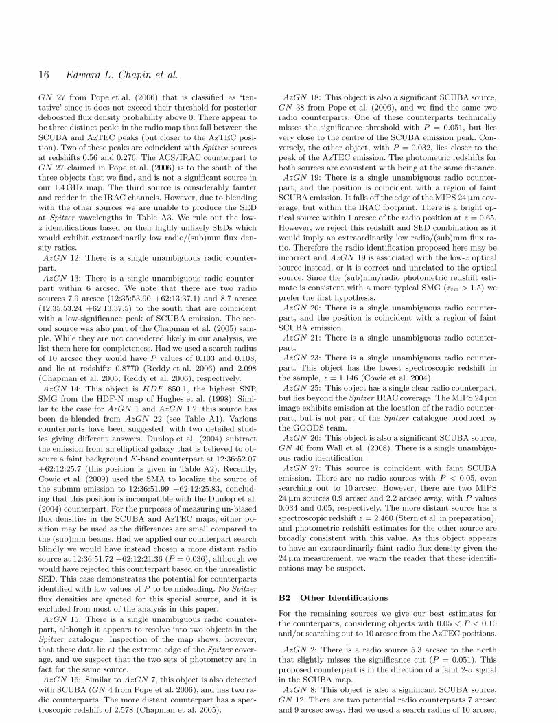
16 Edward L. Chapin et al.
GN 27 from Pope et al. (2006) that is classified as ‘ten-tative’ since it does not exceed their threshold for posteriordeboosted flux density probability above 0. There appear tobe three distinct peaks in the radio map that fall between theSCUBA and AzTEC peaks (but closer to the AzTEC posi-tion). Two of these peaks are coincident with Spitzer sourcesat redshifts 0.56 and 0.276. The ACS/IRAC counterpart toGN 27 claimed in Pope et al. (2006) is to the south of thethree objects that we find, and is not a significant source inour 1.4 GHz map. The third source is considerably fainterand redder in the IRAC channels. However, due to blendingwith the other sources we are unable to produce the SEDat Spitzer wavelengths in Table A3. We rule out the low-z identifications based on their highly unlikely SEDs whichwould exhibit extraordinarily low radio/(sub)mm flux den-sity ratios.
AzGN 12: There is a single unambiguous radio counter-part.
AzGN 13: There is a single unambiguous radio counter-part within 6 arcsec. We note that there are two radiosources 7.9 arcsec (12:35:53.90 +62:13:37.1) and 8.7 arcsec(12:35:53.24 +62:13:37.5) to the south that are coincidentwith a low-significance peak of SCUBA emission. The sec-ond source was also part of the Chapman et al. (2005) sam-ple. While they are not considered likely in our analysis, welist them here for completeness. Had we used a search radiusof 10 arcsec they would have P values of 0.103 and 0.108,and lie at redshifts 0.8770 (Reddy et al. 2006) and 2.098(Chapman et al. 2005; Reddy et al. 2006), respectively.
AzGN 14: This object is HDF 850.1, the highest SNRSMG from the HDF-N map of Hughes et al. (1998). Simi-lar to the case for AzGN 1 and AzGN 1.2, this source hasbeen de-blended from AzGN 22 (see Table A1). Variouscounterparts have been suggested, with two detailed stud-ies giving different answers. Dunlop et al. (2004) subtractthe emission from an elliptical galaxy that is believed to ob-scure a faint background K-band counterpart at 12:36:52.07+62:12:25.7 (this position is given in Table A2). Recently,Cowie et al. (2009) used the SMA to localize the source ofthe submm emission to 12:36:51.99 +62:12:25.83, conclud-ing that this position is incompatible with the Dunlop et al.(2004) counterpart. For the purposes of measuring un-biasedflux densities in the SCUBA and AzTEC maps, either po-sition may be used as the differences are small compared tothe (sub)mm beams. Had we applied our counterpart searchblindly we would have instead chosen a more distant radiosource at 12:36:51.72 +62:12:21.36 (P = 0.036), although wewould have rejected this counterpart based on the unrealisticSED. This case demonstrates the potential for counterpartsidentified with low values of P to be misleading. No Spitzer
flux densities are quoted for this special source, and it isexcluded from most of the analysis in this paper.
AzGN 15: There is a single unambiguous radio counter-part, although it appears to resolve into two objects in theSpitzer catalogue. Inspection of the map shows, however,that these data lie at the extreme edge of the Spitzer cover-age, and we suspect that the two sets of photometry are infact for the same source.
AzGN 16: Similar to AzGN 7, this object is also detectedwith SCUBA (GN 4 from Pope et al. 2006), and has two ra-dio counterparts. The more distant counterpart has a spec-troscopic redshift of 2.578 (Chapman et al. 2005).
AzGN 18: This object is also a significant SCUBA source,GN 38 from Pope et al. (2006), and we find the same tworadio counterparts. One of these counterparts technicallymisses the significance threshold with P = 0.051, but liesvery close to the centre of the SCUBA emission peak. Con-versely, the other object, with P = 0.032, lies closer to thepeak of the AzTEC emission. The photometric redshifts forboth sources are consistent with being at the same distance.AzGN 19: There is a single unambiguous radio counter-
part, and the position is coincident with a region of faintSCUBA emission. It falls off the edge of the MIPS 24 µm cov-erage, but within the IRAC footprint. There is a bright op-tical source within 1 arcsec of the radio position at z = 0.65.However, we reject this redshift and SED combination as itwould imply an extraordinarily low radio/(sub)mm flux ra-tio. Therefore the radio identification proposed here may beincorrect and AzGN 19 is associated with the low-z opticalsource instead, or it is correct and unrelated to the opticalsource. Since the (sub)mm/radio photometric redshift esti-mate is consistent with a more typical SMG (zrm > 1.5) weprefer the first hypothesis.AzGN 20: There is a single unambiguous radio counter-
part, and the position is coincident with a region of faintSCUBA emission.AzGN 21: There is a single unambiguous radio counter-
part.AzGN 23: There is a single unambiguous radio counter-
part. This object has the lowest spectroscopic redshift inthe sample, z = 1.146 (Cowie et al. 2004).AzGN 25: This object has a single clear radio counterpart,
but lies beyond the Spitzer IRAC coverage. The MIPS 24 µmimage exhibits emission at the location of the radio counter-part, but is not part of the Spitzer catalogue produced bythe GOODS team.AzGN 26: This object is also a significant SCUBA source,
GN 40 from Wall et al. (2008). There is a single unambigu-ous radio identification.AzGN 27: This source is coincident with faint SCUBA
emission. There are no radio sources with P < 0.05, evensearching out to 10 arcsec. However, there are two MIPS24µm sources 0.9 arcsec and 2.2 arcsec away, with P values0.034 and 0.05, respectively. The more distant source has aspectroscopic redshift z = 2.460 (Stern et al. in preparation),and photometric redshift estimates for the other source arebroadly consistent with this value. As this object appearsto have an extraordinarily faint radio flux density given the24µm measurement, we warn the reader that these identifi-cations may be suspect.
B2 Other Identifications
For the remaining sources we give our best estimates forthe counterparts, considering objects with 0.05 < P < 0.10and/or searching out to 10 arcsec from the AzTEC positions.
AzGN 2: There is a radio source 5.3 arcsec to the norththat slightly misses the significance cut (P = 0.051). Thisproposed counterpart is in the direction of a faint 2-σ signalin the SCUBA map.AzGN 8: This object is also a significant SCUBA source,
GN 12. There are two potential radio counterparts 7 arcsecand 9 arcsec away. Had we used a search radius of 10 arcsec,
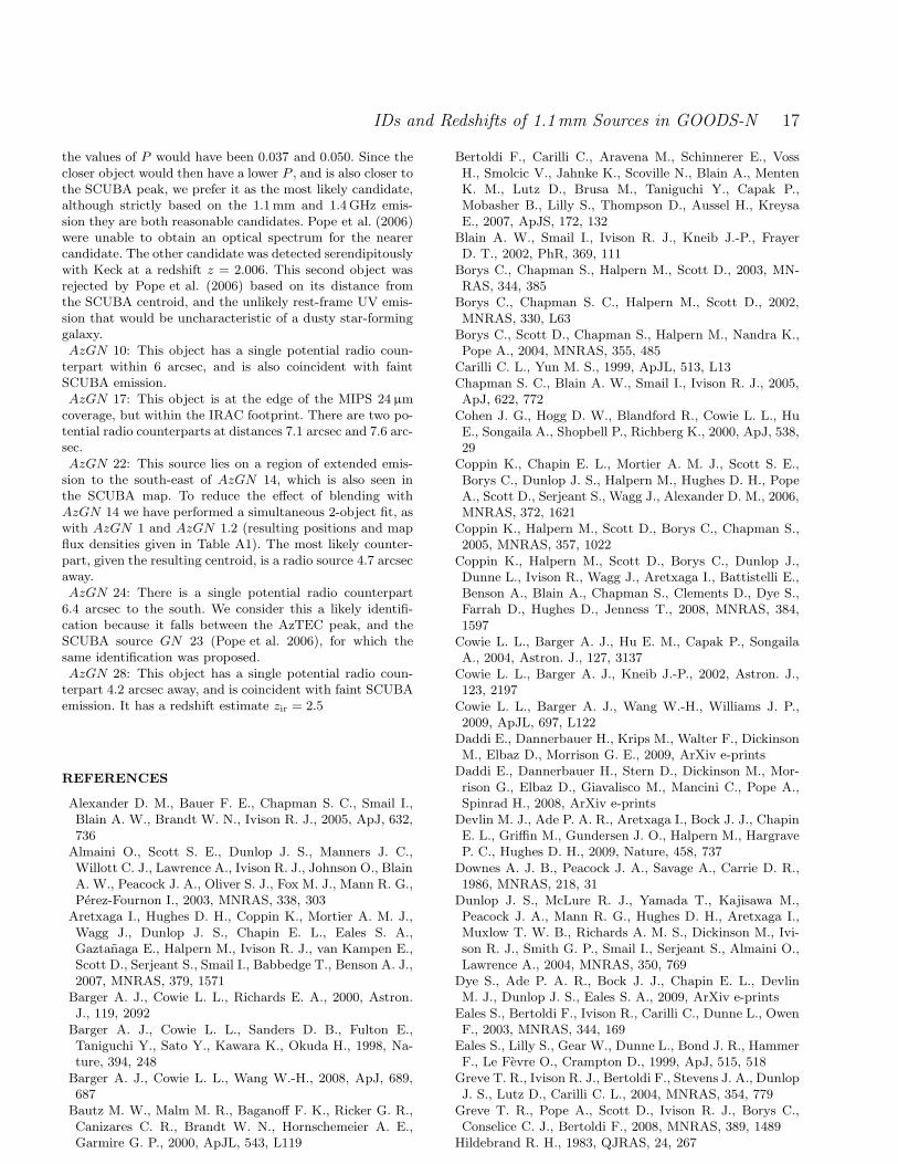
IDs and Redshifts of 1.1mm Sources in GOODS-N 17
the values of P would have been 0.037 and 0.050. Since thecloser object would then have a lower P , and is also closer tothe SCUBA peak, we prefer it as the most likely candidate,although strictly based on the 1.1 mm and 1.4 GHz emis-sion they are both reasonable candidates. Pope et al. (2006)were unable to obtain an optical spectrum for the nearercandidate. The other candidate was detected serendipitouslywith Keck at a redshift z = 2.006. This second object wasrejected by Pope et al. (2006) based on its distance fromthe SCUBA centroid, and the unlikely rest-frame UV emis-sion that would be uncharacteristic of a dusty star-forminggalaxy.AzGN 10: This object has a single potential radio coun-
terpart within 6 arcsec, and is also coincident with faintSCUBA emission.AzGN 17: This object is at the edge of the MIPS 24 µm
coverage, but within the IRAC footprint. There are two po-tential radio counterparts at distances 7.1 arcsec and 7.6 arc-sec.AzGN 22: This source lies on a region of extended emis-
sion to the south-east of AzGN 14, which is also seen inthe SCUBA map. To reduce the effect of blending withAzGN 14 we have performed a simultaneous 2-object fit, aswith AzGN 1 and AzGN 1.2 (resulting positions and mapflux densities given in Table A1). The most likely counter-part, given the resulting centroid, is a radio source 4.7 arcsecaway.AzGN 24: There is a single potential radio counterpart
6.4 arcsec to the south. We consider this a likely identifi-cation because it falls between the AzTEC peak, and theSCUBA source GN 23 (Pope et al. 2006), for which thesame identification was proposed.AzGN 28: This object has a single potential radio coun-
terpart 4.2 arcsec away, and is coincident with faint SCUBAemission. It has a redshift estimate zir = 2.5
REFERENCES
Alexander D. M., Bauer F. E., Chapman S. C., Smail I.,Blain A. W., Brandt W. N., Ivison R. J., 2005, ApJ, 632,736
Almaini O., Scott S. E., Dunlop J. S., Manners J. C.,Willott C. J., Lawrence A., Ivison R. J., Johnson O., BlainA. W., Peacock J. A., Oliver S. J., Fox M. J., Mann R. G.,Perez-Fournon I., 2003, MNRAS, 338, 303
Aretxaga I., Hughes D. H., Coppin K., Mortier A. M. J.,Wagg J., Dunlop J. S., Chapin E. L., Eales S. A.,Gaztanaga E., Halpern M., Ivison R. J., van Kampen E.,Scott D., Serjeant S., Smail I., Babbedge T., Benson A. J.,2007, MNRAS, 379, 1571
Barger A. J., Cowie L. L., Richards E. A., 2000, Astron.J., 119, 2092
Barger A. J., Cowie L. L., Sanders D. B., Fulton E.,Taniguchi Y., Sato Y., Kawara K., Okuda H., 1998, Na-ture, 394, 248
Barger A. J., Cowie L. L., Wang W.-H., 2008, ApJ, 689,687
Bautz M. W., Malm M. R., Baganoff F. K., Ricker G. R.,Canizares C. R., Brandt W. N., Hornschemeier A. E.,Garmire G. P., 2000, ApJL, 543, L119
Bertoldi F., Carilli C., Aravena M., Schinnerer E., VossH., Smolcic V., Jahnke K., Scoville N., Blain A., MentenK. M., Lutz D., Brusa M., Taniguchi Y., Capak P.,Mobasher B., Lilly S., Thompson D., Aussel H., KreysaE., 2007, ApJS, 172, 132
Blain A. W., Smail I., Ivison R. J., Kneib J.-P., FrayerD. T., 2002, PhR, 369, 111
Borys C., Chapman S., Halpern M., Scott D., 2003, MN-RAS, 344, 385
Borys C., Chapman S. C., Halpern M., Scott D., 2002,MNRAS, 330, L63
Borys C., Scott D., Chapman S., Halpern M., Nandra K.,Pope A., 2004, MNRAS, 355, 485
Carilli C. L., Yun M. S., 1999, ApJL, 513, L13Chapman S. C., Blain A. W., Smail I., Ivison R. J., 2005,ApJ, 622, 772
Cohen J. G., Hogg D. W., Blandford R., Cowie L. L., HuE., Songaila A., Shopbell P., Richberg K., 2000, ApJ, 538,29
Coppin K., Chapin E. L., Mortier A. M. J., Scott S. E.,Borys C., Dunlop J. S., Halpern M., Hughes D. H., PopeA., Scott D., Serjeant S., Wagg J., Alexander D. M., 2006,MNRAS, 372, 1621
Coppin K., Halpern M., Scott D., Borys C., Chapman S.,2005, MNRAS, 357, 1022
Coppin K., Halpern M., Scott D., Borys C., Dunlop J.,Dunne L., Ivison R., Wagg J., Aretxaga I., Battistelli E.,Benson A., Blain A., Chapman S., Clements D., Dye S.,Farrah D., Hughes D., Jenness T., 2008, MNRAS, 384,1597
Cowie L. L., Barger A. J., Hu E. M., Capak P., SongailaA., 2004, Astron. J., 127, 3137
Cowie L. L., Barger A. J., Kneib J.-P., 2002, Astron. J.,123, 2197
Cowie L. L., Barger A. J., Wang W.-H., Williams J. P.,2009, ApJL, 697, L122
Daddi E., Dannerbauer H., Krips M., Walter F., DickinsonM., Elbaz D., Morrison G. E., 2009, ArXiv e-prints
Daddi E., Dannerbauer H., Stern D., Dickinson M., Mor-rison G., Elbaz D., Giavalisco M., Mancini C., Pope A.,Spinrad H., 2008, ArXiv e-prints
Devlin M. J., Ade P. A. R., Aretxaga I., Bock J. J., ChapinE. L., Griffin M., Gundersen J. O., Halpern M., HargraveP. C., Hughes D. H., 2009, Nature, 458, 737
Downes A. J. B., Peacock J. A., Savage A., Carrie D. R.,1986, MNRAS, 218, 31
Dunlop J. S., McLure R. J., Yamada T., Kajisawa M.,Peacock J. A., Mann R. G., Hughes D. H., Aretxaga I.,Muxlow T. W. B., Richards A. M. S., Dickinson M., Ivi-son R. J., Smith G. P., Smail I., Serjeant S., Almaini O.,Lawrence A., 2004, MNRAS, 350, 769
Dye S., Ade P. A. R., Bock J. J., Chapin E. L., DevlinM. J., Dunlop J. S., Eales S. A., 2009, ArXiv e-prints
Eales S., Bertoldi F., Ivison R., Carilli C., Dunne L., OwenF., 2003, MNRAS, 344, 169
Eales S., Lilly S., Gear W., Dunne L., Bond J. R., HammerF., Le Fevre O., Crampton D., 1999, ApJ, 515, 518
Greve T. R., Ivison R. J., Bertoldi F., Stevens J. A., DunlopJ. S., Lutz D., Carilli C. L., 2004, MNRAS, 354, 779
Greve T. R., Pope A., Scott D., Ivison R. J., Borys C.,Conselice C. J., Bertoldi F., 2008, MNRAS, 389, 1489
Hildebrand R. H., 1983, QJRAS, 24, 267
18 Edward L. Chapin et al.
Hornschemeier A. E., Brandt W. N., Garmire G. P., Schnei-der D. P., Broos P. S., Townsley L. K., Bautz M. W.,Burrows D. N., Chartas G., Feigelson E. D., Griffiths R.,Lumb D., Nousek J. A., Sargent W. L. W., 2000, ApJ,541, 49
Hughes D. H., Serjeant S., Dunlop J., Rowan-Robinson M.,Blain A., Mann R. G., Ivison R., Peacock J., EfstathiouA., Gear W., Oliver S., Lawrence A., Longair M., Gold-schmidt P., Jenness T., 1998, Nature, 394, 241
Huynh M. T., Pope A., Frayer D. T., Scott D., 2007, ApJ,659, 305
Iono D., Peck A. B., Pope A., Borys C., Scott D., WilnerD. J., Gurwell M., Ho P. T. P., Yun M. S., MatsushitaS., Petitpas G. R., Dunlop J. S., Elvis M., Blain A., LeFloc’h E., 2006, ApJL, 640, L1
Ivison R. J., Greve T. R., Dunlop J. S., Peacock J. A.,Egami E., Smail I., Ibar E., van Kampen E., Aretxaga I.,Babbedge T., Biggs A. D., Blain A. W., Chapman S. C.,Clements D. L., 2007, MNRAS, 380, 199
Ivison R. J., Greve T. R., Smail I., Dunlop J. S., RocheN. D., Scott S. E., Page M. J., Stevens J. A., AlmainiO., Blain A. W., Willott C. J., Fox M. J., Gilbank D. G.,Serjeant S., Hughes D. H., 2002, MNRAS, 337, 1
Khan S. A., Shafer R. A., Serjeant S., Willner S. P., PearsonC. P., Benford D. J., Staguhn J. G., Moseley S. H., SumnerT. J., Ashby M. L. N., Borys C. K., Chanial P., ClementsD. L., Dowell C. D., Dwek E., Fazio G. G., Kovacs A., LeFloc’h E., Silverberg R. F., 2007, ApJ, 665, 973
Knudsen K. K., Barnard V. E., van der Werf P. P., VielvaP., Kneib J.-P., Blain A. W., Barreiro R. B., Ivison R. J.,Smail I., Peacock J. A., 2006, MNRAS, 368, 487
Kovacs A., Chapman S. C., Dowell C. D., Blain A. W.,Ivison R. J., Smail I., Phillips T. G., 2006, ApJ, 650, 592
Laurent G. T., Aguirre J. E., Glenn J., Ade P. A. R., BockJ. J., Edgington S. F., Goldin A., Golwala S. R., Haig D.,Lange A. E., Maloney P. R., Mauskopf P. D., Nguyen H.,Rossinot P., Sayers J., Stover P., 2005, ApJ, 623, 742
Magnelli B., Elbaz D., Chary R. R., Dickinson M., LeBorgne D., Frayer D. T., Willmer C. N. A., 2009, A&A,496, 57
Perera T. A., Chapin E. L., Austermann J. E., Scott K. S.,Wilson G. W., Halpern M., Pope A., Scott D., Yun M. S.,Lowenthal J. D., Morrison G., Aretxaga I., Bock J. J.,Coppin K., Crowe M., Frey L., Hughes D. H., Kang Y.,Kim S., Mauskopf P. D., 2008, ArXiv e-prints, 806
Pope A., Borys C., Scott D., Conselice C., Dickinson M.,Mobasher B., 2005, MNRAS, 358, 149
Pope A., Chary R.-R., Alexander D. M., Armus L., Dick-inson M., Elbaz D., Frayer D., Scott D., Teplitz H., 2008,ApJ, 675, 1171
Pope A., Scott D., Dickinson M., Chary R.-R., Morrison G.,Borys C., Sajina A., Alexander D. M., Daddi E., FrayerD., MacDonald E., Stern D., 2006, MNRAS, 370, 1185
Reddy N. A., Steidel C. C., Erb D. K., Shapley A. E.,Pettini M., 2006, ApJ, 653, 1004
Richards E. A., 2000, ApJ, 533, 611Sanders D. B., Mirabel I. F., 1996, ARAA, 34, 749Sawicki M., 2002, Astron. J., 124, 3050Scott K. S., Austermann J. E., Perera T. A., Wilson G. W.,Aretxaga I., Bock J. J., Hughes D. H., Kang Y., Kim S.,Mauskopf P. D., Sanders D. B., Scoville N., Yun M. S.,2008, MNRAS, 385, 2225
Scott S. E., Fox M. J., Dunlop J. S., Serjeant S., Pea-cock J. A., Ivison R. J., Oliver S., Mann R. G., LawrenceA., Efstathiou A., Rowan-Robinson M., Hughes D. H.,Archibald E. N., Blain A., Longair M., 2002, MNRAS,331, 817
Serjeant S., Dunlop J. S., Mann R. G., Rowan-RobinsonM., Hughes D., Efstathiou A., Blain A., Fox M., IvisonR. J., Jenness T., Lawrence A., Longair M., Oliver S.,Peacock J. A., 2003, MNRAS, 344, 887
Simpson C., Eisenhardt P., 1999, PASP, 111, 691Smail I., Ivison R. J., Blain A. W., 1997, ApJL, 490, L5+Smail I., Ivison R. J., Blain A. W., Kneib J.-P., 2002, MN-RAS, 331, 495
Swinbank A. M., Smail I., Chapman S. C., Blain A. W.,Ivison R. J., Keel W. C., 2004, ApJ, 617, 64
Wall J. V., Pope A., Scott D., 2008, MNRAS, 383, 435Wang W.-H., Cowie L. L., Barger A. J., 2004, ApJ, 613,655
Webb T. M., Eales S. A., Lilly S. J., Clements D. L., DunneL., Gear W. K., Ivison R. J., Flores H., Yun M., 2003, ApJ,587, 41
Wilson G. W., Austermann J. E., Perera T. A., Scott K. S.,Ade P. A. R., Bock J. J., Glenn J., Golwala S. R., KimS., Kang Y., Lydon D., Mauskopf P. D., Predmore C. R.,Roberts C. M., Souccar K., Yun M. S., 2008, MNRAS,386, 807
Wilson G. W., Hughes D. H., Aretxaga I., Ezawa H.,Austermann J. E., Doyle S., Ferrusca D., 2008, MNRAS,390, 1061
Wirth G. D., Willmer C. N. A., Amico P., Chaffee F. H.,Goodrich R. W., Kwok S., Lyke J. E., Mader J. A., TranH. D., Barger A. J., Cowie L. L., Capak P., Coil A. L.,Cooper M. C., 2004, Astron. J., 127, 3121
Younger J. D., Fazio G. G., Huang J.-S., Yun M. S., WilsonG. W., Ashby M. L. N., Gurwell M. A., Lai K., Peck A. B.,Petitpas G. R., Wilner D. J., Iono D., Kohno K., KawabeR., Hughes D. H., Aretxaga I., Webb T., 2007, ApJ, 671,1531
Yun M. S., Aretxaga I., Ashby M. L. N., Austermann J.,Fazio G. G., Giavalisco M., Huang J.-S., Hughes D. H.,Kim S., Lowenthal J. D., Perera T., Scott K., Wilson G.,Younger J. D., 2008, MNRAS, 389, 333