An automated prognosis system for estrogen hormone status assessment in breast cancer tissue samples

Turk J Elec Eng & Comp Sci

(2013) 21: 1199 – 1221

c© TUBITAK

doi:10.3906/elk-1111-10

Turkish Journal of Electrical Engineering & Computer Sciences

http :// journa l s . tub i tak .gov . t r/e lektr ik/

Research Article

An automated prognosis system for estrogen hormone status assessment in breast

cancer tissue samples

Fatih SARIKOC,1 Adem KALINLI,1,∗ Hulya AKGUN,2 Figen OZTURK2

1Department of Computer Engineering, Faculty of Engineering, Erciyes University, 38039 Kayseri, Turkey2Department of Pathology, Faculty of Medicine, Erciyes University, 38039 Kayseri, Turkey

Received: 03.11.2011 • Accepted: 17.02.2012 • Published Online: 03.06.2013 • Printed: 24.06.2013

Abstract: Estrogen receptor (ER) status evaluation is a widely applied method in the prognosis of breast cancer.

However, testing for the existence of the ER biomarker in a patient’s tumor sample mainly depends on the subjective

decisions of the doctors. The aim of this paper is to introduce the usage of a machine learning tool, functional trees

(FTs), to attain an ER prognosis of the disease via an objective decision model. For this aim, 27 image files, each of which

came from a biopsy sample of an invasive ductal carcinoma patient, were scanned and captured by a light microscope.

From these images, 5150 nuclei were segmented with image processing methods. Several attributes, including statistical,

wavelet, cooccurrence matrix, and Laws’ texture features, were calculated inside the border area of each nucleus. A FT

was trained over the feature dataset using a 10-fold cross-validation and then the obtained model was tested on a separate

dataset. The assessment results of the model were compared with those of 2 experts. Consequently, the weighted kappa

coefficient indicated a very good agreement (κ = 0.899 and κ = 0.927, P < 0.001) and the Spearman’s rank order

correlation showed a high level of correlation (ρ = 0.963 and ρ = 0.943, P < 0.001) between the results of the FT and

those of the observers. The Wilcoxon test revealed that there was no significant difference between the results of the

experts and the model (P = 0.051 and P = 0.316). Finally, it was concluded from the results that the FT could be used

as a tool to support the decision of doctors by indicating consistent outputs and hence contribute to the objectiveness

and reproducibility of the assessment results.

Key words: Image processing, nucleus classification, segmentation, functional trees, estrogen receptor status evaluation,

breast cancer prognosis, Allred scoring, machine learning

1. Introduction

Breast cancer is the second most frequently diagnosed cancer type among the female population of industrializedcountries. For patients who have a cancer diagnosis, the treatment type, duration, cost, effective chemicalsubstance, and survival are decided upon based on the prognosis results. One of the important prognosticfactors of this disease is the evaluation of the hormone receptor presence in the tumor section [1,2].

Immunohistochemical (IHC) staining of a sample biopsy section is a common method to assess the

presence of an estrogen receptor (ER), since it provides cheap material and is an easy procedure [3]. In thisstudy, a computer-based assessment of the ER status was introduced according to the Allred scoring system,where several scoring alternatives are available in medical practice [4–6]. This scoring system is easy to use and

is able to identify low-positive cases [7,8] to avoid having false-negative results.

∗Correspondence: [email protected]

1199

SARIKOC et al./Turk J Elec Eng & Comp Sci

Despite its widespread usage for prognosis, the assessment of the ER is done subjectively, relying upon theperception of the observer. Due to physiopsychological variation in the perception of human vision, an observermay give different score values for the same specimen at different times (intraobserver variation) or different

observers may give different score values for the same specimen at the same time (interobserver variation).

Interpretation subjectivity of observers was reported in [9]. This study included 172 pathologists in Germany,

revealing that 24% of the pathologists’ ER interpretations were in fact false negatives. Having false negativeswill lead to the consequence that these patients will be labeled as ER-negative and will not receive the benefitof endocrine therapy.

According to a survey about IHC techniques, interpretation variation may come from different laboratoryconditions and the diversity of IHC staining procedures, such as the duration of the tissue fixation, typeof antigen retrieval, antibody specificity, and dilution or detection systems [5]. Therefore, IHC results lack

standardization and reproducibility [10]. Even though different conditions are maintained in the same base, itwould not be possible to reach standardization and reproducibility of IHC results unless the interobserver andintraobserver variation of the human factor is overcome or at least minimized. With this motivation in mind,aside from searching for standard procedures in different laboratory conditions, several computer-aided systemsand methods have also been presented up to now.

Some of the methods implement global thresholding techniques by the intensity or optical density valuesof several color spaces [10–22]. Some works focus on texture and morphological features [23–25]. Recently,Krecsak et al. introduced NuclearQuant software, which benefits from color, intensity, and size features fornuclei detection [26]. Tuominen et al. introduced a web-based software for nuclei quantification relying on an

image color deconvolution algorithm [27]. In this paper, we use color and gray-level statistical, textural, andspectral features while comparing the classification performance of each feature set separately.

When the literature is searched for ER status evaluation, there are several machine learning methodsused in this area of medical implementation. These are k-nearest neighbors with weighted votes [23], radial basis

neural networks [24], k-means clustering [25], random forest clustering [28], and probabilistic neural network

and support vector machines [29]. These papers refer to different scoring protocols than the one that we used.

There is not a unique scoring protocol that is used as a reference for all of the methods. Calculatingthe agreement or correlation coefficient over a 3- or 8-range scoring protocol might yield different performanceresults. For this reason, it is not directly possible to compare the achievements of all of the approaches. However,in a survey in [7], it was affirmed that the Allred scoring protocol is becoming widely accepted in medicallaboratories because of its low-level scoring sensitivity with additional scoring ranges and the considerationof intensity variation in staining. Hence, the Allred scoring protocol was implemented as a reference scoringprotocol in our work.

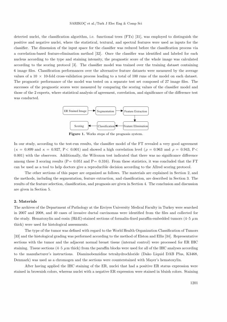
We designed a computer-based approach in which several work steps depicted in Figure 1 were automat-ically realized without user interaction. First, an expert captured a representative region of the ER-stainedspecimen with a light microscope and recorded the vision as an image file. After that, the work of automatedanalysis started. In the image file, the stained nuclei were segmented from the other structures of the back-ground tissue. This process was carried out by use of the Otsu thresholding method [30], benefiting from thefact that positive- or negative-stained nuclei have a darker appearance compared to the cytoplasm and otherparts of the tissue. However, there were some components such as the stromal cells that looked very similarto the nuclei stain. Those types of components were eliminated with morphological operators, as their sizeswere obviously smaller than that of the nuclei. Having obtained a segmented image file that only showed the

1200


detected nuclei, the classification algorithm, i.e. functional trees (FTs) [31], was employed to distinguish thepositive and negative nuclei, where the statistical, textural, and spectral features were used as inputs for theclassifier. The dimension of the input space for the classifier was reduced before the classification process viaa correlation-based feature-elimination method [32]. Once the classifier was identified and labeled for eachnucleus according to the type and staining intensity, the prognostic score of the whole image was calculatedaccording to the scoring protocol [3]. The classifier model was trained over the training dataset containing6 image files. Classification performances over the alternative feature datasets were measured by the averagevalues of a 10 × 10-fold cross-validation process leading to a total of 100 runs of the model on each dataset.The prognostic performance of the model was tested on a separate test set composed of 27 image files. Thesuccesses of the prognostic scores were measured by comparing the scoring values of the classifier model andthose of the 2 experts, where statistical analysis of agreement, correlation, and significance of the difference testwas conducted.

ER Stained Image Segmentation Feature Extraction

Feature EliminationScoring Classification

Figure 1. Works steps of the prognosis system.

In our study, according to the test-run results, the classifier model of the FT revealed a very good agreement(κ = 0.899 and κ = 0.927, P< 0.001) and showed a high correlation level (ρ = 0.963 and ρ = 0.943, P<

0.001) with the observers. Additionally, the Wilcoxon test indicated that there was no significance difference

among these 3 scoring results (P= 0.051 and P= 0.316). From these statistics, it was concluded that the FTcan be used as a tool to help doctors give a reproducible decision according to the Allred scoring protocol.

The other sections of this paper are organized as follows. The materials are explained in Section 2, andthe methods, including the segmentation, feature extraction, and classification, are described in Section 3. Theresults of the feature selection, classification, and prognosis are given in Section 4. The conclusion and discussionare given in Section 5.

2. Materials

The archives of the Department of Pathology at the Erciyes University Medical Faculty in Turkey were searchedin 2007 and 2008, and 40 cases of invasive ductal carcinomas were identified from the files and collected forthe study. Hematoxylin and eosin (H&E)-stained sections of formalin-fixed paraffin-embedded tumors (4–5 μm

thick) were used for histological assessments.

The type of the tumor was defined with regard to the World Health Organization Classification of Tumors[33] and the histological grading was performed according to the method of Elston and Ellis [34]. Representative

sections with the tumor and the adjacent normal breast tissue (internal control) were processed for ER IHC

staining. Tissue sections (4–5 μm thick) from the paraffin blocks were used for all of the IHC analyses according

to the manufacturer’s instructions. Diaminobenzidine tetrahydrochloride (Dako Liquid DAB Plus, K3468,

Denmark) was used as a chromogen and the sections were counterstained with Mayer’s hematoxylin.

After having applied the IHC staining of the ER, nuclei that had a positive ER status expression werestained in brownish colors, whereas nuclei with a negative ER expression were stained in bluish colors. Staining

1201


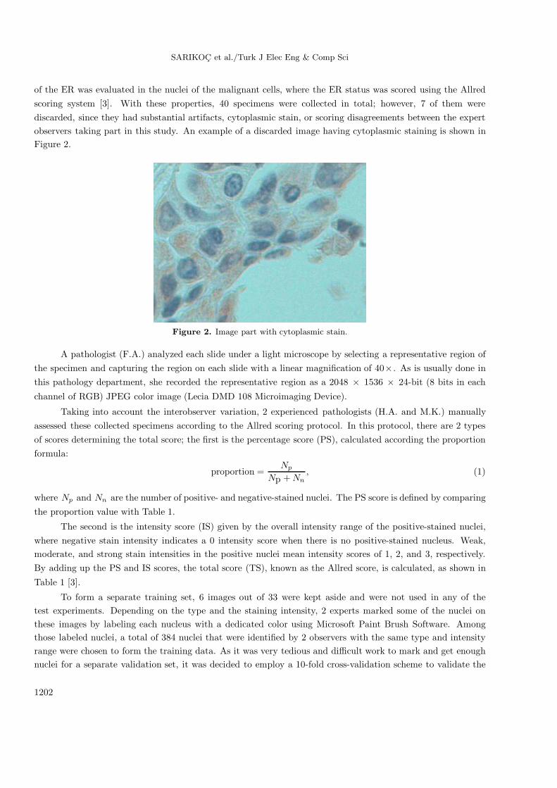
of the ER was evaluated in the nuclei of the malignant cells, where the ER status was scored using the Allredscoring system [3]. With these properties, 40 specimens were collected in total; however, 7 of them werediscarded, since they had substantial artifacts, cytoplasmic stain, or scoring disagreements between the expertobservers taking part in this study. An example of a discarded image having cytoplasmic staining is shown inFigure 2.

Figure 2. Image part with cytoplasmic stain.

A pathologist (F.A.) analyzed each slide under a light microscope by selecting a representative region ofthe specimen and capturing the region on each slide with a linear magnification of 40× . As is usually done inthis pathology department, she recorded the representative region as a 2048 × 1536 × 24-bit (8 bits in each

channel of RGB) JPEG color image (Lecia DMD 108 Microimaging Device).

Taking into account the interobserver variation, 2 experienced pathologists (H.A. and M.K.) manuallyassessed these collected specimens according to the Allred scoring protocol. In this protocol, there are 2 typesof scores determining the total score; the first is the percentage score (PS), calculated according the proportionformula:

proportion =Np

Np + Nn, (1)

where Np and Nn are the number of positive- and negative-stained nuclei. The PS score is defined by comparingthe proportion value with Table 1.

The second is the intensity score (IS) given by the overall intensity range of the positive-stained nuclei,where negative stain intensity indicates a 0 intensity score when there is no positive-stained nucleus. Weak,moderate, and strong stain intensities in the positive nuclei mean intensity scores of 1, 2, and 3, respectively.By adding up the PS and IS scores, the total score (TS), known as the Allred score, is calculated, as shown in

Table 1 [3].

To form a separate training set, 6 images out of 33 were kept aside and were not used in any of thetest experiments. Depending on the type and the staining intensity, 2 experts marked some of the nuclei onthese images by labeling each nucleus with a dedicated color using Microsoft Paint Brush Software. Amongthose labeled nuclei, a total of 384 nuclei that were identified by 2 observers with the same type and intensityrange were chosen to form the training data. As it was very tedious and difficult work to mark and get enoughnuclei for a separate validation set, it was decided to employ a 10-fold cross-validation scheme to validate the

1202


classification performances. The remaining 27 image files were reserved as the test set and the prognostic TSsof the 2 experts for these images were noted.

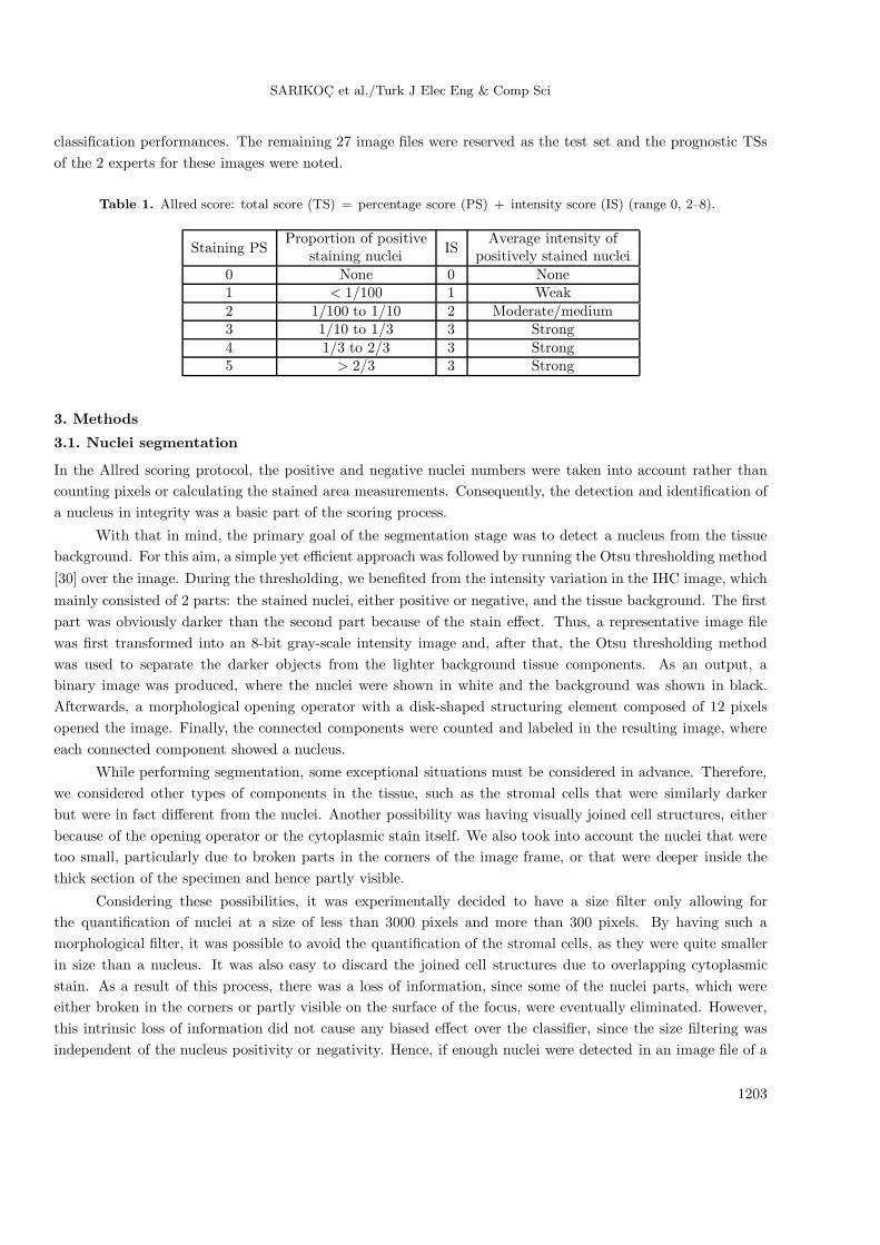
Table 1. Allred score: total score (TS) = percentage score (PS) + intensity score (IS) (range 0, 2–8).

Staining PSProportion of positive

ISAverage intensity of

staining nuclei positively stained nuclei0 None 0 None1 < 1/100 1 Weak2 1/100 to 1/10 2 Moderate/medium3 1/10 to 1/3 3 Strong4 1/3 to 2/3 3 Strong5 > 2/3 3 Strong

3. Methods

3.1. Nuclei segmentation

In the Allred scoring protocol, the positive and negative nuclei numbers were taken into account rather thancounting pixels or calculating the stained area measurements. Consequently, the detection and identification ofa nucleus in integrity was a basic part of the scoring process.

With that in mind, the primary goal of the segmentation stage was to detect a nucleus from the tissuebackground. For this aim, a simple yet efficient approach was followed by running the Otsu thresholding method[30] over the image. During the thresholding, we benefited from the intensity variation in the IHC image, whichmainly consisted of 2 parts: the stained nuclei, either positive or negative, and the tissue background. The firstpart was obviously darker than the second part because of the stain effect. Thus, a representative image filewas first transformed into an 8-bit gray-scale intensity image and, after that, the Otsu thresholding methodwas used to separate the darker objects from the lighter background tissue components. As an output, abinary image was produced, where the nuclei were shown in white and the background was shown in black.Afterwards, a morphological opening operator with a disk-shaped structuring element composed of 12 pixelsopened the image. Finally, the connected components were counted and labeled in the resulting image, whereeach connected component showed a nucleus.

While performing segmentation, some exceptional situations must be considered in advance. Therefore,we considered other types of components in the tissue, such as the stromal cells that were similarly darkerbut were in fact different from the nuclei. Another possibility was having visually joined cell structures, eitherbecause of the opening operator or the cytoplasmic stain itself. We also took into account the nuclei that weretoo small, particularly due to broken parts in the corners of the image frame, or that were deeper inside thethick section of the specimen and hence partly visible.

Considering these possibilities, it was experimentally decided to have a size filter only allowing forthe quantification of nuclei at a size of less than 3000 pixels and more than 300 pixels. By having such amorphological filter, it was possible to avoid the quantification of the stromal cells, as they were quite smallerin size than a nucleus. It was also easy to discard the joined cell structures due to overlapping cytoplasmicstain. As a result of this process, there was a loss of information, since some of the nuclei parts, which wereeither broken in the corners or partly visible on the surface of the focus, were eventually eliminated. However,this intrinsic loss of information did not cause any biased effect over the classifier, since the size filtering wasindependent of the nucleus positivity or negativity. Hence, if enough nuclei were detected in an image file of a

1203


representative region, the image file could be used as a reference input for all types of the feature set combinationexperiments.

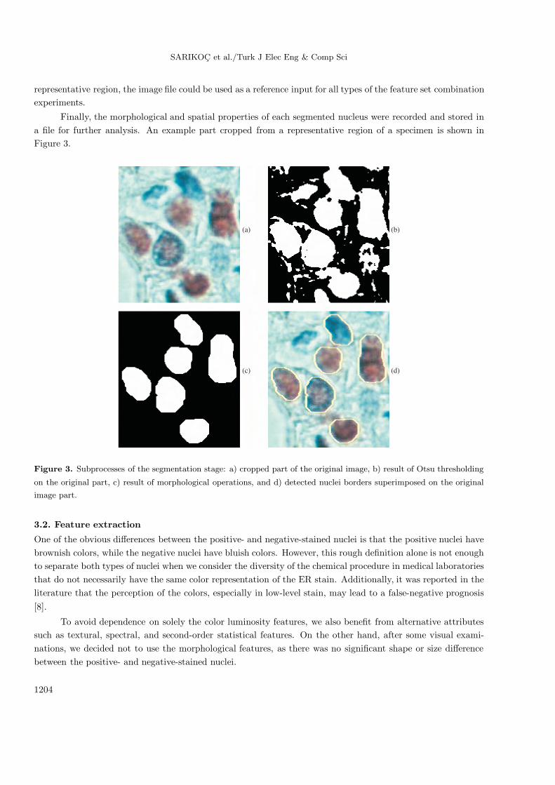
Finally, the morphological and spatial properties of each segmented nucleus were recorded and stored ina file for further analysis. An example part cropped from a representative region of a specimen is shown inFigure 3.

(a) (b)

(c) (d)

Figure 3. Subprocesses of the segmentation stage: a) cropped part of the original image, b) result of Otsu thresholding

on the original part, c) result of morphological operations, and d) detected nuclei borders superimposed on the original

image part.

3.2. Feature extraction

One of the obvious differences between the positive- and negative-stained nuclei is that the positive nuclei havebrownish colors, while the negative nuclei have bluish colors. However, this rough definition alone is not enoughto separate both types of nuclei when we consider the diversity of the chemical procedure in medical laboratoriesthat do not necessarily have the same color representation of the ER stain. Additionally, it was reported in theliterature that the perception of the colors, especially in low-level stain, may lead to a false-negative prognosis[8].

To avoid dependence on solely the color luminosity features, we also benefit from alternative attributessuch as textural, spectral, and second-order statistical features. On the other hand, after some visual exami-nations, we decided not to use the morphological features, as there was no significant shape or size differencebetween the positive- and negative-stained nuclei.

1204


In total, 144 features were extracted from each nucleus, where all of the features were generated from theimage area inside the border of the nucleus.

3.2.1. First-order statistical featuresThe statistics on an intensity histogram of an image can be used as descriptive attributes. In this work, wecalculated 6 different statistical properties of the intensity histogram, which were the mean/average, contrast,

smoothness, uniformity, third moment, and entropy [35]. Consequently, by extracting these features from eachRGB channel, and additionally from a gray-level transform, a total of 24 first-order statistical features werecomputed.

3.2.2. Second-order statistical features

Even though it is possible to get information about the intensity distribution of an image, the placementinformation for some specific intensity values is not known without examining the second-order statisticalfeatures. Therefore, structural descriptors like the cooccurrence matrix properties were calculated. To formthe intensity cooccurrence matrix from an 8-bit color channel, the intensity values were quantized at 8 differentlevels; hence, an 8 × 8-bit cooccurrence matrix was obtained. During this formation, the pixel of interestand its neighbor on the right-hand side were regarded. Thus, 8 structural features, autocorrelation, contrast,correlation, dissimilarity, energy, entropy, homogeneity, and the sum of squares, were calculated from eachcooccurrence matrix [36–38]. Finally, 32 second-order statistical features were generated from the color channelsof the RGB and from 1 gray-level transform of the nucleus image.

3.2.3. Laws’ texture energy features

The existence of some specific types of intensity variations in an image texture can be determined with smallconvolution kernels. Stemming from this idea, Laws’ texture energy images indicate the level, edge, spot, wave,and ripple appearance inside an image texture via the convolution kernels. The typical Laws’ kernels used fortexture discrimination are generated from 1-dimensional (1-D) kernels [39].

The convolution of a vertical 1-D kernel with a horizontal kernel or by repeating the same operation inreverse order yields a 2-D kernel. Hence, it is possible to generate 25 different 2-D kernels. If the directionalityof a pattern is not important when searching the existence of the pattern inside the image texture, then similar2-D kernels are combined so as to make the search complete with a lower number of 2-D kernels. By referringto “similar kernels”, we mean 2 types of kernels composed of the same 1-D kernels by convolving in a differentorder.

In our work, we have chosen to use 15 rationally invariant kernels, where 10 kernels came from the mutualconvolution rationally variant 1-D kernels and 5 self-convolved kernels were used as they are. Only the self-convolved 2-D kernel was discarded, since it did not have a zero-sum. Thus, 14 rationally invariant 2-D kernelswere generated, where 4 kernels were self-convolved and 10 kernels were the output of the mutual convolution.

By applying these kernels to each nucleus image and computing the energy function over them, a totalof 56 Laws’ texture energy images were obtained from the channels of the RGB nucleus image and 1 gray-leveltransform of the nucleus image.

3.2.4. Wavelet energy features

The periodicity of any pattern in the intensity variation could be useful to identify an object in an image. Forthis aim, spectral analysis was used with the idea that every signal could be considered as a linear summation of

1205


some basis functions, where all of the functions were orthogonal to each other and they were frequency-shiftedversions of one basic harmonic function.

Fourier transform stems from this approach; however, in this transform, it is not possible to detect thetime and localization information of any frequency component inside the signal, while it is possible to checkwhether or not any frequency component exists. To fill this gap, the wavelet transform is proposed, whichincludes one additional output dimension that is denoted for different scales of the basis function. By changingthe scale of the basis function, the frequency content of the signal, including the information of when or wherea specific harmonic occurs, can be obtained without losing the spatial representation of image signals.

By employing the wavelet transform [35] in 2 different scales, 8 different wavelet approximations of theoriginal nucleus image were produced. Later, the energy of each approximated image was calculated. Hence,in total, 32 different wavelet approximation-based energy features were generated from the RGB color channelsand gray-level transform of the nucleus image.

3.3. Feature elimination

We produced 144 features from each nucleus at the end of the feature generation stage. Considering the 384instances in the training set, such a high dimensionality of features as inputs may degrade the classificationsuccess or easily cause an overtraining error. Usually, it is suggested that the cardinality of the instancesmust be 10–30 times bigger than the cardinality of inputs of the classifier to avoid possible overtraining [40].Moreover, some features do not contribute extra information as they are highly correlated with each other.This redundancy in the inputs increases the computational complexity and time of the operation, where it mayalso cause a decrease in the classification or prediction accuracy [40]. For these reasons, it was experimentallydecided to employ a correlation-based heuristic feature selection algorithm in order to have a smaller inputdimensionality for the problem.

This heuristic approach relies on the hypothesis that “good feature subsets contain features highlycorrelated with the class, yet uncorrelated with each other”. Based on this idea [32], Eq. (2) describes theworth of a subset of features:

WorthS =k.rcf√

k + k.(k − 1).rff

, (2)

where WorthS is the heuristic worth of a feature subset S containing k features, rcf is the average feature–class

correlation, and rff is the average feature–feature intercorrelation. The prediction capability of the features inthe subset is represented by the numerator, while the existence of intercorrelations among the features of thesubset, or in other words the redundancy of the features, is indicated by the denominator. It was stated that“this formula actually is Pearson’s correlation, where all variables have been standardized” [32].

3.4. Classification

3.4.1. Performance measures of classification

Having selected some of the features as inputs for the classifier, it was expected from the model to be able toidentify the type and intensity range of a nucleus. There were 4 possibilities as the output, as shown in Table2. Here, the second possibility was not available in the dataset, and so a classifier was designed to give outputsaccording to the other 3 possibilities.

To measure the classification performance, we used 4 types of methods: correct classification performance,sensitivity and specificity analysis, confusion matrix, and receiver operating characteristic (ROC) curves. As its

1206


name implies, correct classification performance show us the percentage of instances that are correctly identifiedby the classifier. Given a predicted class of interest, the sensitivity and specificity values were calculatedaccording to the following expressions:

sensitivity =TP

TP + FN(%), (3)

specificity =TN

TN + FP(%), (4)

where TP , TN , FP , and FN are acronyms for true positive, true negative, false positive, and false negative,respectively.

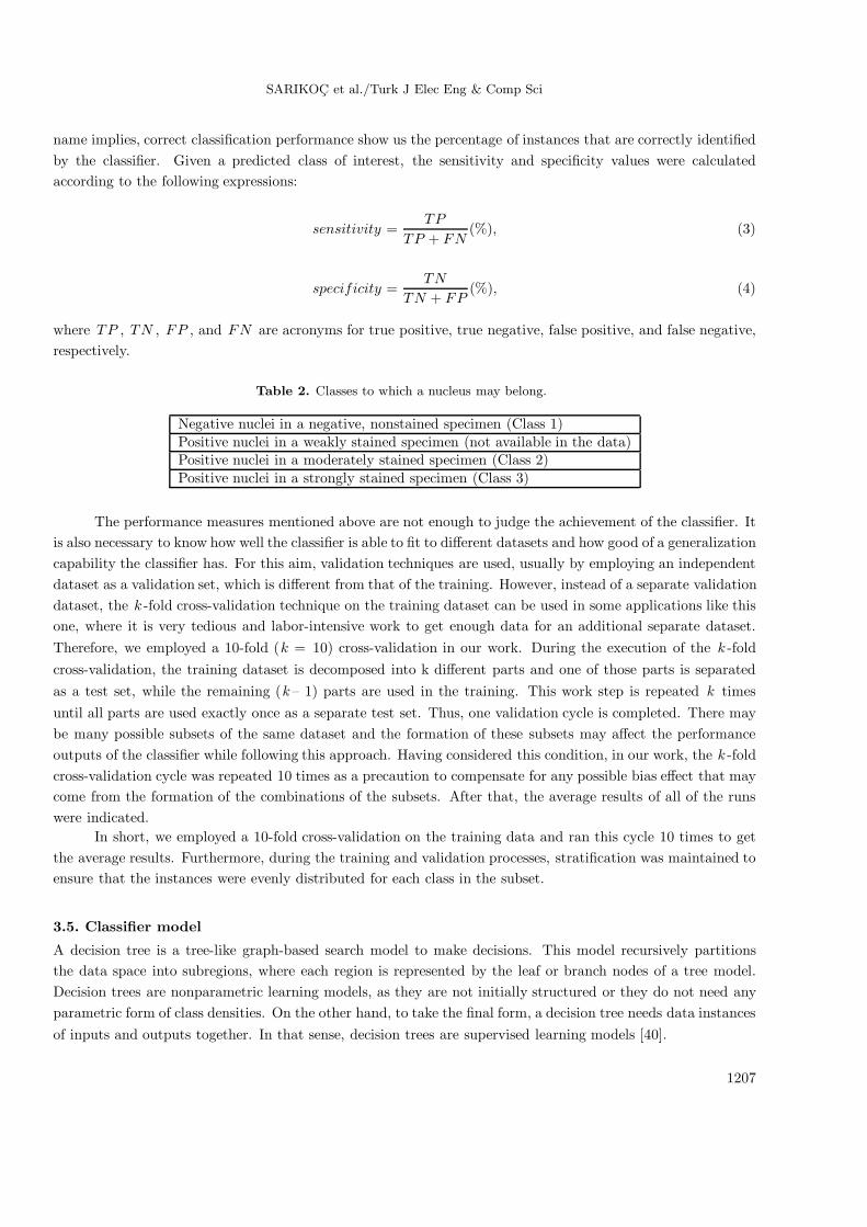
Table 2. Classes to which a nucleus may belong.

Negative nuclei in a negative, nonstained specimen (Class 1)Positive nuclei in a weakly stained specimen (not available in the data)Positive nuclei in a moderately stained specimen (Class 2)Positive nuclei in a strongly stained specimen (Class 3)

The performance measures mentioned above are not enough to judge the achievement of the classifier. Itis also necessary to know how well the classifier is able to fit to different datasets and how good of a generalizationcapability the classifier has. For this aim, validation techniques are used, usually by employing an independentdataset as a validation set, which is different from that of the training. However, instead of a separate validationdataset, the k -fold cross-validation technique on the training dataset can be used in some applications like thisone, where it is very tedious and labor-intensive work to get enough data for an additional separate dataset.Therefore, we employed a 10-fold (k = 10) cross-validation in our work. During the execution of the k -foldcross-validation, the training dataset is decomposed into k different parts and one of those parts is separatedas a test set, while the remaining (k– 1) parts are used in the training. This work step is repeated k timesuntil all parts are used exactly once as a separate test set. Thus, one validation cycle is completed. There maybe many possible subsets of the same dataset and the formation of these subsets may affect the performanceoutputs of the classifier while following this approach. Having considered this condition, in our work, the k -foldcross-validation cycle was repeated 10 times as a precaution to compensate for any possible bias effect that maycome from the formation of the combinations of the subsets. After that, the average results of all of the runswere indicated.

In short, we employed a 10-fold cross-validation on the training data and ran this cycle 10 times to getthe average results. Furthermore, during the training and validation processes, stratification was maintained toensure that the instances were evenly distributed for each class in the subset.

3.5. Classifier model

A decision tree is a tree-like graph-based search model to make decisions. This model recursively partitionsthe data space into subregions, where each region is represented by the leaf or branch nodes of a tree model.Decision trees are nonparametric learning models, as they are not initially structured or they do not need anyparametric form of class densities. On the other hand, to take the final form, a decision tree needs data instancesof inputs and outputs together. In that sense, decision trees are supervised learning models [40].

1207


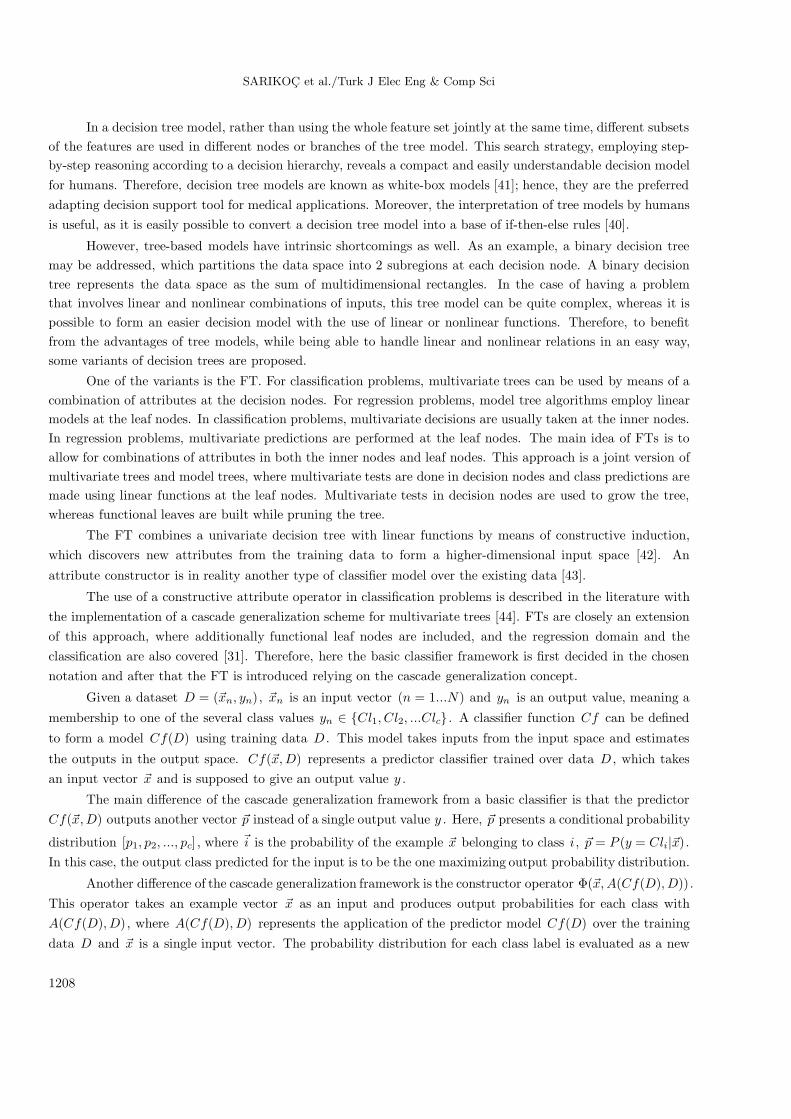
In a decision tree model, rather than using the whole feature set jointly at the same time, different subsetsof the features are used in different nodes or branches of the tree model. This search strategy, employing step-by-step reasoning according to a decision hierarchy, reveals a compact and easily understandable decision modelfor humans. Therefore, decision tree models are known as white-box models [41]; hence, they are the preferredadapting decision support tool for medical applications. Moreover, the interpretation of tree models by humansis useful, as it is easily possible to convert a decision tree model into a base of if-then-else rules [40].

However, tree-based models have intrinsic shortcomings as well. As an example, a binary decision treemay be addressed, which partitions the data space into 2 subregions at each decision node. A binary decisiontree represents the data space as the sum of multidimensional rectangles. In the case of having a problemthat involves linear and nonlinear combinations of inputs, this tree model can be quite complex, whereas it ispossible to form an easier decision model with the use of linear or nonlinear functions. Therefore, to benefitfrom the advantages of tree models, while being able to handle linear and nonlinear relations in an easy way,some variants of decision trees are proposed.

One of the variants is the FT. For classification problems, multivariate trees can be used by means of acombination of attributes at the decision nodes. For regression problems, model tree algorithms employ linearmodels at the leaf nodes. In classification problems, multivariate decisions are usually taken at the inner nodes.In regression problems, multivariate predictions are performed at the leaf nodes. The main idea of FTs is toallow for combinations of attributes in both the inner nodes and leaf nodes. This approach is a joint version ofmultivariate trees and model trees, where multivariate tests are done in decision nodes and class predictions aremade using linear functions at the leaf nodes. Multivariate tests in decision nodes are used to grow the tree,whereas functional leaves are built while pruning the tree.

The FT combines a univariate decision tree with linear functions by means of constructive induction,which discovers new attributes from the training data to form a higher-dimensional input space [42]. An

attribute constructor is in reality another type of classifier model over the existing data [43].

The use of a constructive attribute operator in classification problems is described in the literature withthe implementation of a cascade generalization scheme for multivariate trees [44]. FTs are closely an extensionof this approach, where additionally functional leaf nodes are included, and the regression domain and theclassification are also covered [31]. Therefore, here the basic classifier framework is first decided in the chosennotation and after that the FT is introduced relying on the cascade generalization concept.

Given a dataset D = (�xn, yn), �xn is an input vector (n = 1...N) and yn is an output value, meaning a

membership to one of the several class values yn ∈ {Cl1, Cl2, ...Clc} . A classifier function Cf can be defined

to form a model Cf(D) using training data D . This model takes inputs from the input space and estimates

the outputs in the output space. Cf(�x, D) represents a predictor classifier trained over data D , which takesan input vector �x and is supposed to give an output value y .

The main difference of the cascade generalization framework from a basic classifier is that the predictorCf(�x, D) outputs another vector �p instead of a single output value y . Here, �p presents a conditional probability

distribution [p1, p2, ..., pc] , where �i is the probability of the example �x belonging to class i , �p = P (y = Cli|�x).In this case, the output class predicted for the input is to be the one maximizing output probability distribution.

Another difference of the cascade generalization framework is the constructor operator Φ(�x, A(Cf(D), D)).This operator takes an example vector �x as an input and produces output probabilities for each class withA(Cf(D), D), where A(Cf(D), D) represents the application of the predictor model Cf(D) over the trainingdata D and �x is a single input vector. The probability distribution for each class label is evaluated as a new

1208


attribute; hence, new attributes are generated and added to existing actual ones, making the input set larger.When the Φ operator is applied to the whole instance of the dataset D , then a larger training set D′ is ob-tained. The number of the instances in D and D′ are the same, yet D′ has more attributes than D , wherethe cardinality existing classes and new attributes are the same.

Having more than one classifier, a sequential composition is performed, in which the Φ operator is appliedin each composition step using different classifiers. Given a training set L and a test T , and classifier 1 Cf1

and classifier 2 Cf2 , the sequential composition generates a training set L1new and a test set T 1

new by employingCf1 :

L1new = Φ(L, A(Cf1(L), L)), (5)

T 1new = Φ(T, A(Cf1(L), T )). (6)

Here, the prediction model Cf1(L) is applied to the training and test datasets, modifying them to generate newdatasets at composition level 1, which is indicated by the superscript of the dataset name. Another classifier,

Cf2 , learns from dataset L1new and is applied to the test dataset T 1

new , i.e. A(Cf2(L1new), T 1

new). When theoperation sequences of several classifiers are shown with dedicated operator symbol ∇ , then the sequence ofthe composition can be formally expressed as:

Cf2∇Cf1 = A(Cf2(L1new), T 1

new). (7)

In the case of having more than 2 classifiers, a composition of n classifiers is represented by:

Cfn∇Cfn−1∇Cfn−2...∇Cf1 = A(Cfn(Ln−1new), Tn−1

new ). (8)

The final model is given by the classifier Cfn after having done (n − 1) levels of compositions. Usingseveral classifiers and functions combined in such a scheme, it is expected to benefit from the knowledge ofthe representation of different approaches in the input space and the diverse searching capabilities of severalmethods together.

In addition to the FT model, we also examined the classification of the performance of some other models:the J48 decision tree of the Waikato Environment for Knowledge Analysis (WEKA), which is an implementation

of the C4.5 algorithm [45], and several support vector machine (SVM) models that are based on linear, quadratic,

and radial base functions [46].

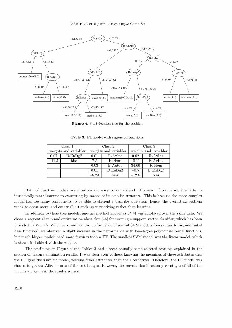
As stated before, a FT is able to use linear combinations of the attributes in the nodes and leaves, whilea univariate decision tree makes a simple probabilistic value test over a single attribute in a node. Thus, while aFT has the interpretation easiness of decision trees, it is also possible to exploit the generalization capability oflinear regression models without having complex tree structures. This benefit can be exemplified over a datasetof this prognosis application. When the J48 decision tree is constructed over the same dataset, such a decisiontree is formed as is given in Figure 4. The tree was built with a confidence factor of 0.25 and pruning wasenabled.

On the other hand, the FT method yields just a single node over the same dataset after the growing andpruning processes are completed. This single node contains regression functions, of which the bias and weightvalues for the features are given in Table 3. Having nominal class labels in the data is not an obstacle whenusing FTs, whereas it is necessary to double the number of classes by dichotomizing the existing nominal labelsso as to use linear regression models.

1209


B-AvInt

B-EnDg2

R-AvInt R-AvInt

R-EnAp1

B-AvInt

R-EnAp2 B-EnAp1

R-EnAp1 B-EnDg2

strong(120.0/2.0)

medium(3.0) none (3.0) medium (2.0)

medium(109.0/3.0)

medium(13.0)

strong(2.0)

none(17.0/1.0)

none(108.0)

strong(5.0) medium(2.0)

>137.94 ≤137.94

>124.98

≤124.98

>62,990.7

>176.7

≤62,990.7

≤376,153.38 >376,153.38

>14.78

≤14.78

>125,345.64 ≤125,345.64

>53,061.87

≤53,061.87

>13.12 ≤13.12

>140.08 ≤140.08

≤176.7

Figure 4. C4.5 decision tree for the problem.

Table 3. FT model with regression functions.

Class 1 Class 2 Class 3weights and variables weights and variables weights and variables0.07 B-EnDg2 0.01 R-AvInt 0.02 R-AvInt–11.3 bias 7.8 R-Hom –0.11 B-AvInt

0.03 B-Autoc 34.66 R-Hom0.01 B-EnDg2 –0.5 B-EnDg2–8.24 bias –12.6 bias

Both of the tree models are intuitive and easy to understand. However, if compared, the latter isintrinsically more immune to overfitting by means of its smaller structure. This is because the more complexmodel has too many components to be able to efficiently describe a relation; hence, the overfitting problemtends to occur more, and eventually it ends up memorizing rather than learning.

In addition to these tree models, another method known as SVM was employed over the same data. Wechose a sequential minimal optimization algorithm [46] for training a support vector classifier, which has been

provided by WEKA. When we examined the performance of several SVM models (linear, quadratic, and radial

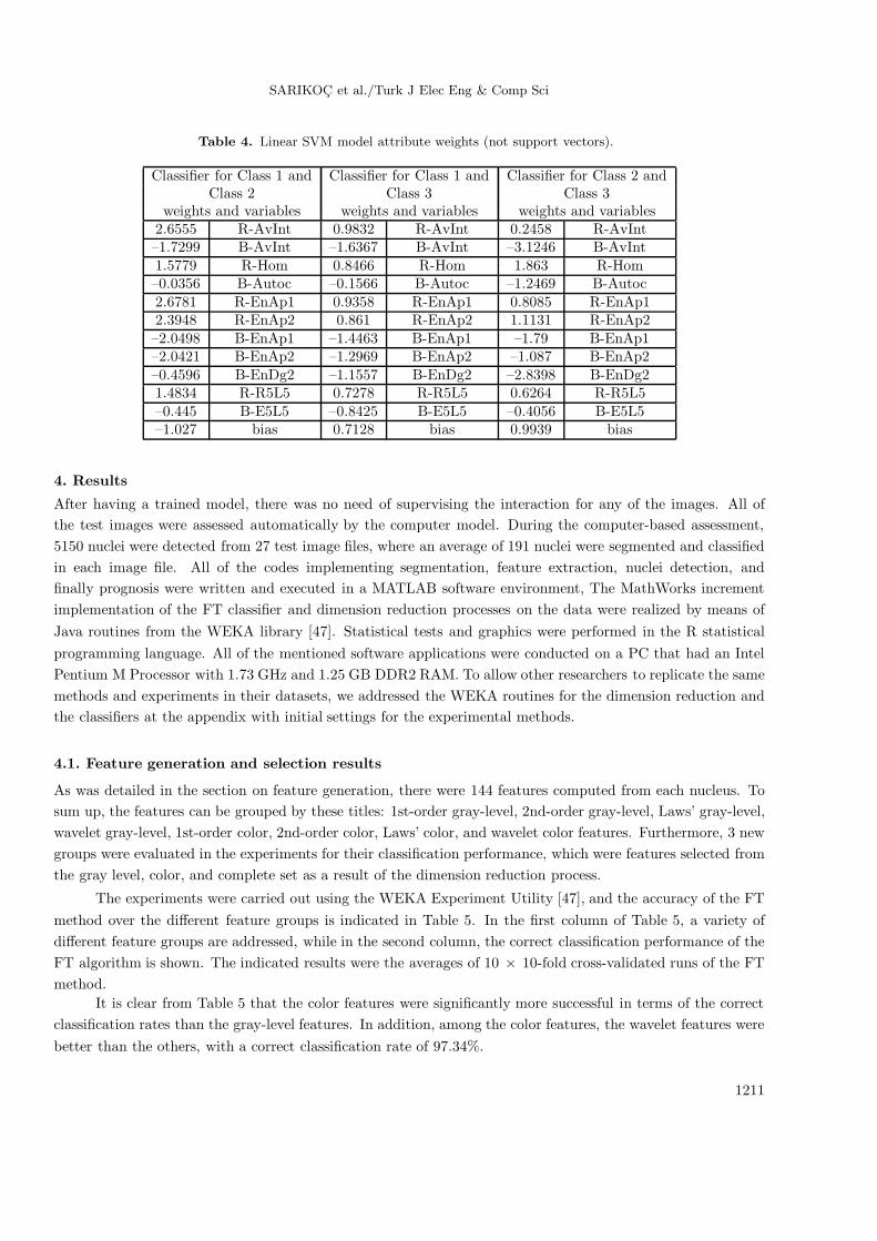
base function), we observed a slight increase in the performance with low-degree polynomial kernel functions,but much bigger models need more features than a FT. The smallest SVM model was the linear model, whichis shown in Table 4 with the weights.

The attributes in Figure 4 and Tables 3 and 4 were actually some selected features explained in thesection on feature elimination results. It was clear even without knowing the meanings of these attributes thatthe FT gave the simplest model, needing fewer attributes than the alternatives. Therefore, the FT model waschosen to get the Allred scores of the test images. However, the correct classification percentages of all of themodels are given in the results section.

1210


Table 4. Linear SVM model attribute weights (not support vectors).

Classifier for Class 1 and Classifier for Class 1 and Classifier for Class 2 andClass 2 Class 3 Class 3

weights and variables weights and variables weights and variables2.6555 R-AvInt 0.9832 R-AvInt 0.2458 R-AvInt–1.7299 B-AvInt –1.6367 B-AvInt –3.1246 B-AvInt1.5779 R-Hom 0.8466 R-Hom 1.863 R-Hom–0.0356 B-Autoc –0.1566 B-Autoc –1.2469 B-Autoc2.6781 R-EnAp1 0.9358 R-EnAp1 0.8085 R-EnAp12.3948 R-EnAp2 0.861 R-EnAp2 1.1131 R-EnAp2–2.0498 B-EnAp1 –1.4463 B-EnAp1 –1.79 B-EnAp1–2.0421 B-EnAp2 –1.2969 B-EnAp2 –1.087 B-EnAp2–0.4596 B-EnDg2 –1.1557 B-EnDg2 –2.8398 B-EnDg21.4834 R-R5L5 0.7278 R-R5L5 0.6264 R-R5L5–0.445 B-E5L5 –0.8425 B-E5L5 –0.4056 B-E5L5–1.027 bias 0.7128 bias 0.9939 bias

4. Results

After having a trained model, there was no need of supervising the interaction for any of the images. All ofthe test images were assessed automatically by the computer model. During the computer-based assessment,5150 nuclei were detected from 27 test image files, where an average of 191 nuclei were segmented and classifiedin each image file. All of the codes implementing segmentation, feature extraction, nuclei detection, andfinally prognosis were written and executed in a MATLAB software environment, The MathWorks incrementimplementation of the FT classifier and dimension reduction processes on the data were realized by means ofJava routines from the WEKA library [47]. Statistical tests and graphics were performed in the R statisticalprogramming language. All of the mentioned software applications were conducted on a PC that had an IntelPentium M Processor with 1.73 GHz and 1.25 GB DDR2 RAM. To allow other researchers to replicate the samemethods and experiments in their datasets, we addressed the WEKA routines for the dimension reduction andthe classifiers at the appendix with initial settings for the experimental methods.

4.1. Feature generation and selection results

As was detailed in the section on feature generation, there were 144 features computed from each nucleus. Tosum up, the features can be grouped by these titles: 1st-order gray-level, 2nd-order gray-level, Laws’ gray-level,wavelet gray-level, 1st-order color, 2nd-order color, Laws’ color, and wavelet color features. Furthermore, 3 newgroups were evaluated in the experiments for their classification performance, which were features selected fromthe gray level, color, and complete set as a result of the dimension reduction process.

The experiments were carried out using the WEKA Experiment Utility [47], and the accuracy of the FTmethod over the different feature groups is indicated in Table 5. In the first column of Table 5, a variety ofdifferent feature groups are addressed, while in the second column, the correct classification performance of theFT algorithm is shown. The indicated results were the averages of 10 × 10-fold cross-validated runs of the FTmethod.

It is clear from Table 5 that the color features were significantly more successful in terms of the correctclassification rates than the gray-level features. In addition, among the color features, the wavelet features werebetter than the others, with a correct classification rate of 97.34%.

1211


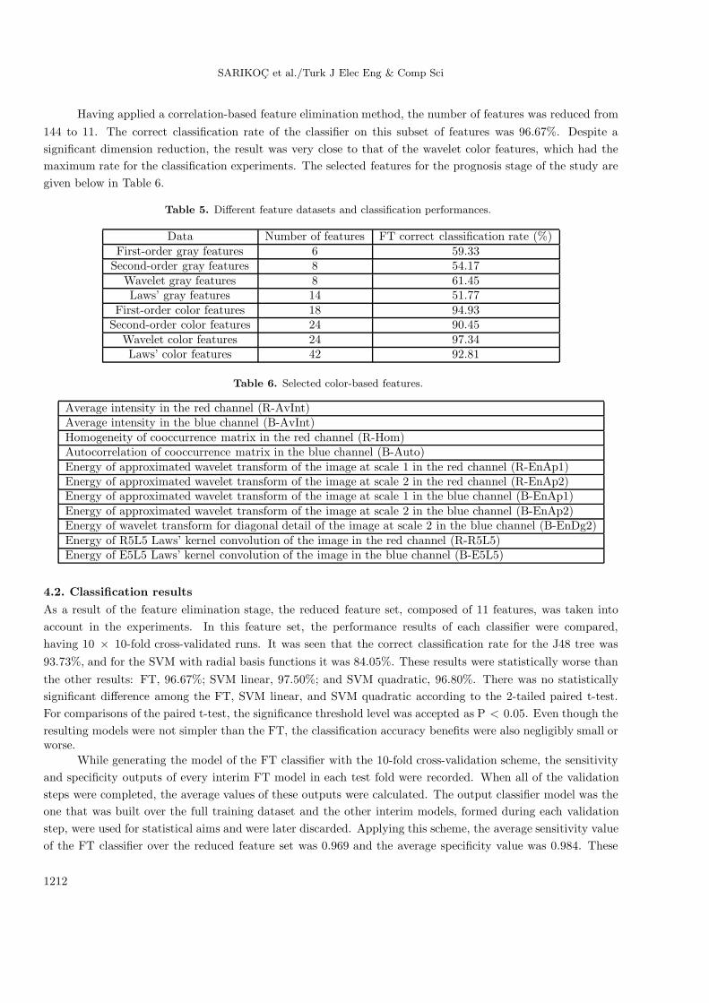
Having applied a correlation-based feature elimination method, the number of features was reduced from144 to 11. The correct classification rate of the classifier on this subset of features was 96.67%. Despite asignificant dimension reduction, the result was very close to that of the wavelet color features, which had themaximum rate for the classification experiments. The selected features for the prognosis stage of the study aregiven below in Table 6.

Table 5. Different feature datasets and classification performances.

Data Number of features FT correct classification rate (%)First-order gray features 6 59.33

Second-order gray features 8 54.17Wavelet gray features 8 61.45Laws’ gray features 14 51.77

First-order color features 18 94.93Second-order color features 24 90.45

Wavelet color features 24 97.34Laws’ color features 42 92.81

Table 6. Selected color-based features.

Average intensity in the red channel (R-AvInt)Average intensity in the blue channel (B-AvInt)Homogeneity of cooccurrence matrix in the red channel (R-Hom)Autocorrelation of cooccurrence matrix in the blue channel (B-Auto)Energy of approximated wavelet transform of the image at scale 1 in the red channel (R-EnAp1)Energy of approximated wavelet transform of the image at scale 2 in the red channel (R-EnAp2)Energy of approximated wavelet transform of the image at scale 1 in the blue channel (B-EnAp1)Energy of approximated wavelet transform of the image at scale 2 in the blue channel (B-EnAp2)Energy of wavelet transform for diagonal detail of the image at scale 2 in the blue channel (B-EnDg2)Energy of R5L5 Laws’ kernel convolution of the image in the red channel (R-R5L5)Energy of E5L5 Laws’ kernel convolution of the image in the blue channel (B-E5L5)

4.2. Classification resultsAs a result of the feature elimination stage, the reduced feature set, composed of 11 features, was taken intoaccount in the experiments. In this feature set, the performance results of each classifier were compared,having 10 × 10-fold cross-validated runs. It was seen that the correct classification rate for the J48 tree was93.73%, and for the SVM with radial basis functions it was 84.05%. These results were statistically worse thanthe other results: FT, 96.67%; SVM linear, 97.50%; and SVM quadratic, 96.80%. There was no statisticallysignificant difference among the FT, SVM linear, and SVM quadratic according to the 2-tailed paired t-test.For comparisons of the paired t-test, the significance threshold level was accepted as P < 0.05. Even though theresulting models were not simpler than the FT, the classification accuracy benefits were also negligibly small orworse.

While generating the model of the FT classifier with the 10-fold cross-validation scheme, the sensitivityand specificity outputs of every interim FT model in each test fold were recorded. When all of the validationsteps were completed, the average values of these outputs were calculated. The output classifier model was theone that was built over the full training dataset and the other interim models, formed during each validationstep, were used for statistical aims and were later discarded. Applying this scheme, the average sensitivity valueof the FT classifier over the reduced feature set was 0.969 and the average specificity value was 0.984. These

1212


values indicated for the classifier that it was highly probable that it would correctly recognize each nucleus andstaining type. Moreover, having examined the confusion matrix of the FT classifier in Table 7, it was seen thatthere were few misclassified instances out of the 384 training set nuclei.

Table 7. FT classifier confusion matrix.

Actual\predicted Class 1 Class 2 Class 3Class 1 (none) 127 1 0

Class 2 (moderate) 2 123 3Class 3 (strong) 0 6 122

The ROC curve is measured to show the performance of a classifier with regard to several threshold valuesdefining the decision. As the threshold value was changed, the separation capability of the classifier betweenthe target class and the remaining classes is depicted in Figure 5, where it can be observed that all of the classes(nonstained nuclei, moderately stained, and strongly stained positive nuclei) were robust against the changesof the threshold.

Finally, it was concluded from the classification performance measures that the FT method was able togive good separation results among the 3 classes.

0.9

1

0 0.2 0.4 0.6 0.8 1

nonstainedmoderatelystrongly

Tru

e po

sitiv

e ra

te

False positive rate

Figure 5. ROC curves of the classifiers for strongly, moderately, and nonstained nuclei.

4.3. Assessment results

We calculated the weighted kappa statistics over the assessment scores to measure the level of agreement betweenthe observers and the computer-based approach. As explained in the Section 2, ordinal scales were used as areference for scoring. Therefore, in this work, a quadratic scale of weights contributed to the calculation of thekappa statistics by considering different levels of agreements.

Kappa statistics can take values in the scale of [–1 1], where negative values mean disagreement, 0 indicatesagreement by chance, and the positive values imply agreement. In this range, –1 indicates perfect disagreementand 1 shows perfect agreement. Possible results according to kappa statistics and their interpretation are shownin Table 8 [48].

In addition to measuring the agreement, we also calculated a pair-wise correlation among the assessors bymeans of the Spearman’s rank order correlation coefficient. This is a well-known interrater agreement measure.

1213


Furthermore, the Wilcoxon pair-wise signed rank test was employed to see if there was a statistically significantdifference among the 3 assessors. Even though having a high correlation means a relation between the scores,it is also necessary to see whether or not the mean values of scores are close enough to each other, becauseit is possible to have good correlation between 2 series, each of which has very different mean values. In thissense, a significance test is supplemental to the agreement and correlation measures. For the significance test,we tested a null hypothesis, assuming that the average values of the assessments did not differ from each other.The decision threshold was defined as 0.05. If the P-value was bigger than 0.05, then the null hypotheses wasaccepted as correct; otherwise, it was not.

Table 8. Interpretation of Kappa values.

Value of K Strength of agreement< 0.20 Poor

0.21–0.40 Fair0.41–0.60 Moderate0.61–0.80 Good0.81–1.00 Very good

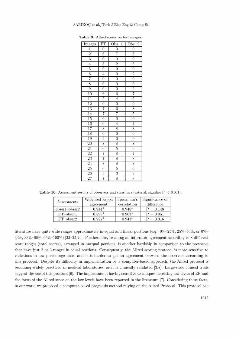
Referring to the Allred scoring protocol, the assessments of the computer-based approach and theobservers are given in Table 9. All of the measures for the assessments, i.e. the agreement, correlation, andsignificance test results, are demonstrated in Table 10.

When the kappa statistic results in Table 10 were compared with the reference values in Table 8, it wasobserved that there exists a very good agreement between the assessments of the pathologist observers and thecomputer-based method. In addition, it was noted that highly correlated scores were obtained among the 3assessors. Finally, considering the significance test outputs, it was concluded that there was no statisticallysignificant difference among the assessors.

5. Discussion and conclusionsIn our work, we found the kappa results (κ = 0.899 and κ = 0.927, P< 0.001), Spearman’s rank order

correlation coefficients (ρ = 0.963 and ρ = 0.943, P< 0.001) and Wilcoxon significance test results (P= 0.051

and P= 0.316) between the Allred scores of experts and the proposed automated model. Among the test

images, 25 of them (25/27) were correctly dichotomized as positive or negative compared to the average of theassessment scores of the 2 experts. Unfortunately, it is not directly possible to make a comparison betweenwhat we achieved and what was reported in the literature, because there are a variety of performance measuresreported for ER prognosis and a unified approach has not been adopted for this aim. Additionally, differentscoring procedures and decision cutoff values have been applied in the literature. Nonetheless, we will mentionsimilar works and their results so as to provide an overview of the dedicated area of literature. Hence, we thinkthat computer-based prognostic systems and the emerging need of objective benchmarking for the results ofdifferent laboratories will contribute to the standardization of performance measures. This also may enforcestandardization in the substages of clinical works from the fixation of tissues to the analysis of IHC results.

As seen in Table 1, the Allred scoring protocol is very sensitive to low-level staining variations because ofthe PS score ranges (0%–1%, 1%–10%, 10%–33%, 33%–66%, and 66%–100%). Given a positive nuclei detection

percentage of even less than 2%, there may be 3 different prognostic scores according to the Allred scoringprotocol. Considering the sensitiveness to such small intervals in terms of nucleus detection, having 1 or 2wrongly detected nuclei could easily alter the whole prognostic score, while some other protocols cited in the

1214


Table 9. Allred scores on test images.

Images FT Obs. 1 Obs. 21 0 0 02 6 7 63 0 0 04 5 2 55 0 0 06 4 0 27 0 0 08 0 0 09 0 0 210 6 6 711 5 4 512 0 0 013 7 6 814 7 7 515 0 0 016 6 4 417 8 8 818 0 0 019 4 0 020 8 8 821 6 5 622 7 8 723 7 8 824 8 8 825 6 5 626 5 3 327 7 8 8

Table 10. Assessment results of observers and classifiers (asterisk signifies P < 0.001).

AssessmentsWeighted kappa Spearman’s Significance of

agreement correlation differenceobser1–obser2 0.944* 0.948* P = 0.148

FT–obser1 0.899* 0.963* P = 0.051FT–obser2 0.927* 0.943* P = 0.316

literature have quite wide ranges approximately in equal and linear portions (e.g., 0%–25%, 25%–50%, or 0%–

33%, 33%–66%, 66%–100%) [23–25,29]. Furthermore, reaching an interrater agreement according to 8 different

score ranges (total scores), arranged in unequal portions, is another hardship in comparison to the protocolsthat have just 2 or 3 ranges in equal portions. Consequently, the Allred scoring protocol is more sensitive tovariations in low percentage cases and it is harder to get an agreement between the observers according tothis protocol. Despite its difficulty in implementation by a computer-based approach, the Allred protocol isbecoming widely practiced in medical laboratories, as it is clinically validated [3,8]. Large-scale clinical trials

suggest the use of this protocol [6]. The importance of having sensitive techniques detecting low levels of ER and

the focus of the Allred score on the low levels have been reported in the literature [7]. Considering these facts,in our work, we proposed a computer-based prognosis method relying on the Allred Protocol. This protocol has

1215


not been used in these previous studies, which also realized nuclei detection-based ER prognosis [23–25,27–29].

To the best of our knowledge, there are a few studies [25,26] detecting and counting nuclei while applyingAllred scoring for ER assessment. In a similar work, Krecsak et al. presented a computer-based automatedapproach for ER status evaluation [26] according to the Allred scoring protocol. Even though a higher agreement

score (κ = 0.981) was reported in that paper, unlike our study, the reported nilpotent quotient algorithm needsuser interaction and recalibration for the image to be assessed. Additionally, the color, intensity, and sizefeatures of the nuclei are considered in this recent work, whereas our study also computes additional featureslike wavelet transform energy features, giving higher correct classification rates according to Table 5 comparedto the first-order statistical features. In another work that conducted nucleus detection and quantification withthe same protocol, Sharangpani et al. [25] found a strong correlation between the algorithm-based values and

the subjective measurements (intraclass correlation: 0.77; 95% CI: 0.59–0.95) for the ER and the progesteronereceptor percentage nuclear positivity. In our work, the automated model achieved a higher level of correlationbetween the scores of the experts and the model.

Some of the studies used nuclei detection and counting approaches, as we did. These studies, givenbelow, referred to different scoring protocols. Kostopoulos et al. employed an unsupervised segmentationmethod, maintaining an adequate level of agreement (Kendall’s W = 0.79) between an automated computer-

based system and physician evaluations [25]. The same authors introduced a color texture-based image analysis

method resulting in an agreement level of Kendall’s W = 0.875, P < 0.001 [23]. In another work by the same

authors, a high correlation value (ρ = 0.89, P < 0.001) was reported using Spearman’s rank order correlationbetween the assessments of a histopathologist and an image analysis system that was based on texture energyfeatures [29]. Schnorrenberg et al. proposed a computer-aided detection system, the biopsy analysis support

system (BASS), that achieved Spearman’s rank order correlation levels of 0.78 < ρ < 0.86 (P < 0.001) forstrongly and very strongly stained nuclei. For the weakly stained nuclei, the correlation between the BASSsystem and the 2 experts was lower (ρ = 0.51 and ρ = 0.38, P < 0.001) [24].

Some previous studies in the literature relied on global threshold techniques, pixel- or area-based mea-sures, for assessment [10,12–22]. Among these studies, we focus on those giving agreement or correlation resultsbetween automated systems and the observers, as we have these types of results. We excluded the results ofCharpin et al., Furukawa et al., Hatanaka et al., and Lehr et al., as they compared automated systems withbiochemical procedures [10,17,13] or cytometric analysis [15]. In these works, the usage of some commercialsystems, i.e. SAMBA 200 by Charpin et al., WinROOF by Hatanaka et al., Adobe Photoshop by Lehr etal., and CAS 200 by Furukawa et al., were proposed. For the ER evaluation, the agreement rate between theautomated quantitative coronary analysis image analysis system and the manual scoring was reported as κ =0.84 by Diaz and Sneige [10]. Comparing the dichotomized scores between the automated Ariol machines and

the visual scores of 2 pathologists, the highest agreement rate was reported as κ = 0.9021 (95% CI: 0.8854–

0.9180) by Turbin et al. [12]. Gokhale et al. examined 2 commercially available systems: the ChromaVision

Automated Cellular Imaging System (ACIS) and the Applied Imaging Ariol SL-50. The highest correlationlevel according to the gamma statistics for the ER scores between the observers and the automated systemswas obtained by the ACIS as γ = 0.91 in [19]. Mofidi et al. observed a close correlation between the medianoptical density-based Adobe Photoshop mask implementation and the percentage positivity assessed manually

(r2 = 0.844, P< 0.0001) [14]. McClelland et al. reported a correlation level for all of the tumors as r = 0.919,P< 0.01, n = 94 between the percentage measurements of the positively stained nuclear area by the CAS 100system and the manually determined percentage of the stained cell nuclei, where a lower value of r = 0.821,

1216


P< 0.01, n = 68 was reported for the ER-positive cases only [16]. Chung et al. recorded a mean linear regres-sion of R= 0.8903 by comparing AQUA software results in a logarithmic scale with gold standard percentagescores in a study of 29 slides from 11 classic cases [18]. Camp et al. found a high degree of correlation (R=

0.884) between the AQUA-based automated system and the pathologist’s evaluation. They also compared thevariability of a pathologist’s evaluation and the automated analysis and reported that the automated analysishad a slightly better reproducibility (R = 0.824 versus R = 0.732) [20]. Lloyd et al. investigated 2 imagining

systems, Definiens (Munich, Germany) and Aperio Technologies (Vista, CA, USA), and concluded, without

giving statistical details, that both algorithms scored 10/10 cases within the range of the pathologist’s visual

labeling index [21]. Bolton et al. found that the agreement between the results of the pathologist and the

automated negative/positive and categorical scores were excellent for ER-α (κ range = 0.86–0.91), and lower

levels of agreement were seen for ER-β categorical scores (κ = 0.80–0.86). In this work, the performances of

3 different automated systems for IHC scoring were assessed: TMAx (Beecher Instruments, Sun Prairie, WI,

USA), Ariol (Applied Imaging, Grand Rapids, MI, USA), and TMALab II (Aperio) [22]. By utilizing the colordeconvolution algorithm, Tuominen et al. introduced the ImmunoRatio, which is a publicly available web-basedIHC analysis tool. It is reported that the calibrated ImmunoRatio has a strong linear relation (r = 0.98) withvisual assessments in terms of the percentage positive nuclei of a test set, including several types of biomarkers:estrogen, progesterone, and Ki-67 [27]. According to the results of Rexhepaj et al., an excellent correlation was

observed between the percentages of positive tumor nuclei by image analysis and manual analysis (Spearman’s

ρ = 0.9, P < 0.001). In the same paper, a strong correlation between image analysis and manual assess-

ment was indicated for the ER scores (Spearman’s ρ = 0.74, P< 0.001) [28]. Sharangpani et al. published asummary table for the properties of commercially available tools in addition to their custom-made algorithm[25]. A dedicated review of commercial devices can be found in [49]. Prasad et al. introduced a pixel color

quantification-based in-house application, TissueQuant, that provides the Spearman’s correlation (r = 0.53)

between the automated system and the visual scores for ER expression [50]. The common point of all of thesetools is that they are pixel- or area-based measures or global thresholding techniques for the luminosity features.

On the contrary, these studies based on global threshold techniques, pixel- or area-based percentagemeasures, nuclei detection, and counting-based approaches are used by experts in real medical practice. Inthat sense, our approach is more closely related to real medical applications by giving outputs directly fittingthe interpretations of the human experts. Moreover, by utilizing not only the luminosity thresholding butalso pattern recognition methods, the discrimination efficiency of the positive versus the negative nuclei wasincreased, as was seen in the results of the feature elimination stage, where 10 out of 11 selected features weretexture-based and only 1 remaining feature was an intensity feature.

In addition, using such a computer-based tool, it was easier to have a nuclei quantification analysis reportfor each specimen. Since there is diversity in medical laboratories regarding scoring systems and cutoff valuesfor status evaluation, there is an emerging trend to ask the laboratories to give their quantification values, suchas the number of detected nuclei or positivity percentage, rather than just expressing the qualitative assessmentresults as negative or positive. For this reason, we think that this computer-based approach can make it easierfor experts to record and report the documentation of quantitative data, justifying their decision, which is alsoa benefit providing the reproducibility of a prognosis.

Custom-made software and algorithms add value to the research of standardized automated IHC analysis.However, the application of these approaches by other researchers may involve time and extra effort. Consideringthis fact, we adopted a compact approach by utilizing one of the existing machine learning libraries [47]. We

1217


also addressed open-source Java codes to allow other researchers to replicate the method that we proposed here.In such an integrated and shared application environment allowing for ready-to-use libraries, it would be easierto explore the achievement of alternative machine learning methods. Hence, we expect that the research in thisarea might increase by facilitating the usage of different machine learning methods in available tools. Moreover,the need for benchmarking of the results from several machine learning algorithms on the same basis may leadto standard assessment performance measures.

Another contribution of this paper was the use of the FT method as a classifier for this medical application.Even though there might be many different alternative classifiers for this study, it was taken into account thattree-based approaches give compactly stored robust models. Unlike other classifiers described as a black boxbecause of their complicated structure, tree models are easy to understand for experts and could also provideinsight into the existing data structure [40,41]. On the other hand, it is known that decision trees have somedrawbacks, such as the difficulty in designing an optimal tree with fewer nodes and the need to define the searchspace with parallel orthogonal rectangles in the case of using binary trees. To circumvent these weaknesses [31],the FT method was intentionally chosen from among the other tree-based methods.

Having implemented the FT classifier, it was observed in the assessment results that there was a very goodagreement between the scores of the observers and the computer-based approach. In addition, the assessmentsof all of the raters were highly correlated and they did not have a statistically significant difference. However,it was also noteworthy that the agreement between the FT classifier and observer 1 was slightly lower andthe significance of difference was nearly at the border of the threshold. Still, all of these findings showed thepractical potential of the work. It could be possible to increase the accuracy further, with a wider range of dataand optimized substages such as an investigation performance of several of the dimension reduction techniquesor several types of classifiers over the problem. Furthermore, although the preprocessing of the images wasnot carried out in this work, the effects of the preprocessing, performance comparison of different segmentationprocedures, and morphological operators can be investigated as a future study.

As to the limitations of this application, 4 main points must be addressed. First, the region of intereston a slide must be chosen by an expert in advance. Second, the same fixation procedures must be appliedfor all of the tissue samples. Third, the images that have a cytoplasmic stain, artifacts, or blurred patternsmust be discarded, because some parts of the stained cytoplasm are detected as positive nuclei by the model.Hence, it erroneously tends to give positive scores when an image with cytoplasmic stain is involved. As the lastlimitation, some additional time for the algorithmic process must be given at least once, as supervised classifieralgorithms need a training process before their implementation.

All in all, after obtaining the experimental results, it was seen that image analysis with FT classifierscould be useful to pathologists as a support tool. This may reduce intralaboratory variation and contributeto the increase of the interobserver and intraobserver reproducibility for ER status evaluation according to theAllred scoring protocol.

6. Appendix

WEKA routines used in this work for the classifiers and feature elimination technique were given with the initialsettings in Table 11, and these codes can be freely experimented with [47].

1218


Table 11. Classifiers and Java routines of WEKA with initial settings.

Classifier or algorithms WEKA routines and initial settingsDimension reduction weka.attributeSelection.CfsSubsetEval

Functional trees trees.FT ’-I 15 -F 0 -M 15 –W 0.0’C4.5 decision tree trees.J48 ’-C 0.25 -M 2’

SVM linear functions.SMO ’-C 1.0 -L 0.0010 -P 1.0E-12 -N 0 -V -1 -W 1-K\“functions.supportVector.PolyKernel -C 250007 -E 1.0\”’

SVM quadratic functions.SMO ’-C 1.0 -L 0.0010 -P 1.0E-12 -N 0 -V -1 -W 1-K\“functions.supportVector.PolyKernel -C 250007 -E 2.0\”’

SVM radial base function functions.SMO ’-C 1.0 -L 0.0010 -P 1.0E-12 -N 0 -V -1 -W 1-K\“functions.supportVector.RBFKernel -C 250007 -G 0.01\”’

Acknowledgments

This work was supported by the Research Fund of Erciyes University, Project No. FBD-08-355. Many thanksto Pathologist Dr Fatma Aykas for capturing the images from the slides and to Dr Mehtap Kala for markingthe nuclei on the images.

References

[1] G. Daglar, Y.N. Yuksek, A.U. Gozalan, T. Tutuncu, Y. Gungor, N.A. Kama, “The prognostic value of histological

grade in the outcome of patients with invasive breast cancer”, Turkish Journal of Medical Sciences, Vol. 40, pp.

7–15, 2010.

[2] S. Sommer, S.A. Fuqua, “Estrogen receptor and breast cancer”, Seminars in Cancer Biology, Vol. 11, pp. 339–352,

2001.

[3] J.M. Harvey, G.M. Clark, C.K. Osborne, D.C. Allred, “Estrogen receptor status by immunohistochemistry is

superior to the ligand-binding assay for predicting response to adjuvant endocrine therapy in breast cancer”, Journal

of Clinical Oncology, Vol. 17, pp. 1474–1481, 1999.

[4] L.J. Layfield, D. Gupta, E.E. Mooney, “Assessment of tissue estrogen and progesterone receptor levels: a survey of

current practice, techniques, and quantitation methods”, Breast Journal, Vol. 6, pp. 189–196, 2000.

[5] R.A. Walker, “Quantification of immunohistochemistry – issues concerning methods, utility and semiquantitative

assessment I”, Histopathology, Vol. 49, pp. 406–410, 2006.

[6] S. Umemura, J. Itoh, H. Itoh, A. Serizawa, Y. Saito, Y. Suzuki, Y. Tokuda, T. Tajima, R.Y. Osamura, “Immuno-

histochemical evaluation of hormone receptors in breast cancer: which scoring system is suitable for highly sensitive

procedures?” Applied Immunohistochemistry & Molecular Morphology, Vol. 12, pp. 8–13, 2004.

[7] R.A. Walker, “Immunohistochemical markers as predictive tools for breast cancer”, Journal of Clinical Pathology,

Vol. 61, pp. 689–696, 2008.

[8] A. Qureshi, S. Pervez, “Allred scoring for ER reporting and its impact in clearly distinguishing ER negative from

ER positive breast cancers”, Journal of the Pakistan Medical Association, Vol. 60, pp. 350–353, 2010.

[9] T. Rudiger, H. Hofler, H.H. Kreipe, H. Nizze, U. Pfeifer, H. Stein, F.E. Dallenbach, H.P. Fischer, M. Mengel, R.

Wasielewski, H.K. Muller-Hermelink, “Quality assurance in immunohistochemistry: results of an interlaboratory

trial involving 172 pathologists”, American Journal of Surgical Pathology, Vol. 26, pp. 873–882, 2002.

[10] L.K. Diaz, N. Sneige, “Estrogen receptor analysis for breast cancer: current issues and keys to increasing testing

accuracy”, Advances in Anatomic Pathology, Vol. 12, pp. 10–19, 2005.

[11] C. Charpin, L. Andrac, M.C. Habib, H. Vacheret, L. Xerri, B. Devictor, M.N. Lavaut, M. Toga, “Immunodetection

in fine-needle aspirates and multiparametric (SAMBA) image analysis. Receptors (monoclonal antiestrogen and

antiprogesterone) and growth fraction (monoclonal Ki67) evaluation in breast carcinomas”, Cancer, Vol. 63, pp.

863–872, 1989.

1219


[12] D.A. Turbin, S. Leung, M.C.U. Cheang, H.A. Kennecke, K.D. Montgomery, S. McKinney, D.O. Treaba, N. Boyd,

L.C. Goldstein, S. Badve, A.M. Gown, M. Rijn, T.O. Nielsen, C.B. Gilks, D.G. Huntsman, “Automated quantitative

analysis of estrogen receptor expression in breast carcinoma does not differ from expert pathologist scoring: a tissue

microarray study of 3,484 cases”, Breast Cancer Research and Treatment, Vol. 110, pp. 417–426, 2008.

[13] H.A. Lehr, D.A. Mankoff, D. Corwin, G. Santeusanio, A.M. Gown, “Application of Photoshop-based image analysis

to quantification of hormone receptor expression in breast cancer”, Journal of Histochemistry & Cytochemistry,

Vol. 45, pp. 1559–1566, 1997.

[14] R. Mofidi, R. Walsh, P.F. Ridgway, T. Crotty, E.W. McDermott, T.V. Keaveny, M.J. Duffy, A.D. Hill, N. O’Higgins,

“Objective measurement of breast cancer oestrogen receptor status through digital image analysis”, European

Journal of Surgical Oncology, Vol. 29, pp. 20–24, 2003.

[15] Y. Hatanaka, K. Hashizume, K. Nitta, T. Kato, I. Itoh, Y. Tani, “Cytometrical image analysis for immunohis-

tochemical hormone receptor status in breast carcinomas”, Pathology International, Vol. 53, pp. 693–699, 2003.

[16] R.A. McClelland, P. Finlay, K.J. Walker, D. Nicholson, J.F.R. Robertson, R.W. Blamey, R.I. Nicholson, “Automated

quantitation of immunocytochemically localized estrogen receptors in human breast cancer”, Cancer Research, Vol.

50, pp. 3545–3550, 1990.

[17] Y. Furukawa, I. Kimijima, R. Abe, “Immunohistochemical image analysis of estrogen and progesterone receptors

in breast cancer”, Breast Cancer, Vol. 5, pp. 375–380, 1998.

[18] G.G. Chung, M.P. Zerkowski, S. Ghosh, R.L. Camp, D.L. Rimm, “Quantitative analysis of estrogen receptor

heterogeneity in breast cancer”, Laboratory Investigation, Vol. 87, pp. 662–669, 2007.

[19] S. Gokhale, D. Rosen, N. Sneige, L.K. Diaz, E. Resetkova, A. Sahin, J. Liu, C.T. Albarracin, “Assessment of two

automated imaging systems in evaluating estrogen receptor status in breast carcinoma”, Applied Immunohisto-

chemistry & Molecular Morphology, Vol. 15, pp. 451–455, 2007.

[20] R.L. Camp, G.G. Chung, D.L. Rimm, “Automated subcellular localization and quantification of protein expression

in tissue microarrays”, Nature Medicine, Vol. 8, pp. 1323–1328, 2002.

[21] M.C. Lloyd, P.A. Nandyala, C.N. Purohit, N. Burke, D. Coppola, M.M. Bui, “Using image analysis as a tool for

assessment of prognostic and predictive biomarkers for breast cancer: how reliable is it?”, Journal of Pathology

Informatics, Vol. 1, p. 29, 2010.

[22] K.L. Bolton, M.G. Closas, R.M. Pfeiffer, M.A. Duggan, W.J. Howat, S.M. Hewitt, X.R. Yang, R. Cornelison, S.L.

Anzick, P. Meltzer, S. Davis, P. Lenz, J.D. Figueroa, P.D.P. Pharoah, M.E. Sherman, “Assessment of automated

image analysis of breast cancer tissue microarrays for epidemiologic studies”, Cancer Epidemiology, Biomarkers &

Prevention, Vol. 19, pp. 992–999, 2010.

[23] S. Kostopoulos, D. Cavouras, A. Daskalakis, P. Bougioukos, P. Georgiadis, G.C. Kagadis, I. Kalatzis, P. Ravazoula,

G. Nikiforidis, “Colour-texture based image analysis method for assessing the hormone receptors status in breast

tissue sections”, Conference Proceedings of the IEEE Engineering in Medicine and Biology Society, pp. 4985–4988,

2007.

[24] F. Schnorrenberg, N. Tsapatsoulis, C.S. Pattichis, C.N. Schizas, S. Kollias, M. Vassiliou, A. Adamou, K. Kyriacou,

“Improved detection of breast cancer nuclei using modular neural networks”, IEEE Engineering in Medicine and

Biology Magazine, Vol. 19, pp. 48–63, 2000.

[25] S. Kostopoulos, D. Cavouras, A. Daskalakis, P. Ravazoula, G. Nikiforidis, “Image analysis system for assessing

the estrogen receptor’s positive status in breast tissue carcinomas”, Proceedings of the International Special Topic

Conference on Information Technology in Biomedicine, 2006.

[26] L. Krecsak, T. Micsik, G. Kiszler, T. Krenacs, D. Szabo, V. Jonas, G. Csaszar, L. Czuni, P. Gurzo, L. Ficsor, B.

Molnar, “Technical note on the validation of a semi-automated image analysis software application for estrogen and

progesterone receptor detection in breast cancer”, Diagnostic Pathology, Vol. 6, p. 6, 2011.

[27] V.J Tuominen, S. Ruotoistenmaki, A. Viitanen, M. Jumppanen, J. Isola, “ImmunoRatio: a publicly available web

application for quantitative image analysis of estrogen receptor (ER), progesterone receptor (PR), and Ki-67”,

Breast Cancer Research, Vol. 12, R56, 2010.

1220


[28] E. Rexhepaj, D.J. Brennan, P. Holloway, E.W. Kay, A.H. McCann, G. Landberg, M.J. Duffy, K. Jirstrom, W.M.

Gallagher, “Novel image analysis approach for quantifying expression of nuclear proteins assessed by immunohis-

tochemistry: application to measurement of oestrogen and progesterone receptor levels in breast cancer”, Breast

Cancer Research, Vol. 10, R89, 2008.

[29] S. Kostopoulos, D. Cavouras, A. Daskalakis, I. Kalatzis, P. Bougioukos, G. Kagadis, P. Ravazoula, G. Nikiforidis,

“Assessing estrogen receptors’ status by texture analysis of breast tissue specimens and pattern recognition meth-

ods”, Proceedings of the 12th International Conference on Computer Analysis of Images and Patterns, pp. 221–228,

2007.

[30] N. Otsu, “A threshold selection method from gray-level histograms”, IEEE Transactions on Systems, Man, and

Cybernetics, Vol. 9, pp. 62–66, 1979.

[31] J. Gama, “Functional trees”, Machine Learning, Vol. 55, pp. 219–250, 2004.

[32] M.A. Hall, “Correlation-based feature subset selection for machine learning”, PhD, Department of Computer

Science, University of Waikato, 1999.

[33] I.O. Ellis, S.J. Schnitt, X. Sastre-Garau, G. Bussolati, F.A. Tavassoli, V. Eusebi, J.L. Peterse, K. Mukai, L. Tabar,

J. Jacquemier, C.J. Cornelisse, A.J. Sasco, R. Kaaks, P. Pisani, D.E. Goldgar, P. Devilee, M.J. Cleton-Jansen, A.L.

Borresen-Dale, L. van ’t Veer, A. Sapino, Invasive breast carcinoma, in: I.O. Ellis, S.J. Schnitt, X. Sastre-Garau,

eds., World Health Organization Classification of Tumors. Pathology and Genetics of Tumours of the Breast and

Female Genital Organs, Lyon, France, IARC Press, pp. 40–42, 2003.

[34] C.W. Elston, I.O. Ellis, “Pathological prognostic factors in breast cancer I. The value of histological grade in breast

cancer: experience from a large study with long-term follow-up”, Histopathology, Vol. 19, pp. 403–410, 1991.

[35] R.C. Gonzalez, R.E. Woods, Digital Image Processing, New Jersey, Prentice Hall, 2002.

[36] R.M. Haralick, K. Shanmugam, I.H. Dinstein, “Textural features for image classification”, IEEE Transactions on

Systems, Man, and Cybernetics, Vol. 3, pp. 610–621, 1973.

[37] D.A. Clausi, “An analysis of co-occurrence texture statistics as a function of grey level quantization”, Canadian

Journal of Remote Sensing, Vol. 28, pp. 45–62, 2002.

[38] L. Soh, C. Tsatsoulis, “Texture analysis of SAR sea ice imagery using gray level co-occurrence matrices”, IEEE

Transactions on Geoscience and Remote Sensing, Vol. 37, pp. 780–795, 1999.

[39] M. Sonka, V. Hlavac, R. Boyle, Image Processing, Analysis and Machine Vision, International Student Edition,

Nashville, Thomas Nelson, 2008.

[40] E. Alpaydin, Introduction to Machine Learning, Cambridge, MIT Press, 2004.

[41] A.R. Webb, Statistical Pattern Recognition, 2nd ed., New York, Wiley, 2002.

[42] C.J. Matheus, L. Rendell, “Constructive induction on decision trees”, Proceedings of the 11th International Joint

Conference on Artificial Intelligence, Vol. 1, pp. 645–650, 1989.

[43] J. Gama, “Probabilistic linear tree”, International Conference on Machine Learning, pp. 134–142, 1997.

[44] J. Gama, P. Brazdil, “Cascade generalization”, Machine Learning, Vol. 41, pp. 315–343, 2000.

[45] R. Quinlan, C4.5: Programs for Machine Learning, San Mateo, CA, USA, Morgan Kaufmann Publishers, 1993.

[46] J. Platt, “Fast training of support vector machines using sequential minimal optimization”, in: B. Schoelkopf, C.

Burges, A. Smola, eds., Advances in Kernel Methods – Support Vector Learning, Cambridge, MIT Press, 1999.

[47] M. Hall, E. Frank, G. Holmes, B. Pfahringer, P. Reutemann, I.H. Witten, “The WEKA data mining software: an

update”, ACM SIGKDD Explorations Newsletter, Vol. 11, 2009.

[48] D.G. Altman, Practical Statistics for Medical Research, London, Chapman and Hall, 1991.

[49] M. Cregger, A.J. Berger, D.L. Rimm, “Immunohistochemistry and quantitative analysis of protein expression”,

Archives of Pathology and Laboratory Medicine, Vol. 130, pp. 1026–1030, 2006.

[50] K. Prasad, P.B. Kumar, M. Chakravarthy, G. Prabhu, “Applications of ‘TissueQuant’- a color intensity quantifica-

tion tool for medical research”, Computer Methods and Programs in Biomedicine, Vol. 106, pp. 27–36, 2011.

1221

An automated prognosis system for estrogen hormone status assessment in breast cancer tissue samples

Documents

Transcript of An automated prognosis system for estrogen hormone status assessment in breast cancer tissue samples