ORIGINAL PAPER

An approach to parameters estimation of a chromatographymodel using a clustering genetic algorithm based inverse model

Mirtha Irizar Mesa • Orestes Llanes-Santiago • Francisco Herrera Fernandez •

David Curbelo Rodrıguez • Antonio Jose Da Silva Neto •

Leoncio Diogenes T. Camara

Published online: 4 August 2010

� Springer-Verlag 2010

Abstract Genetic algorithms are tools for searching in

complex spaces and they have been used successfully in

the system identification solution that is an inverse prob-

lem. Chromatography models are represented by systems

of partial differential equations with non-linear parameters

which are, in general, difficult to estimate many times. In

this work a genetic algorithm is used to solve the inverse

problem of parameters estimation in a model of protein

adsorption by batch chromatography process. Each popu-

lation individual represents a supposed condition to the

direct solution of the partial differential equation system,

so the computation of the fitness can be time consuming if

the population is large. To avoid this difficulty, the

implemented genetic algorithm divides the population into

clusters, whose representatives are evaluated, while the

fitness of the remaining individuals is calculated in func-

tion of their distances from the representatives. Simulation

and practical studies illustrate the computational time

saving of the proposed genetic algorithm and show that it is

an effective solution method for this type of application.

Keywords Genetic algorithms � Inverse problem �Parameter estimation � Adsorption chromatography

1 Introduction

System identification is a fundamental tool in the analysis

of systems. It consists in the construction of mathematical

models of dynamic systems starting from experimental

data of measurement. Such models have important appli-

cations in many areas as diagnosis, simulation, prediction

and control. In general, the identification process has three

successive phases: preparation, estimation and validation.

It is typically an iterative procedure, where the user criteria

are mixed with formal calculations, an extensive manipu-

lation of the data and computer algorithms. There are many

contributions on this topic in the last five decades and some

representative examples are: Eykhoff (1974), Ljung (1999),

Ljung and Glad (1994).

There are a large number of identification methods and

they can be classified according to different approaches

(Ljung 1999; Soderstrom and Stoica 1994). In one group

there are the parametric methods. In general, they require

the election of a possible structure model and a parameter

adjustment approach and estimation of parameters that

better adjust the model to experimental data. Model iden-

tification is defined as the experimental determination of

parameters that governs the dynamics and/or the non-linear

behavior, if the structure of process model is known (Ljung

M. Irizar Mesa (&) � O. Llanes-Santiago

Department of Automation and Computers, Technical University

of Havana (ISPJAE), Ciudad de La Habana, Cuba

e-mail: mirtha@electrica.cujae.edu.cu

O. Llanes-Santiago

e-mail: orestes@electrica.cujae.edu.cu

F. Herrera Fernandez

Department of Automation and Computational Systems,

Central University of Las Villas (UCLV), Villa Clara, Cuba

e-mail: herrera@fie.uclv.edu.cu

D. Curbelo Rodrıguez

Center of Molecular Immunology, Ciudad de la Habana, Cuba

e-mail: david@cim.sld.cu

A. J. Da Silva Neto � L. D. T. Camara

Departamento de Engenharia Mecanica e Energia, DEMEC,

IPRJ-UERJ, Nova Friburgo, Brazil

e-mail: ajsneto@iprj.uerj.br

L. D. T. Camara

e-mail: dcamara@iprj.uerj.br

123

Soft Comput (2011) 15:963–973

DOI 10.1007/s00500-010-0638-3

1999). Estimation of unknown parameters in a mathemat-

ical model starting from known data of the solution con-

stitutes an inverse problem (see Fig. 1). Taking into

account the results of an objective function which lets the

comparison between the experimental values and those

obtained from the model evaluation, the parameters are

upgraded successively by means of an inverse method until

a stopping condition. Such problems (Tarantola 2005) are

frequent and of great importance in chemical, physical and

pharmaceutical applications among many others.

Solution of inverse problems can vary drastically from

one problem to another. However, their general charac-

teristic is the same: a system output answer is measured

and the conditions to obtain it should be calculated.

Although there are adequate methods to solve general

inverse problems, in several cases those are not completely

effective or require an excessive computational time to

solve the wide spectrum of inverse problems that are

important to scientists and engineers. The most effective

methods for inverse problems solution include non-linear

optimization procedures, which can be applied virtually in

any case.

Classical algorithms for parameter estimation as an

optimization problem perform local searches around an

initial guess or require gradient information that may not

always be easily available. The gradient-based optimiza-

tion methods such as steepest descent, conjugate gradient,

Davidon–Fletcher–Powell, Broydon–Fletcher–Goldfarb–

Shanno (Fletcher 1987) and Levenberg–Marquardt (Dennis

and Schnabel 1983) can identify a local optimum around

the initial guess. The gradient-less techniques, such as

the downhill simplex method due to Nelder and Mead

(1965), require additional function evaluations and a search

direction is obtained at each major iteration. All of these

methods provide a local optimum, but frequently there are

multiple local solutions for this type of problem and the

convergence to the global solution cannot be guaranteed.

Evolutionary algorithms, a subfield of computational

intelligence, are search methods based on the mechanisms

of the genetics (Davis 1991; Goldberg 1989). Genetic

algorithm (GA) is a type of evolutionary algorithm that

constitutes a special and efficient method of stochastic

optimization and it has been used for the solution of dif-

ficult problems, where the objective functions do not have

good mathematical properties (Back 1997; Michalewicz

1992). These algorithms carry out their searches using a

population of possible solutions for the problem. They

implement the survival strategy of the best adapted, as a

form to find better solutions, that distinguishes them from

the traditional search methods. GAs have been useful in the

solution of many different problems which require the

search in a complex and non-linear space to achieve a good

solution. Some examples can be found in Au et al. (2003),

Benini and Toffolo (2002), Giro et al. (2002), Kewley and

Embrechts (2002), Manterea and Alanderb (2005), Montiel

et al. (2003) and Oduguwa et al. (2005).

Biotechnological processes are generally non-linear and

it is common that the kinetics associated to them, as for

example the mechanisms of transport, are not well under-

stood. Therefore, the modeling of these processes is rela-

tively complex, and parameter estimation is a continuous

need. These types of processes have been identified using

different techniques, from the most classic to those of

computational intelligence. Some examples are:

– In Angelov and Guthke (1997) it is stated an approach

to the industrial optimization of the fermentation of

antibiotics described by fuzzy rules, which is based on

a GA that allows to determine good values of the

control variables and to optimize the parameters of

fuzzy memberships functions.

– In Nagata and Chu (2003) neural networks and GAs are

used to model and to optimize a medium of enzymes

fermentation, combining both techniques to create a

powerful tool.

– In Roeva and Pencheva (2004) GAs are used for

parameter estimation in a process of fermentation

model with non-linear characteristics. These GAs

predict the cultivation process with good accuracy.

– In Georgieva et al. (2003) it is proposed a method for

parameter estimation of a process model on the base of

non-linear optimization methods. A variable structure

control is designed to fed-batch fermentation of Esch-

erichia coli.

– In Andres-Toro et al. (2002) there are presented

evolutionary methods for multi objective optimization

and control of a complex fermentation process, with

satisfactory results.

– In Fu et al. (2005) an artificial neural network is used to

model the adsorption of BSA (albumin of serum of

+

-

Input

Experiment

Model

Inverse Method

Modeling Vector

ObservationVector

Objectivefunction inparametersvector

F(p)

Fig. 1 Schematic representation of parameters estimation methods

964 M. I. Mesa et al.

123

bovine) in a porous membrane. A correspondence

among results predicted for the network and experi-

mental data was found, although this solution does not

provide detailed information of diffusion mechanisms.

Chromatography is a science that studies the separation

of molecules based on the differences of its structure and

adsorption phenomenon. A mobile phase transports the

compounds to be separated and a stationary phase retains

those compounds through inter-molecular forces.

Previous works have developed parameters estimation

in protein chromatography models but all of them used

local search methods or a simple GA (Altenhoner et al.

1997; Gu 1995; Horstmann and Chase 1989; Persson and

Nilsson 2001; de Vasconcellos et al. 2002). Applying a

simple GA the fitness function is evaluated for each indi-

vidual in the population, so the computational cost is high.

To reduce this one, different techniques like clustering

have been used (Hee-Su and Sung-Bae 2001).

In this article a new efficient GA is used to estimate the

parameters of a protein chromatography model constituted

by a system of partial differential equations. The new GA

is based on the combination of clustering and GA, creating

a GA with less fitness evaluations in each generation.

In Sect. 2, the problem of the inverse solution of partial

differential equations and the procedure to obtain the protein

adsorption chromatography model is analyzed. In this par-

ticular application the computation of the fitness requires a

considerable time if a simple genetic algorithm is applied, so

Sect. 3 presents the Clustering GA application to the esti-

mation process of model parameters. Section 4 shows the

results of the experimental studies with synthetic data that

include a comparison between clustering GA versus simple

GA and classic methods. In Sect. 5 the validation of the

results of parameters estimation using real data of concen-

tration obtained in a process of proteins chromatography in

stirred tank is presented. Finally come the conclusions.

2 Protein adsorption chromatography problem

This section presents firstly, the general characteristics of

the inverse solution of partial differential equation system.

After that, the model of a protein adsorption chromatog-

raphy process which is constituted by two partial differ-

ential equations is described. The parameters of the model

should be estimated using the solution method of an

inverse problem.

2.1 A solution of an inverse problem

In most of the scientific disciplines and particularly in

engineering there are problems characterized by differential

equations with initials and boundary conditions associated.

When these problems are solved in a direct way, the result is

generally a functional relationship or an equation system,

which can be used to calculate values of the dependent

variable for given values of the independent variable.

Direct solution methods of differential equations are

consolidated in the mathematical theory. However, the

interest in the solution of problems such as the inverse

solution of partial differential equations has grown in the

last years. This constitutes a complex problem for which

there are no universally accepted methods. Given an

applicable direct solution to a system of partial differential

equations, it is possible to propose an inverse problem as a

problem of optimization (Karr et al. 2000). An algorithm to

achieve this is present next:

– Suppose a solution to the inverse problem. This can

include the supposition of an initial or boundary

condition, or a typical parameter to a given problem.

– Feed the supposed condition to the direct solution of

the partial differential equation, calculating in this way

values of the dependent variable y. Here, the output of

the direct solution is a vector of values corresponding

to the times in which the values of y are measured. This

vector of solutions will be denoted as calculated and it

will be represented as y:

– Compare the calculated values y with the values of the

dependent variable y measured in consistent times with

those for which y was calculated.

The success of this approach is the mechanism for which

the supposed condition is improved in the subsequent

invocations of the first step. Optimization is the procedure

to upgrade the suppositions of the conditions, and in this

case a GA will be used.

The sum of the squared error (SSE) is the function

mostly used in measuring prediction errors, although the

mean squared error (MSE) and root mean squared error

(RMSE) can be applied.

SSEðy; hÞ ¼XT

t¼1

ðyðtÞ � yðt; hÞÞ2

MSEðy; hÞ ¼ 1

T

XT

t¼1

ðyðtÞ � yðt; hÞÞ2

RMSEðy; hÞ ¼

ffiffiffiffiffiffiffiffiffiffiffiffiffiffiffiffiffiffiffiffiffiffiffiffiffiffiffiffiffiffiffiffiffiffiffiffiffiffiffiffiffiffi1

T

XT

t¼1

ðyðtÞ � yðt; hÞÞ2vuut

where h is the vector of estimated parameters.

2.2 Protein adsorption chromatography model

Mathematical models of chromatography present a group

of parameters whose appropriate estimation can contribute

to understand the rate limiting step of the whole process.

An approach to parameters estimation 965

123

The model that describes the adsorption of proteins in

macro porous solid for chromatography in a stirred tank is

represented by Eqs. 1 and 2 (de Vasconcellos et al. 2003).

It includes the mass transfer effects of external film and

pore diffusion, as well as an expression for the rate of

adsorption.

oCi

ot¼ w

r2

o

orr2 oCi

or

� �

w ¼ Deff

1þ qqmKd

epðKdþCiÞ2

ð1Þ

where Ci is the protein concentration in the liquid phase

inside the pores of the particles, Deff is the coefficient of

effective diffusivity; q is the density of the adsorbent

particles, ep is the particle porosity, qm is the maximal

adsorption capacity of Langmuir isotherm model, Kd is

the dissociation constant of Langmuir isotherm model

and t and r are time and space variables (radial), respec-

tively.

The initial condition is:

Ciðr; t ¼ 0Þ ¼ 0 for 0� r�R

and boundary conditions are:

epDeff

oCi

or¼ KsðCb � CiÞ for t [ 0 and r ¼ R

where Cb is the protein concentration in the bulk liquid

phase, R is the particle radius and Ks it is the film mass

transfer coefficient.

Mass balance in the bulk liquid phase with regard to the

protein concentration (de Vasconcellos et al. 2003) can be

written as

oCb

ot¼ � 3

R

1� eb

eb

Ks Cb � Ci jr¼Rð Þ ð2Þ

where eb is the bed porosity.

Equation 2 has the following initial condition

Cb ¼ C0 for t ¼ 0

In general, these equation systems cannot be solved ana-

lytically. Some numerical methods have been developed,

such as finite differences (Gu 1995; Horstmann and Chase

1989; ONeil 1983) that simulate the physical process

advancing in the time and recalculating the function Cb in

each successive instant of time in this case. However, most

of the proposed solutions for the system estimate the mass

transfer coefficient Ks with correlations previously

obtained in the bibliography, which are based on dimen-

sionless numbers as Sherwood, Reynolds and Schmidt

numbers (Guiochon et al. 2006).

In this work the system to be modeled was the adsorp-

tion of bovine serum albumin (BSA) to 2.5, 2 and 1.5 mg/ml

as initial concentrations on chromatographic beads of

anion exchanger Streamline DEAE. Protein was prepared

in sodium phosphate 20 mM, pH 7.0 and kinetic adsorp-

tion was evaluated to 25�C. 50 ml protein solution was

recirculated and samples were collected after leaving the

vessel to off-line analysis of protein concentration by

absorbance at 280 nm. Chromatographic beads 1.5 g were

kept in suspension by agitation at 200 rpm This system is

described by Eqs. 1 and 2.

3 Clustering genetic algorithm and estimation of model

parameters

The parameters estimation of the model presented in the

last section is developed using a clustering genetic algo-

rithm. In this section, the general characteristics of this type

of efficient GA are analyzed and after, the process of

parameters estimation is explained.

3.1 Clustering genetic algorithm

There are methods that use approximation models to

replace evaluations with high computational cost. An

overview of those techniques can be found in Jin (2002

2005), Zhou et al. (2004, 2007). Among others, clustering

is a method of exploratory data analysis which is applied

to data samples to find structures or groups in a data set

(Jain and Dubes 1988). Samples are grouped into sets

according to some similarity measure, which is a funda-

mental aspect in clustering. Based on this technique, a

GA, which is shown in Fig. 2, is developed. Clustering

GA (Hee-Su and Sung-Bae 2001) is a simple GA with

three operators: selection, crossover and mutation, but it

uses clustering to divide the population into groups.

Whenever evaluating the population, one representative of

each group is chosen and evaluated, while non-represen-

tative individuals are evaluated indirectly, through fitness

values of the representatives.

Fig. 2 Clustering GA

description

966 M. I. Mesa et al.

123

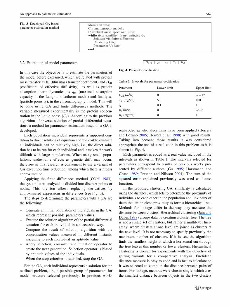
3.2 Estimation of model parameters

In this case the objective is to estimate the parameters of

the model before explained, which are related with protein

mass transfer as Ks (film mass transfer coefficient) and Deff

(coefficient of effective diffusivity), as well as protein

adsorption thermodynamics as qm (maximal adsorption

capacity in the Langmuir isotherm model) and finally ep

(particle porosity), in the chromatography model. This will

be done using GA and finite differences methods. The

variable measured experimentally is the protein concen-

tration in the liquid phase ðCbÞ: According to the previous

algorithm of inverse solution of partial differential equa-

tions, a method for parameters estimation based on a GA is

developed.

Each population individual represents a supposed con-

dition to direct solution of equation and the cost to evaluate

all individuals can be relatively high, i.e., the direct solu-

tion has to be run for each individual and it makes the work

difficult with large populations. When using small popu-

lations, undesirable effects as genetic drift may occur,

therefore in this research is convenient to use a variant of

GA execution time reduction, among which there is fitness

approximation.

Applying the finite differences method (ONeil 1983),

the system to be analyzed is divided into discreet points or

nodes. This division allows replacing derivatives by

approximated expressions in differences (see Fig. 3).

The steps to determinate the parameters with a GA are

the following:

– Generate an initial population of individuals in the GA,

which represent possible parameters values.

– Execute the solution algorithm of the partial differential

equation for each individual in a successive way.

– Compare the result of solution algorithm with the

concentration values measured in different instants,

assigning to each individual an aptitude value.

– Apply selection, crossover and mutation operator to

create the next generation. Selection operator is biased

by aptitude values of the individuals.

– When the stop criterion is satisfied, stop the GA.

For the GA, each individual represents a solution for the

outlined problem, i.e., a possible group of parameters for

model structure selected previously. In previous works

real-coded genetic algorithms have been applied (Herrera

and Lozano 2005; Herrera et al. 1998) with good results.

Taking into account those results it was considered

appropriate the use of a real code in this problem as it is

shown in Fig. 4.

Each parameter is coded as a real value included in the

intervals as shown in Table 1. The intervals selected for

parameters correspond to results of previous works pre-

sented by different authors (Gu 1995; Horstmann and

Chase 1989; Persson and Nilsson 2001). The sum of the

squared error explained previously was used as fitness

function.

In the proposed clustering GA, similarity is calculated

using the distance, which lets to determine the proximity of

individuals to each other in the population and link pairs of

them that are in close proximity to form a hierarchical tree.

Methods for linkage differ in the way they measure the

distance between clusters. Hierarchical clustering (Jain and

Dubes 1988) groups data by creating a cluster tree. The tree

is not a single set of clusters, but rather a multilevel hier-

archy, where clusters at one level are joined as clusters at

the next level. It is not necessary to specify previously the

maximum number of clusters. If it is set, the algorithm

finds the smallest height at which a horizontal cut through

the tree leaves this number or fewer clusters. Hierarchical

clustering is chosen for experiments with the objective of

getting variants for a comparative analysis. Euclidean

distance measure is easy to code and is fast to calculate so

it was selected to compute the distance between pairs of

items. For linkage, methods were chosen single, which uses

the smallest distance between objects in the two clusters

Fig. 3 Developed GA-based

parameter estimation method

Fig. 4 Parameter codification

Table 1 Intervals for parameter codification

Parameter Lower limit Upper limit

Deff (m2/s) 0 2e-12

qm (mg/ml) 50 100

ep 0.1 1

Ks (m/s) 0 2e-6

Kd (mg/ml) 0 1

An approach to parameters estimation 967

123

and Ward’s, that uses the sum of the squares of the dis-

tances between all objects in the cluster and the centroid of

the cluster. The first linkage tends to create big clusters and

therefore the number of individual evaluations would be

smaller, while the second is efficient although it can create

clusters of small size.

In the proposed clustering GA, a selection scheme by

means of two individual’s tournament was used. As

crossover operator the scattered uniform crossover was

applied. It creates a random binary vector and selects the

genes from the first parent if the bits in the vector are 1 or

from the second parent if the bits in the vector are 0. The

child is formed combining the genes. Because some

authors (Deb et al. 2002; Herrera et al. 2003) have pro-

posed advanced real-parameter crossover operators, many

experiments with different crossover operators were real-

ized later, but improvements were not obtained.

4 Experiments on synthetic data

The developed experiments and the obtained results using

synthetic data are presented in the first part of this section.

After that, a comparison between a simple GA and the

clustering GA is done.

4.1 Parameter study on clustering GA

For determination of GA, operation characteristics such as

crossover and mutation probabilities, population size and

stopping criterion have some practical criteria. It is nec-

essary to repeat the runs to test the GA performance in

different cases.

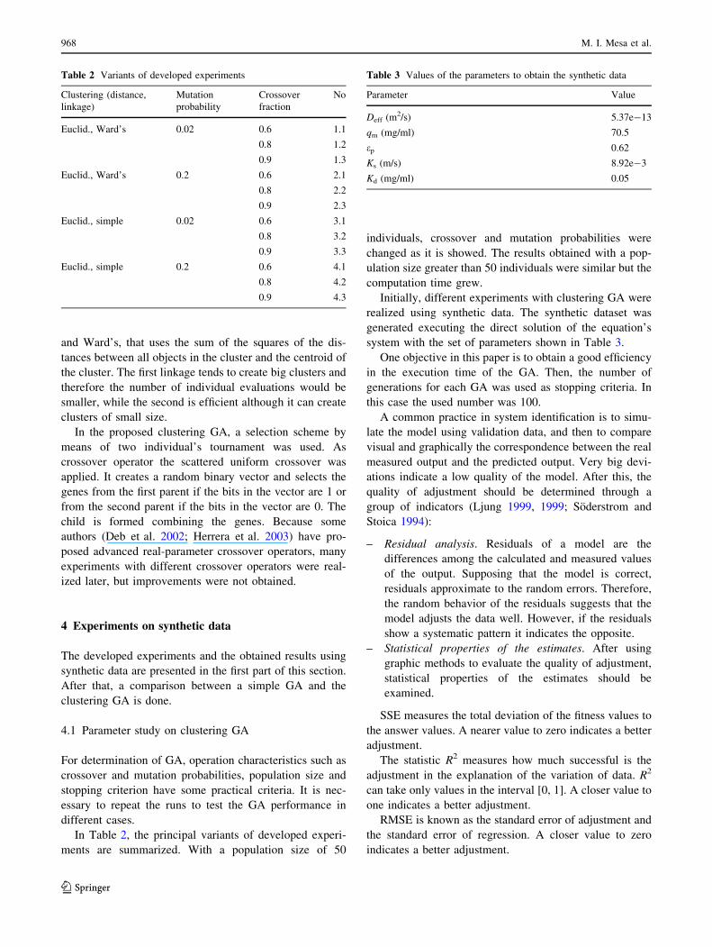
In Table 2, the principal variants of developed experi-

ments are summarized. With a population size of 50

individuals, crossover and mutation probabilities were

changed as it is showed. The results obtained with a pop-

ulation size greater than 50 individuals were similar but the

computation time grew.

Initially, different experiments with clustering GA were

realized using synthetic data. The synthetic dataset was

generated executing the direct solution of the equation’s

system with the set of parameters shown in Table 3.

One objective in this paper is to obtain a good efficiency

in the execution time of the GA. Then, the number of

generations for each GA was used as stopping criteria. In

this case the used number was 100.

A common practice in system identification is to simu-

late the model using validation data, and then to compare

visual and graphically the correspondence between the real

measured output and the predicted output. Very big devi-

ations indicate a low quality of the model. After this, the

quality of adjustment should be determined through a

group of indicators (Ljung 1999, 1999; Soderstrom and

Stoica 1994):

– Residual analysis. Residuals of a model are the

differences among the calculated and measured values

of the output. Supposing that the model is correct,

residuals approximate to the random errors. Therefore,

the random behavior of the residuals suggests that the

model adjusts the data well. However, if the residuals

show a systematic pattern it indicates the opposite.

– Statistical properties of the estimates. After using

graphic methods to evaluate the quality of adjustment,

statistical properties of the estimates should be

examined.

SSE measures the total deviation of the fitness values to

the answer values. A nearer value to zero indicates a better

adjustment.

The statistic R2 measures how much successful is the

adjustment in the explanation of the variation of data. R2

can take only values in the interval [0, 1]. A closer value to

one indicates a better adjustment.

RMSE is known as the standard error of adjustment and

the standard error of regression. A closer value to zero

indicates a better adjustment.

Table 2 Variants of developed experiments

Clustering (distance,

linkage)

Mutation

probability

Crossover

fraction

No

Euclid., Ward’s 0.02 0.6 1.1

0.8 1.2

0.9 1.3

Euclid., Ward’s 0.2 0.6 2.1

0.8 2.2

0.9 2.3

Euclid., simple 0.02 0.6 3.1

0.8 3.2

0.9 3.3

Euclid., simple 0.2 0.6 4.1

0.8 4.2

0.9 4.3

Table 3 Values of the parameters to obtain the synthetic data

Parameter Value

Deff (m2/s) 5.37e-13

qm (mg/ml) 70.5

ep 0.62

Ks (m/s) 8.92e-3

Kd (mg/ml) 0.05

968 M. I. Mesa et al.

123

Efficiency was calculated using the formula:

Efic ¼PT

t¼1 yðtÞ � yðtÞ� �2

�PT

t¼1 yðtÞ � yðtÞð Þ2

PTt¼1 yðtÞ � yðtÞ� �2

Another criterion to characterize the model is the calculus

of mean and variance of the real output, the estimated

output and the modeling error. It should be proven if a

correspondence exists among predictions given by the

model and experimental observations of the system. In that

case the estimated parameters are considered valid (Ljung

1999).

Table 4 shows statistical properties to allow a quanti-

tative comparison for 100 runs of the GA. Synthetic data

with a 3% of added random noise were used in these

experiments to simulate real data and assess the algorithm.

The results are the averages obtained in the 100 runs of

each experiment. In general, better results were reached

using Euclidean distance with Ward’s linkage for cluster-

ing and this demonstrate the validity of this method.

4.2 Clustering GA versus a simple GA and classic

methods

To compare simple and clustering GA respects to the mean

values of objective function and the execution time, some

experiments were developed. In those experiments the

same mutation and crossover operators and probabilities

values were used.

Table 5 shows the mean values of objective function

and execution time for ten runs of the GA in a CPU

Pentium 4, 2.4 GHz and 512 MB of RAM memory. In all

the cases the running times for the clustering GA are less

than for the simple GA. The clustering GA using Ward’s

linkage is slower than using single linkage, but the fitness

values are better in the first case. Best results are high-

lighted in boldface. The minimum running time for the

simple GA and the minimum fitness value are obtained

with 0.2 mutation probability and 0.9 crossover fraction.

In general, the combination of 0.2 mutation and 0.9

crossover fraction for the genetic operators yields satis-

factory results.

Table 4 Comparison of developed experiments results

Exp. num. Mean Standard deviation RMSE R2 Efic.

Meas. output Estim. output Error Meas. output Estim. output Error

1.1 0.2028 0.2023 0.0005 0.1575 0.1819 0.0244 0.0492 0.7517 0.9309

1.2 0.1955 0.2005 0.0050 0.1688 0.1761 0.0073 0.0303 0.9196 0.9721

1.3 0.2556 0.1979 0.0577 0.1466 0.1741 0.0275 0.0732 0.8199 0.8332

2.1 0.2085 0.2011 0.0074 0.1746 0.1764 0.0018 0.0311 0.9832 0.9706

2.2 0.1900 0.1994 0.0094 0.1715 0.1761 0.0046 0.0370 0.9738 0.9574

2.3 0.2133 0.2034 0.0099 0.1758 0.1778 0.0020 0.0300 0.9808 0.9730

3.1 0.2072 0.1998 0.0074 0.1758 0.1761 0.0003 0.0325 0.9991 0.9678

3.2 0.1933 0.2004 0.0071 0.1778 0.1838 0.0060 0.0347 0.9356 0.9663

3.3 0.2310 0.2034 0.0276 0.1338 0.1778 0.0440 0.0747 0.5909 0.8332

4.1 0.2212 0.2004 0.0208 0.1769 0.1838 0.0069 0.0400 0.9373 0.9552

4.2 0.2230 0.1998 0.0232 0.1670 0.1761 0.0091 0.0421 0.9153 0.9461

4.3 0.2055 0.2005 0.0050 0.1746 0.1761 0.0015 0.0275 0.9852 0.9770

Table 5 Comparative results of experiments with simple and clustering GA

Mut.

prob.

Cross.

fract.

Fitness GA

simple

Time GA(s)

simple

Fitness GA clust.

euclid., single

Time GA(s) clust.

euclid. single

Fitness clust.

euclid. ward

Time GA(s) clust.

euclid., ward

0.02 0.6 8.33e-4 92.26 4.59e-4 25.22 8.64e-4 39.85

0.8 1.00e-3 92.98 1.33e-2 24.78 2.42e-2 36.78

0.9 1.10e-3 100.97 0.27e-2 26.87 7.82e-2 35.84

0.2 0.6 1.11e24 134.30 1.54e-2 24.75 2.41e-4 37.01

0.8 3.30e-4 92.39 0.16e-2 24.40 6.72e-4 36.15

0.9 3.74e-4 91.06 1.06e24 24.43 9.41e25 36.09

An approach to parameters estimation 969

123

Results of experiments with some classic methods

aforementioned are shown in Table 6. In these experi-

ments, initial values in the algorithms runs were set as the

minimum typical values for the parameters to be estimated.

It is evident that the results for clustering GA experiments

shown in Table 5 are better than the results with classic

algorithms in all the cases.

Non-parametric tests could be applied to small sample

of data and their effectiveness have been proved in com-

plex experiments. Wilcoxon signed-rank test is a non-

parametric statistical procedure for performing pairwise

comparisons between two algorithms (Garcia et al. 2009).

In the null hypothesis H0 the average rank of the results are

equal. In the alternative hypothesis H1 there is a difference.

The ranks are computed as follows:

Rþ ¼X

di [ 0

rankðdiÞ þ1

2

X

di¼0

rankðdiÞ

R� ¼X

di\0

rankðdiÞ þ1

2

X

di¼0

rankðdiÞ;

where di is the difference between the performance of the

two algorithms on the i-th run. These differences are sorted

in an upward way and the ranks are computed accordingly.

If the smallest of the sums, T ¼ minðRþ;R�Þ is less than or

equal to the value of the distribution of Wilcoxon for

N degrees of freedom (Zar 1999) the null hypothesis of

equality is rejected.

In this case it is used to compare the results between the

behavior of simple and clustering genetic algorithms and to

stipulate which one is the best with a probability of error,

that is the complement of the probability of reporting that

two systems are the same, called the p value (Zar 1999).

The computation of the p value in the Wilcoxon distribu-

tion could be carried out by computing a normal approxi-

mation (Sheskin 1736).

Table 7 shows the results obtained in the comparisons,

being R? the sum of the ranks for which the clustering GA

outperformed the simple GA. These ranks were computed

Table 6 Results of experiments with classic methods

Algorithm Objective function

evaluation

Time

(s)

Broydon–Fletcher–Goldfarb–Shanno

(BFGS)

0.0499 218.78

Nelder–Mead 0.0134 180.65

Levenberg–Marquardt 0.0062 173.25

Gauss–Newton 0.0528 173.32

Table 7 Wilcoxon test results

Mut. prob. Cross. fract. Euclid. single Euclid. ward

R? R- p value R? R- p value

0.02 0.6 4,066 29 4.5926e-16 4,095 0 1.7438e-16

0.8 4,095 0 1.7438e-16 2,251 1,844 0.4129

0.9 4,095 0 1.7438e-16 4,093 2 1.865e-16

0.2 0.6 4,095 0 1.7438e-16 3,553 542 1.3811e-9

0.8 2,826 1,269 0.0017 4,095 0 1.7438e-16

0.9 4,095 0 1.7438e-16 4,095 0 1.7438e-16

Error

-0.04

-0.02

0

0.02

0.04

0.06

time (min)

time (min)

Cb (t)

C0

C0= 2.5 mg/mL

0 20 40 60 80 100 120 140 160 180

0 20 40 60 80 100 120 140 160 180

0.4

0.5

0.6

0.7

0.8

0.9

1

- realx estimate

0.08

Fig. 5 Estimated output and error values corresponding to the

solution determined by GA for an initial concentration value of

2.5 mg/ml

970 M. I. Mesa et al.

123

from the difference of errors obtained evaluating the direct

solution of the model for mean values of the estimated

parameters in ten runs of the clustering and simple GA,

respectively, and considering 90 samples. With the

exception of the value highlighted in boldface, the rest are

valid and better for clustering GA performance. As can be

seen, in all of the experiments where Euclidean distance

and Ward’s linkage was applied, the clustering GA was the

winner algorithm.

5 Validation of the results using real data: a case study

on the adsorption of proteins in macro porous solid

for chromatography in stirred tank

Parameters values were identified for ten runs of the GA

with equal operation characteristics and for each datasets

corresponding to three different initial concentrations val-

ues aforementioned.

Samples of concentration were acquired every 2 min,

for a total of 90, which were used out of line to test the

algorithm runs.

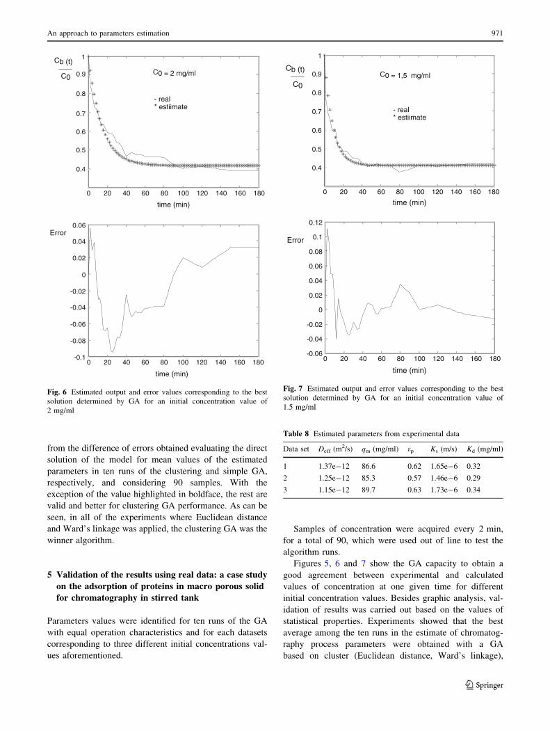
Figures 5, 6 and 7 show the GA capacity to obtain a

good agreement between experimental and calculated

values of concentration at one given time for different

initial concentration values. Besides graphic analysis, val-

idation of results was carried out based on the values of

statistical properties. Experiments showed that the best

average among the ten runs in the estimate of chromatog-

raphy process parameters were obtained with a GA

based on cluster (Euclidean distance, Ward’s linkage),

Cb (t)

C0

0 20 40 60 80 100 120 140 160 180

0.4

0.5

0.6

0.7

0.8

0.9

1

time (min)

- real* estiimate

C0 = 2 mg/ml

Error

0 20 40 60 80 100 120 140 160 180-0.1

-0.08

-0.06

-0.04

-0.02

0

0.02

0.04

0.06

time (min)

Fig. 6 Estimated output and error values corresponding to the best

solution determined by GA for an initial concentration value of

2 mg/ml

0 20 40 60 80 100 120 140 160 180

0.4

0.5

0.6

0.7

0.8

0.9

1

Error

0 20 40 60 80 100 120 140 160 180-0.06

-0.04

-0.02

0

0.02

0.04

0.06

0.08

0.1

0.12

time (min)

time (min)

- real* estiimate

C0 = 1,5 mg/mlCb (t)

C0

Fig. 7 Estimated output and error values corresponding to the best

solution determined by GA for an initial concentration value of

1.5 mg/ml

Table 8 Estimated parameters from experimental data

Data set Deff (m2/s) qm (mg/ml) ep Ks (m/s) Kd (mg/ml)

1 1.37e-12 86.6 0.62 1.65e-6 0.32

2 1.25e-12 85.3 0.57 1.46e-6 0.29

3 1.15e-12 89.7 0.63 1.73e-6 0.34

An approach to parameters estimation 971

123

non-uniform mutation operator with mutation probability

equal to 0.2 and scattered crossover with a probability

equal to 0.9. The values of estimated parameters for this

case are shown in Table 8. These GA parameters together

with generation number of 100 and population size of 50

can be used as starting point for further experiments of

parameters estimation in similar chromatographic

processes.

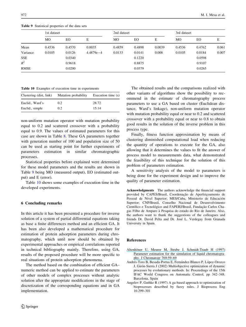
Statistical properties before explained were determined

for these model parameters and the results are shown in

Table 9 being MO (measured output), EO (estimated out-

put) and E (error).

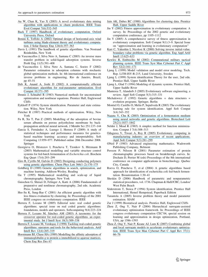
Table 10 shows some examples of execution time in the

developed experiments.

6 Concluding remarks

In this article it has been presented a procedure for inverse

solution of a system of partial differential equations taking

as base a finite differences method and an efficient GA. It

has been also developed a mathematical procedure for

estimation of protein adsorption parameters during chro-

matography, which until now should be obtained by

experimental approaches or empirical correlations reported

in technical bibliography mainly. Therefore, using GA,

results of the proposed procedure will be more specific to

real situations of protein adsorption phenomena.

The method based on the combination of efficient GA–

numeric method can be applied to estimate the parameters

of other models of complex processes without analytic

solution after the appropriate modifications in the stage of

discretization of the corresponding equations and in GA

implementation.

The obtained results and the comparisons realized with

other variants of algorithms show the possibility to rec-

ommend in the estimate of chromatography process

parameters to use a GA based on cluster (Euclidean dis-

tance, Ward’s linkage), non-uniform mutation operator

with mutation probability equal or near to 0.2 and scattered

crossover with a probability equal or near to 0.8 to obtain

good results in the solution of the inverse problem in this

process type.

Finally, fitness function approximation by means of

clustering diminished computational load when reducing

the quantity of operations to execute for the GA, also

allowing that it determines the values to fit the answer of

process model to measurements data, what demonstrated

the feasibility of this technique for the solution of this

problem of parameters estimation.

A sensitivity analysis of the model to parameters is

being done for the experiment design and to improve the

quality of parameter estimation.

Acknowledgments The authors acknowledge the financial support

provided by CAPES/Brasil, Coordenacao de Aperfeicoamento de

Pessoal de Nıvel Superior; MES/Cuba, Ministerio de Educacion

Superior; CNP/Brasil, Conselho Nacional de Desenvolvimento

Cientıfico e Tecnologico and FAPERJ/Brasil, Fundacao Carlos Cha-

gas Filho de Amparo a Pesquisa do estado do Rio de Janeiro. Also,

the authors want to thank the suggestions of the colleagues and

friends Dr. David Pelta and Dr. Jose L. Verdegay from Granada

University in Spain.

References

Altenhoner U, Meurer M, Strube J, Schmidt-Traub H (1997)

Parameter estimation for the simulation of liquid chromatogra-

phy. J Chromatogr 769:59–69

Andres-Toro B, Besada-Portas E, Fernandez-Blanco P, Lopez-Orozco

J, Giron-Sierra J (2002) Multiobjective optimization of dynamic

processes by evolutionary methods. In: Proceedings of the 15th

IFAC World Congress on Automatic Control, pp 342–348.

Barcelona, Spain

Angelov P, Guthke R (1997) A ga-based approach to optimization of

bioprocesses described by fuzzy rules. J Bioprocess Eng

16:299–301

Table 9 Statistical properties of the data sets

1st dataset 2nd dataset 3rd dataset

MO EO E MO EO E MO EO E

Mean 0.4536 0.4570 0.0035 0.4859 0.4898 0.0039 0.4536 0.4762 0.061

Variance 0.0105 0.0126 4.4879e-4 0.0133 0.0141 0.008 0.0105 0.0184 0.007

SSE 0.0340 0.1220 0.0598

R2 0.9618 0.8875 0.9107

RMSE 0.0200 0.0379 0.0265

Table 10 Examples of execution time in experiments

Clustering (dist, link) Mutation probability Execution time (s)

Euclid., Ward’s 0.2 28.72

Euclid., simple 0.2 15.14

972 M. I. Mesa et al.

123

Au W, Chan K, Yao X (2003) A novel evolutionary data mining

algorithm with applications to churn prediction. IEEE Trans

Evol Comput 7(6):532–545

Back T (1997) Handbook of evolutionary computation. Oxford

University Press, Oxford

Benini E, Toffolo A (2002) Optimal design of horizontal-axis wind

turbines using blade-element theory and evolutionary computa-

tion. J Solar Energy Eng 124(4):357–363

Davis L (1991) The handbook of genetic algorithms. Van Nostrand

Reinholdm, New York

de Vasconcellos J, Silva Neto A, Santana C (2003) An inverse mass

transfer problem in solid-liquid adsorption systems. Inverse

Probl Eng 11(5):391–408

de Vasconcellos J, Silva Neto A, Santana C, Soeiro F (2002)

Parameter estimation in adsorption columns with stochastic

global optimization methods. In: 4th international conference on

inverse problems in engineering, Rio de Janeiro, Brazil,

pp 45–51

Deb K, Anand A, Joshi D (2002) A computationally efficient

evolutionary algorithm for real-parameter optimization. Evol

Comput 10:371–395

Dennis J, Schnabel R (1983) Numerical methods for unconstrained

optimization and nonlinear equations. Prentice Hall, Englewood

Cliffs

Eykhoff P (1974) System identification. Parameter and state estima-

tion. Wiley, New York

Fletcher R (1987) Practical methods of optimization. Wiley, New

York

Fu R, Xu T, Pan Z (2005) Modelling of the adsorption of bovine

serum albumin on porous polyethylene membrane by back-

propagation artificial neural network. J Membr Sci 251:137–144

Garcia S, Fernandez A, Luengo J, Herrera F (2009) A study of

statistical techniques and performance measures for genetics-

based machine learning: accuracy and interpretability. Soft

Computing 13:959–977. Published online 20th December 2008.

Springer

Georgieva O, Hristozov I, Pencheva T, Tzonkov S, Hitzmann B

(2003) Mathematical modelling and variable structure control

systems for fed-batch fermentation of Escherichia coli. Biochem

Eng Quart 17(4):293–299

Giro R, Cyrillo M, Galvao D (2002) Designing conducting polymers

using genetic algorithms. Chem Phys Lett 366(1–2):170–175

Goldberg D (1989) Genetic algorithms in search, optimization, and

machine learning. Addison-Wesley, Reading

Gu T (1995) Mathematical modelling and scale-up of liquid

chromatography. Springer, New York

Guiochon G, Shirazi D, Felinger A, Katti A (2006) Fundamentals of

preparative and nonlinear chromatography, 2nd edn. Academic

Press, London

Hee-Su K, Sung-Bae C (2001) An efficient genetic algorithm with

less fitness evaluation by clustering. In: Proceedings of the 2001

IEEE congress on evolutionary computation. IEEE

Herrera F, Lozano M (2005) Editorial note: real coded genetic

algorithms. special issue on real coded genetic algorithms:

foundations, models and operators. Softcomputing 9(4):223–224

Herrera F, Lozano M, Sanchez AM (2003) A taxonomy for the

crossover operator for real-coded genetic algorithms. an exper-

imental study. Int J Intell Syst 18(3):309–338

Herrera F, Lozano M, Verdegay J (1998) Tackling real-coded genetic

algorithms: operators and tools for the behavioral analysis. Artif

Intell Rev 12(4):265–319

Horstmann BJ, Chase HA (1989) Modelling the affinity adsorption of

immunoglobulin g to protein a immobilized to agarose matrices.

Chem Eng Res Des 67

Jain AK, Dubes RC (1988) Algorithms for clustering data. Prentice

Hall, Upper Saddle River

Jin Y (2002) Fitness approximation in evolutionary computation: A

survey. In: Proceedings of the 2002 genetic and evolutionary

computation conference, pp 1105–1112

Jin Y (2005) A comprehensive survey of fitness approximation in

evolutionary computation. Soft Comput 9(1):3–9. Special Issue

on ‘‘approximation and learning in evolutionary computation’’

Karr C, Yakushin I, Nicolosi K (2000) Solving inverse initial-value,

boundary-value problems via genetic algorithm. Eng Appl Artif

Intell 13:625–633

Kewley R, Embrechts M (2002) Computational military tactical

planning system. IEEE Trans Syst Man Cybernet Part C Appl

Rev 32(2):161–171

Ljung L (1999) Model validation and model error modeling. Tech.

Rep. LiTH-ISY-R-215, Lund University, Sweden

Ljung L (1999) System identification Theory for the user, 2nd edn.

Prentice Hall, Upper Saddle River

Ljung L, Glad T (1994) Modeling of dynamic systems. Prentice Hall,

Upper Saddle River

Manterea T, Alanderb J (2005) Evolutionary software engineering, a

review. Appl Soft Comput 5(3):315–331

Michalewicz Z (1992) Genetic algorithms ? data structures =

evolution programs. Springer, Berlin

Montiel O, Castillo O, Melin P, Sepulveda R (2003) The evolutionary

learning rule for system identification. Appl Soft Comput

3(4):343–352

Nagata Y, Chu K (2003) Optimization of a fermentation medium

using neural networks and genetic algorithms. Biotechnol Lett

25(21):1837–1842

Nelder J, Mead R (1965) A simplex method for function minimiza-

tion. Comput J 7(4):308–313

Oduguwa V, Tiwari A, Roy R (2005) Evolutionary computing in

manufacturing industry: an overview of recent applications.

Appl Soft Comput 5(3):281–299

ONeil P (1983) Advanced engineering mathematics. Wadsworth

Publishing Company, Belmont

Persson P, Nilsson B (2001) Parameter estimation of protein

chromatographic processes based on breakthrough curves. In:

Dochain D, Perrier M (eds) Proceedings of the 8th international

conference on computer applications in biotechnology. Quebec

City, Canada

Roeva O, Pencheva T, et al (2004) A genetic algorithms based

approach for identification of escherichia coli fed-batch fermen-

tation. Bioautomation 1:30–41

Sheskin D (2006) Handbook of parametric and nonparametric

statistical procedures, vol. 1736. Chapman & Hall//CRC, Londos/

West Palm Beach

Soderstrom T, Stoica P (1994) System identification. Prentice Hall

International, Hemel Hempstead, Paperback Edition

Tarantola A (2005) Inverse problem theory and model parameter

estimation. SIAM

Zar J (1999) Biostatiscal analysis. Prentice Hall, Englewood Cliffs

Zhou Z, Ong Y, Nair P (2004) Hierarchical surrogate-assisted

evolutionary optimization framework. In: Proceedings of IEEE

congress evolutionary computation CEC’04, special session on

learning and approximation in design optimization, Portland,

USA, pp 1586–1593

Zhou Z, Ong Y, Nair P, Keane AJ, Lum K (2007) Combining global

and local surrogate models to accelerate evolutionary optimiza-

tion. IEEE Trans Syst Man Cybernet Part C Appl Rev 37(1):

66–76

An approach to parameters estimation 973

123