An Application to Ebola Type Infectious Disease - Letters in ...

LETTERS IN BIOMATHEMATICSAn International Journal

RESEARCH ARTICLE OPEN ACCESS

Modeling Assumptions, Mathematical Analysis andMitigation Through Intervention: An Application to EbolaType Infectious Disease

Ram Singh,a Naveen Sharma,a Aditi Ghoshb

aDepartment of Mathematical Sciences, BGSB University, Rajouri 185234, J&K, (India); bDepartment of Mathematics,University of Wisconsin-Whitewater, USA

ABSTRACTEbola virus is a life-threatening virus and has two major characteristics; one potentialto have high mortality rate and the other infection transmission through newlyinfected dead bodies. There are some relevant features of Ebola that were observedduring its recent outbreak: including varying rate of access to isolation facilities bypatients and transmission of infection via improper handling of the dead bodies ofinfected diseased. Quick and safe burial may play an important role in the controland prevention of this virus. In this study, we consider mathematical modelingframework with four different cases for dynamics of Ebola virus with safe and unsafeburial practices, vaccination and treatment interventions with varying efficiency. Thegoal of this study is to show how timely treatment to Ebola leads to an effectivecontrol of the virus and, most importantly, how safe burial of dead bodies helpscontrol the spread.

ARTICLE HISTORYReceived November 27, 2018Accepted December 18, 2019

KEYWORDSEbola virus, dead bodies,stability analysis, Lyapunovfunctional

1 IntroductionEbola virus is one of the virulent viruses that frequently emerges in both developing and developed nations and is a matter ofserious concern for the entire world because of its high fatality ratio (WHO, 2014a; Summers et al., 2015). One of the transmis-sions of this disease is through body uids of infected or dead humans or animals. Also, for this deadly virus disease, no eectivedrug has yet been discovered. Many researchers and biologists have conducted studies to understand the transmission dynam-ics and control of the disease but still not much is understood as to how to control the spread of this disease eectively. As peravailable literature, rst case of Ebola virus (EV) outbreakswith documentation evidence detected in 1976 (Rathore et al., 2014).Hemorrhagic fever, normally known as Ebola virus disease (EVD), is taken to be the case that commenced in themid-seventies inGuinea (Feldmann andGeisbert, 2011; Feldmann et al., 2003; Kortepeter et al., 2011). Due to this contingency, 3000 conditionsand 1500 deceases were sustained in Guinea, Liberia, Nigeria and Sierra Leone. Considering these inventive conditions, therewere more or less 20 major episodes through the year 2014 (CDC, 2014). The latest events which started in Guinea at the early2014 and after that spread to Liberia and Sierra Leone, is the longest, largest and most widespread Ebola event. Therefore onAugust 8, 2014, WHO announced the epidemic to be a Public Health Emergency of International Concern (PHEIC) (WHO,2014b). In accordance with the WHO report, as of Nov. 2, 2014, a total of 13,042 suspected cases and 4,818 armed deathswere registered. Amongst these dying, 4,791 (approx. 99.5%) were diagnosed inWest African countries (CDC, 2014). The newbroad expanded conicts of EVD in Western Africa was due to Bundibugyo Ebola virus and Sudan Ebola virus, particularlythe present conict of 2014 is an attribute to the Zaire species (Du Toit, 2014). Ebola virus normally gets transmitted into thehuman population through close contact with blood, secretions, organs or other body uids of infected animals such as chim-panzees, gorillas, fruit-bats, monkeys, forest antelope and porcupines found ill or dead in the rainforest. Countries like WestAfrica and South Asia are at high risk of Ebola virus. The main symptoms of Ebola virus such as fever fatigue muscular pain,vomiting, diarrhoea, can be seen within four to six days after a person becomes infected with this harmful disease. Due to nonavailability of antiviral drug for this deadly virus it is dicult to control the spread of this disease. However, early stage treatmentas the symptoms of virus appears in human, basic interventions can signicantly improve the chances of survival which include:

CONTACT Aditi Ghosh [email protected] Lett. Biomath., Vol. 6, Iss. 2 (2019), pp. 1–19.

2 R. SINGH, N. SHARMA, A. GHOSH

giving more uid and electrolytes through injection, supplying oxygen to balance the oxygen level and appropriate medicinelike ZMapp and rVSV-ZEBOV for early treatment. In a recent experiment, it has been found that nucleoside analogue- andsiRNA-based therapies are very much eective if a therapy with a > 50% controlling rate is administrated within a few dayspost-symptom-onset (Martyushev et al., 2016). Eective drugs play very a vital role in controlling the dynamics of Ebola virus.It has been worth mentioning that many times the symptoms of Ebola infection are mistaken by other disease like dengue feverand other infectious diseases. The spread of Ebola virus poses a threat to many countries because the location and identicationof the virus is still unknown (Madubueze et al., 2018).

Over the past years, several mathematical models have been proposed and developed to describe the dynamics of Ebola virus(EV) (Kabli et al., 2018; Singh et al., 2016; Althaus, 2014; Legrand et al., 2007; Mubayi et al., 2010; Wang and Zhong, 2015;Rachah and Torres, 2015, 2016, 2017; Chowell et al., 2004; Grigorieva and Khailov, 2014; Area et al., 2015; Jones, 2017; Xiaet al., 2015; Zhu et al., 2016). Agusto (2017) developed a mathematical model which exhibits that the infection in Ebola virus isrecurrence based. A recent new generalized epizootic model that describes the transmission dynamics of Ebola virus disease inbat population is main reservoir of the Ebola virus (EL Rhoubari et al., 2018; Jiang et al., 2017; Yusuf and Benyah, 2012; Huoand Feng, 2013; LaSalle, 1976; Feng andVelasco-Hernández, 1997; Abdelrazec et al., 2016; Singh et al., 2019; Singh and Sharma,2018; Singh et al., 2018, 2010). Recently, many othermathematical models have been formulated and studied (Ullah et al., 2019;Khan et al., 2019; Ahmad et al., 2019) to understand the transmission dynamics of many human killing diseases which is stillchallenging and are open threat to medical practitioners.

Another aspect of studymodelling of epidemics is to nd an optimal solution of various problems. Mathematicalmodellingregarding the epidemics such as zika virus and hepatitis B virus etc. with optimal control solutions have intensively studied byWasim et al. (2019) and Ullah et al. (2019). The main contribution of this paper is to study the dynamical behaviour of thetransmission dynamics of Ebola virus in the treatment class which are not mentioned in earlier work. Weitz andDusho (2015)particularly show in their work that reduction in transmission risk after death can have substantial epidemiological benets. Theidentiability problem relevant to EVD is addressed in his work and shows that improved estimation of post death transmis-sion would help control the spread of the disease and improve reliability in estimates of reproductive number. In the work ofNielsen et al. (2015) improvement of burial practices and cemetery management has been addressed to control the spread ofEVD eectively.

In this paper, a mathematical model for the dynamics of Ebola virus with safe burial of disease dead bodies is proposedand analyzed to know the primary facts and information about the Ebola virus. Ebola virus spreads by touching the bodies ofperson who died of ebola disease. To prevent this infection, it is mandatory to make safe burial of the dead bodies (Weitz andDusho, 2015). The safe burial of those who have died of Ebola is acknowledged as an important intervention for controllingepidemics. Ebola virus spreads mainly through human to human transmission via direct contact with blood or body uids ofa person who is sick with or has died from Ebola and objects that have been contaminated with body uids (like blood, feces,vomit) from a person sick with Ebola or the body of a person who died from Ebola. Health-care workers have frequently beeninfectedwhile treating patients with suspected or conrmed Ebola virus (EVD). This occurs through close contact with patientswhen infection control precautions are not strictly practiced. Safe burial ceremonies that involve direct contact with the bodyof the deceased can also contribute in the transmission of Ebola. It has been observed that in absence of medicine and vaccines,early diagnosis, isolation of suspected, awareness campaigns and sanitary burial practices are eective controls to stop diseasespread (Diekmann et al., 1990; Chowell et al., 2015; Chowell and Nishiura, 2014; Dhillon et al., 2015; Feng et al., 2000). Weconsider four dierentmathematical models with dierent rates to understand the dynamics of this deadly virus with safe burialof its deaths as we consider safe burial as one of the major controlling strategies. In this paper, our primary target is to build arobust mathematical model to get insight about the impact of recovery rate and study the eect of limited resources on diseasesand how safe burial is important in controlling the diseases. It also provide insights where prevention and control interventionscould be targeted in future.

The organization of this paper is as follows. Section2presents themathematical description of the proposed dierentmodel.Section 3 provides the detailed analysis for all possible cases. Numerical results and simulation are carried out in Section 4.Section 5 is devoted to discussion. The conclusion is drawn in Section 6.

2 Model Description: Capturing transmission dynamics of Ebola virusThemodeling population is divided into six categories based on infection status (the denition of categories is given in Table 2).The total humanpopulation at time t is givenby,N (t) = A(t)+B(t)+C (t)+D(t)+E(t)+F (t), where susceptible is representedby A, infected classes by B, C and D, treatment class as E, and removed class (that includes recovered individuals and disease-related deaths) is represented by F . Susceptible population is increased by the recruitment of individuals into the populationat a rate Λ, through birth and net migration. The description of other parameters is provided in Table 3. The infected state isfurther sub-divided into three classes: asymptomatic class, symptomatic and severely infected with Ebola class. Individuals candie via natural causes or due to disease. It is further assumed that the treatments are given to symptomatic and severely infected

LETTERS IN BIOMATHEMATICS 3

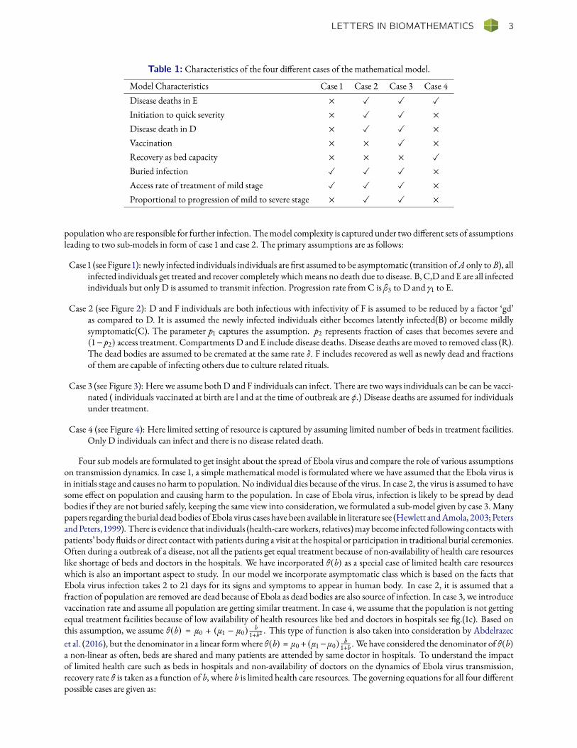
Table 1: Characteristics of the four dierent cases of the mathematical model.

Model Characteristics Case 1 Case 2 Case 3 Case 4Disease deaths in E × X X X

Initiation to quick severity × X X ×Disease death in D × X X ×Vaccination × × X ×Recovery as bed capacity × × × X

Buried infection X X X ×Access rate of treatment of mild stage X X X ×Proportional to progression of mild to severe stage × X X ×

populationwho are responsible for further infection. Themodel complexity is captured under two dierent sets of assumptionsleading to two sub-models in form of case 1 and case 2. The primary assumptions are as follows:

Case 1 (see Figure 1): newly infected individuals individuals are rst assumed to be asymptomatic (transition ofA only toB), allinfected individuals get treated and recover completely whichmeans no death due to disease. B, C,D and E are all infectedindividuals but only D is assumed to transmit infection. Progression rate from C is β3 to D and γ1 to E.

Case 2 (see Figure 2): D and F individuals are both infectious with infectivity of F is assumed to be reduced by a factor ‘gd’as compared to D. It is assumed the newly infected individuals either becomes latently infected(B) or become mildlysymptomatic(C). The parameter p1 captures the assumption. p2 represents fraction of cases that becomes severe and(1− p2) access treatment. Compartments D and E include disease deaths. Disease deaths are moved to removed class (R).The dead bodies are assumed to be cremated at the same rate δ. F includes recovered as well as newly dead and fractionsof them are capable of infecting others due to culture related rituals.

Case 3 (see Figure 3): Here we assume bothD and F individuals can infect. There are two ways individuals can be can be vacci-nated ( individuals vaccinated at birth are l and at the time of outbreak are ϕ.) Disease deaths are assumed for individualsunder treatment.

Case 4 (see Figure 4): Here limited setting of resource is captured by assuming limited number of beds in treatment facilities.Only D individuals can infect and there is no disease related death.

Four sub models are formulated to get insight about the spread of Ebola virus and compare the role of various assumptionson transmission dynamics. In case 1, a simple mathematical model is formulated where we have assumed that the Ebola virus isin initials stage and causes no harm to population. No individual dies because of the virus. In case 2, the virus is assumed to havesome eect on population and causing harm to the population. In case of Ebola virus, infection is likely to be spread by deadbodies if they are not buried safely, keeping the same view into consideration, we formulated a sub-model given by case 3. Manypapers regarding the burial dead bodies of Ebola virus cases have been available in literature see (Hewlett andAmola, 2003; PetersandPeters, 1999). There is evidence that individuals (health-careworkers, relatives)maybecome infected following contactswithpatients’ body uids or direct contact with patients during a visit at the hospital or participation in traditional burial ceremonies.Often during a outbreak of a disease, not all the patients get equal treatment because of non-availability of health care resourceslike shortage of beds and doctors in the hospitals. We have incorporated θ(b) as a special case of limited health care resourceswhich is also an important aspect to study. In our model we incorporate asymptomatic class which is based on the facts thatEbola virus infection takes 2 to 21 days for its signs and symptoms to appear in human body. In case 2, it is assumed that afraction of population are removed are dead because of Ebola as dead bodies are also source of infection. In case 3, we introducevaccination rate and assume all population are getting similar treatment. In case 4, we assume that the population is not gettingequal treatment facilities because of low availability of health resources like bed and doctors in hospitals see g.(1c). Based onthis assumption, we assume θ(b) = µ0 + (µ1 − µ0) b

1+b2 . This type of function is also taken into consideration by Abdelrazecet al. (2016), but the denominator in a linear formwhere θ(b) = µ0+ (µ1−µ0) b

1+b . We have considered the denominator of θ(b)a non-linear as often, beds are shared and many patients are attended by same doctor in hospitals. To understand the impactof limited health care such as beds in hospitals and non-availability of doctors on the dynamics of Ebola virus transmission,recovery rate θ is taken as a function of b, where b is limited health care resources. The governing equations for all four dierentpossible cases are given as:


Case 1: Model without disease induced death rate (δ = 0)

dA

dt= Λ −

β1AD

N+ σF − µA

dD

dt= β3C − (µ + γ)D

dB

dt=β1AD

N− (β2 + µ)B

dE

dt= γ1C + γD − (µ + θ)E

dC

dt= β2B − (β3 + µ + γ1)C

dF

dt= θE − (σ + µ)F

(1)

Case 2: Model with disease induced death rate

dA

dt= Λ −

β1A(D + gdF )N

+ σF − µAdD

dt= p2β3C − (µ + γ + δ)D

dB

dt= p1

β1A(D + gdF )N

− (β2 + µ)BdE

dt= (1 − p2)β3C + γD − (µ + θ + δ)E

dC

dt= β2B − (β3 + µ)C + (1 − p1)

β1A(D + gdF )N

dF

dt= θE − (σ + µ)F + δD + δE − δF

(2)

Case 3: Model with vaccination rate φ

dA

dt= Λ(1 − l) −

β1A(D + gdF )N

+ σF − µA − φAdD

dt= p2β3C − (µ + γ + δ)D

dB

dt= p1

β1A(D + gdF )N

− (β2 + µ)BdE

dt= (1 − p2)β3C + γD − (µ + θ + δ)E

dC

dt= β2B − (β3 + µ)C + (1 − p1)

β1A(D + gdF )N

dF

dt= Λl + θE − (σ + µ)F + δD + δE − δF + φA

(3)

Case 4: Model with recovery rate as a special function of θ(b)

dA

dt= Λ −

β1AD

N+ σF − µA

dD

dt= β3C − (µ + γ)D

dB

dt=β1AD

N− (β2 + µ)B

dE

dt= γ1C + γD − (µ + θ(b))E

dC

dt= β2B − (β3 + µ + γ1)C

dF

dt= θ(b)E − (σ + µ)F

(4)

Figure 1: Flow diagram of Ebola virus among dierent compartments for case 1.


Table 2: Dierent compartment along with their description used in models in all four cases.

Compartment DescriptionA(t) Number of Susceptible individuals who can get EbolaB(t) Number of individuals who are latently infected and are asymptomaticC (t) Mildly Symptomatic individuals who are non-infectious and may receive treatment for EbolaD(t) Number of severely symptomatic individuals who are infectiousE(t) Number of Individuals under treatment and are isolatedF (t) Removed individuals that includes recovered cases disease related deaths

(assumed dead bodies may be able to spread infection after death)

Table 3: Parameters and variables used in all models.

Parameters Denitions Value Source

Λ per capita recruitment rate of the population 0.55 years−1 Assumed(newly recruited individuals are assumed to be susceptible)

γ1, γ per capita rate of transition from C and D respectively 0.178 Chowell et al., 2015

p1 proportion of infected individuals that are asymptomatic 0.35 Assumed

p2 fraction of mildly symptomatic individuals that become 0.15 Assumedseverely infected

β1 transmission coecient from infected to susceptible 0.03 years−1 Chowell et al., 2015

β2 per capita progression rate from asymptomatic to 0.15 years−1 Diekmann et al., 1990mildly symptomatic

β3 per capita transition rate of patients from 0.35 years−1 Diekmann et al., 1990mildly symptomatic to severely infected

θ recovery rate per capita 0.03 years−1 Diekmann et al., 1990

δ diseases induced death rate per capita 0.0001 years−1 Diekmann et al., 1990

δ removal rate of disease deaths per capita 0.0002 years−1 Assumed

µ natural death rate per capita 0.0196 years−1 Diekmann et al., 1990

σ per capita loosing rate of temporary recovery Variable

φ vaccination rate at older ages 0.4 Assumed

g fraction of dead bodies that can generate new infection 0.5 Assumed

d fraction of g F that are not safely buried 0.5 Assumed

l proportion of individuals that are vaccinated at birth 0.4 Assumed

µ0 minimum recovery rate per capita 0.1 years−1 Carr, 2012

µ1 maximum recovery rate per capita 10 years−1 Carr, 2012

b fraction of health care resources available 0.20 Carr, 2012


3 The AnalysisBounded and Invariant Region

Tomake our system (1)–(4) biologically meaningful, it is necessary to show the positivity and boundedness of the solutions.

Lemma 3.1 The feasible regionΩ defined by

Ω ={(A(t),B(t),C (t),D(t),E(t), F (t)

)∈ R6

+ : N (t) ≤ Λµ

}with initial conditions A(t) ≥ 0, B(t) ≥ 0, C (t) ≥ 0, D(t) ≥ 0, E(t) ≥ 0, F (t) ≥ 0 is positively invariant for system ofequations (1)–(4).

Proof. Adding the equations of system (1)–(4), we obtain

dN

dt≤ Λ − µN . (5)

Solving this dierential equation (5), we have

0 ≤ N (t) ≤ Λ

µ+N (0)e−µt

where N (0) represents the initial values of the total population. Thus lim supt→+∞N (t) ≤ Λµ . It implies that the region

Ω ={(A(t),B(t),C (t),D(t),E(t), F (t)

)∈ R6

+ : N (t) ≤ Λµ

}is a positively invariant set for system (1)–(4). So existence and

uniqueness of system (1)–(4) on the region given by setΩ. �

3.1 Case 1 AnalysisIn this section we derive the equilibrium states and investigate their stability by using the reproduction number. Dynamicalsystem (1)–(4) has disease-free equilibrium given by,

E0 =(A0, B0, C0, D0, E0, F 0) = (

Λµ , 0, 0, 0, 0, 0

).

The basic reproduction number, <0 is calculated by using the Next Generation Matrix (van den Driessche and Watmough,2002). Consider the matrices F andV which are dened due to the spread of new infection and transfer of individuals out ofinfective compartments, respectively.

Let x = (A,B,C ,D,E, F )T , the system (1) can be written as

dx

dt= F (x) −V(x)

where

F (x) =

0β1ADN0000

and V(x) =

β1ADN − σF + µA − Λ

(β2 + µ)B(β3 + µ + γ1)C − β2B

(µ + γ)D − β3C(µ + θ)E − γ1C − γD

(σ + µ)F − θE

.

The associated matrices after taking the partial derivatives of F (x) andV(x) at E0 =(Λµ , 0, 0, 0, 0, 0

)are

DF (E0) =

0 0 0 0 0 00 0 0 β1Λ

µN 0 00 0 0 0 0 00 0 0 0 0 00 0 0 0 0 00 0 0 0 0 0

(6)


DV(E0) =

µ 0 0 β1ΛµN 0 −σ

0 β2 + µ 0 0 0 00 −β2 β3 + µ + γ1 0 0 00 0 −β3 µ + γ 0 00 0 −γ1 −γ µ + θ 00 0 0 0 −θ σ + µ

(7)

DV(E0)−1 =

b11 b12 b13 b14 b15 b160 b22 0 0 0 00 b32 b33 0 0 00 b42 b43 b44 0 00 b52 b53 b54 b55 00 b62 b63 b64 b65 b66

where

b11 =1µ, b12 =

β1β2Λ

µ2NPQR−σθβ2 (β3γ + γ1R)

µNPQR, b13 =

β3σθγ1

µPQR−Mβ3

µQR, b14 =

σγθ

µSRT− M

µR, b15 =

σθ

µST,

b16 =σ

µQT, b22 =

1P, b32 =

β2

PQ, b33 =

1Q, b42 =

β2β3

PQR, b43 =

β3

QR, b44 =

1R,

b52 =β2 (β3γ + γ1R)

PQRS, b53 =

γ1R − β3γ

QRS, b54 =

γ

RS, b55 =

1S, b62 =

β2θ(β3γ + γ1R)PQRST

,

b63 =β3γ + γ1RRST

, b64 =γθ

RST, b65 =

θ

ST, b66 =

1T,

M =β1Λ

µN, P = β2 + µ, Q = β3 + µ + γ1, R = µ + γ, S = µ + θ, T = σ + µ.

The reproduction number<0 is obtained by computing largest eigenvalue of matrix, i.e.

<0 = ρ(WV−1) = max(|λ|, λ ∈ ρ(WV−1)

)=

β2β1β3Λ

µ(β2 + µ) (β3 + µ + γ1) (µ + γ). (8)

Biological interpretation of <0: Since reproduction number<0 dened as the eective number of secondary infectionproduced by single infected individual during his tenure of infectiousness. To understand biologically the meaning of<0. Wetake

ψ0 =β2

β2 + µ, ψ1 =

β3

β3 + µ + γ1, ψ2 =

β1

(µ + γ) , ψ3 =Λ

µ,

where ψ0 shows that fraction of asymptomatic people becoming mildly symptomatic, ψ1 shows that fraction of symptomaticpeople enter the treatment compartment for getting treatment. ψ2 is the fraction of severely infected individuals entering thetreatment compartment for treatment. Since µ is death rate, therefore τ = 1/µ is an average time spent by a susceptible individualin A(t) compartment. Therefore, ψ3 = Λ

µ gives number of susceptible infected individuals by an infectious individual intro-

duced into a completely susceptible population over its expected lifetime. Also computation of 𝜕<0𝜕γ1

< 0 and 𝜕<0𝜕γ < 0 shows γ1

and γ have negative eect onR0, which indicates as early as symptomatic and severely infected individuals enter treatment classE(t), the<0 can be reduced. Biologically, it infers that early stage treatment can be a useful control strategy.

By the virtue of Theorem 2 of as cited by van den Driessche (2017), we have the following theorem.Theorem 3.2 The disease-free equilibrium E0 =

(Λµ , 0, 0, 0, 0, 0

)is locally asymptotically stable for<0 < 1 and unstable for

<0 > 1.

Theorem 3.3 The disease-free equilibrium E0 =(Λµ , 0, 0, 0, 0, 0

)is globally asymptotically stable for<0 < 1 and unstable for

otherwise.

Proof. The infected compartments of system (1) can be written asB′

C ′

D′

E ′

=[F − V

] BCDE

−[1 − A

N

] 0 0 β1Λ

µ 00 0 0 00 0 0 00 0 0 0

BCDE

.


Thus, we have B′

C ′

D′

E ′

≤[F − V

] BCDE

. (9)

Since all eigenvalues of matrix F (x) −V(x) have negative real part, the linearized dierential inequality (9) is stable if<0 < 1.Consequently, (B,C ,D,E) → (0, 0, 0, 0) as t → ∞. Thus, by Comparison theorem, we have (B,C ,D,E) → (0, 0, 0, 0) andA(t) → Λ

µ as t → ∞. Hence, the disease-free equilibrium point E0 is globally asymptotically stable for<0 < 1. �

3.1.1 Endemic Equilibrium

Model system (1) has a unique endemic equilibrium point E1 = (A∗,B∗,C∗,D∗,E∗, F ∗)

A∗ =(β2 + µ)N (β3 + µ + γ1) (µ + γ)

β21 ((µ + γ)γ1 + β3), B∗ =

(β3 + µ + γ1) (µ + θ) ((µ + γ)γ1 + β3)β2 (µ + γ)

E∗,

C∗ =(µ + θ) ((µ + γ)γ1 + β3)

(µ + γ) E∗, D∗ =(µ + θ) (µ + γ)γ1 + β3)2

(µ + γ)2 E∗, F ∗ =θ

σ + µE∗.

We resolve the above endemic equilibrium points E1 to the Centre Manifold theory (Carr, 2012) and investigate the stabilityof E1.

Lemma 3.4 The system (1) is uniformly persistent onΨ.

Proof. Uniform persistence of system (1) implies that there exists a constant ξ > 0 such that any solution of (1)–(4) which startsinΨ, the interior ofΨ satises

ξ ≤ lim inft→∞

A(t), ξ ≤ lim inft→∞

B(t), ξ ≤ lim inft→∞

C (t), ξ ≤ lim inft→∞

D(t), ξ ≤ lim inft→∞

E(t), ξ ≤ lim inft→∞

F (t).

�

3.1.2 Global Stability of Endemic equilibrium point E1

In this section,weprove the global stability of endemic equilibriumpoint. Since, recovered class has least impact on the dynamicsof system (1)–(4). To prove global stability of endemic equilibrium considers a Liapunov functionalV of following types

V = (A − A∗ lnA) + ϕ(B − B∗ lnB) + ψ (C − C∗ lnC) + ξ (D −D∗ lnD) + η(E − E∗ lnE)

which is continuous for all (A,B,C ,D,E, F ) > 0 and satises 𝜕V𝜕A =

(1− A∗

A

), 𝜕V𝜕B =

(1− B∗

B

), . . . , 𝜕V

𝜕F =(1− F ∗

F

)byKorobeinikov

andWake (2002), we show thatV ′ ≤ 0.Proof. Since

V = (A − A∗ lnA) + ϕ(B − B∗ lnB) + ψ (C − C∗ lnC) + ξ (D −D∗ lnD) + η(E − E∗ lnE), (10)

taking derivative of (10) we obtain

V ′ = A′(1 − A∗

A

)+ ϕB′

(1 − B∗

B

)+ ψC ′

(1 − C∗

C

)+ ξD′

(1 − D∗

D

)+ ηE ′

(1 − E∗

E

)=(1 − A∗

A

) (Λ −

β1AD

N+ σF − µA

)+ ϕ

(1 − B∗

B

) (β1AD

N− (β2 + µ+)B

)+ ψ

(1 − C∗

C

) (β2B − (β3 + µ + γ1)C

)+ ξ

(1 − D∗

D

) (β3C − (µ + γ)D

)+ η

(1 − E∗

E

) (γ1C + γD − (µ + θ)E

)=(1 − A∗

A

) (β1A

∗D∗

N− σF ∗ + µA∗ −

β1AD

N+ σF − µA

)+ ϕ

(1 − B∗

B

) (β1AD

N−β1A

∗D∗

NB∗B

)+ ψ

(1 − C∗

C

) (β2B −

β2B∗

C∗ C

)+ ξ

(1 − D∗

D

) (β3C −

β3C∗

D∗ D

)+ η

(1 − E∗

E

) (γ1C + γD −

γ1C∗ + γD∗

E∗ E

). (11)


We consider the following variable substitutions by letting

A∗

A= x,

B∗

B= y,

C∗

C= z,

D∗

D= p,

E∗

E= q.

Therefore, equation (11) becomes

V ′ =(1 − 1

x

) (β1A

∗D∗

N−β1A

∗D∗

Nxp

)+ ϕ

(1 − 1

y

) (β1A

∗D∗

Nx −

β1A∗D∗

NB∗B∗y

)+ ψ

(1 − 1

z

)(β2B∗y −

β2B∗

C∗ C∗z

)+ ξ

(1 − 1

p

) (β3C

∗z −β3C

∗

D∗ D∗p

)+ η

(1 − 1

q

) (γ1C

∗p + γD∗q −γ1C

∗ + γD∗

E∗ E∗q

)= −µA∗ (1 − x)2

x+β1A

∗D∗

N

(1 − xp − 1

x+ p

)+ ϕβ1A∗

(px − y − x

y+ 1

)+ ψβ2B∗

(y − z − z

p+ 1

)+ ξβ3C∗

(z − p − z

q+ 1

)+ ηγ1C∗

(z − q − z

q+ 1

)+ ηγD∗ (p − q −

p

q+ 1

).

On combining terms, we get

V ′ = −µA∗ (1 − x)2x

+(β1A

∗D∗

N+ ϕβ1A∗ + ψβ2B∗ + ξβ3C∗ + ηγ1C∗ + ηγD∗

)+ xp

(β1A

∗D∗

N− ϕβ1A

∗)+ y

(ψβ2B

∗ − ϕβ1A∗)+ z

(ξβ3C

∗ − ψβ2B∗)

+ p(β1A

∗D∗

N− ξβ3C

∗) − q

(ηγ1C

∗ − ηγD∗)−β1A

∗D∗

N

1x− ϕβ1A

∗ x

y

− ψβ2B∗ y

z− ξβ3C

∗ z

p− ηγC∗ z

p− ηγD∗ p

q. (12)

The variable terms those appear inV ′with positive coecients are xp, y, z and p. If the total of these coecients is positive, thenthere is a strong possibility thatV ′ is positive. Equating the coecients of xp, y, z and p to zero, we have

β1A∗D∗

N− ϕβ1A

∗ = 0, ξβ2B∗ − ψβ1A

∗ = 0,

ψβ3C∗ − ϕβ2B

∗ = 0,β1A

∗D∗

N− ξβ3C

∗ = 0.(13)

From set of equations (13), we have ϕ = 1, ψ = β1A∗

β2B∗, ξ = β1A

∗D∗

Nβ3C∗ . On substituting the values of all above parameters inequation 12

V ′ = −µA∗ (1 − x)2x

+ 2β1A

∗D∗

N

(2 − z

p− 1x

)+ β2B∗ + β1A∗

(x

y−y

z

)+ ηγ1C∗

(1 − q − z

p

)+ ηγD∗

(1 + q −

p

q

).

Since the arithmetic mean is greater than or equal to the geometrical mean, than 2− zp −

1x ≤ 0 for x, z, p > 0 and 2− z

p −1x = 0

i z = p = x = 1. Also xy −

yz = 0 for x = y = z = 1. Therefore, V ′ ≤ 0 for x, y, x, p, q > 0 and V ′ = 0 for z = p = x = 1 and

q = 12 .The maximum invariant set of system (1) on the set {(x, y, z, p, q) : V ′ = 0} is the singleton {1, 1, 1, 1, 12 }. Thus, for

dynamical system (1), the endemic equilibrium is globally asymptomatically stable by LaSalle invariant principal (LaSalle, 1976).�

3.2 Case 2 AnalysisIn this section, we compute the existence of critical points ofmathematical model with case 2which has disease-free equilibriumgiven by E ′ = (A′,B′,C ′,D′,E ′, F ′) =

(Λµ , 0, 0, 0, 0, 0

).


To discuss its stability analysis of we nd Jacobian matrix as below:

J (E ′) =

−µ 0 0 − β1ΛµN 0 − β1Λgd

µN + σ0 −(β2 + µ) 0 p1

β1ΛµN 0 −p1 β1ΛgdµN

0 β2 −(β3 + µ) (1 − p1) β1ΛµN 0 (1 − p1) β1ΛgdµN

0 0 p2β3 −(µ + γ + δ) 0 00 0 (1 − p1)β3 γ −(µ + θ + δ) 00 0 0 δ (δ + θ) −(σ + µ − δ)

The eigenvalues of variational matrix corresponding to disease-free equilibrium are −µ, −(β2 + µ), −(β3 + µ), −(µ + γ + δ),−(µ + θ + δ), −(σ + µ − δ). Since all the eigenvalues are negative. Thus solution clearly decays to zero exponentially and thedisease-free equilibrium point is not only stable but also asymptotically stable.

3.2.1 Existence of Endemic Equilibria and its Stability Analysis

Model system case (2) has a unique endemic equilibrium point E2 = (A∗,B∗,C∗,D∗,E∗, F ∗)

A∗ =N

β1

(p2β2

(µ+δ+γ) − gd(F ∗)) {Λ − σ

1(σ + µ)

{δp2β3

(µ + γ + δ) + (θ + δ − δ)(µ + γ + δ) (1 − p2)β3 + γp2β3

(µ + γ + δ) (µ + θ + δ)

}C∗

},

B∗ =p1β1

(β2 + µ)A∗ (D + gdF ∗)

N, D∗ =

p2β2C∗

(µ + δ + γ) , E∗ =1

(µ + θ + γ)

{ (µ + γ + δ) (1 − p2)β3 + γp2β3(µ + γ + δ)

}C∗,

F ∗ =1

(σ + µ)

{δp2β3

(µ + γ + δ) + (θ + δ − δ)(µ + γ + δ) (1 − p2)β3 + γp2β3

(µ + γ + δ) (µ + θ + δ)

}C∗.

We resolve the above endemic equilibrium points E2 to the Centre Manifold theory and investigate their stability of E2.

3.2.2 Stability of Endemic Equilibrium Point E2

The system of equation for model (2) is given below:

dA

dt= Λ −

β1A(D + gdF )N

+ σF − µAdD

dt= p2β3C − (µ + γ + δ)D

dB

dt= p1

β1A(D + gdF )N

− (β2 + µ)BdE

dt= (1 − p2)β3C + γD − (µ + θ + δ)E

dC

dt= β2B − (β3 + µ)C + (1 − p1)

β1A(D + gdF )N

dF

dt= θE − (σ + µ)F + δD + δE − δF .

From above system, it is clear thatN = Λ − µN − δF .Substituting A = N − B − C −D − E − F in system (2) and omitting the compartment A from system we get

dB

dt= p1

β1 (N − B − C −D − E − F ) (D + gdF )N

− (β2 + µ)B

dC

dt= β2B − (β3 + µ)C + (1 − p1)

β1N − B − C −D − E − F (D + gdF )N

dD

dt= p2β3C − (µ + γ + δ)D

dE

dt= (1 − p2)β3C + γD − (µ + θ + δ)E

dN

dt= Λ − µN − δE

dF

dt= θE − (σ + µ)F + δD + δE − δF .

(14)

Since dNdt ≤ Λ − µN , thus N (t) ≤ Λ

µ for suciently large t which ensure that A is non-negative. Thus the region Γ ={B,C ,D,E, F ,N ∈ R6

+ : B + C +D + E + F ≤ N ≤ Λµ

}, which is positive invariant set for system (2).


To discuss the stability of endemic equilibrium point of system (2), let us make following linearization B = B + B∗, C =C + C∗,D = D +D∗, E = E + E∗,N = N +N ∗. The linearized system of equation becomes

dB

dt= p1

β1 (N − B − C − D − E − F ) (D + gdF )N

− (β2 + µ)B

dC

dt= β2B − (β3 + µ)C + (1 − p1)

β1 (N − B − C − D − E − F ) (D + gdF )N

dD

dt= p2β3C − (µ + γ + δ)D

dE

dt= (1 − p2)β3C + γD − (µ + θ − δ)E

dN

dt= Λ − µN − δE

dF

dt= θE − (σ + µ)F + δD + δE − δF .

(15)

Since the last equation in model (2) has least impact on the dynamics of the system, therefore, we omit the last equation andconstruct the following Lyapunov functional. The Lyapunov function constructed in this section containing l,m, n, p, q, r asconstant is given by

V = m

(B − B∗ ln

B

B∗

)+ n

(C − C∗ ln

C

C∗

)+ p

(D −D∗ ln

D

D∗

)+q

2(E − E∗)2

N

+ r∫ N

N ∗

β2

t(t −N ∗) − (N ∗ − B∗ − C∗ −D∗ − E∗)

(β2

N−β2

t

)dt.

The derivative of Lyapunov functional is

V ′ = mB′

B(B − B′) + nC

′

C(C − C ′) + pD

′

D(D −D′) +

q

2E ′E − E ′

N−q

2N ′ (E − E∗)2

N 2

+ rN ′{β2

N

((N −N ∗) − (N ∗ − B∗ − C∗ −D∗ − E∗)

(β2

N−β2

t

))}.

From system 15, we see that

V ′ = m(N ∗ − B∗ − C∗ −D∗ − E∗)(β2

N−β2

t

)(B − B∗) + n(N ∗ − B∗ − C∗ −D∗ − E∗)

(β2

N−β2

t

)(C − C∗)

− (µ + γ + δ) (D −D∗) + q(1 − p2)β2 (C − C∗) + γ(D −D∗) −q

2(2µ + 2θ − 2δ) (E − E∗)E − E∗

N

−q

2µ(N −N ∗) (E − E∗)2

N 2 − rµ(N −N ∗){β2

N

((N −N ∗) − (N ∗ − B∗ − C∗ −D∗ − E∗)

(β2

N−β2

t

))}.

Since B ≤ N and 2δ ≤ 2µ + 2θ. AlsoN (t) ≤ Λµ .

V ≤ −β2mB − B∗

N− nµ

C − C∗

N− (µ + γ + δ) (D −D∗)

N−q

2(µ + θ + δ) (E − E∗)2

N− rµ(N −N ∗). (16)

Thus the function is negative denite. Thus endemic equilibrium is globally asymptomatically stable.

3.3 Case 3 AnalysisSince this case is a special case of case 2. Therefore, similar analysis is followed for this case.

3.4 Case 4 AnalysesIn this section, we compute the existence of critical points ofmathematical model with case 4which has disease-free equilibriumgiven by E2 = (A2, B2, C2, D2, E2, F 2) =

(Λµ , 0, 0, 0, 0, 0

). To ensure the stability of the disease-free equilibrium point, we

use next generation method.


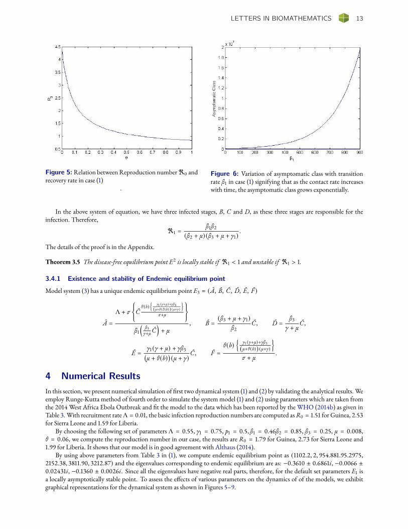
Figure 5: Relation betweenReproduction number<0 andrecovery rate in case (1)

.

Figure 6: Variation of asymptomatic class with transitionrate β1 in case (1) signifying that as the contact rate increaseswith time, the asymptomatic class grows exponentially.

In the above system of equation, we have three infected stages, B, C and D, as these three stages are responsible for theinfection. Therefore,

<1 =β1β2

(β2 + µ) (β3 + µ + γ1).

The details of the proof is in the Appendix.

Theorem 3.5 The disease-free equilibrium point E2 is locally stable if <1 < 1 and unstable if <1 > 1.

3.4.1 Existence and stability of Endemic equilibrium point

Model system (3) has a unique endemic equilibrium point E3 = (A, B, C , D, E, F )

A =

Λ + σ

{C

θ (b){

γ1 (γ+µ)+γβ3(µ+θ (D,b)) (µ+γ)

}σ+µ

}β1

(β3γ+µ C

)+ µ

, B =(β3 + µ + γ1)

β2C , D =

β3

γ + µC ,

E =γ1 (γ + µ) + γβ3(µ + θ(b)

)(µ + γ)

C , F =θ(b)

{γ1 (γ+µ)+γβ3(µ+θ (b)) (µ+γ)

}σ + µ

.

4 Numerical ResultsIn this section, we present numerical simulation of rst two dynamical system (1) and (2) by validating the analytical results. Weemploy Runge-Kutta method of fourth order to simulate the system model (1) and (2) using parameters which are taken fromthe 2014 West Africa Ebola Outbreak and t the model to the data which has been reported by the WHO (2014b) as given inTable 3. With recruitment rateΛ = 0.01, the basic infection reproduction numbers are computed asR0 = 1.51 for Guinea, 2.53for Sierra Leone and 1.59 for Liberia.

By choosing the following set of parameters Λ = 0.55, γ1 = 0.75, p1 = 0.5, β1 = 0.46β2 = 0.85, β3 = 0.25, µ = 0.008,θ = 0.06, we compute the reproduction number in our case, the results are R0 = 1.79 for Guinea, 2.73 for Sierra Leone and1.99 for Liberia. It shows that our model is in good agreement with Althaus (2014).

By using above parameters from Table 3 in (1), we compute endemic equilibrium point as (1102.2, 2, 954.881.95.2975,2152.38, 3811.90, 3212.87) and the eigenvalues corresponding to endemic equilibrium are as: −0.3610 ± 0.6861i, −0.0066 ±0.02431i, −0.1360 ± 0.0026i. Since all the eigenvalues have negative real parts, therefore, for the default set parameters E1 isa locally asymptotically stable point. To assess the eects of various parameters on the dynamics of of the models, we exhibitgraphical representations for the dynamical system as shown in Figures 5–9.


Figure 7: Change of<0, with parameters µ and β2 in (1). Figure 8: Variation of symptomatic class with time for dif-ferent values of γ1 = 0.25, 0.50, 0.75 in system (1).

Figure 9: Variation of population size with time for dierent values of δ = 0.5, 0.7, 0.9.

Figure 5 exhibits the relationship between reproduction number<0 and recovery rate θ in (1). When θ increases the num-ber of individuals getting treatment also increases and as a result the reproduction number decreases which is also biologicallyrelevant. Increasing θ suciently reduces the reproduction number below to 1.

Figure 6 displays the variation of asymptomatic class (1) with transition rate β1, which signies that as the contact rate in-creases with time, the asymptomatic class grows exponentially.

Figure 7depicts the relation among reproductionnumber (R0), disease-induceddeath rate (µ) and contact rate fromasymp-tomatic stage to symptomatic stage (β2) in (1). We observe that both the parameters namely the disease-induced death rate µand contact rate aects the reproduction number to large extent. As the values of both decrease, the reproduction number alsodecreases. It indicates that in order to eradicate the disease from environment, we need to control these parameters within asignicant level. However, the curve does not asymptotically become zero. It means diseases still prevails in the system.

Figure 8 demonstrates the eect of transition rate γ1 on symptomatic class in (1). It has been observed that as we increase thevalue of γ1 = 0.25, 0.50, 0.75, the symptomatic population decreases.

Since, in case of Ebola infection spread, dead bodies play a very crucial role, safe burial of death bodies is necessary to controlthis deadly virus. Figure 9 depicts the impact of removal of deaths from system which is described in model (2). It is note-worthy that as we increase the value of δ, the susceptible population rst decreases and then increases afterwards. The infectedcompartment as well decreases with increase in δ.


5 Discussion

This study aims to simulate the ebola epidemic with safe burial of its deaths taking into consideration of symptomatic andasymptomatic populationunder four dierent possible assumptions (four cases) of amathematicalmodel. In order to get insightof the dynamics of the transmission of ebola virus, model analysis is carried via computation of epidemic threshold quantities,reproduction number <0 (& <1 for the other cases) and stability of steady states. It is seen that the transitions rates fromsymptomatic (severed individuals) to individuals under treatment have negative eect on reproduction number as 𝜕<0

𝜕γ1< 0 and

𝜕<0𝜕γ < 0, which indicates that earlier the symptomatic and severed infected individuals enter treatment class, the faster<0 canbe reduced. Epidemiologically, it infers that early treatment is critical to controlling the disease when completely safe burial isnot possible.

Further, we compare our results of reproduction number (8)with the results ofAlthaus (2014). In 2014, Althaus developeda predictive SEIRmathematicalmodel onEbola virus andtted themodel to the datawhich has been reported fromWHO[datais available seeWHO (2014b)] of three African countries namely Guinea, Sierra Leone and Liberia. Basic reproduction numberinAlthaus (2014) is estimated asR0 = 1.51 forGuinea, 2.53 for Sierra Leone and 1.59 for Liberia. We compute the reproductionnumber for ourmodel with our estimated parameters and found higher but reasonable (in good agreement with Althaus (2014)values ofR0 = 1.79 for Guinea, 2.73 for Sierra Leone and 1.99 for Liberia. This increase in higher estimate can be attributed toner level of characterisation of our infection stages as seen in epidemiology of a patient.

Moreover, it has been observed that the parameters such as disease-induced death rate and contact rate from asymptomaticstage to symptomatic stage aecting the Reproduction number to larger extent as compared to the demographic and disease-progression related parameters. Our model is based on system of nonlinear ordinary dierential equations (ODEs) which isanalyzed using bifurcation analysis and provides some useful information on the spread of Ebola virus under the assumption ofsafe and unsafe burial practices of its deaths. The safe burial of those who have died of Ebola is acknowledged as an importantintervention for controlling epidemics. In earlier work of Xia et al. (2015) and Chowell et al. (2015), authors have consideredburial aspect but they have not emphatically considered safe burial as safety intervention neither they have incorporated vac-cination or resource limitation in their model, we have considered safe burial as one of the major controlling strategies as wellas vaccination intervention. Our works is dierent from previous work, as we divide the infection stages into three sub-classesnamely: asymptomatic, symptomatic and severed infected with safe burial which is in line with actual situation in case of ebolaepidemic. We consider here four cases: (i) transmission of Ebola with safe burial (case 1), (ii) without safe burial and possibilityof direct severed infection in some cases (case 2), (iii) role of availability of vaccination intervention in the population (case 3),and (iv) transmission dynamics of Ebola spread when treatment intervention is limited by resources. Our results have identieddisease persistence threshold quantity,R0, and endemic levels in each of the four cases. We have classied four distinct scenarios(corresponding to four cases) in terms of ecacy of various interventions (safe burial, unsafe burial, vaccination and treatmenteciency).

There has been many direction in which this work can further be extended by examining the inuence of human culturaland movement behaviours on ebola virus transmission. However, it may be dicult to nd appropriate data to parameterizesuchmodels. Aswith other diseases, appropriate empirical studies are in need to comprehensively understanddynamics of Ebolawith varied practices and interventions in dierent parts of the world, potential driven by social determinants of health (such ascultures).

6 Conclusion

In this article, a deterministicmathematicalmodel and its four cases for understanding the impact of treatment, vaccination, andburial practices related interventions on transmission dynamic of Ebola virus with limited and unlimited healthcare resourcesare analysed. The model cases has two equilibrium points namely disease-free and endemic equilibrium. It has shown that thedisease-free equilibrium is a locally asymptotically stable when reproduction number is less than unity and endemic equilibriumpoint is asymptotically stable when reproduction number is greater than unity. Sensitivity analysis is carried out on the modeloutputs to assess the eects of timely treatment and safe burial dead bodies on control of Ebola. We conclude that re-emergenceof infection after eective treatment is a valuable aspect which deserves more attention and intervention strategies to reduce theEbola virus eect on human population. Further, the treatment ecacy used in treatment of Ebola virus plays a signicant rolein reduction of dynamics of the virus. Our study has not considered the rates as variable which is more realistic. The futureextension of our investigation will be the variables as function of time. We will also incorporate demographic and geographiceects on the dynamics of the Ebola virus.


Acknowledgments

The authors are thankful to the anonymous referees and Prof. Anuj Mubayi for their valuable comments & suggestions thathelp to improve the quality of this manuscript.

Conflict of Interest

The work has no potential conict of interest.

ReferencesAbdelrazec, A., J. Bélair, C. Shan, and H. Zhu (2016). Modeling the spread and control of dengue with limited public healthresources. Mathematical biosciences 271, 136–145. 2, 3

Agusto, F. (2017). Mathematical model of ebola transmission dynamics with relapse and reinfection. Mathematical bio-sciences 283, 48–59. 2

Ahmad, M., M. A. Khan, S. Ullah, M. Farooq, and T. Gul (2019). Modeling the transmission dynamics of tuberculosis inkhyber pakhtunkhwa pakistan. Advances inMechanical Engineering 11(6), 1687814019854835. 2

Althaus, C. L. (2014). Estimating the reproduction number of ebola virus (ebov) during the 2014 outbreak in west africa. PLoScurrents 6. 2, 13, 15

Area, I., H. Batar, J. Losada, J. J. Nieto, W. Shammakh, and Á. Torres (2015). On a fractional order ebola epidemic model.Advances in Dierence Equations 2015(1), 278. 2

Carr, J. (2012). Applications of centre manifold theory, Volume 35. Springer Science & Business Media. 6, 9

CDC (2014). Centers for disease control and prevention. ebola outbreak in west africa-case counts november 2014. Centres forDisease Control and Prevention 0. 1

Chowell, D., C.Castillo-Chavez, S. Krishna, X.Qiu, andK. S. Anderson (2015). Modelling the eect of early detection of ebola.The Lancet Infectious Diseases 15(2), 148–149. 2, 6, 15

Chowell, G., N.W.Hengartner, C. Castillo-Chavez, P.W. Fenimore, and J.M.Hyman (2004). The basic reproductive numberof ebola and the eects of public health measures: the cases of congo and uganda. Journal of theoretical biology 229(1), 119–126. 2

Chowell, G. and H. Nishiura (2014). Transmission dynamics and control of ebola virus disease (evd): a review. BMCmedicine 12(1), 196. 2

Dhillon, R. S., D. Srikrishna, R. F. Garry, and G. Chowell (2015). Ebola control: rapid diagnostic testing. The Lancet InfectiousDiseases 15(2), 147–148. 2

Diekmann, O., J. A. P. Heesterbeek, and J. A. Metz (1990). On the denition and the computation of the basic reproductionratio r 0 in models for infectious diseases in heterogeneous populations. Journal of mathematical biology 28(4), 365–382. 2,6

Du Toit, A. (2014). Ebola virus in west africa. Nature ReviewsMicrobiology 12(5), 312–312. 1

ELRhoubari, Z., H. Besbassi, K.Hattaf, andN. Yous (2018). Mathematical modeling of ebola virus disease in bat population.Discrete Dynamics in Nature and Society 2018. 2

Feldmann, H. and T. W. Geisbert (2011). Ebola haemorrhagic fever. The Lancet 377 (9768), 849–862. 1

Feldmann, H., S. Jones, H.-D. Klenk, and H.-J. Schnittler (2003). Ebola virus: from discovery to vaccine. Nature ReviewsImmunology 3(8), 677–685. 1

Feng, Z., C. Castillo-Chavez, and A. F. Capurro (2000). A model for tuberculosis with exogenous reinfection. Theoreticalpopulation biology 57 (3), 235–247. 2

Feng, Z. and J. X. Velasco-Hernández (1997). Competitive exclusion in a vector-host model for the dengue fever. Journal ofmathematical biology 35(5), 523–544. 2


Grigorieva, E. and E. Khailov (2014). Optimal vaccination, treatment, and preventive campaigns in regard to the sir epidemicmodel. MathematicalModelling of Natural Phenomena 9(4), 105–121. 2

Hewlett, B. S. andR. P. Amola (2003). Cultural contexts of ebola in northern uganda. Emerging infectious diseases 9(10), 1242.3

Huo, H.-F. and L.-X. Feng (2013). Global stability for an hiv/aids epidemic model with dierent latent stages and treatment.AppliedMathematicalModelling 37 (3), 1480–1489. 2

Jiang, S., K. Wang, C. Li, G. Hong, X. Zhang, M. Shan, H. Li, and J. Wang (2017). Mathematical models for devising theoptimal ebola virus disease eradication. Journal of translational medicine 15(1), 124. 2

Jones, A. K. (2017). Green computing: new challenges and opportunities. In Proceedings of the on Great Lakes Symposium onVLSI 2017, pp. 3–3. 2

Kabli, K., S. El Moujaddid, K. Niri, and A. Tridane (2018). Cooperative system analysis of the ebola virus epidemic model.Infectious DiseaseModelling 3, 145–159. 2

Khan, M., A. Khan, A. Elsonbaty, and A. Elsadany (2019). Modeling and simulation results of a fractional dengue model. TheEuropean Physical Journal Plus 134(8), 379. 2

Korobeinikov, A. and G. C. Wake (2002). Lyapunov functions and global stability for sir, sirs, and sis epidemiological models.AppliedMathematics Letters 15(8), 955–960. 9

Kortepeter, M. G., D. G. Bausch, andM. Bray (2011). Basic clinical and laboratory features of loviral hemorrhagic fever. TheJournal of infectious diseases 204(suppl_3), S810–S816. 1

LaSalle, J. P. (1976). The stability of dynamical systems, Volume 25. Siam. 2, 10

Legrand, J., R. F. Grais, P.-Y. Boelle, A.-J. Valleron, and A. Flahault (2007). Understanding the dynamics of ebola epidemics.Epidemiology & Infection 135(4), 610–621. 2

Madubueze, C. E., A. R. Kimbir, and T. Aboiyar (2018). Global stability of ebola virus disease model with contact tracing andquarantine. Applications & AppliedMathematics 13(1). 2

Martyushev, A., S. Nakaoka, K. Sato, T. Noda, and S. Iwami (2016). Modelling ebola virus dynamics: Implications for therapy.Antiviral research 135, 62–73. 2

Mubayi, A., C. K. Zaleta, M. Martcheva, and C. Castillo-Chávez (2010). A cost-based comparison of quarantine strategies fornew emerging diseases. Mathematical Biosciences & Engineering 7 (3), 687. 2

Nielsen, C. F., S. Kidd, A. R. Sillah, E. Davis, J. Mermin, and P. H. Kilmarx (2015). Improving burial practices and ceme-tery management during an ebola virus disease epidemic—sierra leone, 2014. MMWR. Morbidity and mortality weeklyreport 64(1), 20. 2

Peters, C. and J. Peters (1999). An introduction to ebola: the virus and the disease. The Journal of Infectious Dis-eases 179(Supplement_1), ix–xvi. 3

Rachah, A. and D. F. Torres (2015). Mathematical modelling, simulation, and optimal control of the 2014 ebola outbreak inwest africa. Discrete Dynamics in Nature and Society 2015. 2

Rachah, A. and D. F. Torres (2016). Dynamics and optimal control of ebola transmission. Mathematics in Computer Sci-ence 10(3), 331–342. 2

Rachah, A. and D. F. Torres (2017). Predicting and controlling the ebola infection. Mathematical Methods in the AppliedSciences 40(17), 6155–6164. 2

Rathore, K., R. Keshari, A. Rathore, and D. Chauhan (2014). A review on ebola virus disease. PharmaTutor 2(10), 17–22. 1

Singh, R., S. Ali, M. Jain, and A. A. Raina (2019). Mathematical model for malaria with mosquito-dependent coecient forhuman population with exposed class. Journal of the National Science Foundation of Sri Lanka 47 (2). 2


Singh, R., M. Jain, and S. Ali (2016). Mathematical analysis of transmission dynamics of tuberculosis with recurrence based ontreatment. In 2016 International Conference on Electrical, Electronics, and Optimization Techniques (ICEEOT), pp. 3995–4000. IEEE. 2

Singh, R., P. Preeti, and A. A. Raina (2018). Markovian epidemic queueing model with exposed, infection and vaccinationbased on treatment. World Scientific News 106, 141–150. 2

Singh, R., G. Sharma, andM. Jain (2010). Mathematical modeling of blood ow in a stenosed artery under mhd eect throughporous medium. International Journal of Engineering 23(3), 243–252. 2

Singh, R. and N. Sharma (2018). Computational modeling and analysis of transmission dynamics of zika virus based on treat-ment. Int.J Sci.Res.Compt.Sc, Engg & IT 4, 111–116. 2

Summers, D. J., R. W. Acosta, and A. M. Acosta (2015). Zika virus in an american recreational traveler. Journal of travelmedicine 22(5), 338–340. 1

Ullah, S., M. A. Khan, M. Farooq, and T. Gul (2019). Modeling and analysis of tuberculosis (tb) in khyber pakhtunkhwa,pakistan. Mathematics and Computers in Simulation 165, 181–199. 2

Ullah, S., M. A. Khan, and J. Gómez-Aguilar (2019). Mathematical formulation of hepatitis b virus with optimal controlanalysis. Optimal Control Applications andMethods 40(3), 529–544. 2

van denDriessche, P. (2017). Reproduction numbers of infectious disease models. Infectious DiseaseModelling 2(3), 288–303.8

van den Driessche, P. and J. Watmough (2002). Reproduction numbers and sub-threshold endemic equilibria for compart-mental models of disease transmission. Mathematical biosciences 180(1-2), 29–48. 7

Wang, X.-S. and L. Zhong (2015). Ebola outbreak in west africa: real-time estimation and multiple-wave prediction. arXivpreprint arXiv:1503.06908. 2

Wasim, S., M. Khan, A. Shah, S. Ullah, and J. Gómez-Aguilar (2019). A dynamical model of asymptomatic carrier zika viruswith optimal control strategies. Nonlinear Analysis: RealWorld Applications 50, 144–170. 2

Weitz, J. S. and J. Dusho (2015). Modeling post-death transmission of ebola: challenges for inference and opportunities forcontrol. Scientific reports 5, 8751. 2

WHO (2014a). World health organization report, ebola virus disease fact sheet. World Health Organization 0(103). 1

WHO (2014b). World health organization(who)who statement on the meeting of the international health regulations emer-gency committee regarding the 2014 ebola outbreak in west africa geneva. World Health Organization 0. 1, 13, 15

Xia, Z.-Q., S.-F. Wang, S.-L. Li, L.-Y. Huang, W.-Y. Zhang, G.-Q. Sun, Z.-T. Gai, and Z. Jin (2015). Modeling the transmissiondynamics of ebola virus disease in liberia. Scientific reports 5, 13857. 2, 15

Yusuf, T. T. and F. Benyah (2012). Optimal strategy for controlling the spread of hiv/aids disease: a case study of south africa.Journal of biological dynamics 6(2), 475–494. 2

Zhu, J.-M., L. Wang, and J.-B. Liu (2016). Eradication of ebola based on dynamic programming. Computational and mathe-matical methods in medicine 2016. 2

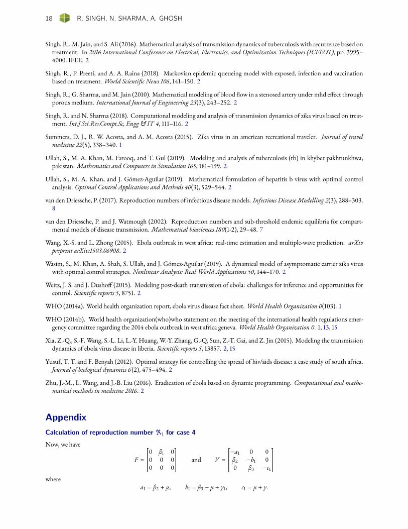
AppendixCalculation of reproduction number <1 for case 4

Now, we have

F =0 β1 00 0 00 0 0

and V =−a1 0 0β2 −b1 00 β3 −c1

where

a1 = β2 + µ, b1 = β3 + µ + γ1, c1 = µ + γ.


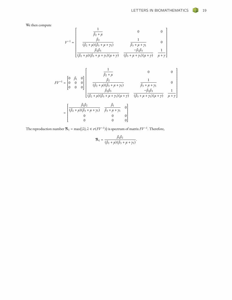
We then compute

V−1 =

1β2 + µ

0 0

β2

(β2 + µ) (β3 + µ + γ1)1

β3 + µ + γ10

β2β3

(β2 + µ) (β3 + µ + γ1) (µ + γ)−β2β3

(β3 + µ + γ1) (µ + γ)1

µ + γ

FV−1 =0 β1 00 0 00 0 0

1β2 + µ

0 0

β2

(β2 + µ) (β3 + µ + γ1)1

β3 + µ + γ10

β2β3

(β2 + µ) (β3 + µ + γ1) (µ + γ)−β2β3

(β3 + µ + γ1) (µ + γ)1

µ + γ

=

β1β2

(β2 + µ) (β3 + µ + γ1)β1

β3 + µ + γ10

0 0 00 0 0

The reproduction number<1 = max

(|λ|; λ ∈ σ (FV−1)

)is spectrum of matrix FV−1. Therefore,

<1 =β1β2

(β2 + µ) (β3 + µ + γ1).

An Application to Ebola Type Infectious Disease - Letters in ...

Documents

Transcript of An Application to Ebola Type Infectious Disease - Letters in ...