An analytical model of the effects of catchment

elevation on the flood frequency distribution

P. Allamano,1 P. Claps,1 and F. Laio1

Received 14 November 2007; revised 26 September 2008; accepted 15 October 2008; published 3 January 2009.

[1] The effect of temperature on the flood frequency distribution in mountainous basins isexamined through a minimalist analytical model. The conceptual hypothesis on whichthe model is grounded is the existence of a subtractive mechanism that reduces thebasin-contributing area in flood formation to the fraction of basin laying belowthe freezing elevation at the time of occurrence of each precipitation event. This fractiondepends on the watershed hypsometric curve and on the seasonal evolution oftemperatures. Under this hypothesis, the probability distribution of the annual maximumdischarge is analytically derived, based on simple assumptions on the stochastic process ofprecipitation. The shape and the moments of this distribution explicitly relate tobasin hypsometry and to the seasonality of temperatures. Qualitative results show that thesimple causative mechanisms can explain the attenuation of flood quantiles inhigh-elevation basins. Model application to 57 watersheds in the Northwestern ItalianAlps effectively demonstrates the role of the hypsography in explaining the spatialvariability of the mean of the flood distribution.

Citation: Allamano, P., P. Claps, and F. Laio (2009), An analytical model of the effects of catchment elevation on the flood

frequency distribution, Water Resour. Res., 45, W01402, doi:10.1029/2007WR006658.

1. Introduction

[2] The study of the flood formation processes in moun-tainous basins has traditionally received less attention thanin temperate regions. The reason is probably related to adistinct perception of a limited flood risk in the coldenvironments because of the mitigating effect exerted bythe snowfall that does not contribute immediately to runoff.Although this perception is easy to prove using hydrologicmodeling, few attempts have been made [see e.g., Loukas,2002] of traducing the principle of partially contributingmountain basin into a flood frequency model. Besides therelevance of this principle for a better understanding of theflood processes, the topic assumes practical importancewhen affording a regional flood frequency analysis in amountainous region. In high-elevation basins, in fact, thedifficulty of gathering observations of precipitation andrunoff makes it possibly more urgent than for the temperatebasins the need of connecting flood frequency distributionsto physically-consistent flood producing mechanisms.[3] The ensemble of flood-producing mechanisms, in-

cluding rainfall, snowmelt, and rain-on-snow in spring, rainon frozen ground in winter, and thundershowers in summer[Loukas et al., 2000; Bacchi and Ranzi, 2003; Merz andBloschl, 2003; Singh et al., 2005] might suggest the use ofdetailed hydrological models to produce the flood frequencycurve, for example, by means of Monte-Carlo simulations[e.g., Littlewood, 2002; Rahman et al., 2002; Loukas,2002]. Such an approach however always requires some

kind of calibration of the hydrological model parameters(assisted by consistent data availability) that prevents theuse of these methods for flood risk assessment in ungaugedbasins.[4] An alternative statistically sound approach considers

that the different flood formation mechanisms coexisting inmountainous basins would produce flood frequency curvesrepresentable by mixed distributions [e.g., Waylen and Woo,1982; Rossi et al., 1984; Buishand and Demare, 1990; Alilaand Mtiraoui, 2002; Sivapalan et al., 2005]. This purelystatistical approach still does not prove to be effective inregional analysis, because the flood frequency distributionbecomes heavily parameterized and, so far, the parametershave not been connected to physical basin characteristics.[5] A more promising avenue of research, at least for the

understanding of the dominant processes in the floodformation, is one which introduces some physical knowl-edge in the construction of the flood frequency curve,usually called the derived distribution approach [see e.g.,Eagleson, 1972; Gottschalk and Weingartner, 1998;Iacobellis and Fiorentino, 2000; De Michele and Salvadori,2002]. This is the approach adopted in this work, where theflood producing mechanisms and a stochastic forcing aretransposed into a flood frequency curve in parametric andanalytical form. This kind of approach stems from theconviction that, in complex contexts, models with a simpleand controllable framework can provide a valuable com-promise between real processes and data. In this respect, thephilosophy of this work is akin to that of Eagleson [1978],Milly [1994a, 1994b], Rodriguez Iturbe et al. [2001],Woods[2003], Perona et al. [2007] among others.[6] Simplifying, yet realistic, assumptions are made to

keep the analytical tractability of the proposed model(sections 2 and 3). As in the cited examples, the devised

1Dipartimento di Idraulica, Trasporti ed Infrastrutture Civili, Politecnicodi Torino, Torino, Italy.

Copyright 2009 by the American Geophysical Union.0043-1397/09/2007WR006658$09.00

W01402

WATER RESOURCES RESEARCH, VOL. 45, W01402, doi:10.1029/2007WR006658, 2009ClickHere

for

FullArticle

1 of 12

theoretical mechanistic model find its justification in theformulation of an analytical representation of the interactionof the forcing processes with the system characteristics,allowing one to easily perform a full sensitivity analysis ofmodel results (section 4). To answer the question if themodel structure is too simple to represent the actual out-come of the complex combination of causative processes,we rely on the possibility of validating the probabilisticmodel. In this case, in fact, we consider also real data tovalidate the overall behavior of the model and verify themodel representativeness on a large geographical scale. Thisis done by comparing the observed variability of the meanannual flood with the behavior resulting from the modelapplication (section 5). A discussion on the results and onthe open problems to be addressed in future research closesthe paper.

2. Model Structure

[7] The basic conceptual hypothesis on which the modelis grounded consists in the existence of an elevation-drivensubtractive mechanism that reduces the active portion of thewatershed in flood formation. This mechanism is identifiedwith the concept of contributing area (Ac), defined as theportion of the basin area (A) that is immediately involved inrunoff formation. Runoff forming areas have previously beenassociated mainly with soil water processes (for example,infiltration-excess runoff, saturation-excess runoff, subsur-face streamflow) [Eagleson, 1972;Wood and Hebson, 1986;Bloschl and Sivapalan, 1997; Ambroise, 2004]. Here we takea broader view and consider runoff-forming areas to be thoseareas where rain falls as liquid rather than solid water. Inmountainous basins, in fact, for a given flood event, thecontributing area Ac depends on the elevation at whichtransition from solid to liquid precipitation takes place,hereafter identified, for simplicity, as the zero-degreesisothermal, ZT(t), or freezing elevation. According to thisdefinition each precipitation event produces rainfall overthe fraction Ac/A of the basin below the freezing elevationand snowfall in the upper part of the basin, the latter notcontributing directly to discharge.[8] This study aims at quantifying the role of this parti-

tioning on flood discharge, by considering the direct runoff(q) as the result of a mechanism that can be formulated asfollows:

q ¼ C � fc tð Þ � hþ SM tð Þ ð1Þ

where C is the peak runoff coefficient, fc(t) = Ac/A is thecontributing area fraction, with 0 � fc(t) � 1, h is the rainfalldepth and t is the Julian date. We model rainfall accordingto the very common Poisson representation of storm arrivalsin time with rate l, each storm having a depth h modeled asan exponentially distributed random variable with mean a.A deterministic component SM(t) is added to this rainfall-runoff component to account for the snow meltingcontribution during the warm season. Possible presence ofseasonal variation in the rate l and average rainfall intensitya could be accounted for by using a non-homogeneousmarked Poisson process for rainfall.[9] Two different interpretations of equation (1) are

possible: h can be supposed to represent the total precipi-

tation volume in a given storm, in which case a and h areexpressed in mm and q represents the runoff volume perunit area, again expressed in mm. Alternatively, one cansuppose to determine, for each storm event, the maximumprecipitation intensity averaged over a duration d, and callthis intensity h. For example, the duration d can be takenequal to 1 day, in which case q is a daily discharge per unitarea, with the same units as a (for example, mm/d). Theduration can also be supposed to vary from basin to basinand to be equal to some critical precipitation duration, forinstance the one that maximizes the instantaneous peakdischarge. When h is a precipitation intensity averaged overa critical duration, equation (1) becomes analogous to thestandard rational formula, and q has the form of aninstantaneous discharge per unit area, again with the sameunits as a (for example, mm/h or mm/d). Either of theseinterpretations can be adopted without affecting the generalresults of the model: in fact, the partitioning into liquid andsolid precipitation is reasonably independent of the specificduration considered. In the following we will therefore referto q as a generic discharge value, except than in the finalapplication where we will use instantaneous discharge datato test the model.[10] Under these premises, the distribution of the dis-

charge q conditioned on the Julian date t, PQjT(qjt), can befound as a derived distribution. Starting from the cumulativedistribution of the precipitation events, PH(h) = 1� exp(�h/a),and using equation (1) one finds

PQjT qjtð Þ ¼ 1� exp � q� SM tð ÞCa � fc tð Þ

� �; ð2Þ

in which SM(t) plays the role of the position parameter, andthe product Cafc(t) that of the scale parameter.[11] According to the Bayes theorem, the marginal cu-

mulative distribution of discharge PQ(q) can then beexpressed as

PQ qð Þ ¼Zt

PQjT qjtð Þ � pT tð Þ � dt ð3Þ

where PQjT(qjt) is the conditional probability in equation (2)and pT(t) is the probability density function of the date ofoccurrence of the events. Supposing that the precipitationevents form an homogeneous Poisson sequence in time,one has pT(t) = 1/365, i.e. the days of occurrence havea uniform probability density function [e.g., Ross, 1996,p. 66].[12] Another consequence of the Poisson hypothesis is

that the probability distribution of the discharge annualextremes PQAM

(q) assumes the form [e.g., Coles, 2001, p.131]

PQAMqð Þ ¼ exp �l � 1� PQ qð Þ

� �� �ð4Þ

where QAM are the annual maxima of discharge and PQ(q)is the marginal cumulative distribution of discharge inequation (3). For a basin having very low elevations, wherethe contributing area fraction is constant and equal to 1 allover the year (i.e. the whole basin contributes to runoff)and the snowmelt contribution is null, the expression

2 of 12

W01402 ALLAMANO ET AL.: EFFECTS OF ELEVATION ON FLOOD FREQUENCY DISTRIBUTION W01402

equation (4) reduces to the well-known form of the Gumbeldistribution

PQAMqð Þ ¼ exp �l � exp � q

Ca

� �� �ð5Þ

that we will sometimes refer to as ‘‘undisturbed’’ floodfrequency distribution. The difference between the twocurves equations (4) and (5) is a measure of the relevanceof snow processes in shaping the flood frequencydistribution in mountainous areas.

3. Model Specification

[13] To specify the analytical framework behindequation (3), the mathematical representations for fc(t) andSM(t) are required. These representations should be necessar-ily simple to keep the derived distribution in analytical form.

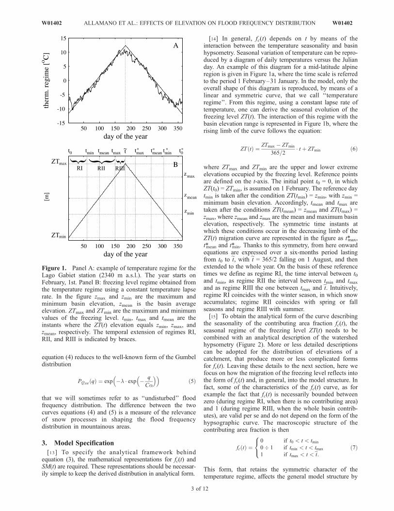
[14] In general, fc(t) depends on t by means of theinteraction between the temperature seasonality and basinhypsometry. Seasonal variation of temperature can be repro-duced by a diagram of daily temperatures versus the Julianday. An example of this diagram for a mid-latitude alpineregion is given in Figure 1a, where the time scale is referredto the period 1 February–31 January. In the model, only theoverall shape of this diagram is reproduced, by means of alinear and symmetric curve, that we call ‘‘temperatureregime’’. From this regime, using a constant lapse rate oftemperature, one can derive the seasonal evolution of thefreezing level ZT(t). The interaction of this regime with thebasin elevation range is represented in Figure 1b, where therising limb of the curve follows the equation:

ZT tð Þ ¼ ZTmax � ZTmin

365=2� t þ ZTmin ð6Þ

where ZTmax and ZTmin are the upper and lower extremeelevations occupied by the freezing level. Reference pointsare defined on the t-axis. The initial point t0 = 0, in whichZT(t0) = ZTmin, is assumed on 1 February. The reference daytmin is taken after the condition ZT(tmin) = zmin, with zmin =minimum basin elevation. Accordingly, tmean and tmax aretaken after the conditions ZT(tmean) = zmean and ZT(tmax) =zmax, where zmean and zmax are the mean and maximum basinelevation, respectively. The symmetric time instants atwhich these conditions occur in the decreasing limb of theZT(t) migration curve are represented in the figure as t*max,t*mean and t*min. Thanks to this symmetry, from here onwardequations are expressed over a six-months period lastingfrom t0 to et, with et = 365/2 falling on 1 August, and thenextended to the whole year. On the basis of these referencetimes we define as regime RI, the time interval between t0and tmin, as regime RII the interval between tmin and tmax

and as regime RIII the one between tmax and et. Intuitively,regime RI coincides with the winter season, in which snowaccumulates; regime RII coincides with spring or fallseasons and regime RIII with summer.[15] To obtain the analytical form of the curve describing

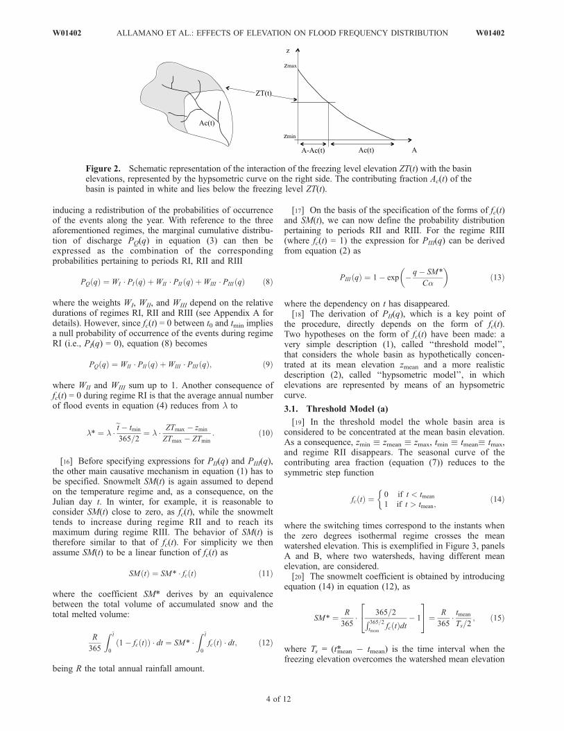
the seasonality of the contributing area fraction fc(t), theseasonal regime of the freezing level ZT(t) needs to becombined with an analytical description of the watershedhypsometry (Figure 2). More or less detailed descriptionscan be adopted for the distribution of elevations of acatchment, that produce more or less complicated formsfor fc(t). Leaving these details to the next section, here wefocus on how the migration of the freezing level reflects intothe form of fc(t) and, in general, into the model structure. Infact, some of the characteristics of the fc(t) curve, as forexample the fact that fc(t) is necessarily bounded betweenzero (during regime RI, when there is no contributing area)and 1 (during regime RIII, when the whole basin contrib-utes), are valid per se and do not depend on the form of thehypsographic curve. The macroscopic structure of thecontributing area fraction is then

fc tð Þ ¼0 if t0 < t < tmin

0 1 if tmin < t < tmax

1 if tmax < t <et:8<: ð7Þ

This form, that retains the symmetric character of thetemperature regime, affects the general model structure by

Figure 1. Panel A: example of temperature regime for theLago Gabiet station (2340 m a.s.l.). The year starts onFebruary, 1st. Panel B: freezing level regime obtained fromthe temperature regime using a constant temperature lapserate. In the figure zmax and zmin are the maximum andminimum basin elevation, zmean is the basin averageelevation. ZTmax and ZTmin are the maximum and minimumvalues of the freezing level. tmin, tmax and tmean are theinstants where the ZT(t) elevation equals zmin, zmax, andzmean, respectively. The temporal extension of regimes RI,RII, and RIII is indicated by braces.

W01402 ALLAMANO ET AL.: EFFECTS OF ELEVATION ON FLOOD FREQUENCY DISTRIBUTION

3 of 12

W01402

inducing a redistribution of the probabilities of occurrenceof the events along the year. With reference to the threeaforementioned regimes, the marginal cumulative distribu-tion of discharge PQ(q) in equation (3) can then beexpressed as the combination of the correspondingprobabilities pertaining to periods RI, RII and RIII

PQ qð Þ ¼ WI � PI qð Þ þWII � PII qð Þ þWIII � PIII qð Þ ð8Þ

where the weights WI, WII, and WIII depend on the relativedurations of regimes RI, RII and RIII (see Appendix A fordetails). However, since fc(t) = 0 between t0 and tmin impliesa null probability of occurrence of the events during regimeRI (i.e., PI(q) = 0), equation (8) becomes

PQ qð Þ ¼ WII � PII qð Þ þWIII � PIII qð Þ; ð9Þ

where WII and WIII sum up to 1. Another consequence offc(t) = 0 during regime RI is that the average annual numberof flood events in equation (4) reduces from l to

l* ¼ l �et � tmin

365=2¼ l � ZTmax � zmin

ZTmax � ZTmin

: ð10Þ

[16] Before specifying expressions for PII(q) and PIII(q),the other main causative mechanism in equation (1) has tobe specified. Snowmelt SM(t) is again assumed to dependon the temperature regime and, as a consequence, on theJulian day t. In winter, for example, it is reasonable toconsider SM(t) close to zero, as fc(t), while the snowmelttends to increase during regime RII and to reach itsmaximum during regime RIII. The behavior of SM(t) istherefore similar to that of fc(t). For simplicity we thenassume SM(t) to be a linear function of fc(t) as

SM tð Þ ¼ SM* � fc tð Þ ð11Þ

where the coefficient SM* derives by an equivalencebetween the total volume of accumulated snow and thetotal melted volume:

R

365

Z ~t

0

1� fc tð Þð Þ � dt ¼ SM* �Z ~t

0

fc tð Þ � dt; ð12Þ

being R the total annual rainfall amount.

[17] On the basis of the specification of the forms of fc(t)and SM(t), we can now define the probability distributionpertaining to periods RII and RIII. For the regime RIII(where fc(t) = 1) the expression for PIII(q) can be derivedfrom equation (2) as

PIII qð Þ ¼ 1� exp � q� SM*

Ca

� �ð13Þ

where the dependency on t has disappeared.[18] The derivation of PII(q), which is a key point of

the procedure, directly depends on the form of fc(t).Two hypotheses on the form of fc(t) have been made: avery simple description (1), called ‘‘threshold model’’,that considers the whole basin as hypothetically concen-trated at its mean elevation zmean and a more realisticdescription (2), called ‘‘hypsometric model’’, in whichelevations are represented by means of an hypsometriccurve.

3.1. Threshold Model (a)

[19] In the threshold model the whole basin area isconsidered to be concentrated at the mean basin elevation.As a consequence, zmin zmean zmax, tmin tmean tmax,and regime RII disappears. The seasonal curve of thecontributing area fraction (equation (7)) reduces to thesymmetric step function

fc tð Þ ¼ 0 if t < tmean

1 if t > tmean;

�ð14Þ

where the switching times correspond to the instants whenthe zero degrees isothermal regime crosses the meanwatershed elevation. This is exemplified in Figure 3, panelsA and B, where two watersheds, having different meanelevation, are considered.[20] The snowmelt coefficient is obtained by introducing

equation (14) in equation (12), as

SM* ¼ R

365� 365=2R 365=2

tmeanfc tð Þdt

� 1

24 35 ¼ R

365� tmean

Ts=2; ð15Þ

where Ts = (t*mean � tmean) is the time interval when thefreezing elevation overcomes the watershed mean elevation

Figure 2. Schematic representation of the interaction of the freezing level elevation ZT(t) with the basinelevations, represented by the hypsometric curve on the right side. The contributing fraction Ac(t) of thebasin is painted in white and lies below the freezing level ZT(t).

4 of 12

W01402 ALLAMANO ET AL.: EFFECTS OF ELEVATION ON FLOOD FREQUENCY DISTRIBUTION W01402

(regime RIII) and snowmelt occurs. Equation (11) reducesto

SM tð Þ ¼ 0 if t 2 TsSM* if t =2 Ts

�ð16Þ

where snowmelt is produced at a constant rate SM* duringTs, while snow is considered to accumulate during theremaining period, that lasts [365 � Ts] days. An increase inthe mean basin elevation induces a reduction of the intervalTs and an increase in the accumulated volume, being SM* inequation (15) inversely proportional to Ts.[21] Given the above assumptions,WIII = 1 in equation (9)

and PQ(q) assumes the form outlined in equation (13). Theflood distribution is found by introducing l* and PQ(q) intoequation (4), obtaining

PQAMqð Þ ¼ exp �l* � exp � q� SM*

Ca

� �� �: ð17Þ

This curve is plotted as a solid black line in Figure 4 for twobasins having different mean elevations. In the samediagram the grey thick line represents the undisturbed floodfrequency distribution (equation (5)). Further comments onthe shapes of these functions and an explanation for thedashed black curve are given in the following section.

3.2. Hypsometric Model (b)

[22] A more realistic representation of the distribution ofelevations within a watershed is given by the hypsometric

curve, which is the cumulative frequency curve of eleva-tions of all the points in a basin. A mathematical approx-imation of the empirical hypsometric curve is used byadopting the one-parameter function [Strahler, 1952]:

z� zmin

zmax � zmin

¼ fc tð Þ1þ z � 1� fc tð Þð Þ ; ð18Þ

where z (with zmin < z < zmax) is the elevation that partitionsthe watershed into a contributing and non-contributing areaand z is a parameter controlling the flexure of the curve, thatassumes only values greater than �1. Setting the freezingelevation ZT(t) for z in equation (18), one finds a piecewiseexpression for the contributing area fraction

fc tð Þ ¼

0 t0 < t < tmin

1þ zð Þ ZT tð Þ � zminð Þz ZT tð Þ � zminð Þ þ zmax � zmin

tmin < t < tmax

1 tmax < t <et:

8>>><>>>: ð19Þ

In this case the no-flood interval is [t0 � tmin], whichproduces l* according to equation (10).[23] Given the above assumptions, the hypsometric mod-

el further specifies into different sub-cases, that refer towatersheds interacting with the ZT(t) curve in different ways(see Table 1): a case (b1) which refers to a watershed havingzmin > ZTmin and zmax < ZTmax (called ‘‘bounded water-shed’’), where all regimes RI, RII, and RIII actually exist; acase (b2) (called ‘‘high-elevationwatershed’’) which presents

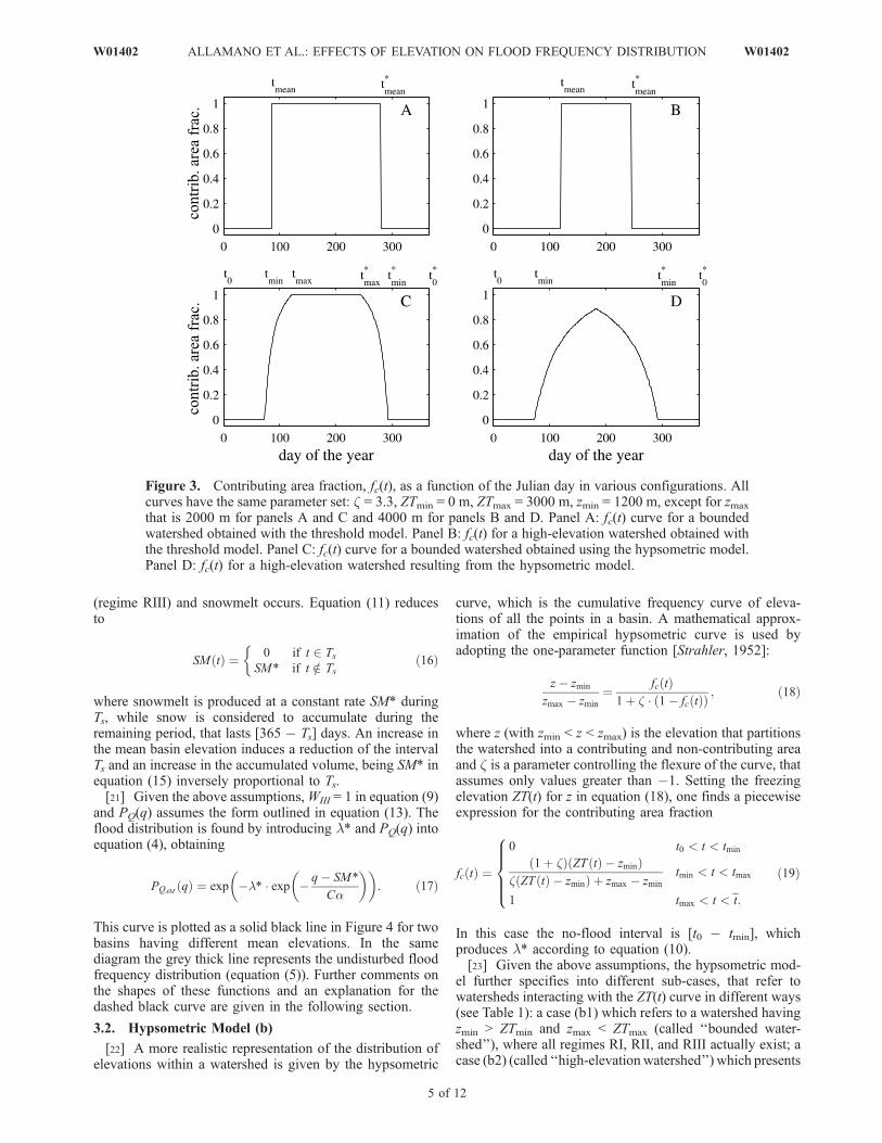
Figure 3. Contributing area fraction, fc(t), as a function of the Julian day in various configurations. Allcurves have the same parameter set: z = 3.3, ZTmin = 0 m, ZTmax = 3000 m, zmin = 1200 m, except for zmax

that is 2000 m for panels A and C and 4000 m for panels B and D. Panel A: fc(t) curve for a boundedwatershed obtained with the threshold model. Panel B: fc(t) for a high-elevation watershed obtained withthe threshold model. Panel C: fc(t) curve for a bounded watershed obtained using the hypsometric model.Panel D: fc(t) for a high-elevation watershed resulting from the hypsometric model.

W01402 ALLAMANO ET AL.: EFFECTS OF ELEVATION ON FLOOD FREQUENCY DISTRIBUTION

5 of 12

W01402

zmax > ZTmax and consequently admits regimes RI and RIIonly; a case (b3), having zmin � ZTmin and zmax � ZTmax

(called ‘‘warm bounded watershed’’) and a case (b4), havingzmin � ZTmin and zmax > ZTmax (called ‘‘warm high-elevation watershed’’). Cases (b1) and (b2) are the mostcommon at mid-latitudes, where the zero degrees isother-mal can be assumed to range between ZTmin = 0 m a.s.l. inFebruary and approximately ZTmax = 3000 m a.s.l. inAugust (ensuring that zmin > ZTmin), while the other casesrefer to warmer climates where ZTmin > 0 m a.s.l inFebruary. In Appendix A the discharge probability dis-tributions are derived for all these cases however in theapplication only cases (b1) and (b2) are taken intoaccount.[24] The seasonal representation of fc(t) for the bounded

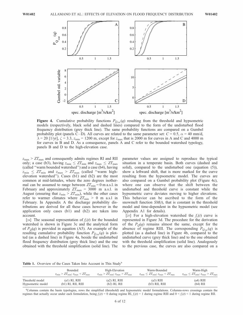
watershed is shown in Figure 3c and the analytical formof PQ(q) is provided in equation (A5). An example of theresulting cumulative probability function PQAM

(q) is plot-ted (as a dashed line) in Figure 4a, beside the undisturbedflood frequency distribution (grey thick line) and the oneobtained with the threshold simplification (solid line). The

parameter values are assigned to reproduce the typicalsituation in a temperate basin. Both curves (dashed andsolid), compared to the undisturbed one (equation (5)),show a leftward shift, that is more marked for the curveresulting from the hypsometric model. The curves arealso compared on a Gumbel probability plot (Figure 4c),where one can observe that the shift between theundisturbed and threshold curve is constant while thehypsometric curve deviates moving to higher elevations.This behavior can be ascribed to the form of thesnowmelt function SM(t), that is constant in the thresholdmodel and time-dependent in the hypsometric model (seeAppendix A1 for details).[25] For a high-elevation watershed the fc(t) curve is

represented in Figure 3d. The procedure for the derivationof the PQ(q) remains almost the same, except for theabsence of regime RIII. The corresponding PQAM

(q) isplotted (as a dashed line) in Figure 4b, compared to theundisturbed curve (grey thick line) and to the one obtainedwith the threshold simplification (solid line). Analogouslyto the previous case, the curves are also compared on a

Table 1. Overview of the Cases Taken Into Account in This Studya

Boundedzmin > ZTmin; zmax < ZTmax

High-Elevationzmin > ZTmin; zmax > ZTmax

Warm-Boundedzmin � ZTmin; zmax < ZTmax

Warm-Highzmin � ZTmin; zmax > ZTmax

Threshold model (a1) RI, RIII (a2) RI, RIII (a3) RIII (a4) RIIIHypsometric model (b1) RI, RII, RIII (b2) RI, RII (b3) RII, RIII (b4) RII

aColumns contain the basin typologies, rows the simplified (threshold) and hypsometric model formulations. Columns-rows crossings contain theregimes that actually occur under each formulation, being fc(t) = 0 during regime RI, fc(t) = 1 during regime RIII and 0 < fc(t) < 1 during regime RII.

Figure 4. Cumulative probability functions PQAM(q) resulting from the threshold and hypsometric

models (respectively, black solid and dashed lines) compared to the form of the undisturbed floodfrequency distribution (grey thick line). The same probability functions are compared on a Gumbelprobability plot (panels C–D). All curves are related to the same parameter set: C = 0.5, a = 40 mm/d,l = 20 [1/yr], z = 3.3, zmin = 1200 m, except for zmax that is 2000 m for curves in A and C and 4000 mfor curves in B and D. As a consequence, panels A and C refer to the bounded watershed typology,panels B and D to the high-elevation case.

6 of 12

W01402 ALLAMANO ET AL.: EFFECTS OF ELEVATION ON FLOOD FREQUENCY DISTRIBUTION W01402

Gumbel probability plot (Figure 4d) where a more markedshift than in the bounded watershed case is observed.

4. Model Sensitivity

[26] In this section the attitude of the model to representrealistically flood processes in mountainous basins is ex-plored using ‘‘synthetic’’ case-studies, identified by differ-ent parameter sets that trace back to the cases of boundedand high-elevation watersheds (see Table 1 for an overviewof all the possible cases). In general the following classes ofparameters have to be specified:[27] (1) Geometric parameters, describing watershed

hypsometry, such as the maximum (zmax) and minimum(zmin) elevations of the watershed and the parameter zcontrolling the shape of the hypsometric curve. z results

from the equivalence between the integral of the hypsomet-ric curve and the normalized mean watershed elevation.[28] (2) Climatic parameters at the basin scale, i.e. a and

l for the rainfall model and the total annual rainfall R. Tokeep the analytical tractability of the model we assume aand l to be constant all over the year. The introduction of aseasonal regime of a and l, in fact, would be more realisticbut would make the model much more complicated. Wealso assume R to be proportional to a through a parameter k,so that a becomes the scale parameter of the model.[29] (3) Climatic parameters related to the macro-region,

such as the maximum (ZTmax) and minimum (ZTmin) valuesof the freezing level migration curve. Observe that bysetting the two limits on the ZT(t) one assumes that thetemperature regime of the region has already been trans-posed into the freezing level curve. This is done using aconstant temperature lapse rate (that usually ranges between5� 7�C every 1000 m of elevation).[30] In our analysis, the degrees of freedom of the

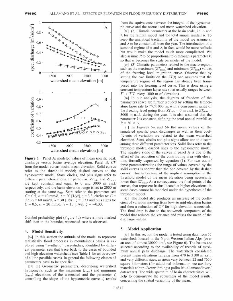
parameters space are further reduced by setting the temper-ature lapse rate to 7�C/1000 m, with a consequent range ofthe freezing level going from ZTmin = 0 m a.s.l. to ZTmax =3000 m a.s.l. during the year. It is also assumed that theparameter k is constant, defining the total annual rainfall asR = 30 � a.[31] In Figures 5a and 5b the mean values of the

simulated specific peak discharges as well as their coef-ficients of variation are related to the mean watershedelevation. Stars, circles and plus signs allow one to discernamong three different parameter sets. Solid lines refer to thethreshold model, dashed lines to the hypsometric model.The negative slope of the curves in panel A is due to theeffect of the reduction of the contributing area with eleva-tion, formally expressed by equation (1). For two out ofthree parameterizations the range of values covered by thesolid curves is shorter than the one covered by the dashedcurves. This is because of the implicit assumption in thethreshold model of the mean elevation being necessarilylower than ZTmax. As a consequence, the final points of thecurves, that represent basins located at higher elevations, insome cases cannot be modeled under the hypotheses of thethreshold model.[32] The model also produces an increase of the coeffi-

cient of variation moving from low- to mid-elevation basinsand then a reduction of CV for high-elevation watersheds.The final drop is due to the snowmelt component of themodel that reduces the variance and raises the mean of thedischarge values.

5. Model Application

[33] In this section the model is tested using data from 57watersheds located in the North-Western Italian Alps (overan area of almost 30000 km2, see Figure 6). The basins areselected according to the availability of records of maxi-mum annual peak discharge. The watersheds consideredpresent mean elevations ranging from 470 to 3100 m a.s.l.and very different sizes, as areas vary between 22 and 7650square kilometers (for additional information see auxiliarymaterials at http://www.idrologia.polito.it/ allamano/lavori/dataset.txt). The wide spectrum of basin characteristics willhelp to demonstrate the robustness of the model results,concerning the spatial variability of the mean.

Figure 5. Panel A: modeled values of mean specific peakdischarge versus basins average elevation. Panel B: CVfrom the model versus basins mean elevation. Solid curvesrefer to the threshold model; dashed curves to thehypsometric model. Stars, circles, and plus signs refer todifferent parameterizations. In particular, ZTmin and ZTmax

are kept constant and equal to 0 and 3000 m a.s.l.respectively, and the basin elevation range is set to 2000 mstarting at the same zmin. Stars refer to the parameter set:C = 0.5, a = 40 mm/d, l = 20 [1/yr], z = 3.3, circles to: C =0.5, a = 60 mm/d, l = 30 [1/yr], z = 0.33 and plus signs to:C = 0.5, a = 20 mm/d, l = 10 [1/yr], z = �0.33.

W01402 ALLAMANO ET AL.: EFFECTS OF ELEVATION ON FLOOD FREQUENCY DISTRIBUTION

7 of 12

W01402

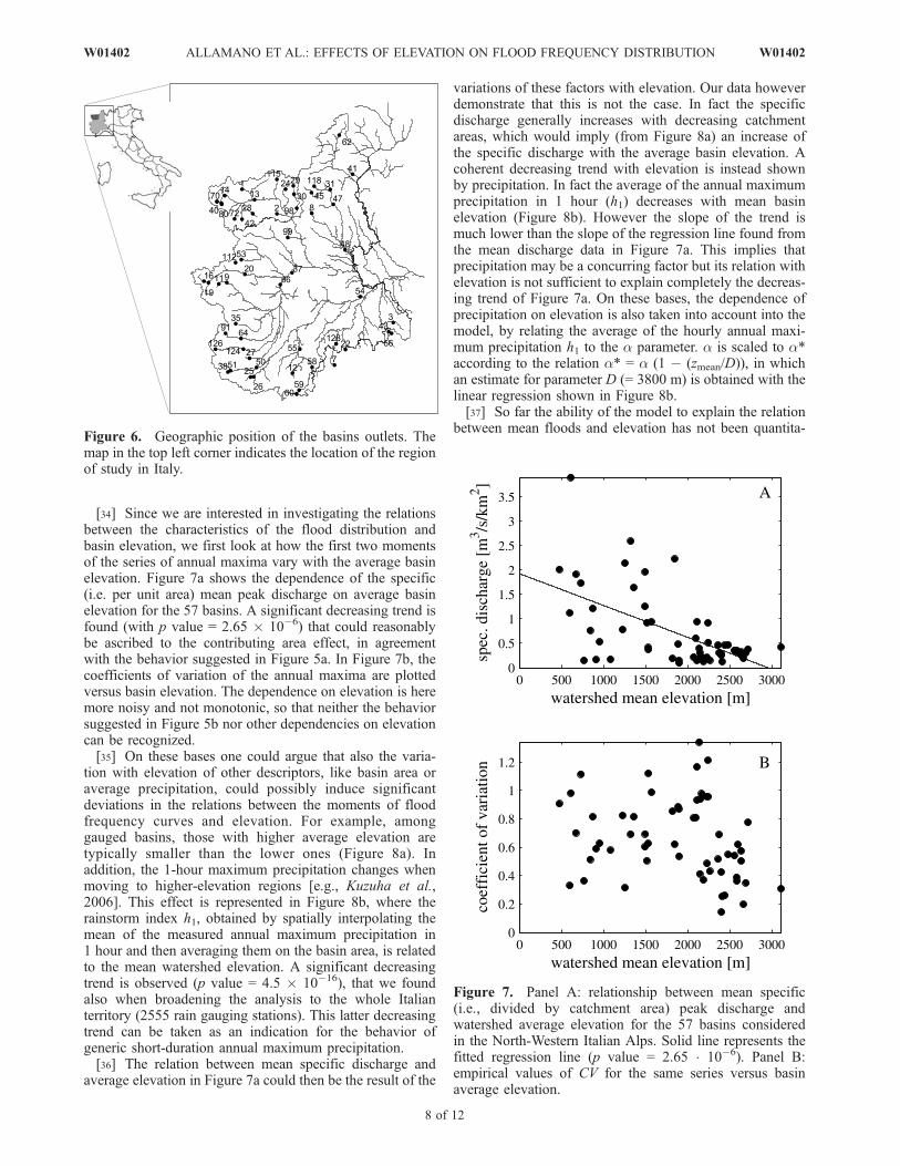
[34] Since we are interested in investigating the relationsbetween the characteristics of the flood distribution andbasin elevation, we first look at how the first two momentsof the series of annual maxima vary with the average basinelevation. Figure 7a shows the dependence of the specific(i.e. per unit area) mean peak discharge on average basinelevation for the 57 basins. A significant decreasing trend isfound (with p value = 2.65 � 10�6) that could reasonablybe ascribed to the contributing area effect, in agreementwith the behavior suggested in Figure 5a. In Figure 7b, thecoefficients of variation of the annual maxima are plottedversus basin elevation. The dependence on elevation is heremore noisy and not monotonic, so that neither the behaviorsuggested in Figure 5b nor other dependencies on elevationcan be recognized.[35] On these bases one could argue that also the varia-

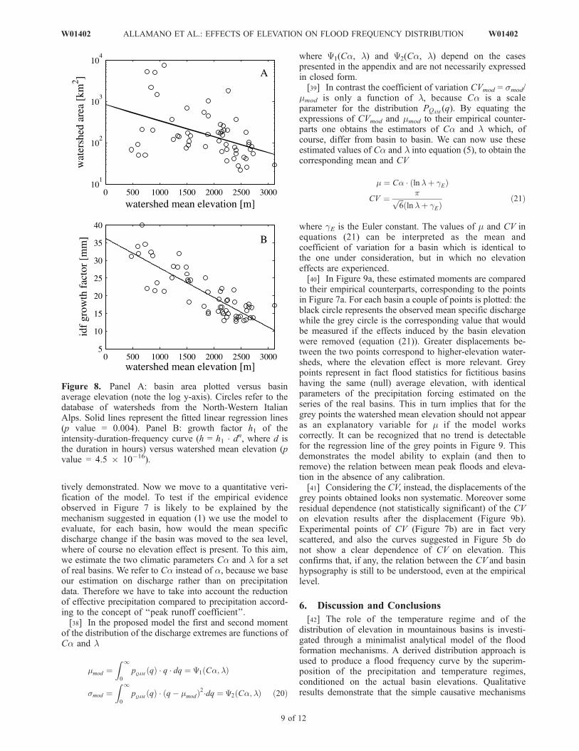
tion with elevation of other descriptors, like basin area oraverage precipitation, could possibly induce significantdeviations in the relations between the moments of floodfrequency curves and elevation. For example, amonggauged basins, those with higher average elevation aretypically smaller than the lower ones (Figure 8a). Inaddition, the 1-hour maximum precipitation changes whenmoving to higher-elevation regions [e.g., Kuzuha et al.,2006]. This effect is represented in Figure 8b, where therainstorm index h1, obtained by spatially interpolating themean of the measured annual maximum precipitation in1 hour and then averaging them on the basin area, is relatedto the mean watershed elevation. A significant decreasingtrend is observed (p value = 4.5 � 10�16), that we foundalso when broadening the analysis to the whole Italianterritory (2555 rain gauging stations). This latter decreasingtrend can be taken as an indication for the behavior ofgeneric short-duration annual maximum precipitation.[36] The relation between mean specific discharge and

average elevation in Figure 7a could then be the result of the

variations of these factors with elevation. Our data howeverdemonstrate that this is not the case. In fact the specificdischarge generally increases with decreasing catchmentareas, which would imply (from Figure 8a) an increase ofthe specific discharge with the average basin elevation. Acoherent decreasing trend with elevation is instead shownby precipitation. In fact the average of the annual maximumprecipitation in 1 hour (h1) decreases with mean basinelevation (Figure 8b). However the slope of the trend ismuch lower than the slope of the regression line found fromthe mean discharge data in Figure 7a. This implies thatprecipitation may be a concurring factor but its relation withelevation is not sufficient to explain completely the decreas-ing trend of Figure 7a. On these bases, the dependence ofprecipitation on elevation is also taken into account into themodel, by relating the average of the hourly annual maxi-mum precipitation h1 to the a parameter. a is scaled to a*according to the relation a* = a (1 � (zmean/D)), in whichan estimate for parameter D (= 3800 m) is obtained with thelinear regression shown in Figure 8b.[37] So far the ability of the model to explain the relation

between mean floods and elevation has not been quantita-Figure 6. Geographic position of the basins outlets. Themap in the top left corner indicates the location of the regionof study in Italy.

Figure 7. Panel A: relationship between mean specific(i.e., divided by catchment area) peak discharge andwatershed average elevation for the 57 basins consideredin the North-Western Italian Alps. Solid line represents thefitted regression line (p value = 2.65 � 10�6). Panel B:empirical values of CV for the same series versus basinaverage elevation.

8 of 12

W01402 ALLAMANO ET AL.: EFFECTS OF ELEVATION ON FLOOD FREQUENCY DISTRIBUTION W01402

tively demonstrated. Now we move to a quantitative veri-fication of the model. To test if the empirical evidenceobserved in Figure 7 is likely to be explained by themechanism suggested in equation (1) we use the model toevaluate, for each basin, how would the mean specificdischarge change if the basin was moved to the sea level,where of course no elevation effect is present. To this aim,we estimate the two climatic parameters Ca and l for a setof real basins. We refer to Ca instead of a, because we baseour estimation on discharge rather than on precipitationdata. Therefore we have to take into account the reductionof effective precipitation compared to precipitation accord-ing to the concept of ‘‘peak runoff coefficient’’.[38] In the proposed model the first and second moment

of the distribution of the discharge extremes are functions ofCa and l

mmod ¼Z 1

0

pQAM

qð Þ � q � dq ¼ Y1 Ca;lð Þ

smod ¼Z 1

0

pQAM

qð Þ � q� mmodð Þ2�dq ¼ Y2 Ca;lð Þ ð20Þ

where Y1(Ca, l) and Y2(Ca, l) depend on the casespresented in the appendix and are not necessarily expressedin closed form.[39] In contrast the coefficient of variation CVmod = smod/

mmod is only a function of l, because Ca is a scaleparameter for the distribution PQAM

(q). By equating theexpressions of CVmod and mmod to their empirical counter-parts one obtains the estimators of Ca and l which, ofcourse, differ from basin to basin. We can now use theseestimated values of Ca and l into equation (5), to obtain thecorresponding mean and CV

m ¼ Ca � lnlþ gEð Þ

CV ¼ pffiffiffi6

plnlþ gEð Þ

ð21Þ

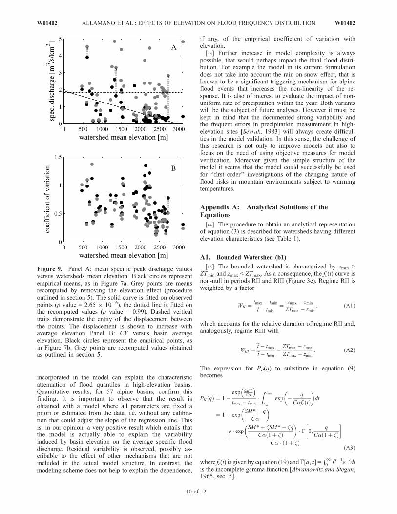
where gE is the Euler constant. The values of m and CV inequations (21) can be interpreted as the mean andcoefficient of variation for a basin which is identical tothe one under consideration, but in which no elevationeffects are experienced.[40] In Figure 9a, these estimated moments are compared

to their empirical counterparts, corresponding to the pointsin Figure 7a. For each basin a couple of points is plotted: theblack circle represents the observed mean specific dischargewhile the grey circle is the corresponding value that wouldbe measured if the effects induced by the basin elevationwere removed (equation (21)). Greater displacements be-tween the two points correspond to higher-elevation water-sheds, where the elevation effect is more relevant. Greypoints represent in fact flood statistics for fictitious basinshaving the same (null) average elevation, with identicalparameters of the precipitation forcing estimated on theseries of the real basins. This in turn implies that for thegrey points the watershed mean elevation should not appearas an explanatory variable for m if the model workscorrectly. It can be recognized that no trend is detectablefor the regression line of the grey points in Figure 9. Thisdemonstrates the model ability to explain (and then toremove) the relation between mean peak floods and eleva-tion in the absence of any calibration.[41] Considering the CV, instead, the displacements of the

grey points obtained looks non systematic. Moreover someresidual dependence (not statistically significant) of the CVon elevation results after the displacement (Figure 9b).Experimental points of CV (Figure 7b) are in fact veryscattered, and also the curves suggested in Figure 5b donot show a clear dependence of CV on elevation. Thisconfirms that, if any, the relation between the CV and basinhypsography is still to be understood, even at the empiricallevel.

6. Discussion and Conclusions

[42] The role of the temperature regime and of thedistribution of elevation in mountainous basins is investi-gated through a minimalist analytical model of the floodformation mechanisms. A derived distribution approach isused to produce a flood frequency curve by the superim-position of the precipitation and temperature regimes,conditioned on the actual basin elevations. Qualitativeresults demonstrate that the simple causative mechanisms

Figure 8. Panel A: basin area plotted versus basinaverage elevation (note the log y-axis). Circles refer to thedatabase of watersheds from the North-Western ItalianAlps. Solid lines represent the fitted linear regression lines(p value = 0.004). Panel B: growth factor h1 of theintensity-duration-frequency curve (h = h1 � dn, where d isthe duration in hours) versus watershed mean elevation (pvalue = 4.5 � 10�16).

W01402 ALLAMANO ET AL.: EFFECTS OF ELEVATION ON FLOOD FREQUENCY DISTRIBUTION

9 of 12

W01402

incorporated in the model can explain the characteristicattenuation of flood quantiles in high-elevation basins.Quantitative results, for 57 alpine basins, confirm thisfinding. It is important to observe that the result isobtained with a model where all parameters are fixed apriori or estimated from the data, i.e. without any calibra-tion that could adjust the slope of the regression line. Thisis, in our opinion, a very positive result which entails thatthe model is actually able to explain the variabilityinduced by basin elevation on the average specific flooddischarge. Residual variability is observed, possibly as-cribable to the effect of other mechanisms that are notincluded in the actual model structure. In contrast, themodeling scheme does not help to explain the dependence,

if any, of the empirical coefficient of variation withelevation.[43] Further increase in model complexity is always

possible, that would perhaps impact the final flood distri-bution. For example the model in its current formulationdoes not take into account the rain-on-snow effect, that isknown to be a significant triggering mechanism for alpineflood events that increases the non-linearity of the re-sponse. It is also of interest to evaluate the impact of non-uniform rate of precipitation within the year. Both variantswill be the subject of future analyses. However it must bekept in mind that the documented strong variability andthe frequent errors in precipitation measurement in high-elevation sites [Sevruk, 1983] will always create difficul-ties in the model validation. In this sense, the challenge ofthis research is not only to improve models but also tofocus on the need of using objective measures for modelverification. Moreover given the simple structure of themodel it seems that the model could successfully be usedfor ‘‘first order’’ investigations of the changing nature offlood risks in mountain environments subject to warmingtemperatures.

Appendix A: Analytical Solutions of theEquations

[44] The procedure to obtain an analytical representationof equation (3) is described for watersheds having differentelevation characteristics (see Table 1).

A1. Bounded Watershed (b1)

[45] The bounded watershed is characterized by zmin >ZTmin and zmax < ZTmax. As a consequence, the fc(t) curve isnon-null in periods RII and RIII (Figure 3c). Regime RII isweighted by a factor

WII ¼tmax � tminet � tmin

¼ zmax � zmin

ZTmax � zmin

; ðA1Þ

which accounts for the relative duration of regime RII and,analogously, regime RIII with

WIII ¼et � tmaxet � tmin

¼ ZTmax � zmax

ZTmax � zmin

: ðA2Þ

The expression for PII(q) to substitute in equation (9)becomes

PII qð Þ ¼ 1�exp SM*

Ca

� �tmax � tmin

�Z tmax

tmin

exp � q

Cafc tð Þ

� �dt

¼ 1� expSM*� q

Ca

� �

þq � exp SM*þ zSM*� zq

Ca 1þ zð Þ

� �� G 0;

q

Ca 1þ zð Þ

� �Ca � 1þ zð Þ

ðA3Þ

where fc(t) is given by equation (19) andG[a, z] =R10

ta�1e�tdtis the incomplete gamma function [Abramowitz and Stegun,1965, sec. 5].

Figure 9. Panel A: mean specific peak discharge valuesversus watersheds mean elevation. Black circles representempirical means, as in Figure 7a. Grey points are meansrecomputed by removing the elevation effect (procedureoutlined in section 5). The solid curve is fitted on observedpoints (p value = 2.65 � 10�6), the dotted line is fitted onthe recomputed values (p value = 0.99). Dashed verticaltraits demonstrate the entity of the displacement betweenthe points. The displacement is shown to increase withaverage elevation Panel B: CV versus basin averageelevation. Black circles represent the empirical points, asin Figure 7b. Grey points are recomputed values obtainedas outlined in section 5.

10 of 12

W01402 ALLAMANO ET AL.: EFFECTS OF ELEVATION ON FLOOD FREQUENCY DISTRIBUTION W01402

[46] Using equation (12) the SM* factor is obtained as

SM* ¼ R

365� �ð�z� �BÞ � ð1þ �Þ�z ln½1þ ���ð�D��zÞ þ ð1þ �Þ�z ln½1þ �� ; ðA4Þ

w h e r e �z ¼ ðzmax � zminÞ, B ¼ ðzmin � ZTminÞ a n dD ¼ ðzmin � ZTmaxÞ. By introducing equations (13), (A1),(A2), (A3) and (A4) in equation (9) one finds

PQ qð Þ ¼ 1� expSM*� q

C�

� �

�exp

SM*ð1þ �Þ � �q

C�ð1þ �Þ

� �� q�z � � 0; q

C�ð1þ�Þ

h iC� � Dð1þ �Þ : ðA5Þ

To obtain the distribution of the extremes, one shouldreplace the term PQ(q) of (A5) in equation (4), whereequation (10) should be used to account for the effects ofregime RI on the reduction of l.

A2. High-Elevation Watershed (b2)

[47] For a high-elevation watershed (having zmin > ZTmin,zmax > ZTmax) the procedure for the derivation of PQ(q)remains almost the same, except for the absence ofregime RIII (Figure 3d). This absence changes theintegration interval in equations (12) and (A3) into[tmin � et] and allows one to obtain, by analyticalintegration

SM* ¼ � R

3651þ �2 ��ZT=ð1þ �Þ

�D� 2�z � ATh � �Dð�D�2�z

h i0@ 1A; ðA6Þ

where D is as previously defined, �ZT ¼ ðZTmax � ZTminÞand ATh[�] is the hyperbolic arc-tangent.[48] The expression of PQ(q) is therefore

PQðqÞ ¼ 1� expqð�Z � �DÞð1þ �ÞD=C�þ SM*

C�

� �� q�z

C�ð1þ �ÞD

� exp SM*ð1þ �Þ � q�

C�ð1þ �Þ

� �� EI 1;� q�z

C�ð1þ �ÞD

� �; ðA7Þ

where EI[n, z] =R11(e�zt/tn)dt is the exponential integral

function [Abramowitz and Stegun, 1965, sec. 6]. In order toobtain the distribution of the extremes, equation (A7)should be substituted into equation (4), again taking intoaccount the reduction of l (equation (10)).

A3. Warm Bounded Watershed (b3)

[49] In warmer climates, where in February ZTmin > 0, thewarm counterpart of the bounded watershed b1 should beconsidered. This is the case of a watershed having zmin �ZTmin and zmax < ZTmax, in which case one obtains:

SM* ¼ R

365

�2�ZT

�ðGþ ��ZTÞ � ð1þ �Þ�z lnð1þ�Þ�z

�zþ�ðzminþZTminÞ

h i� 1

0@ 1A;

ðA8Þ

where G ¼ ðzmax � ZTminÞ and

PQðqÞ ¼expð�q=C�Þ

C�ð1þ �Þ�ZT

C�ð1þ �Þ exp � ZTminq

C�ð1þ �ÞB

� ���exp

ZTminq

C�ð1� �ÞBþ SM*

C�

� �þ D exp

q

C�1þ ZTmin

Bð1þ �Þ

� �� ���ZT � B exp

zmaxq

C�ð1þ �ÞBþ SM*

C�

� ��� exp z

qþ SM*ð1þ �ÞC�ð1þ �Þ

� ���zq

EI½�qC�ð1þ �Þ� � EI

"�zq

C�ð1þ �ÞB

#!!: ðA9Þ

A4. Warm High-Elevation Watershed (b4)

[50] Analogously, for the warm high-elevation case(having zmin � ZTmin, zmax > ZTmax), one has

SM* ¼ R

365

�2�ZT=ð1þ �Þ��ZT þ 2�zATh ���ZT

2�z��ð2zmin��ZTÞ

h i� 1

0@ 1A; ðA10Þ

and

PQðqÞ ¼ 1�exp SM*

C� � qC�ð1þ1=�Þ

� �C�ð1þ �Þ�ZT

ð�C�ð1þ �ÞÞ

��� D exp

�zq

C�ð1þ �ÞD � B exp�zq

C�ð1� �ÞD

����þ q�z

�EI

��zq

C�ð1� �ÞD � EI�zq

C�ð1� �ÞD

� �� ��:

ðA11Þ

[51] Acknowledgments. The work was funded by the Italian Ministryof Education (grants 2005080287 and 2006089189). Comments andsuggestions from D. P. Lettenmaier, R. Woods, A. F. Hamlet, Y. Alilaand two anonymous reviewers are gratefully acknowledged.

ReferencesAbramowitz, M., and I. Stegun (1965),Handbook of Mathematical Functions,Applied Math. Ser. 55, National Bureau of Standards, Dover Publications,New York.

Alila, Y., and A. Mtiraoui (2002), Implications of heterogeneous flood-frequency distributions on traditional stream-discharge prediction techni-ques, Hydrol. Processes, 16, 1065–1084.

Ambroise, A. (2004), Variable ‘‘active’’ versus ‘‘contributing’’ areas peri-ods: A necessary distinction, Hydrol. Processes, 18, 1149–1155.

Bacchi, B., and R. Ranzi (2003), Hydrological and meteorological aspects offloods in the Alps: An overview, Hydrol. Earth Syst. Sci., 7(6), 785–798.

Bloschl, G., and M. Sivapalan (1997), Process controls on regional floodfrequency: Coefficient of variation and basin scale, Water Resour. Res.,33(12), 2967–2980.

Buishand, T., and G. Demare (1990), Estimation of the annual maximumdistribution from samples of maxima in separate seasons, StochasticHydrol. Hydraul., 4, 89–103.

Coles, S. (2001), An Introduction to Statistical Modeling of Extreme Values,Springer Series in Statistics, Springer-Verlag, London, U.K.

De Michele, C., and G. Salvadori (2002), On the derived flood frequencydistribution: Analytical formulation and the influence of antecedent soil

W01402 ALLAMANO ET AL.: EFFECTS OF ELEVATION ON FLOOD FREQUENCY DISTRIBUTION

11 of 12

W01402

moisture condition, J. Hydrol., 262, 245–258.Eagleson, P. (1972), Dynamics of flood frequency,Water Resour. Res., 8(4),878–898.

Eagleson, P. (1978), Climate, soil and vegetation. 1. Introduction to waterbalance dynamics, Water Resour. Res., 14(5), 705–712.

Gottschalk, L., and R. Weingartner (1998), Distribution of peak flow de-rived from a distribution of rainfall volume and runoff coefficient, and aunit hydrograph, J. Hydrol., 208, 148–162.

Iacobellis, V., and M. Fiorentino (2000), Derived distribution of floodsbased on the concept of partial area coverage with a climatic appeal,Water Resour. Res., 36(2), 469–482.

Kuzuha, Y., M. Sivapalan, K. Tomosugi, T. Kishii, and Y. Komatsu (2006),Role of the spatial variability of rainfall intensity: Improvement ofEagleson’s classical model to explain the relationship between the coef-ficient of variation of annual maximum discharge and catchment size,Hydrol. Processes, 20, 1335–1346.

Littlewood, I. (Ed.) (2002), Continuos River Flow in Simulation: Methods,Applications and Uncertainties, Occasional Paper 13, British Hydrol.Soc., U.K.

Loukas, A. (2002), Flood frequency estimation by a derived distributionprocedure, J. Hydrol., 255, 69–89.

Loukas, A., L. Vasiliades, and N. Dalezios (2000), Flood producing me-chanisms identification in southern British Columbia, Canada, J. Hydrol.,227, 218–235.

Merz, R., and G. Bloschl (2003), A process typology of regional floods,Water Resour. Res., 39(12), 1340, doi:10.1029/2002WR001952.

Milly, P. (1994a), Climate, interseasonal storage of soil water, and theannual water balance, Adv. Water Resour., 17, 19–24.

Milly, P. (1994b), Climate, soil water storage and the average annual waterbalance, Water Resour. Res., 30(7), 2143–2156.

Perona, P., A. Porporato, and L. Ridolfi (2007), A stochastic process for theinterannual snow storage and melting dynamics, J. Geophys. Res., 112,D08107, doi:10.1029/2006JD007798.

Rahman, A., P. Weinmann, T. Hoang, and E. Laurenson (2002), Monte Carlosimulation of flood frequency curves from rainfall, J. Hydrol., 256(3–4),196–210.

Rodriguez Iturbe, I., A. Porporato, F. Laio, and L. Ridolfi (2001), Plants inwater-controlled ecosystems: Active role in hydrologic processes andresponse to water stress I. Scope and general outline, Adv. Water Resour.,24, 695–705.

Ross, S. (1996), Stochastic Processes, John Wiley, New York.Rossi, F., M. Fiorentino, and P. Versace (1984), Two-component extremevalue distribution for flood frequency analysis,Water Resour. Res., 20(7),847–856.

Sevruk, B. (1983), Correction of measured precipitation in the Alps usingthe water equivalent of new snow, Nord. Hydrol., 14(2), 49–58.

Singh, V., S. Wang, and L. Zhang (2005), Frequency analysis of noniden-tically distributed hydrologic flood data, J. Hydrol., 307, 175–195.

Sivapalan, M., G. Bloschl, R. Merz, and D. Gutknecht (2005), Linking floodfrequency to long-term water balance: Incorporating effects of seasonality,Water Resour. Res., 41, W06012, doi:10.1029/2004WR003439.

Strahler, A. (1952), Hypsometric (area-altitude) analysis of erosional topo-graphy, Bull. Geol. Soc. Am., 63, 1117–1142.

Waylen, P., and M. Woo (1982), Prediction of annual floods generated bymixed processes, Water Resour. Res., 18(4), 1283–1286.

Wood, E., and C. Hebson (1986), On hydrologic similarity: 1. Derivation ofthe dimensionless flood frequency curve, Water Resour. Res., 22(11),1549–1554.

Woods, R. (2003), The relative roles of climate, soil, vegetation and topo-graphy in determining seasonal and long-term catchment dynamics, Adv.Water Resour., 26(3), 295–309.

����������������������������P. Allamano, P. Claps, and F. Laio, Dipartimento di Idraulica, Trasporti

ed Infrastrutture Civili, Politecnico di Torino, Corso Duca degli Abruzzi,24, I-10129 Torino, Italy. (paola.allamano@polito.it)

12 of 12

W01402 ALLAMANO ET AL.: EFFECTS OF ELEVATION ON FLOOD FREQUENCY DISTRIBUTION W01402