For Peer Review

AN ANALYSIS OF COUNT DATA MODELS FOR THE STUDY OF EXCLUSIVITY IN WINE CONSUMPTION

Journal: Applied Economics Manuscript ID: APE-06-0238.R1

Journal Selection: Applied Economics

JEL Code:C25 - Discrete Regression and Qualitative Choice Models < C2 - Econometric Methods: Single Equation Models < C - Mathematical and Quantitative Methods, Q13 - Agricultural Markets and Marketing|Cooperatives|Agribusiness < Q1 - Agriculture < Q - Agricultural and Natural Resource Economics

Keywords: Count data models, Poisson regression model, Negative Binomial regression models, finite mixture models, number of wine types

Editorial Office, Dept of Economics, Warwick University, Coventry CV4 7AL, UK

Submitted Manuscriptpe

er-0

0582

114,

ver

sion

1 -

1 Ap

r 201

1Author manuscript, published in "Applied Economics 41, 12 (2009) 1563-1574"

DOI : 10.1080/00036840601032227

For Peer Review

AN ANALYSIS OF COUNT DATA MODELS FOR THE STUDY OF EXCLUSIVITY IN WINE CONSUMPTION

Víctor Javier Cano Fernández; Ginés Guirao Pérez; María Carolina Rodríguez Donate y Margarita Esther Romero Rodríguez

Departamento de Economía de las Instituciones, Estadística Económica y

Econometría Universidad de La Laguna. Campus de Guajara, Camino la Hornera, s/n, 38071,

Tenerife, Islas Canarias, España cdonate@ull.es

Abstract

Several models which analyze count data have been proposed in econometric

literature. These models allow the discrete, non-negative nature of specific

phenomena of interest to be gathered in a appropriate way and can be useful for the

explanation of specific preference structures among individuals. In this work, an

analysis of the number of wine types consumed by residents of Tenerife is carried

out, with an aim to observe which characteristics determine the exclusivity in its

consumption, given the current context of increased competition in this sector. The

specific characteristics of the considered variable allow the study to cover two

aspects. The first is methodological, and is seen by the variety of models that may be

considered in this case. This focus consists in comparing several possibilities which

fit the type of count data involved. The second aspect is clearly empirical, and is

based on the description of not only the most appropriate decision-making

mechanism for the study but in the identification of those factors that explain the

diversity in wine consumption.

Keywords: Count data models, Poisson regression model, Negative Binomial regression models, finite

mixture models, number of wine types.

Page 1 of 26

Editorial Office, Dept of Economics, Warwick University, Coventry CV4 7AL, UK

Submitted Manuscript

123456789101112131415161718192021222324252627282930313233343536373839404142434445464748495051525354555657585960

peer

-005

8211

4, v

ersi

on 1

- 1

Apr 2

011

For Peer Review

2

1. Introduction

The worldwide wine scene has gone through significant changes lately, especially

since the 90´s. Both producers and wine drinkers have taken turns as the main actors

in these changes. The most significant event with respect to demand has been a

decrease in worldwide wine consumption, or at least a certain amount of stagnation

as a consequence of two opposite effects. On one hand, the increase in demand in

countries with traditionally low wine consumption, and the other, a reduction of

observed per-capita consumption in those countries where indeed there is greater

wine production and tendency to drink wine.

Life style changes have followed a parallel path. For instance, now an increase has

been observed in the consumption of higher quality wines than before. Changes have

also taken place in traditional family events and social occasions in general, where

once daily wine consumption was typical but now has been replaced by an

occasional status.

The supply side has also undergone changes. The international players have

witnessed the entrance of new countries in a sharing role in two systems of

harvesting, production, and commercialization. The first model belongs to the Old

World countries and includes France, Italy, Germany, Portugal and Spain. A second

type is made up of the New World countries, of which Australia, South Africa, Chile,

Argentina and the United States are the major players. As a result there is saturation

in the international wine market. The slowdown in demand is accompanied by an

increase in the supply of quality wines. And in this environment of increasing

competition many wine producers have sensed the need to construct their own image

and create a concept of quality that can be perceived by consumers.

Page 2 of 26

Editorial Office, Dept of Economics, Warwick University, Coventry CV4 7AL, UK

Submitted Manuscript

123456789101112131415161718192021222324252627282930313233343536373839404142434445464748495051525354555657585960

peer

-005

8211

4, v

ersi

on 1

- 1

Apr 2

011

For Peer Review

3

This scenario can even be introduced, with certain overtones, to the Canary

Archipelago, and specifically to the island of Tenerife. Vineyards and the wine

community arouse analytical interest in this geographical area not only because of its

tradition in the wine production process –present in the Archipelago since the

1400´s- but also because of the inherent peculiarity of these wines, namely the

climatic conditions, the orography in the island, and the variety of grapes used1. Vine

growing is also an important asset of undeniable ecological value given its

contribution to rural developments, one of the selling points for tourism on the

island, which is the true motor of economic activity in the Archipelago.

Increased competition in the wine market, in addition to recent trends defined by

consumers, such as the drop in per capita wine consumption and an increase in the

demand by consumers for quality wines, have motivated the need for detailed studies

regarding consumer behaviour. But these studies need to go beyond such questions

as explaining the quantity or frequency of wine consumption, and must include the

ways and means in which it is occurring. The characteristics that define the place of

consumption or purchase, the origin or region from which the wine came from, and

the brand or wine types, can be important when helping develop strategies to

sufficiently differentiate wines under current circumstances. Some research indicates

that it is difficult to obtain an appropriate economic forecast in the wine sector

without a thorough study of demand. Either way it is possible to undertake a study of

consumer behaviour using several approaches given the importance that brand

loyalty has had in prior research.

This study recognizes the limited amount of available information in this regard. We

1 A significant amount of grape diversity is present in the Canary Archipelago, due to several reasons, one of which is the absence of phylloxera.

Page 3 of 26

Editorial Office, Dept of Economics, Warwick University, Coventry CV4 7AL, UK

Submitted Manuscript

123456789101112131415161718192021222324252627282930313233343536373839404142434445464748495051525354555657585960

peer

-005

8211

4, v

ersi

on 1

- 1

Apr 2

011

For Peer Review

4

therefore choose an approach not based strictly on one dimension but instead adopt a

view which will at least allow us to observe consumption behaviour based on

exclusivity or diversity. The study specifically aims to describe the socio-economic

characteristics which best define the number of different wine types consumed by

individuals based on a survey carried out with residents from the island of Tenerife2.

In our case a special type of model is necessary to properly gather the characteristics

of the phenomenon that is being explained, namely its discrete and non-negative

nature. Several alternatives have been proposed in the econometric literature which

can fall under the term count data regression models. These models allow us to

undertake this type of analysis and also offer some alternatives when defining the

structure of consumer preference.

The specific characteristics of this variable allow the study to cover two aspects. The

first concerns methodology, which is evident by the variety of models that can be

utilized and consists in comparing the alternatives which fit the type of count that is

found. The second is eminently empirical, and its goal is to describe not only the

most suitable decision making process but to identify which factors explain the

increased or decreased diversity in wine consumption.

Given these objectives, the paper is divided into three sections. The first section

develops the methodology used, including the different models, noting the most

advantageous features of each. Section two describes the data and compares the

obtained results from all the models used. The last section draws the most relevant

conclusions.

2 Several studies which analyze the influence of socioeconomic characteristics on alcohol consumption are Nayga (1996), Su and Yen (2000) and Selvanathan and Selvanathan (2004).

Page 4 of 26

Editorial Office, Dept of Economics, Warwick University, Coventry CV4 7AL, UK

Submitted Manuscript

123456789101112131415161718192021222324252627282930313233343536373839404142434445464748495051525354555657585960

peer

-005

8211

4, v

ersi

on 1

- 1

Apr 2

011

For Peer Review

5

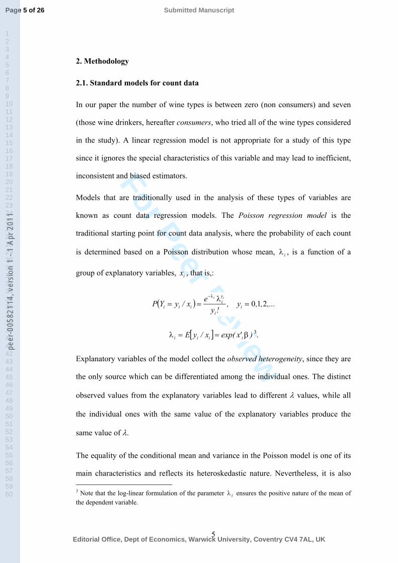
2. Methodology

2.1. Standard models for count data

In our paper the number of wine types is between zero (non consumers) and seven

(those wine drinkers, hereafter consumers, who tried all of the wine types considered

in the study). A linear regression model is not appropriate for a study of this type

since it ignores the special characteristics of this variable and may lead to inefficient,

inconsistent and biased estimators.

Models that are traditionally used in the analysis of these types of variables are

known as count data regression models. The Poisson regression model is the

traditional starting point for count data analysis, where the probability of each count

is determined based on a Poisson distribution whose mean, iλ , is a function of a

group of explanatory variables, ix , that is,:

( ) ,...,,y,!y

ex/yYP ii

yi

iii

ii

210=λ

==λ−

[ ] )'xexp(x/yE iiii β==λ 3.

Explanatory variables of the model collect the observed heterogeneity, since they are

the only source which can be differentiated among the individual ones. The distinct

observed values from the explanatory variables lead to different λ values, while all

the individual ones with the same value of the explanatory variables produce the

same value of λ.

The equality of the conditional mean and variance in the Poisson model is one of its

main characteristics and reflects its heteroskedastic nature. Nevertheless, it is also 3 Note that the log-linear formulation of the parameter iλ ensures the positive nature of the mean of the dependent variable.

Page 5 of 26

Editorial Office, Dept of Economics, Warwick University, Coventry CV4 7AL, UK

Submitted Manuscript

123456789101112131415161718192021222324252627282930313233343536373839404142434445464748495051525354555657585960

peer

-005

8211

4, v

ersi

on 1

- 1

Apr 2

011

For Peer Review

6

one its primary disadvantages, namely its inability to capture potential

overdispersion4 which tends to be present in most data.

The search for greater flexibility has led to the introduction of other models, some of

which are also based on the Poisson distribution. These models are better at

capturing the overdispersion and other characteristics, such as the excess of zeroes or

the existence of long tails on the right side (of the distribution), which are considered

as signs of unobserved heterogeneity5 (Mullahy, 1997).

This unobserved heterogeneity is generally accounted for by introducing a

multiplicative error term, iv , in the conditional mean of the Poisson model,

generating a new group of models, continuous mixture models, whose mean is a

random variable:

[ ] ii eevv,x/yE 'xiiiii

*i

εβ=λ==λ .

One of these models is the negative binomial model6. Its representation as a Poisson-

gamma mixture model is obtained by assuming that the unobserved heterogeneity

term7, iv , distributed as gamma ( )( )δδ,Γ with α≡δ=σ 12iv (dispersion parameter)

and [ ] 1=ivE[ ] 1=ivE

, which leads to the negative binomial probability density8:

( )( ) ( )

iy

i

i

ii

iiii y

y)x/yY(P

λ+α

λ

λ+α

α+α

+α== −

α

−

−

−

−−

11

1

1

11

1ΓΓΓ ,

with mean and variance defined as:

4 Overdispersion means that the conditional variance is greater than the conditional mean. 5 The problem of unobserved heterogeneity occurs in application in which behavioural differences among individuals can not properly “captured” by the group of explanatory variables in the conditional mean function of the model. 6 This type of model can also be inspired by different approaches. See Boswell and Patil (1970). 7 This term can pick up a specification error, such as the omission of some explanatory variable (Gourieroux et al, 1984a, b) or by the intrinsic random process (Hausmann et al, 1984). 8 This probability function refers specifically to the NEGBIN II model.

Page 6 of 26

Editorial Office, Dept of Economics, Warwick University, Coventry CV4 7AL, UK

Submitted Manuscript

123456789101112131415161718192021222324252627282930313233343536373839404142434445464748495051525354555657585960

peer

-005

8211

4, v

ersi

on 1

- 1

Apr 2

011

For Peer Review

7

[ ]

[ ] ).(x/yV

,x/yE

iiii

iii

λα+λ=

λ=

1

Cameron and Trivedi (1986) propose a more general model, the NEGBIN k with

variance [ ] kiiii xyV −λα+λ= 2 . If 0=k , the resultant model is the NEGBIN II. In

the case where 1=k we have the NEGBIN I model.

These standard proposed models face two types of major limitations. The first

limitation assumes a zero and positive observations are generated by the same data

process. This is the case that we are analyzing, assuming the same preference

structure for consumers and non-consumers. A second limitation is characterized by

its rigid structure considering its unobserved heterogeneity and is based on known

parametric distributions. Therefore it is useful to consider other models that offer

greater flexibility regarding these issues.

2.2. Hurdle models

Hurdle models, also known as two parts models, are typical alternatives and have

been used in a number of applications. These models were developed by Cragg

(1971) for continuous data in the Tobit model context. Nevertheless they are quite

useful in data count analysis if we observe a number with many zeros and even cases

where there are hardly any zeroes at all when compared to the Poisson model

(Winkelmann and Zimmermann, 1995)9.

9 The data base in this study reveals that the number of zeros represents an important percentage (24%) of all observations.

Page 7 of 26

Editorial Office, Dept of Economics, Warwick University, Coventry CV4 7AL, UK

Submitted Manuscript

123456789101112131415161718192021222324252627282930313233343536373839404142434445464748495051525354555657585960

peer

-005

8211

4, v

ersi

on 1

- 1

Apr 2

011

For Peer Review

8

Early work with this class of count data models are described in Johnson and Kotz

(1969). Nevertheless not until Mullahy (1986) were economic applications seen and

regression effects explained10.

The consideration of the individual decision making process is one of the principal

characteristics of these models. In the first stage (hurdle part), the individual decides,

for example, if he wants to consume a product or not, and in the second stage (called

the parent-process), given an affirmative decision, he decides how much he wants to

consume. As a consequence of this decision, the probability of a zero response is

modelled separately of the probability of a positive result, that is:

...,,y,)y(f)(f)(f)y(f)yY(P

)(f)Y(P

210101

00

22

12

1

=φ=−−

==

==

where ( )⋅1f and ( )⋅2f are probability density functions which may or may not be the

same type, 1f governs the hurdle part and 2f the process once the hurdle has been

passed. These models can be seen as a finite mixture compared to the Negative

Binomial, which assumes a combination of continuous random variables, due to the

combination of the zeros generated by a distribution and the positive values

generated by a truncated distribution (Cameron and Trivedi, 1998).

Mullahy (1986) offered two Poisson distributions with parameters 11

β′=λ ixe and

22

β′=λ ixe for ( )⋅1f and ( )⋅2f , respectively11, leading to the Hurdle Poisson model,

10 Yen (1999) compares continuous and count data hurdle models to study cigarettes consumption by women in the US finding similar demand elasticities with respect to continuous explicative variables. 11 Although in this case the set of explanatory variables is the same, it is possible that it can differ.

Page 8 of 26

Editorial Office, Dept of Economics, Warwick University, Coventry CV4 7AL, UK

Submitted Manuscript

123456789101112131415161718192021222324252627282930313233343536373839404142434445464748495051525354555657585960

peer

-005

8211

4, v

ersi

on 1

- 1

Apr 2

011

For Peer Review

9

which converts into the standard Poisson model if both groups of parameters

coincide12:

...,,j,)e(!j

e)e()jy(P

e)y(P

i,

i,i,

i,

ji,

i

i

211

1

0

2

21

1

2 =−

λ−==

==

λ−

λ−λ−

λ−

The estimation of the parameters for maximum likelihood on this type of models can

be carried out through separate optimization of both components, namely the binary

process and the truncated one. On many occasions, the first part is represented by a

logit or probit model. As pointed out by Deb and Trivedi (2002), this choice does not

have significant effects on the estimated probabilities.

2.3. Finite mixture models

The previous models can be seen as belonging to the finite mixture class, as indicated

earlier, although they also assume certain restrictions which can be overcome. These

restrictions include a sample that is divided into two subsets representing zero and

positive observations, which can be generated by different processes and represent a

special case of the finite mixture which incorporates a degenerate component. An

alternative to this proposal is seen in the construction of finite mixture models which

belong to family of latent class models (Lindsay, 1995). These models show greater

flexibility and other important advantages which allow for a combination of zero and

positive values. Finite mixture models have been extensively used in statistics, but

only recently have they achieved recognition due to their applications in various

areas of research (Leisch, 2004).

12 Other authors have used different versions of this model, such as the negative binomial (Gurmu and Trivedi, 1996).

Page 9 of 26

Editorial Office, Dept of Economics, Warwick University, Coventry CV4 7AL, UK

Submitted Manuscript

123456789101112131415161718192021222324252627282930313233343536373839404142434445464748495051525354555657585960

peer

-005

8211

4, v

ersi

on 1

- 1

Apr 2

011

For Peer Review

10

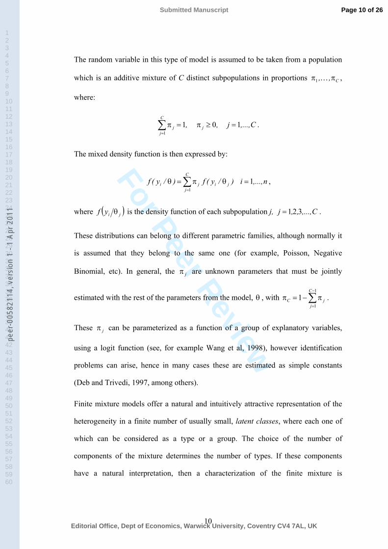
The random variable in this type of model is assumed to be taken from a population

which is an additive mixture of C distinct subpopulations in proportions C,, ππ K1 ,

where:

C,...,j,, j

C

jj 101

1=≥π=π∑

=

.

The mixed density function is then expressed by:

n,...,i)/y(f)/y(fC

jjiji 1

1=θπ=θ ∑

=

,

where ( )jiyf θ is the density function of each subpopulation j, C,...,,,j 321= .

These distributions can belong to different parametric families, although normally it

is assumed that they belong to the same one (for example, Poisson, Negative

Binomial, etc). In general, the jπ are unknown parameters that must be jointly

estimated with the rest of the parameters from the model, θ , with ∑−

=

π−=π1

11

C

jjC .

These jπ can be parameterized as a function of a group of explanatory variables,

using a logit function (see, for example Wang et al, 1998), however identification

problems can arise, hence in many cases these are estimated as simple constants

(Deb and Trivedi, 1997, among others).

Finite mixture models offer a natural and intuitively attractive representation of the

heterogeneity in a finite number of usually small, latent classes, where each one of

which can be considered as a type or a group. The choice of the number of

components of the mixture determines the number of types. If these components

have a natural interpretation, then a characterization of the finite mixture is

Page 10 of 26

Editorial Office, Dept of Economics, Warwick University, Coventry CV4 7AL, UK

Submitted Manuscript

123456789101112131415161718192021222324252627282930313233343536373839404142434445464748495051525354555657585960

peer

-005

8211

4, v

ersi

on 1

- 1

Apr 2

011

For Peer Review

11

interesting, however, this is not essential since the finite mixture can be simply

expressed in a flexible and parsimonious way of modelling the data (Cameron and

Trivedi, 1998).

2.4. Models for a subsample

In some instances, the range of the dependent variable is partially observable or only

one subset of the population is of interest because it represents specific type of

behaviour. For example, only those individuals who have tried at least a certain

number of wine types are considered. This context reveals a truncated sample

towards the left, typically with the truncation at zero, and in our case, only

consumers.

The standard way of gathering this type of behaviour involves the use of Poisson or

truncated Negative Binomial models13. These models coincide with the second part

of the hurdle model discussed earlier. This case is characterized by the assumption

that the behaviour of the dependent variable follows some of these distributions and

that the observed counts are restricted to positive values.

An alternative way to deal with the truncation at zero is by changing the sample

space. This approach is different then the one obtained by the conditional

distribution, and the probability function would be given by:

( ) ...,,y,)!y(

ex/yYP ii

yi

iii

iii

3211

1

=−λ

==−λ−

where now

13 Gurmu (1991), Grogger and Carson (1991), Gurmu and Trivedi (1992), among others, have commented on these models. Recent application in order to look for some evidence of the presence of reputation in the return to tourist destination can be found in Ledesma et al (2005).

Page 11 of 26

Editorial Office, Dept of Economics, Warwick University, Coventry CV4 7AL, UK

Submitted Manuscript

123456789101112131415161718192021222324252627282930313233343536373839404142434445464748495051525354555657585960

peer

-005

8211

4, v

ersi

on 1

- 1

Apr 2

011

For Peer Review

12

[ ][ ] iii

iii

x/yVx/yE

λ=+λ= 1

This distribution is known as the Displaced Poisson (Jonson and Kotz, 1969) and

agrees with the one obtained by Shaw (1988) for the treatment of on-site sampling14.

Although the basis for the truncated distribution and the one obtained from this last

distribution is the same, both are different (Cameron and Trivedi, 1998, p. 331).

Finally, our approach can be extended to the different versions of the Negative

Binomial and the finite mixture model which were presented in previous sections.

The finite mixture model only requires an explanation of how new obtained

distributions for the different classes are going to be considered. The optimization

procedure follows the same steps as in the original.

3. Data and Results

3.1. Data

The data used in this study came from an exhaustive survey regarding wine

consumption in Tenerife which took place during April and May, 2001. The survey

included questions related to residents´ drinking habits and preferences with respect

to wine consumption in general and specifically wine from Tenerife15. The variables

that were used in our analysis include the type of wine consumed, the frequency of

consumption and others of a socioeconomic nature. A description is included in table

1 of the appendix.

We thought it would be important to put together a descriptive analysis of the

number of wine types. This analysis would give us an initial idea about the 14 See Englin and Shonkwiler (1995) for an extension to the Negative Binomial. 15 See Guirao et al (2001) for a detailed description of the survey.

Page 12 of 26

Editorial Office, Dept of Economics, Warwick University, Coventry CV4 7AL, UK

Submitted Manuscript

123456789101112131415161718192021222324252627282930313233343536373839404142434445464748495051525354555657585960

peer

-005

8211

4, v

ersi

on 1

- 1

Apr 2

011

For Peer Review

13

diversification of wine consumption. Some significant results obtained from the

contingency tables between this variable and the frequency of consumption are

discussed. Comparisons with other socioeconomic variables were also performed.

Our first observation is that the majority of individuals who drink wine tend to

choose between one and three different types. Specifically 35.73% of all individuals

tend to drink two different wine types. These two wine type combinations are local

bottled wine with Apellation d´ Origin (A.O.) and imported wine with A.O (29.2%).

The next group includes local table wine and local bottled wine with A.O (25.8%).

When considering those individuals who drink just one type of wine (27.64%), the

most common type was local table wine (35.8%), local bottled wine with A.O.

(33.7%), imported bottled wine with A.O. (16.3%) and self produced local table wine

(12.6%). In addition, 20.67% drink three different types of wines. The most common

combination among this three type group was imported table wine, local bottled wine

with A.O. and imported bottled with A.O., representing 38%.

Table 1. Frequency Distribution: number of wine types

Number of types

Frequency Overall %

% of those that consumer

0 282 24.06 ------ 1 246 20.99 27.64 2 318 27.13 35.73 3 184 15.70 20.67 4 73 6.23 8.20 5 33 2.82 3.71 6 26 2.22 2.92 7 10 0.85 1.13

On the other hand we note from the contingency tables that on average, males

consume 25% more wine types than females. In addition, the average number of

wine types consumed in the first four age categories is practically the same and is

nearly 2, while this average drops to 1.5 for the 60 to 69 age group, before settling

Page 13 of 26

Editorial Office, Dept of Economics, Warwick University, Coventry CV4 7AL, UK

Submitted Manuscript

123456789101112131415161718192021222324252627282930313233343536373839404142434445464748495051525354555657585960

peer

-005

8211

4, v

ersi

on 1

- 1

Apr 2

011

For Peer Review

14

down to 1.0 after age 70. Regarding residence, the southern and metropolitan areas

consume a greater variety of wines, especially among singles and married

individuals. This variety is also greater among professionals, businessmen and civil

servants, while housewives consume a smaller amount of wine types. An increase in

income corresponds to an increase in the variety of wines consumed, although this is

not the case for specific levels of education. For instance, university students and

those individuals with primary school studies are those that consume the greatest

amount of distinct wine types. Regarding consumption frequency we observe that, in

general, as the frequency in wine consumption increases, so does the average number

of wine types consumed. Specifically, those who seldom drink will consume on

average approximately 2 different types of wine, while this figure rises to 2.5 for

those who drink occasionally and 2.8 for those who drink often. Finally the average

number of wine types for those who drink daily is 2.5, although the dispersion of

these with respect to the average number of wine types is the highest of all the

categories.

This relation among the number of wine types and consumption frequency suggests

that frequency, along with other socioeconomic characteristics, can be a determining

factor in the variety of wine types that the individual consumes and is the reason why

it is included as an explanatory variable in the models used in the study.

3.2. Results

Several models have been tested for all individuals and for the sub-sample of

consumers with the aim of analyzing the role of exclusivity in the consumption of

wine. Both cases initially used the Negative Binomial and Poisson models. Two

assumptions are made with respect to the Negative Binomial: one, that the variance

is considered to be proportional to the mean, leading to the NEGBIN I model, and

Page 14 of 26

Editorial Office, Dept of Economics, Warwick University, Coventry CV4 7AL, UK

Submitted Manuscript

123456789101112131415161718192021222324252627282930313233343536373839404142434445464748495051525354555657585960

peer

-005

8211

4, v

ersi

on 1

- 1

Apr 2

011

For Peer Review

15

two, that the variance is defined as a quadratic function of the mean, resulting in the

NEGBIN II model.

Both NEGBIN I and NEGBIN II models reveal that the parameter of dispersion ( )α

is not significant for the sample. This result suggests that the overdispersion present

in the data is not very high (see table 2 in the appendix), which is reasonable given

the relative nearness that exists between the mean and variance of the dependent

variable, 1.8063 and 2.365, respectively.

In order to compare the Poisson model with the negative binomial approximations

we began with the optimal regression-based test proposed by Cameron and Trivedi

(1990) to check for overdispersion or underdispersion in the Poisson model16. This

test is based on the OLS auxilliary regression between ( )[ ] iiiii yyz µ−µ−= 22

and iii )(gw µµ= 2 , where )( ig µ is equal to µ or 2iµ and in the posterior

significance testing of the coefficient. In both cases, this coefficient is practically null

and not significant, indicating scarce presence or absence of overdispersion in the

data. We then use the common LR (likelihood ratios)17 to compare nested models. In

this case no evidence is found to reject the Poisson model against the NEGBIN I and

II models18.

16 ( )

µα+µ=µ=

iii

ii

g)yvar(:H)yvar(:H

1

0

17 )LLnLLn(LR 102 −−= ~ 2qχ , where 0L is the likelihood function for the restricted model and 1L

for the unrestricted model. 18 We previously studied the influence of certain socioeconomic characteristics of the individual on the number of wine types that are being consumed, but without considering the effect of consumption frequency. In this paper the Poisson model was rejected against the two negative binomial estimates using traditional overdispersion tests. This result leads us to consider whether the differences among individuals are not only due to observed heterogeneity but also to unobserved heterogeneity. The unobserved heterogeneity term included in the conditional mean of the negative binomial models can capture the effect of one explanatory variable which has been omitted in the model. The current study includes consumption frequency as the explanatory variable and has not lead to the rejection of the Poisson model against the two negative binomial models. Consequently we can consider that this

Page 15 of 26

Editorial Office, Dept of Economics, Warwick University, Coventry CV4 7AL, UK

Submitted Manuscript

123456789101112131415161718192021222324252627282930313233343536373839404142434445464748495051525354555657585960

peer

-005

8211

4, v

ersi

on 1

- 1

Apr 2

011

For Peer Review

16

A Hurdle Poisson model (HPM) and Finite Mixture Poisson Model (FMPM) (see

table 2 in appendix) are also included with the prior estimates. The Hurdle model

separately models the probability of individual decision to not drink from the one

where he decides to drink a specific number of wine types, while the finite mixture

model considers two components (latent classes) that could initially be interpreted in

relation to the level of exclusivity in the consumption. The dichotomy between these

two groups would be characterized by a mean and variance of the number of wine

types consumed where the first model has a lower value than the second. In our study

the means are, respectively, 1,70 and 2,55, with variances of 0.974 and 6.15.

Similarly the significance of jπ confirms the hypothesis of the two subpopulations,

whose estimated proportions would be 0.847 and 0.153.

Given that the Hurdle Poisson model and the FMPM models are not nested, two

standard choice criteria are used in the comparison, namely the Akaike Information

Criteria (AIC) and the Bayesian Information Criteria (BIC)19 .

Table 2. Model selection (Information Criteria) Criteria/Model Poisson Hurdle

Poisson model

Finite mixture Poisson model

AIC 3547.2 3857.7 3535.4 Total Sample (N=1172) BIC 3704.9 4167.1 3848.3

AIC 2701,9 --- 2665,3 Consumer (N=890) BIC 2878,5 --- 3032,0

Based on the results from the prior table we conclude that the Hurdle Poisson model

should be rejected in favour of the other alternatives, where the Finite Mixture variable has assisted in explaining the individual differences that were initially attributed to unobserved heterogeneity, and specifically, to overdispersión. 19 kLln2AIC +−= ; )Nln(kLln2BIC +−= , where L is the maximum likelihood function, k is the number of parameters that are estimated and N is the number of total sample observations.

Page 16 of 26

Editorial Office, Dept of Economics, Warwick University, Coventry CV4 7AL, UK

Submitted Manuscript

123456789101112131415161718192021222324252627282930313233343536373839404142434445464748495051525354555657585960

peer

-005

8211

4, v

ersi

on 1

- 1

Apr 2

011

For Peer Review

17

Poisson Model is preferred according to the AIC and the Poisson model is favoured

by the BIC.

The nested models allow us to compare using likelihood ratio tests. In this case the

statistic takes on a value of 39.766 which, at the 5% significance level, leads to the

rejection of the Poisson model in favour of the latent class model. Fitted relative

frequencies were calculated for each model, considering the entire sample or only

consumers. For the first case (see table 3) our review reveals that all of the models

under study tend to underestimate the number of zeros and overestimate the number

of ones. Nevertheless good behaviour is observed when counts are greater than or

equal to two. Most of the models adequately capture each one of the counts when

only considering consumers (see table 4). In this situation the finite mixture model

stands out.

Table 3. Actual and fitted distributions: (Relative frequencies for different models)

N=1172

Number of types

Observed Poisson Hurdle Model Finite Mixture

0 0.24 0.16 0.15 0.16 1 0.21 0.30 0.28 0.29 2 0.27 0.27 0.27 0.27 3 0.16 0.16 0.17 0.16 4 0.06 0.07 0.08 0.07 5 0.03 0.03 0.03 0.03 6 0.02 0.01 0.01 0.01 7 0.01 0.00 0.00 0.00

Table 4. Actual and fitted distributions: (Relative frequencies for different models)

N=890

Number of types

Observed Poisson Truncated Poisson Finite Mixture

1 0.28 0.25 0.33 0.29

Page 17 of 26

Editorial Office, Dept of Economics, Warwick University, Coventry CV4 7AL, UK

Submitted Manuscript

123456789101112131415161718192021222324252627282930313233343536373839404142434445464748495051525354555657585960

peer

-005

8211

4, v

ersi

on 1

- 1

Apr 2

011

For Peer Review

18

2 0.36 0.35 0.32 0.36 3 0.21 0.24 0.20 0.22 4 0.08 0.11 0.10 0.09 5 0.03 0.04 0.04 0.03 6 0.03 0.01 0.01 0.01 7 0.01 0.00 0.00 0.00

Age generally influences the number of wine types chosen by the consumer. This

finding is consistent with the Finite Mixture Poisson Model (FMPM). As a result the

number of variety of wine consumed decreases as the individual gets older. This

characteristic is also present in the rest of the models. Other determining factors in

the rest of the models are geographical area and consumption frequency. There is a

wide range among consumption in the southern part of the island, and especially in

the metropolitan area, when compared to the northern part of the island. Nonetheless,

its influence in the finite mixture model is different for both considered classes. For

instance, a significant impact is noted in the southern area for the group of less

exclusive wine drinkers, and for the metropolitan area, it is the most exclusive.

Consumption frequency has a similar effect on both collected classes in the finite

mixture model. This fact can be interpreted as non discriminatory among the

obtained groups.

The income variable does not affect the number of wine types except in the Finite

Mixture Model, although it is noteworthy that this variable is only significant in the

second group of individuals. In this case its effect is negative, displaying greater

exclusivity with income level. Similarly, occupation can also capture the effect of

income, and is also only significant for this part of the model in some categories

(businessmen, professionals and others), where its effect is positive. It is worth

noting the sex variable is not an explanatory factor in any of the models, although it

is interesting that a high correlation exists between the sex variable and the frequency

Page 18 of 26

Editorial Office, Dept of Economics, Warwick University, Coventry CV4 7AL, UK

Submitted Manuscript

123456789101112131415161718192021222324252627282930313233343536373839404142434445464748495051525354555657585960

peer

-005

8211

4, v

ersi

on 1

- 1

Apr 2

011

For Peer Review

19

of consumption, which is significant. Education level, in general, is not significant,

as seen by individuals with university studies who show the greatest variability in our

sample.

With regard to the subsample of wine drinkers, we followed the procedure described

in section 2.4. As observed in Table 2, the obtained results for the choice of models

are the same as those for the complete sample. That is, according to the AIC criteria

the FMPM is preferred, while the BIC criteria points to the Poisson model. The

statistical value of the likelihood ratio test among these nested models is 64.64,

rejecting the Poisson model against the Finite Mixture Model at the 5% significance

level. The proportions for each class are significant for the Finite Mixture Model,

estimated at 0.758 and 0.242, respectively. As we mentioned earlier, this can be an

indication of the presence of two subpopulations that show a different response with

respect to the greater or lesser exclusivity in consumption.

The obtained results are, in some aspects, similar to those obtained for the entire

sample (see table 3 in the appendix). That is, for the standard Poisson model, age,

geographical location and consumption frequency are seen as relevant factors, but

not educational level. The greatest variability is found in the set of individuals with

university studies. This last result is also generated by both groups in the finite

mixture model. Occupation is also not relevant in this model for the least exclusive

group. Note, however, that income has a positive effect in the most exclusives, even

when the negative impact for the first group is obtained. Finally the remaining

factors, which include age, geographical area and consumption frequency, reveal

similar behaviour to that obtained from our entire sample, although in this case the

impact of consumption frequency is lesser for both groups.

Page 19 of 26

Editorial Office, Dept of Economics, Warwick University, Coventry CV4 7AL, UK

Submitted Manuscript

123456789101112131415161718192021222324252627282930313233343536373839404142434445464748495051525354555657585960

peer

-005

8211

4, v

ersi

on 1

- 1

Apr 2

011

For Peer Review

20

4. Conclusion

In this study several approaches regarding the analysis of wine type consumption by

the residents in Tenerife have been presented. Standard approximations (Poisson,

NEGBIN I and NEGBIN II) have been compared with more flexible ones (Hurdle

Poisson Model and the Finite Mixture Poisson Model with two components). These

last two have been proposed as alternatives in the data count context which normally

shows relatively high means and long tails, thus producing greater advantages than

those found in typical parametric versions (Guo and Trivedi, (2002)). In our case, the

count type showed different characteristics than those mentioned, and motivated the

interest in exploring these alternatives from an empirical point of view.

Based on some traditionally used criteria in model selection for count data it can be

concluded that Negative Binomial models are not superior to the Poisson model. A

comparison of the Poisson model with the other two models which do not assume the

same preference structure for consumers and non-consumers (Hurdle Poisson

Models), or those that assume the presence of subpopulations with different response

(Finite Mixture Poisson Model) is carried out. In our study the Poisson model or the

Finite Mixture Poisson Model is chosen according to the criteria utilized.

Nevertheless our results indicate that these models can be, marginally at least, more

appropriate when including this particular type of count. At any rate other semi-

parametric and non-parametric alternatives are open to further research in this area.

A summary of the results obtained from our study regarding the determining factors

based on the level of exclusivity in the consumption of wine shows that, in general,

the age of the individual —where a smaller variety of wine types remain as

individuals age—, the individuals residence —in this case the most exclusive

consumption occurs in the northern part of the island— and drinking frequency are

Page 20 of 26

Editorial Office, Dept of Economics, Warwick University, Coventry CV4 7AL, UK

Submitted Manuscript

123456789101112131415161718192021222324252627282930313233343536373839404142434445464748495051525354555657585960

peer

-005

8211

4, v

ersi

on 1

- 1

Apr 2

011

For Peer Review

21

the most relevant factors. In addition income and education are exceptionally

relevant for certain models. These factors also show behaviour patterns which are

differentiated according to the group of individuals considered in the Finite Mixture

Poisson Model, providing this model perhaps with a more realistic and useful

approach to represent the heterogeneity of the observed phenomena.

5. References

BOSWELL, M.T. and PATIL, G.P. (1970): “Chance Mechanisms Generating the

Negative Binomial Distributions”, in Patil, G.P., Random Counts in Models and

Structures, vol. 1-3, University Park, PA, and London, Pennsylvania State University

Press.

CAMERON, A.C. and TRIVEDI, P.K. (1990): “Regression-based Tests for

overdispersion in the Poisson Model”, Journal of Econometrics, 46, 347-364.

CAMERON, A.C. and TRIVEDI, P.K. (1998): “Regression Analysis of Count

Data”, Cambridge University Press.

CRAGG, J.C. (1971): “Some Statistical Models for Limited Dependent Variables

with Application to the Demand for Durable Goods”, Econometrica, vol. 39, 829-

844.

DEB, P. and TRIVEDI, P.K. (1997): “Demand for Medical Care by the Elderly in

the United States: a Finite Mixture Approach”, Journal of Applied Econometrics, 12,

313-336.

DEB, P. and TRIVEDI, P.K. (2002): “The Structure of Demand for Health Care:

Latent Class versus two-part models”, Journal of Health Economics, 21, 601-625.

ENGLIN, J. and SHONKWILER (1995): “Estimating Social Welfare using Count

Data Models: An Application to Long-run Recreation Demand under Conditions of

Endogenous Stratification and Truncation”, The Review of Economics and Statistics,

77, 104-112.

GOURIEROUX, C., MONFORT, A. and TROGNON, A. (1984a): “Pseudo

Maximum Likelihood Methods: Theory”, Econometrica, 52, pp. 681-700.

Page 21 of 26

Editorial Office, Dept of Economics, Warwick University, Coventry CV4 7AL, UK

Submitted Manuscript

123456789101112131415161718192021222324252627282930313233343536373839404142434445464748495051525354555657585960

peer

-005

8211

4, v

ersi

on 1

- 1

Apr 2

011

For Peer Review

22

GOURIEROUX, C., MONFORT, A. and TROGNON, A. (1984b): “Pseudo

Maximum Likelihood Methods: Applications to Poisson Models”, Econometrica, 52,

pp. 701-720.

GROGGER, J.T. and CARSON, R.T. (1991): “Models for Truncated Counts”,

Journal of Applied Econometrics, 6, 225-238.

GUIRAO, G., CÁCERES, J.J., CANO, V., HERNÁNDEZ, M., LÓPEZ, M.I.,

MARTÍN, F.J. and RODRÍGUEZ, M.C. (2001): El consumo de vino en Tenerife.

Servicio Técnico de Desarrollo Rural y Pesquero, Cabildo Insular de Tenerife.

GUO, J. and TRIVEDI, P. (2002) “Flexible Parametric Models for Long-tailed

Patent Count Distributions”, Oxford Bulletin of Economics and Statistics, 64 (1), pp.

63-82.

GURMU, S. (1991): “Test for Detecting Overdispersion in the Positive Regression

Model”, Journal of Business and Economics Statistics, 9, 215-222.

GURMU, S. and TRIVEDI, P.K. (1992): “Overdispersion Test for Truncated

Poisson Regression Models”, Journal of Econometrics, 54, 347-370.

GURMU, S. and TRIVEDI, P.K. (1996): “Excess of Zeros in Count Models for

Recreational Trips”, Journal of Business and Economics Statistics, 14, 469-477.

HAUSMAN, J.A., HALL, B.H. and GRILICHES, Z. (1984): “Econometric Models

for Count Data with an Application to the Patents-R and D Relationship”,

Econometrica, 52, pp. 909-938.

JOHNSON, N.L. and KOTZ, S. (1969): Discrete Distributions. Boston. Houghton

Mifflin.

LEDESMA, F.J., NAVARRO, M. and PÉREZ J.V. (2005): “Return to tourist

destination. Is it reputation, after all?”, Applied Economics, 37, 2055-2065.

LEISCH, F. (2004): “FlexMix: A General Framework for Finite Mixture Models and

Latent Class Regression in R”, Journal of Statistical Software, 11, 1-18.

LINDSAY, B.G. (1995): “Mixture Models: Theory, Geometry and Applications,

NSF-CBMS Regional Conference Series in Probability and Statistics, vol. 5, IMS-

ASA. Hayward, CA: Institute of Mathematical Statistics.

MULLAHY, J. (1986): “Specification and Testing of Some Modified Count Data

Models”, Journal of Econometrics, 33, 341-365.

MULLAHY, J. (1997): “Heterogeneity, Excess Zeros and the Structure of Count

Data Models”, Journal of Applied Econometrics, 12, pp. 337-350.

Page 22 of 26

Editorial Office, Dept of Economics, Warwick University, Coventry CV4 7AL, UK

Submitted Manuscript

123456789101112131415161718192021222324252627282930313233343536373839404142434445464748495051525354555657585960

peer

-005

8211

4, v

ersi

on 1

- 1

Apr 2

011

For Peer Review

23

NAYGA, R.M. (1996): “Sample selectivity models for away from home

expenditures on wine and beer”, Applied Economics, 28, 1421-1425.

SELVANATHAN, E.A. and SELVANATHAN, S. (2004): “Economic and

demographic factors in Australian alcohol demand”, Applied Economics, 36, 2405-

2417.

SHAW, D. (1988): “On-site Samples Regression”, Journal of Econometrics, 37, 211-

223.

SU S-J.B. and YEN S.T. (2000): “A censored system of cigarette and alcohol

consumption”, Applied Economics, 32, 729-737.

WANG, P., COCKBURN, I.M. and PUTERMAN, M.L. (1998): “Analysis of Patent

Data –A Mixed Poisson Regression Model Approach”, Journal of Business and

Economics Statistics, 16 (1), 27-41.

WINKELMANN, R. and ZIMMERMANN, K.F. (1995): “Recent Development in

Count Data Modelling: Theory and Applications”, Journal of Economics Surveys, 9,

1-24.

YEN, S.T. (1999): “Gaussian versus count-data hurdle models: cigarette

consumption by women in the US”, Applied Economics Letter, 6, 73-76.

Page 23 of 26

Editorial Office, Dept of Economics, Warwick University, Coventry CV4 7AL, UK

Submitted Manuscript

123456789101112131415161718192021222324252627282930313233343536373839404142434445464748495051525354555657585960

peer

-005

8211

4, v

ersi

on 1

- 1

Apr 2

011

For Peer Review

24

Appendix

Table 1. Variables included in the models Frequency of wine consumption FC

Never 0= Seldom 1= Sometimes during a meal 2= Often during a meal 3= During every meal 4=

Sex Dummy variable reflecting gender: male ( )1= , female ( )2=

Age: E1 E2 E3 E4 E5 E6

Dummy variable reflecting age: 18-29 30-39 40-49 50-59 60-69 ≥70

Residence: A1 A2 A3

Dummy variable reflecting residential area: Northern part of island Southern part of island Metropolitan area

Marital Status: SF1 SF2 SF3

Dummy variable reflecting marital status Married Single Widow/Separated

Number of family members MUF

Variable reflecting number of family members in family unit (1,2,3,.....)

Occupation O1 O2 O3 O4 O5 O6 O7

Dummy variable reflecting occupation: Employee Civil Servant Student Housewife Businessman Professional Other

Education ED1 ED2 ED3 ED4

Dummy variable reflecting education: Unfinished studies Primary school student Secondary school student University student

Income I1 I2 I3 I4 I5

Dummy variable reflecting monthly income level (euros) <600 600-1200 1200-1800 1800-2400 >2400

Page 24 of 26

Editorial Office, Dept of Economics, Warwick University, Coventry CV4 7AL, UK

Submitted Manuscript

123456789101112131415161718192021222324252627282930313233343536373839404142434445464748495051525354555657585960

peer

-005

8211

4, v

ersi

on 1

- 1

Apr 2

011

For Peer Review

25

Table 2. Estimation results for entire sample (N=1172)

Hurdle Model Finite Mixture Model (Latent Class)

Poisson NEGBIN I NEGBIN II Logit P- Truncated Class I Class II Variables Coeff. p-value Coeff. p-value Coeff. p-value Coeff. p-value Coeff. p-value Coef. p-value Coef. p-value

Constant -0.947 0.000 -0.946 0.000 -0.947 0.000 1.268 0.005 -0.303 0.184 -0.832 0.000 -2.088 0.020 S2 -0.054 0.301 -0.052 0.361 -0.053 0.342 -0.864 0.000 -0.071 0.252 -0.012 0.859 -0.228 0.284 E1 0.646 0.000 0.646 0.001 0.647 0.000 0.960 0.026 0.502 0.008 0.592 0.002 1.149 0.058 E2 0.586 0.000 0.584 0.001 0.586 0.000 0.747 0.047 0.535 0.002 0.459 0.006 1.389 0.009 E3 0.425 0.001 0.423 0.032 0.426 0.002 0.537 0.125 0.473 0.005 0.234 0.159 1.254 0.007 E4 0.432 0.001 0.429 0.036 0.432 0.003 0.602 0.087 0.500 0.003 0.320 0.054 0.942 0.050 E5 0.166 0.182 0.163 0.248 0.166 0.228 0.369 0.229 0.225 0.177 -0.031 0.854 0.858 0.052 A2 0.129 0.018 0.128 0.027 0.130 0.022 0.021 0.905 0.159 0.016 0.045 0.537 0.431 0.030 A3 0.220 0.000 0.220 0.001 0.220 0.001 0.128 0.511 0.166 0.017 0.233 0.002 0.240 0.340 SF2 0.002 0.979 0.001 0.928 0.002 0.979 -1.138 0.000 0.093 0.290 -0.047 0.606 0.198 0.496 SF3 -0.086 0.292 -0.085 0.348 -0.085 0.336 -0.540 0.028 -0.057 0.567 -0.072 0.481 -0.068 0.818 MUF 0.024 0.130 0.024 0.166 0.024 0.152 0.0005 0.993 0.030 0.108 0.008 0.719 0.078 0.248 O2 -0.104 0.306 -0.105 0.397 -0.104 0.390 0.648 0.211 -0.080 0.510 -0.228 0.071 0.373 0.297 O3 -0.053 0.538 -0.054 0.568 -0.053 0.566 -0.682 0.017 0.052 0.604 -0.138 0.213 0.295 0.432 O4 0.019 0.829 0.017 0.863 0.019 0.842 -0.669 0.012 0.010 0.993 -0.133 0.244 0.706 0.105 O5 -0.0002 0.998 -0.002 0.979 -0.001 0.999 -0.008 0.980 0.097 0.282 -0.161 0.166 0.662 0.016 O6 0.074 0.406 0.072 0.423 0.074 0.400 0.759 0.127 0.111 0.281 -0.089 0.435 0.958 0.015 O7 -0.025 0.781 -0.027 0.778 -0.025 0.788 -0.115 0.705 -0.011 0.923 -0.194 0.095 0.803 0.015 ED2 0.198 0.053 0.199 0.054 0.198 0.051 0.795 0.002 0.078 0.540 0.200 0.160 0.396 0.272 ED3 0.166 0.132 0.166 0.123 0.166 0.114 0.817 0.008 -0.033 0.809 0.065 0.668 0.630 0.113 ED4 0.295 0.013 0.295 0.014 0.295 0.012 1.257 0.000 0.107 0.461 0.174 0.277 0.986 0.035 I2 -0.102 0.228 -0.102 0.239 -0.102 0.231 -0.580 0.024 -0.014 0.891 -0.062 0.601 -0.263 0.371 I3 -0.078 0.376 -0.076 0.418 -0.078 0.402 -0.360 0.200 -0.024 0.820 0.068 0.572 -0.690 0.036 I4 -0.132 0.189 -0.129 0.231 -0.132 0.215 -0.306 0.363 -0.132 0.277 0.118 0.394 -1.297 0.004 I5 -0.118 0.259 -0.116 0.289 -0.118 0.273 0.065 0.863 -0.080 0.525 0.152 0.317 -1.345 0.018 FC 0.409 0.000 0.409 0.000 0.409 0.000 0.153 0.000 0.430 0.000 0.471 0.003 α 0.019 0.683 0.0003 0.999 Ln L -1760.601 -1760.499 -1760.602 -565.248 -1338.331 -1740.718

Page 25 of 26

Editorial Office, Dept of Economics, Warwick University, Coventry CV4 7AL, UK

Submitted Manuscript

123456789101112131415161718192021222324252627282930313233343536373839404142434445464748495051525354555657585960

peer

-005

8211

4, v

ersi

on 1

- 1

Apr 2

011

For Peer Review

26

Table 3. Estimation results for the consumer subsample (N=890)

Finite Mixture Model (Latent Class)

Poisson Class I Class II Variables Coeff. p-value Coeff. p-value Coeff. p-value

Constant -0.924 0.000 -0.969 0.017 -0.903 0.257 S2 -0.086 0.207 -0.052 0.604 -0.129 0.512 E1 0.598 0.004 0.425 0.174 1.371 0.158 E2 0.638 0.001 0.566 0.052 0.889 0.069 E3 0.564 0.002 0.349 0.229 0.874 0.058 E4 0.596 0.001 0.493 0.103 0.762 0.114 E5 0.265 0.144 -0.079 0.786 0.827 0.057 A2 0.193 0.008 -0.085 0.533 0.713 0.000 A3 0.201 0.009 0.287 0.013 0.063 0.796 SF2 0.113 0.242 0.256 0.078 -0.607 0.199 SF3 -0.068 0.534 -0.016 0.922 -0.285 0.345

MUF 0.036 0.130 -0.010 0.759 0.063 0.301 O2 -0.097 0.468 -0.209 0.248 -0.038 0.932 O3 -0.063 0.569 -0.032 0.854 0.252 0.436 O4 0.003 0.978 -0.229 0.219 0.455 0.192 O5 0.119 0.233 -0.167 0.367 0.563 0.084 O6 0.136 0.233 -0.082 0.657 0.352 0.261 O7 -0.014 0.906 -0.237 0.222 0.470 0.194

ED2 0.093 0.502 0.203 0.452 -0.041 0.908 ED3 -0.041 0.784 -0.276 0.341 0.585 0.145 ED4 0.129 0.418 0.044 0.884 0.412 0.353 I2 -0.018 0.874 0.295 0.127 -0.696 0.018 I3 -0.030 0.796 0.415 0.040 -0.866 0.012 I4 -0.161 0.228 0.332 0.155 -0.988 0.012 I5 -0.098 0.480 0.461 0.051 -1.075 0.006 FC 0.185 0.000 0.180 0.000 0.242 0.007 α

Ln L -1337.968 -1305.646

Page 26 of 26

Editorial Office, Dept of Economics, Warwick University, Coventry CV4 7AL, UK

Submitted Manuscript

123456789101112131415161718192021222324252627282930313233343536373839404142434445464748495051525354555657585960

peer

-005

8211

4, v

ersi

on 1

- 1

Apr 2

011