An Analysis of 3D Particle Path Integration Algorithms

JOURNAL OF COMPUTATIONAL PHYSICS 123, 182–195 (1996)ARTICLE NO. 0015

An Analysis of 3D Particle Path Integration Algorithms

D. L. DARMOFAL

Department of Aerospace Engineering, Texas A&M University, College Station, Texas 77843

AND

R. HAIMES

Department of Aeronautics & Astronautics, MIT, Cambridge, Massachusetts 02139

Received October 24, 1994; revised April 28, 1995

the particle velocity data is generated from a numericalsimulation; therefore, the velocity data is only available atSeveral techniques for the numerical integration of particle paths

in steady and unsteady vector (velocity) fields are analyzed. Most some set of discrete times, t n, for n 5 0, 1, 2, ..., N. Theof the analysis applies to unsteady vector fields, however, some particle paths may be calculated in a postprocessing orresults apply to steady vector field integration. Multistep, concurrent (coprocessing) manner. For postprocessing, themultistage, and some hybrid schemes are considered. It is shown

time planes of velocity data are stored at some set numberthat due to initialization errors, many unsteady particle path integra-of iterations typically determined by the amount of disktion schemes are limited to third-order accuracy in time. Multistage

schemes require at least three times more internal data storage storage available. For concurrent processing, the vectorthan multistep schemes of equal order. However, for timesteps field can be updated every iteration of the flow algorithmwithin the stability bounds, multistage schemes are generally more or after some set number of iterations. In either case, theaccurate. A linearized analysis shows that the stability of these

velocity field, u, is only available at some set of discreteintegration algorithms are determined by the eigenvalues of theinstances in time. A consequence of the temporally discretelocal velocity tensor. Thus, the accuracy and stability of the methods

are interpreted with concepts typically used in critical point theory. nature of the velocity data is that the timestep cannot be setThis paper shows how integration schemes can lead to erroneous by the integration algorithm. This is unlike instantaneousclassification of critical points when the timestep is finite and fixed. streamline integration (or steady velocity fields) for whichFor steady velocity fields, we demonstrate that timesteps outside

the timestep can be adaptively varied to account for rapidof the relative stability region can lead to similar integration errors.trajectory changes thereby increasing accuracy. The goalFrom this analysis, guidelines for accurate timestep sizing are sug-

gested for both steady and unsteady flows. In particular, using of this paper is to determine the factors which impact thesimulation data for the unsteady flow around a tapered cylinder, accuracy, efficiency, and memory requirements of particlewe show that accurate particle path integration requires timesteps integration schemes. Although the majority of this paperwhich are at most on the order of the physical timescale of the

focuses on unsteady data integration, some discussion offlow. Q 1996 Academic Press, Inc.

the steady data or streamline integration case is also given.Most related work is concerned with integration of

streamlines in steady flows [1–5]. However, some work onI. INTRODUCTIONunsteady flows has also been done. Darmofal and Haimes

In this paper, we analyze several numerical particle path [6] suggest a particular algorithm for higher order accurateintegration schemes for three-dimensional, unsteady data. particle path calculations. Also, Shirayama [7] has dis-Our discussions are limited to particles which follow the cussed the effects of local truncation errors on a particularlocal vector field (i.e., massless), however, these algorithms class of two-dimensional linear velocity fields. However,can be extended to include forces acting on particles with unlike this work, Shirayama only considered schemes ofmass. The problem which we wish to solve is second-order temporal accuracy.

II. GENERAL CONSIDERATIONSdxdt

5 u(x, t),Since the timestep is generally not controllable by the

particle integration algorithm in unsteady flows, a majorportion of this analysis focuses on quantifying the effectswhere x is the particle location, u is the particle velocity,

and t is the current time. In our particular application, of finite timestep size on the integration accuracy. Also,

1820021-9991/96 $12.00Copyright 1996 by Academic Press, Inc.All rights of reproduction in any form reserved.

3D PARTICLE PATH INTEGRATION ALGORITHMS 183

the particle path integration schemes may be subject to «L 5 ixn11e 2 Sk(xn

e , une )i, (1)

numerical instabilities because of large timesteps. Thus, it«G 5 ix(t) 2 xe(t)i, (2)may be necessary to use an implicit integration scheme

to obtain reasonable (although not necessarily accurate)where xe and ue are the exact particle position and velocity.trajectories for a wide range of flow fields and timestepThe local error is the error made at a single timestep whilecombinations.the global error measures the cumulative effects of errorsIn addition, each time plane of velocity data from numer-from every timestep including any startup procedures. Theical simulations can generally be assumed to require largelocal order of accuracy, p, is defined asamounts of computer memory for storage. Thus, algo-

rithms which need several time planes of velocity data canbe extremely memory intensive either using large amounts «L 5 O(k p11) as k R 0.of internal memory (limiting the size of the problem) orfrequently reading from disk (impacting the computa- The global order of accuracy, r, is defined astional efficiency).

The velocity data is usually only available at discrete«G 5 O(kr) as k R 0 for fixed t 5 Tf .points in space. Thus, the velocity field must be spatially

interpolated from nodal values to the desired spatial loca-Ignoring the startup effects, a scheme with local errortion. However, in this study, we only address the timeO(k p11) gives a global error of order p because O(k p11)accuracy of the particle path integrations and our modellocal errors are made for Tf /k iterations. However, if theproblems have analytic velocity distributions in space. Forlocal error of the startup procedure is O(ki), then thespatially discrete velocity fields, we use a trilinear interpo-global integration error for the scheme is O(kr), wherelation scheme. The reader may consult [6] for details. Simi-r 5 min( p, i) [8]. As we show, the startup error plays anlar interpolation schemes are also described by Shira-important role in the design of particle path integrationyama [7].schemes.Finally, current computational algorithms (used in com-

putational fluid dynamics) are often second-order accurateA. Multistep Schemesin time. If we are using these integration schemes to either

debug solvers or to gain greater insight into the flow physics A generic multistep scheme has the formabout complex geometries, a reasonable constraint on theparticle integration accuracy is that it should not introduceany additional errors. Therefore, we wish to construct par- Os

i50aixn112i 5 k Os

i50biu(xn112i, t n112i),

ticle integration schemes of at least third order so that theerror is smaller than the flow simulation error in the limitas the timestep approaches zero. where s is the total number of steps, a0 5 1, and either

an112s or bn112s is nonzero. For implicit schemes, b0 ? 0and a (typically) nonlinear system of three equations mustIII. ALGORITHM DESCRIPTIONSbe solved at every timestep for the new particle positionxn11. We solve these nonlinear equations using a Newton–The algorithms we consider may be divided intoRaphson technique. Although explicit schemes are simplermultistep and multistage schemes. In either case, we as-to implement than implicit schemes, they are more severelysume that the velocity field is only available at equallylimited by stability restrictions. Coefficients for severalspaced time intervals such that t n 5 nk, where k is themultistep schemes are given in Appendix A.timestep and n is the current iteration index. Almost every

An advantage of multistep schemes is that only onealgorithm we discuss is easily extendible to nonconstantvelocity field, un11, is needed to calculate the new particletimesteps. One typical example of a nonconstant timestepposition, xn11. The previous particle position and velocityalgorithm is given in Appendix B. Furthermore, we assumedata from n to n 1 1 2 s are also needed; however, thesethat the velocity field is defined for any position x.are only point data (i.e., not field data). For a three-dimen-We also use the concepts of local and global accuracy.sional flow, this adds a maximum of 6s additional wordsWe write a generic integration scheme for timestep k asof storage per particle path. The storage of this data isgenerally done in the computer’s internal memory for each

xn11 5 Sk(xn, un), step of the integration; therefore, we refer to this storageas the internal memory usage. If this data were stored ondisk, then the internal memory usage measures the amountwhere Sk may include timeshift operators. The local error,

«L , and the global error, «G , may be defined by of I/O required between disk and the CPU per timestep.

184 DARMOFAL AND HAIMES

For an s-step multistep scheme, the total internal memory a :5 ku(xn, t n),usage is bounded by

b :5 ku(xn 1 a, t n 1 k), (3)

multistep memory # Nf 1 6sNp words xn11 :5 xn 1 As(a 1 b).

where Nf is the number of words necessary to store the The second scheme is the classic 4-stage Runge–Kuttavelocity field and Np is the number of particle trajectories. algorithm which can be writtenAs mentioned previously, the storage requirements for atime plane of data are considerable; thus, Nf @ Np and the a :5 ku(xn, t n),storage for a multistep scheme is approximately the storage

b :5 ku(xn 1 Asa, t n 1 Ask),of a single velocity field.Higher order accurate multistep schemes with s . 1 c :5 ku(xn 1 Asb, t n 1 Ask), (4)

require the generation of startup data for the first s 2 1d :5 ku(xn 1 c, t n 1 k),iterations. Although the local truncation error of an inte-

gration scheme after initialization may be of higher order, xn11 :5 xn 1 Ah(a 1 2b 1 2c 1 d).the presence of startup errors places a limit on the globalaccuracy of many particle path integration schemes. Typi- We denote the algorithms given by Eqs. (3) and (4) ascal approaches for generating this initialization data are RK2 and RK4, respectively. The local truncation error forto use other multistep schemes with smaller timesteps, or RK2 is p 5 2 and for RK4 is p 5 4.to use a multistage scheme. Unfortunately, for this prob- A difficulty with multistage schemes is that they fre-lem, the timesteps are not controllable since they are set quently require velocity data at intermediate times be-by the data generation algorithm. Furthermore, the first tween t n and t n11. For example, RK4 requires velocity dataiteration can only be a 1-step scheme since previous particle at the midpoint (i.e., t n 1 Ask). Since velocity data is onlyposition or velocity data is generally not available. Thus, available at t n, the velocity at intermediate times must bethe local accuracy of the startup scheme is limited by the interpolated from the previous or the current velocityhighest local accuracy achievable using a 1-step scheme. fields. If the interpolant introduces an error which is O(kq)For stable 1-step schemes, Dahlquist’s first stability barrier at the required quadrature point, then the local accuracystates that i # 3. For example, trapezoidal integration of the multistage scheme is p 5 min(q, pe), where pe is the(1-step Adams–Moulton) has a local truncation error local truncation error of the multistage scheme with anwhich is O(k3). Thus, since the global accuracy of a scheme exact interpolant. Therefore, in order to maintain fourth-is min( p, i) and i # 3, the global error for many algorithms order accuracy in the RK4 scheme, the interpolant mustis O(k3). As we discuss in Section B, a similar situation be fourth order (q 5 4) at the half timestep. For equallyarises using multistage schemes for startup such that the spaced time intervals, the desired fourth-order interpo-best global truncation error achievable is again O(k3). lant is

This startup error analysis suggests that the best onecould hope for is an integration scheme which has a third-

un11/2(x) 5 aThun11(x) 1 !a%hun(x)order global error. However, in some circumstances, itshould be possible to improve the startup error by altering 2 aThun11(x) 1 aQhun22(x).the predicted particle positions after additional timeplanesof data become available. One straightforward technique While the velocity is being interpolated in time, the spatialfor doing this would be to simply delay the integration of position remains fixed at the desired x location. For exam-the particle position by a single iteration. Then, the first ple, in the second step of the RK4 scheme, the desiredupdate of the particle position would have three data location is x 5 xn 1 Asa. The resulting four-stage Runge–planes available and a higher order accurate, 3-step scheme Kutta scheme with the fourth order interpolant is denotedcould be used increasing the startup accuracy to i 5 4. as RK44. This scheme can be thought of as a hybrid be-Whether or not this integration delay is acceptable will tween a multistage and a multistep scheme since the basedepend on the particular application. scheme is multistage while the interpolant is essentially a

multistep approximation.B. Multistage Schemes To illustrate the loss of accuracy which occurs when a

lower order accurate interpolant is used in conjunctionMultistage schemes are difficult to write in a single, uni-with the RK4 scheme, we consider a linear interpolantfied form, therefore, we concentrate on two specific exam-between t n and t n11,ples from the Runge–Kutta family of multistage schemes

[9]. First, the 2-stage Runge–Kutta algorithm often calledthe Heun method is written un11/2(x) 5 Asun11(x) 1 Asun(x).


The resulting scheme would have a local accuracy of p 5d :5 2ku(xn 1 c, t n 1 2k),

min(2, 4) 5 2. We denote this fourstage scheme with linearinterpolation as RK42. A simple example which shows the xn12 :5 xn 1 Ah(a 1 2b 1 2c 1 d),loss of accuracy of the RK42 scheme is a velocity fieldwhich only depends on time u 5 u(t). Thus, using a linear which we denote the RK4 23 scheme. The particle positioninterpolant with Eq. (4) and assuming u 5 u(t), the is updated only every other timestep in this scheme. Thefourstage scheme is identical to the two-stage method given RK4 23 scheme does not require any interpolant for thein Eq. (3). Therefore, the RK42 scheme is not fourth order intermediate values because they are located at t n11. Also,but rather it is second order. the scheme does not require any startup information and

The internal memory usage of the higher order, hybrid has a global accuracy which is fourth order, O((2k)4), spe-schemes can be significant because q planes of velocity cifically. In comparison to the RK4 scheme, the memoryfield data are needed to construct the interpolant. The usage is also reduced to 3Nf 1 3Np words which is stillentire field of velocity data must be stored because the about three times a multistep scheme memory usage. How-particle position at the intermediate times is unknown. ever, the RK4 23 scheme has two significant disadvan-Thus, it must be possible to calculate the velocity at any tages. First, the stability limit is halved because of thespatial location. The total internal memory usage for a timestep doubling. We discuss this further in Section IV.three-dimensional hybrid multistage scheme is Second, unlike the previously discussed multistep and

multistage schemes, the RK4 23 scheme is not easily ex-tendible to nonconstant timesteps.multistage memory # qNf 1 3Np words.

Although spatial interpolation and accuracy is not ad-dressed in this paper, an additional complication arisesThus, the ratio of multistage to multistep internal memorywhen using multistage schemes when the underlying gridusage ischanges in time. In this case, the previous grid information(i.e., spatial locations of nodes) is also necessary to interpo-multistage memory

multistep memory5

qNf 1 3Np

Nf 1 6sNpP q. late the velocity field at the desired intermediate time.

Thus, the memory requirements double assuming the gridinformation storage is the same order as the velocity field

Since the storage for the field information is generally storage. Also, if the particular spatial location does notmuch greater than the number of particles, this ratio is exist at a previous time needed to form the time interpolantapproximately q. Therefore, on memory considerations (e.g., the location was previously in the interior of a movingalone, higher order multistep schemes are much more effi- object), the time interpolant cannot be constructed andcient than the higher order multistage schemes. the particle integration aborts. With a multistep algorithm,

Unlike the classic RK4 scheme, the hybrid RK44 scheme the particle integration aborts only when the particle actu-must now have special startup procedures for the initial ally encounters a domain boundary at the current time.interpolant. At the first step of the algorithm, only two Although the RK4 schemes we have considered are ex-velocity fields are generally available, u0 and u1. If previous plicit, they still require four velocity evaluations per time-velocity fields are available (say, for example, the particle step. In our visualization applications for unstructuredtrace initiation is delayed for q iterations of the flow solver), grids [5], the process of finding a spatial location withinthen it is possible to construct a higher order interpolant the grid and then constructing the velocity interpolant iseven at the first timestep. However, in the situation where typically the most significant portion of the computationalthe particle is released without any delay, the interpolant effort per timestep. By comparison, the implicit multistepin the first step can be only a linear interpolant which has schemes, such as BD4, require a velocity evaluation fora q 5 2 error. Therefore, we are faced with the same every subiteration of the Newton–Raphson solution pro-accuracy barrier as in the multistep schemes. Namely, the cess. Our experience with the BD4 scheme has shown thatstartup scheme has a local error which is at best O(k3), so typically 2–4 subiterations are required; thus, the numberthe global error is at best O(k3). of velocity evaluations for BD4 is usually less than or equal

A final possible higher order multistage scheme is the to the number of velocity evaluations for the RK4 schemes.RK4 scheme applied to timesteps of value 2k. This scheme As a result, no significant difference in computational ef-is written fort exists between the RK4 and BD4 schemes.

a :5 2ku(xn, t n), IV. ANALYSIS OF LINEARIZED PROBLEM

b :5 2ku(xn 1 Asa, t n 1 k),In this section, we consider a linearized velocity field,

such thatc :5 2ku(xn 1 Asb, t n 1 k),


x̃n11i 5 g(li k)x̃n

i ,

where g(li k) is the scheme dependent amplification orgrowth factor. Higher order multistep schemes generateparasitic roots, where more than one growth factor existsfor a given li k. These parasitic solutions are a result ofthe numerical approximation and do not track the equationbeing solved. When multiple growth factors exist, we limitourselves to the growth factor with the largest magnitude,since as time goes to infinity, this root dominates all others.For the exact answer, the amplification factor, ge(li k), is

ge(li k) 5 elik.

FIG. 1. Flow classifications in eigenvalue plane, l1,2,3, 5 eig(u/x).In the following, we investigate the relative stability and

accuracy of: second-order, single-stage Adams–Moultonor trapezoidal integration (TRAP); fourth-order back-

u(x, t) 5 u(0, 0) 1ut

t 1ux

x. wards differentiation (BD4); fourth-order Adams–Bashforth (AB4); and RK4.

If we travel with velocity, u(0, 0) 1 (u/t)t, the nature ofA. Relative Stabilitythe flow around the current location is determined by the

velocity tensor, u/x. In particular, the eigenvalues of the The absolute stability region of a scheme is the area invelocity tensor, l1,2,3 , are the fundamental quantities which the li k plane for which ug(li k)u , 1. For the exact answer,determine the qualitative features of the flow pattern. The the left-half plane is stable while the right-half plane isstudy of the eigenvalues of the velocity tensor is a well- unstable. Although many numerical algorithms are con-researched topic in the classification of critical point flow cerned only with absolute stability, relative stability is of[10–12]. The various possible flow patterns and the corre- primary interest for particle path integrators. For example,sponding eigenvalue-based flow classifications are summa- if the physical mode of a system were (un)stable, therized in Fig. 1. resulting mode of the numerical scheme should also be

The velocity tensor eigenvalues also play a significant (un)stable.role in determining the stability and accuracy of the numer- In Fig. 2, the magnitude of the growth factors for eachical integration schemes. For the linear problem, a second- of these schemes is plotted. The stability boundary (fromorder scheme can integrate exactly the particular solution which the relative stability boundary can be inferred) isdue to the u(0, 0) 1 (u/t)t terms. Since all of the schemes denoted by the circles. TRAP is the only scheme consid-we analyze are at least second order, we do not consider ered for which the numerical stability boundary and thethe nonhomogeneous term. The integration of the homo- exact stability boundary are the same. For example, thegeneous portion due to u/x produces errors and it is stability boundary of RK4 does not include all of the left-these errors which we quantify further. Neglecting the non- half plane. Thus, for the RK4 scheme, some modes whichhomogeneous terms, the linearized problem becomes should be damped actually grow in time. As an example,

we use the RK4 scheme to integrate the two-dimensionalmodel flow from Murman and Powell [1]:dx

dt5

ux

x. (5)

u 5 ax 2 by, (7)This coupled system of three equations can be decoupled

v 5 ay 1 bx. (8)into the respective eigenmodes,

The exact particle paths are then given bydx̃i

dt5 li x̃i , (6)

xe(t) 5 exp(at)[x0 cos bt 2 y0 sin bt],

ye(t) 5 exp(at)[x0 sin bt 1 y0 cos bt].where x̃i is the amplitude of an eigenmode. The numericalscheme is applied to Eq. (5); however, it is straightforwardto show that each eigenmode behaves as if the scheme were For this example, we set a 5 21, b 5 3 which gives an

inward spiraling flow. For these coefficients, the stabilityapplied to Eq. (6) directly. We write the update scheme as


FIG. 2. Magnitude of growth factor in li k plane. u gu , 1, solid line; ugu 5 1, circles; ugu . 1, dashed line.

boundary of the RK4 scheme is exceeded when k $ 0.89. deceleration. Although this cannot be seen from the plot,the region of instability for BD4 is actually bounded and,In Fig. 3, the exact particle path is compared with the RK4

paths for k 5 0.88 and k 5 0.90 for a starting location of for large values of uli ku in the right-half plane, the unstablephysical modes are actually damped by the numerical algo-(x0 , y0) 5 (1, 0). Using the unstable timestep, k 5 0.90,

clearly gives an outward spiraling path; however, the stable rithm. AB4 has significant stability constraints as is ex-pected because of its explicit nature. By contrast, the ex-timestep, k 5 0.88 gives an inward spiraling path as one

would expect from the exact path. This type of behavior plicit multistage scheme, RK4, has a much larger relativestability region.also can affect the integration of steady velocity fields (see

Section A).B. Accuracy

The BD4 scheme is stable along the entire negative realaxis (only a portion of which is visible in Fig. 2); this Although a scheme may be operating within its relative

stability region, the accuracy of the algorithm is still un-can be extremely advantageous for flows exhibiting rapid

FIG. 3. Comparison of exact particle path with numerical paths for stable and unstable timesteps, RK4 algorithm. Initial particle location (x0 ,y0 ) 5 (1, 0).


FIG. 4. Contour plots of 2log E in li k plane.

known. The truncation error can give some accuracy infor- V. NUMERICAL STUDY OF ALGORITHM ACCURACYmation but is only valid in the limit k R 0. Instead, we

In this section, we consider the performance of severalassess accuracy using the growth factor error, E, which weparticle path integration schemes for some simple modeldefine asproblems. The schemes, a short description, and theirglobal accuracy are listed in Table I. The startup schemesfor the AB4 algorithm are the lower order AB algorithms

E(li k) 5 Ug(li k) 2 ge(li k)ge(li k) U. while the initialization method for BD4 first uses TRAP,

followed by BD2 and BD3. We use TRAP instead of BD1in the first step of the BD4 algorithm because of the better

The growth factor error includes the effects of both ampli- accuracy at no extra cost. We compare the numerical andfication and phase error. Figure 4 contains plots of log E exact particle positions by defining the average global errorin the li k complex plane for all four schemes. For uli ku , to be0.5, the second order nature of the TRAP scheme is evidentin comparison to the other schemes all of which are fourth

« 5 (k/Tf ) OTf /k

i51ixi 2 xe(t i)i,order. However, for large values of uli ku, TRAP is actually

competitive with BD4 and AB4.The stability limitations of the AB4 scheme can be recalling that Tf is the final time. « is simply an average of

clearly seen by the significant decrease in accuracy in the the global error, «G (see Eq. (2)), at every timestep.left-half plane. Another interesting aspect of these plots The first model problem is a steady swirling flow withis the poor accuracy of the BD4 scheme for Real(li k) , an axial velocity gradient. Specifically, the velocity field20.45. Although BD4 is stable along the entire negative and eigenvalues are:real axis, its accuracy is quite poor. However, since thesemodes decay quite rapidly, this should not significantly u 5 ar ydegrade the overall accuracy of the method. Of all schemes, v 5 2ar x ⇒ l1,2 5 6iarRK4 appears to offer the best accuracy over a range offinite li k. w 5 azz l3 5 az .


TABLE I

Global Error (r) and Summaries of Schemes Used in Numerical Studies

r Scheme Description

2 TRAP Trapezoidal integration3 BD4 Fourth-order backwards differentiation, O(k3) startup2 AB4 Fourth-order Adams–Bashforth, O(k2) startup2 RK2 Second-order Runge–Kutta2 RK42 Fourth-order Runge–Kutta, O(k2) interpolant3 RK44 Fourth-order Runge–Kutta, O(k4) interpolant, O(k3) startup4 RK4 23 Fourth-order Runge–Kutta, double timestep

For these results, ar 5 1.0 and az 5 20.1; thus, the swirling This model mimics a flow with large unsteadiness but rela-tively small spatial gradients. The exact answer for thiscomponent of the flow dominates the stability and accuracy

of the results. Starting with an initial condition of x0 5 flow is simply, z 5 z0 1 t a. Thus, schemes with a11 z/t a11

as the lowest order derivative in the global error can exactlyy0 5 z0 5 1, we ran each simulation until Tf 5 100 for avariety of timestep sizes; the results appear in Fig. 5 and integrate this velocity field. Table III shows the results for

Tf 5 1, k 5 0.02, and a 5 2 and 3. Schemes which use thethe asymptotic error slopes are tabulated in Table II. Theslopes of TRAP, AB4, and RK2 are clearly second order exact particle positions for startup are included in the table

for comparison. For the a 5 2 case, only AB4 is inaccurate;while RK4, RK44, and RK4 23 are fourth order. The BD4algorithm is nearly third-order accurate with a slope of this is a result of the startup error from the initial AB1

iteration. When the exact startup positions are used to2.93. Thus, the impact of the startup error for AB4 andBD4 can be clearly seen. Also, for larger timesteps, the generate the necessary initial data, (see the AB4 es results

in Table III), this startup error is eliminated and the fourth-instability of the AB4 scheme is evident in the large error.We next consider a simple time-dependent flow with no order Adams–Bashforth scheme performs well for a 5 2.

For a 5 3, startup errors are present in the AB4, BD4,spatial velocity variations.and RK44 results. The large error in the RK42 results isfrom the use of a second-order interpolant. As discussedu 5 0in Section III.B, this lowers the RK42 scheme to onlyv 5 0 ⇒ l1,2,3 5 0second-order accuracy. In fact, RK42 is equivalent to theRK2 and TRAP schemes when no spatial variations exist.w 5 at a21

FIG. 5. Results from Model #1: ar 5 1, az 5 20.1, Tf 5 100, x0 5 y0 5 z0 5 1. Note. Results for RK42 and RK44 scheme are identical forsteady vector fields.


TABLE IIIThe loss of accuracy and equivalence of RK2, RK42, andTRAP are clearly observed from the data of Table III. Results from Model #2Note, these three schemes do not require any special

log « astartup procedures. From this model’s results, we concludethat lower order startup and interpolation can significantly

Scheme 2 3degrade the accuracy of the particle path integration espe-cially for flows with large unsteadiness. TRAP 215.80846 23.99140

BD4 214.91478 24.67769The final model flow has a large, unsteady axial gradientBD4 es 214.66056 214.85560of the axial velocity and steady velocity fields in the otherAB4 23.39794 24.55909directions. Specifically,AB4 es 216.20640 215.77275RK2 215.80846 23.99140

u 5 2x l1 5 21 RK42 215.80846 23.99140RK44 215.80846 25.39794

v 5 20.1y ⇒ l2 5 20.1 RK44 es 216.20640 215.77275RK4 23 2Infinity 215.57438w 5 a0zeatt l3 5 a0eatt.

Note. Tf 5 1, k 5 0.02, x0 5 y0 5 z0 5 1; es 5 exact startup.As a0 R y, the flow has very large axial gradients initiallywhich die away exponentially with at t for at , 0. The

RK44 results, the predicted order of accuracy is attainedTRAP and BD4 algorithms are well-suited for this typein this model; the RK44 scheme still attains fourth-orderof flow field because of their excellent stability propertiesaccuracy, contrary to the third-order startup error presentalong the negative real axis. Although neither BD4 orin the scheme.TRAP accurately represent the large axial velocity gradi-

ent, they are stable and this allows the timestep to be setVI. TIMESTEP LIMITSfor accurately capturing the moderate flow variations in

other directions. The results for a0 5 220 and at 5 20.1 From the previous analysis, we have found that the ei-appear in Fig. 6 and Table II. Since we are more concerned genvalues of the velocity tensor have a major impact onwith the accuracy of the x and y directions, the abscissa is the accuracy of particle path integrations. In this section,labeled by ax k. The TRAP and BD4 schemes perform this analysis is used to properly select the timestep for bothwell over a wide range of timesteps while the other schemes steady and unsteady velocity fields. In either the steady orsuffer at moderate timesteps because of instability from unsteady case, the timestep could be constrained to satisfythe large axial gradients. Thus, TRAP and BD4 may be E(li k) , « where « is some predetermined allowable error.more robust than the explicit multistage schemes and may In the worst case, the cumulative error would be N E,be desirable for some flows, especially flows with large where N is the number of integration steps. This assumesflow variations in one direction while relatively moderate the local growth factor error does not cancel previous localvariations in the other directions. Note, the asymptotic errors. In the following, we use « 5 1023. In our applicationserror slopes from Table II show that the TRAP, AB4, and of the previous integration schemes, we have found « 5RK2 schemes are second order, BD4 is third order, and 1023 generally gives accurate results. Figure 4 can be usedRK44 and RK4 23 are fourth order. Thus, except for the to guide the selection of an appropriate timestep given an

estimate for the velocity tensor eigenvalues and a particularintegration scheme. Then, the timestep restriction can be

TABLE II satisfied byAsymptotic Slopes of Error from Models #1 and #3 Results in

Figs. 5 and 6 kmax 5uli ku«ulmax u

, (9)

log « vs. log ak slopewhere lmax is the largest magnitude eigenvalue and uli ku«

Scheme Model #1 Model #3 is the smallest magnitude of li k which guarantees thatE(li k) , « when uli ku , uli ku« . The procedure to enforceTRAP 2.00 2.00these timestep limits for steady and unsteady flows is de-BD4 2.93 2.94

AB4 2.00 1.95 scribed below.RK2 2.00 2.03RK44 4.00 4.04 A. Steady DataRK4 23 4.00 4.07

For steady flows, timesteps may be adaptively sized toNote. Slopes calculated from final two data points of each line. account for local flow variations. The goal is to use a time-


FIG. 6. Results from Model #3: a0 5 220, at 5 20.1, Tf 5 20, x0 5 y0 5 z0 5 1.

step which is as large as possible while maintaining accept- the magnitudes of the elements of u. This estimate canbe derived using the matrix norm to bound the largestable accuracy. The timestep from Eq. (9) can lead to time-

step limits which are distinctly different than those eigenvalue and then specifically employing the 1-norm andinfinity-norm to arrive at the particular expression. In prac-previously suggested by other authors [1, 3, 7]. These au-

thors suggested setting the timestep such that the particle tice, we employ a timestep limit which is a blend of bothlimits,does not travel more than a given fraction of the length

of a cell in an integration step,

kmax 5 min Shluuu

, uli ku«ul̃max u

D . (11)kmax 5

hluuu

, (10)

The cell fraction timestep limit is used to avoid errors whenwhere l is a measure of the local cell size, h is the allowablethe flow may have significant variations in the velocityfraction of the cell size which a particle may travel in atensor from cell-to-cell.single step, and uuu is the magnitude of the local velocity.

Problems associated with timestep limits based on Eq.However, this timestep limit could result in significant dif-(10) have been observed by Murman and Powell [1] forficulties in a region where the flow speed is near zero andtrajectory integrations of vortical flows using the modelthe cell size is finite. In this case, the timestep can growvelocity field in Eqs. (7) and (8), as well as computedunbounded, resulting in significant errors unless the eigen-conical flow vortex solutions. In their case, trajectory limitvalues of the velocity tensor are small.cycles occurred as the particle approached the center ofFrom a practical point of view, the timestep limit of Eq.the vortex; this phenomenon is a result of the timestep(9) requires the computation of the eigenvalues of the localincreasing as the particle neared the core axis and uuu Rvelocity tensor. Since this is expensive even for a 3 3 30. The limit cycle occurs at a radial location where thematrix, a more efficient technique would be to use antimestep is no longer in the relative stability region ofestimate for the magnitude of the largest possible eigen-the integrator. We illustrate this using a forward Eulervalue. One possible estimate for the largest eigenvalue isintegration scheme (i.e., AB1) which is also the integratorl̃max , defined asused by Murman and Powell. For a forward Euler scheme,the constraint that E , 0.001 requires that uli ku« 5 0.04ul̃max u 5 min[max(uux u, uuy u, uuz u),approximately. To duplicate the previous results of Mur-

max(u=uu, u=vu, u=w u)] $ ulmax u, man and Powell, a grid of square cells with length l 5 0.08is used, the velocity constants are a 5 2As and b 5 3, andthe cell fraction is h 5 1.0. Then, a particle path is inte-where ux is the x derivative of the velocity vector, = is the

gradient operator, and the vector norm uuu is the sum of grated starting from (x, y) 5 (1, 0) using a forward Euler


FIG. 7. Particle trajectories for steady flows using forward Euler integrator and different timestep limits.

integrator and the timesteps based on Eqs. (10) and (11).kmax 5 min Shl

uuu, uli ku«ul̃max u

, hutuD , (12)The results are shown in Fig. 7. The limit cycle previouslynoted by Murman and Powell is evident when the timestepis set by Eq. (10); however, the problem is eliminated by where tu is the approximate timescale of the flow unsteadi-the use of Eq. (11). Murman and Powell eliminated this ness and hu is some fraction used to ensure the flow un-limit cycle by increasing the accuracy of their integrator steadiness is accurately integrated. To satisfy the timestepand decreasing h. However, this strategy does not guaran- limit of Eq. (12), the user must have some knowledge oftee the problem is eliminated for all flowfields and grids. the largest eigenvalue and the timescales expected in theA better strategy which corrects the central difficulty is to flow. To guarantee that all possible particle paths are accu-use a timestep based on the local eigenvalues of the velocity rately calculated, this constraint must be satisfied at alltensor. As can be seen from Fig. 7, acceptable answers can spatial locations, or, at a minimum, the constraint shouldbe obtained when the correct timestep limit is used, even be satisfied at all spatial locations for which the particlewith a low accuracy integrator. paths are desired.

To better understand the practical implications of Eq.B. Unsteady Data

(12), we calculated the eigenvalue spectrum for the taperedcylinder calculation of Jespersen and Levit [13] at NASAFor unsteady flows, the timestep cannot be varied by

the particle integration algorithm and is set by the timestep Ames. This computation features unsteady vortex shed-ding off of a tapered cylinder at a Reynolds number ofbetween available planes of velocity data. Before visualiza-

tion, the timestep is generally sized by the user. If the 150 based on midspan cylinder radius, R. The convectivetimescale of the flow is defined as t 5 R/Uy , and at thisuser is coprocessing, the timestep can be set equal to the

timestep of the flow algorithm. If the user is postprocessing, Reynolds number, we expect the timescale of the unsteadi-ness to be the same order as t. Thus, based solely on thethe timestep must then be set not only by the desired

accuracy level but also by the amount of available external expected unsteadiness, the maximum timestep should beon the order of hut. The eigenvalues are from the velocitymemory. In general, the particle timestep, k, is an integer

multiple, m, of the flow solver timestep, Dt, data at t 5 1200t. To calculate the eigenvalues, the hexahe-dral computational cells were divided into six tetrahedra.Tetrahedral cells result in a unique linear interpolationk 5 mDt.and therefore constant gradients and eigenvalues withineach tetrahedron. The outer envelope for the velocity ten-Minimizing the total external memory requires the user to

maximize m while preserving accuracy. sor eigenvalue spectrum is shown in Fig. 8. The imaginaryportion of the envelope extends to approximately 60.8The timestep limit of Eq. (11) is based solely on spatial

variations of the flow; however, for unsteady flows, the and the real portion extends from 20.53 to 0.45. Note, theeigenvalue contour spikes along the real axis correspondtemporal variations should also be considered when de-

termining the appropriate timestep size. This suggests the to the one purely real eigenvalue which always exists. Inorder for the eigenvalue spectrum to be contained withinfollowing addition to the timestep limit,


FIG. 8. Outer envelope of velocity tensor eigenvalues for Jespersen and Levit [13] tapered cylinder calculation.

the E 5 0.001 contour in Fig. 4, RK4 and BD4 require constraint must be used. However, regardless of whetherthe weak or strong timestep constraint is used, we concludekmax 5 0.7t and 0.3t, respectively. A weaker constraint

would require that the eigenvalue timestep limit be satis- that accurate particle path integrations for this data setrequire timesteps at most on the order of the physicalfied only over a significant portion of the flow. The applica-

bility of this weaker accuracy constraint can be judged timescale of the flow.Finally, the calculation of accurate particle paths in ausing Fig. 9 which is a plot of the distribution of the eigen-

value magnitude. Over 90% of the eigenvalues for this postprocessing mode could produce significant demandson the external memory requirements if the simulationcalculation have magnitude below 0.2. If we enforce the

weak constraint by containing all eigenvalues with magni- length lasts several physical timescales. In the Jespersenand Levit data set, the computational timestep was Dt 5tude below 0.2 in the E 5 0.001 contour, the approximate

timestep requirements for RK4 and BD4 are kmax 5 2.8t 0.1t. Thus, strict enforcement of the accuracy constraintrequires m 5 7 and 3 for RK4 and BD4 while weak enforce-and 1.2t. Although only a small fraction of the eigenvalues

are near magnitude 1.0, if particle paths will be integrated ment requires m 5 28 and 12 for the same schemes. Thus,the RK4 scheme requires less external memory than thethrough these regions, then the previous strong timestepBD4. For the strict constraint, the number of data planesis on the order of the number of integration steps of theflow solver. The weak constraint allows an order of magni-tude decrease in the external memory requirements. If theunsteadiness timescale, tu , is large, such that kmax is beingrestricted by the eigenvalue accuracy constraint, some ofthe external memory demands could be lessened by con-structing an interpolant between data planes. Then, usingthe interpolant to reconstruct the velocity data at thesmaller timestep required by the eigenvalue constraint, itshould be possible to maintain accuracy as well as to de-crease the external memory demands. A different ap-proach to alleviate the external memory demands of post-processing unsteady data sets would be to calculate and/or visualize the particle paths in a coprocessing mode [14].

VII. CONCLUSIONS

We have analyzed a variety of particle path integrationFIG. 9. Fraction of eigenvalues, f(lt), with magnitude less than ultufor Jespersen and Levit [13] tapered cylinder calculation. schemes suitable for use with unsteady velocity fields. In


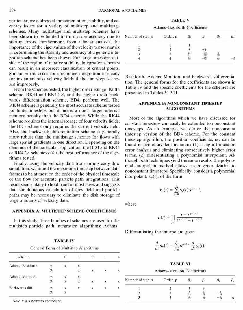
TABLE Vparticular, we addressed implementation, stability, and ac-curacy issues for a variety of multistep and multistage Adams–Bashforth Coefficientsschemes. Many multistage and multistep schemes have

Number of step, s Order, p b1 b2 b3 b4been shown to be limited to third-order accuracy due tostartup errors. Furthermore, from a linear analysis, the

1 1 1importance of the eigenvalues of the velocity tensor matrix2 2 Ds 2As

in determining the stability and accuracy of a generic inte- 3 3 SaDs 2AaHs aTs

gration scheme has been shown. For large timesteps out- 4 4 GsGf 2GsLf DsJf 2sOf

side of the region of relative stability, integration schemescan result in an incorrect classification of critical points.Similar errors occur for streamline integration in steady

Bashforth, Adams–Moulton, and backwards differentia-(or instantaneous) velocity fields if the timestep is cho-tion. The general forms for the coefficients are shown insen improperly.Table IV and the specific coefficients for the schemes areFrom the schemes tested, the higher order Runge–Kuttapresented in Tables V–VII.scheme, RK44 and RK4 23, and the higher order back-

wards differentiation scheme, BD4, perform well. TheAPPENDIX B: NONCONSTANT TIMESTEPRK44 scheme is generally the most accurate scheme tested

ALGORITHMSfor finite timesteps but it incurs a much larger internalmemory penalty than the BD4 scheme. While the RK44 Most of the algorithms which we have discussed forscheme requires the internal storage of four velocity fields, constant timesteps can easily be extended to nonconstantthe BD4 scheme only requires the current velocity field. timesteps. As an example, we derive the nonconstantAlso, the backwards differentiation scheme is generally timestep version of the BD4 scheme. For the constantmore robust than the multistage schemes for flows with timestep algorithm, the position coefficients, ai , can belarge spatial gradients in one direction. Depending on the found in two equivalent manners: (1) using a truncationdemands of the particular application, the BD4 and RK44 error analysis and eliminating consecutively higher erroror RK4 23 schemes offer the best peformance of the algo- terms, (2) differentiating a polynomial interpolant. Al-rithms tested. though both techniques yield the same results, the polyno-

Finally, using the velocity data from an unsteady flow mial interpolant method allows easier generalization tosimulation, we found the maximum timestep between data nonconstant timesteps. Specifically, consider a polynomialframes to be at most on the order of the physical timescale interpolant, xp(t), of the formof the flow for accurate particle path integrations. Thisresult seems likely to hold true for most flows and suggeststhat simultaneous calculation of flow field and particle xp(t) 5 O4

i50ci(t) xn112i,

paths may be necessary to eliminate the disk storage oflarge amounts of velocity data.

where

APPENDIX A: MULTISTEP SCHEME COEFFICIENTS

ci(t) 5 pj?i

t 2 t n112j

t n112i 2 t n112j.

In this study, three families of schemes are used for themultistep particle path integration algorithms: Adams–

Differentiating the interpolant gives

TABLE IV ddt

xp(t) 5 O4i50

xn112i ddt

ci(t).General Form of Multistep Algorithms

Scheme 0 1 2 3 4

TABLE VIAdams–Bashforth ai x xbi x x x x Adams–Moulton Coefficients

Adams–Moulton ai x xNumber of step, s Order, p b0 b1 b2 b3bi x x x x x

Backwards diff. ai x x x x x 1 2 As Asbi x 2 3 aTs aIs 2aQs

3 4 sOf AsLf 2sTf sQfNote. x is a nonzero coefficient.


TABLE VII REFERENCES

Backwards Differentiation Coefficients1. E. M. Murman and K. G. Powell, AIAA J. 27(7), 982 (1989).

2. D. Modiano, M. Giles, and E. Murman, AIAA Paper 89-0138,Number of step, s Order, p b0 a1 a2 a3 a41989 (unpublished).

3. T. Strid and A. Rizzi, Development and Use of Some Flow Visualiza-1 1 1 212 2 Sd 2Fd Ad tion Algorithms. VKI Lecture Series on Computer Graphics and3 3 aYa 2AaKa aOa 2aWa Flow Visualization in CFD, 1989.4 4 AsSg 2FsKg DsHg 2AsHg sEg 4. G. Volpe, AIAA Paper 89-0140, 1989 (unpublished).

5. M. Giles and R. Haimes, Comput. Systems Eng. 1(1), 51 (1990).

6. D. Darmofal and R. Haimes, AIAA Paper 92-0074, 1992 (unpub-lished).

Finally, since we are interested in calculating the time7. S. Shirayama, J. Comput. Phys. 106, 30 (1993).

derivative of the particle position at t n11, the position coef-8. L. N. Trefethen, ‘‘Finite Difference and Spectral Methods,’’ MITficients, ai , can be found by simply equating the coefficients Course Notes, 1989 (unpublished).

for (d/dt)xp at t n11. This gives9. J. C. Butcher, ‘‘The Numerical Analysis of Ordinary Differential

Equations’’ (Wiley, New York, 1987).

10. A. E. Perry and M. S. Chong, Annu. Rev. Fluid Mech. 19, 125ai 5dci

dt Utn11

. (1987).

11. M. S. Chong, A. E. Perry, and B. J. Cantwell, Phys. Fluids A 2(5),765 (1990).

ACKNOWLEDGMENTS12. H. Vollmers, H.-P. Kreplin, and H. U. Meier, AGARD CP 342,

1983 (unpublished).The authors thank Tom Woodrow of NASA Ames Research Center13. D. Jespersen and C. Levit, AIAA Paper 91-0751, 1991 (unpublished).and Dave Edwards of United Technologies Research Center for their

financial support of this work. 14. R. Haimes, AIAA Paper 94-0321, 1994 (unpublished).

An Analysis of 3D Particle Path Integration Algorithms

Documents

Transcript of An Analysis of 3D Particle Path Integration Algorithms