Vol. 20, No. 1, junho de 2000 Pesquisa Operacional -__________________________________________________________________________________

117

AN ALGORITHM FOR DETERMINING THE K-BEST SOLUTIONS OF THEONE-DIMENSIONAL KNAPSACK PROBLEM

Horacio Hideki YanasseInstituto Nacional de Pesquisas Espaciais -INPE/LACNei Yoshihiro SomaInstituto Tecnológico de Aeronáutica - ITA/IECNelson MaculanUniversidade Federal do Rio de Janeiro -UFRJ/COPPE

AbstractIn this work we present an enumerative scheme for determining the K-best solutions (K > 1) of the onedimensional knapsack problem. If n is the total number of different items and b is the knapsack’s capac-ity, the computational complexity of the proposed scheme is bounded by O(Knb) with memory require-ments bounded by O(nb). The algorithm was implemented in a workstation and computational tests forvarying values of the parameters were performed.

Keywords: Knapsack problem, K-best solutions.

ResumoNeste trabalho apresenta-se um esquema enumerativo para se determinar as K-melhores (K > 1)soluções para o problema da mochila unidimensional. Se n é o número total de itens diferentes e b é acapacidade da mochila, a complexidade computacional do esquema proposto é limitado por O(Knb). Oalgoritmo foi implementado em uma estação de trabalho e testes computacionais foram realizadosvariando-se diferentes parâmetros do problema.

Palavras-chave: Problema da mochila, K-melhores soluções.

- Pesquisa Operacional Vol. 20, No. 1, junho de2000__________________________________________________________________________________

118

1. INTRODUCTION

Consider the one-dimensional knapsack problem (KP),

Maximize z =i

n

=∑

1

cixi

subject toi

n

=∑

1

aixi ≤ b

xi ≥ 0 i = 1,2,...,n and integer

Our focus in this work is on the problem of finding the K-best solutions (K > 1) for KP, insteadof just a single optimal solution.

The KP is a well known NP-hard problem and is usually considered “well solved”, since thereare methods whose running time and space requirements are bounded by pseudo-polynomialfunctions in the input data, c.f. Toth [1980]; Yanasse and Soma [1987]; Soma, Yanasse, Zinoberand Harley [1992]. Additionally, specialized branch-and-bound methods for solving the KP havea good performance in practice, c.f. Martello and Toth [1990].

Contrary to the case K = 1 where there is a vast literature (c.f. Martello and Toth [1990]), thecase K > 1 is seldom addressed. We can point out the works by Lawler [1972] and Wolsey[1973], which do not specifically consider the KP but any discrete optimization problem, andmore recently, the work of Yanasse and Soma [1990] which addresses the value independentknapsack problem.

Finding the K-best solutions of the Knapsack Problem (KKP) is of interest, for instance, when inaddition to the knapsack constraint, there are some others which might be difficult to considerexplicitly in a mathematical model, or if considered, would largely increase the size of the model.By finding the best, second best, ..., K-best solution, we are able to sequentially verify thesesolutions with respect to the additional constraints and stop when a solution that satisfies all ofthem is found. This situation usually appears in cutting stock problems - in addition to findinggood combination of parts to be cut from a larger stock, cutting patterns must obey a series ofconstraints due to limitations of the cutting machine, material handling problems, order spread,etc.

Related to cutting, there are still other situations where the interest in finding the K-best solutionsof a KP may arise. Cutting stock problems can be modeled as a set covering problem where eachcolumn represents a possible cutting pattern. In order to use such a formulation, we must gener-ate at least some of the columns of the problem (the possible cutting patterns). The KP mightappear as a subproblem for pattern generation, c.f. Gilmore and Gomory [1961, 1963, 1965],where each solution to the KP represents a cutting pattern. Generating a single pattern or severalpatterns at a time might be of interest, depending on the solution procedure adopted.

Another potential interest for solving the KKP arises in some approaches to integer problems.For instance, Maculan et al [1992] have proposed a column generation method to solve linearprogramming with bounding variable constraints, extending their results to the solution of integerproblems. To solve some integer problems, their method requires a good implementation of analgorithm for the KKP.

Our interest in finding the K-best solutions is due to the difficulty we were faced with when wewanted to implement pseudo-polynomial algorithms for the one dimensional knapsack problem insmall portable microcomputers. For relatively small values of b and n, most DOS-based compil-ers already complain about memory overflow. One possible way to overcome this difficulty is toscale down the problem data. However, with the scaling operation we might loose optimality of

Vol. 20, No. 1, junho de 2000 Pesquisa Operacional -__________________________________________________________________________________

119

the solutions determined. By checking the best K solutions of the scaled knapsack, we are able toverify them and make sure of getting the actual optimal solution for the original problem.

For the K-best KP, branch-and-bound methods do not perform as well as in the 1-best case sincebranches now cannot be fathomed, lower bounds for the K-best solution being hard to obtain.We are fairly confident that dynamic programming methods and/or other enumeration schemesfor solving the K-best KP, are as competitive as any other method in terms of computationaleffort.

In the following session we propose an enumeration scheme for finding the K-best solutions tothe KP. The enumeration scheme proposed allows a better implementation than the general algo-rithms suggested by Lawler [1972] and Wolsey [1973]. In section 3 we present computationaltests using the proposed algorithm. Finally, section 4 contains some concluding remarks.

2. The algorithm

Without loss of generality, we assume from now on that the problem data is given in such a waythat a1 ≤ a2 ≤....≤ an. For convenience, the KP with equality constraint and right hand sideequal to b is denoted by KPb.

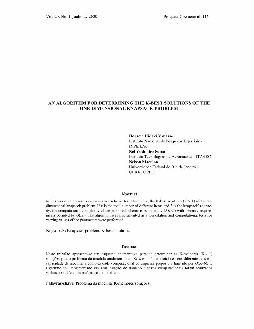
The proposed enumeration scheme is a recursive construction of optimal solutions to KPj for allpossible values of the right hand side j, from a1 up to b. It follows closely the one presented inYanasse and Soma [1987, 1990]. The method proposed can be viewed as an enumeration tree,where at each node we branch adding +1 to each one of the decision variables. So, for instance,at node t, we branch to get nodes t1, t2, …, tn, which are the result of adding 1 to xj, j = 1,..., nto the current solution at t (see Figure 1).

Figure 1Branching scheme

Following a path from the initial node (node 0) to any node t gives the values to be assigned tothe decision variables in order to reach node t. Observe that adding in sequence, +1 to xj, then +1to xk, ..., then +1 to xs or, by adding in sequence, +1 to xj, then +1 to xs, ..., then +1 to xk leadsto the same solution. Hence, to avoid duplications, when branching from a node t, it is sufficientto consider nodes corresponding to adding +1 to decision variables with indices greater than orequal to the index of the incoming branch at node t.

Further savings in the enumeration process are obtained by grouping nodes t and m into a supernode whenever the values of the knapsack constraint associated with these nodes are equal. Thishappens when t and m correspond to different combinations of the coefficients of the knapsackconstraint leading to the same value. That is, if the decision variables in the knapsack constrainttake the values obtained with the path from node zero to node t and with the path from node 0 tonode m, the corresponding values are equal.

- Pesquisa Operacional Vol. 20, No. 1, junho de2000__________________________________________________________________________________

120

Now, each super node t in the enumeration corresponds to the KPt. And, we know beforehandthat in our scheme we are interested in at most (b-a1) super nodes. From each super node t, weupdate n-j+1 new super nodes (“branching scheme”), where j is the smallest index in super node tfor which we know there is a solution for KPt, with xj ≥ 1. The super nodes to be updated are theones determined by adding to t, the coefficient ap, that is, super nodes (t+ap), p = j, j+1,..., n. Ofcourse, only super nodes of interest are updated, that is super nodes (t+ap) ≤ b. Observe that theabove operation corresponds to adding +1 to the variables with index p, p = j, j+1,...,n. Indicessmaller than j need not be considered since the corresponding combinations they produce areconsidered somewhere else. At each super node are kept the index j known to have at least onesolution for KPt with xj ≥ 1, together with its corresponding best solution. Observe that the bestsolution value at a super node (t+ap), corresponding to index p, is obtained by adding to the bestoptimal solution values at super node t corresponding to indices smaller than or equal to p, thecoefficient cp, p = j, j+1,...,n. Starting with super node t = 0, (the root super node, correspondingto KP0) with index set equal to {1,2,...,n} and corresponding objective values {0,0,...,0}, thesubsequent super nodes on which to “branch” are always chosen in increasing order of t. Onlysuper nodes having at least one solution are considered. Once a super node t > (b-a1) is reachedfor branching, we stop. The forward enumeration part has been finished.

We illustrate the forward enumeration scheme by means of a numerical example. Consider theKP:

Maximize z = 4x1+3x2+5x3+7x4+8x5

subject to 3x1+4x2+5x3+6x4+7x5 ≤ 15

xi ≥ 0 i = 1,2,...,5 and integer.

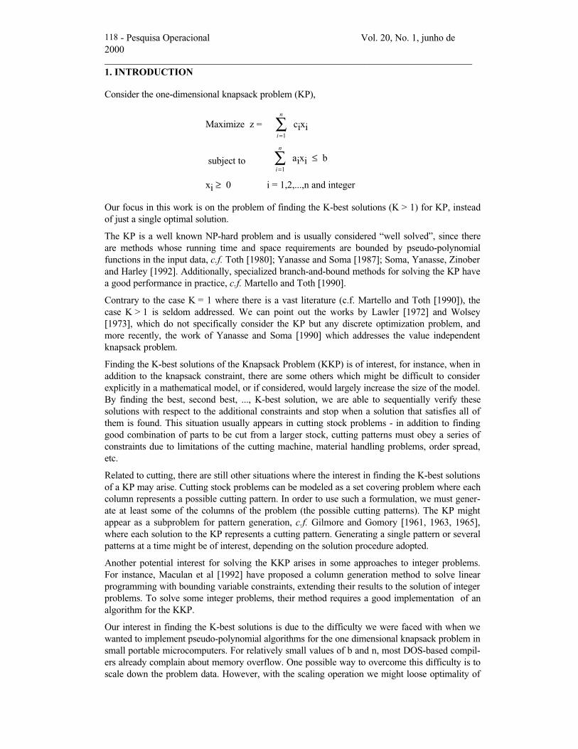
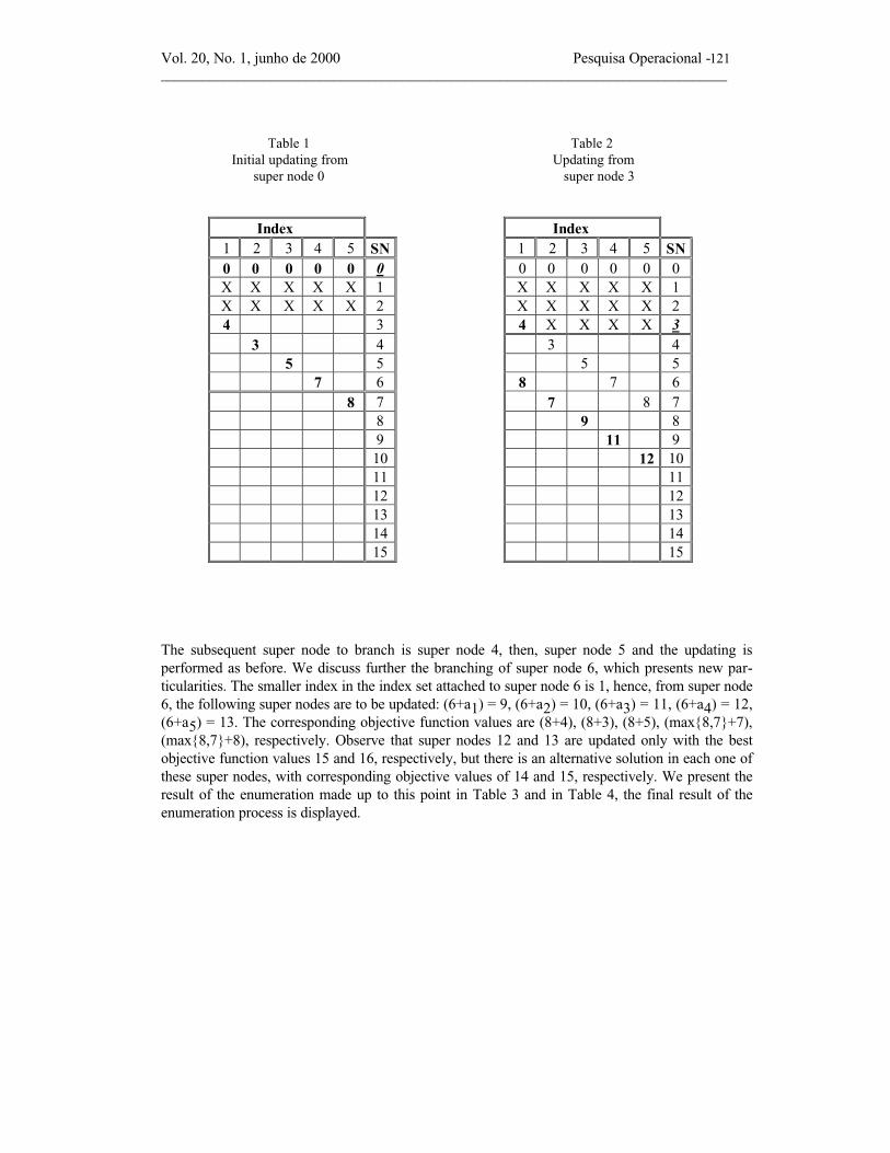
Initially, we start with super node 0, with an attached set of indices {1,2,3,4,5} and correspond-ing values of the objective function {0,0,0,0,0}. Nodes 3,4,...,15 are the other super nodes whoseset of indices and corresponding objective function values are to be updated. Observe that supernodes 1 and 2 (all super nodes t < a1) are never updated since they cannot be reached from supernode 0 (that is, there is no solution with right hand sides smaller than a1). Since the smaller in-dex in the index set attached to super node 0 is 1, from super node 0, the following super nodesare to be updated: (0+a1) = 3, (0+a2) = 4, (0+a3) = 5, (0+a4) = 6, (0+a5) = 7. The correspond-ing objective function values are (0+4), (max{0,0}+3), (max{0,0,0}+5), (max{0,0,0,0}+7),(max{0,0,0,0,0}+8), respectively. We represent this information in Table 1.

In Table 1, columns 1 to 5 give indication of the index attached to a super node. The super nodesare indicated in the last column. The numbers filled in the table in any column j are the best ob-jective values corresponding to a feasible solution having at least xj ≥ 1. For instance, column 4,node 6, has a value 7, indicating that there is a solution to KP6 with x4 ≥ 1 and correspondingobjective function value equal to 7.

The subsequent super node to branch is super node 3, which is the next super node after 0 thathas at least one solution. Since the smaller index in the index set attached to super node 3 is 1again, from super node 3, the following super nodes are to be updated: (3+a1) = 6, (3+a2) = 7,(3+a3) = 8, (3+a4) = 9, (3+a5) = 10. The corresponding objective function values are (4+4) ,(4+3), (4+5), (4+7), (4+8), respectively. This information is shown in Table 2.

Observe now in Table 2, that there are some rows (super nodes) with more than 2 objectivefunction values. This indicates a multiplicity of feasible solutions for the knapsack problem cor-responding to that super node. For instance, from row 6, we can conclude that KP6 has at least 2solutions with objective values 8 and 7 and one of the solutions has x1 ≥ 1 and the other x4 ≥ 1.

Vol. 20, No. 1, junho de 2000 Pesquisa Operacional -__________________________________________________________________________________

121

Table 1 Initial updating from super node 0

Table 2 Updating from super node 3

Index Index1 2 3 4 5 SN 1 2 3 4 5 SN0 0 0 0 0 0 0 0 0 0 0 0X X X X X 1 X X X X X 1X X X X X 2 X X X X X 24 3 4 X X X X 3

3 4 3 45 5 5 5

7 6 8 7 68 7 7 8 7

8 9 89 11 910 12 1011 1112 1213 1314 1415 15

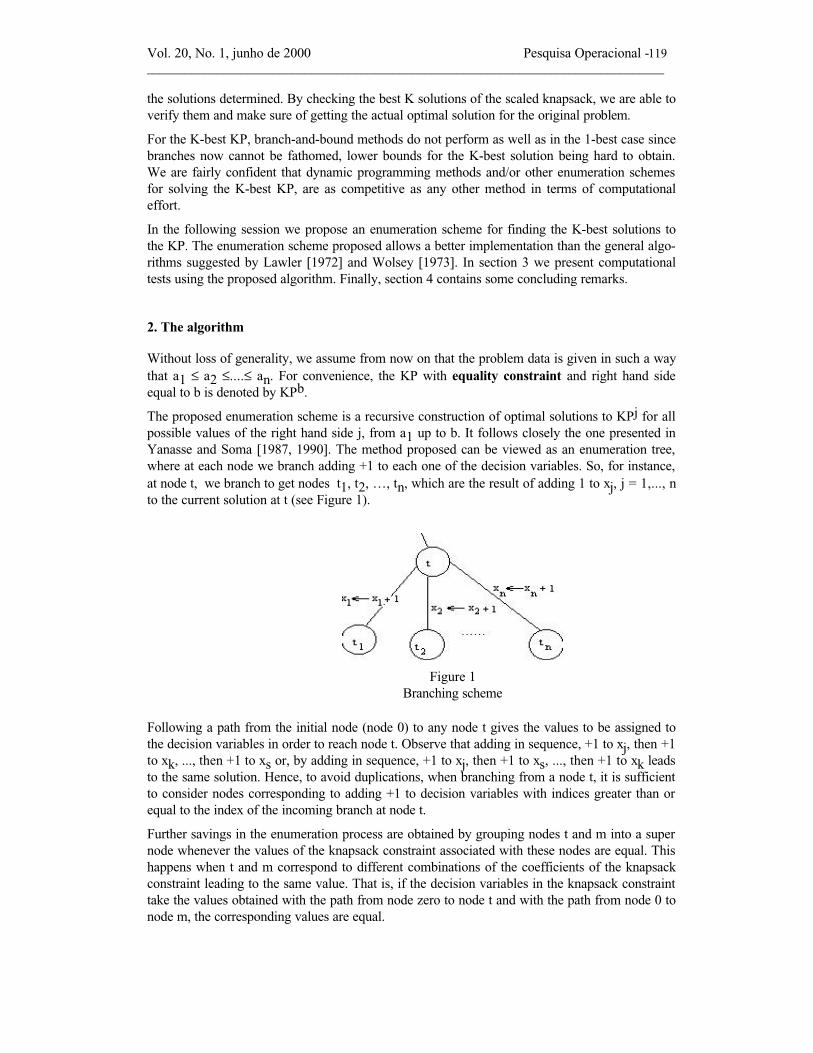
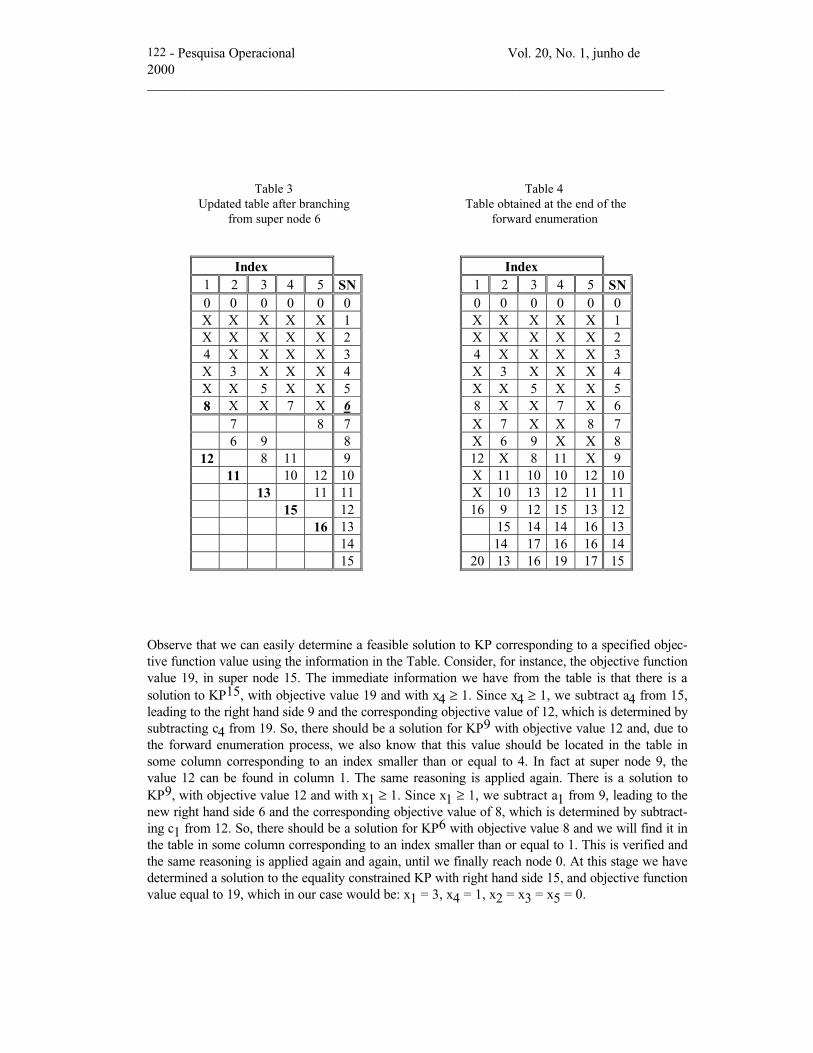
The subsequent super node to branch is super node 4, then, super node 5 and the updating isperformed as before. We discuss further the branching of super node 6, which presents new par-ticularities. The smaller index in the index set attached to super node 6 is 1, hence, from super node6, the following super nodes are to be updated: (6+a1) = 9, (6+a2) = 10, (6+a3) = 11, (6+a4) = 12,(6+a5) = 13. The corresponding objective function values are (8+4), (8+3), (8+5), (max{8,7}+7),(max{8,7}+8), respectively. Observe that super nodes 12 and 13 are updated only with the bestobjective function values 15 and 16, respectively, but there is an alternative solution in each one ofthese super nodes, with corresponding objective values of 14 and 15, respectively. We present theresult of the enumeration made up to this point in Table 3 and in Table 4, the final result of theenumeration process is displayed.

- Pesquisa Operacional Vol. 20, No. 1, junho de2000__________________________________________________________________________________

122

Table 3 Updated table after branching from super node 6

Table 4Table obtained at the end of the forward enumeration

Index Index1 2 3 4 5 SN 1 2 3 4 5 SN0 0 0 0 0 0 0 0 0 0 0 0X X X X X 1 X X X X X 1X X X X X 2 X X X X X 24 X X X X 3 4 X X X X 3X 3 X X X 4 X 3 X X X 4X X 5 X X 5 X X 5 X X 58 X X 7 X 6 8 X X 7 X 6

7 8 7 X 7 X X 8 76 9 8 X 6 9 X X 8

12 8 11 9 12 X 8 11 X 911 10 12 10 X 11 10 10 12 10

13 11 11 X 10 13 12 11 1115 12 16 9 12 15 13 12

16 13 15 14 14 16 1314 14 17 16 16 1415 20 13 16 19 17 15

Observe that we can easily determine a feasible solution to KP corresponding to a specified objec-tive function value using the information in the Table. Consider, for instance, the objective functionvalue 19, in super node 15. The immediate information we have from the table is that there is asolution to KP15, with objective value 19 and with x4 ≥ 1. Since x4 ≥ 1, we subtract a4 from 15,leading to the right hand side 9 and the corresponding objective value of 12, which is determined bysubtracting c4 from 19. So, there should be a solution for KP9 with objective value 12 and, due tothe forward enumeration process, we also know that this value should be located in the table insome column corresponding to an index smaller than or equal to 4. In fact at super node 9, thevalue 12 can be found in column 1. The same reasoning is applied again. There is a solution toKP9, with objective value 12 and with x1 ≥ 1. Since x1 ≥ 1, we subtract a1 from 9, leading to thenew right hand side 6 and the corresponding objective value of 8, which is determined by subtract-ing c1 from 12. So, there should be a solution for KP6 with objective value 8 and we will find it inthe table in some column corresponding to an index smaller than or equal to 1. This is verified andthe same reasoning is applied again and again, until we finally reach node 0. At this stage we havedetermined a solution to the equality constrained KP with right hand side 15, and objective functionvalue equal to 19, which in our case would be: x1 = 3, x4 = 1, x2 = x3 = x5 = 0.

Vol. 20, No. 1, junho de 2000 Pesquisa Operacional -__________________________________________________________________________________

123

Recovering the K-best solutions

To recover the K-best solutions a list of the K-best objective function values to the KP is built bytraversing the super nodes from b, b-1,...,0, and by choosing the K-best solution values. Unfortu-nately, they are not always the K-best solutions to our KP. There might be alternative solutionswith the same objective function value or a little bit smaller which are not explicitly indicated inthe final table. It is necessary, therefore, to check the existence of any other alternative solutionbetter than the Kth element listed so far. The only thing that can be stated at this point is that theKth element in the list is just a lower bound for the K-best optimal solution value of the KP.

In our previous numerical example, let us assume K = 15. The initial list containing the best K(=15) objective function values to the KP are: 20, 19, 17, 17, 16, 16, 16, 16, 16, 15, 15, 14, 14,14 and 13. Hence, a lower bound on the 15th-best objective function value is 13 and a checkverifying whether there are other solutions, not explicitly indicated in the final enumeration table,better than the Kth solution, is, then, performed.

The recovering of the K-best solutions is achieved by analyzing the solutions corresponding to thebest K values already identified in the list. In the process, we search for alternative solutionshaving objective values better than the Kth best value identified so far. Our search will startanalyzing the best, second best, third best and so on solutions, hoping that by analyzing first thebest solutions, there would be an increased chance of finding alternative solutions as good as theones being considered. Once the analysis of a Jth-best solution with value equal to the Kth best inthe list is reached we can stop. The K-best solution values are now at hand and it is necessaryonly to determine the remaining solutions corresponding to the objective values in the list, whichwere not considered yet.

Alternative solutions are identified in the process of recovering a solution to a specific objectivevalue, whenever more than one feasible solution is observed in any intermediate super node dur-ing backtracking. For instance, in the previous recovering process example with super node 15and objective value 19, a backtrack in super node 9 detected 3 solutions with objective values(12,8,11) identified in the table. All three of them are feasible in the sense that super node 15 canbe reached from them and moreover, a numerical value in column 4 indicates that all these valuesare in columns with indices smaller than or equal to 4. Hence, with all of them, by adding +1 tovariable x4, leads to super node 15, column 4. In this example, the objective values correspond-ing to these alternative solutions are different: 19, 15 and 18, respectively. Only one of the solu-tions reaches the value 19, the best value with at least one x4 ≥ 1.

The full recovery of the 15-best solutions of our numerical example is illustrated now. The proc-ess starts with the 1-best solution value 20. Backtracking, it is seen that the value 20 in supernode 15 came by adding +1 to variable x1. Subtracting a1 from 15 yields super node 12, withcorresponding objective value of 16 = 20 - c1.

We are again in a similar situation and proceed in the same way, concluding that there is no al-ternative solution for this case. The single solution x1 = 5, x2 = x3 = x4 = x5 = 0, with objectivefunction value 20 has been obtained.

The next solution to be considered is the second best one, whose objective function value is 19.As previously pointed out, there are alternative solutions in this case. Recall that with the back-tracking from super node 15, solution value 19, super node 9 was reached with alternative solu-tions. In the process of analyzing these alternative solutions, we start with the largest indexsmaller than or equal to 4. A solution of value 11 is found at column 4 in row 9, indicating that asolution exists with corresponding objective function value of 18. This value is compared with thecurrent 15th-best value in the list to see if this solution will be included among the 15-best or is tobe discarded. In this case, a better solution has been obtained, hence, this value is introduced inthe list and the previous 15th value is deleted. With the new list, the lower bound for the 15th-best solution is updated and the process is repeated from where it has been previously halted, i.e.

- Pesquisa Operacional Vol. 20, No. 1, junho de2000__________________________________________________________________________________

124

from super node 9, column 4 and objective value 11. We backtrack subtracting a4 from 9. Thisgives super node 3 with corresponding objective value 4. There is a single solution in node 3 andproceeding with the backtracking up to super node 0 a solution is identified, given by x1 = 1, x4= 2, x2 = x3 = x5 = 0, with corresponding objective value 18.

Then we return to the smallest super node where an alternative solution was identified, supernode 9 in this case. It is necessary now to move to the immediate next column with a smallerindex with a solution, that is column 3. A solution of value 8 is found, indicating that a solutionexists with corresponding objective function value of 15. Again, this value is compared with the15th-best value in the list, and since this latter one is greater than the former, it is, therefore,introduced in the list and the previous 15th value is discarded. The lower bound for the 15th-bestsolution is updated and the process is re-launched from where it has stopped.

Since the last super node considered was the 9, column 3, with objective value 8 a backtrackingis performed by subtracting a3 from 9, reaching super node 4 with corresponding objective valueof 3. There is just a single solution in super node 4 and proceeding with the backtracking up tosuper node 0 the solution x2 = 1, x3 = 1, x4 = 1, x1 = x5 = 0, with corresponding objectivevalue 15 is identified.

The smallest super node where an alternative solution was identified, i.e. super node 9 is consid-ered again and the immediate next column, which has yet to be considered, with a smaller indexpossessing a solution is column 1. A solution of value 12 is found, and after a backtracking nomore alternative solutions are found, and the single solution x1 = 3, x4 = 1, x2 = x3 = x5 = 0,with corresponding objective function value of 19 is identified.

We move now to the next best value in the list not yet analyzed. At this stage, the list haschanged to 20*, 19*, 18*, 17, 17, 16, 16, 16, 16, 16, 15*, 15, 15, 14, 14, where the values indi-cated with an * are the ones which have already been analyzed (the corresponding solutions havealready been obtained). The third best value in the list is 18 and it was considered during theanalysis of the 2nd best value. Hence, the 4th-best value, which is 17, is considered next.

Proceeding with the same reasoning, we are in super node 15, column 5, objective value 17, andthe backtracking implies in subtracting a5 from 15, reaching super node 8 which has two solu-tions. Starting again the recovering process with the largest index smaller than or equal to 5, asolution of value 9 is found at column 3 in row 8, indicating a solution with corresponding ob-jective function value of 17. We backtrack subtracting a3 from 8 to reach super node 3 withcorresponding objective value 4. There is a single solution in node 3 and proceeding with thebacktracking up to super node 0 the solution x1 = 1, x3 = 1, x5 = 1, x2 = x4 = 0 is identified,with corresponding objective value 17.

Returning to the smallest super node where an alternative solution was identified, super node 8,we move to the immediate next column with a smaller index with a solution, that is column 2. Asolution of value 6 is found indicating a solution with corresponding objective function of 14.Since this is worse than the 15th-best value in the current list, this solution is discarded. No morealternative solution are present, we then move to the 5th-best value of the list, which is again 17.

This is in super node 14, column 3, objective value 17, and a backtracking is carried out by sub-tracting a3 from 14 reaching super node 9. In this super node there are 3 solutions,. however,only two of them with indices smaller than or equal to 3. Starting with the largest index smallerthan or equal to 3, a solution of value 8 is found at column 3 in row 9, indicating a solution withcorresponding objective function of 13. Since this is worse than the 15th best current value, thissolution is disregarded and the next alternative solution is examined. Moving to the immediatenext column with a smaller index and with a solution, that is column 1, a solution of value 12 isfound indicating a solution with corresponding objective function of 17. Since this solution isbetter than the 15th best in the list, we proceed with the backtracking, arriving at the solution x1

Vol. 20, No. 1, junho de 2000 Pesquisa Operacional -__________________________________________________________________________________

125

= 3, x3 = 1, x2 = x4 = x5 = 0, with corresponding objective value 17. No more alternative solu-tions are present, so the 6th-best value of the list, which is 16, is examined next.

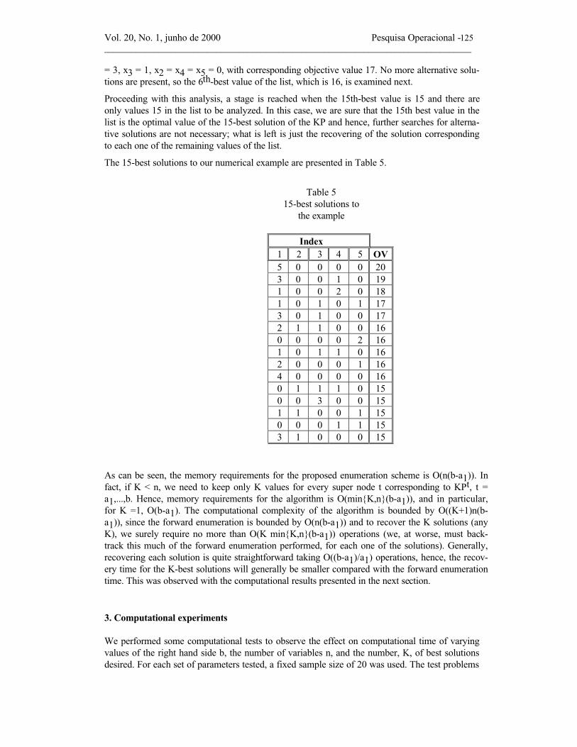
Proceeding with this analysis, a stage is reached when the 15th-best value is 15 and there areonly values 15 in the list to be analyzed. In this case, we are sure that the 15th best value in thelist is the optimal value of the 15-best solution of the KP and hence, further searches for alterna-tive solutions are not necessary; what is left is just the recovering of the solution correspondingto each one of the remaining values of the list.

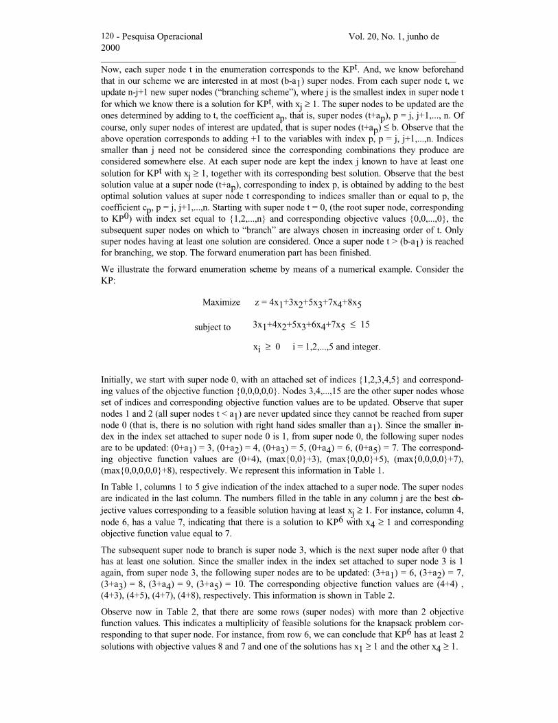
The 15-best solutions to our numerical example are presented in Table 5.

Table 515-best solutions to

the example

Index1 2 3 4 5 OV5 0 0 0 0 203 0 0 1 0 191 0 0 2 0 181 0 1 0 1 173 0 1 0 0 172 1 1 0 0 160 0 0 0 2 161 0 1 1 0 162 0 0 0 1 164 0 0 0 0 160 1 1 1 0 150 0 3 0 0 151 1 0 0 1 150 0 0 1 1 153 1 0 0 0 15

As can be seen, the memory requirements for the proposed enumeration scheme is O(n(b-a1)). Infact, if K < n, we need to keep only K values for every super node t corresponding to KPt, t =a1,...,b. Hence, memory requirements for the algorithm is O(min{K,n}(b-a1)), and in particular,for K =1, O(b-a1). The computational complexity of the algorithm is bounded by O((K+1)n(b-a1)), since the forward enumeration is bounded by O(n(b-a1)) and to recover the K solutions (anyK), we surely require no more than O(K min{K,n}(b-a1)) operations (we, at worse, must back-track this much of the forward enumeration performed, for each one of the solutions). Generally,recovering each solution is quite straightforward taking O((b-a1)/a1) operations, hence, the recov-ery time for the K-best solutions will generally be smaller compared with the forward enumerationtime. This was observed with the computational results presented in the next section.

3. Computational experiments

We performed some computational tests to observe the effect on computational time of varyingvalues of the right hand side b, the number of variables n, and the number, K, of best solutionsdesired. For each set of parameters tested, a fixed sample size of 20 was used. The test problems

- Pesquisa Operacional Vol. 20, No. 1, junho de2000__________________________________________________________________________________

126

were constructed artificially with all coefficients aj of the knapsack constraint generated ran-domly in the interval [1,5000].

Our proposed enumeration scheme was implemented in C++ on an IBM RISC/6000, Model580H, with an IBM Power PC 2 processor and 256 Mbytes of RAM memory. All processingtimes were measured in seconds.

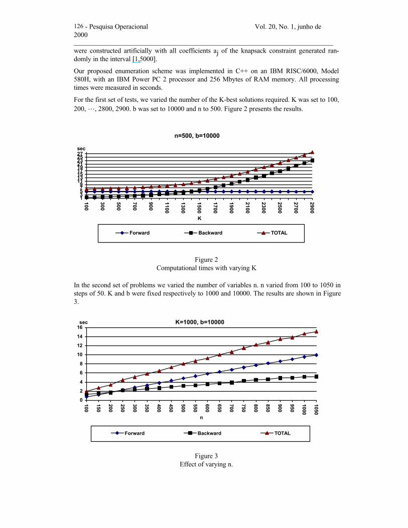
For the first set of tests, we varied the number of the K-best solutions required. K was set to 100,200, L, 2800, 2900. b was set to 10000 and n to 500. Figure 2 presents the results.

n=500, b=10000

13579111315171921232527

100

300

500

700

900

1100

1300

1500

1700

1900

2100

2300

2500

2700

2900

K

sec

Forward Backward TOTAL

Figure 2Computational times with varying K

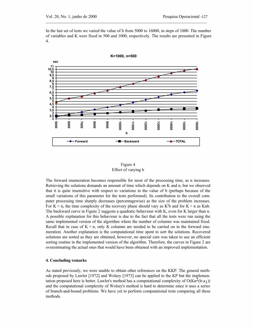
In the second set of problems we varied the number of variables n. n varied from 100 to 1050 insteps of 50. K and b were fixed respectively to 1000 and 10000. The results are shown in Figure3.

K=1000, b=10000

0

2

4

6

8

10

12

14

16100

150

200

250

300

350

400

450

500

550

600

650

700

750

800

850

900

950

1000

1050

n

sec

Forward Backward TOTAL

Figure 3Effect of varying n.

Vol. 20, No. 1, junho de 2000 Pesquisa Operacional -__________________________________________________________________________________

127

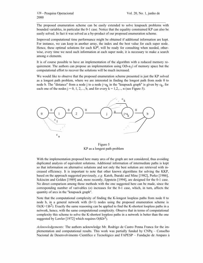
In the last set of tests we varied the value of b from 5000 to 16000, in steps of 1000. The numberof variables and K were fixed in 500 and 1000, respectively. The results are presented in Figure4.

K=1000, n=500

22,5

33,5

44,5

55,5

66,5

77,5

88,5

99,510

10,511

5000

6000

7000

8000

9000

10000

11000

12000

13000

14000

15000

16000

b

sec

Forward Backward TOTAL

Figure 4Effect of varying b

The forward enumeration becomes responsible for most of the processing time, as n increases.Retrieving the solutions demands an amount of time which depends on K and n, but we observedthat it is quite insensitive with respect to variations in the value of b (perhaps because of thesmall variations of this parameter for the tests performed). Its contribution to the overall com-puter processing time sharply decreases (percentagewise) as the size of the problem increases.For K < n, the time complexity of the recovery phase should vary as K2b and for K > n as Knb.The backward curve in Figure 2 suggests a quadratic behaviour with K, even for K larger than n.A possible explanation for this behaviour is due to the fact that all the tests were run using thesame implemented version of the algorithm where the number of columns was maintained fixed.Recall that in case of K < n, only K columns are needed to be carried on in the forward enu-meration. Another explanation is the computational time spent to sort the solutions. Recoveredsolutions are sorted as they are obtained, however, no special care was taken to use an efficientsorting routine in the implemented version of the algorithm. Therefore, the curves in Figure 2 areoverestimating the actual ones that would have been obtained with an improved implementation.

4. Concluding remarks

As stated previously, we were unable to obtain other references on the KKP. The general meth-ods proposed by Lawler [1972] and Wolsey [1973] can be applied to the KP but the implemen-tation proposed here is better. Lawler's method has a computational complexity of O(Kn2(b-a1))and the computational complexity of Wolsey's method is hard to determine since it uses a seriesof branch-and-bound problems. We have yet to perform computational tests comparing all thesemethods.

- Pesquisa Operacional Vol. 20, No. 1, junho de2000__________________________________________________________________________________

128

The proposed enumeration scheme can be easily extended to solve knapsack problems withbounded variables, in particular the 0-1 case. Notice that the equality constrained KP can also beeasily solved. In fact it was solved as a by-product of our proposed enumeration scheme.

Improved computational time performance might be obtained if additional information are kept.For instance, we can keep in another array, the index and the best value for each super node.Hence, these optimal solutions for each KPt, will be ready for consulting when needed, other-wise, every time we need such information at each super node, it is necessary to make a searchamong n elements.

It is of course possible to have an implementation of the algorithm with a reduced memory re-quirement. The authors can propose an implementation using O(b-a1) of memory space but thecomputational effort to recover the solutions will be much increased.

We would like to observe that the proposed enumeration scheme presented is just the KP solvedas a longest path problem, where we are interested in finding the longest path from node 0 tonode b. The "distance" from a node j to a node j+ak in the "knapsack graph" is given by ck, foreach one of the nodes j = 0, 1, 2,..., b, and for every k = 1,2,..., n (see Figure 5).

0 1 2 j j+a bk

ck

c1

cn

0 0 00

0

..

.

..

.

..

.

Figure 5 KP as a longest path problem

With the implementation proposed here many arcs of the graph are not considered, thus avoidingduplicated analysis of equivalent solutions. Additional information of intermediate paths is keptso that information on alternative solutions and not only the best solution are retrieved with in-creased efficiency. It is important to note that other known algorithms for solving the KKP,based on the approach suggested previously, e.g. Katoh, Ibaraki and Mine [1982], Perko [1986],Sckiscim and Golden [1989] and, more recently, Eppstein [1994], are designed for the 0-1 case.No direct comparison among those methods with the one suggested here can be made, since thecorresponding number of varivables (n) increases for the 0-1 case, which, in turn, affects thequantity of arcs in the "knapsack graph".

Note that the computational complexity of finding the K-longest loopless paths from node 0 tonode b, in a general network with (b+1) nodes using the proposed enumeration scheme isO((K+1)b2). Exactly the same reasoning can be applied to find the K-shortest loopless paths in anetwork, hence, with the same computational complexity. Observe that in terms of computationalcomplexity this scheme to solve the K-shortest loopless paths in a network is better than the onesuggested by Lawler [1972] which requires O(Kb3).

Acknowledgements: The authors acknowledge Mr. Rodrigo de Castro Penna Franca for the im-plementation and computational results. This work was partially funded by CNPq – ConselhoNacional de Desenvolvimento Científico e Tecnológico and FAPESP – Fundação de Amparo à

Vol. 20, No. 1, junho de 2000 Pesquisa Operacional -__________________________________________________________________________________

129

Pesquisa do Estado de São Paulo. The authors also thanks for the comments of the anonymousreferees that improved the presentation of the paper.

References

(1) Eppstein, D. (1994) Finding the k Shortest Paths, Proc. 25th IEEE Annual Symposium onFoundation of Computer Science, 154-165.

(2) Gilmore, P.; Gomory, R. (1961) A linear programming approach to the cutting stock prob-lem. Operations Research, 9, 849-859.

(3) Gilmore, P.; Gomory, R. (1963) A linear programming approach to the cutting stock problem- part II. Operations Research, 11, 863-888.

(4) Gilmore, P.; Gomory, R. (1965) Multistage cutting stock problems of two and more dimen-sions. Operations Research, 14, 1045-1074.

(5) Katoh, N.; Ibaraki, T.; Mine, H. (1982) An efficient algorithm for the shortest simple paths,Networks, 12, 411-448.

(6) Lawler, E.L. (1972) A procedure for computing the k-best solutions to discrete optimizationproblems and its application to the shortest path problem. Management Science, 18 (7), 401-405.

(7) Maculan, N.; Michelon, P.; Plateau, G. (1992) Column-generation in linear programmingwith bounding variable constraints and its application in integer programming. Pesquisa Op-eracional, 12 (2), 45-57.

(8) Perko A. (1986) Implementations of algorithms for k shortest loopless paths, Networks, 16,149-160.

(9) Martello, S.; Toth, P. (1990) Knapsack problems - Algorithms and Computer Implementa-tions. John Wiley & Sons, Chichester.

(10) Sckiscim C.C. and Golden, B.L. (1989) Solving k-shortest and constrained shortest pathproblems efficiently, Annals of Operations Research, 20, 249-282.

(11) Soma, N.Y.; Yanasse, H.H.; Zinober, A.S.I.; Harley, P. J. (1992) A pseudopolylogarithmicalgorithm for the subset sum problem. CO92 - Combinatorial Optimization Conference, Uni-versity of Oxford, Oxford, England.

(12) Toth, P. (1980) Dynamic programming algorithms for the zero-one knapsack problem,Computing, 25, 29-45.

- Pesquisa Operacional Vol. 20, No. 1, junho de2000__________________________________________________________________________________

130

(13) Wolsey, L.A. (1973) Generalized dynamic programming methods in integer programming.Mathematical Programming, 4, 222-232.

(14) Yanasse, H.H.; Soma, N.Y. (1987) A new enumeration scheme for the knapsack problem.Discrete Applied Mathematics, 18, 235-245.

(15) Yanasse, H.H.; Soma, N.Y. (1990) Finding the k-best solutions to a value independentknapsack problem. IFORS XII, Athens, Greece.

Appendix – The K-best algorithm

Givenpositive integers b, n, K, ai, i = 1, 2, ..., n,

such thatn ≤ K and a1 ≤ a2 ≤....≤ an,

non-negative real numbers ci, i = 1, 2, ..., n. If for some i, ai = ai+1 then ci ≥ ci+1.Notation• Variables in bold indicate vectors;• 0 is a vector with all components equal to 0.• 1 is a vector with all components equal to 1.• // line with comments

The algorithm

Main ProgramBegin-Main// Begin-Initialization

Generate matrix MbXn

M(r,s) ← -1, r = 1,...,b and s = 1,...,n// End-Initialization

// Begin-Forward Enumeration// Begin initial ramification

For j = 1 to n do M(aj,j) ← cj;// End-initial ramification// Begin-ramification of supernodes

For t = a1 to (b - a1) doBegin-For

m ← n+1;m ← min {i : M(t,i) ≥ 0, i = 1, … n};If (m ≠ n+1) ThenBegin If

z ← M(t,m);For i = m to n do

Begin-ForIf (t+ai) ≤ b ThenBegin-If

Vol. 20, No. 1, junho de 2000 Pesquisa Operacional -__________________________________________________________________________________

131

If (M(t,i) > z) Then z ← M(t,i);M(t+ai,i) ← z+ci;

End-If End-ForEnd-If

End-For// End-ramification of supernodes

// End-Forward Enumeration// Begin-Backward Recovering

Execute Build-initial-best-K-list (L,P,K)// P is equal to K if there are at least K best values available; L(i) is the ith best solution in// the list and is characterized by 5 attributes: L(i).X the vector solution, L(i).V the// objective function value, L(i).J and L(i).T which are, respectively, the original column// and line in matrix MbXn where the solution was identified, and L(i).C, an 0-1 control// variable that indicates whether the vector solution L(i).X has already been// recovered or not.Execute Recover-solution (L,P,K)

// End-Backward RecoveringEnd-Main

Procedure Build-initial-best-K-list (L,P,K)Begin // Build-initial-best-K-list// List of K elements are ordered at a time. Lists are combined when necessary. Many other// alternative ways to find the initial K-best elements exist (e.g. Binary Search Tree// with post-order)

Counter ← 0;i ← b+1;Fim ← False;Moreleft ← False;While (i > a1) doBegin-While

i ← i-1;j ← n+1;While (j > 1) doBegin-While

j ← j-1;If (M(i,j) ≥ 0) ThenBegin-If

Counter ← Counter + 1;L(Counter).V ← M(i,j);L(Counter).J ← j;L(Counter).T ← i;If (Counter = K) ThenBegin-If

i1 ← i;j1 ← j;Moreleft ← True;i ← 0;j ← 0;

End-If

- Pesquisa Operacional Vol. 20, No. 1, junho de2000__________________________________________________________________________________

132

End-IfEnd-While

End-WhileP ← Counter;Sort in non-increasing order, L(i) i = 1, ..., P, using attribute L(i).VIf ((P = K).AND.(( i1 > a1).OR.( j1 > 1)) Then Fim ← True;While (Fim) doBegin-While

Counter ← 0;i ← i1+1;Fim ← False;While (i > a1) doBegin-While

i ← i-1;j ← n+1;If (Moreleft) ThenBegin-If

j ← j1;Moreleft ← False;

End-IfWhile (j > 1) doBegin-While

j ← j-1;If (M(i,j) > L(K).V ) ThenBegin-If

Counter ← Counter + 1;L1(Counter).V ← M(i,j);L1(Counter).J ← j;L1(Counter).T ← I;If (Counter = K) ThenBegin-If

i1 ← i;j1 ← j;Moreleft ← True;i ← 0;j ← 0;

End-IfEnd-If

End-WhileEnd-WhileP1 ← Counter;Sort in non-increasing order, L1(i) i = 1, ..., P1, using attribute L1(i).VIf (L1(1).V > L(K).V) Then using lists L and L1, build a sorted list (non-increasing or-

der) of the K objects having the largest V attribute. Assign this list to L(i), i = 1, ..., K;If (( i1 > a1).OR.( j1 > 1)) Then Fim ← True;

End-WhileFor i = 1 to P doBegin-For

L(i).X ← 0;L(i).C ← 0;

End-For

Vol. 20, No. 1, junho de 2000 Pesquisa Operacional -__________________________________________________________________________________

133

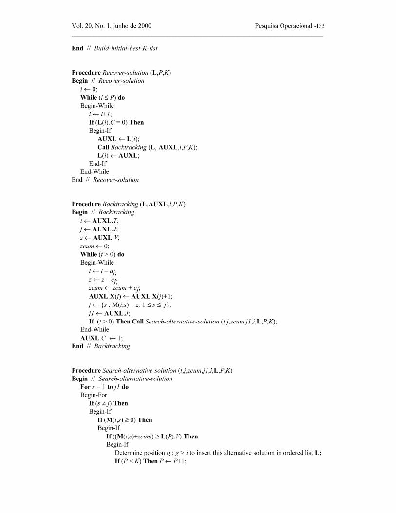
End // Build-initial-best-K-list

Procedure Recover-solution (L,P,K)Begin // Recover-solution

i ← 0;While (i ≤ P) doBegin-While

i ← i+1;If (L(i).C = 0) ThenBegin-If

AUXL ← L(i);Call Backtracking (L, AUXL,i,P,K);L(i) ← AUXL;

End-IfEnd-While

End // Recover-solution

Procedure Backtracking (L,AUXL,i,P,K)Begin // Backtracking

t ← AUXL.T;j ← AUXL.J;z ← AUXL.V;zcum ← 0;While (t > 0) doBegin-While

t ← t – aj;z ← z – cj;zcum ← zcum + cj;AUXL.X(j) ← AUXL.X(j)+1;j ← {s : M(t,s) = z, 1 ≤ s ≤ j};j1 ← AUXL.J;If (t > 0) Then Call Search-alternative-solution (t,j,zcum,j1,i,L,P,K);

End-WhileAUXL.C ← 1;

End // Backtracking

Procedure Search-alternative-solution (t,j,zcum,j1,i,L,P,K)Begin // Search-alternative-solution

For s = 1 to j1 doBegin-For

If (s ≠ j) ThenBegin-If

If (M(t,s) ≥ 0) ThenBegin-If

If ((M(t,s)+zcum) ≥ L(P).V) ThenBegin-If

Determine position g : g > i to insert this alternative solution in ordered list L;If (P < K) Then P ← P+1;

- Pesquisa Operacional Vol. 20, No. 1, junho de2000__________________________________________________________________________________

134

f ← P;While (f > g) doBegin-While L(f) ← L(f-1); f ← f-1;End-WhileL(g).V ← M(t,s) + zcum;L(g).J ← L(i).J;L(g).T ← L(i).T;AUXL1.V ← M(t,s);AUXL1.J ← s;AUXL1.T ← t;AUXL1.X ← 0;Call Backtracking (L,AUXL1,g,P,K);L(g).C ← 1;L(g).X ← L(i).X + AUXL1.X;If (M(t,s) ≥ L(P).V) ThenBegin-If

Determine position k : k > g to insert this alternative solution in ordered list L;If (P < K) Then P ← P+1;f ← P;While (f > k) doBegin-While

L(f) ← L(f-1);f ← f-1;

End-WhileL(k) ← AUXL1;

End-IfEnd-If

End-IfEnd-If

End-ForEnd // Search-alternative-solution