An aggregation-based solution method forM/G/1-type processesGianfranco Ciardo Alma Riska Evgenia Smirni?Department of Computer ScienceCollege of William and MaryWilliamsburg, VA 23187-8795, USAfciardo,riska,esmirnig@cs.wm.eduAbstract. We extend the ETAQA approach, initially proposed for thee�cient numerical solution of a class of quasi birth-death processes, tothe more complex case of M/G/1-type Markov processes. The proposedtechnique can be used for the exact solution of a class of M/G/1-typemodels by computing the solution of a �nite linear system. We furtherdemonstrate the utility of the method by describing the exact computa-tion of an extensive set of Markov reward functions such as the expectedqueue length or its higher moments. We illustrate the method, discuss itscomplexity, present comparisons with other traditional techniques, andillustrate its applicability in the area of computer system modeling.1 IntroductionWe consider Markov chains on an in�nite state space having a M/G/1-typestructure. Such processes often serve as the modeling tool of choice for mod-ern computer and communication systems [7]. As a consequence, considerablee�ort has been placed into the development of exact analysis techniques forM/G/1-type processes. The in�nitesimal generator of such processes (for thecase of continuous time Markov chains) is upper block Hessenberg and follows arepetitive structure. Matrix-analytic methods have been proposed for their so-lution, the best known probably being the one developed by Neuts [9]. The keyin the matrix-analytic solution is the computation of an auxiliary matrix calledG. Similarly, for Markov chains the of GI/M/1-type, which have a lower blockHessenberg form, matrix-geometric solutions have been proposed [8]. Again, thekey in the matrix-geometric solution is the computation of an auxiliary matrix,called R. Traditionally, iterative procedures are used for the determination ofboth matrices. Alternative algorithms for the computation of G (and R) havebeen proposed (e.g., the work of Latouche [4] for the e�cient computation of R;the same algorithms can be used to compute the matrix G [4]). Other methodsfor the computation of G (and R) using a recursive descent method have beenproposed [14] and compared with the traditional methods [5].The primary distinction between our research and the above works is that werestrict our attention to a family of M/G/1-type processes with a speci�c form,? This research has been supported by a William and Mary Summer Research Grant.

for which \returns" from a higher level of states to the immediate lower level arealways directed toward a single state (for such a subclass, the computation of thematrixG is trivial, but the remaining solution steps using standard methods arestill expensive). We instead recast the problem to the one of solving a �nite linearsystem of m + 2n equations where m is the number of states in the boundaryportion of the process and n is the number of states in each of the repetitive\levels" of the state space, and are able to obtain \exact" results.Our approach is an extension of the ETAQA method we introduced for thee�cient solution of quasi-birth-death processes with matrix-geometric form [2].The proposed methodology uses basic well-known results for Markov chains.We exploit the structure of the repetitive portion of the chain and instead ofevaluating the probability distribution of all states in the chain, we calculate theaggregate probability distribution of n equivalence classes, appropriately de�ned.The extended ETAQA approach is both e�cient and exact, allowing us to com-pute the probabilities of the boundary states as well as the aggregate probabilityof the n equivalence classes; it also provides the ability to e�ciently compute theexpected reward rates of interests, such as the kth moment of the queue length.This paper is organized as follows. Sect. 2 presents terminology and describesthe use of ETAQA for the solution of quasi-birth-death processes. In Sect. 3 wepresent the basic theorem that extends ETAQA to M/G/1-type processes. Wedemonstrate how the methodology can be used for the computation of Markovreward functions in Sect. 4. We continue by showing the applicability of extendedETAQA to bounded bulk arrivals in Sect. 5. In Sect. 6 we compare the compu-tation and storage complexity of the extended ETAQA with Neuts's algorithm[9] for the analysis of M/G/1 processes. Sect. 7 presents two applications fromthe computer systems area that can be analyzed using the extended ETAQA.Finally, Sect. 8 summarizes our �ndings and outlines future work.2 Using ETAQA for the solution of QBD processesWe brie y review the terminology used to describe the class of processes weconsider, and our previous results on ETAQA. We restrict ourselves to the caseof continuous-time Markov chains (hence we refer to the in�nitesimal generatormatrix Q), but the theory can just as well be applied to the discrete case.2.1 Markov chains with repetitive structureNeuts [8] de�nes various classes of in�nite-state Markov chains with a repetitivestructure. In all cases, the state space is partitioned into the boundary statesS(0) = fs(0)1 ; : : : ; s(0)m g and the sets of states S(j) = fs(j)1 ; : : : ; s(j)n g, for j � 1.For GI/M/1-type and M/G/1-type Markov chains, the in�nitesimal generatorQ can be block-partitioned, respectively, as:26666664 L(0) F 0 0 0 0 � � �B(1) L F 0 0 0 � � �B(2) B(1) L F 0 0 � � �B(3) B(2) B(1) L F 0 � � �... ... ... ... ... ... . . .37777775 and 2666664L(0) F(1) F(2) F(3) F(4) F(5) � � �B L F(1) F(2) F(3) F(4) � � �0 B L F(1) F(2) F(3) � � �0 0 B L F(1) F(2) � � �... ... ... ... ... ... . . .

3777775 :

For quasi-birth-death (QBD) Markov chains, which is the intersection of the twoprevious cases, the in�nitesimal generator Q can be block-partitioned as:2666664L(0) F 0 0 0 0 � � �B L F 0 0 0 � � �0 B L F 0 0 � � �0 0 B L F 0 � � �... ... ... ... ... ... . . .3777775 ;(we use the letter \L", \F", and \B" according to whether the matrices describe\local", `forward", and \backward" transition rates, respectively, and we use a\ " for matrices related to S(0)).The matrix-geometric approach [8] can be used to study GI/M/1-type pro-cesses. If �(j) is the stationary probability vector for states in S(j), we have:8j � 1; �(j) = �(1) �Rj�1; (1)where R is the solution of the matrix equationF+R � L+ 1Xk=1Rk+1 �B(k) = 0Iterative numerical algorithms can be used to compute R. Then, we can write[�(0);�(1)] � � L(0) F(1)P1k=1Rk�1 � B(k) L+P1k=1Rk �B(k) � = 0which, together with the normalization condition�(0) � 1T + �(1) � 1Xj=1Rj�1 � 1T = 1 i.e., �(0) � 1T + �(1) � (I�R)�1 � 1T = 1;yields a unique solution for �(0) and �(1). For j � 2, �(j) can be obtainednumerically from (1). More importantly, though, many useful performance met-rics, such as expected system utilization, throughput, or queue length, can becomputed exactly in explicit form from �(0), �(1), and R alone.2.2 ETAQAThe matrix-geometric approach is directly applicable to QBD processes as well,since QBD processes are a special case of GI/M/1-type processes. In [2] wepresented ETAQA, an alternative approach that can be used to solve a subclassof QBD processes more e�ciently than the classic matrix geometric technique.To apply ETAQA, B must contain nonzero entries in only one of its columns(which by convention we number last, n). This e�ectively means that all tran-sitions from S(j) to S(j�1) are restricted to go to s(j�1)n . When this conditionholds, it is possible to derive a system of m + 2n independent linear equationsin �(0), �(1), and �(�), a new vector of n unknowns representing the stationary

T 1

T 2

T n

S (0) s2

s1

s3

sm

s1(1) s1

(2) s1(3)

s2(1) s2

(2) s2(3)

sn(1) sn

(2) sn(3)

s1 s1

s2 s2

sn sn

s2

s1

s3

sm

(0)

(0)(0)

(0)

(0)

(0)

(0)

(0)

(2)

(2)

(2)

(3)

(3)

(3)

S (1) S (2) S (3)

s1(1)

s2(1)

sn(1)Fig. 1. Aggregation of an in�nite S into a �nite number of states.probability of being in the sets of states Ti = fs(j)i : j � 2g, for i = 1; : : : ; n,i.e., �(�) =P1j=2 �(j). Fig. 1 illustrates how this approach can be thought of asaggregating the states of Ti into a single macro-state.Any stationary measure expressed as the expected reward rate can then becomputed, as long as the reward rate of state s(j)i is a polynomial of �nite degreek in j, with coe�cients that can depend on i. Then, the computation of theexpected reward rate requires the solution of k linear systems in n unknowns. Inpractice, simple measures such as average queue length (or its variance) requireonly one (or two) linear system solutions, in addition to the solution of theinitial linear system in m + 2n unknowns. The matrix Q is highly sparse inpractical problems, and so are the matrices describing the linear systems solvedby ETAQA, with bene�cial implications to the overall computational and storagecomplexity.We stress that the special structure ofB required by ETAQA does not enforceany special structure in R itself: R can still be completely full and, since L and Fare completely general, there is no simple relation between its entries. The factthat B contains only a single nonzero column does reduce the computationalrequirements of the matrix-geometric method from O(I �n3) [4] to O(n3+ I �n2)[2], where I is the number of iterations needed to achieve convergence to a giventolerance forR. However, for large values of n, the computational cost is still highand, even more importantly, the storage requirements of the matrix-geometricmethod are still O(n2).2.3 Limitations of ETAQAThe approach we introduced in [2] is very e�cient, but its applicability is limitedby the requirement that B has only one nonzero column. There are models wherethis condition on B is not immediately satis�ed yet it can be achieved throughan appropriate repartitioning of the states. However, a repartitioning might inturn destroy the QBD structure.For example, Fig. 2 (left) shows a QBD process where the transitions fromS(j) to S(j�1) can have two destinations, s(j�1)b and s(j�1)c . This would ap-pear to prevent us from applying ETAQA. Fig. 2 (middle) shows instead that,by rede�ning the sets S(j) in such a way that S(1) = fs(2)a ; s(1)b ; s(1)c g, S(2) =fs(3)a ; s(2)b ; s(2)c g, etc., the transitions from S(j) to S(j�1) now go to a single state,

1a

3b

3a

0 1b

2a

2b

3c1c 2c

1a

3b

3a

0 1b

2a

2b

3c1c 2c

1a

3b

3a

0 1b

2a

2b

3c1c 2cFig. 2. State repartitioning and merging.s(j�1)c . The condition on B is then satis�ed, but, in this case, the resulting aprocess is not QBD anymore, and therefore we cannot apply ETAQA as de�nedin [2], since transitions from s(j)a to s(j+1)b now span two levels (i.e., from S(j�1)to S(j+1)).However, if a process has a repeated structure with forward jumps from S(j)up to S(j+p) for a �nite p > 1, it can still be treated as a QBD process providedthat we merge p levels at a time into a new larger single level. For example, in Fig.2 (right), we merge the old S(1) and S(2) into a new S(1), the old S(3) and S(4)into a new S(2), and so on. Then, again, transitions are only between adjacentlevels. Of course, this merging technique can be applied even if the multi-levelforward jumps are not created by a state repartitioning but are already presentin the initial model, as for a queue with bulk arrivals of maximum size p.The price paid for these state space manipulations has two components. First,the cost of repartitioning the classes to ensure that B contains a single column:at the moment, we perform this step \by hand", so this is clearly a topic forfuture work. Second, merging p classes into one has the e�ect of increasing thecomplexity of ETAQA by a factor p: a linear system in m+2pn variables has tobe solved, and the k linear systems that must be solved to compute the expectedreward rates have now pn variables.In this paper, we extend ETAQA so that it applies to M/G/1-type processes,still subject to the restriction that B is a matrix with a single nonzero column.This allows us to study systems with unbounded bulk arrivals. We also extendETAQA to bounded bulk arrivals, without having to merge classes of states; thise�ectively eliminates the additional complexity factor p just discussed.3 Extending ETAQA to M/G/1-type processesWe consider the following structure in the in�nitesimal generator matrix Q:Q = 266666664L(0) F(1) F(2) F(3) F(4) F(5) � � �B L(1) F(1) F(2) F(3) F(4) � � �0 B L F(1) F(2) F(3) � � �0 0 B L F(1) F(2) � � �0 0 0 B L F(1) � � �... ... ... ... ... ... . . .377777775 ; (2)where L(0) 2 IRm�m, L(1) 2 IRn�n, and L 2 IRn�n represent the local transitionrates between states in S(0), S(1), and S(j) for j � 2, respectively; F(j) 2 IRm�n

and F(j) 2 IRn�n represent the forward transition rates from states in S(0) tostates in S(j) and from states in S(k) to states in S(k+j) for j � 1 and k � 1,respectively; B 2 IRn�m and B 2 IRn�n represent the backward transition ratesfrom states in S(1) to states in S(0) and from states in S(j) to states in S(j�1)for j � 2, respectively; and 0 is a zero matrix of the appropriate dimension.For Q to be an in�nitesimal generator, the in�nite sets of matrices fF(j) :j � 1g and fFj : j � 1g must be summable. In practice, we must also be ableto describe them using a �nite representation, so we assume that they obey thefollowing geometric expression:8j � 1; F(j) = Aj�1 � F and F(j) = Aj�1 �F;where A and A are nonnegative diagonal matrices with elements strictly lessthan one: A = 26664 �1 0 0 00 �2 0 0... ... . . . ...0 0 � � � �m37775 and A = 26664�1 0 0 00 �2 0 0... ... . . . ...0 0 � � � �n37775 :This ensures that the in�nite sums P1j=0 Aj = (I � A)�1 and P1j=0Aj =(I�A)�1 exist. However, our methodology is not bound to the special diagonalstructure of A and A but rather to the requirement that these sums exist andare e�ciently computable.If we also partition the stationary probability vector satisfying � �Q = 0 as� = ��(0);�(1);�(2); : : :� with �(0) 2 IRm and �(j) 2 IRn for j � 1, we can thenwrite � �Q = 0 as:8>>>><>>>>:�(0)�L(0) + �(1)�B = 0�(0)�F(1) + �(1)�L(1) + �(2)�B = 0�(0)�F(2) + �(1)�F(1) + �(2)�L + �(3)�B = 0�(0)�F(3) + �(1)�F(2) + �(2)�F(1) + �(3)�L + �(4)�B = 0� � � : (3)3.1 Conditions for stabilityWe brie y review the conditions that enable us to assert that the CTMC de-scribed by the in�nitesimal generator Q in (2) is stable, that is, admits a prob-ability vector satisfying � �Q = 0 and � � 1T = 1.First, observe that the matrix ~Q = B + L +P1j=1 F(j) is an in�nitesimalgenerator, since it has zero row sums and non-negative o�-diagonal entries. If~Q is irreducible, any state s(j)i in the original process can reach any state s(j0)i0 ,for 2 � j � j0 and 1 � i; i0 � n, without having to go through states in S(l),l < j. In this case, for \large values of j", the conditional probability of beingin s(j)i given that we are in S(j) tends to ~�i, where ~� is the unique solution of~� � ~Q = 0, subject to ~� � 1T = 1, that is, the stationary solution of the ergodicCTMC having ~Q as the in�nitesimal generator.

Then, the M/G/1-type process is stable as long as, for large values of j, theforward drift from S(j) is less than the backward drift from it:~� � 1Xl=1 l � F(l)! � 1T < ~� �B � 1T :This condition can be veri�ed numerically, and it is easy to see that it is equiv-alent to the one given by Neuts in [9], ~� � � < 1, where, in our terminology, thecolumn vector � is given by � = �L+P1l=1 l �F(l)� � 1T . As in the scalar case,the condition where ~� �� is exactly equal to 1 results in a null-recurrent CTMC.If ~Q is instead reducible, this stability condition must be applied to each subsetof f1; : : : ; ng corresponding to a recurrent class in the CTMC described by ~Q.3.2 Main theoremAs done in [2], we must require that B contains nonzero entries only in its lastcolumn. Then, we derive m+ 2n equations in �(0), �(1), and the new vector ofn unknowns �(�) = P1i=2 �(i). Under these assumptions we can formulate thefollowing theorem.Theorem. Given an ergodic CTMC with in�nitesimal generator Q having thestructure shown in (2) such that the �rst n�1 columns ofB are null,B1:n;1:n�1 =0, and with stationary probability vector � = ��(0);�(1);�(2); : : :�, the systemof linear equations x �M = [1;0] (4)where M 2 IR(m+2n)�(m+2n) is de�ned as follows:M = 2641T L(0) F(1)1:m;1:n�1 (A � (I� A)�1 � F)1:n;1:n�1 A � (I� A)�2 � F � 1T1T B L(1)1:n;1:n�1 ((I�A)�1 �F)1:n;1:n�1 (I�A)�2 � F � 1T1T 0 0 ((I�A)�1 � F+ L)1:n;1:n�1 ((I�A)�2F�B) � 1T 375(5)admits a unique solution x = [�(0);�(1);�(�)] where �(�) =P1i=2 �(i).Proof: We �rst show that ��(0);�(1);�(�)� is a solution of (4) by verifying thatit satis�es �ve matrix equations corresponding to the the �ve sets of columns weused to de�ne M.(i) The �rst equation is the normalization constraint:�(0) � 1T + �(1) � 1T + �(�) � 1T = 1: (6)(ii) The second set of m equations is the �rst line in (3):�(0) � L(0) + �(1) � B = 0: (7)(iii) The third set of n � 1 equations is from the second line in (3), whichde�nes n equations, fortunately only the last one actually containing a contri-bution from �(2), due to the structure of B. This is of fundamental importance,since �(2) is not one of our variables. Hence, we consider only the �rst n � 1equations and write:�(0) � F(1)1:m;1:n�1 + �(1) � L(1)1:m;1:n�1 = 0 (8)

(iv) Another set of n � 1 equations is obtained as follows. First, the sum ofthe remaining lines in (3) gives�(0) � 1Xj=2 F(j) + �(1) � 1Xj=1F(j) + 1Xj=2�(j) �0@L+ 1Xj=1F(j)1A+ 1Xj=3�(j) �B = 0;which, since P1j=2 F(j) = A � (I� A)�1 � F and P1j=1 F(j) = (I�A)�1 �F, canbe written as�(0)A�(I�A)�1�F+�(1)(I�A)�1�F+�(�) �(I�A)�1�F+ L�+(�(�)��(2))�B = 0:Again, only the last equation contains a contribution from �(2), thus we consideronly the �rst n� 1 equations:�(0) �A � (I� A)�1 � F�1:n;1:n�1 + �(1) �(I�A)�1 � F�1:n;1:n�1 +�(�) �(I�A)�1F �+L�1:n;1:n�1 = 0 (9)(v) For the last equation, consider the ow balance equations between [j�1l=0 S(l)and [1l=jS(l), for j � 2,8>>>>>>>>>>>>>>>>><>>>>>>>>>>>>>>>>>:�(0) � 1Xi=2 F(i) � 1T +�(1) � 1Xi=1 F(i) � 1T+ = �(2) �B � 1T�(0) � 1Xi=3 F(i) � 1T +�(1) � 1Xi=2 F(i) � 1T+�(2) � 1Xi=1 �F(i) � 1T = �(3) �B � 1T� � ��(0) � 1Xi=k+1 F(i) � 1T+�(1) � 1Xi=k F(i) � 1T+�(2) � 1Xi=k�1F(i) � 1T+� � �+ �(k) � 1Xi=1 F(i) � 1T = �(k+1) �B � 1T� � � (10)and sum these equations by parts:�(0)� 1Xk=2 1Xi=k F(i)�1T+�(1)� 1Xk=1 1Xi=k F(i)�1T+ 1Xj=2�(j)� 1Xk=1 1Xi=k F(i)�1T=1Xk=2�(k)�B�1T ;sinceP1k=2P1i=k F(i) = A � (I� A)�2 � F andP1k=1P1i=k F(i) = (I�A)�2 �F,we �nally obtain�(0) �A�(I�A)�2 �F�1T+�(1) �(I�A)�2 �F�1T +�(�) �((I�A)�2 �F�B)�1T = 0(11)The vector [�(0);�(1);�(�)] satis�es (6), (7), (8), (9), and (11), hence it is asolution of (4). Now we have to show that this solution is unique. For this, it is

v[2] v[m+2] v[m+n+1] v[m+2n+1]v[1] through through through through � � �v[m+1] v[m+n] v[m+2n] v[m+3n]1T L(0) F(1)1:m;1:n�1 F(2) F(3) � � �1T B L(1)1:n;1:n�1 F(1) F(2) � � �1T 0 0 L F(1) � � �1T 0 0 B L � � �1T 0 0 0 B � � �... ... ... ... ... � � �z[1]throughz[n�1](A � (I� A)�1 � F)1:m;1:n�1((I�A)�1 � F)1:n;1:n�1((I�A)�1 � F+ L)1:n;1:n�1((I�A)�1 � F+ L)1:n;1:n�1((I�A)�1 � F+ L)1:n;1:n�1...x[1] x[n+1]through through � � �x[n] x[2n]A � (I� A)�1 � F A2 � (I� A)�1 � F � � �(I�A)�1 � F A � (I�A)�1 � F � � �L+ (I�A)�1 � F (I�A)�1 � F � � �B+ L+ (I�A)�1 � F L+ (I�A)�1 � F � � �B+ L+ (I�A)�1 � F B+ L+ (I�A)�1 � F � � �... ... � � �y[1] y[2] � � �A � (I� A)�1 � F � 1T A2 � (I� A)�1 � F � 1T � � �(I�A)�1 � F � 1T A � (I�A)�1 � F � 1T � � �(L+ (I�A)�1 � F) � 1T (I�A)�1 � F � 1T � � �0 (L+ (I�A)�1 � F) � 1T � � �0 0 � � �... ... � � �

z[n]A � (I� A)�2 � F � 1T(I�A)�2 � F � 1T((I�A)�2 � F�B) � 1T((I�A)�2 � F�B) � 1T((I�A)�2 � F�B) � 1T...Fig. 3. The column vectors used to prove linear independence.enough to prove that the rank of M is m+2n, by showing that its m+2n rowsare linearly independent.Since Q is ergodic, we know that the vector 1T and the set of vectors cor-responding to all the columns of Q except one (any one of them) are linearlyindependent. In particular, we choose to remove from Q the nth column of thesecond block of columns in (2), corresponding to the transitions into state s1n.The result is then the countably in�nite set of linearly independent column vec-tors of IRIN fv[1];v[2]; : : :g shown in Fig. 3. We then de�ne n new vectors of IRIN,fz[1]; : : : ; z[n]g as follows (see Fig. 3):{ For i = 1; : : : ; n � 1, let z[i] = P1j=1 v[m+jn+i], that is we sum the ithcolumn for each block of columns, starting from the block corresponding totransitions into level S(2). B doesn't appear in the expression of these vectorsbecause B1:n;1:n�1 = 0.{ Let z[n] = P1j=1Pni=1P1k=j v[m+kn+i]. To justify the expression for z[n],

it is convenient to consider its derivation in steps: z[n] = P1j=1 y[j], wherey[j] = Pni=1 x[(j�1)n+i], and x[(j�1)n+i] = P1k=j v[m+kn+i]. Note that Qbeing an in�nitesimal generator implies that (B+L+(I�A)�1 �F) �1T = 0,which explains the 0 components in the vectors y[j], or, equivalently, that(L+(I�A)�1 �F) �1T = �B � 1T , which explains the presence of B in z[n].Then, we can show that the m + 2n vectors fv[1]; : : : ;v[m+n]; z[1]; : : : ; z[n]g arelinearly independent:{ The original set fv[1];v[2]; : : :g is linearly independent.{ The vectors fz[1]; : : : ; z[n]g are obtained as linear combinations of di�erentsubsets of vectors from fv[m+n+1];v[m+n+2]; : : :g.{ Disjoint subsets of vectors are used to build fz[1]; : : : ; z[n�1]g.{ z[n] is built using vectors already used for fz[1]; : : : ; z[n�1]g, but also vec-tors of the form v[m+jn], which are not used to build any of the vectors infz[1]; : : : ; z[n�1]g.Hence, the matrix having as column the vectors fv[1]; : : : ;v[m+n]; z[1]; : : : ; z[n]ghas rank m + 2n, which implies that we must be able to �nd m + 2n linearlyindependent rows in it. Since the row m+ jn+ i is identical to the row m+n+ ifor j > 1 and i = 1; : : : ; n, the �rst m+ 2n rows must be linearly independent.These are also the rows of our matrix M, and so the proof is complete. 24 Computing the measures of interestWe now consider the problem of obtaining stationary measures of interest once�(0), �(1), and �(�) have been computed. We consider measures that can beexpressed as the expected reward rater = 1Xj=0 Xi2S(j) �(j)i � �(j)i ;where �(j)i is the reward rate of state s(j)i . For example, if we wanted to computethe expected queue length in steady state for a model where S(j) contains thesystem states with j customers in the queue, we would let �(j)i = j, while, tocompute the second moment of the queue length, we would let �(j)i = j2.Since our solution approach computes �(0), �(1), and �(�), we rewrite r asr = �(0) � �(0)T + �(1) � �(1)T + 1Xj=2�(j) � �(j)T ;where �(0) = [�(0)1 ; : : : ;�(0)m ] and �(j) = [�(j)1 ; : : : ;�(j)n ], for j � 1. Then, we mustshow how to compute the above summation without having the values of �(j) forj � 2 explicitly available. We do so for the case where the reward rate of states(j)i , for j � 2 and i = 1; : : : ; n, is a polynomial of degree k in j with arbitrarycoe�cients a[0]i ; a[1]i ; : : : ; a[k]i :8j � 2; 8i 2 f1; 2; : : : ; ng; �(j)i = a[0]i + a[1]i j + � � �+ a[k]i jk: (12)

In this case, then,1Xj=2�(j) � �(j)T = 1Xj=2�(j) � �a[0] + a[1]j + � � �+ a[k]jk�T= 1Xj=2�(j) � a[0]T + 1Xj=2 j�(j) � a[1]T + � � �+ 1Xj=2 jk�(j) � a[k]T= r[0] � a[0]T + r[1] � a[1]T + � � �+ r[k] � a[k]T ;and the problem is reduced to the computation of r[l] = P1j=2 jl�(j), for l =0; : : : ; k.We show how r[k], k > 0, can be computed recursively, starting from r[0],which is simply �(�). Multiplying the equations in (3) from the second line onby the appropriate factor jk results in8<:2k�(0)�F(1) + 2k�(1)�L(1) + 2k�(2)�B = 03k�(0)�F(2) + 3k�(1)�F(1) + 3k�(2)�L + 3k�(3)�B = 0� � � :Summing these equations by parts we obtain�(0) 1Xj=0(j + 2)k � Aj � F| {z }def= f [k;0] +�(1)0@2kL(1) + 1Xj=0(j + 3)k �Aj �F1A| {z }def= f [k;1] +1Xi=2 �(i) �0@ 1Xj=0(j + i+ 2)k �Aj � F+ (i+ 1)k � L1A+ 1Xi=2 �(i) � ik| {z }= r[k] �B = 0:which can then be rewritten as1Xi=2 �(i) � 240@ 1Xj=0 kXl=0 �kl � (j + 2)lik�l �Aj �F1A+ kXl=0 �kl � 1lik�l � L!35+ r[k] �B = �f [k;0] � f [k;1]:Exchanging the order of summations we obtainkXl=0 �kl � 1Xi=2 �(i) � ik�l| {z }= r[k�l] �0@L+ 1Xj=0(j + 2)l �Aj � F1A+ r[k] �B = �f [k;0] � f [k;1]:Finally, isolating the case l = 0 in the outermost summation we obtainr[k] �0@L+ 1Xj=0Aj � F1A+ r[k] �B =

� f [k;0] � f [k;1] � kXl=1 �kl � r[k�l] �0@L+ 1Xj=0(j + 2)l �Aj � F1A ;which is a linear system of the form r[k] � (B+L+ (I�A)�1 �F) = b[k], wherethe right-hand side b[k] is an expression that can be e�ectively computed from�(0), �(1), and the vectors r[0] through r[k�1]. However, the rank of (B + L +(I�A)�1 �F) is n�1, so the above system is under-determined. We then removethe equation corresponding to the last column, resulting inr[k] � ((I�A)�1 �F+ L)1:n;1:n�1 = b[k]1:n�1; (13)and obtain one additional equation for r[k] from the equations in (10), againafter multiplying them by the appropriate factor jk,8>>>>><>>>>>:2k�(0)� 1Xi=2 F(i) � 1T+2k�(1)� 1Xi=1 F(i) � 1T =2k�(2)�B � 1T3k�(0)� 1Xi=3 F(i) � 1T+3k�(1)� 1Xi=2 F(i) � 1T+3k�(2)� 1Xi=1 F(i) � 1T =3k�(3)�B � 1T� � � :Noting that, for j � 1, P1i=j F(i) = Aj�1 � (I � A)�1 � F, we can sum theseequations by parts and obtain:�(0) 1Xj=0(j+2)k �Aj+1 �(I�A)�1 �F �1T +�(1) 1Xj=0(j+2)k �Aj �(I�A)�1 �F �1T+1Xl=2 �(l) � 1Xj=0(j + l + 1)k �Aj � (I�A)�1 �F � 1T = 1Xj=2 jk � �(j) �B � 1T ;which, with steps analogous to those just performed to obtain (13), can bewritten as r[k] � ((I �A)�2 �F�B) � 1T = c[k] (14)where c[k] is, again, an expression containing �(0), �(1), and the vectors r[0]through r[k�1].Note that the n�nmatrix [((I�A)�1 �F+L)1:n;1:n�1j((I�A)�2 �F�B) �1T ]has full rank. This follows from the fact that we already proved that the matrixM of our main theorem, (5), has full rank, hence its last n rows are linearlyindependent. But the �rst m + n entries in each of those n rows are identical,hence their last n columns must be linearly independent; that is exactly thematrix we are considering here. Hence, we can compute r[k] using (13) and (14),i.e., solving a linear system in n unknowns (of course, we must do so �rst forl = 1; : : : ; k � 1).We note that the expressions for b[k] and c[k] contain sums of the form1Xj=0(j+d)l �Aj = 0@ 1Xj=1 jl �Aj � d�1Xj=1 jl �Aj1A �A�d; d = 2; 3 l = 1; : : : ; k:

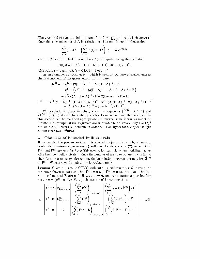
Thus, we need to compute in�nite sum of the formP1j=1 jl �Aj , which convergesince the spectral radius of A is strictly less than one. It can be shown that1Xj=1 jl �Aj = lXi=1 A(l; i) �Ai! � (I�A)�(l+1)where A(l; i) are the Eulerian numbers [10], computed using the recursionA(l; i) = i � A(l � 1; i) + (l � i+ 1) � A(l � 1; i� 1);with A(1; 1) = 1 and A(l; i) = 0 for i < 1 or i > l.As an example, we consider r[1], which is used to compute measures such asthe �rst moment of the queue length. In this case,b[1] = � �(0) � (2(I� A)�1 + A � (I� A)�2) � F� �(1) � �2kL(1) + (3(I�A)�1 +A � (I�A)�2) � F�� r[0] � �A � (I�A)�2 � F+ 2(I�A)�1 �F+ L�c[1] = ��(0)�((I�A)�3+(I�A)�2)�A�F�1T��(1)�(A�(I�A)�3+2(I�A)�2)�F�1T�r[0] � (A � (I�A)�3 + (I�A)�2) � F � 1T :We conclude by observing that, when the sequences fF(j) : j � 1g andfF(j) : j � 1g do not have the geometric form we assume, the treatment inthis section can be modi�ed appropriately. However, some measures might bein�nite. For example, if the sequences are summable but decrease only like 1=jdfor some d > 1, then the moments of order d� 1 or higher for the queue lengthdo not exist (are in�nite).5 The case of bounded bulk arrivalsIf we restrict the process so that it is allowed to jump forward by at most plevels, its in�nitesimal generator Q still has the structure of (2), except thatF(j) and F(j) are zero for j > p (this occurs, for example, when modeling queueswith bounded bulk arrivals). Since the number of matrices on any row is �nite,there is no reason to require any particular relation between the matrices F(j)or F(j). We can then formulate the following lemma.Lemma. Given an ergodic CTMC with in�nitesimal generator Q, having thestructure shown in (2) such that F(j) = 0 and F(j) = 0 for j > p and the �rstn � 1 columns of B are null, B1:n;1:n�1 = 0, and with stationary probabilityvector � = ��(0);�(1);�(2); : : :�, the system of linear equationsx � 266666666664

1T L(0) F1:m;1:n�1 pXj=2 F(j)!1:n;1:n�1 pXj=2(j � 1) � F(j)! � 1T1T B L(1)1:n;1:n�1 pXj=1 F(j)!1:n;1:n�1 pXj=1 j � F(j)! � 1T1T 0 0 pXj=1 F(j) + L!1:n;1:n�1 pXj=1 j � F(j) �B! � 1T377777777775 = [1;0]

admits a unique solution x = [�(0);�(1);�(�)] where �(�) =P1i=2 �(i).Proof: The steps of the proof are exactly the same as those of the theoremintroduced in Sect. 3, hence they are omitted. 2The measure of interest r can also be derived as done in Sect. 4. Using thesame de�nitions for r, �, and r[l], we need to show how to express the vectorsr[l], l = 0; : : : ; k. For brevity's sake, we omit the steps, and simply state that,again, r[k] can be computed recursively by solving the equationr[k] � 240@ pXj=1F(j) + L1A1:n;1:n�1 ������ 0@ pXj=1 j � F(j) �B1A � 1T35 = b[k];where b[k] is computed using �(0), �(1), and r[0] through r[k�1].We stress that we consider the case of �nite bulk arrivals explicitly because,while such type of process could be solved using the version of ETAQA presentedin [2] or the matrix-geometric method [8], by merging every p levels into a largersingle level, the results of this section show how to compute the solution withoutthe corresponding overhead (a factor of p for both execution time and storagein ETAQA, a factor of p3 for execution time and p2 for storage in the matrix-geometric method).6 ETAQA and alternative solution methodsIn this section, we attempt to examine where the extended ETAQA approachwe just introduced lies with respect to alternative solution approaches. We startby saying that M/G/1-type processes have generally received less attention thanGI/M/1-type processes in the literature. This is no doubt due to their greateranalytical complexity and to the lack of such a well-known and successful solutionapproach as the matrix-geometric technique for GI/M/1-type processes. Themain reference we are aware of for the solution of M/G/1-type processes is the\other" book by Neuts, published in 1989, which presents a solution approachwhich we will call \Neuts's algorithm" [9, pages 158-167].Neuts's algorithm is described in terms of a discrete-time Markov chain witha transition probability matrix Q having the same structure as in (2), withL(1) = L (we do not assume this condition in the continuous case because B 6= Bimplies that the diagonal of L(1) might di�er from that of L). The algorithm isbased on the matrix G, whose entry in row i and column i0 represents theprobability that, if the DTMC is in state s(j)i , it will enter level S(j�1) for the�rst time through state s(j�1)i0 . G is stochastic i� the DTMC is recurrent, andthe algorithm assumes that G is irreducible. Several steps are required to obtainthe value of �(0) and �(1).1. Let ~Q = (B+L+P1j=1 F(j)) be the transition probability matrix analogous tothe one de�ned in Sect. 3.1 for the continuous case; compute the column vector� = (L+P1j=1 j �F(j)) � 1T , the probability vector ~� solution of ~� � ~Q = ~�, and� = ~� � �.2. Compute the matrix G minimal solution of G = B+L �G+P1j=1 F(j) �Gj+1

(see [5, 9] for algorithmic issues).3. Compute the probability vector g satisfying g = g �G.4. Compute the matricesX andY solution of X = B+�L+P1j=1 F(j) �Gj��Xand Y =P1j=1 F(j) �Gj�1 + L(0) �Y.5. Compute the stochastic matrices K = L(0) + �P1j=1 F(j) �Gj�1� � X andH = B �Y +P1j=1 F(j) �Gj .6. Compute the probability vectors k and h satisfying k = k �K and h = h �H.7. Compute the column vectors�0 = 24I�B� 1Xj=1 F(j) �Gj35 � hI� ~Q+ (1T � �) � gi�1� 1T + (1� �)�1 �B � 1T ;�00 = 1T + 24 1Xj=1 F(j) �1Xj=1 F(j) �Gj�135 � hI� ~Q+ (1T � �) � gi�1� 1T+(1� �)�1 � 1Xj=1(j � 1) � F(j) � 1T :8. Compute the column vectorsk0 = �00 + 1Xj=1 F(j) �Gj�1 � 24I� L� 1Xj=1F(j) �Gj35 � �0and h0 = �0 + B � (I� L(0))�1 � �00.9. Finally, compute �(0) = (k � k0)�1 � k and �(1) = (h � h0)�1 � h.Once �(0) and �(1) are known, we can then iteratively compute �(j) forj = 2; 3; etc., stopping when the accumulated probability mass is close to one.This can be a numerically intensive step when � is close to one since, in thiscase, the entries of �(j) decrease slowly as j grows.Comparing now ETAQA to Neuts's algorithm, it is only fair to point outimmediately that, while in principle Neuts's algorithm can solve all M/G/1-type processes, our extended ETAQA approach can be applied only when theconnectivity of the states in the CTMC satis�es certain conditions: we essentiallyrequire that B has a single nonzero column (after repartitioning the state space,if required). When ETAQA is applicable, however, it makes sense to investigateits advantages with respect to more general algorithms.The condition we impose on B does simplify Neuts's algorithm considerably,as it implies thatG can be obtained without any computation:Gi;i0 is 1 if i0 = nand 0 otherwise. However, given the complete generality of the matrices L andL(0), the computation of X and Y still requires considerable e�ort and, fromthat point on, the structure of G only reduces the computational complexity ofNeuts's algorithm in the sense that all matrix products containing a factor G on

the right can be performed e�ciently and require only a vector of size n for theirstorage. However, the matrices X, Y, H, and K must be computed and storedin their entirety (at least the last two; X and Y can be actually computedand stored one column at a time), and they are not sparse in general, hencethe computational complexity of is O(m3 + n3) and the storage complexity isO(m2+n2). Furthermore, Neuts's algorithm computes a �nite number of entriesin �, thus any stationary measure obtained from it is, in a sense, approximatebecause of this truncation.Our extended ETAQA method, in addition to its appealing simplicity, allowsus to exploit the sparsity of the blocks de�ning Q, for both execution time andstorage: the matrix M used by ETAQA (or the analogous one for the case ofbounded bulk arrivals) has the same sparsity as the original blocks (the inverses(I� A)�1 and (I�A)�1 require linear computation and storage, since the geo-metric scaling factors A and A are diagonal matrices), and the iterative solutionof the linear system in (4) requires time linear in the number of nonzero entries inM. Furthermore, ETAQA allows instead to e�ciently compute \mathematicallyexact" measures.7 ApplicationsIn this section, we describe two applications that can be solved by the extendedETAQA approach described in Sect. 3. We concentrate on presenting the CTMCsthat models the application of interest and we focus on the form of the repeatingmatrix pattern that allows us to apply our technique.7.1 Multiprocessor schedulingResource allocation in multiprocessor systems has been a favorite research topicfor the performance and operating systems community in recent years. The num-ber of users that attempt to use the system simultaneously, the parallelism ofthe applications and their respective computational and secondary storage needs,and the need to meet the execution deadlines are examples of issues that exac-erbate the di�culty of the resource allocation problem.A popular way to allocate processors among various competing applicationsis by space-sharing the processors: processors are partitioned in disjoint groupsand each application executes in isolation on one of these groups. Space-sharingcan be done in a static, adaptive, or dynamic way. If a job requires a �xednumber of processors for execution, this requires a static space-sharing policy[12]. Adaptive space-sharing policies [1] have been proposed for jobs that cancon�gure themselves to the number of processors allocated by the scheduler atthe beginning of their execution. Dynamic space-sharing policies [6] have beenproposed for jobs that are exible enough to allow the scheduler to reduce oraugment the number of processors allocated to each application in immediateresponse to environment changes. Because of their exibility, dynamic policiescan o�er optimal performance but are the most expensive to implement becausethey reallocate resources while applications are executing.Modeling the behavior of scheduling policies in parallel systems often resultsin CTMCs with matrix-geometric form [13]. Here, we present a CTMC that

models the behavior of a restricted dynamic scheduling policy. A common solu-tion to reducing the processor recon�guration cost in dynamic policies is to limitthe number of reallocations that can occur during the lifetime of a program [1].Fig. 4 illustrates the CTMC of a dynamic scheduling policy that can only reducethe number of processor allocated to an application, and only immediately aftera service completion. We restrict our attention to the system behavior underbursty arrival conditions modeled as bulks of �nite size (see [11] for an analysisof adaptive space-sharing policies under the same assumptions for the arrivalprocess).The system state is described by the number of applications that are wait-ing for service in the queue and the number of applications that are in service.NwMsr denotes that there are N applications in the queue, waiting to be ex-ecuted, and M applications in service, each having a fraction 1r of the totalnumber of processors allocated to it. Thus, the service rate of an application is�r, a function of r. For simplicity, the �gure assumes that the maximum numberof simultaneously executing applications is set to three and that the bulk size isat most four, but any other �nite concurrency level and unbounded bulk sizescan be managed by our approach.A deterministic set of transition rules specify the successor state for each statein the chain. The policy strives to guarantee that all executing applications areallocated an equal number of processors while minimizing the waiting queuelength, but since reallocations occur only at departure times, there are stateswhere there are fewer than three executing applications even when there areapplications waiting in the queue. We further assume that the policy incursno reallocation overhead to illustrate its ideal behavior (this overhead can beaccounted for by reducing the service rates when reallocation occurs).It is easy to observe that our lemma for the bounded bulk arrivals can bereadily applied for the performance analysis of this policy. Since the behaviorof this dynamic scheduling policy under di�erent workloads is outside the scopeof this paper, we do not present numerical results. We point out, however, thatthe average job response time can be easily calculated by �rst computing theaverage queue length as discussed in Sect. 3 and then applying Little's law.7.2 Self-monitoring and self-adjusting serverIn many application domains it is common practice to dynamically add or removeservers so as to dynamically adjust server capacity to incoming workloads [3].The motivation behind such self-adjusting systems is that it is desirable to oper-ate using as few as possible servers when the load is low (and perhaps use the idleservers for other types of work), but at the same time being able to sustain heav-ier workload intensities by dynamically increasing the system capacity throughthe addition of more servers. Examples of such applications include protocolsin communication networks, Internet information query services, and schedulersfor concurrent bandwidth allocation to both multimedia and best-e�ort applica-tions. Here, we concentrate on the behavior of a scheduler that serves applicationsin a time-sharing manner and adjusts its capacity as a function of the arrivalrate intensity.

1

2µ3 3µ3 3µ3 3µ3

22µ 2

3µ

µ2

µ1 µ

2µ

µ1

2µ

1

2µ22

µ1µ

λβ

1w1s1 2w1s1 3w1s1 4w1s1--λα

λγ

λδ

λα λα λα λα

λβ

λγ

λδ

λβ λβ

λγ

λβ

0w1s 0w2s 0w3s 1w3s3 2w3s3

λβλβλβλβ

0w2s 1w2s2 2w2s2 3w2s2

λα λα λα λα

λβ λβ λβ λβ

λγ λγ λγ

λγλγλγ

λδ λδ

λδλδ

. . .

. . .

. . .

λδ

0w1s1

0w1s2

3 3 3

2

Fig. 4. The CTMC that models a dynamic multiprocessor scheduling policy.A generic CTMC that describes the behavior of such systems is illustratedin Fig. 5. The system state de�nes the number of applications in the system andthe current service level. We assume that the server can operate at four levels,a, b, c, and d. Requests to the system may come from two sources. The �rst oneis Poisson with parameter �, while the second one is Poisson with parameter� but may be of arbitrary bulk size. The bulk size is governed by a geometricdistribution with parameter 1� � (for the sake of clarity, Fig. 5 shows the bulkarrivals only for service level a).The service station increases its capacity gradually, according to the currentworkload. The time to add a new server is exponentially distributed with param-eter �; this may occur during the service levels a, b, and c. We further assumethat the reduction of server capacity is instantaneous and occurs only when thesystem empties completely (modeling an actual delay for taking servers o�inecan be easily accommodated, since it just increases the set of states S(0)).It is easy to verify that our extended version of ETAQA can be readily appliedafter repartitioning the state space as shown by the grayed-out areas in Fig. 5.8 Conclusions and future workIn this paper we presented an extension of the ETAQA approach to M/G/1-typeprocesses. Our exposition focuses on the description of the extended ETAQAmethodology and its application to e�ciently compute the exact probabilitiesof the boundary states of the process and the aggregate probability distribu-tion of the states in each of the equivalence classes corresponding to a speci�cpartitioning of the remaining in�nite portion of the state space. Although themethod does not compute the probability distribution of all states, it still pro-vides enough information for the \mathematically exact" computation of a widevariety of Markov reward functions.

µ2

µ3

µ4 µ 4 µ4

µ

4

1µ

µ

µ

4

µ 1µ

2µ 2µ 2

1

2µ

3µ 3µ

1

µ 3µ

µ

2(1−ρ) κρ2(1−ρ) κρ2(1−ρ) κρ2(1−ρ)

κρ3(1−ρ)κρ3(1−ρ)

3

3(1−ρ)κρ3(1−ρ)

κρ4(1−ρ) κρ4(1−ρ)κρ4

κρ

κρ

(1−ρ)

1µ1a 2a 3a 4a 5a

1b 2b 3b 4b 5b

1c 2c 3c 4c 5c

0a

1d 2d 3d 4d 5d

λ

λ

λλ

λ

λλ

λ

λλ

λ

λ

λ+κ(1−ρ) λ+κ(1−ρ) λ+κ(1−ρ) λ+κ(1−ρ)

κρ(1−ρ) κρ(1−ρ) κρ(1−ρ) κρ(1−ρ) κρ(1−ρ)

... ... ...

...

...

...

...

ν ν ν ν ν

ν

νν

νννν

νν

...

λ+κ(1−ρ)

Fig. 5. The CTMC that models a self-monitoring and self-adjusting server.We must emphasize that our treatment does not apply to all M/G/1-typeprocesses. The necessary condition that must be satis�ed is that all transitionsfrom one level to the previous one are directed to a single state (but no restric-tion is placed on transitions within a level or toward higher levels). When thiscondition is satis�ed, the solution is derived by solving a system of m+ 2n lin-ear equations and provides signi�cant savings over standard algorithms for thesolution of general M/G/1-type processes. Although the condition on B is indis-putably restrictive, we present a set of applications from the computer systems�eld where extended ETAQA readily applies.In the future, we expect to release a software tool that e�ciently implementsthe extended ETAQA. Implementation of the tool is currently underway. Wealso intend to explore possibilities to extend the methodology to a wider class ofM/G/1-type processes than those presented in this paper. To this end, the utilityof approximation methods based on the extended ETAQA will be examined.AcknowledgmentsWe would like to thank our colleague Prof. Paul Stockmeyer for furnishing uswith the expression for the sumP1j=1 jl �Aj , and its relation to Euler numbers.There just isn't a substitute for having a good mathematician in the house! Wealso would like to thank the anonymous referees for their insightful suggestions.References1. S.-H. Chiang, R. Mansharamani, and M. Vernon. Use of application characteristicsand limited preemption for run-to-completion parallel processor scheduling policies.

In Proceedings of the 1994 Sigmetrics Conference on Measurement and Modelingof Computer Systems, pages 33{44, May 1994.2. G. Ciardo and E. Smirni. ETAQA: An E�cient Technique for the Analysis ofQBD-processes by Aggregation. Submitted for publication.3. L. Golubchik and J. C. Lui. Bounding of performance measures of a threashold-based queueing system with hysteresis. In Proceedings of the 1997 ACM SIG-METRICS International Conference on Measurement and Modeling of ComputerSystems, pages 147{156, June 1997.4. G. Latouche. Algorithms for in�nite Markov chains with repeating columns.In C. Meyer and R. J. Plemmons, editors, Linear Algebra, Markov Chains, andQueueing Models, volume 48 of IMA Volumes in Mathematics and its Applica-tions, pages 231{265. Springer-Verlag, 1993.5. G. Latouche and G. W. Stewart. Numerical methods for M/G/1 type queues. InW. J. Stewart, editor, Computations with Markov Chains, pages 571{581. Kluwer,Boston, MA, 1995.6. C. McCann, R. Vaswani, and J. Zahorjan. A dynamic processor allocation pol-icy for multiprogrammed shared memory multiprocessors. ACM Transactions onComputer Systems, 11(2):146{178, 1993.7. R. Nelson. Probability, Stochastic Processes, and Queueing Theory. Springer-Verlag, 1995.8. M. F. Neuts. Matrix-geometric solutions in stochastic models. Johns HopkinsUniversity Press, Baltimore, MD, 1981.9. M. F. Neuts. Structured stochastic matrices of M/G/1 type and their applications.Marcel Dekker, New York, NY, 1989.10. J. Riordan. An Introduction to Combinatorial Analysis. Wiley Series in Probabil-ity and Mathematical Statistics. John Wiley & Sons, 1958.11. E. Rosti, E. Smirni, G. Serazzi, L. Dowdy, and K. Sevcik. On processor savingscheduling policies for multiprocessor systems. IEEE Trans. Comp., 47(2):178{189, Feb. 1998.12. E. Smirni, E. Rosti, L. Dowdy, and G. Serazzi. A methodology for the evaluationof multiprocessor non-preemptive allocation policies. Journal of Systems Architec-ture, 44:703{721, 1998.13. M. Squillante, F. Wang, and M. Papaefthymiou. Stochastic analysis of gangscheduling in parallel and distributed systems. Perf. Eval., 27/28:273{296, 1996.14. G. W. Stewart. On the solution of block hessenberg systems. Numerical LinearAlgebra with Applications, 2:287{296, 1995.

This article was processed using the LATEX macro package with LLNCS style