An Adaptive Harmonic Balance Method for predicting the non linear dynamicresponses of mechanical systems - Application to bolted structures

V. Jaumouillea,b, J-J. Sinoua and B. Petitjeanb

a Laboratoire de Tribologie et Dynamique des Systemes UMR-CNRS 5513, Ecole Centrale de Lyon,36 avenue Guy de Collongue,69134 Ecully Cedex, France.

b EADS Innovation Works, 12 rue Pasteur, 92150 Suresnes, France.

Keywords : Harmonic balance method, bolted joint, nonlinear model, continuation, condensation.

Abstract

Aeronautical structures are commonly assembled with bolted joints in which friction phenomena, incombination with slapping in the joint, provide damping on the dynamic behaviour. Some models,mostly non linear, have consequently been developed and theharmonic balance method (HBM) isadapted to compute non linear response functions in the frequency domain. The basic idea is to de-velop the response as Fourier series and to solve equations linking Fourier coefficients. One specificHBM feature is that response accuracy improves as the numberof harmonics increases, at the expenseof larger computational time. Thus this paper presents an original adaptive HBM which adjusts thenumber of retained harmonics for a given precision and for each frequency value. The new proposedalgorithm is based on the observation of the relative variation of an approximate strain energy fortwo consecutive numbers of harmonics. The developed criterion takes the advantage of being cal-culated from Fourier coefficients avoiding time integration and is also expressed in a condensationcase.However, the convergence of the strain energy has to be smooth on tested harmonics and thisconstitutes a limitation of the method.Condensation and continuation methods are used to acceleratecalculation. An application case is selected to illustratethe efficiency of the method and is composedof an asymmetrical two cantilever beam system linked by a bolted joint represented by a nonlinearLuGre model. The practice of adaptive HBM shows that, for a given value of the criterion, the num-ber of harmonics increases on resonances indicating that non linear effects are predominant. For eachfrequency value, convergence of approximate strain energyis observed. Emergence of third and fifthharmonics is noticed near resonances both on vibratory responses and on approximate strain energy.Parametric studies are carried out by varying the excitation force amplitude and the threshold valueof the adaptive algorithm. Maximal amplitudes of vibrationand frequency response functions areplotted for three different points of the structure. Non linear effects become more predominant forhigher force amplitudes and consequently the number of retained harmonics is increased.

1

hal-0

0625

097,

ver

sion

1 -

25 S

ep 2

012

Author manuscript, published in "Journal of Sound and Vibration 329 (2010) 4048-4067" DOI : 10.1016/j.jsv.2010.04.008

1 Introduction

The dynamics of mechanical structures is strongly influenced by the presence of riveted or boltedjoints in the structure. Indeed structural joints generateenergy dissipation through the complex rela-tive motion between two contacting surfaces, commonly referred as frictional slip. Additionally forhigher level of excitation, slapping may be encountered. Frictional slip may be analyzed by consider-ing an interface behaviour divided in two cases: micro-slipwhere part of the interface is slipping; andmacro-slip where all the interface slips. Then the frictional energy dissipation observed in the slipzone is responsible for the vibration damping attributed tojoints [1]. Gaul et al. [2] showed that thisdamping may be larger than material damping and Beards [3] mentioned that up to90% of the totalsystem damping might be provided by the joints. Thorough reviews about damping in joints may befound in the works of Ungar [4], Gaul et al. [2] and more recently Ibrahim et al. [5].

A better prediction of this damping effect is now an important objective for many aeronauticalcompanies and various complex industrial structures incorporating bolted joints have been investi-gated [6–9]. Crocombe et al. [7] established a relationshipbetween energy dissipated in a joint andthe transverse excitation force using a 3D FE model of a bolted joint and then used this relationshipin conjunction with the simulation of a FE model of a satellite to estimate the energy dissipated in thejoints. In the work of Caignot [9], a micro scale model of bolted joints quantifies in a first step thejoint dissipation and an equivalent modal damping is deduced in a second step to perform dynamicanalysis of the whole studied structure.

These approaches perform a complex contact analysis givingan insight into the distribution andamount of friction on the interfaces but neglect non linear effects in the global dynamic behaviourof the assembled bolted structure. They need detailed models, often impractical for dynamic analysesof large structures. Hence constitutive models which use a number of degrees of freedom adapted tostructural dynamics may be a suitable and computationally efficient alternative. These models canbe divided into lumped models and thin layer element theories [10]. In lumped models, the effect ofjoint is considered to be concentrated at a single point and the joint model has no dimension. Severalmodels have been proposed: the Valanis model [11], the elasto-slip model [2], the LuGre model [2],the Iwan model [1], the Bouc-Wen model [12], models with Jenkins elements [12] and models inte-grating a cubic stiffness [13]. The second category, based on thin layer elements, is represented asan element with physical dimensions and specific force-displacement relation. Ahmadian et al. [10]developed a generic joint element based on a thin layer element approach and Song et al. [14] devel-oped an adjusted Iwan beam element incorporating an Iwan model to simulate the dynamics of beamstructures.

Most of these models are non linear and require specific methods to compute non linear frequencyresponse functions. In order to compute responses to forcedexcitation, one of the first methods istime integration. Oldfield et al. [12] applied time integration on a bolted structure to simulate hystere-sis loops using a Jenkins element model and a Bouc-Wen model.Other applications on a two beamsystem were encountered in the works of Gaul et al. [11] and Miller et al. [15]. Time integrationmay be inefficient on lightly damped structures because the transient response may take hundreds offorcing periods at the expense of calculation time and disc storage size. Other alternatives like pertur-bation methods and the Krylov and Bogoliubov method remain limited to a few degrees of freedom.

2

hal-0

0625

097,

ver

sion

1 -

25 S

ep 2

012

Heller et al. [16] applied the Krylov-Bogoliubov method on anon linear system in order to determineequivalent modal parameters and not to compute periodic responses.

In the frequency domain, the harmonic balance method (HBM) is able to compute periodic responsesof non linear systems. The basics are to develop the unknown response as a truncated Fourier seriesand to solve equations linking Fourier coefficients. First mechanical applications can be encounteredin the works of Pierre et al. [17] on a single degree of freedomdry friction damped system and Ferriet al. [18] on a beam incorporating dry friction. Then a further development of the HBM, named Al-ternating Frequency Time Domain Method [19], numerically evaluates the Fourier transform of localnonlinearities of the model and does not require to analytically describe non linear terms. More re-cently, other approaches have been proposed, notably the Constrained Harmonic Balance Method [20]which computes solutions for periodic autonomous systems.For dynamic analyses of bolted joints,Gaul et al. [2] used harmonic balance method for the calculation of an equivalent stiffness and vis-cous damping in an elasto-slip model. Ren et al. [21] proposed a general technique for identifyingthe dynamic properties of nonlinear joints using dynamic test data and used multi-harmonic balancemethod to identify parameters for a friction joint. These two developments compute hysteresis loopsand not periodic responses. The work of Ahmadian et al. [10] developed a non linear generic ele-ment formulation for bolted joints and used a cubic non linear stiffness to represent softening nonlinear effects. Then frequency response curves of the system are calculated with the HBM allowingto include these curves in a minimization procedure in orderto identify parameters of the joint. Onlyprime harmonics were considered due to experimental considerations.

One specific HBM feature is that response accuracy improves as the number of harmonics in the trun-cated Fourier series increases, at the expense of larger computational time. Therefore only harmonicswhich lead to a significant contribution on dynamic responsemust be taken into account for a givenprecision, and their number can strongly vary on a frequencyinterval.This key point has been highlighted for bolted joint dynamics by Ouyang et al. [22] who studied an ex-perimental two beam bolted system excited at resonance. By increasing importance of friction in thejoints (through an increase of the excitation amplitude), measured hysteresis loops became distortedand superharmonics appeared in the frequency spectra of theresponses, showing the importance ofconsidering higher order terms in the Fourier development of the response. Only odd harmonics werepresent suggesting the possibility to use a cubic stiffnessin the bolted joint model [10,13] and to onlyconsider odd harmonics in the harmonic balance method, usual practice for dry friction system [17].

Even though, up to now, no theoretical tool can determine which harmonics are predominant for anon linear system. The present study pursues this investigation by developing a criterion allowingto limit the number of retained harmonics. An approximate strain energy with Fourier coefficientsis calculated and its saturation is monitored. This new criterion, based on Fourier coefficients, doesnot require time integration and may be easily estimated. Inorder to illustrate the efficiency of themethod on a non linear mechanical system, an asymmetrical two cantilever beam system linked bya bolted joint is modelled as application case. The joint model was inspired by the Adjusted IwanBeam Element (AIBE) developed by Song [14]. However, a LuGremodel was preferred to an Iwanmodel present in the work of Song for implementation simplicity. Moreover, formulation of HBMhas consequently been adapted to integrate LuGre model internal variables. Analysis of frequencyresponse functions and detailed monitoring of criterion evolution help to assess the validity of this ap-

3

hal-0

0625

097,

ver

sion

1 -

25 S

ep 2

012

proach. In order to accelerate calculation, a condensationprocedure on non linear degrees of freedomis performed by reformulating the HBM equations. Furthermore, criterion has been expressed in thiscase and compared with case without condensation.

This paper is divided into three main sections. The first one deals with the HBM formulation, detailscondensation and criterion expression. Secondly, the studied system is presented and HBM adaptationto LuGre model is detailed. Finally, result analyses highlight the effect of the harmonic selectionprocess on frequency response functions and on the number ofretained harmonics, and a parametricstudy on the influence of the excitation force is discussed.

2 HBM Formulation

2.1 General Formulation

We consider a discrete mechanical system withnddl degrees of freedoms (dofs) described with itsnddl × nddl mass matrixM, stiffness matrixK and damping matrixD. An external periodic forceFL(Ω, t) is applied to the system with an angular frequencyΩ. System non linearities are consideredas a non linear forceFNL(X, X,Ω, t) which depends on degrees of freedom displacementsX, veloc-ities X, angular frequencyΩ and timet. The global forceF (X, X,Ω, t) applied on the system maybe divided in two parts, the linear external forceFL(Ω, t) and the non linear forceFNL(X, X,Ω, t).The governing equation of motion may be written as:

MX +DX +KX = F (X, X,Ω, t) = FL(Ω, t) + FNL(X, X,Ω, t) (1)

First, we assume a periodic responseX(t), which allows to develop the solution as a Fourier series.This development is theoretically infinite so a truncation in the following form is needed:

X(t) = B0 +m∑

k=1

(

Ak sin(k

νΩt) +Bk cos(

k

νΩt)

)

X(t) =

[

I sin(Ω

νt)I cos(

Ω

νt)I . . . sin(

k

νΩt)I cos(

k

νΩt)I . . .

]

[B0 A1 B1 . . . Ak Bk . . .]T

X(t) = T(t)Z (2)

whereI is thenddl×nddl identity matrix,Z = [B0 A1 B1 . . . Ak Bk . . .]T is the(2m+1)nddl×1vector containing Fourier coefficients,m is the number of harmonics retained for the truncation,ν isan integer used to represent possible subharmonics, andT(t) = [I sin(Ω

νt)I cos(Ω

νt)I . . . sin(k

νΩt)I

cos(kνΩt)I . . .] is thenddl × (2m+ 1)nddl matrix containing trigonometric functions.

The same work is then accomplished for the global forceF :

F (X, X,Ω, t) = C0 +m∑

k=1

(

Sk sin(k

νΩt) + Ck cos(

k

νΩt)

)

F (X, X,Ω, t) = T(t) [C0 S1 C1 . . . Sk Ck . . .]T

F (X, X,Ω, t) = T(t)b (3)

4

hal-0

0625

097,

ver

sion

1 -

25 S

ep 2

012

In order to compute velocities and accelerations, we define afrequential derivative operator:

∇ = diag(0nddl×nddl,∇1, . . . ,∇m) with ∇k =k

νΩ

[

0 −I

I 0

]

(4)

Thus we may write:

X(t) = T(t)∇Z

X(t) = T(t)∇2Z (5)

By replacing Eqn. (2) and Eqn. (5) into Eqn. (1), one obtains:

MT(t)∇2Z +DT(t)∇Z +KT(t)Z = T(t)b (6)

Considering that for anddl × nddl matrixW and a(2m+ 1)nddl× 1 vectorY :

WT(t)Y = T(t)NWY (7)

with NW = diag(W,W, . . .) (2m+ 1)nddl×(2m+ 1)nddl

.

Equation (6) becomes:

T(t)NM∇2Z +T(t)ND∇Z +T(t)NKZ = T(t)b

T(t)(

NM∇2 +ND∇+NK

)

Z = T(t)b (8)

Time dependency may be suppressed and a frequency algebraicequation linking Fourier coefficientmay be obtained using a Galerkin method which is a projectionof the equation on trigonometricfunctions. Indeed these trigonometric functions define a scalar product:

< f, g >=1

T

∫ T

0f(t)g(t)dt (9)

Thus we may write:

1

T

∫ T

0

TT(t)T(t)dt =

1

2

2I 0

I

I

0. . .

= L (2m+ 1)nddl×(2m+ 1)nddl

(10)

Applying this scalar product on Eqn. (8) leads to:

1

T

∫ T

0

TTT

(

NM∇2 +ND∇+NK

)

Z dt =1

T

∫ T

0

TTT b dt

L

(

NM∇2 +ND∇+NK

)

Z = L b (11)

L is a diagonal matrix so Eqn. (11) may be simplified into a(2m+ 1) ∗ nddl equation system:

AZ = b with A = NM∇2 +ND∇+NK (12)

5

hal-0

0625

097,

ver

sion

1 -

25 S

ep 2

012

A may be expressed in a simpler manner:

A =

K

K−(Ων

)2M −Ω

νD

ΩνD K−

(Ων

)2M

. . .

K−(kνΩ)2

M −kνΩD

kνΩD K−

(kνΩ)2

M

. . .

(13)

This system is equivalent of finding zeros of a functionH : IR(2m+1)×nddl → IR(2∗m+1)×nddl:

H(Z) = A(Ω)Z − b(Z,Ω) (14)

We note thatb is dependent onZ andΩ becauseb corresponds to the Fourier coefficients ofF (X, X,Ω, t).In the case where no analytical expression may be written betweenb andZ, an evaluation of the ap-proximate temporal termsX(t) andX(t) is carried out from an initial valueZ = T [B0A1B1 . . . AmBm]:

ZFFT=⇒ X(t) = B0 +

m∑

k=1

(Ak sin(k

νΩt) +Bk cos(

k

νΩt)) (15)

It also allows to evaluate temporarily the non linear termFNL(X, X,Ω, t) and then to deduce Fouriercoefficients by aFFT procedure:

FNL(X, X,Ω, t)FFT=⇒ bNL(Z,Ω) =

T [CNL0 SNL

1 CNL1 . . . SNL

m CNLm ] (16)

2.2 Condensation

An additional step can reduce the number of equations to solve. It consists in expressing Fouriercoefficients of dofs on which no nonlinearity is applied (called linear dofs) functions of Fourier coef-ficients of remaining dofs (called non linear dofs) and of Fourier coefficients of linear and non linearforces:First, dofs are reorganized intop linear dofs andq non linear dofs using a boolean transition matrixP:

X = P

[

Xp

Xq

]

=[

Pp Pq

][

Xp

Xq

]

(17)

wherePp is anddl×p matrix containing the first p columns ofP,Pp contains the last q columns ofP.

Using the same decomposition for Fourier coefficients,Zp = [B0p A1p B1p . . . Amp Bmp]T (idem for

Zq), the following result is obtained:

Z =[

NPpNPq

][

Zp

Zq

]

(18)

6

hal-0

0625

097,

ver

sion

1 -

25 S

ep 2

012

Note thatNPpandNPq

are respectively(2m+ 1)nddl× (2m+ 1)p and(2m+ 1)nddl× (2m+ 1)qmatrices.NP andP are both boolean matrices too andT

NPNP = I.

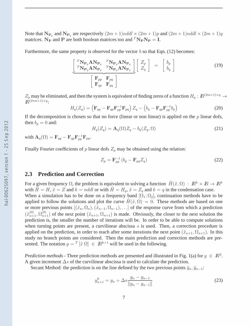
Furthermore, the same property is observed for the vectorb so that Eqn. (12) becomes:[

TNPp

ANPp

TNPp

ANPq

TNPq

ANPp

TNPq

ANPq

]

︸ ︷︷ ︸[

Fpp Fpq

Fqp Fqq

]

[

Zp

Zq

]

=

[

bpbq

]

(19)

Zp may be eliminated, and then the system is equivalent of finding zeros of a functionHq : IR(2m+1)×q →

IR(2∗m+1)×q :Hq(Zq) =

(

Fqq − FqpF−1pp Fpq

)

Zq −(

bq − FqpF−1pp bp

)

(20)

If the decomposition is chosen so that no force (linear or nonlinear) is applied on thep linear dofs,thenbp = 0 and:

Hq(Zq) = Aq(Ω)Zq − bq(Zq,Ω) (21)

with Aq(Ω) = Fqq − FqpF−1pp Fpq.

Finally Fourier coefficients ofp linear dofsZp may be obtained using the relation:

Zp = F−1pp (bp − FpqZq) (22)

2.3 Prediction and Correction

For a given frequencyΩ, the problem is equivalent to solving a functionH(x,Ω) : IRk × IR → IRk

with H = H, x = Z andk = nddl or with H = Hq, x = Zq andk = q in the condensation case.When a simulation has to be done on a frequency band[Ω1; Ω2], continuation methods have to beapplied to follow the solutions and plot the curveH(x,Ω) = 0. These methods are based on oneor more previous points[(xn,Ωn), (xn−1,Ωn−1), . . .] of the response curve from which a prediction(x

(0)n+1,Ω

(0)n+1) of the next point(xn+1,Ωn+1) is made. Obviously, the closer to the next solution the

prediction is, the smaller the number of iterations will be.In order to be able to compute solutionswhen turning points are present, a curvilinear abscissas is used. Then, a correction procedure isapplied on the prediction, in order to reach after some iterations the next point(xn+1,Ωn+1). In thisstudy no branch points are considered. Then the main prediction and correction methods are pre-sented. The notationy = T [x Ω] ∈ IRk+1 will be used in the following.

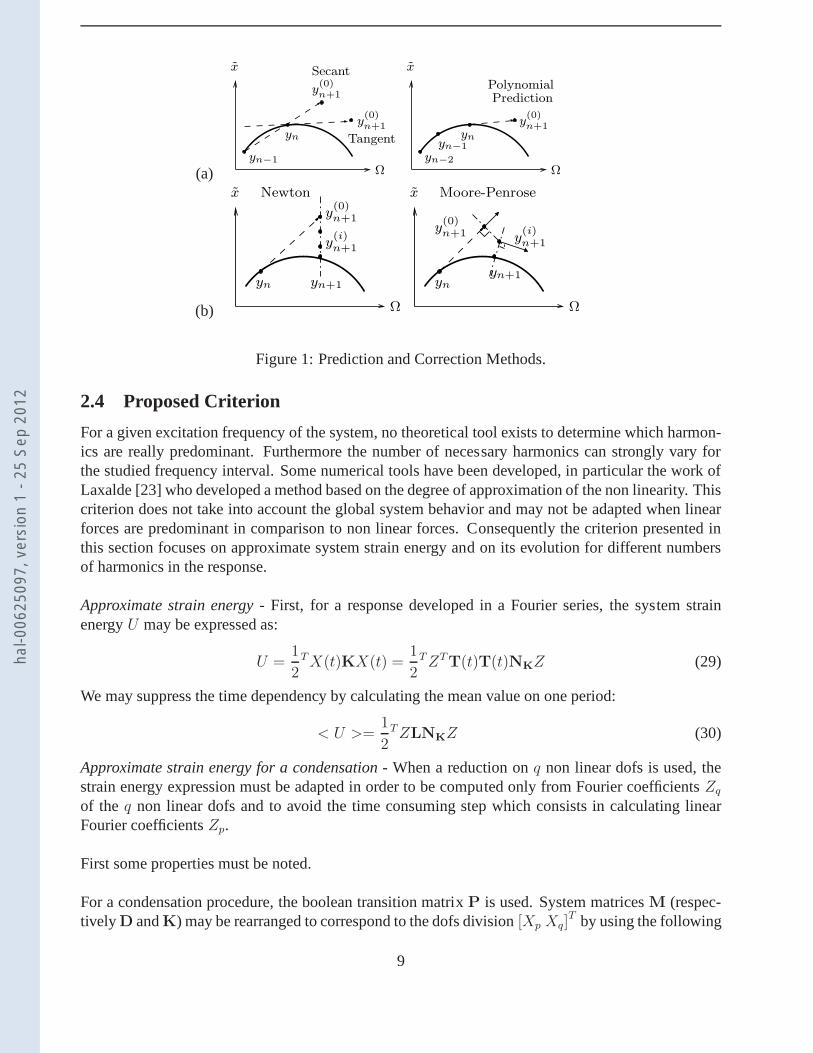
Prediction methods- Three prediction methods are presented and illustrated inFig. 1(a) fory ∈ IR2.A given increment∆s of the curvilinear abscissa is used to calculate the prediction.

Secant Method: the prediction is on the line defined by the twoprevious pointsyn, yn−1:

y0n+1 = yn +∆syn − yn−1

‖yn − yn−1‖(23)

7

hal-0

0625

097,

ver

sion

1 -

25 S

ep 2

012

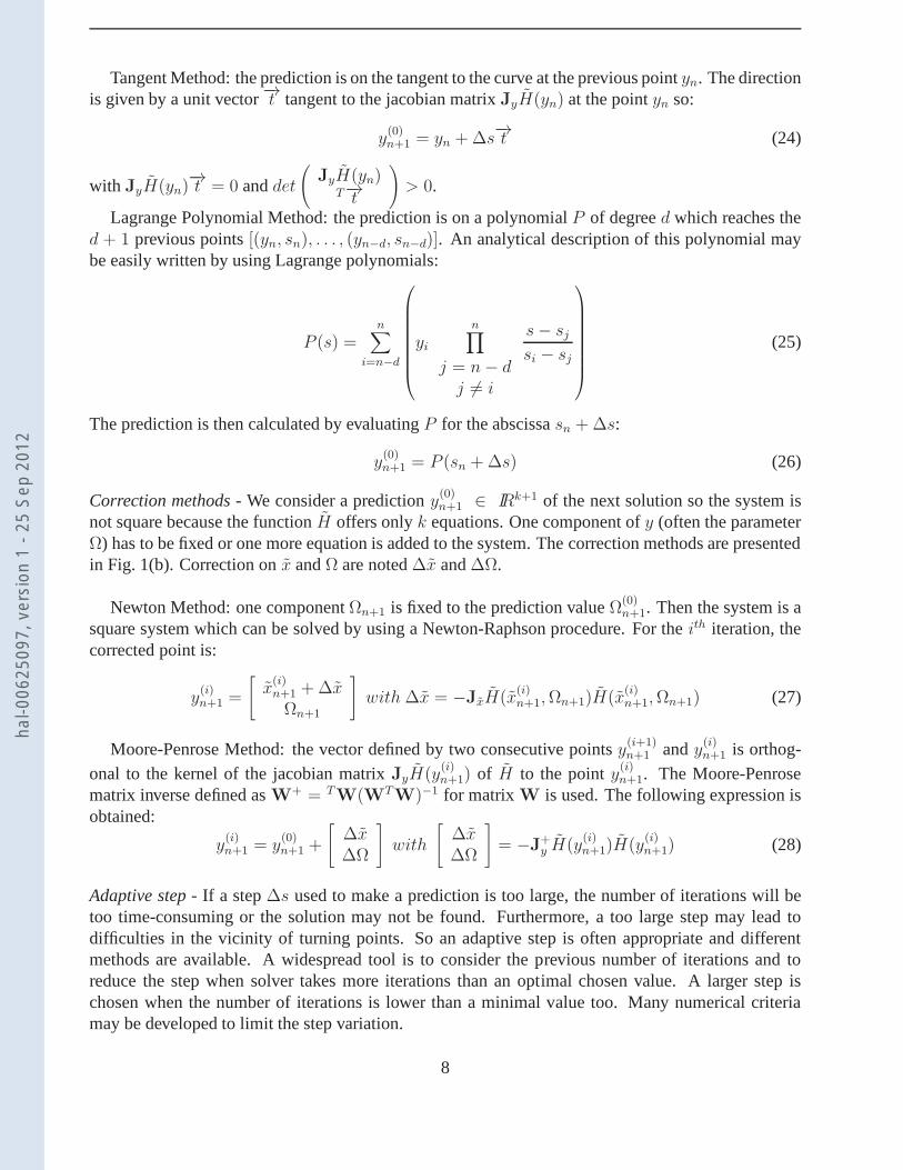
Tangent Method: the prediction is on the tangent to the curveat the previous pointyn. The directionis given by a unit vector−→t tangent to the jacobian matrixJyH(yn) at the pointyn so:

y(0)n+1 = yn +∆s

−→t (24)

with JyH(yn)−→t = 0 anddet

(

JyH(yn)T−→t

)

> 0.

Lagrange Polynomial Method: the prediction is on a polynomialP of degreed which reaches thed + 1 previous points[(yn, sn), . . . , (yn−d, sn−d)]. An analytical description of this polynomial maybe easily written by using Lagrange polynomials:

P (s) =n∑

i=n−d

yin∏

j = n− dj 6= i

s− sjsi − sj

(25)

The prediction is then calculated by evaluatingP for the abscissasn +∆s:

y(0)n+1 = P (sn +∆s) (26)

Correction methods- We consider a predictiony(0)n+1 ∈ IRk+1 of the next solution so the system isnot square because the functionH offers onlyk equations. One component ofy (often the parameterΩ) has to be fixed or one more equation is added to the system. Thecorrection methods are presentedin Fig. 1(b). Correction onx andΩ are noted∆x and∆Ω.

Newton Method: one componentΩn+1 is fixed to the prediction valueΩ(0)n+1. Then the system is a

square system which can be solved by using a Newton-Raphson procedure. For theith iteration, thecorrected point is:

y(i)n+1 =

[

x(i)n+1 +∆xΩn+1

]

with ∆x = −JxH(x(i)n+1,Ωn+1)H(x

(i)n+1,Ωn+1) (27)

Moore-Penrose Method: the vector defined by two consecutivepointsy(i+1)n+1 andy(i)n+1 is orthog-

onal to the kernel of the jacobian matrixJyH(y(i)n+1) of H to the pointy(i)n+1. The Moore-Penrose

matrix inverse defined asW+ = TW(WT

W)−1 for matrixW is used. The following expression isobtained:

y(i)n+1 = y

(0)n+1 +

[

∆x∆Ω

]

with

[

∆x∆Ω

]

= −J+y H(y

(i)n+1)H(y

(i)n+1) (28)

Adaptive step- If a step∆s used to make a prediction is too large, the number of iterations will betoo time-consuming or the solution may not be found. Furthermore, a too large step may lead todifficulties in the vicinity of turning points. So an adaptive step is often appropriate and differentmethods are available. A widespread tool is to consider the previous number of iterations and toreduce the step when solver takes more iterations than an optimal chosen value. A larger step ischosen when the number of iterations is lower than a minimal value too. Many numerical criteriamay be developed to limit the step variation.

8

hal-0

0625

097,

ver

sion

1 -

25 S

ep 2

012

(a)

x

yn

y(0)n+1

y(0)n+1

Secant

Ωyn−1

Tangent

x

yn

Ωyn−2

y(0)n+1

yn−1

PolynomialPrediction

(b)

x

y(0)n+1

yn yn+1

y(i)n+1

Newton

Ω

x

Ω

yn

Moore-Penrose

yn+1

y(0)n+1

y(i)n+1

Figure 1: Prediction and Correction Methods.

2.4 Proposed Criterion

For a given excitation frequency of the system, no theoretical tool exists to determine which harmon-ics are really predominant. Furthermore the number of necessary harmonics can strongly vary forthe studied frequency interval. Some numerical tools have been developed, in particular the work ofLaxalde [23] who developed a method based on the degree of approximation of the non linearity. Thiscriterion does not take into account the global system behavior and may not be adapted when linearforces are predominant in comparison to non linear forces. Consequently the criterion presented inthis section focuses on approximate system strain energy and on its evolution for different numbersof harmonics in the response.

Approximate strain energy- First, for a response developed in a Fourier series, the system strainenergyU may be expressed as:

U =1

2TX(t)KX(t) =

1

2TZT

T(t)T(t)NKZ (29)

We may suppress the time dependency by calculating the mean value on one period:

< U >=1

2TZLNKZ (30)

Approximate strain energy for a condensation- When a reduction onq non linear dofs is used, thestrain energy expression must be adapted in order to be computed only from Fourier coefficientsZq

of the q non linear dofs and to avoid the time consuming step which consists in calculating linearFourier coefficientsZp.

First some properties must be noted.

For a condensation procedure, the boolean transition matrix P is used. System matricesM (respec-tivelyD andK) may be rearranged to correspond to the dofs division[Xp Xq]

T by using the following

9

hal-0

0625

097,

ver

sion

1 -

25 S

ep 2

012

Initialization and Prediction : m = 0 , < U >= 0, (x(0)n+1, Ω

(0)n+1)

m = m + 1

HBM CalculationSolution for m harmonics : (xn+1, Ωn+1)m

Evaluation of < Um >= T xn+1Kxn+1

Evaluation of criterion ǫ = <Um>−<Um−1>

<Um>no

Test : ǫ < ǫthreshold

yes

Solution : (xn+1, Ωn+1) = (xn+1, Ωn+1)m−1

with x =

Z

or

Zq

and K =

K

or

Kqq −TKqpK

−1pp Kpq

.

Figure 2: Algorithm for criterionǫ.

conversionM = TPMP (respectivelyD andK). Similarly toF in Eqn. (19),M may be divided in

four blocks:Mkl =

TPkMPl with (k, l) ∈ p, q (31)

Furthermore, for ar × s matrixW and as× t matrixV, NWNV = NWV andTNW = NTW.

Then, if the matrixdiag(0k×k,∇1, . . . ,∇m) with identity matrix asIk×k is named∇k, the followingformula may be obtained:

∇NPk= NPk

∇k with k ∈ p, q (32)

Finally, the matrixLk is a(2m+1)k× (2m+1)k matrix with identity matrix asIk×k andk ∈ p, q.

For the computation of criterion in the reduction case, Eqn.(30) becomes:

< U > =1

2TZLNKZ

< U > =1

2

[TZp

TZq

][

TNPp

TNPq

]

LNK

[

NPpNPq

][

Zp

Zq

]

< U > =1

2

[TZp

TZq

][

Lp 0

0 Lq

] [

NPpKPpNPpKPq

NPqKPpNPqKPq

] [

Zp

Zq

]

< U > =1

2(TZpLpNKpp

Zp +TZpLpNKpq

Zq

+TZqLqNKqpZp +

TZqLqNKqqZq) (33)

10

hal-0

0625

097,

ver

sion

1 -

25 S

ep 2

012

Then, a more explicit form of matrixF (Eqn. (19)) must be established:

Fkl =TNPk

ANPl(34)

Introducing the expression of matrixA of Eqn. (12) leads to:

Fkl = TNPk

(

NM∇2 +ND∇+NK

)

NPl

Fkl = NMkl∇2

l +NDkl∇l +NKkl

(35)

with (k, l) ∈ p, q. For simplicity, linear and non linear Fourier coefficientsare supposed to belinked in a static case (Ω = 0) so that∇l = 0l×l.By using this assumption in Eqn. (22),Zp may be expressed as:

Zp = N−1Kpp

(

bp −NKpqZq

)

(36)

If the decomposition is chosen so that no force (linear or nonlinear) is applied on thep linear dofs,thenbp = 0 and:

Zp = −N−1Kpp

NKpqZq (37)

By replacing Eqn. (37) into Eqn. (33):

< U > =1

2(TZq

TN

Kpq

TN

K−1ppLpNKpp

NK

−1ppN

KpqZq

+TZqTN

Kpq

TN

K−1ppLpNKpq

Zq

+TZqLqNKqpN

K−1ppN

KpqZq

+TZqLqNKqqZq)

< U > =1

2TZqLqNKqq−

T KqpK−1pp Kpq

Zq (38)

This equation is very similar to Eqn. (30) obtained for the non reduced case. MatrixKqq−TKqpK

−1pp Kpq

acts as reduced stiffness matrix on theq non linear dofs.

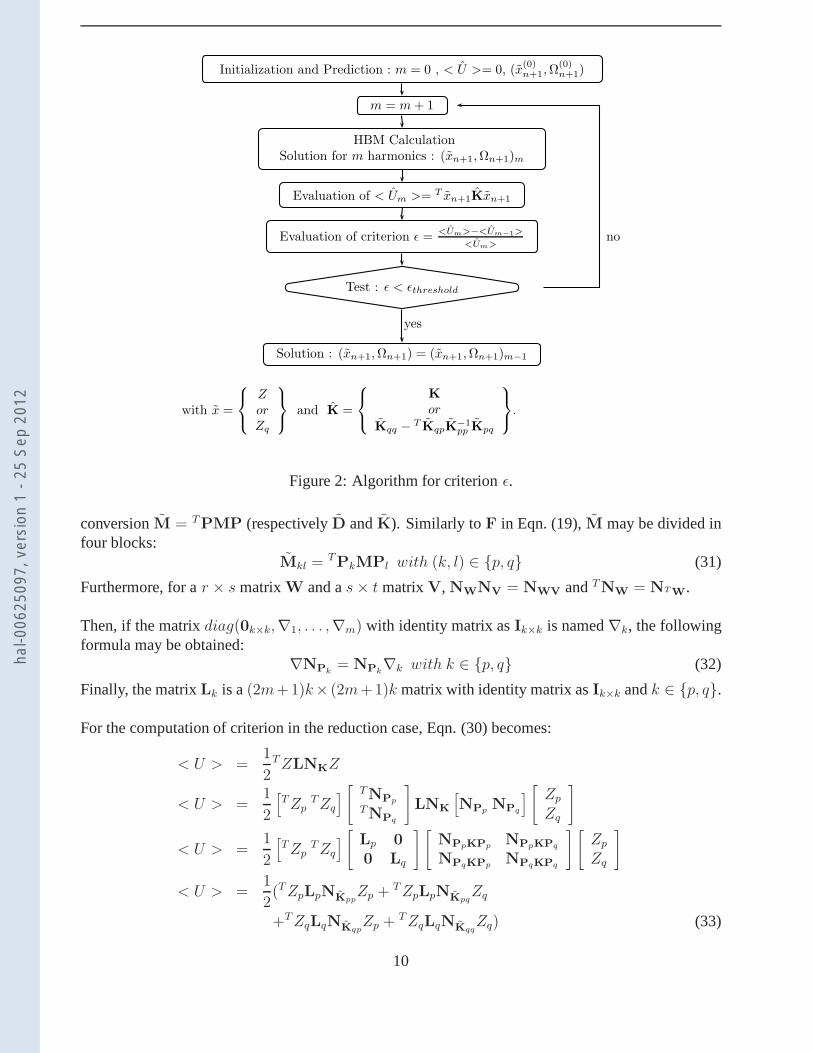
Criterion ǫ - The criterionǫ developed in this section is computed for a given frequency and thefirst resolution is performed for one harmonic. Then the relative difference between two consecutivevalues of strain energy is evaluated. The first value is obtained form harmonics and the second form + 1 harmonics. The increase is stopped whenǫ becomes less than a threshold chosen by user.Algorithm is detailed in Fig. 2.As matricesL andLq are diagonal constant block matrices and as algorithm starts for one harmonic,studying strain energy saturation is equivalent to studying saturation of an approximate quantity:

< U > = TZNKZ without condensation

< U > = TZqNKqq−T KqpK

−1pp Kpq

Zq with condensation (39)

Finally, when the convergence rate of the strain energy turns out to be non smooth, the method maystop before saturation. For example, for dry friction systems, only odd harmonics appear. However, asshown later, this drawback may be avoided removing all even harmonics in the calculation. For othercases, for example when the1st and5th harmonics responds, this drawback constitutes a limitation ofthe method.

11

hal-0

0625

097,

ver

sion

1 -

25 S

ep 2

012

3 Application Case

3.1 Two Beam System and Joint Model

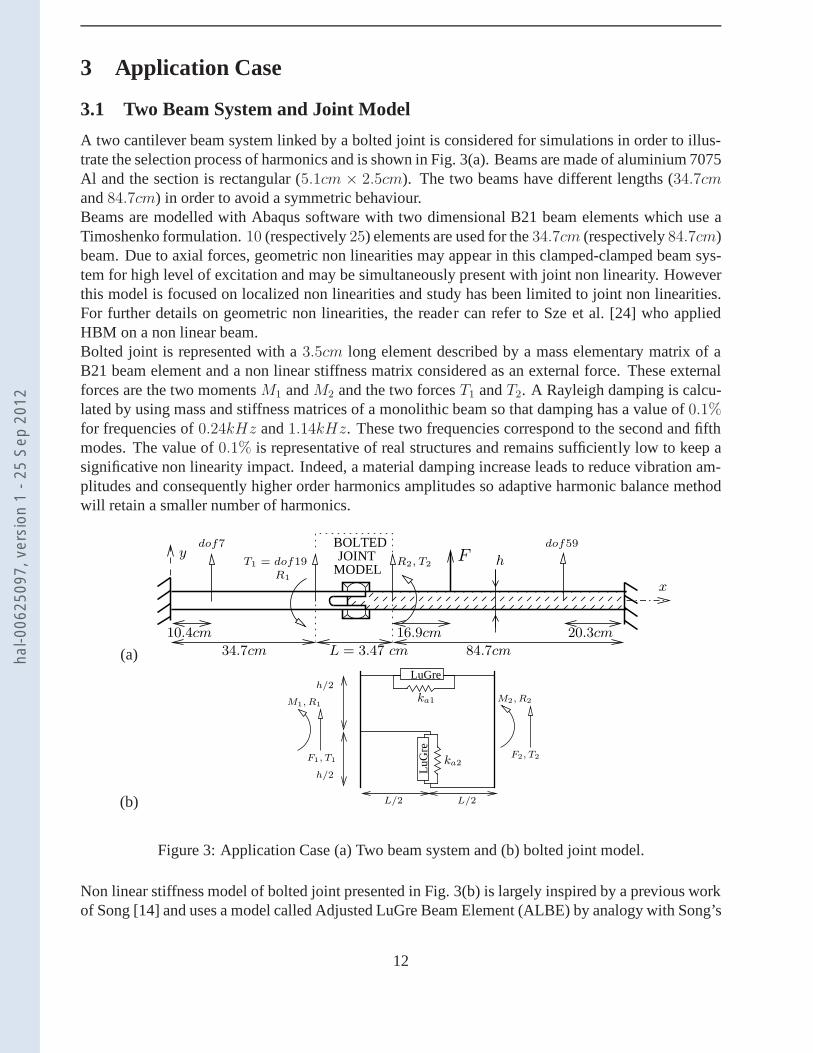
A two cantilever beam system linked by a bolted joint is considered for simulations in order to illus-trate the selection process of harmonics and is shown in Fig.3(a). Beams are made of aluminium 7075Al and the section is rectangular (5.1cm × 2.5cm). The two beams have different lengths (34.7cmand84.7cm) in order to avoid a symmetric behaviour.Beams are modelled with Abaqus software with two dimensional B21 beam elements which use aTimoshenko formulation.10 (respectively25) elements are used for the34.7cm (respectively84.7cm)beam. Due to axial forces, geometric non linearities may appear in this clamped-clamped beam sys-tem for high level of excitation and may be simultaneously present with joint non linearity. Howeverthis model is focused on localized non linearities and studyhas been limited to joint non linearities.For further details on geometric non linearities, the reader can refer to Sze et al. [24] who appliedHBM on a non linear beam.Bolted joint is represented with a3.5cm long element described by a mass elementary matrix of aB21 beam element and a non linear stiffness matrix considered as an external force. These externalforces are the two momentsM1 andM2 and the two forcesT1 andT2. A Rayleigh damping is calcu-lated by using mass and stiffness matrices of a monolithic beam so that damping has a value of0.1%for frequencies of0.24kHz and1.14kHz. These two frequencies correspond to the second and fifthmodes. The value of0.1% is representative of real structures and remains sufficiently low to keep asignificative non linearity impact. Indeed, a material damping increase leads to reduce vibration am-plitudes and consequently higher order harmonics amplitudes so adaptive harmonic balance methodwill retain a smaller number of harmonics.

(a)

MODEL

BOLTEDJOINT R2, T2

L = 3.47 cm 84.7cm34.7cm

y

x

F h

dof7 dof59

T1 = dof19R1

16.9cm10.4cm 20.3cm

(b)

LuGre

LuG

re

F2, T2

M2, R2ka1

ka2F1, T1

M1, R1

L/2 L/2

h/2

h/2

Figure 3: Application Case (a) Two beam system and (b) boltedjoint model.

Non linear stiffness model of bolted joint presented in Fig.3(b) is largely inspired by a previous workof Song [14] and uses a model called Adjusted LuGre Beam Element (ALBE) by analogy with Song’s

12

hal-0

0625

097,

ver

sion

1 -

25 S

ep 2

012

work. Frictional slip and slapping constitutes the two mainnon linear phenomena involved in the jointinterface [10]. However, for the sake of simplicity, slapping which can lead to higher order harmonicshas not been considered in this study. Frictional slip is here considered with a non linear modelintegrating a LuGre model leading to odd harmonics.As discussed in section 2.4, even harmonicshave to be removed in the HBM calculation so that smooth convergence rate of strain energy isobserved on only odd harmonics.The basic idea is to replace stiffnesses of a linear beam elementby a parallel combination of a LuGre model and a residual stiffnesska,i , i ∈ 1, 2 characteristic of abolted joint [11]. The element has two rotational dofsR1 andR2 and two translational dofsT1 andT2. h andL are respectively section height and element length.Spring elongations∆1 and∆2 have to be considered to express relation between non linearforceFNL,ALBE and element dofs:

∆1 =L

2(R1 +R2) + (T1 + T2) and ∆2 =

h

2(R1 − R2) (40)

Consequently each LuGre forcefLuGre,i , i ∈ 1, 2 depends on∆i elongation but also on internalvariable valueζi and its derivativeζi. It may be written as:

fLuGre,i(∆i, ∆i, ζi, ζi) = σ0i∆i + σ1iζi + α2i∆i (41)

ζi = ∆i −σ0i

α0i + α1ie−

(∆iv0i

)2

∣∣∣∆i

∣∣∣ ζi (42)

The combination of one LuGre model and one spring provides a force which takes the followingform:

fi(∆i, ∆i, ζi, ζi) = fLuGre,i(∆i, ∆i, ζi, ζi) + ka,i∆i (43)

Stiffness decrease during microslip regimes may be represented by using a coefficientγi ∈ [0; 1]which links the residual stiffnesska,i, the LuGre model stiffness parameterσ0i and the equivalentlinear element stiffnesski. The relative equations areσ0i = (1− γi)ki etka,i = γiki.ForcesF1, F2 and resulting momentsM1,M2 may be expressed as:

F1M1F2M2

=

f1(∆1, ∆1, ζ1, ζ1)L2f1(∆1, ∆1, ζ1, ζ1) +

h2f2(∆2, ∆2, ζ2, ζ2)

−f1(∆1, ∆1, ζ1, ζ1)L2f1(∆1, ∆1, ζ1, ζ1)−

h2f2(∆2, ∆2, ζ2, ζ2)

(44)

Thus from Eqn. (40) forcesFNL,ALBE may be written as a function of ALBE dofs:

FNL,ALBE(

T1

R1

T2

R2

,

˙

T1

R1

T2

R2

,

[

ζ1ζ2

]

,˙[

ζ1ζ2

]

) =

F1M1F2M2

(45)

The two equivalent linear element stiffnesseski are obtained by the following relations:

k1 = 12EI

L3= 1, 43.106N/mm et k2 = 4

EI

Lh2= 8, 92.105N/mm (46)

13

hal-0

0625

097,

ver

sion

1 -

25 S

ep 2

012

Other parameters are deduced by analogy with Shiryayev’s work [25], namelyγ1 = γ2 = 0.1078,α01 =α02 = 81.9N , σ11 = σ12 = α11 = α12 = α21 = α22 = 0. Finally σ01 = 1, 27.106N/mm, σ02 =7, 96.105N/mm, ka,1 = 1, 55.105N/mm, ka,2 = 9.62.104N/mm.

Then the system is excited with a harmonic excitationFL of 42N with a pulsationΩ. Load is appliedon the longest beam on translational dof31. By using formulation introduced in Eqn. (1), one maywrite the governing equation of motion to which two equations have to be added. These additionalequations describe LuGre model internal variablesζ1, ζ2 evolution:

MX +DX +KX = FL(Ω, t)− FNL,ALBE(

[

X

X

]

,

[

ζ1ζ2

]

,

[

ζ1ζ2

]

,Ω, t) (47)

ζi = ∆i −σ0i

α0i + α1ie−

(∆iv0i

)2

∣∣∣∆i

∣∣∣ ζi for i ∈ 1, 2 (48)

3.2 Adaptation of HBM Formulation to LuGre Model

In the studied case, two equations are added to the equation of motion and integrate non linear terms.Thus an adaptation of HBM formulation becomes necessary. Todo so, the two internal variablesζ1andζ2 are developed as a Fourier series in the same way asX. By inserting the truncatureζi(t) =T(t)Zζi into Eqn. (48), the same Galerkin method is applied on the resulting equation and one obtains:

0 = ζi −

∆i −

σ0i

α0i + α1ie−

(∆iv0i

)2

∣∣∣∆i

∣∣∣ ζi

0 = T(t)∇Zζi −T(t)bζi(Z,Zζi,Ω)

0 = NI1×1∇Zζi − bζi(Z,Zζi,Ω) with i ∈ 1, 2 (49)

wherebζi(Z,Zζi,Ω) are Fourier coefficients of the non linear term.

Consequently the problem is equivalent to finding zeros of a functionHH(Z,Zζ) depending onFourier coefficients ofX and ζ = [ζ1 ζ2]. These coefficients are namedZ andZζ = [Zζ1 Zζ2].HH is a function fromIR(2m+1)×(nddl+2) to IR(2∗m+1)×(nddl+2).

HH(Z,Zζ) =

H(Z,Zζ) = A(Ω)Z − b(Z,Zζ,Ω)C(Z,Zζ) = NI2×2

∇Zζ − bζ(Z,Zζ,Ω)

(50)

In case of condensation, we may define similarly a functionHHq(Zq, Zζ) from IR(2m+1)×(q+2) toIR(2∗m+1)×(q+2):

HHq(Zq, Zζ) =

Hq(Zq, Zζ) = Aq(Ω)Zq − bq(Zq, Zζ,Ω)C(Zq, Zζ) = NI2×2

∇Zζ − bq,ζ(Zq, Zζ,Ω)

(51)

Finally, calculation of approximate strain energy< U > stay the same as Eqn.(33) and Eqn. (38)because only Fourier coefficients of physical dofs are used to quantify strain energy.

14

hal-0

0625

097,

ver

sion

1 -

25 S

ep 2

012

3.3 Results

In the following, shown results have been calculated on the frequency band[0− 2.3] kHz with acurvilinear abscissa and an adaptive step to better describe resonance peaks. The Moore-Penrosemethod is used for correction at each iteration and prediction is made with Lagrange polynomials ofdegree2.

3.3.1 Non linear effects on dynamic responses

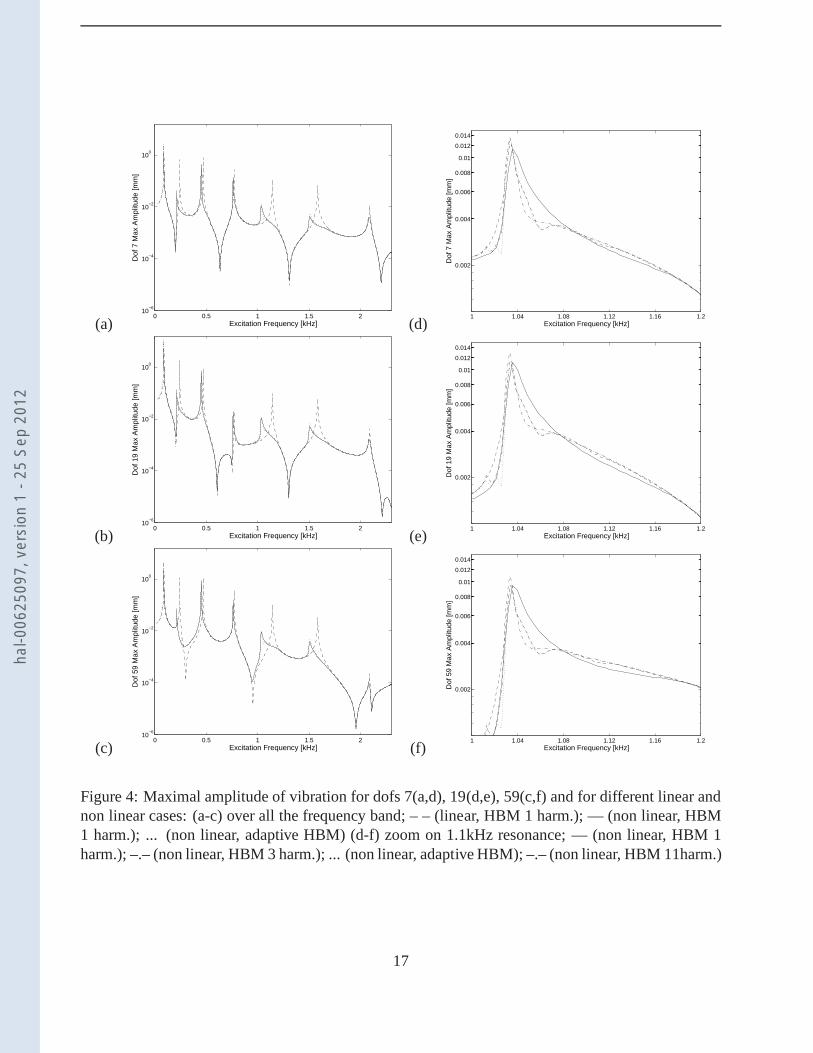
The maximal amplitude of vibration obtained for the linear case and for the two different non linearcases (1 harmonic case and adaptive case) are presented in Fig. 4(a,b,c) for the three dofs of the sys-tem. The1 harmonic case refers here to the classical HBM with one harmonic and does not refer toan adaptive algorithm. The first dof7 is located on the left beam, the second is a translational dof19corresponding to theR1 dof of the ALBE model, and the third one is the dof59 on the right beam.Figure. 3(a) details the dof position on the system. The threshold value for the relative variation ofthe approximate strain energy has been fixed to3% and excitation force has an amplitude of42N .The linear case shows seven modes on the studied frequency band. First non linearity effects aresignificant on the one harmonic response and result in two phenomena: a reduction of resonance peakamplitudes which reflects the damping from the joint and a modal softening which reflects the jointstiffness decrease. Thus some modes have important frequency shifts and even significant distortions,notably the second, fifth and sixth modes. Frequency shifts and vibration amplitude reductions havethe same order of magnitude for all the considered dofs. Differences are observed between the1harmonic curve and the adaptive algorithm near resonances especially near the fifth and sixth modeswhere the shape of peaks differs. Far from resonance peaks, adaptive algorithm give the same resultsas the1 harmonic calculation.

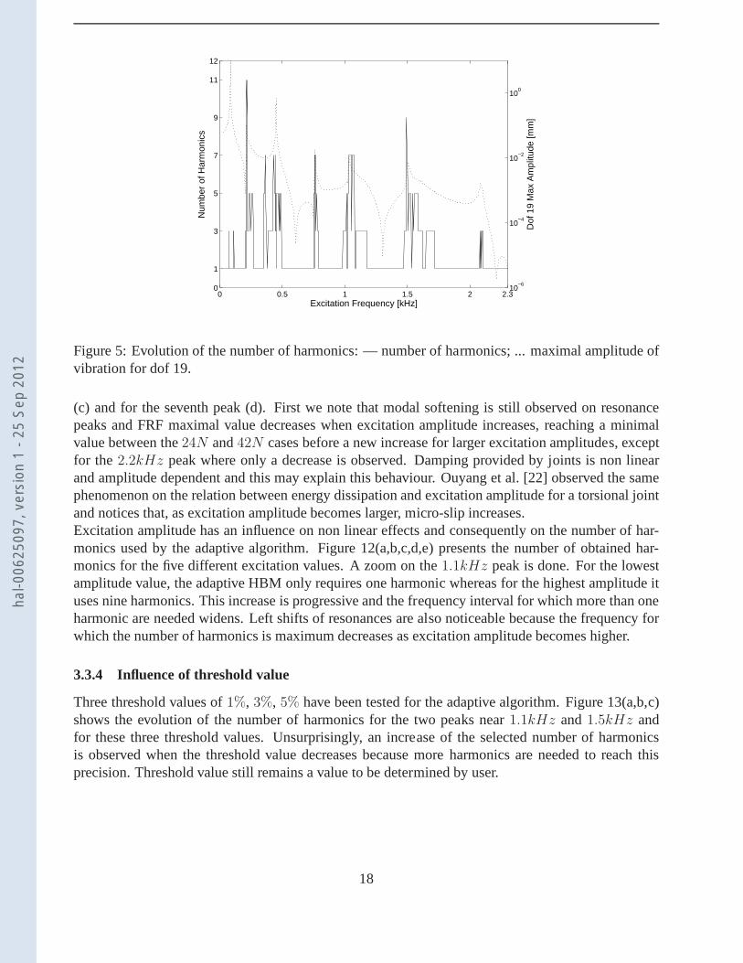
Figures 4(d,e,f) present a zoom on the1.1kHz resonance peak. Three non linear cases correspond-ing to a calculation with1, 3 and11 harmonics are compared with the adaptive HBM curve. Nearthe resonance, the adaptive HBM remains close to the response with 11 harmonics. However, Fig-ure 5, which plots the number of harmonics over the whole frequency band, shows that the numberof harmonics reaches only7 harmonics at most, revealing satisfying convergence of themethod. Thenumber of used harmonics may vary from1 to 11 for resonance peaks but only1 harmonic is nec-essary elsewhere. It shows that non linear phenomena are more pronounced on resonances. Themaximum number of harmonics has been fixed to 15 in this case.

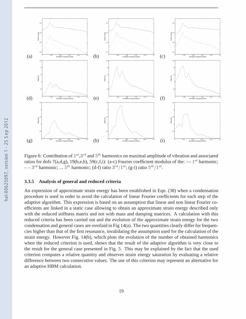
Contribution of each harmonic (1st,3rd and5th harmonic) is shown in Fig. 6(a,b,c) by plotting theFourier coefficient modulus of the1st,3rd and 5th harmonics of the vibration response (||Ak Bk||for harmonick and for one dof into Eqn. (2)) near the1.1kHz resonance peak. Analyses are stillperformed on the three dofs7, 19, and59. For the all three dofs, the1st harmonic contribution re-mains larger than the3rd and5th harmonic contributions. However, analysis of the ratios3rd/1st

(Fig 6(d,e,f)) and5th/1st (Fig 6(g,h,i)) shows that importance of third anf fifth harmonics increasesnear resonances and may represent up to10% for the third harmonic and up to2% for the fifth har-monic. This observation may be linked with the work of Ouyanget al. [22] who found emergenceof third and fifth superharmonics which represented about respectively2% and0.7% of the first har-monic. It may also be noted that third and fifth harmonics are less predominant for dof7 than for dofs

15

hal-0

0625

097,

ver

sion

1 -

25 S

ep 2

012

19 and59.A similar analysis on the approximate strain energy may be carried out by considering the contributionof the orderk as being the term1

2TZkKZk. Zk refers here to the contribution of the orderk to the

Fourier coefficient vectorZ of the vibration response. Results are plotted in Fig 7(a). Ratios3rd/1st

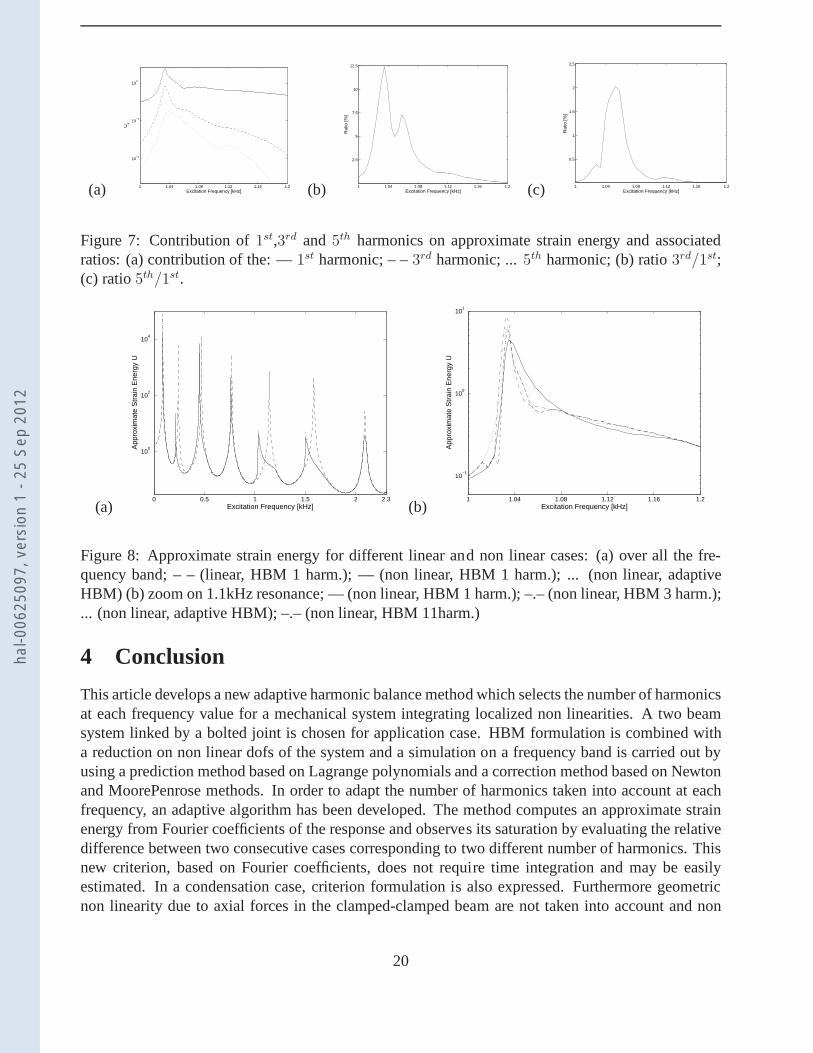
and5th/1st are shown in Fig 7(b,c). The same tendency that for maximal amplitude of vibration witha peak near resonance frequencies is observed. Moreover, ratios have the same order of magnitudewith a maximum value of12.5% for the third harmonic and of2% for the fifth harmonic, revealingthat approximate strain energy behaves like a global indicator of each dof behaviour.

3.3.2 Approximate Strain Energy Saturation

Approximate strain energy< U > is presented over all the frequency band for three cases on Fig. 8(a).The first case shows the shape of< U > for a linear case and a peak is observed for each resonancefrequency. The other two cases correspond to non linear calculations with one harmonic and withan adaptive number of harmonics. Non linear effects decrease vibration amplitude of the system sothat peaks on approximate strain energy are attenuated. As observed on the maximal amplitude ofvibration curves, peaks are shifted to the left. Moreover, differences between linear and non linearcases are predominant near resonance frequencies and adaptive algorithm curve differs from oneharmonic curve showing an increase in the required number ofharmonics. A zoom near the1.1kHzpeak is made on Fig. 8(b) in order to show convergence of the approximate strain energy quantity.Results are presented for1,3 and11 harmonics and for the adaptive case. Saturation is observedandadaptive case stays close to11 harmonic curve even if no more than9 harmonics are used.Finally, ithas to be noted that strain energy saturation is directly tested on odd harmonics due to the presence ofdry friction in the model and considered harmonics have a monotonous decrease of their amplitude. Itconstitutes a limitation of the method which cannot deal with non consecutive predominant harmonics(for example system with1, 3 and11 predominant harmonics).

3.3.3 Influence of force excitation

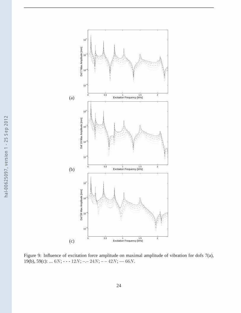
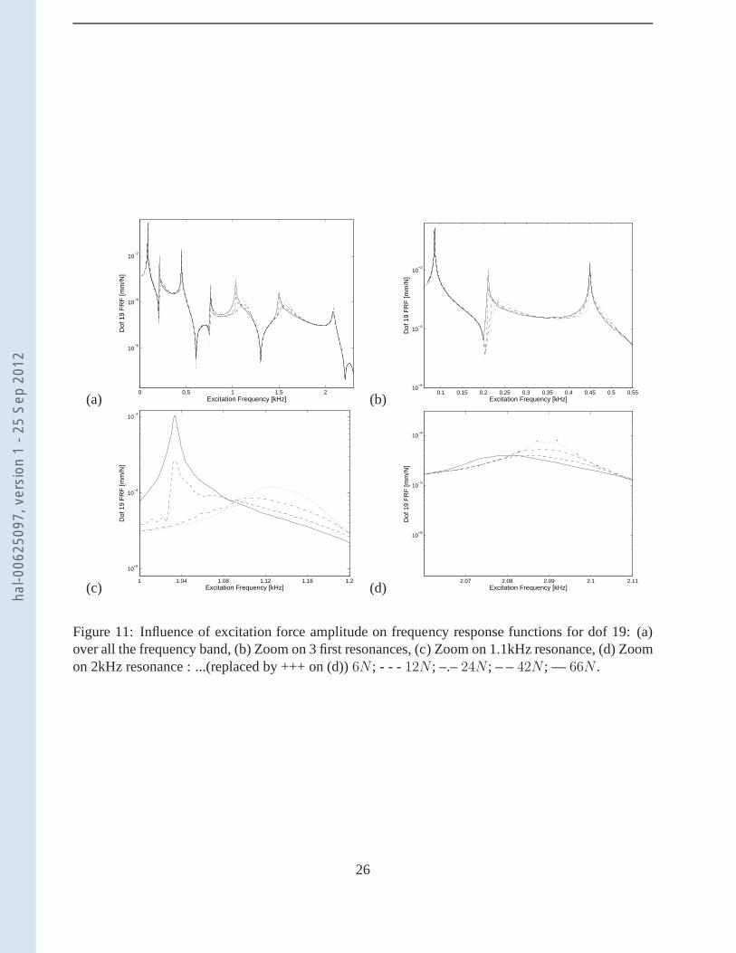
First simulations were carried out with an excitation amplitude of42N . Influence of excitation forceamplitude on non linear effects is now investigated by varying amplitude with the values6N , 12N ,24N , 42N , 66N . The maximal amplitude of vibration is presented for the three considered dofs inFig 9. Zooms for the dof19 are done for the first three peaks in Fig 9(a), for the fifth peakin Fig 9(b)and for the seventh peak in Fig 9(c). Responses are computed by using the adaptive algorithm. First,we note that an increase in excitation amplitude results in larger vibration amplitudes, and this forall the three dofs. Then, the main notable non linear effect is an increase in modal softening forlarger excitation amplitude, as shown by left shifts of resonance peaks. It clearly shows a relationshipbetween modal softening and vibration amplitudes and this dependence is non linear as previouslynoticed by Ungar [4]. For larger amplitudes, this modal softening becomes less remarkable revealingthe beginning of macro-slip and so the stabilization of the contact stiffness.In order to compare the five non linear cases, frequency response functions (FRFs) are computedby dividing the maximal amplitude of vibration by the excitation force amplitude for each frequencyvalue. Results, which are very similar for the three considered dofs, are presented in the particular caseof the dof19 in Fig 11 for all the frequency band (a), for the first three peaks (b), for the fifth peak

16

hal-0

0625

097,

ver

sion

1 -

25 S

ep 2

012

(a)0 0.5 1 1.5 2

10−6

10−4

10−2

100

Excitation Frequency [kHz]

Dof

7 M

ax A

mpl

itude

[mm

]

(d)1 1.04 1.08 1.12 1.16 1.2

0.002

0.004

0.006

0.008

0.01

0.012

0.014

Excitation Frequency [kHz]

Dof

7 M

ax A

mpl

itude

[mm

]

(b)0 0.5 1 1.5 2

10−6

10−4

10−2

100

Excitation Frequency [kHz]

Dof

19

Max

Am

plitu

de [m

m]

(e)1 1.04 1.08 1.12 1.16 1.2

0.002

0.004

0.006

0.008

0.01

0.012

0.014

Excitation Frequency [kHz]

Dof

19

Max

Am

plitu

de [m

m]

(c)0 0.5 1 1.5 2

10−6

10−4

10−2

100

Excitation Frequency [kHz]

Dof

59

Max

Am

plitu

de [m

m]

(f)1 1.04 1.08 1.12 1.16 1.2

0.002

0.004

0.006

0.008

0.01

0.012

0.014

Excitation Frequency [kHz]

Dof

59

Max

Am

plitu

de [m

m]

Figure 4: Maximal amplitude of vibration for dofs 7(a,d), 19(d,e), 59(c,f) and for different linear andnon linear cases: (a-c) over all the frequency band; – – (linear, HBM 1 harm.); — (non linear, HBM1 harm.); ... (non linear, adaptive HBM) (d-f) zoom on 1.1kHzresonance; — (non linear, HBM 1harm.); –.– (non linear, HBM 3 harm.); ... (non linear, adaptive HBM); –.– (non linear, HBM 11harm.)

17

hal-0

0625

097,

ver

sion

1 -

25 S

ep 2

012

0

1

3

5

7

9

11

12

Num

ber

of H

arm

onic

s

0 0.5 1 1.5 2 2.310

−6

10−4

10−2

100

Dof

19

Max

Am

plitu

de [m

m]

Excitation Frequency [kHz]

Figure 5: Evolution of the number of harmonics: — number of harmonics; ... maximal amplitude ofvibration for dof 19.

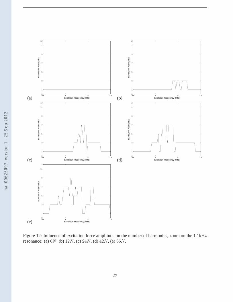
(c) and for the seventh peak (d). First we note that modal softening is still observed on resonancepeaks and FRF maximal value decreases when excitation amplitude increases, reaching a minimalvalue between the24N and42N cases before a new increase for larger excitation amplitudes, exceptfor the 2.2kHz peak where only a decrease is observed. Damping provided by joints is non linearand amplitude dependent and this may explain this behaviour. Ouyang et al. [22] observed the samephenomenon on the relation between energy dissipation and excitation amplitude for a torsional jointand notices that, as excitation amplitude becomes larger, micro-slip increases.Excitation amplitude has an influence on non linear effects and consequently on the number of har-monics used by the adaptive algorithm. Figure 12(a,b,c,d,e) presents the number of obtained har-monics for the five different excitation values. A zoom on the1.1kHz peak is done. For the lowestamplitude value, the adaptive HBM only requires one harmonic whereas for the highest amplitude ituses nine harmonics. This increase is progressive and the frequency interval for which more than oneharmonic are needed widens. Left shifts of resonances are also noticeable because the frequency forwhich the number of harmonics is maximum decreases as excitation amplitude becomes higher.

3.3.4 Influence of threshold value

Three threshold values of1%, 3%, 5% have been tested for the adaptive algorithm. Figure 13(a,b,c)shows the evolution of the number of harmonics for the two peaks near1.1kHz and1.5kHz andfor these three threshold values. Unsurprisingly, an increase of the selected number of harmonicsis observed when the threshold value decreases because moreharmonics are needed to reach thisprecision. Threshold value still remains a value to be determined by user.

18

hal-0

0625

097,

ver

sion

1 -

25 S

ep 2

012

(a) 1 1.04 1.08 1.12 1.16 1.2

10−5

10−4

10−3

10−2

Excitation Frequency [kHz]

Ord

er k

[mm

]

(b) 1 1.04 1.08 1.12 1.16 1.2

10−5

10−4

10−3

10−2

Excitation Frequency [kHz]

Ord

er k

[mm

]

(c) 1 1.04 1.08 1.12 1.16 1.2

10−5

10−4

10−3

10−2

Excitation Frequency [kHz]

Ord

er k

[mm

]

(d) 1 1.04 1.08 1.12 1.16 1.2

2.5

5

7.5

10

12.5

Excitation Frequency [kHz]

Rat

io [%

]

(e) 1 1.04 1.08 1.12 1.16 1.2

2.5

5

7.5

10

12.5

Excitation Frequency [kHz]

Rat

io [%

]

(f) 1 1.04 1.08 1.12 1.16 1.2

2.5

5

7.5

10

12.5

Excitation Frequency [kHz]

Rat

io [%

]

(g) 1 1.04 1.08 1.12 1.16 1.2

0.5

1

1.5

2

2.5

Excitation Frequency [kHz]

Rat

io [%

]

(h) 1 1.04 1.08 1.12 1.16 1.2

0.5

1

1.5

2

2.5

Excitation Frequency [kHz]

Rat

io [%

]

(i) 1 1.04 1.08 1.12 1.16 1.2

0.5

1

1.5

2

2.5

Excitation Frequency [kHz]

Rat

io [%

]

Figure 6: Contribution of1st,3rd and5th harmonics on maximal amplitude of vibration and associatedratios for dofs 7(a,d,g), 19(b,e,h), 59(c,f,i): (a-c) Fourier coefficient modulus of the: —1st harmonic;– –3rd harmonic; ...5th harmonic; (d-f) ratio3rd/1st; (g-i) ratio 5th/1st.

3.3.5 Analysis of general and reduced criteria

An expression of approximate strain energy has been established in Eqn. (38) when a condensationprocedure is used in order to avoid the calculation of linearFourier coefficients for each step of theadaptive algorithm. This expression is based on an assumption that linear and non linear Fourier co-efficients are linked in a static case allowing to obtain an approximate strain energy described onlywith the reduced stiffness matrix and not with mass and damping matrices. A calculation with thisreduced criteria has been carried out and the evolution of the approximate strain energy for the twocondensation and general cases are overlaid in Fig 14(a). The two quantities clearly differ for frequen-cies higher than that of the first resonance, invalidating the assumption used for the calculation of thestrain energy. However Fig. 14(b), which plots the evolution of the number of obtained harmonicswhen the reduced criterion is used, shows that the result of the adaptive algorithm is very close tothe result for the general case presented in Fig. 5. This may be explained by the fact that the usedcriterion computes a relative quantity and observes strainenergy saturation by evaluating a relativedifference between two consecutive values. The use of this criterion may represent an alternative foran adaptive HBM calculation.

19

hal-0

0625

097,

ver

sion

1 -

25 S

ep 2

012

(a) 1 1.04 1.08 1.12 1.16 1.2

10−4

10−2

100

Excitation Frequency [kHz]

Uk

(b) 1 1.04 1.08 1.12 1.16 1.2

2.5

5

7.5

10

12.5

Excitation Frequency [kHz]

Rat

io [%

]

(c) 1 1.04 1.08 1.12 1.16 1.2

0.5

1

1.5

2

2.5

Excitation Frequency [kHz]

Rat

io [%

]

Figure 7: Contribution of1st,3rd and 5th harmonics on approximate strain energy and associatedratios: (a) contribution of the: —1st harmonic; – –3rd harmonic; ...5th harmonic; (b) ratio3rd/1st;(c) ratio5th/1st.

(a)0 0.5 1 1.5 2 2.3

100

102

104

Excitation Frequency [kHz]

App

roxi

mat

e S

trai

n E

nerg

y U

(b)1 1.04 1.08 1.12 1.16 1.2

10−1

100

101

Excitation Frequency [kHz]

App

roxi

mat

e S

trai

n E

nerg

y U

Figure 8: Approximate strain energy for different linear and non linear cases: (a) over all the fre-quency band; – – (linear, HBM 1 harm.); — (non linear, HBM 1 harm.); ... (non linear, adaptiveHBM) (b) zoom on 1.1kHz resonance; — (non linear, HBM 1 harm.); –.– (non linear, HBM 3 harm.);... (non linear, adaptive HBM); –.– (non linear, HBM 11harm.)

4 Conclusion

This article develops a new adaptive harmonic balance method which selects the number of harmonicsat each frequency value for a mechanical system integratinglocalized non linearities. A two beamsystem linked by a bolted joint is chosen for application case. HBM formulation is combined witha reduction on non linear dofs of the system and a simulation on a frequency band is carried out byusing a prediction method based on Lagrange polynomials anda correction method based on Newtonand MoorePenrose methods. In order to adapt the number of harmonics taken into account at eachfrequency, an adaptive algorithm has been developed. The method computes an approximate strainenergy from Fourier coefficients of the response and observes its saturation by evaluating the relativedifference between two consecutive cases corresponding totwo different number of harmonics. Thisnew criterion, based on Fourier coefficients, does not require time integration and may be easilyestimated. In a condensation case, criterion formulation is also expressed. Furthermore geometricnon linearity due to axial forces in the clamped-clamped beam are not taken into account and non

20

hal-0

0625

097,

ver

sion

1 -

25 S

ep 2

012

linear effects in the joint consider only frictional slip. Slapping is not modelled in this study. Slip inthe bolted joint element is represented by a LuGre model which leads to adapt the HBM formulationin order to develop internal variables as Fourier series.Results show that one harmonic is sufficient to give a satisfactory approximation of the response awayfrom resonances and is necessary to highlight non linear effects such as damping of resonance peaksand modal softening. Indeed the dynamic behaviour is strongly modified compared with the linearcase. Moreover, adaptive HBM shows that, for a given threshold value of the criterion, the numberof harmonics may increase on resonances indicating that nonlinear effects are predominant. Theevolution of the approximate strain energy shows that a peakis observed near each resonance andsaturation of this quantity is noted when the number of harmonics increases.However, calculationis performed only on odd harmonics due to dry friction leading to a smooth convergence rate ofthe strain energy on tested harmonics. This condition constitutes a limitation of the method whichcannot deal with non consecutive predominant harmonics (for example system with predominantharmonics1, 3 and11). Analysis of each harmonic contribution notices the emergence of third andfifth harmonics both on the response and on approximate strain energy near resonances, showingthe global characteristic of the criterion based on approximate strain energy. In order to obtain awider range of harmonics and to model a more physical bolted system, slapping and geometric nonlinearities could be considered for further work. A coherent behaviour is noticed when thresholdvalue varies because more harmonics are needed to reach the given precision when threshold value ofthe adaptive algorithm is decreased.A parametric study is carried out by varying the excitation force amplitude. Vibration amplitudeincreases with higher force amplitude because non linear effects, notably micro slip in the joint,become more pronounced. Modal softening and damping depends on vibration amplitude and thisdependency is non linear. Maximum of frequency response functions for each resonance dependsnon linearly on excitation amplitude and may reach a minimumvalue for an intermediate excitationamplitude. The number of needed harmonics becomes larger for increasing amplitudes underliningthe predominance of non linear effects.

References

[1] D. J. Segalman. Modelling joint friction in structural dynamics.Journal of Sound and Vibration,13(1):430–453, 2005.

[2] L. Gaul and R. Nitsche. The role of friction in mechanicaljoints. Applied Mechanics Reviews,54(2):93–106, 2001.

[3] C. F. Beards. Damping in structural joints.The shock and vibration digest, 24(7):3–7, 1992.

[4] E. E. Ungar. Status of engineering knowledge concerningdamping of built-up structures.Jour-nal of Sound and Vibration, 26(1):141–154, 1973.

[5] R. A. Ibrahim and C. L. Pettit. Uncertainties and dynamicproblems of bolted joints and otherfasteners.Journal of Sound and Vibration,, 279(3-5):857–936, 2005.

21

hal-0

0625

097,

ver

sion

1 -

25 S

ep 2

012

[6] H. Ahmadian, J. E. Mottershead, S. James, M. I. Friswell,and C. A. Reece. Modelling andupdating of large surface-to-surface joints in the awe-mace structure.Mechanical Systems andSignal Processing, 20(4):868–880, 2006.

[7] A. D. Crocombe, R. Wang, G. Richardson, and C. I. Underwood. Estimating the energy dissi-pated in a bolted spacecraft at resonance.Computers & Structures, 84(5-6):340–350, 2006.

[8] R. Wang, A. D. Crocombe, G. Richardson, and C. I. Underwood. Energy dissipation in space-craft structures incorporating bolted joints operating inmacroslip.Journal of Aerospace Engi-neering, 21(1):19–26, 2008.

[9] A. Caignot, P. Ladeveze, D. Neron, V. Le Gallo, and L. Gonidou. Virtual testing for the pre-diction of damping in joints. ICED 2007 International Conference in Engineering Dynamics,2007.

[10] H. Ahmadian and H. Jalali. Generic element formulationfor modelling bolted lap joints.Me-chanical Systems and Signal Processing, 21(5):2318–2334, 2007.

[11] L. Gaul and J. Lenz. Nonlinear dynamics of structures assembled by bolted joints.Acta Me-chanica, 125(1-4):169–181, 1997.

[12] M. J. Oldfield, H. Ouyang, and J. E. Mottershead. Simplified models of bolted joints underharmonic loading.Computers & Structures,, 84(1-2):25–33, 12 2005.

[13] H. Ahmadian and H. Jalali. Identification of bolted lap joints parameters in assembled structures.Mechanical Systems and Signal Processing, 21(2):1041–1050, 2007.

[14] Y. Song, C. J. Hartwigsen, D. M. McFarland, A. F. Vakakis, and L. A. Bergman. Simulation ofdynamics of beam structures with bolted joints using adjusted iwan beam elements.Journal ofSound and Vibration, 273(1-2):249–276, 2004.

[15] J. D. Miller and D. D. Quinn. A two-sided interface modelfor dissipation in structural systemswith frictional joints. Journal of Sound and Vibration, 321(1-2):201–219, 2009.

[16] L. Heller, E. Foltete, and J. Piranda. Experimental identification of nonlinear dynamic propertiesof built-up structures.Journal of Sound and Vibration, 327(1-2):183–196, 2009.

[17] C. Pierre, A. A. Ferri, and E. H. Dowell. Multi-harmonicanalysis of dry friction damped systemsusing an incremental harmonic-balance method.Journal of Applied Mechanics-Transactions ofthe Asme, 52(4):958–964, 1985.

[18] A. A. Ferri and E. H. Dowell. Frequency-domain solutions to multi-degree-of-freedom, dryfriction damped systems.Journal of Sound and Vibration, 124(2):207–224, 1988.

[19] T. M. Cameron and J. H. Griffin. An alternating frequency/time domain method for calculat-ing the steady-state response of nonlinear dynamic systems. Journal of Applied Mechanics-Transactions of the Asme, 56(1):149–154, 1989.

22

hal-0

0625

097,

ver

sion

1 -

25 S

ep 2

012

[20] N. Coudeyras, J.-J. Sinou, and S. Nacivet. A new treatment for predicting the self-excitedvibrations of nonlinear systems with frictional interfaces: The constrained harmonic balancemethod, with application to disc brake squeal.Journal of Sound and Vibration, 319(3-5):1175–1199, 2009.

[21] Y. Ren, T. M. Lim, and M. K. Lim. Identification of properties of nonlinear joints using dynamictest data.Journal of Vibration and Acoustics-Transactions of the Asme, 120(2):324–330, 1998.

[22] H. Ouyang, M. J. Oldfield, and J. E. Mottershead. Experimental and theoretical studies of abolted joint excited by a torsional dynamic load.International Journal of Mechanical Sciences,48(12):1447–1455, 2006.

[23] D. Laxalde.Etude d’amortisseurs non-lineaires appliques aux roues aubagees et aux systemesmulti-etages. PhD thesis, Ecole Centrale de Lyon, 2007.

[24] K.Y. Sze, S.H. Chen, and J.L. Huang. The incremental harmonic balance method for non linearvibration of axially moving beams.Journal of Sound and Vibration, 281:611–626, 2005.

[25] O. V. Shiryayev, S. M. Page, C. L. Pettit, and J. C. Slater. Parameter estimation and investigationof a bolted joint model.Journal of Sound and Vibration, 307(3-5):680–697, 2007.

23

hal-0

0625

097,

ver

sion

1 -

25 S

ep 2

012

(a)0 0.5 1 1.5 2

10−6

10−4

10−2

100

Excitation Frequency [kHz]

Dof

7 M

ax A

mpl

itude

[mm

]

(b)0 0.5 1 1.5 2

10−6

10−4

10−2

100

Excitation Frequency [kHz]

Dof

19

Max

Am

plitu

de [m

m]

(c)0 0.5 1 1.5 2

10−6

10−4

10−2

100

Excitation Frequency [kHz]

Dof

59

Max

Am

plitu

de [m

m]

Figure 9: Influence of excitation force amplitude on maximalamplitude of vibration for dofs 7(a),19(b), 59(c): ...6N ; - - - 12N ; –.–24N ; – –42N ; — 66N .

24

hal-0

0625

097,

ver

sion

1 -

25 S

ep 2

012

(a)0.1 0.15 0.2 0.25 0.3 0.35 0.4 0.45 0.5 0.55 0.6

10−4

10−2

100

Excitation Frequency [kHz]

Dof

19

Max

Am

plitu

de [m

m]

(b)1 1.04 1.08 1.12 1.16 1.2

10−4

10−3

10−2

Excitation Frequency [kHz]

Dof

19

Max

Am

plitu

de [m

m]

(c)2.04 2.06 2.08 2.1 2.12 2.14

10−6

10−5

10−4

10−3

Excitation Frequency [kHz]

Dof

19

Max

Am

plitu

de [m

m]

Figure 10: Influence of excitation force amplitude on maximal amplitude of vibration for dof 19:(a) Zoom on 3 first resonances, (b) Zoom on 1.1kHz resonance, (c) Zoom on 2kHz resonance: ...(replaced by +++ on (c))6N ; - - - 12N ; –.–24N ; – –42N ; — 66N .

25

hal-0

0625

097,

ver

sion

1 -

25 S

ep 2

012

(a)0 0.5 1 1.5 2

10−6

10−4

10−2

Excitation Frequency [kHz]

Dof

19

FR

F [m

m/N

]

(b)0.1 0.15 0.2 0.25 0.3 0.35 0.4 0.45 0.5 0.55

10−6

10−4

10−2

Excitation Frequency [kHz]D

of 1

9 F

RF

[mm

/N]

(c)1 1.04 1.08 1.12 1.16 1.2

10−5

10−4

10−3

Excitation Frequency [kHz]

Dof

19

FR

F [m

m/N

]

(d)2.07 2.08 2.09 2.1 2.11

10−6

10−5

10−4

Excitation Frequency [kHz]

Dof

19

FR

F [m

m/N

]

Figure 11: Influence of excitation force amplitude on frequency response functions for dof 19: (a)over all the frequency band, (b) Zoom on 3 first resonances, (c) Zoom on 1.1kHz resonance, (d) Zoomon 2kHz resonance : ...(replaced by +++ on (d))6N ; - - - 12N ; –.–24N ; – –42N ; — 66N .

26

hal-0

0625

097,

ver

sion

1 -

25 S

ep 2

012

(a)0.9 1 1.1 1.20

1

3

5

7

9

11

12

Excitation Frequency [kHz]

Num

ber

of H

arm

onic

s

(b)0.9 1 1.1 1.20

1

3

5

7

9

11

12

Excitation Frequency [kHz]

Num

ber

of H

arm

onic

s

(c)0.9 1 1.1 1.20

1

3

5

7

9

11

12

Excitation Frequency [kHz]

Num

ber

of H

arm

onic

s

(d)0.9 1 1.1 1.20

1

3

5

7

9

11

12

Excitation Frequency [kHz]

Num

ber

of H

arm

onic

s

(e)0.9 1 1.1 1.20

1

3

5

7

9

11

12

Excitation Frequency [kHz]

Num

ber

of H

arm

onic

s

Figure 12: Influence of excitation force amplitude on the number of harmonics, zoom on the 1.1kHzresonance: (a)6N , (b) 12N , (c) 24N , (d) 42N , (e)66N .

27

hal-0

0625

097,

ver

sion

1 -

25 S

ep 2

012

(a) 0.9 1 1.2 1.4 1.6 1.8 1.90

1

3

5

7

9

11

12

Excitation Frequency [kHz]

Num

ber

of H

arm

onic

s

(b) 0.9 1 1.2 1.4 1.6 1.8 1.90

1

3

5

7

9

11

12

Excitation Frequency [kHz]

Num

ber

of H

arm

onic

s

(c) 0.9 1 1.2 1.4 1.6 1.8 1.90

1

3

5

7

9

11

12

Excitation Frequency [kHz]

Num

ber

of H

arm

onic

s

Figure 13: Influence of threshold value on the number of harmonics, zoom on the 1.1kHz and the1.5kHz resonances: (a)5%, (b) 3%, (c) 1%.

(a)0 0.5 1 1.5 2 2.3

10−4

10−2

100

102

104

Excitation Frequency [kHz]

App

roxi

mat

e S

trai

n E

nerg

y

(b)0 0.5 1 1.5 2 2.3

0

1

3

5

7

9

11

12

Excitation Frequency [kHz]

Num

ber

of H

arm

onic

s

Figure 14: (a) Approximate strain energy: — general expression; – – condensation case expression(b)Number of harmonics obtained with the condensation caseexpression.

28

hal-0

0625

097,

ver

sion

1 -

25 S

ep 2

012