AN ABSTRACT OF THE THESIS OF of Thiophene and ...

AN ABSTRACT OF THE THESIS OF

All H. Al-Raie for the degree of Master of Science in Chemical Engineering

presented on March 10, 2005.

Title: Desulfurization of Thiophene and Dibenzothiophene with Hydrogen

Peroxide in a Photochemical Microreactor.

Abstract approved:

Dr. Gbân N. Jovanovic

Sulfur content of fuels and desulfurization of fuels is becoming an

important environmental restriction and regulatory issue. In this study new

technology for the desulfurization of fuels is considered. Micro scale reactors are

introduced for desulfurization of thiophene and dibenzothiophene.

Thiophene and dibenzothiophene are mixed with hexane at concentration,

C0 of 300 ppm. The mixture is introduced into the microreactor concurrently with

hydrogen peroxide in equal volumetric flow rates. The two reactant steams form

two thin layers inside the microreactor. The microreactor is 2.2 cm long, and 1.05

cm wide. Thin spacers, 100 pm and 50 pm, are used to establish the thickness of

the microchannels. The microreactor is housed between stainless steel plates

which have rectangular windows to facilitate UV irradiation of the reaction

Redacted for Privacy

mixture. UV light helps the desulfurization reaction to proceed. The overall

desulfurization process for both thiophene and dibenzothiophene is a pseudo

first-order reaction. The thiophene and dobenzothiophene reacted with hydroxyl

radicals to form their respective sulfoxides and sulfones.

The experiments are conducted at room temperature, and at steady state

conditions. The ranges of the operating conditions are: the residence time, 0.15

to 9.59 (mm.), the spacer thickness (half-thickness of the reactor), 50 and 100

(tm), and the distance between the microreactor and the UV light source, 1.5 to

6.0 (cm). The thiophenes desulfurization study includes, comparison between

model and experimental results, comparison between thiophene and

dibenzothiophene reactivity, the effect of the spacer thickness, the effect of the

UV light source distance, and comparison between results obtained by

introducing the microreactor and to those obtained from batch process done by

other researchers.

A mathematical model reflecting geometry and flow conditions inside the

microreactor is developed to predict the conversion of thiophene and

dibezothiophene. The model includes axial convection and diffusion, lateral

diffusion, and pseudo first order reaction kinetics at the interface between the two

reactant streams. The model is solved numerically using FEMLAB (Finite

Element Method Laboratory) software package. The experimental data are fitted

to the model equations and the pseudo first order reaction rate constant (k) is

evaluated. It is found that the reaction rate constant for thiophene is 1.31*107

[mis] for spacer thickness of 100 jim, and I .33*107 rn/s for spacer thickness of

50 jim. The reaction rate for the desulfurization of dibenzothiophene is 1.47*107

(m/s). It is found that the mathematical model explained the experimental data

very well. Therefore, the model developed in this study may be used to design

desulfurization processes and to predict the concentration profile in the

micro reactor.

In general, the microreactor was much more efficient in desulfurization of

thiophene and dibenzothiophene when compared to other batch processes. The

microreactor was capable of achieving 98.20% conversion at 8.11 minutes mean

residence time for thiophene desulfurizationthus, thus reducing the thiophene

concentration from 300 ppm to less than 6 ppm.

©Copyright by Au H. Al-Raie

March 10, 2005

All Rights Reserved

Desulfurization of Thiophene and Dibenzothiophene withHydrogen Peroxide in a Photochemical Microreactor

by

All H. Al-Raie

A THESIS

submitted to

Oregon State University

in partial fulfillment of

the requirements for the

degree of

Master of Science

Presented March 10, 2005

Commencement June 2005

Master of Science thesis of Au H. Al-Raie presented on March 10, 2005.

APPROVED:

Major Professcfr'fep Chemical Engineering

Head of the Department of Chemical Engineering

Dean of the Grad

I understand that my thesis will become part of the permanent collection of

Oregon State University libraries. My signature below authorizes release of my

thesis to any reader upon request.

Ali H. Al-Faie, Author





ACKNOWLEDGEMENTS

My special thanks go to my parents, wife, and brothers for the support I

had during this challenging time.

I wish to express my sincere appreciation to my major professor, Dr.

Goran Jovanovic, to whom I owe very much in many respects. His excellent

instruction during my graduate studies and professional guidance has helped me

to accomplish this degree.

I must also thank Dr. Eric Henry for his great support during setting up the

experimental apparatus, and for his helpful information and recommendations.

I would also like to thank Khalid Alkhaldi, Carlos Cruz-Fierro, Brian Reed,

and Ahmed Aldhubabian for their great support in computer modeling, setting up

the microreactor, and HPLC analysis which were crucial for the completion of my

thesis.

Also, I would like to thank Saudi Aramco Company for the financial

support during my study at Oregon State University.

TABLE OF CONTENTS

PageI INTRODUCTION. I

1.1 Fuels Sulfur Content Regulations ......................................... 4

1.1.1 Sulfur Content and Particulate Emission ........................ 41.1.2 Diesel Sulfur Standards in the USA .............................. 51.1.3 Diesel Sulfur Standards in Canada ............................... 61.1.4 Diesel Sulfur Standards in the European Union ............... 71.1.5 Diesel Sulfur Standards in the Asia-Pacific Region ........... 81.1.6 Diesel Sulfur Standards in Central and South America 81.1.7 The World-Wide Fuel Charter...................................... 9

1.2 State of The Art of Microreaction Technology.......................... 10

1.2.1 Definition ................................................................. 111.2.2 Fundamental Advantages of Microreactors..................... 121.2.3 Functional Classification of Microreactors ...................... 151.2.4 Analysis vs. Production Microstructured Sysytems ........... 161.2.5 Potential Benefits of Microstructured Systems................. 17

1.3 Goal and Objectives .......................................................... 20

2 REACTION MECHANISM OF THIOPHENES OXIDATION .............. 21

2.1 Desulfurization of Thiophene Derivatives ............................... 21

2.2 Reaction Kinetics .............................................................. 24

3 THEORETICAL ELEMENTS ...................................................... 28

3.1 Velocity Profile.................................................................. 28

3.1.1 Assumptions............................................................ 293.1.2 Continuity Equation ................................................... 293.1.3 Equations of Motion ................................................... 303.1.4 Determination of The Ratio of Layers Thicknesses ........... 333.1.5 Determination of the Pressure Drop .............................. 36

TABLE OF CONTENTS (Continued)

Page

3.2 Mathematical Modeling ...................................................... 38

3.2.1 Assumptions ............................................................ 403.2.2 Mathematical Model .................................................. 413.2.3 Model Dimensionless Format...................................... 43

4 EXPERIMENTAL APPARATUS AND PROCEDURE ....................... 45

4.1 Materials ......................................................................... 45

4.2 Equipments..................................................................... 46

4.3 Method ........................................................................... 51

4.3.1 Desulfurization of Thiophene and dibenzothiophene ......... 514.3.2 Determination of Thiophene and Dibenzothiophene

Concentration ........................................................... 55

5 EXPERIMENTAL MEASUREMENTS .......................................... 58

5.1 Desulfurization without UV Light............................................ 58

5.2 Desulphurization of Thiophene under UV Light........................ 60

5.3 Desulphurization of Dibenzothiophene under UV Light.............. 65

6 RESULTS AND DISCUSSION ................................................... 68

6.1 Experimental Results and Models ......................................... 69

6.1.1 Desulphurization of Thiophene .................................... 696.1.2 Desulphurization of Dibenzothiophene .......................... 85

6.2 Comparison between Thiophene and Dibenzothiophene ........... 93

6.3 Effect of Spacer Thickness .................................................. 94

6.4 Effect of UV source Distance ............................................... 95

6.5 Comparison with Other Researchers' Work............................. 96

TABLE OF CONTENTS (Continued)

Page

7 CONCLUSION AND RECOMMENDATIONS ................................. 99

7.1 Conclusion ...................................................................... 99

7.2 Recommendations ............................................................ 105

BIBLIOGRAPHY ......................................................................... 108

APPENDICES ............................................................................ 112

LIST OF FIGURES

Figure Page

1.1 Hydrodesulfurization process ................................................ 3

1.2 Microchannels reactor ......................................................... 11

3.1 Schematic of the velocity profile inside the microrector ............... 28

3.2 Actual velocity profile inside the microrector. Ba91.304 pm,Bb=108.696 tm, MRT=5.02 mm., AP= 0.11 Pa, J.ta=3.3*1 0 Pa.s,}1b9.OlO .......................................................................... 37

3.3 Schematic of the microrector channels .................................... 39

3.4 Control element inside the microrector .................................... 39

4.1 Syringe pump .................................................................... 46

4.2 Exploded sketch of the microreactor parts ............................... 48

4.3 Exploded view of the microreactor parts .................................. 49

4.4 Front view of the microreactor............................................... 49

4.5 Side view of the microreactor ................................................ 50

4.6 HPLC system ..................................................................... 51

4.7 Experimental setup............................................................. 53

4.8 Formation of layers inside the microreactor .............................. 54

4.9 Chromatograph of thiophene ................................................ 56

4.10 Chromatograph of dibenzothiophene ...................................... 56

5.1 Concentration profile of thiophene vs. time for the sample mixedwith 30% hydrogen peroxide in a vial contained in a cold box. C0

= 300 ppm thiophene in hexane ............................................. 59

5.2 Concentration profile of dibenzothiophene vs. time for the samplemixed with 30% hydrogen peroxide in a vial contained in a coldbox. C0 = 300 ppm dibenzothiophene in hexane ............................ 59

LIST OF FIGURES (Continued)

Figure Page

5.3 Cromtograph of thiophene sample. C0=300 ppm, L=2.20*102 m,w=1.05*102 m, spacer thickness is 50 jtm, £=5.0*103 m,MRT=0.15 mm., T=25 °C..................................................... 62

5.4 Concentration profile of thiophene vs. mean residence time.C0=300 ppm, L=2.20*102 m, w=1.05*1O2 m, spacer thickness is100 jim, £=1.5*102m, T=25 °C .............................................. 62

5.5 Concentration profile of thiophene vs. mean residence time.C0=300 ppm, L=2.20*102 m, w=1.05*102 m, spacer thickness is5Ojim, £=1.5*102m,T=250C 63

5.6 Profile of thiophene conversion vs. Distance of UV light source.C0=300 ppm, L=2.20*102 m, w=l.05*102 m, spacer thickness is100 jim, MRT=6.59 mm., T=25 °C .......................................... 64

5.7 Cromtograph of dibenzothiophene sample. C0300 ppm,L=2.20*102 m, w=1.05*102 m, spacer thickness is 100 jim,£=1.5*102m, MRT=3.40 mm., T=25 °C ................................... 66

5.8 Concentration profile of dibenzothiophene vs. mean residencetime. C0=300 ppm, L=2.20*102 m, w=1.05*102 m, spacerthickness is 100 Jim, £=1.5*102m, T=25 °C ............................. 66

6.1 Concentration profile of thiophene vs. mean residence time formodel and experiments. C0=300 ppm, L=2.20*102 m, w=1.05*102 m, spacer thickness is 100 jim, £=1.5*102m, T=25 °C .............. 71

6.2 Concentration profile of thiophene vs. mean residence time formodel and experiments. C0=300 ppm, L=2.20*102 m, w1 .05*1 02 m, spacer thickness is 50 jim, £=1.5*102m, T=25 °C ............... 72

6.3 FEMLAB concentration profile for thiophene at MRT=0.16 mm 73

6.4 FEMLAB concentration profile for thiophene at MRT=1 .25 mm 74



Figure Page



6.8 FEMLAB concentration profile for thiophene at different meanresidence times, spacer thickness is 100 tm ............................ 78





6.13 FEMLAB concentration profile for thiophene at MRT=8.1 I mm 83

6.14 FEMLAB concentration profile for thiophene at different meanresidence times, spacer thickness is 50 tm .............................. 84

6.15 Concentration profile of dibenzothiophene vs. mean residencetime for model and experiments. C0=300 ppm, L=2.20*102 m,w=1.05*102 m, spacer thickness is 100 pm, £=1.5*102 m, T=25

86

6.16 FEMLAB concentration profile for dibenzothiophene at MRT=0.16mm .................................................................................... 87

6.17 FEMLAB concentration profile for dibenzothiophene at MRT=1 .25mm .................................................................................... 88



6.20 FEMLAB concentration profile for dibenzothiophene at MRT=9.59mm.................................................................................... 91


Figure Page

6.21 FEMLAB concentration profile for dibenzothiophene at differentmean residence times, spacer thickness is 100 tm .................... 92

6.22 Concentration profile of thiophene and dibenzothiophene vs.mean residence time. C0=300 ppm, L=2.20*102 m, w=1.05*102m, spacer thickness is 100 jim, £=1 .5*102 m, T=25 °C ............... 93

6.23 Concentration profile of thiophen vs. mean residence time for50 jim and 100 jim spacer thickness. C0=300 ppm, L=2.20*102m, w=1 .05*102 m, £=1 .5*1 02 m, T=25 °C ................................ 95

6.24 Comparison between microreactor's performance and batchreactor's performance .......................................................... 98

LIST OF TABLES

Table Page

1.1 Summery of the hydrodesulfurization process . 3

1.2 World-wide fuel charter-proposed diesel duel types.................... 10

7.1 Basic information related to the results of this study andinformation found in open literature......................................... 102

LIST OF APPENDICES

Appendix Page

A Calculation of The Ratio of Layers Thicknesses........................ 113

B Calculation of Pressure Drop and Residence Time.................... 115

C Procedure of The Windows Chemical Treatment ....................... 117

D Standard Curves for Thiophene and Dibenzothiophene............... 118

E Experimental Data ............................................................... 120

F Optimization for Reaction Rate Constant (k) ............................. 125

G Calculation of Thiophene and Dibenzothiophene Diffusivities 128

H Calculation of Reynolds Number............................................ 129

I Calculation of Entrance Length .............................................. 130

J Hypothesis Testing for Paired Data ......................................... 131

KFEMLAB Report................................................................. 133

LIST OF APPENDIX FIGURES

Figure Page

D.1 Standard curve for HPLC analysis of thiophene concentrations atUV detector wavelength of 254 nm ......................................... 119

D.2 Standard curve for HPLC analysis of dibenzothiopheneconcentrations at UV detector wavelength of 254 nm .................. 119

F.1 Objective function vs. k for thiophene at spacer thickness of 100tm ................................................................................... 126

F.2 Objective function vs. k for thiophene at spacer thickness of 50jim .................................................................................... 127

F.3 Objective function vs. k for dibenzothiophene at spacer thicknessof100 jim .......................................................................... 127

LIST OF APPENDIX TABLES

Table Page

A.1 Calculations of the ratio of the layers thicknesses ...................... 114

B.1 Pressure drop and mean residence time calculations using 2spacers each of 100 .im thickness .......................................... 116

B.2 Pressure drop and mean residence time calculations using 2spacers each of 50 tm thickness ........................................... 116

E.1 Experimental data for thiophene desulfurization. C0300 ppm,L=2.20*102 m, w=1.05*1O2 m, spacer thickness is 100 .tm,£=1.5*102m, T=25°C .......................................................... 121

E.2 Experimental data for thiophene desulfurization. C0=300 ppm,L=2.20*102 m, w=1.05*102 m, spacer thickness is 50 jim,£=1.5*102m, T=25 °C .......................................................... 122

E.3 Experimental data for thiophene desulfurization for the effect ofUV source distance. C0=300 ppm, L=2.20*1 02 m, w=1.05*102 m,spacer thickness is 100 jim, MRT=6.59 mm, T=25 °C ................. 123

E.4 Experimental data for dibenzothiophene desulfurization. C0=300ppm, L=2.20*102m, w=1.05*102 m, spacer thickness is 100 jim,£=1.5*102m, T=25 °C .......................................................... 124

H.1 Calculation of Re ................................................................ 129

1.1 Calculation of entrance length (x L) ......................................... 130

J.1 Output of the t-test statistics .................................................. 132

NOMENCLATURE

C Concentration of thiophene/dibenzothiophene at any point in the hexanestream (ppm)

C0 Initial concentration of thiophene/dibenzothiophene in hexane, feedconcentration (300 ppm)

L Length of microreactor (m)

w Width of the microreactor (m)

Distance between UV lamp and microreactor (m)

Ba Height of hexane layer inside the microreactor (m)

Bb Height of 30% H202 layer inside the microreactor (m)

Ua Velocity of hexane stream (mis)

Ub Velocity of hydrogen peroxide stream (m/s)

U,U Velocity of hexane stream in x-direction (m/s)

U Velocity of hexane stream in y-direction (m/s)

U Velocity of hexane stream in z-direction (m/s)

P Pressure at any point in the hexane layer (Pa)

t Time (s)

gx Gravity in the x-direction (m/s2)

gy Gravity in the x-direction (m/s2)

g Gravity in the x-direction (m/s2)

AP Pressure drop across the microreactor (Pa)

A Viscosities ratio of hexane to hydrogen peroxide = .La /

B Layer thicknesses ratio of hexane to hydrogen peroxide Ba / Bb

°a Volumetric flow rate of hexane stream (m3/s)

NOMENCLATURE (Continued)

Qb Volumetric flow rate of hydrogen peroxide stream (m3/s)

A1 Control element area perpendicular to x-axis

A2 Control element area perpendicular to y-axis

D Diffusivity of Thiophene/dibenzothiophene in hexane (m2Is)

k Reaction rate constant for thiophen/dibenzothiophene (mis)

T Reaction temperature = room temperature = 25 °C

RT Residence time of hexane stream inside the microreactor (mm.)

tR Retention time of thiophene/dibenzothiophene inside the HPLC column(mm.)

Va Volume of the hexane layer inside the microreactor, top layer (m3)

OF Objective function

DAB Diffusivity of solute at infinite dilution (cm2/sec)

M w,B Solvent molecular weight (g/mol)

VA Molar volume of solute at normal boiling point (cm3/mol)

Uavg Fluid average velocity (mis)

Dh Hydraulic diameter (m) = [4*(W*Ba)] / [2(w+Ba)]

Re Reynolds number = p Uavg Dh i t

x L Entrance length (m)

t f-test statistics

D, Difference in data points

n Number of data points

SD Standard deviation for the difference in data points

NOMENCLATURE (Continued)

Greek symbols

p Hexane density (kg/m3)

Fluid viscosity (Pa.$)

pa Hexane viscosity (Pa.$)

b Water viscosity (Pa.$)

'r Shear stress (Pa)

, Axial dimensionless parameter = x/L

ç Lateral dimensionless parameter = Y/Ba

9 Concentration dimensionless parameter = C/C0

x UV light Wavelength (nm)

1 Association parameter

D Population mean difference

Desulfurization of Thiophene and Dibenzothiophene withHydrogen Peroxide in a Photochemical Microreactor

CHAPTER 1INTRODUCTION

There is a lot of interest recently in the deep desulfurization of light oils,

natural gas, and fuels. Sulfur-containing compounds in fuels are converted into

SO, in combustion engines; hence, they are one of the main sources of acid rain

and air pollution. Requirement for low sulfur content in fuels are becoming more

stringent. Currently US gasoline contains 300-350 ppm of sulfur. The sulfur

content in US fuels will be limited to 15 ppm by year 2006.

The most famous unit operation for sulfur removal from hydrocarbons is

the hydrodesulfurization process, shown in Figure 1.1 [1]. Hydrodesulfurization

(Catalytic hydrotreating) is a hydrogenation process used to remove about 90%

of contaminants such as nitrogen, sulfur, oxygen, and metals from liquid

petroleum fractions. These contaminants, if not removed from the petroleum

fractions as they travel through the refinery processing units, can have

detrimental effects on the equipment, the catalysts, and the quality of the finished

product. Typically, hydrotreating is done prior to processes such as catalytic

reforming so that the catalyst is not contaminated by untreated feedstock.

Hydrodesulfurization is also used prior to catalytic cracking to reduce sulfur and

improve product yields. In addition, hydrodesulfurization converts olefins and

aromatics to saturated compounds.

In a typical catalytic hydrodesulfurization unit, the feedstock is deaerated

and mixed with hydrogen, preheated in a fired heater (60008000 F) and then

charged under pressure (up to 1,000 psi) through a fixed-bed reactor using Co-

Mo or Ni-Mo catalysts. In the reactor, the sulfur and nitrogen compounds in the

feedstock are converted into H2S and NH3. The reaction products leave the

reactor and after cooling to a low temperature enter a liquid/gas separator. The

hydrogen-rich gas from the high-pressure separation is recycled to combine with

the feedstock, and the low-pressure gas stream rich in H2S is sent to a gas

treating unit where H2S is removed. The clean gas is then suitable as fuel for the

refinery furnaces. The liquid stream is the product of hydrotreating and is

normally sent to a stripping column for removal of H2S and other undesirable

components. In cases where steam is used for stripping, the product is sent to a

vacuum drier for removal of water. Hydrodesulfurized products are blended or

used as catalytic reforming feedstock. Table 1.1 summarizes the feeds and

products of the hydrodesulfurization process.

3

Figure 1.1: Hydrodesulfurization process.

Table 1.1: Summery of the hydrodesulfurization process.

Feedstock From Process Typical Products..... ToNaphthas, Atmospheric Treating, Naphtha .................... Blendingdistillates & vacuum hydrogenation Hydrogen ..................Recyclesour gas tower, Distillates .................. Blendingoil catalytic & H2S, ammonia ............. Sulfur plant,

thermal Treatercracker Gas .........................Gas plant

This thesis considers using micro scale reactor technology for

desulfurization of fuels. A sulfur containing fuel substitute (hexane) is put in

contact with an aqueous stream having 30% hydrogen peroxide (H202) and

irradiated by UV light. The sulfur containing substances are oxidized and as polar

compounds extracted with the already present aqueous solution. This chemical

process concept has the following advantages:

4

1. No catalysts are needed.

2. The process is easy to realize and control.

3. The process is energy efficient since the reaction occurs at room

temperature and under atmospheric pressure.

In this thesis we present: i) the design of a novel micro-reactor for

desulfurization of fuels, ii) the experimental apparatus, iii) experimental data, and

iv) the mathematical model that could be used as a numerical analysis tool or a

design tool for future operations.

1.1 Fuels Sulfur Content Regulations

During the next 5-10 years a bimodal diesel sulfur pool is expected to

emerge: sub-50 ppm in the United States, Canada, Japan and the European

Union, and approximately 500 ppm in the most of the world [2].

111 Sulfur Content and Particulate Emission

Diesel engines emit particulate matter (PM) in the sub-micron range,

which has been shown to cause respiratory ailments with potentially cancer-

causing consequences. Principal elements of PM include carbon (soot), soluble

organic fraction (SOF), and sulfates. SOF consists of condensed aromatic

compounds resulting from the incomplete combustion of diesel fuel. The

oxidizing environment of the combustion process converts most of the

indigenous sulfur into a mixture of sulfur dioxide and sulfur trioxide (SOx). Some

of the diesel sulfur, however, will form hydrated sulfates, which become part of

the total PM. The extent of sulfated-PM is directly related to the sulfur content of

diesel fuel. Therefore, there is an incentive to reduce fuel sulfur as a part of the

overall strategy to reduce total PM emissions. For example, reducing sulfur from

500 ppm to 30 ppm has been predicted to reduce PM emissions by 9-12% for

heavy-duty engines [3]. Oxidation catalysts have been shown to be effective in

reducing the SOF fraction of PM, but contrary to this beneficial effect, oxidation

can also increase sulfate formation.

Efforts to reduce diesel sulfur in different regions of the world vary

depending on existing refinery technologies, availability of low sulfur crude, tax

incentives, and regulatory pressure.

1.12 Diesel Sulfur Standards in the USA

Effective as of 1993, the EPA mandated a maximum of 500 ppm sulfur

level and a maximum of 35% of aromatics in diesel fuel used in on-road engines.

Concurrently, introduced in 1988 and effective in 1993, the State of California

required 500 ppm sulfur and 10% of aromatics in diesel fuel for on-road and off-

road engines. The EPA recently proposed the Tier 2 emission program [4],

effective in 2004, that predicts that in 5 years up to 50% of light trucks and sport

utility vehicles will be equipped with diesel engines. While this prediction can be

challenged, there is little doubt that the final Tier 2 program will require drastic

reductions of diesel fuel sulfur to 15 ppm by 2006 [5]. The Tier 2 program is also

expected to require significant reductions, from the current 3,300 ppm to 500

ppm, in the sulfur content of diesel fuel used in non-road engines.

1.1.3 Diesel Sulfur Standards in Canada

The Low Sulfur Diesel Fuel Regulation under the Canadian Environmental

Protection Act mandated as of January 1, 1998, a maximum of 500 ppm sulfur in

diesel fuel for on-road light and heavy-duty vehicles [6]. As a consequence of

the ongoing national diesel fuel program, the average sulfur level of the total

diesel pool decreased from 1,530 ppm in 1994 to 1,154 ppm in 1995, a 25%

decline [7].

Future scenarios under consideration include 50-300 ppm sulfur for on-

road and 400 ppm sulfur for non-road diesel fuel.

7

1.1.4 Diesel Sulfur Standards in the European Union

The Council of Ministers of the European Union (EU) established 3000

ppm sulfur in diesel fuel by 1989. In areas of significant air pollution the limit was

set at 2000 ppm. In 1991 the Council of Ministers of the EU required member

countries to reduce sulfur to 2000 ppm by 1994 and 500 ppm by 1996.

Subsequently, the Council of Ministers of the EU proposed 350 ppm sulfur in

diesel fuel effective in 2000. The existing (pre-2000) diesel fuel specifications did

not address aromatics content. The year-2000 specifications set this limit at 11

wt%. By 2005 the EU proposes the same 50 ppm sulfur content limit for both

gasoline and diesel fuel.

Germany opted for an accelerated schedule by planning to introduce

diesel fuel and gasoline containing uniform 50 ppm sulfur by the year of 2001,

four years before the EU deadline [8]. Sweden, Finland and Denmark introduced

extensive tax incentives to encourage the production of ultra-low sulfur diesel (5

ppm) for urban use [9].

The European Petroleum Industries' Association (Europia) and the

Association des Constructeurs Europeans d'Automobiles (ACEA) jointly

proposed 5 diesel fuels as candidates for future use having sulfur contents

between 300 ppm and 50 ppm [10].

1.1.5 Diesel Sulfur Standards in the Asia-Pacific Region

Countries in the Asia-Pacific region have no joint effort regarding diesel

fuel specifications comparable to those of the European Union [11].

In Thailand provisions for improving air quality are priority issues in the

Seventh Plan program. Diesel sulfur was reduced from 5000 ppm to 3000 ppm

by 1996 and to 500 ppm by 1999. In Singapore diesel sulfur was reduced to

3000 ppm by 1996. Further reduction to 500 ppm is under consideration. Hong

Kong-China required a maximum of 500 ppm sulfur in diesel fuel as of April

1997. In South Korea the Air Quality Control Law gradually reduced diesel sulfur

levels during the past 10 years. Sulfur levels were reduced to 4000 ppm by

1992, 2000 ppm by 1995, and to 500 ppm by 1998. In Taiwan, the Taiwan

Environmental Protection Agency (TEPA) required the reduction from 3000 ppm

diesel sulfur to 500 ppm by 1999. Japan introduced diesel fuel with 500 ppm

sulfur in 1997.

1.1.6 Diesel Sulfur Standards in Central and South America

Brazil is in the process of spending over $1 billion on hydrotreating at

refineries to produce diesel fuel with less than 10,000 ppm sulfur [12]. Mexico

introduced diesel fuel with 500 ppm sulfur and a maximum 30% of aromatics in

several urban areas effective in 1995. Venezuela has a single grade diesel fuel

with 10,000 ppm sulfur content. Ecuador and Colombia allow 500 ppm and 4000

ppm sulfur in diesel fuel respectively. Puerto Rico set 500 ppm sulfur content for

diesel fuel.

1.1.7 The World-Wide Fuel Charter

The American Automobile Manufacturers Association (AAMA), ACEA, and

the Japan Automobile Manufacturers Association (JAMA) issued jointly the

World-Wide Fuel Charter in 1998. The objective was to harmonize gasoline and

diesel fuel standards world wide to reduce vehicular pollution. The World-Wide

Fuel Charter recommended 4 categories for both gasoline and diesel fuel

qualities (Table 1.2).

Category I for markets with no or minimal emission controls.

. Category 2 for markets with stringent emission control requirements (EU

stage 2, US Tier 0 and 1).

Category 3 for markets with advanced emission control requirements (EU

Stage 4/5, California LEV/ULEV).

Category 4 for markets with further advanced emission control

requirements.

10

Table 1.2: World-wide fuel charter-proposed diesel fuel types.

Description Category I Category 2 Category 3 Category 4

Cetane number, mm 48 53 55 55

Density,

Kg/rn3, mm/max820/860 820/850 820/840 N/A

Sulfur, ppm 5000 300 30 <10

Total Aromatics, wt% N/A 25 15 15

PAH N/A 5.0 2.0 2.0

T95, C, max 370 355 340 340

Interestingly, Category 2 diesel would allow a maximum of 5wt% bio-

diesel in the diesel fuel. No such allowance has been proposed for the Category

3 diesel.

1.2 State of The Art of Microreaction Technology

Microreaction Technology in Chemical Reaction Engineering has

experienced a spectacular development in recent years. In Europe the

development started mainly with a workshop entitled "Microsystem technology for

chemical and biological microreactors" that was held in Mainz, Germany in 1995

[13-14].

11

1.2.1 Definition

In accordance with the term "Microtechnology", which is widely accepted,

microreactors are defined as miniaturized reaction systems fabricated by using,

at least partially, methods of microtechnology or precision engineering. The

characteristic dimensions of the internal structures of microstructured reactors

(like fluid channels) are characterized by three-dimensional structures in the sub-

millimeter range. Most often, microreactors have channel diameters of 100-500

microns and a channel length of 1-10 mm, the separating walls between reaction

channels are of 50-200 micron in thickness (Figure 1 .2). If the depth of the

microchannels, which is proportional to the sheet thickness, is much smaller (by

a factor of 10 or more) than the channel width, the corresponding fluid structures

are termed high-aspect-ratio microchannel (HARM) arrays. Over the past

decades, the size of the smallest catalyst test reactor has decreased from 10 ml

to about 0.1 ml. The construction of microreactors is generally performed in a

hierarchic manner, i.e. comprising an assembly of units composed of subunits

and so forth.

Figure 1.2: Microchannels reactor

12

The volumes of microreactors are too large in order to interact with

reactants significantly on a molecular level. Their main impact focuses on

intensifying mass and heat transport as well as improving flow patterns.

Therefore, chemical engineering benefits are the main driver for microreactor

investigations, while chemistry, in terms of reaction mechanism and kinetics,

remains widely unchanged.

1.2.2 Fundamental Advantages of Microreactors

1.2.2.1 Advantages Due to Decrease of Linear Dimensions

Decreasing the linear dimensions of microreactors increases, for a given

difference in a physical property, the gradient of the respective property.. This

refers to properties particularly important for processing in chemical reactors,

such as temperature, concentration, density, or pressure. Consequently, the

driving forces, (which are fundamentally based on the magnitude of the gradient),

for heat transfer, mass transport, or diffusional flux per unit area increase when

using microreactors. Due to the reduction of the linear dimensions, diffusion time

is short and the influence of mass transfer on the rate of reaction process can be

dramatically reduced. Furthermore, mixing time in micromixers typically amounts

to milliseconds, in some cases even to nanoseconds, which is not achievable

using stirring equipment or other conventional mixers.

13

Specific surfaces available in typical microchannels are in between 10,000

and 50,000 m2/m3, whereas typical laboratory and production vessels usually do

not exceed 1,000 m2/m3 and 100 m2/m3, respectively. Because of the high

surface to volume ratio, efficient mass and heat transfer is possible. Heat transfer

coefficients up to 25 kW/m2 K are reported as exceeding those of conventional

heat-exchangers by at least one order of magnitude. Therefore, microstructured

reactors are often used for fast, highly exothermic or endothermic chemical

reactions. The high heat transfer performance allows very fast heating and

cooling of reaction mixtures. This leads to completely novel reaction conditions in

microreactors as compared to large-scale reactors. Reactions can be carried

under isothermal conditions for short, well-defined residence times in the reactor,

and the decomposition of unstable products can be avoided, yielding higher

selectivity and, thus, higher quality products. As the heat transfer performance is

greatly improved compared to conventional systems, higher reaction

temperatures are admissible leading to reduced reaction volumes and quantities

of catalysts.

1.2.2.2 Advantages Due to Increase of Number of Units

A characteristic feature of microstructured fluidic devices is the

multiple repetition of basic units, either fed separately in screening devices or

operated in parallel, using a common feed line, for production purposes. An

14

increase in throughput in microreactors is achieved by an increase of the number

of reactors (a numbering-up approach), rather than by an increase in reactor

dimensions (scaling-up approach). The functional unit of a microreactor is simply

applied repeatedly. Fluid connection between these units can be achieved by

using distribution lines and flow equipartition zones, most likely hierarchically

assembled as in fractal structures.

Numbering-up guarantees that desired features of a basic unit are kept

when increasing the total system size. In an ideal case, a microreactor designed

for process research development and a microreactor for production unit would

be identical, being composed of identical units. Flow distribution for the efficiency

of the production reaction unit is of great importance. Portability is obvious:

arrays of microreactors offer the potential for a continuous but flexible production

of chemicals. In principle, a certain number of systems can be switched off or

further systems may be simply added to the production plant. A plant design

based on a large number of small reaction systems can be modified to perform a

variety of reactions by changing the piping network. This flexibility may be

supported by a considerably broader range of operating conditions of a

microreactor as compared to a macroscopic system.

The potential advantages of using microstructured reactors rather than a

conventional reactor, can be summarized as follows:

15

1. Faster transfer of research results into production.

2. Faster process development (earlier start of production at lower costs).

3. Process intensification (broader reaction conditions including the explosive

regimes).

4. Inherent reactor safety.

5. Distributed production

6. Scale-up by numbering-up.

7. Security

An example that illustrates how the size and compactness of

microstructured reactors make them interesting for application is the small-scale

fuel reformer unit for distributed hydrogen production for subsequent use in fuel

cells. The reactors are applied to partial oxidation and auto-thermal reforming of

hydrocarbons, complete hydrogen oxidation and preferential CO oxidation.

1.2.3 Functional Classification of Micro reactors

Two classes of microreactors exist in referring to applications in analysis,

or to chemical engineering and chemistry. Although these areas are distinctly

different in most cases, as analytical and preparative equipment are, some

microreactors cover both aspects. This holds particularly for combinatorial

chemistry and screening microdevices, which serve as analytical tools for

16

information gathering as well as synthetic tools providing milligram

quantities of products.

Another classification of microreactors is based on the operation mode. A

microreactor can operate either continuously or in the batch mode of operation. A

large number of continuous flow microfluidic devices were developed for

analytical purposes starting in the late 1980s. If a series of processes such as

filtration, mixing, separation and analysis is combined within one unit, the

corresponding microsystems are usually referred to as micro total analysis

systems (MTAS).

1.2.4 Analysis vs. Production Microstructured Systems

There is a clear dividing line between miniaturized analysis systems and

microreactors for chemical production. Both types are designed to gather

information, e.g. to measure the concentration of a certain substance similar to

analytical devices. However, the purpose of using the information is distinctly

different. In analytics, information gathering is the final goal. For instance, the

detection of ozone concentration in a certain layer of the atmosphere provides

important information for ecological research. In contrast, information obtained in

small reaction systems is used to optimize a lab synthesis or a large-scale

process as well as to produce a new material with advanced properties; thus, it is

17

finally related to production issues, e.g. pharmaceutical synthesis, pigment

technology, and the formation of organometallic compounds [15-18].

In extremely small individual systems, this difference apparently vanishes,

as miniaturization of reaction devices ultimately will decrease the amount of

converted materials to a level close to that of analytical devices. Therefore, the

productivity of such small reaction devices, which is not sufficient for synthesis

purposes, can only be used for process development or for screening.

1.2.5 Potential Benefits of Microstructured Systems

Microreactors principally enable a faster transfer of research results into

production due to their advantageous setting of operating conditions yielding

more precise data as well as information otherwise inaccessible, e.g. in regards

to new process regimes. Facing production issues, throughput is directly

correlated to reaction volume. The ratio of construction material to reaction

volume is inevitably high for microreactors. Specific production costs increase

with decreasing reactor volume, referred to as economy of scale. For similar

performance of conventional reactors and microreactors, production in

microreactors is thus unprofitable. However, in several specific fields the lower

specific capacity is counterbalanced by cost saving due to other factors. Some of

these fields refer to:

jE;]

1.2.5.1 Replacing a Batch by a Continuous Process

In the synthesis of fine chemicals, reaction time is often set much longer

than kinetically needed caused by the slow mass and heat transfer in a system of

low specific surface area. Replacing this equipment by a continuous flow process

in a microreactor can, due to fast transport in thin fluid layers, result in

notably decreased contact times. In sum, the process may be carried out

faster. In addition, selectivity may increase. Hence, yields of such microreactors

can exceed that obtained in a batch process. Pharmaceutical synthesis, and

pigment technology are examples of replacing batch process with a continuous

process in microreactors [15,16].

1.2.5.2 Process Intensification and Safety Concerns

Process intensification is a novel design approach which aims at reduction

of equipment size by several orders of magnitude leading to substantial savings

in capital cost, improvement of intrinsic safety, and reduction of environmental

impact. Due to short diffusional distances, conversion rates can be significantly

enhanced in microsystems. The increase in specific vessel surface is utilized in

catalytic gas phase reactors providing more surface for catalyst incorporation.

For a chemical process, using conventional technology and a microreactor, the

amount of catalyst needed can be decreased by a factor of 1000. Furthermore,

19

microreactors clearly demonstrate safe operation using process parameters of

otherwise explosive regimes. If a reaction does 'run away' (i.e., exotherm out of

control) then the resulting heat generation increase should not be a threatening

amount. Moreover, the small scale of microreactors allows a very fast interruption

of a chemical process. In this case the production inevitably has to be achieved

by the numbering-up of identical units, i.e. keeping the individual reaction units

small. These are the most powerful reasons for the reduction of capital

investment in microscale technologies as opposed to conventional technology

1.2.5.3 Reaction with Hazardous Chemicals

The small reactor dimensions facilitate the use of distributed production

units at the place of consumption thus avoiding the transportation and storage of

dangerous materials. The small inventory of reactants and products leads to an

increased inherent safety of the reactor. Even if a microreactor fails, the small

quantity of chemicals accidentally released could be easily contained.

1.2.5.4 Distributed Chemical Production

At present, production is carried out in large plants and is aimed at making

them larger as far as it is technically feasible. Concerning petrochemistry, for

example, the contents of natural feedstocks are transported over long distances

to a central plant and converted therein to more valuable products. The small

size and remote location of a number of feedstocks render exploitation not

profitable since neither plant construction nor transport in pipelines is

economically attractive. Processing in microreactors is less costly than applying

conventional equipment. Installation and removal may be sufficiently fast and

flexibility towards productivity high due to the numbering-up assembly. These

potential features illustrate that microreactors are promising tools for on-site

and on-demand production.

1.3 Goal and Objectives

The major goal of this thesis is to demonstrate that the desulfurization of

thiophene and dibenzothiophene is possible to realize in the microreaction

process. The objectives needed to achieve the above goal are:

Design the microreactor.

. Build the microreactor system.

Perform experiments.

Design a mathematical model of the reaction process in the microreaction

system.

Analyze data using an appropriate mathematical model.

21

CHAPTER 2REACTION MECHANISM OF THIOPHENES OXIDATION

2.1 Desulfurization of Thiophene Derivatives

There are many different studies of thiophene oxidation reported in the

literature. In some of these studies a solid catalyst is used, while in others the

Ultra Violet (UV) radiation plays a major role.

The catalytic oxidation of thiophene and its derivatives with hydrogen

peroxide (30%) is investigated by Brown [19]. The catalyst methyltrioxorhenium

with hydrogen peroxide forms rhenium peroxide which transfers an oxygen atom

to the sulfur atom in the thiophene and its derivatives thus forming sulfoxide and

sulfones. The rate constant for the formation of thiophene oxides is 2 to 4 orders

of magnitude smaller than those for sulfides where the sulfur atom is not part of

an aromatic hetrocycle. The observed rate constant for the oxidation of thiophene

is of the order of 2*1 0'

The oxidation of thiophene with hydrogen peroxide in the presence of

hydrochloric acid was investigated by Gvozdetskaya [20]. Gvozdetskaya found

that thiophene is oxidized by first opening the thiophene ring and subsequently

by the oxidation and removal of sulfur. Addition of BaCl2 to oxidation products

results in a quantitative precipitation of BaSO4, indicating that sulfur is removed

22

from the thiophene ring in the form of SO2, which is subsequently oxidized to

5Q42 The ratio or reactants (Thiophen:H202:HCI) in Gvozdetskaya study was

1:2:X. When X=O.5, the reaction rate constant was 1.67*10-4 s1; when X1, it

was 4.83*10-4 -i

The oxidation of chlorophenols by hydrogen peroxide under UV light has

been investigated by Apak [21]. This reaction is in some respects similar to the

oxidation of thiophenes. The results of Apak investigation showed that the

reaction approaches pseudo 1st order kinetics, and the rate constant increases

with increasing concentration of hydrogen peroxide. Also Apak proposed a model

for chemical reactions kinetics in which UV light excites hydrogen peroxide and

chlorophenols. The hydrogen peroxide decomposes to hydroxyl radicals who

react with excited chlorophenols to form hydroquinone and quinone compounds

and convert the organic chlorine into inorganic chloride.

The desulfurization process of dibenzothiophene (DBT) and its derivatives

4-MDBT and 4,6-DMDBT by combination of photochemical reaction and liquid-

liquid extraction has been investigated by Hirai [22]. Hirai found that the sulfur

atom in the DBT and its derivatives is removed into the water phase as S042

The order of reactivity for the DBTs was DBT < 4-MDBT < 4,6-DMDBT. The

effect of oxygen bubbled through the reaction mixture was also investigated. It

was found that the reaction occurs easily in the presence of 02 and that the

reaction rate increases with increasing oxygen concentration. Also, Hirai found

that the reaction proceeds at a constant rate regardless of the initial

concentration of the DBT. This indicates that the reaction is of a zero order in the

concentration of DBT with a reaction rate constant of 3.81*10-4 mol/(m3.$).

Another investigation of DBT desulfurization via photochemical reaction

and liquid-liquid extraction was also reported by Hirai [23]. In Hirai's work,

addition of benzophenone (BZP) and hydrogen peroxide was also investigated.

Hirai found that the amount of DBT removed in the presence of BZP was about

7.6 times as much as in the absence of BZP. The authors postulated that

radiation energy is transferred from exited BZP upon irradiation to the lower

energetic DBT. Also, the addition of hydrogen peroxide was found to increase the

photooxidation of DBT. In this reaction scheme hydrogen peroxide reacts with

the excited DBT or the hydroxyl radical formed from hydrogen peroxide

irradiation reacts with the BDT. Important information is mentioned in this paper:

hydrogen peroxide is hardly decomposed to hydroxyl radical at UV light

wavelength (A') > 280 nm.

Another study by shiraishi investigated the desulfurization of DBT and

benzothiophene (BT) using hydrogen peroxide and acetic acid [24]. Shiraishi

found that DBT and BT oxidized to sulfoxides and these are oxidized very quickly

to sulfones. The reaction exhibits a first order reaction rate dependent on the

concentration of DBT or BT. The reaction rate constants are estimated to be

2.86*10-5 i for DBT and 2.25*10-5 i for BT.

24

2.2 Reaction Kinetics

When hydrogen peroxide is exposed to UV light (X254 nm) several

radicals are formed: a) hydroxyl radicals (OH*), b) perhydroxyl radicals (H02*),

and c) superoxide anion (O*). These radicals are produced in the following

reaction sequence [2125,26]:

H202 + hv -* 20H*

OH* + H202 HO + HO2 *

2H02* + H202

H02* H + O

H02* + O + H20 -> H202 + 02 + 0H

The perhydroxyl radical is a relatively weak and short-lived oxidizing agent

[27]. The hydroxyl free radical is an extremely reactive and strong oxidizing agent

capable of removing sulfur or hydrogen atoms from hydrocarbons [28-30].

25

Since UV irradiated aqueous H202 solutions contain a complex mixture of

transient radicals, it is not possible to attribute the observed reaction orders and

the calculated rate constants to a single oxidation reaction realized by a well-

identified radical species. However, it is assumed that the formation and

disappearance of various peroxide radicals is a fast relative to the desulfurization

reaction which also appears to be a complex multi-step reaction. The

desulfurization reaction is most often considered as a pseudo 1st order rate

reaction [31]. The pseudo 1st order approximation is associated with the overall

degradation reaction of thiophenes which may be assumed to consist of the

following steps [31]:

T hv,kl T*

H202 hv k2> H202*

T* hv,k-1 >1

k3> Products

T* + OH* k4 Products

activation of substrate

activation of oxidant

deactivation of substrate

activated substrate conversion

substrate conversion with activatedoxidant

26

In the above degradation pathway, all the radicals formed by the collision

of one photon and one molecule of H202 are included in the term H202*. H202

itself does not oxidize thiophene and dibenzothiophene in the absence of UV

light; but it helps the excited thiophene and dibenzothiophene molecules to be

oxidized [23]. The excited thiophene and dibenzothiophene react with the

hydroxyl radicals to form sulfoxides, and these are further converted to sulfones

as shown below. The sulfoxide and sulfones are then extracted to a polar

solvent.

Thiophene:

[OH*] [OH*]

S SII0

Non-polar Polar Polar

Dibenzothiophene:

- -[OH

Q:P[OH

0Non-polar Polar Polar

The sulfones can undergo further conversion via the well known Diels-

Alder reaction [32]. Since the reaction forms a cyclic product, via a cyclic

27

transition state, it can also be described as a "cycloaddition". The reaction

mechanism is shown below.

2j302S

+ so2

02

It is important to mention that in most studies of thiophene desulfurization

the concentration of hydroxyl radicals was assumed to be constant during the

reaction. This is often justified by a very large concentration of peroxide, several

orders of magnitudes larger than needed for a stoichiometric reaction. Similarly,

the intensity and flux of the UV light is maintained constant during the reaction

thus allowing for the pseudo first order kinetic representation of this complex

reaction process.

CHAPTER 3THEORETICAL ELEMENTS

3.1 Velocity Profile

The flow behavior of the two fluids through the micro channels does have

an effect on the reaction conversion. Therefore, it is required to determine the

velocity profile through the channel. The velocity profile can be discovered by

solving the continuity equation and the equations of motion for the rectangular

coordinate system [33].

Ua

Ub

Figure 3.1: Schematic of the velocity profile inside the microrector.

y= Ba

yQ

-Bb

29

3.1.1 Assumptions

1. The system is under steady state conditions.

2. The system is at a uniform and constant room temperature.

3. There are constant physical properties such as D, p, and t.

4. There is a laminar flow profile inside the microreactor.

5. Both layers are immiscible.

6. Negligible velocities in the directions of y and z, U,, = U = 0.

7. Consider velocity is a function of y direction, U = U(y) 0.

8. Newtonian fluids are present.

9. Rectangular coordinate system is to be considered.

3.1.2 Continuity Equation

+ --(pU ) + -(pU ) + --(pU) = 0 (3.1)at ox Oy " Oz

Ox

U=f(y)f(x)Let U = U

3.1.3 Equations of Motion

The Navier-stockes equations for each component in the rectangular

coordinate system are used in developing the velocity profile inside the

m icroreactor.

x-component:

OU Ou Ou OU OP O2U O2U OU)(--+U --+U --+U X) =---+pg+t(2+

2 2Ot xOX Oy zo Ox Ox Oy Oz

y-component:

OU OU OU OU op 02U 02U 02Up(-1- + U + U -i- + U +

OXpg, + +

z-component:

+ U + U + U oU OP O2U O2U OU))=---+pg+ji(2+

2 2at xOx Oy zOZ Oz Ox Oy Oz

The equations are reduced to the following:

x-component: o = -!-O2U

Ox +(3.2)

Opy-component: = -p g (3.3)

(Hydrostatic Pressure in y direction)

opz-component: 0 =

P f(z)

(3.4)

31

From equations (3.3) and (3.4), it is concluded that the pressure is mainly a

function of x. Hence, the partial pressure drop in the direction of x can be

represented as:

I!Therefore, equation (2) becomes:

AP

The boundary conditions are:

1. @ Y=+Ba Ua02. @ y=-Bb Ub=O

3. @ y = 0

OUaJa b

4. @ y0 UaUb

From equation (3.5), it becomes:

OOU_APoy'oy tL

at_i AP=---y+CI_I

(3.5)

32

AP2U=----y +C1y+C22jiL

Each fluid will have an equation to describe its velocity profile as follows:

2Ua = Y Ci y+C2 (3.6)

2.LaL

Ub =AP

2 + C3 y + C4 (3.7)2tbL

By applying the boundary conditions in equations (3.6) and (3.7), the constants

C1, C2, C3, and C4 can be determined to be:

C APBb1B2A1 2liaLA+B

C APBaBbIB+12 2tbL A+B

CAPBbIf'B2A

3 2LbLA+B

AP Ba Bb (B+1 'C4 = C2 =

2tbL 1A+BJ

By substituting all constants in equations (3.6) and (3.7), the velocity profiles will

be:

= 1+ I lyUa M [i (B2_-A" I [A+B'\ 21

A Ba B + 1) A BaBb B + Jy]

(3.8)

= i+I ly-UbM[

i (B2A 1 A+BBa B + 1) BaBb B +

Jy2] (3.9)

M AP Ba Bb ( B+12 tb L (A+BJ

(3.10)

33

A=- (3.11)Pb

B=- (3.12)Bb

where, Ua = velocity of hexane (mis)

Ub = velocity of water/hydrogen peroxide solution (mis)

pa = Viscosity of hexane (Pa.$)

Pb = Viscosity of water/hydrogen peroxide solution (Pa.$)

Ba = Thickness of hexane layer (m)

Bb = Thickness of water/hydrogen peroxide layer (m)

The viscosities of the two liquids are [34,35]:

Pa = J-1Hexane = 0.33 Cp = 3.3*104 Pa.s

Jib = JtWater = 0.90 cp = 9.0*10-4 Pa.s

Here, it is assumed that the viscosity of the 30% hydrogen peroxide

solution is equal to the viscosity of pure water.

3.1.4 Determination of the Ratio of Layers Thicknesses

We start by integrating the velocity equations (3.8) and (3.9) over the

cross sectional area to get the volumetric flow rate for each stream.

.

34

Q=wfUdy

a =WJUa dy

Ba[ I (B_-A 1 A+B 21QaWMSI1+ABB+IJYABBB+IJYJdYoL

w M [ B (62 A Ba2 "A +_B1Ba+___LJJ] (3.13)

b WJUb dy

i (B2_-A' I "A+B 21Qb=WM 1

-B[ +BaB+lJYBaBbLB+lJY]dY

Bb2 (B2 A Bb2 (A + B"\l0bwM[Bb 2BB1J 36 L Ji(3.14)

Dividing equation (3.13) by (3.14) gives:

B A+B2ALB1J3ALB+1Jl (3.15)

r1 1 ('B2A"\ I[ 2BB+1J 3BLB+lJ1

The left hand side of equation (3.15) is equal to one because the two

fluids are delivered by the syringe pump which has the same syringes size for

both fluids (10 mL syringes). Equation (3.15) is solved by trial and error for the

ratio of layers thicknesses (Appendix A).

A =33*1O4 Pa.s = 0.367

b9.0*10-4 Pa.s

. Case 1 (2 spacers each 100 pm)

Ba + Bb = 200 jim

Using equation (3.16) reveals:

Ba = 91 .304 jim

Bb = 108.696 jim

(3.16)

35

By substituting the values of Ba, Bb, B, jib, and L into equations (3.8) and

(3.9); the velocity profiles will be presented by:

Ua = AP [0.000382 + 2.098 y 68799.2 y2 (17)

Ub = AP [0.000382 + 0.770 y 25249.3 y2] (18)

. Case 2 (2 spacers each 50 pm)

Ba + Bb 100 jim

Using equation (3.16) reveals:

Ba = 45.652 jim

Bb = 54.348 jim

By substituting the values of Ba, Bb, B, jib, and L into equations (3.8) and

(3.9); the velocity profiles will be presented by:

Ua = AP [0.000096+ 1.054y-69159.4y2]

Ub = AP [0.000096 + 0.387 y 25381.5 y2

3.1.5 Determination of the Pressure Drop

(3.19)

(3.20)

36

As will would be explained later in section 3.2, we are concerned with the

simulation of the hexane stream only. Therefore, we are limited to determining

the pressure drop (AP) in the hexane stream using equation (3.13) and (3.10).

w M [ B (B2 A Ba2 (A + B= Ba+_JJ]

MAP Ba Bb B+1

2JtbL A+B

By substituting equation (3.10) in (3.13) and rearranging, we get:

BaBb w(B+1)

2 La

(A+B)

B +1B2a 2AB+1

Ba2 (A+B3 A Bb B + i)

(3.13)

(3.10)

(3.21)

The pressure drop calculations for different volumetric flow rates are

presented in the spread sheet in Appendix B.

37

By determining the pressure drop for certain process parameters, the

velocity can be determined using equations (3.17-3.20). The exact velocity profile

plot for the case of using two spacers each 100 tm thickness and at a mean

residence time of 5.02 mm will be as follows:

E

(n

CU

I-I-

-J

91

71

51

31

11

-9

-29

-49

-69

-89

-109

Ub

//

30%H202-

---

I I

0 10 20 30 40 50

Velocity (imIs)

Figure 3.2: Actual velocity profile inside the microrector. Ba=91 .304 tm,Bb=108.696 jim, MRT=5.02 mi, AP= 0.11 Pa, jia=3.3*104 Pa.s,jib9.Ol

3.2 Mathematical Modeling

A microscale reactor will be used to remove the sulfur from the fuel.

Thiophene and dibenzothiophene are the sulfur compounds being considered in

this research. The thiophene and dibenzothiophene chemical structures are:

oQPThiophene Dibenzothiophene

The micro reactor consists of two channels. Thiophene or

dibenothiophene at 300 ppm in Hexane flows in the top channel and 30%

hydrogen peroxide flows in the bottom channel. Both liquids will be exposed to a

mercury lamb which excites the thiophene or the dibenzothiophene. On the

interface a reaction occurs to remove the sulfur in the form of a sulfur containing

compound soluble in the water phase or as sulfur dioxide gas (SO2). The process

is carried out at room temperature and atmospheric pressure.

In the following sections, a step by step development of the mathematical

model is presented. This model is used to predict the percent of sulfur being

removed by the microreactor process.

ThiophDibenzin Hex

30% H:

hv

L

Figure 3.3: Schematic of the microrector channels.

Thiophene orDi benzothiopheneIn Hexane

z

AYI7

Interface30% H202

Figure 3.4: Control element inside the microrector.

39

40

The two streams contact each other at the interface where the

concentrations are determined by equilibrium relationship. It is difficult to

determine the volume of the equilibrium region compared to the volume of the

microreactor. However, since water and hexane are almost insoluble we suggest

that the equilibrium region is reduced to molecular level, thus much smaller

dimensions than the thickness of the hexane/peroxide layers. The equilibrium

solubility concentration water in hexane is about 1.89 ppm and this concentration

is not enough to contribute to the high conversion achieved [43]. Therefore, we

postulate that the volume of the equilibrium region is minimal when compared to

the microreactor volume and the reaction occurs at the interface between the two

streams as indicated in our numerical model.

3.2.1 Assumptions

1. The system is under steady state conditions.

2. The system is at a uniform and constant room temperature.

3. Constant physical properties such as D, p, and ji.

4. Reaction takes place only at the interface.

5. Reaction is a pseudo 1st order in the concentration of thiophene or

dibenzothiophene (C) with a rate constant of k.

6. Constant inlet concentration of thiophene or dibenzothiophene (C0).

7. There is a laminar flow profile inside the microreactor.

8. There is a constant and uniform light intensity on the fluids.

41

9. There is no concentration distribution in the z-direction.

10. Axial diffusion in the x-direction is considered.

11. Concentration of hydrogen peroxide is constant (excess amount).

12. The equilibrium region concentration profile is ignored.

3.2.2 Mathematical Model

The reactor has a rectangular cross section. The reactor dimensions are

L, W, Ba, and Bb as shown in Figure 3.3. Fully developed laminar flow profile is

assumed and represented by equation (3.8) which is derived in the previous

section:

= 1+ I ly-UaM[

I (B2AA Ba (. B + 1)

I (A+B 2

A BaBb B + I(3.8)

Considering that we have a greater excess of hydrogen peroxide than

what is required for the reaction, its concentration does not change inside the

microreactor. Therefore, we will be limited in considering the model over the

hexane layer only. Since our concern is the sulfur compound concentration in the

thiophene/hexane or dibenzothiophene/hexane stream, a control volume of

dimensions Ax, Ay, and w in that stream channel as shown in Figure 3.4 is

considered. Material balance is conducted around that control volume as follows:

42

I 1+ +DAInput: UaA1CI + [DA1 (I) [ yAy2

]

ac11±Output: U A ci + [DA1 I) [+DA2 ja 1 Ix+Ax

Generation: 0 (No reaction inside the control volume)

Accumulation: 0 (Steady State)

Input - Output + Generation = Accumulation

U A C + I-DA1 + I+DA1

) (

ad1±

{ UaA1CI+ [DA1 ox I) [+DA2 =0

A1 =wAy

A2 = WAX

UwAyC DwAyi + DwAx'

adUawAyC + DwAyI - DwAx -0

oxIx+x

Divide by (WAx Ay)and take limits as (Ax > 0) & (Ay > 0)

2c a2c (3.22)-U-- +D

Boundary conditions are:

C(O,y) = C0

ac(L,y) = 0ax

-kC(x,O)=D

43

0 y Ba (Inlet Condition)

0 y Ba (Outlet Condition, Negligible axial duff.)

0 x L (Interface Condition)

0 x L (Wall Condition)

3.2.3 Model Dimensionless Format

We started by substituting the laminar flow profile equation (3.8) into equation

(3.22):

-MH i 1 1A+B' 2l5C[ ABa1B+ Jy ABaBbLB+ 1JY

]----DaC a2c+D =0 (3.23)

Next we defined the following dimensionless parameters:

yTi

Ba

Then, equation (3.23) becomes:

44

M r 1 (B2 - A y B (A + B y2 1 aC D 02C D 02C-I 1 + 1 I --i + + = 0

L [ A B + 1) Ba A Bb B + 1) Ba2 ] 0 L2 3ç2 Ba22

M r B(A+B 2lac DO2C D 02C--;1+L

LA B+1J' ACY] + + 0

Let 0= , then the system modeling equation becomes as follows:0

--11+M r B1A-'-B' 2100 D 020 D 020L [ A B1J' ALB+1Jj0 + +

= 0

M I (__A\ B(A+_B 2 00 D 320 D 320i + i - i - = - +L AB+1) A(B+1) aç L232 Ba207l2

By substituting the values of A and B, the final form of the dimensionless model

equation is presented as:

[1+0.501 i7- 1.501 q213° = DL 020

L M aç2 + Ba2 M ? (3.24)

The boundary conditions are:

00(1,i) = 0

kBa0D

0i

0 , I (Inlet Condition)

0 , 1 (Outlet Condition, Negligible axial duff.)

0 ç I (Interface Condition)

0 I (Wall Condition)

45

CHAPTER 4EXPERIMENTAL APPARATUS AND PROCEDURE

4.1 Materials

Thiophene (purity 99+ % ALDRICH Chemical Company, Milwaukee,

Wisconsin) and dibenzothiophene (purity 98% AIfa Aesar, Ward Hill,

Massachusetts) are used as a model for the sulfur containing compounds in the

fuel. The hydrogen peroxide solution which is used as the oxidizing agent (purity

30%) was obtained from Mallinckrodt Baker, Inc., Paris, Kentucky. The hexane

was used as a carrying medium inside the microreactor for thiophene and

dibenzothiophene (purity 85%). Hexane was obtained from Mallinckrodt Baker,

Inc., Phillipsburg, New Jersey. Monobasic sodium phosphate was obtained from

Mallinckrodt Baker, Inc., Paris, Kentucky. Phosphoric acid (purity 85%) was

obtained from Mallinckrodt Baker, Inc., Paris, Kentucky. HPLC grade water used

for preparing the buffer solution; it was obtained from Mallinckrodt Baker, Inc.,

Paris, Kentucky. Acetonitrile obtained from Mallinckrodt Baker, Inc., Phillipsburg,

New Jersey, was used as a mobile phase in the HPLC. Tetrahydrofuran (THF)

with a purity of 99.9%, obtained form SIGMA-ALDRICH, St. Louis, Missouri, is

used as a mobile phase in the HPLC. Ethanol used as storing solution for the

windows (purity 95%, 190 PROOF, USP). Ethanol was obtained from AAPER

Alcohol and Chemical Co., Shelbyville, Kentucky.

4.2 Equipments

A syringe pump manufactured by HARVARD model number 975 was used to

deliver the feed (reactants) to the microreactor (Figure 4.1). A germicidal

mercury lamp manufactured by Atlantic Ultraviolet Co., model STER-L-RAY

G12T6L-52431 with a wave length of 254 nm was used to irradiate the reactants

inside the microreactor.

Figure 4.1: Syringe pump.

47

A microreactor set from International Crystal Laboratories, Garfield, New

Jersey was used as a reaction container. It is a liquid cell model SL-3 consisting

of the following elements (Figure 4.2 and Figure 4.3):

. Front Plate with a part number of 0005-599, made of stainless steel 304.

. Back Plate with a part number of 0005-600, made of stainless steel 304.

Two gaskets with a part number of 0001-2107, made of Viton.

Two rectangular polished windows with a part number of 0002H-7827,

made of UV Infrasil quartz with a size of 38.5*19.5*4 mm.

. A set with different thicknesses of spacers (15, 25, 50, 100, 200 and 500

.xm) all with part number of 0001 -3875 and made of Teflon.

A piece of foil installed between the two spacers at the inlet ports to act

as flow deflector so that the two streams do not mix up upon entering the

micro reactor.

The microreactor parts are assembled in the following sequence: back

plate, gasket, window, spacer, flow deflector, spacer, window, gasket, front plate.

The parts are fastened together with screw bolts to secure the assembled parts

of the microreactor as shown in Figure 4.4 and Figure 4.5.

I

Viton Gasket

Quartz Window

Flow Reflector

Teflon Spacer

Figure 4.2: Exploded sketch of the microreactor parts.

Spacer

Quartz Windows

Figure 4.3: Exploded view of the microreactor parts.

Figure 4.4: Front view of the microreactor.

50

Figure 4.5: Side view of the microreactor.

The high-pressure liquid chromatography instrument (HPLC) shown in

Figure 4.6 was used to determine the concentrations of thiophene and

ibenzothiophene in the reaction mixture and product stream from the reactor. The

HPLC contains a pump to deliver the interactive mobile phase to the column at

the flow rate of 1.0 mI/mm and up to 3000 psi, a 20 tl sample loop, a Waters

XTerra RPI8 column 3.5jam 4.6x150 mm (particle size, column ID, and column

length with pore size of 125 A°, respectively) with silica gel packing, and a HP

variable UV detector set to the wavelength of 254 nm. The mobile phase used in

the HPLC consists of 65 % Acetonitrile, 5% THF, and a 30% a buffer solution.

The buffer was prepared from 25mM sodium phosphate titrated with phosphoric

acid to a pH of 3.00. All chemicals are HPLC grade.

51

Mobile Phase Sample Loop HPLC Column

- UIM - -

-.

.." )

Pump UV Detector

Figure 4.6: HPLC system.

4.3 Method

4.3.1 Desulfurization of Thiophene and Dibenzothiophene

Before conducting the experiment, the microreactor quartz windows are

chemically treated to become hydrophobic (top window) and the other one is

treated to be hydrophilic (bottom window). The treatment procedure is described

in Appendix C. Both windows are stored in ethanol until they are used in the

microreactor assembly. This surface treatment of the windows is done to

facilitate the stability of the flow of the thiophene/hexane or

dibenzothiophen/hexane phase and H202 water phase. The thiophene/hexane

or dibenzothiophen/hexane phase is attracted to the hydrophobic window while

the 30% hydrogen peroxide solution is attracted to the hydrophilic window. This

52

will help in maintaining the two layers inside the microreactor and preventing

inter-mixing (fingering of phases) of the two liquid phases inside the microreactor.

The experiment setup is shown in Figure 4.7. A solution of 300 ppm

thiophene or dibenzothiophene in hexane is prepared and contained in a 10 ml

syringe. Another 10 ml syringe is filled with a 30% hydrogen peroxide solution.

Both syringes are installed on the syringe pump. The syringe pump delivers the

two solutions to the microreactor at a constant volumetric flow rate. Five settings

for the syringe pump flow are used in this research as follows:

. For the 100 .tm spacer thickness, volumetric flow rates of 0.1348, 0.0169,

0.0062, 0.0032, and 0.0022 cm3/min. were used. These volumetric flow rates

correspond to the residence times (RT) of 0.16, 1.25, 3.40, 6.59, and 9.59

mm.

. For the 50 tm spacer thickness, volumetric flow rates of 0.0700, 0.0085,


correspond to the residence times (RT) of 0.15, 1.24, 3.30, 4.79, and 8.11

till lip

Microreactor

Syringe Pump

Figure 4.7: Experimental setup.

MercuryLamp

I?

ProductCollection

53

The fluids form the syringe pump enters the microreactor and form two

layers (Figure 4.8). The thicknesses of the layers are determined by the spacer's

thickness and the viscosity of the two streams flowing inside the microreactor.

Spacer thicknesses of 100 p.m and 50p.m are used in this study. The

microreactor length and width equal the dimensions of the rectangular cut on

either side of the front or the back plate. The length of the microreactor is 2.20

cm, the width is 1 .05 cm, and the thickness equals the total thickness of the two

spacers used within the microreactor.

A mercury lamp is placed on top of the microreactor facing the rectangular

opening of the plate to irradiate the fluids inside the microreactor. The fluids

coming out of the microreactor are collected in two vials. One collects the hexane

54

phase and the other collects the water/H202 phase. Both vials are contained in

the icebox. The icebox provides a low temperature of 0°C, mainly to keep the

hexane phase at a low vapor pressure and minimize the possibility of hexane

phase loss before analyzing it in the HPLC. Next, the sample is centrifuged to

assure that it does not contain any water phase. Finally, the sample is introduced

to the HPLC to find out the unreacted thiophene or dibenzothiophene

concentration in hexane.

Hexane(301) nnm thinnhn&flihn7otionhene'

HexanePhase

Figure 4.8: Formation of layers inside the microreactor.

WaterPhase

55

4.3.2 Determination of Thiophene and Dibenzothiophene Concentration

To analyze the thiophene and dibenzothiopene concentration, an HPLC

was used in this study. A series of thiophene/hexane and

dibenzothiophene/hexan solutions at concentrations of 20, 50, 100, 200, and 300

ppm are used to generate calibration curves. These solutions, each 60 tL, were

individually injected into the 20 pL sample loop. For dibenzothiophene, it is

diluted by a factor of 1.7; this dilution is done because of the limitations in the

HPLC. In the case that the sample is not diluted, it shows a large peak where the

top part of it is not shown in the HPLC, therefore it is not included in the area

calculations.

A single thiophene peak was eluted from the silica gel column in the HPLC

at a specific retention time (tR) and detected by their absorption of 254 nm UV

light. Similarly, a single dibenzothiophene peak elutes at different retention time.

Figure 4.9 shows a typical chromatograph of a thiophene with a flat baseline.

Also, Figure 4.10 shows a typical chromatograph of a dibenzothiophene with a

flat baseline.

70

65

0.2 60

55

50

Feed

Retention Time (tR)

ThiophenetR = 2.30 mm.

Injection

Baseline

0 1 2 3

Time (mm.)

Figure 4.9: Chromatograph of thiophene.

1000

800

600

0>

400

200

0

Injection

Retention Time (tR)

DibenzothiophenetR = 4.14 mm.

Baseline

0 1 2 3

Time (mm.)

Figure 4.10: Chromatograph of dibenzothiophene.

4 5

Feed

4 5

56

[;?4

At this operating condition of the HPLC, The obtained peaks are for

thiophene with the retention time of 2.30 minutes and for dibenzothiophene with

the retention time of 4.14 minutes. The analog signal (the voltage output) from

the absorbance cell in the UV detector was recorded by a software package

(Visual Designer) used for data acquisition. The calibration curves of the

thiophene/hexane solution and the dibenzothiophene/hexane solution for area

vs. concentration (ppm) were obtained (Appendix D) and used in determining the

concentrations of thiophene or dibenzothiophen in the hexane phase of the

reaction product stream.

CHAPTER 5EXPERIMENTAL MEASUREMENTS

5.1 Desulfurization without UV Light

To ensure that the decrease in the concentration of either thiophene or

dibenzothiophene within the reactor system is only due to their conversion, a

preparatory test was performed. A known amount of thiophene/hexane and

dibenzothiophene/hexane solution that was used as the feed to the microreactor

was mixed with an equal amount of 30% hydrogen peroxide solution and placed

in a vial. The vial is kept at a temperature of 0°C for several hours in a cold box

containing ice. The first vial had 300 ppm thiophene in hexane. The second vial

also contained 300 ppm dibenzothiophene in hexane.

The concentration of thiophene in hexane was followed with time as

shown in Figure 5.1. Figure 5.1 indicates no apparent change in the

concentration of thiophene and thus we concluded that the desulfurization

reaction was taking place only inside the microreactor where the materials were

exposed to the UV light.

The same test was repeated for dibenzothiphene which revealed the

same results as shown in Figure 5.2.

1.0

['1;]

0.6

0C-)

C.)

0.4

0.2

0.0

0 5 10 15 20 25 30 35

Time (hrs)

59

Figure 5.1: Concentration of thiophene vs. time for the sample mixed with 30%hydrogen peroxide in a vial placed in a cold box. C0 = 300 ppmthiophene in hexane.

1.0

0.8

0.6

0C.)

C-)

0.4

0.2

0.0 I

0 5 10 15 20 25 30 35

Time (hrs)

Figure 5.2: Concentration of dibenzothiophene vs. time for the sample mixedwith 30% hydrogen peroxide in a vial placed in a cold box. C0 = 300ppm dibenzothiophene in hexane.

5.2 Desulphurization of Thiophene under UV Light

A solution of 300 ppm thiophene in hexane is prepared and placed in a 10

ml syringe. Another 10 ml syringe is filled with a 30% hydrogen peroxide solution.

Both syringes are installed in the syringe pump. The syringe pump delivers the

two solutions to the microreactor at a constant volumetric flow rate. Five settings

for the syringe pump flow are used in this research.

. For the 100 jim spacer thickness, volumetric flow rates of 0.1348, 0.0169,


correspond to the mean residence times (MRT) of 0.16, 1.25, 3.40, 6.59, and

.1!Ji'ilIiI

. For the 50 jim spacer thickness, volumetric flow rates of 0.0700, 0.0085,


correspond to the residence times (MRT) of 0.15, 1.24, 3.30, 4.79, and 8.11

mm.

The two immiscible fluids inside the microreactor form two layers and the

reaction occurs at the interface between the two fluids. The mercury lamp placed

on top of the reactor helps to excite the hydrogen peroxide and the thiophene

radicals so that they react with each other. The products from the microreactor

are collected in a vial in the cold trap and a sample is injected into the HPLC.

Three samples are analyzed in the HPLC for the products of each experiment

61

and the averaged value is presented in the figures in chapters 5 and 6. However,

all output results from the HPLC analysis for the reaction products of the

thiophene and dibenzothiophene desulfurization are tabulated in appendix E. In

the HPLC, a single peak for thiophene is eluted from the silica gel column at a

retention time (tR) of 2.30 minutes and detected by its absorption spectrum of 254

nm UV light. The peak area is proportional to the concentration of thiophene in

the sample and this can be determined with the help of the standard (calibration)

curves in Appendix D . Figure 5.3 shows a typical HPLC chromatograph for the

feed and the product of a single experimental run. The thiophene peak of the

product stream is smaller than the one of the feed stream. This is due to the

reduction in the concentration of thiophene because it is consumed in the

chemical reaction. The reduced concentration in the product stream is presented

as a smaller peak area. The experiments for thiophene desulfurization are

performed at two different spacer thicknesses of 100 tm and 50 tim. This allows

for study of the effect of the layer thickness on the process rate. The reaction is

conducted at five different mean residence times for the reactants inside the

microreactor. However, it was adjusted in the range of the mean residence times

for both cases so as to be close enough for comparison. We assumed that the

reaction is taking place only in the thiophene/hexane phase, thus the mean

residence time calculations were also based on the thiophene/hexane layer

thickness. The layer thickness was determined in chapter 3. The concentration of

thiophene vs. the mean residence time are recorded and shown in Figure 5.4

and Figure 5.5 for spacer thicknesses of 100 im and 50 jim, respectively.

90

80

0- 70

60

50 4

0

ThiophenetR = 2.30 mm.

Feed

Product

Baseline I

1 2 3 4 5

Time (mm.)

62

Figure 5.3: Chromatograph of thiophene sample. C0300 ppm, L2.20*102 m,w=1.05*102 m, spacer thickness is 50 jim, £=1.5*102m, MRT=0.15min.,T=25 °C.

1.0

0.8

0.6

000

0.4

0.2

0.0 I I I I I

0 2 4 6 8 10 12

Mean Residence Time (mm.)

Figure 5.4: Concentration of thiophene vs. mean residence time. C0=300 ppm,L=2.20*102 m, w=1.05*102 m, spacer thickness is 100 jim,£=1.5*102m, T=25 °C.

63

Figure 5.4 shows that the desulphurization of thiophene is following an

exponential decay profile. By adjusting the mean residence time to 9.59 minutes,

the product stream has a thiophene concentration of 0.455 of the initial

concentration of 300 ppm; this corresponds to a concentration of 136.50 ppm. At

this point, a conversion of 54.50% is achieved.

1.0

0.8

0.6

0C.)

00.4

0.2

0.0

0 2 4 6 8


10

Figure 5.5: Concentration of thiophene vs. mean residence time. C0=300 ppm,L=2.20*102 m, w=1.05*102 m, spacer thickness is 50 tm,£=1.5*1O2m, T=25 °C.

Figure 5.5 shows that the desulphurization of thiophene is also following

an exponential decay profile. By adjusting the mean residence time to 8.11

minutes, the product stream has a thiophene concentration of 0.018 of the initial

concentration of 300 ppm; this corresponds to a concentration of 5.40 ppm. At

this point, a conversion of 98.20% is achieved.

64

An investigation of the effect of the UV light intensity (from the mercury

lamp) has been conducted to determine how different distances from the

microreactor influence conversion. A set of three experiments are performed at

distances of 1.5*102, 4.O*102, and 6.O*102 m from the microreactor for the

desulfurization of thiophene. The conversion vs. distance of the UV source () is

presented in Figure 5.6. We found that the distance influences the conversion of

the thiophene. Throughout this research all other experiments for the

desulfuraization of thiophene and dibenzothiophene are conducted with the UV

light source at a distance of 1.5*1 O m from the microreactor window.

1.0

0.8

o 0.6

a,

0.4

0.2

0.0

0 1 2 3 4 5 6 7

Distance of UV source (cm)

Figure 5.6: Thiophene conversion vs. distance of UV light source. C0=300 ppm,L=2.20*102 m, w=1.05*102 m, spacer thickness is 100 jim,MRT=6.59 mi, T=25 °C.

65

5.3 Desulfurization of Dibenzothiophene under UV Light

The dibenzothiophene is desulfurized using hydrogen peroxide under UV

light irradiation in the microreactor as described in chapter 4. The

dibenzothiophene/hexane sample of the reaction products is analyzed in the

HPLC to find the concentration of unreacted dibenzothiophene. Similar to the

thiophene analysis, a single peak is eluted for dibenzothiophene from the silica

gel column at the retention time (tR) of 4.14 minutes. Detection was done at 254

nm UV light. The peak area is proportional to the concentration of

dibenzoithiophene in the sample. Figure 5.7 shows the HPLC chromatograph for

the feed and the product obtained in a single experiment run. The thiophene

peak of the product stream has a smaller area than the one of the feed stream.

This is a consequence of the consumption of dibenzothiophene in the chemical

reaction. The process of dibenzothiophene desulfurization is conducted at five

different residence times for the reactants inside the microreactor. The

concentrations of dibenzothiophene are plotted vs. the mean residence time (with

the spacer thickness of 100 tm) and are shown in Figure 5.8.

1000

FeedProduct

800

6000>

400

200 Injection

tR = 4.14 mm.

Baseline

0!0 1 2 3 4 5

Time (mm.)

Figure 5.7: Chromatograph of dibenzothiophene sample. C0=300 ppm,L=2.20*102 m, w=1.05*102 m, spacer thickness is 100 tm,£1.5*102m, MRT=3.40 mm., T=25 °C.

000

1.0

0.6

0.4

0.2

0.0 ! I I I

0 2 4 6 8 10 12


Figure 5.8: Concentration of dibenzothiophene vs. mean residence time.C0=300 ppm, L=2.20*102 m, w1.05*102 m, spacer thickness is100 £=1.5*102m., T=25 °C.

67

Figure 5.8 shows that the desuiphurization of thiophene is also following

an exponential decay profile. By adjusting the mean residence time to 9.59

minutes, the product stream has a dibenzothiophene concentration of 0.44 of the

initial concentration of 300 ppm; this corresponds to a concentration of 131.58

ppm. At this point, a conversion of 56.14% is achieved.

CHAPTER 6RESULTS AND DISCUSSION

The thiophene and dibenzothiophene were desulfurized with hydrogen

peroxide under UV light irradiation in the microreactor as described in chapter 4.

The thiophene/hexane and dibenzothiophene/hexane samples of the reaction

products are analyzed in the HPLC to find the concentration of unreacted

thiophene and dibenzothiophene.

To ensure that the decrease in the concentration of either thiophene or

dibenzothiophene within the reactor system is only due to their conversion in the

reactor, a preparatory test was performed as described in chapter 5. Figure 5.1

and Figure 5.2 illustrate that the reaction was taking place inside the microreactor

only and not in the vial used to collect samples for analysis. Also, this finding

supports and proves that the suggested reaction mechanism in chapter 2 is most

probable. The hydrogen peroxide itself does not directly oxidize thiophene and

dibnezothiophene for sulfur removal but it helps the photo excited thiophene and

dibenzothiophene to be oxidized. The hydrogen peroxide is also photochemically

decomposed to form hydroxyl radicals which act as a strong oxidizing agent for

organic compounds. These reactions are all feasible at a UV wavelength (X) of

254 nm. T. Hirai (1997) stated that H202 does not decompose into hydroxyl

radicals when the UV wavelength (X) is greater than 325 nm [23].

The layer thickness of each reactant inside the microreactor is found to be

a function of the viscosities of the hexane and hydrogen peroxide solution.

Chapter 3 shows all the details of this consideration. As the layers thicknesses

are adjusted, the residence time of reactants inside the microreactor are affected.

The viscosity of the two streams effectively decreases the mean residence time

of the hexane layer by 8.70%. This result correction is included in all the graphs

presented in this thesis.

6.1 Experimental Results and Models

The mathematical model derived in chapter 3 was used to predict the

performance of the reaction process for thiophene and dibenzothiophene at

different experimental conditions. The software package FEMLAB (Finite

Element Method Laboratory) was used to solve the model numerically by

applying the finite element modeling approach.

6.1.1 Desulphurization of Thiophene

Figure 6.1 represents the experiments and model results conducted for

thiophene desulfuraization at a spacer thickness of 100 tm and at different mean

residence times for the hexane layer inside the microreactor. It is easy to observe

that the outlet concentration decreases as the mean residence time inside the

microreactor increases. This is because the thiophene stays longer and its

LI]

conversion increases as the mean residence time increases. The results of the

mathematical model for a first order reaction are corresponding well with the

experimental data. This finding confirms that our early assumption for the

desulfurization of thiophene as a first order reaction is valid. The best value for

the reaction rate constant (k) is determined to be 1.31*10-7 rn/s. The

mathematical procedure for determining the value of k is explained in Appendix

F. All experiments were conducted once except the one at mean residence time

of 1.25 mm. which was conducted three times. The products from each

experiment were analyzed three times in the HPLC. Therefore, a total of nine (9)

samples were analyzed. The standard deviation for the nine runs was 3.06 ppm

in terms of the thiophene or dibenzothiophene concentration in the product

stream (0.01 in terms of C/C0).

Figure 6.2 represents the experiments and model results conducted for

thiophene desulfuraization at the spacer thickness of 50 .im and at different

mean residence times for the hexane layer inside the microreactor. Again, it is

observed that the outlet concentration decreases as the mean residence time

inside the microreactor increases. This confirms the previously established fact

that if the thiophene stays longer in the reactor, its conversion increases as the

mean residence time increases. The results of the mathematical modeling for a

first order reaction fit well the experimental data. Again, this finding confirms that

our early assumption for considering the desulfurization of thiophene as a first

71

order reaction is valid in this case too. The best value for the reaction rate

constant (k) is determined to be 1.33*1 O rn/s.

1.0

0.8

0.6

000

0.4

0.2

0.0

0 2 4 6 8 10


Figure 6.1: Concentration of thiophene vs. mean residence time; model andexperiments. C0=300 ppm, L2.20*1O2 m, w=1.05*102 m, spacerthickness is 100 tm, £1.5*102m, T=25 °C.

1.0

0.8

0.6

0C.)

C)

0.4

0.2

0.0

0 2 4 6 8


10

72

Figure 6.2: Concentration of thiophene vs. mean residence time; model andexperiments. C0=300 ppm, L=2.20*102 m, w=1.05*102 m, spacerthickness is 50 jim, £=1.5*102m, T=25 °C.

The FEMLB modeling results for thiophene concentration along the

microreactor are shown in Figures 6.3-6.14. Some figures contain two plots: the

first represents layer thickness vs. reactor length and the contour of the

concentration profile along the x-y surface; the second plot represents C/C0 vs.

normalized reactor length at the interface between the two layers (i.e. the

position where the reaction is taking place). Each two plots represent the model

results for a specific residence time of reactants inside the microreactor.

Figure 6.8 and Figure 6.14 shows the effect of mean residence time on

the modeling (simulation) results for comparison.

73

0.998

0.996

0.994

UC-)

0 992

0.99

0.988

0.986

MaE 1.00

92

9

0 986

Mm. 0.986

-'. ...............................................................-1

..c .................................................. -1

- ..................................................................... .'-.' ............... -I

0 0.1 0 2 0,3 0.4 0.5 0.6 0.7 0.8 0.9Normalized Reactor Length (-)

Parameters: C0=300 ppm k=5.84*104 m/sD=3.88*109 m2/s L=2.02*102 mw=1.05*102 m £1.5*102 m

Spacer Thicknessl 00 .tm T=25 °C

Figure 6.3: FEMLAB concentration profile for thiophene at MRT=O.16 mm.

ii

Max 1 L! LI

1

98

97

96

94

93

92

91

Mm: 0.897

74

75

0 95

08

UU

0 85

08

0 75

Max: 1 L Ii

1

95

.9

85

8

0 75Mm: 0.748

.... j

. ........... ",. .....................................

. .. . .... ............................. s...I I I I. I I I

0 0.1 0.2 0 3 0 4 0 5 0 6 01 0.8 0.9NormaIize Reactor Length (-)

Parameters: C0=300 ppm k=5.84*108 rn/sD=3.88*1OO m2/s L=2.02*102 mw=1.05*102 m (1.5*102 rn

Spacer Thickness=100 tm T=25 °C

Figure 6.5: FEMLAB concentration profile for thiophene at MRT=3.40 mm.

76

0.95

0.9

085

= 0.80

0.75

0.7

0.65

0.6

0.55

Max: 1 Di]

Mm: 0.561

0.1 0.2 0.3 0.4 0.5 0.6 0.7 0.8 0.9Normalized Reactor Length &)

Parameters: C0=300 ppm k=5.84*1 08 rn/sD=3.88*109 m2/s L=2.02*102 mw=1.05*102 m £=1.5*102 m

Spacer Thickness=1 00 .tm T=25 °C


77

0.9

0.8

80.7

0.6

0.5

K

Max: 1 .00

Mm: 0.432

- ..,.t. -I-. . . . -i

0 0.1 0.2 0.3 0.4 0.5 0.6 0.7 0.8 0.9Normalized Reactor Len9th (-)

Parameters: C0=300 ppm k=5.84*1 O rn/sD=3.88*109 m2/s L=2.02*102 mw=1.05*102 m £=1.5*102 m

Spacer Thicknessl 00 j.tm T=25 °C


1.0

0.8

0.6000

0.4

0.2

0.00.0 0.2 0.4 0.6 0.8 1.0

Normalized Reactor Length (-)

MRT = 0.16 mm.MRT = 1.25 mm.MRT 3.40 mm.MRT 6.59 mm.- MRT 9.59 mm.

Parameters: C0300 ppm k5.84*1 08 mis

D=3.88*109 m2Is L=2.02*102 mw=1.05*102 m £=1.5*102 mT=25 °C

Figure 6.8: FEMLAB concentration profile for thiophene at different meanresidence times, spacer thickness is 100 jim.

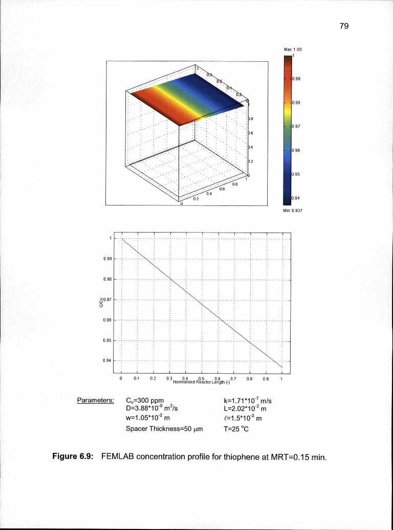
79

o go

o os

0.97C,

o 96

o 95

o 94

Max: 1 .00

96

95

Mm: 0.937

0 Dl 02 03 04 05 06 07 00 0.9Normalized Reactor Ler,th (-)

Parameters: C0=300 ppm k=1.71*107 m/sD=3.88*109 m2/s L=2.02*102 mw=1.05*102 m £=1.5*102 m

Spacer Thickness5O im 1=25 °C

Figure 6.9: FEMLAB concentration profile for thiophene at MRT=O.15 mm.

406

0.95

0.9

0,85

0.8

C-)

0,75

0.7

0.65

0.6

0.55

0.5

M 1 00

95

S

95

9

75

0.65

06

0.55

Mm; 0.521

0.1 0.2 0.3 0.4 0.5 0.6 0.7 0.8 0.9Normalized Reactor Length (-)

Parameters: C0=300 ppm k=1.71*107 rn/sD=3.88*109 m2/s L=2.02*102 mw=1.05*102 rn £=1.5*102 rn

Spacer Thickness=50 .tm T=25 °C

Figure 6.10: FEMLAB concentration profile for thiophene at MRT=1 .24 mm.

09

0.8

07

060

05

04

0.3

0.2

81

U 1110

08

817

IJ 8

0.4

.3

Mm: 0.208

I.....

H

0 0.1 0.2 0.3 0.4 0.5 0.6 0.7 0.8 0 9Normalized Reactor Length (-)

Parameters: C0300 ppm k=1.71*107 m/sD=3.88*109 m2/s L=2.02*102 mw=1.05*102 m £=1.51i2 m

Spacer Thickness=50 tm T=25 °C


0.9

0.8

07

0.6

0005

04

0.3

02

01

0.1 0.2 0.3 0.4 0.5 0.6 0.7 0.0 0.9Normalized Reactor Length (-)

Parameters: C0300 ppmD=3.88*109 m2/sw=1.05*102 m

Spacer Thickness=50 pm

k=1.71*107 rn/sL=2.02*102 m£=1.5*102 m

1=25 °C

Ma. 1 OIJ

S

8

7

6

4

2

Mm: 0.1 01


E*I

09

08

07

0.6

0.5

04

0,3

0.2

0.1

Max: 1 III

Mm: 0.0183

0 0.1 0.2 0.3 0.4 0.5 0.6 0.7 0.8 0.9Normalized Reactor Length (.)

Parameters: C0=300 ppm k=1.71*101 rn/sD=3.88*109 m2/s L=2.02*102 mw=1.05*102 m e=1.5*102 m

Spacer Thickness=50 jim 1=25 °C


84

1.0

0.8

0.60

C)C)

0.4

0.2

sI

NN NN

"\

NN- -

0.0 0.2 0.4 0.6 0.8 1.0


MRT = 0.15 mm.MRT=1.24min.MRT = 3.30 mm.- MRT = 4.79 mm.MRT=8.11 mm.

Parameters: C0=300 ppm k5.84*1 08 mis

D=3.88*109 m2/s L=2.02*102 mw=1.05*102 m £=1.5*102 mT=25 °C

Figure 6.14: FEMLAB concentration profile for thiophene at different meanresidence times, spacer thickness is 50 tm.

6.1.2 Desulphurization of Dibenzothiophene

Figure 6.15 represents the experimental and modeling results conducted

for dibenzothiophene desulfuraization with a spacer thickness of 100 tm and at

different mean residence times for the hexane layer inside the microreactor.

Again, it is also observed that the dibenzothiophene outlet concentration

decreased as the mean residence time inside the microreactor increased. This

reconfirmed our expectation that the dibenzothiophene conversion is strongly

dependent on the mean residence time. The results of the mathematical

modeling for a first order reaction fit well the experimental data. Once more,

these results confirm the assumption that the desulfurization of dibenzothiophene

fits first order reaction kinetics. The best value for the reaction rate constant (k) is

determined to be 1.47*10-7 m/s. This value is greater than that for the

desulfurization of thiophene; this indicates that dibenzothiophene is more

reactive than thiophene under the same reaction conditions.

1.0

0.8

0.6

000

0.4

0.2

0.0

0 2 4 6 8 10


Figure 6.15: Concentration of dibenzothiophene vs. mean residence time; modeland experiments. C0=300 ppm, L=2.20*102 m, w=1.05*1O2 m,spacer thickness is 100 jim, £=1 .5*102 m, T=25 °C.

The FEMLB modeling results for the desulfurization of dibenzothiophene

are shown if Figures 6.16 6.21. These figures are similar to those presented for

the thiophene. Each two plots represent the model results for a specific mean

residence time of reactants inside the microreactor, except Figure 6.21 which

shows the modeling results for all five different mean residence time cases.

0.998

0.996

0.994

S0992

0.99

0.988

0.986

0.984

87

1 L: LI

1

- U

0994

0.992

- 099

Mm: 0.984

9 0.1 0.2 °3NornézedR°ectorLi9th(-)°7 0.8 0.9 1

Parameters: C0=300 ppm k=6.50*108 rn/sD=3.45*109 m2/s L=2.02*102 mw=1 .05*1 02 m £1 5*102 mSpacer Thickness=1 00 pm 1=25 °C

Figure 6.16: FEMLAB concentration profile for dibenzothiophene at MRT=O.16mm.

[s.Is

Nax:1

LI

92

S

Mm: 0 885

0.98

0.96

0JO 94

0.92

0.9

0.880 0 1 0 2 0.3 0.4 0.5 0.6 0.7 0 8 0.9


Parameters: C0=300 ppm k=6.50*108 m/sD=3.45*109 m2/s L=2.02*102 mw1.05*102 m m

Spacer Thickness=1 00 pm T25 °C

Figure 6.17: FEMLAB concentration profile for dibenzothiophene at MRT=1 .25mm.

o 98

0 98

00 94

o 92

0.9

0 88

ylx I

0 0

8

IMm: 0.722

I

........................................................

..................... -1

0 0.1 0 2 0.3 0.4. 0.5 0.6 0.7 0.8 0.9Normalized Reactor Len9lIi (-)

Parameters: C0=300 ppm k=6.50*108 rn/sD=3.45*109 m2/s L=2.02*102 mw=1.05*102 m £=1.5*102 m

Spacer Thickness=1 00 J.Lm T=25 °C

Figure 6.18: FEMLAB concentration profile for dibenzothiophene at MRT=3.40mm.

0.95

0.9

0.85

0.800

0.75

0.7

0.65

0.6

0.55

0.50 0.1 0 2 0 3 0.4 0 5 0.6 0.7 0.8 0.9

Normalized Reactor LengTh (-)

Parameters: C0300 ppm k6.50*1 08 m/sD=3.45*109 m2/s L=2.02*102 mw=1.05*102 m £=1.5*102 m

Spacer Thicknessl 00 im T=25 °C

M: 1 00

96

9

85

65

Mm: 0.523


0.9

0.8

0.7

0.6

05

0&

91

Max: 1 Ii

Ii

0.7

IMm: 0.389

I

- .............................................. ,'.'. . .i ................................... -1

I I I I I I

0 01 0.2 03 04 05 06 07 08 0.9Normalized Reactor Length (-)

Parameters: C0=300 ppm k=6.50*106 rn/sD=3.45*1OO m2/s L2.02*102 mw=1.05*102 m £=1.5*102 m

Spacer Thickness=1 00 .tm T=25 °C


92

1.0

0.8

0.600

00.4

0.2

0.00.0 0.2 0.4 0.6 0.8 1.0


MRT = 0.16 mm.MRT=1.25min.MRT = 3.40 mm.- MRT = 6.59 mm.- - MRT 9.59 mm.

Parameters: C0=300 ppm k5.84*1 8mis

D=3.88*109 m2Is L=2.02*102 mw=1.05*102 m £=1.5*102 mT=25 °C

Figure 6.21: FEMLAB concentration profile for dibenzothiophene at differentmean residence times, spacer thickness is 100 jim.

93

6.2 Comparison between Thiophene and Dibenzothiophene

Both thiophene and dibenzothiophene were desulfurized under the same

experimental conditions in order to compare their reactivity in the photo

desulfuraization reaction in the presence of H202. Both reactions were found to

be much faster than expected when compared with available literature data.

Figure 6.22 shows the concentrations for the two compounds. It is evident from

this graph that dibenzothiophene is more reactive than thiophene and their

reaction rate constants are 1.47*10-7 m/s and 1.31*10-7 m/s, respectively. Brown

and Espenson [191 observed the same order of reactivity between thiophene and

di benzoth iophene.

1.0

0.8

0.60

C-)

C-,

0.4

0.2

0.00 2 4 6 8 10


Figure 6.22: Concentration profile of thiophene and dibenzothiophene vs. meanresidence time. C0300 ppm, L=2.20*102m, w1.05*102 m, spacerthickness is 100 .xm, £=1.5*102m, T=25 °C.

94

6.3 Effect of Spacer Thickness

Two experiments were conducted with thiophene under the same

experimental conditions with different spacer thicknesses. Changing the spacer

thickness also changes the mean residence time of the reactants inside the

microreactor.

Figure 6.23 indicates that when the spacer thickness is reduced, the outlet

concentration is smaller, i.e. better conversion is achieved. With 50 tm spacers,

the thickness of the hexane layer becomes smaller and therefore thiophene

takes less time to diffuse to the interface where the reaction occurs. As a result,

more thiophene molecules are desulfurized inside the microreactor. This also

contributes to the significantly different conversion. The value of the reaction rate

constant (k) value for the 50 .im case is 1.33*10-7 m/s, whereas the value of

1.31*1 o' rn/s is determined for the 100 tm case.

1.0

0.8

0.6

000

0.4

0.2

0.0

0 2 4 6 8 10


95

Figure 6.23: Concentration of thiophen vs. mean residence time for 50 .im and100 tm spacer thickness. C0=300 ppm, L=2.20*1 02 m, w=1.05*102m, t=1.5*102m, T=25°C.

6.4 Effect of UV source Distance

An investigation of the effect of the UV light intensity (from the mercury

lamp) was conducted by performing the experiments with the light source at

different distances from the microreactor (1 .5*1 02, 4.0*102, and 6.0*102 m). The

conversion vs. distance of the UV source () was presented in Figure 5.5 in

chapter 5. It was found that the distance substantially influences the conversion

of the thiophene.

As the light source distance from the microreactor increases, a lesser

amount of light is available to energize the reactants. Therefore, a lesser amount

of reactants are exited by the UV light which means that there are fewer amounts

of reactants available and ready for reaction to precede. As the distance between

the UV lamp and the microreactor decreases from 6.O*102 m to 1.5*102 m, the

conversion of thiophene increases by a factor of 1.94.

6.5 Comparison with Other Researchers' Work

In this section, we compare the performance results obtained in the

microreactor with the results obtained by other researchers. Figure 6.24

summarizes the results obtained by different authors. Results are presented for

both desulfurization of thiophene and dibenzothiophene. Curve number (1)

shows the concentration profile for the desulfurization of thiophene conducted in

a batch reactor with hydrogen peroxide but without UV light. It is clear that the

conversion for this process was very low considering the long time of reaction

(about 4 hours). Curve number (2) shows the concentration data obtained for

dibenzothiophene desulfurization with air bubbles and UV light. Although the

conversion for this process was high, it took a much longer time as compared to

the microreactor performance. The highest conversion for this process was

94.35% after ten hours of irradiation. Curve number (3) shows the concentration

profile for dibenzothiophene desulfurization with 30% hydrogen peroxide and UV

light at X > 280 nm. A conversion of 99% is achieved after 10 hours of irradiation.

97

Curve number (4) shows the concentration profile for dibenzothiophene

desulfurization with air bubbles and UV light. The conversion for this process was

96% after eight hours. Curve number (5) shows the concentration profile of 4,6-

DMDBT desulfurization with air bubbles and UV light. It is clear that a conversion

of about 80% was achieved after four hours of reaction. Curve number (6) shows

the dibenzothiophene concentration in a reaction with 30% hydrogen peroxide

and UV light. A conversion of 95% was obtained after four hours of irradiation.

Curve number (7) represents the microreactor result for thiophene desulfurization

conducted at 1OOtm. Curve number (8) represents the microreactor result for

thiophene desulfurization conducted at 5O.tm. Curve number (9) represents the

microreactor result for dibenzothiophene desulfurization conducted at 100.im.

It is evident from Figure 6.24 that the microreactor was much more

efficient for the desulfurization of thiophene and dibenzothiophene as was

anticipated due to understanding the advantages of microreactors. The

microreactor was capable of achieving 98.20% conversion at 8.11 mm. for

thiophene desulfurization.

1

0.8

0.6

000

0.4

0.2

0

0 100 200 300 400 500 600


o 1) Batch reactor I 7OoC [20]2) Batch reactor DBT no H202 air=0.5L/min 5OoC [23]

3) Batch reactor DBT 30% H202 50oC I>280nm [36]04) Batch reactor DBT no H202 air=1 L/min 5OoC [22]

5) Batch reactor 4,6-DMDBT no H202 air=1 L/min 5OoC [22]A 6) Batch reactor DBT 30% H202 500C [23]7) Microreactor T 100 mm8) Microreactor DBT 100 mm9) Microreactor - T - 50 mm

Figure 6.24: Comparison between microreactor's performance and batchreactor's performance.

CHAPTER 7CONCLUSION AND RECOMMENDATIONS

7.1 Conclusion

Desulfurization of thiophene and dibenzothiophene in the microreactor

was successfully investigated in this study. The microreactor used in the

experimental investigation contains spacers that have thicknesses of 5Opm and

100 pm as well as quartz windows. Two characteristic dimensions of the micro-

channel microreactor were used in this work: 50 pm and 100 pm. All

components of the microreactor were housed in a stainless steel casing. The

experiments were conducted at room temperature, 25°C. Different volumetric

flow rates of hexane (carrier fluid containing ppm quantities of thiophene and

dibezothiopene) corresponding to different residences were set in the range of

0.15 9.59 mm. A constant intensity UV light source was used to irradiate the

chemicals inside the microreactor through the quartz window. Samples were

collected and analyzed in the HPLC to determine the concentration of unreacted

thiophene or dibenzothiophene. A mathematical model that incorporates

convections, diffusion and chemical reaction was derived from the first principle.

The mathematical model was used to analyze (fit) experimental data, with the

chemical reaction rate constant as the only adjustable system parameter. In this

work we observed the effect of the micro-channel characteristic size (spacers'

thicknesses are proportional to the layers' thicknesses) and the effect of the

100

strength of the UV source on the conversion of thiophene and dibenzothiophene

in the microreactor. The comparison between microreactor performance and

batch reactor performance was studied in this work.

The UV light (254 nm) plays a major role in the desulfurization process of

thiophene and dibenzothiophene. Our experiments show that, in the absence of

UV light, no reaction takes place. This corroborates the suggested reaction

mechanism that the hydrogen peroxide molecule does not directly oxidize

thiophene and dibnezothiophene. Hydrogen peroxide degrades under UV light

and the products of this reaction help the photo-excited thiophene and

dibenzothiophene molecules to be oxidized. This was also observed in the study

conducted by T. Hirai [23].

Experiments show that the outlet concentration of thiophene and DBT

decreases as the mean residence time in the microreactor increases. This is

obvious because thiophene and dibenzothiophene remain longer in the reactor

and thus their conversion increases with time.

In this study we also proposed a mathematical model for the microreactor

chemical process whose main features are convection, axial and radial diffusion,

and heterogeneous chemical reaction at the interface between the two

immiscible streams. Pertinent boundary conditions were proposed for the

mathematical model of the microreactor. A numerical solution using FEMLAB

101

(modeling software) was successfully implemented and presented in this work.

The results of the mathematical modeling for the first order oxidative

desulphurization reaction for thiophene and dibenzothiophene correspond well to

the experimental data. As a result of the modeling, the reaction rate constant (k)

was determined and found to be of the order of I o' (mis) for both thiophene and

dibenzothiophene desulfurization.

When this result is compared to reaction rate constants reported by other

investigators we find that this reaction proceeds much slower in a batch reactor

than in the microreactor. For example, Brown [19] reported a value of k = 2.7*104

(s1) for thiophene desulfurization; Gvozdetskaya [20] reported a value of k =

1.67*104 (1) also for thiophene desulfurization. For the desulfurization of

dibenzothiophene, Hirai [22] reported a value of k= 3.81*10.4 (molim3.$), and

Shiraishi [24] reported a value of k = 2.86*10.5 (s1). Table 7.1 compares basic

information related to the results of this study and to the information found in

open literature.

102

Table 7.1: Basic information related to the results of this study and information found in open literature.

AuthorReference

Desulfurization ofThioDhene/DBT used

Oxidantused

UV light]Catalyst

Reported reactionrate constant

Pseudo first orderreaction rate constant

Reactortvoe

Brown [19] Thiophene 30% H202 Catalyst 2.7*1 0 S1 2.7*1 4 -i Batch-reactor

Gvozdetskaya [20] Thiophene 30% H202 HCI 1.67*1 0s_i 1.67*1 0 Batch-reactor

This work Thiophene 30% H202 ?=254 nm 1.31*10-7 ms1 1.44*10-3 s microreactor

Hirai [22] DBT 30% H202 ?<280 nm 3.81 *1 O mol/m3.s 3.50*10-5 s_i Batch-reactor

Shiraishi [24] DBT 30% H202 ?.<280 nm 2.86*10-5 s_i 2.86*105 s' Batch-reactor

This work DBT 30% H202 X=254 nm 1.47*10-7 ms 1 .61*10 s' microreactor

103

In this study both thiophene and dibenzothiophene were tested under the

same experimental conditions to compare their reactivity in the microreactor. We

found that dibenzothiophene is slightly more reactive than thiophene and that the

reaction rate constants for thiophene and dibenzothiophene are 1.31*10-7 m/s

and 1.47*1 0 m/s, respectively. Similar reactivities were observed by Brown and

Espenson when they compared conversions of thiophene and dibenzothiophene

[191.

The reduction in the spacer thickness of the microreactor results in better

reactor performance, i.e. faster reaction process. Decreasing the spacer

thickness helps by reducing the diffusion path length for the thiophene to the

reaction interface, and thus it accelerates the overall reaction process. The

reduction of the reactor thickness obviously improves the mass transfer operation

and enhances he overall process performance.

In this study we also investigated how the change in the distance between

the UV lamp and the microreactor influences the conversion of the thiophene.

The change in the distance of the UV source from the reactor quartz window

changes the flux of the light, which, in turn, changes the rate of the reaction

process. When the distance between the UV lamp and the microreactor is

increased, the rate of the desulfurization process decreases. As the distance of

the light source increases from the microreactor, less amount of light is available

to energize the reactants in the microreactor. Therefore, a lesser amount of

104

reactants are excited by the UV light, which means that fewer reactant molecules

are available and ready for reaction to proceed.

The experimental results obtained form the microreactor study were

compared with the work reported by other researchers in this field. We find that

the microreactor is much more efficient than batch reactors for the desulfurization

process of thiophene and dibenzothiophene. This is an anticipated outcome

based on the understanding of the advantages of microreactors in performing

reaction processes in which mass transfer components play important role. In

this study the microreactor was capable of achieving a 98.2% conversion of

thiophene in approximately 9 (mm.) which compares to 240-600 (mm.) for a

macroscopic batch reactor operation.

In summary, we have shown that the desulfurization of thiophene and

dibenzothiophene can be achieved in a microreactor by contacting the

thiophenes and hydrogen peroxide under UV irradiation at room temperature.

The mathematical models proposed, along with the corresponding numerical

solutions obtained, were accurate enough to extract the pseudo first order

reaction rate constant and to predict the concentration profile of the reactant in

the microreactor.

105

7.2 Recommendations

All experimental data presented in this study were obtained at a room

temperature of 25°C. Faster process rates are expected at higher reaction

temperatures, therefore an investigation of desulfurization reactions in

microreactors at temperatures up to approximately 70 °C is worth examining.

Increased reaction temperatures will demand different construction materials and

as well as a different microreactor design. Besides focusing on materials used

and on the heat source for the high temperature experimental apparatus, it would

be beneficial to seek catalysts for this reaction process. The UV sources may be

cumbersome to implement in high temperature operations. It may be necessary

to replace the UV radiation with an appropriate catalyst. There are two main

catalysts used for selective desulfurization of thiophenes: organic acids and

polyoxometalates (POM). Organic acids include formic acid, acetic acid, citric

acid, carbonic acid, and hydrogen cyanide. POM have long been studied for

oxidation reactions, particularly the POM/hydrogen peroxide system for organic

substrate oxidations.

Optimization of the consumption of hydrogen peroxide in this reaction

process is another area that needs to be explored. The ratio of the H2O2 to

hexane used in this study can be reduced and H202 solutions with concentrations

of 6% and 3% can be implemented.

106

Further reduction of the reactor thickness can be implemented as well. We

were able to achieve over a 98% conversion in a 50 tm microchannel reactor,

and it is logical to explore how a smaller microchannel (25 pm for example)

would influence the rate of the reaction process.

Real logistic fuels, like gasoline and diesel, could be introduced into the

microreactor to find how efficient this process is under conditions of a real

application. Special care would need to be devoted to the analytical technique in

order to positively and easily recognize all participants in the reaction with real

logistic fuels.

UV light plays a major role in the desulfurization process. UV lamps are

available at different wavelengths. Therefore, a UV lamp with a shorter

wavelength can be examined to determine what level of process rate

improvement one can expect from this application.

Previous studies [22,23] show that the desulfurization can be accelerated

by introducing oxygen bubbles into the reaction mixture. This approach the use

of gaseous oxidants can have important consequences in the design of a

microreactor for the gas-liquid reaction process.

There are large varieties of extraction solvents that can be implemented in

the desulfurization of fuels. Water was used in this study as a polar extraction

107

solvent and as a hydrogen peroxide carrier fluid. Another type of extraction

solvent, like ionic fluids, could be used in this study as some of these solvents

can extract more of the undesired chemicals from obtained reaction products.

This would give a higher quality product.

BIBLIOGRAPHY

I OSHA Technical Manual, Section IV, Chapter 2, http:I/www.osha.qov

2 Z. C. Mester, "Meeting Sulfur Specifications for 2000 and Beyond", March2000, http://www.environmentalconsultation.com/sulfEnq.html

3 World-Wide Fuel Charter, December, 2002

4 Diesel Fuel News, May 10, 1999

5 Control of Air Pollution from New Motor Vehicles: Heavy-Duty Engine andVehicle Standards and Highway Diesel Fuel Sulfur Control Requirements,EPA, January 18, 2001

6 Final Report of the Government Working Group on Sulfur in Gasoline andDiesel Fuel, January, 2005)

7 Tushingham, M.,Regional Composition of Gasoline and Diesel, October,1996

8 Dieselnet, July 30, 1999

9 Conservation of Clean Air and Water in Europe (CONCAWE), Report No.6/97

10 Conservation of Clean Air and Water in Europe (CONCAWE), V5, No 1,April 1996

11 Walsh, M., Shah, J. Clean Fuels for Asia, World Bank Paper No. 377, 1997

12 Octane Week, October 26,1998

13 E.R. Deisman, E.V. Rebrov, M.H.J.M. de Croon, J.C. Schouten, G.J.Kramer, V. Cominos, T.. Richter, T.T. Veenstra, A. van den Berg, P.D.Cobden, F.A. de Bruijn, C. Ferret, U. d' Ortona, L. Falk, Micro reactortechnology for hydrogen and electricity, in Proc. 5th mt. Conf. onMicroreaction Technology (IM RET5), ISBN 3-540-42489-9, SpringerVerlag, Berlin; Editors: M. Matlosz, W. Ehrfeld, J.P. Baselt, Strasbourg,France, 368-374, (2001).

14 W. Ehrfeld, V. Hessel, H.Lehr, "Microreactors for chemical synthesis andbiotechnology current developments and future applications" in:Microsystem technology in chemistry and life science, 1998, pp. 233-252.

109

BIBLIOGRAPHY (continued)

15 Kleemann, A., "Microreaction Technology Applications In PharmaceuticalResearch, Development and Production", Innovations in PharmaceuticalTechnology, September 2001

16 Wille, C., Autze, V., Kim, H., Nickel, U., Oberbeck, S., Schwalbe, T.,Unverdorben, T., "Progress in Transferring Microreactors from Lab intoProduction-an Example in the Field of Pigments Technology", IMRET 6 - 6thInternational Conference on Microreaction Technology, 2002,

17 Hessel, V., Eherfeld, W., Golbig, K., Haverkamp, V., Lowe, H., Storz, M.,Wille, C., Jahnisch, K., Baerns, M., "Gas/liquid microreactors for directflourination of aromatic compounds using elemental flourine", in Ehrfeld, W.(Ed.), Microreaction Technology: 3rd International Conference onMicroreaction Technology, Proceedings of IMRET 3, 2000, 526-540

18 Krummradt, H., Kopp, U., Stoldt, J., "Experiences with the use ofmicroreactors in organic synthesis",in Ehrfeld, W. (Ed.), MicroreactionTechnology: 3rd International Conference on Microreaction Technology,Proceedings of IMRET3, 2000, 181-1 86

19 Kylie N. Brown and James H. Espenson, "Stepwise Oxidation of Thiopheneand Its Derivatives by Hydrogen Peroxide catalyzed byMethyltrioxorhenium (VII)", lnorg. Chem. 1996, 35, 7211-7216

20 V. P. Gvozdetskaya, "Oxidation of Thiophene by Hydrogen Peroxide"Zhurnal Prikladnoi Khimii, 1977, 50, 4, 900-903

21 Resat Apak and Mehmet Hugul, "Photooxidation of Some Mono-, Di-, andTri-chiorophenols in Aqueous Solution by Hydrogen Peroxide/UVCombinations", J. Chem. Tech. Biotechnol., 1996, 67, 221-226

22 T. Hirai, K. Ogawa, and I. Komasawa, "Desulfurization Process forDibenzothiophenes from Light Oil by Photochemical Reaction and Liquid-Liquid Extraction", Ind. Eng. Chem. Res., 1996, 35, 586-589

23 T. Hirai, K. Ogawa, Y. Shiraishi, and I. Komasawa, "Effect ofPhotosensitizer and Hydrogen Peroxide on Desulfurization of Light Oil byPhotochemical Reaction and Liquid-Liquid Extraction", Ind. Eng. Chem.Res., 1997, 36, 530-533

110


24 Y. Shiraishi, K. Tachibana, T. Hirai, and I. Komasawa, "Desulfurization andDenitrogenation Process for Light Oils Based on Chemical Oxidationfollowed by Liquid-Liquid AExtraction", Ind. Eng. Chem. Res., 2002, 41,4362-4375

25 Bielski, B. H. J. & Cabelli, D. E., Highlights of current research involvingsuperoxide and perhydroxyle radicals in aqueous solutions (Review), mt. J.Radiat. Biol., 59 (1991) 291-319

26 Glaze, W. H., Kang, J. W. & Chapin, D. H., The chemistry of watertreatment processes involving ozone. Science and Engineering, 9 (1987)335-52

27 Baxendale, J. H., The photolysis of hydrogen peroxide at high lightintensities. Trans. Faraday Soc., 53 (1957) 344-56

28 Fox, M. A. & Chen, C. C., Mechanistic features of the semiconductorcatalyzed olefin-to-carbonyl oxidative cleavage, J. Am. Chem. Soc., 103(1981) 6757

29 011is, D. F., In Homogeneous and Heterogeneous Photocatalysis, eds E.Pelizzetti & N. Serpone, Reidel, Dordrecht, The Netherland, 1986, p.651

30 Barbeni, M., Minero, C., Pelizzetti, E., Borgarello, E., Serpone, Chemicalderadation of chlorophenols with Fenton's reagent (Fe2 + H202), N.Chemosphere, 16 (1988) 2225

31 Arantegui, J., Prado, J., Chamarro, E. & Esplugas, S., Kinetics of the UVdegradation of atrazine in aqueous solution in the presence of hydrogenperoxide, J. Photochem. Photobiol. A: Chemistyr, 88 (1995) 65-74

32 B. Grieb, "Green Oxidation of Thiophenes",http://students.cntre.edu/bcqrie00/abstractNCUR.html

33 F. M. White, "Fluid Mechanics", 2nd edition, McGraw-Hill, Inc., 1986

34 R. Glimont, "Liquid Viscosity Correlations for Flowmeter Calculations",CEP, October 2002, 36-41

35 "Dynamic, Absolute, and Kinematic Viscosity", Fluid Mechanics, TheEngineering Toolbox, http://www.engineerinptoolbox.com

111


36 Y. Shiraishi, H. Hara, T. Hirai, I. Komasawa, "A Deep DesulfurizationProcess for Light Oil by Photosensitizer Oxidation Using a TripletPhotosensitizer and Hydrogen Peroxide in an Oil/Water Two-Phase Liquid-Liquid Extraction System", Ind. Eng. Chem. Res., 1999, 38, 1589-1 595

37 5. Middleman, "An Introduction to Mass and Heat Transfer: Principles ofAnalysis and Design", 1997

38 F. M. White, "Viscous Fluid Flow", McGraw-Hill, Inc., 1991, 121-123

39 R. K. Shah, and A. L. London, "Laminar Flow Forced Convection in Ducts",Academic, New York, 1978

40 0. Joshi, "Fibrinogen adsorption at heparinized silica interfaces: Historydependence and protein concentration effects", 2004

41 W. Lee, "Kinetic modeling of the adsorption of structural stability mutants ofbacteriophage T4 lysozyme at solid-water interfaces", 1999

42 Levine, Ramsey, Smidt, "Applied statistics for engineers and scientists:Using Microsoft Excel & Minitab: lie", Prentice Hall, 2001, 427-431

43 J. Sedlbauer et al., "Group Contribution Method for the Henry's LawConstant of Aqueous Hydrocarbons",http://www.fp.vslib.cz/kcWsedlbauer/AicheAll .pdf

112

APPENDICES

113

APPENDIX ACALCULATION OF THE RATIO OF LAYERS THICKNESSES

Equation (3.15) in chapter 3is solved for the ration of the layer thicknesses

(B). The left hand side of equation (3.15) is set equals to one because the two

fluids are delivered by the syringe pump which has the same syringes size for

both fluids (10 mL syringes). Equation (3.15) is solved by trial and error suing

spread sheets as follows:

= I = B

i+__1B26t BIA+B2A\B-f-1) 3AB+1

i_!_1B2 IIA-1-B2BB+1) 3BB+1

A =3.3*10 Pa.s = 0.367

b9.0*104 Pa.s

(3.15)

The spread sheet output in Table A.1 revealed that the value of which sets

the ratio of the two fluids volumetric flow rate equals one is:

B = Ba/Bb = 0.84

114

Table A.1: Calculations of the ratio of the layers thicknesses.

AssumedB QaIQb Assumed

B QaIQb AssumedB QaIQb Assumed

B QaIQb

0.700 0.754 0.740 0.821 0.780 0.891 0.820 0.9630.701 0.756 0.741 0.823 0.781 0.893 0.821 0.9650.702 0.757 0.742 0.825 0.782 0.895 0.822 0.9670.703 0.759 0.743 0.826 0.783 0.896 0.823 0.9690.704 0.761 0.744 0.828 0.784 0.898 0.824 0.9710.705 0.762 0.745 0.830 0.785 0.900 0.825 0.9720.706 0.764 0.746 0.832 0.786 0.902 0.826 0.9740.707 0.766 0.747 0.833 0.787 0.903 0.827 0.9760.708 0.767 0.748 0.835 0.788 0.905 0.828 0.9780.709 0.769 0.749 0.837 0.789 0.907 0.829 0.9800.710 0.771 0.750 0.839 0.790 0.909 0.830 0.9820.711 0.772 0.751 0.840 0.791 0.911 0.831 0.9840.712 0.774 0.752 0.842 0.792 0.912 0.832 0.9850.713 0.776 0.753 0.844 0.793 0.914 0.833 0.9870.714 0.777 0.754 0.845 0.794 0.916 0.834 0.9890.715 0.779 0.755 0.847 0.795 0.918 0.835 0.9910.716 0.781 0.756 0.849 0.796 0.920 0.836 0.9930.717 0.782 0.757 0.851 0.797 0.921 0.837 0.9950.718 0.784 0.758 0.852 0.798 0.923 0.838 0.9970.719 0.786 0.759 0.854 0.799 0.925 0.839 0.9980.720 0.787 0.760 0.856 0.800 0.927 0.840 1.0000.721 0.789 0.761 0.858 0.801 0.929 0.841 1.0020.722 0.791 0.762 0.859 0.802 0.930 0.842 1.0040.723 0.792 0.763 0.861 0.803 0.932 0.843 1.0060.724 0.794 0.764 0.863 0.804 0.934 0.844 1.0080.725 0.796 0.765 0.865 0.805 0.9360.726 0.798 0.766 0.866 0.806 0.9380.727 0.799 0.767 0.868 0.807 0.9390.728 0.801 0.768 0.870 0.808 0.9410.729 0.803 0.769 0.872 0.809 0.9430.730 0.804 0.770 0.873 0.810 0.9450.731 0.806 0.771 0.875 0.811 0.9470.732 0.808 0.772 0.877 0.812 0.9490.733 0.809 0.773 0.879 0.813 0.9500.734 0.811 0.774 0.880 0.814 0.9520.735 0.813 0.775 0.882 0.815 0.9540.736 0.814 0.776 0.884 0.816 0.9560.737 0.816 0.777 0.886 0.817 0.9580.738 0.818 0.778 0.887 0.818 0.9600.739 0.820 0.779 0.889 0.819 0.961

115

APPENDIX BCALCULATION OF PRESSURE DROP AND RESIDENCE TIME

The pressure drop (AP) inside the microreactor is determined by equation

(3.21) in chapter 3.

AP2

bL

a(A+B) (3.21)

B Ba2 (A+BlBaBbW(B+1)[ a 2AB+1J 3ABbB+1J]

The mean residence time (MRT) of reactants inside the microreactor is

determined according to the following equation:

MRT=--

where MRT = Residence time (s)

= Volumetric flow rate of the hexane (m3/s)

Va = Volume of the hexane layer inside microreactor, top layer (m3)

The calculations are conducted at different flow rates for two cases. In the

first case, the microreactor had two spacers each one is having 100 jim

thickness. In the second case, the microreactor had two spacers each one is

having 50 jim thickness. The results are presented in Table B.1 and Table B.2.

116

Table B.1: Pressure drop and mean residence time calculations using 2spacers each of 100 .tm thickness.

Syringe PumpSetting

Qa Rated(cm3/min)

Qa Actual(cm3/min) AP (Pa) MRT (mm.)

14 0.1354 0.1348 3.50 0.1616 0.0704 0.0700 1.82 0.3020 0.0176 0.0169 0.44 1.2522 0.0093 0.0085 0.22 2.4823 0.0066 0.0062 0.16 3.4024 0.0047 0.0042 0.11 5.0225 0.0034 0.0032 0.08 6.5926 0.0024 0.0022 0.06 9.5928 0.0012 0.0013 0.03 16.22

Table B.2: Pressure drop and mean residence time calculations using 2spacers each of 50 tm thickness.

Syringe Pump ilSetting j

Qa Rated(cm3/min)

Qa Actual(cm3/min)

1

j

AP(Pa)1

MRT (mm.)

14 0.1354 0.1348 28.00 0.0816 0.0704 0.0700 14.54 0.1520 0.0176 0.0169 3.51 0.6222 0.0093 0.0085 1.77 1.2423 0.0066 0.0062 1.29 1.7024 0.0047 0.0042 0.87 2.5125 0.0034 0.0032 0.66 3.3026 0.0024 0.0022 0.46 4.7928 0.0012 0.0013 0.27 8.11

117

APPENDIX CPROCEDURE OF THE WINDOWS CHEMICAL TREATMENT

The following procedure was followed to prepare the hydrophilic andhydrophobic quartz windows [40,41].

Prior Preparation:

1. Set water bath at 80 °C and turn on 1-2 hrs before.

2. Rinse window with acetone.

3. Prepare I % silanizing solution by adding 100 p1 dichlorodimethylsilane in10 ml xylene.

4. Prepare acid/base cleaning solutions.

Step I Hydrophilic window

1. Place quartz window into a mixture of NH4OH:H202:H20 (1:1:5 volume

ratio), then heat for 10 mm at 80 °C in a water bath.

2. Rinse with copious amount of distilled, deionized water.

3. Place the window into a mixture of HCI:H202:H20 (1:1:5 volume ratio),

then heat for 10 mm at 80 °C in a water.

4. Rinse with distilled, deionized water, and store in 100% ethanol untilneeded.

Step 2 Hydrophobic window

1. After having rinsed with distilled, deionized water, dry window with N2,then place into an 1% solution of dichlorodimethylsilane (in xylene) for I h.

2. Rinse with about 100 ml each of xylene, acetone, then ethanol, and then

store in 100% ethanol until needed

118

APPENDIX DSTANDARD CURVES FOR THIOPHENE AND DIBENZOTHIOPHENE

A series of known concentrations at 20 ppm, 50 ppm, 100 ppm, 200 ppm,

and 300 ppm of both thiophen and dibenzothiophen were prepared in hexane

and thoroughly mixed. These solutions were individually injected into the HPLC

column. The Waters XTerra RPI8 column is 3.5tm 4.6x150 mm (particle size,

column ID, and column length with pore size of 125 A°, respectively). The sample

injection volume was 20 jiL. Dibenzothiopheen was diluted by a factor of 1.7 due

to peak size limitations in the HPLC. Mobile phase which consists of 65%

Acetonitrile, 5% Tetrahydrofuran, and 30% buffer soulution (pH=3.0, 25mM

monobasic sodium phosphate titrated with phosphoric acid) were used in the

analysis.

The series of solution peaks areas were recorded by Visual Designer

software and plotted against the solution concentrations. A sample

chromatograph for the analysis of thiophene and dibenzothiophene were plotted

in Chapter 4. Standard curves for peak area vs. concentration (ppm) for both

thiophene and dibenzothiophene were also obtained and shown in Figure Di

and D.2, respectively, for later use in determining product solutions

concentrations.

160x103

140x 10

120x103

100x103

80x103

60x103

40x103

20x103

0 r0 50 100 150 200 250 300 350

Thiophene Concentration (ppm)

Figure D.1: Standard curve for HPLC analysis of thiophene concentrations atUV detector wavelength of 254 nm.

1 2x106

10x106

8x106

6x106

4x106

2x106

0 r I I I I

0 50 100 150 200 250 300 350

Dibenzothiophene Concentration (ppm)

Figure D.2: Standard curve for HPLC analysis of dibenzothiopheneconcentrations at UV detector wavelength of 254 nm.

120

APPENDIX EEXPERIMENTAL DATA

Thedesulfurization experiments are conducted for two sulfur containing

compounds, thiophene and dibenzothiophene. The parameters that has been

changed in every set of experiments are:

. The sulfur compound used (thiophene, and dibenzothiophene)

. The spacer thickness (50, and 100 jim)

. The distance of the UV light source (0.5, 3.0, and 5.0 cm)

For every set of experiments, the mean residence time inside the

microreactor is being varied to get a number of points that is enough to make it

reasonable for conducting results analysis. All sets of experiments data are

tabulated in Tables E.1 E.4.

121

Table E.1: Experimental data for thiophene desulfurization. C0=300 ppm, L=2.20*102 m, w=1.05*102 m, spacerthickness is 100 tm, £=1 .5*1 02 m, T=25 °C.

Sample MRT Peak tR Height Area Concentration(mm.) (mm.) (Millivolts) (Millivolts*min.) (ppm)

Feed 0.00 2.30 11,096.05 135,840.00 300.00Feed 0.00 2.30 11,712.35 137,277.00 300.00Feed 0.00 2.30 11,567.79 135,295.00 300.00Product 0.16 2.29 9,854.46 127,801.00 286.31Product 0.16 2.30 9,969.73 123,894.00 277.55Product 0.16 2.30 9,790.40 126,059.00 282.40Product 1.25 2.29 9,502.21 118,586.00 265.66Product 1.25 2.30 9,474.15 120,885.00 270.81Product 1.25 2.29 9,808.68 120,856.00 270.75Product 3.40 2.29 7,537.68 100,509.00 225.16Product 3.40 2.30 7,095.46 97,806.00 219.11Product 3.40 2.30 6,996.42 102,584.00 229.81Product 6.59 2.30 7,608.87 73,845.00 165.43Product 6.59 2.30 7,545.60 71,815.00 160.88Product 6.59 2.33 7,210.07 70,567.00 158.09Product 9.59 2.33 4,829.65 58,486.00 131.02Product 9.59 2.34 5,057.12 62,836.00 140.77Product 9.59 2.33 5,397.39 61,626.00 138.06

122

Table E.2: Experimental data for thiophene desulfurization. C0=300 ppm, L=2.20*102 m, w=1.05*102 m, spacerthickness is 50 pm, £=1 .5*1 02 m, T=25 °C.

Sample MRT T Peak tR Height Area Concentration(mm.) (mm.) (Millivolts) (Millivolts*min.) (ppm)

Feed 0.00 2.30 11,096.05 135,840.00 300.00Feed 0.00 2.30 11,712.35 137,277.00 300.00Feed 0.00 2.30 11,567.79 135,295.00 300.00Product 0.15 2.32 7,908.61 115,196.00 258.07Product 0.15 2.33 7,930.73 110,492.00 247.53Product 0.15 2.33 8,277.18 115,534.00 258.82Product 1.24 2.33 3,673.49 71,336.00 159.81Product 1.24 2.35 3,371.14 69,824.00 156.42Product 1.24 2.34 3,085.04 69,472.00 155.63Product 3.30 2.33 2,869.39 28,807.00 64.53Product 3.30 2.34 2,930.39 30,138.00 67.52Product 3.30 2.35 2,854.99 28,027.00 62.79Product 4.79 2.34 421.72 13,815.00 30.95Product 4.79 2.34 409.82 14,719.00 32.97Product 4.79 2.34 409.84 14,229.00 31.88Droduct 8.11 2.34 309.85 2,494.00 5.59Product 8.11 2.35 210.51 2,243.00 5.02Product 8.11 2.34 203.26 2,391.00 5.36

123

Table E.3: Experimental data for thiophene desulfurization for the effect of UV source distance. C0=300 ppm, L=2.20*102m, w=1.05*102 m, spacerthickness is 100 jtm, MRT=6.59 mm, T=25 °C.

Distance of UV Source Sample Peak tR Height Area Concentration(cm) (mm.) (Millivolts) (Millivolts*min.) (ppm)

2.30 11,458.73 136,137.33 300.00Feed 2.30 11,458.73 136,137.33 300.00

2.30 11,458.73 136,137.33 300.002.29 21,297.20 101,990.00 224.75

6.0 Product 2.29 21,278.76 103,367.00 227.792.27 21,264.08 104,020.00 229.222.29 8,269.96 94,070.00 207.30

4.0 Product 2.28 7,452.87 95,665.00 210.812.29 8,329.26 96,206.00 212.012.30 7,608.87 73,845.00 162.73

1.5 Product 2.30 7,545.60 71,815.00 158.262.33 7,210.07 70,567.00 155.51

124

Table E.4: Experimental data for dibenzothiophene desulfurization. C0=300 ppm, L=2.20*1 02 m, w=1.05*102 m, spacerthickness is 100 jim, £=1 .5'1 02 m, T=25 °C.

Sample MRT Peak tR Height Area Concentration(mm.) (mm.) (Millivolts) (Millivolts*min.) (ppm)

Feed 0.00 4.14 858,799.06 10,075,935.00 300.00Feed 0.00 4.14 878,280.69 10,203,764.00 300.00Feed 0.00 4.15 914,727.44 10,248,184.00 300.00Product 0.16 4.15 910,850.38 9,521,424.00 279.33Product 0.16 4.15 923,455.94 9,684,753.00 284.12Product 0.16 4.12 852,903.94 8,951,548.00 262.61Product 1.25 4.13 844,639.69 8,902,133.00 261.16Product 1.25 4.14 828,390.19 8,734,986.00 256.25Product 1.25 4.14 789,403.75 8,361,249.00 245.29Product 3.40 4.14 756,637.75 8,065,891.00 236.62Product 3.40 4.13 750,018.88 8,363,600.00 245.36Product 3.40 4.13 759,580.81 8,145,711.00 238.97

roduct 6.59 4.08 502,260.28 4,954,191.00 145.34Product 6.59 4.06 528,099.00 5,342,645.00 156.73Product 6.59 4.08 473,938.91 4,762,706.00 139.72Product 9.59 4.11 435,898.38 4,460,858.00 130.87Product 9.59 4.11 421,329.34 4,509,828.00 132.30Product 9.59 4.12 431,720.69 4,484,875.00 131.57

125

APPENDIX FOPTIMIZATION FOR REACTION RATE CONSTANT (k)

An optimization procedure implemented to search for the best value for

the reaction rate constant (k) that makes the mathematical model fits with the

experimental points. The search is done until the objective function (OF) as

expressed by equation F.1 reached a minimum.

5

OF = [(Cn/Co)expt (Cn/Co)modeIl2 F.1n=1

The model output as compared to the experimental data was then

graphed for a variety of reaction rate constants as shown in Figures F.1 F.3. As

it's known from a mathematical perspective, the least three points around the

minimum point are forming a quadratic function in the following general form:

f(x) Qo + Qi X + Q2 F.2

From Figures F.1, F.2, and F.3, the corresponding quadratic equations are

having the flowing forms:

Thiophene, Spacer thickness = 100 .im

OF = 0.305 4598980.696 k + 1.753*10+13 k 2 F.3

126

Thiophene, Spacer thickness = 50 jim

OF = 0.312-4560771.863 k + 1.709*10*13 k2 F.4

Dibenzothiophene, Spacer thickness = 100 jim

OF = 0.304 3993797.748 k + 1.356*10+13 k 2 F.5

Equations F.3 F.5 are solved for (k) by taking the first derivative and

equating to zero to get the minimum value for the objective function. The

solutions reveal the following results:

k = 1.31*10-7 m/s (Thiophene, Spacer thickness = 100 jim)

k = I .33*107 rn/s (Thiophene, Spacer thickness = 50 jim)

k = 1.47*1 O m/s (Dibenzothiophene, Spacer thickness = 100 jim)

6.00e-3

5.50e-3

C5.00e-3

UC

4.50e-3

4.00e-3

0

3.50e-3

3.00e-31

1.15e-7 1.20e-7 1.25e-7 1.30e-7 1.35e-7 1.40e-7 1.45e-7

k (mis)

Figure F.1: Objective function vs. k for thiophene at spacer thickness of 100jim.

127

1.15e-2

1.lOe-2

1.05e-20

1 .00e-2

9.50e-3

9.00e-3

0 8.50e-3

8.00e-3

7.50e-3!

1.1 5e-7 1 .20e-7 1 .25e-7 1 .30e-7 1 .35e-7 1 .40e-7 1 .45e-7

k (mis)

Figure F.2: Objective function vs. k for thiophene at spacer thickness of 50 jim.

1 .20e-2

1.1 5e-2

2 1.lOe-2UC

1.05e-2

:i 1 .00e-2

0

9.50e-3

9.00e-31

1 .35e-7 1 .40e-7 1 .45e-7 1 .50e-7 1 .55e-7 1 .60e-7 1 .65e-7

k (mis)

Figure F.3: Objective function vs. k for dibenzothiophene at spacer thickness of100 jim.

128

APPENDIX GCALCULATION OF THIOPHENE AND DIBENZOTHIOPHENE DIFFUSIVITIES

An estimation of diffusivities of non-electrolytes in liquids at low

concentration is given byWilke and Chang, 1955 [37]:

(c1 MWB)112TDAB =7.4*108

PB V°6

Where, DAB = Diffusivity of solute at infinite dilution (cm2/sec)

= Association parameter (hexane=1)

M W,B = Solvent molecular weight (g/mol)

T = Absolute temperature (K)

PB Solution viscosity (centipoises)

VA = Molar volume of solute at normal boiling point (cm3/mol)

Diffusivity of Thiophene in Hexane:

(G.1)

DAB = 7.4 * I O8(1 * 84.15)1/2(298) = 3.88 *105cm2/sec 3.88*109m2/sec

(O.33)(99.6)06

Diffusivity of Dibenzothiophene in Hexane:

DAB =7.4*108 (1*184.27)1/2(298)= 3.45 *105cm2/sec = 3.45*1O9m2/sec

(O.33)(232.8)06

129

APPENDIX H CALCULATION OF REYNOLDS NUMBER

The Reynolds number (Re) can be calculated from equation HA. [38]:

Re= PUavg Dh

(H.1)

Where, p = Fluid density (kg/rn3)

Uavg = Fluid average velocity (mis)

Dh = Hydraulic diameter (m) = [4*(W*Ba)] / [2(W+Ba)]

= Fluid viscosity (Pa.$)

Table H.1: Calculation of Re

Parameter Spacer Thickness =100 tm Spacer Thickness = 50 tm

Lowest Flow Highest Flow Lowest Flow Highest Flow p 659 659 659 659

Uavq 3.82*10-5 2.34*1O 4.52*105 2.43*10 Dh 1 81*10-4 1 81*10-4 9 10*10-5 9 io*io

lL 33*104 3.3*10-4 33*104 33*104

Re 0.014 0.846 0.008 0.442

130

APPENDIX ICALCULATION OF ENTRANCE LENGTH

To insure that we have fully developed laminar flow inside the

microreactor reaction region it is required to calculate the entrance length for fully

developed velocity profile. The entrance length can be calculated from equation

1.1 [38].

0.6 +0.056Re 1.1Dh I + 0.035 Re

Where, Re = Reynolds number

Dh = Hydraulic diameter (m) = [4*(W*Ba)] / [2(W+Ba)]

x L = Entrance length (m)

By utilizing the Reynolds number data from Table H.1, The results for the

entrance length are presented in Table 1.1.

Table II: Calculation of entrance length (x L).

Parameter Spacer Thickness =100 tm Spacer Thickness = 50 jm

Lowest Flow Highest Flow Lowest Flow Highest FlowDh 1.81*10-4 1.81*10-4 9.1O*105 9.10*10Re 0.014 0.846 0.008 0.442XL 1.09*104 1.14*10-4 0.55*10-4 0.56*10-4

131

APPENDIX JHYPOTHESIS TESTING FOR PAIRED DATA

The t-test statistic for the mean difference for the experimental data

obtained for thiophene and dibenzothiophene is done to determine whether the

two sets of data are statistically different [42]. The following equations are used:

= (J.1)SD

D = (J.2)n

/(D1 - D)2

SD'=

n-i (J.3)

For a given level of significance, a, we reject the null hypothesis (H0) if the

computed t-test statistic exceeds the upper-tailed critical value tn_I from the t

distribution or if the computed test statistic falls below the lower-tailed critical

value tnl from the t distribution. That is, the decision rule is:

Reject H0 if t> tn_I

or if t > tn-I

Otherwise do not reject H0,

132

Where, t = f-test statistic

= Difference in data points

n = Number of data points

SD = Standard Deviation

PD = Population mean difference

Table J.1 represents the outputs of the f-test analysis conducted for the

set of thiophene and dibenzothiophene experimental data. For a = 0.05, the

limits are (+1.7631) and (-1.7631). Since the f-test result of 4.15 is greater than

1.7631, the two sets of experimental data are statistically different.

Table J.1: Output of the f-test statistics.

Xl X2 Di =Xl-X2 (Di - D) A2

286.31 279.33 6.98 10.17277.55 284.12 -6.56 280.01282.40 262.61 19.80 92.67265.66 261.16 4.50 32.10270.81 256.25 14.56 19.26270.75 245.29 25.46 233.71225.16 206.09 19.07 79.27219.11 219.45 -0.34 110.54229.81 218.45 11.37 1.44165.43 145.34 20.09 98.46160.88 156.73 4.15 36.25158.09 139.72 18.37 67.18131.02 130.87 0.16 100.25140.77 132.30 8.47 2.90138.06 131.57 6.49 13.56

Mean 214.79 204.62sD__________ 9.17D=(SDI)/n= 10.17t_______________ 4.15

133

APPENDIX KFEMLAB REPORT

The software package, FEMLAB, were used to solve the mathematical

model. The following report is created by FEMLAB reporting abilities. This report

shows the constants, boundary, and domain settings used to solve the model.

134

File name: Z:\AELLLP-A\1 3LITA-A\T1 OO.fl

Application modes and modules used in this model:

Geomi (2D)o Convection and Diffusion (Chemical Engineering Module)

1. Model PropertiesProperty ValueModel nameAuthorCompanyDepartmentReferenceSaved date Feb 2, 2005 7:52:41 PMCreation date Jan 24, 2005 11:18:19 PMFEMLAB version FEMLAB 3.1.0.1572. ConstantsName Expression Valuek 5.84e-8 5.84e-8P .06 0.06m .000382 3.82e-4Ba 91.304e-6 9.1304e-5D 3.88e-9 3.88e-9Co 1 1

L 0.022 0.0223. Geometry

Number of geometries: 1

3.1. Geomi

09 -

08 S -

07 5

06

05

04

03

02

01

CI I

2 C1 02 03 CA 05 06 07 08 09 1

3.1.1. Point Mode

09

08

07

06

05

0,4

03

02

0,1

8

3 0.1 0.2 0.3 0.4 0 5 0.8 0 7 0.8 0.0 1

135

3.1.2. Boundary Mode

2.9

28

17

2.6

2.5

14

0.1 0.2 0.3 0.4 0.5 0.6 0.7 0.8 0 9 1

3.1.3. Subdomain Mode

28

37

2,6

2.5

1.4

0.1 0.2 0.3 0.4 0 5 0.6 0.7 0.8 0.9 1

136

138

4.2.1. Application Mode Properties

Property ValueDefault element type Lagrange - QuadraticEquation form Non-conservativeWeak constraints Off

4.2.2. Variables

Dependent variables: c

Independent variables: x, y, z

Shape functions: shlag(2,'c')

Interior boundaries not active

4.2.3. Boundary Settings

Boundary 3 1 4Type InsulationlSymmetry Concentration Convective fluxInward flux (N) 0 0 0Concentration (cO) 0 Co 0weakconstr 1 1 1

Shape functions (wcshape) [] [J []Integration order (wcgporder) 2 2 2Initial value (wcinit) 0 0 0Boundary 2Type FluxInward flux (N) k*c*L/BaConcentration (cO) 0weakconstr 1

Shape functions (wcshape) {]

Integration order (wcgporder) 2Initial value (wcinit) 0

139

4.2.4. Subdomain Settings

Subdomain 1

Shape functions (shape) shlag(2,'c')Integration order (gporder) 4Constraint order (cporder) 2

Diffusion coefficient (D)Diffusion coefficient (dtensor) {{D/L,O;O,?D*L/(BaI\2)I}}dtype anisoReaction rate (R) 0Time-scaling coefficient (Dts) 1

x-velocity (u) p*m*(1+O 501 *y..l501 *yA2)y-velocity (v) 0Isotropic diffusion switch (idon) 0Tuning parameter (delid) 0.5Streamline diffusion switch (sdon) 0Streamline diffusion type (sdtype) pgcTuning parameter (delsd) 0.25Crosswind diffusion switch (cdon) 0Crosswind diffusion type (cdtype) scTuning parameter (delcd) 0.35Subdomain initial value 1Concentration, c (c) 05. Solver Settings

Solve using a script: off

Auto select solver onSolver Stationary nonlinearSolution form coefficientSymmetric offAdaption off5.1. Direct (UMFPACK)

Solver type: Linear system solver

Parameter ValuePivot threshold 0.1Memory allocation factor 0.7

140

5.2. NonlinearParameter ValueRelative tolerance 1 .Oe-6

Maximum number of iterations 25Manual tuning of damping parameters OffHighly nonlinear problem OffInitial damping factor 1.0Minimum damping factor 1 .Oe-4

Restriction for step size update 10.05.3. AdvancedParameter ValueConstraint handling method EliminateNull-space function AutoAssembly block size 5000Use Hermitian transpose OnUse complex functions with real input OffType of scaling AutoManual scalingRow equilibration OnManual control of reassembly OffLoad constant OnConstraint constant OnMass constant OnJacobian constant OnConstraint Jacobian constant On

141

6. PostprocessingSurface: Concentration c Height: Concentration, c Max: 1

7. Variables

7.1. Boundary

04

Name Description Expressionndfluxccd Normal diffusive flux, c nx_cd * dflux_c_x_cd+ny_cd * dflux_c_y_cdncfluxccd Normal convective flux, c nxcd * cflux_c_x_cd+ny_cd * cflux_c_y_cdntfluxccd Normal total flux, c nx_cd * tflux_c_x_cd+ny_cd * tflux_c_ycd

7.2. SubdomainName Description Expressiongrad_c_x_cd Concentration cx

gradient, c, xcomponent

dflux_cxcd Diffusive flux, -(Dxx_c_cd * cx+Dxy_c_cd * cy)c, x component

cflux_c_x_cd Convective flux, c * u_c_cdc, x component

tflux_c_x_cd Total flux, c, x dflux_cxcd+cfluxcxcdcomponent

grad_c_y_cd Concentration cygradient, c, ycomponent

142

dflux_c_y_cd Diffusive flux, -(Dyx_c_cd * cx+Dyy_c_cd * cy)c, y component

cflux_c_y_cd Convective flux, c * v_c_cdc, y component

tflux_c_y_cd Total flux, c, y dflux_c_y_cd+cflux_c_y_cdcomponent

beta_c_x_cd Convective u_c_cdfield, c, xcomponent

beta_c_y_cd Convective v_c_cdfield, c, ycomponent

grad_c_cd Concentration sqrt(grad_c_x_cd"2+grad_c_y_cd''2)gradient, c

dflux_c_cd Diffusive flux, c sqrt(dflux_c_x_cd"2+dflux_c_y_cd''2)cflux_c_cd Convective flux, sqrt(cflux_c_x_cd''2+cflux_cycd"2)

ctflux_c_cd Total flux, c sqrt(tflux_c_x_cd"2+tflux_c_y_cdt'2)cellPe_c_cd Cell Peclet h * sqrt(beta_c_x_cd"2+beta_c_y_cd"2)/Dmccd

number, cDm_c_cd Mean diffusion (Dxx_c_cd * u_c_cd * u_c_cd+Dxy_c_cd * u_c_cd *

coefficient, c v_c_cd+Dyxccd * v_c_cd * u_c cd+Dyyccd *v_c_cd * vc_cd)/(uccd2+vccdA2+eps)

res_c_cd Equation -(Dxx_c_cd * cxx+Dxy_c_cd * cxy-cx *residual for c uccd+Dyxccd * cyx+Dyy_c_cd * cyy-cy *

vccd+Rccd)res_sc_c_cd Shock capturing cx * u_c_cd+cy * v_c_cd-R_c_cd

residual for cda_ccd Total time scale Dts_c_cd

factor, c

AN ABSTRACT OF THE THESIS OF of Thiophene and ...

Documents

Transcript of AN ABSTRACT OF THE THESIS OF of Thiophene and ...