4/12/'96An abstract `bang-bang principle' andtime-optimal boundary control of the heatequation 1Victor J. Mizel2 and Thomas I. Seidman3ABSTRACT: A principal technical result of this paper is that the one-dimensional heat equation with boundary control is exactly null-controllablewith control restricted to an arbitrary set E � [0; T ] of positive measure. Ageneral abstract argument is presented to show that this implies the `bang-bang' property for time-optimal controls | i.e., such a control can take onlyextreme values of (the hull of) the constraint set | without imposing anycondition regarding the target state, in contrast to previous results.Key Words: bang-bang control, nullcontrol, reachability.AMS(MOS) subject classifications (1991): 49K20, 49K30.

1To appear in SIAM J. Control and Optimization.2Department of Mathematics, Carnegie Mellon University, Pittsburgh, PA 15217; e-mail: hvm09+@andrew.cmu.edui.3Department of Mathematics and Statistics, University of Maryland Baltimore County,Baltimore, MD 21228; e-mail: hseidman@math.umbc.edui.1

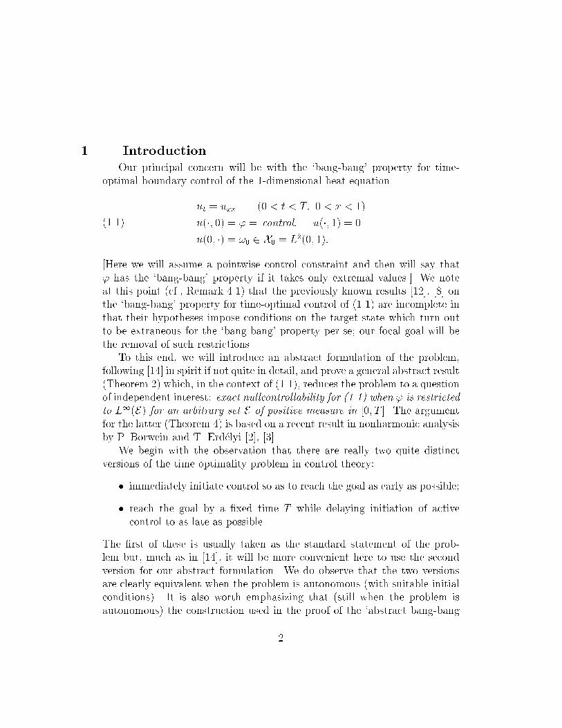
1. IntroductionOur principal concern will be with the `bang-bang' property for time-optimal boundary control of the 1-dimensional heat equationut = uxx (0 < t < T; 0 < x < 1)u(�; 0) = ' = control; u(�; 1) = 0u(0; �) = !0 2 X0 = L2(0; 1):(1.1)[Here we will assume a pointwise control constraint and then will say that' has the `bang-bang' property if it takes only extremal values.] We noteat this point (cf., Remark 4.1) that the previously known results [12], [8] onthe `bang-bang' property for time-optimal control of (1.1) are incomplete inthat their hypotheses impose conditions on the target state which turn outto be extraneous for the `bang-bang' property per se; our focal goal will bethe removal of such restrictions.To this end, we will introduce an abstract formulation of the problem,following [14] in spirit if not quite in detail, and prove a general abstract result(Theorem 2) which, in the context of (1.1), reduces the problem to a questionof independent interest: exact nullcontrollability for (1.1) when ' is restrictedto L1(E) for an arbitrary set E of positive measure in [0; T ]. The argumentfor the latter (Theorem 4) is based on a recent result in nonharmonic analysisby P. Borwein and T. Erd�elyi [2], [3].We begin with the observation that there are really two quite distinctversions of the time-optimality problem in control theory:� immediately initiate control so as to reach the goal as early as possible;� reach the goal by a �xed time T while delaying initiation of activecontrol to as late as possible.The �rst of these is usually taken as the standard statement of the prob-lem but, much as in [14], it will be more convenient here to use the secondversion for our abstract formulation. We do observe that the two versionsare clearly equivalent when the problem is autonomous (with suitable initialconditions). It is also worth emphasizing that (still when the problem isautonomous) the construction used in the proof of the `abstract bang-bang2

principle', Theorem 2, below, could equally well be used directly for a proofof the `bang-bang' property in the context of `version 1', with no restrictionon the initial data.In the context of `version 2', we adjoin to (1.1) the target condition thatthe pro�le at time T belong to a prescribed setu(T; �) 2 ST(1.2)and formulate the time-optimality problem as �nding a pair ('; �) whichmaximizes � subject to the admissibility constraints that, for a given set-valued function A : [0; T ]! 2IR, one has(i) '(t) = '�(t) = given for 0 � t < �(ii) '(t) 2 A(t) for � � t � T(iii) the solution u of (1.1) using this control 'satis�es (1.2).(1.3)We interpret '� as a `trivial' or `passive' control (e.g., '� � 0) so � representsthe time at which we initiate `active' control and maximizing � is just min-imizing the duration (T � �) of the actively controlled interval. [If !0 = 0,'� � 0, then (1.1) gives u(�; �) = 0 so, if also A(t) were independent of t, wecould translate [�; T ] to [0; T �� ] to get the usual `earliest arrival' (version 1)for this autonomous problem.] Concerning the set function A(�), we assumethat a(t); b(t) 2 A(t) and a(�); b(�) 2 L1(0; T )for a(t) := minfA(t)g; b(t) := maxfA(t)g:(1.4)We emphasize that to obtain the `bang-bang' property we need imposeno hypotheses whatsoever on the data f!0; T; ST ; '�g beyond the implicitassumption that such a time-optimal control does exist. We do note thatthe usual argument gives existence of an optimizer in the setting above withST = f!Tg, provided only that the data are compatible (i.e., there is somecontrol satisfying (1.3)) | and this `reachability' is the only restriction to beimposed regarding the target state !T in XT = L2(0; 1).For (1.1), (1.3) with ST = f!Tg, (1.4), we will show thatpointwise ae on [�; T ], the values of any time-optimal control 'must be either '(t) = a(t) or '(t) = b(t), with a; b as in (1.4-ii),3

and that this time-optimal control ' is unique. Note that in this situationthe control ' is a scalar function of t and this strongly a�ects the ease withwhich we can use Theorems 1, 2 to obtain such a `bang-bang' property. Wewill, however, comment in Section 4 on the related situation in which onehas control at both ends of the interval sou���x=0 = '1; u���x=1 = '2(1.5)and the control ' := ('1; '2) is then an IR2-valued function on [0; T ].2. Evolutionary abstract control systemsWe begin by recalling from [14], in slightly modi�ed form, the notion ofan evolutionary abstract control system. Consider I0 := [0; T ] as an ordercategory, i.e., writing I = I 0I 00 for I = [r; t] means I 00 = [r; s]; I 0 = [s; t]with 0 � r � s � t � T ; let (X ;E) be a functor from I0 to the category ofBanach spaces and continuous linear maps so I = [r; t] gives EI : Xr ! Xtwith I = I 0I 00 implying EI = EI0 �EI00 |i.e.,Er;t = Es;tEr;s : Xr ! Xs ! Xt for r � s � t:(2.1)In general, E�� represents uncontrolled system evolution for a possibly non-autonomous well-posed problem. Next we asociate control spaces UI = Ur;tto the intervals I = [r; t] � I0. We always think of each UI as a space offunctions de�ned on I | e.g., UI = L2(I) | so when I = I 0I 00 we maydecompose ' 2 UI into a pair of functions ('0; '00), de�ned on I 0 and I 00,respectively, by restriction maps 0; 00. We then ask that '0 = 0' 2 UI0and '00 = 00' 2 UI00 . The control maps Cr;t : Ur;t ! Xt must satisfy theobvious identity Cr;t = Cs;t0s +Es;tCr;s00s(2.2)for any such decomposition (any choice of s 2 [r; t]).Given any Banach space V with an injection IV : V ! UI | so we maythink of V as consisting of functions with support in (some speci�ed subsetof) I = [t; T ] | we say that V has the nullcontrollability property and writeV 2 NCt;T if there is a nullcontrol v 2 V for each `initial state' in Xt, i.e., ifFor each x = xt 2 Xt there is some v 2 V such thatEt;Tx +CVv = 0 (CV := Ct;T IV) :(2.3) 4

[Clearly, if V 2 NCt;T for some V ,! UI , then UI 2 NCt;T . We recallTheorem 1 of [14]: If Ut;T 2 NCt;T , then Ks = K0t for all s � t, whereKs := R(Es;T ) +R(Cs;T ) and K0s := R(Cs;T ).] Slightly more delicate than(2.3), but useful later, is the restricted nullcontrollability property : we writeV 2 NC rt;T ifFor each x 2 R(C0;t) � Xt there is some v 2 V such thatEt;Tx+CVv = 0:(2.4)We will need the following result, which we present in full although theargument is already known in somewhat di�erent contexts.THEOREM 1: If V 2 NCt;T , (respectively, V 2 NC rt;T ) then there is aconstant KV such that v in (2.3) (respectively, in (2.4)) may be chosen withkvkV � KkxkXt for any K > KV ; dually, if V 2 NCt;T one haskE�t;T �kX �t � KVkC�V �k(2.5)for � 2 X �T with the V�-norm on the right. Conversely, if V contains a dualspace (W� � V) and C�V � 2 W for a dense set D of � 2 X �T , then (2.5) |using the W-norm on the right for � 2 D | implies that V 2 NCt;T .Proof: For brevity we now write simply E for Et;T and C for CV :=Ct;T IV . Clearly, V 2 NCt;T is equivalent to range containment:R(E) � R(C) =: K0(V) � XT :Set V := V=N (C) with an injective induced map C : V ! XT (i.e., Cv =CV v for v 2 v 2 V) and let� := f(x; v) : Ex+ Cv = 0g � Xt � V:Note that � is a subspace and is the graph of a linear map L = LV : Xt ! Vwhich is well-de�ned on all of Xt by (2.3) and the injectivity of C. Since � isclosed (as E; C are continuous), it follows that LV is bounded, by the ClosedGraph Theorem, and the bound on kvk with KV = kLk follows from thede�nition of the quotient space norm on V . Simply replacing Xt by R(C0;t)in the argument above now gives the bound when V 2 NC rt;T . To obtain (2.5)when V 2 NCt;T , we note that the construction of L givesE = �CL so, dually, E� = �L�C�5

with L� : V� ! Xt�. We then have kL�k = kLk =: KV and, since hC��; vi =hC��; vi for v 2 v 2 V and � 2 XT �, this gives (2.5).For the converse, consider any � 2 C�D | i.e., � = C� � for some � 2D � X �T | we can set � := �E��, noting that if � is non-unique (so also� = C�0 with �0 2 D) then (2.5) ensures that kE�(� � �0)k = 0 so � iswell-de�ned. Now, arbitrarily �xing x = xt 2 Xt , we consider� : � 7�! hx; �i = �hx;E��ifor such �. It is clear that the functional � is linear on C�D � W and thatjh�; �ij = jhx; �ij � kxkk�k � kxkKk�k:Thus, � extends by continuity to theW-closure C�D and then, by the Hahn-Banach Theorem, to a linear functional v on W (i.e., v 2 W� � V) withoutincrease of norm so kvk � KVkxk. SincehCv; �i = hv;C��i = �hx;E��i = h�Ex; �ifor � dense in XT �, it follows that Ex +Cv = 0 and v 2 V is a nullcontrolfor x. As x 2 Xt was arbitrary, we have (2.3) so V 2 NCt;T as asserted.3. Time-optimalityWe now turn to formulation of the abstract time-optimality problem. Itwill be convenient here to abuse notation slightly by thinking of U = U0;Tas the common domain of the control maps Cs;t : U ! Xt , omitting explicitindication of the operators; note that we think of Cs;t' as depending onlyon `the part of ' between s and t' | so N (Cs;t) � N ([s;t]) where, in theobvious notation, [s;t] := 0s;[0;t]00t;[0;T ] = 00t;[s;T ]0s;[0;T ]:Fixing the passive control '� 2 U , a basic assumption is that for each s 2(0; T ) we have ' 2 U ) Ps' := �'� on [0; s)' on [s; T ] 2 U(3.1) 6

or, more formally, 0sPs' = 0s' and 00sPs' = 00s'� ; note that Ps will notgenerally be linear unless '� � 0. We impose the continuity condition thatCr;tPs'! Cr;t' as s& r:(3.2)for 0 � r < t � T | which just says that changing ' on the vanishinglysmall interval [r; s] has vanishingly small control e�ect at any t > r.The data for the time-optimality problem will bex0 2 X0; '� 2 U ; A � U ; ST � XT(3.3)where x0 is an initial state, '� the `passive control', A is a constraint set, andST the target set. We will require | to simplify our statement, rather thanas a restriction on A | that ' 2 A implies Ps' 2 A for each s. The set ofadmissible pairs P = P(A;ST ; x0; '�) is then de�ned asP := f('; �) 2 A� [0; T ] : ' = P�'; [E0;Tx0 +C0;T'] 2 STg(3.4)and we say that a control �' or, more precisely, an admissible pair ( �'; �� ) 2 Pis time-optimal (with respect to this data) if it maximizes � over ('; �) 2 P.We will say that ' 2 U is `slack with respect to (A;V)' (for a Banachspace V with IV : V ! U) if there is some " > 0 such that['+ IVv] 2 A for all v 2 V with kvkV < ":(3.5)At this point we may state and prove our `abstract bang-bang principle'THEOREM 2: Suppose ' 2 U is slack with respect to (A;V) forsome V 2 NC rt;T . Then ('; �) with � < t cannot be time-optimal with respectto any data set (A;ST ; x0; '�) involving this A.Proof: Note that, while we have written simply IV : V ! U , the condi-tion that V 2 NC rt;T includes the implication that R(IV) is actually in Ut;T sofor s � t one hasPs's = 's for 's := Ps('+ IVv) (any v 2 V):(3.6)Now let Kr be as KV in Theorem 1 applied to this V 2 NC rt;T and let " > 0be as in (3.5). In view of (3.2) with r = � < t, we may choose s =: � closeenough to � (with � < � < t) that~x := C�;t [P�' � '] gives k~xk < "=Kr;(3.7) 7

noting that ~x 2 R(C0;t) � Xt. By Theorem 1 we may then choose v 2 Vsuch that Et;T ~x +Ct;Tv = 0 and kvkV < ":(3.8)Now set ' := P� ('+ IVv) | i.e., ' = 8><>:'� on [0; �)P�' on [�; t)'+ IVv on [t; T ].(3.9)Since kvkV < ", we have [' + IVv] 2 A by (3.5) so also ' 2 A; we haveP� ' = ' by (3.6). Using (2.2) twice, splitting [0; T ] at � and at t, we haveC0;T' = E�;TC0;�'� +C�;T'as ' = '� on [0; �)= E�;TC0;�'� +Et;TC�;t'+Ct;T'(3.10)and, similarly, we haveC0;T ' = E�;TC0;�'� +Et;TC�;tP�'+Ct;T ['+ IVv](3.11)using (3.9). Comparing (3.11) to (3.10) gives (with CV := Ct;T IV as before)C0;T '�C0;T' = Et;TC�;t [P�'� '] +CVv= Et;T ~x +CVv = 0(3.12)by (3.7) and (3.8).It follows that ('; �) 2 P = P(A;ST ; x0; '�) for any data which gives('; �) 2 P: if E0;Tx0 + C0;T' =: xT 2 ST , then also E0;Tx0 + C0;T ' = xTfor the very same xT 2 ST . Since � > � , it would then be impossible for �to be maximal and ' could not be a time-optimal control.To see why we refer to Theorem 2 as an `abstract bang-bang principle', wenote our motivating consequence. Observe, �rst, that in considering scalarcontrols with a uniform pointwise bound as in (1.4), there is some arbi-trariness about the speci�cation of the control space U . We will, somewhatarbitrarily, take U := Lp(0; T ) for some �nite p > 1 (so, in particular, U isre exive) and assume that each of the operators Es;t; Cs;t is continuous forthis choice of U . 8

THEOREM 3: Consider a time-optimality problem, as above, withST closed and convex in XT , scalar control (say, U = Lp(0; T ) for some p � 1),and A of the form:A := f' 2 U : '(t) 2 A(t) ae on [0; T ]g(3.13)with A(�) as in (1.4) and '� 2 A. AssumeFor each t 2 (0; T ), each set E � (t; T ) of positive measure,one has L1(E) 2 NC rt;T :(3.14)Then there is a unique time-optimal control �' and this necessarily has the`bang-bang' property:['(t) = a(t) or '(t) = b(t)] ae on [�; T ](3.15)with a; b as in (1.4).The key to this is that for (3.15) to fail one must havea(t) + " � '(t) � b(t)� " for t 2 E(3.16)for some " > 0 and some set E of positive measure in [�; T ] | perhapsrestricting to an intersection, we may assume E is actually contained in some[�t; T ] with �t > � . We do note that the very existence of a time-optimal controlis not immediately clear at this point since we have not even assumed thatA(t) should be a closed set.Proof: We �rst consider the situation with A replaced by A� whereA� := f' 2 U : '(t) 2 [a(t); b(t)] =: A�(t) ae on [0; T ]g:AsA� is bounded, closed, and convex (hence weakly compact in U = Lp(0; T ) ),the usual argument gives existence of a time-optimal control: Let ('�) bean optimizing sequence so we may assume '� * �' with �� % � ; notingthat C0;T'� * C0;T �', we must have E0;Tx0 +C0;T �' 2 ST whence ( �'; �) isadmissible and so time-optimal.] By (3.14) and Theorem 2, we see that �'cannot be slack with respect to (A�;V) for any V = L1(E) with E of positivemeasure in (�t; T ), �t > � . On the other hand, we have already noted that afailure of (3.15) would give (3.16), which would imply such slackness and give9

a contradiction. Hence, �' must satisfy (3.15) so, by (1.4), we have �' 2 Aand this pair ( �'; �) is also admissible for the original problem. Since theproblem using A� is a relaxed version of that, ( �'; �) must be time-optimalfor the original problem.To see uniqueness, note that if ('; �) were a di�erent time-optimal pairfor the original problem (necessarily with the same �), then we may set~' := ( �' + ')=2 and note that ( ~'; �) is an admissible pair for the problemusing A�, since the system is linear and A�;ST are convex. Whether or not' satis�es (3.15), it is clear that (3.15) cannot hold for ~' on the (assumednonnull) set where ' 6= �'. As above, we then see that ( ~'; �) cannot be time-optimal for that problem, contradicting the assumed maximality of � . Thus,�' is the unique optimal control for the original problem.For the �nite dimensional case (state space IRn) we see that the hypothe-ses above are easily established for control systems governed by_x = Ax+ 'b x(0) = x0:(3.17)COROLLARY 4: The results of Theorem 3 apply to time-optimalityproblems of the indicated form for (3.17), provided A(�) ;b(�) are real-analyticon [0; T ] when this is non-autonomous.Proof: We need only verify the hypothesis (3.14) and for this it is con-venient to take Xt := R(C0;t) for t 2 [0; T ] so, in particular, C = C0;T issurjective to XT . The choice of control space U is not very signi�cant andwe take, e.g., U := L2(0; T ). One easily veri�es that the adjoint map C� isgiven, for � 2 X �T (� IRn), by C� : � 7! hb; yi 2 L2(0; T ) where� _y = A�y; y(T ) = �:(3.18)The range R(C�) = fhb; yig is then �nite dimensional | indeed, as Cis surjective, it follows that C� is injective and dimR(C�) = dimX �T =dimXT � n. The analyticity assumptions on A(�); b(�) ensure that y andhb; yi are real-analytic on [0; T ]. Hence, if hb; yi = 0 on any set E ofpositive measure, one must have hb; yi � 0 on [0; T ]. Thus, the mapLE : � 7! hb; yi���E : X �T ! R(C) ! W (where W consists of the restric-tions to E of functions in R(C�)) is injective and so invertible. Since W10

is �nite dimensional, [LE ]�1 is continuous with W normed as a subspace ofW := L1(E) (so V := L1(0; T ) is just W�) and (2.5) holds, giving (3.14) byTheorem 1. The conclusion is now immediate from Theorem 3.This argument seems new, even for the �nite dimensional case; we do notethat it does not seem to be usefully related to the usual characterization oftime-optimal controls as in the Pontrjagin Maximum Principle.

11

4. Boundary control of the heat equationIn this section we return to consideration of (1.1) as an example of theabstract formulation of Sections 2, 3. Our principal new result is exactboundary nullcontrollability from measurable sets | more precisely, thatL1(E) 2 NCt;T for any set E of positive measure in [t; T ]. This is just (3.14)| one notes that NCt;T and NC rt;T are equivalent here | so Theorem 3 thengives the desired `bang-bang' property for time-optimal boundary control of(1.1).We will take Xt = X := L2(0; 1) for each t 2 [0; T ] and will, e.g., takeU = L2(0; T ), so UI = L2(I) with the obvious interpretations of the oper-ators by restriction. For this autonomous situation one has Er;t = S(t � r)where S(�) is the semigroup on L2(0; 1) corresponding to (1.1) with homo-geneous boundary conditions. Then Cs;t is the control e�ect (so Cs;t : ' 7!u(t; �) where u satis�es (1.1-i; ii) with u(s; �) = 0) and it is standard (cf.,e.g., [10]) that each Cs;t is continuous | indeed, compact | from L2(s; t)to X = L2(0; 1). [We note in passing that there is a well-known explicitrepresentation for this control mapping associated with (1.1) | using convo-lution with a fundamental solution, expressible in terms of a theta function;cf., e.g., [5] p. 171.] The identities (2.1), (2.2) are clear in this context. Forthis U there is no di�culty in de�ning Ps and the continuity condition (3.2)here follows a fortiori from the stronger fact that Ps ! Pr (strongly onU = L2(0; T )) as s! r.To compute the adjoint maps E��t;T ; C��t;T we consider u satisfying (1.1) for�t < t � T with u(�t; �) � 0 and y satisfying�yt = yxx (0 < t < T; 0 < x < 1)y(T; �) = � 2 X �T = L2(0; 1)y(�; 0) � 0 � y(�; 1):(4.1)A simple computation involving (1.1) with u(�t; �) = 0, (4.1), and an integra-tion by parts gives the identityZ 10 uy dx����t=T = Z T�t ' [yx(�; 0)] dt12

and, since u(T; �) = C�t;T' here, this givesC��t;T : X �T ! L2(�t; T ) � L2(0; T ): � 7�! := yx(�; 0)���[�t;T ]:(4.2)Even more simply, (4.1) givesE��t;T : X �T ! X ��t = L2(0; 1) : � 7�! y(�t; �):(4.3)It will be necessary to represent y in terms of the eigenfunctions and eigen-values �k(x) := p2 sinq�kx; �k := k2�2(4.4)so that � =Xk ck�k gives 8>>><>>>: y =Xk cke��k(T�t)�k =Xk �q2�k ck� e��k(T�t):(4.5)Our immediate observation is that� 2 D := span f�kg ) C��t;T� = 2 M =M(�) := span fe��k(T�t)gwhere � := f�k : k = 1; 2; : : :g with, looking to a somewhat more generalsetting, 0 < �1 < �2 < : : : such that �k1=�k is convergent | as is obviouslythe case here.Our starting point will be an inequalityky(0; �)kL2(0;1) �M�tkyx(�; 0)kL2(0;�t)(4.6)for solutions of (4.1); it is su�cient to consider this only for � 2 D. Werecognize this as (2.5) | giving (2.3) by Theorem 1 | corresponding tohaving U0;�t 2 NC0;�t , replacing T by �t here. We will take this nullcontrolla-bility as `well-known' | but note that essentially this inequality (with timereversed and an interchange of Dirichlet and Neumann conditions) was theprincipal result of [11], with the nullcontrollability form given in [4]). From(4.6) with time reversed, one sees clearly the interpretation of (2.5) as assert-ing well-posed observability : predicting the terminal state from (boundary)observations without knowing the initial state.13

Our major new resource is an inequality recently obtained by P. Borweinand T. Erd�elyi; this is Theorem 5.6 of [2], but see also [1], [3].THEOREM (BE): Assume �k1=�k <1, etc. Then, for every q > 0,s > 0, � 2 (0; 1), there is a constant c = cq(s; �;�) such that:For every set A � [�; 1] with meas A � s one haskpkL1(0;�) � ckpkLq(A)(4.7)for every `polynomial' p 2 M0 =M0(�) := n�kakx�ko.For our present purposes, we make the substitution x = e�(T�t) and set� = e�(T��t) so t 2 [0; �t]; [�t; T ]; E correspond, respectively, to x 2 [e�T ; �] �[0; �]; [�; 1]; A and M corresponds to M0; noting that meas A � �meas Efor E � [�t; T ], one easily sees that, specializing to q = 1, (4.7) gives just theinequality we will need:k ~ kL2(0;�t) � ~ck ~ kL1(E) for ~ 2 M(4.8)with ~c = p�t c1(�meas E ; �;�) for any set E of positive measure in [�t; T ].At this point we are in a position to state and prove our second princi-pal result, on exact boundary nullcontrollability of the one-dimensional heatequation from arbitrary sets of positive measure.THEOREM 4: Let T > 0 and suppose E � [0; T ] has positivemeasure. Then there is a constant K such that:For every !0 2 X = L2(0; 1) there is a control ' such thatj'(t)j � Kk!0kX for t 2 E , '(t) = 0 for t =2 E ,and the solution u of (1.1), using ', has u(T; �) = 0.Proof: This follows directly from the results we have already developed.Choose any �t > 0 such that E \ [�t; T ] has positive measure; set W := L1(E)and V := W� = L1(E). Consider y(0; �) = E�0;T� and ~ = = C�0;T� for� 2 D. Then (4.6) and (4.8) with E replaced by E give ky(0; �)kL2(0;1) �M�t~ck kL1(E) or, equivalently,kE�0;T�kX � � KVkC�V�kWwhich we recognize as (2.5). The second part of Theorem 1 then givesV 2 NC�t;T which, since E � E so V ,! L1(E), gives precisely the con-clusion of the present theorem. 14

COROLLARY 6: The results of Theorem 3 apply to the time-optimality problem for (1.1).Proof: Theorem 5 just gives the hypothesis (3.14) in this context soTheorem 3 applies.The argument in Theorem 5 establishing that for each E in [t; T ] of pos-itive measure one has L1(E) in NC r and hence that Theorem 3 applies,shows (cf. Theorem V 1.1 of [7]) that the vector measurem : B[0; T ]! XT = L2(0; 1) : E 7! C0;T (�E)is a Liapunov measure | i.e., for each Borel set F � [0; T ] of positivemeasure, the set fm(E) : E � Fg is a convex, weakly compact subset ofL2. The control-theoretic implications of this property of m are discussed inChapters V and IX of [7].REMARK 4.1: We remark that the `bang-bang' property for time-optimal controls is classical for the �nite-dimensional case, but has previouslybeen shown in the context of boundary controls of the heat equation onlywith the imposition of a `slackness condition' on the target state: the controlconstraint has the form j'j � M where it is to be known that the targetis actually reachable (in some time) subject to j'j � M 0 with the slacknessconsisting of asking that M > M 0. Some years ago, when [12] appeared, wefelt that this condition might be an artifact of the proof technique and weattempted to demonstrate the `bang-bang' property without it, i.e., for arbi-trary (reachable) targets. We failed at that time: the gap in our argumentwas the need for an estimate such as (4.7) and it is the recent availabilityof the result by P. Borwein and T. Erd�elyi [1] which has enabled us now toreturn successfully to the problem.It should be noted that a newer proof of the `bang-bang' property waspresented in W. Krabs' book [8], but this proof also imposes an auxiliarycondition on the target state !T . The result, Theorem 2.4.13 of [8], is for-mulated in terms of a moment problem, so some translation is necessary forcomparison. He requires that c 2 W where c = (ck) is the sequence of Fourier15

coe�cients of the target u� and the space W is such that this requirementis equivalent to asking that u� is a limit | in the sense that di�erences arereachable by controls with L1-norm approaching 0 | of targets of the spe-cial form ~u("; �) for " > 0 and ~u satisfying the equation ~ut = ~uxx with controlvanishing on [T � "; T ]. Certainly the special targets then have ~u("; x) = 0at x = 0; 1 so this, in particular, will also be true in the limit, i.e., for thetargets to which Krabs' Theorem 2.4.13 would apply. Krabs also providesTheorem 2.4.14, explicitly following ideas of [12], giving the conclusion withessentially the same `slackness condition' mentioned earlier; this conditioncertainly implies that j~u(0)j � M 0 < M . Thus, neither of these theoremswould apply to use as target, e.g., the trivially reachable state obtained bytaking ' �M on [0; T�]. In comparison, we emphasize that we have imposedno requirement on the target to get the `bang-bang' property for a time-optimal control except as is implicit in the very existence of such a control.The paper [12] considers the n-dimensional case (a bounded spatialregion � IRn with control ' on [0; T ]� @) subject to a constraint of theform j'(t; x)j �M ae for 0 � t � T; x 2 @:(4.9)To use our present approach to prove the strong form of the `bang-bang' prop-erty | that j'�j =M ae on [0; T �]� @ | would require an n-dimensionalform of Theorem 4, showing exact nullcontrollability with controls in L1(E)where E is now an arbitrary subset of positive measure in [0; T �]� @. Thisseems well out of reach by currently available ideas | indeed, even the null-controllability from a patch (E = [0; T �] � P with P � @ open but small)has only recently been demonstrated ([9], compare [13]). On the other hand,it seems to be a tractable open problem to show the weaker `bang-bang'property that k'�(t; �)kL1(@) =M ae on [0; T �] by showing nullcontrollabil-ity from L1(E � @) with E of positive measure in [0; T �] as earlier.Note that each of the results above obtains the `bang-bang' propertyby way of the adjoint characterization: ' = fM where vx � M ;�M wherevx � �Mg for some solution v of the adjoint problem. A plausible conjec-ture is that the additional restriction on the target state might be signi�cantto ensure this characterization (so there might conceivably be examples forwhich this characterization fails in the absence of some such slackness condi-tion; this could be a subject for future investigation), although we have seenthat it is not necessary for the `bang-bang' property itself.16

REMARK 4.2: An essentially identical argument works if we replacethe heat equation in (1.1) by ut = (pux)x � qu(4.10)and/or replace the Dirichlet boundary conditions there by some alternativetype of boundary control. For this case we let f�k; zkg be the eigenvalues andeigenfunctions of the Sturm-Liouville operator A : z 7! �(pz0)0 + qz whose(homogeneous) boundary conditions are those of the new form of boundarycontrol.Similarly, one could consider the problem with scalar control in theequation itself: ut = (pux)x � qu+ '(t)b(4.11)for some speci�ed b(�) 2 X , using homogeneous boundary condition. Inthis connection one might note Henry's example [6] of a problem with time-optimal control not of bang{bang form | as in (4.10) but e�ectively con-sidering version 1 of the time-optimality problem with time-dependent con-straints, so it does not correspond to the situation we have analyzed.REMARK 4.3: We may consider the problem with a non-scalar con-trol: ''' = ['0; '1] so the boundary conditions in (1.1) are replaced byu(�; 0) = '1 u(�; 1) = '2(4.12)and in (1.3) we take A(t) = K � IR2 where K is a closed, bounded, convexset. Here we may distinguish two forms of the `bang-bang' property:weak: ae on [0; T �] one has '''(t) 2 @Kstrong: ae on [0; T �] one has '''(t) an extreme point of K.The weak form is immediate from the previous arguments: if there wereE � [0; T ] with positive measure for which ''' remained in the interior, thenwe could obtain a contradiction as in the proof of Theorem 2, perturbing onlythe component '0 as there. For the strong form one needs a modi�cationof this to avoid the possibility that ''' might remain interior to some facewithin @K so that one must consider perturbations with a linear restriction:17

~'(t) = '(t)c for some nonzero c 2 IR2. What would be needed then isthe appropriate modi�cation of the inequality (4.6), obtainable along similarlines. To illustrate the situation, consider �rst K = [0; 1] � [0; 1] Any casewhere ''' is weakly optimal but not strongly optimal can be reduced to thefollowing: for a set E of positive measure in [�; T ] and some " > 0, one has'1(t) 2 ("; 1 � ") with '2(t) 2 f0; 1g for all t 2 E . By selecting � > � butclose, we can ensure that E 0 = E \ [�; T ] has positive measure and that thestate ! 0� produced at � by use of the modi�ed controls '0i(t) = f'i(t) fort < � ; = 0 for t 2 [�; � ] di�ers from the state !� produced by the original''' = ('1; '2) by less than "=Kr, i.e., k! 0� � !�k < "=Kr. Consequently, bymodifying '01 by v supported on E 0 and of supnorm< ", we obtain | as inthe proof of Theorem 2 | that ('01 + v; '02) attains the same target !T as''' yet with � replaced by the larger � , contradicting the assumed optimalityof � . On the other hand, if we take K = f(x; y) : x; y � 0; x + y � 1g, itis clear that such an argument is only available if one knows that pairs with'1 + '2 = 0 on E are available as nullcontrols for the state perturbation.Such `odd' control pairs only produce corresponding odd states and so canonly compensate for odd state perturbations. Hence our argument cannot beexpected to work in this setting, although we cannot on this basis concludethat the `bang-bang' property fails.Similar considerations apply if one would generalize (4.11) tout = (pux)x � qu+ �j'j(t)bj(4.13)with pointwise constraints imposed on the vector control ''' = ['1; : : : ; 'J ].REMARK 4.4: There is little di�culty in generalizing the abstractTheorem 3 to treat state-dependent constraints. It is convenient to takea space XX = fx(�)g of `controlled trajectories', where the state trajectoryis de�ned by x(t) := C0;t' for t 2 [0; T ]; ' 2 U ; we assume the topologyimposed on XX is such that the linear map X : ' 7! x(�) : U ! XX iscontinuous. By a `state-dependent constraint' we mean a set-valued function(t; x) 7�! A(t; x) � IR for t 2 [0; T ]; x 2 XX(4.14)so the control restriction (1.3-ii) becomes' 2 A := f' 2 U : '(t) 2 A(t;X') ae on [0; T ]g:(4.15) 18

We continue to take U = Lp(0; T ) and to assume (1.4), now also writinga(t) = a(t; x); b(t) = b(t; x); we will further assume that one has uniformbounds: a � a(t; x) � b(t; x) � b for all x 2 XX . Finally, we need a mildcontinuity condition4'n * �'(weak convergence in U) with (4.15) for each nimplies: a(t;X �') � �'(t) � b(t;X �') ae on [0; T ]:(4.16)We may then argue much as in the proof of Theorem 3. If 'n is an optimizingsequence for the time-optimality problem given by (4.15), we have 'n * �'| using our assumptions on A(��) and extracting a subsequence if necessary| so we may set A�(t) := [a(t;X �'); b(t;X �')] and have �'(t) 2 A�(t) ae on[0; T ]. As in the proof of Theorem 3, we consider the time-optimality problemusing A� for A to obtain a (unique) time-optimal control '. As there, ' hasthe `bang-bang' property and so is also admissible for the original problem| whence the control times � are the same and we can conclude that ' = �'so that this is the unique time-optimal control for the original problem.Acknowledgements: Mizel wishes to acknowledge partial support of thisresearch by the US National Science Foundation under grants DMS 9201221,DMS 9500915. He also wishes to express his appreciation to Peter Borweinfor informing him of the recent results achieved by Borwein and Erd�elyi in[1] and to Greg Knowles for very stimulating discussions on this topic severalyears ago.References[1] P. Borwein and T. Erd�elyi, M�untz spaces and Remez inequalities,Bull. AMS 32, pp. 38{42 (1994).4For example, it is not hard to see that (4.16) will hold if one can take XX compact inC([0; T ]! X ) and if, with A(t) = A(t; x(t)) so A : [0; T ]�X ! 2IR, one hasrn ! �r; zn ! �z; rn 2 A(t; zn) ) a(t; �z) � �r � b(t; �z):19

[2] P. Borwein and T. Erd�elyi, Generalizations of M�untz's Theorem via aRemez-type inequality for M�untz spaces, preprint (Simon Fraser Univ.)1994.[3] P. Borwein and T. Erd�elyi, Polynomials and Polynomial Inequalities,Springer-Verlag, New York, 1995.[4] H.O. Fattorini and D.L. Russell, Exact controllability theorems for linearparabolic equations in one space dimension, Arch. Rat. Mech. Anal. 43,pp. 271{292 (1971).[5] G. Hellwig, Partial Di�erential Equations, Blaisdell, New York, 1964.[6] J. Henry, Un contre-exemple en th�eorie de la commande en temps min-imal des syst�emes paraboliques, C.R. Acad. Sci. Paris (s�erie A) 289,pp. 87{89 (1979).[7] I. Kluvanek and G. Knowles, Vector Measures and Control Systems,(Mathematics Studies #20), North-Holland, 1975.[8] W. Krabs, On Moment Theory and Controllability of One-DimensionalVibrating Systems and Heating Processes (Lecture Notes in Control andInf. Sci. #173), Springer-Verlag, New York, 1992.[9] G. Lebeau and L. Robbiano, Controle exact de l'�equation de la chaleur,Comm. P.D.E, 20, pp. 335-356, (1995).[10] J.L. Lions and E. Magenes, Non-Homogeneous Boundary Value Prob-lems and Applications, vol. II, Springer-Verlag, Berlin, 1972.[11] V.J. Mizel and T.I. Seidman, Observation and prediction for the heatequation, I, J. Math. Anal. Appl. 28, pp. 303{312 (1969).[12] E.J.P.G. Schmidt, The `bang-bang' principle for the time-optimal prob-lem in boundary control of the heat equation, SIAM J. Control Optim.18, pp. 101{107 (1980).[13] T.I. Seidman, Observation and prediction for the heat equation, IV:patch observability and controllability, SIAM J. Control Optim. 15,pp. 412{427 (1977). 20

[14] T.I. Seidman, Time-invariance of the reachable set for linear controlproblems, J. Math. Anal. Appl. 72, pp. 17{20 (1979)

21