AMVs at the Met Office: activities to improve their impact in NWP
33
© Crown copyright Met Office AMVs at the Met Office: activities to improve their impact in NWP James Cotton, Mary Forsythe, Roger Saunders, Richard Marriott 11 th International Winds Workshop, Auckland, 20-24 February 2012
-
Upload
khangminh22 -
Category
Documents
-
view
3 -
download
0
Transcript of AMVs at the Met Office: activities to improve their impact in NWP

© Crown copyright Met Office
AMVs at the Met Office: activities to improve their impact in NWP James Cotton, Mary Forsythe, Roger Saunders, Richard Marriott
11th International Winds Workshop, Auckland, 20-24 February 2012
© Crown copyright Met Office
Contents
This presentation covers the following areas • Current status
• Temporal Thinning
• Revisit observation errors / spatial blacklisting
© Crown copyright Met Office © Crown copyright Met Office
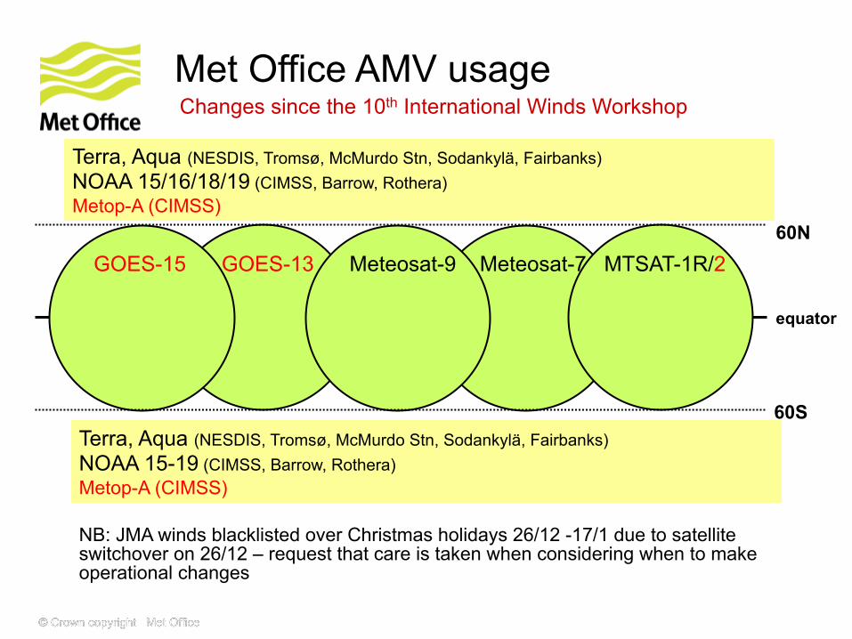
Met Office AMV usage •
equator
60N
60S
GOES-15 GOES-13 Meteosat-9 Meteosat-7 MTSAT-1R/2
Terra, Aqua (NESDIS, Tromsø, McMurdo Stn, Sodankylä, Fairbanks) NOAA 15-19 (CIMSS, Barrow, Rothera) Metop-A (CIMSS)
May 2008
Terra, Aqua (NESDIS, Tromsø, McMurdo Stn, Sodankylä, Fairbanks) NOAA 15/16/18/19 (CIMSS, Barrow, Rothera) Metop-A (CIMSS)
Changes since the 10th International Winds Workshop
NB: JMA winds blacklisted over Christmas holidays 26/12 -17/1 due to satellite switchover on 26/12 – request that care is taken when considering when to make operational changes

© Crown copyright Met Office
Temporal thinning
© Crown copyright Met Office
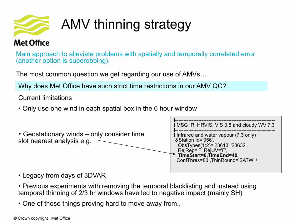
AMV thinning strategy •
The most common question we get regarding our use of AMVs…
Why does Met Office have such strict time restrictions in our AMV QC?..
Current limitations • Only use one wind in each spatial box in the 6 hour window
!------------------------------------------------------------ ! MSG IR, HRVIS, VIS 0.8 and cloudy WV 7.3 !------------------------------------------------------------ ! Infrared and water vapour (7.3 only) &Station Id='056', ObsTypes(1:2)='23613','23632', RejRep='F',RejUV='F', TimeStart=0,TimeEnd=40, ConfThres=80.,ThinRound='SATW' /
• Legacy from days of 3DVAR • Previous experiments with removing the temporal blacklisting and instead using temporal thinning of 2/3 hr windows have led to negative impact (mainly SH) • One of those things proving hard to move away from..
• Geostationary winds – only consider time slot nearest analysis e.g.
Main approach to alleviate problems with spatially and temporally correlated error (another option is superobbing).
© Crown copyright Met Office
© Crown copyright Met Office
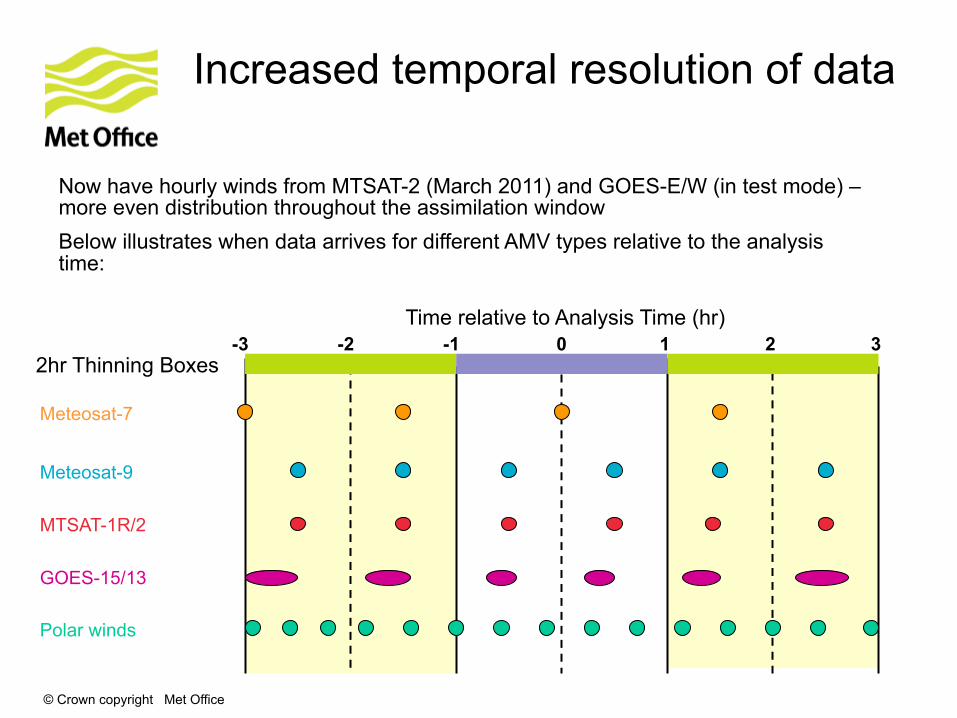
Increased temporal resolution of data
-3 -2 -1 0 1 2 3 2hr Thinning Boxes
Meteosat-7
Time relative to Analysis Time (hr)
Meteosat-9
MTSAT-1R/2
GOES-15/13
Polar winds
Now have hourly winds from MTSAT-2 (March 2011) and GOES-E/W (in test mode) – more even distribution throughout the assimilation window Below illustrates when data arrives for different AMV types relative to the analysis time:
© Crown copyright Met Office
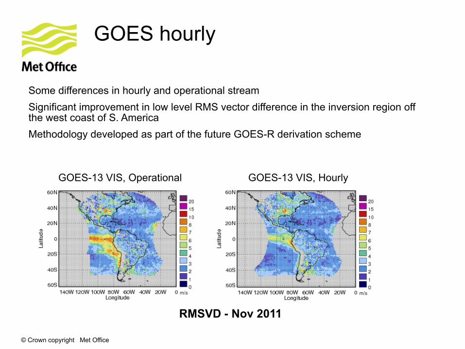
GOES hourly
Some differences in hourly and operational stream Significant improvement in low level RMS vector difference in the inversion region off the west coast of S. America Methodology developed as part of the future GOES-R derivation scheme
GOES-13 VIS, Operational GOES-13 VIS, Hourly
RMSVD - Nov 2011
© Crown copyright Met Office
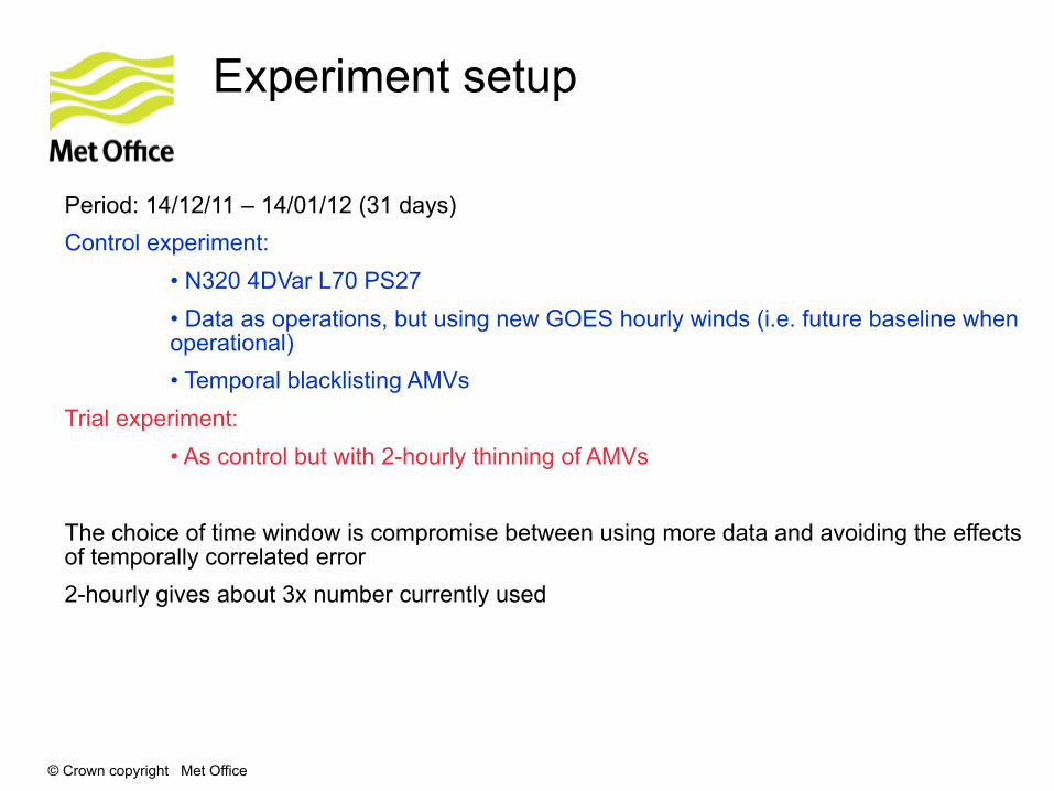
Experiment setup
Period: 14/12/11 – 14/01/12 (31 days) Control experiment:
• N320 4DVar L70 PS27 • Data as operations, but using new GOES hourly winds (i.e. future baseline when operational) • Temporal blacklisting AMVs
Trial experiment: • As control but with 2-hourly thinning of AMVs
The choice of time window is compromise between using more data and avoiding the effects of temporally correlated error 2-hourly gives about 3x number currently used
© Crown copyright Met Office
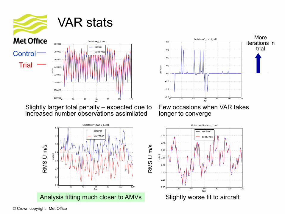
VAR stats
Slightly larger total penalty – expected due to increased number observations assimilated
Control Trial
Few occasions when VAR takes longer to converge
More iterations in
trial
Analysis fitting much closer to AMVs
RM
S U
m/s
RM
S U
m/s
Slightly worse fit to aircraft

© Crown copyright Met Office
Trial results - NWP Index vs Observations vs Analyses
Season 1 +0.5 -1.7
NWP index positive versus observations, but strongly negative versus analysis Biggest problem at T+24 in tropics and SH for wind and temps Especially large hits for W250
Positive impact Positive impact
observations analyses
Weighted basket of skill scores with most weight on T+24 performance
© Crown copyright Met Office
What next
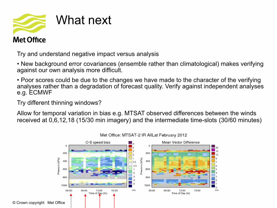
Try and understand negative impact versus analysis • New background error covariances (ensemble rather than climatological) makes verifying against our own analysis more difficult. • Poor scores could be due to the changes we have made to the character of the verifying analyses rather than a degradation of forecast quality. Verify against independent analyses e.g. ECMWF Try different thinning windows?
Allow for temporal variation in bias e.g. MTSAT observed differences between the winds received at 0,6,12,18 (15/30 min imagery) and the intermediate time-slots (30/60 minutes)
© Crown copyright Met Office
Revisit observation errors
© Crown copyright Met Office © Crown copyright Met Office
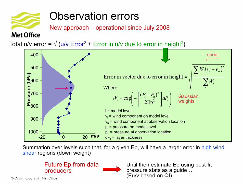
Total u/v error = √ (u/v Error2 + Error in u/v due to error in height2)
Future Ep from data producers
Until then estimate Ep using best-fit pressure stats as a guide… (Eu/v based on QI)
Observation errors New approach – operational since July 2008
i = model level vi = wind component on model level vn = wind component at observation location pi = pressure on model level pn = pressure at observation location dPi = layer thickness
400 500 600 700 800 900
1000 -20 0 20 m/s
Pres
sure
(hPa
) ( )
∑
∑ −=
ii
inii
W
vvW 2
height in error toduein vector Error
⎟⎟⎠
⎞⎜⎜⎝
⎛⎥⎦
⎤⎢⎣
⎡ −−= i
nii dPPPW 2
2
Ep2)(exp
Where
Gaussian weights
shear
Summation over levels such that, for a given Ep, will have a larger error in high wind shear regions (down weight)
© Crown copyright Met Office
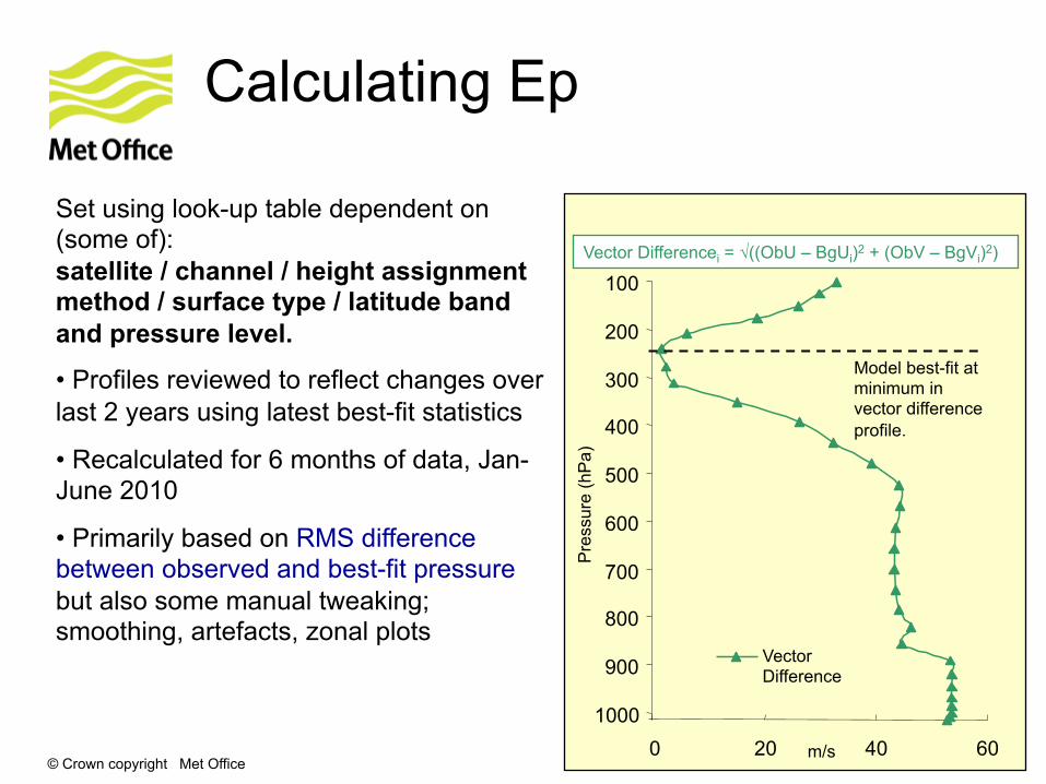
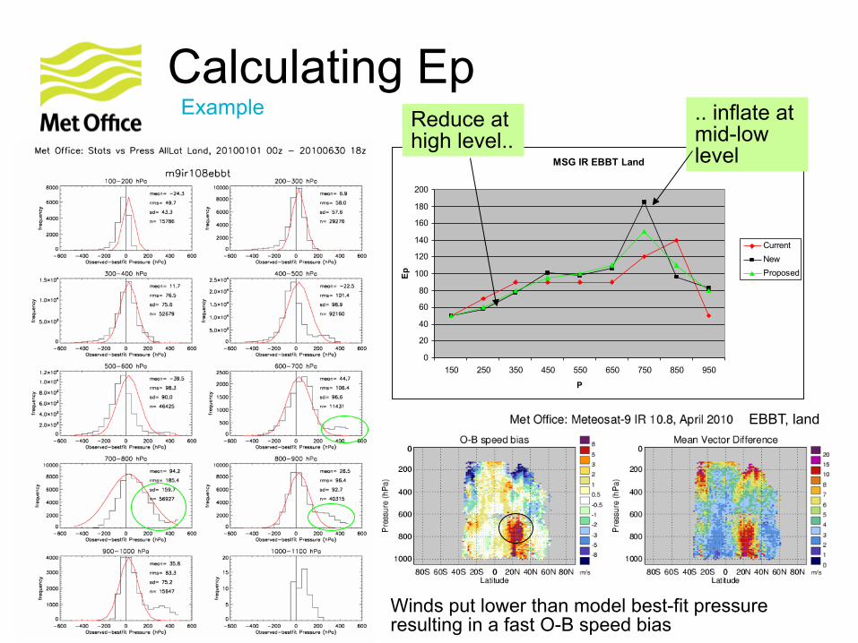
Calculating Ep
Set using look-up table dependent on (some of): satellite / channel / height assignment method / surface type / latitude band and pressure level.
• Profiles reviewed to reflect changes over last 2 years using latest best-fit statistics
• Recalculated for 6 months of data, Jan-June 2010
• Primarily based on RMS difference between observed and best-fit pressure but also some manual tweaking; smoothing, artefacts, zonal plots
Vector Differencei = √((ObU – BgUi)2 + (ObV – BgVi)2)
100 200 300 400 500 600 700 800 900
1000 0 20 40 60 m/s
Pre
ssur
e (h
Pa)
Vector Difference
Model best-fit at minimum in vector difference profile.
© Crown copyright Met Office
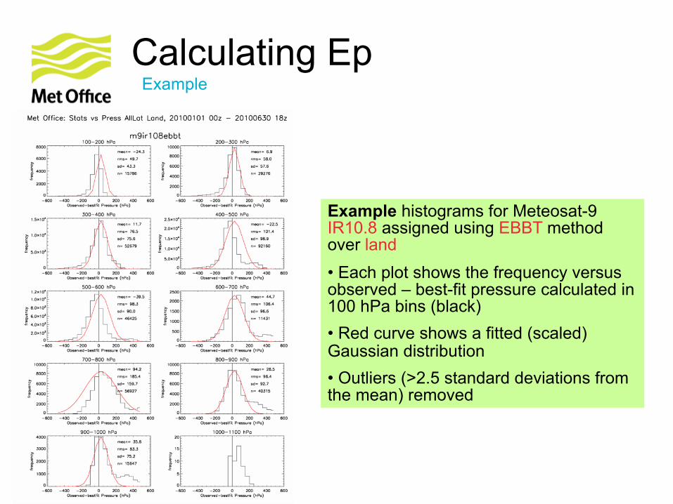
Calculating Ep Example
Example histograms for Meteosat-9 IR10.8 assigned using EBBT method over land • Each plot shows the frequency versus observed – best-fit pressure calculated in 100 hPa bins (black) • Red curve shows a fitted (scaled) Gaussian distribution • Outliers (>2.5 standard deviations from the mean) removed
© Crown copyright Met Office
Calculating Ep Example
MSG IR EBBT Land
0
20
40
60
80
100
120
140
160
180
200
150 250 350 450 550 650 750 850 950
P
Ep
Current NewProposed
.. inflate at mid-low level
Reduce at high level..
Winds put lower than model best-fit pressure resulting in a fast O-B speed bias
EBBT, land
© Crown copyright Met Office
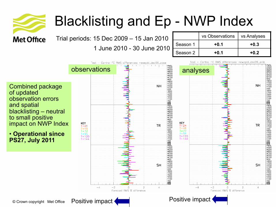
Blacklisting and Ep - NWP Index Trial periods: 15 Dec 2009 – 15 Jan 2010 1 June 2010 - 30 June 2010
vs Observations vs Analyses
Season 1 +0.1 +0.3
Season 2 +0.1 +0.2
Positive impact Positive impact
observations analyses
Combined package of updated observation errors and spatial blacklisting – neutral to small positive impact on NWP Index • Operational since PS27, July 2011

© Crown copyright Met Office
Questions

© Crown copyright Met Office
Updated spatial blacklisting
© Crown copyright Met Office
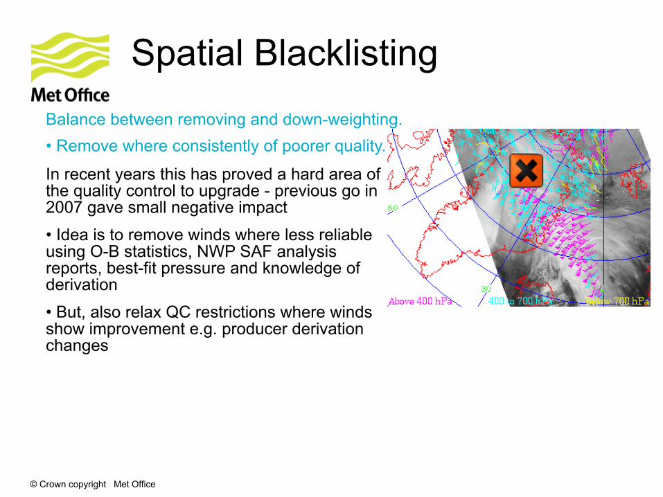
Spatial Blacklisting
In recent years this has proved a hard area of the quality control to upgrade - previous go in 2007 gave small negative impact • Idea is to remove winds where less reliable using O-B statistics, NWP SAF analysis reports, best-fit pressure and knowledge of derivation • But, also relax QC restrictions where winds show improvement e.g. producer derivation changes
Balance between removing and down-weighting. • Remove where consistently of poorer quality.
© Crown copyright Met Office
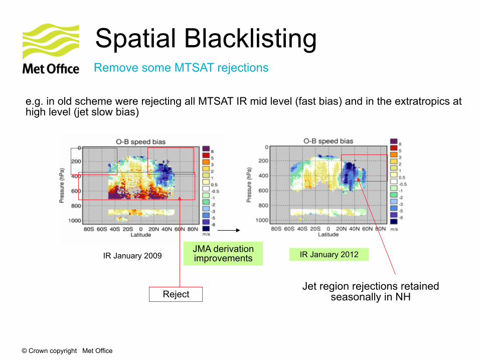
Spatial Blacklisting Remove some MTSAT rejections
e.g. in old scheme were rejecting all MTSAT IR mid level (fast bias) and in the extratropics at high level (jet slow bias)
IR January 2009 JMA derivation improvements
Reject Jet region rejections retained
seasonally in NH
IR January 2012

© Crown copyright Met Office
Spatial Blacklisting Other examples • Reset upper and lower pressure thresholds for all winds • Introduce topographic checks – mountainous regions • Implement CO2 slicing and WV intercept thresholds at mid level (Feature 2.9 AMV analysis reports) • Implement satellite zenith angle checks for all Geostationary • Retain MSG low level rejections over land NH (Feature 2.6 AMV analysis reports) • etc
Combined package of updated observation errors and spatial blacklisting – neutral to small positive impact on NWP Index • Operational since PS27, July 2011
vs Observations vs Analyses
Season 1 +0.1 +0.3
Season 2 +0.1 +0.2
© Crown copyright Met Office
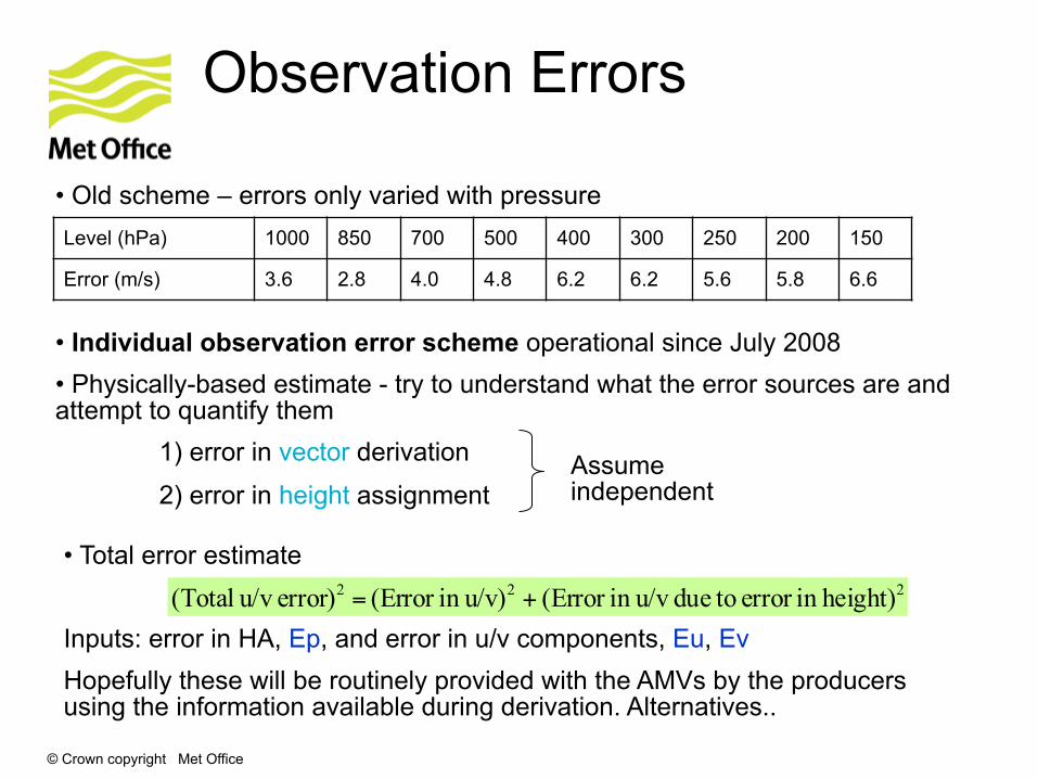
Observation Errors
• Individual observation error scheme operational since July 2008 • Physically-based estimate - try to understand what the error sources are and attempt to quantify them
1) error in vector derivation
2) error in height assignment
• Old scheme – errors only varied with pressure Level (hPa) 1000 850 700 500 400 300 250 200 150
Error (m/s) 3.6 2.8 4.0 4.8 6.2 6.2 5.6 5.8 6.6
Assume independent
• Total error estimate
Inputs: error in HA, Ep, and error in u/v components, Eu, Ev Hopefully these will be routinely provided with the AMVs by the producers using the information available during derivation. Alternatives..
222 height)in error todue u/vin (Error u/v)in (Error error) u/v (Total +=
© Crown copyright Met Office
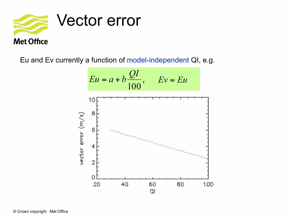
Vector error
Eu and Ev currently a function of model-independent QI, e.g.
,100QIbaEu += EuEv =
© Crown copyright Met Office
100 200 300 400 500 600 700 800 900
1000 -20 0 20 40 60
m/s
Pres
sure
(hPa
)
u component
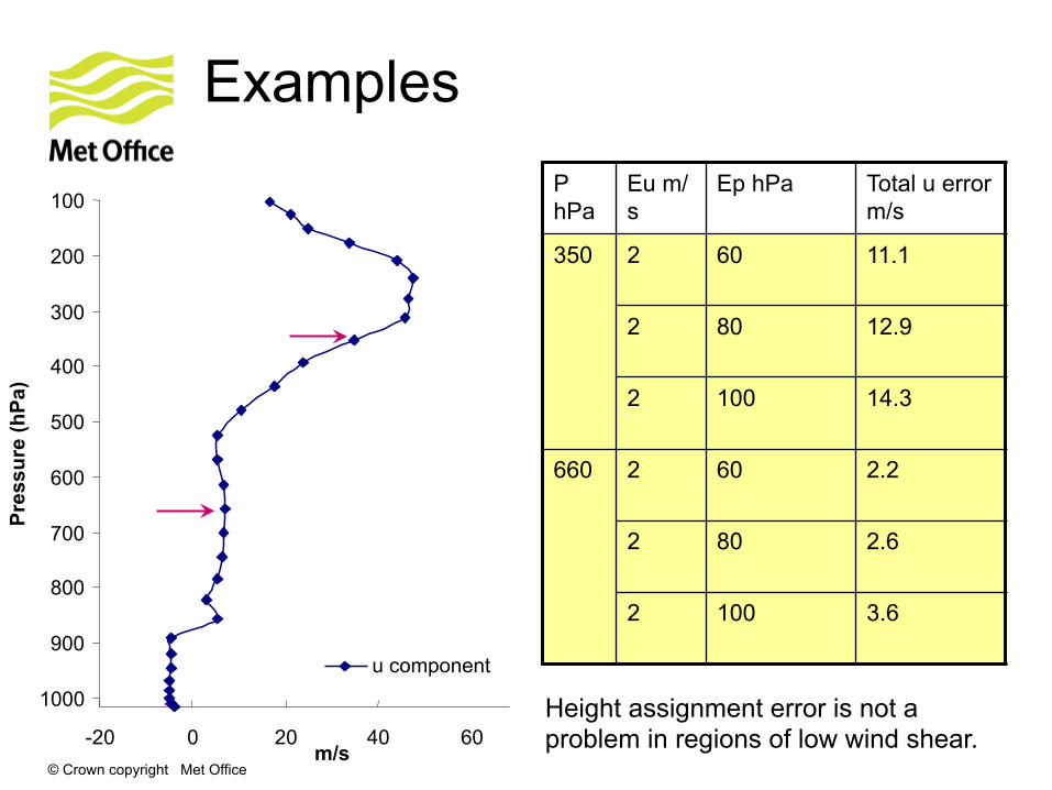
Examples P hPa
Eu m/s
Ep hPa Total u error m/s
350 2 60 11.1
2 80 12.9
2 100 14.3
660 2 60 2.2
2 80 2.6
2 100 3.6
Height assignment error is not a problem in regions of low wind shear.
© Crown copyright Met Office
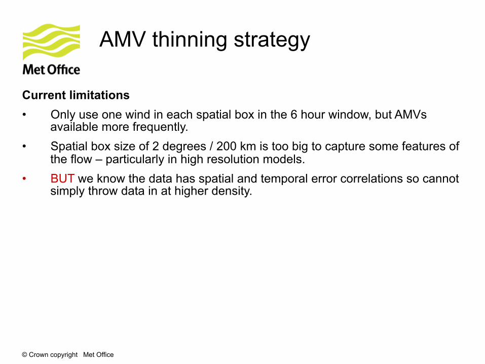
AMV thinning strategy •
Current limitations • Only use one wind in each spatial box in the 6 hour window, but AMVs
available more frequently. • Spatial box size of 2 degrees / 200 km is too big to capture some features of
the flow – particularly in high resolution models. • BUT we know the data has spatial and temporal error correlations so cannot
simply throw data in at higher density.
© Crown copyright Met Office
AMV thinning strategy •
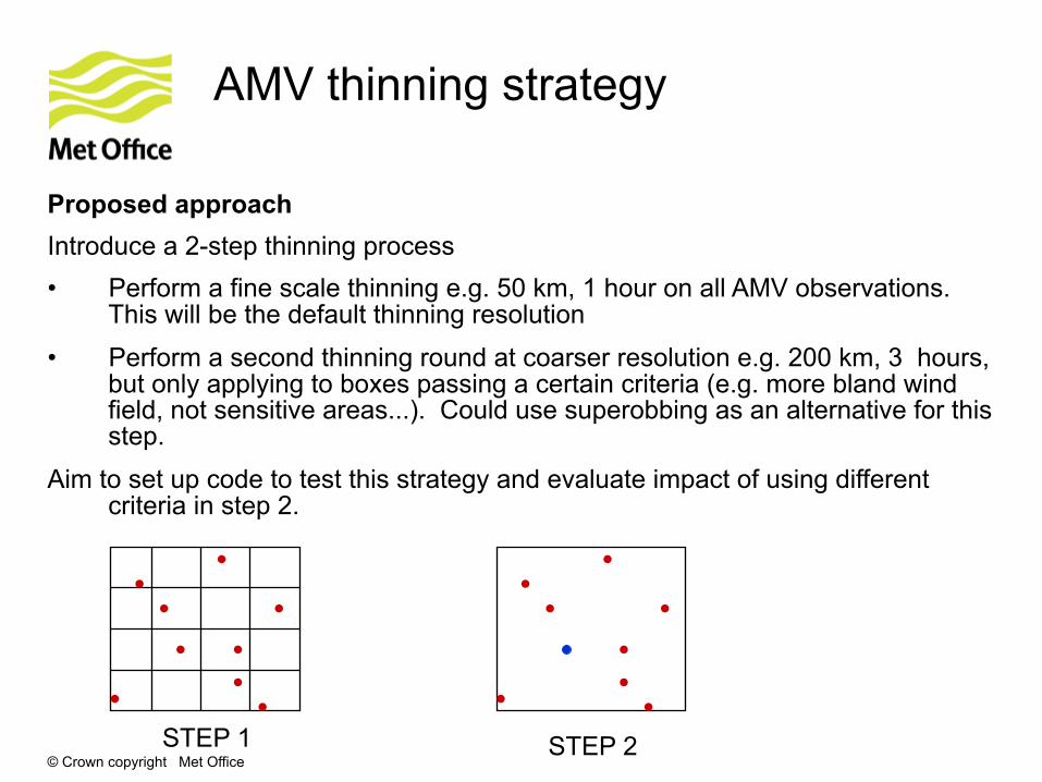
Proposed approach Introduce a 2-step thinning process • Perform a fine scale thinning e.g. 50 km, 1 hour on all AMV observations.
This will be the default thinning resolution • Perform a second thinning round at coarser resolution e.g. 200 km, 3 hours,
but only applying to boxes passing a certain criteria (e.g. more bland wind field, not sensitive areas...). Could use superobbing as an alternative for this step.
Aim to set up code to test this strategy and evaluate impact of using different criteria in step 2.
STEP 1 STEP 2
© Crown copyright Met Office
2. AMV thinning strategy •
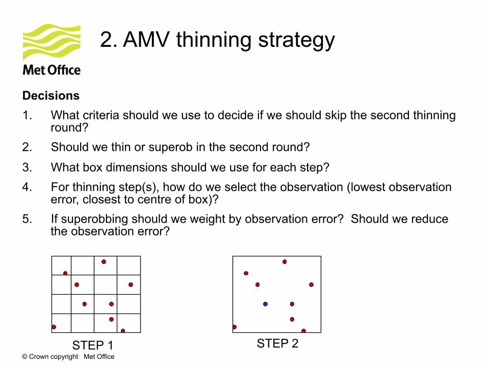
Decisions 1. What criteria should we use to decide if we should skip the second thinning
round? 2. Should we thin or superob in the second round?
3. What box dimensions should we use for each step? 4. For thinning step(s), how do we select the observation (lowest observation
error, closest to centre of box)? 5. If superobbing should we weight by observation error? Should we reduce
the observation error?
STEP 1 STEP 2
© Crown copyright Met Office © Crown copyright Met Office
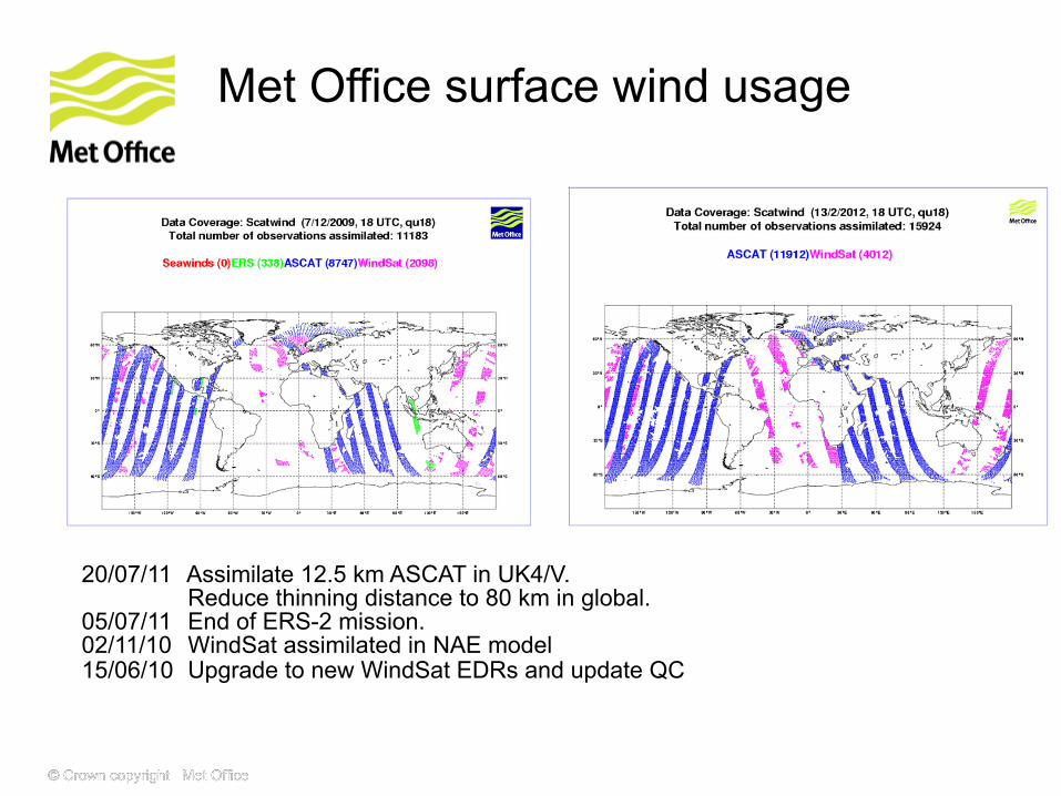
Met Office surface wind usage •
20/07/11 Assimilate 12.5 km ASCAT in UK4/V. Reduce thinning distance to 80 km in global.
05/07/11 End of ERS-2 mission. 02/11/10 WindSat assimilated in NAE model 15/06/10 Upgrade to new WindSat EDRs and update QC
© Crown copyright Met Office © Crown copyright Met Office
LeoGeo winds
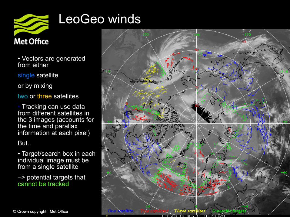
• Vectors are generated from either single satellite or by mixing two or three satellites • Tracking can use data from different satellites in the 3 images (accounts for the time and parallax information at each pixel) But.. • Target/search box in each individual image must be from a single satellite –> potential targets that cannot be tracked
© Crown copyright Met Office © Crown copyright Met Office
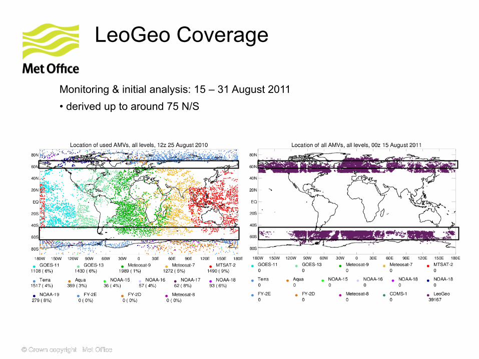
LeoGeo Coverage
Monitoring & initial analysis: 15 – 31 August 2011 • derived up to around 75 N/S
© Crown copyright Met Office © Crown copyright Met Office
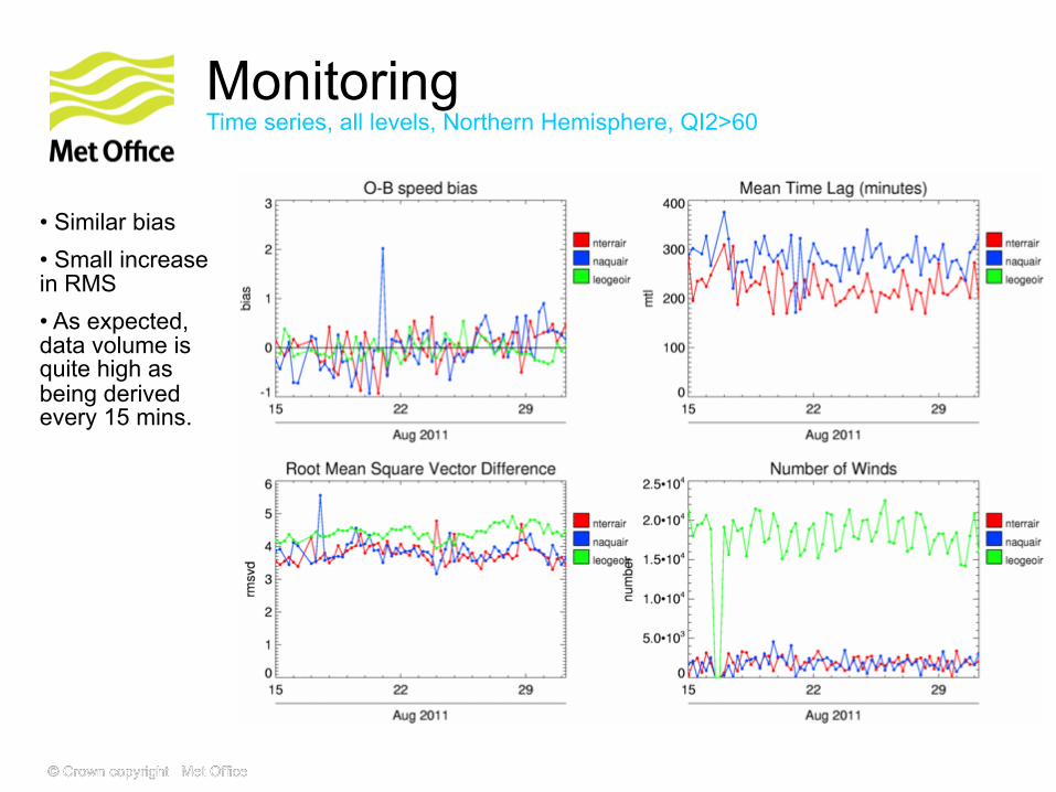
Monitoring Time series, all levels, Northern Hemisphere, QI2>60
• Similar bias • Small increase in RMS • As expected, data volume is quite high as being derived every 15 mins.
© Crown copyright Met Office © Crown copyright Met Office
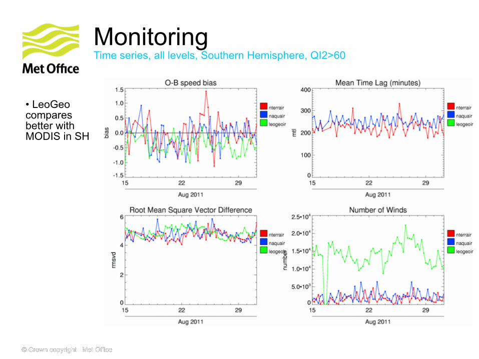
Monitoring Time series, all levels, Southern Hemisphere, QI2>60
• LeoGeo compares better with MODIS in SH