1

ALTERNATIVE SEASONAL ADJUSTMENT METHODS FOR AGGREGATE IRISH MACROECONOMIC DATA

John Lawlor Colm McCarthy*

Three distinct strands can be identified in the literature on seasonality. Economists have long been interested in removing high-frequency ‘noise’ from individual economic time series, or ‘de-seasonalising the data’ in common parlance. The second strand, on which an extensive technical literature has been developed over recent decades, treats seasonality as just one element to be encompassed in multivariate dynamic time series modelling, while a final strand seeks to model the economics of seasonality as the outcome of maximising behaviour by producing and consuming agents. See Brendstrup et al. (2002).

1. Introduction

Official statistical agencies around the world typically publish all main monthly and quarterly economic series in both primitive and seasonally-adjusted form, removing the high-frequency noise in the spirit of the first of the three strands. Sophisticated models and software packages have been developed to accomplish this task, the best-known of which are the empirical US Census Bureau’s X-11 package and its derivatives, and the model-based Tramo-Seats

*Corresponding: DKM Economic Consultants, 49 Dawson Street, Dublin 2: colm.mccarthy@davy.ie.

2

routines, developed by the Bank of Spain. Both are widely used by official agencies.

Aggregate economic time-series like GDP or industrial output can be deseasonalised by direct application of a seasonal adjustment procedure to the aggregate data. Alternatively the component series can be seasonally adjusted one by one and summed to give an estimate of the aggregate seasonally adjusted series. The two methods are called the direct and indirect methods respectively. In Ireland, the Central Statistics Office has been producing quarterly national accounts since Q1 1997, and seasonally adjusted data have been furnished since Q2 2003. The Central Statistics Office (CSO) has been preparing seasonal factors for the macro data using the direct method, and also publishes seasonally adjusted estimates for the sub-aggregates. In this paper, we will show that estimates using the indirect method (which are just the sums of the adjusted data for the sub-aggregates as published by the CSO) give radically different results in many cases. This is particularly noticeable where the seasonal adjustment is used to facilitate calculation of the underlying rate of growth. We show that the direct method often indicates one-period growth where the indirect alternative shows decline and vice versa. They will not give coincident estimates of the aggregate series except in special (and empirically infrequent) cases.

Thus if Y = C + I + G, and the seasonally adjusted series are denoted with an asterisk, the accounting identity in deseasonalised form Y*= C* + I* + G* will not hold in general, and a choice has to be made. The direct estimate Y* can be used, obtained through the application of the seasonal adjustment procedure directly to Y, or the sum C* + I* + G* can be used as the estimate of the deseasonalised aggregate, the indirect estimate.

There are two difficulties with the direct method. It will not, except in a special case, deliver consistent aggregation. In a quarterly macro model for example, the budget constraints and national accounting identities will be breached if all series, including the aggregates, are seasonally adjusted independently. (It is worth noting that, from Q1 2005, the CSO has moved from a fixed to a chain-linked methodology for the constant-price national accounts, and the application of chain-linking independently to the aggregate series also sacrifices consistent aggregation.) With direct seasonal adjustment, it can also happen that each (seasonally-adjusted) sub-component shows a decline in a particular month or quarter, but the aggregate rises according to the direct estimate. Additionally, there are grounds for expecting that the direct method will not deliver a satisfactory seasonal adjustment in many circumstances. But in a particular instance, it is possible that the two methods will deliver near-identical estimates of the seasonally adjusted aggregates. If all the component series have a similar additive seasonal pattern, the

3

best direct estimate of the aggregate will also be additive and the direct and indirect estimates will coincide. If the components have almost-additive patterns, the alternative adjustments for the aggregate should come close to coinciding, and such results have been reported. See Cabrero (2000), who finds generally small differences between direct and indirect adjustments for Spanish monetary aggregates, or Atuk and Ural (2002), who draw similar conclusions for Turkish monetary data.

But seasonal adjustment using standard packages such as X-12 or Tramo-Seats is in general a nonlinear transformation (even if the filter is linear) and will accordingly violate adding-up constraints, and may also yield very different deseasonalisations of aggregates as between direct and indirect adjustments. Results have been reported where the direct and indirect estimates differ significantly, for example Maravall (2002) on Japanese trade data. Intuitively, if the components of an aggregate have very different seasonal patterns (and they often will: the change in inventories, a GDP component, can hardly be expected to follow the seasonal pattern of investment, or consumption), the indirect method ought to be superior, since the direct approach, in these circumstances, is operating on an aggregate whose seasonal behaviour is a mish-mash of heterogeneous components. The number of sub-aggregates will typically be small, so reliance on some Central Limit Theorem notions about well-behaved aggregates is not appropriate. While there appear to be no definitive theoretical or Monte Carlo results pointing to the superiority of either method, most national statistical offices favour the indirect method, as does Eurostat. See Planas and Campolongo (2003), who conclude

…when series have similar patterns, direct adjustment is more accurate…, but they continue …when series have dissimilar patterns, indirect adjustment is more accurate than direct adjustment, both for final and revision errors and regardless whether the adjustment is model-based or X11-based.

Simple linear structures for the filter applied to the component series, which can be shown to imply coincidence of the direct and indirect estimates where all component filters have the same lag length, are not frequently encountered. The UK’s Government Statistical Service (1996) found, in a trawl of UK agencies conducting seasonal adjustment, mainly using variants of X-11, that 949 out of 1,463 monthly series had multiplicative patterns, and so did 1,621 out of 2,464 quarterly series.

As with the quarterly macro aggregates, the CSO also uses the direct method for monthly series such as the Retail Sales Index and the Industrial Production Index. The construction of these aggregates is more complex than is the case with the national accounts, but it appears that direct and indirect seasonal adjustment methods also give materially different answers, in some cases, for these important monthly data.

4

For the national accounts, and also for retail sales and industrial production, it is clear that the sub-aggregates do not share what Planas and Campolongo call ‘similar patterns’. While it is not possible to argue that the Irish CSO’s use of the direct method will be inferior in all cases, the technical literature supports a presumption that this will be the case, and we conclude that consideration should be given to a change of methodology for the seasonal adjustment of the key aggregate series.

The quarterly National Income and Expenditure data for Ireland is

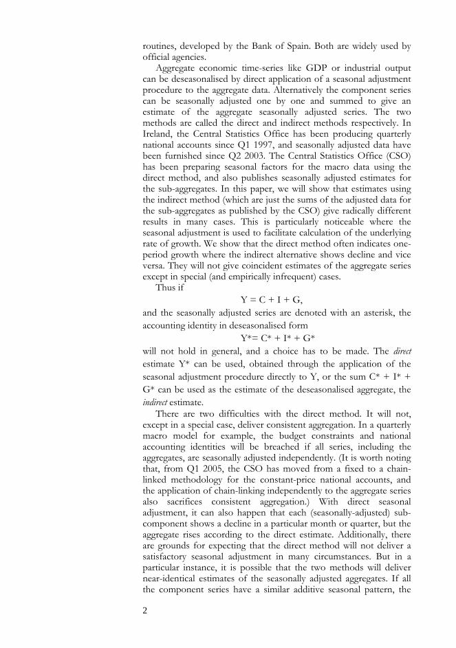
still quite a short series, commencing in Q1 1997. In this paper, we have studied the data up to Q4 2004 (32 observations). Because of the short data-run, the CSO re-estimates the SA factors with each new observation. Appendix A sets out the SA data per the CSO.1 The following charts show the figures under the direct and indirect approaches graphically.

2. Quarterly National Accounts

Figure 1: GDP SA Direct Versus Indirect Approach

14,000

16,000

18,000

20,000

22,000

24,000

26,000

28,000

1997

Q1

1997

Q3

1998

Q1

1998

Q3

1999

Q1

1999

Q3

2000

Q1

2000

Q3

2001

Q1

2001

Q3

2002

Q1

2002

Q3

2003

Q1

2003

Q3

2004

Q1

2004

Q3

GDP Direct GDP Indirect

1 A complication with calculating GDP/GNP SA under the indirect approach is the treatment of the statistical discrepancy, which arises from the difference in GDP calculated using the output and expenditure methods, and is one of the components of aggregate GDP in the nsa series. The CSO does not report a SA statistical discrepancy, and it is not necessary using the direct method. The series can be tested for a seasonal pattern, and if it has one it should be included in our indirect aggregation. Otherwise, it should be included unadjusted. X12 ARIMA, a development of the X11 ARIMA package used by the CSO, finds a seasonal pattern in the statistical discrepancy series to Q4 2004 and thus we include this series SA in our aggregation.

5

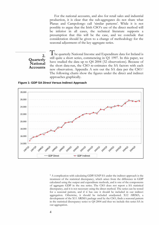
Figure 2: GNP SA Direct Versus Indirect Approach

12,000

13,000

14,000

15,000

16,000

17,000

18,000

19,000

20,000

21,000

1997

Q1

1997

Q3

1998

Q1

1998

Q3

1999

Q1

1999

Q3

2000

Q1

2000

Q3

2001

Q1

2001

Q3

2002

Q1

2002

Q3

2003

Q1

2003

Q3

2004

Q1

2004

Q3

GNP Direct GNP Indirect

The two alternative estimates of both the GDP and GNP series

clearly differ. There are cases, which we consider below, where one approach shows an increase in quarterly GDP/GNP while the other shows a decrease. Table 1 sets out the quarterly percentage changes in the SA GDP and GNP figures, and the difference between the two approaches. This is the statistic of most interest when the series are released, and which attracts the greatest attention from analysts and commentators. We calculate the average of the absolute quarterly percentage change under each approach. The results indicate:

1. The absolute average difference in the SA quarterly growth rate between the two approaches is no less than 2.08 per cent (per quarter, 8.6 per cent annualised) for the GNP series, and 1.43 per cent (5.9 per cent annualised) for the GDP series.

2. For GNP, 28 out of 31 cases show a difference of greater than 1 per cent in the quarter-on-quarter growth rate (corresponding to over 4 per cent annualised); for GDP the same is true in 22 out of 31 cases.

3. The difference between the direct and indirect approaches is greater for GNP than for GDP.2

2 This ranking is not stable as new data are added. Carrying out the exercise on seasonally adjusted data to Q2 2004 (just two observations less than used here) gave greater differences in the GDP series. Note that the CSO re-estimate the entire SA series with each new observation.

6

4. There are 9 quarters out of 31 where the GNP figure rose under one approach but fell under the other; for GDP there are 6 such cases.

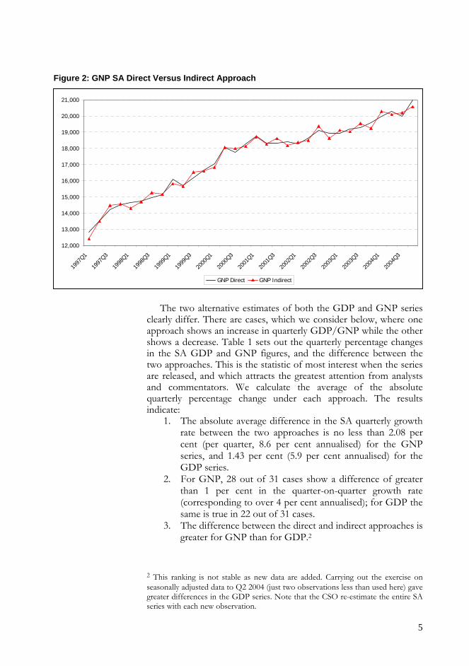
Table 1: Quarterly Percentage Changes in SA GDP and GNP

GDP GNP

Difference

in Difference

in

Direct Indirect Percentage

Points Direct Indirect Percentage

Points % % % % % %

1997Q2 3.59 6.85 3.25 5.70 8.76 3.06

1997Q3 0.58 1.74 1.16 5.10 7.30 2.19

1997Q4 3.91 2.82 -1.09 2.00 0.55 -1.45

1998Q1 2.50 -0.24 -2.74 0.89 -1.81 -2.70

1998Q2 1.36 4.11 2.75 0.59 2.83 2.24

1998Q3 2.52 3.24 0.72 1.59 3.75 2.16

1998Q4 -0.81 -1.59 -0.78 1.04 -0.65 -1.68

1999Q1 7.11 5.00 -2.11 6.55 4.32 -2.23

1999Q2 -1.09 0.85 1.93 -2.59 -0.94 1.64

1999Q3 6.16 6.93 0.78 3.24 5.50 2.26

1999Q4 1.93 0.71 -1.22 2.79 0.44 -2.35

2000Q1 0.71 -0.02 -0.72 2.40 1.46 -0.95

2000Q2 3.53 4.72 1.19 5.93 7.27 1.35

2000Q3 2.14 2.59 0.44 -1.75 -0.42 1.32

2000Q4 3.73 2.37 -1.36 2.94 0.77 -2.17

2001Q1 0.92 1.67 0.74 2.66 3.21 0.55

2001Q2 -0.36 -0.53 -0.17 -2.24 -2.37 -0.13

2001Q3 1.18 1.93 0.74 0.03 1.88 1.85

2001Q4 -0.04 -1.64 -1.60 0.39 -2.32 -2.71

2002Q1 3.87 5.73 1.87 -0.75 1.11 1.86

2002Q2 0.32 -0.89 -1.21 2.01 0.68 -1.34

2002Q3 2.68 3.64 0.96 2.45 4.70 2.26

2002Q4 0.46 -1.09 -1.55 -0.82 -3.83 -3.01

2003Q1 0.04 2.13 2.09 -0.09 2.63 2.72

2003Q2 1.90 0.19 -1.71 1.51 -0.48 -1.99

2003Q3 -1.52 -0.48 1.03 0.50 2.68 2.18

2003Q4 4.58 3.21 -1.37 1.49 -1.52 -3.01

2004Q1 1.28 3.55 2.26 1.99 5.44 3.45

2004Q2 0.87 -1.21 -2.08 1.48 -0.95 -2.44

2004Q3 -1.41 -0.21 1.20 -1.49 0.50 1.99

2004Q4 2.01 0.47 -1.54 5.07 1.87 -3.19 Average Absolute 2.10 2.33 1.43 2.26 2.68 2.08 Volatility Measure 2.94 3.30 2.48 4.42

7

The direct and indirect methods give, in summary, dramatically

different estimates, and the choice between them is material for these data. The difference arises because different seasonal patterns apply to the various component series making up GDP/GNP. We estimate, using X-12 ARIMA, that Personal Consumption, Government Consumption and Imports have linear seasonal patterns but with differing lag lengths in the moving averages chosen, while Fixed Capital Formation and Exports have multiplicative patterns.

The volatility measure shown is the mean of the sequential absolute difference in the growth rates. For both GDP and GNP the indirect approach increases the volatility of these quarterly growth rates. The Irish macro aggregates, seasonally adjusted as per the CSO’s existing (direct) methodology, appear to be noticeably volatile anyway, see McCarthy (2004). If the indirect approach is to be preferred, this problem is even greater. For real GNP, the quarterly (sequential) growth rate (computed via the indirect method) differs an absolute 4.42 per cent on average from the figure a quarter earlier.

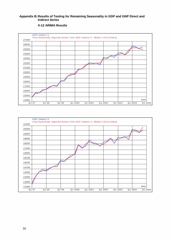
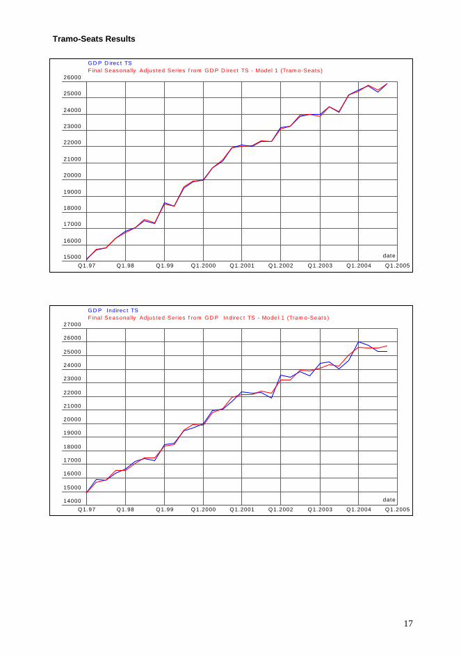
A “good” seasonal adjustment procedure should yield a series with no substantial remaining seasonality. We ran the alternative SA GDP and GNP figures from CSO through the X-12 ARIMA and Tramo-Seats packages, to see whether there was any discernible seasonal pattern left in the numbers. One would not expect any in the directly seasonally adjusted series, since these were arrived at by simply seasonally adjusting the aggregate NSA series. Some pattern might remain in the indirect seasonally adjusted series.

X-12 ARIMA found no remaining seasonality in the directly adjusted series, not surprising since this is the package used by CSO, but did find it in both indirectly adjusted series. Tramo-Seats found residual seasonality in the GDP direct and indirect series, but did not find it in either version of the GNP series. This suggests that the CSO’s current choice of seasonal adjustment factors for the macro components could perhaps be improved on, although it must be recalled that the data series is short. The results of this exercise are given graphically in Appendix B.

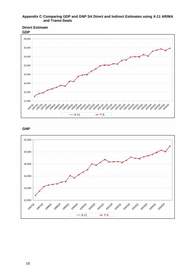
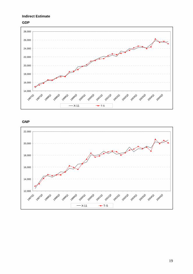
The results also illustrate that X-11/X-12 and Tramo-Seats sometimes give different seasonal factors. This can be demonstrated further by estimating the SA GDP and GNP by Tramo-Seats, and comparing the results with the figures estimated by the CSO (using X-11 ARIMA). The results are given graphically in Appendix C. As can be seen, the results are very close when seasonally adjusting GDP and GNP directly, but substantial differences arise when using the indirect approach. The aggregation of the RSI, from 15 constituent business sectors, is more complicated than that for GDP/GNP. Starting with the actual turnover in each business sector, a number of steps are followed:

3. The Retail Sales

Index

8

1. Trading Day and Trading Week: Sales in each month vary

with the number of trading days and weeks. The CSO generates “Standardised months”, which have the same number of weeks, and the same number of Mondays, Tuesdays, etc.

2. The RSI turnover index is calculated using a modified Laspèyres index based on a set of fixed seasonal weights. The relative weight of each sector varies from month to month, and a set of current weights is used (“updated values”), based on the change in turnover in each sector in the last twelve months.

The formulae for the individual business sectors and aggregate RSIs are:

Individual RSI = [Wm-1(Tm/Tm-1)/ W0] x 100

Aggregate RSI = [Σ(Wm-1(Tm/Tm-1))/ ΣW0] x 100

Where

0 and 1−m are the base weights and updated weights (“updated values”) respectively, and

W W

m and 1−m are turnover values for the current and last period respectively.

T T

0 = Base period (i.e. equivalent month in the base year 2000) m = current month m-1 = same month last year.

3. The turnover index is converted to a volume index using indices for each business sector derived from the CPI.

4. The series are then seasonally adjusted, with the SA factors updated twice-yearly. The set of factors used here is based on the seasonal pattern from January 1999 to April 2004.

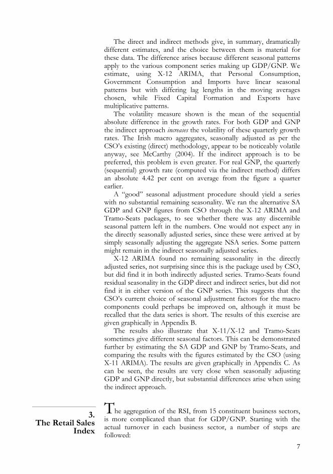
Because of the method of calculation, it is not straightforward to compare the SA aggregate series generated by the direct and indirect approaches. We have taken a simple approach of calculating the average of the individual SA volume indices, weighted by the base weights, and comparing the monthly change in the resultant average with the monthly change in the aggregate SA volume index as calculated by the CSO. This should identify inconsistencies between the direct and indirect approaches to estimating the aggregate SA volume index. Figure 3 below shows the two series graphically.

9

Figure 3: Weighted Average of SA Volume Indices Versus Aggregate SA Volume Index per CSO

90

95

100

105

110

115

Jan-

00

Mar-0

0

May-0

0Ju

l-00

Sep-

00

Nov-0

0

Jan-

01

Mar-0

1

May-0

1Ju

l-01

Sep-

01

Nov-0

1

Jan-

02

Mar-0

2

May-0

2Ju

l-02

Sep-

02

Nov-0

2

Jan-

03

Mar-0

3

May-0

3Ju

l-03

Sep-

03

Nov-0

3

Jan-

04

Mar-0

4

May-0

4Ju

l-04

Sep-

04

Nov-0

4

Jan-

05

W eighted Average sa Volume Index All Businesses SA Volume Index per CSO

The CSO series is on average a higher number than the series we calculated, which is to be expected, as the CSO series would give greater weight to the sectors with higher sales over time, thus boosting growth in the index.

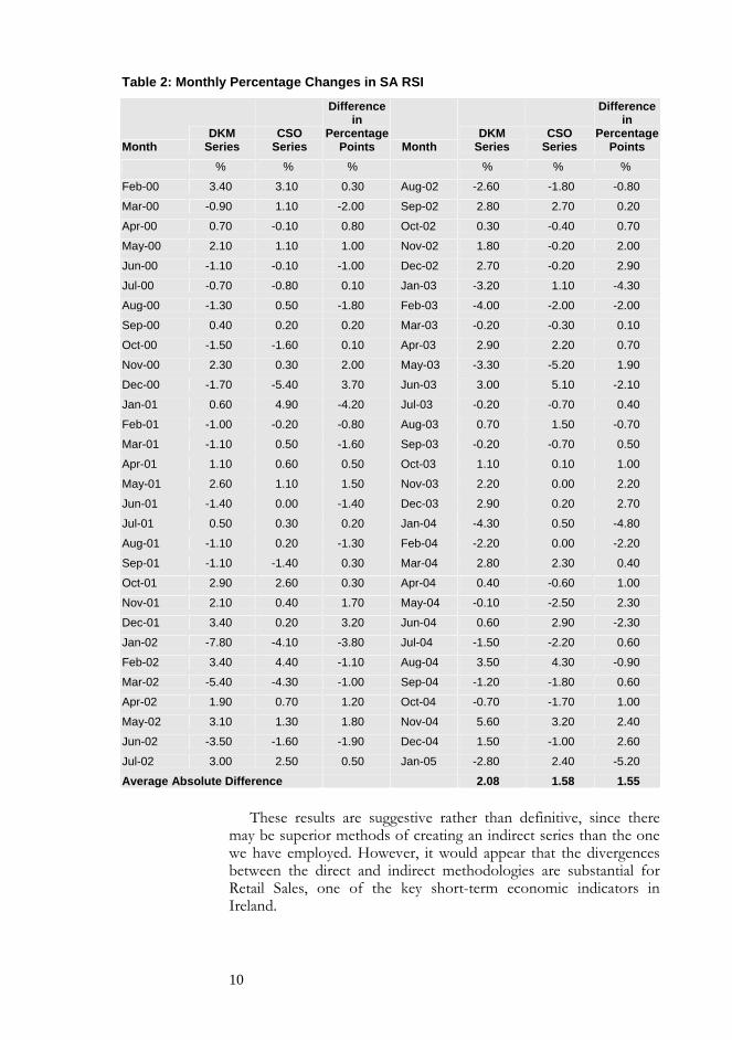
Table 2 overleaf sets out the monthly percentage changes in the two series since 2000. We calculate (1) the average of the absolute monthly changes, and (2) the average of the absolute differences between the two approaches. The results indicate that there is slightly more variability in the series we have calculated, and the average absolute difference in the growth rates in the two series is 1.55 per cent.

Comparing the two series also highlights a number of cases where the weighted average of the individual series indicates a reduction in overall retail volumes, while the aggregate series per the CSO indicate an increase, or vice versa. This occurs in no less than 16 cases out of 60.

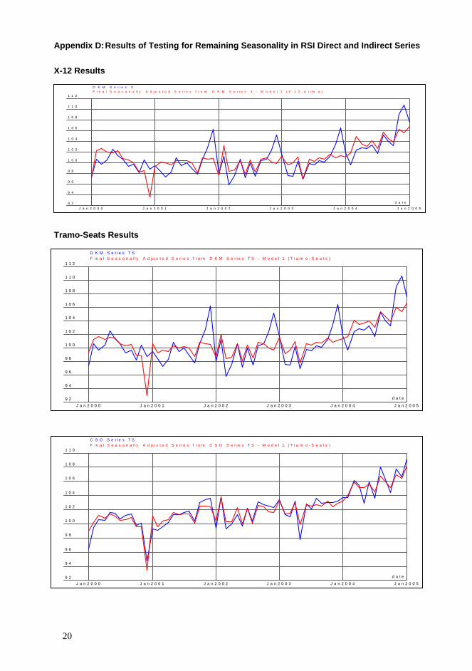
We also carried out an exercise running the two series through X-12 ARIMA and Tramo-Seats, to see whether there was any discernible seasonal pattern left in the numbers. One would not expect any remaining SA pattern in the directly seasonally adjusted series, since this was arrived at by simply seasonally adjusting the aggregate nsa series. Some pattern might remain in the series generated indirectly, and X-12 found that seasonality was “probably present” in this series; Tramo-Seats found some surviving seasonality in both series. The results are summarised graphically in Appendix D.

10

Table 2: Monthly Percentage Changes in SA RSI

Month DKM

Series CSO

Series

Difference in

PercentagePoints Month

DKM Series

CSO Series

Difference in

Percentage Points

% % % % % %

Feb-00 3.40 3.10 0.30 Aug-02 -2.60 -1.80 -0.80

Mar-00 -0.90 1.10 -2.00 Sep-02 2.80 2.70 0.20

Apr-00 0.70 -0.10 0.80 Oct-02 0.30 -0.40 0.70

May-00 2.10 1.10 1.00 Nov-02 1.80 -0.20 2.00

Jun-00 -1.10 -0.10 -1.00 Dec-02 2.70 -0.20 2.90

Jul-00 -0.70 -0.80 0.10 Jan-03 -3.20 1.10 -4.30

Aug-00 -1.30 0.50 -1.80 Feb-03 -4.00 -2.00 -2.00

Sep-00 0.40 0.20 0.20 Mar-03 -0.20 -0.30 0.10

Oct-00 -1.50 -1.60 0.10 Apr-03 2.90 2.20 0.70

Nov-00 2.30 0.30 2.00 May-03 -3.30 -5.20 1.90

Dec-00 -1.70 -5.40 3.70 Jun-03 3.00 5.10 -2.10

Jan-01 0.60 4.90 -4.20 Jul-03 -0.20 -0.70 0.40

Feb-01 -1.00 -0.20 -0.80 Aug-03 0.70 1.50 -0.70

Mar-01 -1.10 0.50 -1.60 Sep-03 -0.20 -0.70 0.50

Apr-01 1.10 0.60 0.50 Oct-03 1.10 0.10 1.00

May-01 2.60 1.10 1.50 Nov-03 2.20 0.00 2.20

Jun-01 -1.40 0.00 -1.40 Dec-03 2.90 0.20 2.70

Jul-01 0.50 0.30 0.20 Jan-04 -4.30 0.50 -4.80

Aug-01 -1.10 0.20 -1.30 Feb-04 -2.20 0.00 -2.20

Sep-01 -1.10 -1.40 0.30 Mar-04 2.80 2.30 0.40

Oct-01 2.90 2.60 0.30 Apr-04 0.40 -0.60 1.00

Nov-01 2.10 0.40 1.70 May-04 -0.10 -2.50 2.30

Dec-01 3.40 0.20 3.20 Jun-04 0.60 2.90 -2.30

Jan-02 -7.80 -4.10 -3.80 Jul-04 -1.50 -2.20 0.60

Feb-02 3.40 4.40 -1.10 Aug-04 3.50 4.30 -0.90

Mar-02 -5.40 -4.30 -1.00 Sep-04 -1.20 -1.80 0.60

Apr-02 1.90 0.70 1.20 Oct-04 -0.70 -1.70 1.00

May-02 3.10 1.30 1.80 Nov-04 5.60 3.20 2.40

Jun-02 -3.50 -1.60 -1.90 Dec-04 1.50 -1.00 2.60

Jul-02 3.00 2.50 0.50 Jan-05 -2.80 2.40 -5.20

Average Absolute Difference 2.08 1.58 1.55

These results are suggestive rather than definitive, since there may be superior methods of creating an indirect series than the one we have employed. However, it would appear that the divergences between the direct and indirect methodologies are substantial for Retail Sales, one of the key short-term economic indicators in Ireland.

11

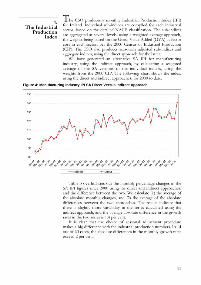
The CSO produces a monthly Industrial Production Index (IPI) for Ireland. Individual sub-indices are compiled for each industrial sector, based on the detailed NACE classification. The sub-indices are aggregated at several levels, using a weighted average approach, the weights being based on the Gross Value Added (GVA) at factor cost in each sector, per the 2000 Census of Industrial Production (CIP). The CSO also produces seasonally adjusted sub-indices and aggregate indices, using the direct approach for the latter.

4. The Industrial

Production Index

We have generated an alternative SA IPI for manufacturing industry, using the indirect approach, by calculating a weighted average of the SA versions of the individual indices, using the weights from the 2000 CIP. The following chart shows the index, using the direct and indirect approaches, for 2000 to date.

Figure 4: Manufacturing Industry IPI SA Direct Versus Indirect Approach

80

90

100

110

120

130

140

150

Jan-

00

Mar-0

0

May-0

0Ju

l-00

Sep-

00

Nov-0

0

Jan-

01

Mar-0

1

May-0

1Ju

l-01

Sep-

01

Nov-0

1

Jan-

02

Mar-0

2

May-0

2Ju

l-02

Sep-

02

Nov-0

2

Jan-

03

Mar-0

3

May-0

3Ju

l-03

Sep-

03

Nov-0

3

Jan-

04

Mar-0

4

May-0

4Ju

l-04

Indirect Direct

Table 3 overleaf sets out the monthly percentage changes in the

SA IPI figures since 2000 using the direct and indirect approaches, and the difference between the two. We calculate (1) the average of the absolute monthly changes, and (2) the average of the absolute differences between the two approaches. The results indicate that there is slightly more variability in the series calculated using the indirect approach, and the average absolute difference in the growth rates in the two series is 1.4 per cent.

It is clear that the choice of seasonal adjustment procedure makes a big difference with the industrial production numbers. In 14 out of 60 cases, the absolute differences in the monthly growth rates exceed 2 per cent.

12

Table 3: Monthly Percentage Changes in SA Manufacturing Industry IPI

Month Indirect Direct

Difference in Percentage

Points Month Indirect Direct

Difference in Percentage

Points % % % % % %

Feb-00 3.60 -0.10 3.70 Aug-02 1.20 0.40 0.80

Mar-00 5.30 2.00 3.30 Sep-02 1.40 1.00 0.40

Apr-00 9.40 10.70 -1.40 Oct-02 -3.00 -3.60 0.60

May-00 -1.00 0.30 -1.40 Nov-02 0.40 1.70 -1.30

Jun-00 -0.50 0.50 -1.00 Dec-02 -7.60 -9.70 2.10

Jul-00 4.20 4.60 -0.30 Jan-03 8.40 10.90 -2.50

Aug-00 -2.50 -2.80 0.30 Feb-03 3.50 3.50 0.00

Sep-00 1.10 2.00 -0.90 Mar-03 -2.70 -3.30 0.70

Oct-00 4.40 6.30 -2.00 Apr-03 2.40 1.80 0.60

Nov-00 3.80 4.40 -0.60 May-03 0.10 1.50 -1.40

Dec-00 4.90 -0.80 5.70 Jun-03 -0.70 -1.00 0.30

Jan-01 -4.90 -0.80 -4.10 Jul-03 3.00 3.10 -0.10

Feb-01 9.20 8.80 0.40 Aug-03 5.10 7.00 -1.80

Mar-01 -5.50 -7.40 1.90 Sep-03 -11.30 -13.10 1.80

Apr-01 0.70 1.30 -0.60 Oct-03 14.90 15.30 -0.40

May-01 -12.70 -12.30 -0.30 Nov-03 -0.20 -0.40 0.20

Jun-01 10.80 10.50 0.30 Dec-03 -4.50 -5.80 1.20

Jul-01 -7.90 -5.30 -2.60 Jan-04 -3.90 -1.00 -3.00

Aug-01 8.10 6.60 1.50 Feb-04 0.50 0.50 0.00

Sep-01 -1.30 -2.70 1.40 Mar-04 1.10 -0.40 1.50

Oct-01 -2.80 -4.00 1.20 Apr-04 6.10 3.90 2.30

Nov-01 0.10 1.80 -1.70 May-04 -7.70 -4.60 -3.00

Dec-01 15.70 10.20 5.60 Jun-04 -0.20 -0.60 0.40

Jan-02 -1.90 1.60 -3.50 Jul-04 16.40 14.90 1.40

Feb-02 -6.30 -4.80 -1.60 Aug-04 -19.50 -18.70 -0.80

Mar-02 13.90 11.40 2.50 Sep-04 6.90 5.20 1.70

Apr-02 -10.50 -9.70 -0.80 Oct-04 2.10 2.10 0.00

May-02 7.70 8.40 -0.80 Nov-04 -2.60 -2.10 -0.50

Jun-02 2.90 2.50 0.40 Dec-04 3.80 3.60 0.20

Jul-02 -6.40 -6.10 -0.30 Jan-05 2.20 4.30 -2.10

Average Absolute Difference 5.22 4.93 1.42

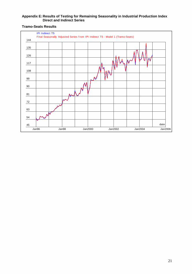
We also carried out an exercise running the two SA IPI series through X-12 ARIMA and Tramo-Seats, to see whether there was any discernible seasonal pattern left in the numbers. We considered the two series from January 1996 to date, and did not test for trading day or other factors. One would not expect any remaining SA pattern in the directly seasonally adjusted series, since these were arrived at by simply seasonally adjusting the aggregate nsa series. Some pattern might remain in the indirect seasonally adjusted series. Neither X-12 nor Tram-Seats found any remaining seasonality in the

13

direct series, but Tramo-Seats found seasonality in the indirect series (see Appendix E).

We have compared direct and indirect approaches to the seasonal

adjustment of Irish macroeconomic series published by the CSO. The presumption in the literature is that the indirect method is likely to be preferred in most real-world situations, but it is an empirical question whether it makes any great practical difference. Our results indicate that it makes a very big difference indeed, with one-period growth rates frequently changing sign, for example. It is clear that the component series have markedly differing seasonal patterns, and that this is contributing to the large differences between the two approaches. These are the circumstances in which the indirect method is likely to give a better adjustment.

5. Discussion of

Results and Conclusions

However the indirect estimates have problems too, including residual seasonality in some cases. There are also trends to be noted in the relationship between the direct and indirect adjustments. For example, with the macro aggregates (and this is true for both GDP and GNP), the gap between the two drifts steadily upwards for the Q1 factors, compensated by a steady downtrend for Q2. With short series, there can always be problems with end-points, and the differences between the two approaches tended to be larger for some quarters in 2004, the final year of the sample. Formal diagnostic tests for seasonal adjustment of aggregated series are discussed in Hood and Findley (2004).

But the fact that the indirect estimation of seasonal factors does not purge the Irish macro data of apparently extreme volatility does not count against the approach; rather it suggests that the source of the extreme volatility lies elsewhere. Given the big differences between direct and indirect estimates our conclusion is that it is desirable to take a fresh look at alternative seasonal adjustment procedures for the key aggregate macro series.

14

REFERENCES

ATUK, O. and B. P. URAL, 2002. “Seasonal Adjustment in Economic Time Series”, Central Bank of Turkey Discussion Paper 2002/1.

BRENDSTRUP, B., S. HYLLEBERG, M. NIELSEN, L. SKIPPER and L. STENTOFT, 2001. “Seasonality in Economic Models”, University of Aarhus, Dept. of Economics, WP No. 2001-16.

CABRERO, A., 2000. “Seasonal Adjustment in Economic Time Series: The Experience of the Banco de Espana”, Bank of Spain Working Paper 0002.

GOVERNMENT STATISTICAL SERVICE (UK) 1996. “Report of the Task Force on Seasonal Adjustment”, Methodology Series #2, January.

HOOD, C. and D. FINDLEY, 2004. “Comparing Direct and Indirect Seasonal Adjustments of Aggregate Series”, US Census Bureau, Washington DC.

MARAVALL, A., 2002. “An Application of Tramo-Seats: Automatic Procedure and Sectoral Aggregation”, Bank of Spain.

McCARTHY, C., 2004. “Volatility in Quarterly Irish Macro Data”, ESRI Quarterly Economic Commentary, Spring, pp. 81-89.

PLANAS, C. and F. CAMPOLONGO, 2003. “The Seasonal Adjustment of Contemporaneously Aggregated Series”, Luxembourg: Eurostat Working Papers and Studies.

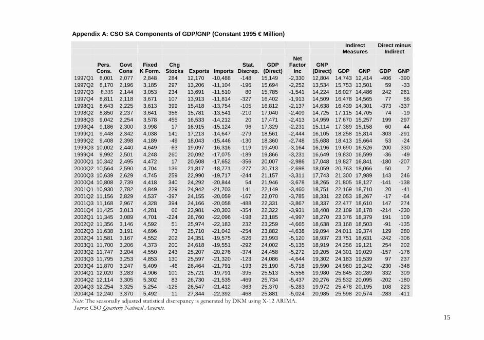
Appendix A: CSO SA Components of GDP/GNP (Constant 1995 € Million)

Indirect

Measures Direct minus

Indirect

Pers. Cons.

Govt Cons

Fixed K Form.

Chg Stocks Exports Imports

Stat. Discrep.

GDP (Direct)

Net Factor

Inc GNP

(Direct) GDP GNP GDP GNP 1997Q1 8,001 2,077 2,848 284 12,170 -10,488 -148 15,149 -2,330 12,804 14,743 12,414 -406 -3901997Q2 8,170 2,196 3,185 297 13,206 -11,104 -196 15,694 -2,252 13,534 15,753 13,501 59 -331997Q3 8,335 2,144 3,053 234 13,691 -11,510 80 15,785 -1,541 14,224 16,027 14,486 242 2611997Q4 8,811 2,118 3,671 107 13,913 -11,814 -327 16,402 -1,913 14,509 16,478 14,565 77 561998Q1 8,643 2,225 3,613 399 15,418 -13,754 -105 16,812 -2,137 14,638 16,439 14,301 -373 -3371998Q2 8,850 2,237 3,641 356 15,781 -13,541 -210 17,040 -2,409 14,725 17,115 14,705 74 -191998Q3 9,042 2,254 3,578 455 16,533 -14,212 20 17,471 -2,413 14,959 17,670 15,257 199 2971998Q4 9,186 2,300 3,998 17 16,915 -15,124 96 17,329 -2,231 15,114 17,389 15,158 60 441999Q1 9,448 2,342 4,038 141 17,213 -14,647 -279 18,561 -2,444 16,105 18,258 15,814 -303 -2911999Q2 9,408 2,398 4,189 -49 18,043 -15,446 -130 18,360 -2,748 15,688 18,413 15,664 53 -241999Q3 10,002 2,440 4,649 -63 19,097 -16,316 -119 19,490 -3,164 16,196 19,690 16,526 200 3301999Q4 9,992 2,501 4,248 260 20,092 -17,075 -189 19,866 -3,231 16,649 19,830 16,599 -36 -492000Q1 10,342 2,495 4,472 17 20,508 -17,652 -356 20,007 -2,986 17,048 19,827 16,841 -180 -2072000Q2 10,564 2,590 4,704 136 21,817 -18,771 -277 20,713 -2,698 18,059 20,763 18,066 50 72000Q3 10,639 2,629 4,745 259 22,990 -19,717 -244 21,157 -3,311 17,743 21,300 17,989 143 2462000Q4 10,808 2,739 4,418 340 24,292 -20,844 54 21,946 -3,678 18,265 21,805 18,127 -141 -1382001Q1 10,930 2,782 4,849 229 24,942 -21,703 141 22,149 -3,460 18,751 22,169 18,710 20 -412001Q2 11,156 2,829 4,537 -397 24,155 -20,059 -167 22,070 -3,785 18,331 22,053 18,267 -17 -642001Q3 11,168 2,967 4,328 394 24,166 -20,058 -488 22,331 -3,867 18,337 22,477 18,610 147 2742001Q4 11,425 3,013 4,281 66 23,981 -20,303 -354 22,322 -3,931 18,408 22,109 18,178 -214 -2302002Q1 11,345 3,089 4,701 -224 26,760 -22,096 -198 23,185 -4,997 18,270 23,376 18,379 191 1092002Q2 11,356 3,146 4,592 51 25,974 -22,183 232 23,259 -4,665 18,638 23,168 18,503 -91 -1352002Q3 11,638 3,191 4,696 73 25,710 -21,042 -254 23,882 -4,638 19,094 24,011 19,374 129 2802002Q4 11,581 3,167 4,552 202 24,351 -19,575 -526 23,993 -5,120 18,937 23,751 18,631 -242 -3062003Q1 11,700 3,206 4,373 200 24,618 -19,551 -292 24,002 -5,135 18,919 24,256 19,121 254 2022003Q2 11,747 3,204 4,550 243 25,207 -20,276 -374 24,458 -5,272 19,205 24,301 19,029 -157 -1762003Q3 11,795 3,253 4,853 130 25,597 -21,320 -123 24,086 -4,644 19,302 24,183 19,539 97 2372003Q4 11,870 3,247 5,409 -46 26,464 -21,791 -193 25,190 -5,718 19,590 24,960 19,242 -230 -3482004Q1 12,020 3,283 4,906 101 25,721 -19,791 -395 25,513 -5,556 19,980 25,845 20,289 332 3092004Q2 12,114 3,305 5,302 83 26,730 -21,535 -469 25,734 -5,437 20,276 25,532 20,095 -202 -1802004Q3 12,254 3,325 5,254 -125 26,547 -21,412 -363 25,370 -5,283 19,972 25,478 20,195 108 2232004Q4 12,240 3,370 5,492 11 27,344 -22,392 -468 25,881 -5,024 20,985 25,598 20,574 -283 -411

Note: The seasonally adjusted statistical discrepancy is generated by DKM using X-12 ARIMA. Source: CSO Quarterly National Accounts.

15

16

Appendix B: Results of Testing for Remaining Seasonality in GDP and GNP Direct and Indirect Series

X-12 ARIMA Results

d a t e

Q 1 . 9 7 Q 1 . 9 8 Q 1 .9 9 Q 1 . 2 0 0 0 Q 1 .2 0 0 1 Q 1 . 2 0 0 2 Q 1 . 2 0 0 3 Q 1 . 2 0 0 4 Q 1 .2 0 0 51 4 0 0 0

1 5 0 0 0

1 6 0 0 0

1 7 0 0 0

1 8 0 0 0

1 9 0 0 0

2 0 0 0 0

2 1 0 0 0

2 2 0 0 0

2 3 0 0 0

2 4 0 0 0

2 5 0 0 0

2 6 0 0 0

2 7 0 0 0

G D P In d ire c t XF in a l S e a s o n a lly A d ju s te d S e rie s f ro m G D P I n d ire c t X - M o d e l 1 (X-1 2 -A rim a )

date

Q 1.97 Q 1.98 Q 1.99 Q 1.2000 Q 1.2001 Q 1.2002 Q 1.2003 Q 1.2004 Q 1.200511900

12600

13300

14000

14700

15400

16100

16800

17500

18200

18900

19600

20300

21000

G N P Ind irec t X

F ina l S eas ona lly A d jus ted S eries f rom G N P Ind irec t X - Mode l 1 (X-12-A rim a)

17

Tramo-Seats Results

date

Q1.97 Q1.98 Q1.99 Q1.2000 Q1.2001 Q1.2002 Q1.2003 Q1.2004 Q1.200515000

16000

17000

18000

19000

20000

21000

22000

23000

24000

25000

26000

GD P D irec t TSF inal Seas onally Adjus ted Series f rom GD P D irec t TS - Model 1 (Tram o-Seats )

date

Q 1.97 Q1.98 Q1.99 Q1.2000 Q1.2001 Q 1.2002 Q1.2003 Q1.2004 Q1.200514000

15000

16000

17000

18000

19000

20000

21000

22000

23000

24000

25000

26000

27000

GD P Indirec t TS

F inal Seas onally Adjus ted Series f rom GD P Indirec t TS - Model 1 (Tram o-Seats )

18

Appendix C: Comparing GDP and GNP SA Direct and Indirect Estimates using X-11 ARIMA and Tramo-Seats

Direct Estimate GDP

14,000

16,000

18,000

20,000

22,000

24,000

26,000

28,000

1997

Q1

1997

Q2

1997

Q3

1997

Q4

1998

Q1

1998

Q2

1998

Q3

1998

Q4

1999

Q1

1999

Q2

1999

Q3

1999

Q4

2000

Q1

2000

Q2

2000

Q3

2000

Q4

2001

Q1

2001

Q2

2001

Q3

2001

Q4

2002

Q1

2002

Q2

2002

Q3

2002

Q4

2003

Q1

2003

Q2

2003

Q3

2003

Q4

2004

Q1

2004

Q2

2004

Q3

2004

Q4

X-11 T-S

GNP

12,000

14,000

16,000

18,000

20,000

22,000

1997

Q1

1997

Q3

1998

Q1

1998

Q3

1999

Q1

1999

Q3

2000

Q1

2000

Q3

2001

Q1

2001

Q3

2002

Q1

2002

Q3

2003

Q1

2003

Q3

2004

Q1

2004

Q3

X-11 T-S

19

Indirect Estimate

GDP

14,000

16,000

18,000

20,000

22,000

24,000

26,000

28,000

1997

Q1

1997

Q3

1998

Q1

1998

Q3

1999

Q1

1999

Q3

2000

Q1

2000

Q3

2001

Q1

2001

Q3

2002

Q1

2002

Q3

2003

Q1

2003

Q3

2004

Q1

2004

Q3

X-11 T-S

GNP

12,000

14,000

16,000

18,000

20,000

22,000

1997

Q1

1997

Q3

1998

Q1

1998

Q3

1999

Q1

1999

Q3

2000

Q1

2000

Q3

2001

Q1

2001

Q3

2002

Q1

2002

Q3

2003

Q1

2003

Q3

2004

Q1

2004

Q3

X-11 T-S

20

Appendix D: Results of Testing for Remaining Seasonality in RSI Direct and Indirect Series

X-12 Results

d a t e

J a n 2 0 0 0 J a n 2 0 0 1 J a n 2 0 0 2 J a n 2 0 0 3 J a n 2 0 0 4 J a n 2 0 0 59 2

9 4

9 6

9 8

1 0 0

1 0 2

1 0 4

1 0 6

1 0 8

1 1 0

1 1 2

D K M S e r i e s XF i n a l S e a s o n a l l y A d j u s t e d S e r i e s f r o m D K M S e r i e s X - M o d e l 1 ( X - 1 2 - A r i m a )

Tramo-Seats Results

d a t e

J a n 2 0 0 0 J a n 2 0 0 1 J a n 2 0 0 2 J a n 2 0 0 3 J a n 2 0 0 4 J a n 2 0 0 59 2

9 4

9 6

9 8

1 0 0

1 0 2

1 0 4

1 0 6

1 0 8

1 1 0

1 1 2

D K M S e r ie s T SF in a l S e a s o n a l l y A d ju s t e d S e r ie s f r o m D K M S e r ie s T S - M o d e l 1 ( T r a m o - S e a t s )

d a t e

J a n 2 0 0 0 J a n 2 0 0 1 J a n 2 0 0 2 J a n 2 0 0 3 J a n 2 0 0 4 J a n 2 0 0 59 2

9 4

9 6

9 8

1 0 0

1 0 2

1 0 4

1 0 6

1 0 8

1 1 0

C S O S e r i e s T S

F i n a l S e a s o n a l l y A d j u s t e d S e r i e s f r o m C S O S e r i e s T S - M o d e l 1 ( T r a m o - S e a t s )

21

Appendix E: Results of Testing for Remaining Seasonality in Industrial Production Index Direct and Indirect Series

Tramo-Seats Results

date

Jan96 Jan98 Jan2000 Jan2002 Jan2004 Jan200645

54

63

72

81

90

99

108

117

126

135

144

IPI Indirect TS

Final Seasonally Adjusted Series f rom IPI Indirect TS - Model 1 (Tramo-Seats)