ALGEBRAIC STRUCTURES RELATED TO MANY VALUED

LOGICAL SYSTEMS

PART I: HEYTING WAJSBERG ALGEBRAS

G. CATTANEO, D. CIUCCI, R. GIUNTINI, AND M. KONIG

Abstract. A bottom–up investigation of algebraic structures correspondingto many valued logical systems is made. Particular attention is given to theunit interval as a prototypical model of these kind of structures. At the toplevel of our construction, Heyting Wajsberg algebras are defined and studied.The peculiarity of this algebra is the presence of two implications as primi-tive operators. This characteristic is helpful in the study of abstract roughapproximations.

Introduction

There is a direct relationship between any logical calculus S and the class of ad-equate models for it, i.e., the class of algebraic structures which verify exactly theprovable formulae of S. For example Boolean algebras are the algebraic counterpartof classical propositional logic and Heyting algebras correspond to intuitionisticpropositional logic (see [15, pp. 380–3]). This fruitful interaction allows algebraicinvestigation to have a direct insight into a given calculus and conversely pure proof-theoretical techniques may contribute to pursue algebraic results. Indeed, everyalgebraic structure provided by join, meet and complement is an algebraic counter-part of some logical system. Precisely the Lindenbaum-Tarski algebra [CDM99] ofeach of these logical systems is a model of every algebraic structure we are goingto introduce.

Furthermore, in our analysis each model based on the unit interval of real num-bers [0, 1] is prototypical, because it represents the set image of the evaluationmap of each related logical calculus. The numbers of [0, 1] are interpreted, after Lukasiewicz [3], as the possible truth-values which the logical sentences can be as-signed to. As usually done in literature, the values 1 and 0 denote respectivelytruth and falsehood, whereas all the other values indicate intermediate degrees ofindefiniteness.

In [0, 1] models with a meet operator ∧ and its induced partial order a ≤ b iffa∧ b = a, it is possible to define an implicative operator (i.e., residuum): a⇒ b :=sup{c | a ∧ c ≤ b}. Moreover, every residual definition of implication gives rise toan induced definition of negation: ∼a := a⇒ 0.

Dealing with generalized meet-operator (i.e., t–norm), we have different arisingdefinitions of implications and their related negations. Given a nilpotent t–normas meet-operator, for instance Lukasiewicz t–norm, we have an involution (i.e.,Kleene-complementation) as induced negation. On the other hand, a t–norm withnon-trivial zero divisors defines a Stonean negation [17] (we denote it as Brouwercomplementation).

1

2 G. CATTANEO, D. CIUCCI, R. GIUNTINI, AND M. KONIG

Taking inspiration by these considerations about [0, 1], we are going to studyalgebraic structures provided by either more than one negation or more than oneimplication and we will focus our attention on new added operators definable bycomposition of the previous ones. All these structures are algebraic counterpartsof corresponding logical systems.

In particular, starting from pre–Brouwer lattices we are going to investigatebottom-up algebraic structures generalizing logical systems and their rough appli-cations. Focusing on the relationships existing among these structures we studyrelations among corresponding logical calculi. A significant role in our bottom-upconstruction is played by BL-algebra [19] because it is an algebra able to contain thealgebraic counterparts of Lukasiewicz logic, Godel infinite-valued logic and Productlogic.

At the top level of our construction we introduce Heyting Wajsberg (HW) al-gebras. This new structure is characterized by the presence of both and only theGodel and Lukasiewicz implications as primitive operators. It was introduce withthe aim of giving a rich and complete algebraic approach to rough sets [5, 7] andit revealed a great connection with other existing algebras related to many valuedlogics. Here, we will focus our attention to some of such connections, with partic-ular reference to the substructures that can be derived in HW algebras. Further,particular attention is given to the lattice structure of any introduced algebra.

1. Unit Interval

Let us investigate in this section the real unit interval as a standard environmentof algebraic model for many valued logic. For our purposes it will be interestingto deal with the totally ordered unit interval as set of truth values, treated as anumerical set equipped with an algebraic structure 〈[0, 1],→L,→G, 0〉 with respectto two primitive implication connectives (for a general treatment of implicativealgebras see [26]) defined by the following equations:

a→L b := min{1, 1− a+ b}(1a)

a→G b :=

{

1 if a ≤ b

b if a > b(1b)

The operator →L is the implication connective introduced by Lukasiewicz in hisinfinite valued logic L∞, while→G corresponds to the implication connective intro-duced by Godel in his infinite valued logic G∞ [28]. Let us stress that the standardtotal order of [0, 1] can also be expressed in the forms:

x ≤ y iff x→L y = 1

iff x→G y = 1

On the basis of these two implication connectives it is possible to introduce twoconnectives of negation as:

¬a := a→L 0 = 1− a

∼a := a→G 0 =

{

1 if a = 0

0 otherwise

HEYTING WAJSBERG ALGEBRAS 3

We give now an interesting list of operators which can be defined by the two prim-itive implication connectives:

a ∨ b := (a→L b)→L b = max{a, b}

a ∧ b := ¬((¬a →L ¬b)→L ¬b) = min{a, b}

a⊕ b := ¬a→L b = min{1, a+ b}

a⊙ b := ¬(a→L ¬b) = max{0, a+ b− 1}

ν(a) := (a→L 0)→G 0 =

{

1 if a = 1

0 otherwise

µ(a) := (a→G 0)→L 0 =

{

0 if a = 0

1 otherwise

Connectives ∨ and ∧ are the algebraic realizations of the logical disjunction connec-tive OR and conjunction connective AND respectively. In some semantical interpre-tations, ⊕ and ⊙ are considered as algebraic realizations of the logical connectivesVEL and ET respectively, and they are also called the MV–disjunction and MV–conjunction connectives. Finally, as will be discussed in section 2.3.1, ν and µ canbe considered as realizations of the modal–like connectives of necessity and possibil-ity. Indeed, as modal operators, they satisfy the properties of a S5 system [18, 12]but, contrary to the classical case, they are based on a Kleene lattice and not on aBoolean algebra. Furthermore, they satisfy the distributive properties:

ν(a ∨ b) = ν(a) ∨ ν(b)(DDν)

µ(a ∧ b) = µ(a) ∧ µ(b).(DDµ)

Let us note that ∼a = ¬µ(a), i.e., it can be interpreted as the impossibility, whereasnecessity turns out to be the “not–possible–not” connective ν(a) = ¬µ(¬a) = ∼¬a.It is also possible to introduce a third negation ♭ as:

♭a := ¬∼¬a =

{

0 if a = 1

1 otherwise

This ♭ operator, with respect to modal properties behaves as contingency, since♭(a) = ¬ν(a), i.e., it has a semantic of a “not–necessary” operator.

Let us stress that the two binary operations ⊙ and ∧ are paradigmatic examplesof continuous t–norms [21], i.e., continuous mappings t : [0, 1] × [0, 1] 7→ [0, 1]fulfilling the following properties for all a, b, c ∈ [0, 1]:

(T1) atb = bta (commutativity)(T2) (atb)tc = xt(btc) (associativity)(T3) a ≤ b implies atc ≤ btc (monotonicity)(T4) at1 = 1ta = a

The t–norm ∧ is called the Godel t–norm, and the t–norm ⊙ is the Lukasiewiczt–norm.

Let t be a continuous t–norm. The implication (residuum, quasi-inverse) op-eration induced by t is the map →t: [0, 1] × [0, 1] 7→ [0, 1] defined for arbitrarya, b ∈ [0, 1] as follows:

a→t b = sup{c ∈ [0, 1] : atc ≤ b}

4 G. CATTANEO, D. CIUCCI, R. GIUNTINI, AND M. KONIG

The Godel and Lukasiewicz t–norms induce the above considered implication con-nectives: a→∧ b = a→G b and a→⊙ b = a→L b respectively.

Let t be a t–norm with associated implication operation →t. The negationinduced from t is the unary operation ¬t : [0, 1] 7→ [0, 1] defined as:

¬ta := a→t 0 = sup{c ∈ [0, 1] : atc = 0}

It is worth noting that the negation induced by the Godel t–norm is a→G 0 = ∼a,while the negation induced by the Lukasiewicz t–norm is a→L 0 = ¬a.

Finally, a t–conorm is a mapping s : [0, 1] × [0, 1] 7→ [0, 1] fulfilling properties(T1), (T2), (T3) and the boundary condition:

(S4) as0 = a for all a ∈ [0, 1].

Given a t-norm t , the dual t-conorm is defined through the formula

st(a, b) := 1− t((1− a), (1− b))

The dual t-conorms of Lukasiewicz and Godel t-norms, are respectively, the map-pings ⊕ and ∨. In the following, we will see some possible algebraic approaches ofthe above introduced operators. We will start from the weaker structures and wewill arrive to define the notion of HW algebra (and equivalent structures) whichaxiomatizes both Lukasiewicz and Godel implications.

2. Lattice Structures

In this section, we study some notion of lattice structures enriched with a nega-tion operator. These lattices will be the basic structure of all the algebras we willdefine in the following.

2.1. pre–Brouwer lattices. Let us start with a lattice structure which turns outto be the “weaker” one with respect to the interest of this paper.

Definition 2.1. A pre–Brouwer distributive lattice is a structureA = 〈A,∧,∨,∼, 0, 1〉where

(1) 〈A,∧,∨, 0, 1〉 is a distributive lattice with respect to the join and the meetoperations ∨,∧ whose induced partial ordering relation is: a ≤ b iff a = a∧b(equivalently, iff b = a∨ b). Moreover, A is bounded by the least element 0and the greatest element 1;

(2) ∼ is a unary operation on A, called pre–Brouwer complement, that satisfiesthe following conditions:

(B1) a = a ∧∼(∼(a)) (i.e., a ≤ ∼(∼(a)))(B2) ∼(a ∨ b) = ∼a ∧ ∼b

A pre–Brouwer de Morgan distributive lattice is a pre–Brouwer distributive latticewhere condition (B2) is substituted by the stronger dual de Morgan law

(B2a) ∼(a ∧ b) = ∼a ∨ ∼b

In a pre–Brouwer lattice, under condition (B1), de Morgan law (B2) is equivalentto the weak contraposition law:

(B2b) a ≤ b implies ∼b ≤ ∼a

Further, as it has been observed by Dunn [14], conditions (B1) and (B2) are equiv-alent to the “intuitionistic contraposition” law:

a ≤ ∼b iff b ≤ ∼a

HEYTING WAJSBERG ALGEBRAS 5

In general, the strong contraposition law “∼a ≤ ∼b implies b ≤ a”, the noncontradiction law “a ∧ ∼a = 0” and the excluded middle law “a ∨ ∼a = 1” are notverified. Let us note that 1 = ∼0 and 0 = ∼1. Further, for any element a it holdsthe Brouwer condition “∼a = ∼∼∼a”.

Example 2.1. Let us consider the pre–Brouwer distributive lattice drawn in Fig-ure 1.

•1 = ∼0

• b

????

????

•

∼1 = 0 = ∼b

����

����

•∼a = a ????????

•��������

Figure 1. A pre–Brouwer lattice

In this example, it can be easily seen that the de Morgan law (B2a) is notsatisfied: ∼(a ∧ b) = 1 6= 0 = ∼a ∨ ∼b. Thus, not all pre–Brouwer distributivelattices are de Morgan. Moreover, the non contradiction law is not satisfied, indeeda∧∼a = a; nor the strong contraposition law, indeed, ∼b ≤ ∼a but not a ≤ b; northe double negation law, indeed ∼∼b = 1.

2.2. Brouwer lattices.

Definition 2.2. A structure A = 〈A,∧,∨,∼, 0, 1〉 is a Brouwer (resp., de MorganBrouwer) distributive lattice if it is a pre–Brouwer (resp., de Morgan pre–Brouwer)lattice satisfying the further property

(B3) a ∧ ∼a = 0 (non contradiction law)

Trivially, any Brouwer lattice is a pre–Brouwer lattice but not vice versa. Forexample, the pre–Brouwer lattice of Figure 1 is not a Brouwer lattice since a∧∼a =a 6= 0.

The operation ∼ is called a Brouwer or intuitionistic complement. In fact, itbehaves properly with respect to the main principles of an intuitionistic negationsince it satisfies neither the excluded middle law nor the double negation law,whereas it satisfies the non contradiction law (B3).

Remark 1. Sometimes, the term Brouwerian lattice (for instance, by Birkhoff [2,p. 45]) is used to mean what we call a Heyting algebra in the following.

2.3. Brouwer Zadeh lattices. By enriching Brouwer lattices with a further unarynegation operator which respects Kleene’s conditions (see K1-K3 below), one ob-tains the so called Brouwer Zadeh lattices [10, 11]. We give now their definitions andshow how it is possible to define modal–like operators and rough approximationsby the interaction of the two negations [4, 6].

Definition 2.3. A system A = 〈A,∧,∨,¬,∼, 0, 1〉 is a Brouwer Zadeh (BZ) (resp.,de Morgan Brouwer Zadeh (BZdM )) distributive lattice if the following conditionshold:

6 G. CATTANEO, D. CIUCCI, R. GIUNTINI, AND M. KONIG

(1) The substructure 〈A,∧,∨,∼, 0, 1〉 is a distributive Brouwer (resp., de Mor-gan Brouwer) lattice;

(2) The unary operation ¬ : A 7→ A is a Kleene (or Zadeh) complementation.In other words:

(K1) ¬(¬a) = a(K2) ¬(a ∨ b) = ¬a ∧ ¬b(K3) a ∧ ¬a ≤ b ∨ ¬b

(3) The two negations are linked by the following interconnection rule:(in) ¬∼a = ∼∼a

Let us note that under condition (K1), the de Morgan law (K2) is equivalent to eachof the following properties (and consequently they are mutually equivalent amongthem):

(K2a) the dual de Morgan law “¬(a ∧ b) = ¬a ∨ ¬b”(K2b) the weak contraposition law “a ≤ b implies ¬b ≤ ¬a”(K2c) the strong contraposition law “¬b ≤ ¬a implies a ≤ b “

Let us note that 0 = ¬1 and 1 = ¬0. In general neither the non-contradictionlaw “∀a : a ∧ ¬a = 0” nor the excluded-middle law “∀a : a ∨ ¬a = 1” holds withthis negation, also if for some particular elements e (for instance e = 0, 1) it mayhappen that e ∧ ¬e = 0 and e ∨ ¬e = 1.

Example 2.2. Let us consider the BZdM distributive lattice drawn in Figure 2.

•∼0 = 1 = ¬0

• a = ¬a

•∼1 = 0 = ¬1 = ∼a

Figure 2. A BZdM distributive lattice

Clearly, a satisfies neither non contradiction law nor excluded middle law withrespect to the Kleene negation.

Remark 2. Let us stress that the Kleene negation is also a de Morgan negationaccording to the usual definition [20, 13, 14] which requires only properties (K1)and (K2) and not necessarily (K3).

A third kind of complement, called anti-intuitionistic complementation, can bedefined in any BZ lattice.

Definition 2.4. Let A be a BZ lattice. The anti-intuitionistic complement is theunary operation ♭ : A 7→ A defined as follows:

♭a := ¬∼¬a

One can easily verify that ♭ satisfies the following conditions:

(AB1) ♭♭a ≤ a

HEYTING WAJSBERG ALGEBRAS 7

(AB2) ♭a ∨ ♭c = ♭(a ∧ c) [equivalently, a ≤ c implies ♭c ≤ ♭a,](AB3) a ∨ ♭a = 1

If A is a BZdM lattice also the dual de Morgan law is satisfied:

(AB4) ♭a ∧ ♭c = ♭(a ∨ c)

2.3.1. Modal Operators induced in BZ lattices. Let us consider a BZ lattice A. Forany element a ∈ A we can define the following two modal–like operators

Necessity:

ν(a) := ∼¬a = ♭♭a

Possibility:

µ(a) := ¬ν(¬a) = ¬∼a = ∼∼a

The name of modal–like operators is justified by the following facts:

(1) The substructure 〈A,∧,∨,¬, 0〉 is a Kleene algebra, i.e., a distributive lat-tice with a Kleene negation ¬, instead of a Boolean algebra;

(2) The operators ν and µ satisfy the classical properties of an S5 modal systemas it is explained in the following proposition.

Proposition 2.1. [6] In any BZ distributive lattice the following conditions hold:

(mod–1)

ν(1) = 1.

That is: if a sentence is true, then also its necessity its true (necessi-tation rule or according to [12, p. 20] the N–principle).

(mod–2)

a ≤ b implies ν(a) ≤ ν(b)

if a conditional and its antecedent are both necessary, then so is theconsequent (which is the characteristic K–principle of modal logicsee [12, p. 7]).

(mod–3)

ν(a) ≤ a ≤ µ(a).

In other words: necessity implies actuality and actuality implies pos-sibility (the characteristic T–principle).

(mod–4)

ν(a) = ν(ν(a)) and µ(a) = µ(µ(a)).

whatever is necessary (resp., possible) is necessarily necessary (resp.,possibly possible) (the characteristic 4–principle).

(mod–5)

µ(a) = ¬(ν(¬a))

which embodies the idea that what is possible is just what is not–necessarily–not (the DF♦–principle).

(mod–6)

a ≤ ν(µ(a)).

Actuality implies necessity of possibility (the characteristic B–principle).(mod–7)

µ(a) = ν(µ(a)), ν(a) = µ(ν(a)).

Possibility is equal to the necessity of possibility; whereas necessity isequal to the possibility of necessity (the characteristic S5–principle).

8 G. CATTANEO, D. CIUCCI, R. GIUNTINI, AND M. KONIG

Thus, we have that from a modal point of view, the structure 〈A,∧,∨, ν,¬, 0〉 isa “weak” S5 modal system, since it satisfies all S5 axioms but it is based on Kleenelattice instead of on a Boolean algebra.

Further, if we consider BZdM lattices, we obtain a more deviant, with respect tothe above weak one, modal structure since necessity and possibility satisfy also thedistributive properties:

ν(a ∨ b) = ν(a) ∨ ν(b)(DDν)

µ(a ∧ b) = µ(a) ∧ µ(b)(DDµ)

We note that these properties do not make sense in a classical (Boolean) environ-ment, since under DDν (equivalently, DDµ) ν and µ trivially collapse to the identityoperator. However, here the underlying structure is a Kleene lattice and ν and µare distinct non–trivial operators satisfying all S5 axioms and also DD conditions,as can be seen in the following example.

Example 2.3. Let us consider the BZdM lattice of Figure 2, then

ν(a) = 0 6= a 6= 1 = µ(a).

Finally, when considering the relationship among the modal–like and the nega-tions operators, one obtains:

∼a = ν(¬a) = ¬µ(a)

♭a = ¬ν(a) = µ(¬a)

On this basis, similarly to the modal interpretation of intuitionistic logic, theBrouwer complement ∼can be interpreted as the negation of possibility or impossi-bility (also the necessity of a negation). Analogously, the anti-Brouwer complement♭ can be interpreted as the negation of necessity.

2.3.2. Rough approximation spaces in BZ lattices. We are now interested to thoseelements which satisfy some classical properties and which can be therefore consid-ered as exact, crisp in contraposition to the other fuzzy elements. First of all, weconsider those elements for which e = µ(e) (equivalently, e = ν(e)), i.e., to the situ-ations where we cannot distinguish among necessity, actuality and possibility. Thispicture leads one to define the substructure of all Modal sharp (M-sharp) (exact,crisp) elements, denoted by Ae,M :

Ae,M := {e ∈ A : µ(e) = e} = {e ∈ A : ν(e) = e}

However, this is not the only way to define sharp elements. In fact, we have seen thatthe two non–standard negations ¬ and ∼ do not satisfy some classical properties.Thus, we can define the Kleene sharp (K-sharp) elements as those elements whichsatisfy the non contradiction (or equivalently the excluded middle) law with respectto the Kleene negation:

Ae,¬ := {e ∈ A : e ∧ ¬e = 0} = {e ∈ A : e ∨ ¬e = 1}

Alternatively, we can define the Brouwer sharp (B-sharp) elements as those ele-ments satisfying the double negation law with respect to the Brouwer negation:

Ae,B := {e ∈ A : ∼∼e = e} = {e ∈ A : ♭♭e = e}

The relation among all these different substructures of exact elements is figured outin the following proposition.

HEYTING WAJSBERG ALGEBRAS 9

Proposition 2.2. [9]. Let A be a BZ lattice. Then

Ae,B = Ae,M ⊆ Ae,¬

Let A be a BZdM lattice. Then

Ae,B = Ae,M = Ae,¬

In the case of a BZdM lattice all the subsets of exact elements coincide, thus, wecan simply talk of sharp elements and write Ae.

As we have seen, in any BZ algebra it is possible, making use of the compositionof the two negations, to introduce the modal operators, ν and µ. These operatorsgive a rough approximation of any element a ∈ A by M-sharp definable elements.In fact, ν(a) (resp., µ(a)) turns out to be the best approximation from the bottom(resp., top) of a by M-sharp elements. To be precise, for any element a ∈ A thefollowing holds:

(I1) ν(a) is M-sharp (ν(a) ∈ Ae,M ).(I2) ν(a) is an inner (lower) approximation of a (ν(a) ≤ a).(I3) ν(a) is the best inner approximation of a by M-sharp elements (let

e ∈ Ae,M be such that e ≤ a, then e ≤ ν(a)).

By properties (I1)–(I3), it follows that the necessity of an element a can be expressedin the following form:

ν(a) = max{x ∈ Ae,M : x ≤ a}

Analogously

(O1) µ(a) is M-sharp (µ(a) ∈ Ae,M ).(O2) µ(a) is an outer (upper) approximation of a (a ≤ µ(a)).(O3) µ(a) is the best outer approximation of a by M-sharp elements (let

f ∈ Ae,M be such that a ≤ f , then µ(a) ≤ f).

By properties (O1)–(O3), it follows that the possibility of an element a can beexpressed in the following form:

µ(a) = min{y ∈ Ae,M : a ≤ y}

Definition 2.5. Given a BZ lattice A the induced rough approximation space isthe structure 〈A,Ae,M , ν, µ〉 consisting of the set A of all approximable elements,the set Ae,M of all definable (or M-sharp) elements, and the inner (resp., outer)approximation map ν : A→ Ae,M (resp., µ : A→ Ae,M ).For any element a ∈ A, its rough approximation is defined as the pair of M-sharpelements:

r(a) := 〈ν(a), µ(a)〉 [with ν(a) ≤ a ≤ µ(a)]

drawn in the following diagram:

a ∈ A

ν

wwnnnnnnnnnnnnµ

''PPPPPPPPPPPP

r

��

ν(a) ∈ Ae,M

''OOOOOOOOOOOµ(a) ∈ Ae,M

wwooooooooooo

〈ν(a), µ(a)〉

10 G. CATTANEO, D. CIUCCI, R. GIUNTINI, AND M. KONIG

So the map r : A→ Ae,M ×Ae,M approximates an unsharp (fuzzy) element by apair of M-sharp (crisp, exact) ones representing its inner and outer sharp approxi-mation, respectively. Equivalently, it is possible to identify the rough approximationof a with the pair necessity, impossibility:

r⊥(a) := 〈ν(a),¬µ(a)〉 = 〈ν(a),∼a〉

drawn in the following diagram:

a ∈ A

ν

wwooooooooooo∼

''OOOOOOOOOOO

r⊥

��

ν(a) ∈ Ae,M

''OOOOOOOOOOO∼a ∈ Ae,M

wwppppppppppp

〈ν(a),∼a〉

Clearly, M-sharp elements are characterized by the property that they coincide withtheir rough approximations:

e ∈ Ae,M iff r(e) = r⊥(e) = 〈e, e〉.

We remark that our interest in the study of abstract rough approximations isdue to the possibility of giving an algebraic approach to concrete rough sets. Theinterested reader can see [4, 6].

3. Residuated lattices

Let us consider residuated lattices [33], i.e., lattice structures 〈A,∧,∨, 0, 1〉 whereit is possible to define a pair of binary operators (∗,→), called respectively multi-plication and residuation, such that the substructure 〈A, ∗, 1〉 is a monoid and thefollowing hold ∀a, b, c ∈ A:

a ∗ c ≤ b implies c ≤ a→ b(R1)

a ∗ (a→ b) ≤ b(R2)

Trivially, (R1) and (R2) can be equivalently expressed by the following adjointnesscondition:

(AC) c ≤ (a→ b) iff a ∗ c ≤ b

As pointed out in the introduction, it is emerged by Hajek et al. works [19, 16]that the residuated lattice structure common to all logics based on the unit interval[0, 1] is a Basic Logic (BL) algebra. In this section, we are going to study BL algebraand some of its enrichments. For any algebra we will introduce in the sequel, itsunderlying lattice structure is put in evidence.

3.1. Basic Logic algebras. As it is mentioned above, the first structure we aregoing to consider is the so called Basic Logic algebra. As its name suggests itis a very general structure, which can be enriched in several ways to obtain theunderlying structure of many valued logical systems with different adjoint operators.

Definition 3.1. A system A = 〈A,∧,∨, ∗,→, 0, 1〉 is a Basic Logic (BL) algebra if∧,∨, ∗,→ are binary operators on A and 0, 1 are constants such that:

HEYTING WAJSBERG ALGEBRAS 11

(1) 〈A,∧,∨, 0, 1〉 is a lattice with least element 0 and greatest element 1 withrespect to the lattice ordering a ≤ b iff a ∧ b = a;

(2) 〈A, ∗, 1〉 is a monoid, i.e., the binary operation ∗ on A is commutative,associative and for all a ∈ A, 1 ∗ a = a;

(3) the following properties are satisfied by all a, b, c ∈ A(a) a ∧ (b→ (a ∗ b)) = a(b) ((a→ b) ∗ a) ∨ b = b(c) (a ∧ b) ∗ c = (a ∗ c) ∧ (b ∗ c)(d) (a→ (a ∨ b)) = 1(e) (c→ a)→ (c→ (a ∨ b))) = 1(f) a ∧ b = a ∗ (a→ b)(g) (a→ b) ∨ (b→ a) = 1 (Dummett condition)

Remark 3. As proved in [19, p.50], properties (a)–(e) are equivalent to the non–equational property (AC). Thus, any BL algebra is trivially a residuated latticesatisfying also properties (f) and (g).

Proposition 3.1. [19, p. 48] Let A = 〈A,∧,∨, ∗,→, 0, 1〉 be a BL algebra. Then,the following property holds:

a ≤ b implies (b→ c) ≤ (a→ c).

In the following, some results about the completeness of BL algebras are reported.

Proposition 3.2. [19, p. 53]. Any BL algebra is a subalgebra of the direct productof a system of linearly ordered BL algebras.

Proposition 3.3. [19, p. 54]. Let φ and ψ be well-defined terms, in the traditionalway, on the language of BL algebra. An equation φ = ψ is satisfied in all linearlyordered BL algebras iff it is satisfied in all BL algebras.

BL algebras can be extended in different ways, in particular it is possible toobtain Wajsberg algebras [31, 32] or Heyting algebras [22, 23] as shown in thefollowing.

Definition 3.2. A structure A = 〈A,→,¬, 1〉 is a Wajsberg algebra if the followingaxioms are satisfied:

(W1) 1→ a = a(W2) (a→ b)→ ((b→ c)→ (a→ c)) = 1(W3) (a→ b)→ b = (b→ a)→ a(W4) (¬a→ ¬b)→ (b→ a) = 1

Let us remark that in any Wajsberg algebra it is possible to define an order relationas

a ≤ b iff a→ b = 1

With respect to this order relation, 1 is the maximum element and 0 := ¬1 theminimum element and once defined the meet and join operators in the usual manner:a ≤ b iff a ∧ b = a iff a ∨ b = b, the structure 〈A,∧,∨, 0, 1〉 is a distributive lattice.Further, the negation ¬ is a Kleene negation, i.e., it satisfies properties (K1)–(K3)of Section 2.3.

Proposition 3.4. [30, p. 46] A BL algebra is a Wajsberg algebra iff it satisfies alsothe axiom

(W) (a→ 0)→ 0 = a.

12 G. CATTANEO, D. CIUCCI, R. GIUNTINI, AND M. KONIG

Let us remark that in any BL algebra satisfying also axiom (W), the identitya ∗ b = ¬(a → ¬b) holds ∀a, b ∈ A and the lattice operator ∨ is linked to theresiduation operator → by the equality a ∨ b = (a→ b)→ b.

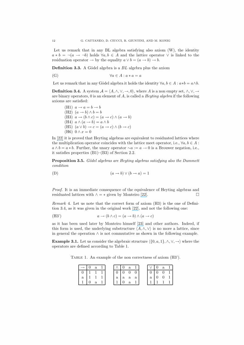
Definition 3.3. A Godel algebra is a BL algebra plus the axiom

(G) ∀a ∈ A : a ∗ a = a

Let us remark that in any Godel algebra it holds the identity ∀a, b ∈ A : a∗b = a∧b.

Definition 3.4. A system A = 〈A,∧,∨,→, 0〉, where A is a non empty set, ∧,∨,→are binary operators, 0 is an element of A, is called a Heyting algebra if the followingaxioms are satisfied:

(H1) a→ a = b→ b(H2) (a→ b) ∧ b = b(H3) a→ (b ∧ c) = (a→ c) ∧ (a→ b)(H4) a ∧ (a→ b) = a ∧ b(H5) (a ∨ b)→ c = (a→ c) ∧ (b→ c)(H6) 0 ∧ x = 0

In [22] it is proved that Heyting algebras are equivalent to residuated lattices wherethe multiplication operator coincides with the lattice meet operator, i.e., ∀a, b ∈ A :a ∧ b = a ∗ b. Further, the unary operator ∼a := a→ 0 is a Brouwer negation, i.e.,it satisfies properties (B1)–(B3) of Section 2.2.

Proposition 3.5. Godel algebras are Heyting algebras satisfying also the Dummettcondition

(D) (a→ b) ∨ (b→ a) = 1

Proof. It is an immediate consequence of the equivalence of Heyting algebras andresiduated lattices with ∧ = ∗ given by Monteiro [22]. �

Remark 4. Let us note that the correct form of axiom (H3) is the one of Defini-tion 3.4, as it was given in the original work [22], and not the following one:

(H3’) a→ (b ∧ c) = (a→ b) ∧ (a→ c)

as it has been used later by Monteiro himself [23] and other authors. Indeed, ifthis form is used, the underlying substructure 〈A,∧,∨〉 is no more a lattice, sincein general the operation ∧ is not commutative as shown in the following example.

Example 3.1. Let us consider the algebraic structure 〈{0, a, 1},∧,∨,→〉 where theoperators are defined according to Table 1.

Table 1. An example of the non correctness of axiom (H3’).

→ 0 a 10 1 1 1a 1 1 11 0 a 1

∧ 0 a 10 0 0 0a a a a1 0 a 1

∨ 0 a 10 0 0 1a 0 0 11 1 1 1

HEYTING WAJSBERG ALGEBRAS 13

Clearly, this structure satisfies all axioms (H1),(H2),(H3’), (H4), (H5) and (H6).However, the operators ∧ and ∨ do not define a lattice. For instance, the commu-tative property of ∧ is not satisfied, since a∧ 0 6= 0∧ a and ∨ is not an idempotentoperator, since a ∨ a = 0.

Definition 3.5. A system A = 〈A,∧,∨,→, ¬〉 is a symmetric Heyting algebra if itsatisfies (H1)–(H5) and ¬ is a de Morgan negation, i.e., it satisfies properties (K1)and (K2). Trivially, any symmetric Heyting algebra is a Heyting algebra oncedefined 0 := ¬(a→ a).

We can summarize the dependencies among these structures with the followingdiagram.

BL

vvnnnnnnnnnnnnn

))TTTTTTTTTTTTTTTTT

BL+(W) = Wajsberg Godel = BL+(G) = Heyting+(D)

3.1.1. BL lattice structure.

Proposition 3.6. Let 〈A,∧,∨, ∗,→, 0, 1〉 be a BL algebra. Then, once defined∼a := a → 0, the underlying lattice structure 〈A,∧,∨,∼, 0〉 is a pre–Brouwer deMorgan lattice.

Proof. We have to show that the following properties hold:

(B1) a ∧ ∼∼a = a;(B2b) ∼a ∨∼b = ∼(a ∧ b).

(B1). Setting b = 0 in axiom (b) we have ∼a ∗ a = 0. Setting a = ∼b in axiom(a), we have (∼b → (b ∗ ∼b)) ∧ b = b. Putting these two results together, we havea ∧ ∼∼a = a.(B2b). We prove that it holds in all linearly order BL algebras, then by Proposition3.3 it holds in any BL algebra. Let us suppose that a ≤ b. Then, we have ∼(a∧b) =∼a and on the other side ∼b ≤ ∼a by Proposition 3.1. Thus, ∼a ∨ ∼b = ∼a =∼(a ∧ b). �

The underlying structure is not a Brouwer lattice, because, in general, a BLalgebra does not satisfy the noncontradiction law ∀a : a ∧ ∼a = 0, as can be seenin the following counterexample.

Example 3.2. Let us consider the BL algebra, with support {0, a, b, 1} and oper-ators defined in Table 2.

Table 2. An example of {0, a, b, 1} BL algebra with ∗, → opera-tors and derived negation ∼ .

∗ 0 a b 10 0 0 0 0a 0 0 a ab 0 a b b1 0 a b 1

→ 0 a b 10 1 1 1 1a a 1 1 1b 0 a 1 11 0 a b 1

x ∼x0 1a ab 01 0

In figure 3, it is drawn the Hasse diagram of the underlying lattice structure.

14 G. CATTANEO, D. CIUCCI, R. GIUNTINI, AND M. KONIG

•1 = ∼0

• b

• a = ∼a

•

∼1 = 0 = ∼b

Figure 3. Hasse diagram of the lattice structure underlying theBL algebra of Table 2.

In this structure we have that a ∧∼a = a. So, ∼ is not a Brouwer negation andfurthermore it is not a de Morgan negation, since ∼∼b = 1 6= b.

Further, we have that in all BL algebras the Kleene condition is satisfied by the∼negation.

Proposition 3.7. Let 〈A,∧,∨, ∗,→, 0, 1〉 be a BL algebra. Then, for all a, b ∈ Athe condition

(K3) a ∧∼a ≤ b ∨∼b

holds.

Proof. We prove that (K3) holds in all linearly order BL algebras. Then, by Propo-sition 3.3, (K3) holds in any BL algebra. Let us suppose that a ≤ b, then, trivially,a ∧ ∼a ≤ a ≤ b ≤ b ∨ ∼b. On the other hand, if b ≤ a then by Proposition 3.1, wehave ∼a ≤ ∼b and finally, a ∧ ∼a ≤ ∼a ≤ ∼b ≤ b ∨ ∼b. �

3.2. Strict Basic Logic algebras. Let us consider BL algebras based on the unitinterval [0, 1] where ∗ is a triangular norm without non–trivial zero divisors [21],i.e., verifying:

∀a, b ∈ [0, 1] : x ∗ y = 0 iff a = 0 or b = 0.

So, the Godel algebra 〈[0, 1],∧,∨,→G, 0, 1〉 is an example of this kind of structure,whereas the Wajsberg algebra 〈[0, 1],→L, ¬, 1〉 is not. Following [16], a new axiomcan be introduced in BL algebras in order to obtain as models exactly these kindof structures.

Definition 3.6. A structure A = 〈A,∧,∨, ∗,→, 0, 1〉 is a Strict Basic Logic (SBL)algebra if it is a BL algebra and satisfies the further axiom

(a ∗ b)→ 0 = (a→ 0) ∨ (b→ 0)

Proposition 3.8. [16]. Let A be a Godel algebra then A is a SBL algebra.

Proposition 3.9. [16]. Let φ and ψ be well-defined terms, in the traditional way,on the language of SBL algebra. An equation φ = ψ is satisfied in all linearlyordered SBL algebras iff it is satisfied in all SBL algebras.

HEYTING WAJSBERG ALGEBRAS 15

3.2.1. SBL lattice structure.

Lemma 3.1. Let A be a SBL algebra and define ∼a := a→ 0. Then, for all a ∈ A,the condition

a ∧ ∼a = 0

holds.

Proof. By Definition 3.6 and de Morgan properties ∼(a ∗ b) = ∼a ∨ ∼b = ∼(a ∧ b)and by BL axiom (f) ∼(a ∗ b) = ∼(a ∗ (a → b)). Now, by the property x ∗ ∼x = 0we have

0 = [a ∗ (a→ b)] ∗ ∼[a ∗ (a→ b)] = [a ∗ (a→ b)] ∗ ∼(a ∗ b).

Finally, setting b = ∼a, we have the thesis. �

Proposition 3.10. Let 〈A,∧,∨, ∗,→, 0, 1〉 be a SBL algebra. Once defined ∼a :=a→ 0, the structure 〈A,∧,∨,∼, 0〉 is a de Morgan Brouwer lattice.

Proof. Since any SBL algebra is a BL algebra and hence a pre–Brouwer lattice, wehave only to prove that a ∧ ∼a = 0 which is just Lemma 3.1. �

3.3. SBL¬ algebras. Finally, a new unary operator is added to SBL algebras.The axioms characterizing this new operator are developed in order to obtain a deMorgan negation i.e., a negation satisfying the double negation law, “∀a : ¬¬a = a”and the contraposition law “∀a, b : ¬a ≤ ¬b implies b ≤ a”; and in order to definea unary operator ν as the algebraic counterpart of the Baaz operator ∆ [1].

Definition 3.7. A system A = 〈A,∧,∨, ∗,→,¬, 0, 1〉 is a SBL¬ algebra if

(1) 〈A,∧,∨, ∗,→, 0, 1〉 is a SBL algebra(2) ¬ is a unary operator such that, once defined ∼a = a→ 0 and ν(a) = ∼¬a,

the following are satisfied(SBL¬1) ¬¬a = a(SBL¬2) ∼a ≤ ¬a(SBL¬3) ν(a→ b) = ν(¬b→ ¬a)(SBL¬4) ν(a) ∨ ν(¬a) = 1(SBL¬5) ν(a ∨ b) ≤ ν(a) ∨ ν(b)(SBL¬6) ν(a) ∗ (ν(a→ b)) ≤ ν(b)

Proposition 3.11. [16]. Let φ and ψ be well-defined terms, in the traditional way,on the language of SBL¬ algebra. An equation φ = ψ is satisfied in all linearlyordered SBL¬ algebras iff it is satisfied in all SBL¬ algebras.

3.3.1. SBL¬ lattice structure.

Proposition 3.12. Let 〈A,∧,∨, ∗,→,¬, 0, 1〉 be a SBL¬ algebra. Then, once de-fined ∼a := a→ 0, the structure 〈A,∧,∨,¬,∼, 0〉 is BZdM lattice.

Proof. Since any SBL¬ algebra is a SBL algebra and hence a Brouwer de Morganlattice, we have only to prove that

(K1) ¬¬a = a(K2) ¬(a ∨ b) = ¬a ∧ ¬b(K3) a ∧ ¬a ≤ b ∨ ¬b(in) ¬∼a = ∼∼a

16 G. CATTANEO, D. CIUCCI, R. GIUNTINI, AND M. KONIG

(K1) It is an axiom of SBL¬ algebras.(K2) It has been proved in [16].(K3) Similar to Proposition 3.7.(in) By ∼a ≤ ¬a, we get ∼a = ∼a ∧ ¬a, and applying this to ν(a): ∼ν(a) =∼ν(a) ∧ ¬ν(a). By axioms (a) and (b), we have ¬ν(a) = ¬ν(a) ∧ [ν(a)→ (¬ν(a) ∗ν(a))] = ¬ν(a) ∧ ∼ν(a). So, we have that ∼ν(a) = ¬ν(a), which, once applied to¬a, gives the thesis. �

4. HW algebras

At the top level of our hierarchy, we introduce and study the new structure ofHeyting Wajsberg (HW) algebra [5, 7]. Its originality consists in the presence oftwo implication connectives as primitive operators.

Definition 4.1. A system A = 〈A,→L,→G, 0〉 is a Heyting Wajsberg (HW ) alge-bra if A is a non empty set, 0 ∈ A and →L,→G are binary operators, such that,once defined

1 := ¬0(2a)

¬a := a→L 0(2b)

∼a := a→G 0(2c)

a ∧ b := ¬((¬a→L ¬b)→L ¬b)(2d)

a ∨ b := (a→L b)→L b(2e)

the following are satisfied:

(HW1) a→G a = 1(HW2) a→G (b ∧ c) = (a→G c) ∧ (a→G b)(HW3) a ∧ (a→G b) = a ∧ b(HW4) (a ∨ b)→G c = (a→G c) ∧ (b→G c)(HW5) 1→L a = a(HW6) a→L (b→L c) = ¬(a→L c)→L ¬b(HW7) ¬∼a→L ∼∼a = 1(HW8) (a→G b)→L (a→L b) = 1

Lemma 4.1. In any HW algebra the following properties hold

(L1) a→L a = 1(L2) a→L b = ¬b→L ¬a(L3) ¬¬a = a(L4) a ∧ 1 = a; 1 ∧ a = a(L5) 1→G c = c(L6) a ∧ b = b ∧ a

Proof. (L1) Setting b = a in (HW8) and using (HW1), we get 1→L (a→L

a) = 1. Now, by (HW5) we have the thesis.(L2) Setting a = 1 in (HW6), we have 1→L (b→L c) = ¬(1→L c)→L ¬b,

then by (HW5) we derive the thesis.(L3) First, by definition of ¬ and (HW5), we can derive that ¬1 = 0. Now,

applying (L2) to (HW5), we get ¬a →L ¬1 = a. Finally, by ¬1 = 0and definition of ¬, we get ¬¬a = a.

HEYTING WAJSBERG ALGEBRAS 17

(L4) By ∧ definition:

a ∧ 1 = ¬((¬a→L ¬1)→L ¬1) (L2), (L3)

= ¬(1→L ¬(1→L a)) (HW5)

= ¬(1→L ¬a) (HW5), (L3)

= ¬¬a = a

Similarly, we get 1 ∧ a = a.(L5) Setting a = b = 1 in (HW2), we get 1→G (1∧ c) = (1→G c)∧ (1→G

1). Then, by (HW1) and (L4) we have the thesis.(L6) Simply by setting a = 1 in (HW2) and using (L5).

�

Proposition 4.1. Let A be a HW algebra. Then, the following equations aremutually equivalent:

a→L b = 1(3a)

a→G b = 1(3b)

a ∧ b = a(3c)

Proof. a→L b = 1 implies a ∧ b = a. By definition of ∧:

a ∧ b = ¬[(¬b→L ¬a)→L ¬a) (L2), (L3)

= ¬[a→L ¬(a→L b)] Hypothesis

= ¬(a→L ¬1) (L2), (HW5), (L3)

= ¬¬a = a

b ∧ a = a implies a→G b = 1. Setting c = a in axiom (HW2) we get:

a→G (b ∧ a) = (a→G b) ∧ (a→G a) Hypothesis, (HW1)

a→G a = (a→G b) ∧ 1 (HW1), (L4)

1 = a→G b

a →G b = 1 implies a →L b = 1. Using (HW8) and hypothesis, one has1→L (a→L b) = 1. Then by axiom (HW5), a→L b = 1.

�

Proposition 4.2. Let A be a HW algebra. The binary operator ≤ defined as

a ≤ b iff a→L b = 1 (equivalently, iff a→G b = 1 iff a ∧ b = a)

is a partial order on A.

Proof. a ≤ a is property (L1).Let us suppose that a ≤ b and b ≤ a. By (HW3) and a→G b = 1 we get a = a ∧ b.Dually, by (HW3) and b →G a = 1 we have b = b ∧ a and by (L6) we have thethesis.Finally, let us suppose that a ≤ b and b ≤ c. By (HW2) and (L4), we obtain1 = (a→G c), that is a ≤ c. �

The following result is now quite trivial.

18 G. CATTANEO, D. CIUCCI, R. GIUNTINI, AND M. KONIG

Proposition 4.3. The concrete structure 〈[0, 1],→L,→G, 0〉 based on the real unitinterval, where the operators →L and →G are the ones introduced in equations (1a)and (1b), satisfies HW axioms. As its name suggests, an HW algebra is a pastingof a Heyting and a Wajsberg algebra as stated in the following propositions.

Proposition 4.4. Let A be a HW algebra. Then, by defining ∧ and ∨ as in Defi-nition 4.1, we have that 〈A,→G,∧,∨,¬〉 is a symmetric Heyting algebra accordingto Definition 3.4.

Proof. Axioms (H1), (H3), (H4) and (H5) are axioms (HW1)–(HW4). We prove(H2). By definition of ∧ and setting b = 1 in (HW4) we have:

1→G c = ¬{[¬(a→G c)→L ¬(1→G c)]→L ¬(1→G c)}

By (L5) and ∧ definition we obtain c = (a→G c) ∧ c, i.e., (H2).(K1) is property (L3). (K2) follows from ∧,∨ definitions and (K1). �

Proposition 4.5. Let A be a HW algebra. Then 〈A,→L,¬, 1〉 is a Wajsberg algebraaccording to Definition 3.2.

Proof. Axiom (W1) is axiom (HW5). Axiom (W2) can be derived by the latticeproperty b ∧ a ≤ b ∨ c and Proposition 4.1 as follows:

1 = b ∧ a→L b ∨ c Def. ∧,∨

= ¬((¬b→L ¬a)→L ¬a)→L ((b→L c)→L c) (L2)

= ¬((a→L b)→L ¬a)→L ((b→L c)→L c) (HW6)

= (a→L b)→L ¬(((b→L c)→L c)→L ¬a) (HW6)

= (a→L b)→L ((b→L c)→L (a→L c))

By definition of ∨, axiom (W3) is equivalent to a ∨ b = b ∨ a which holds in anylattice (and hence in any Heyting algebra). Finally, axiom (W4) can be derived byproperty (L2). �

When considering the underlying lattice structure of HW algebras, the followingresult can be proved.

Proposition 4.6. Let A be a HW algebra. Then, once defined ∧, ∨, ∼, ¬ and 1as in Definition 4.1, the structure 〈A,∧,∨,¬, ∼, 0, 1〉 is a BZdM lattice.

Proof. Due to Theorems 4.4 and 4.5, the only properties that still need a proof are

¬ ∼a = ∼∼a(in)

∼ (a ∧ b) = ∼a ∨∼b(dM)

The first one follows from (HW7) and (HW8). Indeed, by (HW7) we have ¬∼a ≤∼∼a. By (HW8) with b = 0 we get∼a ≤ ¬a which applied to∼a gives∼∼a ≤ ¬∼aand so (in) is verified.

Let us prove the second one. As proved in [25], in a pseudo complemented lattice[2, p. 125] and hence, in any Heyting algebra, the Stone condition

(S) ∼a ∨ ∼∼a = 1

implies the de Morgan property (dM). So, it is sufficient to prove that (S) holdsin any HW algebra. Let a ∈ A and define y = ∼a. So, by (in) we get ∼y = ¬y.Using the non contradiction law for the Brouwer negation y ∧ ∼y = 0 (it holds inany pseudo complemented lattice [27, p. 60] hence in any Heyting algebra [22] and

HEYTING WAJSBERG ALGEBRAS 19

by Theorem 4.4 in any HW algebra), we derive y ∧ ¬y = 0 and then y ∨ ¬y = 1.Finally, we get y ∨ ∼y = 1, that is ∼a ∨ ∼∼a = 1. �

Hence, as we did in BZ lattices (see Definition 2.4), also in any HW algebra A itis possible to define the anti–intuitionistic negation as ♭(a) := ¬∼ ¬a. Further, alsothe modal–like operators of necessity ν(a) := ∼¬a and possibility µ(a) := ¬∼asatisfy all the properties of Section 2.3.1. Finally, in any HW algebra it is possibleto induce an abstract approximation space in the sense of Definition 2.5.

Remark 5. It is well known that in any lattice it holds the duality principle [27], i.e.,(∧,∨) and (0, 1) are pair of dual operators: by replacing an operator with the dualone in a true statement, we again obtain a true statement. Monteiro [23] provedthat a duality principle holds also for symmetric Heyting algebras, i.e., Heytingalgebras with a de Morgan negation ¬. This result can be extended in a naturalway to HW algebras defining the dual operators of the Godel and Lukasiewiczimplications respectively as a←G b := ¬(¬a→G ¬b) and a←L b := ¬(¬a→L ¬b).

4.1. Monteiro implication. The two primitive implications, Lukasiewicz andGodel, are not the only one definable in HW algebras. Here we focus our attentionon a third kind of implication, called “faible” in Monteiro [23]. This operator isstrictly linked to modalities and to the anti–intuitionistic negation.

Definition 4.2. For any pair a, b of elements of a HW algebra the Monteiro im-plication is defined as:

a→M b := µ(¬a) ∨ b

It can be shown that the following hold.

Proposition 4.7. In any HW algebra the Monteiro implication satisfies the fol-lowing properties:

(M1) a→M a = 1(M2) a→M (b→M a) = 1(M3) a→M (b→M c) = (a→M b)→M (a→M c)(M4) ((a→M b)→M a)→M a = 1(M5) 1→M a = a(M6) a→M 0 = ♭a

Proof. These properties hold in all Heyting algebras with a Kleene negation ¬satisfying also the Stone condition (S) of ∼ [23], hence they are valid also in HWalgebras. �

We remark that, as stated in (M6), the Monteiro implication permits to introduceindependently the anti-intuitionistic negation.

Since we are greatly interested in the unit interval, it is natural to considerhow behaves this kind of implication in [0, 1] and if it can be can defined as theresiduation of a t–norm. The following proposition is an answer to these questions.

Proposition 4.8. Let us consider the Monteiro implication on the unit interval[0, 1]. It does not exist a t–norm t such that →M is the residuation of t , i.e., suchthat for all a, b ∈ [0, 1]

a→M b = sup{c ∈ [0, 1] : atc ≤ b}

20 G. CATTANEO, D. CIUCCI, R. GIUNTINI, AND M. KONIG

Proof. Once considered on the unit interval, the Monteiro implication reduces to

a→M b =

{

b if a = 1

1 otherwise

Now, suppose that there exists a t–norm t generating →M . Then, for all a 6= 1and for all b it should hold that at1 ≤ b. But if t is a t–norm then it musthold at1 = a, and consequently a ≤ b, which, clearly, is not satisfied by all pairs〈a, b〉 ∈ [0, 1)× [0, 1]. �

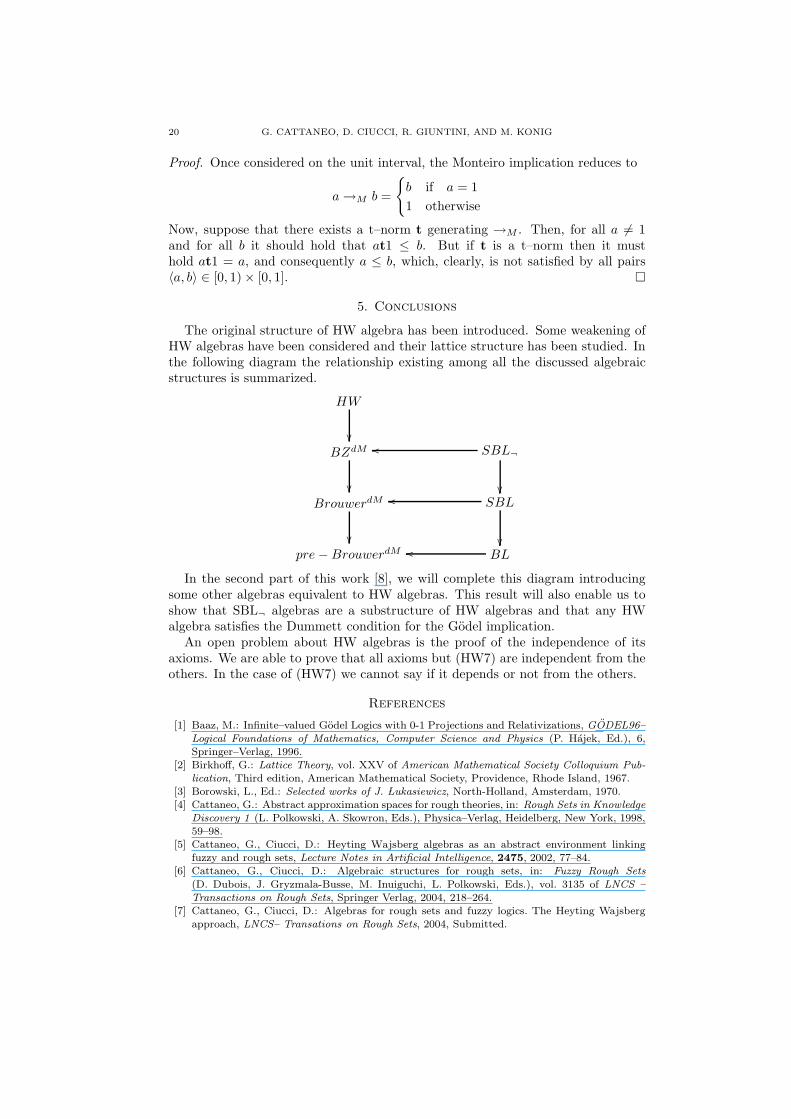
5. Conclusions

The original structure of HW algebra has been introduced. Some weakening ofHW algebras have been considered and their lattice structure has been studied. Inthe following diagram the relationship existing among all the discussed algebraicstructures is summarized.

HW

��

BZdM

��

SBL¬oo

��

BrouwerdM

��

SBLoo

��

pre−BrouwerdM BLoo

In the second part of this work [8], we will complete this diagram introducingsome other algebras equivalent to HW algebras. This result will also enable us toshow that SBL¬ algebras are a substructure of HW algebras and that any HWalgebra satisfies the Dummett condition for the Godel implication.

An open problem about HW algebras is the proof of the independence of itsaxioms. We are able to prove that all axioms but (HW7) are independent from theothers. In the case of (HW7) we cannot say if it depends or not from the others.

References

[1] Baaz, M.: Infinite–valued Godel Logics with 0-1 Projections and Relativizations, GODEL96–

Logical Foundations of Mathematics, Computer Science and Physics (P. Hajek, Ed.), 6,Springer–Verlag, 1996.

[2] Birkhoff, G.: Lattice Theory, vol. XXV of American Mathematical Society Colloquium Pub-

lication, Third edition, American Mathematical Society, Providence, Rhode Island, 1967.[3] Borowski, L., Ed.: Selected works of J. Lukasiewicz, North-Holland, Amsterdam, 1970.[4] Cattaneo, G.: Abstract approximation spaces for rough theories, in: Rough Sets in Knowledge

Discovery 1 (L. Polkowski, A. Skowron, Eds.), Physica–Verlag, Heidelberg, New York, 1998,59–98.

[5] Cattaneo, G., Ciucci, D.: Heyting Wajsberg algebras as an abstract environment linkingfuzzy and rough sets, Lecture Notes in Artificial Intelligence, 2475, 2002, 77–84.

[6] Cattaneo, G., Ciucci, D.: Algebraic structures for rough sets, in: Fuzzy Rough Sets

(D. Dubois, J. Gryzmala-Busse, M. Inuiguchi, L. Polkowski, Eds.), vol. 3135 of LNCS –

Transactions on Rough Sets, Springer Verlag, 2004, 218–264.[7] Cattaneo, G., Ciucci, D.: Algebras for rough sets and fuzzy logics. The Heyting Wajsberg

approach, LNCS– Transations on Rough Sets, 2004, Submitted.

HEYTING WAJSBERG ALGEBRAS 21

[8] Cattaneo, G., Ciucci, D., Giuntini, R., Konig, M.: Algebraic Structures Related to Many Val-ued Logical Systems. Part II: Equivalence Among some Widespread Structures, Fundamenta

Informaticae, 2004, Accepted.[9] Cattaneo, G., Dalla Chiara, M. L., Giuntini, R.: Some Algebraic Structures for Many-Valued

Logics, Tatra Mountains Mathematical Publication, 15, 1998, 173–196, Special Issue: Quan-tum Structures II, Dedicated to Gudrun Kalmbach.

[10] Cattaneo, G., Marino, G.: Brouwer-Zadeh posets and fuzzy set theory, Proceedings of the

1st Napoli Meeting on Mathematics of Fuzzy Systems (A. Di Nola, A. Ventre, Eds.), Napoli,June 1984.

[11] Cattaneo, G., Nistico, G.: Brouwer-Zadeh Posets and Three valued Lukasiewicz posets, Fuzzy

Sets Syst., 33, 1989, 165–190.[12] Chellas, B. F.: Modal Logic, An Introduction, Cambridge University Press, Cambridge, MA,

1988.[13] Cignoli, R.: Injective de Morgan and Kleene Algebras, Proceedings of the American Mathe-

matical Society, 47(2), 1975, 269–278.[14] Dunn, J. M.: Relevance logic and entailment, in: Handbook of Philosophical Logic (D. Gab-

bay, F. Guenther, Eds.), vol. 3, Kluwer, 1986, 117–224.[15] Dunn, J. M., Hardegree, G. M.: Algebraic Methods in Philosophical Logic, vol. 41 of Oxford

Logic Guides, Clarendon Press, 2001.

[16] Esteva, F., Godo, L., Hajek, P., Navara, M.: Residuated Fuzzy logics with an involutivenegation, Archive for Mathematical Logic, 39, 2000, 103–124.

[17] Esteva, F., Godo, L., Montagna, F.: The LΠ and LΠ 1

2logics: two complete fuzzy systems

joining Lukasiewicz and Product Logics, Archive for Mathematical Logic, 40, 2001, 39–67.[18] Goldblatt, R.: Mathematical modal logic: A view of its evolution, J. Applied Logic, 1, 2003,

309–392.[19] Hajek, P.: Metamathematics of Fuzzy Logic, Kluwer, Dordrecht, 1998.[20] Kalman, J.: Lattices with involution, Transactions of the American Mathematica Society,

87(2), 1958, 485–491.[21] Klement, E. P., Mesiar, R., Pap, E.: Triangular Norms, Kluwer Academic, Dordrecht, 2000.[22] Monteiro, A.: Axiomes Independants pour les Algebres de Brouwer, Revista de la Union

matematica Argentina y de la Asociacion Fisica Argentina, 17, 1955, 149–160.[23] Monteiro, A.: Sur Les Algebres de Heyting symetriques, Portugaliae Mathematica, 39, 1980,

1–237.[24] Monteiro, A.: Unpublished papers, I, vol. 40 of Notas de Logica Matematica, Universidad

Nacional del Sur, Bahia Blanca, 1996.[25] Monteiro, A., Monteiro, L.: Algebres de Stone libres, in: Unpublished papers, I [24].[26] Rasiowa, H.: An Algebraic Approach to Non–Classical Logics, North Holland, Amsterdam,

1974.[27] Rasiowa, H., Sikorski, R.: The Mathematics of Metamathematics, vol. 41 of Monografie

Matematyczne, Third edition, Polish Scientific Publishers, Warszawa, 1970.[28] Rescher, N.: Many-valued logic, Mc Graw-hill, New York, 1969.[29] Surma, S.: Logical Works, Polish Academy of Sciences, Wroclaw, 1977.[30] Turunen, E.: Mathematics Behind Fuzzy Logic, Physica–Verlag, Heidelberg, 1999.[31] Wajsberg, M.: Aksjomatyzacja trowartosciowego rachunkuzdan [Axiomatization of the three-

valued propositional calculus], Comptes Rendus des Seances de la Societe des Sciences et des

Lettres de Varsovie, 24, 1931, 126–148, English Translation in [29].[32] Wajsberg, M.: Beitrage zum Metaaussagenkalkul I, Monashefte fur Mathematik un Physik,

42, 1935, 221–242, English Translation in [29].[33] Ward, M., Dilworth, R.: Residuated Lattices, Transactions of the American Mathematical

Society, 45(3), 1939, 335–354.

Dipartimento di Informatica, Sistemistica e Comunicazione, Universita di Milano–Bicocca, Via Bicocca degli Arcimboldi 8, I–20126 Milano (Italy)

E-mail address: {cattang,ciucci}@disco.unimib.it

Dipartimento di Scienze Pedagogiche e Filosofiche, Universita di Cagliari, Via IsMirrionis 1, 09123 Cagliari (Italia)

E-mail address: giuntini@unica.it, martinvk@iol.it