Citation: Fitz, A.C.; Gómez Trillos,

J.C.; Sill Torres, F. AIS-Based

Estimation of Hydrogen Demand

and Self-Sufficient Fuel Supply

Systems for RoPax Ferries. Energies

2022, 15, 3482. https://doi.org/

10.3390/en15103482

Academic Editors: Dheeraj

Bharadwaj Gosala and Cody

Michael Allen

Received: 30 March 2022

Accepted: 6 May 2022

Published: 10 May 2022

Publisher’s Note: MDPI stays neutral

with regard to jurisdictional claims in

published maps and institutional affil-

iations.

Copyright: © 2022 by the authors.

Licensee MDPI, Basel, Switzerland.

This article is an open access article

distributed under the terms and

conditions of the Creative Commons

Attribution (CC BY) license (https://

creativecommons.org/licenses/by/

4.0/).

energies

Article

AIS-Based Estimation of Hydrogen Demand and Self-SufficientFuel Supply Systems for RoPax FerriesAnnika Christine Fitz 1,* , Juan Camilo Gómez Trillos 2 and Frank Sill Torres 3

1 German Aerospace Centre, Institute of Maritime Energy Systems, Max-Planck-Straße 2,21502 Geesthacht, Germany

2 German Aerospace Centre, Institute of Networked Energy Systems, Carl-von-Ossietzky-Straße 15,26129 Oldenburg, Germany; juan.gomeztrillos@dlr.de

3 German Aerospace Centre, Institute for the Protection of Maritime Infrastructures, Fischkai 1,27572 Bremerhaven, Germany; frank.silltorres@dlr.de

* Correspondence: annika.fitz@dlr.de; Tel.: +49-4152-84881-18

Abstract: The International Maritime Organization (IMO) established new strategies that could leadto a significant reduction in the carbon footprint of the shipping sector to address global warming.A major factor in achieving this goal is transitioning to renewable fuels. This implies a challenge,as not only ship-innovative solutions but also a complete low-carbon fuel supply chain must beimplemented. This work provides a method enabling the exploration of the potential of low-carbonfuel technologies for specific shipping routes up to larger sea regions. Several aspects includingvessel sizes, impact of weather and shipping routes, emissions savings and costs are considered. Thelocal energy use is determined with proven bottom-up prediction methods based on ship positioningdata from the Automatic Identification System (AIS) in combination with weather and ship technicaldata. This methodology was extended by an approach to the generation of a basic low-carbon fuelsystem topology that enables the consideration of local demand profiles. The applicability of theproposed approach is discussed at hand via a case study on Roll-on/Roll-off passenger and cargo(RoPax) ferries transitioning from conventional fuels to a compressed hydrogen fuel system. Theresults indicate a potential reduction in emissions by up to 95% and possible system sizes and costs.

Keywords: emissions reduction; alternative marine fuels; hydrogen technologies; ship energy useestimation

1. Introduction

The European Commission and the International Maritime Organization (IMO) adoptedsevere reduction targets in carbon dioxide (CO2) emissions, which is a major greenhousegas (GHG), for the marine sector [1,2]. Further substances such as nitrous oxides (NOx),sulfuric oxides (SOx) and particular matter (PM) are typical pollutants from diesel enginecombustion [3]. They are associated with hazardous effects on the environment and humanhealth [4].

Hence, the marine sector is facing the need to transition to cleaner low-carbon fuels,such as hydrogen, ammonia or methanol from renewable energy sources. While the targetsare clear, the pathways to get there remain vague. Without reliable supply chains andsystems, ship owners hesitate to order shipyards to construct ships with novel propulsionand fuel systems. Fuel producers and infrastructure providers, on the other hand, willnot invest without predictable demand [5]. Pilot projects involving all stakeholders arerequired to demonstrate the feasibility of new fuel systems and attract further marketplayers to invest.

Roll-on/roll-off passenger and cargo (RoPax) ferries can be identified as an attractivecandidate for pilot projects. These types of ships carry passengers, cars and trucks mostlybetween two and sometimes among several different ports. Their stable location and

Energies 2022, 15, 3482. https://doi.org/10.3390/en15103482 https://www.mdpi.com/journal/energies

Energies 2022, 15, 3482 2 of 23

predictable energy demand reduce the uncertainty of integrating novel fuel systems. Inthe European market in 2019, 1396 operating RoPax vessels were registered. Ship sizesrange from 30–240 m, from small river-crossing vessels up to super-ferries connectinginternational trading ports [6]. For 363 ships with a gross tonnage (gt) larger than 5000 t, atotal fuel consumption of 4.4 Mt in 2019 was reported [7]. This accounts for 9% of the totalmarine fuel mass consumed in the EU [8].

The processing of ship positioning data from a ship’s automatic identification system(AIS) is a common approach to estimate fuel consumption and related emissions and hasbeen applied in various studies. The SHIP-DESMO model by Kristensen et al. estimates theenergy use and ship emissions at different ship speeds based on a ship resistance model byHarvald (1983); missing ship technical data can be supplemented with statistical data [9].In conjunction with AIS data, the model was used in an emissions inventory of the ArcticSea by Winther et al. [10]. The STEAM model by Jalkanen et al. is based on ship resistanceprediction methods presented by Hollenbach in 1998 and incorporates added resistance bysea conditions [11]. It was applied for emission inventories in the Baltic Sea in 2014 [12] andin European sea areas in 2016 [13]. On the largest scale, one can remark on studies carriedout by the IMO on international waters, employing the propeller curve with constant valuesfor weather effects and fouling in their Greenhouse Gas Studies from the years 2014 [14,15]and 2020 [15]. All listed methods are limited to analysis of the existing state and are notable to explore the potential of alternative fueling solutions.

General cost evaluations on utilizing hydrogen as an alternative energy carrier wereperformed by the Hydrogen Council, estimating the competitiveness in USD/km of trans-portation for RoPax ferries in the lower MW power range [16]. While this report providesa general indication of competitiveness, route and location-specific aspects, such as thespecific operational and energy use profile or site-specific weather conditions, were notconsidered. Aarskog et al. presented an energy and cost analysis of a hydrogen-drivenhigh-speed passenger ferry in Norway [17]. An AIS-based energy use profile and costcalculations were aligned with the installed equipment of the specific ship.

In this paper we provide a scheme that is able to consider ship and site-specific aspectsand is also transferable to various locations and shipping routes. AIS-based methods areutilized to generate localized energy use profiles for RoPax ferries as an existing-stateanalysis incorporating the ship propeller curve model and weather conditions. The existingstate of energy use is extended with an outlook on possible future setups utilizing low-carbon technology. A feasible low-carbon fuel system setup is generated based on thelocalized energy use profile. This allows for exploring the possibilities and benefits oftransitioning to low-carbon technologies in terms of energy efficiency, emissions savingsand system costs on a system component level. The explored scenarios were chosen toconsider the whole supply chain, from renewable production to storage, distribution andend use, by estimating appropriate sizes of each system component. The generated fuelsystem scenario for a specific location may then support transparency and understandingin developing local synergetic systems.

This paper focuses on the use of compressed hydrogen systems. The method is genericand can be extended to other energy carriers. Figure 1 depicts the main components of amarine hydrogen fuel system that employs renewable resources. Here, a wind farm gener-ates renewable energy, which feeds an electrolyser that produces hydrogen. The hydrogenis stored in an intermediate storage system and transported to the fuel station. At the fuelstation, conditioned hydrogen is supplied to the RoPax vessels. The ships are equippedwith a fuel cell propulsion system, generating electricity to supply an electric motor. As atypical setup, the fuel cell is combined with a battery in a hybrid configuration [18]. Theoption of landside charging of these ship batteries, likewise from the renewable energysource, is modeled.

Energies 2022, 15, 3482 3 of 23Energies 2022, 15, x FOR PEER REVIEW 3 of 23

Figure 1. Marine hydrogen fuel system (Source: Created by author using Flaticon.com (accessed on 31 March 2021)).

The rest of this work is structured as follows. Section 2 presents the relevant methods of AIS energy use estimation as well as the state of technology for hydrogen fuel system components. In Section 3, the implementation of energy use estimation is presented, as well as the developed methodology for generating a low-carbon fuel system based on the localized energy use profile. Section 4 discusses a case study, and Section 5 concludes this work.

2. Preliminaries This section describes the principles of AIS-based energy use estimation and the cur-

rently available technology relevant for marine hydrogen fuel systems.

2.1. Energy Use Prediction The energy usage of ships can be determined by two different approaches, namely

top-down and bottom-up methods. While top-down methods utilize measurements of consumed fuel quantities in retrospect to derive the energy use, bottom-up methods em-ploy ship activity data, such as ship speed and weather conditions [18]. One advanced and equally common approach for tracking ship activity is recording and processing sig-nals of the Automatic Identification System (AIS). AIS is a ship positioning data system, originally developed for collision prevention and made mandatory for passenger ships by the IMO [19]. Frequently exchanged messages among ships, terrestrial antennas and sat-ellites contain information concerning the ship’s speed, heading, draught and in some cases also further technical data such as ship dimensions, loaded cargo and destination [20].

The required propulsive power produced by the main engines 𝑃 can be estimated as a cubic function of ship speed 𝑣, commonly known as the propeller curve. The power is usually referenced to a power reference 𝑃 at a reference speed 𝑣 . It can be ex-tended by considering the ship’s ratio of actual to reference draught 𝑇/𝑇 to the power of ⅔ as shown in Equation (1) [21].

𝑃 = 𝑃 ∗ 𝑇𝑇 ∗ 𝑣𝑣 (1)

In many cases, the installed main engine power 𝑃 , will exceed 𝑃 due to safety or market availability reasons. Hence, it should be corrected with the downscaling factor 𝜀 as applied by Jalkanen to obtain 𝑃 , as depicted in Equation (2) [22]. 𝑃 = 𝑃 , ∗ 𝜀 (2)

The reference power 𝑃 applies in reference conditions, i.e., a steady-state move-ment in calm water, without wind, with a clean ship hull and great water depth [21]. In

Figure 1. Marine hydrogen fuel system (Source: Created by author using Flaticon.com (accessed on31 March 2021)).

The rest of this work is structured as follows. Section 2 presents the relevant methodsof AIS energy use estimation as well as the state of technology for hydrogen fuel systemcomponents. In Section 3, the implementation of energy use estimation is presented, aswell as the developed methodology for generating a low-carbon fuel system based on thelocalized energy use profile. Section 4 discusses a case study, and Section 5 concludesthis work.

2. Preliminaries

This section describes the principles of AIS-based energy use estimation and thecurrently available technology relevant for marine hydrogen fuel systems.

2.1. Energy Use Prediction

The energy usage of ships can be determined by two different approaches, namelytop-down and bottom-up methods. While top-down methods utilize measurements ofconsumed fuel quantities in retrospect to derive the energy use, bottom-up methodsemploy ship activity data, such as ship speed and weather conditions [18]. One advancedand equally common approach for tracking ship activity is recording and processingsignals of the Automatic Identification System (AIS). AIS is a ship positioning data system,originally developed for collision prevention and made mandatory for passenger shipsby the IMO [19]. Frequently exchanged messages among ships, terrestrial antennas andsatellites contain information concerning the ship’s speed, heading, draught and in somecases also further technical data such as ship dimensions, loaded cargo and destination [20].

The required propulsive power produced by the main engines PME can be estimatedas a cubic function of ship speed v, commonly known as the propeller curve. The power isusually referenced to a power reference Pre f at a reference speed vre f . It can be extendedby considering the ship’s ratio of actual to reference draught T/Tre f to the power of 2⁄3 asshown in Equation (1) [21].

PME = Pre f ∗(

TTre f

) 23

∗(

vvre f

)3

(1)

In many cases, the installed main engine power PME,inst will exceed Pre f due to safetyor market availability reasons. Hence, it should be corrected with the downscaling factorεp as applied by Jalkanen to obtain Pre f , as depicted in Equation (2) [22].

Pre f = PME,inst ∗ εp (2)

The reference power Pre f applies in reference conditions, i.e., a steady-state movementin calm water, without wind, with a clean ship hull and great water depth [21]. In opera-tional, real sea conditions, hull fouling, shallow waters and steering can all lead to higher

Energies 2022, 15, 3482 4 of 23

resistance. The added resistance can be expressed by the speed penalty ∆v/v [23]. Thus,the required propulsive power P can be stated according to Equation (3):

PME = εP ∗ PME, inst ∗(

TTre f

) 23

∗

v ∗(

1 + ∆vv

)vre f

3

(3)

Next to the main engine delivering propulsive power, an auxiliary engine serves allfurther power needs PAE such as on-board electricity or bow and stern thrusters.

Installed auxiliary power PAE, inst can be estimated as a proportion of PME,inst and itsload factor in operation LFAE depending on the operating state (e.g., at berth, maneuvering,cruising), as shown by Equation (4).

PAE = PAE, inst ∗ LFAE (4)

This approach was utilized by the United States Environmental Protection Agency(EPA) in 2010 [18]. Other approaches use fixed power values per operating states, e.g., IMO2020 [15], or include the number of cabins for passenger ships, as in Jalkanen 2012 [11].

The total fuel consumption m f uel is summed over n AIS operating points, recorded invarying time intervals ∆t with the main engine power PME,n and auxiliary engine powerPAE,n at their instantaneous fuel oil consumptions SFOCME,n and SFOCAE,n within a timeinterval ∆t, as described in Equation (5).

m f uel =n

∑0(PME,n ∗ SFOCME,n + PAE,n ∗ SOFCAE,n) ∗ ∆t (5)

The specific fuel-oil consumption (SFOC) is the efficiency parameter of the main orauxiliary engine and depends on its type, model year, fuel type and exhaust aftertreatmentsystem. Base values tabulated by the IMO are utilized and referred to as SFOCB [15].Furthermore, SFOCB can be corrected to the load-specific fuel oil consumption SFOCL atdifferent engine load factors LF [15]. The correction formula is here shown as Equation (6):

SFOCL = SFOCB ∗(

0.455 ∗ LF2 − 0.71 ∗ LF + 1.28)

(6)

The mass of combustion emissions mp is calculated for the pollutants p (CO2, NOx, SOx,PM2.5) with Equation (5) and emission factors EF according to IMO GHG 2020 [15], em-ploying Equation (7).

mp = m f uel ∗ EFp (7)

2.2. Energy Supply with Hydrogen as Energy Carrier

Hydrogen is not an energy source per se but an energy carrier. Its supply chainconsists of an energy source used for the production of hydrogen molecules, hydrogenproduction equipment, storage, transport, a fuel station and finally the propulsive systemof the vessel, as shown in Figure 1. This section introduces different technology options forsuch a fuel sytem.

In order to reduce carbon emissions by utilizing hydrogen, the primary energy sourcemust be low-carbon, such as wind or solar power. In this particular case only, hydrogen isdenominated as ‘green hydrogen’ [24]. Most commonly, green hydrogen is produced byelectrolysis, the splitting of water molecules between two electrodes with the addition ofelectric energy [25], i.e.,

H2O H2 + 0.5 O2 ∆H = +285.8 kJ

mol(8)

Energies 2022, 15, 3482 5 of 23

Different types of electrolysers are distinguished by their electrolyte. The commerciallyavailable types are polymer exchange membrane (PEM) and Alkaline [25]. In their currentstate, both types of technology achieve similar system sizes and costs [26].

Due to fluctuations in demand, the fuel system requires storage options that actas buffers. Low-pressure tanks and pipes can be utilized with pressure levels up to100 bars [27]. For mobile applications, such as for transport in tube-trailers or the fueltanks of vehicles with hydrogen propulsion systems, high-pressure vessels are utilized.Pressures of 200–700 bars are proven with metal containers and an increased proportionof composite materials, up to full composite vessels [28]. For liquified storage at ambientpressure, hydrogen needs to be cooled to its boiling point of −253 ◦C [29]. The coolingprocess is highly energy intensive, consuming approximately a third of the gravimetricenergy density, compared to compression, which requires approximately a fifth [30], whilethe volumetric energy density is improved at low pressures. Other options, such as adsorp-tion to porous materials, binding into metal hydrides or chemical storage in the form ofmethanol, ammonia or liquid organic hydrogen carriers, are under development [27].

For the transportation of hydrogen, the most efficient way is pipeline grids, as demon-strated in, e.g., the Ruhr area of Germany [31]. Conversions of natural gas pipelinesare possible and targeted by the German government, but not yet widely available [24].Transport by tube trailers in liquid or gaseous form can be utilized, as shown for on-roadapplications in Reddi 2014 [28] and Aliquo 2016 [32].

Fuel stations serve to dispense hydrogen to vessels at the target pressure and atsafe temperatures. Multiple on-road stations have been realized [33] and can be usedas a reference for the marine sector, in which hydrogen fueling is a novel technology.Compressors are a key component of the station, along with a cascaded high-pressurebuffer storage, a cooling system and a dispensing system [28]. A major difference in marineapplications is that the cascaded high-pressure storage may be omitted, as it serves tomaintain a high pressure level for fueling multiple smaller tanks. In the piloting projectHySeas III it was estimated that with a low rate of fuel events but large fuel volumes,cascaded buffer storage may be omitted and compensated for by a larger compressor [34].Optionally, a hydrogen fuel station might also have charging facilities for battery and fuelcell hybrid propulsion systems. Battery charging of maritime vessels has been demonstratedfor vessels of different sizes [35]. Electricity from the landside grid has to be converted basedon the on-board electricity grid in terms of electric current magnitude, type (alternating ordirect current) and voltage level [36].

The next component of the hydrogen fuel system is the fuel cell/battery hybrid shipsystem. The chemical energy stored in hydrogen is converted into electricity and usedonboard for several purposes such as propulsion (after conversion to mechanical energy),electronic equipment and lighting, among others. In the on-road mobility market, fuelcells of the PEM type became the most dominant because of their quick start-up times,simple structure and improved transient performance for mobile applications. PEM fuelcells, running on green hydrogen, are among the cleanest combustion systems, as theyminimize GHG emissions and the emittance of hazardous substances into their directenvironment [37]. To achieve sufficient transient performance and full maneuverability ofthe ship, it is beneficial to combine the fuel cell with a battery in a hybrid system [38]. Mostfavorable are batteries using lithium-ion chemistry, which provides the most advantageouscombination of energy density, possible charging and de-charging rates, and energy effi-ciency [39]. The efficient interaction of fuel cell and battery in the different operating statesof the ship is controlled by an energy management system (EMS). EMS can be realizedin various forms, such as rule-based and optimizing strategies [40]. The specific controlstrategy determines the final share of the energy supply contributed by each component inthe energy system. A simplified depiction of a ship fuel cell hybrid system (without voltageand current conditioning) is shown in Figure 2 [41]. A battery (Bat) and PEM fuel cell (FC)feed into a common electricity bus, controlled by the EMS. The PEM fuel cell is fed from ahydrogen tank, the battery is charged and discharged from the shared electricity bus. From

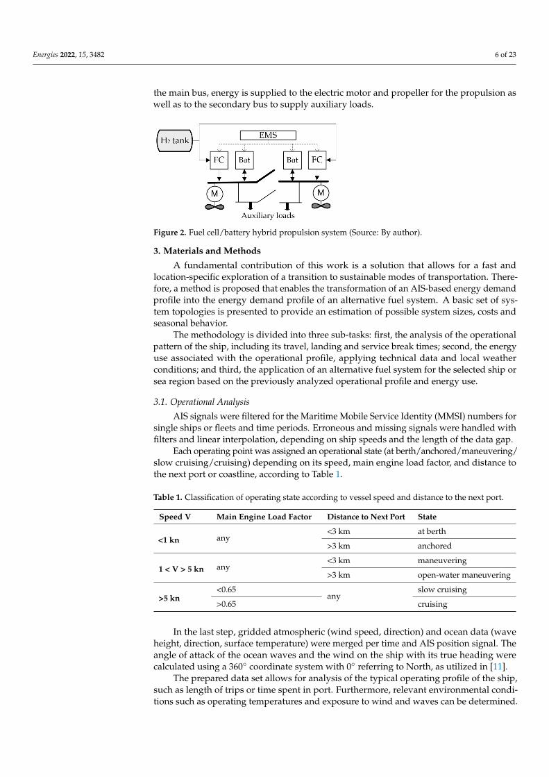
Energies 2022, 15, 3482 6 of 23

the main bus, energy is supplied to the electric motor and propeller for the propulsion aswell as to the secondary bus to supply auxiliary loads.

Energies 2022, 15, x FOR PEER REVIEW 6 of 23

electricity bus. From the main bus, energy is supplied to the electric motor and propeller for the propulsion as well as to the secondary bus to supply auxiliary loads.

Figure 2. Fuel cell/battery hybrid propulsion system (Source: By author).

3. Materials and Methods A fundamental contribution of this work is a solution that allows for a fast and loca-

tion-specific exploration of a transition to sustainable modes of transportation. Therefore, a method is proposed that enables the transformation of an AIS-based energy demand profile into the energy demand profile of an alternative fuel system. A basic set of system topologies is presented to provide an estimation of possible system sizes, costs and sea-sonal behavior.

The methodology is divided into three sub-tasks: first, the analysis of the operational pattern of the ship, including its travel, landing and service break times; second, the en-ergy use associated with the operational profile, applying technical data and local weather conditions; and third, the application of an alternative fuel system for the selected ship or sea region based on the previously analyzed operational profile and energy use.

3.1. Operational Analysis AIS signals were filtered for the Maritime Mobile Service Identity (MMSI) numbers

for single ships or fleets and time periods. Erroneous and missing signals were handled with filters and linear interpolation, depending on ship speeds and the length of the data gap.

Each operating point was assigned an operational state (at berth/anchored/maneu-vering/slow cruising/cruising) depending on its speed, main engine load factor, and dis-tance to the next port or coastline, according to Table 1.

Table 1. Classification of operating state according to vessel speed and distance to the next port.

Speed V Main Engine Load Factor Distance to Next Port State

<1 kn any <3 km at berth >3 km anchored

1 < V > 5 kn any <3 km maneuvering

>3 km open-water maneu-vering

>5 kn <0.65

any slow cruising

>0.65 cruising

In the last step, gridded atmospheric (wind speed, direction) and ocean data (wave height, direction, surface temperature) were merged per time and AIS position signal. The angle of attack of the ocean waves and the wind on the ship with its true heading were calculated using a 360° coordinate system with 0° referring to North, as utilized in [11].

The prepared data set allows for analysis of the typical operating profile of the ship, such as length of trips or time spent in port. Furthermore, relevant environmental condi-tions such as operating temperatures and exposure to wind and waves can be determined.

Figure 2. Fuel cell/battery hybrid propulsion system (Source: By author).

3. Materials and Methods

A fundamental contribution of this work is a solution that allows for a fast andlocation-specific exploration of a transition to sustainable modes of transportation. There-fore, a method is proposed that enables the transformation of an AIS-based energy demandprofile into the energy demand profile of an alternative fuel system. A basic set of sys-tem topologies is presented to provide an estimation of possible system sizes, costs andseasonal behavior.

The methodology is divided into three sub-tasks: first, the analysis of the operationalpattern of the ship, including its travel, landing and service break times; second, the energyuse associated with the operational profile, applying technical data and local weatherconditions; and third, the application of an alternative fuel system for the selected ship orsea region based on the previously analyzed operational profile and energy use.

3.1. Operational Analysis

AIS signals were filtered for the Maritime Mobile Service Identity (MMSI) numbers forsingle ships or fleets and time periods. Erroneous and missing signals were handled withfilters and linear interpolation, depending on ship speeds and the length of the data gap.

Each operating point was assigned an operational state (at berth/anchored/maneuvering/slow cruising/cruising) depending on its speed, main engine load factor, and distance tothe next port or coastline, according to Table 1.

Table 1. Classification of operating state according to vessel speed and distance to the next port.

Speed V Main Engine Load Factor Distance to Next Port State

<1 kn any<3 km at berth

>3 km anchored

1 < V > 5 kn any<3 km maneuvering

>3 km open-water maneuvering

>5 kn<0.65

anyslow cruising

>0.65 cruising

In the last step, gridded atmospheric (wind speed, direction) and ocean data (waveheight, direction, surface temperature) were merged per time and AIS position signal. Theangle of attack of the ocean waves and the wind on the ship with its true heading werecalculated using a 360◦ coordinate system with 0◦ referring to North, as utilized in [11].

The prepared data set allows for analysis of the typical operating profile of the ship,such as length of trips or time spent in port. Furthermore, relevant environmental condi-tions such as operating temperatures and exposure to wind and waves can be determined.

Energies 2022, 15, 3482 7 of 23

3.2. Energy Use Prediction3.2.1. Ship Technical Parameters

For energy use prediction, ship technical parameters such as dimensions and motoriza-tion were required. Some parameters are mandatory; others can be replaced with statisticaldata, as shown in Appendix A, Table A1.

3.2.2. Speed Penalties

At each operating point, the speed penalty ∆v/v was calculated for the effects of oceanwaves, wind, shallow waters and hull fouling. For the penalty of ocean waves ∆v/vsw themodel of Townsin and Kwon [42] was utilized with the formula for cargo ships and a blockcoefficient in the range of 0.55–0.7, considering the angle of attack of the ocean waves.

Added resistance by wind ∆RW was calculated on the basis established by Blender-mann, utilizing the drag coefficient profile for RoPax ships [43] and transposed to the windspeed penalty ∆v/vw with the total expected resistance RT based on Harvald [44] accordingto Equation (8) [23]:

∆vv w

=

(1 +

∆RWRT

) 12− 1 (9)

A shallow water speed penalty ∆v/vsh was applied according to Lackenby [45] withan average expected water depth, especially relevant for channels and rivers.

Hull fouling was addressed with a constant factor of 0.18 on the ITTC-1957 hull frictioncoefficient [46], based on the findings of Aertssen [47], described in [23].

The speed penalty for hull fouling ∆v/v f was obtained similarly to Equation (9). Thetotal speed penalty ∆v/v is given by the total influence of waves, wind, shallow water andhull fouling:

∆vv

=∆vv sw

+∆vv w

+∆vv sh

+∆vv f

(10)

3.2.3. Main Engine Power

The power output of the main engine was calculated for each operating point withEquation (3), considering the current ship draught (if provided by AIS data), ship speedand speed penalty due to real sea conditions. The installed engine power PME, inst wasscaled by εP to the reference power if information on appropiate scaling was available.Otherwise, PME, inst was used as Pre f .

3.2.4. Auxiliary Engine Power

Installed auxiliary engine capacity PAE, inst was estimated with a factor of 0.278 inPME, inst, based on [48]. Load factors LFAE per operating state, as used in Equation (4), weredeveloped based on data from the MV Shapinsay, the basis vessel for HySeas III [34]. Valueswere differentiated between three different comfort classes depending on the onboardfacilities, as shown in Appendix A, Table A2.

3.2.5. Total Fuel Consumption and Emissions

The total consumed fuel mass m f uel and the emission masses mp for each pollutantwere calculated with Equations (5) and (7). Fuel and external costs could be derived usingcost factors and the total masses.

3.3. Low-Carbon Technology Transition

The operational profile, energy use and local renewable energy potential were utilizedfor the sizing of fuel system components, ship propulsion system, fuel station, storage,electrolysis and wind farm, as shown in Figure 3. The CAPital EXpenditures (CAPEX) werederived from the sizes of the components and the OPerational EXpenditures (OPEX) andemissions from the demand-driven operation of the fuel system. Finally, the Levelized Costs

Energies 2022, 15, 3482 8 of 23

Of Transportation (LCOT) could be calculated. In the following, the different conversionsteps for component sizing are described.

Energies 2022, 15, x FOR PEER REVIEW 8 of 23

storage, electrolysis and wind farm, as shown in Figure 3. The CAPital EXpenditures (CAPEX) were derived from the sizes of the components and the OPerational EXpendi-tures (OPEX) and emissions from the demand-driven operation of the fuel system. Finally, the Levelized Costs Of Transportation (LCOT) could be calculated. In the following, the different conversion steps for component sizing are described.

Figure 3. Transfer scheme for the operational profile and energy use of a RoPax ferry, as well as the renewable energy potential of a low-carbon fuel system (Source: By author).

3.3.1. Fuel Cell Hybrid Propulsion System The fuel cell was sized such that it was able to deliver sufficient power for stable

cruising at the ship’s reference speed, i.e., to deliver 𝑃 at an appropriate fuel cell load factor 𝐿𝐹 , , according to Equation (11): 𝑃 = 𝑃𝐿𝐹 , (11)

The necessary on-board energy storage was the maximum daily propulsive energy use 𝐸 , , . The designed (des.) energy storage of hydrogen 𝑚 , . was derived us-ing the degree of hybridization 𝑓 , i.e., the energetic contribution of the battery to the pro-pulsive energy depending on the EMS, as well as the fuel cell efficiency 𝜂 and lower heating value 𝐿𝐻𝑉 , according to Equation (12): 𝑚 , . = 𝐸 . ∗ (1 − 𝑓 )𝜂 ∗ 𝐿𝐻𝑉 (12)

The designed electric energy storage capacity 𝐸 , . was calculated considering the discharge efficiency 𝜂 and the minimum allowable state of charge (𝑆𝑂𝐶 ) as shown in Equation (13): 𝐸 , . = 𝐸 . ∗ 𝑓𝜂 ∗ 1 + 𝑆𝑂𝐶(1 − 𝑆𝑂𝐶 ) (13)

3.3.2. Fuel Station The hydrogen landside storage capacity 𝑚 was the designed on-board capacity 𝑚 , . multiplied by the days required for safe storage 𝑑 as shown in Equation (14):

Figure 3. Transfer scheme for the operational profile and energy use of a RoPax ferry, as well as therenewable energy potential of a low-carbon fuel system (Source: By author).

3.3.1. Fuel Cell Hybrid Propulsion System

The fuel cell was sized such that it was able to deliver sufficient power for stablecruising at the ship’s reference speed, i.e., to deliver Pre f at an appropriate fuel cell loadfactor LFFCS,re f , according to Equation (11):

PFC =Pre f

LFFCS,re f(11)

The necessary on-board energy storage was the maximum daily propulsive energy useEP,daily, max. The designed (des.) energy storage of hydrogen mH2, des. was derived using thedegree of hybridization fh, i.e., the energetic contribution of the battery to the propulsiveenergy depending on the EMS, as well as the fuel cell efficiency ηFC and lower heatingvalue LHVH2, according to Equation (12):

mH2, des. =Edes. ∗ (1 − fh)

ηFC ∗ LHVH2(12)

The designed electric energy storage capacity EE,des. was calculated considering thedischarge efficiency ηBd and the minimum allowable state of charge (SOCmin) as shown inEquation (13):

EE,ds. =Edes. ∗ fh

ηBd

∗(

1 +SOCmin

(1 − SOCmin)

)(13)

3.3.2. Fuel Station

The hydrogen landside storage capacity mSt was the designed on-board capacitymH2, des. multiplied by the days required for safe storage dSt as shown in Equation (14):

mSt = mH2, des. ∗ dSt (14)

Energies 2022, 15, 3482 9 of 23

The compressor power PC (non-cascaded) was sized based on the required maximumfueling rate

.m, according to fueling time restrictions and the minimum source pressure

pmin of the hydrogen storage system, which could be a tube-trailer, low-pressure storagesystem or pipeline, as considered in Equation (15):

PC =.

m ∗ 1ηC

∗ T ∗k ∗ RH2

k − 1∗[

p1

pmin− 1]

(15)

Which also required the compressor efficiency ηC, the source temperature T, thehydrogen specific heat relation k and the gas constant of hydrogen RH2 as well as theon-board tank target pressure p1.

If landside charging of the ship’s battery was utilized, the required power PCh wasaligned to the optimal battery charge rate (C-rate) rc,opt:

PCh = Edes. ∗ fh ∗ rc,opt (16)

With charging time restrictions, the C-rate could increase to a maximum of 1.

3.3.3. Electrolysis

The daily target production capacity mH2, EL,design considered the buffering effect ofthe storage dSt. A rolling mean of dSt was applied to the daily hydrogen consumption andits maximum was mH2, EL,des.. This quantity was estimated using Equation (17):

mH2, EL,des. = max

(1ds

∗dSt

∑i=1

mH2,daily,i

)(17)

Moreover, the required electrolyser power PEL, based on the hydrogen higher heatingvalue HHVH2 , electrolyser efficiency ηEL and an average daily availability factor fa, wascalculated employing Equation (18):

PEL =mH2,EL,daily ∗ HHVH2

ηEL ∗ fa ∗ 24h(18)

3.3.4. Wind Farm

On a daily basis, the energy demand Etot of the fuel station facilities and electrolyserhad to be supplied by a wind farm operating at the local daily wind capacity factor CW ,according to Equation (19):

PW,req.,daily =Etot

24h ∗ CW(19)

The capacity factor CW was determined based on the daily wind speeds and a repre-sentative turbine model from the Python library windpowerlib [49].

The final size of the wind farm PW was determined considering the buffer effect witha rolling mean of the window dSt over PW,req.,daily. On a portion of rSS days, representingthe self-supply rate, the wind farm could provide the full energy. On a portion of 1 − rSSdays, grid electricity was added.

3.3.5. Levelized Costs of Transportation

For both systems, the base system and the alternative hydrogen system, levelized costsof transportation were calculated. The investment cost (CAPEX) and annual operating cost(OPEX) values of all system components were determined by cost factors, e.g., the nominalpower of a component or the consumed fuel mass. The cost factors were determinedbased on literature research and industry interviews, as documented in Appendix A.Additionally, for the hydrogen-based system, excess energy from the wind farm was fedinto the electricity grid, generating revenues RE. The prices per kWh were determinedby the average spot market and a supplemental renewable energy premium if applicable.

Energies 2022, 15, 3482 10 of 23

If a premium was part of the wind energy bidding process, e.g., as in Germany [50], anexponential decay (e(−0.5)) of the premium was assumed, with a major drop in the next fiveyears due to increasing competition.

Over the whole life span the LCOT were calculated using Equation (20):

LCOT =∑lc

t=1 CAPEX + OPEXt − RE,t

∑lct=1 dt

(20)

including the life cycle length lc, investment cost CAPEX, annual operating cost OPEXt,feed-in revenues RE,t and distance dt. The cost of capital was neglected in the LCOTcal-culation, as that relied on financial and political aspects, which are outside the scope ofthis model.

3.4. Implementation

The methodology was incorporated into a model coded in the open-source program-ming language Python, named ‘ELS-Energy Lighthouse Software’. Due to company policies,the tool is only available for internal use.

4. Case Study

In a case study, the impact of using a hydrogen fuel system for two RoPax vesselswas explored. These were the Earl Thorfinn, operating on various routes on the OrkneyIslands, and the Frisia III, connecting the German island of Norderney with the mainland.The two ferries were selected due to the availability of fuel consumption data, allowingfor the validation of the energy use estimation scheme. Furthermore, the sensitive naturalenvironments of these ferries imply the use of alternative fuels in the future.

The analysis was conducted with a data basis of the year 2020, containing AIS trackingdata, weather data, local wind energy capacities and ship technical data. Basic characteris-tics of the two vessels, as described in public web sources, are shown in Table 2.

Table 2. Ship technical data for the two case study vessels, including Maritime Mobile ServiceIdentifier (MMSI) and basic dimensions.

Unit Earl Thorfinn Frisia III

MMSI - 232,000,760 211,692,820

Length M 45.3 74.4

Breath M 12.2 13.4

Gross Tonnage Mt 771 1786

Speed Kn 12 12

Power kW 1486 1292

Passengers - 191 1338

Lane-Meters m 22 120

One can note that the installed capacity of the Earl Thorfinn exceeded that of the FrisiaIII, despite being a much smaller vessel, which can be ascribed to the harsher operatingconditions on the Orkney Islands. Further parameters specific to the case study, as wellas conversion factors utilized in the sizing and costs calculations, can be found in the fullparameter set in Appendix A, Table A3.

4.1. Operational Analysis

First, the operation of the two vessels was analyzed, identifying their routes of op-eration, vessel speed, service patterns and typical times of port calls by tracking the AISsignals. Figure 4 shows one crossing of the Frisia III between its main port of Norddeich

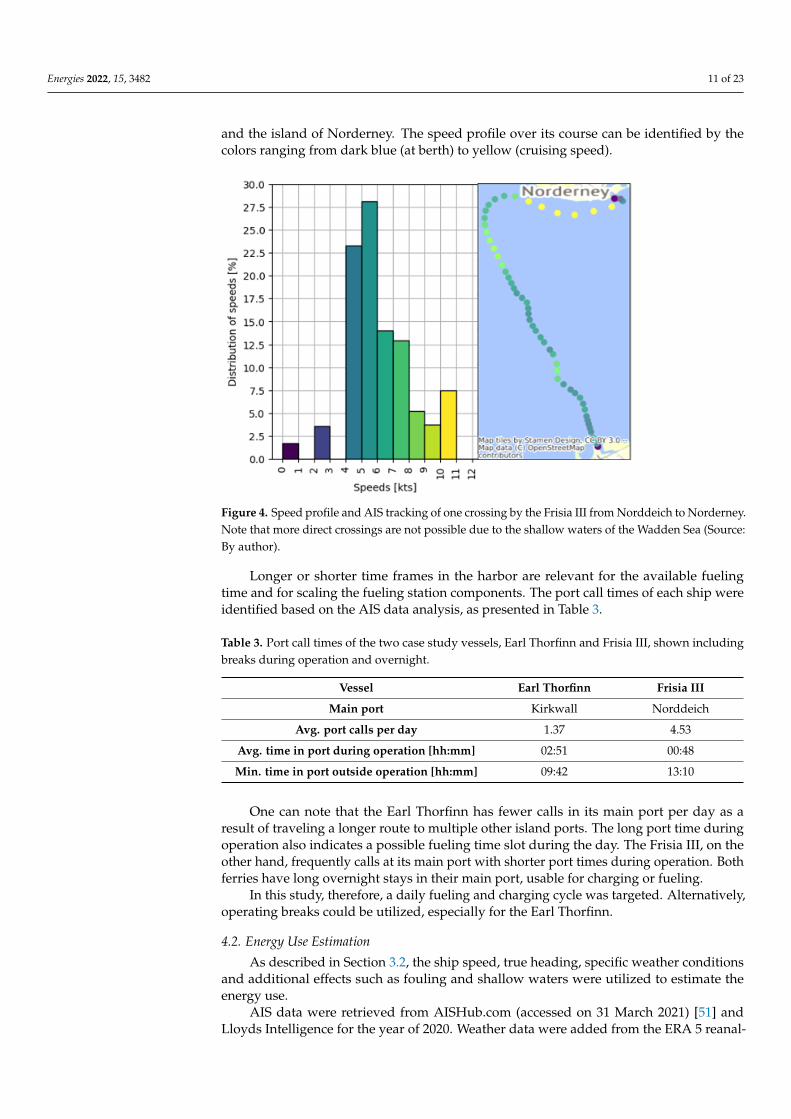
Energies 2022, 15, 3482 11 of 23

and the island of Norderney. The speed profile over its course can be identified by thecolors ranging from dark blue (at berth) to yellow (cruising speed).

Energies 2022, 15, x FOR PEER REVIEW 11 of 23

signals. Figure 4 shows one crossing of the Frisia III between its main port of Norddeich and the island of Norderney. The speed profile over its course can be identified by the colors ranging from dark blue (at berth) to yellow (cruising speed).

Figure 4. Speed profile and AIS tracking of one crossing by the Frisia III from Norddeich to Nor-derney. Note that more direct crossings are not possible due to the shallow waters of the Wadden Sea (Source: By author).

Longer or shorter time frames in the harbor are relevant for the available fueling time and for scaling the fueling station components. The port call times of each ship were iden-tified based on the AIS data analysis, as presented in Table 3.

Table 3. Port call times of the two case study vessels, Earl Thorfinn and Frisia III, shown including breaks during operation and overnight.

Vessel Earl Thorfinn Frisia III Main port Kirkwall Norddeich

Avg. port calls per day 1.37 4.53 Avg. time in port during operation

[hh:mm] 02:51 00:48

Min. time in port outside operation [hh:mm]

09:42 13:10

One can note that the Earl Thorfinn has fewer calls in its main port per day as a result of traveling a longer route to multiple other island ports. The long port time during oper-ation also indicates a possible fueling time slot during the day. The Frisia III, on the other hand, frequently calls at its main port with shorter port times during operation. Both fer-ries have long overnight stays in their main port, usable for charging or fueling.

In this study, therefore, a daily fueling and charging cycle was targeted. Alterna-tively, operating breaks could be utilized, especially for the Earl Thorfinn.

Figure 4. Speed profile and AIS tracking of one crossing by the Frisia III from Norddeich to Norderney.Note that more direct crossings are not possible due to the shallow waters of the Wadden Sea (Source:By author).

Longer or shorter time frames in the harbor are relevant for the available fuelingtime and for scaling the fueling station components. The port call times of each ship wereidentified based on the AIS data analysis, as presented in Table 3.

Table 3. Port call times of the two case study vessels, Earl Thorfinn and Frisia III, shown includingbreaks during operation and overnight.

Vessel Earl Thorfinn Frisia III

Main port Kirkwall Norddeich

Avg. port calls per day 1.37 4.53

Avg. time in port during operation [hh:mm] 02:51 00:48

Min. time in port outside operation [hh:mm] 09:42 13:10

One can note that the Earl Thorfinn has fewer calls in its main port per day as aresult of traveling a longer route to multiple other island ports. The long port time duringoperation also indicates a possible fueling time slot during the day. The Frisia III, on theother hand, frequently calls at its main port with shorter port times during operation. Bothferries have long overnight stays in their main port, usable for charging or fueling.

In this study, therefore, a daily fueling and charging cycle was targeted. Alternatively,operating breaks could be utilized, especially for the Earl Thorfinn.

4.2. Energy Use Estimation

As described in Section 3.2, the ship speed, true heading, specific weather conditionsand additional effects such as fouling and shallow waters were utilized to estimate theenergy use.

AIS data were retrieved from AISHub.com (accessed on 31 March 2021) [51] andLloyds Intelligence for the year of 2020. Weather data were added from the ERA 5 reanal-

Energies 2022, 15, 3482 12 of 23

ysis database of the European Centre for Medium-Range Weather Forecasts. A seabedtopography model is not yet incorporated into the model. Therefore, an average water-depth of 5 m was assumed for the shallow waters of the Wadden Sea, relevant for energyuse calculation for the Frisia III. Figure 5 depicts the daily energy use, with error bars pre-sented based on the assumption of full AIS availability and no loss of signal. The standarddeviation of the calculated propulsive power from the model is up to 18%, depending on er-rors in speed, wave and draught measurement and the specified reference power. The EarlThorfinn showed higher variation in energy use, with typical values ranging from 1–3.5 tof diesel fuel per week, while the Frisia III averaged approximately 1.5 t/week. Longerperiods out of operation could be noticed for the Frisia III as an effect of the COVID-19pandemic and the associated lockdown measures in the year 2020. As the operation duringthe summer months, when the islands are most frequented, reached regular operation,data from the year 2020 are still suitable for sizing the production and storage capacitiesof a hydrogen fuel system. Nevertheless, this poses limitations regarding adapting to theseasonal variation. Over the full course of the year, the Frisia III reached slightly highervalues in energy use and fuel consumption with 2328 MWh and 468 t, compared to the EarlThorfinn with 2229 MWh and 430 t (see also Figure 5).

Energies 2022, 15, x FOR PEER REVIEW 12 of 23

4.2. Energy Use Estimation As described in Section 3.2, the ship speed, true heading, specific weather conditions

and additional effects such as fouling and shallow waters were utilized to estimate the energy use.

AIS data were retrieved from AISHub.com (accessed on 31 March 2021) [51] and Lloyds Intelligence for the year of 2020. Weather data were added from the ERA 5 reanal-ysis database of the European Centre for Medium-Range Weather Forecasts. A seabed topography model is not yet incorporated into the model. Therefore, an average water-depth of 5 m was assumed for the shallow waters of the Wadden Sea, relevant for energy use calculation for the Frisia III. Figure 5 depicts the daily energy use, with error bars presented based on the assumption of full AIS availability and no loss of signal. The stand-ard deviation of the calculated propulsive power from the model is up to 18%, depending on errors in speed, wave and draught measurement and the specified reference power. The Earl Thorfinn showed higher variation in energy use, with typical values ranging from 1–3.5 t of diesel fuel per week, while the Frisia III averaged approximately 1.5 t/week. Longer periods out of operation could be noticed for the Frisia III as an effect of the COVID-19 pandemic and the associated lockdown measures in the year 2020. As the op-eration during the summer months, when the islands are most frequented, reached regu-lar operation, data from the year 2020 are still suitable for sizing the production and stor-age capacities of a hydrogen fuel system. Nevertheless, this poses limitations regarding adapting to the seasonal variation. Over the full course of the year, the Frisia III reached slightly higher values in energy use and fuel consumption with 2328 MWh and 468 t, compared to the Earl Thorfinn with 2229 MWh and 430 t (see also Figure 5).

Figure 5. Fuel consumption, in tons per day, of the Earl Thorfinn and Frisia III in the year 2020 (Source: By author).

The estimated fuel consumption values were contrasted against real consumption data for both ships. In the case of the Earl Thorfinn, the estimated consumption was 91.8% of the real consumption, whereas for the Frisia III it exceeded real consumption by 2.1%. Therefore, the model underestimated consumption in the former case and overestimated it in the latter case. Major daily offsets for the Earl Thorfinn were caused by the loss of the AIS signal as a result of transceiver malfunction, signal blocking or insufficient coverage of the terrestrial antennas. Smaller gaps in AIS signals could be addressed by linear inter-polation, while larger gaps distort the energy use profile. For future improvement, these gaps could be filled by replicating the typical operational profile per weekday. Further distortions could be observed on days of severe weather impact. This can be explained by the high sensitivity of ship propulsive power to wave height. Wave height data, obtained in this study from the ECMWF, were only available with a raster size of 55.5 km × 55.5

Figure 5. Fuel consumption, in tons per day, of the Earl Thorfinn and Frisia III in the year 2020(Source: By author).

The estimated fuel consumption values were contrasted against real consumptiondata for both ships. In the case of the Earl Thorfinn, the estimated consumption was 91.8%of the real consumption, whereas for the Frisia III it exceeded real consumption by 2.1%.Therefore, the model underestimated consumption in the former case and overestimated itin the latter case. Major daily offsets for the Earl Thorfinn were caused by the loss of the AISsignal as a result of transceiver malfunction, signal blocking or insufficient coverage of theterrestrial antennas. Smaller gaps in AIS signals could be addressed by linear interpolation,while larger gaps distort the energy use profile. For future improvement, these gaps couldbe filled by replicating the typical operational profile per weekday. Further distortions couldbe observed on days of severe weather impact. This can be explained by the high sensitivityof ship propulsive power to wave height. Wave height data, obtained in this study fromthe ECMWF, were only available with a raster size of 55.5 km × 55.5 km. Therefore, localphenomena, especially in bays, might not be precisely represented. Further sources of biasmay include imprecise ship technical data, deviations in the cubic relationship of powerto speed due to specific vessel characteristics, and other environmental impacts such asocean currents.

Energies 2022, 15, 3482 13 of 23

4.3. Hydrogen Fuel System

An alternative fuel system should be able to secure the required energy use of trans-portation throughout the year and with seasonal fluctuations. Local aspects were thereforeconsidered while parameterizing the model. For instance, the offshore wind farm locationnorth of Norderney was assumed to be the primary energy source in the Frisia scenario.For the Earl Thorfinn on the Orkneys, onshore energy installations were considered. Bothscenarios use electrolysis in a demand-driven operation to produce hydrogen. For theFrisia III, it was chosen for electrolysis to be operated close to the harbor, feeding into alow-pressure storage system. For the Earl Thorfinn, hydrogen production was assumed tobe off-site and transported via tube-trailers to the harbor over a range of <50 km.

4.3.1. System Sizing and Energy Balance

The fuel system components were sized using the basic scheme presented in Section 3.Conversion parameters of the individual fuel system components, such as efficiencies,hydrogen storage conditions, gravimetric and volumetric sizing factors, and cost factors,can be found in the case study-specific parameter set of Appendix A, Table A3. In Table 4,partial results are shown for the wind farm, electrolysis, buffer storage, compression unitand onboard hydrogen storage capacity.

Table 4. Partial results of hydrogen fuel system component sizing for the Earl Thorfinn and Frisia III.

Sizing Parameter Earl Thorfinn Frisia III

Wind farm capacity PW [MW] 4.0 3.4

Electrolyser capacity PELY [MW] 2.21 1.7

Hydrogen fuel station gravimetric storage capacity mSt [kg] 1800 1246

Fueling compressor capacity PC [MW] 0.75 1.25

Onboard hydrogen gravimetric capacity mH2,des. [kg] 882 684

The required capacity of the windfarm was determined including a buffering effectof the hydrogen storage and based on the energy autonomy criteria of 80% of the days.Appendix B, Figure A1 indicates the required capacities for lower or higher self-supplyrates. Appendix B, Figure A2 shows the balance of generated and used energy of thesystems. Despite the similar annual energy use, as shown in Figure 5, the renewable sourcein the Orkney scenario requires higher capacities for the wind farm PW , electrolysis systemPELY and hydrogen storage system mSt. This is a result of the much higher fluctuations andhigher daily peak energy use of the ship (see also Figure 5 and Appendix B, Figure A2). Amore stable energy use profile, such as for the Frisia III, is beneficial for efficient sizing. Forthe compressor at the fuel station, the opposite can be observed. A much larger capacity isrequired as a result of the low source pressure, 50 bar, of the low-pressure hydrogen storage,as opposed to the 250 bar of the tube-trailer transport. Longer compression times at theelectrolysis station compared to the hydrogen fueling time at the fuel station allow for anoverall lower compression capacity. While both paths, tube-trailers combined with smallercompression capacity versus low-pressure storage with larger compression capacity, lead tosufficient fueling rates, the optimum configuration in each specific case will depend on thelocal availability of space as well as the distance between electrolyser and fueling station,which is outside the scope of this work.

In conclusion, it can be stated that the presented scheme allocates a sufficient energysource and fuel conversion system for a ship’s energy use. For future work, the schemecould be extended by optimizing the size relations within the fuel conversion path.

4.3.2. CAPEX, OPEX and Wind Energy Revenues

The total investment costs of both systems differ significantly with 15.92 million EURfor the Earl Thorfinn compared to 26.25 million EUR for the Frisia III. The most significant

Energies 2022, 15, 3482 14 of 23

difference can be seen in the proportion of the wind farm costs within the total investmentcosts (Figure 6). Besides the wind farm, the remaining proportions of system costs wereallocated similarly in both cases, with costs of the fuel cell system being dominant, followedby the costs of electrolysis and the fuel station system. The supplementary systems onboard of the ship, such as the balancing battery, hydrogen tank, electrical grid and auxiliarysystems, added up to approximately 60% of the costs of the fuel cell system.

Energies 2022, 15, x FOR PEER REVIEW 14 of 23

In conclusion, it can be stated that the presented scheme allocates a sufficient energy source and fuel conversion system for a ship’s energy use. For future work, the scheme could be extended by optimizing the size relations within the fuel conversion path.

4.3.2. CAPEX, OPEX and Wind Energy Revenues The total investment costs of both systems differ significantly with 15.92 million EUR

for the Earl Thorfinn compared to 26.25 million EUR for the Frisia III. The most significant difference can be seen in the proportion of the wind farm costs within the total investment costs (Figure 6). Besides the wind farm, the remaining proportions of system costs were allocated similarly in both cases, with costs of the fuel cell system being dominant, fol-lowed by the costs of electrolysis and the fuel station system. The supplementary systems on board of the ship, such as the balancing battery, hydrogen tank, electrical grid and auxiliary systems, added up to approximately 60% of the costs of the fuel cell system.

(a) (b)

Figure 6. Estimated fuel system cost proportions: (a) Earl Thorfinn at a total CAPEX of 15.92 million EUR, (b) Frisia III at a total CAPEX of 26.25 million EUR (Source: By author).

The difference in the cost structure was mainly driven by the type of wind farm. The Orkney Islands allow for positioning of the wind turbines on land, thereby making up only a third of the cost of an offshore installation. Similar findings apply to the system maintenance costs, which were 0.26 million EUR per annum for case 1 and 0.61 million EUR for case 2, where offshore wind farm maintenance was the major driver in OPEX.

In both cases, the hydrogen production is initiated based on demand and follows the energy use profile with the buffering effect of the hydrogen storage system. Excess energy from the wind turbines is fed into the grid, while energy deficits on days of low wind capacity have to be supplemented by the grid. The annual balance of fuel system energy use, wind energy produced and traded grid quantities is shown in Table 5.

Table 5. Wind farm energy production versus actual fuel system energy use and resulting excess energy balance.

Earl Thorfinn Frisia III Energy produced by wind farm [MWh/y] 18,474 20,164

Hydrogen fuel system total energy use [MWh/y] 7816 7943 Grid purchase [MWh/y] 1203 1053 Grid feed-in [MWh/y] 11,860 13,274

Excess wind energy revenues [M€/y] +0.174 +0.254

With a decreasing wind premium scheme, such as in the case of Frisia III, the finan-cial balance is only representative for the first year.

Figure 6. Estimated fuel system cost proportions: (a) Earl Thorfinn at a total CAPEX of 15.92 millionEUR, (b) Frisia III at a total CAPEX of 26.25 million EUR (Source: By author).

The difference in the cost structure was mainly driven by the type of wind farm. TheOrkney Islands allow for positioning of the wind turbines on land, thereby making uponly a third of the cost of an offshore installation. Similar findings apply to the systemmaintenance costs, which were 0.26 million EUR per annum for case 1 and 0.61 millionEUR for case 2, where offshore wind farm maintenance was the major driver in OPEX.

In both cases, the hydrogen production is initiated based on demand and follows theenergy use profile with the buffering effect of the hydrogen storage system. Excess energyfrom the wind turbines is fed into the grid, while energy deficits on days of low windcapacity have to be supplemented by the grid. The annual balance of fuel system energyuse, wind energy produced and traded grid quantities is shown in Table 5.

Table 5. Wind farm energy production versus actual fuel system energy use and resulting excessenergy balance.

Earl Thorfinn Frisia III

Energy produced by wind farm [MWh/y] 18,474 20,164

Hydrogen fuel system total energy use [MWh/y] 7816 7943

Grid purchase [MWh/y] 1203 1053

Grid feed-in [MWh/y] 11,860 13,274

Excess wind energy revenues [M€/y] +0.174 +0.254

With a decreasing wind premium scheme, such as in the case of Frisia III, the financialbalance is only representative for the first year.

In both cases, the criteria of over 80% energy autonomy is met; however, a ma-jor portion of the produced energy is fed into the grid, achieving 42.3% and 39.4% self-consumption, respectively, of produced wind energy.

To increase self-consumption and the effective use of infrastructure, a larger hydrogenstorage than the two-day buffer would be required. Furthermore, the interaction amongavailable wind energy, electrolysis and current spot market price could be optimized byconsidering hourly instead of daily values, which is outside the scope of this work.

Energies 2022, 15, 3482 15 of 23

4.3.3. Emissions

Through implementing a hydrogen fuel system, the CO2, NOx, SOx, and PM2.5emissions and related external costs for both scenarios could be reduced significantlycompared to the diesel base case, as shown in Table 6. The overall reduction in externalemission costs was above 95% in both cases.

Table 6. Emission reductions through implementation of a hydrogen fuel system.

Scenario Parameter Earl Thorfinn Frisia III

Diesel use base [t/y] 430 468

CO2 mass base [t/y], at 0.260 t€/t 1409.1 1463

NOx mass base [t/y], at 12.6 t€/t 71.1 58.2

SOx base [t/y], at 4.3 t€/t 0.6 0.7

PM2.5 mass base [t/y], at 70.0 t€/t 1.0 1.1

Emission external costs [M€/y] 1.335 1.194

Expected CO2 tax [M€/y] 0.035 0.037

Hydrogen use altern. [t/y] 111.7 114.1

CO2 altern. [t/y], at 0.260 t€/t 211.0 214.4

Emission external costs [M€/y] 0.055 0.056

CO2 tax altern. [M€/y] 0.005 0.005

Hydrogen fuel system external emission cost savings [%] 95.9% 95.3%

CO2 tax savings [%] 85.7% 86.5%

Due to similar energy use, the emission levels of both ships remained comparable. Theolder combustion engine technology of the Earl Thorfinn leads to higher NOx emissionsand increased emissions costs compared to the Frisia III.

4.3.4. Levelized Costs of Transportation (LCOT)

By calculating the LCOT, investment as well as operational cost can be comparedbetween the base and the alternative system over the whole lifespan. A typical life cyclebasis of 20 years for maritime applications, for both the diesel base case and the alternativehydrogen system, was assumed. Figure 7a depicts the LCOT for both vessels in the basecase as well as the hydrogen fuel system case. With external emissions costs, the overallLCOT of the base cases exceeded those of the hydrogen fuel systems. Without these costs,the overall LCOT were lower. For hydrogen cases, the costs of the wind farm could becompensated for by revenues from excess wind energy to a full or partial extension. ForFrisia III, the LCOT of hydrogen did not reach a comparable level to the base case.

For comparison, the fuel system was calculated without including a wind farm utiliz-ing grid energy at an average price of 10 ct/kWh, as shown in Figure 7b.

The comparison of LCOT between a full hydrogen fuel system (see Figure 7a) andan approach utilizing grid electricity (Figure 7b) demonstrates a financial benefit fromincluding a wind farm in the local energy system. This coincides with the expectation of asynergetic effect due to balancing wind energy fluctuations with hydrogen storage. On theother hand, it can be seen that hydrogen fuel systems cannot be financially competitive withconventional fueling with diesel on a full or partial system approach. However, furtheroptimization of the system configuration may decrease the LCOT of the hydrogen system.

Energies 2022, 15, 3482 16 of 23Energies 2022, 15, x FOR PEER REVIEW 16 of 23

(a) (b)

Figure 7. LCOT of a hydrogen fuel system, (a) including wind farm, electrolysis, storage, fueling system and fuel cell propulsion system, (b) without wind farm and using grid electricity for hydro-gen production at 10 ct/kWh (Source: By author).

For comparison, the fuel system was calculated without including a wind farm uti-lizing grid energy at an average price of 10 ct/kWh, as shown in Figure 7b.

The comparison of LCOT between a full hydrogen fuel system (see Figure 7a) and an approach utilizing grid electricity (Figure 7b) demonstrates a financial benefit from in-cluding a wind farm in the local energy system. This coincides with the expectation of a synergetic effect due to balancing wind energy fluctuations with hydrogen storage. On the other hand, it can be seen that hydrogen fuel systems cannot be financially competitive with conventional fueling with diesel on a full or partial system approach. However, fur-ther optimization of the system configuration may decrease the LCOT of the hydrogen system.

Autonomous fuel production and supply, including the wind farm, electrolyser and fuel station, exceeded the costs of diesel fuel sourcing. As already reflected in the system CAPEX (see Section 4.3.2), the wind farm was a major driver for LCOT as well, especially if an offshore application was utilized. Still, in the hydrogen scenario for the Earl Thorfinn, the high wind farm CAPEX could be compensated for by selling excess wind energy to the grid.

For the ship propulsion system, including the fuel cell, fuel tank, battery and auxilia-ries, LCOT tripled compared to the base case due to higher component costs. However, the component costs were applied at the level of the year 2020 and might decrease with further market penetration and scale of production.

In terms of emissions for both vessels, the hydrogen fuel systems brought major ben-efits in LCOT. However, the full external emissions costs are not covered by the operator; only the CO2 taxes are. Applying a linearly increasing price range of 25–125 EUR/t, CO2 taxes cover only a small extent of the actual external costs and have little effect on the overall LCOT.

5. Conclusions Because of their operation on stable routes, RoPax ferries are one of the vessel types

predestined for the integration of novel low-carbon technologies. In this research, a com-bined method for operational profile analysis, energy use prediction and low-carbon fuel system transition modeling was developed, allowing for a fast assessment of routes or sea regions.

The methodology was tested on a case study of two appropriate vessels with the fol-lowing findings. Ship tracking using AIS data, as also employed in other studies, was a robust and highly effective method for ship operational analysis, given sufficient availa-bility of signals. The energy use prediction scheme from Jalkanen’s model STEAM I [16],

Figure 7. LCOT of a hydrogen fuel system, (a) including wind farm, electrolysis, storage, fuelingsystem and fuel cell propulsion system, (b) without wind farm and using grid electricity for hydrogenproduction at 10 ct/kWh (Source: By author).

Autonomous fuel production and supply, including the wind farm, electrolyser andfuel station, exceeded the costs of diesel fuel sourcing. As already reflected in the systemCAPEX (see Section 4.3.2), the wind farm was a major driver for LCOT as well, especially ifan offshore application was utilized. Still, in the hydrogen scenario for the Earl Thorfinn,the high wind farm CAPEX could be compensated for by selling excess wind energy tothe grid.

For the ship propulsion system, including the fuel cell, fuel tank, battery and auxil-iaries, LCOT tripled compared to the base case due to higher component costs. However,the component costs were applied at the level of the year 2020 and might decrease withfurther market penetration and scale of production.

In terms of emissions for both vessels, the hydrogen fuel systems brought majorbenefits in LCOT. However, the full external emissions costs are not covered by the operator;only the CO2 taxes are. Applying a linearly increasing price range of 25–125 EUR/t, CO2taxes cover only a small extent of the actual external costs and have little effect on theoverall LCOT.

5. Conclusions

Because of their operation on stable routes, RoPax ferries are one of the vessel typespredestined for the integration of novel low-carbon technologies. In this research, a com-bined method for operational profile analysis, energy use prediction and low-carbon fuelsystem transition modeling was developed, allowing for a fast assessment of routes orsea regions.

The methodology was tested on a case study of two appropriate vessels with thefollowing findings. Ship tracking using AIS data, as also employed in other studies,was a robust and highly effective method for ship operational analysis, given sufficientavailability of signals. The energy use prediction scheme from Jalkanen’s model STEAMI [16], extended with the effects of wind, hull fouling and shallow waters, was identified asthe most effective within the scope of the research. The standard deviation of the calculatedpropulsive power of the model was up to 18%, depending on errors in speed, wave anddraught measurement and the specified reference power. Upon applying the scheme ontwo case study vessels, the predicted energy use was within ±10% of the actual annual use.The energy use profile was used to model an alternative hydrogen-fueled system. For bothships, savings in emissions external costs on the order of 95% and savings in CO2 taxesabove 85% could be achieved, leading to decreases in the levelized costs of transportation(LCOT) of 58% and 24%, respectively, when considering external emission costs of the CO2,NOX, SOX and PM2.5 exhaust gas emissions. However, on a system cost basis only (not

Energies 2022, 15, 3482 17 of 23

considering external emission costs and only CO2 taxes), hydrogen-fueled systems at thecurrent state of technology were more expensive, though the price increase tremendouslydepended on the specific installation possibilities and renewable energy potential on site.

In the scenarios, only wind power was used as a renewable energy source, which inboth locations generated energy deficits in the summer months. For further investigations,this indicates the possibility of utilizing photovoltaic installations as a complementaryenergy source.

Integrating further vessel types that are relevant for renewable fueling will allow formodeling of hydrogen demand and supply systems containing various ship types to coverfull sea regions, and for demonstrating the scalability of the tool.

Furthermore, the model may be extended by including operation on rivers, bathymetrymaps of water depths, and consideration of currents. Additionally, the integration of otherlow-carbon fuels and renewable energy sources, as well as the integration of an excessenergy-driven approach, should be pursued. The developed tool ELS, which implementsthe proposed methodology, allows for the assessment of single ship routes or ship fleets,the outlining of pathways to more sustainable fuel systems with different scenario options,and the indication of local hydrogen demands.

Consequently, the presented methodology is able to support the decision processregarding pioneering future marine fuel systems in an appropriate manner.

Author Contributions: Conceptualization, J.C.G.T. and F.S.T.; methodology, A.C.F.; software, A.C.F.;validation, A.C.F.; formal analysis, A.C.F.; investigation, A.C.F. and J.C.G.T.; resources, F.S.T.; datacuration, A.C.F.; writing—original draft preparation, A.C.F.; writing—review and editing, J.C.G.T.and F.S.T.; visualization, A.C.F.; supervision, F.S.T. and J.C.G.T.; project administration, F.S.T. andJ.C.G.T. All authors have read and agreed to the published version of the manuscript.

Funding: This research received no external funding.

Institutional Review Board Statement: Not applicable.

Informed Consent Statement: Not applicable.

Data Availability Statement: Not applicable.

Acknowledgments: The authors would like to thank Reederei Frisia and Orkney Island Council—Ferry Services for their contributions of data for the validation of the methodology.

Conflicts of Interest: The authors declare no conflict of interest.

Appendix A

Table A1. Ship technical data required for energy use evaluation and replacement parameters thatcan be utilized if data are missing. Statistical values are determined based on data collected fromRoPax ferries by Kristensen et al. in 2016 [52].

Ship Technical Parameter Missing Parameter Replacement

MMSI

Mandatory parameters

Length overall

Breath

Gross tonnage

Dead weight, reference

Draught, reference

Ship speed, reference

Main engine power, reference

Energies 2022, 15, 3482 18 of 23

Table A1. Cont.

Ship Technical Parameter Missing Parameter Replacement

Main engine type(slow/medium/high-speed) Medium-speed diesel

ME model year 2000

ME fuel type Heavy fuel oil

AE power statistical

AE type Medium-speed diesel

AE model year 2000

AE fuel type Marine distillate oil

Midship section statistical

Table A2. Ship comfort class classification and resulting auxiliary engine load factors in differentstates of operation.

Ship Facilities Comfort Class At Berth Ma-Noeuvre Slow Cruising Cruising

Seating areawithout service low 0.46 0.67 0.55 0.28

Seating areawith service medium 0.535 9.745 0.625 0.38 (+10%)

Hotelingfacilities high 0.61 0.82 0.7 0.48 (+20%)

Table A3. Specific parameter set for the case study, presented in this paper, with sources or explana-tions for the values chosen.

Parameter Unit Value Source/BasisEmission external costs factors

CO2 cCO2 EUR/t 260 German Environmental Agency 2014 [53]. Mediumlong-term scenario (until 2050).

NOx cNOx EUR/t 12,600 TU Delft 2018 [4]Value for rural areas, as ships spend most of their

operation in open water.PM 2.5 cPM2.5 EUR/t 7000

SOx cSOx EUR/t 4300 Sanabra 2014 [54], lowest sensitivity.Fuel cell propulsion system

Degree of hybridization fh % 35 Aligned to Han 2014 [38]

Li-Ion battery charging efficiency ηBc % 90Valoen 2007 [55]

Li-Ion battery discharging efficiency ηBd % 85

Max. C-Rate discharge rd,max - 1 Scenario assumption

Opt. C-Rate charge rc,opt - 0.3 Scenario assumption

Fuel cell system efficiency ηFCS % 50 Van Biert 2016, PEM-Fuel cell [56]

Fuel cell load factor atreference speed LFFCS,re f % 70 Scenario assumption. For optimum range of

40–60% [38], operation at medium speeds.

Hydrogen tank ambient temperature T K 300 Scenario assumption for regular ambienttemperature

Hydrogen tank pressure p bar 600 Current on-road technology Rivard 2019,Table 3 [57]

Compressibility factor atstorage conditions ZH2 - 1.38 Cengel 2008 [58]

Energies 2022, 15, 3482 19 of 23

Table A3. Cont.

Parameter Unit Value Source/Basis

Lowest allowable hydrogentank pressure pH2,min bar 30

Similar empty tank pressure levels were used inHySeas III [34] and for the modeling of an on-road

fueling station by Reddi in 2014 [28].

Battery min. allowable SOC SOCmin % 30 Scenario assumption for optimum battery lifetime

Battery vol. energy density ρE, V kWh/l 0.3University of Washington 2020 [39]

Battery grav. energy density ρE,m kWh/kg 0.17

Fuel cell cost factor cFCS €/kW 1006 Estimate based on HySeas III project [34]

Hydrogen tank cost factor cFT €/kg 519 Current on-road technology Rivard 2019,Table 3 [57]

Li-Ion battery cost factor cB €/kWh 266.5 Cole 2021 [59]

Electric motor cost factor cEM €/kW 10.25 Lipman 1999 [60]

Installation cost factor ci % 20 Scenario assumptionFuel Station

Tube trailer capacity mT kg 600 Aliquo 2016 [32]

Days of storage safety dS d 2 Scenario assumption

Trailer cost factor per tank capacity cT €/kg 500Aliquo 2016 [32]

Max. pressure tube trailer pT,max bars 250

Min. pressure tube trailer pT,min bars 30Similar empty tank pressure levels were used inHySeas III and for the modeling of an on-road

fueling station by Reddi in 2014 [28,34]

Max. pressure low-pressure storage pS,max bars 50 Andersson 2019 [27]

Min. pressure low-pressure storage pS,min bars 10 Scenario assumption

Low-pressure storage cost cS €/kg 520 Parks 2014 [61]

Hydrogen grid pressure pg bars 100 Scenario assumption

Max. flow rate per dispenser.

mdisp. kg/s 0.05 HySeas III project [34]

Compressor isentropic efficiency ηC % 80 Parks 2014 [61]

Hydrogen source pressure p0 bars Dependent on storage type.

Hydrogen target pressure p1 bars 650 Hydrogen ship tank pressure +50 bars

Compressor cos ts based on flow rate.

m CC € 0.024283∗ .

m 0.5202 Weinert 2005 [62]

Cooling temperature TC K 253 Cooling level model for an on-road fueling stationby Reddi in 2014 [28].

Cooler coefficient of performance COP % 90 Cengel 2008 [58]

Charging facility cost factor cCh €/kW 205 Nicholas 2018 [63]

Fuel Station OPEX factor oFS%CA-

PEX/y 1 Scenario assumption.

Fuel station auxiliary systemsenergy use factor eFS % 10 Scenario assumption.

Electrolysis station

PEM Electrolyser efficiency ηEL % 80 Kumar 2019 [64] for PEM electrolyser, comparative70% for Alkaline

Electrolyser availability fa % 75 Scenario assumption.

Pressure after electrolysis pEL bar 15 Scenario assumption.

Electrolysis auxiliary systems costfactor faux % 10 Scenario assumption.

Energies 2022, 15, 3482 20 of 23

Table A3. Cont.

Parameter Unit Value Source/Basis

OPEX factor oEL %/y 1 Scenario assumption.

Electrolysis auxiliary systems energyuse factor eEL % 30 Scenario assumption for energy uses of water

purification, temperature managementWind farm

Days in buffer storage pipeline db d 5 Scenario assumption.

Minimum self-supply rate rSS % 80 Scenario assumption.

Wind energy feed in spot price tFI0.01

EUR/kWh 3.5 HySeas III project [34]

Offshore wind energy premium inGermany 2020 tFI,premium

0.01EUR/kWh 13.9 German Ministry of Economy and Climate

Protection [50]

Grid electricity price tP0.01

EUR/kWh 20 Scenario assumption.

Wind farm CAPEX factor cWP EUR/kW 1237/4100

On-shore Stehly 2018 [65]/Off-shore Voormolen2016 [66]

Wind farm OPEX factor oWP EUR/kW/y 37/109

On-shore Stehly 2018 [65]/Off-shore Voormolen2016 [66]

CO2 emissions factor forwind energy EFCO2,WE g/kWh 27 Thomson 2015 [67]

Appendix B

Energies 2022, 15, x FOR PEER REVIEW 20 of 23

Fuel station auxiliary systems energy use factor

𝑒 % 10 Scenario assumption.

Electrolysis station

PEM Electrolyser efficiency 𝜂 % 80 Kumar 2019 [64] for PEM

electrolyser, comparative 70% for Alkaline

Electrolyser availability 𝑓 % 75 Scenario assumption. Pressure after electrolysis 𝑝 bar 15 Scenario assumption.

Electrolysis auxiliary systems cost factor 𝑓 % 10 Scenario assumption. OPEX factor 𝑜 %/y 1 Scenario assumption.

Electrolysis auxiliary systems energy use factor

𝑒 % 30 Scenario assumption for energy uses

of water purification, temperature management

Wind farm Days in buffer storage pipeline 𝑑 d 5 Scenario assumption.

Minimum self-supply rate 𝑟 % 80 Scenario assumption.

Wind energy feed in spot price 𝑡 0.01 EUR/kWh

3.5 HySeas III project [34]

Offshore wind energy premium in Germany 2020

𝑡 , 0.01 EUR/kWh

13.9 German Ministry of Economy and Climate Protection [50]

Grid electricity price 𝑡 0.01 EUR/kWh

20 Scenario assumption.

Wind farm CAPEX factor 𝑐 EUR/kW 1237/ 4100

On-shore Stehly 2018 [65]/Off-shore Voormolen 2016 [66]

Wind farm OPEX factor 𝑜 EUR/kW/y 37/ 109

On-shore Stehly 2018 [65]/Off-shore Voormolen 2016 [66]

CO2 emissions factor for wind energy 𝐸𝐹 , g/kWh 27 Thomson 2015 [67]

Appendix B

Figure A1. Required wind farm size at different rates of fuel system autonomy, meaning the proportion of days the system is able to generate enough energy for fuel production.

Figure A1. Required wind farm size at different rates of fuel system autonomy, meaning the propor-tion of days the system is able to generate enough energy for fuel production.

Energies 2022, 15, 3482 21 of 23Energies 2022, 15, x FOR PEER REVIEW 21 of 23

(a) (b)

Figure A2. Hydrogen fuel system energy use and wind energy generation under the parameter set of Appendix A, Table A3, for the (a) Earl Thorfinn and (b) Frisia III.

References 1. European Commission. Roadmap to A Single European Transport Area—Towards a Competitive and Resource Efficient Transport

System; COM(2011) 144 Final; European Commission: Brussels, Belgium, 2011. Available online: https://eur-lex.europa.eu/LexUriServ/LexUriServ.do?uri=COM:2011:0144:FIN:en:PDF (accessed on 9 May 2022).

2. International Maritime Organization (IMO). Initial IMO Strategy on Reduction of GHG Emissions from Ships; MEPC.304(72): London, UK, 13 April 2018. Available online: https://unfccc.int/sites/default/files/resource/250_IMO%20submission_Talanoa%20Dialogue_April%202018.pdf (accessed on 9 May 2022).

3. Reşitoğlu, İ.A.; Altinişik, K.; Keskin, A. The pollutant emissions from diesel-engine vehicles and exhaust aftertreatment systems. Clean Technol. Environ. Policy 2015, 17, 15–27. https://doi.org/10.1007/s10098-014-0793-9.

4. Hoen, A.; Nieuwenhuijse, I.; de Bruyn, S. Health Impacts and Costs of Diesel Emissions in the EU; CE Delft: Delft, The Netherlands, 2018. Available online: https://cedelft.eu/publications/health-impacts-and-costs-of-diesel-emissions-in-the-eu/ (accessed 9 May 2022).

5. Petrospot Ltd. Session 4: Supply chain stakeholders have their say on the energy transition. In Proceedings of the Ship Energy Summit, Online, 8 September 2021.

6. Gómez Trillos, J.C. HySeas III—Market Potential Analysis of RoPax Ferry Market in Europe; Ref. Ares (2019)7435585; German Aerospace Centre (DLR): Oldenburg, Germany, 2019.

7. European Commission. THETIS-MRV CO2 Emission Report. Available online: https://mrv.emsa.europa.eu/#public/emission-report (accessed on 1 November 2020).

8. Cooper, J. Fuels Europe—Statistical Report 2019; FuelsEurope: Brussels, Belgium, 2019. Available online: https://www.fuelseurope.eu/publication/statistical-report-2019/ (accessed on 9 May 2022).

9. Kristensen, H.O.; Psaraftis, H. Energy Demand and Exhaust Gas Emissions of Marine Engines. 2015. Available online: https://www.danishshipping.dk/en/services/beregningsvaerktoejer/download/Basic_Model_Linkarea_Link/806/energy-demand-and-emissions-of-marine-engines-september-2015.pdf (accessed on 9 May 2022).

10. Winther, M.; Christensen, J.H.; Plejdrup, M.S.; Ravn, E.S.; Eriksson, F.; Kristensen, H.O. Emission inventories for ships in the arctic based on satellite sampled AIS data. Atmos. Environ. 2014, 91, 1–14. https://doi.org/10.1016/j.atmosenv.2014.03.006.

11. Jalkanen, J.-P.; Johansson, L.; Kukkonen, J.; Brink, A.; Kalli, J.; Stipa, T. Extension of an assessment model of ship traffic exhaust emissions for particulate matter and carbon monoxide. Atmos. Chem. Phys. 2012, 12, 2641–2659. https://doi.org/10.5194/acp-12-2641-2012.

12. Jalkanen, J.-P.; Johansson, L.; Kukkonen, J. A comprehensive inventory of the ship traffic exhaust emissions in the Baltic Sea from 2006 to 2009. Ambio 2014, 43, 311–324. https://doi.org/10.1007/s13280-013-0389-3.

13. Jalkanen, J.-P.; Johansson, L.; Kukkonen, J. A comprehensive inventory of ship traffic exhaust emissions in the European sea areas in 2011. Atmos. Chem. Phys. 2016, 16, 71–84. https://doi.org/10.5194/acp-16-71-2016.

14. International Maritime Organization (IMO). Third IMO Greenhouse Gas Study 2014. Available online: https://www.imo.org/en/OurWork/Environment/Pages/Greenhouse-Gas-Studies-2014.aspx (accessed on 9 May 2022).

Figure A2. Hydrogen fuel system energy use and wind energy generation under the parameter set ofAppendix A, Table A3, for the (a) Earl Thorfinn and (b) Frisia III.

References1. European Commission. Roadmap to A Single European Transport Area—Towards a Competitive and Resource Efficient Transport System;

COM(2011) 144 Final; European Commission: Brussels, Belgium, 2011; Available online: https://eur-lex.europa.eu/LexUriServ/LexUriServ.do?uri=COM:2011:0144:FIN:en:PDF (accessed on 5 May 2022).

2. International Maritime Organization (IMO). Initial IMO Strategy on Reduction of GHG Emissions from Ships; MEPC.304(72): London,UK, 13 April 2018; Available online: https://unfccc.int/sites/default/files/resource/250_IMO%20submission_Talanoa%20Dialogue_April%202018.pdf (accessed on 5 May 2022).

3. Resitoglu, I.A.; Altinisik, K.; Keskin, A. The pollutant emissions from diesel-engine vehicles and exhaust aftertreatment systems.Clean Technol. Environ. Policy 2015, 17, 15–27. [CrossRef]

4. Hoen, A.; Nieuwenhuijse, I.; de Bruyn, S. Health Impacts and Costs of Diesel Emissions in the EU; CE Delft: Delft, The Netherlands,2018; Available online: https://cedelft.eu/publications/health-impacts-and-costs-of-diesel-emissions-in-the-eu/ (accessed on5 May 2022).

5. Petrospot Ltd. Session 4: Supply chain stakeholders have their say on the energy transition. In Proceedings of the Ship EnergySummit, Online. 8 September 2021.

6. Gómez Trillos, J.C. HySeas III—Market Potential Analysis of RoPax Ferry Market in Europe; Ref. Ares (2019)7435585; GermanAerospace Centre (DLR): Oldenburg, Germany, 2019.

7. European Commission. THETIS-MRV CO2 Emission Report. Available online: https://mrv.emsa.europa.eu/#public/emission-report (accessed on 1 November 2020).

8. Cooper, J. Fuels Europe—Statistical Report 2019; FuelsEurope: Brussels, Belgium, 2019; Available online: https://www.fuelseurope.eu/publication/statistical-report-2019/ (accessed on 5 May 2022).

9. Kristensen, H.O.; Psaraftis, H. Energy Demand and Exhaust Gas Emissions of Marine Engines. 2015. Available online:https://www.danishshipping.dk/en/services/beregningsvaerktoejer/download/Basic_Model_Linkarea_Link/806/energy-demand-and-emissions-of-marine-engines-september-2015.pdf (accessed on 5 May 2022).

10. Winther, M.; Christensen, J.H.; Plejdrup, M.S.; Ravn, E.S.; Eriksson, F.; Kristensen, H.O. Emission inventories for ships in thearctic based on satellite sampled AIS data. Atmos. Environ. 2014, 91, 1–14. [CrossRef]

11. Jalkanen, J.-P.; Johansson, L.; Kukkonen, J.; Brink, A.; Kalli, J.; Stipa, T. Extension of an assessment model of ship traffic exhaustemissions for particulate matter and carbon monoxide. Atmos. Chem. Phys. 2012, 12, 2641–2659. [CrossRef]

12. Jalkanen, J.-P.; Johansson, L.; Kukkonen, J. A comprehensive inventory of the ship traffic exhaust emissions in the Baltic Sea from2006 to 2009. Ambio 2014, 43, 311–324. [CrossRef]

13. Jalkanen, J.-P.; Johansson, L.; Kukkonen, J. A comprehensive inventory of ship traffic exhaust emissions in the European sea areasin 2011. Atmos. Chem. Phys. 2016, 16, 71–84. [CrossRef]

14. International Maritime Organization (IMO). Third IMO Greenhouse Gas Study. 2014. Available online: https://www.imo.org/en/OurWork/Environment/Pages/Greenhouse-Gas-Studies-2014.aspx (accessed on 5 May 2022).

15. International Maritime Organization (IMO). Fourth IMO Greenhouse Gas Study. 2020. Available online: https://www.imo.org/en/OurWork/Environment/Pages/Fourth-IMO-Greenhouse-Gas-Study-2020.aspx (accessed on 9 April 2022).

Energies 2022, 15, 3482 22 of 23

16. Hydrogen Council. Path to Hydrogen Competitiveness—A Cost Perspective. 2020. Available online: https://hydrogencouncil.com/wp-content/uploads/2020/01/Path-to-Hydrogen-Competitiveness_Full-Study-1.pdf (accessed on 31 March 2021).

17. Aarskog, F.G.; Danebergs, J.; Strømgren, T.; Ulleberg, Ø. Energy and cost analysis of a hydrogen driven high speed passengerferry. Int. Shipbuild. Prog. 2020, 67, 97–123. [CrossRef]

18. Waldron Davies, C.; Harnisch, J.; Oswaldo, L.; Mckibbon, S.; Saile, S.; Wagner, F.; Walsh, M. 2006 IPCC Guidelines for NationalGreenhouse Gas Inventories; IPCC: Geneva, Switzerland, 2006.

19. Regulations for Carriage of AIS. International Maritime Organization (IMO). Available online: https://www.imo.org/en/OurWork/Safety/Pages/AIS.aspx (accessed on 3 March 2020).

20. Anwar, N. Navigation Advanced Mates, Masters, 1st ed.; Seamanship International: Lanarkshire, UK, 2006.21. MAN Energy Solutions. Basic Principles of Ship Propulsion; MAN Energy Solutions: Copenhagen, Denmark, 2018; Available

online: https://www.man-es.com/docs/default-source/marine/tools/basic-principles-of-ship-propulsion_web_links.pdf?sfvrsn=12d1b886_10 (accessed on 5 May 2022).

22. Jalkanen, J.-P.; Brink, A.; Kalli, J.; Pettersson, H.; Kukkonen, J.; Stipa, T. A modelling system for the exhaust emissions of marinetraffic and its application in the Baltic Sea area. Atmos. Chem. Phys. 2009, 9, 9209–9223. [CrossRef]

23. Molland, A.F.; Turnock, S.R.; Hudson, D.A. Ship Resistance and Propulsion: Practical Estimation of Ship Propulsive Power, 2nd ed.;Cambridge University Press: Cambridge, UK, 2017.

24. German Federal Ministry for Economic Affairs and Energy. The National Hydrogen Strategy. 2020. Available online: https://www.bmwk.de/Redaktion/EN/Publikationen/Energie/the-national-hydrogen-strategy.pdf?__blob=publicationFile&v=6 (ac-cessed on 5 May 2022).

25. Dincer, I. Green methods for hydrogen production. Int. J. Hydrogen Energy 2012, 37, 1954–1971. [CrossRef]26. Thema, M.; Bauer, F.; Sterner, M. Power-to-Gas: Electrolysis and methanation status review. Renew. Sustain. Energy Rev. 2019,

112, 775–787. [CrossRef]27. Andersson, J.; Grönkvist, S. Large-scale storage of hydrogen. Int. J. Hydrogen Energy 2019, 44, 11901–11919. [CrossRef]28. Reddi, K.; Elgowainy, A.; Sutherland, E. Hydrogen refueling station compression and storage optimization with tube-trailer

deliveries. Int. J. Hydrogen Energy 2014, 39, 19169–19181. [CrossRef]29. Carriveau, R.; Ting, D.S.-K. (Eds.) Methane and Hydrogen for Energy Storage; Institution of Engineering and Technology: London,

UK, 2016.30. Elgowainy, A.; Wang, M.; Joseck, F.; Ward, J. Life-Cycle Analysis of Fuels and Vehicle Technologies. In Encyclopedia of Sustainable

Technologies; Elsevier: Amsterdam, The Netherlands, 2017; pp. 317–327. [CrossRef]31. German National Grid Agency. Regulierung von Wasserstoffnetzen; German National Grid Agency: Bonn, Germany, 2020; Available

online: https://www.bundesnetzagentur.de/SharedDocs/Downloads/DE/Sachgebiete/Energie/Unternehmen_Institutionen/NetzentwicklungUndSmartGrid/Wasserstoff/Konsultationsbericht.pdf?__blob=publicationFile&v=1 (accessed on 5 May 2022).

32. Aliquo, J. Advanced Hydrogen Fueling Station Supply: Tube Trailers; U.S. Department of Energy. 2016. Available online:https://www.hydrogen.energy.gov/pdfs/review16/tv028_aliquo_2016_p.pdf (accessed on 31 March 2021).

33. Iwan, N. Network Expansion. Available online: https://h2.live/en/ (accessed on 31 March 2021).34. Gómez Trillos, J.C. HySeas III—Written Comunication with Project Personnel; German Aerospace Centre, Institute of Networked

Energy Systems: Oldenburg, Germany, 2021.35. Moore, R. Color Hybrid: Technology Behind the World’s Largest Plug-In Hybrid Ferry. Available online: https://www.

rivieramm.com/news-content-hub/news-content-hub/color-hybrid-technology-behind-the-worldrsquos-largest-plug-in-hybrid-ferry-56251 (accessed on 5 May 2022).

36. Tvete, H.A. ReCharge. Analysis of Charging- and Shore Power Infrastructure in Norwegian ports; Hg. v. Det Norske VeritasGermanischer Lloyd (DNV-GL): Oslo, Norway, 2017.

37. Hansson, J.; Månsson, S.; Brynolf, S.; Grahn, M. Alternative marine fuels: Prospects based on multi-criteria decision analysisinvolving Swedish stakeholders. Biomass Bioenergy 2019, 126, 159–173. [CrossRef]

38. Han, J.; Charpentier, J.-F.; Tang, T. An Energy Management System of a Fuel Cell/Battery Hybrid Boat. Energies 2014, 7, 2799–2820.[CrossRef]

39. University of Washington. Lithium-Ion Battery. Available online: https://www.cei.washington.edu/education/science-of-solar/battery-technology/ (accessed on 31 March 2021).

40. Tang, D.; Zio, E.; Yuan, Y.; Zhao, J.; Yan, X. The energy management and optimization strategy for fuel cell hybrid ships. InProceedings of the 2017 2nd International Conference on System Reliability and Safety (ICSRS 2017), Milan, Italy, 20–22 December2017; pp. 277–281.

41. De-Troya, J.J.; Álvarez, C.; Fernández-Garrido, C.; Carral, L. Analysing the possibilities of using fuel cells in ships. Int. J. HydrogenEnergy 2016, 41, 2853–2866. [CrossRef]

42. Townsin, R.L.; Kwon, Y.J. Approximate formulae for the speed loss due to added resistance in wind and waves. R.I.N.A. Suppl.Pap. 1983, 125, 199.

43. Blendermann, W. Schiffsform und Windlast: Korrelations- und Regressionsanalyse von Windkanalmessungen am Modell; TUHH HamburgUniversity of Technology: Hamburg, Germany, 1993. [CrossRef]

44. Harvald, S.A. (Ed.) Resistance and Propulsion of Ships; Wiley: New York, NY, USA, 1983.45. Lackenby, H. The effect of shallow water on ship speed. Nav. Eng. J. 1964, 76, 21–26. [CrossRef]

Energies 2022, 15, 3482 23 of 23

46. Prohaska, C.W.; Acevedo, M.L.; Hugues, G.; Kinoshita, M.; Landweber, L.; Lap, A.J.W.; Wieghardt, K. Skin Friction and TurbulenceSimulation. In Proceedings of the International Towing Tank Conference (ITTC), Madrid, Spain, 15–23 September 1957; p. 45.

47. Aertssen, G.; Sluys, M.F.V. Service performance and seakeeping trials on a large containership. R. Inst. Nav. Archit. Trans. 1972,114, 429–447.

48. United States Environmental Protection Agency (EPA). Proposal to Designate an Emission Control Area for Nitrogen Oxides, SulfurOxides and Particulate Matter; Office of Transportation and Air Quality: Ann Arbor, MI, USA, 2010.

49. Haas, S.; Krien, U.; Schachler, B.; Bot, S.; kyri-petrou; Zeli, V.; Shivam, K.; Bosch, S. Wind-Python/Windpowerlib; Silent Improvements,Zenodo: Genève, Switzerland, 2021. [CrossRef]

50. Bundesministerium für Wirtschaft und Energie, EEG-Vergütung. Available online: https://www.erneuerbare-energien.de/EE/Navigation/DE/Technologien/Windenergie-auf-See/Finanzierung/EEG-Verguetung/eeg-verguetung.html (accessed on2 December 2021).

51. AISHub. Available online: www.aishub.net (accessed on 31 March 2021).52. Kristensen, H.O.; Psaraftis, H. Prediction of Resistance and Propulsion Power of Ro-Ro Ships. 2016. Available online:

https://www.danishshipping.dk/en/services/beregningsvaerktoejer/download/Basic_Model_Linkarea_Link/163/wp-2-report-4-resistance-and-propulsion-power.pdf (accessed on 5 May 2022).

53. Burger, A. Schätzung der Umweltkosten in den Bereichen Energie und Verkehr; Umeltbundesamt: Dessau-Roßlau, Germany, 2014;Available online: https://www.umweltbundesamt.de/sites/default/files/medien/378/publikationen/hgp_umweltkosten_0.pdf (accessed on 5 May 2022).

54. Sanabra, M.C.; Santamaría, J.J.U.; De Osés, F.X.M. Manoeuvring and hotelling external costs: Enough for alternative energysources? Marit. Policy Manag. 2014, 41, 42–60. [CrossRef]

55. Valøen, L.O.; Shoesmith, M.; Moli, E.-O. The Effect of PHEV and HEV Duty Cycles on Battery and Battery Pack Performance. InProceedings of the PHEV 2007 Conference: Where the Grid Meets the Road, Winnipeg, MB, Canada, 1–2 November 2007.

56. van Biert, L.; Godjevac, M.; Visser, K.; Aravind, P.V. A review of fuel cell systems for maritime applications. J. Power Sour. 2016,327, 345–364. [CrossRef]

57. Rivard, E.; Trudeau, M.; Zaghib, K. Hydrogen Storage for Mobility: A Review. Materials 2019, 12, 1973. [CrossRef]58. Çengel, Y.A. Thermodynamics: An Engineering Approach; McGraw-Hill Higher Education: Boston, MA, USA, 2008.59. Cole, W.; Frazier, A.W.; Augustine, C. NREL/TP-6A20-79236; Cost Projections for Utility-Scale Battery Storage: 2021 Update;

National Renewable Energy Laboratory: Golden, CO, USA, 2021.60. Lipman, T.E. The Cost of Manufacturing Electric Vehicle Drivetrains; California Air Resources Board: Davis, CA, USA, 1999.61. Parks, G.; Boyd, R.; Cornish, J.; Remick, R. Hydrogen Station Compression, Storage, and Dispensing Technical Status and Costs: Systems

Integration; National Renewable Energy Lab.: Golden, CO, USA, 2014. [CrossRef]62. Weinert, J. A Near-Term Economic Analysis of Hydrogen Fueling Stations; Institute of Transportation Studies, University of California:

Davis, CA, USA, 2005.63. Nicholas, M.; Hall, D. Lessons Learned on Early Electric Vehicle Fast-Charging Deployments; International Council on Clean Trans-

portation: Washington, DC, USA, 2018; pp. 7–26. Available online: https://theicct.org/sites/default/files/publications/ZEV_fast_charging_white_paper_final.pdf (accessed on 5 May 2022).

64. Kumar, S.S.; Himabindu, V. Hydrogen production by PEM water electrolysis—A review. Mater. Sci. Energy Technol. 2019,2, 442–454. [CrossRef]

65. Stehly, T.J.; Beiter, P.C. 2018 Cost of Wind Energy Review; National Renewable Energy Lab: Golden, CO, USA, 2020. Availableonline: https://www.nrel.gov/docs/fy20osti/74598.pdf (accessed on 5 May 2022).

66. Voormolen, J.; Junginger, H.; van Sark, W. Unravelling historical cost developments of offshore wind energy in Europe. EnergyPolicy 2016, 88, 435–444. [CrossRef]

67. Thomson, C.; Harrison, G. Life Cycle Costs and Carbon Emissions of Offshore Wind Power; ClimateXChange: Edinburgh, UK, 2015;Available online: http://www.climatexchange.org.uk/files/4014/3325/2377/Main_Report_-_Life_Cycle_Costs_and_Carbon_Emissions_of_Offshore_Wind_Power.pdf (accessed on 5 May 2022).