Air-sea exchange in the global mercury cycle

Sarah A. Strode,1 Lyatt Jaegle,1 Noelle E. Selin,2 Daniel J. Jacob,2 Rokjin J. Park,2

Robert M. Yantosca,2 Robert P. Mason,3 and Franz Slemr4

Received 21 May 2006; revised 20 September 2006; accepted 17 October 2006; published 17 March 2007.

[1] We present results from a new global atmospheric mercury model coupled with amixed layer slab ocean. The ocean model describes the interactions of the mixedlayer with the atmosphere and deep ocean, as well as conversion between elemental,divalent, and nonreactive mercury species. Our global mean aqueous concentrations of0.07 pM elemental, 0.80 pM reactive, and 1.51 pM total mercury agree withobservations. The ocean provides a 14.1 Mmol yr�1 source of mercury to the atmosphere,at the upper end of previous estimates. Re-emission of previously deposited mercuryconstitutes 89% of this flux. Ocean emissions are largest in the tropics and downwind ofindustrial regions. Midlatitude ocean emissions display a large seasonal cycle inducedby biological productivity. Oceans contribute 54% (36%) of surface atmosphericmercury in the Southern (Northern) Hemisphere. We find a large net loss of mercury tothe deep ocean (8.7 Mmol yr�1), implying a �0.7%/year increase in deep oceanconcentrations.

Citation: Strode, S. A., L. Jaegle, N. E. Selin, D. J. Jacob, R. J. Park, R. M. Yantosca, R. P. Mason, and F. Slemr (2007), Air-sea

exchange in the global mercury cycle, Global Biogeochem. Cycles, 21, GB1017, doi:10.1029/2006GB002766.

1. Introduction

[2] Atmospheric mercury deposited to aquatic surfacescan convert to methyl mercury, a highly toxic species thatbioaccumulates in the aquatic food chain. This results inhuman exposure to hazardous levels of mercury in seafood[National Research Council, 2000], as well as detrimentaleffects on wildlife [Wolfe et al., 1998]. Because mercury istransported over long distances in the atmosphere, theseeffects occur even in ecosystems remote from local sources[Lindqvist et al., 1991].[3] Mercury is emitted to the atmosphere from anthropo-

genic sources, such as fossil fuel combustion, metal andcement production, waste incineration, and chemical plants[Pacyna et al., 2003], with direct anthropogenic emissionsrepresenting approximately one third of the total [Masonand Sheu, 2002]. The remaining emissions come from landand ocean sources, each accounting for about a third ofglobal mercury emissions. Mercury is removed from theatmosphere via wet and dry deposition, with an overall

lifetime of 0.5–2 years [Schroeder and Munthe, 1998]. Theeffect of anthropogenic emissions is evident in the sedimentrecord, which shows a factor of 2–3 increase in mercurydeposition since the onset of the industrial era [Fitzgerald etal., 1998, and references therein], as well as in measure-ments showing atmospheric concentration increasing by1.2–1.5% yr�1 from 1977–1990 [Slemr and Langer,1992]. Mason and Sheu [2002] estimate that since thepre-industrial age the atmospheric burden and depositionof mercury have increased by a factor of 3, while land andocean emissions have doubled owing to reemission ofanthropogenic mercury. Since 1990, a decreasing trend inatmospheric mercury concentrations has been observed[Slemr et al., 1995, 2003].[4] Exchange between the atmosphere and ocean plays an

important role in the cycling and transport of mercury.Atmospheric deposition is the main source of mercury tothe ocean, and therefore affects the oceanic distribution ofaqueous mercury. Conversely, the ocean reemits mercury tothe atmosphere as a result of supersaturation of dissolvedgaseous mercury in the ocean with respect to the air[Schroeder and Munthe, 1998]. Oceanic emissions maythus contribute to the long-range transport of atmosphericmercury through a ‘‘multihop’’ mechanism as atmosphericmercury is deposited to the ocean and then reemitted to theatmosphere [Schroeder and Munthe, 1998; Hedgecock andPirrone, 2004].[5] There are a number of uncertainties in the ocean

source, including not only its total magnitude but also itsspatial and seasonal distribution. The global sea-air flux ofmercury is estimated to lie between 4 and 13 Mmol yr�1

(Table 1) [Fitzgerald, 1986; Kim and Fitzgerald, 1986;

GLOBAL BIOGEOCHEMICAL CYCLES, VOL. 21, GB1017, doi:10.1029/2006GB002766, 2007ClickHere

for

FullArticle

1Department of Atmospheric Sciences, University of Washington,Seattle, Washington, USA.

2Division of Engineering and Applied Sciences and Department ofEarth and Planetary Sciences, Harvard University, Cambridge, Massachu-setts, USA.

3Department of Marine Sciences, University of Connecticut, Groton,Connecticut, USA.

4Air Chemistry Division, Max-Planck-Institute for Chemistry, Mainz,Germany.

Copyright 2007 by the American Geophysical Union.0886-6236/07/2006GB002766$12.00

GB1017 1 of 12

Lindqvist et al., 1991; Mason et al., 1994a; Hudson et al.,1995; Lamborg et al., 2002; Mason and Sheu, 2002]. Open-ocean fluxes calculated from measurements during individ-ual cruises range from 600 ng m�2 month�1 in the NorthPacific in May [Laurier et al., 2003] to 60,000 ng m�2

month�1 in the Equatorial and South Atlantic in Mayand June [Lamborg et al., 1999]. This large regionaland temporal variability appears to be a function of localwind speed, temperature, aqueous mercury concentration,and biological activity. It has been suggested that thecycling of mercury between ocean and atmosphere couldbe further influenced by the rapid formation of reactivegaseous mercury in the marine boundary layer in thepresence of sea salt aerosol [e.g., Hedgecock and Pirrone,2001].[6] Several recent global models have advanced our

understanding of the global atmospheric mercury distribu-tion. Global models have provided insight into the relativeimportance of gas-phase oxidants such as ozone and OH[Bergan and Rodhe, 2001], as well as the effects of cloudchemistry [Shia et al., 1999] and meteorological variability[Dastoor and Larocque, 2004]. These models have helpedconstrain the lifetime of mercury and the magnitude ofemissions and deposition [Bergan et al., 1999; Shia et al.,1999], estimate the increase in deposition since the pre-industrial era [Bergan et al., 1999], and attribute depositionto local and distant sources [Seigneur et al., 2004]. Com-parison of model and observations of reactive gaseousmercury (RGM) and total gaseous mercury (TGM) demon-strates the importance of photoreduction of RGM and apossible sea-salt sink in the marine boundary layer, andsuggests a long lifetime for RGM at high altitude [Selin etal., 2007].[7] Uncertainties in the magnitude and seasonality of the

ocean source pose a challenge for understanding the budgetand distribution of mercury. To explain discrepanciesbetween model and observations, Bergan et al. [1999]suggest that either the ratio of manmade to natural emis-sions is too low, or that there are large variations in thenatural mercury cycle. Current global models assume thatthe ocean source is constant in time and space [Shia et al.,1999], varies smoothly as a function of latitude withoutseasonal variation [Bergan and Rodhe, 2001; Seigneur etal., 2001], or do not include ocean emissions [Dastoor andLarocque, 2004].[8] Here we describe a new global simulation of mercury

that couples the GEOS-Chem global atmospheric chemistry

model with a mixed layer slab ocean model. The atmo-spheric mercury model is described in a separate paper[Selin et al., 2007]. This is the first time that a globalchemical transport model incorporates a fully coupledsimulation of air-sea exchange of mercury. Section 2 ofthis paper presents observations of aqueous mercury used tovalidate our simulation, and section 3 describes the slabocean model. We present results in section 4, where wedescribe the budget of mercury in the ocean, compare ourresults to observations, constrain air-sea exchange of mer-cury and examine its impact on atmospheric concentrations.

2. Observations

[9] Aqueous mercury in ocean waters is present in theform of elemental mercury (Hgaq

0 ), monomethyl mercury(CH3Hg

+), dimethyl mercury ((CH3)2Hg), aqueous divalentmercury (Hgaq

II ), colloidal mercury, and particulate mercury[Morel et al., 1998]. Aqueous mercury measurements arefrequently reported as dissolved gaseous mercury(DGM), reactive mercury, or total mercury. DGM includesboth Hgaq

0 and (CH3)2Hg. Reactive mercury is experimen-tally defined as the mercury that can be reduced and/orvolatilized from solution after addition of SnCl2. It isconsidered to be the sum of Hgaq

0 and HgaqII [Mason et al.,

1998], and includes inorganic mercury ions and kineticallyfacile organic complexes [Lamborg et al., 2003]. For totalmercury concentrations, samples are stored in acid solutionfor an extended time period so that more mercury is releasedfrom organic compounds and included in the measurement[Gill and Fitzgerald, 1987], or the samples are oxidizedwith bromine monochloride so that all dissolved, particu-late, and colloidal mercury is included.[10] Globally, total mercury concentrations in the surface

ocean are estimated to be approximately 1.5 picomolar(1 pM = 10�12 moles liter�1) [Lamborg et al., 2002].However, Gill and Fitzgerald [1987] reported values ashigh as 9.6 pM, while measurements in Bermuda [Mason etal., 2001] show values below 1 pM. Tables S1, S2, and S3in the auxiliary material1 show a compilation of elemental,reactive, and total mercury observations used in this study.Reactive mercury comprises a major fraction of totalmercury in the surface waters of the open ocean, with

Table 1. Global Budgets of Mercury in the Mixed Layer

Mason et al.[1994a]

Mason and Sheu[2002]

Lamborg et al.[2002] This Study

Sources, Mmol yr�1

Atmospheric deposition 10 15.4 10 22.8Riverine input 1 1 0 0

Sinks, Mmol yr�1

Net Flux to atmosphere 10 13 4 14.1Net loss to deep ocean 1 3.4 6 8.7

Mixed layer burden, Mmol 54 360 54 34Mixed layer depth, m 100 500 100 53a

aAverage mixed layer depth.

1Auxiliary materials are available at ftp://ftp.agu.org/apend/gb/2006gb002766.

GB1017 STRODE ET AL.: MERCURY AIR-SEA EXCHANGE

2 of 12

GB1017

average values ranging from 30 to 60% [Coquery andCossa, 1995; Mason and Sullivan, 1999; Horvat et al.,2003]. The fraction of reactive mercury as Hgaq

0 ranges from45 to 100% in the Atlantic [Mason et al., 1998; Mason andSullivan, 1999], and 3 to 45% in the surface waters of theequatorial Pacific [Mason and Fitzgerald, 1993]. Colloidalmercury represents 10–50% of the open ocean concentra-tions [Guentzel et al., 1996;Mason and Sullivan, 1999], andparticulate mercury comprises 3–30% [Coquery and Cossa,1995; Mason and Sullivan, 1999]. The concentration ofmethylated species is below the detection limit in thesurface waters [Cossa et al., 1994; Mason and Fitzgerald,1993; Mason and Sullivan, 1999].[11] Mercury enters the ocean mixed layer primarily

through atmospheric deposition [Gill and Fitzgerald,1987; Mason et al., 1994a], with an additional contributionfrom upwelling and mixing from below [Kim and Fitzgerald,1986; Mason et al., 1994b]. Within the ocean mixed layer,mercury cycles between Hgaq

0 , HgaqII , particulate, and organic

forms [Mason et al., 1994a; Morel et al., 1998]. In produc-tive regions, mercury can exit the mixed layer throughconversion of reactive mercury to particulate form followedby particle settling [Mason and Fitzgerald, 1996]. Compet-ing with this process is the reduction of Hgaq

II to Hgaq0 ,

which can be photochemically [Amyot et al., 1997; Costaand Liss, 1999; Rolfhus and Fitzgerald, 2004] and/orbiologically [Mason et al., 1995; Rolfhus and Fitzgerald,2004] mediated.

3. Model Description

3.1. General Description

[12] This study uses the GEOS-Chem global model oftropospheric chemistry [Bey et al., 2001], which is drivenby assimilated meteorological observations from theGoddard Earth Observing System (GEOS) of the NASAGlobal Modeling and Data Assimilation Office (GMAO).We conducted a mercury simulation for 2003 using GEOS-4meteorological fields that have a horizontal resolution of1� � 1.25�, 55 vertical levels and a temporal resolution of6 hours (3 hours for mixing depths and surface quantities).We regrid these meteorological fields to 4� � 5� and30 vertical levels for computational expediency. GEOS-Chem is a fully forward Eulerian model. We run the modelfor 4 years, long enough to reach steady state, and use only

the final year for analysis. We use GEOS-Chem version7-04-01 (http://www.as.harvard.edu/chemistry/trop/geos/).[13] The new atmospheric mercury simulation is

described and evaluated by Selin et al. [2007]. Briefly, themodel contains three tracers for atmospheric mercury:elemental (Hg0), reactive (HgII), and particulate (Hg(P))(Figure 1). Anthropogenic mercury emissions are takenfrom the Global Emissions Inventory Activity for 2000(J. Pacyna et al., Spatially distributed inventories of globalanthropogenic emissions of mercury to the atmosphere,2005, available at www.amap.no/Resources/HgEmissions/),and account for 10.9 Mmol/yr. Land emissions are dividedinto a natural component of 2.5 Mmol/yr over natu-rally enriched soils, and a reemission component of7.5 Mmol/yr distributed following atmospheric mercurydeposition. Ocean emissions are calculated within thecoupled model as 14.1 Mmol/yr. In the atmosphere, Hg0

is oxidized in the gas phase by O3 [Hall, 1995] and OH[Sommar et al., 2001], and in cloudy regions, HgII under-goes aqueous-phase reduction to Hg0. There is no interac-tion between modeled HgII and Hg(P), so these species areconsidered together when compared to measurements. Atmo-spheric mercury is lost via wet (11.4 Mmol/yr) and dry(23.4 Mmol/yr) deposition of HgII and Hg(P). Dry depositionis enhanced in the marine boundary layer by a first-ordersink on sea salt aerosols. The resulting global atmosphericlifetimes are 4 months for Hg0 against oxidation, 9.5 monthsfor TGM (the sum of Hg0 and HgII) against HgII deposition,and 3 days for Hg(P) against deposition.[14] GEOS-Chem has no mean bias in TGM concentra-

tions compared to land observations, and accounts for 51%of the variance in TGM measurements [Selin et al., 2007].Over the United States, the modeled wet deposition repro-duces observations from the Mercury Deposition Network[National Atmospheric Deposition Program, 2003] towithin 10%.

3.2. Ocean Mixed Layer Mercury Model

[15] The atmosphere-ocean exchange of mercury is de-termined by coupling GEOS-Chem with a slab model of theocean mixed layer. The slab ocean has the same horizontalresolution as the atmospheric model, and each slab oceanbox communicates with the atmospheric box directly aboveit. The ocean model contains three mercury tracers: Hgaq

0 ,Hgaq

II , and Hgaqnr, where Hgaq

nr is the nonreactive fraction ofthe mercury pool, or the difference between total aqueousmercury (Hgaq

tot) and the sum of Hgaq0 + Hgaq

II . We compareHgaq

0 to observations of DGM, as (CH3)2Hg concentrationsare generally very low in surface waters [Mason andFitzgerald, 1993; Cossa et al., 1994]. We consider thesum of Hgaq

0 + HgaqII to be comparable to observations of

reactive mercury, while Hgaqtot is compared to observations of

total mercury. The slab ocean model neglects horizontaltransport but takes into account vertical exchange.[16] Within the slab ocean is a simplified representation of

aqueous mercury processes, shown in Figure 2. Atmo-spheric HgII deposited to the ocean becomes Hgaq

II and iseither reduced to Hgaq

0 with rate constant kp, or converted toHgnr with rate constant kc. Hgaq

0 is lost to the atmospherethrough a net sea-air flux (Foa), while Hgnr is lost to the

Figure 1. Global atmospheric budget for the standardGEOS-Chem simulation. All fluxes are in Mmol yr�1.

GB1017 STRODE ET AL.: MERCURY AIR-SEA EXCHANGE

3 of 12

GB1017

deep ocean by particulate sinking with rate constant ksink.All three aqueous species in the mixed layer are exchangedvertically with the deep ocean by upwelling (Fup) anddiffusion across the thermocline (Fdiff). In addition, whenthe mixed layer deepens or shoals, mercury from the deepocean is entrained or detrained into the mixed layer (Fent).Thus the mass balance equations for the three aqueousmercury species are

d HgIIaq

h i

dt¼ Fdep

z� kc HgIIaq

h i� kp HgIIaq

h iþFIIent þ FII

diff þ FIIup

z;

ð1Þ

d Hg0aq

h i

dt¼ kp HgIIaq

h iþF0ent þ F0

diff þ F0up

z� Foa

z; ð2Þ

d Hgnraq

h i

dt¼ kc HgIIaq

h iþFnrent þ Fnr

diff þ Fnrup

z� ksink Hgnraq

h i: ð3Þ

All concentrations ([HgaqX ]) are in moles m�3, fluxes (Fi) are

in moles m�2 s�1, rate constants (kj) are in s�1, and themixed layer depth (z) is in meters. Below we describe theparameterization of each term. In particular, the three rateconstants (kc, kp, and ksink) are expected to be highlyvariable and are poorly constrained. Our approach is tochoose scaling factors for these rate constants in order tobest reproduce mean observations of DGM, reactivemercury and total mercury.[17] To account for both biological and photochemical

reduction of HgII, we parameterize the reduction rate kp as

the product of local shortwave solar radiation at the ground(RAD, W m�2), net primary productivity (NPP, gC m�2

month�1), and a scaling parameter (a). We use NPP as aproxy for biological productivity because of its availabilityfrom satellite observations. We assume that reduction onlyoccurs within the top 100 m of the mixed layer, the level atwhich light has attenuated to approximately 1% of itssurface level,

kp ¼ a� NPP � RAD�min z; 100ð Þz

: ð4Þ

[18] The scaling parameter a is set to 6.1 � 10�24 m4

month W�1 gC�1 s�1 to yield the best fit to aqueousobservations (see above). Three-hour average values ofRAD are taken from the GEOS-4 meteorological fields,while monthly average NPP fields are from the MODISsatellite [Esaias, 1996] for 2003 (http://eosdatainfo.gsfc.nasa.gov/eosdata/ssinc/amodoc_l4m_1d.shtml) and regrid-ded to 4� � 5� resolution. The resulting global mean valuefor kp is 2.4 � 10�8 s�1. In biologically productiveregions, it increases to 1.2 � 10�7 s�1. Experiments in theopen ocean report reduction rates of 2 � 10�8 s�1–3.5 �10�7 s�1 [Mason et al., 1995, and references therein;Lamborg et al., 1999]. Our values of kp are thus on the sameorder of magnitude as these experiments. We have investi-gated alternative formulations of kp (linear dependence onNPP and RAD, dependence on RAD only), but do not findsignificant differences in the spatial distribution of aqueousconcentrations or in the predicted sea-air flux, except thatreducing the dependence on NPP reduces the sea-air fluxfrom productive high-latitude regions.[19] We assume that conversion of Hgaq

II to Hgaqnr is

governed by the uptake of mercury on biologically derivedparticles with the rate constant kc,

kc ¼ g � NPP: ð5Þ

Globally, the mean value of kc is 1.7 � 10�8 s�1 (with thescaling factor, g = 6.9 � 10�22 m2 month gC�1 s�1).[20] We describe the loss of Hgaq

nr by particulate sinking,ksink, based on estimates of the carbon flux. The carbon fluxis determined by multiplying NPP by the temperature-dependent ef ratio, defined as the ratio of export productionto total production, from Laws et al. [2000]. This approachyields a carbon export of 13 Gt year�1, which is at the upperend of estimates ranging from 3.4 Gt year�1 [Eppley andPeterson, 1979] to 13–15 Gt year�1 [Emerson, 1997]. Thisflux is then multiplied by a scaling parameter (b = 1.0 �10�21 m2 month gC�1 s�1),

ksink ¼ b � NPP � ef : ð6Þ

The global mean value of ksink is 9.3 � 10�9 s�1. Inproductive regions, it increases to 3.4 � 10�8 s�1.[21] Air-sea exchange of elemental mercury is given by

Foa ¼ kw � Hg0aq

h i� H Hg0air

� �� �; ð7Þ

where H is the dimensionless temperature-dependentHenry’s Law constant [Wangberg et al., 2001], and kw is

Figure 2. Annual global ocean budget of mercury for thestandard simulation. Foa is the sea-air flux, Fdep isdeposition from the atmosphere, kp is reduction of HgII toHg0, kc is conversion of HgII to nonreactive forms, ksink isparticulate sinking, Fup

X is net upwelling of species X, FentX

is entrainment/detrainment of species X as the mixed layerdepth changes, and Fdiff

X is diffusion of species X frombelow. All fluxes are in Mmol yr�1, tracer amounts are inMmol, and concentrations are in pM.

GB1017 STRODE ET AL.: MERCURY AIR-SEA EXCHANGE

4 of 12

GB1017

the gas exchange velocity in m s�1. The gas exchangevelocity is taken from Nightingale et al. [2000], and adaptedfor mercury using the Schmidt numbers for CO2 and Hg[Poissant et al., 2000, and references therein], with thediffusivity for Hg from Reid et al. [1987].[22] The monthly mixed layer depth, z, is from the Navy

Mixed Layer Depth Climatology [Kara et al., 2003] (http://www7320.nrlssc.navy.mil/nmld/nmld.html), which weregridded from 1� � 1� to 4� � 5� resolution. As the mixedlayer deepens, all three species of aqueous mercury areentrained as follows:

FXent ¼

dz

dtHgXaq

h iD� HgXaq

h i� �; ð8Þ

where FentX is the entrainment flux of species X (in moles

m�2 month�1) and [HgaqX ]D is the concentration in the deep

ocean. When the mixed layer shoals (dz/dt < 0), mercurymass is lost so that mercury concentrations are conserved.The deep ocean concentrations are assumed to be constantwith values of 0.06 pM, 0.5 pM, and 0.5 pM for Hgaq

0 , HgaqII ,

and Hgaqnr, respectively. The Hgaq

0 deep concentration isassumed to be close to the mixed layer concentration asHgaq

0 concentrations are nearly constant with depth [Masonet al., 1998; Ferrara et al., 2003]. [Hgaq

II ]D and [Hgaqnr]D are

chosen at the lower end of observed depth profiles [Masonand Fitzgerald, 1993; Mason et al., 1998, 2001; Mason andSullivan, 1999; Cossa et al., 2004; and Laurier et al., 2004].[23] We use monthly global wind stress data from

Hellerman and Rosenstein [1983] to derive the upwellingvelocity from Ekman pumping, We, which is the verticalvelocity associated with divergence or convergence of waterdue to wind-driven currents. The net upwelling flux ofspecies Hgaq

X is described as

FXup ¼ max We; 0ð Þ HgXaq

h iDþmin We; 0ð Þ HgXaq

h i: ð9Þ

[24] Finally, mercury can enter the mixed layer viadiffusion from the thermocline [Mason and Fitzgerald,1993],

FXdiff ¼ Dz �

D HgXaq

h iT

Dh; ð10Þ

where Dz is the thermocline diffusivity, taken to be 0.5 cm2

s�1 (S. Emerson, personal communication, 2004).D[Hgaq

X ]T/Dh is the concentration gradient with depth ofspecies X at the top of the thermocline, which we assume tobe 0.3 pM/100 m, 0.5 pM/100 m, and 0.5 pM/100 m forHgaq

0 , HgaqII , and Hgaq

nr, respectively, on the basis of observedprofiles [Mason and Fitzgerald, 1993]. Consequently, Fdiff

is a uniform, positive flux of mercury into the mixed layer.[25] As the ocean mercury budget is poorly constrained in

terms of observations and understanding of processes, ourinitial approach has been to use a simplified slab oceanmodel formulation. In doing so we have neglected a numberof processes, which represent limitations in our model. First,the slab model ignores horizontal advection. The modeledlifetimes of Hgaq

II and Hgaqnr in the ocean mixed layer range

from weeks to years, long enough to allow oceanic advec-tion. For characteristic ocean currents of 0.03–0.3 m/s,these species could be transported from one grid box tothe next over their lifetime, or at the upper end of currentspeed, across an ocean basin. Lateral advection alongisopycnals can affect the latitudinal distribution of Hg whenisopycnal surfaces from high Hg deposition areas outcrop athigher latitudes [Laurier et al., 2004]. Ocean advectionwould thus act to smooth out the model calculated distri-butions of Hgaq

II and Hgaqnr. The assumption of globally

uniform values for the concentrations and gradients ofmercury below the mixed layer is also a simplification, asobservations indicate differences in the Atlantic and Pacificdeep ocean Hg concentrations [Cossa et al., 2004; Mason etal., 1998; Gill and Fitzgerald, 1988; Laurier et al., 2004].Additionally, the description of aqueous mercury chemistryin the model is very simple, and we do not explicitlyaccount for methylated, particulate, and colloidally boundforms of mercury. The reduction of Hgaq

II to Hgaq0 is treated

as a one-way net process, whereas observations suggest thatthe reverse reaction, oxidation of Hgaq

0 , may also occur[Amyot et al., 1997, Lalonde et al., 2001; Mason et al.,2001].

4. Results

4.1. Global Ocean Budget

[26] Figure 2 summarizes the global ocean budget ofmercury in our simulation. The mean global oceanic con-centrations of Hgaq

0 , HgaqII , and Hgaq

nr in the model’s mixedlayer are 0.07, 0.73, and 0.71 pM, respectively, withcorresponding burdens of 1.9, 15.5, and 16.6 Mmol. Mer-cury enters the ocean mixed layer primarily through depo-sition of HgII (22.8 Mmol yr�1), with an additional6.8 Mmol yr�1 from diffusion from the thermocline. Thesources to the ocean are balanced by a loss of Hg0 to theatmosphere (14.1 Mmol yr�1), exchange with the deepocean (10.7 Mmol yr�1) and particulate sinking of Hgaq

nr

(4.8 Mmol yr�1).[27] Atmospheric deposition and conversion of Hgaq

II toHgaq

0 and Hgaqnr control the levels of Hgaq

II . The resultingglobal mean lifetime of Hgaq

II is 7.3 months. Most of theHgaq

0 is then lost through evasion to the atmosphere with aglobal mean lifetime of 1.5 months. Hgaq

nr has a mixed layersource from conversion of Hgaq

II , as well as diffusion. Thesesources are balanced by losses through mixing and partic-ulate sinking, resulting in a 1.5 year lifetime.[28] Table 1 summarizes our mixed layer mercury ocean

budget and compares it to previous studies based on boxmodels of the ocean [Mason et al., 1994a; Mason and Sheu,2002; Lamborg et al., 2002]. The apparent discrepancy inthe burdens of mercury for all these studies results from theuse of different mixed layer depths. Normalizing all theresults to a 100 m mixed layer, we have a burden of64 Mmol, which is consistent with the other estimates(54–72 Mmol).[29] Our net ocean-atmosphere flux of 14.1 Mmol yr�1 is at

the upper end of these previous estimates (4–13 Mmol yr�1,Table 1). As noted in section 3.2, the rate constants in ourmodel are adjusted in order to reproduce observed mean

GB1017 STRODE ET AL.: MERCURY AIR-SEA EXCHANGE

5 of 12

GB1017

aqueous concentrations. Thus our ocean-atmosphere flux isconstrained by observations of aqueous mercury, in particularelemental mercury (see section 4.3). Deposition provides 90%of the mixed layer Hgaq

II , resulting in reduction of 12.7 Mmolyr�1 of recently deposited mercury to Hgaq

0 . Thus 89% of themixed layer Hgaq

0 , and hence of the ocean source, originatesfrom recently deposited mercury, while the remaining 11%comes from below the mixed layer.[30] Our deposition source to the ocean (22.8 Mmol yr�1)

is larger than previous estimates (10–15.4 Mmol yr�1,Table 1). Our global deposition (33.9 Mmol yr�1) is similarto that of Mason and Sheu [2002] (33 Mmol yr�1), but wefind a larger fraction of deposition to the ocean (67%)compared to their 47%. Lamborg et al. [2002] assume that48% of their global deposition occurs over oceans, butthey have a smaller global sink of mercury by deposition(21 Mmol yr�1) because their land and ocean emissions aresmaller. Our large deposition to the ocean results from thehigh dry deposition velocity for HgII needed to reproduceobservations of RGM in the boundary layer. Our assumedrapid uptake of RGM on sea-salt aerosols followed by drydeposition further contributes to our elevated oceanic de-position (see Selin et al. [2007] for a detailed discussion).[31] Because of this large deposition source, mass balance

requires GEOS-Chem to have a larger net loss to the deepocean: 8.7 Mmol yr�1 as compared to 6 Mmol yr�1 given

by Lamborg et al. [2002] and 3.4 Mmol yr�1 given byMason and Sheu [2002]. Considering only particulatesinking from the mixed layer, our model has a loss of4.8 Mmol yr�1, in between the 9 Mmol yr�1 estimate ofLamborg et al. [2002] and the 1.4 Mmol yr�1 estimate ofMason and Sheu [2002]. The partitioning of loss to the deepocean between particulate sinking and vertical mixing issensitive to our choice of deep ocean mercury concentra-tions. If we triple the deep concentrations of Hgaq

II and Hgaqnr,

we find that particulate sinking represents 52% of the loss tothe deep ocean where as it was only 31% in the standardsimulation. Loss from the deep ocean by sediment burial isconstrained by the sedimentary record at 1 Mmol yr�1

[Mason and Fitzgerald, 1996]. Thus our net accumulationof mercury in the deep ocean is 7.7 Mmol yr�1, implying an�0.7%/yr increase in deep ocean mercury concentrations,nearly 4 times larger than the estimate of Mason and Sheu[2002] and 75% larger than the estimated rate of increase inthe thermocline [Lamborg et al., 2002].

4.2. Global Distributions

[32] The global distribution of aqueous mercury species isdetermined primarily by the global patterns of deposition;primary productivity, which affects the conversion of Hgaq

II

to Hgaq0 and Hgaq

nr and determines the loss of Hgaqnr; and

upwelling (Figures 3 and 4) (S. Emerson, personal commu-

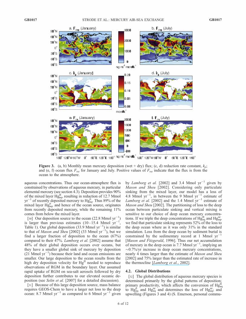
Figure 3. (a, b) Monthly mean mercury deposition (wet + dry) flux; (c, d) reduction rate constant, kp;and (e, f) ocean flux Foa for January and July. Positive values of Foa indicate that the flux is from theocean to the atmosphere.

GB1017 STRODE ET AL.: MERCURY AIR-SEA EXCHANGE

6 of 12

GB1017

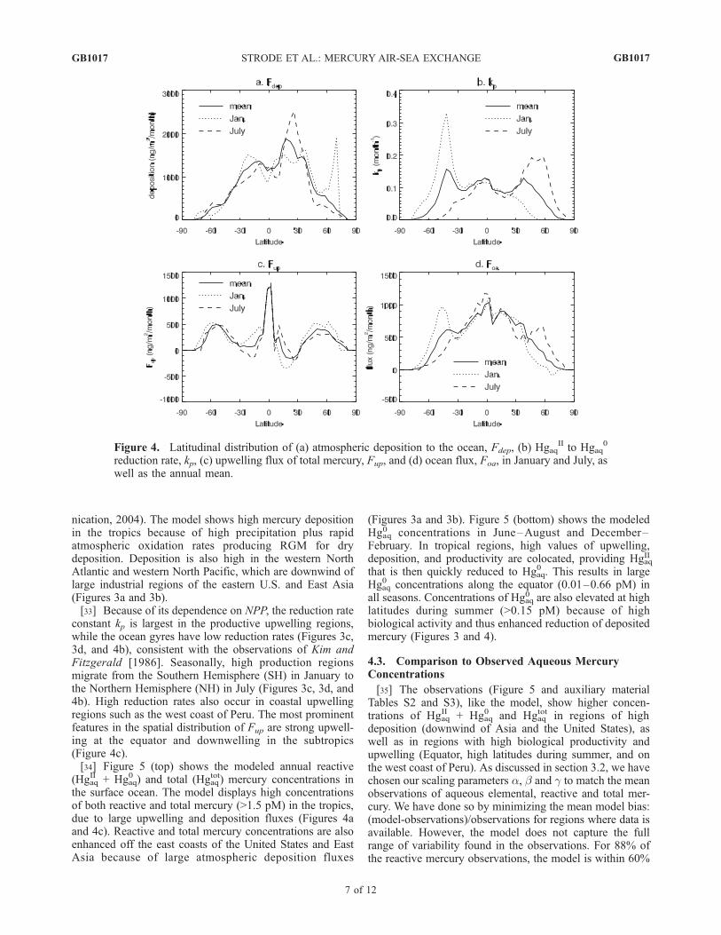
nication, 2004). The model shows high mercury depositionin the tropics because of high precipitation plus rapidatmospheric oxidation rates producing RGM for drydeposition. Deposition is also high in the western NorthAtlantic and western North Pacific, which are downwind oflarge industrial regions of the eastern U.S. and East Asia(Figures 3a and 3b).[33] Because of its dependence on NPP, the reduction rate

constant kp is largest in the productive upwelling regions,while the ocean gyres have low reduction rates (Figures 3c,3d, and 4b), consistent with the observations of Kim andFitzgerald [1986]. Seasonally, high production regionsmigrate from the Southern Hemisphere (SH) in January tothe Northern Hemisphere (NH) in July (Figures 3c, 3d, and4b). High reduction rates also occur in coastal upwellingregions such as the west coast of Peru. The most prominentfeatures in the spatial distribution of Fup are strong upwell-ing at the equator and downwelling in the subtropics(Figure 4c).[34] Figure 5 (top) shows the modeled annual reactive

(HgaqII + Hgaq

0 ) and total (Hgaqtot) mercury concentrations in

the surface ocean. The model displays high concentrationsof both reactive and total mercury (>1.5 pM) in the tropics,due to large upwelling and deposition fluxes (Figures 4aand 4c). Reactive and total mercury concentrations are alsoenhanced off the east coasts of the United States and EastAsia because of large atmospheric deposition fluxes

(Figures 3a and 3b). Figure 5 (bottom) shows the modeledHgaq

0 concentrations in June–August and December–February. In tropical regions, high values of upwelling,deposition, and productivity are colocated, providing Hgaq

II

that is then quickly reduced to Hgaq0 . This results in large

Hgaq0 concentrations along the equator (0.01–0.66 pM) in

all seasons. Concentrations of Hgaq0 are also elevated at high

latitudes during summer (>0.15 pM) because of highbiological activity and thus enhanced reduction of depositedmercury (Figures 3 and 4).

4.3. Comparison to Observed Aqueous MercuryConcentrations

[35] The observations (Figure 5 and auxiliary materialTables S2 and S3), like the model, show higher concen-trations of Hgaq

II + Hgaq0 and Hgaq

tot in regions of highdeposition (downwind of Asia and the United States), aswell as in regions with high biological productivity andupwelling (Equator, high latitudes during summer, and onthe west coast of Peru). As discussed in section 3.2, we havechosen our scaling parameters a, b and g to match the meanobservations of aqueous elemental, reactive and total mer-cury. We have done so by minimizing the mean model bias:(model-observations)/observations for regions where data isavailable. However, the model does not capture the fullrange of variability found in the observations. For 88% ofthe reactive mercury observations, the model is within 60%

Figure 4. Latitudinal distribution of (a) atmospheric deposition to the ocean, Fdep, (b) HgaqII to Hgaq

0

reduction rate, kp, (c) upwelling flux of total mercury, Fup, and (d) ocean flux, Foa, in January and July, aswell as the annual mean.

GB1017 STRODE ET AL.: MERCURY AIR-SEA EXCHANGE

7 of 12

GB1017

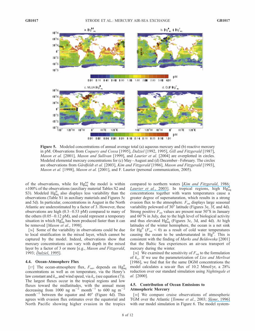
of the observations, while for Hgaqtot the model is within

±100% of the observations (auxiliary material Tables S2 andS3). Modeled Hgaq

0 also displays less variability than theobservations (Table S1 in auxiliary materials and Figures 5cand 5d). In particular, concentrations in August in the NorthAtlantic are underestimated by a factor of 3. However, theseobservations are high (0.3–0.53 pM) compared to many ofthe others (0.05–0.12 pM), and could represent a temporarysituation in which Hgaq

0 has been produced faster than it canbe removed [Mason et al., 1998].[36] Some of the variability in observations could be due

to local stratification in the mixed layer, which cannot becaptured by the model. Indeed, observations show thatmercury concentrations can vary with depth in the mixedlayer by a factor of 3 or more [e.g., Mason and Fitzgerald,1993; Dalziel, 1995].

4.4. Ocean-Atmosphere Flux

[37] The ocean-atmosphere flux, Foa, depends on Hgaq0

concentrations as well as on temperature, via the Henry’slaw constant and kw, and wind speed, via kw (see equation (7)).The largest fluxes occur in the tropical regions and lowfluxes toward the midlatitudes, with the annual meandecreasing from 1000 ng m�2 month�1 to 600 ng m�2

month�1 between the equator and 40� (Figure 4d). Thisagrees with evasion flux estimates over the equatorial andNorth Pacific showing higher evasion in the tropics

compared to northern waters [Kim and Fitzgerald, 1986;Laurier et al., 2003]. In tropical regions, high Hgaq

0

concentrations together with warm temperatures cause agreater degree of supersaturation, which results in a strongevasion flux to the atmosphere. Foa displays large seasonalvariability poleward of 30� latitude (Figures 3e, 3f, and 4d).Strong positive Foa values are present near 50�S in Januaryand 60�N in July, due to the high level of biological activityand thus elevated Hgaq

0 (Figures 3c, 3d, and 4d). At highlatitudes of the winter hemisphere, the ocean is a net sinkfor Hg0 (Foa < 0) as a result of cold water temperaturescausing the ocean to be undersaturated in Hg0. This isconsistent with the finding of Marks and Beldowska [2001]that the Baltic Sea experiences an air-sea transport ofmercury during the winter.[38] We examined the sensitivity of Foa to the formulation

of kw. If we use the parameterization of Liss and Merlivat[1986], we find that for the same DGM concentrations themodel calculates a sea-air flux of 10.2 Mmol/yr, a 28%reduction over our standard simulation using Nightingale etal. [2000].

4.5. Contribution of Ocean Emissions toAtmospheric Mercury

[39] We compare cruise observations of atmosphericTGM over the Atlantic [Temme et al., 2003; Slemr, 1996]with our model simulation in Figure 6. The model system-

Figure 5. Modeled concentrations of annual average total (a) aqueous mercury and (b) reactive mercuryin pM. Observations from Coquery and Cossa [1995], Dalziel [1992, 1995], Gill and Fitzgerald [1987],Mason et al. [2001], Mason and Sullivan [1999], and Laurier et al. [2004] are overplotted in circles.Modeled elemental mercury concentrations for (c) May–August and (d) December–February. The circlesare observations from Gardfeldt et al. [2003], Kim and Fitzgerald [1986], Mason and Fitzgerald [1993],Mason et al. [1998], Mason et al. [2001], and F. Laurier (personal communication, 2005).

GB1017 STRODE ET AL.: MERCURY AIR-SEA EXCHANGE

8 of 12

GB1017

atically underestimates observations in the NH by 25% andhas an interhemispheric gradient of 1.2, smaller than theobserved gradient of 1.5. Selin et al. [2007] demonstratesthat the GEOS-Chem model does reproduce land-basedobservations, which are lower than the ocean cruise obser-vations at the same latitude [Selin et al., 2007, Figure 3].Increasing ocean emissions from 14.1 Mmol yr�1 to21.7 Mmol yr�1 (simulation B) results in better agreementwith the cruise observations in the NH (dashed line inFigure 6), but systematically overestimates SH cruise obser-vations as well as land-based observations (not shown).Thus the magnitude of the ocean emissions cannot resolvethis discrepancy between model and cruise observations.One possibility is that halogen chemistry in the marineboundary layer, which the model neglects, could shift thelatitudinal distribution of deposition to the ocean and henceof the ocean flux. Another possibility is that biomassburning emissions, currently neglected in the model, couldprovide another NH and tropical source.[40] The contribution of ocean emissions to surface at-

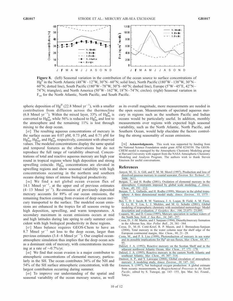
mospheric Hg0 concentrations is shown in Figure 7, whichwas obtained by comparing our standard simulation to asimulation without ocean emissions. In the SH, whereanthropogenic and land sources are relatively small, oceanemissions account for 54% of surface atmospheric mercury,while in the NH, their contribution is 36% on average. Asexpected, the ocean plays a smaller role (<30%) overregions with large anthropogenic sources.[41] The seasonal cycle of regional ocean emissions and

their contribution to surface atmospheric Hg0 concentrationsis shown in Figure 8. Ocean emissions at midlatitudes overthe northern Pacific and Atlantic increase by a factor of 2between winter and spring. This rapid spring increase,which reaches a maximum in May–June, is driven by theincrease in biological productivity and thus large productionof Hgaq

0 via reduction of HgaqII . This is further enhanced by a

decrease in mixed layer depth during that period, leading tothe accumulation of atmospheric deposition in a smallervolume and thus larger Hgaq

0 concentrations.

[42] The maximum effect of ocean emissions on atmo-spheric concentrations occurs in June in the NH andDecember in the SH. The largest seasonal cycles (definedas maximum/minimum) in background Hg0 originatingfrom the ocean are seen over the North pacific (1.32), NorthAtlantic (1.24), and Europe (1.28). This seasonal cycle issmaller over North America (1.21) and the South Pacific(1.15).

5. Summary

[43] We have coupled a global atmospheric model ofmercury transport with an interactive slab model of theocean mixed layer to constrain estimates of ocean emis-sions, simulate their spatiotemporal variability, and examinethe role of the ocean in mercury cycling. We use observa-tions of aqueous elemental (Hgaq

0 ), reactive (Hgaq0 + Hgaq

II ),and total mercury (Hgaq

tot = Hgaq0 +Hgaq

II +Hgaqnr) to constrain

our oceanic simulation.[44] Our modeled mixed layer budget shows mercury

entering the ocean mixed layer primarily through atmo-

Figure 6. Observed atmospheric TGM concentrations over the Atlantic Ocean in (left) 1994 [Slemr,1996] and (right) 1996 [Temme et al., 2003] are shown in black circles. The observations are averaged bymodel grid box, and the error bars represent the standard deviation of the observations within a grid box.Model results sampled along the cruise track for the standard simulation (solid line) and a simulation witha 21.7 Mmol yr�1 ocean flux (simulation B, dashed line) are also shown. The dash-dotted and dottedlines represent the ocean contribution to the surface atmospheric concentration for the standard simulationand simulation B, respectively.

Figure 7. Percent contribution of ocean emissions toatmospheric surface concentrations of Hg0. Contours shownare between 25% and 55%, with increments of 5%.

GB1017 STRODE ET AL.: MERCURY AIR-SEA EXCHANGE

9 of 12

GB1017

spheric deposition of HgII (22.8 Mmol yr�1), with a smallercontribution from diffusion across the thermocline(6.8 Mmol yr�1). Within the mixed layer, 33% of Hgaq

II isconverted to Hgaq

nr, while 56% is reduced to Hgaq0 and lost to

the atmosphere and the remaining 11% is lost throughmixing to the deep ocean.[45] The resulting aqueous concentrations of mercury in

the surface ocean are 0.07 pM, 0.73 pM, and 0.71 pM forHgaq

0 , HgaqII , and Hgaq

nr, respectively, consistent with observedvalues. The modeled concentrations display the same spatialand temporal features as the observations but do notreproduce the full range of variability observed. Concen-trations of total and reactive aqueous mercury are high yearround in tropical regions where high deposition and strongupwelling coincide. Hgaq

0 concentrations are elevated inupwelling regions and show seasonal variability with highconcentrations occurring in the northern and southernoceans during times of intense biological productivity.[46] We find a net global ocean evasion flux of

14.1 Mmol yr�1, at the upper end of previous estimates(4–13 Mmol yr�1). Re-emission of previously depositedmercury accounts for 89% of our ocean emissions, theremaining fraction coming from evasion of deep ocean mer-cury transported to the surface. The modeled ocean emis-sions are enhanced in the tropics for all seasons owing tohigh deposition, upwelling, and warm temperatures. Asecondary maximum in ocean emissions occurs at midand high latitudes during late spring to early summer coin-cident with high biological productivity in these regions.[47] Mass balance requires GEOS-Chem to have an

8.7 Mmol yr�1 net loss to the deep ocean, larger thanprevious estimates (3.4–6 Mmol yr�1). Our coupled ocean-atmosphere simulation thus implies that the deep ocean actsas a dominant sink of mercury, with concentrations increas-ing at a rate of �0.7%/yr.[48] We find that ocean evasion is a major contributor to

atmospheric concentrations of elemental mercury, particu-larly in the SH. The ocean contributes 36% of the NH and54% of the SH surface atmospheric concentration, with thelargest contribution occurring during summer.[49] To improve our understanding of the spatial and

seasonal variability of the ocean mercury source, as well

as its overall magnitude, more measurements are needed inthe open ocean. Measurements of speciated aqueous mer-cury in regions such as the southern Pacific and Indianoceans would be particularly useful. In addition, monthlymeasurements over regions with expected high seasonalvariability, such as the North Atlantic, North Pacific, andSouthern Ocean, would help elucidate the factors control-ling the strong seasonality of ocean emissions.

[50] Acknowledgments. This work was supported by funding fromthe National Science Foundation under grant ATM 0238530. The GEOS-CHEM model is managed by the Atmospheric Chemistry Modeling groupat Harvard University with support from the NASA Atmospheric ChemistryModeling and Analysis Program. The authors wish to thank StevenEmerson for useful conversations.

ReferencesAmyot, M., G. A. Gill, and F. M. M. Morel (1997), Production and loss ofdissolved gaseous mercury in coastal seawater, Environ. Sci. Technol., 31,3606–3611.

Bergan, T., and H. Rodhe (2001), Oxidation of elemental mercury in theatmosphere: Constraints imposed by global scale modeling, J. Atmos.Chem., 40, 191–212.

Bergan, T., L. Gallardo, and H. Rodhe (1999), Mercury in the global tropo-sphere: A three dimensional model study, Atmos. Environ., 33, 1575–1585.

Bey, I., D. J. Jacob, R. M. Yantosca, J. A. Logan, B. Field, A. M. Fiore,Q. Li, H. Y. Liu, L. J. Mickley, and M. G. Schultz (2001), Globalmodeling of tropospheric chemistry with assimilated meteorology: Modeldescription and evaluation, J. Geophys. Res., 106, 23,073–23,095.

Coquery, M., and D. Cossa (1995), Mercury speciation in surface waters ofthe North Sea, Neth. J. Sea Res., 34, 245–257.

Cossa, D., J.-M. Martin, and J. Sanjuan (1994), Dimethylmercury formationin the Alboran Sea, Mar. Pollut. Bull., 28, 381–384.

Cossa, D., M.-H. Cotte-Krief, R. P. Mason, and J. Bretaudeau-Sanjuan(2004), Total mercury in the water column near the shelf edge of theEuropean continental margin, Mar. Chem., 90, 21–29.

Costa, M., and P. S. Liss (1999), Photoreduction of mercury in sea waterand its possible implications for Hg0 air-sea fluxes, Mar. Chem., 68, 87–95.

Dalziel, J. A. (1992), Reactive mercury on the Scotian Shelf and in theadjacent northwest Atlantic Ocean, Mar. Chem., 37, 171–178.

Dalziel, J. A. (1995), Reactive mercury in the eastern North Atlantic andsoutheast Atlantic, Mar. Chem., 49, 307–314.

Dastoor, A. P., and Y. Larocque (2004), Global circulation of atmosphericmercury: A modeling study, Atmos. Environ., 38, 147–161.

Emerson, S. (1997), Net biological oxygen production: A global estimatefrom oceanic measurements, in Biogeochemical Processes in the NorthPacific, edited by S. Tunogai, pp. 143–155, Jpn. Mar. Sci. Found.,Tokyo.

Figure 8. (left) Seasonal variation in the contribution of the ocean source to surface concentrations ofHg0 in the North Atlantic (48�W–12�W, 30�N–60�N; solid line), North Pacific (180�W–138�W, 30�N–60�N; dotted line), South Pacific (180�W–78�W, 30�S–60�N; dashed line), Europe (5�W–45�E, 42�N–74�N; triangles), and North America (50�W–162�W, 18�N–74�N; circles). (right) Seasonal variation inFoa for the North Atlantic, North Pacific, and South Pacific.

GB1017 STRODE ET AL.: MERCURY AIR-SEA EXCHANGE

10 of 12

GB1017

Eppley, R. W., and B. J. Peterson (1979), Particulate organic matter flux andplanktonic new production in the deep ocean, Nature, 282, 677–680.

Esaias, W. E. (1996), Algorithm theoretical basis document for MODISproduct MOD-27 ocean primary productivity, report, NASA GoddardSpace Flight Cent., Greenbelt, Md.

Ferrara, R., C. Ceccarini, E. Lanzillotta, K. Gardfeldt, J. Sommar,M. Horvat, M. Logar, V. Fajon, and J. Kotnik (2003), Profiles of dis-solved gaseous mercury concentration in the Mediterranean seawater,Atmos. Environ., 37, S85–S92.

Fitzgerald, W. F. (1986), Cycling of mercury between the atmosphere andoceans, in Role of Air-Sea Exchange in Geochemical Cycling, NATO ASISer., vol. C185, pp. 363–408, Springer, New York.

Fitzgerald, W. F., D. R. Engstrom, R. P. Mason, and E. A. Nater (1998), Thecase for atmospheric mercury contamination in remote areas, Environ.Sci. Technol., 32, 1–7.

Gardfeldt, K., et al. (2003), Evasion of mercury from coastal and openwaters of the Atlantic Ocean and the Mediterranean Sea, Atmos. Environ.,37, S73–S84.

Gill, G. A., and W. F. Fitzgerald (1987), Mercury in surface waters of theopen ocean, Global Biogeochem. Cycles, 1, 199–212.

Gill, G. A., and W. F. Fitzgerald (1988), Vertical mercury distributions inthe oceans, Geochim. Cosmochim. Acta, 52, 1719–1728.

Guentzel, J. L., R. T. Powell, W. M. Landing, and R. P. Mason (1996),Mercury associated with colloidal material in an estuarine and an open-ocean environment, Mar. Chem., 55, 177–188.

Hall, B. (1995), The gas phase oxidation of elemental mercury by ozone,Water Air Soil Pollut., 80, 301–315.

Hedgecock, I. M., and N. Pirrone (2001), Mercury and photochemistry inthe marine boundary layer-modelling studies suggest the in situ produc-tion of reactive gas phase mercury, Atmos. Environ., 35, 3055–3062.

Hedgecock, I. M., and N. Pirrone (2004), Chasing quicksilver: Modelingthe atmospheric lifetime of Hg(g)

0 in the marine boundary layer at variouslatitudes, Environ. Sci. Technol., 38, 69–76.

Hellerman, S., and M. Rosenstein (1983), Normal monthly wind stress overthe world ocean with error estimates, J. Phys. Oceanogr., 13, 1093–1104.

Horvat, M., J. Kotnik, M. Logar, V. Fajon, T. Zvonaric, and N. Pirrone(2003), Speciation of mercury in surface and deep-sea waters in theMediterranean Sea, Atmos. Environ., 37, S93–S108.

Hudson, R. J. M., S. A. Gherini, W. F. Fitzgerald, and D. B. Porcella(1995), Anthropogenic influences on the global mercury cycle: A model-based approach, Water Air Soil Pollut., 80, 265–272.

Kara, A. B., P. A. Rochford, and H. E. Hurlburt (2003), Mixed layer depthvariability over the global ocean, J. Geophys. Res., 108(C3), 3079,doi:10.1029/2000JC000736.

Kim, J. P., and W. F. Fitzgerald (1986), Sea-air partitioning of mercury inthe equatorial Pacific Ocean, Science, 231, 1131–1133.

Lalonde, J. D., M. Amyot, A. M. L. Kraepiel, and F. M. M. Morel (2001),Photooxidation of Hg(0) in artificial and natural waters, Environ. Sci.Technol., 35, 1367–1372.

Lamborg, C. H., K. R. Rolfhus, W. F. Fitzgerald, and G. Kim (1999), Theatmospheric cycling and air-sea exchange of mercury species in the Southand equatorial Atlantic Ocean, Deep Sea Res., Part II, 46, 957–977.

Lamborg, C. H., W. F. Fitzgerald, J. O’Donnell, and T. Torgersen (2002), Anon-steady-state compartmental model of global-scale mercury biogeo-chemistry with interhemispheric atmospheric gradients, Geochim. Cos-mochim. Acta, 66, 1105–1118.

Lamborg, C. H., C.-M. Tseng, W. F. Fitzgerald, P. H. Balcom, and C. R.Hammerschidt (2003), Determination of the mercury complexation char-acteristics of dissolved organic matter in natural waters with ‘‘ReducibleHg’’ titrations, Environ. Sci. Technol., 37, 3316–3322.

Laurier, F. J. G., R. P. Mason, and L. Whalin (2003), Reactive gaseousmercury formation in the North Pacific Ocean’s marine boundary layer: Apotential role of halogen chemistry, J. Geophys. Res., 108(D17), 4529,doi:10.1029/2003JD003625.

Laurier, F. J. G., R. P. Mason, G. A. Gill, and L. Whalin (2004), Mercurydistributions in the North Pacific Ocean—20 years of observations, Mar.Chem., 90, 3–19.

Laws, W. A., P. G. Falkowski, W. O. Smith Jr., H. Ducklow, and J. J.McCarthy (2000), Temperature effects on export production in the openocean, Global Biogeochem. Cycles, 14, 1231–1246.

Lindqvist, O., K. Johansson, M. Aastrup, A. Andersson, L. Bringmark,G. Hovsenius, L. Hakanson, A. Iverfeldt, M. Meili, and B. Timm(1991), Mercury in the Swedish environment—Recent research on causes,consequences and corrective methods, Water Air Soil Pollut., 55, 11–13.

Liss, P. S., and L. Merlivat (1986), Air-sea gas exchange rates: Introductionand synthesis, in The Role of Air-Sea Exchange in Geochemical Cycling,edited by P. Buat-Menard, pp. 113–127, Springer, New York.

Marks, R., and M. Beldowska (2001), Air-sea exchange of mercury vapourover the Gulf of Gdansk and southern Baltic Sea, J. Mar. Syst., 27, 315–324.

Mason, R. P., and W. F. Fitzgerald (1993), The distribution and biogeo-chemical cycling of mercury in the equatorial Pacific Ocean, Deep SeaRes., Part I, 40, 1897–1924.

Mason, R. P., and W. F. Fitzgerald (1996), Sources, sinks and biogeochem-ical cycling of mercury in the ocean, in Global and Regional MercuryCycles: Sources, Fluxes and Mass Balances, edited by W. Baeyens et al.,pp. 249–272, Elsevier, New York.

Mason, R. P., and G.-R. Sheu (2002), Role of the ocean in the globalmercury cycle, Global Biogeochem. Cycles, 16(4), 1093, doi:10.1029/2001GB001440.

Mason, R. P., and K. A. Sullivan (1999), The distribution and speciation ofmercury in the South and equatorial Atlantic, Deep Sea Res., Part II, 46,937–956.

Mason, R. P., W. F. Fitzgerald, and F. M. M. Morel (1994a), The biogeo-chemical cycling of elemental mercury: Anthropogenic influences, Geo-chim. Cosmochim. Acta, 58, 3191–3198.

Mason, R. P., J. O’Donnell, and W. F. Fitzgerald (1994b), Elemental mer-cury cycling within the mixed layer of the Equatorial Pacific Ocean, inMercury as a Global Pollutant: Towards Integration and Synthesis, edi-ted by C. J. Watras and J. W. Huckabee, pp. 83–97, CRC Press, BocaRaton, Fla.

Mason, R. P., F. M. M. Morel, and H. F. Hemond (1995), The role ofmicroorganisms in elemental mercury formation in natural waters, WaterAir Soil Pollut., 80, 775–787.

Mason, R. P., K. R. Rolfhus, and W. F. Fitzgerald (1998), Mercury in theNorth Atlantic, Mar. Chem., 61, 37–53.

Mason, R. P., N. M. Lawson, and G.-R. Sheu (2001), Mercury in theAtlantic Ocean: Factors controlling air-sea exchange of mercury and itsdistribution in the upper waters, Deep Sea Res., Part II, 48, 2829–2853.

Morel, F. M. M., A. M. L. Krapiel, and M. Amyot (1998), The chemicalcycle and bioaccumulation of mercury, Annu. Rev. Ecol. Syst., 29, 543–566.

National Atmospheric Deposition Program (2003), Mercury DepositionNetwork (MDN): A NADP Network, NADP Program Off., Ill. StateWater Surv., Champaign.

National Research Council (2000), Toxicological Effects of Methylmercury,Natl. Acad., Washington, D. C.

Nightingale, P. D., G. Malin, C. S. Law, A. J. Watson, P. S. Liss, M. I.Liddicoat, J. Boutin, and R. C. Upstill-Goddard (2000), In situ evaluationof air-sea gas exchange parameterizations using novel conservative andvolatile tracers, Global Biogeochem. Cycles, 14, 373–387.

Pacyna, J. M., E. G. Pacyna, F. Steenhuisen, and S. Wilson (2003), Map-ping 1995 global anthropogenic emissions of mercury, Atmos. Environ.,37, S109–S117.

Poissant, L., M. Amyot, M. Pilote, and D. Lean (2000), Mercury water-airexchange over the Upper St. Lawrence River and Lake Ontario, Environ.Sci. Technol., 34, 3069–3078.

Reid, R. C., J. M. Prausnitz, and B. E. Poling (1987), The Properties ofGases and Liquids, McGraw-Hill Inc., New York.

Rolfhus, K. R., and W. F. Fitzgerald (2004), Mechanisms and temporalvariability of dissolved gaseous mercury production in coastal seawater,Mar. Chem., 90, 126–136.

Schroeder, W. H., and J. Munthe (1998), Atmospheric mercury—An over-view, Atmos. Environ., 32, 809–822.

Seigneur, C., P. Karamchandani, K. Lohman, and K. Vijayaraghavan(2001), Multiscale modeling of the atmospheric fate and transport ofmercury, J. Geophys. Res., 106, 27,795–27,809.

Seigneur, C., K. Vijayaraghavan, K. Lohman, P. Karamchandani, andC. Scott (2004), Global source attribution for mercury deposition inthe United States, Environ. Sci. Technol., 38, 555–569.

Selin, N. E., D. J. Jacob, R. J. Park, R. M. Yantosca, S. Strode, L. Jaegle,and D. Jaffe (2007), Chemical cycling and deposition of atmosphericmercury: Global constraints from observations, J. Geophys. Res., 112,D02308, doi:10.1029/2006JD007450.

Shia, R.-L., C. Seigneur, P. Pai, M. Ko, and N. D. Sze (1999), Globalsimulation of atmospheric mercury concentrations and deposition fluxes,J. Geophys. Res., 104, 23,747–23,760.

Slemr, F. (1996), Trends in atmospheric mercury concentrations over theAtlantic Ocean and at the Wank Summit, and the resulting constraints onthe budget of atmospheric mercury, in Global and Regional MercuryCycles: Sources, Fluxes, and Mass Balances, edited by W. Baeyens,R. Ebinghaus, and O. Vasiliev, pp. 33–84, Springer, New York.

Slemr, F., and E. Langer (1992), Increase in global atmospheric concentra-tions of mercury inferred from measurements over the Atlantic Ocean,Nature, 355, 434–437.

GB1017 STRODE ET AL.: MERCURY AIR-SEA EXCHANGE

11 of 12

GB1017

Slemr, F., W. Junkermann, R. W. H. Schmidt, and R. Sladkovic (1995),Indication of change in global and regional trends of atmospheric mer-cury concentrations, Geophys, Res. Lett., 22, 2143–2146.

Slemr, F., E.-G. Brunke, R. Ebinghaus, C. Temme, J. Munthe, I. Wangberg,W. Schroeder, A. Steffen, and T. Berg (2003), Worldwide trend of atmo-spheric mercury since 1997, Geophys. Res. Lett., 30(10), 1516,doi:10.1029/2003GL016954.

Sommar, J., K. Gardfeldt, D. Stromberg, and X. Feng (2001), A kineticstudy of the gas-phase reaction between the hydroxyl radical and atomicmercury, Atmos. Environ., 35, 3049–3054.

Temme, C., F. Slemr, R. Ebinghaus, and J. W. Einax (2003), Distributionof mercury over the Atlantic Ocean in 1996 and 1999–2001, Atmos.Environ., 37, 1889–1897.

Wangberg, I., S. Schmolke, P. Schager, J. Munthe, R. Ebinghaus, andA. Iverfeldt (2001), Estimates of air-sea exchange of mercury in theBaltic Sea, Atmos. Environ., 35, 5477–5485.

Wolfe, M. F., S. Schwarzbach, and R. A. Sulaiman (1998), Effects ofmercury on wildlife: A comprehensive review, Environ. Toxicol. Chem.,17, 146–160.

�������������������������D. J. Jacob, R. J. Park, N. E. Selin, and R. M. Yantosca, Division of

Engineering and Applied Sciences, Harvard University, Cambridge, MA02138, USA.L. Jaegle and S. A. Strode, Department of Atmospheric Sciences,

University of Washington, Box 351640, Seattle, WA 98195-1640, USA.(jaegle@atmos.washington.edu; sstrode@atmos.washington.edu)R. P. Mason, Department of Marine Sciences, University of Connecticut,

Groton, CT 06340, USA.F. Slemr, Air Chemistry Division, Max-Planck-Institute for Chemistry,

Joh.-Joachim-Becher-Weg 27, D-55128, Mainz, Germany.

GB1017 STRODE ET AL.: MERCURY AIR-SEA EXCHANGE

12 of 12

GB1017