
Advanced Planning and Scheduling in Manufacturing and ...
584
Yuri Mauergauz Advanced Planning and Scheduling in Manufacturing and Supply Chains
-
Upload
khangminh22 -
Category
Documents
-
view
0 -
download
0
Transcript of Advanced Planning and Scheduling in Manufacturing and ...

Yuri Mauergauz
Advanced Planning and Scheduling in Manufacturing and Supply Chains
Advanced Planning and Scheduling inManufacturing and Supply Chains

ThiS is a FM Blank Page

Yuri Mauergauz
Advanced Planning andScheduling inManufacturing and SupplyChains

Yuri MauergauzSophus GroupMoscowRussia
ISBN 978-3-319-27521-5 ISBN 978-3-319-27523-9 (eBook)DOI 10.1007/978-3-319-27523-9
Library of Congress Control Number: 2016933485
# Springer International Publishing Switzerland 2012, 2016This work is subject to copyright. All rights are reserved by the Publisher, whether the whole or part ofthe material is concerned, specifically the rights of translation, reprinting, reuse of illustrations,recitation, broadcasting, reproduction on microfilms or in any other physical way, and transmissionor information storage and retrieval, electronic adaptation, computer software, or by similar ordissimilar methodology now known or hereafter developed.The use of general descriptive names, registered names, trademarks, service marks, etc. in thispublication does not imply, even in the absence of a specific statement, that such names are exemptfrom the relevant protective laws and regulations and therefore free for general use.The publisher, the authors and the editors are safe to assume that the advice and information in thisbook are believed to be true and accurate at the date of publication. Neither the publisher nor theauthors or the editors give a warranty, express or implied, with respect to the material containedherein or for any errors or omissions that may have been made.
Printed on acid-free paper
This Springer imprint is published by Springer NatureThe registered company is Springer International Publishing AG Switzerland
Additional material to this book can be downloaded from http://extras.springer.com.

Preface to the English Edition
Despite the relatively large number of books related to production planning
published in English, up to now information constituting the subject of Advanced
Planning and Scheduling has not been gathered together. This situation inspired the
author to present an English translation of his Russian-language book.
This book was conceived as a guide to modern methods of production planning,
based on fairly new scientific achievements and various rules of thumb of practical
planning. Most of the calculation methods are illustrated with numerical examples.
Attached to the English edition is a set of programs for calculating production
schedules and an example of an ERP system operating in the cloud.
The author expresses his profound gratitude to Federica Corradi Dell’Acqua of
Springer publishers. Her systematic support allowed this project to be implemented.
Moscow, Russia Yuri Mauergauz
v

ThiS is a FM Blank Page
Preface to the Russian Edition
At the end of the last century, a large new field of knowledge developed. Nowadays,
it is called “industrial engineering” and is a creative application of the methods and
principles of various scientific disciplines to achieve and maintain a high level of
productivity and profitability in modern industrial enterprises.
The application of industrial engineering is inextricably linked with the use
of quantitative methods using information that circulates in the production system,
and such methods often have complex mathematical justification. Historically,
the concept of industrial engineering started to be used after wide application
of methods known as “operations research”. Another name for these methods is
“management science”, now more commonly called “industrial engineering”.
Since the foundation of industrial engineering is quite sophisticated mathemati-
cal techniques, its application possibilities are determined largely by the available
computing power. Originally, computers were created to solve complex scientific
problems. Subsequently, this equipment started to be used to develop automated
control systems including production management systems.
The introduction of personal computers changed dramatically the possibilities
and the main focus of application of computer technology. The main objective
of computerization in the late twentieth century was automation of accounting
of a variety of resources and operations with them, i.e. information storage. The
automated control systems of enterprises were mainly designed to collect and
integrate data referring to production and sales. Therefore, the development of
industrial engineering at that time was mostly of a scientific and theoretical nature.
In the early twenty-first century, however, the situation changed dramatically.
First of all, against the background of rising resource prices, the issue of production
efficiency is becoming more and more important. In addition, it was found that,
despite their great diversity, the number of accounting problems is limited and most
problems had already been solved, while the increasing capabilities of computer
technology allow more complex problems to be solved. As a result, researchers
and production managers began to turn to the problems of enhancing production
management.
There was a sharp increase in the number of articles in the field of industrial
engineering and a rapid increase in the number of relevant scientific journals.
Today, worldwide, there are at least 30 international English-language journals in
vii
which thousands of scientific articles on industrial engineering are published
annually. In addition, there are a number of national engineering journals, and
in some countries, such as Spain and Iran, they are published with simultaneous
translation into English.
The field of industrial engineering includes management aspects such as the
location of enterprises, determining the range of products, selection of necessary
processes, organization of production divisions, etc. Many of these management
objectives refer to pre-production, but not its realization. The effective implemen-
tation of production is only possible with organized and comprehensive sound
planning, which is actually the final component of industrial engineering.
Until the end of the last century, production planning was mainly based on the
knowledge and experience of the planners themselves who used quite elementary
methods of calculation for different purposes. The use of computer technology, for
the most part, was limited to calculation of the number of products and resources
required.
Due to the complexity of the mathematical description of plans, their optimiza-
tion appeared to be possible after the introduction of powerful personal computers
at the beginning of this century. The relevant methods were used to create a number
of new production control systems, known as APS and MES. In general, the new
planning methods based on complex mathematical models are called Advanced
Planning and Scheduling (AP&S). This book is intended for readers whose
activities are related to production planning, though in different business areas.
First of all, the book is intended as a reference guide for operating production
managers. As the workload of these specialists does not allow them to engage in a
consistent and detailed study of the various methods, the book is designed so that
almost every section, and sometimes even an individual paragraph, can be read
independently of the other sections. At the same time, wherever possible when
describing a method, reference is made to the preceding discussion of the method,
to allow deeper examination of the material.
To make the presentation of each section independent of the previous text,
most of the methods and examples use the same designations of variables and
parameters, and these designations are listed in Appendix A. In those cases where
the designation does not coincide or is not referred to in Appendix A, it is defined in
the text. Each example is accompanied by the method reduced to a final calculation.
The author hopes that this structure will be convenient for developers of production
planning software as well as for production managers.
Not all planning methods described in this book are useful in practice. This
applies to a number of problems and their solutions, which provide a scientific basis
for comparison and a reference sample for other methods, which in turn may be
used in practice.
On the other hand, the book is constructed to provide the opportunity to study
the material consistently. The book is divided into two parts, the first of which
is dedicated to detailed description of models of planning, and the second part
describes the processes carried out on the basis of these models. Some of these
viii Preface to the Russian Edition

models are quite complex, and at first acquaintance their study can be skipped. This
construction is to facilitate learning by researchers, postgraduates, and students.
The challenge in writing this book was the selection of materials and the
sequence of their presentation. An enormous number of different methods of
production planning have been developed. In particular, G. Halevi’s reference
book on production planning methods dated 2001 describes 110 methods, which,
of course, vary to a large extent in the degree of distribution and application. This
book includes those models and planning processes which by the time of writing
were in focus in the scientific literature. It was assumed that production planning
itself is closely connected to the planning of inventory because the result of the
manufacturing process is stock buildup.
The contents of the book, for the most part, are based on the results of scientific
papers contained in a number of English-language guides, monographs, and articles
written at the end of the twentieth and beginning of the twenty-first century. The
author has also tried whenever possible to use the available, albeit few, modern
Russian-language works. Materials relating to the period of development of com-
puter systems in the Soviet Union in the 1970s and 1980s have also been used. The
structure and nature of any presentation always depends largely on the author’s
position. In this case, when considering methods of production planning, special
attention is paid to its regularity and dynamics, i.e. a periodic recurrence and at the
same time the need to introduce various changes, including urgent ones.
Different scientific disciplines are used in themethods of production planning. Each
discipline has its own set of traditional symbols. In this book, itwas important to ensure
consistent use of symbols, so one designation system was chosen as basic. Therefore,
the nomenclature of symbols accepted in scheduling theory is used throughout; in
other cases, some symbols may be different from the conventional ones.
The author is grateful to Professor A.L. Ryzhkowhose comments and suggestions
helped to improve the presentation significantly.
Moscow, Russia Yuri Mauergauz
Preface to the Russian Edition ix

ThiS is a FM Blank Page

Annotation
Advanced Planning and Scheduling (AP&S) in Productionand Supply Chains
The book consists of two parts, the first of which considers construction of refer-
ence and mathematical planning models, production bottleneck models, and multi-
criteria models; examples of such models are provided. The methods of forecasting
and aggregate demand are discussed; background information about the storage and
data processing methods for planning are provided.
The second part analyses various models of stocks planning and the rules for
calculating safety stocks; it also describes the stocks dynamics in the supply chain.
Various methods of batch sizing are detailed. Production planning is studied at
several levels: planning of shipment to customers, calendar scheduling, and opera-
tional planning. Operational planning is considered separately for one-stage and
multi-stage problems as well as for different multi-criteria problems. For some
problems of multi-criteria, scheduling by the methods described in the book special
software is developed.
The book can be used as a reference for modern planning methods as well as a
teaching aid. It is intended for employees of planning and production services,
specialists in enterprise information management systems, and researchers and
graduate students involved in production planning. The book can be used by students
at technical colleges as a guide when writing course papers and graduate theses.
A description of a collection of production schedule programs and an example of
the ERP system operating in the cloud is included in the book.
Moscow, Russia Yuri Mauergauz
xi

ThiS is a FM Blank Page
Contents
Part I Modeling
1 Reference Model . . . . . . . . . . . . . . . . . . . . . . . . . . . . . . . . . . . . . . . 3
1.1 Modelling of Business Process . . . . . . . . . . . . . . . . . . . . . . . . 3
1.2 Concept of Reference Model . . . . . . . . . . . . . . . . . . . . . . . . . . 5
1.2.1 Reference Models in Supply Chains . . . . . . . . . . . . . . 6
1.2.2 Reference Modelling Methodology . . . . . . . . . . . . . . . 7
1.3 Production Description . . . . . . . . . . . . . . . . . . . . . . . . . . . . . . 9
1.3.1 Basic Types of Production . . . . . . . . . . . . . . . . . . . . . 9
1.3.2 Production Scale and Strategy . . . . . . . . . . . . . . . . . . 13
1.4 Advanced Planning in IT Systems . . . . . . . . . . . . . . . . . . . . . . 15
1.4.1 Planning in IT Systems . . . . . . . . . . . . . . . . . . . . . . . 15
1.4.2 Popularity and Effects of Advanced Planning . . . . . . . 19
1.5 IT System Interaction Standards . . . . . . . . . . . . . . . . . . . . . . . 21
1.6 Quality Parameters in Supply Chains . . . . . . . . . . . . . . . . . . . . 24
1.6.1 Markets and Their Main Properties . . . . . . . . . . . . . . . 25
1.6.2 Quality Parameters and Different Supply Chain
Levels . . . . . . . . . . . . . . . . . . . . . . . . . . . . . . . . . . . . 26
1.6.3 Balanced Scorecard . . . . . . . . . . . . . . . . . . . . . . . . . . 28
1.7 Utility of Quality Parameters . . . . . . . . . . . . . . . . . . . . . . . . . . 31
1.7.1 Concept of Utility . . . . . . . . . . . . . . . . . . . . . . . . . . . 31
1.7.2 Typical Utility Functions . . . . . . . . . . . . . . . . . . . . . . 34
1.7.3 Utility Functions in Business Process Quality
Evaluations . . . . . . . . . . . . . . . . . . . . . . . . . . . . . . . . 37
References . . . . . . . . . . . . . . . . . . . . . . . . . . . . . . . . . . . . . . . . . . . . 42
2 Mathematical Models . . . . . . . . . . . . . . . . . . . . . . . . . . . . . . . . . . . 43
2.1 Simplest Planning Models . . . . . . . . . . . . . . . . . . . . . . . . . . . . 43
2.1.1 Classical Supply Management Model . . . . . . . . . . . . . 43
2.1.2 Continuous Linear Optimization Model . . . . . . . . . . . . 45
2.2 Correlations Between Mathematical and Reference Models . . . . 52
2.2.1 Main Criteria and Constraints . . . . . . . . . . . . . . . . . . . 52
2.2.2 Standard Classification of Planning Optimization
Models . . . . . . . . . . . . . . . . . . . . . . . . . . . . . . . . . . . 53
xiii
2.2.3 Production Scale and Plan Hierarchy in Classification . . . 55
2.3 Priority Rules . . . . . . . . . . . . . . . . . . . . . . . . . . . . . . . . . . . . . 58
2.3.1 Simple Rules . . . . . . . . . . . . . . . . . . . . . . . . . . . . . . . 58
2.3.2 Some Useful Theorems . . . . . . . . . . . . . . . . . . . . . . . 62
2.3.3 Combined Priority Rules . . . . . . . . . . . . . . . . . . . . . . 62
2.4 Production Intensity and Utility of Orders . . . . . . . . . . . . . . . . 64
2.4.1 Production Intensity . . . . . . . . . . . . . . . . . . . . . . . . . . 65
2.4.2 Dynamic Utility Function of Orders . . . . . . . . . . . . . . 70
2.5 More Complex Models of Linear Optimization . . . . . . . . . . . . 74
2.5.1 Integer Linear Optimization Model . . . . . . . . . . . . . . . 74
2.5.2 Integer Linear Optimization Models with Binary
Variables . . . . . . . . . . . . . . . . . . . . . . . . . . . . . . . . . . 75
2.6 Fixed Job Sequence Models . . . . . . . . . . . . . . . . . . . . . . . . . . 78
2.6.1 Branch-and-Bound Method with Minimum Cumulative
Tardiness Tw . . . . . . . . . . . . . . . . . . . . . . . . . . . . . . . 79
2.6.2 Branch-and-Bound Method with Maximum Average
Utility V . . . . . . . . . . . . . . . . . . . . . . . . . . . . . . . . . . 81
References . . . . . . . . . . . . . . . . . . . . . . . . . . . . . . . . . . . . . . . . . . . . 87
3 Production Bottlenecks Models . . . . . . . . . . . . . . . . . . . . . . . . . . . . 89
3.1 Theory of Constraints . . . . . . . . . . . . . . . . . . . . . . . . . . . . . . . 89
3.1.1 Fundamentals of Theory of Constraints . . . . . . . . . . . . 89
3.1.2 Bottleneck Operation Planning . . . . . . . . . . . . . . . . . . 92
3.1.3 Planning for Buffers, Ropes, and Non-bottleneck
Machines . . . . . . . . . . . . . . . . . . . . . . . . . . . . . . . . . . 95
3.1.4 Simple Example of Theory of Constraints
in Application . . . . . . . . . . . . . . . . . . . . . . . . . . . . . . 97
3.1.5 Theory of Constraints in Process Manufacturing . . . . . 98
3.1.6 Review of TOC Applications . . . . . . . . . . . . . . . . . . . 100
3.2 Theory of Logistic Operating Curves . . . . . . . . . . . . . . . . . . . . 101
3.2.1 Production (Logistics) Variables . . . . . . . . . . . . . . . . . 101
3.2.2 Some Notions Used in Queuing Theory . . . . . . . . . . . . 105
3.2.3 Plotting Logistic Operating Curves . . . . . . . . . . . . . . . 107
3.2.4 Main Properties of Logistic Curves . . . . . . . . . . . . . . . 110
3.3 Application of Logistic Operating Curves . . . . . . . . . . . . . . . . 110
3.3.1 Logistic Positioning . . . . . . . . . . . . . . . . . . . . . . . . . . 110
3.3.2 Bottleneck Analysis and Improvements . . . . . . . . . . . . 111
3.3.3 Evaluation of Overall Production Performance . . . . . . 112
3.4 Optimal Lot Sizing for Production Bottlenecks . . . . . . . . . . . . . 116
3.4.1 Lot Sizing Heuristic . . . . . . . . . . . . . . . . . . . . . . . . . . 116
3.4.2 Analysis of Heuristic Solutions . . . . . . . . . . . . . . . . . . 119
3.5 Hierarchical Approach to Machinery Load Management . . . . . . 122
3.5.1 Principles of Workload Control Concept . . . . . . . . . . . 123
3.5.2 Example of Application of Controlled Load Approach . . . 124
References . . . . . . . . . . . . . . . . . . . . . . . . . . . . . . . . . . . . . . . . . . . . 126
xiv Contents
4 Multi-criteria Models and Decision-Making . . . . . . . . . . . . . . . . . . 127
4.1 Basic Concepts in Multi-criteria Optimization Theory . . . . . . . 127
4.1.1 Definition of Multi-criteria Optimization Problems . . . 127
4.1.2 Pareto Optimality . . . . . . . . . . . . . . . . . . . . . . . . . . . . 130
4.1.3 Main Methods of Solving Multi-criteria Planning
Problems . . . . . . . . . . . . . . . . . . . . . . . . . . . . . . . . . . 132
4.1.4 Analytical Method of Constructing a Trade-Off Curve . . . 136
4.2 Optimized Multi-criteria Lot Sizing . . . . . . . . . . . . . . . . . . . . . 138
4.2.1 Lot Sizing Based on Costs and Equipment . . . . . . . . . 138
4.2.2 Analytical Lot Sizing with Two Criteria: Setup Time
and Cost . . . . . . . . . . . . . . . . . . . . . . . . . . . . . . . . . . 140
4.3 Example of Multi-scheduling Problem . . . . . . . . . . . . . . . . . . . 143
4.3.1 Special ε-Neighbourhood of Efficiency Points . . . . . . . 144
4.3.2 Solving Algorithm . . . . . . . . . . . . . . . . . . . . . . . . . . . 145
4.4 Methods of Decision-Making Theory in Planning Problems . . . 150
4.4.1 Some Information from the Decision Making Theory . . . 150
4.4.2 Example of the Planning Problem Requiring Decision
Making . . . . . . . . . . . . . . . . . . . . . . . . . . . . . . . . . . . 153
4.4.3 Decision-Making Based on the Guaranteed Result
Principle . . . . . . . . . . . . . . . . . . . . . . . . . . . . . . . . . . 156
4.4.4 Optimistic Decision-Making . . . . . . . . . . . . . . . . . . . . 157
4.5 Applications of Complex Decision-Making Methods . . . . . . . . 158
4.5.1 Hurwitz Principle . . . . . . . . . . . . . . . . . . . . . . . . . . . . 158
4.5.2 Savage Principle . . . . . . . . . . . . . . . . . . . . . . . . . . . . 159
4.5.3 Shifted Ideal Method . . . . . . . . . . . . . . . . . . . . . . . . . 160
References . . . . . . . . . . . . . . . . . . . . . . . . . . . . . . . . . . . . . . . . . . . . 162
5 Data for Planning . . . . . . . . . . . . . . . . . . . . . . . . . . . . . . . . . . . . . . 163
5.1 Composition of the Data Used for Planning . . . . . . . . . . . . . . . 163
5.1.1 Archives of Design-Engineering Documentation and
Orders . . . . . . . . . . . . . . . . . . . . . . . . . . . . . . . . . . . . 163
5.1.2 Reference Data and Standards . . . . . . . . . . . . . . . . . . 167
5.1.3 Databases of Transactional IT Systems . . . . . . . . . . . . 169
5.1.4 Decision Support Databases . . . . . . . . . . . . . . . . . . . . 170
5.1.5 Knowledge Bases . . . . . . . . . . . . . . . . . . . . . . . . . . . . 171
5.2 Data Storage and Management . . . . . . . . . . . . . . . . . . . . . . . . 174
5.2.1 Relational Databases . . . . . . . . . . . . . . . . . . . . . . . . . 174
5.2.2 Concept of Object-Oriented Databases . . . . . . . . . . . . 176
5.2.3 Database Management Systems . . . . . . . . . . . . . . . . . 177
5.2.4 Tiered Data Storage . . . . . . . . . . . . . . . . . . . . . . . . . . 178
5.2.5 Distributed Databases . . . . . . . . . . . . . . . . . . . . . . . . . 179
5.2.6 Service Oriented Architecture of IT Systems . . . . . . . . 181
5.2.7 On-Line Analytical Processing . . . . . . . . . . . . . . . . . . 183
5.3 Information Exchange . . . . . . . . . . . . . . . . . . . . . . . . . . . . . . . 186
Contents xv
5.3.1 Internal Data Communication . . . . . . . . . . . . . . . . . . . 186
5.3.2 Data Transfer Between Enterprises . . . . . . . . . . . . . . . 187
5.3.3 Information Exchange in Different Types of
Cooperation . . . . . . . . . . . . . . . . . . . . . . . . . . . . . . . . 189
5.3.4 Information Exchange Automation . . . . . . . . . . . . . . . 191
5.3.5 Use of Cloud Environment . . . . . . . . . . . . . . . . . . . . . 194
References . . . . . . . . . . . . . . . . . . . . . . . . . . . . . . . . . . . . . . . . . . . . 196
6 Demand Forecasting . . . . . . . . . . . . . . . . . . . . . . . . . . . . . . . . . . . . 199
6.1 Demand Modelling Based on Time Series Analysis . . . . . . . . . 199
6.2 Main Methods of Forecasting . . . . . . . . . . . . . . . . . . . . . . . . . 201
6.2.1 Moving Average Method . . . . . . . . . . . . . . . . . . . . . . 201
6.2.2 Exponentially Smoothing Forecasting . . . . . . . . . . . . . 203
6.2.3 Trend Adjusted Exponential Smoothing . . . . . . . . . . . 204
6.2.4 Trend and Seasonality Adjusted Exponential
Smoothing . . . . . . . . . . . . . . . . . . . . . . . . . . . . . . . . . 206
6.3 Demand Aggregation . . . . . . . . . . . . . . . . . . . . . . . . . . . . . . . 208
6.4 Aggregated Demand Forecasting . . . . . . . . . . . . . . . . . . . . . . . 210
References . . . . . . . . . . . . . . . . . . . . . . . . . . . . . . . . . . . . . . . . . . . . 214
7 Examples of Advanced Planning Models . . . . . . . . . . . . . . . . . . . . . 215
7.1 Joint Operation Model of APS System and ERP System
from SAP R/3 . . . . . . . . . . . . . . . . . . . . . . . . . . . . . . . . . . . . . 215
7.1.1 Main Business Process Attributes in Various
Industries . . . . . . . . . . . . . . . . . . . . . . . . . . . . . . . . . . 216
7.1.2 Software Modules for Planning Solutions . . . . . . . . . . 218
7.1.3 Planning Modules Interaction . . . . . . . . . . . . . . . . . . . 219
7.2 Reference Model of Production Planning for Instrument
Engineering Plant . . . . . . . . . . . . . . . . . . . . . . . . . . . . . . . . . . 221
7.2.1 Initial Planning Status Analysis . . . . . . . . . . . . . . . . . 221
7.2.2 Decision Support Database . . . . . . . . . . . . . . . . . . . . . 223
7.3 Mathematical Model in Chemical Industry . . . . . . . . . . . . . . . . 226
7.3.1 Analytical Structure of Model . . . . . . . . . . . . . . . . . . . 226
7.3.2 Objective Function and Constraints . . . . . . . . . . . . . . . 229
7.3.3 Some Results of Modelling . . . . . . . . . . . . . . . . . . . . . 233
7.4 Rapid Supply Chain Reference Model in Clothing Industry . . . . 234
7.5 Schedule Model for a Machine Shop . . . . . . . . . . . . . . . . . . . . 237
7.5.1 Schedule Model with Specified Processing Stages . . . . 238
7.5.2 Optimality Criteria and Constraints . . . . . . . . . . . . . . . 239
7.6 Multi-stage Logistics Chain Model . . . . . . . . . . . . . . . . . . . . . 241
7.6.1 Some Notions in Logistics Chain Modelling . . . . . . . . 241
7.6.2 Dynamic Logistics Chain Optimization Model
in Multi-stage Production . . . . . . . . . . . . . . . . . . . . . . 241
References . . . . . . . . . . . . . . . . . . . . . . . . . . . . . . . . . . . . . . . . . . . . 244
xvi Contents
Part II Planning Processes
8 Single-Echelon Inventory Planning . . . . . . . . . . . . . . . . . . . . . . . . . 247
8.1 Inventory Types and Parameters . . . . . . . . . . . . . . . . . . . . . . . 247
8.2 Inventory Management Models . . . . . . . . . . . . . . . . . . . . . . . . 248
8.2.1 Model with Fixed Quantity of Order . . . . . . . . . . . . . . 249
8.2.2 Model with Fixed Reorder Cycle . . . . . . . . . . . . . . . . 250
8.2.3 Two-Tier Inventory Management Model . . . . . . . . . . . 251
8.2.4 Benchmarking of Inventory Management Models . . . . 253
8.2.5 Kanban Inventory Management Model . . . . . . . . . . . . 254
8.3 Inventory Management Model Under Uncertainty . . . . . . . . . . 256
8.3.1 Customer Service Level . . . . . . . . . . . . . . . . . . . . . . . 256
8.3.2 Shortages Permitted Inventory Management Model . . . 257
8.3.3 Demand Distribution Functions . . . . . . . . . . . . . . . . . 258
8.3.4 Newsvendor Problem . . . . . . . . . . . . . . . . . . . . . . . . . 260
8.4 Inventory Management Using Logistic Operating Curves . . . . . 262
8.4.1 Storage Curves and Their Applications . . . . . . . . . . . . 262
8.4.2 Finished Product Inventory Sizing to Optimize the
Overall Production Performance . . . . . . . . . . . . . . . . . 264
8.5 Safety Stock Sizing . . . . . . . . . . . . . . . . . . . . . . . . . . . . . . . . . 265
8.5.1 Calculation of Safety Stock with Random Demand . . . 266
8.5.2 Sizing of Safety Stock with Two Random Variables . . . 267
8.5.3 Sizing of Safety Stock with Three Random Variables . . . 269
References . . . . . . . . . . . . . . . . . . . . . . . . . . . . . . . . . . . . . . . . . . . . 270
9 Supply Chain Inventory Dynamics . . . . . . . . . . . . . . . . . . . . . . . . . 273
9.1 Stock Distribution Planning in the Chain . . . . . . . . . . . . . . . . . 273
9.1.1 DRP Technique . . . . . . . . . . . . . . . . . . . . . . . . . . . . . 273
9.1.2 Regular Maintenance of DRP Tables . . . . . . . . . . . . . . 276
9.1.3 Parallel Multi-product Planning . . . . . . . . . . . . . . . . . 278
9.1.4 Inventory Dynamics at Long Lead Cycles . . . . . . . . . . 279
9.2 Supply Chain Fluctuations . . . . . . . . . . . . . . . . . . . . . . . . . . . . 281
9.2.1 Bullwhip Effect . . . . . . . . . . . . . . . . . . . . . . . . . . . . . 281
9.2.2 Bullwhip Effect Factors . . . . . . . . . . . . . . . . . . . . . . . 284
9.2.3 Methods of Reducing Supply Chain Fluctuations . . . . . 286
9.3 Application of Logistics Operating Curves in Supply Chains . . . 289
9.4 Inventory Echelon Accounting . . . . . . . . . . . . . . . . . . . . . . . . 292
9.4.1 Inventory Echeloning . . . . . . . . . . . . . . . . . . . . . . . . . 292
9.4.2 Sequential Supply Chain . . . . . . . . . . . . . . . . . . . . . . 293
9.4.3 Supply Chain with Distribution . . . . . . . . . . . . . . . . . . 297
9.4.4 Dependency Between Echelon Stock and Number
of Links of One Level in the Supply Chain . . . . . . . . . 299
9.5 Inventory Planning in Spare Parts Supply Chains . . . . . . . . . . . 300
9.5.1 METRIC Method in Spare Parts Supplies . . . . . . . . . . 301
Contents xvii
9.5.2 Inventory Planning for Central Spare Parts Storage Using
(R,Q) Model . . . . . . . . . . . . . . . . . . . . . . . . . . . . . . . 305
9.6 Coordinated Planning Between Two Supply Chain
Members . . . . . . . . . . . . . . . . . . . . . . . . . . . . . . . . . . . . . . . . 308
References . . . . . . . . . . . . . . . . . . . . . . . . . . . . . . . . . . . . . . . . . . . . 311
10 Planning of Supplies to Consumers . . . . . . . . . . . . . . . . . . . . . . . . . 313
10.1 Sales and Operation Planning . . . . . . . . . . . . . . . . . . . . . . . . . 313
10.1.1 Interrelation Between Various Planning Directions with
Sales and Operations Plan . . . . . . . . . . . . . . . . . . . . . 313
10.1.2 Sales and Operation Planning Methods . . . . . . . . . . . . 315
10.2 Sales and Operation Plan Optimization Using Linear
Programming . . . . . . . . . . . . . . . . . . . . . . . . . . . . . . . . . . . . . 318
10.2.1 Single Aggregated Product Group Optimization . . . . . . 319
10.2.2 More Complex Case of Optimization of Sales and
Operations Plan . . . . . . . . . . . . . . . . . . . . . . . . . . . . . 322
10.3 Customized Reservation of Products . . . . . . . . . . . . . . . . . . . . 326
10.3.1 Business Process of Response to New Orders . . . . . . . 326
10.3.2 Arrangement of Orders . . . . . . . . . . . . . . . . . . . . . . . . 327
10.3.3 Running ATP Process . . . . . . . . . . . . . . . . . . . . . . . . 329
10.4 Agreement of Order Specifications with Customers . . . . . . . . . 331
10.4.1 Problem Criteria and Their Evaluation . . . . . . . . . . . . 331
10.4.2 Selection of Ordered Product Analogues . . . . . . . . . . . 332
References . . . . . . . . . . . . . . . . . . . . . . . . . . . . . . . . . . . . . . . . . . . . 338
11 Lot Sizing . . . . . . . . . . . . . . . . . . . . . . . . . . . . . . . . . . . . . . . . . . . . 339
11.1 Classification of Lot-Sizing Problems . . . . . . . . . . . . . . . . . . . 339
11.1.1 Lot Properties and Main Problems . . . . . . . . . . . . . . . 339
11.1.2 Lot-Sizing Problems with No Capacity Limits . . . . . . . 341
11.1.3 Lot-Sizing Problems with Limited Capacities and Large
Planning Periods . . . . . . . . . . . . . . . . . . . . . . . . . . . . 342
11.1.4 Lot-Sizing Problems with Limited Capacities and Small
Planning Periods . . . . . . . . . . . . . . . . . . . . . . . . . . . . 343
11.2 Constant Demand Lot-Sizing Problems . . . . . . . . . . . . . . . . . . 344
11.2.1 Models with Gradual Inventory Replenishment . . . . . . 345
11.2.2 Model Applicable to the Machinery Industry If No Cost
Information Is Available . . . . . . . . . . . . . . . . . . . . . . . 347
11.2.3 Three-Parameter Models for Machinery Industry . . . . . 349
11.2.4 Lot Sizing at Discounted Prices . . . . . . . . . . . . . . . . . 351
11.3 Lot Sizing at Variable Demand and Limited Planning
Horizon . . . . . . . . . . . . . . . . . . . . . . . . . . . . . . . . . . . . . . . . . 352
11.3.1 Exact Solution . . . . . . . . . . . . . . . . . . . . . . . . . . . . . . 353
11.3.2 Heuristic Silver–Meal Algorithm . . . . . . . . . . . . . . . . 356
11.3.3 Part Period Balancing . . . . . . . . . . . . . . . . . . . . . . . . . 359
11.3.4 Groff’s Heuristic Rule . . . . . . . . . . . . . . . . . . . . . . . . 360
xviii Contents
11.3.5 Period Order Quantity . . . . . . . . . . . . . . . . . . . . . . . . 362
11.4 Lot Sizing with Constraints . . . . . . . . . . . . . . . . . . . . . . . . . . . 363
11.5 Multi-product Deliveries and Orders . . . . . . . . . . . . . . . . . . . . 366
11.5.1 Optimal Multi-product Lot Sizing . . . . . . . . . . . . . . . . 366
11.5.2 Multi-product Deliveries over Multiple Periods . . . . . . 368
11.5.3 Power-of-Two Policies for Multi-product
Deliveries . . . . . . . . . . . . . . . . . . . . . . . . . . . . . . . . . 370
References . . . . . . . . . . . . . . . . . . . . . . . . . . . . . . . . . . . . . . . . . . . . 371
12 Production Planning . . . . . . . . . . . . . . . . . . . . . . . . . . . . . . . . . . . . 373
12.1 Master Production Planning . . . . . . . . . . . . . . . . . . . . . . . . . . 373
12.1.1 Master Planning as Product Tables . . . . . . . . . . . . . . . 374
12.1.2 Group Master Planning . . . . . . . . . . . . . . . . . . . . . . . 379
12.1.3 Master Production Plan Optimization . . . . . . . . . . . . . 381
12.2 Material Requirement Planning . . . . . . . . . . . . . . . . . . . . . . . . 383
12.2.1 Production Lot Duration . . . . . . . . . . . . . . . . . . . . . . . 384
12.2.2 Optimal Production Lot Sizing . . . . . . . . . . . . . . . . . . 386
12.2.3 Analysis of the Material Requirement Plan . . . . . . . . . 390
12.3 Project-Based Planning . . . . . . . . . . . . . . . . . . . . . . . . . . . . . . 391
12.3.1 Critical Path Method . . . . . . . . . . . . . . . . . . . . . . . . . 391
12.3.2 Cost Optimization at Various Project Stages . . . . . . . . 394
12.4 Stability of Planning . . . . . . . . . . . . . . . . . . . . . . . . . . . . . . . . 398
12.4.1 Quantitative Evaluation of Planning Stability . . . . . . . 399
12.4.2 Methods of Planning Stability Improvement . . . . . . . . 401
References . . . . . . . . . . . . . . . . . . . . . . . . . . . . . . . . . . . . . . . . . . . . 404
13 Shop Floor Scheduling: Single-Stage Problems . . . . . . . . . . . . . . . . 405
13.1 Single-Machine Scheduling with Minimized Overdue
Penalties . . . . . . . . . . . . . . . . . . . . . . . . . . . . . . . . . . . . . . . . 405
13.1.1 Schedule with the Minimum of Delayed Jobs . . . . . . . 406
13.1.2 Scheduling with Minimum Weighted Tardiness
per Each Job . . . . . . . . . . . . . . . . . . . . . . . . . . . . . . . 406
13.1.3 Schedule Optimization with Earliness/Tardiness . . . . . 409
13.2 Common Shipment Date Scheduling . . . . . . . . . . . . . . . . . . . . 410
13.2.1 Fixed Date Schedule Optimization . . . . . . . . . . . . . . . 410
13.2.2 More Complex Cases of Scheduling with Fixed Date . . . 412
13.2.3 Selection of Optimal Midpoint Date for Shipping . . . . 413
13.3 Some Other Scheduling Problems for Jobs with Fixed
Processing Time . . . . . . . . . . . . . . . . . . . . . . . . . . . . . . . . . . . 415
13.3.1 Schedules for the Case of Several Jobs, the Part of
Which Has the Preset Sequence . . . . . . . . . . . . . . . . . 415
13.3.2 Scheduling of Jobs with Different Arrival Time . . . . . . 417
13.3.3 Scheduling of Jobs with Different Arrival Time and
Different Shipment Time . . . . . . . . . . . . . . . . . . . . . . 418
13.3.4 Job Sequence-Based Setup Time Scheduling . . . . . . . . 419
Contents xix
13.4 Periodic Scheduling with Lots of Economic Sizes . . . . . . . . . . 421
13.4.1 Equal-Time Schedules for All Products . . . . . . . . . . . . 421
13.4.2 Variable-Time Schedules for Different Products . . . . . 423
13.5 Group Technology in Schedules for a Single Machine . . . . . . . 426
13.5.1 Group Scheduling for Series Batches . . . . . . . . . . . . . 427
13.5.2 Group Scheduling for Parallel Batches with Minimum
Tardiness Criterion . . . . . . . . . . . . . . . . . . . . . . . . . . 430
13.5.3 Group Scheduling for Parallel Batches with Maximum
Average Utility Criterion . . . . . . . . . . . . . . . . . . . . . . 432
13.6 Parallel Machine Scheduling . . . . . . . . . . . . . . . . . . . . . . . . . . 440
13.6.1 Identical Parallel Machine Scheduling . . . . . . . . . . . . . 440
13.6.2 Schedules for Parallel Unrelated Machines . . . . . . . . . 442
References . . . . . . . . . . . . . . . . . . . . . . . . . . . . . . . . . . . . . . . . . . . . 445
14 Shop Floor Scheduling: Multi-stage Problems . . . . . . . . . . . . . . . . 447
14.1 Synchronized Flowshop Production . . . . . . . . . . . . . . . . . . . . . 447
14.1.1 Discrete Product Lines . . . . . . . . . . . . . . . . . . . . . . . . 448
14.1.2 Lines for Process Production . . . . . . . . . . . . . . . . . . . 449
14.1.3 Flexible Flow Lines . . . . . . . . . . . . . . . . . . . . . . . . . . 450
14.2 Automated Assembly Lines . . . . . . . . . . . . . . . . . . . . . . . . . . . 452
14.2.1 Scheduling for Unpaced Assembly Lines . . . . . . . . . . 453
14.2.2 Scheduling for Paced Assembly Line . . . . . . . . . . . . . 456
14.2.3 Scheduling for Mixed Assembly Lines . . . . . . . . . . . . 460
14.3 Unsynchronized Flowshop Production . . . . . . . . . . . . . . . . . . . 462
14.3.1 Modelling for Unsynchronized (Discontinuous)
Flow Lines . . . . . . . . . . . . . . . . . . . . . . . . . . . . . . . . 463
14.3.2 Optimization for Two-Machine Group Flow Lines . . . . 466
14.3.3 Campbell, Dudek, and Smith Algorithm . . . . . . . . . . . 468
14.3.4 Nawaz, Enscore, Ham Algorithm . . . . . . . . . . . . . . . . 469
14.4 Job-Shop Production . . . . . . . . . . . . . . . . . . . . . . . . . . . . . . . . 470
14.4.1 Shifting Bottleneck Algorithm . . . . . . . . . . . . . . . . . . 471
14.4.2 Job-Shop Production Scheduling Using Dynamic List
Algorithms . . . . . . . . . . . . . . . . . . . . . . . . . . . . . . . . 476
References . . . . . . . . . . . . . . . . . . . . . . . . . . . . . . . . . . . . . . . . . . . . 483
15 Multi-criteria Scheduling . . . . . . . . . . . . . . . . . . . . . . . . . . . . . . . . 485
15.1 Just-in-Time Production Scheduling . . . . . . . . . . . . . . . . . . . . . 485
15.1.1 Starting Group of Jobs with Fixed Sequence . . . . . . . . 485
15.1.2 Scheduling for Identical Parallel Machines with
Common Shipment Date . . . . . . . . . . . . . . . . . . . . . . 489
15.2 Multi-objective Algorithms for Some Simple Production
Structures . . . . . . . . . . . . . . . . . . . . . . . . . . . . . . . . . . . . . . . . 490
15.2.1 Scheduling for Two-Machine Flowshop Production . . . 490
15.2.2 Schedule for Parallel Uniform Machines . . . . . . . . . . . 493
15.2.3 Some Other Problems and Solving Challenges . . . . . . . 499
xx Contents
15.3 Scheduling Based on Cost and Average Orders Utility . . . . . . . 501
15.3.1 Sequenced Job Scheduling with Sequence-Dependent
Setups . . . . . . . . . . . . . . . . . . . . . . . . . . . . . . . . . . . . 502
15.3.2 Group Scheduling for Parallel Batches Based on
Maximum Average Utility and Minimum
Setup Costs . . . . . . . . . . . . . . . . . . . . . . . . . . . . . . . . 511
15.4 Application of Decision Theory Methods . . . . . . . . . . . . . . . . . 515
15.4.1 Application of Savage Principle for
Decision-Making . . . . . . . . . . . . . . . . . . . . . . . . . . . . 516
15.4.2 Application of Hurwitz Principle for
Decision-Making . . . . . . . . . . . . . . . . . . . . . . . . . . . . 518
15.5 Decision-Support Systems . . . . . . . . . . . . . . . . . . . . . . . . . . . . 519
15.5.1 Decision-Support System for Hybrid Flow Lines . . . . . 519
15.5.2 Some Other Decision-Support Systems . . . . . . . . . . . . 521
References . . . . . . . . . . . . . . . . . . . . . . . . . . . . . . . . . . . . . . . . . . . . 523
Appendix A: Symbols . . . . . . . . . . . . . . . . . . . . . . . . . . . . . . . . . . . . . . . 525
Appendix B: Abbreviations . . . . . . . . . . . . . . . . . . . . . . . . . . . . . . . . . . 527
Appendix C: Classification Parameters of Schedules . . . . . . . . . . . . . . . 529
C.1 Parameters in Field α . . . . . . . . . . . . . . . . . . . . . . . . . . . . . . . . . . 529
C.2 Parameters in Field β . . . . . . . . . . . . . . . . . . . . . . . . . . . . . . . . . . 530
C.3 Parameters in Field γ . . . . . . . . . . . . . . . . . . . . . . . . . . . . . . . . . . 530
Appendix D: Production Intensity Integral Calculations . . . . . . . . . . . . 533
Appendix E: Scheduling Software Based on Order Utility Functions . . . 537
E.1 General . . . . . . . . . . . . . . . . . . . . . . . . . . . . . . . . . . . . . . . . . . . . 537
E.2 Description of Work with File1.xls . . . . . . . . . . . . . . . . . . . . . . . . 537
E.3 Description of Work with File2.xls . . . . . . . . . . . . . . . . . . . . . . . . 543
E.4 Description of Work with File3.xls . . . . . . . . . . . . . . . . . . . . . . . . 545
E.5 Description of Work with File4.xls . . . . . . . . . . . . . . . . . . . . . . . . 548
E.6 Description of Work with File5.xls . . . . . . . . . . . . . . . . . . . . . . . . 550
E.7 Description of Work with File6.xls . . . . . . . . . . . . . . . . . . . . . . . . 553
E.8 Description of Work with File7.xls . . . . . . . . . . . . . . . . . . . . . . . . 556
E.9 Description of Work with File8.xls . . . . . . . . . . . . . . . . . . . . . . . . 557
Appendix F: Using Clobbi . . . . . . . . . . . . . . . . . . . . . . . . . . . . . . . . . . . 561
F.1 General . . . . . . . . . . . . . . . . . . . . . . . . . . . . . . . . . . . . . . . . . . . . 561
F.2 Description of Planning Possibilities in the System . . . . . . . . . . . . . 563
F.3 Description of Service Operation . . . . . . . . . . . . . . . . . . . . . . . . . . 564
F.4 Clobbi Service Advantages . . . . . . . . . . . . . . . . . . . . . . . . . . . . . . 566
F.5 Online Registration of Manufacturing Events . . . . . . . . . . . . . . . . . 568
F.6 Clobbi Commercial Use . . . . . . . . . . . . . . . . . . . . . . . . . . . . . . . . 569
Contents xxi

ThiS is a FM Blank Page

About the Author
Yuri Mauergauz is an Assistant Professor and a consultant of Sophus Group,
Moscow, Russia. He gained his PhD from the St. Petersburg Navy Institute in
1970. He has worked at machine-building plants and research institutes and also
taught at the Urals and Odessa technical universities. He has published around
80 research papers and 3 books dedicated to the application of computer engineering
in production planning.
xxiii

Part I
Modeling

Reference Model 1
1.1 Modelling of Business Process
Process is a sequence of operations combined to achieve a certain goal. The
operations of the process are the elements of the chain that work together to create
value necessary for some external customer. Each operation is defined by cost
factors and performance. Ongoing operations influence each other since the effi-
ciency characteristic of one operation is the cost factor for the subsequent operation.
The flow of operations passing from one person or company’s unit to another is
commonly called a business process. Managing the company’s business in all its
parts is actually related to the management of particular business processes.
According to Ildemenov et al. (2009), generally, a list of 7–15 business processes
covers the main activities of the majority of business enterprises.
Each business process must be identified. The identifiers may include: name,
purpose, process action limits in space and time, and parameters of interaction with
other processes. Besides these basic data, the process is defined by a number of
values—attributes. These include, for example, the name of the owner (the person
in charge) of a process, various characteristics of the process operations, process
control methods, etc. Business processes are classified as follows: (a) processes
that directly produce material and other values; (b) processes that produce the
opportunity for operation of first group processes, e.g. management processes;
(c) supporting processes necessitated by a variety of external requirements, such
as tax accounting or staff advanced training.
The quality of any business process is evaluated mainly by three parameters:
performance, efficiency, and flexibility. The first index assesses the business pro-
cess adequacy in regard to needs and expectations of consumers. The second index
measures how efficiently the business resources are used and ultimately how
profitable the business is. Flexibility is defined as the capability of the business
enterprise to adapt to the market changes, environment and development of tech-
nological processes, etc.
# Springer International Publishing Switzerland 2016
Y. Mauergauz, Advanced Planning and Scheduling in Manufacturing and SupplyChains, DOI 10.1007/978-3-319-27523-9_1
3
Improvement in any process is impossible without its thorough analysis. In this
regard, it is required to consider the entire chain of operations, their connection with
each other and with other processes, i.e. to develop a structural model of the
process. The most well-known and widely used methodology is SADT (Structured
Analysis and Design Technique) based on which the standard of business process
modelling IDEF0 was adopted in the USA in the 1990s.
In accordance with this standard, the basis for the modelling is a tree-structured
functional model of the enterprise. Each branch of the tree (node) corresponds to a
particular fragment of the model and can be represented graphically separately in
the form of a diagram. Software such as BPwin, ARIS, and others are widely used
as tooling for constructing such diagrams. For example, in BPwin system the works
on the diagrams are shown as rectangles forming so-called functional blocks. These
units are interconnected and connected to the outside world by the arrows that
indicate the information flow, which provides work of the functional blocks.
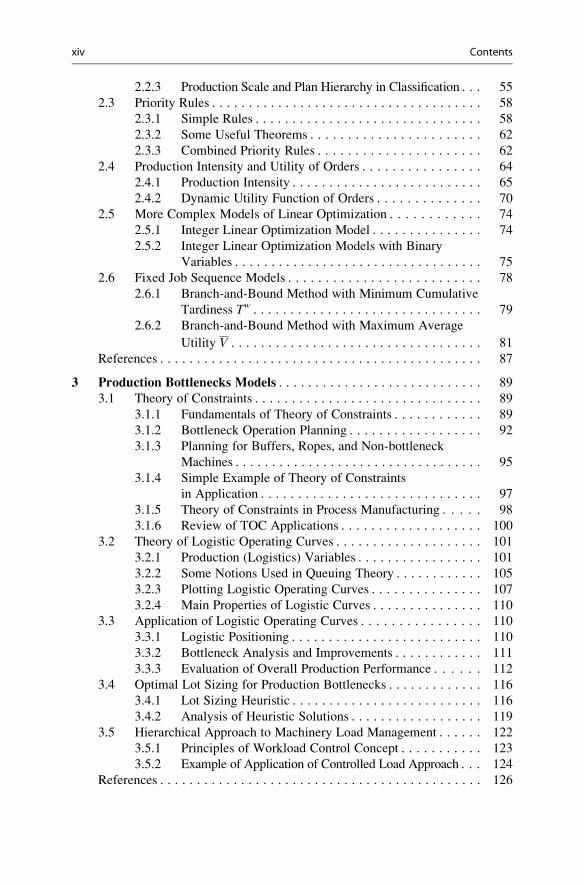
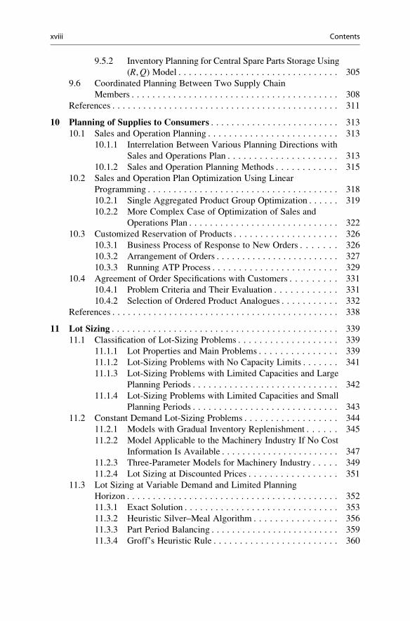
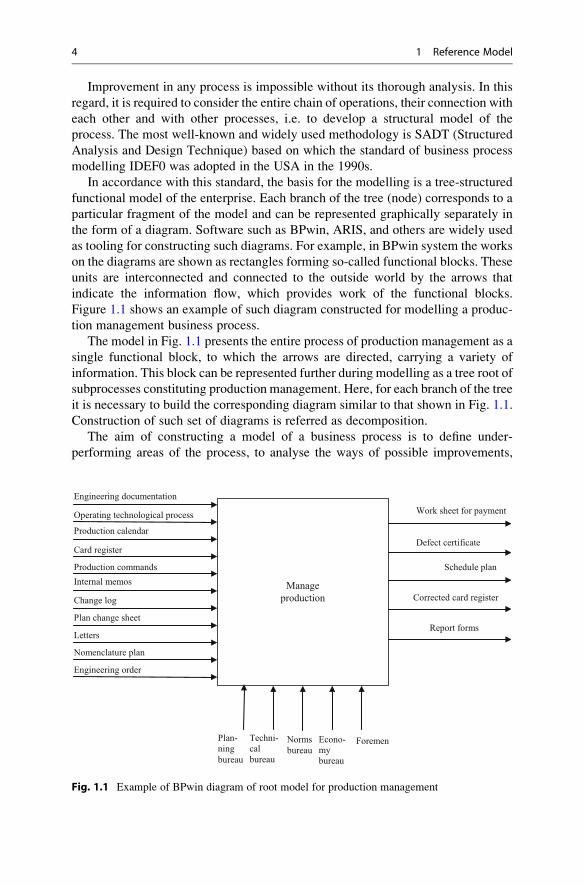
Figure 1.1 shows an example of such diagram constructed for modelling a produc-
tion management business process.
The model in Fig. 1.1 presents the entire process of production management as a
single functional block, to which the arrows are directed, carrying a variety of
information. This block can be represented further during modelling as a tree root of
subprocesses constituting production management. Here, for each branch of the tree
it is necessary to build the corresponding diagram similar to that shown in Fig. 1.1.
Construction of such set of diagrams is referred as decomposition.
The aim of constructing a model of a business process is to define under-
performing areas of the process, to analyse the ways of possible improvements,
Manage
production
Engineering documentation
Operating technological process
Production calendar
Card register
Production commands
Internal memos
Change log
Plan change sheet
Letters
Nomenclature plan
Engineering order
Work sheet for payment
Defect certificate
Schedule plan
Corrected card register
Report forms
Plan-ning
bureau
Techni-cal bureau
Norms
bureau
Econo-my bureau
Foremen
Fig. 1.1 Example of BPwin diagram of root model for production management
4 1 Reference Model
and to construct the model that is optimal in terms of model developers. The first
stage of this work is to construct AS-IS model, i.e. model of the existing business
processes. This model is built on the basis of study of available documentation and
interviews with employees of the enterprise.
Sequential analysis of AS-IS model taking into account operating experience of
existing business processes, its comparison with other similar examples, as well as
with the available scientific and technical recommendations allows developing a
new model that is currently optimal and real—TO-BE model. While constructing
this model one should not be misled about the real possibilities of the enterprise and
should not try to create a model that is ideal in terms of the customer or developer,
but has no chance of implementation—so-called SHOULD-BE model.
The constructed model allows us to make assessment of the business process
from different perspectives even before its start. The main requirements of the
enterprise activities are made for its operation, management, efficiency, outcomes
of activities, and customer satisfaction. Such analysis of business processes is called
an audit of business processes. During the audit, Activity Based Costing analysis is
made—measurement of costs and performance based on operations and costs of
objects. Simulation allows revealing components of the business process with the
highest cost and proposing improvements.
1.2 Concept of Reference Model
The analysis of the business process tree allows building the so-called reference
model. The main difference of the reference model is that a business process is
considered from several different viewpoints in it. Usually, there are two points of
view, but there may be others. From the first point of view, the reference model is a
certain standard of an efficient business process for an enterprise of a specific
industry; from the other point of view, it is a set of logically interrelated processes
containing references to the corresponding objects of the information system.
The two main properties are reflected by the word “reference”, which has two
meanings—“standard” and “link to”.
As a reference model, for example, the model of an existing business process,
which has the highest efficiency in the industry and uses quite complete information
system for its work, can be used. The reference models incorporating proven
procedures and methods of control enable enterprises to start developing their
own models on the basis of a ready set of business processes.
For this kind of development using the reference model, it is possible to divide
the entire business process into its component parts and distribute tasks to elaborate
an appropriate information system among the performers. In the course of work, the
available reference model allows all participants to discuss achieved results in the
framework of the terminology used in this model, which facilitates their interaction
greatly. The reference model analysis allows elaborating quality indices, which will
be discussed below. Finally, the availability of a detailed reference model allows
1.2 Concept of Reference Model 5
evaluating of the acceptability of a particular information system suggested for
implementation at the enterprise.
1.2.1 Reference Models in Supply Chains
The reference model concept started to be used first of all while analysing business
processes in the supply chains created at the stages of manufacturing and sales.
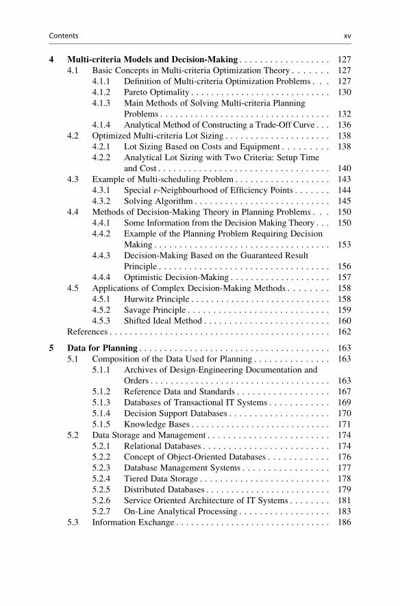
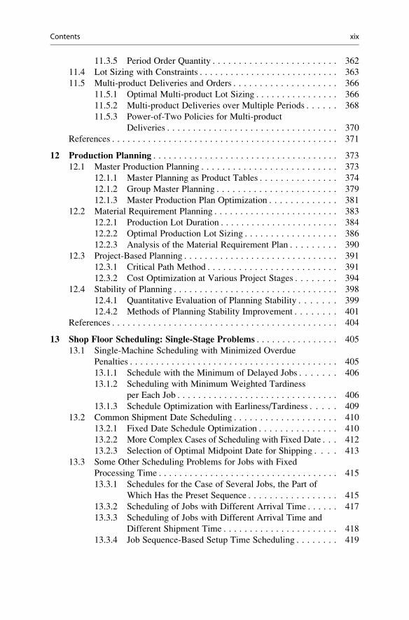
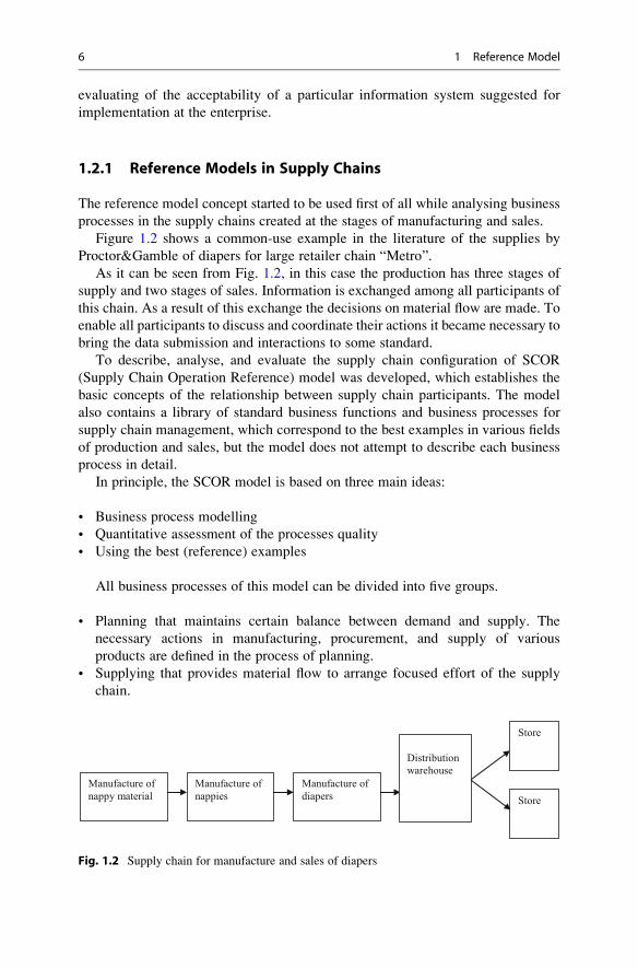
Figure 1.2 shows a common-use example in the literature of the supplies by
Proctor&Gamble of diapers for large retailer chain “Metro”.
As it can be seen from Fig. 1.2, in this case the production has three stages of
supply and two stages of sales. Information is exchanged among all participants of
this chain. As a result of this exchange the decisions on material flow are made. To
enable all participants to discuss and coordinate their actions it became necessary to
bring the data submission and interactions to some standard.
To describe, analyse, and evaluate the supply chain configuration of SCOR
(Supply Chain Operation Reference) model was developed, which establishes the
basic concepts of the relationship between supply chain participants. The model
also contains a library of standard business functions and business processes for
supply chain management, which correspond to the best examples in various fields
of production and sales, but the model does not attempt to describe each business
process in detail.
In principle, the SCOR model is based on three main ideas:
• Business process modelling
• Quantitative assessment of the processes quality
• Using the best (reference) examples
All business processes of this model can be divided into five groups.
• Planning that maintains certain balance between demand and supply. The
necessary actions in manufacturing, procurement, and supply of various
products are defined in the process of planning.
• Supplying that provides material flow to arrange focused effort of the supply
chain.
Manufacture of
nappy material
Manufacture of
nappies
Manufacture of
diapers
Distribution warehouse
Store
Store
Fig. 1.2 Supply chain for manufacture and sales of diapers
6 1 Reference Model
• Manufacturing, which generates new products.
• Delivery of finished products and services to the distribution and consumption
points.
• Return of the goods to the production or recycling sites. The return is possible for
different reasons, e.g. expired shelf life, wearing out, or obsolescence.
Each business process of the supply chain is defined by the so-called functional
attributes (Stadtler and Kilger 2008). For example, for the manufacture process the
attributes (indices) describing the organization of this process, extent of operations
repeatability, the presence of bottle necks, flexibility of working time use, setup
cost, etc. are very important. Accordingly, the process of distribution is described
by the scheme of products delivery, availability of vehicles and the limits of their
load capacity, etc. The functional attributes can be grouped by categories either
fully matching one of the processes or being part of the business process.
Stadtler and Kilger (2008) also specify that beside the functional attributes, the
values of the so-called structural attributes are essential for the supply chain. These
attributes are divided into two categories: topography and coordination. The first
category includes network structure, degree of globalization, and position of the
bottleneck in the network. The second category includes the following attributes:
balance of power of the chain elements, type of information exchanged, and legal
position of the entities in the supply chain.
1.2.2 Reference Modelling Methodology
Reference model according to the technique described in Hernandez et al. (2008) is
developed within six stages: information collection, evaluation, concept develop-
ment, modelling, check, and recommendations drawing up.
At the first stage, the application field (industry, enterprise, supply chain, etc.) of
the model is determined. The main entity objects of the described business process,
which specify obtaining, processing, and transferring of information, are defined.
At this point, the group of persons working on the model is determined and the main
goals of modelling are described.
At this stage, the model developers using the meetings with the enterprise
personnel and the documentation get familiar with the business-process objects to
be described when modelling. For instance, when modelling production manage-
ment, it is required to study issues of sales, supply, stock, production, and planning.
During such study, it might appear insufficient to work within the enterprise but
require studying the relations of the enterprise with other entities of the supply
chains.
Within the second stage, the processes that are described in the enterprise’s
collected documentation are studied. Besides, the study may involve the materials
from various systems connected with the modelling process. For example, when
modelling the process of production management, the issues of the quality
1.2 Concept of Reference Model 7
management, functionality of the applied information system, etc. may be studied
as well. The stage is intended to determine required technical and software tools for
the model development. When selecting these tools, one should consider not only
their functional features but also their cost, requirement for licensing, training level
of the developers, and possibilities to integrate with the existing information
system. In consequence of this stage, it is reasonable to develop a special document
describing the recommended tools for modelling.
At the stage of concept elaboration, the flows of products, information and
decisions in the modelled business process are considered. For the product flow,
the main production processes and existing constrains, e.g. capacities, are deter-
mined; the volumes of the existing demand and the extent of its satisfaction,
predictions of the demand in future, average-in-time stocks and their fluctuations
are defined. Production planning and management methods, as well as the produc-
tion stability are evaluated; economic performance of the production and its
profitability are studied. The results of the product flow study are suggested to be
stored in a document named PFDO (product flow document).
The study of the information flow considers the following aspects: list of the
main inputs of the business process and transformation of information in the
business process. The flow of decisions include the mechanism of the decision
making; objects, which are the matter of the decision; main actions of the personnel
on the decisions implementation and their interaction. For the information flow and
decision flow, it is recommended to draw up special documents named IFDO
(information flow document) and DFDO (decision flow document).
At the fourth stage, the modelling itself is performed, i.e. based on the
preselected tools and elaborated documents the model of the business process is
made. It is suggested to name the relevant document as CMDO (conceptual model
document). This document is checked at the fifth stage of development for compli-
ance with the main objectives, objects, and flows of the existing business process.
This stage finalizes construction of AS-IS-model.
The sixth stage of development is dedicated to the recommendation statement
on transformation of the existingmodel to newTO-BE-model. These recommendations
should describe the objects, which are necessary to be introduced orwhichmust replace
the existing objects of the business process and determine reasonable changes in
relations of the process entities.
The described technique can be actually used to business processes of any type.
Since in this book we consider mainly the issues of the production planning, the
reference models described here refer to this process. The planning reference model
pattern depends heavily on the production organization—“push” or “pull”.
It is known that the “push” organization moves the material flow from one
executor to each subsequent recipient strictly by the order (command) going from
the management centre of local (work, shop, site) or general (enterprise) produc-
tion. The “pull” production to the contrary provides determination of product
volumes at each production stage according to the needs of the following stages
solely.
8 1 Reference Model

1.3 Production Description
To build the reference model of planning the specific characteristics of production
must be taken into account. It is often assumed that planning should be performed in
different ways depending on whether the production is discrete or process. It is to be
recalled that in the discrete production the product units are the pieces, and in
process production—mass or volume. However, both of these types of production
have a significant common property, which is that in all cases the final product is
shipped to the consumer in the amount of one or more batches.
If we consider the process production, it is necessary to distinguish between two
of its kind: periodic and continuous. In the periodic process production, all its stages
are performed sequentially in a single apparatus, but in the continuous one—
simultaneously in different apparatuses. Instead of term “apparatus” typical for
process production hereinafter we shall always use more general term “machine”.
In the periodic production, of course, finished products are discharged from the
machine after a processing period in the form of a batch. In the continuous
production, despite the continuity of the process itself, the products can be extracted
by parts as well, which also form a batch. Since the main objective of planning is
to determine the batch size and the interval between them, the use of “batch-sized”
property of the products allows unified planning for discrete and process
production.
In terms of use of various methods of planning, the most important characteristics
of the production are its technical structure, scale, and production strategy.
1.3.1 Basic Types of Production
The production possibilities are defined by its technical structure which must meet
the number of requirements as follows:
• Compliance with the technological processes of finished product output;
• Compliance with the production scale;
• Possibility to simultaneously manufacture core and by-products;
• Provision of the external orders input into the system at its different points and
correct flow of the orders inside the system.
We can provide the indicative list of the basic types of production based on these
requirements and considering the possibility of concurrent use of machines with
different capacities in the system. This list (Mauergauz 2012) is based on the
analysis of a number of reported classifications compiled in terms of use of different
methods of planning for different types of production.
1.3 Production Description 9
Type 1. Single machine.
(a) It is fit to make only one type of product at a moment of time.
(b) It produces several types of products (core and by-products) simultaneously.
(c) It produces several orders as a single batch simultaneously.
Type 2. Parallel machines.
(a) Identical machines producing single type of product at a moment of time.
(b) Identical machines producing several kinds of products (core and by-products)
simultaneously.
(c) Different unrelated machines that produce single type of products at a moment
of time.
(d) Different unrelated machines that produce several kinds of products (core and
by-products) simultaneously.
Type 3. Synchronized flow shop manufacturing with given cycle.
(a) Automated production line.
(b) Versatile transfer line, producing single type of products at a moment of time.
(c) Versatile transfer line, producing several kinds of products (core and
by-products) simultaneously.
(d) Flexible assembly line.
(e) Complex multistage manufacturing that produces a set of core and by-products.
Type 4. Unsynchronized flow shop manufacturing (cell manufacturing).
Type 5. Job shop manufacturing.
(a) Set of individual machines.
(b) Set of technological sites (work centers).
(c) Set of individual workshops.
Type 6. Project manufacturing.
In every production type, there are raw materials and orders, which are input
parameters; core and by-products are output parameters. In the flow manufacturing
main production output comes out at the end of production line. By-products are
made at intermediate stages. Complex multistage manufacturing represents set of
serial and parallel lines with interdependent products. In single stage manufacturing
all kinds of production may be of equal importance.
Figure 1.3 shows two schemes of single stage manufacturing. Four versions of
flow shop manufacturing are shown in Figs. 1.4, 1.5 and 1.6 which demonstrate the
schemes of job shop and project manufacturing accordingly. The examples of the
complex multistage production will be presented below.
10 1 Reference Model
Solid arrows of three types shown in Fig. 1.3a designate raw material, core, and
by-products accordingly, and the dashed arrow designates external orders. Brace in
Fig. 1.3b means that external orders are to be fulfilled on any of the parallel
machines. Similar designations are used in Figs. 1.4–1.6. From the perspective of
b)
By-product
Core productOrders
a)
Raw material
Fig. 1.3 Two types of one-stage production: (a) type 1b; (b) type 2d
Orders
Core product
By-productsAdditional orders
Main
orders
Finished products
Main
orders
Staff
assemblerAdditional
assembler
c)
Additional orders
Working areas of conveyor
Coreproduct
Orders
Semi-finished
product
Finished
product
Raw materials
Buffers
Machinesa)
By-products
b)
d)
Fig. 1.4 Four types of flow-line production: (а) type 3a; (b) type 3b; (c) type 3c; (d) type 4
1.3 Production Description 11
planning, the machines can mean not only a physical piece of equipment but a
group of equipment (work centers), workshop, and even the whole enterprise. This
allows drawing up plans uniformly, which is often used to prepare plans of different
levels using MES-systems.
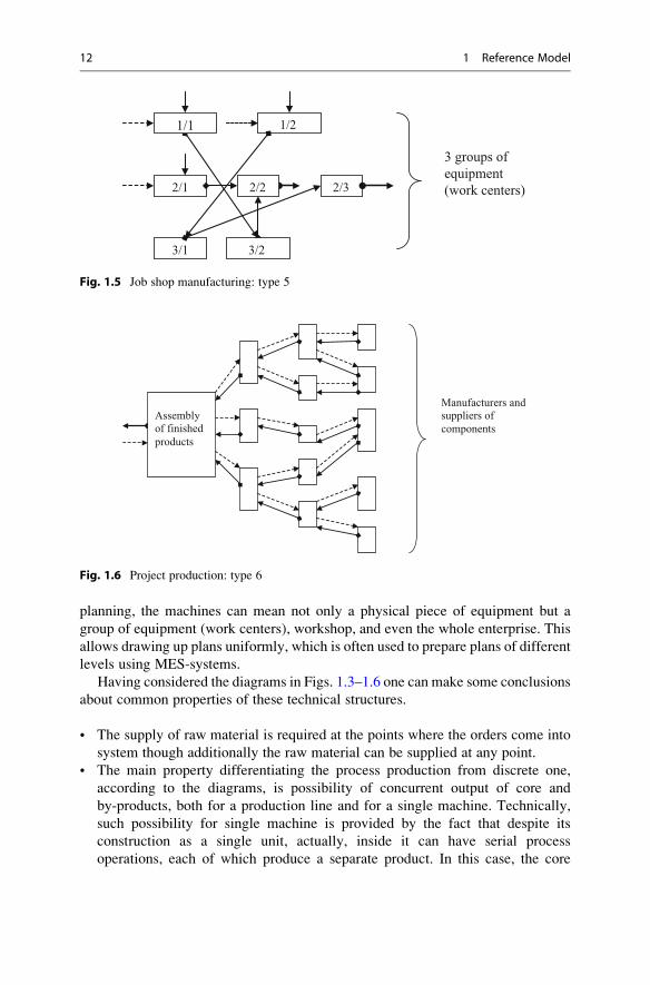
Having considered the diagrams in Figs. 1.3–1.6 one can make some conclusions
about common properties of these technical structures.
• The supply of raw material is required at the points where the orders come into
system though additionally the raw material can be supplied at any point.
• The main property differentiating the process production from discrete one,
according to the diagrams, is possibility of concurrent output of core and
by-products, both for a production line and for a single machine. Technically,
such possibility for single machine is provided by the fact that despite its
construction as a single unit, actually, inside it can have serial process
operations, each of which produce a separate product. In this case, the core
1/1 1/2
2/1 2/2 2/3
3/1 3/2
3 groups of
equipment
(work centers)
Fig. 1.5 Job shop manufacturing: type 5
Manufacturers and suppliers of
components
Assembly of finished
products
Fig. 1.6 Project production: type 6
12 1 Reference Model

product shall be considered to be the product after the last operation, and the rest
products are by-products.
• If orders are input directly at internal points of the production system, flow rate
may be supported by additional workers in a kind of buffer zone. In the systems,
where the synchronization of the machines in the flow is not available, entering
additional orders at separate points improves the quality of planning.
• The job shop manufacturing exists only for discrete production. Figure 1.5
shows possible order flow in production for three groups of uniform equipment.
• The project manufacturing features full matching of order tree and product tree,
the branch direction of which are opposite. Due to that feature, finished product
is produced in the same place where the initial order was entered.
It should be noted that in the versatile transfer lines of types 3b and 3c the
changes in the lines can occur not only during changeover of the whole line for
other type of product but also during setups of individual machines for different
process operations of the continuously produced product. The example of such line
is presented below in Sect. 7.3.
Table 1.1 shows correspondence of the main types of production 1–5 and
discrete and process production classification suggested by Pinedo (2005). As we
can see from this table, the above listed types of production indeed provide
description of both discrete and process production.
1.3.2 Production Scale and Strategy
Practical selection of a particular technical structure of production is closely
associated with its scale (Table 1.2).
Table 1.1 Correspondence of the basic types of production and classification by M. Pinedo
Types of production acc. to M.Pinedo Basic types of production
Process production
1a. Main processes of continuous
production
Single machine—type 1b; unrelated parallel
machines—type 2b, 2d; versatile transfer line—type
3c, 3e.
1b. Processes of preparation or final
processing in continuous production
Single machine—type 1a; unrelated parallel
machines—type 2a, 2c; versatile transfer line—type
3a, 3b; cell manufacturing—type 4.
Discrete production
2a. Procuring processes in discrete
production
Single machine—type 1a; unrelated parallel
machines—type 2a, 2c; cell manufacturing—type 4.
2b. Main processes of processing in
discrete production
Single machine—type 1a; unrelated parallel
machines—type 2a, 2c; versatile transfer line—type
3a, 3b; cell manufacturing—type 4; multipurpose
production—type 5a.
2c. Assembly processes in discrete
production
Flexible assembly line—type 3d; cell
manufacturing—type 4; project production—type 6
1.3 Production Description 13
The use of a single machine is the most versatile in terms of scale. More complex
technical structures tend either to large- or to small-scale production. Intermediate
example is the case of nonsynchronized flow production (cell manufacturing)
where the line method (typical for large-scale production) is combined with some
features of the job shop manufacturing.
The production strategy describes the products readiness to meet consumer
demand. This readiness determines the speed of response of the production enter-
prise to the received orders and influences the status of the enterprise on the market.
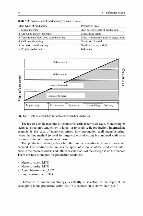
There are four strategies for production readiness:
• Make-to-stock, MTS
• Make-to-order, MTO
• Assemble-to-order, ATO
• Engineer-to-order, ETO
Difference in production strategy is actually in selection of the depth of the
decoupling in the production activities. This connection is shown in Fig. 1.7.
Table 1.2 Association of production type with its scale
Main types of production Production scale
1. Single machine Any possible scale of production
2. Unrelated parallel machines Mass, large serial
3. Synchronized flow shop manufacturing Mass with modifications or large serial
4. Cell manufacturing Serial, small serial
5. Job shop manufacturing Small serial, individual
6. Project production Individual
Engineering Procurement Processing Assembling Delivery
Man
ufa
ctu
rer
Cu
stomer
Make-to-stock
Make-to-order
Assemble-to-order
Engineer-to-order
Fig. 1.7 Depth of decoupling for different production strategies
14 1 Reference Model
In Fig. 1.7, we can see that the decoupling point, corresponding to the border of
the grey area, moves into the depth of the production activity so far as the strategy
approaches to the tracing of the external orders.
Selection of the production strategy is influenced by the duration of the
production cycle, the admissible waiting time for order fulfilment in competitive
environment, need for adjustment of the product to the customer’s requirements,
availability of enough current assets, etc.
1.4 Advanced Planning in IT Systems
The purpose of the application of any reference model is to improve the enterprise
management. As the efficient management in the present market economy is
impossible without use of modern methods of planning, an adequate reference
model of the planning process needs to be built because it is a necessary step in
the management upgrading. Reference model of planning is the foundation
on which it is possible to use different mathematical models, recommendations
for decision-making and other methods that are currently unified by concept
“advanced” planning.
The main difference of methods Advanced Planning and Scheduling, AP&S, is
not so much the use of mathematical methods for finding optimal solutions as the
idea of planning as a dynamic process. This method of planning usually uses a
concept of “sliding” horizon, which means that at every moment of planning the
plan decision is prepared for a certain upcoming interval of time, which does not
necessarily have to be permanent.
The second feature of the Advanced Planning and Scheduling is a compulsory
evaluation of available information to support the decisions to be made. Thus, as a
rule, quality criteria of decisions are set and the methods of achieving high values of
these criteria are selected.
The third essential feature of this approach is consideration of various
constraints, especially regarding capacity, immediately in the planning process.
1.4.1 Planning in IT Systems
Since the nature of the planning decision generally depends on the interval duration,
i.e. on the planning horizon, in the information systems that support production
planning, there are several levels of planning. Currently, there are four types of
information systems which provide the planning of production and supply at
different levels:
• Enterprise Resource Planning, ERP
• Manufacturing Execution System, MES
• Advanced Planning System, APS
• Supply Chain Management, SCM
1.4 Advanced Planning in IT Systems 15
One should distinguish AP&S approach from APS-systems as such. Certainly,
that the specially developed APS-systems use AP&S approach, however, the latter
can be used in various other systems including ERP-systems. Table 1.3 presents
planning possibilities at different levels for the above listed systems.
Table 1.3 shows five possible levels of planning. As seen from the table, none of
the above types of information systems involve the use of each of these levels. The
most common (and early developed) ERP-systems usually do not have the level of
strategic (business) planning, but have a complete set of functions for production
planning including scheduling at the workshop level. ERP-systems belong to the
class of so-called transaction systems, where each business transaction is associated
with initial data accumulation or its processing to get reports on the data.
In newMES-systems and certainly in special APS-systems, optimization models
are used, which function on the basis of a dedicated database. This database is
created in the framework of the reference model and required for decision-making.
When the first APS-systems were under development, it was supposed that their
application field will be very wide—from the corporate to the workshop level.
Moreover, all these levels were to be provided by three types of planning—long-
term (strategic), medium-term (tactical), and short-term (operational) (Stadtler and
Kilger 2008; Shapiro 2001). Since APS-systems do not have initial data on
products, equipment, personnel, etc., their operation is only possible in combination
with ERP-systems. Besides, to perform the tasks it is necessary to reload the data
into the APS-system, add the data required for decisions and missing in
ERP-system into this system, and return the obtain results to the ERP-system for
their application.
Application of such complex data processing mechanism has led to rather
limited capabilities of APS-systems in practice. Currently, these systems seem
reasonable to be used at the level of a strategic plan for the corporation in general
and the individual enterprise as well as at the level of preparation of master
production schedule. Short-term planning using these systems typically is reason-
able for a large-scale process production with a relatively large (for a week or more)
planning horizon. Table 1.4 lists the main modules that make up the structure of
some APS-systems.
APS-systems, listed in Table 1.4 are intended for a large range of scheduled
tasks in various industries, and, respectively, are provided with a number of
powerful planning modules. These systems, for the most part, are developed by
the same company that developed ERP-systems and are in fact superstructures over
the latter. Such APS-systems are quite expensive and their use is rather difficult.
There are also specialized simpler and cheaper APS-systems that perform
particular planning tasks. However, to use these systems effectively, adequate
matching of their capabilities and features of a specific task is required. A success-
ful example can be the use of Lawson M3 Supply Chain Planner for the task of
optimal planning of seed stocks and their distribution among farmers (Andersson
and Rudberg 2007). These systems usually have units that provide the possibility of
their cooperation with various ERP-systems, which allows selecting the best
16 1 Reference Model
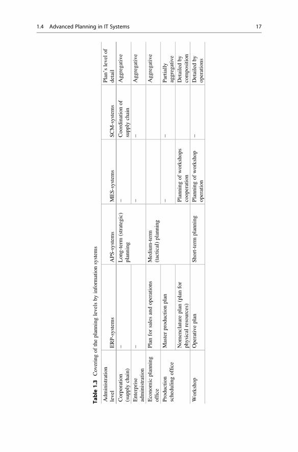
Table
1.3
Coveringoftheplanninglevelsbyinform
ationsystem
s
Administration
level
ERP-system
sAPS-system
sMES-system
sSCM-system
s
Plan’slevel
of
detail
Corporation
(supply
chain)
–Long-term
(strategic)
planning
–Coordinationof
supply
chain
Aggregative
Enterprise
administration
––
–Aggregative
Economic
planning
office
Planforsalesandoperations
Medium-term
(tactical)planning
Aggregative
Production
schedulingoffice
Masterproductionplan
––
Partially
aggregative
Nomenclature
plan(planfor
physicalresources)
Planningofworkshops
cooperation
Detailedby
composition
Workshop
Operativeplan
Short-term
planning
Planningofworkshop
operation
–Detailedby
operations
1.4 Advanced Planning in IT Systems 17
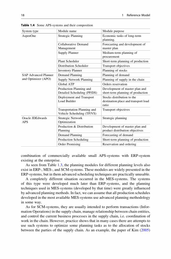
combination of commercially available small APS-systems with ERP-system
existing at the enterprise.
As seen from Table 1.3, the planning modules for different planning levels also
exist in ERP-, MES-, and SCM-systems. These modules are widely presented in the
ERP-systems, but in them advanced scheduling techniques are practically unusable.
A completely different situation occurred in the MES-systems. The systems
of this type were developed much later than ERP-systems, and the planning
techniques used in MES-systems (developed by that time) were greatly influenced
by advanced planning methods. In fact, we can assume that all production schedules
developed in the most available MES-systems use advanced planning methodology
in some way.
As for SCM-systems, they are usually intended to perform transactions (Infor-
mation Operations) in the supply chain, manage relationship between chain entities,
and control the current business processes in the supply chain, i.e. coordination of
work in the chain. However, practice shows that in many cases there are attempts to
use such systems to optimize some planning tasks as to the allocation of stocks
between the parties of the supply chain. As an example, the paper of Kim (2005)
Table 1.4 Some APS-systems and their composition
System type Module name Module purpose
AspenOne Strategic Planning Economic tasks of long-term
planning.
Collaborative Demand
Management
Forecasting and development of
master plan
Supply Planner Medium-term planning of
procurement
Plant Scheduler Short-term planning of production
Distribution Scheduler Transport objectives
Inventory Planner Planning of stocks
SAP Advanced Planner
and Optimizer (APO)
Demand Planning Planning of demand
Supply Network Planning Planning of supply in the chain
Global ATP Orders reservation
Production Planning and
Detailed Scheduling (PP/DS)
Development of master plan and
short-term planning of production
Deployment and Transport
Load Builder
Stocks distribution to the
destination place and transport load
ratio
Transportation Planning and
Vehicle Scheduling (TP/VS)
Transport objectives
Oracle JDEdwards
APS
Strategic Network
Optimization
Strategic planning
Production & Distribution
Planning
Development of master plan and
product distribution objectives
Demand Planning Forecasting of demand
Production Scheduling Short-term planning of production
Order Promising Reservation and ordering
18 1 Reference Model
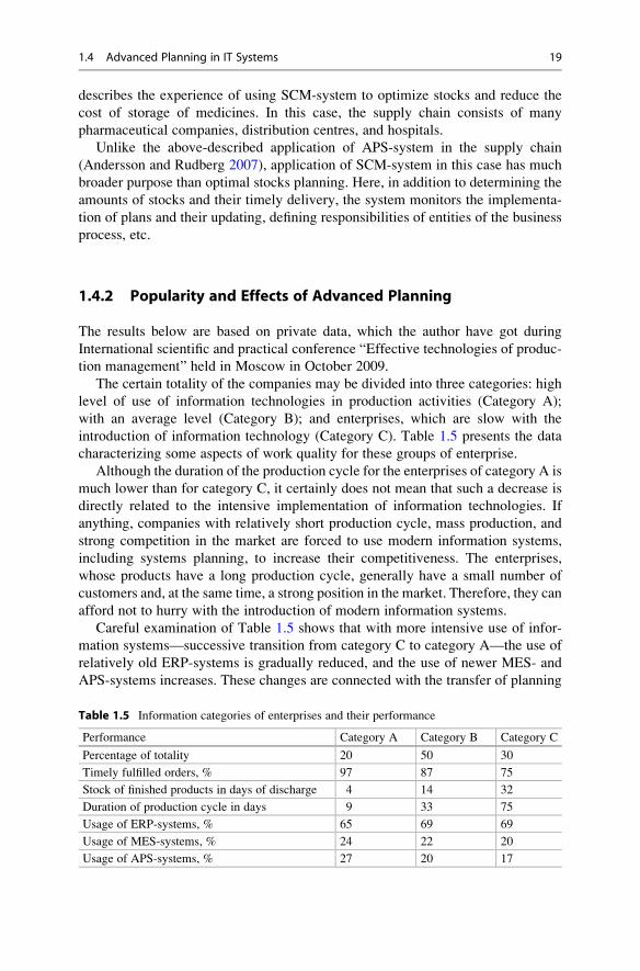
describes the experience of using SCM-system to optimize stocks and reduce the
cost of storage of medicines. In this case, the supply chain consists of many
pharmaceutical companies, distribution centres, and hospitals.
Unlike the above-described application of APS-system in the supply chain
(Andersson and Rudberg 2007), application of SCM-system in this case has much
broader purpose than optimal stocks planning. Here, in addition to determining the
amounts of stocks and their timely delivery, the system monitors the implementa-
tion of plans and their updating, defining responsibilities of entities of the business
process, etc.
1.4.2 Popularity and Effects of Advanced Planning
The results below are based on private data, which the author have got during
International scientific and practical conference “Effective technologies of produc-
tion management” held in Moscow in October 2009.
The certain totality of the companies may be divided into three categories: high
level of use of information technologies in production activities (Category A);
with an average level (Category B); and enterprises, which are slow with the
introduction of information technology (Category C). Table 1.5 presents the data
characterizing some aspects of work quality for these groups of enterprise.
Although the duration of the production cycle for the enterprises of category A is
much lower than for category C, it certainly does not mean that such a decrease is
directly related to the intensive implementation of information technologies. If
anything, companies with relatively short production cycle, mass production, and
strong competition in the market are forced to use modern information systems,
including systems planning, to increase their competitiveness. The enterprises,
whose products have a long production cycle, generally have a small number of
customers and, at the same time, a strong position in the market. Therefore, they can
afford not to hurry with the introduction of modern information systems.
Careful examination of Table 1.5 shows that with more intensive use of infor-
mation systems—successive transition from category C to category A—the use of
relatively old ERP-systems is gradually reduced, and the use of newer MES- and
APS-systems increases. These changes are connected with the transfer of planning
Table 1.5 Information categories of enterprises and their performance
Performance Category A Category B Category C
Percentage of totality 20 50 30
Timely fulfilled orders, % 97 87 75
Stock of finished products in days of discharge 4 14 32
Duration of production cycle in days 9 33 75
Usage of ERP-systems, % 65 69 69
Usage of MES-systems, % 24 22 20
Usage of APS-systems, % 27 20 17
1.4 Advanced Planning in IT Systems 19
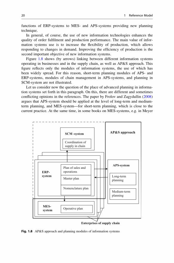
functions of ERP-systems to MES- and APS-systems providing new planning
technique.
In general, of course, the use of new information technologies enhances the
quality of order fulfilment and production performance. The main value of infor-
mation systems use is to increase the flexibility of production, which allows
responding to changes in demand. Improving the efficiency of production is the
second important objective of new information systems.
Figure 1.8 shows (by arrows) linking between different information systems
operating in businesses and in the supply chain, as well as AP&S approach. This
figure reflects only the modules of information systems, the use of which has
been widely spread. For this reason, short-term planning modules of APS- and
ERP-systems, modules of chain management in APS-systems, and planning in
SCM-system are not illustrated.
Let us consider now the question of the place of advanced planning in informa-
tion systems set forth in this paragraph. On this, there are different and sometimes
conflicting opinions in the references. The paper by Frolov and Zagydullin (2008)
argues that APS-system should be applied at the level of long-term and medium-
term planning, and MES-system—for short-term planning, which is close to the
current practice. At the same time, in some books on MES-systems, e.g. in Meyer
SCM -system
Coordination of supply in chain
Master plan
Nomenclature plan
ERP-system
MES-system Operative plan
APS-system
Long-term planning
Medium-term
planning
AP&S approach
Enterprises of supply chain
Plan of sales and
operations
Fig. 1.8 AP&S approach and planning modules of information systems
20 1 Reference Model
et al. (2009), it is suggested that APS-system should be included directly into the
MES-system.
Most probably, the last statement comes due to the fact that the book (Meyer
et al. 2009) identified the notion of APS-system and the AP&S approach. Indeed,
developers of MES-systems planning modules usually have to use the above basic
principles of AP&S approach from the very beginning, namely—responsiveness,
optimization, and constrains consideration as otherwise the estimated plans will be
either unrealistic or have low quality. At the same time inside the MES-system,
typically no particular APS-system exists.
Figure 1.8 shows ERP- and MES-systems as integral parts of the production
enterprise, and SCM-system as an object that is used to manage the chain of
enterprises and, accordingly, located over these enterprises. At the same time, the
presence of APS-system as a separate system is not necessary or even desirable
for the enterprise operation, and that is why APS-system is shown outside the
enterprise.
Currently, ideas and techniques of AP&S approach are implemented for
planning using APS- and MES-systems circled in Fig. 1.8 by the bold line.
However, it is quite possible that during development of new ERP- and
SCM-systems advanced planning methods will be included in them, and the need
for special APS-systems will gradually decrease. The dashed line in Fig. 1.8 shows
occurring in this case additional field of application of AP&S approach.
1.5 IT System Interaction Standards
Large variety of information systems in the market has required a certain ordering,
allowing users, firstly, to know their way around in this set of systems, and,
secondly, to assess the possibility of their cooperation. Simultaneously, within the
last two decades, the developers of information systems became aware of practica-
bility to standardize some aspects related to the objectives and interaction of the
systems.
Establishment of many public associations of developers and users of informa-
tion systems has been essential for elaboration of standardization issues. The
most famous associations are APICS (American Production and Inventory
Control Society), SCC (Supply Chain Council), MESA (Manufacturing Enterprise
Solutions Association), ISA (Instrumentation, Systems and Automation Society),
OPC Foundation, and others. As a rule, these associations elaborate not the standard
but some recommendations, which in case their wide-spreading are somehow
legalized by International Organizations for Standardization.
Standardization in information systems is performed mainly in three directions:
system structure and report documents; data; and information exchange methods.
In this Chapter, only the first direction is analysed and the others will be analysed
in Chap. 5.
The most famous example of the system structure standardization is
standard MRP2. Historically, first, association APICS developed a number of
1.5 IT System Interaction Standards 21
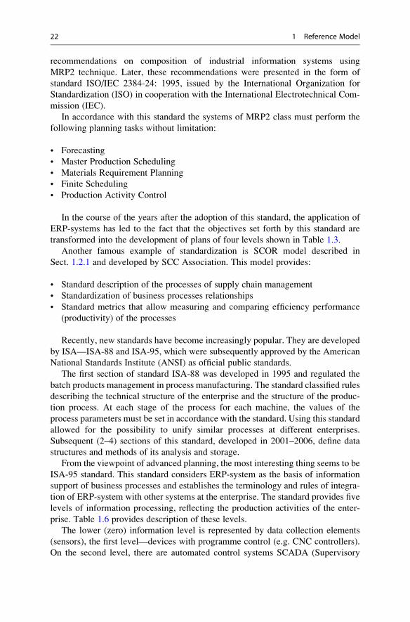
recommendations on composition of industrial information systems using
MRP2 technique. Later, these recommendations were presented in the form of
standard ISO/IEC 2384-24: 1995, issued by the International Organization for
Standardization (ISO) in cooperation with the International Electrotechnical Com-
mission (IEC).
In accordance with this standard the systems of MRP2 class must perform the
following planning tasks without limitation:
• Forecasting
• Master Production Scheduling
• Materials Requirement Planning
• Finite Scheduling
• Production Activity Control
In the course of the years after the adoption of this standard, the application of
ERP-systems has led to the fact that the objectives set forth by this standard are
transformed into the development of plans of four levels shown in Table 1.3.
Another famous example of standardization is SCOR model described in
Sect. 1.2.1 and developed by SCC Association. This model provides:
• Standard description of the processes of supply chain management
• Standardization of business processes relationships
• Standard metrics that allow measuring and comparing efficiency performance
(productivity) of the processes
Recently, new standards have become increasingly popular. They are developed
by ISA—ISA-88 and ISA-95, which were subsequently approved by the American
National Standards Institute (ANSI) as official public standards.
The first section of standard ISA-88 was developed in 1995 and regulated the
batch products management in process manufacturing. The standard classified rules
describing the technical structure of the enterprise and the structure of the produc-
tion process. At each stage of the process for each machine, the values of the
process parameters must be set in accordance with the standard. Using this standard
allowed for the possibility to unify similar processes at different enterprises.
Subsequent (2–4) sections of this standard, developed in 2001–2006, define data
structures and methods of its analysis and storage.
From the viewpoint of advanced planning, the most interesting thing seems to be
ISA-95 standard. This standard considers ERP-system as the basis of information
support of business processes and establishes the terminology and rules of integra-
tion of ERP-system with other systems at the enterprise. The standard provides five
levels of information processing, reflecting the production activities of the enter-
prise. Table 1.6 provides description of these levels.
The lower (zero) information level is represented by data collection elements
(sensors), the first level—devices with programme control (e.g. CNC controllers).
On the second level, there are automated control systems SCADA (Supervisory
22 1 Reference Model
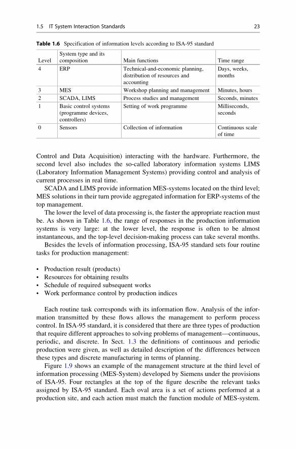
Control and Data Acquisition) interacting with the hardware. Furthermore, the
second level also includes the so-called laboratory information systems LIMS
(Laboratory Information Management Systems) providing control and analysis of
current processes in real time.
SCADA and LIMS provide information MES-systems located on the third level;
MES solutions in their turn provide aggregated information for ERP-systems of the
top management.
The lower the level of data processing is, the faster the appropriate reaction must
be. As shown in Table 1.6, the range of responses in the production information
systems is very large: at the lower level, the response is often to be almost
instantaneous, and the top-level decision-making process can take several months.
Besides the levels of information processing, ISA-95 standard sets four routine
tasks for production management:
• Production result (products)
• Resources for obtaining results
• Schedule of required subsequent works
• Work performance control by production indices
Each routine task corresponds with its information flow. Analysis of the infor-
mation transmitted by these flows allows the management to perform process
control. In ISA-95 standard, it is considered that there are three types of production
that require different approaches to solving problems of management—continuous,
periodic, and discrete. In Sect. 1.3 the definitions of continuous and periodic
production were given, as well as detailed description of the differences between
these types and discrete manufacturing in terms of planning.
Figure 1.9 shows an example of the management structure at the third level of
information processing (MES-System) developed by Siemens under the provisions
of ISA-95. Four rectangles at the top of the figure describe the relevant tasks
assigned by ISA-95 standard. Each oval area is a set of actions performed at a
production site, and each action must match the function module of MES-system.
Table 1.6 Specification of information levels according to ISA-95 standard
Level
System type and its
composition Main functions Time range
4 ERP Technical-and-economic planning,
distribution of resources and
accounting
Days, weeks,
months
3 MES Workshop planning and management Minutes, hours
2 SCADA, LIMS Process studies and management Seconds, minutes
1 Basic control systems
(programme devices,
controllers)
Setting of work programme Milliseconds,
seconds
0 Sensors Collection of information Continuous scale
of time
1.5 IT System Interaction Standards 23
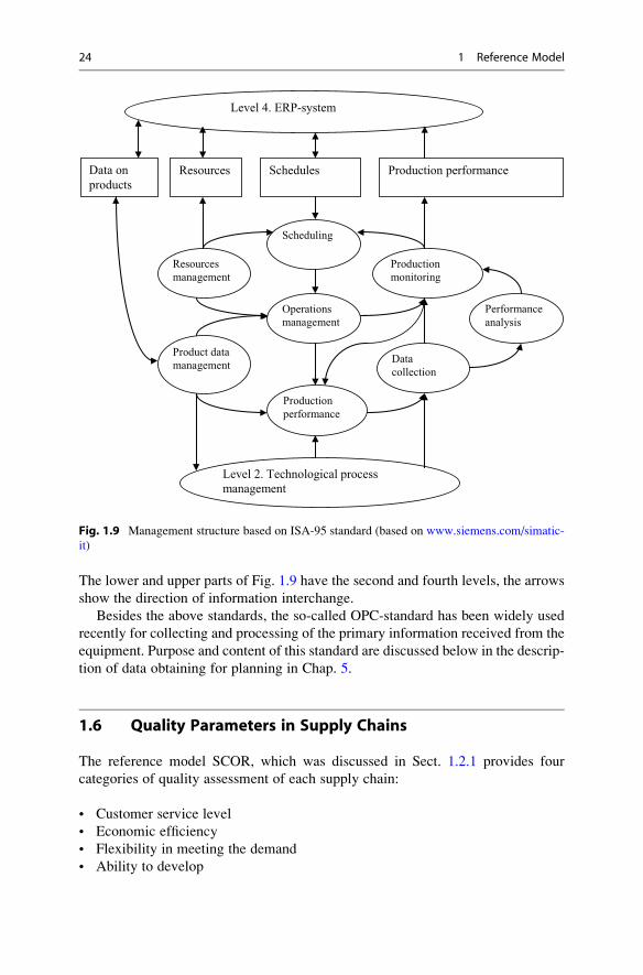
The lower and upper parts of Fig. 1.9 have the second and fourth levels, the arrows
show the direction of information interchange.
Besides the above standards, the so-called OPC-standard has been widely used
recently for collecting and processing of the primary information received from the
equipment. Purpose and content of this standard are discussed below in the descrip-
tion of data obtaining for planning in Chap. 5.
1.6 Quality Parameters in Supply Chains
The reference model SCOR, which was discussed in Sect. 1.2.1 provides four
categories of quality assessment of each supply chain:
• Customer service level
• Economic efficiency
• Flexibility in meeting the demand
• Ability to develop
Data on
productsResources Schedules Production performance
Resources
management
Product data
management
Scheduling
Operations
management
Production
performance
Production
monitoring
Data
collection
Performance
analysis
Level 2. Technological process management
Level 4. ERP-system
Fig. 1.9 Management structure based on ISA-95 standard (based on www.siemens.com/simatic-
it)
24 1 Reference Model
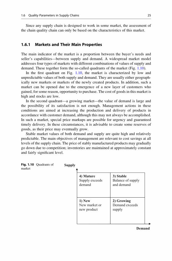
Since any supply chain is designed to work in some market, the assessment of
the chain quality chain can only be based on the characteristics of this market.
1.6.1 Markets and Their Main Properties
The main indicator of the market is a proportion between the buyer’s needs and
seller’s capabilities—between supply and demand. A widespread market model
addresses four types of markets with different combinations of values of supply and
demand. These together form the so-called quadrants of the market (Fig. 1.10).
In the first quadrant on Fig. 1.10, the market is characterized by low and
unpredictable values of both supply and demand. They are usually either geograph-
ically new markets or markets of the newly created products. In addition, such a
market can be opened due to the emergence of a new layer of customers who
gained, for some reason, opportunity to purchase. The cost of goods in this market is
high and stocks are low.
In the second quadrant—a growing market—the value of demand is large and
the possibility of its satisfaction is not enough. Management actions in these
conditions are aimed at increasing the production and delivery of products in
accordance with customer demand, although this may not always be accomplished.
In such a market, special price markups are possible for urgency and guaranteed
timely delivery. In these circumstances, it is advisable to create some reserves of
goods, as their price may eventually grow.
Stable market values of both demand and supply are quite high and relatively
predictable. The main objectives of management are relevant to cost savings at all
levels of the supply chain. The price of stably manufactured products may gradually
go down due to competition; inventories are maintained at approximately constant
and fairly significant level.
Supply
Demand
1) NewNew market or
new product
2) GrowingDemand exceeds
supply
4) MatureSupply exceeds
demand
3) StableBalance of supply
and demand
Fig. 1.10 Quadrants of
market
1.6 Quality Parameters in Supply Chains 25
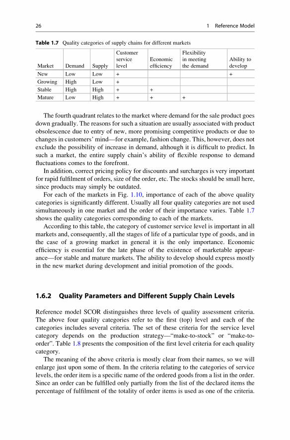
The fourth quadrant relates to the market where demand for the sale product goes
down gradually. The reasons for such a situation are usually associated with product
obsolescence due to entry of new, more promising competitive products or due to
changes in customers’ mind—for example, fashion change. This, however, does not
exclude the possibility of increase in demand, although it is difficult to predict. In
such a market, the entire supply chain’s ability of flexible response to demand
fluctuations comes to the forefront.
In addition, correct pricing policy for discounts and surcharges is very important
for rapid fulfilment of orders, size of the order, etc. The stocks should be small here,
since products may simply be outdated.
For each of the markets in Fig. 1.10, importance of each of the above quality
categories is significantly different. Usually all four quality categories are not used
simultaneously in one market and the order of their importance varies. Table 1.7
shows the quality categories corresponding to each of the markets.
According to this table, the category of customer service level is important in all
markets and, consequently, all the stages of life of a particular type of goods, and in
the case of a growing market in general it is the only importance. Economic
efficiency is essential for the late phase of the existence of marketable appear-
ance—for stable and mature markets. The ability to develop should express mostly
in the new market during development and initial promotion of the goods.
1.6.2 Quality Parameters and Different Supply Chain Levels
Reference model SCOR distinguishes three levels of quality assessment criteria.
The above four quality categories refer to the first (top) level and each of the
categories includes several criteria. The set of these criteria for the service level
category depends on the production strategy—“make-to-stock” or “make-to-
order”. Table 1.8 presents the composition of the first level criteria for each quality
category.
The meaning of the above criteria is mostly clear from their names, so we will
enlarge just upon some of them. In the criteria relating to the categories of service
levels, the order item is a specific name of the ordered goods from a list in the order.
Since an order can be fulfilled only partially from the list of the declared items the
percentage of fulfilment of the totality of order items is used as one of the criteria.
Table 1.7 Quality categories of supply chains for different markets
Market Demand Supply
Customer
service
level
Economic
efficiency
Flexibility
in meeting
the demand
Ability to
develop
New Low Low + +
Growing High Low +
Stable High High + +
Mature Low High + + +
26 1 Reference Model
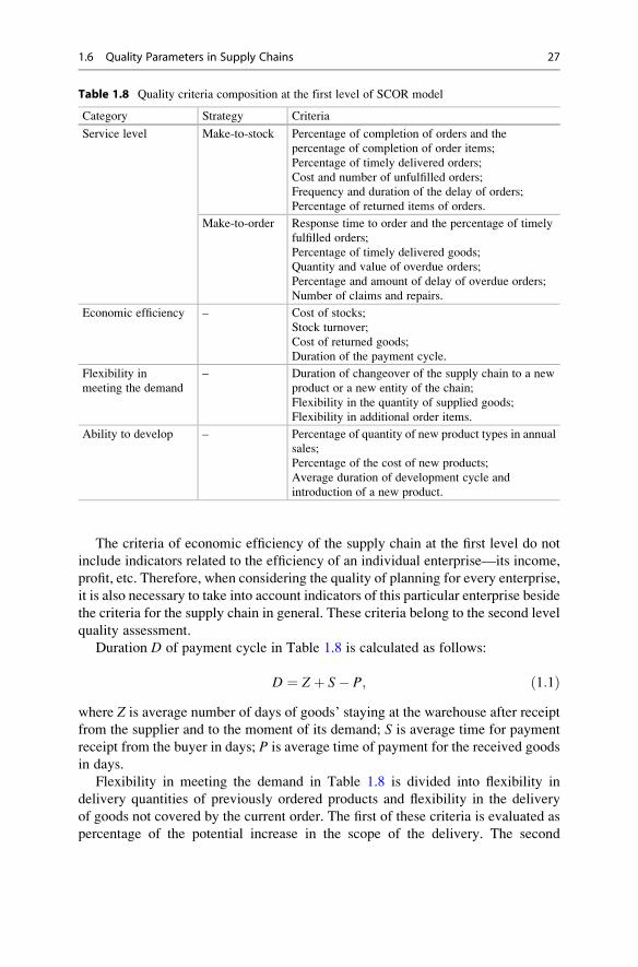
The criteria of economic efficiency of the supply chain at the first level do not
include indicators related to the efficiency of an individual enterprise—its income,
profit, etc. Therefore, when considering the quality of planning for every enterprise,
it is also necessary to take into account indicators of this particular enterprise beside
the criteria for the supply chain in general. These criteria belong to the second level
quality assessment.
Duration D of payment cycle in Table 1.8 is calculated as follows:
D ¼ Z þ S� P; ð1:1Þwhere Z is average number of days of goods’ staying at the warehouse after receipt
from the supplier and to the moment of its demand; S is average time for payment
receipt from the buyer in days; P is average time of payment for the received goods
in days.
Flexibility in meeting the demand in Table 1.8 is divided into flexibility in
delivery quantities of previously ordered products and flexibility in the delivery
of goods not covered by the current order. The first of these criteria is evaluated as
percentage of the potential increase in the scope of the delivery. The second
Table 1.8 Quality criteria composition at the first level of SCOR model
Category Strategy Criteria
Service level Make-to-stock Percentage of completion of orders and the
percentage of completion of order items;
Percentage of timely delivered orders;
Cost and number of unfulfilled orders;
Frequency and duration of the delay of orders;
Percentage of returned items of orders.
Make-to-order Response time to order and the percentage of timely
fulfilled orders;
Percentage of timely delivered goods;
Quantity and value of overdue orders;
Percentage and amount of delay of overdue orders;
Number of claims and repairs.
Economic efficiency – Cost of stocks;
Stock turnover;
Cost of returned goods;
Duration of the payment cycle.
Flexibility in
meeting the demand
– Duration of changeover of the supply chain to a new
product or a new entity of the chain;
Flexibility in the quantity of supplied goods;
Flexibility in additional order items.
Ability to develop – Percentage of quantity of new product types in annual
sales;
Percentage of the cost of new products;
Average duration of development cycle and
introduction of a new product.
1.6 Quality Parameters in Supply Chains 27
criterion can be determined by the average percentage of substitution of previously
ordered goods by other goods.
The degree of application of the criteria from the list to evaluate the performance
of the supply chain is different depending on which of the five groups described in
Sect. 1.2.1 the considered business process belong to. For example, for business
processes from planning and procurement groups (Hugo 2006) criteria for the first
three categories in Table 1.8 are commonly used (in various combinations), and for
the processes of the group of manufacturing—practically all of the above criteria.
Standard SCOR states that except the first strategic level, the processes in the
supply chain should be evaluated on the second and third (tactical and operational)
levels as well. As mentioned above, the second level of evaluation includes (above
all) economic indicators defined in the business process of planning. The produc-
tion process is defined by the criteria of production cycle duration, level of product
quality, and timely execution of orders. In general, a set of criteria for the second
level should be sufficient for a complete and impartial assessment of the quality of
the current business processes.
The objective of the third level of evaluation is the so-called diagnostics of
business processes. The measured or calculated indices of this level should allow
managers identifying lower-level deficiencies of the ongoing process, deciding on
correction of production situation, and transmitting the required information to their
superiors. All figures in the third level are divided into three groups:
• Process complexity indices
• Characteristics of supply chains configurations
• Current parameters of the process
For example, for business process from the planning group the complexity
indicators are percentage of order changes, the number of goods items, volume of
production, and the cost of inventories. The configuration of the supply network for
the same group, i.e. for planning processes, is characterized by delivery scope in
one supply chain, the number of chains, and the placement of the supply chain.
To assess the current status of planning processes, it is recommended to use
parameters such as the duration of the planning cycle, forecasting accuracy, and the
percentage of available and obsolete inventories.
More detailed composition of criteria of the second and third levels of SCOR
standard is described in the book of Hugo (2006) and on the website www.supply-
chain.org. In SCOR standard, starting with version 8.0, the terminology is unified
with the terminology described above in Sect. 1.5 of ISA-95 standard.
1.6.3 Balanced Scorecard
Balanced Scorecard (BSC) is a concept for achieving company’s strategic goals by
purposeful actions at various levels of management. Figure 1.11 shows the rations
of main causes and effects defining the result of company’s performance.
28 1 Reference Model
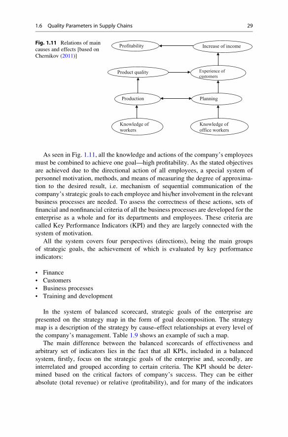
As seen in Fig. 1.11, all the knowledge and actions of the company’s employees
must be combined to achieve one goal—high profitability. As the stated objectives
are achieved due to the directional action of all employees, a special system of
personnel motivation, methods, and means of measuring the degree of approxima-
tion to the desired result, i.e. mechanism of sequential communication of the
company’s strategic goals to each employee and his/her involvement in the relevant
business processes are needed. To assess the correctness of these actions, sets of
financial and nonfinancial criteria of all the business processes are developed for the
enterprise as a whole and for its departments and employees. These criteria are
called Key Performance Indicators (KPI) and they are largely connected with the
system of motivation.
All the system covers four perspectives (directions), being the main groups
of strategic goals, the achievement of which is evaluated by key performance
indicators:
• Finance
• Customers
• Business processes
• Training and development
In the system of balanced scorecard, strategic goals of the enterprise are
presented on the strategy map in the form of goal decomposition. The strategy
map is a description of the strategy by cause–effect relationships at every level of
the company’s management. Table 1.9 shows an example of such a map.
The main difference between the balanced scorecards of effectiveness and
arbitrary set of indicators lies in the fact that all KPIs, included in a balanced
system, firstly, focus on the strategic goals of the enterprise and, secondly, are
interrelated and grouped according to certain criteria. The KPI should be deter-
mined based on the critical factors of company’s success. They can be either
absolute (total revenue) or relative (profitability), and for many of the indicators
Profitability Increase of income
Experience of customers
Product quality
PlanningProduction
Knowledge of workers
Knowledge of office workers
Fig. 1.11 Relations of main
causes and effects [based on
Chernikov (2011)]
1.6 Quality Parameters in Supply Chains 29
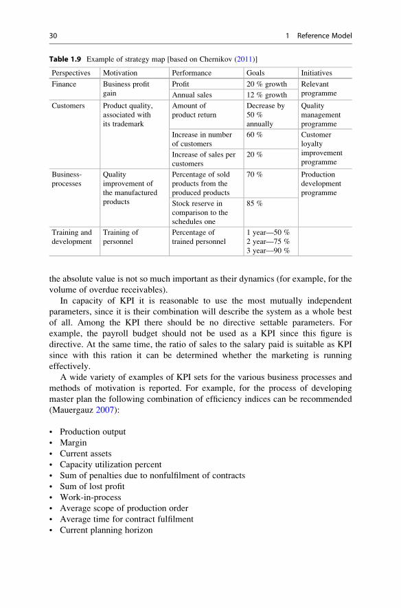
the absolute value is not so much important as their dynamics (for example, for the
volume of overdue receivables).
In capacity of KPI it is reasonable to use the most mutually independent
parameters, since it is their combination will describe the system as a whole best
of all. Among the KPI there should be no directive settable parameters. For
example, the payroll budget should not be used as a KPI since this figure is
directive. At the same time, the ratio of sales to the salary paid is suitable as KPI
since with this ration it can be determined whether the marketing is running
effectively.
A wide variety of examples of KPI sets for the various business processes and
methods of motivation is reported. For example, for the process of developing
master plan the following combination of efficiency indices can be recommended
(Mauergauz 2007):
• Production output
• Margin
• Current assets
• Capacity utilization percent
• Sum of penalties due to nonfulfilment of contracts
• Sum of lost profit
• Work-in-process
• Average scope of production order
• Average time for contract fulfilment
• Current planning horizon
Table 1.9 Example of strategy map [based on Chernikov (2011)]
Perspectives Motivation Performance Goals Initiatives
Finance Business profit
gain
Profit 20 % growth Relevant
programmeAnnual sales 12 % growth
Customers Product quality,
associated with
its trademark
Amount of
product return
Decrease by
50 %
annually
Quality
management
programme
Increase in number
of customers
60 % Customer
loyalty
improvement
programmeIncrease of sales per
customers
20 %
Business-
processes
Quality
improvement of
the manufactured
products
Percentage of sold
products from the
produced products
70 % Production
development
programme
Stock reserve in
comparison to the
schedules one
85 %
Training and
development
Training of
personnel
Percentage of
trained personnel
1 year—50 %
2 year—75 %
3 year—90 %
30 1 Reference Model
For a specific subdivision within the BSC/KPI a special card is developed, which
contains not only a list of key performance indicators but also the so-called
operating indicators. Operating indicators are subject to direct measurement and
characterize the quality of the ongoing process. These indicators directly influence
on key performance indicators, although not always this connection can be
established mathematically. In fact, the key indicators represent some aggregated
set of operating indicators. As an example (Table 1.10) a set of indicators for
material warehouse can be presented.
Key performance indicators are often used as a basis for development of
employee incentive programme. In addition, for each employee a specific set of
KPI is established and assessment is done periodically, which directly affects on
his/her salary. Detailed consideration of such a system is beyond the scope of
this book.
1.7 Utility of Quality Parameters
In the previous paragraph the different ways of creating a set of criteria to assess the
quality in the supply chain were discussed. However, despite the fact that the
balanced scorecard, even according to its name, must have some possibilities of
such balancing, this issue is not resolved as such. Indeed, creation of a reasonable
balance of performance indicators is difficult because, firstly, they have very
different dimensions, and, secondly, they can be contradictive.
In some cases, it is possible to reduce different rates of the same dimension—
often to the time or cost. For example, in Jahn’s paper (2007), which deals with the
interaction of several enterprises in the supply chain, each of the quality criteria of
business processes is associated with a penalty function in value terms. This
approach allows aggregating penalties by all indicators and make appropriate
analysis.
However, as a rule, reducing all the criteria to cost value cannot adequately
reflect the different aspects of the business process being evaluated. Only the
property of any criteria that always exists and can match the reality is its utility.
In the academic literature, the meaning of “utility” and “value” is differentiated, but
in this book we assume that these concepts are equivalent.
1.7.1 Concept of Utility
The routine practice of decisions made by a person, who is in a certain system of
relations with the environment, technology, and society, shows that the nature of
any decision depends essentially on the opportunities that may be obtained based on
the decisions made, as well as on the initial state at the time of decision making.
As an illustration, we present two examples of the game, the result of which is
the outcome of tossing a coin. In this case, the probability of any part is obviously
the same. Let us suppose that before the game the player has $10 and during the
1.7 Utility of Quality Parameters 31
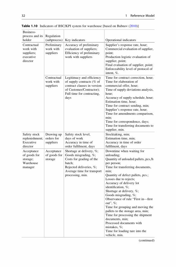
Table 1.10 Indicators of BSC/KPI system for warehouse [based on Bubnov (2010)]
Business-
process and its
holder
Regulation
(subprocess) Key indicators Operational indicators
Contractual
work with
suppliers;
executive
director
Preliminary
work with
suppliers
Accuracy of preliminary
evaluation of suppliers;
Efficiency of preliminary
work with suppliers
Supplier’s response rate, hour;
Commercial evaluation of supplier,
point;
Production logistic evaluation of
supplier, point;
Final evaluation of supplier, point;
Enforceability level of protocol of
intent, %.
Contractual
work with
suppliers
Legitimacy and efficiency
of supply contracts (% of
contract clauses in version
of Customer/Contractor);
Full time for contracting,
days
Time for contract correction, hour;
Time for elaboration of
commercial offer, hour;
Time of supply deviations analysis,
hour;
Accuracy of supply schedule, hour;
Estimation time, hour;
Time for contract sending, min;
Supplier’s response rate, hour;
Time for amendments comparison,
min;
Time for correspondence, days;
Time for transferring documents to
supplier, min.
Safety stock
replenishment;
Executive
director
Drawing up
orders for
suppliers
Safety stock level,
days of work
Accuracy in time of
order fulfilment, days
Stocktaking, min;
Estimation time, min;
Accuracy in time of order
fulfilment, days
Acceptance
of goods for
storage;
Warehouse
manager
Acceptance
of goods for
storage
Shortage at delivery, %;
Goods misgrading, %;
Costs for grading of the
batch;
Rejected deliveries, %;
Average time for transport
processing, min.
Downtime when waiting for
unloading;
Quantity of unloaded pallets, pcs./h
per person;
Time for transferring documents,
min;
Quantity of defect pallets, pcs.;
Losses due to rejects;
Accuracy of delivery lot
identification, %;
Shortage at delivery, %;
Goods misgrading, %;
Observance of rule “First in—first
out”, %;
Time for grouping and moving the
pallets to the storage area, min;
Time for processing the shipment
documents, min;
Processed documents with
mistakes, %;
Time for loading tare into the
vehicle, min.
(continued)
32 1 Reference Model

game in case of winning this amount is increased by the same amount and in loss it
is reduced to zero.
In the first example, the player is going to spend the available money for food,
which may be purchased for $10 as well (though in smaller amounts). In the second
example, assume that a player is full and prefers to spend the available money for a
movie ticket, which costs exactly $20.
It is obvious that in the first case the game is a serious threat to the player, as in
case of loss, he risks being without any money for food. In the second case, the
game is quite reasonable, because losing changes very little in the player’s life and
the possible gain allows having a good time. It appears that the difference in the
initial situation leads to different purposes in behaviour and different attitude to the
winning or losing, even if these values are the same in different cases.
In each of the examples two results are possible—winning I1 and losing I2, eachof which, as we have seen, has a different value in different cases. The measure of
this value is called “utility”. It is known that under some rather general conditions
each expected result of possible action I corresponds to a certain number u(I) calledas utility of action I. Set of numbers u(I) forms a utility function characterized by
two important properties.
• First property of utility function.
u I1ð Þ > u I2ð Þ then and only then, when a person making a decision prefers I1,but not I2.
• Second property of utility function.
If I is an expected result of possible actions, moreover which with probability
P this expected result will be I1, with probability 1� P it will be I2, then
uðIÞ ¼ PuðI1Þ þ ð1� PÞuðI2Þ: ð1:2Þ
Table 1.10 (continued)
Business-
process and its
holder
Regulation
(subprocess) Key indicators Operational indicators
Placement
of goods
in the
warehouse
Observance of rule “First
in—first out”, %;
Expired goods batches in
the storage area;
Loss due to goods returned;
Loss due to incorrect
placement;
Average time for moving
one pallet, min.
Incorrect placement of pallets, %;
Time for moving faulty goods to
the rejected area, min.;
Accuracy in moving the pallets, %;
Average time for moving one
pallet to storage area, min;
Time for execution of certificate
of unserviceability, min;
Write-off of goods due to return
and natural loss, %;
Time for moving from the rejected
area to waste container, min.
1.7 Utility of Quality Parameters 33

1.7.2 Typical Utility Functions
Figure 1.12 shows a diagram of the utility function, which Chernoff and Moses
(1959) call as function of Campbell. Along the horizontal axis in this figure the
value of capital in some units is plotted. The capital is available for either Campbell
or may be formed by the actions of the latter. Ordinates of the utility value of this
capital are determined according to the representations of Campbell depending on
its current amount, and the combination of these ordinates forms the diagram of
utility function. The diagram in Fig. 1.12 makes it possible to analyse different
cases of actions of a decision maker in different situations and assess their
reasonability.
Suppose that in the initial state Campbell has a capital of 8 units and this capital
corresponds to utility equal to 1. We consider two variants of the game with
different conditions. In the first case, the variant in terms of which with probability
0.5 you can win 2 units and just as likely to lose 1 unit. Apparently, this game can be
favourable for Campbell. Indeed, since the amount of capital in the event of
winning will be equal to 10 units, the utility according to the diagram in Fig. 1.12
will be equal to 1.18. In case of loss, the capital decreases to 7 units and the utility
will be equal to 0.86. Using formula (1.2), we obtain
1.6
1.5
1.4
1.3
1.2
1.1
0.9
0.8
0.7
0.6
0.5
0.4
0.3
0.2
0.1
00 1 2 3 4 5 6 7 8
Capital S
Uti
lity
U
9 10 11 12 13 14 15
1
Fig. 1.12 Utility function of Campbell
34 1 Reference Model
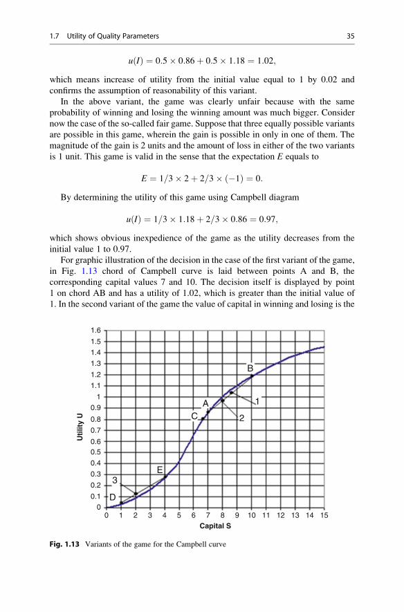
u Ið Þ ¼ 0:5� 0:86þ 0:5� 1:18 ¼ 1:02;
which means increase of utility from the initial value equal to 1 by 0.02 and
confirms the assumption of reasonability of this variant.
In the above variant, the game was clearly unfair because with the same
probability of winning and losing the winning amount was much bigger. Consider
now the case of the so-called fair game. Suppose that three equally possible variants
are possible in this game, wherein the gain is possible in only in one of them. The
magnitude of the gain is 2 units and the amount of loss in either of the two variants
is 1 unit. This game is valid in the sense that the expectation E equals to
E ¼ 1=3� 2þ 2=3� �1ð Þ ¼ 0:
By determining the utility of this game using Campbell diagram
u Ið Þ ¼ 1=3� 1:18þ 2=3� 0:86 ¼ 0:97;
which shows obvious inexpedience of the game as the utility decreases from the
initial value 1 to 0.97.
For graphic illustration of the decision in the case of the first variant of the game,
in Fig. 1.13 chord of Campbell curve is laid between points A and B, the
corresponding capital values 7 and 10. The decision itself is displayed by point
1 on chord AB and has a utility of 1.02, which is greater than the initial value of
1. In the second variant of the game the value of capital in winning and losing is the
1.6
1.5
1.4
1.3
1.2
1.1
0.9
0.8
0.7
0.60.5
0.4
0.3
0.23
D
E
CA
B
2
1
0.1
00 1 2 3 4 5 6 7 8
Capital S
Uti
lity
U
9 10 11 12 13 14 15
1
Fig. 1.13 Variants of the game for the Campbell curve
1.7 Utility of Quality Parameters 35
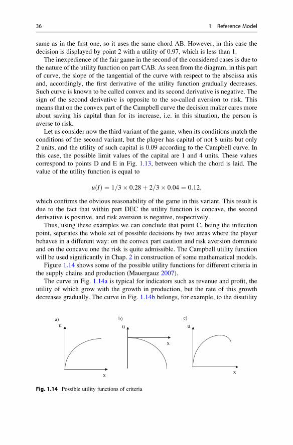
same as in the first one, so it uses the same chord AB. However, in this case the
decision is displayed by point 2 with a utility of 0.97, which is less than 1.
The inexpedience of the fair game in the second of the considered cases is due to
the nature of the utility function on part CAB. As seen from the diagram, in this part
of curve, the slope of the tangential of the curve with respect to the abscissa axis
and, accordingly, the first derivative of the utility function gradually decreases.
Such curve is known to be called convex and its second derivative is negative. The
sign of the second derivative is opposite to the so-called aversion to risk. This
means that on the convex part of the Campbell curve the decision maker cares more
about saving his capital than for its increase, i.e. in this situation, the person is
averse to risk.
Let us consider now the third variant of the game, when its conditions match the
conditions of the second variant, but the player has capital of not 8 units but only
2 units, and the utility of such capital is 0.09 according to the Campbell curve. In
this case, the possible limit values of the capital are 1 and 4 units. These values
correspond to points D and E in Fig. 1.13, between which the chord is laid. The
value of the utility function is equal to
u Ið Þ ¼ 1=3� 0:28þ 2=3� 0:04 ¼ 0:12;
which confirms the obvious reasonability of the game in this variant. This result is
due to the fact that within part DEC the utility function is concave, the second
derivative is positive, and risk aversion is negative, respectively.
Thus, using these examples we can conclude that point C, being the inflection
point, separates the whole set of possible decisions by two areas where the player
behaves in a different way: on the convex part caution and risk aversion dominate
and on the concave one the risk is quite admissible. The Campbell utility function
will be used significantly in Chap. 2 in construction of some mathematical models.
Figure 1.14 shows some of the possible utility functions for different criteria in
the supply chains and production (Mauergauz 2007).
The curve in Fig. 1.14a is typical for indicators such as revenue and profit, the
utility of which grow with the growth in production, but the rate of this growth
decreases gradually. The curve in Fig. 1.14b belongs, for example, to the disutility
x
x
x
u u ua) b) c)
Fig. 1.14 Possible utility functions of criteria
36 1 Reference Model

of necessary current assets, which with increasing volumes cannot just grow, but
grow with increasing speed.
Both of these curves are monotonically changing; alternatively to them, the
curve on Fig. 1.14c is not monotonic, i.e. its utility increases to a certain value of the
abscissa and then starts decreasing. This situation is typical for equipment load
criteria, which usually has the best value not at full load but at a lesser value. Note
that all the curves in Fig. 1.14 have a negative second derivative and, accordingly, a
positive risk aversion.
1.7.3 Utility Functions in Business Process Quality Evaluations
Each of the utility functions, presented in Sect. 1.7.2, describes the change in the
utility of one variable—profit, amounts of used current assets, machine utilization,
etc. These utility functions are called one dimensional. At the same time, as it
follows from the balanced scorecard described in Sect. 1.6.3, the objectives of the
enterprise are possible to achieve only with sufficiently high values of a set of
indicators, given in the strategic map, for example—Table 1.9. Although the
balanced scorecard allows determination of the set, but it does not define the
level of importance of an indicator or take into account the possible interaction
between the indicators.
To determine the joint effect of indicators set on the quality of the process under
consideration, it is obviously necessary:
• Construct the utility function for each indicator.
• With this function define the indicator’s utility by its current value.
• Using any method, establish the total utility of the existing values of the
indicators in this set.
The latter is possible, generally speaking, by any of the two methods. In the first
case, the utility of each indicator can be considered as an independent criterion and
for assessing their joint effect can use methods for solving multiobjective problems.
This method will be discussed further in Chap. 4. The second method is to construct
a multidimensional utility function, which is a certain combination of several
one-dimensional functions. An example using this method is given below.
The article of Youngblood and Collins (2003) describes the approach of the joint
study of the balanced scorecard (BSC) andMulti-Attribute Utility Theory (MAUT),
which includes four stages of the business process modelling. On the first stage,
BSC map is developed and measurable criteria are defined for each of the four
directions of BSC, as described above.
On the second stage, a description of one-dimensional utility functions for each
criterion is made. Besides, the lowest value of utility is deemed to be 0 and the
highest one is 1. On the utility curve, the lower and upper limits of admissible
1.7 Utility of Quality Parameters 37
values of utility are set. The convexity or concavity of the curve of utility, as
described above, determines the sign of risk aversion. The utility function having
the form of a straight line has zero risk aversion.
On the third stage, the criteria are ranked in order of importance and the weight
of each criterion among the criteria in this direction is set as a percentage. The sum
of these weights should be equal to 100 %. The range of possible values for each
criterion, with which this criterion is independent of other criteria, is determined.
Utility functions of several independent criteria can be combined into one group
considering the weight of each factor, forming the so-called additive utility func-
tion. If the criteria are dependent on each other, their utility functions are multiplied
together to form the so-called multiplicative function.
On the last, fourth stage of the study the BSC map is reviewed for compliance of
the numerical description of the business process utility with the ideas of a decision
maker, which play different scenarios of changes in the business process. If
necessary, some adjustments are performed on utility functions and maps in
general. The resulting map is called Utility-based Balanced Scorecard (UBSC).
In the paper of Youngblood et al. (2004), the mentioned approach is illustrated
by a practical example. This study examines the production activities of one of the
branches of a large company involved in the wholesale trade all over the world with
the nomenclature of approximately 500,000 items. With this nomenclature, this
department performs nearly 25 million transactions a year.
Table 1.11 shows UBSC map, including data on the criteria utility, their impact
in all directions, and the importance of these directions. Department management
believes that business processes are the most important direction, so for this group
of criteria the greatest weighting factor is set equal to 33 %. The financial direction
with a weighting factor of 27 % is the second in importance. In both groups, the
weighting factor is the same and equals to 20 % in each group. For the first three
directions, all indicators and their parameters are listed in Table 1.11 and for the
latter group only general data of the group as a whole is given. The meaning of each
of the indicators is generally clear from their names; the quantity of the current
value was determined at the time of the study.
The values of the entries in columns 3–7 of Table 1.11 reflect the character of
relevant utility function, where the value of index “insufficient” corresponds to
utility value equal to 0. When the index values equal to “below average”, “aver-
age”, “above average”, the utility takes values of 0.25, 0.5 and 0.75, respectively.
Utility is equal to 1 for the “best” values of the index. The current value of the utility
matches the current value of the index. Figure 1.15 presents two examples of utility
functions for indicators of Table 1.11.
Each of the utility curves in Fig. 1.15 has three parts: a part with 0 utility, a part
with utility equal to 1, and the actual utility curve between these two parts.
The utility of the average price deviation from the basic values (Fig. 1.15a)
increases linearly with decreasing prices and reaches one in the case price decrease
by 10 %. Point K marks the current state of the system, the utility of which is close
38 1 Reference Model
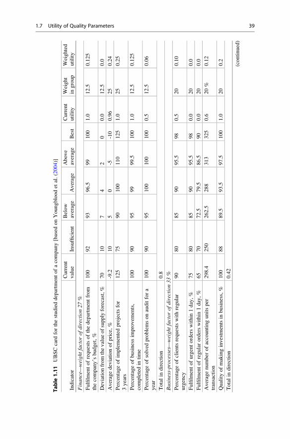
Table
1.11
UBSCcard
forthestudieddepartm
entofacompany[based
onYoungbloodet
al.(2004)]
Indicator
Current
value
Insufficient
Below
average
Average
Above
average
Best
Current
utility
Weight
ingroup
Weighted
utility
Finance—
weightfactor
ofdirection27
%
Fulfilm
entofrequestsofthedepartm
entfrom
thecompany’sbudget,%
100
92
93
96.5
99
100
1.0
12.5
0.125
Deviationfromthevalueofsupply
forecast,%
70
10
74
20
0.0
12.5
0.0
Averagedeviationofprice,%
-9.2
10
50
-5-10
0.96
25
0.24
Percentageofim
plementedprojectsfor
3years
125
75
90
100
110
125
1.0
25
0.25
Percentageofbusinessim
provem
ents,
completedin
time
100
90
95
99
99.5
100
1.0
12.5
0.125
Percentageofsolved
problemsonauditfora
year
100
90
95
100
100
100
0.5
12.5
0.06
Totalin
direction
0.8
Business-processes—weight
factorof
direction33
%
Percentageofclientsrequestswithregular
urgency
90
80
85
90
95.5
98
0.5
20
0.10
Fulfilm
entofurgentorderswithin
1day,%
75
80
85
90
95.5
98
0.0
20
0.0
Fulfilm
entofregularorderswithin
1day,%
65
70
72.5
79.5
86.5
90
0.0
20
0.0
Averagenumber
ofaccountingunitsper
transaction
298.4
250
262.5
288
313
325
0.6
20%
0.12
Qualityofmakinginvestm
entsin
business,%
100
88
89.5
93.5
97.5
100
1.0
20
0.2
Totalin
direction
0.42
(continued)
1.7 Utility of Quality Parameters 39
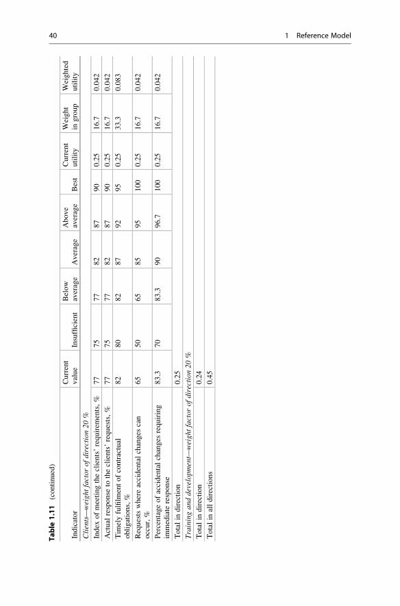
Table
1.11
(continued)
Indicator
Current
value
Insufficient
Below
average
Average
Above
average
Best
Current
utility
Weight
ingroup
Weighted
utility
Clients—weigh
tfactorof
direction
20%
Index
ofmeetingtheclients’requirem
ents,%
77
75
77
82
87
90
0.25
16.7
0.042
Actual
response
totheclients’requests,%
77
75
77
82
87
90
0.25
16.7
0.042
Tim
elyfulfilm
entofcontractual
obligations,%
82
80
82
87
92
95
0.25
33.3
0.083
Requestswhereaccidentalchanges
can
occur,%
65
50
65
85
95
100
0.25
16.7
0.042
Percentageofaccidentalchanges
requiring
immediate
response
83.3
70
83.3
90
96.7
100
0.25
16.7
0.042
Totalin
direction
0.25
Trainingan
ddevelopment—
weight
factor
ofdirection20
%
Totalin
direction
0.24
Totalin
alldirections
0.45
40 1 Reference Model
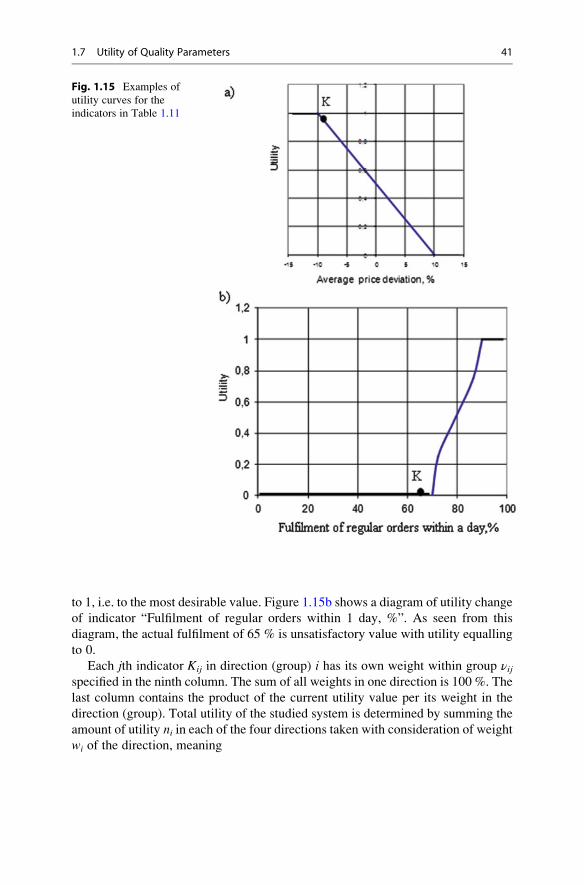
to 1, i.e. to the most desirable value. Figure 1.15b shows a diagram of utility change
of indicator “Fulfilment of regular orders within 1 day, %”. As seen from this
diagram, the actual fulfilment of 65 % is unsatisfactory value with utility equalling
to 0.
Each jth indicator Kij in direction (group) i has its own weight within group νijspecified in the ninth column. The sum of all weights in one direction is 100 %. The
last column contains the product of the current utility value per its weight in the
direction (group). Total utility of the studied system is determined by summing the
amount of utility ni in each of the four directions taken with consideration of weightwi of the direction, meaning
Fig. 1.15 Examples of
utility curves for the
indicators in Table 1.11
1.7 Utility of Quality Parameters 41
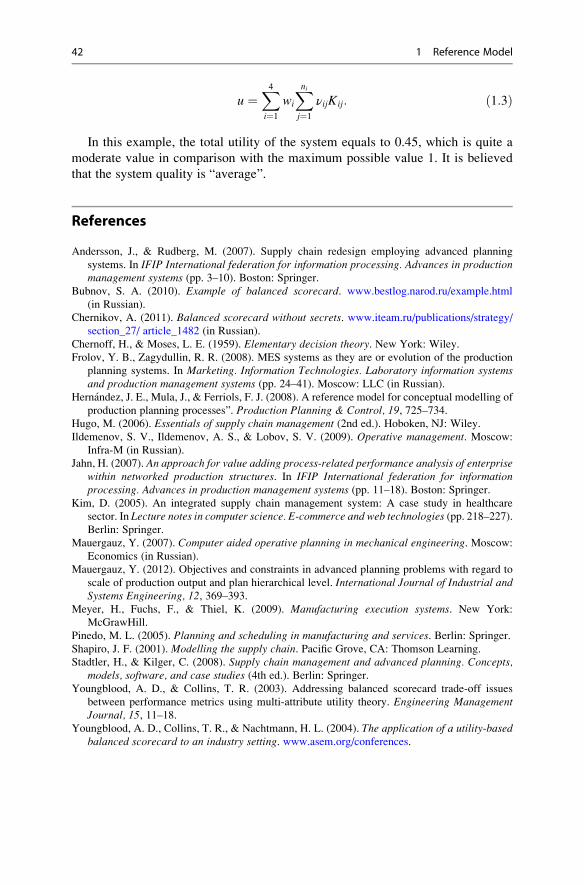
u ¼X4i¼1
wi
Xnij¼1
νijKij: ð1:3Þ
In this example, the total utility of the system equals to 0.45, which is quite a
moderate value in comparison with the maximum possible value 1. It is believed
that the system quality is “average”.
References
Andersson, J., & Rudberg, M. (2007). Supply chain redesign employing advanced planning
systems. In IFIP International federation for information processing. Advances in productionmanagement systems (pp. 3–10). Boston: Springer.
Bubnov, S. A. (2010). Example of balanced scorecard. www.bestlog.narod.ru/example.html
(in Russian).
Chernikov, A. (2011). Balanced scorecard without secrets. www.iteam.ru/publications/strategy/
section_27/ article_1482 (in Russian).
Chernoff, H., & Moses, L. E. (1959). Elementary decision theory. New York: Wiley.
Frolov, Y. B., Zagydullin, R. R. (2008). MES systems as they are or evolution of the production
planning systems. In Marketing. Information Technologies. Laboratory information systemsand production management systems (pp. 24–41). Moscow: LLC (in Russian).
Hernandez, J. E., Mula, J., & Ferriols, F. J. (2008). A reference model for conceptual modelling of
production planning processes”. Production Planning & Control, 19, 725–734.Hugo, M. (2006). Essentials of supply chain management (2nd ed.). Hoboken, NJ: Wiley.
Ildemenov, S. V., Ildemenov, A. S., & Lobov, S. V. (2009). Operative management. Moscow:
Infra-M (in Russian).
Jahn, H. (2007). An approach for value adding process-related performance analysis of enterprisewithin networked production structures. In IFIP International federation for informationprocessing. Advances in production management systems (pp. 11–18). Boston: Springer.
Kim, D. (2005). An integrated supply chain management system: A case study in healthcare
sector. In Lecture notes in computer science. E-commerce and web technologies (pp. 218–227).Berlin: Springer.
Mauergauz, Y. (2007). Computer aided operative planning in mechanical engineering. Moscow:
Economics (in Russian).
Mauergauz, Y. (2012). Objectives and constraints in advanced planning problems with regard to
scale of production output and plan hierarchical level. International Journal of Industrial andSystems Engineering, 12, 369–393.
Meyer, H., Fuchs, F., & Thiel, K. (2009). Manufacturing execution systems. New York:
McGrawHill.
Pinedo, M. L. (2005). Planning and scheduling in manufacturing and services. Berlin: Springer.Shapiro, J. F. (2001). Modelling the supply chain. Pacific Grove, CA: Thomson Learning.
Stadtler, H., & Kilger, C. (2008). Supply chain management and advanced planning. Concepts,models, software, and case studies (4th ed.). Berlin: Springer.
Youngblood, A. D., & Collins, T. R. (2003). Addressing balanced scorecard trade-off issues
between performance metrics using multi-attribute utility theory. Engineering ManagementJournal, 15, 11–18.
Youngblood, A. D., Collins, T. R., & Nachtmann, H. L. (2004). The application of a utility-basedbalanced scorecard to an industry setting. www.asem.org/conferences.
42 1 Reference Model
Mathematical Models 2
2.1 Simplest Planning Models
Generally, production and supply chain planning shall provide answers to the
following three main questions:
• What products will we need?
• How much of each product will we need?
• When will we need this?
As a general matter, this is quite difficult to give answers to these questions in the
current market environment. Actually, all methods, techniques, and solutions
described herein have been developed exactly for this purpose. However, they do
not provide a fully exhaustive and comprehensive solution to this challenge.
Complexity and sometimes the whole possibility of a planning task depend on the
complexity of a certain production situation. Therefore, it is methodologically
practical to consider various task cases in the ascending order of complexity. So,
we shall start with the simplest mathematical model (described in Sect. 2.1.1).
2.1.1 Classical Supply Management Model
Let us consider a warehouse where a certain product is accepted, stored, and
gradually issued to consumers. Figure 2.1 shows the time plot of the product
quantity changes.
According to this plot, the product in the quantity Q is delivered to the ware-
house at a constant time frequency T which exactly equals the time of consumption
of the accepted product batch, i.e.
# Springer International Publishing Switzerland 2016
Y. Mauergauz, Advanced Planning and Scheduling in Manufacturing and SupplyChains, DOI 10.1007/978-3-319-27523-9_2
43
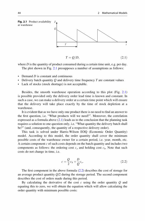
T ¼ Q=D; ð2:1ÞwhereD is the quantity of product consumed during a certain time unit, e.g. per day.
The plot shown in Fig. 2.1 presupposes a number of assumptions as follows:
• Demand D is constant and continuous
• Delivery batch quantity Q and delivery time frequency T are constant values
• Lack of stocks (stock shortage) is not acceptable.
Besides, the smooth warehouse operation according to this plot (Fig. 2.1)
is possible provided only the delivery order lead time is known and constant. In
such a case, we can make a delivery order at a certain time point which will ensure
that the delivery will take place exactly by the time of stock depletion at a
warehouse.
It is evident that as we have only one product there is no need to find an answer to
the first question, i.e. “What products will we need?”. Moreover, the correlation
expressed as a formula above (2.1) leads us to the conclusion that the planning task
requires a solution to one question only, i.e. “What quantity the delivery batch shall
be?” (and, consequently, the quantity of a respective delivery order).
This task is solved under Harris-Wilson EOQ (Economic Order Quantity)
model. According to this model, the order quantity shall cover the minimum
possible costs of the warehouse owner for a certain period, i.e. year, month, etc.
A certain component c of such costs depends on the batch quantity and includes twocomponents as follows: the ordering cost co and holding cost ch. Note that such
costs do not change in time, i.e.
c ¼ Q
2ch þ D
Qco: ð2:2Þ
The first component in the above formula (2.2) describes the cost of storage for
an average product quantity Q/2 during the storage period. The second component
describes the cost of orders made during this period.
By calculating the derivative of the cost c using the order quantity Q and
equating this to zero, we will obtain the equation which will allow calculating the
order quantity with minimum possible costs:
Z
Q
tT
Fig. 2.1 Product availability
at warehouse
44 2 Mathematical Models
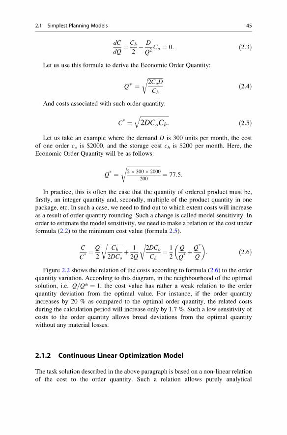
dC
dQ¼ Ch
2� D
Q2Co ¼ 0: ð2:3Þ
Let us use this formula to derive the Economic Order Quantity:
Q∗ ¼ffiffiffiffiffiffiffiffiffiffiffi2CoD
Ch
rð2:4Þ
And costs associated with such order quantity:
C* ¼ffiffiffiffiffiffiffiffiffiffiffiffiffiffiffiffiffiffiffiffiffi2DCoCh:
qð2:5Þ
Let us take an example where the demand D is 300 units per month, the cost
of one order co is $2000, and the storage cost ch is $200 per month. Here, the
Economic Order Quantity will be as follows:
Q* ¼ffiffiffiffiffiffiffiffiffiffiffiffiffiffiffiffiffiffiffiffiffiffiffiffiffi2� 300� 2000
200
r¼ 77:5:
In practice, this is often the case that the quantity of ordered product must be,
firstly, an integer quantity and, secondly, multiple of the product quantity in one
package, etc. In such a case, we need to find out to which extent costs will increase
as a result of order quantity rounding. Such a change is called model sensitivity. In
order to estimate the model sensitivity, we need to make a relation of the cost under
formula (2.2) to the minimum cost value (formula 2.5).
C
C*¼ Q
2
ffiffiffiffiffiffiffiffiffiffiffiCh
2DCo
rþ 1
2Q
ffiffiffiffiffiffiffiffiffiffiffi2DCo
Ch
r¼ 1
2
Q
Q*þ Q*
Q
� �: ð2:6Þ
Figure 2.2 shows the relation of the costs according to formula (2.6) to the order
quantity variation. According to this diagram, in the neighbourhood of the optimal
solution, i.e. Q=Q* ¼ 1, the cost value has rather a weak relation to the order
quantity deviation from the optimal value. For instance, if the order quantity
increases by 20 % as compared to the optimal order quantity, the related costs
during the calculation period will increase only by 1.7 %. Such a low sensitivity of
costs to the order quantity allows broad deviations from the optimal quantity
without any material losses.
2.1.2 Continuous Linear Optimization Model
The task solution described in the above paragraph is based on a non-linear relation
of the cost to the order quantity. Such a relation allows purely analytical
2.1 Simplest Planning Models 45
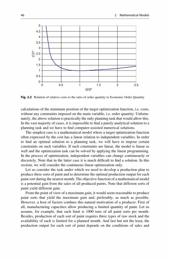
calculations of the minimum position of the target optimization function, i.e. costs,
without any constraints imposed on the main variable, i.e. order quantity. Unfortu-
nately, the above solution is practically the only planning task that would allow this.
In the vast majority of cases, it is impossible to find a purely analytical solution to a
planning task and we have to find computer-assisted numerical solutions.
The simplest case is a mathematical model where a target optimization function
often expressed by the cost has a linear relation to independent variables. In order
to find an optimal solution to a planning task, we will have to impose certain
constraints on such variables. If such constraints are linear, the model is linear as
well and the optimization task can be solved by applying the linear programming.
In the process of optimization, independent variables can change continuously or
discretely. Note that in the latter case it is much difficult to find a solution. In this
section, we will consider the continuous linear optimization only.
Let us consider the task under which we need to develop a production plan to
produce three sorts of paint and to determine the optimal production output for each
paint sort during the nearest month. The objective function of a mathematical model
is a potential gain from the sales of all produced paints. Note that different sorts of
paint yield different gain.
From the point of view of a maximum gain, it would seem reasonable to produce
paint sorts that yield the maximum gain and, preferably, as much as possible.
However, a host of factors confines this natural motivation of a producer. First of
all, manufacturing capacities allow producing a limited quantity of paint. Let us
assume, for example, that such limit is 1000 tons of all paint sorts per month.
Besides, production of each sort of paint requires three types of raw stock and the
availability of each is limited for a planned month. And last but not the least, the
production output for each sort of paint depends on the conditions of sales and
5
4.5
3.5
4
2.5
3
1.5
2
0.5
1
00 0.5 1
Q/Q*
C/C
*
1.5 2 2.5
Fig. 2.2 Relation of relative costs to the ratio of order quantity to Economic Order Quantity
46 2 Mathematical Models
marketing. Generally, only small quantities of expensive paint are sold, while
cheaper paints can be pre-ordered, etc.
The product parameters and constraints are described in Table 2.1, and raw stock
constraints are shown in Table 2.2. The quantity of a water-based is paint assumed
unlimited.
Using Tables 2.1 and 2.2, we can create a mathematical model which shall
contain three basic components as follows:
• Variables whose values need to be calculated, i.e. find solutions to the task
• Objective function whose value depends on the values of the variables
(indicating the solution objective, i.e. minimum or maximum)
• Task constraints expressed as mathematical inequalities (or equalities).
Let us set x1, x2, and x3 as variables that determine monthly production outputs for
paint sort No. 1, No. 2, and No. 3, respectively. Using gain values from Table 2.1, we
will obtain the expression for the objective function, i.e. cumulative gain.
f xð Þ ¼ 200x1 þ 280x2 þ 250x3; ð2:7Þwhich shall be maximized.
According to Tables 2.1 and 2.2, the mathematical model provides for a host of
constraints as follows:
Production capacity constraint:
x1 þ x2 þ x3 � 1000: ð2:8Þ
Table 2.1 Product parameters and constraints
Parameter Paint no. 1 Paint no. 2 Paint no. 3
Gain, dollars per ton 200 280 250
Quantity of raw stock 1, kg per ton 150 220 170
Quantity of raw stock 2, kg per ton 80 70 100
Quantity of raw stock 3, kg per ton 100 80 90
Minimum number of tons per month 400 – –
Maximum number of tons per month – 200 –
Table 2.2 Raw stock constraints
Parameter Value
The maximum possible cumulative production output for all paint sorts, tons per month 1000
The maximum possible consumption of raw stock 1, tons per month 160
The maximum possible consumption of raw stock 2, tons per month 70
The maximum possible consumption of raw stock 3, tons per month 70
2.1 Simplest Planning Models 47

Marketing constraints:
x1 � 400; x2 � 200: ð2:9ÞRaw stock consumption constraints:
0:15x1 þ 0:22x2 þ 0:17x3 � 160;0:08x1 þ 0:07x2 þ 0:1x3 � 70;0:1x1 þ 0:08x2 þ 0:09x3 � 70:
ð2:10Þ
Another implicit constraint is that variables of paint production outputs shall be
non-negative, i.e.:
x1 � 0; x2 � 0; x3 � 0: ð2:11ÞThe first of these conditions (2.11) is actually redundant as it is overlapped by a
stronger condition (2.9). Therefore, only two conditions from (2.11) remain in
force:
x2 � 0; x3 � 0: ð2:12ÞThe resulting mathematical model is somewhat more complicated than the
model described in Sect. 2.1.1 above as it takes account of planning for multiple
products rather than one product. However, here as well, types of produced
products are pre-set rather than determined during planning. And the most impor-
tant thing is that this mathematical model does not determine the production
sequence for such types. Similarly to the model described in Sect. 2.1.1, this
model takes into account only the quantities of products planned for production
in a respective planned period and disregards the production details. Therefore, this
task can also be deemed as simplest.
Expressions (2.7)–(2.10) and (2.12) describing the created mathematical model
show that each expression contain first-degree variables, i.e. the mathematical
model is linear to the variables. As mentioned above, a solution is found using
any method of linear programming. It is practically feasible to use MS Excel which
has respective built-in methods. Figure 2.3 shows the solution to the example task.
The upper part of MS Excel table shown in Fig. 2.3 contains randomly selected
input values of task variables. They are followed by coefficients of the objective
function; then, the input value of the objective function is calculated based on
expression (2.7).
Lines 11–17 list all the constraints imposed on the variables according to
inequalities (2.8)–(2.10) and (2.12). Such constraints are grouped by the correlations
of the left-hand and right-hand sides of the inequalities. Line 20 shows variable
values and the resulting value of gain for an optimal solution. The solution is found
by initiating the Solver add-in for a continuous linear optimization case.
48 2 Mathematical Models
If we compare the resulting gain value shown in E20 cell with the input value
in E8 cell, we will see that the optimal solution provides for a substantial gain
increase. However, this solution is calculated under a host of imposed constraints
and this poses a question to which extent the optimal solution depends on the values
of such constraints. First of all, we need to determine which constraints are material
for this task.
Constraints shall be deemed material or coupled if their left-hand values equal
to right-hand values under an optimal solution. In Fig. 2.3, there are three
coupled constraints, i.e. two marketing constraints and one raw stock 3 constraint.
Production capacity constraint is not coupled and this actually means under-
utilization of available production capacities. Naturally, in order to evaluate the
quality of a found solution and the viability of any changes, we need to analyse
sensitivity of such solution (somewhat similar to sensitivity analysis as described in
Sect. 2.1.1).
A more detailed sensitivity analysis may provide answers to the following
questions:
Fig. 2.3 Solving a continuous linear optimization task using MS Excel
2.1 Simplest Planning Models 49
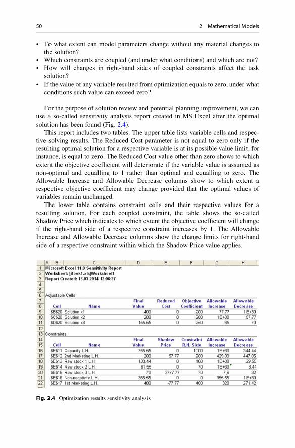
• To what extent can model parameters change without any material changes to
the solution?
• Which constraints are coupled (and under what conditions) and which are not?
• How will changes in right-hand sides of coupled constraints affect the task
solution?
• If the value of any variable resulted from optimization equals to zero, under what
conditions such value can exceed zero?
For the purpose of solution review and potential planning improvement, we can
use a so-called sensitivity analysis report created in MS Excel after the optimal
solution has been found (Fig. 2.4).
This report includes two tables. The upper table lists variable cells and respec-
tive solving results. The Reduced Cost parameter is not equal to zero only if the
resulting optimal solution for a respective variable is at its possible value limit, for
instance, is equal to zero. The Reduced Cost value other than zero shows to which
extent the objective coefficient will deteriorate if the variable value is assumed as
non-optimal and equalling to 1 rather than optimal and equalling to zero. The
Allowable Increase and Allowable Decrease columns show to which extent a
respective objective coefficient may change provided that the optimal values of
variables remain unchanged.
The lower table contains constraint cells and their respective values for a
resulting solution. For each coupled constraint, the table shows the so-called
Shadow Price which indicates to which extent the objective coefficient will change
if the right-hand side of a respective constraint increases by 1. The Allowable
Increase and Allowable Decrease columns show the change limits for right-hand
side of a respective constraint within which the Shadow Price value applies.
Fig. 2.4 Optimization results sensitivity analysis
50 2 Mathematical Models
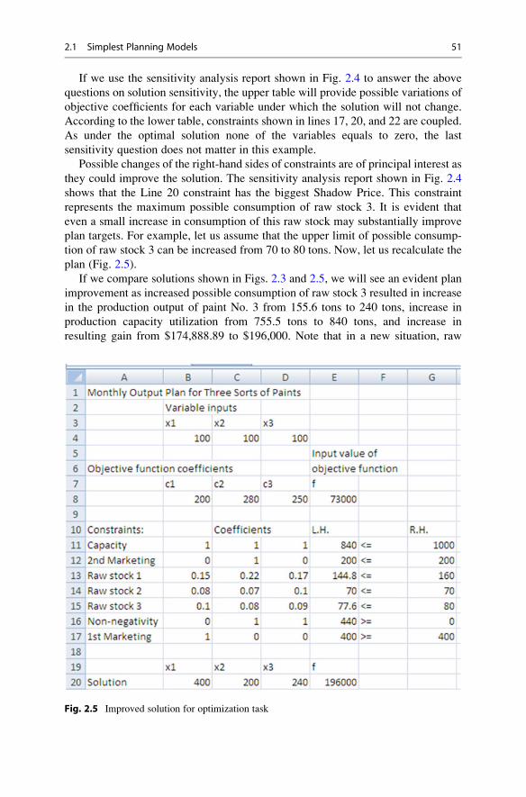
If we use the sensitivity analysis report shown in Fig. 2.4 to answer the above
questions on solution sensitivity, the upper table will provide possible variations of
objective coefficients for each variable under which the solution will not change.
According to the lower table, constraints shown in lines 17, 20, and 22 are coupled.
As under the optimal solution none of the variables equals to zero, the last
sensitivity question does not matter in this example.
Possible changes of the right-hand sides of constraints are of principal interest as
they could improve the solution. The sensitivity analysis report shown in Fig. 2.4
shows that the Line 20 constraint has the biggest Shadow Price. This constraint
represents the maximum possible consumption of raw stock 3. It is evident that
even a small increase in consumption of this raw stock may substantially improve
plan targets. For example, let us assume that the upper limit of possible consump-
tion of raw stock 3 can be increased from 70 to 80 tons. Now, let us recalculate the
plan (Fig. 2.5).
If we compare solutions shown in Figs. 2.3 and 2.5, we will see an evident plan
improvement as increased possible consumption of raw stock 3 resulted in increase
in the production output of paint No. 3 from 155.6 tons to 240 tons, increase in
production capacity utilization from 755.5 tons to 840 tons, and increase in
resulting gain from $174,888.89 to $196,000. Note that in a new situation, raw
Fig. 2.5 Improved solution for optimization task
2.1 Simplest Planning Models 51
stock 3 constraint is not coupled anymore and does not limit further production
while raw stock 2 constraint becomes coupled. Naturally, for further production
plan improvements we should increase consumption of raw stock 2 instead of
further consumption increase for raw stock 3.
2.2 Correlations Between Mathematical and ReferenceModels
The example described in Sect. 2.1.2 demonstrated how it was possible to solve a
planning task with a preset objective function (gain) and known constraints on
resources and marketing. It is evident that when creating any other mathematical
planning model we need, first of all, to determine what plan parameter (criterion)
should be taken as an objective function. Other parameters can be taken as
constraints.
2.2.1 Main Criteria and Constraints
According to Kiran and Smith (1984), all criteria that can be used as an objective
function may be classified as follows based on the following planning parameters:
1. Process parameters including:
(a) Planned work completion time
(b) Work-in-process
(c) Capacity load
2. Order completion dates as contractually established
3. Production costs
On the other hand, as mentioned in Sect. 1.6.1, according to SCOR model,
planning quality criteria shall belong to one of the main categories, i.e. consumer
service level or cost-effectiveness. Under this approach, we can assume that criteria
based on such parameters as due dates and plan completion dates ensure a high
service level, while other criteria determine cost-effectiveness of production.
Below is a non-exhaustive list of potential optimization criteria and main
constraints (Table 2.3).
First two criteria shown in Table 2.3 evaluate, directly or indirectly, the level of
customer service; last three parameters are constraints, while others represent
various factors of cost-effectiveness. In addition to three main constraints as
shown in Table 2.3, certain task may impose on the mathematical model other
constraining conditions that can be related, for instance, with batch quantities, batch
sequence, and possible breaks during processing, etc.
52 2 Mathematical Models
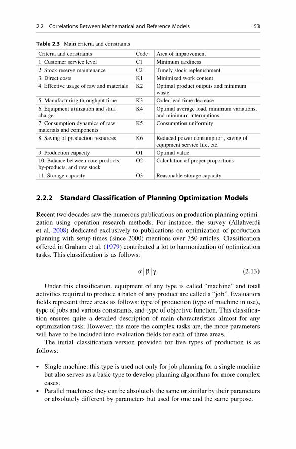
2.2.2 Standard Classification of Planning Optimization Models
Recent two decades saw the numerous publications on production planning optimi-
zation using operation research methods. For instance, the survey (Allahverdi
et al. 2008) dedicated exclusively to publications on optimization of production
planning with setup times (since 2000) mentions over 350 articles. Classification
offered in Graham et al. (1979) contributed a lot to harmonization of optimization
tasks. This classification is as follows:
α��β ��γ: ð2:13Þ
Under this classification, equipment of any type is called “machine” and total
activities required to produce a batch of any product are called a “job”. Evaluation
fields represent three areas as follows: type of production (type of machine in use),
type of jobs and various constraints, and type of objective function. This classifica-
tion ensures quite a detailed description of main characteristics almost for any
optimization task. However, the more the complex tasks are, the more parameters
will have to be included into evaluation fields for each of three areas.
The initial classification version provided for five types of production is as
follows:
• Single machine: this type is used not only for job planning for a single machine
but also serves as a basic type to develop planning algorithms for more complex
cases.
• Parallel machines: they can be absolutely the same or similar by their parameters
or absolutely different by parameters but used for one and the same purpose.
Table 2.3 Main criteria and constraints
Criteria and constraints Code Area of improvement
1. Customer service level C1 Minimum tardiness
2. Stock reserve maintenance C2 Timely stock replenishment
3. Direct costs K1 Minimized work content
4. Effective usage of raw and materials K2 Optimal product outputs and minimum
waste
5. Manufacturing throughput time K3 Order lead time decrease
6. Equipment utilization and staff
charge
K4 Optimal average load, minimum variations,
and minimum interruptions
7. Consumption dynamics of raw
materials and components
K5 Consumption uniformity
8. Saving of production resources K6 Reduced power consumption, saving of
equipment service life, etc.
9. Production capacity O1 Optimal value
10. Balance between core products,
by-products, and raw stock
O2 Calculation of proper proportions
11. Storage capacity O3 Reasonable storage capacity
2.2 Correlations Between Mathematical and Reference Models 53
• Flowshop: machines are arranged according to the process sequence and all
operations of each job are completed in the same sequence. It is acceptable that
different machines and different jobs may have different processing times.
• Jobshop: different jobs can be arranged in any process sequence.
• Openshop: different operations of each job can be completed in any sequence.
The number of machines for a respective type of production is indicated in field
α.Field β contains constraints of different types and nature. First of all, there are
various types of constraints imposed on job start and end dates. This field can also
specify codes of constraints on job priority, possible breaks during processing,
required batch processing, activity sequence, etc. Refer to Appendix C for the
detailed list of constraint codes.
An objective function indicated in field γ of the standard classification generallyrepresents one of work time indicators as follows:
• The most popular criterion is the total time of completion of all planned jobs
Cmax (makespan). Cmax equals to the time interval from the job start (0 point)
according to the plan till the completion of the last job indicated in such plan. It
is clear that:
Cmax ¼ max Cið Þ; ð2:14Þwhere Ci is the time of completion of i-job.• Flow time Fmax determines the maximum length of i-job
Fmax ¼ max Fið Þ at Fi ¼ Ci � ri; ð2:15Þwhere ri (release date) is the time of start of i-job.• Tmax represents the maximum tardiness in completion of i-job, i.e.:
Tmax ¼ max Tið Þ at Ti ¼ max 0,Ci � dið Þ; ð2:16Þwhere di (due date) is the time of work completion as specified by the customer.
• Lateness Lmax represents the maximum deviation of i-job from the due date, i.e.:
Lmax ¼ max Lij jð Þ at Li ¼ Ci � di: ð2:17ÞOther planning criteria and their combinations can also be used as an objective
function. For instance, we can use the sum of tardiness on each job Ti withweight wi for all n jobs:
Tw ¼Xni
wiTi: ð2:18Þ
54 2 Mathematical Models
• Cost criterion f can apply either to gain or to costs. In the first case, the criterion
will be fmax, and in the latter case it isfmin. When the weighted cost of tardiness is
used as a criterion, the following value will be determined:
f w ¼Xni¼1
wiTici; ð2:19Þ
where ci is the cost of one day of tardiness.
Refer to Appendix C for some other criteria.
2.2.3 Production Scale and Plan Hierarchy in Classification
Any existing production features all factors shown in Table 2.3; however, extents of
their influence may be quite different. Therefore, different types of production as
described in Sect. 1.3.1 and different levels of planning will have different criteria
priorities (Mauergauz 2012).
The nature of production has different effects on the planning methods at
different levels of planning. The least influence is applied to the Plan of Sales and
Operations where the main quality criterion is a possible gain value. The production
type and planning strategy, i.e. “Make-to-stock” (MTS) or “Make-to-order”
(MTO), play the critical role for other plans.
You might think that the planning strategy is rigidly bound to the production
scale; however, this is not always the case. The planning strategy MTS can be used
even for small-scale production provided that there is a relatively stable demand for
products. If the composition of products can be customized for orders, the MTS
strategy will be modified into the “Assemble-to-orders” (ATO) strategy, but the
bulk of components will be “Make-to-stock”, anyway. The MTO planning strategy
is often used for large-scale production, especially at the lower level of planning.
Tables 2.4, 2.5, and 2.6 show the structure of planning in accordance with the
terminology used in ERP systems and respective indicators for various production
types as described in Sect. 1.3.1. Refer to Table 2.3 for codes of criteria and
constraints.
Tables 2.4–2.6 lead us to a number of conclusions as follows:
• Any production type and any planning strategy require a master and short-term
plans. In some cases, for instance, in case of single machine bulk manufacturing
or automated production line these plans can be combined. Generally, the
smaller the scale of production is, the more plans will be required to ensure
such production.
• Most frequently, the main criterion for a master plan is minimized direct costs
(K1) that include setup and storage costs, order delay penalties, personnel hiring/
firing costs, overtime payments, outsourcing and subcontracting costs, etc. In
2.2 Correlations Between Mathematical and Reference Models 55
Table 2.4 Planning structure and indicators: one-stage production
Planning level
Production
strategy
Main
objective
Additional
criteria Constraints
Type 1 (single machine)—bulk and large-scale manufacturing
Master production
scheduling
MTS K1 K2 O1, C2
MTO C1 O1, K2
Shop floor scheduling MTS K4 C2 O1, O3
MTO C1 K4
Type 1 (single machine)—batch and small-scale manufacturing
Master production
scheduling
MTS K1 C2 O1, K2
MTO C1 K1
Shop floor scheduling MTS K3 K1 O1, C2, K6,
O3
MTO C1 O1, K6
Type 2 (parallel machines)
Master production
scheduling
MTS K1 K4 O1, C2
MTO O1, C1
Shop floor scheduling MTS K4 C2 O1, O3
MTO C1 K4
Table 2.5 Planning structure and indicators: synchronized flowshop production
Planning level
Production
strategy
Main
objective
Additional
criteria Constraints
Type 3a (automated production line)
Master production scheduling (alias
shop floor scheduling)
MTS – – O1, C2
Type 3b (versatile transfer line with output of core product only)—discrete manufacturing
Master production scheduling MTS K1 – O1, C2
MTO – O1, C1
Shop floor scheduling MTS C2 K1 O1
MTO C1
Type 3c (versatile transfer line with output of core product and by-products)—processmanufacturing
Master production scheduling MTS K2 K1 O1, O2, C2
MTO C1 O1, O2, K2
Shop floor scheduling MTS K1 C2 O1, K2, O3
MTO C1 K1 O1
Type 3d (flexible assembly line)
Master production scheduling MTS K5 K1 O1, C2
MTO O1, C1
Shop floor scheduling MTS C2 – O1
MTO C1 –
56 2 Mathematical Models
some cases, the master plan optimization will require indirect costs as a main
criterion. For instance, effective use of raw stock (K2) will be the most important
criterion for process manufacturing (type 3c), while for assembly line (type 3d)
the main criterion will be even consumption of materials and components (K5).
For discrete manufacturing, the smaller scale of production is the more impor-
tant master plan optimization constraints will be. In some cases, such constraints
shall be considered as additional criteria rather than constraints.
• A batch and small-scale production will require material requirements planning
if products include at least two components. However, simplest types of products
are manufactured in quite a large scale only. The main criterion of material
requirements planning is minimized throughput time (K3). Since material
requirement planning is based on a master production planning, optimization
generally concerns only the batch quantity. Generally, the need for timely
production is the constraint of material requirements planning. In some cases,
such need may become top priority; in this case, minimized throughput time will
be used as an additional criterion.
• The smaller the scale of production is, the greater need for timely comple-
tion will be. This factor will gradually shift from constraints to criteria.
It will become the main criterion for short-term plans. In case of job-shop
manufacturing, the discipline of completion of orders transferred from the master
plan andmaterial requirements planwill become themain indicator of performance
of production shops no matter which production strategy is adopted.
Table 2.6 Planning structure and indicators: batch, small-scale, and unique manufacturing
Planning level
Production
strategy
Main
objective
Additional
criteria Constraints
Type 4 (cellular manufacturing)
Master production
scheduling
MTS K1 K4 O1, C2
MTO O1, C1
Material requirements
planning
MTS K3 K4 O1, C2
MTO O1, C1
Shop floor scheduling MTS K3 C2 O1, K4
MTO C1 K3
Type 5 (job-shop manufacturing)
Master production
scheduling
MTS K1 C2 O1, K4
MTO C1
Material requirements
planning
MTS K3 C2 O1, K1
MTO C1 K3
Shop floor scheduling MTS C1 K6 O1, K4
MTO
Type 6 (project manufacturing)
Master production
scheduling
MTO C1 K1 O1
Shop floor scheduling K4
2.2 Correlations Between Mathematical and Reference Models 57
• The smaller scale of production is and the more detailed planning is, the more
criteria and constraints shall be taken account for discrete manufacturing
planning.
In addition to the above main criteria and constraints, in practice, the industry-
specific production planning system shall take account of various additional
industry-specific parameters. For instance, the paper (Zagidullin 2010) lists
30 parameters specific for the machine building industry.
2.3 Priority Rules
As mentioned in Sect. 2.2.2, single machine schedule algorithms often serve as a
basis for scheduling in more complex cases. Therefore, it is extremely important to
establish rules to determine single machine job sequence. There are quite a number
of such rules that are called priority rules. For instance, the publication (Panwalkar
and Iskander 1977) describes over 100 priority rules divided into 5 groups as
follows:
• Simple rules that are based on information pertaining to a certain job,
i.e. established due date, processing time, number of operations, etc.
• Simple rule combinations under which the job queue is divided into parts to
which certain simple rules apply.
• Weighted priorities under which simple rules apply to each job given its
weighted index.
• More complex rules that use various combinations of simple rules and take
account of time-based changes in characteristics of certain jobs.
• Other rules used under specific circumstances.
Let us consider some simple and weighted priority rules.
2.3.1 Simple Rules
The first of simple rules is a classic queuing rule according to which i-job that
appeared first in a queue shall be performed first, i.e. whose start time ri is earlier.This rule is called FIFO (First In First Out). Despite the usual “fairness” of this rule,
sometimes an opposite LIFO (Last In First Out) rule can be applied according to
which a job that has just arrived shall be performed first. This is the case, for
instance, when a rejected item must be corrected as soon as possible, etc. Another
simple rule that is less common though absolutely natural is the rule of first-priority
completion of a job with the nearest due date di. This rule is called EDD (Earliest
Due Date). The above simple rules are actually based on a time parameter, i.e. job
start or end.
58 2 Mathematical Models
There are a number of simple rules that are based on processing time. Two
simplest rules of this kind include the SPT rule (Shortest Processing Time) and the
LPT rule (Longest Processing Time). Despite their opposite purposes, both rules
have certain scopes of application.
To illustrate the practicality of SPT rule, let us consider the case where three jobs
are completed on a single machine with the processing time parameters being
p1 ¼ 1, p2 ¼ 5, and p3 ¼ 8 h, respectively. It is clear that if we take the makespan
Cmax as a process optimization criterion, the sequence of planned jobs does not
matter; in any case, Cmax ¼ 14 h. However, if we take the mean flow time F as an
optimization criterion, its value will greatly depend on the job sequence. For
instance, at {3, 2, 1} order the production cycle of job 1 will be 8 h, the mean
flow time of job 2 will be 13 h, and that of job 3 will be 14 h. In such a case, the
mean flow time for three jobs will be:
F ¼ 8þ 13þ 14ð Þ=3 ¼ 11:67 h:
However, if the order is {1, 2, 3}, the mean flow time will be just:
F ¼ 1þ 6þ 14ð Þ=3 ¼ 7 h:
The LPT rule is useful, for example, to distribute jobs between several parallel
machines in order to reduce the makespan Cmax. In this situation Cmax greatly
depends on the job sequence as even load applied on all parallel machines ensures
the minimum Cmax value. It is much easier to achieve even load if each of the
parallel machines will first be used for the longest jobs and then perform less
prolonged jobs at vacating machines.
The SPT rule has a popular modification, i.e. the Weighted Shortest Processing
Time rule (WSPT). According to this rule, jobs are completed in the descending
order for wi/pi which represents the ratio of priority factor wi of i-job to its
processing time pi.According to the terminology introduced in Pinedo (2005), all the above rules
are static as they do not directly depend on the time point where the plan has to be
performed. Simple rules also include some time-dependant dynamic rules, for
example MST rule (Minimum Slack Time).
The slack time value for each i-job at the planning time t is calculated as
max di � pi � t, 0ð Þ, i.e. slack time exists if di � pi � t � 0; otherwise, it does not
exist. In this situation production shall start with the job whose slack time is the
closest to zero. If there are several jobs with zero slack time (this actually means
past due date), there is no way to determine the sequence of such jobs.
Another dynamic rule is the so-called Critical Ratio (CR). According to this rule,
production shall start with a job which has the minimum value of di � tð Þ=pi.Similar to the previous rule, CR equals to zero if di � t � 0.
Let us take an example of applying several simple priority rules to jobs shown in
Table 2.7.
2.3 Priority Rules 59
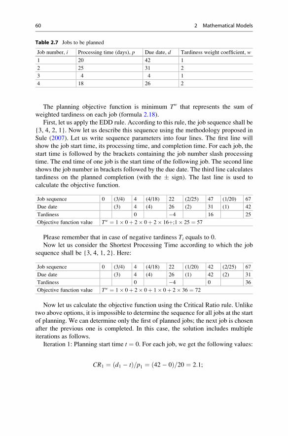
The planning objective function is minimum Tw that represents the sum of
weighted tardiness on each job (formula 2.18).
First, let us apply the EDD rule. According to this rule, the job sequence shall be
{3, 4, 2, 1}. Now let us describe this sequence using the methodology proposed in
Sule (2007). Let us write sequence parameters into four lines. The first line will
show the job start time, its processing time, and completion time. For each job, the
start time is followed by the brackets containing the job number slash processing
time. The end time of one job is the start time of the following job. The second line
shows the job number in brackets followed by the due date. The third line calculates
tardiness on the planned completion (with the � sign). The last line is used to
calculate the objective function.
Job sequence 0 (3/4) 4 (4/18) 22 (2/25) 47 (1/20) 67
Due date (3) 4 (4) 26 (2) 31 (1) 42
Tardiness 0 �4 16 25
Objective function value Tw ¼ 1� 0þ 2� 0þ 2� 16þ;1� 25 ¼ 57
Please remember that in case of negative tardiness Ti equals to 0.
Now let us consider the Shortest Processing Time according to which the job
sequence shall be {3, 4, 1, 2}. Here:
Job sequence 0 (3/4) 4 (4/18) 22 (1/20) 42 (2/25) 67
Due date (3) 4 (4) 26 (1) 42 (2) 31
Tardiness 0 �4 0 36
Objective function value Tw ¼ 1� 0þ 2� 0þ 1� 0þ 2� 36 ¼ 72
Now let us calculate the objective function using the Critical Ratio rule. Unlike
two above options, it is impossible to determine the sequence for all jobs at the start
of planning. We can determine only the first of planned jobs; the next job is chosen
after the previous one is completed. In this case, the solution includes multiple
iterations as follows.
Iteration 1: Planning start time t ¼ 0. For each job, we get the following values:
CR1 ¼ d1 � tð Þ=p1 ¼ 42� 0ð Þ=20 ¼ 2:1;
Table 2.7 Jobs to be planned
Job number, i Processing time (days), p Due date, d Tardiness weight coefficient, w
1 20 42 1
2 25 31 2
3 4 4 1
4 18 26 2
60 2 Mathematical Models
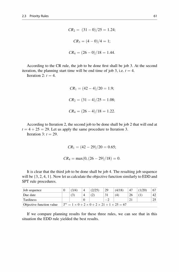
CR2 ¼ 31� 0ð Þ=25 ¼ 1:24;
CR3 ¼ 4� 0ð Þ=4 ¼ 1;
CR4 ¼ 26� 0ð Þ=18 ¼ 1:44:
According to the CR rule, the job to be done first shall be job 3. At the second
iteration, the planning start time will be end time of job 3, i.e. t ¼ 4.
Iteration 2: t ¼ 4.
CR1 ¼ 42� 4ð Þ=20 ¼ 1:9;
CR2 ¼ 31� 4ð Þ=25 ¼ 1:08;
CR4 ¼ 26� 4ð Þ=18 ¼ 1:22:
According to Iteration 2, the second job to be done shall be job 2 that will end at
t ¼ 4þ 25 ¼ 29. Let us apply the same procedure to Iteration 3.
Iteration 3: t ¼ 29.
CR1 ¼ 42� 29ð Þ=20 ¼ 0:65;
CR4 ¼ max 0, 26� 29ð Þ=18ð Þ ¼ 0:
It is clear that the third job to be done shall be job 4. The resulting job sequence
will be {3, 2, 4, 1}. Now let us calculate the objective function similarly to EDD and
SPT rule procedures.
Job sequence 0 (3/4) 4 (2/25) 29 (4/18) 47 (1/20) 67
Due date (3) 4 (2) 31 (4) 26 (1) 42
Tardiness 0 �2 21 25
Objective function value Tw ¼ 1� 0þ 2� 0þ 2� 21þ 1� 25 ¼ 67
If we compare planning results for these three rules, we can see that in this
situation the EDD rule yielded the best results.
2.3 Priority Rules 61
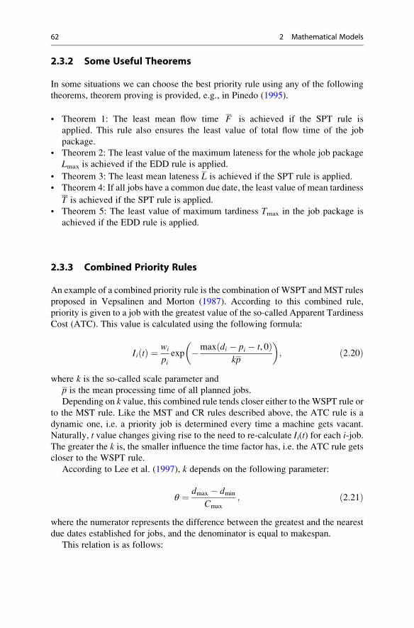
2.3.2 Some Useful Theorems
In some situations we can choose the best priority rule using any of the following
theorems, theorem proving is provided, e.g., in Pinedo (1995).
• Theorem 1: The least mean flow time F is achieved if the SPT rule is
applied. This rule also ensures the least value of total flow time of the job
package.
• Theorem 2: The least value of the maximum lateness for the whole job package
Lmax is achieved if the EDD rule is applied.
• Theorem 3: The least mean lateness L is achieved if the SPT rule is applied.
• Theorem 4: If all jobs have a common due date, the least value of mean tardiness
T is achieved if the SPT rule is applied.
• Theorem 5: The least value of maximum tardiness Tmax in the job package is
achieved if the EDD rule is applied.
2.3.3 Combined Priority Rules
An example of a combined priority rule is the combination of WSPT and MST rules
proposed in Vepsalinen and Morton (1987). According to this combined rule,
priority is given to a job with the greatest value of the so-called Apparent Tardiness
Cost (ATC). This value is calculated using the following formula:
Ii tð Þ ¼ wi
piexp �max di � pi � t, 0ð Þ
kp
� �; ð2:20Þ
where k is the so-called scale parameter and
p is the mean processing time of all planned jobs.
Depending on k value, this combined rule tends closer either to the WSPT rule or
to the MST rule. Like the MST and CR rules described above, the ATC rule is a
dynamic one, i.e. a priority job is determined every time a machine gets vacant.
Naturally, t value changes giving rise to the need to re-calculate Ii(t) for each i-job.The greater the k is, the smaller influence the time factor has, i.e. the ATC rule gets
closer to the WSPT rule.
According to Lee et al. (1997), k depends on the following parameter:
θ ¼ dmax � dmin
Cmax
; ð2:21Þ
where the numerator represents the difference between the greatest and the nearest
due dates established for jobs, and the denominator is equal to makespan.
This relation is as follows:
62 2 Mathematical Models
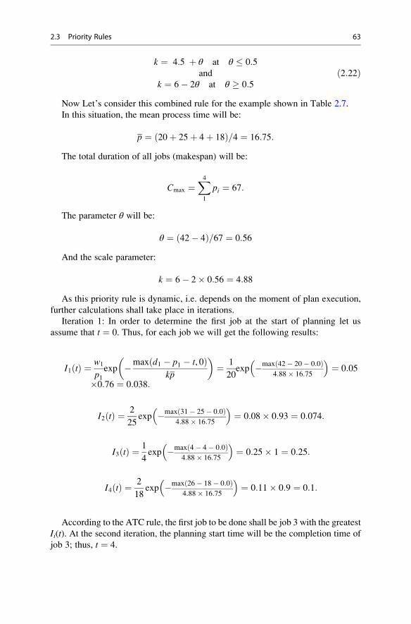
k ¼ 4:5 þ θ at θ � 0:5and
k ¼ 6� 2θ at θ � 0:5ð2:22Þ
Now Let’s consider this combined rule for the example shown in Table 2.7.
In this situation, the mean process time will be:
p ¼ 20þ 25þ 4þ 18ð Þ=4 ¼ 16:75:
The total duration of all jobs (makespan) will be:
Cmax ¼X41
pi ¼ 67:
The parameter θ will be:
θ ¼ ð42� 4Þ=67 ¼ 0:56
And the scale parameter:
k ¼ 6� 2� 0:56 ¼ 4:88
As this priority rule is dynamic, i.e. depends on the moment of plan execution,
further calculations shall take place in iterations.
Iteration 1: In order to determine the first job at the start of planning let us
assume that t ¼ 0. Thus, for each job we will get the following results:
I1 tð Þ ¼ w1
p1exp �max d1 � p1 � t, 0ð Þ
kp
� �¼ 1
20exp �max 42� 20� 0:0ð Þ
4:88� 16:75
� �¼ 0:05
�0:76 ¼ 0:038:
I2 tð Þ ¼ 2
25exp �max 31� 25� 0:0ð Þ
4:88� 16:75
� �¼ 0:08� 0:93 ¼ 0:074:
I3 tð Þ ¼ 1
4exp �max 4� 4� 0:0ð Þ
4:88� 16:75
� �¼ 0:25� 1 ¼ 0:25:
I4 tð Þ ¼ 2
18exp �max 26� 18� 0:0ð Þ
4:88� 16:75
� �¼ 0:11� 0:9 ¼ 0:1:
According to the ATC rule, the first job to be done shall be job 3 with the greatest
Ii(t). At the second iteration, the planning start time will be the completion time of
job 3; thus, t ¼ 4.
2.3 Priority Rules 63

Iteration 2: t ¼ 4.
I1 tð Þ ¼ 1
20exp �max 42� 20� 4:0ð Þ
4:88� 16:75
� �¼ 0:05� 0:8 ¼ 0:04:
I2 tð Þ ¼ 2
25exp �max 31� 25� 4:0ð Þ
4:88� 16:75
� �¼ 0:08� 0:97 ¼ 0:078:
I4 tð Þ ¼ 2
18exp �max 26� 18� 4:0ð Þ
4:88� 16:75
� �¼ 0:11� 0:95 ¼ 0:1:
According to Iteration 2, the second job to be done shall be job 4 that will end at
t ¼ 4þ 18 ¼ 22. Let us apply the same procedure to Iteration 3.
Iteration 3: t ¼ 22.
I1 tð Þ ¼ 1
20exp �max 42� 20� 22:0ð Þ
4:88� 16:75
� �¼ 0:05� 1 ¼ 0:05:
I2 tð Þ ¼ 2
25exp �max 31� 25� 22:0ð Þ
4:88� 16:75
� �¼ 0:08� 1 ¼ 0:08:
As we can see, the third job to be done shall be job 2. The resulting job sequence
will be {3, 4, 2, 1} and this coincides with the job sequence calculated above using
the EDD rule.
2.4 Production Intensity and Utility of Orders
The key purpose of the above priority rules is to consequently assign vacant
machines to items ready for processing exactly at such machines. Technically,
this concept is absolutely true as any planning engineer will take this into account
when planning a shift task. However, it is clear that the practical worthiness of such
algorithms will depend on the fact whether a correct criterion has been selected
to determine the sequence of processing of competing batches under given
circumstances.
Due to difficulties associated with the selection of criteria to determine the
processing sequence, instead of IT systems it is a user who has to decide and select
from a vast range of potential choices (up to 100). Such an approach does not seem
reasonable.
In addition to difficult selection of criteria to determine the sequence of compet-
ing batches, there is another problem that makes shift task planning even more
challenging. This is a substantial uncertainty about the batch readiness for
64 2 Mathematical Models
processing. In practice, when planning a shift task a planning engineer never has
complete information on the status of all manufactured batches. Besides, planning
takes place and the next shift starts at different time points; this makes uncertainty
about batch readiness for processing even more acute.
2.4.1 Production Intensity
When criteria for an optimal plan to be performed are determined, in addition to
process or economic factors, we also should take account of personal relations
between responsible persons. According to Afonichkin and Mikhailenko (2009),
there are two key courses of decision-making, i.e. rational and psychological. As for
the rational course, decisions are based on mathematically proven results, while
psychological course of decision-making is substantially based on intuition and
psychology of employees. A good production plan should be well balanced
between needs and wishes of all people involved in the production process.
People involved in the production process are all part of an extensive network of
relations that can be considered as a certain psychological field. Each field,
e.g. magnetic or electric, has a quantitative characteristic that is called “intensity”.
Similarly, a psychological field arising during production process can also be
described quantitatively; this quantitative description is called the production
intensity H (Mauergauz 1999). However, unlike physical fields, production inten-
sity cannot be measured physically; it has no physical dimensions, i.e. it is a
dimensionless value.
Such dimensionless intensity of a psychological field (whether large or small)
can only be estimated by comparison with another field or with another state of this
field, e.g., at any other point of time. We face a natural question how to calculate
production intensity.
For the purpose of intensity quantification, let us note that the situation in a
production shop is mainly characterized by two factors, i.e. total time required for
job completion and slack time. Please remember the so-called dynamic priority
rules described above that take account of these two factors. These rules include the
Minimum Slack Time (MST), Critical Ratio (CR), and the Apparent Tardiness Cost
(ATC) rules.
However, criteria that are calculated under any of these rules have substantial
deficiencies. First of all, there is no way to determine the values of such criteria if
the job due date has already expired by the start of planning. However, the most
important thing is that the cumulative machine and personnel load resulting from
different jobs cannot be determined using such criteria.
Unlike the above dynamic priority rules, we can determine production intensity
values not only for each job but for each machine and for the production shop on the
whole. Production intensity for a certain machine will be equal to the sum of
intensities for jobs awaiting processing on such machine, while production intensity
for a production shop on the whole equals to the sum of intensities for all jobs or,
which is the same, for all machines.
2.4 Production Intensity and Utility of Orders 65
The total time required to perform “handed down” plan targets is made of two
values, i.e. the production processing time and setup/job transfer time. Slack time
can be a positive or negative value or be equal to zero. Therefore, calculation
relations used to determine production intensity shall be different at different signs
of slack time values.
Thus, for one i-job:
Hi ¼ T1i þ T2ið Þ=z1i at di � t � 0
and
Hi ¼ T1i þ T2ið Þ � z2i at di � t � 0;ð2:23Þ
where T1i is the time duration determined by processing time pending at the time of
planning, T2i is the time component arising from the need to transfer jobs for further
processing, z1i is the production slack time in relation to plan targets, and z2i is thetardiness from plan targets.
T1i can be determined based on the following relation:
T1i ¼ 1
G
Xnij¼ki
pij 1� ηij=100�
mij; ð2:24Þ
where ki is the number of the first unfinished j-operation for i-job, ni is the total
number of operations required to perform i-job, pij is the processing time of
each remaining operation in hours or days, ηij is the coefficient of readiness of
j-operation (%), mij is the number of simultaneously processed items of i-job duringj-operation, andG is the average number of work hours or days in a planning period.
ηij can be other than zero only if j ¼ ki, i.e. when the first unfinished operation isin process. This coefficient is used to take account of intensity of a job that is in
process. If a planned job is to produce a batch of items or assembly parts, a certain
operation allows simultaneous processing of multiple items or parts, e.g., on
parallel machines. If each machine processes one item only, mij will be equal to
the number of machines involved in parallel processing of one planned job. G, thedenominator, is used in formula (2.24) to ensure that H1i is dimensionless.
T2i is calculated using the following relation:
T2i ¼ 1
G
Xnij¼ki
sij; ð2:25Þ
where sij is the duration of required transportation and machine setup associated
with j-operation for i-job.Let us assume the following relation for dimensionless slack time available to a
planning engineer:
z1i ¼ di � t
αGþ 1; ð2:26Þ
66 2 Mathematical Models
where α is the “psychological” coefficient of a given enterprise representing the
level of “complacency” at available slack times or the level of “nervousness” if
production due dates are failed to meet.
And, finally:
z2i ¼ t� diαG
þ 1: ð2:27Þ
Similarly to the WSPT or ATC rules described above, intensity of a certain job
can include a respective weight coefficient of priority wi. In particular, in the
simplest case (where all readiness coefficients ηij ¼ 0, the number of simulta-
neously processed items under one job mij ¼ 1, planning takes place for the first
operation and all ki ¼ 1, while transportation and setup time sij can be ignored)
intensity can be determined using the following formulas:
Hi ¼ wipiG
1
di � tð Þ=αGþ 1at di � t � 0
and
Hi ¼ wipiG
t� dið Þ=αGþ 1ð Þ at di � t � 0:
ð2:28Þ
Now let us consider the relation between intensity and available slack time or
deadline tardiness (Fig. 2.6).
The slack time (difference between the due date for each job di and the current
time point t) is plotted on the X-line. On the positive part, i.e. wheredi > t, intensityvalues decrease hyperbolically as far as slack time increases. If slack time is
negative, i.e. there are tardiness on plan targets di < t, intensity values increase
linearly as far as tardiness increases. In expressions (2.26) and (2.27) ifdi ¼ t, i.e. atthe point of transfer from one relation to another, z1 ¼ z2 ¼ 1. Intensity values
calculated using formulas (2.23) or (2.28) also coincide at this point. Besides, this
point also sees the match of values for the following derivative:
H
d2 - t
H2H1
Job 2
Job 1
0
p2
p1
H p1< p2
di - tdi - t0
1
α
α α
2
1 < 2
a) b)
α α
Fig. 2.6 Relation between production intensity and slack time (a) at different psychological
coefficient α; (b) at different job processing time pi
2.4 Production Intensity and Utility of Orders 67
dH
d di � tð Þ ;
which have been calculated been using both formulas. Thus, the straight line in the
left-hand part of the chart is tangent at the transition point to the hyperbolic curve in
the right-hand part of the chart.
Figure 2.6a shows two curves for H changes; these curves differ by the value of
“psychological” coefficient α; note that α2 > α1. As we can see, the greater the α is,
the less intensity is associated with tardiness; however, the level of “relaxation” is
also lower when slack time is available. Therefore, we can consider α as a factor of
balance for relations at production.
Figure 2.6b shows two charts of intensity dependency on di � t at different pivalues. The charts display the position of two jobs with different values of pi anddi � t. In this case, as di ¼ t for job 1, then, assuming that w1 ¼ 1, Eq. (2.28) yields
that H1 ¼ p1G. As di � t � 0 for job 2, intensity will be:
H2 ¼ p2G
1
d2 � tð Þ=αGþ 1:
As we can see from Fig. 2.6b, even if di � t ¼ 0 (as true for job 1), it is still
possible that the intensity associated with another job where di > t will be greater,i.e. H2 > H1, and job 2 will have priority over job 1. This feature makes the
intensity-based priority rule substantially different from, for example, the Critical
Ratio Rule.
Let us consider how to use the intensity parameter to determine the sequence of
jobs shown in Table 2.8. As intensity is a dynamic criterion as its value depends on
time t, calculations will include multiple iterations similar to the procedure applied
under the CR, ATC, and other rules. The planning period G is assumed 30 days and
the “psychological” coefficient α ¼ 0:1.Iteration 1: To determine the first job to be done, at the start of planning it is
assumed that t ¼ 0. As for all jobs in Table 2.7 di > t, we use the first formula from
(2.28).
H1 ¼ w1p1G
1
d1 � tð Þ=αGþ 1¼ 1� 20
30
1
42� 0ð Þ=0:1=30þ 1¼ 0:66� 0:07 ¼ 0:044:
Table 2.8 Planning inputs
Items
Capacity, items per day
Cost per item Minimum daily outputType 1 Type 2
A1 20 15 6 1510
A2 35 30 4 4500
68 2 Mathematical Models
H2 ¼ 2� 25
30
1
31� 0ð Þ=0:1=30þ 1¼ 1:66� 0:09 ¼ 0:14:
H3 ¼ 1� 4
30
1
4� 0ð Þ=0:1=30þ 1¼ 0:13� 0:42 ¼ 0:06:
H4 ¼ 2� 18
30
1
26� 0ð Þ=0:1=30þ 1¼ 1:2� 0:1 ¼ 0:12:
The first job to be done shall be the job with the greatest intensity, i.e. job 2. This
job will be released at t ¼ 25. At this point di > t is still true for jobs 1 and 4;
however, di < t for job 3. Accordingly, we still use the first formula from (2.28) to
determine intensity for jobs 1 and 4, while job 3 intensity should be calculated
based on the second formula from (2.28).
Iteration 2: t ¼ 25.
H1 ¼ 1� 20
30
1
42� 25ð Þ=0:1=30þ 1¼ 0:66� 0:15 ¼ 0:1:
H3 ¼ w3p3G
t� d3ð Þ=αGþ 1ð Þ ¼ 1� 4
3025� 4ð Þ=0:1=30þ 1ð Þ ¼ 0:13� 8
¼ 1:06:
H4 ¼ 2� 18
30
1
26� 25ð Þ=0:1=30þ 1¼ 1:2� 0:75 ¼ 0:9:
Thereafter, job 3 will have the greatest intensity. Job 3 will be start at
t ¼ 25þ 4 ¼ 29. By this time, job 4 will become past due, and we should use the
second formula from (2.28) to determine its intensity.
Iteration 3: t ¼ 29.
H1 ¼ 1� 20
30
1
42� 29ð Þ=0:1=30þ 1¼ 0:66� 0:18 ¼ 0:12:
H4 ¼ 2� 18
3029� 26ð Þ=0:1=30þ 1ð Þ ¼ 1:2� 2 ¼ 2:4:
2.4 Production Intensity and Utility of Orders 69
Thereafter, job 4 will have the greatest intensity. The resulting job sequence will
be {2, 3, 4, 1}. Now let us calculate the objective function Tw using the same
procedure as for other rules described above.
Job sequence 0 (2/25) 25 (3/4) 29 (4/18) 47 (1/20) 67
Due date (2) 31 (3) 4 (4) 26 (1) 42
Tardiness �6 25 21 25
Objective function value Tw ¼ 2� 0þ 1� 25þ 2� 21þ 1� 25 ¼ 92
2.4.2 Dynamic Utility Function of Orders
As we can see from the previous example, the intensity-based priority rule yields
substantially worse values of the objective function Tw as compared with, for
example, the EDD or SPT rules (refer to Sect. 3.2.1). This is inevitable as according
to Theorem 5 (Sect. 2.3.2) the least tardiness results from the EDD rule. However,
intensity-based priority rule gives much better results if we use other criteria as the
objective function, for example, the weighted sum of tardiness costs fw (2.19). The
procedure of applying the intensity-based rule will be further described for such
a case.
As the production intensity has the additive property, when we use intensity to
describe statuses of jobs during planning, we can get a wide range of evaluations for
the production situation, i.e. we can compare intensities for different machines,
production shops and floors, orders, etc. In this paragraph, we will describe how to
use the production intensity to determine dynamic utility of orders.
Basically, we can use functions of the dynamic utility of orders V to evaluate
whether it is possible and desirable to ensure a high level of customer service C1
(Table 2.3). In order to identify evaluation rules, let us consider how to apply
typical utility functions described in Sect. 1.7.2.
Let us assume that any order is quite useful for a manufacturer in a certain
prospect. Note that the greater the order scope and order fulfilment time is, the
greater utility such order will have. In such a way, the possibility of order fulfilment
in future certainly has a positive utility and should yield a respective gain.
On the other hand, the closer the due date for an order is, a manufacturer starts
facing certain difficulties. The utility value starts decreasing. However, if the
manufacturer manages to perform the order when due, the order utility remains
positive till the very time of order execution, and utility becomes zero at the time of
completion. If the manufacturer fails to meet the due date, he usually gets into
troubles with this. The order becomes the source of losses, thus having a negative
utility.
As we can see, if slack time is available for an order, a manufacturer generally
counts on gain while in case of tardiness it incurs losses. The behavior of utility as a
potential gain/loss function is described in numerous sources. Generally, all
research results can be reduced to two options shown in Fig. 2.7.
70 2 Mathematical Models
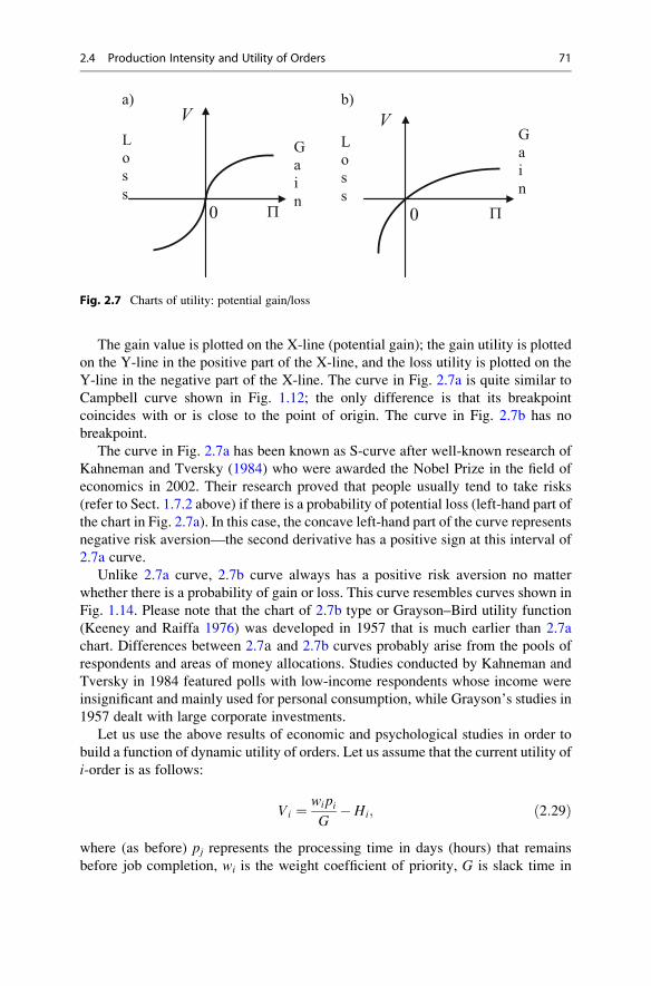
The gain value is plotted on the X-line (potential gain); the gain utility is plotted
on the Y-line in the positive part of the X-line, and the loss utility is plotted on the
Y-line in the negative part of the X-line. The curve in Fig. 2.7a is quite similar to
Campbell curve shown in Fig. 1.12; the only difference is that its breakpoint
coincides with or is close to the point of origin. The curve in Fig. 2.7b has no
breakpoint.
The curve in Fig. 2.7a has been known as S-curve after well-known research of
Kahneman and Tversky (1984) who were awarded the Nobel Prize in the field of
economics in 2002. Their research proved that people usually tend to take risks
(refer to Sect. 1.7.2 above) if there is a probability of potential loss (left-hand part of
the chart in Fig. 2.7a). In this case, the concave left-hand part of the curve represents
negative risk aversion—the second derivative has a positive sign at this interval of
2.7a curve.
Unlike 2.7a curve, 2.7b curve always has a positive risk aversion no matter
whether there is a probability of gain or loss. This curve resembles curves shown in
Fig. 1.14. Please note that the chart of 2.7b type or Grayson–Bird utility function
(Keeney and Raiffa 1976) was developed in 1957 that is much earlier than 2.7a
chart. Differences between 2.7а and 2.7b curves probably arise from the pools of
respondents and areas of money allocations. Studies conducted by Kahneman and
Tversky in 1984 featured polls with low-income respondents whose income were
insignificant and mainly used for personal consumption, while Grayson’s studies in
1957 dealt with large corporate investments.
Let us use the above results of economic and psychological studies in order to
build a function of dynamic utility of orders. Let us assume that the current utility of
i-order is as follows:
Vi ¼ wipiG
� Hi; ð2:29Þ
where (as before) pj represents the processing time in days (hours) that remains
before job completion, wi is the weight coefficient of priority, G is slack time in
P P0 0
VV
Gai
n
Gai
n
b)a)
Los
s
Los
s
Fig. 2.7 Charts of utility: potential gain/loss
2.4 Production Intensity and Utility of Orders 71
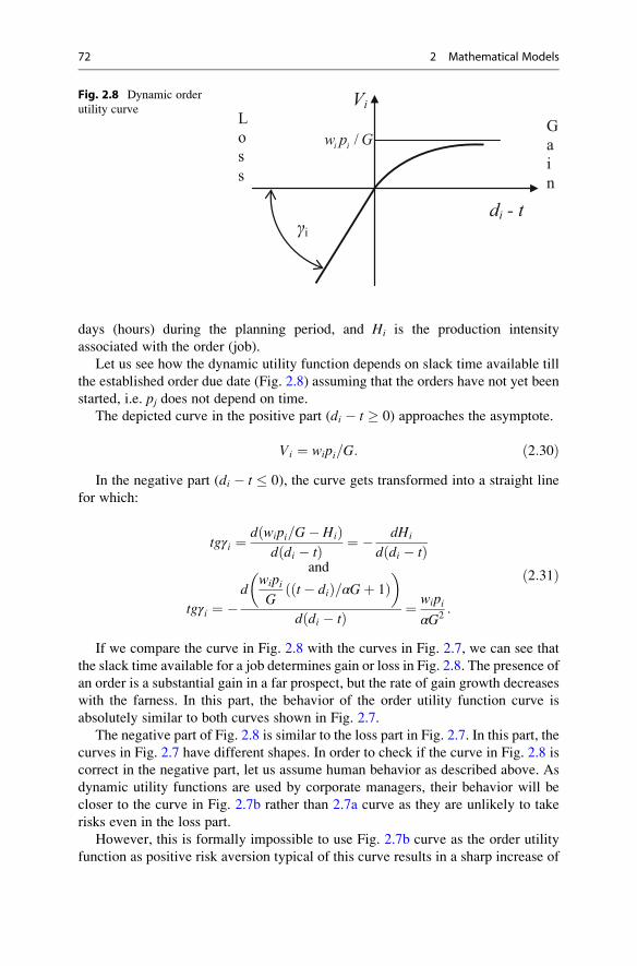
days (hours) during the planning period, and Hi is the production intensity
associated with the order (job).
Let us see how the dynamic utility function depends on slack time available till
the established order due date (Fig. 2.8) assuming that the orders have not yet been
started, i.e. pj does not depend on time.
The depicted curve in the positive part (di � t � 0) approaches the asymptote.
Vi ¼ wipi=G: ð2:30ÞIn the negative part (di � t � 0), the curve gets transformed into a straight line
for which:
tgγi ¼d wipi=G� Hið Þ
d di � tð Þ ¼ � dHi
d di � tð Þand
tgγi ¼ �d
wipiG
t� dið Þ=αGþ 1ð Þ� �
d di � tð Þ ¼ wipiαG2
:
ð2:31Þ
If we compare the curve in Fig. 2.8 with the curves in Fig. 2.7, we can see that
the slack time available for a job determines gain or loss in Fig. 2.8. The presence of
an order is a substantial gain in a far prospect, but the rate of gain growth decreases
with the farness. In this part, the behavior of the order utility function curve is
absolutely similar to both curves shown in Fig. 2.7.
The negative part of Fig. 2.8 is similar to the loss part in Fig. 2.7. In this part, the
curves in Fig. 2.7 have different shapes. In order to check if the curve in Fig. 2.8 is
correct in the negative part, let us assume human behavior as described above. As
dynamic utility functions are used by corporate managers, their behavior will be
closer to the curve in Fig. 2.7b rather than 2.7a curve as they are unlikely to take
risks even in the loss part.
However, this is formally impossible to use Fig. 2.7b curve as the order utility
function as positive risk aversion typical of this curve results in a sharp increase of
γi
/i iw p G
Vi
di - t
Gai
n
Los
s
Fig. 2.8 Dynamic order
utility curve
72 2 Mathematical Models
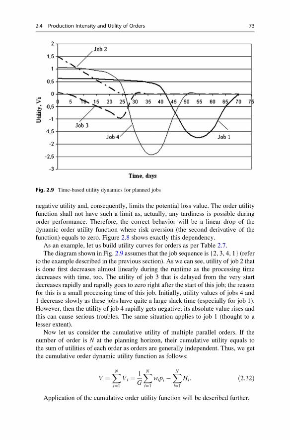
negative utility and, consequently, limits the potential loss value. The order utility
function shall not have such a limit as, actually, any tardiness is possible during
order performance. Therefore, the correct behavior will be a linear drop of the
dynamic order utility function where risk aversion (the second derivative of the
function) equals to zero. Figure 2.8 shows exactly this dependency.
As an example, let us build utility curves for orders as per Table 2.7.
The diagram shown in Fig. 2.9 assumes that the job sequence is {2, 3, 4, 1} (refer
to the example described in the previous section). As we can see, utility of job 2 that
is done first decreases almost linearly during the runtime as the processing time
decreases with time, too. The utility of job 3 that is delayed from the very start
decreases rapidly and rapidly goes to zero right after the start of this job; the reason
for this is a small processing time of this job. Initially, utility values of jobs 4 and
1 decrease slowly as these jobs have quite a large slack time (especially for job 1).
However, then the utility of job 4 rapidly gets negative; its absolute value rises and
this can cause serious troubles. The same situation applies to job 1 (thought to a
lesser extent).
Now let us consider the cumulative utility of multiple parallel orders. If the
number of order is N at the planning horizon, their cumulative utility equals to
the sum of utilities of each order as orders are generally independent. Thus, we get
the cumulative order dynamic utility function as follows:
V ¼XNi¼1
Vi ¼ 1
G
XNi¼1
wipi �XNi¼1
Hi: ð2:32Þ
Application of the cumulative order utility function will be described further.
Fig. 2.9 Time-based utility dynamics for planned jobs
2.4 Production Intensity and Utility of Orders 73

2.5 More Complex Models of Linear Optimization
The problem described above in Sect. 2.1.2 deals with the linear optimization
model that allows continuous changes of variables. However, this is not true in
many situations where variables can take certain values only, for instance, integers.
2.5.1 Integer Linear Optimization Model
Let us take the following example to consider such model. We assume that a
production shop has 100 machines of type 1 and 200 machines of type 2; machines
of each type can produce items A1 and A2. Table 2.8 shows machine capacities, the
cost of item for each type, and minimum daily output plan.
The planning task is to calculate the number xij of machines of j-type, j ¼ 1, 2,
which should be allocated to manufacture items Ai, i ¼ 1, 2 provided that the
maximum price f(x) of output products manufactured per day is achieved.
In this situation, the objective function (the daily output price) shall tend to the
maximum value, i.e.
f xð Þ ¼ 20� 6� x11 þ 15� 6� x12 þ 35� 4� x21 þ 30� 4� x22! max: ð2:33Þ
The limits on machine count are as follows:
x11 þ x21 ¼ 100
and
x12 þ x22 ¼ 200:ð2:34Þ
Minimum output limits are as follows:
20� x11 þ 15� x12 � 1510
and
35� x21 þ 30� x22 � 4500:ð2:35Þ
Besides, we need to specify that xij can take positive values only
xij > 0 ð2:36Þand must be integers.
Figure 2.10 shows how this task is solved using MS Excel. The solution is very
much alike to the solution obtained in Sect. 2.1.2 (Fig. 2.3). The difference is that
we need to apply the constraint that each variable shall be non-negative. The
constraints that variables must be integers are entered directly into MS Excel in
74 2 Mathematical Models
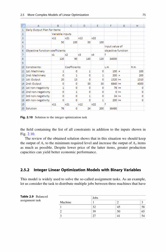
the field containing the list of all constraints in addition to the inputs shown in
Fig. 2.10.
The review of the obtained solution shows that in this situation we should keep
the output of A1 to the minimum required level and increase the output of A2 items
as much as possible. Despite lower price of the latter items, greater production
capacities can yield better economic performance.
2.5.2 Integer Linear Optimization Models with Binary Variables
This model is widely used to solve the so-called assignment tasks. As an example,
let us consider the task to distribute multiple jobs between three machines that have
Fig. 2.10 Solution to the integer optimization task
Table 2.9 Balanced
assignment taskMachine
Jobs
1 2 3
1 32 45 58
2 39 50 65
3 27 41 54
2.5 More Complex Models of Linear Optimization 75
similar process functions but different capacities. If the number of jobs to be
assigned equals to the number of machines, the task is called balanced; otherwise,
the task is non-balanced.
First, let us consider the case where there are three jobs, i.e. the task is balanced.
Table 2.9 shows runtime values for each job (in hours).
We assume that all machines have the same cost of 1 h of operation. Then, it
seems practical to distribute jobs between machines in such a way that ensures the
minimum total operating time of all machines. In order to solve assignment tasks,
we need to introduce the so-called binary variables that may take one of the
following possible values only, i.e. 0 or 1. Let us denote such variables as δij todescribe if it is possible to assign i-job to j-machine. If such assignment is possible,
then δij ¼ 1; otherwise, δij ¼ 0.
The presence of binary variables in a model automatically limits possible values
of such variables. If a job is assigned to a certain machine, such job cannot be
assigned to another machine and, accordingly, a busy machine cannot be used for
another job.
The objective function will be as follows:
f δð Þ ¼ 32� δ11 þ 45� δ21 þ 58� δ31 þ 39� δ12 þ 50� δ22þ65� δ32 þ 27� δ13 þ 41� δ23 þ 54� δ33
! min: ð2:37Þ
Machine load limits will be:
δ11 þ δ21 þ δ11 ¼ 1;δ12 þ δ22 þ δ32 ¼ 1;δ13 þ δ23 þ δ33 ¼ 1:
ð2:38Þ
Job assignment limits will be:
δ11 þ δ12 þ δ13 ¼ 1;δ21 þ δ22 þ δ23 ¼ 1;δ31 þ δ32 þ δ33 ¼ 1:
ð2:39Þ
And we also need to add constraints of variable’s binary.
Figure 2.11 shows the task solution using MS Excel. As we can see, job 3 is
assigned to machine 1, job 2 is assigned to machine 2, and job 1 is assigned to
machine 3. Actually, this plan seems quite surprising. On the face of it, it appears
that the most productive machine 3 should have assigned the most prolonged job
3 and machine 2 with low capacity should do the least prolonged job 1. However,
detailed calculations disprove this intuitive assumption.
For your reference, Fig. 2.12 shows the objective function settings and task
constraints in MS Excel.
Now, let us add another job to this task to make more complex (refer to
Fig. 2.13). The task is non-balanced now and we have to assign two jobs to one
machine. In this situation, the objective function (2.37) will have 12 δij variables
76 2 Mathematical Models
instead of 9. The number of constraints (2.38) will remain the same (3) according to
the number of jobs; however, the left-hand part will have 4 δij variables and it can beequal or more than 1. Constraints (2.39) will remain the same, but their number will
increase to 4 (one constraint per each job).
Fig. 2.11 Job distribution between three parallel machines
Fig. 2.12 Constraints screen
2.5 More Complex Models of Linear Optimization 77
The task solution displayed in the lower part of Fig. 2.13 shows that two jobs are
assigned to the most productive machine 3 (as expected) and remaining machines
have one job each.
2.6 Fixed Job Sequence Models
At the beginning of this chapter we named three main planning challenges,
i.e. What products? What quantity? When? Task and solving methods described
above do not deal with the practical and reasonable choice of product types. The
above tasks mainly deal with the optimal quantity of products to be manufactured
or delivered based on a certain criterion. The job sequence can be determined
under different rules. This causes a wide spread of values of the objective function.
Besides, any of the applied rules does not warranty an accurate and explicit solution
to the optimization task (except for a number of special cases described in
Sect. 2.3.2). In this section, we will describe the so-called branch-and-bound
method that allows obtaining accurate and explicit solutions.
As a general matter, there is no universal algorithm that yields an optimal solution.
Therefore, various planning situations require different versions of the branch-and-
bound method that are the most appropriate under given circumstances.
Fig. 2.13 Distribution of four jobs between three machines
78 2 Mathematical Models
2.6.1 Branch-and-Bound Method with Minimum CumulativeTardiness Tw
The branch-and-bound method includes two procedures: branching and bounding
(finding value limits). Branching is to split the feasible region (set of candidate
solutions) into smaller subsets. Its recursive application results in a search tree orthe branch-and-bound tree. The nodes of this tree represent subsets of candidate
solutions. Bounding is to compute upper and/or lower bounds to find an optimal
solution within feasible subsets.
Branching and bounding procedures can be different for different tasks. First
of all, branching and bounding can start either at the final or initial stage of
job performance. In the first case, it is better to use the algorithm described in
(Sule 2007).
Let us see how to apply the branch-and-bound method using the example as per
Table 2.7. As the objective function of planning, the same as in Sect. 2.3.1 we take
minimized Tw that is the cumulative weighted tardiness (2.18). As the required
sequence includes 4 jobs, the search tree will also have 4 levels.
In order to build the search tree let us remember that any of the four jobs as per
Table 2.7 can, in fact, go to the last in the job sequence. Now let us determine which
of the jobs will have the least effect on Tw if performed last, i.e. we will find the
lower bound of Tw. The best way to graphically display step operations to find a
solution is to build a search tree (refer to Fig. 2.14).
Level 4 contains 4 nodes that reflect all possible jobs as per Table 2.7. In order to
determine Tw for each node at this level, let us calculate the total processing time of
all jobs:
Node 1Job 1
wT ³ 25
Node 2Job 2
wT ³ 72
Node 3Job 3
wT ³ 63
Node 4Job 4
wT ³ 82
Level 4
Node 5Job 2
wT ³ 57
Node 6Job 3
wT ³ 68
Node 7Job 4
wT ³ 67
Level 3
Node 8Job 3
wT ³ 75
Node 9Job 4
wT ³ 57
Level 2
Node 10Job 3
wT = 57
Level 1
Fig. 2.14 Search tree for cumulative tardiness Tw
2.6 Fixed Job Sequence Models 79
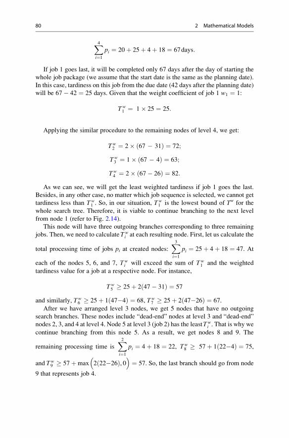
X4i¼1
pi ¼ 20þ 25þ 4þ 18 ¼ 67days:
If job 1 goes last, it will be completed only 67 days after the day of starting the
whole job package (we assume that the start date is the same as the planning date).
In this case, tardiness on this job from the due date (42 days after the planning date)
will be 67� 42 ¼ 25 days. Given that the weight coefficient of job 1 w1 ¼ 1:
Tw1 ¼ 1� 25 ¼ 25:
Applying the similar procedure to the remaining nodes of level 4, we get:
T w2 ¼ 2� ð67 � 31Þ ¼ 72;
T w3 ¼ 1� ð67 � 4Þ ¼ 63;
Tw4 ¼ 2� ð67� 26Þ ¼ 82:
As we can see, we will get the least weighted tardiness if job 1 goes the last.
Besides, in any other case, no matter which job sequence is selected, we cannot get
tardiness less than T w1 . So, in our situation, T w
1 is the lowest bound of Tw for the
whole search tree. Therefore, it is viable to continue branching to the next level
from node 1 (refer to Fig. 2.14).
This node will have three outgoing branches corresponding to three remaining
jobs. Then, we need to calculate T wi at each resulting node. First, let us calculate the
total processing time of jobs pi at created nodes:X3i¼1
pi ¼ 25þ 4þ 18 ¼ 47. At
each of the nodes 5, 6, and 7, Twi will exceed the sum of T w
1 and the weighted
tardiness value for a job at a respective node. For instance,
T w5 � 25þ 2ð47� 31Þ ¼ 57
and similarly, T w6 � 25þ 1ð47�4Þ ¼ 68, Tw
7 � 25þ 2ð47�26Þ ¼ 67.
After we have arranged level 3 nodes, we get 5 nodes that have no outgoing
search branches. These nodes include “dead-end” nodes at level 3 and “dead-end”
nodes 2, 3, and 4 at level 4. Node 5 at level 3 (job 2) has the leastT wi . That is why we
continue branching from this node 5. As a result, we get nodes 8 and 9. The
remaining processing time isX2i¼1
pi ¼ 4þ 18 ¼ 22, Tw8 � 57þ 1ð22�4Þ ¼ 75,
and T w9 � 57þmax
�2ð22�26Þ, 0
�¼ 57. So, the last branch should go from node
9 that represents job 4.
80 2 Mathematical Models
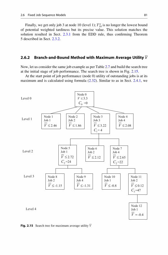
Finally, we get only job 3 at node 10 (level 1); T w10 is no longer the lowest bound
of potential weighted tardiness but its precise value. This solution matches the
solution resulted in Sect. 2.3.1 from the EDD rule, thus confirming Theorem
5 described in Sect. 2.3.2.
2.6.2 Branch-and-Bound Method with Maximum Average Utility V
Now, let us consider the same job example as per Table 2.7 and build the search tree
at the initial stage of job performance. The search tree is shown in Fig. 2.15.
At the start point of job performance (node 0) utility of outstanding jobs is at its
maximum and is calculated using formula (2.32). Similar to as in Sect. 2.4.1, we
Node 2Job 2
V £ 1.86
Node 3Job 3
V £ 3.22
1C = 4
Node 1Job 1
V £ 2.46
Node 4Job 4
V £ 2.08
Node 5Job 1
V £ 2.72
2C =24
Node 6Job 2
V £ 2.12
Node 7Job 4
V £ 2.65
2C =22
Node 0
V £ 3.3
0C =0
Level 1
Level 0
Level 2
Node 9Job 4
V £ -1.31
Node 8Job 2
V £ -1.15
Level 3
Node 12Job 1
V = -0.4
Level 4
Node 11Job 2
V £ 0.12
3C =47
Node 10Job 1
V £ -0.8
Fig. 2.15 Search tree for maximum average utility V
2.6 Fixed Job Sequence Models 81
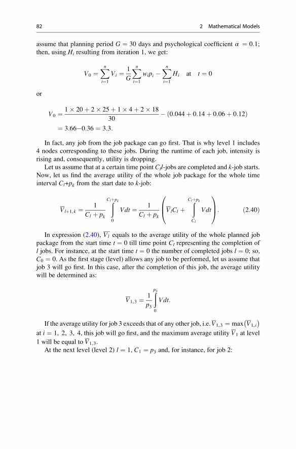
assume that planning period G ¼ 30 days and psychological coefficient α ¼ 0:1;then, using Hi resulting from iteration 1, we get:
V0 ¼Xni¼1
Vi ¼ 1
G
Xni¼1
wipi �Xni¼1
Hi at t ¼ 0
or
V0 ¼ 1� 20þ 2� 25þ 1� 4þ 2� 18
30� ð0:044þ 0:14þ 0:06þ 0:12Þ
¼ 3:66�0:36 ¼ 3:3:
In fact, any job from the job package can go first. That is why level 1 includes
4 nodes corresponding to these jobs. During the runtime of each job, intensity is
rising and, consequently, utility is dropping.
Let us assume that at a certain time point Cll-jobs are completed and k-job starts.Now, let us find the average utility of the whole job package for the whole time
interval Cl+pk from the start date to k-job:
Vlþ1,k ¼ 1
Cl þ pk
ðClþpk
0
Vdt ¼ 1
Cl þ pkVlCl þ
ðClþpk
Cl
Vdt
0B@1CA: ð2:40Þ
In expression (2.40), Vl equals to the average utility of the whole planned job
package from the start time t ¼ 0 till time point Сl representing the completion of
l jobs. For instance, at the start time t ¼ 0 the number of completed jobs l ¼ 0; so,
C0 ¼ 0. As the first stage (level) allows any job to be performed, let us assume that
job 3 will go first. In this case, after the completion of this job, the average utility
will be determined as:
V1,3 ¼ 1
p3
ðp30
Vdt:
If the average utility for job 3 exceeds that of any other job, i.e.V1,3 ¼ max V1, i
� at i ¼ 1, 2, 3, 4, this job will go first, and the maximum average utility V1 at level
1 will be equal to V1,3.
At the next level (level 2) l ¼ 1, C1 ¼ p3 and, for instance, for job 2:
82 2 Mathematical Models
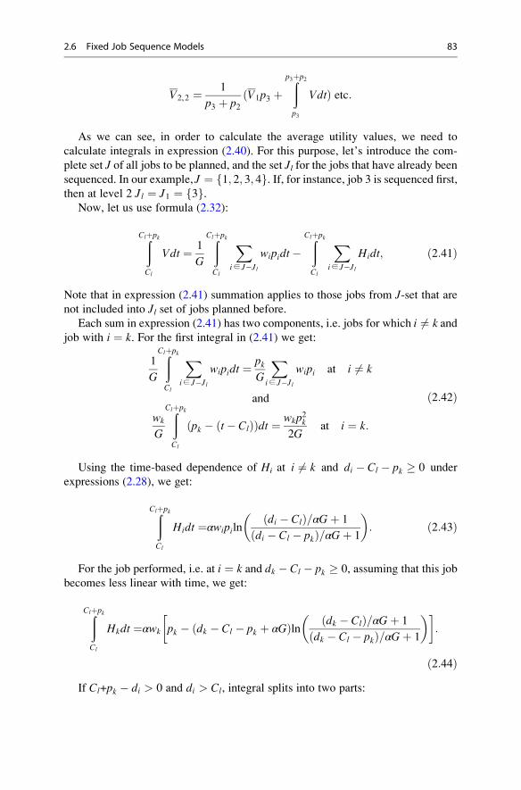
V2,2 ¼ 1
p3 þ p2ðV1p3 þ
ðp3þp2
p3
VdtÞ etc:
As we can see, in order to calculate the average utility values, we need to
calculate integrals in expression (2.40). For this purpose, let’s introduce the com-
plete set J of all jobs to be planned, and the set Jl for the jobs that have already beensequenced. In our example, J ¼ 1; 2; 3; 4f g. If, for instance, job 3 is sequenced first,then at level 2 Jl ¼ J1 ¼ 3f g.
Now, let us use formula (2.32):
ðClþpk
Cl
Vdt ¼ 1
G
ðClþpk
Cl
Xi∈ J�Jl
wipidt�ðClþpk
Cl
Xi∈ J�Jl
Hidt; ð2:41Þ
Note that in expression (2.41) summation applies to those jobs from J-set that arenot included into Jl set of jobs planned before.
Each sum in expression (2.41) has two components, i.e. jobs for which i 6¼ k andjob with i ¼ k. For the first integral in (2.41) we get:
1
G
ðClþpk
Cl
Xi∈ J�Jl
wipidt ¼pkG
Xi∈ J�Jl
wipi at i 6¼ k
and
wk
G
ðClþpk
Cl
pk � t� Clð Þð Þdt ¼ wkp2k
2Gat i ¼ k:
ð2:42Þ
Using the time-based dependence of Hi at i 6¼ k and di � Cl � pk � 0 under
expressions (2.28), we get:
ðClþpk
Cl
Hidt ¼αwipilndi � Clð Þ=αGþ 1
di � Cl � pkð Þ=αGþ 1
� �: ð2:43Þ
For the job performed, i.e. at i ¼ k and dk � Cl � pk � 0, assuming that this job
becomes less linear with time, we get:
ðClþpk
Cl
Hkdt ¼αwk pk � dk � Cl � pk þ αGð Þln dk � Clð Þ=αGþ 1
dk � Cl � pkð Þ=αGþ 1
� � �:
ð2:44ÞIf Cl+pk � di > 0 and di > Cl, integral splits into two parts:
2.6 Fixed Job Sequence Models 83

ðClþpk
Cl
Hidt ¼ðdiCl
HidtþðClþpk
di
Hidt: ð2:45Þ
At i 6¼ k the first part will be:
ðdiCl
Hidt ¼ αwipilndi � Cl
αGþ 1
� �And the second part will be :ðClþpk
di
Hidt ¼ αwipi2
Cl þ pk � diαG
þ 1
� �2
� 1
" #:
ð2:46Þ
For the job performed i ¼ k at Cl þ pk � dk > 0 and dk > Cl we get:
ðdkCl
Hkdt ¼ αwk dk � Cl þ ðCl þ pk � dk � αGÞln dk � Cl
αGþ 1
� � �andðClþpk
dk
Hkdt ¼ αwkðCl þ pkÞ2
Cl þ pk � dkαG
þ 1
� �2
� 1
" #
�wk
2G1� dk
αG
� �½ðCl þ pkÞ2 � d2k ��
wk
3αG2½ðCl þ pkÞ3 � d3k �:
ð2:47Þ
If Cl+pk � di > 0 and di � Cl, first two components in (2.46) and (2.47) will
become zero.
As an example, let us determine the average utilityV1,3 for job 3 at level 1. Here,
l ¼ 0, the set of jobs to be planned is empty Jl ¼ J0 and the start time of a new job
Cl ¼ C0 ¼ 0. So:
V1,3 ¼ 1
p3
ðp30
Vdt ¼ 1
G
Xi∈ J, i 6¼3
wipi þw3p32G
� 1
p3
Xi∈ J, i 6¼3
ðp30
Hidt� 1
p3
ðp30
H3dt: ð2:48Þ
The first and the second components in (2.48)
84 2 Mathematical Models
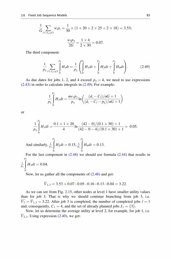
1
G
Xi∈ J, i6¼3
wipi ¼1
30� 1� 20þ 2� 25þ 2� 18ð Þ ¼ 3:53;
w3p32G
¼ 1� 4
2� 30¼ 0:07:
The third component:
1
p3
Xi∈ J, i 6¼3
ðp30
Hidt ¼ 1
p3
ðp30
H1dtþðp30
H2dtþðp30
H4dt
0@ 1A: ð2:49Þ
As due dates for jobs 1, 2, and 4 exceed p3 ¼ 4, we need to use expressions
(2.43) in order to calculate integrals in (2.49). For example:
1
p3
ðp30
H1dt ¼ αw1p1p3
lndi � Clð Þ=αGþ 1
di � Cl � pkð Þ=αGþ 1
� �
or
1
p3
ðp30
H1dt ¼ 0:1� 1� 20
4ln
42� 0ð Þ= 0:1� 30ð Þ þ 1
42� 0� 4ð Þ= 0:1� 30ð Þ þ 1¼ 0:05:
And similarly, 1p3
ðp30
H2dt ¼ 0:15, 1p3
ðp30
H4dt ¼ 0:13.
For the last component in (2.48) we should use formula (2.44) that results in
1p3
ðp30
H3dt ¼ 0:04.
Now, let us gather all the components of (2.48) and get:
V1,3 ¼ 3:53þ 0:07�0:05�0:16�0:13�0:04 ¼ 3:22:
As we can see from Fig. 2.15, other nodes at level 1 have smaller utility values
than for job 3. That is why we should continue branching from job 3, i.e.
V1 ¼ V1,3 ¼ 3:22. After job 3 is completed, the number of completed jobs l ¼ 1
and, consequently, C1 ¼ 4, and the set of already planned jobs J1 ¼ 3f g.Now, let us determine the average utility at level 2, for example, for job 1, i.e.
V2,1. Using expression (2.40), we get:
2.6 Fixed Job Sequence Models 85
V2,1 ¼ 1
C1 þ p1V1C1 þ
ðC1þp1
C1
Vdt
0B@1CA ¼ V1C1
C1 þ p1
þ p1C1 þ p1ð ÞG
Xi∈ J�J1, i 6¼1
wipi þw1p
21
2 C1 þ p1ð ÞG� 1
C1 þ p1
ðC1þp1
C1
Xi∈ J�J1
Hidt:
ð2:50Þ
The integral in (2.50) has three components corresponding to jobs 1, 2, and
4 with job 1 being performed; so, C1+p1 ¼ 4+20 ¼ 24. As the due dates for jobs
2 and 4 (Table 2.8) exceed C1+p1 ¼ 24, we should use expressions (2.43) to
calculate integrals in (2.50). The due date of job 1 also exceeds C1+p1 ; so, weshould calculate the respective integral in (2.50) using formula (2.44). Our
calculations will result in:
V2,1 ¼ 0:55þ 2:38þ 0:28�0:02�0:23�0:24 ¼ 2:72:
After calculating average utility bounds for jobs 1, 2, and 4 at level 2, we can see
thatV2,1 is the greatest; so, we take it asV2. Consequently, the next branch should go
from node 5 (job 2). As we can see from Fig. 2.15, we get nodes 8 and 9 with quite
low (negative) values of average utility. As such values are lower utility values at
nodes 6 and 7 that have not been branched yet, we need to branch them too. Note
that node 7 will have priority for branching as it has greater upper bound V.
Branching from node 7 gives us nodes 10 and 11 with the latter having greaterV.
Technically, as node 11 has greater V than node 6 (level 2) that has not been
branched yet, we would need to branch this node. However, some reasonable
assumptions may reduce the number of branches.
For example, we can assume that if Vli for a certain job is lower than for another
job Vlk at the same level, such relation will be consecutively true for some levels
down and if the difference between these values at subsequent levels does not
decrease, we can skip branching from the nodes corresponding to job Vli.
Now, let us consider such relations at levels 1 and 2 (Fig. 2.15). For jobs
1 and 4, V1,1 > V1,4 at level 1; at level 2, V2,1 > V2,4, however, the difference
is V1,1 � V1,4 ¼ 2:46�2:08 ¼ 0:38 and V2,1 � V2,4 ¼ 0:07, i.e. the difference
substantially decreased. That is why we should do branching from node
7 representing job 4. However, there is no need of branching from node
6 (job 2) asV1,4 � V1,2 ¼ 0:22 andV2,4 � V2,2 ¼ 0:53, i.e. the difference increasedrather than decreased.
So, we get only job 1 at the last level (level 4) and the average utility for the
whole job package will be V ¼ �0:4. Generally speaking, as we can see from
Fig. 2.15, the average utility of the whole job package gradually decreases as far as
jobs progress. First of all, this happens due to the decrease in the total processing
time of jobs to be done. Another reason is intensity that rises as far as the job due
date gets closer. However, the average utility may rise in certain situations. For
example, average utility values increase if jobs 1, 2, and 4 are performed at level
86 2 Mathematical Models
2 instead of level 1. The reason for this is a sharp decrease of intensity if job 3 is
performed first.
Please note that the resulting job sequence J ¼ 3, 4, 2, 1f g matches the job
sequence resulting from the EDD and ATC rules described in Sect. 2.3.1. However,
it does not match the sequence J ¼ 2, 3, 4, 1f g resulting from the intensity-based
rule described in Sect. 2.4.1. This demonstrates that despite high intensity
associated with a job because of a high priority assigned to such job we must
carefully check all assigned priorities. This is an often case that an urgent perfor-
mance of one job can lead to sharp increase in intensity associated with other jobs.
In our example, if high-priority job 2 is completed before job 3, this causes a sharp
increase of job 3 intensity and decrease in utility functions as shown in Fig. 2.9.
As you can see, this optimization method is much difficult than other methods
described in this chapter. However, it yields a precise solution and can be applied to
highly complicated planning task as will be described below.
References
Afonichkin, A. I., & Mikhailenko, D. G. (2009). Management decisions in economic systems.St. Petersburg: Piter (in Russian).
Allahverdi, A., Ng, C. T., Cheng, T. C. E., & Kovalyov, M. Y. (2008). A survey of scheduling
problems with setup times or costs. European Journal of Operational Research, 187,985–1032.
Graham, R. L., Lawler, E. L., Lenstra, J. K., & Rinnoy Kan, A. H. (1979). Optimization and
approximation in deterministic machine scheduling. Annals of Discrete Mathematics, 5,287–326.
Kahneman, D., & Tversky, A. (1984). Choices, values and frames. American Psychologist, 39,341–350.
Keeney, R. L., & Raiffa, H. (1976). Decisions with multiple objectives: Preferences and valuetradeoffs. New York: Wiley.
Kiran, A. S., & Smith, M. L. (1984). Simulation studies in job shop scheduling – I. A survey.
Computers and Industrial Engineering, 8, 87–93.Lee, Y. H., Bhaskaran, K., & Pinedo, M. L. (1997). A heuristic to minimize the total weighted
tardiness with sequence dependent setups. IIE Transactions, 29, 45–52.Mauergauz, Y. E. (1999). Industrial management information systems. Moscow: Filin
(in Russian).
Mauergauz, Y. (2012). Objectives and constraints in advanced planning problems with regard to
scale of production output and plan hierarchical level. International Journal of Industrial andSystems Engineering, 12, 369–393.
Panwalkar, S. S., & Iskander, W. (1977). Survey of scheduling rules. Operations Research, 25,45–71.
Pinedo, M. L. (1995). Scheduling theory, algorithms and systems. New York: Englewood Cliffs.
Pinedo, M. L. (2005). Planning and scheduling in manufacturing and services. Berlin: Springer.Sule, D. R. (2007). Production planning and industrial scheduling. London: Taylor and Francis
Group.
Vepsalinen, A., & Morton, T. E. (1987). Priority rules and lead time estimation for job shop
scheduling with weighted tardiness costs. Management Science, 33, 1036–1047.Zagidullin, Р. Р. (2010). Classification of planning systems in the machinery industry.Machinery
Economics and Management, 5, 3–10 (in Russian).
References 87
Production Bottlenecks Models 3
3.1 Theory of Constraints
Modelling of production bottlenecks refers to the earliest historical methods of
production planning. Despite the introduction of a number of different ways of
planning within recent decades, the planning for bottleneck remains in the spotlight
and being developed effectively. Currently, the best known such method is the
so-called Theory of Constraints. This theory appeared first as means of solving
purely industrial problems, but then its use was extended to a variety of general
management issues.
3.1.1 Fundamentals of Theory of Constraints
Theory of Constraints (TOC) considers organizations as systems consisting of
resources interconnected by ongoing processes in the system. The goal of the
organization is the main indicator of success. Within this system, the constraint is
defined as something that limits the system in achieving higher performance with
regard to its target. Distribution of interdependencies within the organization
creates an analogue of chain or chain network, which consists of the processes of
the system. Just as the strength of the chain is determined by its weakest link, from
the point of view of the theory of constraints, the ability of any organization to
achieve its goals depends on one or more constraints.
Originally, the theory of constraints was developed as Optimized Production
Technology (OPT), controlling the flow of material at the enterprise. Already in this
technology system, which has not been widespread though due to a number of
reasons, the accounting rules for the capacity constraints and identifying
bottlenecks were used. Theory of Constraints has extended these ideas to any
activity of a commercial company and showed that the results of this activity
depend greatly on the weakest (unproductive) link. Moreover, improvements
in the work of other units lead to not only non-improvement of company’s
# Springer International Publishing Switzerland 2016
Y. Mauergauz, Advanced Planning and Scheduling in Manufacturing and SupplyChains, DOI 10.1007/978-3-319-27523-9_3
89
performance but also degradation of its performance, as in this case material and
other supplies can accumulate superfluously.
In the theory of constraints, it is proved that in any system there are only a few
real constraints (bottlenecks). Very quickly after the initial feedstock, the material
starts to be processed in the production system; the material begins to accumulate in
one form or another in one of the bottlenecks. After passing the first bottleneck the
situation can be repeated elsewhere in the processing. These bottlenecks of the
system determine its important (from the point of view of the theory of constraints)
property—throughput. In the theory of constraints “throughput” refers to the
number of products that can be produced and sold in the market.
The throughput is always limited in one of the three directions:
• Market that limits the production volume
• Suppliers that cannot provide the enterprise with raw materials
• Internal resources of the enterprise—the resource undercapacity or lack of
competence.
If the direction with the constraint is determined then the correct planning can
weaken the impact of this constraint and increase throughput. For example, if the
constraint is the sales, it is obviously necessary to enhance the level of customer
service, i.e. to reduce the time for order fulfilment, if possible. With constraints in
the amount of raw materials the production should be planned so that stocks of
unfinished products were as small as possible. Of course, the possibilities of
planning with the first two kinds of constraints are not so great, which is vice
versa impossible to say about the possibilities of planning of internal resources use.
The main scope of advanced planning is exactly in the area of optimal use of
equipment, personnel, tools and other internal resources.
Methodology of Theory of Constraints includes five steps of throughput
improvement by reducing the influence of constraints (Goldrat 1987).
Step 1: identify of the specific constraint in the system.
Step 2: determine methods to weaken this constraint.
Step 3: establish the subordination for all processes, which are not constraints to the
process-constraint.
Step 4: take measures to weaken impact of the constraint according to the methods
defined in step 2—purchase equipment, hire personnel, etc.
Step 5: since the weakening of one constraint always causes new constraint, it is
necessary to go back to step 1 for the next improvement of the system.
The feature of TOC is the method used in Step 3—the so-called Drum–Buffer–
Rope process (DBR) to synchronize the flow of products. This method is a combi-
nation of some “push” and “pull” methods of production management, referred to
in Sect. 1.2.2. Like conventional “push” method the production process is started
from one point where raw material is supplied. This point is called the point of
planning. However, the moment, when the start must be made, is not set by the
90 3 Production Bottlenecks Models

original plan but determined by the time of next scheduled operation of the
equipment, which is the bottleneck of production. Such equipment is a resource
limiting system capacity or Capacity Constraint Resource (CCR), and according to
the theory of constraints, it should be considered as a point of control of
material flow.
When the control point gets information about the beginning of certain job, the
starting point of planning gets the command to launch a new batch of raw material.
This process is similar to the “pull” mode of production and called “Rope”. Since
the CCR dictates the rhythm of the entire production system, the schedule of its
work is called “Drum”. The throughput of the system is entirely determined by the
capabilities of the CCR, so the stocks in the production system should be distributed
in the way that the CCR always could start a new job without delay. For this
purpose, the system is provided with “Buffer” immediately before the CCR.
The buffer, created before CCR, is of timed nature in the sense that its size,
i.e. the number of objects in the buffer, is determined based on the reserve time
required to protect the CCR from downtime. This downtime can be caused by a
delay in the previous work. Figure 3.1 shows a diagram of a production system
where “drum–buffer–rope” process is exercised. The circles in the diagram desig-
nate machines and the triangles designate buffers. The bottleneck (CCR) of the
system is machine 4, before which the CCR buffer is provided. At the end of the
next scheduled job, the “rope” is triggered that starts processing. This control
mechanism reduces the in-process stocks significantly, as it prevents “logjam” in
front of the bottleneck.
One buffer is not sufficient for the system in Fig. 3.1. Besides the CCR there are
always other items in the system that are actually also bottlenecks and should be
protected by buffers (Schragenheim and Ronen 1990). These items (filled with
black) are called critical and include:
Dispatch buffer Dispatch
Assembly
CCR
“CCR Rope”
“Dispatch Rope”
Material supply
1 2 4 5
6 7 8
9
10 11 12
3
CCR
buffer
Assembly buffer
1
2 3
Fig. 3.1 Diagram of “Drum-Buffer-Rope” process
3.1 Theory of Constraints 91
• Resource itself with limited capacity—item 4 in Fig. 3.1
• Any subsequent stage where the part, which is processed by the limiting
resource, is assembled with other parts—item 10
• Dispatch of finished products containing the parts processed by the limiting
resource—item 12.
Assembly buffer ensures the timely supply of the assemble objects, the manu-
facture of which is not limited by constraints, so that the rate of assembly is not less
than the rate of CCR operation. The buffer eliminates idling of finished goods at the
dispatch, which also allows having the dispatch rate not less than the rate of CCR.
Note that in the diagram in Fig. 3.1, all production chains, in which there are no
constraints, are started by a signal of the start of the finished products dispatch. This
signal is made by special “rope”, which is shown in the diagram.
3.1.2 Bottleneck Operation Planning
Theory of Constraints provides that the planning of the entire production system
starts with the planning of the bottleneck. To do this, first of all, the master plan of
finished-product output must be prepared and lot size of the manufactured objects
must be determined. Often when using Theory of Constraints they believe that lot
sizes of each object must accurately meet the demand for this object for output
(ordered) lot of finished products—the so-called lot-for-lot planning.
However, the increase in lot size improves operation with CCR significantly,
because this reduces the time spent on changeovers. Therefore, in determining the
number of objects to be produced within a certain timeframe, it is reasonable to
consider these objects in all current orders. For this, we consider the explosion tree
of finished products.
In his paper Goldrat (1987) states that during planning it makes sense to combine
data on bill of materials and technological processes in one tree specification. The
diagram in Fig. 3.2 illustrates this idea. The diagram example assumes that there are
two parallel orders in production and for order 1 products of type A are produced
and for order 2 type B. The nodes of the tree specification represent assembly units
and parts, and some of these objects are included simultaneously in the structure of
both products. Product A elements are described as A1, A2, etc., and product B as
B1, B2, etc. As can be seen from Fig. 3.2, product B includes elements A3, A10,
A11, and A12, taken from product A.
In the nodes that display assembly units, there is branching to other units and
parts, for example, A1, B1, etc. For every part a node chain is connected to the tree
and displays relevant process steps. In Fig. 3.2, an entry in this node consists of a
part designation and code (number) of the machine on which the current operation
is performed; at that, the chain of process nodes is connected to a tree in the reverse
sequence of operations. For example, for part A4 four operations should be
performed, the last of which is performed on machine type 4.
Since the machine codes are ranged in order matching the process operation
sequence for this particular part, the designations in the nodes are presented as
92 3 Production Bottlenecks Models
follows: A4,4; A4,3; A4,2; A4,1. For any other part the sequence of machines can
be in various orders. For example, part B3 should be processed sequentially on
machines 1, 3, and 4, which is reflected in Fig. 3.2 as a set of nodes arranged in the
reverse order.
Assume that the bottleneck in the production is a machine with code 3, the
corresponding nodes of which are marked by black fill. According to Theory of
Constraints, the entire tree network in Fig. 3.2 should be divided into two sections,
which are marked by dashed line in the figure. The section inside the dashed line
includes the CCR (machine 3) and all nodes to operations, performed after passing
the bottleneck. For these operations according to Theory of Constraints, the sched-
uling is “forward” in time. For other operations outside the dashed line, the
scheduling is “backwards” in time. Both of these calculations are based on the
initial calculation of the CCR operation, i.e. machine 3 in this case.
When scheduling it is assumed that all the parts of the same type, required
according to the built tree specifications, are processed by the Capacity Constraint
Resource (CCR) in the same lot. At the same time, the transfer to the subsequent
operations (not being limitations) to reduce the cycle time can be made in smaller
lots. Table 3.1 shows the input data for this calculation, including machine code and
(with slant) processing time for each operation.
In addition to the processing time, Table 3.1 presents data on the dispatch of
finished products, which includes parts passing through the CCR. If the parts of one
type are intended for different finished products such as the part A12, then the
minimum time of shipment is indicated for it. The products dispatch, as it was
Order 2Order 1
A B
A1 A2 A3 B1 B2
A4,4
A5 A4,3
A4,2
A4,1
A6,5A7,6
A7,5 A6,4
A6,1A7,2
A8,3 A9,6 A10
A8,2
A8,5
A9,2 A11,2 A12,3
A12,9
B3,4 B5
B3,3
B3,1
B6,7
B6,2
B6,1
B7,2 B8,5
B8,3
Fig. 3.2 Tree specification for application of Theory of Constraints
3.1 Theory of Constraints 93
shown above, requires the time buffer, which in this case is assumed to be 8 h. The
duration of subsequent operations before dispatch is considered to be the longest
duration by all the branches from the end of the lot processing to dispatch.
It can also be assumed that the working time fund of machine 3 is 8 h and the
machine is loaded with pre-scheduled work to hour 4 of the second day. In
determining the order of works performance on machine 3, we will use the rule
of job with earliest due date (EDD) (Sect. 2.3.1). To do this it is necessary to set the
time of termination for each job required to perform all subsequent jobs.
For example, to determine the required due moment for part A4 processing on
machine 3 it is necessary to subtract duration of dispatch buffer, duration of
subsequent assembly operations with part A4, as well as lot processing time after
the passage of the bottleneck.
dA4 ¼ 32 � 8 � 8 � 1 ¼ 15:
As the deadlines for processing parts A8, A12, B3, B8 are 21, 17, 20, 21,
respectively, we accept the sequence {A4, A12, B3, A8, B8}. In this sequence for
jobs A8 and B8, having the same required due moment, the job with shortest
processing time A8 goes first, i.e. the priority rule SPT (Sect. 2.3.1), is applied.
Figure 3.3 shows a diagram of the CCR work in the form suggested in Vollmann
et al. (2005).
In Fig. 3.3, light grey filling designates the time range of pre-scheduled jobs.
New jobs are scheduled for the end of the second day, the third and fourth day
before noon. Due to the fact that the time remaining by the end of the third day after
completion of jobs A12, B3, and A8 is small, it makes no sense to schedule new job
for this day. Therefore, the rest of the third day of 1 h is shown by dark grey filling,
as a reserve.
After scheduling the CCR jobs it is necessary to schedule forward for the tree
nodes inside the area limited by the dashed line in Fig. 3.2. The results of this
scheduling based on data of Table 3.1 are listed in Table 3.2. For example, for part
A4 according to Fig. 3.3 the processing on machine 3 finishes at moment 16.
Considering the duration of the further processing equal to 1 and the duration of
Table 3.1 Duration of operations for the parts passing the CCR
Part code
Machine code and processing time of
the lot in hours for operation no.
Duration of
subsequent
operations
before dispatch
Dispatch according
to master plan
1 2 3 4 Date Hour
A4 1/3 2/4 3/4 4/1 8 Day 5 32
A8 5/2 2/1 3/3 – 3 Day 5 32
A12 9/1 3/2 – – 7 Day 5 32
B3 1/2 3/4 4/2 – 10 Day 6 40
B8 3/4 5/4 – – 7 Day 6 40
94 3 Production Bottlenecks Models
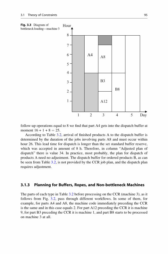
follow-up operations equal to 8 we find that part A4 gets into the dispatch buffer at
moment 16 + 1 + 8 ¼ 25.
According to Table 3.2, arrival of finished products A to the dispatch buffer is
determined by the duration of the jobs involving parts A8 and must occur within
hour 26. This lead time for dispatch is longer than the set standard buffer reserve,
which was accepted in amount of 8 h. Therefore, in column “Adjusted plan of
dispatch” there is value 34. In practice, most probably, the plan for dispatch of
products A need no adjustment. The dispatch buffer for ordered products B, as can
be seen from Table 3.2, is not provided by the CCR job plan, and the dispatch plan
requires adjustment.
3.1.3 Planning for Buffers, Ropes, and Non-bottleneck Machines
The parts of each type in Table 3.2 before processing on the CCR (machine 3), as it
follows from Fig. 3.2, pass through different workflows. In some of them, for
example, for parts A4 and A8, the machine code immediately preceding the CCR
is the same and in this case equals 2. For part A12 preceding the CCR it is machine
9, for part B3 preceding the CCR it is machine 1, and part B8 starts to be processed
on machine 3 at all.
1
2
3
4
5
6
7
8
Hour
Day1 2 3 4 5
A4
A12
B3
A8
B8
Fig. 3.3 Diagram of
bottleneck loading—machine 3
3.1 Theory of Constraints 95

The value of the buffer according to Schragenheim and Ronen (1990) should be
about three times the value of the average processing time for a lot on all machines
immediately preceding the CCR. In this case, we obtain
b ¼ 3� 4þ 1þ 2þ 1þ 0
5� 5 hour:
The CCR “rope” determines the start of the first machine in the process flow,
where the CCR is. “Rope” is activated at the moment, when the lot of parts in the
time buffer on one of the machines prior to the CCR is transferred to the CCR for
processing. Obviously, if the production is quite stable and is repeated cyclically,
then at the time of “rope” activation the production should be supplied with a new
lot of those parts that come in the buffer and wait for their turn to be processed at the
CCR. Therefore, the estimated launch of a new lot of these parts occurs earlier than
the scheduled start of processing of the current lot on the CCR by the value of the
buffer.
Assuming that machine 3 regularly processes only the parts of the above
example, then the cycle of processing is 16 h according to Fig. 3.3. Table 3.3
shows the activation moments for two cycles. For example, for part A4 according to
Fig. 3.3 the processing should be initiated at moment 12. Accordingly, start of a lot
(rope activation) must occur earlier considering the duration of stay in the buffer
equalling to 5, i.e. at moment 7.
Table 3.2 Time of dispatch in working hours
Part
code
Readiness for dispatch
(arrival to buffer)
Moment of dispatch
according to master plan
Adjusted plan of dispatch
(including buffer)
A4 25 32 34
A8 26 32 34
A12 25 32 34
B3 32 40 47
B8 39 40 47
Table 3.3 Estimated
moments of “rope”
activation for two
production cycles
Part code Activation moment, h
A4 7
A12 11
B3 13
A8 15
B8 19
A4 23
A12 27
B3 29
A8 31
B8 35
96 3 Production Bottlenecks Models
As far as the author knows, there are no practical recommendations on the size of
the required buffer of assembly and dispatch in the literature. According to various
examples cited, these values are generally within half to one working shift.
For the machines that are not the bottleneck, Schragenheim and Ronen (1990)
suggested to use the rule of greatest complexity (LPT—longest processing time)
and, if possible, not to interrupt the initiated work prior to its completion. It is
believed that in this case the possibility of unforeseen delays in the operation of the
machines that are not the bottleneck reduces, which in turn reduces the size of the
CCR buffer.
If a number of different objects, which are waiting for processing at the CCR,
can be simultaneously in the CCR buffer, then it is (Vollmann et al. 2005) often
useful to control these objects manually. To do this, the entire set of these objects is
usually divided into three zones: red, yellow, and green. The red zone should
include the objects, the processing of which according to the plan should begin
immediately or very soon. If at least one of these objects is not in the buffer, it
should immediately be an alarm with relevant organizational measures.
In the yellow zone of the buffer, the absence of some objects may be acceptable,
and necessary decisions should to be taken concerning the others. The absence of
objects in the green zone of the buffer is usually not a reason for any arrangements.
Consider a situation that may occur in the CCR buffer of our example. The
number of objects in the buffer at different times will be different. For example, at
the moment equal to 15 working hours (Fig. 3.3), as the time length of the buffer is
equal to 5 h, lots of parts A12 and B3 must be there. In this case, apparently, parts
A12 must be in the red area, i.e. mandatory, and B3 are possibly in the yellow zone.
Therefore, in the absence of parts A12 in the buffer immediate actions are required,
and for parts B3 the actions are likely advisable too.
Consider the situation with 16 h right before putting parts A12 to work on the
CCR. At this point three lots of parts must be in the buffer—A12, B3 and A8.
Obviously, not only A12, but also B3 must be in the red area, parts A8 may be either
in the yellow or green area. After putting parts A12 into operation, parts A8 should
most probably go to the yellow zone.
3.1.4 Simple Example of Theory of Constraints in Application
As a simple example of TOC application in the scheduling of discrete production
we consider the problem described in Pegels and Watrous (2005). In this chapter,
the scheduling of car lighting equipment production is considered. The bottleneck
in this production is automatic moulding machines, which produce the bodies for
lighting devices. The increase of the capacity in this case can only be achieved
through better use of working time fund of these injection moulding machines.
To produce parts of a particular nomenclature provided by the master plan the
relevant mould must be installed on the automatic moulding machine. The
machines are serviced by the maintenance team, whose correct sequence of work
eventually provides the machines operation without downtime. In fact, achieving
3.1 Theory of Constraints 97

the highest possible throughput of the production is defined by the rules of priority
when selecting a specific machine queuing for the installation of the mould. To let
the maintenance team be able to make the right choice, Pegels and Watrous (2005)
suggest to make shift-day target like it is shown in Table 3.4.
For example, for the second shift five changeovers are required—for machines
214, 210, 200, 513, and 706. If on some of these machines the previous work has
been completed and changeover is required at the same time, the question of its
sequence arises. For example, if it is required simultaneously for machines
214, 210, and 200, the priority is given to machine 214, where the complexity of
work is the highest, i.e. rule is used longest processing time or LPT (Sect. 2.3.1).
The choice of this rule is based on the intuitive assumption that since the possibility
of unforeseen delays of high complexity jobs is significantly higher, then for delays
elimination the jobs must be fulfilled as soon as possible. This example shows that
even very simple actions can have a significant effect provided the position of the
limiting resource is well identified.
3.1.5 Theory of Constraints in Process Manufacturing
Despite the fact that the theory of constraints appeared as a response to the problems
arising in the discrete production, it is quite possible to use this theory in the process
production. According to Sect. 1.3.1, the main difference between the process
production and discrete one is the ability to produce the core and by-products
simultaneously. There is one more significant difference. In the discrete production,
the size of shipment lot, transferred from one operation to another, is different from
the size of the process lot only in rare cases. The situation is just the opposite in
process production—changeover of the machines is usually performed after a
certain, often considerable, quantity of shipment lots. The dimensions of the latter
are usually determined by the size of machines or transport devices.
Table 3.4 Plan of site operation for January 20
Machine
code
Mould
type
Processing time of next
order, h
Shift number of the next order
start
112 M15 35 3
109 M20 86 1
211 M20 54 3
214 M20 125 2
210 N23 45 2
165 N23 78 3
200 P27 30 2
306 P30 44 1
513 Q50 70 2
706 Q70 71 2
98 3 Production Bottlenecks Models
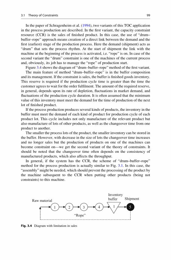
In the paper of Schragenheim et al. (1994), two variants of this TOC application
in the process production are described. In the first variant, the capacity constraint
resource (CCR) is the sales of finished product. In this case, the use of “drum–
buffer–rope” approach means creation of a direct link between the demand and the
first (earliest) stage of the production process. Here the demand (shipment) acts as
“drum” that sets the process rhythm. At the start of shipment the link with the
machine at the beginning of the process is activated, i.e. “rope” is on. In case of the
second variant the “drum” constraint is one of the machines of the current process
and, obviously, its job has to manage the “rope” of production start.
Figure 3.4 shows the diagram of “drum–buffer–rope” method of the first variant.
The main feature of method “drum–buffer–rope” is in the buffer composition
and its management. If the constraint is sales, the buffer is finished goods inventory.
This reserve is required if the production cycle time is greater than the time the
customer agrees to wait for the order fulfilment. The amount of the required reserve,
in general, depends upon its rate of depletion, fluctuations in market demand, and
fluctuations of the production cycle duration. It is often assumed that the minimum
value of this inventory must meet the demand for the time of production of the next
lot of finished product.
If the process production produces several kinds of products, the inventory in the
buffer must meet the demand of each kind of product for production cycle of each
product lot. This cycle includes not only manufacture of the relevant product but
also manufacture of lots of other products, as well as the changeover time from one
product to another.
The smaller the process lots of the product, the smaller inventory can be stored in
the buffer. However, with decrease in the size of lots the changeover time increases
and no longer sales but the production of products on one of the machines can
become constraint on—we get the second variant of the theory of constraints. It
should be noted that the changeover time often depends on the consistency of
manufactured products, which also affects the throughput.
In general, if the system has the CCR, the scheme of “drum–buffer–rope”
method for the process production is actually similar to Fig. 3.1. In this case, the
“assembly” might be needed, which should prevent the processing of the product by
the machine subsequent to the CCR when putting other products (being not
constraints) to this machine.
1 2 3
Inventory buffer
4 5
ShipmentRaw material
“Rope”
1
Fig. 3.4 Diagram with limitation in sales
3.1 Theory of Constraints 99
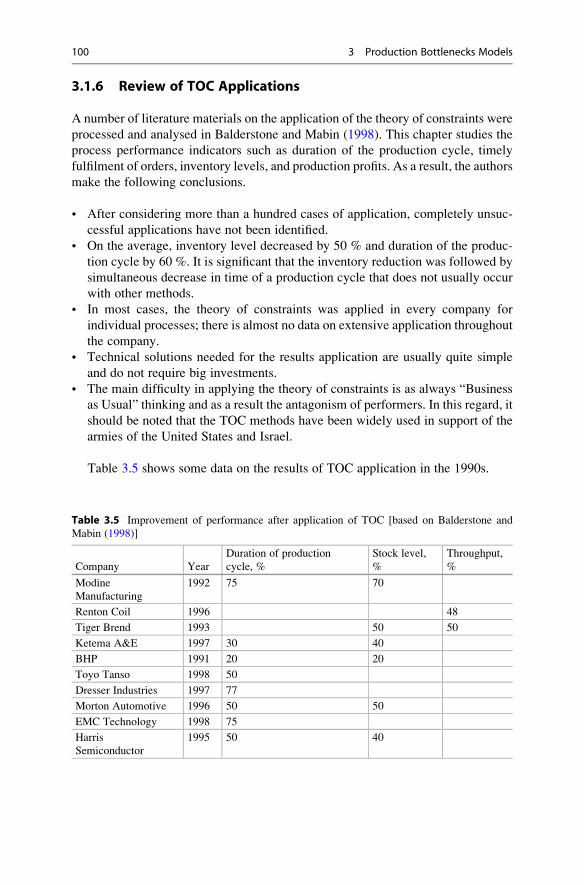
3.1.6 Review of TOC Applications
A number of literature materials on the application of the theory of constraints were
processed and analysed in Balderstone and Mabin (1998). This chapter studies the
process performance indicators such as duration of the production cycle, timely
fulfilment of orders, inventory levels, and production profits. As a result, the authors
make the following conclusions.
• After considering more than a hundred cases of application, completely unsuc-
cessful applications have not been identified.
• On the average, inventory level decreased by 50 % and duration of the produc-
tion cycle by 60 %. It is significant that the inventory reduction was followed by
simultaneous decrease in time of a production cycle that does not usually occur
with other methods.
• In most cases, the theory of constraints was applied in every company for
individual processes; there is almost no data on extensive application throughout
the company.
• Technical solutions needed for the results application are usually quite simple
and do not require big investments.
• The main difficulty in applying the theory of constraints is as always “Business
as Usual” thinking and as a result the antagonism of performers. In this regard, it
should be noted that the TOC methods have been widely used in support of the
armies of the United States and Israel.
Table 3.5 shows some data on the results of TOC application in the 1990s.
Table 3.5 Improvement of performance after application of TOC [based on Balderstone and
Mabin (1998)]
Company Year
Duration of production
cycle, %
Stock level,
%
Throughput,
%
Modine
Manufacturing
1992 75 70
Renton Coil 1996 48
Tiger Brend 1993 50 50
Ketema A&E 1997 30 40
BHP 1991 20 20
Toyo Tanso 1998 50
Dresser Industries 1997 77
Morton Automotive 1996 50 50
EMC Technology 1998 75
Harris
Semiconductor
1995 50 40
100 3 Production Bottlenecks Models
3.2 Theory of Logistic Operating Curves
Attempts to use the criteria described in Sect. 2.2.1 for optimal planning often face
their inconsistency. Indeed, the best performance criterion K4 requires to increase
the size of production lots; on the contrary, to reduce criterion K3 (cycle time) the
lot sizes should be reduced. This contradiction has been called “dilemma of
planning” (Nyhuis and Wiendahl 2009) and led to generation of a new approach
to logistics called Logistic Operating Curves Theory.
3.2.1 Production (Logistics) Variables
Logistic Operating Curves Theory considers the dependencies between the
variables describing the production process in order to establish their optimal
ratio for each particular case. For this purpose, it is necessary to describe these
variables first.
Production logistics processes are characterized by several factors: cost, the
value of work-in-progress, capacity, cycle time, and deviation from the production
plan. When constructing logistic curves some parameters can be considered as
independent variables, while others are dependent on the former. In this theory,
work-in-process (utilization rate) abbreviated as WIP is selected as an independent
variable.
This term refers to the total operation hours required to fulfil all orders in
production. It should be noted that in modern literature relating to the load manage-
ment system (see Sect. 3.5.1 below), term “workload” as a synonym for “work-in-
process” is often used. Production loading is measured in operation hours. It can
refer to a separate unit of equipment or to a workshop or an enterprise in general and
be used for all processes of production logistics.
In the general case, the job processing time (work content) for lot Qi of i-thproducts processed on i-th machine is defined as follows:
pij ¼Qiτij þ sijk
60hours; ð3:1Þ
where τij is run time per piece in min;
sijk is changeover time to i-th product form k-type product on j-type machine in
minutes.
If the changeover time does not depend on the type of product preceding i-thproduct, then index k in designation of changeover time can be omitted. Logistic
Operating Curves Theory considers mainly production processes relating to one
machine. Therefore, we will omit index j in presentation of the theory and its
applications.
Processing time for the lots with different products on the same machine is a
variable random value, which can be always defined by mean value and variance:
3.2 Theory of Logistic Operating Curves 101
p ¼ 1
n
Xni¼1
pi ð3:2Þ
and
σ2 ¼ 1
n
Xni¼1
p� pið Þ2: ð3:3Þ
Ratio of root-mean-square deviation σ to mean value
ν ¼ σ
pð3:4Þ
is called variation coefficient of processing time.
The processing time is usually measured in hours. At the same time for the
purpose of problem solution, we will need to define the time of loading the machine
in days of operation of that machine, which can be found as follows:
pi ¼pi
Pmax
working days;
and accordingly the mean value of processing time in working days
p ¼ p
Pmax
; ð3:5Þ
where Pmax is the most possible for use operation time of one machine, hours per
day. Upper limit Pmax is full working time for all shifts per day.
The third of the considered variables of the production process producing i-thproduct is duration of its cycle Fi in working days. The cycle duration is also a
random value with mean value
F ¼ 1
n
Xni¼1
Fi: ð3:6Þ
One of the basic concepts of the logistic curves theory, as well as in the TOC, is
throughput. The key to this concept is a widespread bathtub or funnel model, as
shown in Fig. 3.5.
In the model of Fig. 3.5 in the set of incoming orders going to the production
system, a queue of their consistent fulfilment forms. Then orders pass through a
hole of bathtub (funnel), which is a bottleneck of processing. In this case, the actual
capacity of equipment is always less than the maximum possible throughput.
102 3 Production Bottlenecks Models
This model resembles “drum–buffer–rope” model of the theory of constraints,
except that the latter has no “rope”. Indeed, the funnel acts as the “drum” setting the
rhythm, and the queue of accumulated orders is a buffer. The total processing time
of these orders in the buffer and directly during processing, i.e. work-in-process
(WIP), is the main independent variable in the logistic curves theory.
“Funnel” model allows describing the production capacity of any type as a set of
order input, work-in-process, and production output. The funnel neck determines
the actual output rate of the production system, which is measured in the amount of
processing time for the product output per working day. Upon entering the order,
the production is supplied with the main and auxiliary materials, components, tools,
documentation, etc., required to fulfil this order.
Logistically, the order input into production is characterized first of all by
processing time of its fulfilment. With this input, the production loading increases
abruptly by the amount of the processing time. On the other hand, when the lot of
finished products is released, the production load is reduced by the processing time
of this lot. The diagrams in Fig. 3.6 can illustrate the process of changes in the
production load associated with the orders input and production output.
Figure 3.6, which was built in the coordinates processing time p in hours—the
time t in working days, reflected changes in production loadW for time z, occurringas a result of order input I and product output O. Both at order input and product
output the production load changes abruptly by an amount corresponding to
processing time of the production lots start and release. At the end of the accounting
period z the production loadW2 may differ from the load at the beginning of period
W1. This is possible if the angle of the line, tangent of which corresponds to average
rate S of processing time change of the orders that are in production, is not equal to
the slope angle of a line of average rate of output P processing hour/working day.
Incoming orders
Set of orders
Products atbottleneck outlet
The most throughput
Current capacity
Fig. 3.5 Bathtub (funnel)
model
3.2 Theory of Logistic Operating Curves 103
Let us define the average production loadingW for period z as ratio of area A in-
between the diagrams of order input and product output to duration Z
W ¼ A=z: ð3:7ÞLet us introduce ratio R of area A to processing time O of all orders fulfilled
within period z
R ¼ A=O: ð3:8ÞAs mean output rate P, according to Fig. 3.6, is equal to
P ¼ O=z;
it is obvious that
R¼ W
P: ð3:9Þ
Expression (3.9) is called “funnel formula”. Value R (Mean WIP Range) is time
in working days which is necessary to perform mean production loading W in
processing hours at mean output rate P in hours per working day. Funnel model
presented in Fig. 3.5 allows illustrating the concept of mean coefficient of machine
work load as
p
I
2WS
O1W
Pt
z
Fig. 3.6 Diagram of
processing time flow in
production
104 3 Production Bottlenecks Models
K ¼ P=Pmax: ð3:10ÞIn the logistic curves theory, the concept of weighted mean duration of produc-
tion cycle is also used, which is defined as
Fw ¼
Xni¼1
Fipið ÞXni¼1
pi
working days: ð3:11Þ
Nyhuis and Wiendahl (2009) show that
Fw � R: ð3:12Þ
3.2.2 Some Notions Used in Queuing Theory
Theory of queue is widely used for solving the problems of orders maintaining
going through the bottleneck; at that it is supposed that order input occurs ran-
domly. This theory considers the relationship among waiting time of orders, queue
length, and machine work load coefficient.
To simplify the description the numerous existing queuing models, the classifi-
cation of these models is widely used in the form of records of type A/B/X/Y/Z. The
first two characters A and B designate kind of the probability distribution of the
time of order arrival and method for processing orders in the system. Symbol X is
the number of parallel machines processing the orders, and symbol Y describes the
capacity of these machines. Last letter Z determines the priority rules for orders
processing.
Since, for the most part, FIFO priority rule is used (Sect. 2.3.1), i.e. “First in, first
out”, and the issues of the machine capacity arise quite rarely, the first three
components in the queuing record are usually enough. When considering the
operation of one machine one of two models M/M/1 or M/G/1 is used. The first
symbol M in both of these models means that for the time of arrival the statistical
distribution of Poisson is applied. The same distribution is applicable for the first
model and order fulfilment. For the second model, the distribution of the time of
order fulfilment can vary greatly including the Poisson distribution as well.
It is to be recalled that the Poisson distribution for the orders going to the system
at mean rate λ describes probability P of receipt of n orders with time interval t asfollows
3.2 Theory of Logistic Operating Curves 105
PðnÞ ¼ ðλtÞnn!
e�λt, n ¼ 0, 1, 2, . . . ð3:13Þ
For the commonly used model M/G/1 formula of Pollaczek and Khinchine is
valid. It defines mean duration of queuing. Using this formula in terms of the above
designations of the variables gives the following expression for waiting time w
equalling the difference between the duration of production cycle F and processing
time p :
w ¼ F� p ¼ p Kð1þ ν2Þ2ð1� KÞ : ð3:14Þ
From Eq. (3.14), according to definition (3.6), it follows that the mean duration
production cycles F is more than the value of mean processing time p in working
days by the value dependent on the mean coefficient of machine loading K and
variation coefficient ν, defined by formula (3.3).
Little’s formula is very important in the theory of queues. According to this
formula the mean duration production cycle is
F ¼ N
λ; ð3:15Þ
where N is mean quantity of orders present in system; and λ is mean rate of order
receipt, i.e. quantity of orders received per day.
Nyhuis and Wiendahl (2009) clarify similarity and differences of expression
(3.15) in comparison with funnel formula (3.9). The main difference of these
dependencies is that the funnel formula uses not just the quantity of orders, like
in Little’s formula, but mean production loadingW, the value of which depends not
only on the quantity of orders but on their work content. If we evaluate the mean
production loading just as average quantity of orders in work W, which are either in
processing or waiting for it, then using expressions (3.14) and (3.15) we can obtain
W ¼ K 1þ K 1þ ν2ð Þ2 1� K� " #
: ð3:16Þ
With increase of mean machine loading K from 0 to 1 the quantity of orders
waiting for fulfilling will grow fast and become large. The length of queue for
processing according to Eq. (3.16) depends very heavily on variation coefficient ν,defined by expression (3.3). The calculations show that, e.g. increase of ν from 0.5
to 1.5 leads to increase of queue length by 1.5–2 times, and bigger increase relates
to higher values of load coefficient.
106 3 Production Bottlenecks Models
3.2.3 Plotting Logistic Operating Curves
Logistic operating curves can be constructed both for a particular unit of equipment
and the equipment group, workshop, or enterprise. In most simple cases, such
curves are constructed, for example, for one machine working independently. For
such a machine or workstation the so-called ideal logistic operating curve is
determined first.
When constructing the ideal curve the following two main assumptions are
made: (a) one order is set for processing on every machine at any given moment;
and (b) each order is fulfilled immediately after its receipt, which occurs immedi-
ately after fulfilment of the previous order. In such ideal conditions, the diagram of
changes in production load (work-in-process) with time will look like in Fig. 3.7.
Since under the assumptionsmade that in the production is always only one order,
the value of the production loadW at any time is exactly equal to the processing time
of the current order. At the same time, the duration of manufacturing under the same
conditions is also equal to the processing time. Therefore, in Fig. 3.8, each i-th orderis represented in the form of a square with a sides equal to pi.
Let us introduce the concept of ideal minimum of production loadWmin, which is
equal to average value W in the diagram. this value is equal to the area of the
diagram divided into the time of monitoring, meaning
Wmin ¼Xni¼1
pi � pið Þ=Xni¼1
pi: ð3:17Þ
Value Wmin can be calculated using the above parameters of order processing
time as follows:
Wmin ¼ p 1þ ν2�
: ð3:18Þ
W
W
ip
ip
t
Fig. 3.7 Diagram of ideal
production load [based on
Nyhuis and Wiendahl (2009)]
3.2 Theory of Logistic Operating Curves 107
Using concept Wmin we construct the so-called ideal logistic curves of mean
output rate P, mean duration of production cycle F, and mean WIP range R(Fig. 3.8).
According to Fig. 3.8 it follows that in the ideal case the mean output rate P
grows linearly with increase of mean work-in-processW to a value ofWmin, until the
processing time of the set of ideal orders is equal to the machine operation time
fund. Then P remains constant and equal to throughput Pmax. Durations F and R do
not change, while W is less than Wmin, and then increase because the orders are
put into queue for processing. Herewith as it can be illustrated, R is always bigger
than F.Real logistic curves differ from the ideal ones by the fact that instead of the break
at point Wmin the initial sections of the real curves at W < Wmin transfer smoothly
into the sections that are valid atW > Wmin. To construct a real logistic curve P its
setting in parametric form is usually used:
W ¼ Wmin 1� 1� ffiffit4
p Þ4� �
þWminα1t;�
P ¼ Pmax 1� 1� ffiffit4
p Þ4� �
:�
ð3:19Þ
Additional variable t changes from 0 to 1. It is obvious that point t ¼ 0
corresponds to the origin of coordinate and point t ¼ 1 corresponds to the point at
which the mean output rate P reaches values Pmax. Coefficient α1 determines how
much the real curve is stretched along axis W. According to a number of studies,
this coefficient is usually close to 10.
Logistic curve R is constructed according to curve P using the funnel formula
(3.9). To construct logistic curve F the following relation is used:
P hours/work. day
F, R maxP working days
PR
FminW W hours
Fig. 3.8 Ideal logistic curves
[based on Nyhuis and
Wiendahl (2009)]
108 3 Production Bottlenecks Models
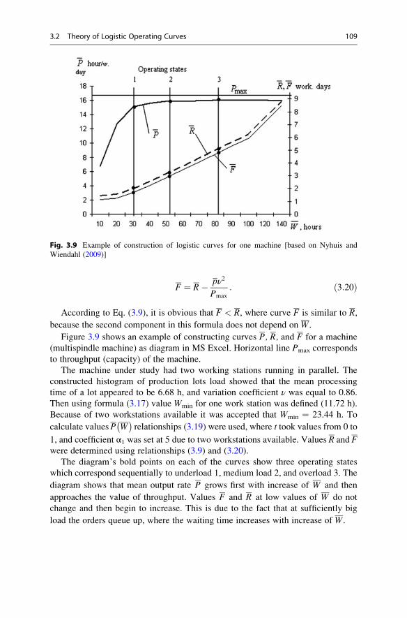
F ¼ R� pν2
Pmax
: ð3:20Þ
According to Eq. (3.9), it is obvious that F < R, where curve F is similar to R,
because the second component in this formula does not depend on W.
Figure 3.9 shows an example of constructing curves P, R, and F for a machine
(multispindle machine) as diagram in MS Excel. Horizontal line Pmax corresponds
to throughput (capacity) of the machine.
The machine under study had two working stations running in parallel. The
constructed histogram of production lots load showed that the mean processing
time of a lot appeared to be 6.68 h, and variation coefficient ν was equal to 0.86.
Then using formula (3.17) value Wmin for one work station was defined (11.72 h).
Because of two workstations available it was accepted that Wmin ¼ 23.44 h. To
calculate valuesP W�
relationships (3.19) were used, where t took values from 0 to
1, and coefficient α1 was set at 5 due to two workstations available. Values R and Fwere determined using relationships (3.9) and (3.20).
The diagram’s bold points on each of the curves show three operating states
which correspond sequentially to underload 1, medium load 2, and overload 3. The
diagram shows that mean output rate P grows first with increase of W and then
approaches the value of throughput. Values F and R at low values of W do not
change and then begin to increase. This is due to the fact that at sufficiently big
load the orders queue up, where the waiting time increases with increase of W.
Fig. 3.9 Example of construction of logistic curves for one machine [based on Nyhuis and
Wiendahl (2009)]
3.2 Theory of Logistic Operating Curves 109

3.2.4 Main Properties of Logistic Curves
The following are details of some properties of logistic operating curves. Under-
standing of the properties described increases significantly the opportunities of
application of these curves to control bottleneck operation.
The most important and equally rather obvious feature is the balancing of order
input and product output processes in due course. These processes are described by
stepped curves in Fig. 3.6. Accordingly, input rate S on a sufficiently long time
interval usually corresponds to mean output rate P.
As was shown above, such characteristics of logistic curves as timeR required to
perform mean work-in-process W at mean output rate P, as well as duration of the
production cycle F, are directly dependent on ratio W/P.
Changing of machine load coefficient K influences greatly both production load
W and duration of the cycle F. With heavy loaded equipment, even relatively small
reduction of K can seriously reduce load W. Since in the real conditions, big
fluctuations in production loads are often observed, then a buffer is necessary to
stabilize high load equipment. As you can see, this property actually repeats the
suggestion of using the buffer in the Theory of Constraints (Sect. 3.1.1).
Mean duration of the production cycle F can seriously be influenced by the
established priority rule in fulfilment of orders (Sect. 2.3.1). Generally speaking, the
minimum durationF occurs when the rule of “first in, first out” (FIFO) is applied. It
should be borne in mind that increase in the cycle time difference, when instead of
FIFO, for example, rules SPT or LPT are used, depends on the processing time
dispersion. The more is the variation in the processing time of the individual jobs,
the more significant increase in the mean duration of the cycle.
3.3 Application of Logistic Operating Curves
Theory of logistic curves enables to carry out various improvements of the produc-
tion process. Mostly, these improvements are carried out to reduce current produc-
tion load W. It is possible to decrease W due to the rational planning in particular,
where the processing time of the individual jobs is equalled as much as possible. In
general, the greatest effect of the logistics operating curves can be seen in their use
for the so-called logistic positioning and bottleneck analysis.
3.3.1 Logistic Positioning
The purpose of logistic positioning is to determine the most appropriate ratio in a
given situation between such contradictory process indicators as its duration F and
machine load coefficient K. Let us demonstrate the meaning of the logistic posi-
tioning by the example of logistic curves P, R, and F in Fig. 3.9.
110 3 Production Bottlenecks Models
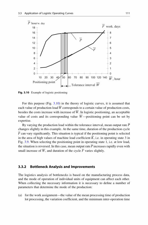
For this purpose (Fig. 3.10) in the theory of logistic curves, it is assumed that
each value of production loadW corresponds to a certain value of production costs,
besides the costs increase with increase ofW. In logistic positioning, an acceptable
value of costs and its corresponding value W—positioning point can be set by
expertise.
By varying the production load within the tolerance interval, mean output rate Pchanges slightly in this example. At the same time, duration of the production cycle
F can vary significantly. This situation is typical if the positioning point is selected
in the area of high values of machine load coefficient K, i.e. in operating state 3 in
Fig. 3.9. When selecting the positioning point in operating state 1, i.e. at low load,
the situation is reversed. In this case, mean output rateP increases rapidly even with
small increase of W, and duration of the cycle F varies slightly.
3.3.2 Bottleneck Analysis and Improvements
The logistics analysis of bottlenecks is based on the manufacturing process data,
and the mode of operation of individual units of equipment can affect each other.
When collecting the necessary information it is necessary to define a number of
parameters that determine the mode of the production:
(a) for the work assignment—the value of the mean processing time of production
lot processing, the variation coefficient, and the minimum inter-operation time
0
2
4
6
8
10
12
14
16
18
10 20 30 40 50 60 70 80 90 100 120 1400
1
2
3
4
5
6
7
8
P hour/w. day
W , hour
P
F
F work. days
Tolerance interval WPositioning point
Fig. 3.10 Example of logistic positioning
3.3 Application of Logistic Operating Curves 111
(b) for the production cycle duration—the mean value, the variation coefficient
and the mean value of the time for production load performance
(c) for production rate—the average value in hours per day and the number of
fulfilled orders
(d) for the work-in-process—the mean value in hours and number of orders
(e) to analyse the schedule adherence—relative delay and its variation coefficient
During the analysis, various logistic targets have to be defined, which can
sometimes be inconsistent. The starting point for establishing the target priority is
the logistic positioning described above. Actually, this means the determination of
what is most important in the current situation—mean output rate P or cycle
duration F.Bottlenecks in the production flow cause an increase in the production cycle
duration F, so it is natural to tend to reduce this value somehow. Methods of
bottleneck “pointing” are well known, but here it is reasonable to consider them in
terms of logistics analysis. Naturally, the increase of the maximum throughput Pmax
(at least temporary) is the most effective. If it is not possible, you should delay the
order transferring for processing, if practical. In this case, the mean value of
production load W reduces, and, as it follows from Fig. 3.10, duration of the
cycle F can reduce.
More complex methods of influencing the equipment performance, which is the
“bottleneck”, are based on the so-called harmonization of orders. First of all, it is an
attempt to reduce the spread of the processing time of production lots and, there-
fore, to reduce the variation coefficient ν. Value ν, pursuant to formula (3.18),
influences greatly the ideal minimum of production load Wmin, which in turn,
according to expression (3.19), leads to a significant decrease of the mean produc-
tion load W.
Besides,Wmin essentially depends on the mean processing time of the production
lot p (Eq. 3.18) and the sizes of the lots can be reduced in extreme cases. Of course,
such method for accelerating the order fulfilment leads to an increase in setup time
and, in general, an increase in the labour input and it should be used with caution.
From this perspective, it is advisable not only to reduce the size of a production lot
supplied for processing but also to distinguish between the sizes and quantity
number of input lots and output lots. This can reduce the bottleneck’s effect on
the business greatly in many cases.
3.3.3 Evaluation of Overall Production Performance
In the framework of the logistic curves theory, we can construct a logistic curve
describing the efficiency of a production process both for a single machine and for
the whole enterprise. To do this, we use mean production loadW as an independent
variable of the process, which is usual for this theory. Efficiency of the process is
characterized by the following basic parameters. Firstly, it is cost characteristics—
112 3 Production Bottlenecks Models
income received as a result of the production load performance and production
costs for time of the production load performance. Secondly, the efficiency of
operation is essentially determined by the load level of the equipment available at
the enterprise. Finally, the evaluation of the operation quality depends on the ability
of the enterprise to fulfil the received orders in time.
Let us introduce the complex criterion of production process efficiency
E ¼ f K
cH; ð3:21Þ
where f is profit for time R of production load performance,
c is production costs for that period,
K is mean coefficient of the equipment utilization, and
H is mean intensity of obligations performance under the contracts with
consumers.
Criterion E allows consideration of several aspects of production activity simul-
taneously: profitability, capacities utilization, and real possibilities to perform
contractual obligations.
Taking into account that the profit is equal to the difference of sales G and costs,
then formula (3.21) will look as follows:
E ¼ G=C� 1ð ÞKH:
ð3:22Þ
All the components in expression (3.22) depend on value of production loadW.
WhenW¼ 0, meaning there are no orders for products, the value of profit is 0, and
the value of costs is not equal to 0, as the costs are required to support the enterprise
activity. Machine load coefficient is also equal to 0, and to calculate the value of
criterion E it is required to define value H.It has to be recalled that the concept of intensity Hi for i-th order, introduced in
Sect. 2.4.1 by formula (2.23), for the case when the delivery time is not over yet, is
defined as
Hi ¼ T1i þ T2ið Þ=z1i;where T1i is a component defined by the processing time not performed at the
moment of scheduling;
T2i is a component appeared due to necessity of transferring of job to the
remaining operations;
z1i is the estimated production time reserve against to the target.
This intensity is variable in time and can be determined for any moment of the
actual fulfilment of an order. However, to assess the overall effectiveness of
production there is no need to rely on the intensity of each order. For this purpose,
it makes sense to determine the mean intensity as follows
3.3 Application of Logistic Operating Curves 113
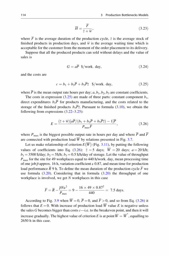
H ¼ F
zþ w, ð3:23Þ
where F is the average duration of the production cycle, z is the average stock of
finished products in production days, and w is the average waiting time which is
acceptable for the customer from the moment of the order placement to its delivery.
Suppose that all the produced products can sold without delays and the value of
sales is
G ¼ aP $=work: day, ð3:24Þand the costs are
c ¼ b1 þ b2Pþ b3Pz $=work: day, ð3:25Þwhere P is the mean output rate hours per day; a, b1, b2, b3 are constant coefficients.
The costs in expression (3.25) are made of three parts: constant component b1,
direct expenditures b2P for products manufacturing, and the costs related to the
storage of the finished products b3Pz. Pursuant to formula (3.10), we obtain the
following from expressions (3.22–3.25):
E ¼ ðzþ wÞ½aP=ðb1 þ b2Pþ b3PzÞ � 1�PPmaxF
, ð3:26Þ
where Pmax is the biggest possible output rate in hours per day and where P and F
are connected with production load W by relations presented in Fig. 3.7.
Let us make relationship of criterion E W�
(Fig. 3.11), by putting the following
values of coefficients into Eq. (3.26): z ¼ 5 days; W ¼ 20 days; a¼ 20 $/h;
b1¼ 3500 $/day; b2¼ 5$/h; b3¼ 0.5 $/h/day of storage. Let the value of throughput
Pmax for the site for 49 workplaces equal to 440 h/work. day, mean processing time
of one job p approx. 16 h, variation coefficient ν 0.87, and mean time for production
load performance R 9 h. To define the mean duration of the production cycle F we
use formula (3.20). Considering that in formula (3.20) the throughput of one
workplace is involved, we get N workplaces in this case
F ¼ R� pNν2
Pmax
¼ 9� 16� 49� 0:872
440¼ 7:5 days:
According to Fig. 3.9 when W ¼ 0, P¼ 0, and F> 0, and so from Eq. (3.26) it
follows that E¼ 0. With increase of production load W value E is negative unless
the salesG becomes bigger than costs c—i.e. to the breakeven point, and then it will
increase gradually. The highest value of criterion E is at pointW ¼ W*, equalling to
2650 h in this case.
114 3 Production Bottlenecks Models
Let us consider the change in the intensity value for various values of z and w.For the values set for the construction of the curve in Fig. 3.11
H ¼ F
zþ w¼ 7:5
5þ 20¼ 0:3:
Average waiting time w, which is acceptable for the customer, essentially
depends on the type of market conditions, which were described in Sect. 1.6.1.
With the growing market, the customer is usually willing to wait long enough and
value w can be comparable to or even exceed duration of the production cycle F. In
this case, intensity H is small and can reduce the number of working days z of
warehouse stock to 0. On the stable market, the acceptable waiting time is deter-
mined by the competition and usually requires some or sometimes a substantial
margin.
When operating on the mature market, there are large fluctuations in the flow of
orders, and not to lose an order its fulfilment should be provided fast enough. At the
same time, under these conditions, it is not economically justified to store large
amounts, since it is difficult to predict when they are demanded. In addition, large
fluctuations in demand lead to an increase in the duration of the production cycleF,which also leads to an increase in intensity and reduction of effectiveness E.
Under these conditions, transition from the strategy “make-to-order” to strategy
“assembly-to-order” should be considered as the main way to enhance efficiency.
Using this strategy can dramatically reduce fluctuations in production load W,
reduce cycle time and intensity, and ultimately, raise the value of efficiency
criterion E.
Fig. 3.11 Curve of efficiency complex criterion
3.3 Application of Logistic Operating Curves 115

3.4 Optimal Lot Sizing for Production Bottlenecks
In the literature on the production scheduling, a simple formula is often
recommended, which determines the lot size Qi for the i-type product as the
minimum allowable for the high load equipment:
Qi ¼si 1� δð Þ
τiδ; ð3:27Þ
where si, τi, like in expression (3.1), are setup time and processing time per piece,
accordingly, and δ is a norm coefficient of acceptable loss of time for changeover.
Since formula (3.27) does not take into account the value of demand Di for the
manufactured product, Karmarkar et al. (1992) suggested to perform the so-called
approximate calculation of a lot
Qi ¼ φDi; ð3:28Þusing other norm coefficient φ, defining the ratio of a lot size to some, e.g. annual,
demand.
Formulas (3.27) and (3.28) are vague because of the uncertainty of norm
coefficients. There are other difficulties with the application. For example, it is
difficult to set the demand horizon; even when these formulas can be used the
difference in two values obtained may be so big that the actual lot sizing becomes
difficult, etc.
At the same time, wide application of these relationships suggests two things.
Firstly, there is a serious need for a method of calculating the lot size, taking into
account the equipment load level. Secondly, this method should use production
process parameters that are used in expressions (3.27) and (3.28). In the 1990s, a
series of studies were made aimed at the development of this method, and the
results in the studies of Karmarkar et al. (1992) set forth in the following paragraph
received the greatest recognition.
3.4.1 Lot Sizing Heuristic
The methods discussed here are based on the fact that the waiting for processing is
usually a large part of the production cycle duration. This leads to an increase of
lead time inventories, to lengthening of time for order fulfilment, etc., and therefore
it is quite useful to reduce the waiting time for processing. The reduced waiting time
is usually associated with the reduced size of production lots, but with too small lots
the average waiting time in the queue may increase due to the increasing time loss
of setups. Therefore, it makes sense to try to calculate such lot sizes, which provide
mathematical minimum of the mean waiting time.
Mean waiting time w, in terms of Karmarkar et al. (1992) approach, which
considers processing queues in the framework of M/G/1 model described in
116 3 Production Bottlenecks Models
Sect. 3.2.2, is a function of vectorQ (set of values) of lotsQi of various i-th productsthat must undergo processing on the same machine. Value w Qð Þ is inherently equalto the difference of mean cycle time F and mean value of processing time p in
working days.
The basis for the described approach is formula (3.14) of Pollaczek and
Khinchine, given above in Sect. 3.2.2, for mean waiting time w Qð Þ. After some
transformations, the formula is given by
w Qð Þ ¼ λE p2ð Þ2 1� K� : ð3:29Þ
In formula (3.29),K is still coefficient of load, E( p2) is mean value of the square
of processing time p2, and value λ, the same as above in Sect. 3.2.2, represents the
rate of order arrival for processing. Here this rate is define as follows
λ ¼Xni¼1
λi ¼Xni¼1
Di
Qi
; ð3:30Þ
meaning λ is the total number of all lots n of different products coming within the
time, for which the demand is established. To be specific, we assume that the
production intensity is equal to demand Di and is defined in the pcs/h.
The time for performance of one job (lot) pi in hours is defined as a function of
lot size Qi
pi ¼ si þ Qi
Pi; ð3:31Þ
where, as above, si is the setup time in hours and Pi is the machine capacity in pcs/h.
Whereas the probability of arrival of i-th product lot is equal to
Pi ¼ λi=λ, ð3:32Þtime of processing of random value pi has discrete distribution with mean value
p ¼ EðpÞ ¼Xni¼1
Pipi: ð3:33Þ
From expressions (3.30–3.33) it follows that the mean coefficient of load is equal
to
K ¼ λp: ð3:34ÞThe so-called second-order moment of the random discrete value pi, which is
used in formula (3.29), is defined as
3.4 Optimal Lot Sizing for Production Bottlenecks 117
Eðp2Þ ¼Xni¼1
Pip2i : ð3:35Þ
Since the purpose of this problem is to determine the optimal lot sizes, all the
values appearing in expression (3.29) are inserted into (3.29) as functions from Qi.
The problem under consideration is formulated mathematically as finding the
minimum waiting time
w* ¼ minQi>0
w Qð Þ ð3:36Þ
at multiple values of Qi with constraints
Xni¼1
Di=Pi þ Disi=Qið Þ < 1; ð3:37Þ
meaning that load coefficient K must be less than one.
From expressions (3.31–3.35), we can obtain
w Qð Þ ¼
Xni¼1
Di
Qi
si þ Qi
Pi
� �2
2�1�
Xni¼1
Di
Qi
si þ Qi
Pi
� � :
ð3:38Þ
To find the minimum of function w Qð Þ for each variable Qi, it is necessary to
define the partial derivative with respect to this variable and set it equal to zero.
Since all the equations for each variable have the same form, it is sufficient to solve
one of them. The most compact form of this equation is represented by Kuik and
Tielemans (1998)
Xni¼1
ui
ffiffiffiffiffiffiffiffiffiffiffiffiffiffiffiffiffiffiffiffiffis2i þ 2siw
*q
¼ 1� uð Þw* �Xni¼1
uisi; ð3:39Þ
where the operation load (without time for setup) of machine u is a combination of
lot processing load of each i-type product
u ¼Xni¼1
ui ¼Xni¼1
Di
Pi: ð3:40Þ
Equation (3.39) includes the optimal value of mean waiting time w*, which is
associated with the relevant optimal values Qi by expression (3.38). Hence, it
follows that the value for one i-th product Qi cannot be found separately from
118 3 Production Bottlenecks Models
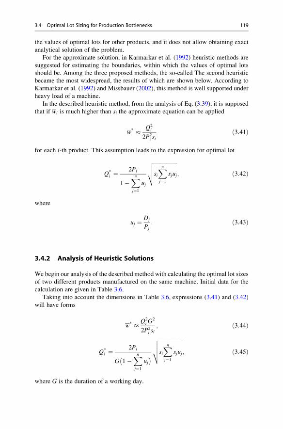
the values of optimal lots for other products, and it does not allow obtaining exact
analytical solution of the problem.
For the approximate solution, in Karmarkar et al. (1992) heuristic methods are
suggested for estimating the boundaries, within which the values of optimal lots
should be. Among the three proposed methods, the so-called The second heuristic
became the most widespread, the results of which are shown below. According to
Karmarkar et al. (1992) and Missbauer (2002), this method is well supported under
heavy load of a machine.
In the described heuristic method, from the analysis of Eq. (3.39), it is supposed
that if wi is much higher than si the approximate equation can be applied
w* � Q2i
2P2i si
ð3:41Þ
for each i-th product. This assumption leads to the expression for optimal lot
Q*i ¼
2Pi
1�Xnj¼1
uj
ffiffiffiffiffiffiffiffiffiffiffiffiffiffiffiffiffiffisiXnj¼1
sjuj
vuut ; ð3:42Þ
where
uj ¼ Dj
Pj: ð3:43Þ
3.4.2 Analysis of Heuristic Solutions
We begin our analysis of the described method with calculating the optimal lot sizes
of two different products manufactured on the same machine. Initial data for the
calculation are given in Table 3.6.
Taking into account the dimensions in Table 3.6, expressions (3.41) and (3.42)
will have forms
w* � Q2i G
2
2P2i si
; ð3:44Þ
Q*i ¼
2Pi
G�1�
Xnj¼1
uj
ffiffiffiffiffiffiffiffiffiffiffiffiffiffiffiffiffiffisiXnj¼1
sjuj
vuut ; ð3:45Þ
where G is the duration of a working day.
3.4 Optimal Lot Sizing for Production Bottlenecks 119
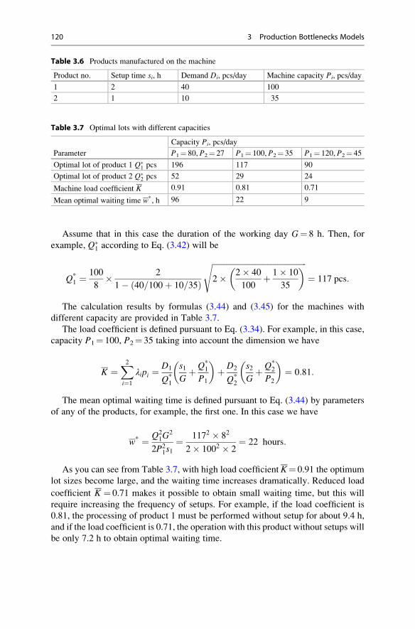
Assume that in this case the duration of the working day G¼ 8 h. Then, for
example, Q1 according to Eq. (3.42) will be
Q*1 ¼
100
8� 2
1� 40=100þ 10=35ð Þ
ffiffiffiffiffiffiffiffiffiffiffiffiffiffiffiffiffiffiffiffiffiffiffiffiffiffiffiffiffiffiffiffiffiffiffiffiffiffiffiffiffiffiffiffiffiffiffiffi2� 2� 40
100þ 1� 10
35
� �s¼ 117 pcs:
The calculation results by formulas (3.44) and (3.45) for the machines with
different capacity are provided in Table 3.7.
The load coefficient is defined pursuant to Eq. (3.34). For example, in this case,
capacity P1¼ 100, P2¼ 35 taking into account the dimension we have
K ¼X2i¼1
λipi ¼D1
Q*1
s1Gþ Q*
1
P1
� �þ D2
Q*2
s2Gþ Q*
2
P2
� �¼ 0:81:
The mean optimal waiting time is defined pursuant to Eq. (3.44) by parameters
of any of the products, for example, the first one. In this case we have
w* ¼ Q21G
2
2P21s1
¼ 1172 � 82
2� 1002 � 2¼ 22 hours:
As you can see from Table 3.7, with high load coefficient K¼ 0.91 the optimum
lot sizes become large, and the waiting time increases dramatically. Reduced load
coefficient K ¼ 0.71 makes it possible to obtain small waiting time, but this will
require increasing the frequency of setups. For example, if the load coefficient is
0.81, the processing of product 1 must be performed without setup for about 9.4 h,
and if the load coefficient is 0.71, the operation with this product without setups will
be only 7.2 h to obtain optimal waiting time.
Table 3.6 Products manufactured on the machine
Product no. Setup time si, h Demand Di, pcs/day Machine capacity Pi, pcs/day
1 2 40 100
2 1 10 35
Table 3.7 Optimal lots with different capacities
Parameter
Capacity Pi, pcs/day
P1¼ 80, P2¼ 27 P1¼ 100, P2¼ 35 P1¼ 120, P2¼ 45
Optimal lot of product 1 Q1 pcs 196 117 90
Optimal lot of product 2 Q2 pcs 52 29 24
Machine load coefficient K 0.91 0.81 0.71
Mean optimal waiting time w*, h 96 22 9
120 3 Production Bottlenecks Models

Now, we consider the nature of the ratio between the optimal lot sizes of various
products. Using expression (3.42), we obtain
Q*i
Q*k
¼ Pi
Pk
ffiffiffiffiffisisk:
rð3:46Þ
From Eq. (3.46) it follows that the optimal ratio between the optimal lots does
not depend on the machine load, i.e. the size of demand Di. In this case, for
example, the ratio between capacities P1 and P2 varies in a small range—from
2.7 to 3.0. Therefore, the ratio of the optimal lots, as can be seen from Table 3.7,
changes slightly as well—from 3.7 to 4.0.
The results presented in the previous paragraph also determine the direction, in
which it is advisable to work on reduction of the setup time. For example, if it is
decided to develop relevant devices that accelerate the setup, it makes sense to
determine for which type of the products the setup time reduction is more effective.
This question has been studied in detail in the paper of Kuik and Tielemans (1998).
Obviously, in the case where, for example, the setup time for the i-th product
affects the changes in the mean waiting time w more than the time of setup for
k-type product, the following condition shall be satisfied:
∂w∂si
>∂w∂sk
; ð3:47Þ
i.e. the partial derivative from the waiting time for the i-th product shall be bigger
than for the k-type product. Since with the equality of these derivatives there is the
same effect of both products, so for the solution of this problem it is necessary to
define a set of parameters of the problem corresponding to this equation—the
so-called indifference curve.
In Kuik and Tielemans (1998), the indifference curve is defined as function
ui ¼ ϕ uk; si; skð Þ; ð3:48Þwhere ui, uk are variables defined by expression (3.43).
Analysis of the results of Kuik and Tielemans (1998) paper shows that functions
(3.46) depend little on the setup time, in most cases, i.e. the indifference curve may
be replaced by a straight line without prejudice for practical use
ui ¼ uk: ð3:49ÞFigure 3.12 shows the indifference line for the example with data in Table 3.6.
Since point A with coordinates u1¼ 0.4; u2¼ 0.28, corresponding to the process
state in Table 3.6, is below the indifference line, then the reduction in setup time for
product 1 affects the mean wait time more than a similar decrease in setup time for
product 2. Table 3.8 presents three possible combinations of setup time for products
from Table 3.6. Data from Table 3.8 show that setup time reduction for the first
3.4 Optimal Lot Sizing for Production Bottlenecks 121
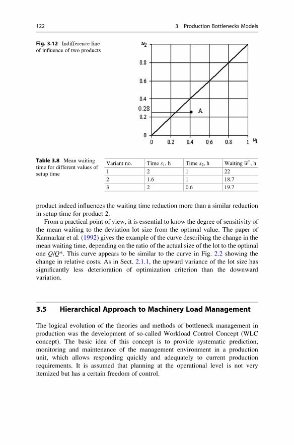
product indeed influences the waiting time reduction more than a similar reduction
in setup time for product 2.
From a practical point of view, it is essential to know the degree of sensitivity of
the mean waiting to the deviation lot size from the optimal value. The paper of
Karmarkar et al. (1992) gives the example of the curve describing the change in the
mean waiting time, depending on the ratio of the actual size of the lot to the optimal
one Q/Q*. This curve appears to be similar to the curve in Fig. 2.2 showing the
change in relative costs. As in Sect. 2.1.1, the upward variance of the lot size has
significantly less deterioration of optimization criterion than the downward
variation.
3.5 Hierarchical Approach to Machinery Load Management
The logical evolution of the theories and methods of bottleneck management in
production was the development of so-called Workload Control Concept (WLC
concept). The basic idea of this concept is to provide systematic prediction,
monitoring and maintenance of the management environment in a production
unit, which allows responding quickly and adequately to current production
requirements. It is assumed that planning at the operational level is not very
itemized but has a certain freedom of control.
Fig. 3.12 Indifference line
of influence of two products
Table 3.8 Mean waiting
time for different values of
setup time
Variant no. Time s1, h Time s2, h Waiting w*, h
1 2 1 22
2 1.6 1 18.7
3 2 0.6 19.7
122 3 Production Bottlenecks Models

3.5.1 Principles of Workload Control Concept
TheWLC concept provides two basic methods of such control (Henrich et al. 2003):
• Creation of buffers protecting from fluctuations in production load
• Aggregation of jobs and equipment into groups
Sets of jobs grouped by any ground together are called “workload” in terms of
this concept. The WLC concept is expected to provide quite small cycle time by
adjusting workloads within certain established norms. At the same time, such
regulation should ensure the timely execution of jobs in accordance with the
existing contracts. For this purpose, the software supporting the WLC concept
should enable the acceptance of orders and determine their due dates and start dates.
In theory, this concept is based on the logistic relationship between production
load W and duration of the production cycle F, described in Sect. 3.2.1. According
to this relationship, when the production load is within the established norms, the
duration of the cycle will also be within acceptable limits.
To make the load control possible, it is detailed. For this purpose, first of all,
it is assumed that in the unit (shop) the operation is performed in two levels. The
first is the level of accounting, planning, and delivery of incoming jobs (pool), and
then it is the level of the performers (shop floor). Accordingly, the total production
load, which must be performed on the j-type work center, is divided into two
components, Wpj and Wf
j . Each of these components has its own duration Fpj and
Ffj . Moreover, when more precise control is needed, the load of performers Wf
j can
be divided into the load being performed in the current time period, waiting for
performance and already performed. These loads can be associated with the
corresponding durations of the process and checked for their compliance with
standards in place.
Figure 3.13 shows the hierarchical control scheme at the shop floor level in the
described concept by Land (2004). The circles in the diagram designate machines
and the rectangles designate buffers. The material flows are indicated by bold
arrows and the control lines are indicated by regular arrows. Material feed into
the pool, from the pool to the work center B pool and the latter to processing are
controlled by the hierarchical system of load shown in the upper part of Fig. 3.13.
This system allows controlling both the material flow input and product output from
processing and adjust the outgoing flow by changing the capacity of the equipment.
The decisions made at the level of the job input are used to control the entire
volume of the gained load. The start level controls the load of work centers, and the
level of scheduling allows setting the priority of each job.
The main purpose of the controlled load concept is to maintain minimal loaded
condition at the level of lean shop floor. When controlling by the scheme showed in
Fig. 3.13, the job does not accumulate in queues (logjam) before work centers and
does not compete for the right of processing, but wait for the start in the workshop
3.5 Hierarchical Approach to Machinery Load Management 123
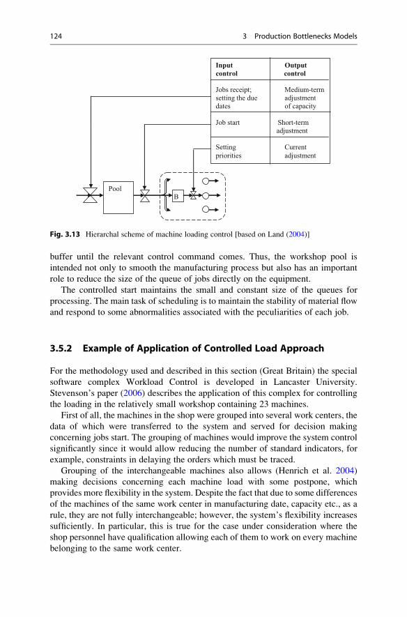
buffer until the relevant control command comes. Thus, the workshop pool is
intended not only to smooth the manufacturing process but also has an important
role to reduce the size of the queue of jobs directly on the equipment.
The controlled start maintains the small and constant size of the queues for
processing. The main task of scheduling is to maintain the stability of material flow
and respond to some abnormalities associated with the peculiarities of each job.
3.5.2 Example of Application of Controlled Load Approach
For the methodology used and described in this section (Great Britain) the special
software complex Workload Control is developed in Lancaster University.
Stevenson’s paper (2006) describes the application of this complex for controlling
the loading in the relatively small workshop containing 23 machines.
First of all, the machines in the shop were grouped into several work centers, the
data of which were transferred to the system and served for decision making
concerning jobs start. The grouping of machines would improve the system control
significantly since it would allow reducing the number of standard indicators, for
example, constraints in delaying the orders which must be traced.
Grouping of the interchangeable machines also allows (Henrich et al. 2004)
making decisions concerning each machine load with some postpone, which
provides more flexibility in the system. Despite the fact that due to some differences
of the machines of the same work center in manufacturing date, capacity etc., as a
rule, they are not fully interchangeable; however, the system’s flexibility increases
sufficiently. In particular, this is true for the case under consideration where the
shop personnel have qualification allowing each of them to work on every machine
belonging to the same work center.
PoolB
Input Outputcontrol control
Jobs receipt; Medium-termsetting the due adjustmentdates of capacity
Job start Short-termadjustment
Setting Current
priorities adjustment
Fig. 3.13 Hierarchal scheme of machine loading control [based on Land (2004)]
124 3 Production Bottlenecks Models
In the illustrated case, all the machines were divided into 12 work centers with
1–4 machines in each center. Interchangeability of the machines in one work center
averaged about 80 %. Then for each work center, its capacity was determined. The
capacity was determined based on the number of employees, their classification,
and the possibility to work in different shifts and overtime. At the same time, the
possible transfer of employees from one work center to another in accordance with
their qualifications is analysed.
After that, the average performance of the work center per 1 h of work by an
employee is calculated. For example, for one of the work centers this indicator
amounted to 1.5 processing hour per 1 h of an employee’s working time. This
indicator, as well as time real resources of the employees, was monitored by the
system on a regular basis.
After the above preparation, the system allowed users to control loads in the
following modes:
• Customers’ requests control
• Introduction of new jobs
• Launching of jobs in production
• Capacities control
• Loads scheduling
To evaluate the effectiveness of the system activity, the performance indicators
with a set of quite standing orders of one customer were studied. The orders
accounted for about 10 % of the total work content of production. This evaluation
was performed in three directions:
• Changes in the data structure on consumers’ requests
• Changes in the scheduling
• Changes in the nature of delays of orders
Usage of the system showed that there is a significant difference in the percep-
tion of the quality of receiving orders from the company management and the
customer. While the management believes that only 15 % of the customer’s
requirements is not met, the customer believes the percentage is equal to 85.
Consequently, measures had been taken to consider the customer’s requirements
to the full.
During scheduling, it was found that when allocating jobs from the date of
completion required under the contract by reverse calculation up to the present
moment, it often appears that the lead time or capacity is not enough. Sometimes,
there are situations when the required date appears to pass already at the moment of
data input.
For correct calculation in scheduling as early as the stage of due date negotiation,
the standards were used for the jobs queuing to the work center and the duration of
the presence of the jobs in the workshop buffer. In such cases, the system helped to
hold additional negotiations to adjust the due dates. The study of order delays nature
3.5 Hierarchical Approach to Machinery Load Management 125
revealed the need to monitor performance daily, when the duration of the produc-
tion cycle is quite small. Otherwise, it is possible to do weekly check of the order
status.
References
Balderstone, S. J., & Mabin, V. J. (1998). A review of Goldratt’s Theory of Constraints (TOC) –lessons from the international literature. www.speed4projects.net/. . ./1998
Goldrat, E. (1987). Computerized shop floor scheduling. International Journal of ProductionResearch, 26, 443–455.
Henrich, P., Land, M. J., Gaalman, G., & Van Der Zee, D. J. (2003). The effect of information on
workload control. In First Joint EUROMA POMS Conference Proceedings (pp. 611–620).Henrich, P., Land, M. J., & Gaalman, G. (2004). Grouping machines for effective workload
control. In 13th International Working Seminar on Production Economics ConferenceProceedings (Vol. 4, pp. 141–160).
Karmarkar, U. S., Kekre, S., & Kekre, S. (1992). Multi-item batching heuristics for minimization
of queueing delays. European Journal of Operational Research, 58, 99–111.Kuik, R., & Tielemans, P. F. (1998). Analysis of expected queueing delays for decision making in
production planning. European Journal of Operational Research, 110, 658–681.Land, M. J. (2004).Workload control in job shops, grasping the tap. http://dissertations.ub.rug.nl/
faculties/management/2004/m.j.land
Missbauer, H. (2002). Lot sizing in workload control systems. Production Planning & Control, 13,649–664.
Nyhuis, P., & Wiendahl, H.-P. (2009). Fundamentals of production logistic. Berlin: Springer.Pegels, C. C., & Watrous, C. (2005). Application of the theory of constraints to a bottleneck
operation in a manufacturing plant. Journal of Manufacturing Technology Management, 16,302–311.
Schragenheim, E., Cox, J., & Ronen, B. (1994). Process flow industry – scheduling and control
using theory of constraints. International Journal of Production Research, 32, 1867–1877.Schragenheim, E., & Ronen, B. (1990). Drum-buffer-rope shop floor control. Production and
Inventory Management Journal, Third Quarter, 18–22.Stevenson, M. (2006). Refining a Workload Control (WLC) concept: a case study. International
Journal of Production Research, 44, 767–790.Vollmann, T. E., Berry, W. L., Whybark, D. C., & Jacobs, F. R. (2005). Manufacturing planning
and control for supply chain management. Boston: McGrawHill.
126 3 Production Bottlenecks Models

Multi-criteria Models and Decision-Making 4
4.1 Basic Concepts in Multi-criteria Optimization Theory
This theory aims to develop an optimal solution of the complicated problem under
the conditions where there is no one clear criterion for the quality of such solution.
In the theory of multi-criteria optimization, the decision methods are being devel-
oped to adequately reconcile various criteria that are important from the point of
view of the decision-maker (DM). The full range of these methods can be condi-
tionally divided into two groups:
• Methods of finding a decision
• Methods of decision support
While in the first case the decision is completely determined in the framework of
the theory, in the second case, the theory only suggests possible decisions to the
DM, leaving the right of choice to DM. In reality, multi-criteria optimization
methods always contain the elements of both these approaches to any extent.
4.1.1 Definition of Multi-criteria Optimization Problems
We begin with discussing the problem of the linear optimization similar to the
problem described in Sect. 2.1.2 for the case of a single objective function. Recall
that in this problem it was necessary to find the values of a set of variables x1, x2,and x3, which determine the monthly production of paint of the first, second, and
third types in order to get the highest value of the total profit f(x).Inmulti-criteria problem, there are several objective functions f1(x), f2(x), . . ., fm(x),
which reach their maximal (or minimal) values in various points of admissible set of
values of variables x1, x2, . . ., xn. Tomake a decision on selecting the best combination
of these variables the DM must have information that describes:
# Springer International Publishing Switzerland 2016
Y. Mauergauz, Advanced Planning and Scheduling in Manufacturing and SupplyChains, DOI 10.1007/978-3-319-27523-9_4
127
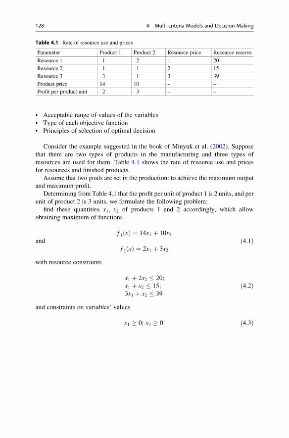
• Acceptable range of values of the variables
• Type of each objective function
• Principles of selection of optimal decision
Consider the example suggested in the book of Minyuk et al. (2002). Suppose
that there are two types of products in the manufacturing and three types of
resources are used for them. Table 4.1 shows the rate of resource use and prices
for resources and finished products.
Assume that two goals are set in the production: to achieve the maximum output
and maximum profit.
Determining from Table 4.1 that the profit per unit of product 1 is 2 units, and per
unit of product 2 is 3 units, we formulate the following problem:
find these quantities x1, x2 of products 1 and 2 accordingly, which allow
obtaining maximum of functions
f 1 xð Þ ¼ 14x1 þ 10x2and
f 2 xð Þ ¼ 2x1 þ 3x2
ð4:1Þ
with resource constraints
x1 þ 2x2 � 20;x1 þ x2 � 15;3x1 þ x2 � 39
ð4:2Þ
and constraints on variables’ values
x1 � 0; x2 � 0: ð4:3Þ
Table 4.1 Rate of resource use and prices
Parameter Product 1 Product 2 Resource price Resource reserve
Resource 1 1 2 1 20
Resource 2 1 1 2 15
Resource 3 3 1 3 39
Product price 14 10 – –
Profit per product unit 2 3 – –
128 4 Multi-criteria Models and Decision-Making
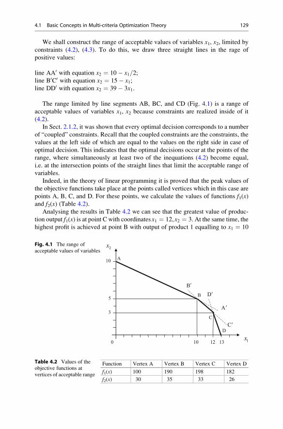
We shall construct the range of acceptable values of variables x1, x2, limited by
constraints (4.2), (4.3). To do this, we draw three straight lines in the rage of
positive values:
line AA0 with equation x2 ¼ 10� x1=2;line B0C0 with equation x2 ¼ 15� x1;line DD0 with equation x2 ¼ 39� 3x1.
The range limited by line segments AB, BC, and CD (Fig. 4.1) is a range of
acceptable values of variables x1, x2 because constraints are realized inside of it
(4.2).
In Sect. 2.1.2, it was shown that every optimal decision corresponds to a number
of “coupled” constraints. Recall that the coupled constraints are the constraints, the
values at the left side of which are equal to the values on the right side in case of
optimal decision. This indicates that the optimal decisions occur at the points of the
range, where simultaneously at least two of the inequations (4.2) become equal,
i.e. at the intersection points of the straight lines that limit the acceptable range of
variables.
Indeed, in the theory of linear programming it is proved that the peak values of
the objective functions take place at the points called vertices which in this case are
points A, B, C, and D. For these points, we calculate the values of functions f1(x)and f2(x) (Table 4.2).
Analysing the results in Table 4.2 we can see that the greatest value of produc-
tion output f1(x) is at point C with coordinatesx1 ¼ 12,x2 ¼ 3. At the same time, the
highest profit is achieved at point B with output of product 1 equalling to x1 ¼ 10
1x
2x
0 10 12 13
3
5
10A
B
C
D
A
C
B
D
Fig. 4.1 The range of
acceptable values of variables
Table 4.2 Values of the
objective functions at
vertices of acceptable range
Function Vertex A Vertex B Vertex C Vertex D
f1(x) 100 190 198 182
f2(x) 30 35 33 26
4.1 Basic Concepts in Multi-criteria Optimization Theory 129
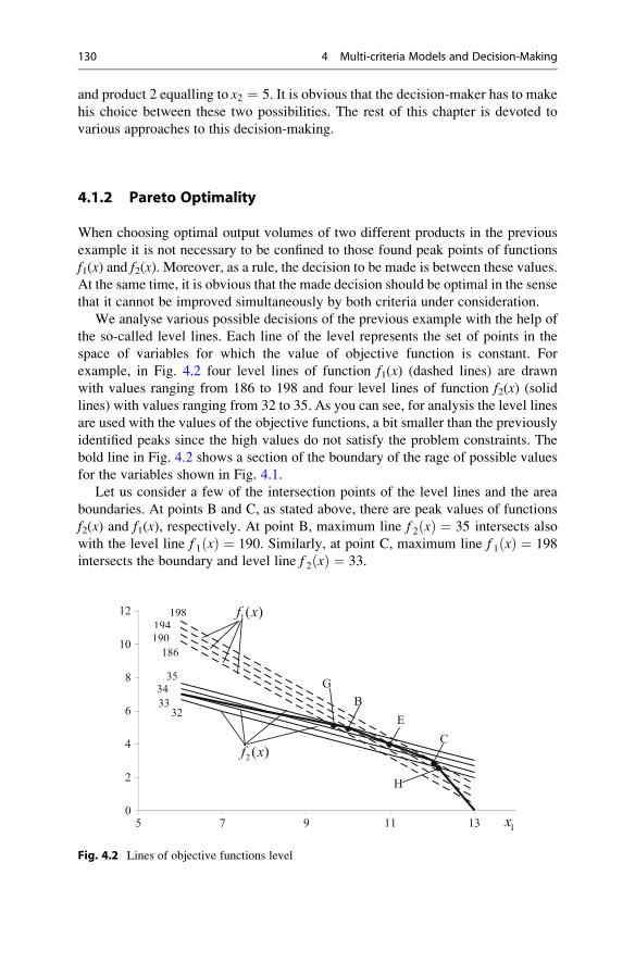
and product 2 equalling to x2 ¼ 5. It is obvious that the decision-maker has to make
his choice between these two possibilities. The rest of this chapter is devoted to
various approaches to this decision-making.
4.1.2 Pareto Optimality
When choosing optimal output volumes of two different products in the previous
example it is not necessary to be confined to those found peak points of functions
f1(x) and f2(x). Moreover, as a rule, the decision to be made is between these values.
At the same time, it is obvious that the made decision should be optimal in the sense
that it cannot be improved simultaneously by both criteria under consideration.
We analyse various possible decisions of the previous example with the help of
the so-called level lines. Each line of the level represents the set of points in the
space of variables for which the value of objective function is constant. For
example, in Fig. 4.2 four level lines of function f1(x) (dashed lines) are drawn
with values ranging from 186 to 198 and four level lines of function f2(x) (solidlines) with values ranging from 32 to 35. As you can see, for analysis the level lines
are used with the values of the objective functions, a bit smaller than the previously
identified peaks since the high values do not satisfy the problem constraints. The
bold line in Fig. 4.2 shows a section of the boundary of the rage of possible values
for the variables shown in Fig. 4.1.
Let us consider a few of the intersection points of the level lines and the area
boundaries. At points B and C, as stated above, there are peak values of functions
f2(x) and f1(x), respectively. At point B, maximum line f 2 xð Þ ¼ 35 intersects also
with the level line f 1 xð Þ ¼ 190. Similarly, at point C, maximum line f 1 xð Þ ¼ 198
intersects the boundary and level line f 2 xð Þ ¼ 33.
0
2
4
6
8
10
12
5 7 9 11 13
198194190
186
1( )f x
2( )f x
3233
3435
B
C
E
G
1x
H
Fig. 4.2 Lines of objective functions level
130 4 Multi-criteria Models and Decision-Making
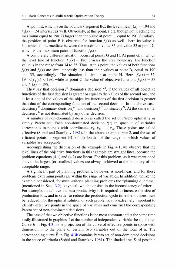
At point E, which is on the boundary segment BC, the level lines f 1 xð Þ ¼ 194and
f 2 xð Þ ¼ 34 intersect as well. Obviously, at this point, f1(x), though not reaching the
maximum equal to 198, is larger than the value at point C, equal to 190. Similarly,
the position of point E is observed for function f2(x) as well—here its value is
34, which is intermediate between the maximum value 35 and value 33 at point C,
which is the maximum point of function f1(x).A completely different situation occurs at points G and H. At point G, in which
the level line of function f 1 xð Þ ¼ 186 crosses the area boundary, the function
value is in the range from 34 to 35. Thus, at this point, the values of both functions
f1(x) and f2(x) are simultaneously less than their values at point B, equal to 190
and 35, accordingly. The situation is similar at point H. Here f 2 xð Þ ¼ 32,
194 < f 1 xð Þ < 198, while at point C the value of objective functions f 2 xð Þ ¼ 33
and f 1 xð Þ ¼ 198.
They say that decision f1 dominates decision f 2, if the values of all objective
functions of the first decision is greater or equal to the values of the second one, and
at least one of the values of the objective functions of the first decision is greater
than that of the corresponding function of the second decision. In the above case,
decision f B dominates decision f G and decision f C dominates f H. At the same time,
decision f E is not dominated by any other decision.
A number of non-dominated decision is called the set of Pareto optimality or
simply Pareto set. Each non-dominated decision f(x) in space m of variables
corresponds to point x with coordinates, x1, x2, . . ., xm. These points are called
effective (Sobol and Statnikov 1981). In the above example, m¼ 2, and the set of
efficient points is segment BC of the border of the range, in which values of
variables are acceptable.
Accomplishing the discussion of the example in Fig. 4.1, we observe that the
level lines of the objective functions in this example are straight lines, because the
problem equations (4.1) and (4.2) are linear. For this problem, as it was mentioned
above, the largest (or smallest) values are always achieved at the boundary of the
acceptable range.
A significant part of planning problems, however, is non-linear, and for these
problems extremum points are within the range of variables. In addition, unlike the
example considered, for multi-criteria planning problems the “planning dilemma”
(mentioned in Sect. 3.2) is typical, which consists in the inconsistency of criteria.
For example, to achieve the best productivity it is required to increase the size of
production lots, and in order to reduce the production cycle time the lot sizes must
be reduced. For the optimal solution of such problems, it is extremely important to
identify effective points in the space of variables and construct the corresponding
Pareto set of non-dominated decisions.
The case of the two objective functions is the most common and at the same time
easily illustrated in graphics. Let the number of independent variables be equal to n.Curve E in Fig. 4.3 is the projection of the curve of effective points in space with
dimension n to the plane of certain two variables out of the total of n. The
corresponding curve eE in Fig. 4.3b contains Pareto set of non-dominated decisions
in the space of criteria (Sobol and Statnikov 1981). The shaded area D of possible
4.1 Basic Concepts in Multi-criteria Optimization Theory 131
values on the plane of variables x1xn (Fig. 4.2a) is limited by certain values x1 and
xn, as well as the curve with a given criterion value f 2 ¼ f *2. We choose any point A0
on the set (curve) of efficient points. Each such point is at the same time the point of
contact of the level lines of criteria f1 and f2 passing through this point.
On the plane of criteria (Fig. 4.3b), area D goes into area eD, the curve E goes into
curve eE, and A0 point goes to point B0 with coordinates a and b. Area eD itself is an
area of acceptable but not enough effective decisions, and the boundary of this areaeE is a set of effective decisions.
Line eE is called a trade-off curve. All points of the trade-off curve represent
non-dominated decisions. At transition from one point to another point of this curve
the value of one of the criteria increases, and the value of another certainly
decreases. This kind of trade-off curve is typical for the case where it is desirable
to simultaneously increase or decrease both optimization criteria. If one of the
criteria must be increased, and another must be decreased, the trade-off curve also
exists but has a slightly different form, as will be shown below.
Unlike the trade-off curve, curve E can be of any nature and even become a
straight line. As the final decision, one of the points of trade-off curve should be
taken, the combination of the criteria values of which is the most acceptable from
the point of view of the decision-maker.
4.1.3 Main Methods of Solving Multi-criteria Planning Problems
Most of the methods for solving multi-objective problems belong to one of three
groups:
D
E0A
2f b=
1f a=
*2 2f f=
1x
nx
1f
2f
*2 2f f=
0B
2f b=
1f a=
D
E
а) b)
Fig. 4.3 Effective points in the space of variables and Pareto points in the space of criteria
132 4 Multi-criteria Models and Decision-Making
• Methods of theory of utility
• Methods based on criteria space metric
• Methods of hierarchal analysis
The methods of the first group were mentioned above in Sect. 1.7.3. Methods of
the first and second groups are used when all the relevant criteria have comparable
value. These will be considered further in the various chapters of this book. In cases
when some of the criteria are much more important than the others, it makes sense
to use the methods of hierarchical analysis. In this book, these methods are not
considered.
The process of setting a multi-objective problem consists mainly of three steps
(T’Kindt and Billaut 2005). The first of them determines a number of possible
solutions; the second step describes the criteria and variables (attributes) of the
problem; and the third stage defines the utility function of each criterion. In the
process of solving the problem the attribute values are searched, which maximize
the utility of criteria. In the theory of multi-criteria optimization, it is proved that the
optimal solution can be found almost always.
In solving the problems of planning the set of possible solutions usually consists
of a set of lots of different products that can be released for manufacturing in
specific time periods. Optimal solution should obviously consist in determination of
the lot sizes in each period, and for the development of such a decision, the quality
criteria must be set.
Above Tables 2.5–2.7 show exemplary sets of criteria for each of the basic types
of production. Section 2.2.3 gives the analysis of these tables, from which it follows
that the quality of a particular plan is mainly determined by the values of direct or
indirect costs and performance of various obligations. Such obligations may be not
only the need to fulfil orders, but also to maintain the size of reserves.
In the simplest cases, the criterion of order fulfilment is defined as makespan
Cmax or a minimum value of the maximum delay of orders fulfilment Tmax; at that
the first criterion is preferable for “to stock” strategy and the second “to order”
strategy. The criteria are calculated at the time of planning for a specific duration of
the plan implementation—for some planning horizon.
In order to achieve the calculated values of the criteria, there must be strict
adherence to the plan, which is difficult to perform, at least for “to order” strategy.
This situation is due, firstly, to the difficulty in determining the initial conditions of
the plan—time of readiness of processed products and equipment. Secondly, during
the time of the plan implementation new jobs can appear, the conditions of
equipment operation and personnel work can change, etc. Therefore, in practice,
at least at the level of operational plans, we have to use not only the optimization
planning using Tmax or Cmax, but rather the planning by the priority of jobs. In multi-
criteria planning, it is useful to use utility functions as criteria.
Instead of the criterion of direct costs (K1 in Tables 2.5–2.7) the function of
negative utility of costs (function of loss) can be introduced to perform n jobs on theplanning horizon
4.1 Basic Concepts in Multi-criteria Optimization Theory 133
U ¼ 1
c
Xni¼1
ci; ð4:4Þ
where ci is value of costs, e.g. the changeovers from one job to another,, and
c is the cost of one shift.If the quantity of the orders on the planning horizon h is equal to n, their total
current utility is equal to the sum of utilities of each since the orders are usually
independent. Then the total value of the current utility function of the orders
according to Eq. (2.32):
V ¼Xni¼1
Vi ¼ 1
G
Xni¼1
wipi �Xni¼1
Hi; ð4:5Þ
where, as above, wi is the priority coefficient of i-type job, pi is the processing time
of the i-th job, G is the average quantity of days in planned period, and Hi is the
production intensity of i-th order.
In contrast to the examples in Sect. 4.1.2, the utility of criteria U and V has a
different focus. In fact, when planning we should try to have costs valueU as low as
possible and current utility V, on the contrary, as high as possible. In this case, the
dilemma of planning leads to another kind of trade-off curve: when moving along
the points of the curve, both criteria simultaneously either increase or decrease
depending on the direction of motion.
Using Table 1.2 of production scale corresponding to the production types, and
Tables 2.5–2.7, which describe the hierarchy of costs criteria K1–K6 and timely
performance of obligation C1 and C2, you can set a definite connection between
functionsU and V (Mauergauz 2012). Figure 4.4 shows Pareto diagram of functions
U and V for master plan and Fig. 4.5 for the operational plan.
The curves in Figs. 4.4 and 4.5 are a set of Pareto points, showing the quality of
the specific formed plan as a combination of the values of the loss function due to
the costs and current utility function. On these curves, there are the points
corresponding to different production scales and strategies.
Figures 4.4 and 4.5 make it obvious that the smaller the scale of production and
lower the level of the plan hierarchy, the greater the effect of the current utility
function of obligations performance. In this case, its optimal value becomes higher;
while the acceptable value of the loss function of the cost also increases. From this
result, we can draw several conclusions which directly define the setting of multi-
criteria optimization problems of planning.
• In mass and large-serial production, where it is primarily important to reduce the
costs, decrease of order utility can be assumed and thus the point of decision on
the Pareto diagram is in the area of small values of function V and U. In these
cases, for the purpose of optimization it is advisable to use one objective
function that minimizes the amount of costs, and the need to fulfil obligations
134 4 Multi-criteria Models and Decision-Making

can be taken into account using some limitations. This applies to both the master
and operational plans.
• For operational plans in small-serial production it also makes sense to use one
objective function, but minimizing the losses because of non-fulfilment of
obligations. In this variant, the decision point is in the area of big values of
V and U.• When finding the decision point in the middle section of the curve it is not
possible any more to be limited to one optimization criterion, in general case. In
some cases, for example, during developing master plan for serial, small-serial,
and project productions, one objective function of costs can remain by including
fines derived from non-fulfilment of obligations into it. However, in developing
the plans of the lower level—material requirement and, in particular, operational
plans, the cost issues fade into insignificance. For example, economic criteria
can be considered only when determining the size of the production lots and the
lead time is determined on the basis of the minimum delay in the performance of
obligations.
Small-serial MTO
0
U
V
Mass
Large-serial
Serial
Small-serial MTS Individual
Fig. 4.4 UV diagram for
master plans
0 V
U
Large-serial MTS
Large-serial MTO
Serial MTS
Serial MTOSmall-serial MTO
Mass
Individual
Small-serial MTSFig. 4.5 UV diagram for
operational plans
4.1 Basic Concepts in Multi-criteria Optimization Theory 135
Yet, in some cases, for example, when planning operation of the machine for
cutting sheets (serial or small-serial production), it is impossible to be limited by
one criterion. The main criterion of the plan when fulfilling the orders of machine
shops, as seen in Table 2.5, is criterion C1 of timely provision of these shops with
blanks. In this case, however, the need to consider other criteria is clearly seen:
perhaps the less labour input of cutting and delivery of the sheets K1 and material
saving when cutting sheet K2.
4.1.4 Analytical Method of Constructing a Trade-Off Curve
As mentioned above it follows that to solve the multi-criteria problem, you must
first construct a trade-off curve and then select the point of the curve that fits the real
requirements of the problem in the best way. Let us consider the problem with two
criteria that need to be let to go to a minimum by the optimal choice of set of
independent variables xi. Suppose for definiteness, for example, the increase of
values of any of the parameters leads to decrease of value f1(x) and increase of valuef2(x).
In formulating the multi-criteria problem we can always assume that one of the
criteria serves as an objective function of the one-criterion problem, and the rest of
the criteria are constraints. Suppose that one of the criteria, for example, f2(x), is theobjective function and the second f1(x) is the constraint with the set value f 1 xð Þ ¼ a(Fig. 4.6).
Along the coordinate axes, similar to Fig. 4.3b, on Fig. 4.6 the criteria values are
plotted. At the point of X-axis with f 1 ¼ awe draw a vertical straight line, which is
the locus of all the states of the system with f 1 ¼ a. Let us consider a state of thesystem (point B1), characterized by a set of values (a, b1).
Now we will increase by one of the independent variables. For example, suppose
that if x1 change the system will transfer from state B1 to state L1, if x2 change—to
1f
2f
2 1f b=
2 2f b=
1f a=
2B
1L
2L
nL
1αnα
ε
1B
Fig. 4.6 Algorithm to
construct points of the trade-
off curve
136 4 Multi-criteria Models and Decision-Making
state L2, if xn change—to state Ln. Now by linking point B1 to new points Liwe get asheaf of vectors characterizing the transitions from the initial state to some other
one by varying the independent variables of the system. The larger the vector’s
angle of inclination towards the X-axis, the greater the decrease of f2(x) at
the same increases of f1(x). Therefore, out of the entire set of vectors, the “best”
effect on the system is produced by the vector with the greatest inclination to
the X-axis and the “worst” with the smallest inclination. In this case, this “best”
vector is B1Ln and the “worst” vector is B1L1.When moving from point B1 to Ln the value of f2(x) decreases, but the value of
criterion f1(x) increases, and thereby the accepted condition of constancy of limit
f 1 ¼ a is violated. To maintain the constant limit value it is obviously necessary to
go back to the state illustrated by the point on line f 1 ¼ a.This yields the idea that in order to “improve” the state of the system it is
advisable first to go from point B1 to point Ln, i.e. pass along the vector with the
largest angle of inclination αn, and then come back from point Ln to line f 1 ¼ aalong the vector with the smallest inclination α1. In this case, the state of the systemwill be clearly better than the initial, because limit f 1 ¼ a will be valid, and the
values of criterion f2(x) at obtained point B2 will be clearly smaller than the initial
one. This process can be continued until angle ε of the opening of vector sheaf
equals 0.
Given that the tangent of the inclination of each vector is represented by a
derivative from f2(x) by f1(x) at changing only one of the independent variables,
the equal-zero condition of angle opening ε will be as follows:
∂f 2 x1ð Þ∂f 1 x1ð Þ ¼
∂f 2 x2ð Þ∂f 1 x2ð Þ ¼ . . . ¼ ∂f 2 xnð Þ
∂f 1 xnð Þ : ð4:6Þ
The derivatives in expression (4.6) depend on the parameters. Using the differ-
entiation formula of the implicit function
df 2 xð Þdf 1 xð Þ ¼
df 2 xð Þdx
=df 1 xð Þdx
we obtain the equation system
∂f 2∂xi
� ∂f 1∂xk
¼ ∂f 2∂xk
� ∂f 1∂xi
, i ¼ 1 . . . n, k ¼ 1 . . . n, i 6¼ k: ð4:7Þ
The number of linearly independent equations (4.7) with any number of inde-
pendent variables is always one less than number n of independent variables xi. Sotheir solution gives not one specific optimal set of variables, but the set of these
values form a trade-off curve. Selection of the most appropriate point on the trade-
off remains with the decision-maker.
From the geometric point of view, equation (4.7) describes the curves lying in the
planes which at the same time touch surfaces f2(x1, x2, . . . xn) and f1(x1, x2, . . . xn).
4.1 Basic Concepts in Multi-criteria Optimization Theory 137
Therefore, the method is called the method of common tangents (Mauergauz 1999).
The example of use of equations (4.7) for the problems of planning is presented
below in Sect. 4.2.2.
4.2 Optimized Multi-criteria Lot Sizing
The scientific literature describes two methods of multi-criteria optimization of lot
sizes. In the first case, the solution of the optimization problem with one objective
function, which is a combination of several criteria, is searched. The second
approach is based directly on construction of the trade-off curve and the solution
is selected on this curve. We begin consideration of the first method.
4.2.1 Lot Sizing Based on Costs and Equipment
In the paper of Missbauer (2002), the optimization of lot sizing is based simulta-
neously on minimization of the cost of setup and storing similar to EOQ model,
described in Sect. 2.1.1, and minimization of the waiting time similar to the model
described in Sect. 3.4.1. At the same time, as usual, the constant demand for each
product Di is assumed. Every possible solution is represented by a set of values of
lots of each i-th product, characterized by the costs for setup and storage, as well asthe average waiting time of the lot for processing.
Workload of machine u consists of processing load of each i-th product lot
u ¼Xni¼1
ui ¼Xni¼1
Di
Pi;
where, the same as above, Pi is the machine capacity pcs/h.
To construct the trade-off curves “cost–waiting time” the following problem is
to be solved:
ð1� γÞXNi¼1
chiQi
2þ coiDi
Qi
!þ γwðQÞ, ð4:8Þ
with constraint
Xni¼1
Di=Pi þ Disi=Qið Þ < 1 ð4:9Þ
and at any (or at least several) values of weighing factor γ, which can be changed
from 0 to 1. Constraint (4.9) means that the average load coefficientK should be less
than one. In expressions (4.8) and (4.9) in analogy with Sects. 2.1.1 and 3.4.1 coi iscosts for i-th order fulfilment, chi is costs for storage of i-th product, Qi is the size of
138 4 Multi-criteria Models and Decision-Making
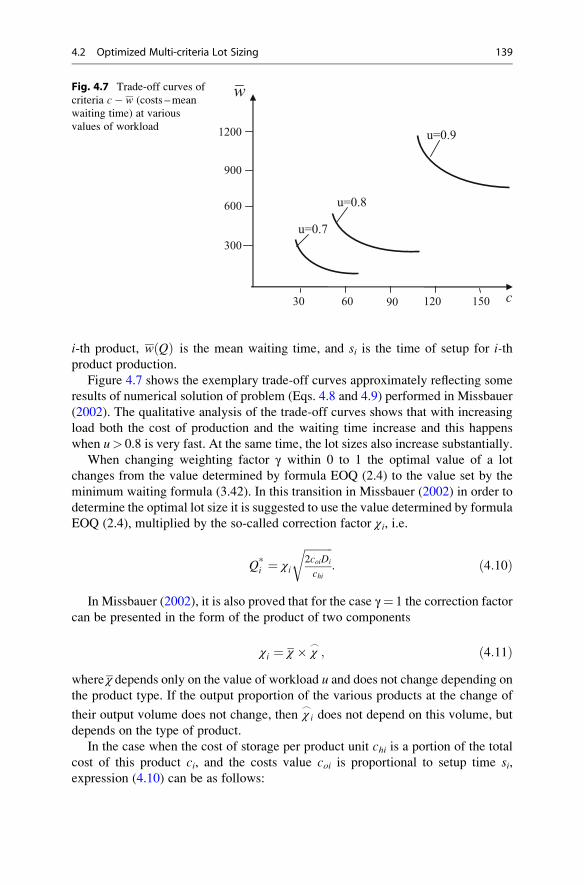
i-th product, w Qð Þ is the mean waiting time, and si is the time of setup for i-thproduct production.
Figure 4.7 shows the exemplary trade-off curves approximately reflecting some
results of numerical solution of problem (Eqs. 4.8 and 4.9) performed in Missbauer
(2002). The qualitative analysis of the trade-off curves shows that with increasing
load both the cost of production and the waiting time increase and this happens
when u> 0.8 is very fast. At the same time, the lot sizes also increase substantially.
When changing weighting factor γ within 0 to 1 the optimal value of a lot
changes from the value determined by formula EOQ (2.4) to the value set by the
minimum waiting formula (3.42). In this transition in Missbauer (2002) in order to
determine the optimal lot size it is suggested to use the value determined by formula
EOQ (2.4), multiplied by the so-called correction factor χi, i.e.
Q*i ¼ χi
ffiffiffiffiffiffiffiffiffiffi2coiDi
chi
r: ð4:10Þ
In Missbauer (2002), it is also proved that for the case γ¼ 1 the correction factor
can be presented in the form of the product of two components
χi ¼ χ � χ_; ð4:11Þ
where χ depends only on the value of workload u and does not change depending onthe product type. If the output proportion of the various products at the change of
their output volume does not change, then χ_i does not depend on this volume, but
depends on the type of product.
In the case when the cost of storage per product unit chi is a portion of the total
cost of this product ci, and the costs value coi is proportional to setup time si,expression (4.10) can be as follows:
c
w
30 60 90 120 150
300
600
900
1200
u=0.7
u=0.8
u=0.9
Fig. 4.7 Trade-off curves of
criteria c� w (costs –mean
waiting time) at various
values of workload
4.2 Optimized Multi-criteria Lot Sizing 139
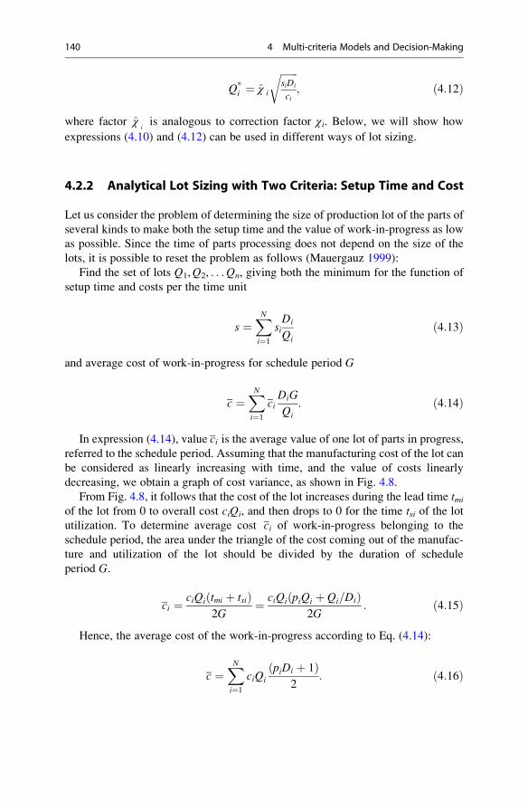
Q*i ¼ χ i
ffiffiffiffiffiffiffisiDi
ci
r; ð4:12Þ
where factor χiis analogous to correction factor χi. Below, we will show how
expressions (4.10) and (4.12) can be used in different ways of lot sizing.
4.2.2 Analytical Lot Sizing with Two Criteria: Setup Time and Cost
Let us consider the problem of determining the size of production lot of the parts of
several kinds to make both the setup time and the value of work-in-progress as low
as possible. Since the time of parts processing does not depend on the size of the
lots, it is possible to reset the problem as follows (Mauergauz 1999):
Find the set of lots Q1,Q2, . . .Qn, giving both the minimum for the function of
setup time and costs per the time unit
s ¼XNi¼1
siDi
Qi
ð4:13Þ
and average cost of work-in-progress for schedule period G
c ¼XNi¼1
ciDiG
Qi
: ð4:14Þ
In expression (4.14), value ci is the average value of one lot of parts in progress,referred to the schedule period. Assuming that the manufacturing cost of the lot can
be considered as linearly increasing with time, and the value of costs linearly
decreasing, we obtain a graph of cost variance, as shown in Fig. 4.8.
From Fig. 4.8, it follows that the cost of the lot increases during the lead time tmiof the lot from 0 to overall cost ciQi, and then drops to 0 for the time tsi of the lotutilization. To determine average cost ci of work-in-progress belonging to the
schedule period, the area under the triangle of the cost coming out of the manufac-
ture and utilization of the lot should be divided by the duration of schedule
period G.
ci ¼ ciQiðtmi þ tsiÞ2G
¼ ciQiðpiQi þ Qi=DiÞ2G
: ð4:15Þ
Hence, the average cost of the work-in-progress according to Eq. (4.14):
c ¼XNi¼1
ciQi
ðpiDi þ 1Þ2
: ð4:16Þ
140 4 Multi-criteria Models and Decision-Making
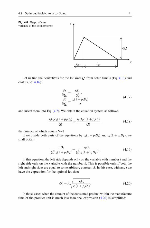
Let us find the derivatives for the lot sizes Qi from setup time s (Eq. 4.13) andcost c (Eq. 4.16):
∂s∂Qi
¼ � siDi
Q2i
,
∂c∂Qi
¼ ci 1þ piDið Þ2
ð4:17Þ
and insert them into Eq. (4.7). We obtain the equation system as follows:
siDick 1þ pkDkð ÞQ2
i
¼ skDkci 1þ piDið ÞQ2
k
; ð4:18Þ
the number of which equals N – 1.
If we divide both parts of the equations by ci 1þ piDið Þ and ck 1þ pkDkð Þ, weshall obtain:
siDi
Q2i ci 1þ piDið Þ ¼
skDk
Q2kck 1þ pkDkð Þ : ð4:19Þ
In this equation, the left side depends only on the variable with number i and theright side only on the variable with the number k. This is possible only if both the
left and right sides are equal to some arbitrary constant A. In this case, with any i wehave the expression for the optimal lot size:
Q*i ¼ A
ffiffiffiffiffiffiffiffiffiffiffiffiffiffiffiffiffiffiffiffiffiffiffiffisiDi
ci 1þ piDið Þ
s: ð4:20Þ
In those cases when the amount of the consumed product within the manufacture
time of the product unit is much less than one, expression (4.20) is simplified:
t
i ic Q
c
mit sit
Fig. 4.8 Graph of cost
variance of the lot in progress
4.2 Optimized Multi-criteria Lot Sizing 141

Q*i ¼ A
ffiffiffiffiffiffiffiffisiDi
ci
r: ð4:21Þ
Accordingly, expression (4.16) is simplified:
c ¼ 1
2
XNi¼1
ciQi: ð4:22Þ
By comparing Eqs. (4.12) and (4.21) we can see that constant A in formula (4.21)
coincides with the value of correction factor χ , and in this case this factor does not
depend on the type of product i. Let us consider the example of formula (4.21).
Suppose that a machine manufactures three products (Table 4.3).
By setting various values of correction factor Awe build the diagram of effective
points and level lines of criteria in the space of variables Qi (Fig. 4.9а) and the
trade-off curve for criteria s and c (Fig. 4.9b).Figure 4.9а shows projection E of the effective points line in the space of
variables to plane Q1Q2. The diagrams in Fig. 4.9 are similar to the relevant
diagrams in Fig. 4.3 with the difference that, in this case line E is straight, as in
accordance with Eq. (4.21)
Q*2 ¼ Q*
1
ffiffiffiffiffiffiffiffiffiffiffiffiffiffis2D2c1s1D1c2
r:
At each point of straight line E, for example, at point A0 with coordinates
Q1 ¼ 100 and Q2 ¼ 70, level lines s and c are tangents to each other, as shown
in Fig. 4.9а. Level lines c ¼ Const are the straight lines because according to
Eq. (4.16) c depends on the lot sizes Q1,Q2, . . .Qn linearly. Level lines s ¼ Const
have the form of hyperboles defined by relationship (4.13). Point A0 of line
E corresponds to point B0 on the trade-off curve eE with coordinates c ¼ 6300
and s ¼ 1:25 h.From the above Sects. (4.2.1) and (4.2.2), it follows that the mathematical
solution of the problem of multi-criteria optimization is to build a trade-off curve,
but this is not enough to obtain specific values of the optimal lots. In fact, the
mathematical solution allows the user choosing from a limited set of options that do
not dominate each other. The result is that the decision-maker must make a final
choice on some additional grounds. The methods of this choice are discussed below
in this chapter.
Table 4.3 Products manufactured on the machine
Product no. Setup time si, h Demand Di, pcs/day Product cost ci, $/pcs
1 2 40 80
2 1 10 20
3 1 20 50
142 4 Multi-criteria Models and Decision-Making
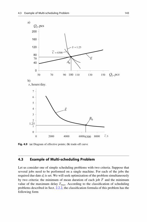
4.3 Example of Multi-scheduling Problem
Let us consider one of simple scheduling problems with two criteria. Suppose that
several jobs need to be performed on a single machine. For each of the jobs the
required due date di is set. We will seek optimization of the problem simultaneously
by two criteria: the minimum of mean duration of each job F and the minimum
value of the maximum delay Tmax. According to the classification of scheduling
problems described in Sect. 2.2.2, the classification formula of this problem has the
following form
0
40
80
120
160
200
50 70 90 110 130 150
а)
0
1
2
3
4
5
6
7
0 2000 4000 6000 8000
b)
1.25
0A
6300C =
1.25S =
1,Q pcs
2,pcsQ
E70
100
0B
, $С
, hours/day.s
6300
E
Fig. 4.9 (a) Diagram of effective points; (b) trade-off curve
4.3 Example of Multi-scheduling Problem 143
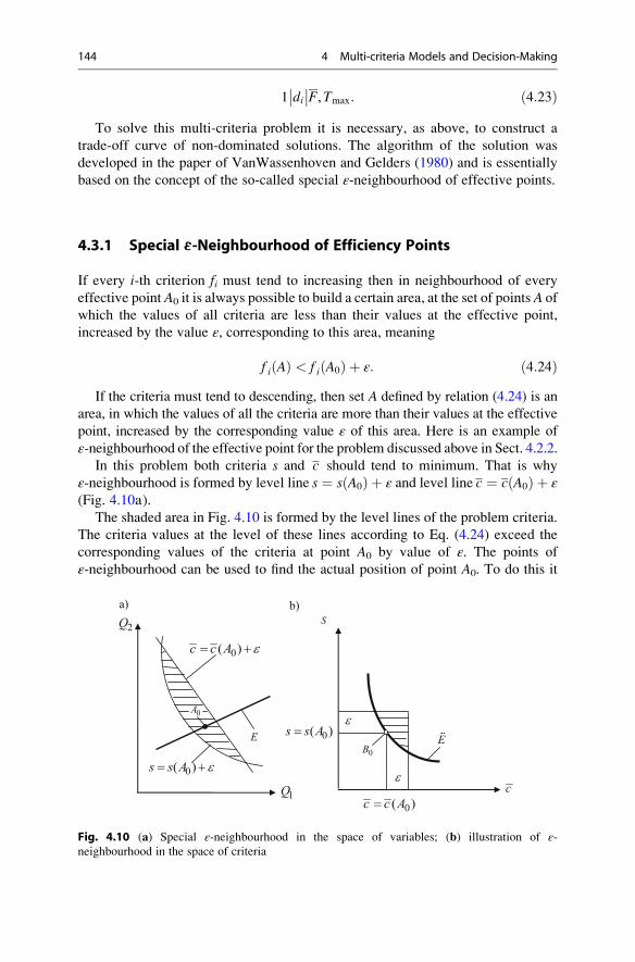
1��di��F,Tmax: ð4:23Þ
To solve this multi-criteria problem it is necessary, as above, to construct a
trade-off curve of non-dominated solutions. The algorithm of the solution was
developed in the paper of VanWassenhoven and Gelders (1980) and is essentially
based on the concept of the so-called special ε-neighbourhood of effective points.
4.3.1 Special e-Neighbourhood of Efficiency Points
If every i-th criterion fi must tend to increasing then in neighbourhood of every
effective point A0 it is always possible to build a certain area, at the set of points A of
which the values of all criteria are less than their values at the effective point,
increased by the value ε, corresponding to this area, meaning
f i Að Þ < f i A0ð Þ þ ε: ð4:24ÞIf the criteria must tend to descending, then set A defined by relation (4.24) is an
area, in which the values of all the criteria are more than their values at the effective
point, increased by the corresponding value ε of this area. Here is an example of
ε-neighbourhood of the effective point for the problem discussed above in Sect. 4.2.2.
In this problem both criteria s and c should tend to minimum. That is why
ε-neighbourhood is formed by level line s ¼ sðA0Þ þ ε and level line c ¼ cðA0Þ þ ε(Fig. 4.10а).
The shaded area in Fig. 4.10 is formed by the level lines of the problem criteria.
The criteria values at the level of these lines according to Eq. (4.24) exceed the
corresponding values of the criteria at point A0 by value of ε. The points of
ε-neighbourhood can be used to find the actual position of point A0. To do this it
Fig. 4.10 (a) Special ε-neighbourhood in the space of variables; (b) illustration of ε-neighbourhood in the space of criteria
144 4 Multi-criteria Models and Decision-Making

is obvious that one has to set the initial point of ε-neighbourhood and then using therelevant algorithm to decrease value ε gradually, pulling the shaded area to the
point.
Figure 4.10b shows that special ε-neighbourhood of effective point A0 in the
space of criteria meets the one-sided pyramid (shaded) neighbourhood of Pareto
point B0.
4.3.2 Solving Algorithm
We continue to solve the problem set above in this section by the specific example.
Suppose that in the beginning of the month, using the minimum criterion of mean
duration of each job F and the minimum value of the maximum tardiness Tmax it is
required to schedule jobs for a single machine, the data of which is given in
Table 4.4.
The idea of the described algorithm is based on theorems 1 and 2 from Sect.
2.3.2. Recall that theorem 1 states that the smallest mean duration of the production
cycle F is achieved by using the rules of the smallest processing time SPT.
Accordingly, theorem 2 states that the minimum value for the maximum deviation
of i-th job from the set due date Lmax (as well as for the tardiness Tmax) is achieved
by using the EDD rules, in which the priority is given to the job with the nearest
contractual due date di.In accordance with these theorems the described algorithm uses the combined
priority rule SPT/EDD, and criterion Tmax is used as a gradually decreasing
constraint of the form
Tmax � ε; ð4:25Þand criterion F is used as the objective function. Constraint (4.25) means that the
maximum possible due dates must be within this neighbourhood, i.e.
d ¼ di þ ε: ð4:26ÞTo use SPT rule the data in Table 4.4 is sorted in ascending order of processing
time. Figure 4.11 shows the block diagram of the algorithm. At the beginning of the
algorithm the initial values of the external cycle are set, which include the value of
Table 4.4 Data on the
planned jobsJob no. Processing time pi, work. days Due date di
1 2 24
2 4 22
3 5 18
4 7 23
5 10 21
4.3 Example of Multi-scheduling Problem 145

ε-neighbourhood of the due date in this neighbourhood. As the initial value of ε it isadvisable to take the full processing time of all the jobs, i.e.
ε1 ¼XNi¼1
pi: ð4:27Þ
In the process of work, two nested cycles are performed: external and internal.
Possible specific schedule is drawn up during operation of the internal cycle. The
work of the outer cycle is to change value ε, which prepares the new job of the inner
cycle. At each subsequent step k+ 1 new value ε-neighbourhood is defined as
4. Internal cycle continuesuntil condition2 is fulfilled
2. External cycle continuesuntil condition 1is fulfilled
Beginning
1.Initial values of
external cycle
3.Initial values of
internal cycle
6.Is condition 2fulfilled?
12. Change of initial values of external loop
10. Is condition 1 fulfilled?
End
7. Filling of set Sof schedule from set F under
condition 4
9. Change of initial values of internal loop
5. Selection of datafrom set L to intermediate set Fby condition 3
Yes
No
No
Yes
11.Consolidation of schedules into set E of effective points
8. Exclusion of the selected in block 7 jobs from set L
Internal cycle
continues
External cyclecontinues
Fig. 4.11 Block diagram of scheduling algorithm
146 4 Multi-criteria Models and Decision-Making
εkþ1 ¼ Tmax,k � 1: ð4:28ÞCriteria values for each of the schedules constructed thereby represent a single
point of the trade-off curve.
In this algorithm operation several different sets are used. All planned jobs in
accordance with Table 4.4 constitute set T, sorted in ascending order of processing
time pi. Additional set L at the beginning of each inner cycle (block 3) is equal to
set T, and then sequentially it excludes the jobs satisfying condition 3, which are
placed in set F (block 5). From the set F the jobs are selected in the order determined
by condition 4, which creates a new schedule in set S (block 7). Schedules
generated this way are accumulated in set E (block 11).
As you can see from Fig. 4.11, the algorithm uses two conditions of cycle
operation and two conditions of selection of set members.
Condition 1 is that the outer cycle operates by the flag value which is set in the
internal cycle: if the flag Q¼ 0 the outer cycle operates; if Q¼ 1 the operation
stops. Setting the flag to value of Q¼ 1 is defined by the absence of members in
set F.
Condition 2 is determined by the value of the same flag Q, and the presence of
members in set L as well: internal cycle operates, if Q¼ 0 andL 6¼ 0; in violation of
these conditions the cycle stops.
Condition 3 determines the selection from set L to set F of job Ji with number i,for which
d i �XJk ∈L
pk: ð4:29Þ
Condition 4 establishes the selection of such element as Ji out of set F for
schedule S, for which
pi ¼ maxJk ∈ F
pkð Þ: ð4:30Þ
Let us consider the algorithm operation by the example of the data in Table 4.4.
Step 1. The initial values of external cycle (block 1) are defined according to
formulas (4.26) and (4.27):
ε1 ¼XNi¼1
pi ¼ 28; d 1 ¼ d1 þ ε1 ¼ 52; d 2 ¼ 50; d 3 ¼ 46; d 4 ¼ 51; d 5
¼ 49:
Besides, flag Q¼ 0 and output set E¼ 0 are defined.
Step 2. Start of the external cycle.
2.1. Setting the values of the internal cycle (block 3):
Set L ¼ J1; J2; J3; J4; J5f g; the set of first schedule S1 ¼ 0.
Step 2.2. Start of the internal cycle.
4.3 Example of Multi-scheduling Problem 147
2.2.1. Calculation of the value
u ¼XJk ∈L
pk ¼ 28:
2.2.2. Selection (block 5) of members L to F under condition (4.29). Since all d i are
defined on Step 0, F ¼ J1; J2; J3; J4; J5f g meet this condition.
2.2.3. Finding the job with the highest processing time under condition (4.30): i¼ 5.
2.2.4. Transfer of job J5 (block 7) to set S: S1 ¼ J5f g.2.2.5. Exclusion of job J5 from set L (block 8): L ¼ J1; J2; J3; J4f g.Step 2.3. Continuation of internal cycle
u ¼XJk ∈L
pk ¼ 18; F ¼ J1, J2, J3, J4f g; i ¼ 4; S1 ¼ J4; J5f g; L ¼ J1; J2; J3f g:
When filling the set S, which is the possible schedule, the new members are inserted
in front of the existing ones.
Step 2.4. Continuation of internal cycle
u ¼ 11; F ¼ J1; J2; J3f g; i ¼ 3; S1 J3; J4; J5f g; L ¼ J1; J2f g:Step 2.5.
u ¼ 6; F ¼ J1; J2f g; i ¼ 2; S1 J2; J3; J4; J5f g; L ¼ J1f g:Step 2.6.
u ¼ 2; F ¼ J1f g; i ¼ 1; S1 J1; J2; J3; J4; J5f g; L ¼ 0:
Step 2.7. End of internal cycle
2.7.1. As L¼ 0, then under condition 2 (block 6) the internal cycle stops. Since the
flag of end of external cycle is equal to Q¼ 0, the external cycle continues (block
11) and the first possible schedule is transferred to the set of effective points
E ¼ S1 ¼ J1; J2; J3; J4; J5f g.2.7.2. The criteria values at Pareto point, corresponding to schedule S1, are defined:
F ¼ F J1ð Þ þ F J2ð Þ þ F J3ð Þ þ F J4ð Þ þ F J5ð ÞN
¼ 2þ 6þ 11þ 18þ 28
5
¼ 13days:
and
Tmax ¼ max max 0; Ci � dið Þð Þ ¼ max�max 0; 2� 24ð Þ, max 0; 6� 22ð Þ,
max 0; 11� 18ð Þ, max 0; 18� 23ð Þ; max 0; 28� 21ð Þ ¼ 7 days.
2.7.3. The initial values of the external cycle are changed (block 12):
ε2 ¼ Tmax � 1 ¼ 7� 1 ¼ 6; d 1 ¼ d1 þ ε2 ¼ 30; d 2 ¼ 28; d 3 ¼ 24; d 4
¼ 29; d 5 ¼ 27:
Step 3. Continuation of the external cycle
3.1. Setting the values of the internal cycle (block 3):
Set L ¼ J1; J2; J3; J4; J5f g; the set of the second schedule S2 ¼ 0.
148 4 Multi-criteria Models and Decision-Making
3.2. Start of the internal cycle
u¼ 28; when selecting (block 5) members L to F for the jobs with numbers 3 and
5, condition (4.29) is not fulfilled and so F ¼ J1; J2; J4f g; i ¼ 4; S2 J4f g;L ¼ J1; J2; J3; J5f g.3.3. Continuation of the internal cycle
u ¼ 21; F ¼ J1; J2; J3; J5f g; i ¼ 5; S2 J5; J4f g; L ¼ J1; J2; J3f g:3.4. u¼ 11; F¼{J1, J2, J3}; i¼ 3; S2¼ {J3, J5, J4}; L¼{J1, J2}.3.5. u ¼ 6; F ¼ J1; J2f g; i ¼ 2; S2 J2; J3; J5; J4f g; L ¼ J1f g:3.6. u ¼ 2; F ¼ J1f g; i ¼ 1; S2 J1; J2; J3; J5; J4f g; L ¼ 0.
3.7. End of the internal cycle
E ¼ S1 þ S2 ¼ J1; J2; J3; J4; J5ð Þ; J1; J2; J3; J5; J4ð Þf g;
F ¼ F J1ð Þ þ F J2ð Þ þ F J3ð Þ þ F J5ð Þ þ F J4ð ÞN
¼ 2þ 6þ 11þ 21þ 28
5
¼ 13:6 days;
Tmax ¼ max�max 0; 2� 24ð Þ, max 0; 6� 22ð Þ, max 0; 11� 18ð Þ,
max 0; 28� 23ð Þ; max 0; 20� 21ð Þ ¼ 5 days;ε3 ¼ 5� 1 ¼ 4; d 1 ¼ d1 þ ε3 ¼ 28; d 2 ¼ 26; d 3 ¼ 22; d 4 ¼ 27; d 5
¼ 25:
Step 4. Continuation of the external cycle:
4.1. Set L ¼ J1; J2; J3; J4; J5f g; the set of the third schedule S2 ¼ 0.
4.2. Start of the internal cycle:
u¼ 28; when selecting (block 5) members L to F for the jobs with numbers
2, 3, 4, and 5, condition (4.29) is not fulfilled and so F ¼ J1f g; i ¼ 1;S3 J1f g; L ¼ J2; J3; J4; J5f g.4.3. Continuation of the internal cycle:
u ¼ 26; F ¼ J2; J4f g; i ¼ 4; S3 J4; J1f g; L ¼ J2; J3; J5f g:4.4 u ¼ 19; F ¼ J2; J3; J5f g; i ¼ 5; S3 J5; J4; J1f g; L ¼ J2; J3f g:4.5 u ¼ 19; F ¼ J2; J3f g; i ¼ 3; S3 J3; J5; J4; J1f g; L ¼ J2f g:4.6 u ¼ 4; F ¼ J2f g; i ¼ 2; S3 J2; J3; J5; J4; J1f g; L ¼ 0:4.7. End of the internal cycle:
E ¼ S1 þ S2 þ S3¼ J1; J2; J3; J4; J5ð Þ; J1; J2; J3; J5; J4ð Þ; J2; J3; J5; J4; J1ð Þf g;
F ¼ F J2ð Þ þ F J3ð Þ þ F J5ð Þ þ F J4ð Þ þ F J1ð ÞN
¼ 4þ 9þ 19þ 26þ 28
5
¼ 17:2 days;
Tmax ¼ max�max 0; 28� 24ð Þ, max 0; 4� 22ð Þ, max 0; 9� 18ð Þ,
max 0; 26� 23ð Þ; max 0; 18� 21ð Þ ¼ 4 days.
4.3 Example of Multi-scheduling Problem 149

ε4 ¼ 4� 1 ¼ 3; d 1 ¼ d1 þ ε4 ¼ 27; d 2 ¼ 25; d 3 ¼ 21; d 4 ¼ 26; d 5
¼ 24:
Step 5. End of the external cycle:
u¼ 28; when selecting (block 5) members L to F for all jobs, condition (4.29) is not
fulfilled, F¼ 0 and so flag Q¼ 1 is set.
As a result of the algorithmoperation three different scheduleswith non-dominated
and valuesF and Tmax are determined. Figure 4.12 shows the trade-off curve based on
these values. In T’Kindt and Billaut (2005) it is stated that the computational
experiments for this problem with the number of scheduled jobs equal to 50 give up
to 29 Pareto points.
4.4 Methods of Decision-Making Theory in Planning Problems
In the problems described in the previous sections of this chapter, it was shown that
the result of multi-criteria optimization is building of trade-off curves. However,
the known nature of a trade-off curve is insufficient for full solution of these
problems, because this curve consists of a number of non-dominated points.
Therefore, a trade-off curve is only the basis for decision making, which is done
by the planner himself.
4.4.1 Some Information from the Decision Making Theory
The whole set of managerial decisions to be made is divided into two large groups:
strictly conditioned and proactive. The former are usually related to the so-called
standard decision defined by the regulations and orders. Proactive decisions are the
choice of alternative behaviours of several possible, each of which entails a number
10
12
14
16
18
3 4 5 6 7 maxT
FFig. 4.12 Trade-off curve
for variants of schedules
150 4 Multi-criteria Models and Decision-Making
of positive and negative consequences. In this book, we consider only these
decisions.
The decision format will be mostly influenced by the kind of the problem
situation. According to the paper of Simon (1959) all the problems can be divided
into three classes.
• Well-structured problems are problems, in which the significant relations
between parameters may be expressed in a formal way.
• Ill-structured or mixed problems have both qualitative and quantitative
elements, and the qualitative, obscure, and uncertain aspects of the problems
tend to dominate.
• Unstructured or qualitatively expressed problems contain only the description of
the most important resources, attributes and characteristics, the quantitative
relationships of which are completely unknown.
The production planning problems are mainly well structured and allow
a numerical solution. However, when developing plans for quite long-term
prospects the planner faces uncertainty, especially in the assessment of marketing
opportunities. In these cases, the problems of planning may be ill-structured.
In addition to classification according to the degree of structuring, the problems,
on which it is necessary to make decisions, are characterized by three main
parameters. If decisions are made by one person, then the problem is of type J. If
the decision involves several persons, the problem relates to type G. If there are
several criteria the problem is considered to be of type A. Otherwise, the special
designation is not used, and it is assumed by default that there is only one criterion.
Similarly, if the problem is quite determined, the special type designation is not
provided. If the task is probabilistic, the designation of its type includes parameter
S. In this chapter, we consider well-structured problems such as JA, i.e. problems
with several criteria, on which the decisions are made by one person.
In the decision-making process several stages can be identified.
• Identification of possible decision area is needed to refer planning decision either
to organizational or to the technical or economic areas of activity.
• Determination of the decision type: the standard decision, the usual decision
with some modifications, the original decision.
• Description of the possible set of decisions and the limits of their values. The
range of possible decisions in the decision theory is called alternatives.
Alternatives can be independent and dependent. Independent ones are those
alternatives, any actions with which do not affect the quality of the other
alternatives. In this book, we consider only such alternatives.
• Analysis of the advantages and disadvantages of possible alternative.
• Assessment of the probability of each alternative.
• Comparison of decisions according to various criteria.
4.4 Methods of Decision-Making Theory in Planning Problems 151

The planning decision is usually the organizational decision, and its type, as a
rule, has a fairly standard nature with modifications, which depend on the current
production situation. As it was mentioned above in Sect. 4.1.3, in this book we use
methods for solving multi-criteria problems based on utility theory and the study of
criteria space metric.
For making planning decisions using the theory of utility, first of all, the
background information should be described, which is a set of possible alternatives
and the utility level of each of them. Such information can be convenient to be
represented in the form of the matrix, which for problems of JA type is as shown in
Table 4.5.
The data in Table 4.5 contain the set of possible variants Yi. For all the variants,utility values uij must be defined on each of the criteria fj. Simultaneously the
priorities (weights) values of each of criteria wj can be set.
One of the most common methods using the criteria space metric is the so-called
method of the shifted ideal in feature space. In this method, first the so-called ideal
object is formed. As a rule, this object does not really exist but embodies all the best
possible properties of different actually existing alternatives. The presence of such
an object sets the reference point when comparing real alternatives to the ideal
hypothetical option. In this case, the objects of the set of acceptable alternatives Yiare compared with the ideal object by the criterion of distance from the real object
to the ideal one. To calculate the distances the initial information should be
presented as shown in Table 4.6.
To compare the diverse criteria it is necessary to transfer to their normalized
non-dimensional values. Normalized values in the i-th alternative for each j-thcriterion for the criteria, during increasing of which the quality of the alternative
improves, are determined using the conversion
aij ¼fþj � f ij
� �fþj � f�j� � ; ð4:31Þ
where fþj is the value of j-th criterion of the ideal object and f�j is the value for j-th
criterion for the object being the worst by this criterion.
The distance between the objects can be set in different ways. In most cases we
use the generalized metric of the form
Table 4.5 Matrix of the
criteria utility description
for problems of JA type
Criteria (goals) f1 f2 . . . fkDecision alternatives
Y1 u11 u12 . . . u1kY2 u21 u22 . . . u2k. . . . . . . . . . . . . . .
Yn un1 un2 . . . unkGoal priorities w1 w2 . . . wk
152 4 Multi-criteria Models and Decision-Making
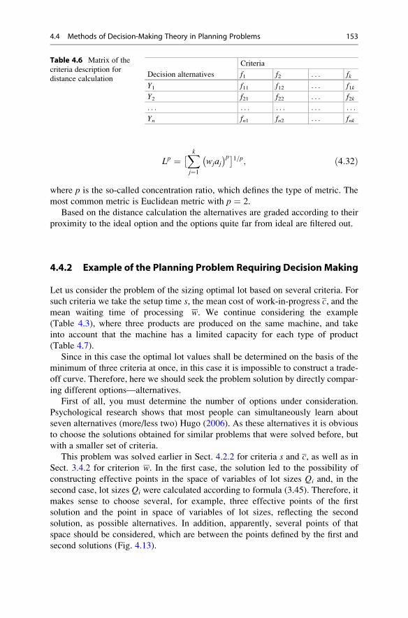
Lp ¼ �Xkj¼1
wjaj� p 1=p; ð4:32Þ
where p is the so-called concentration ratio, which defines the type of metric. The
most common metric is Euclidean metric with p ¼ 2.
Based on the distance calculation the alternatives are graded according to their
proximity to the ideal option and the options quite far from ideal are filtered out.
4.4.2 Example of the Planning Problem Requiring Decision Making
Let us consider the problem of the sizing optimal lot based on several criteria. For
such criteria we take the setup time s, the mean cost of work-in-progress c, and the
mean waiting time of processing w. We continue considering the example
(Table 4.3), where three products are produced on the same machine, and take
into account that the machine has a limited capacity for each type of product
(Table 4.7).
Since in this case the optimal lot values shall be determined on the basis of the
minimum of three criteria at once, in this case it is impossible to construct a trade-
off curve. Therefore, here we should seek the problem solution by directly compar-
ing different options—alternatives.
First of all, you must determine the number of options under consideration.
Psychological research shows that most people can simultaneously learn about
seven alternatives (more/less two) Hugo (2006). As these alternatives it is obvious
to choose the solutions obtained for similar problems that were solved before, but
with a smaller set of criteria.
This problem was solved earlier in Sect. 4.2.2 for criteria s and c, as well as inSect. 3.4.2 for criterion w. In the first case, the solution led to the possibility of
constructing effective points in the space of variables of lot sizes Qi and, in the
second case, lot sizes Qi were calculated according to formula (3.45). Therefore, it
makes sense to choose several, for example, three effective points of the first
solution and the point in space of variables of lot sizes, reflecting the second
solution, as possible alternatives. In addition, apparently, several points of that
space should be considered, which are between the points defined by the first and
second solutions (Fig. 4.13).
Table 4.6 Matrix of the
criteria description for
distance calculationDecision alternatives
Criteria
f1 f2 . . . fk
Y1 f11 f12 . . . f1kY2 f21 f22 . . . f2k. . . . . . . . . . . . . . .
Yn fn1 fn2 . . . fnk
4.4 Methods of Decision-Making Theory in Planning Problems 153

Points 1, 2, and 3 in Fig. 4.13 are projections to plane Q1Q2 of effective points,
defined for three different values of correction factor χ in formula (4.21): 50, 100,
and 150. For example, at point 1 χ ¼ χ 1 ¼ 50 and the lot of product 2 found by
formula (4.21).
Q21 ¼ χ 1
ffiffiffiffiffiffiffiffiffiffis2D2
C2
r¼ 50�
ffiffiffiffiffiffiffiffiffiffiffiffiffiffi1� 10
20
r¼ 35 pcs:
Point 4 displays the projection of the point in the space of variables, calculated
by formula (3.45). For example, with working day duration G ¼ 8 h.
Q24 ¼2P2
G�1�
X3j¼1
Dj
Pj
ffiffiffiffiffiffiffiffiffiffiffiffiffiffiffiffiffiffiffiffis2X3j¼1
sjDj
Pj
vuut ¼ 39pcs:
Now we increase the number of possible alternatives to a reasonable value in the
range of 5–9. Points 1, 2, and 3, located on the bold straight line, are solutions of the
problem of the optimal lot size, which was set out in Sect. 4.2.2, while point 4 is also
a solution of the problem of the optimal lot size given in Sect. 3.4.1. Apparently, it
Table 4.7 Products manufactured on the machine
Product
no.
Setup time
si, hDemand Di,
pcs/day
Product cost ci,$/pcs
Machine capacity Pi,
pcs/day
1 2 40 80 150
2 1 10 20 60
3 1 20 50 100
0
20
40
60
80
100
120
0 25 50 75 100 125 150 1Q
2Q
2
1
45
6
7
3
Fig. 4.13 Projection of the possible alternatives of solution to plane Q1Q2
154 4 Multi-criteria Models and Decision-Making
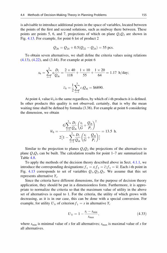
is advisable to introduce additional points in the space of variables, located between
the points of the first and second solutions, such as midway there between. These
points are points 5, 6, and 7, projections of which on plane Q1Q2 are shown in
Fig. 4.13. For example, for point 6 lot of product 2
Q26 ¼ Q24 þ 0:5ðQ22 � Q24Þ ¼ 55 pcs:
To obtain seven alternatives, we shall define the criteria values using relations
(4.13), (4.22), and (3.44). For example at point 6
s6 ¼X3i¼1
siDi
Qi6
¼ 2� 40
118þ 1� 10
55þ 1� 20
64¼ 1:17 h=day;
c6 ¼ 1
2
X3i¼1
ciQi6 ¼ $6890:
At point 4, valuew4 is the same regardless, by which of i-th products it is defined.In other products this quality is not observed; certainly, that is why the mean
waiting time shall be defined by formula (3.38). For example at point 6 considering
the dimension, we obtain
w6 ¼GX3i¼1
Di
Qi6
siGþ Qi6
Pi
� �2
2�1�
X3i¼1
Di
Qi6
siGþ Qi6
Pi
� � ¼ 13:5 h:
Similar to the projection to planes Q1Q2 the projections of the alternatives to
plane Q1Q3 can be built. The calculation results for point 1–7 are summarized in
Table 4.8.
To apply the methods of the decision theory described above in Sect. 4.1.1, we
introduce the corresponding designations: f 1 ¼ s; f 2 ¼ c; f 3 ¼ w. Each i-th point inFig. 4.13 corresponds to set of variables Q1,Q2,Q3. We assume that this set
represents alternative Yi.Since the criteria have different dimensions, for the purpose of decision theory
application, they should be put in a dimensionless form. Furthermore, it is appro-
priate to normalize the criteria so that the maximum value of utility in the above
set of alternatives is equal to 1. For the criteria, the utility of which grows with
decreasing, as it is in our case, this can be done with a special conversion. For
example, for utility U1i of criterion f 1 ¼ s in alternative Yi
U1i ¼ 1� si � smin
smax
; ð4:33Þ
where smin is minimal value of s for all alternatives; smax is maximal value of s forall alternatives.
4.4 Methods of Decision-Making Theory in Planning Problems 155
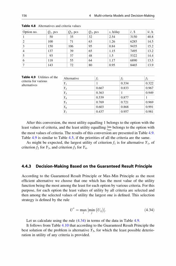
After this conversion, the most utility equalling 1 belongs to the option with the
least values of criteria, and the least utility equalling smin
smaxbelongs to the option with
the most values of criteria. The results of this conversion are presented in Table 4.9.
Table 4.9 is similar to Table 4.5, if the priorities of all the criteria are the same.
As might be expected, the largest utility of criterion f1 is for alternative Y1, ofcriterion f2 for Y3, and criterion f3 for Y4.
4.4.3 Decision-Making Based on the Guaranteed Result Principle
According to the Guaranteed Result Principle or Max-Min Principle as the most
efficient alternative we choose that one which has the most value of the utility
function being the most among the least for each option by various criteria. For this
purpose, for each option the least values of utility by all criteria are selected and
then among the selected values of utility the largest one is defined. This selection
strategy is defined by the rule
U* ¼ maxi
½minj
Uij
� �: ð4:34Þ
Let us calculate using the rule (4.34) in terms of the data in Table 4.9.
It follows from Table 4.10 that according to the Guaranteed Result Principle the
best solution of the problem is alternative Y5, for which the least possible deterio-
ration in utility of any criteria is provided.
Table 4.8 Alternatives and criteria values
Option no. Q1, pcs Q2, pcs Q3, pcs s, h/day c, $ w, h
1 50 35 32 2.54 3150 40.8
2 100 71 63 1.26 6285 14.5
3 150 106 95 0.84 9435 15.2
4 137 39 65 1.15 7495 13.2
5 93 37 48 1.5 5322 14.4
6 118 55 64 1.17 6890 13.5
7 143 72 80 0.95 8465 13.9
Table 4.9 Utilities of the
criteria for various
alternatives
Alternative f1 f2 f3
Y1 1 0.334 0.322
Y2 0.667 0.833 0.967
Y3 0.363 1 0.949
Y4 0.539 0.877 1
Y5 0.769 0.721 0.969
Y6 0.603 0.868 0.991
Y7 0.437 0.957 0.981
156 4 Multi-criteria Models and Decision-Making
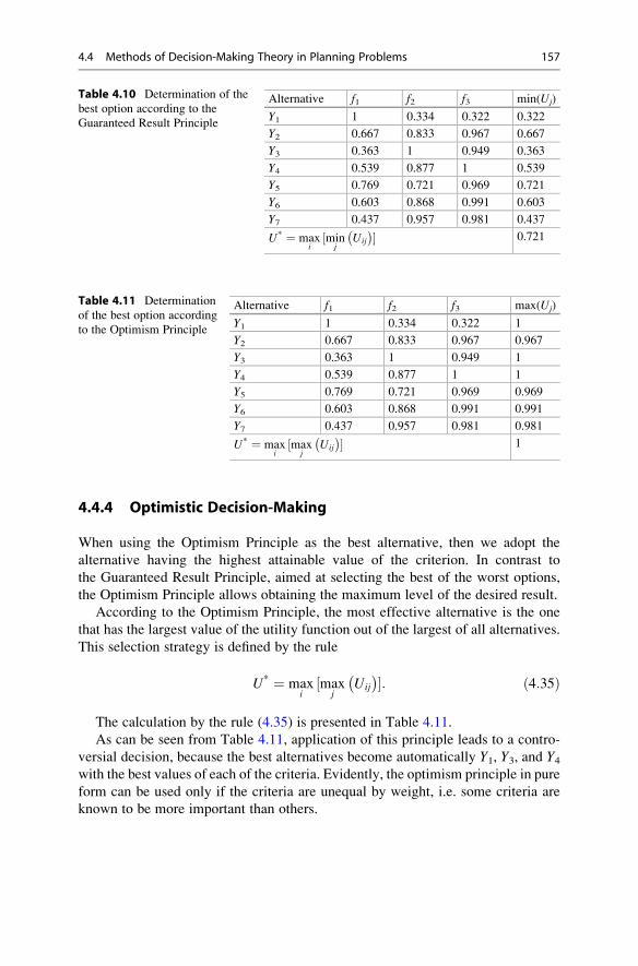
4.4.4 Optimistic Decision-Making
When using the Optimism Principle as the best alternative, then we adopt the
alternative having the highest attainable value of the criterion. In contrast to
the Guaranteed Result Principle, aimed at selecting the best of the worst options,
the Optimism Principle allows obtaining the maximum level of the desired result.
According to the Optimism Principle, the most effective alternative is the one
that has the largest value of the utility function out of the largest of all alternatives.
This selection strategy is defined by the rule
U* ¼ maxi
½maxj
Uij
� �: ð4:35Þ
The calculation by the rule (4.35) is presented in Table 4.11.
As can be seen from Table 4.11, application of this principle leads to a contro-
versial decision, because the best alternatives become automatically Y1, Y3, and Y4with the best values of each of the criteria. Evidently, the optimism principle in pure
form can be used only if the criteria are unequal by weight, i.e. some criteria are
known to be more important than others.
Table 4.10 Determination of the
best option according to the
Guaranteed Result Principle
Alternative f1 f2 f3 min(Uj)
Y1 1 0.334 0.322 0.322
Y2 0.667 0.833 0.967 0.667
Y3 0.363 1 0.949 0.363
Y4 0.539 0.877 1 0.539
Y5 0.769 0.721 0.969 0.721
Y6 0.603 0.868 0.991 0.603
Y7 0.437 0.957 0.981 0.437
U* ¼ maxi
½minj
Uij
� � 0.721
Table 4.11 Determination
of the best option according
to the Optimism Principle
Alternative f1 f2 f3 max(Uj)
Y1 1 0.334 0.322 1
Y2 0.667 0.833 0.967 0.967
Y3 0.363 1 0.949 1
Y4 0.539 0.877 1 1
Y5 0.769 0.721 0.969 0.969
Y6 0.603 0.868 0.991 0.991
Y7 0.437 0.957 0.981 0.981
U* ¼ maxi
½maxj
Uij
� � 1
4.4 Methods of Decision-Making Theory in Planning Problems 157
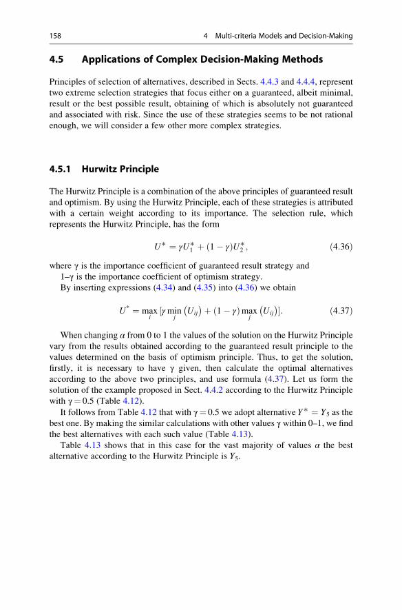
4.5 Applications of Complex Decision-Making Methods
Principles of selection of alternatives, described in Sects. 4.4.3 and 4.4.4, represent
two extreme selection strategies that focus either on a guaranteed, albeit minimal,
result or the best possible result, obtaining of which is absolutely not guaranteed
and associated with risk. Since the use of these strategies seems to be not rational
enough, we will consider a few other more complex strategies.
4.5.1 Hurwitz Principle
The Hurwitz Principle is a combination of the above principles of guaranteed result
and optimism. By using the Hurwitz Principle, each of these strategies is attributed
with a certain weight according to its importance. The selection rule, which
represents the Hurwitz Principle, has the form
U∗ ¼ γU∗1 þ 1� γð ÞU∗
2 ; ð4:36Þwhere γ is the importance coefficient of guaranteed result strategy and
1–γ is the importance coefficient of optimism strategy.
By inserting expressions (4.34) and (4.35) into (4.36) we obtain
U* ¼ maxi
½γminj
Uij
� þ 1� γð Þmaxj
Uij
� �: ð4:37Þ
When changing α from 0 to 1 the values of the solution on the Hurwitz Principle
vary from the results obtained according to the guaranteed result principle to the
values determined on the basis of optimism principle. Thus, to get the solution,
firstly, it is necessary to have γ given, then calculate the optimal alternatives
according to the above two principles, and use formula (4.37). Let us form the
solution of the example proposed in Sect. 4.4.2 according to the Hurwitz Principle
with γ¼ 0.5 (Table 4.12).
It follows from Table 4.12 that with γ¼ 0.5 we adopt alternative Y∗ ¼ Y5 as the
best one. By making the similar calculations with other values γ within 0–1, we findthe best alternatives with each such value (Table 4.13).
Table 4.13 shows that in this case for the vast majority of values α the best
alternative according to the Hurwitz Principle is Y5.
158 4 Multi-criteria Models and Decision-Making
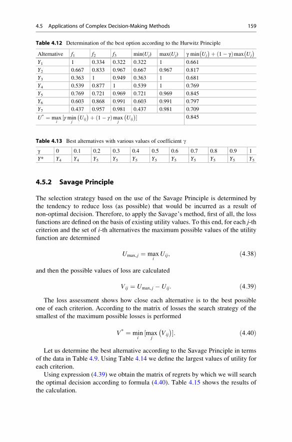
4.5.2 Savage Principle
The selection strategy based on the use of the Savage Principle is determined by
the tendency to reduce loss (as possible) that would be incurred as a result of
non-optimal decision. Therefore, to apply the Savage’s method, first of all, the loss
functions are defined on the basis of existing utility values. To this end, for each j-thcriterion and the set of i-th alternatives the maximum possible values of the utility
function are determined
Umax, j ¼ maxi
Uij; ð4:38Þ
and then the possible values of loss are calculated
Vij ¼ Umax, j � Uij: ð4:39ÞThe loss assessment shows how close each alternative is to the best possible
one of each criterion. According to the matrix of losses the search strategy of the
smallest of the maximum possible losses is performed
V* ¼ mini
½maxj
Vij
� �: ð4:40Þ
Let us determine the best alternative according to the Savage Principle in terms
of the data in Table 4.9. Using Table 4.14 we define the largest values of utility for
each criterion.
Using expression (4.39) we obtain the matrix of regrets by which we will search
the optimal decision according to formula (4.40). Table 4.15 shows the results of
the calculation.
Table 4.12 Determination of the best option according to the Hurwitz Principle
Alternative f1 f2 f3 min(Uj) max(Uj) γ min Uj
� þ 1� γð Þmax Uj
� Y1 1 0.334 0.322 0.322 1 0.661
Y2 0.667 0.833 0.967 0.667 0.967 0.817
Y3 0.363 1 0.949 0.363 1 0.681
Y4 0.539 0.877 1 0.539 1 0.769
Y5 0.769 0.721 0.969 0.721 0.969 0.845
Y6 0.603 0.868 0.991 0.603 0.991 0.797
Y7 0.437 0.957 0.981 0.437 0.981 0.709
U* ¼ maxi
½γminj
Uij
� þ 1� γð Þmaxj
Uij
� � 0.845
Table 4.13 Best alternatives with various values of coefficient g
γ 0 0.1 0.2 0.3 0.4 0.5 0.6 0.7 0.8 0.9 1
Y* Y4 Y4 Y5 Y5 Y5 Y5 Y5 Y5 Y5 Y5 Y5
4.5 Applications of Complex Decision-Making Methods 159
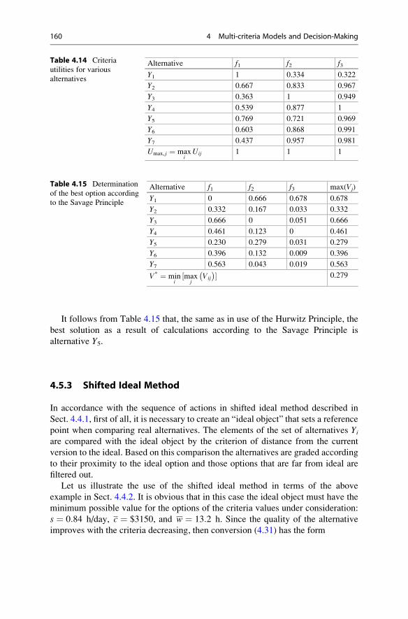
It follows from Table 4.15 that, the same as in use of the Hurwitz Principle, the
best solution as a result of calculations according to the Savage Principle is
alternative Y5.
4.5.3 Shifted Ideal Method
In accordance with the sequence of actions in shifted ideal method described in
Sect. 4.4.1, first of all, it is necessary to create an “ideal object” that sets a reference
point when comparing real alternatives. The elements of the set of alternatives Yiare compared with the ideal object by the criterion of distance from the current
version to the ideal. Based on this comparison the alternatives are graded according
to their proximity to the ideal option and those options that are far from ideal are
filtered out.
Let us illustrate the use of the shifted ideal method in terms of the above
example in Sect. 4.4.2. It is obvious that in this case the ideal object must have the
minimum possible value for the options of the criteria values under consideration:
s ¼ 0:84 h/day, c ¼ $3150, and w ¼ 13:2 h. Since the quality of the alternative
improves with the criteria decreasing, then conversion (4.31) has the form
Table 4.14 Criteria
utilities for various
alternatives
Alternative f1 f2 f3
Y1 1 0.334 0.322
Y2 0.667 0.833 0.967
Y3 0.363 1 0.949
Y4 0.539 0.877 1
Y5 0.769 0.721 0.969
Y6 0.603 0.868 0.991
Y7 0.437 0.957 0.981
Umax, j ¼ maxi
Uij 1 1 1
Table 4.15 Determination
of the best option according
to the Savage Principle
Alternative f1 f2 f3 max(Vj)
Y1 0 0.666 0.678 0.678
Y2 0.332 0.167 0.033 0.332
Y3 0.666 0 0.051 0.666
Y4 0.461 0.123 0 0.461
Y5 0.230 0.279 0.031 0.279
Y6 0.396 0.132 0.009 0.396
Y7 0.563 0.043 0.019 0.563
V* ¼ mini
½maxj
Vij
� � 0.279
160 4 Multi-criteria Models and Decision-Making

aij ¼f ij � f�j� �fþj � f�j� � : ð4:41Þ
Using conversion (4.41) we rate the initial data in Table 4.8 to define the
distances from the ideal object (Table 4.16). For example, for the value of criterion
f 2 ¼ c in option 5 we have
a52 ¼f 52 � f�2� fþ2 � f�2� ¼ 5322� 3150ð Þ
9435� 3150ð Þ ¼ 0:346:
According to Table 4.16, we can calculate the distances of different alternatives
to the ideal object with different metric of criteria space, which is given by
concentration factor p in formula (4.32). If the weights of all the criteria are the
same, then for the i-th alternative formula (4.32) has the form
Lpi ¼ �Xk
j¼1
aijp1=p: ð4:42Þ
For example, for alternative 5 with concentration factor p ¼ 2 we have
L25 ¼�X3j¼1
a25j1=2 ¼ 0:521:
Table 4.17 shows the distances calculated by formula (4.42) for various p values.Obviously, the less the alternative’s distance from the ideal object, the most
preferable it is. Let us grade the preferability of alternatives according to their
proximity to the ideal object for different factors p.For example, for p¼ 1 we have
L15 < L12 < L16 < L14 < L17 < L13 < L11
and accordingly,
Table 4.16 Rated values
of criteria for distance
calculation
Alternative f1 f2 f3
Y1 1 0 1
Y2 0.247 0.498 0.047
Y3 0 1 0.072
Y4 0.182 0.691 0
Y5 0.388 0.346 0.043
Y6 0.194 0.595 0.011
Y7 0.064 0.846 0.025
4.5 Applications of Complex Decision-Making Methods 161

Y5 Y2 Y6 Y4 Y7 Y3 Y1;
where symbolmeans that the value on the left from this symbol is more preferable
than the value on the right.
Analysis of Table 4.17 shows that in this case the sequence is remained even
with all other p. It is, therefore, evident that the smallest deviation from the ideal
object is given by alternative Y5 and it can be accepted as the best. Generally
speaking, such situation occurs not always, i.e. there may be cases when with
various p the grading of alternatives by proximity to the ideal object is different.
In these cases, the graded sequences of alternatives are analysed and the dominated
alternatives are identified, i.e. those that are known not to be the best with all
p values. After excluding such alternatives from consideration a new ideal object
can be formed, and the procedure of grading can be repeated, etc.
In conclusion, we note that for the problem set in Sect. 4.4.2 in most of the
methods of decision-making, alternative Y5 was recognized as the best one, which islikely to be adopted as a solution to this problem.
References
Hugo, M. (2006). Essentials of supply chain management (2nd ed.). Hoboken, NJ: Wiley.
Mauergauz, Y. (1999). Industrial management information systems. Moscow: Filin (in Russian).
Mauergauz, Y. (2012). Objectives and constraints in advanced planning problems with regard to
scale of production output and plan hierarchical level. International Journal of Industrial andSystems Engineering, 12, 369–393.
Minyuk, S. A., Rovba, Y. A., & Kuzmich, K. K. (2002). Mathematical methods and models ineconomy. Minsk: TetraSystems (in Russian).
Missbauer, H. (2002). Lot sizing in workload control systems. Production, Planning & Control,13, 649–664.
Simon, H. A. (1959). Theories of decision-making in economics and behavioural science. TheAmerican Economic Review, 49, 253–283.
Sobol, I. M., & Statnikov, R. B. (1981). Selection of optimal parameters in the problems withmultiple criteria. Moscow: Nauka (in Russian).
T’Kindt, V., & Billaut, J. C. (2005). Multicriteria scheduling. Theory, models and algorithms.Berlin: Springer.
VanWassenhoven, L., & Gelders, L. F. (1980). Solving a bicriterion scheduling problem.
European Journal of Operational Research, 4, 42–48.
Table 4.17 Distances of alternatives to the ideal object with various p values
Alternative
Concentration p
1 2 3 4 5 6 8
Y1 2 1.414 1.259 1.189 1.148 1.122 1.09
Y2 0.792 0.558 0.518 0.506 0.501 0.5 0.499
Y3 1.072 1.002 1 1 1 1 1
Y4 0.873 0.714 0.695 0.692 0.691 0.691 0.691
Y5 0.777 0.521 0.463 0.438 0.424 0.415 0.404
Y6 0.8 0.626 0.601 0.596 0.595 0.595 0.595
Y7 0.935 0.848 0.845 0.845 0.845 0.845 0.845
162 4 Multi-criteria Models and Decision-Making
Data for Planning 5
5.1 Composition of the Data Used for Planning
Planning is the main and most complex business process determining the produc-
tion activities of the enterprise, and therefore its implementation requires the
greatest amount of diverse information. The entire array of necessary information
can be divided into five large groups:
• Archives of design and production documentation
• Archives of orders and contracts
• Reference data
• Databases of transactional information systems
• Databases for decision-making
• Knowledge bases
5.1.1 Archives of Design-Engineering Documentation and Orders
A distinctive feature of the archive information is maintenance of revision history
of the documents in the archive. In other words, every document belonging to the
archive must be presented in all versions of its consistent development. Availability
of archival document in its original form and all its subsequent changes allows
analysing the performance of the enterprise later to improve production and inter-
action with consumers.
The archive of design documentation consists of graphic and text documents,
among which the engineering bills have the primary value for planning. The
structure of engineering bills (Bill of Materials, BOM), as is known, is hierarchical,
where each BOM, on one hand, is included into the supreme bill, and, on the other
hand, includes other bills and individual objects. For the purpose of planning the
BOMs are subject to explosion process, the result of which is to determine the
amount of each design object in the unit of finished production.
# Springer International Publishing Switzerland 2016
Y. Mauergauz, Advanced Planning and Scheduling in Manufacturing and SupplyChains, DOI 10.1007/978-3-319-27523-9_5
163
The archive of production documentation, in contrast to the design archive, is
used almost to the full extent during planning. In planning, the most essential is the
following: content of operations and their sequence, job allocation between the
workshops, norms of material expenditure, equipment and standard time of
operations, personnel requirements and their qualifications, the need for special-
purpose tools, etc.
In the references on planning, the design documentation is usually regarded as a
given set of data, which may even be related to the reference data. In fact,
nowadays, both design and production documentation in a number of industries
are subject to very rapid changes. This is due primarily to market fluctuations and
keen competition, which generates a need for frequent changes in the parameters of
the manufactured products. Furthermore, to meet the market requirements it is
necessary to increase the speed of innovation development, which, of course, leads
to the need for subsequent refinement of products during the manufacturing pro-
cess. As a result, the frequency of changes in production in some cases (especially
in machinery engineering) is increased to an extent that we can talk of a continuous
stream of changes at a certain speed.
Each change in design and production documentation comes into effect in
accordance with the document, which is called a change notice. In different systems
of standardization, this document may have a different form. In view of the special
role of this document in the archive management, we shall consider the work using
the example developed in the Russian system of design documents (Table 5.1). The
change notice can consist of several sheets. This example shows two first sheets of
the notice consisting of seven sheets.
As can be seen from Table 5.1, on the first sheet of the change notice there is the
header of the notice and instructions regarding which products these changes shall
be made and to whom they shall be distributed. If the corrected documents are used
in different items and are used by different subscribers, the instruction on the
applicability and distribution must be recorded for each of the modified documents
separately in the field “Description of change”.
The header indicates the author of the notice, its serial number, reason for
change and its code, release date, and the total number of sheets. If the design
notice entails the need to issue the production notice, both of these notices consti-
tute a single package with a common number. In this case, the design notice has
number 1, and production one—number 2. Attachments to the notice may be new
BOM sheets, drawings, etc.
Table 5.1 presents various cases of changes in engineering bills and drawings.
For example, in bill KK4851.000, a new part “Products manufactured on the
machine KK4851.126 Ring” is entered, “Nut 2M16-6N.21” is replaced by “Nut
AM16-6N.20”, and designation “P73*88*2” is corrected to “P60*5*2”. Upon
replacement or correction, the old records and drawings are recorded in the notice
with strikethrough, as shown in Table 5.1. In the bills the sheets can be cancelled
and new sheets can be introduced; in the parts drawing, dimensions or graphics can
be changed, etc. Serial number of changes in field “Revision” indicates the number
of changes made over the specified line of the bill or part.
164 5 Data for Planning
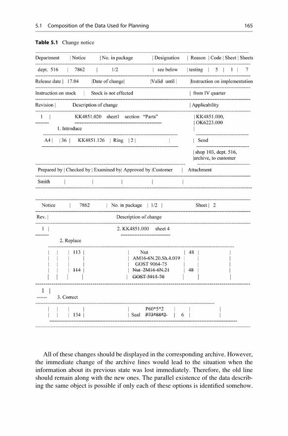
All of these changes should be displayed in the corresponding archive. However,
the immediate change of the archive lines would lead to the situation when the
information about its previous state was lost immediately. Therefore, the old line
should remain along with the new ones. The parallel existence of the data describ-
ing the same object is possible if only each of these options is identified somehow.
Table 5.1 Change notice
5.1 Composition of the Data Used for Planning 165
Usually, every change notice is associated with its own version of the product or
process. This version, as a rule, should include all previous changes that occurred
with this object, i.e. cover the previous change notices. Since the object to be
changed may enter into various kinds of finished product, as shown in Table 5.1,
then even one change can lead to the emergence of new versions of several types of
finished products.
Of course, it does not make sense to keep such a large number of different
versions of the finished product. Therefore, the necessary change notices should be
kept and accounted in explosion, but in this case, it brings the logic question as to
which version should be employed. It is generally believed that only one version is
valid at the current moment and it is called active.
The active version of the finished product material specification and the
corresponding active version of the technological process should be created auto-
matically by the information systems based on primary documentation and the
current notices of change. The latter, however, is not always obvious.
If we look at Table 5.1, we can see that it has two positions determining the
initiation of the notice. The main position is “Instruction on implementation” that
determines the moment of implementation (activation) of the notice. This moment
can be specified by the date, by the number of finished product set, or by such even
not a very specific phrase as “upon wear-out of the mould”. In addition, in Table 5.1
there is position “Instruction on stock”, which may contain information about the
future of previously manufactured objects subject to these changes.
The difficulty of the instruction performance regarding the implementation
and use of the stock greatly complicates the possibility of automatic detection of
activation of a change notice. Therefore, in many cases, if the automatic detection
of the activity of the notice fails, it is necessary to identify information on its
activity manually.
Arrangement of active versions of specifications for products and process is
carried out during preparation for planning of customer order fulfilment according
to the bills of these orders. The order bills are stored in the archives of contracts and
orders and provide data on the amount and time of the shipments of finished
products and other objects to the customers. Each order bill can contain multiple
items (lines) differing in the type of product, date of shipment, special requirements
for products, etc. Preparation of planning should be done if a decision is made on
the performance of a specific position of a specific order. In this case, the specific
active versions of the product and process can be determined based on the
customer’s requirements.
As a result, the so-called Production Process Model (PPM) is created for each
line of the customer order bill. The PPM contains full data on all manufactured
objects, their required quantity, and applied processes. Using the PPM allows
associating each instance of the product with the appropriate version of the design
documentation and thus tracing the influence of this document version on the
quality of the product performance within its lifecycle. The use of production
process model is described in detail below in Chap. 12.
166 5 Data for Planning
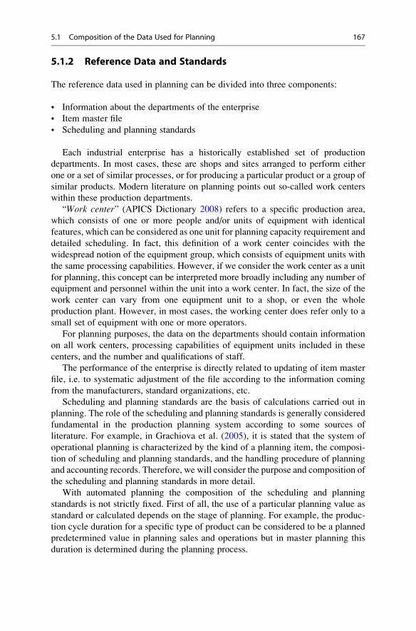
5.1.2 Reference Data and Standards
The reference data used in planning can be divided into three components:
• Information about the departments of the enterprise
• Item master file
• Scheduling and planning standards
Each industrial enterprise has a historically established set of production
departments. In most cases, these are shops and sites arranged to perform either
one or a set of similar processes, or for producing a particular product or a group of
similar products. Modern literature on planning points out so-called work centers
within these production departments.
“Work center” (APICS Dictionary 2008) refers to a specific production area,
which consists of one or more people and/or units of equipment with identical
features, which can be considered as one unit for planning capacity requirement and
detailed scheduling. In fact, this definition of a work center coincides with the
widespread notion of the equipment group, which consists of equipment units with
the same processing capabilities. However, if we consider the work center as a unit
for planning, this concept can be interpreted more broadly including any number of
equipment and personnel within the unit into a work center. In fact, the size of the
work center can vary from one equipment unit to a shop, or even the whole
production plant. However, in most cases, the working center does refer only to a
small set of equipment with one or more operators.
For planning purposes, the data on the departments should contain information
on all work centers, processing capabilities of equipment units included in these
centers, and the number and qualifications of staff.
The performance of the enterprise is directly related to updating of item master
file, i.e. to systematic adjustment of the file according to the information coming
from the manufacturers, standard organizations, etc.
Scheduling and planning standards are the basis of calculations carried out in
planning. The role of the scheduling and planning standards is generally considered
fundamental in the production planning system according to some sources of
literature. For example, in Grachiova et al. (2005), it is stated that the system of
operational planning is characterized by the kind of a planning item, the composi-
tion of scheduling and planning standards, and the handling procedure of planning
and accounting records. Therefore, we will consider the purpose and composition of
the scheduling and planning standards in more detail.
With automated planning the composition of the scheduling and planning
standards is not strictly fixed. First of all, the use of a particular planning value as
standard or calculated depends on the stage of planning. For example, the produc-
tion cycle duration for a specific type of product can be considered to be a planned
predetermined value in planning sales and operations but in master planning this
duration is determined during the planning process.
5.1 Composition of the Data Used for Planning 167
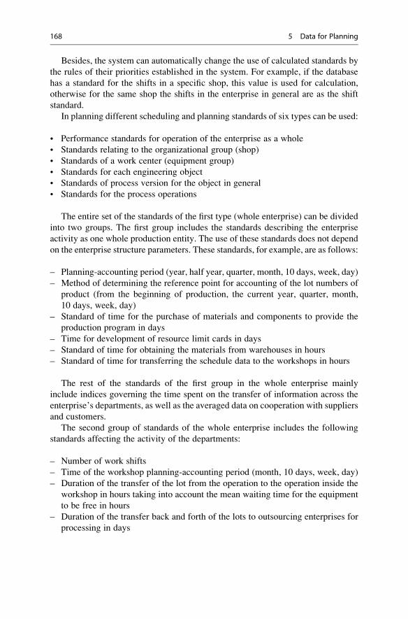
Besides, the system can automatically change the use of calculated standards by
the rules of their priorities established in the system. For example, if the database
has a standard for the shifts in a specific shop, this value is used for calculation,
otherwise for the same shop the shifts in the enterprise in general are as the shift
standard.
In planning different scheduling and planning standards of six types can be used:
• Performance standards for operation of the enterprise as a whole
• Standards relating to the organizational group (shop)
• Standards of a work center (equipment group)
• Standards for each engineering object
• Standards of process version for the object in general
• Standards for the process operations
The entire set of the standards of the first type (whole enterprise) can be divided
into two groups. The first group includes the standards describing the enterprise
activity as one whole production entity. The use of these standards does not depend
on the enterprise structure parameters. These standards, for example, are as follows:
– Planning-accounting period (year, half year, quarter, month, 10 days, week, day)
– Method of determining the reference point for accounting of the lot numbers of
product (from the beginning of production, the current year, quarter, month,
10 days, week, day)
– Standard of time for the purchase of materials and components to provide the
production program in days
– Time for development of resource limit cards in days
– Standard of time for obtaining the materials from warehouses in hours
– Standard of time for transferring the schedule data to the workshops in hours
The rest of the standards of the first group in the whole enterprise mainly
include indices governing the time spent on the transfer of information across the
enterprise’s departments, as well as the averaged data on cooperation with suppliers
and customers.
The second group of standards of the whole enterprise includes the following
standards affecting the activity of the departments:
– Number of work shifts
– Time of the workshop planning-accounting period (month, 10 days, week, day)
– Duration of the transfer of the lot from the operation to the operation inside the
workshop in hours taking into account the mean waiting time for the equipment
to be free in hours
– Duration of the transfer back and forth of the lots to outsourcing enterprises for
processing in days
168 5 Data for Planning
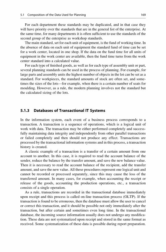
For each department these standards may be duplicated, and in that case they
will have priority over the standards that are in the general list of the enterprise. At
the same time, for many departments it is often sufficient to use the standards of the
second group of the enterprise as workshop standards.
The main standard, set for each unit of equipment, is the fund of working time. In
the absence of data on each unit of equipment the standard fund of time can be set
for a work center, located in one shop. If the data on the fund time for all units of
equipment in the work center are available, then the fund time turns from the work
center standard into a calculated value.
For each type of finished goods, as well as for each type of assembly unit or part,
several planning standards can be used in the process of planning. For example, for
large parts and assembly units the highest number of objects in the lot can be set as a
standard. For workpieces, the standard amounts of stock are often set, and some-
times the sizes of the lots—for example, when there is a certain number of seats for
moulding. However, as a rule, the modern planning involves not the standard but
the calculated sizing of the lots.
5.1.3 Databases of Transactional IT Systems
In the information system, each event of a business process corresponds to a
transaction. A transaction is a sequence of operations, which is a logical unit of
work with data. The transaction may be either performed completely and success-
fully maintaining data integrity and independently from other parallel transactions
or failed completely and then should not produce any effect. Transactions are
processed by the transactional information systems and in this process, a transaction
history is created.
A classic example of a transaction is a transfer of a certain amount from one
account to another. In this case, it is required to read the account balance of the
sender, reduce the balance by the transfer amount, and save the new balance value.
Then it is necessary to read the account balance of the recipient, add the transfer
amount, and save the new value. All these procedures represent one logical unit and
cannot be recorded or processed separately, since this may cause the loss of the
transferred amount. In many cases, for example, when accounting the receipt or
release of the goods, accounting the production operations, etc., a transaction
consists of a single operation.
As a rule, transactions are recorded in the transactional database immediately
upon receipt and this process is called on-line transaction process (OLTP). If the
transaction is found to be erroneous, then the database must allow the user to cancel
or correct this transaction, and it should be possible not only immediately after the
transaction, but after certain and sometimes even long time. In the transactional
database, the incoming source information usually does not undergo any modifica-
tion. These data are not systematized upon receipt and stored in the same format as
received. Some systematization of these data is possible during report preparation.
5.1 Composition of the Data Used for Planning 169
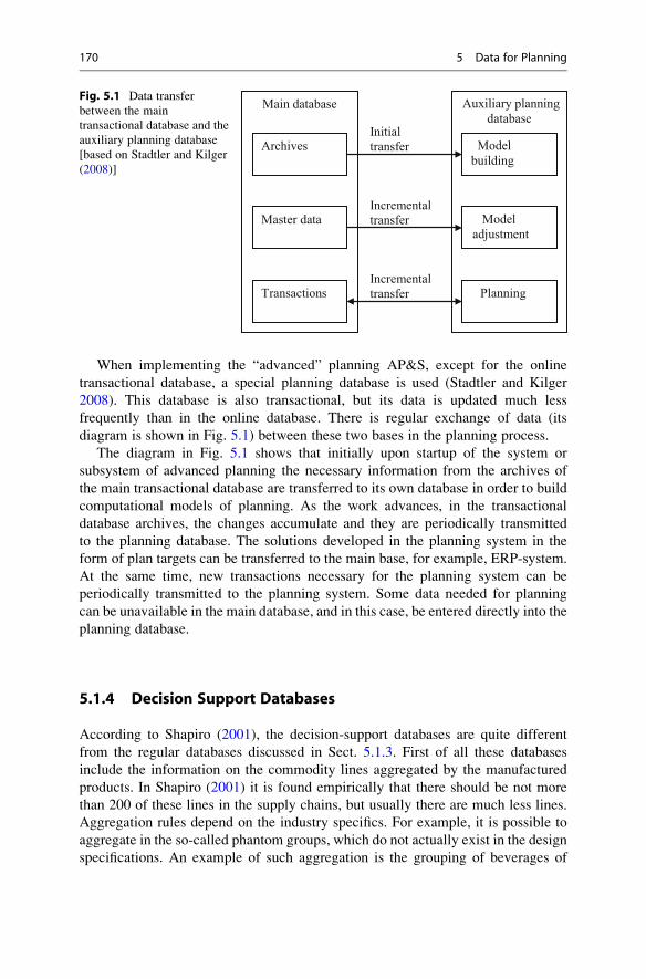
When implementing the “advanced” planning AP&S, except for the online
transactional database, a special planning database is used (Stadtler and Kilger
2008). This database is also transactional, but its data is updated much less
frequently than in the online database. There is regular exchange of data (its
diagram is shown in Fig. 5.1) between these two bases in the planning process.
The diagram in Fig. 5.1 shows that initially upon startup of the system or
subsystem of advanced planning the necessary information from the archives of
the main transactional database are transferred to its own database in order to build
computational models of planning. As the work advances, in the transactional
database archives, the changes accumulate and they are periodically transmitted
to the planning database. The solutions developed in the planning system in the
form of plan targets can be transferred to the main base, for example, ERP-system.
At the same time, new transactions necessary for the planning system can be
periodically transmitted to the planning system. Some data needed for planning
can be unavailable in the main database, and in this case, be entered directly into the
planning database.
5.1.4 Decision Support Databases
According to Shapiro (2001), the decision-support databases are quite different
from the regular databases discussed in Sect. 5.1.3. First of all these databases
include the information on the commodity lines aggregated by the manufactured
products. In Shapiro (2001) it is found empirically that there should be not more
than 200 of these lines in the supply chains, but usually there are much less lines.
Aggregation rules depend on the industry specifics. For example, it is possible to
aggregate in the so-called phantom groups, which do not actually exist in the design
specifications. An example of such aggregation is the grouping of beverages of
Incrementaltransfer
Incrementaltransfer
Initial transfer
Auxiliary planning database
Main database
Archives
Master data
Transactions
Model building
Model adjustment
Planning
Fig. 5.1 Data transfer
between the main
transactional database and the
auxiliary planning database
[based on Stadtler and Kilger
(2008)]
170 5 Data for Planning
various brands by packages of the same standard size. Grouping is also possible
according to customers, suppliers, geographical distribution, etc.
The second direction of organizing data in bases in decision-support databases is
accumulation of information about the location of companies within the supply
chain, about the transport network among these companies, and their available
stocks of aggregated products. The third type of data in these databases includes
information on suppliers of materials, raw materials and components, on the prices
of these goods, and the delivery cost. Finally, the decision-support databases can
record information about the constraints concerning available equipment resources,
finance, personnel, etc.
Decision-support databases are used in analytical information systems. Informa-
tion analysis systems operate using the operational data obtained online from
operational systems that automate the main activities of the company, as well as
other available data sources that may be needed for various decisions. Information
analysis systems are usually an add-on of already functioning data applications at
the enterprise. The systems do not have much influence on their functioning or
require their replacement.
The database, created and used by an analytical information system, in contrast
to conventional transactional databases, is needed not to store the information
about the events but to plan future actions. For this purpose, the information in a
transactional-based is systematized and studied from different perspectives. In
some cases, this information may be insufficient and then additional data may be
entered directly into the decision-support database.
In the paper of Zaratuychenko (1998), the transactional and analytical systems
including their created databases (Table 5.2) were compared. Though this study
was conducted for the banking system, it is fully reflects a similar situation and for
industrial systems.
Analysis of the figures in Table 5.2 indicates that the decision-support database
is a necessary link connecting transactional data with analytical methods of
decision-making. In such a basis the data from different areas of administrative
activity: accounting, planning, operational management, organization of transport
can be collected. The use of the decision-support database for analytical data
processing is discussed below in Sect. 5.2.7. The decision-support database can
serve as a basis for the use of optimization planning models.
5.1.5 Knowledge Bases
Knowledge base is a database of a special kind which is intended to manage
knowledge, i.e. to collect, search, and retrieve the knowledge for use. Knowledge
bases and methods of work with them are studied by the section of Artificial
Intellect (AI) theory, which is called knowledge engineering. The knowledge
base contains various facts and rules of their retrieval from the totality allowing
for logical processing of the information received. For development of knowledge
bases, logic programming languages are mostly used, such as Prolog.
5.1 Composition of the Data Used for Planning 171
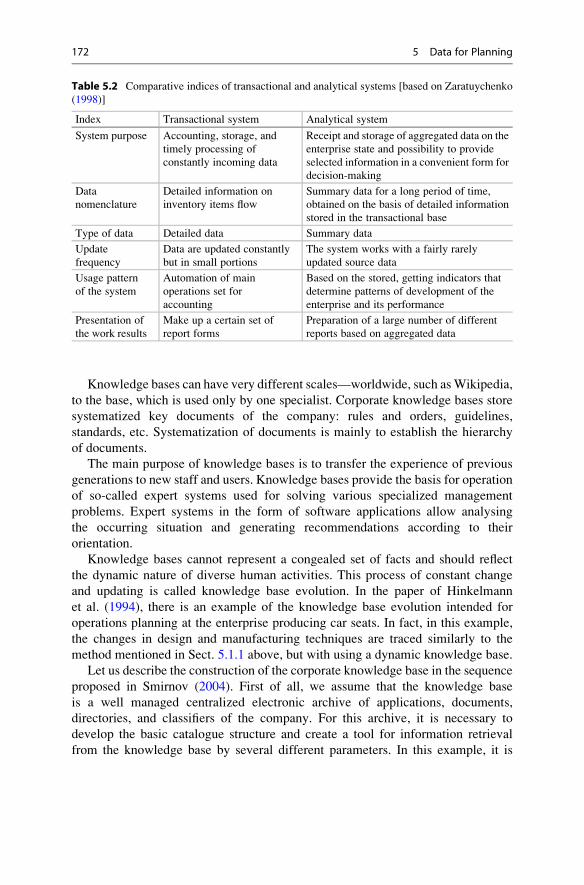
Knowledge bases can have very different scales—worldwide, such asWikipedia,
to the base, which is used only by one specialist. Corporate knowledge bases store
systematized key documents of the company: rules and orders, guidelines,
standards, etc. Systematization of documents is mainly to establish the hierarchy
of documents.
The main purpose of knowledge bases is to transfer the experience of previous
generations to new staff and users. Knowledge bases provide the basis for operation
of so-called expert systems used for solving various specialized management
problems. Expert systems in the form of software applications allow analysing
the occurring situation and generating recommendations according to their
orientation.
Knowledge bases cannot represent a congealed set of facts and should reflect
the dynamic nature of diverse human activities. This process of constant change
and updating is called knowledge base evolution. In the paper of Hinkelmann
et al. (1994), there is an example of the knowledge base evolution intended for
operations planning at the enterprise producing car seats. In fact, in this example,
the changes in design and manufacturing techniques are traced similarly to the
method mentioned in Sect. 5.1.1 above, but with using a dynamic knowledge base.
Let us describe the construction of the corporate knowledge base in the sequence
proposed in Smirnov (2004). First of all, we assume that the knowledge base
is a well managed centralized electronic archive of applications, documents,
directories, and classifiers of the company. For this archive, it is necessary to
develop the basic catalogue structure and create a tool for information retrieval
from the knowledge base by several different parameters. In this example, it is
Table 5.2 Comparative indices of transactional and analytical systems [based on Zaratuychenko
(1998)]
Index Transactional system Analytical system
System purpose Accounting, storage, and
timely processing of
constantly incoming data
Receipt and storage of aggregated data on the
enterprise state and possibility to provide
selected information in a convenient form for
decision-making
Data
nomenclature
Detailed information on
inventory items flow
Summary data for a long period of time,
obtained on the basis of detailed information
stored in the transactional base
Type of data Detailed data Summary data
Update
frequency
Data are updated constantly
but in small portions
The system works with a fairly rarely
updated source data
Usage pattern
of the system
Automation of main
operations set for
accounting
Based on the stored, getting indicators that
determine patterns of development of the
enterprise and its performance
Presentation of
the work results
Make up a certain set of
report forms
Preparation of a large number of different
reports based on aggregated data
172 5 Data for Planning
demonstrated how the entire knowledge base can be developed using only MS
Excel.
In the directory structure, not more than three hierarchical levels should be used,
although it is usually advisable to confine to two levels. For each independent
project of the company, it is recommended to create a separate directory, in which
technical and organizational documents should be separated by subdirectories.
Separate directories are made for regulatory documents, for partners, catalogues
of products, etc. The directories are coded with reference numbers.
Into the reference directories, it is advisable to place such reference files as the
organizational structure of the company, main provisions and regulations, staff
catalogue with phone numbers, customer and partner catalogues, etc. The main
directories of the knowledge base should be filled gradually by sending documents
within the company through the knowledge base. With the course of time, the
knowledge base will be sufficiently complete, and most of the current activity of the
company can be done by referring to the knowledge base and retrieving information
from this database.
As an example of the use of the knowledge base the intelligent system (Kargin
and Mironenko 2008) can be used to automate accounting and planning of produc-
tion (metal cutting) for blank production shops of Mariupol Heavy Machinery Plant
(Ukraine), shown by diagram in Fig. 5.2.
As can be seen from Fig. 5.2, the data from different user groups (supervisors,
engineers, technical departments, site foreman, planners, etc.) get into the
accounting and planning system. These data are then stored in the transactional
database of the system and also get into the intelligent planning system. In block of
problematic situation analysis, the most appropriate (similar) use case (or use
cases) for the current situation is searched and derived from the knowledge base.
For this purpose, the algorithm of the current situation identification is used on the
basis of the algorithm for determining the similarity level between the current
situation and that of the knowledge base. The planner uses the received data for
scheduling.
Another example of the knowledge can be the so-called bank of analytical
models proposed in Novitsky (2010). This article deals with the planning of work
processes with grain when it is stored in elevators and used by flour and feed mills.
The bank of models is a set of mathematical models (usually in the form of
formulas) in the process of selection and allocation of resources in raw materials
procurement, production, sales, and shipment.
For example, such models are the calculated relationships for the cost of
raw materials, sales, profit margins, etc. These calculated values can serve as the
optimization criteria (objective functions) of grain treatment processes. Other
models, such as evaluating the quality of the grain, can be used as constraints in
the calculations. The relevant set of functions from the bank of models allows
performing various business processes: planning grain trade, definition of grinding
mixtures recipes, calculation of feed recipes, etc.
5.1 Composition of the Data Used for Planning 173
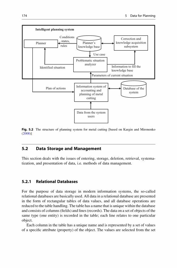
5.2 Data Storage and Management
This section deals with the issues of entering, storage, deletion, retrieval, systema-
tization, and presentation of data, i.e. methods of data management.
5.2.1 Relational Databases
For the purpose of data storage in modern information systems, the so-called
relational databases are basically used. All data in a relational database are presented
in the form of rectangular tables of data values, and all database operations are
reduced to the table handling. The table has a name that is unique within the database
and consists of columns (fields) and lines (records). The data on a set of objects of the
same type (one entity) is recorded in the table; each line relates to one particular
object.
Each column in the table has a unique name and is represented by a set of values
of a specific attribute (property) of the object. The values are selected from the set
Information to fill the knowledge base
rules
Conditions
, states,Planner’s
knowledge base
Correction andknowledge acquisition
subsystem
Problematic situation analyzer
Planner
Identified situation
Information system of accounting and
planning of metal
cutting
Use case
Database of the system
Data from the system users
Parameters of current situation
Plan of actions
Intelligent planning system
Fig. 5.2 The structure of planning system for metal cutting [based on Kargin and Mironenko
(2008)]
174 5 Data for Planning
of all possible values of the object’s attribute, which is called domain. In the
simplest case, a domain is defined as the admissible potential set of values of the
same type. For example, a set of dates of birth of all employees contains “domain of
dates of birth” and the names of all employees are “domain names of employees”.
Domain of dates of birth has the data type that allows you to store information about
moments of time, and the domain of employee names must have the character
data type.
Each table should have a primary key—a field or set of fields, content of which
unambiguously defines the record in the table and sets it apart from others.
Communication (foreign key) between two tables is usually formed when added
to the first table field containing the primary key value of the second table.
Tables should be organized in such a way to eliminate duplication of data in the
tables and ensure their consistency. The process of this organization is called
relation normalization between tables.
Let us consider the process of normalization in the example with suppliers and
supply of goods. Suppose that we need to store information about the names of the
suppliers, the names and quantity of the goods supplied, at that each supplier can
supply several products of various kinds, and each item of one type can be supplied
by several suppliers. Obviously, there is a relation between suppliers and goods that
determines what goods can be delivered by each supplier. This relationship is rather
complicated, because it is a connection between the two sets. This type of connec-
tion is called a “many-to-many” and cannot be properly reflected in the relational
database directly.
In the relational databases, “one-to-many” interrelations are basic and “many-to-
many” interrelations implemented by using several “one-to-many” interrelations.
In this case, for example, there is “one-to-many” interrelation between the supplier
and the supplier’s deliveries since one supplier can make several deliveries, in each
of which the products of any possible type can be supplied. Similarly, the same
relation also occurs between the product of one type and deliveries, since one
product can be supplied many times and by different suppliers.
The table being part of the relationship from side “one” (e.g. “Suppliers”) is
called a parent. The table being part of the relationship from side “many”
(e.g. “Shipments”) is called a child. Mechanism for implementing relationship
“one-to-many” is that the child table is added with attributes, which are references
to the key attributes of the parent table. Thus, in the above example there should be
two parent tables (Tables 5.3 and 5.4) and one child table (Table 5.5).
In Table 5.5, attributes “Supplier code” and “Goods Code” are references to the
primary key attributes in Tables 5.3 and 5.4 and therefore, are foreign keys. Using
foreign keys, you can connect Tables 5.3 and 5.4 when retrieving information from
Table 5.5. Real relational tables that describe the mechanism of shipments account-
ing, of course, include significantly more information than given in Table 5.5. The
management of these tables will be discussed below in Sect. 5.2.3.
5.2 Data Storage and Management 175
5.2.2 Concept of Object-Oriented Databases
In addition to relational databases, in recent years, the use of so-called object-
oriented databases based on the object concept of information management has
begun. Object-oriented approach is based on the following concepts:
• Objects and object identifiers
• Attributes and methods
• Classes
• Hierarchy and inheritance of classes
Term “object” means the combination of “data” and “program”, representing a
certain real-world essence. The data consist of the components of arbitrary type
called “attributes”. Each program in the software is called “method”. In the object
concept, it is considered that the object “encapsulates” the data and program. In
other words, users cannot see the inside of the object, but they may use it by
referring to the part of its software.
All objects that have the same attributes (properties), and the same methods are
collectively known as a class and same object should correspond to only one class.
As an example of a class, we can name a set of mobile telephones. In this case, the
object is any unidentified element of this set with all the characteristic properties
Table 5.3 Suppliers Supplier code Supplier name
1 Base “Building”
2 Construction materials store
3 Construction market
4 Plant of lighting engineering
Table 5.4 Goods Goods code Goods name
1 Paint
2 Cement
3 Linoleum
4 Lighting fixture
Table 5.5 Shipments
Supplier code Goods code Quantity Measurement unit
1 1 100 kg
1 2 2 ton
1 3 12 roll
2 1 150 kg
2 2 1.5 ton
3 3 10 roll
4 4 15 pcs.
176 5 Data for Planning
(size, colour, functions, etc.). The description of the object (encapsulation) may
include the program of some actions with the object (on, off, set of messages, etc.).
Each physical element (object) of this set is called an instance. Figure 5.3 shows the
relationship of the class, corresponding object and instance.
Some classes may inherit attributes and methods from other classes. In general,
the class can inherit properties from one or more existing classes and thereby
forming structure of inheritance is called “hierarchy of classes”.
Since the inheritance makes it possible to share the various classes of one set of
attributes and methods, the same program can work with the objects belonging to all
these classes. For example, the object-oriented user interface of software is based
on this. The same set of programs (open, close, new, delete, move, etc.) can be used
to manage different types of data (image, text, graphics, directory, etc.).
In general, the use of object-oriented databases can lead to significant improve-
ment of operational properties of databases with large amounts of information:
increased search speed, possibility of using not only two-dimensional but multidi-
mensional tables, etc. However, nowadays the use of these databases is limited.
5.2.3 Database Management Systems
The software designed to work with databases is Database Management System
(DBMS). DBMS is a shell, which is used to generate a certain database in process of
table structure organization and filling the tables with data. DBMS is used for the
well-ordered storage and processing large amounts of data so that it is convenient to
view, fill, modify and look for the necessary information, draw any samples and sort
in any order.
Relational database management system is based on the relational data model. In
a relational data model, as mentioned above in Sect. 5.2.1, any representation of the
data is reduced to a set of relational tables.
DBMS must meet the requirements such as high performance, easiness
of updating, ability to multi-user use, security, and others. The ability to meet
Set ofA set of items of the sameuse with similar functions(methods)
Class
Typical abstract element of aset, reflecting the properties of a class
Object
Specific instance of the class with own
characteristics
Item
ModelComposition
properties
Fig. 5.3 Relationship of classes, objects, and instances
5.2 Data Storage and Management 177
these requirements is largely provided by the basic database language, which is
Structured Query Language (SQL).
SQL statements look like normal English sentences, which facilitates their
learning and understanding. SQL is the language of interactive queries to a rela-
tional database, which provides users with immediate access to data. With SQL, the
user can interactively get answers to the most complex queries in a split second.
Despite the fact that there is a wide variety of databases, in practice only a few
well-known databases (Oracle, Microsoft SQL, Informix, Interbase, Sybase and
others) are used in manufacturing information systems. Above all, this situation is
due to the huge cost of development of high-quality DBMS, as well as difficulties in
its implementation, support, etc.
Database management system MS Access takes a special place among all
DBMS. Generally speaking, this DBMS cannot be used to construct a complete
information system because it does not provide a reliable multi-user usage of data.
On the other hand, the wide availability of the DBMS allows ordinary users to build
their databases for personal use. Therefore, a number of information systems enable
users to upload data from a powerful network DBMS into MS Access and then work
with the obtained data on a local computer.
5.2.4 Tiered Data Storage
In most such cases, the arrival rate of transactions is such that we can speak of a
certain intensity of the transactions flow. If the intensity is high, then over time
the amount of data in the transactional base can become very large. In this case, a
logic question arises as to the retention period of the data on transactions. It is
usually assumed that since it is usually not possible to determine the necessary
retention period then it is necessary to arrange storage of information in several tiers
(Fig. 5.4).
Figure 5.4 shows that manufacturing data flow enters the pre-set database. These
data are analysed and presented in the form of reports and sent to the short-term
storage archive. This archive data are sorted to the data to be sent to the long-term
storage and the data of no value to store. The first group of data is transferred to
the long-term storage archive, and the data of the second group are deleted. In the
archives of long-term storage, the data are compressed into special CSV-files to
reduce the amount of required memory. The files are text files in which the data are
separated by commas (Comma Separated Values, CSV).
Feasibility of replacement of a relational database by a plurality of CSV files is
due to the fact that each database field is assigned to a certain number of characters,
although the actual data always occupy only part of the space allocated to them. In
the CSV-file, each data value occupies the memory volume exactly corresponding
to the value, which significantly reduces the need for total memory.
178 5 Data for Planning
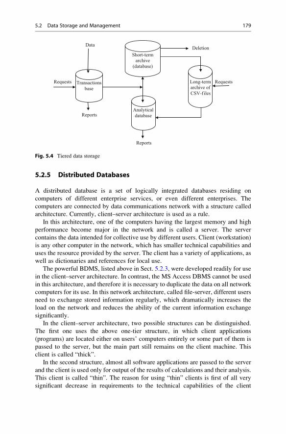
5.2.5 Distributed Databases
A distributed database is a set of logically integrated databases residing on
computers of different enterprise services, or even different enterprises. The
computers are connected by data communications network with a structure called
architecture. Currently, client–server architecture is used as a rule.
In this architecture, one of the computers having the largest memory and high
performance become major in the network and is called a server. The server
contains the data intended for collective use by different users. Client (workstation)
is any other computer in the network, which has smaller technical capabilities and
uses the resource provided by the server. The client has a variety of applications, as
well as dictionaries and references for local use.
The powerful BDMS, listed above in Sect. 5.2.3, were developed readily for use
in the client–server architecture. In contrast, the MS Access DBMS cannot be used
in this architecture, and therefore it is necessary to duplicate the data on all network
computers for its use. In this network architecture, called file-server, different users
need to exchange stored information regularly, which dramatically increases the
load on the network and reduces the ability of the current information exchange
significantly.
In the client–server architecture, two possible structures can be distinguished.
The first one uses the above one-tier structure, in which client applications
(programs) are located either on users’ computers entirely or some part of them is
passed to the server, but the main part still remains on the client machine. This
client is called “thick”.
In the second structure, almost all software applications are passed to the server
and the client is used only for output of the results of calculations and their analysis.
This client is called “thin”. The reason for using “thin” clients is first of all very
significant decrease in requirements to the technical capabilities of the client
RequestsRequests Transactions
base
Short-term archive
(database)
Analytical
database
Data
Reports
Deletion
Long-term archive of
CSV-files
Reports
Fig. 5.4 Tiered data storage
5.2 Data Storage and Management 179
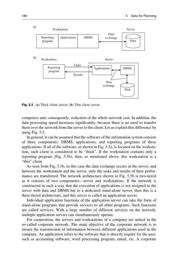
computers and, consequently, reduction of the whole network cost. In addition, the
data processing speed increases significantly, because there is no need to transfer
them over the network from the server to the client. Let us explain this difference by
using Fig. 5.5.
In general, it can be assumed that the software of the information system consists
of three components: DBMS, applications, and reporting programs of these
applications. If all of the software, as shown in Fig. 5.5a, is focused on the worksta-
tion, such client is considered to be “thick”. If the workstation contains only a
reporting program (Fig. 5.5b), then, as mentioned above, this workstation is a
“thin” client.
As seen from Fig. 5.5b, in this case the data exchange occurs in the server, and
between the workstation and the server, only the tasks and results of their perfor-
mance are transferred. The network architecture shown in Fig. 5.5b is two-tiered
as it consists of two components—server and workstations. If the network is
constructed in such a way that the execution of applications is not assigned to the
server with data and DBMS but to a dedicated stand-alone server, then this is a
three-tiered architecture, and this server is called an application server.
Individual application functions of the application server can take the form of
stand-alone programs that provide services to all other programs. Such functions
are called services. With a large number of different services on the network,
multiple application servers can simultaneously operate.
For cooperation, the servers and workstations of a company are united in the
so-called corporate network. The main objective of the corporate network is to
ensure the transmission of information between different applications used in the
company. An application refers to the software that is directly require for the user,
such as accounting software, word processing program, email, etc. A corporate
Reporting program
Applications DBMS
Workstation
Data
Server
Data
exchange
a)
Reporting program
Data
DBMSApplicationsTasks
Data exchange
b)Workstation Server
Results
Fig. 5.5 (a) Thick client–server; (b) Thin client–server
180 5 Data for Planning

network provides for interaction of the applications, located in different geographi-
cal areas, and access for remote users. The compulsory component of the corporate
network is local networks connected to each other.
To maintain the corporate network the regular network administration is
required. The network administration should provide variety of functions. The
objectives are implementation of various changes in the structure of the network,
such as connection of new workstations, configuration of network communication
protocols, setup of network access services, troubleshooting, etc. An important
function of administration is to ensure data security and protection against unau-
thorized access. Data protection includes a number of different tasks: backup and
data recovery, development and change of passwords, wireless security, etc.
5.2.6 Service Oriented Architecture of IT Systems
Since modern software applications can rarely operate in isolation, the application
usually cannot do anything significant without interaction with other applications.
Currently, the construction of enterprise information systems increasingly involves
the so-called service-oriented architecture (SOA). Service-oriented architecture
integrates applications for collaboration and accelerates their operation by breaking
an application into parts that can be combined with each other.
Term SOA refers to the modular approach to software development using
services (utilities) with standardized interfaces. A service refers to an independent
software component that performs a specific task, such as “check credit card”, which
does not require some mandatory software technology to be used by customers.
SOA is characterized by three important properties
• Each service implements a single business-function that is logically distinct,
repetitive task being an integral part of an enterprise business process.
• Services are components of the information system that interact with other
components only through their interfaces due to the use of open, widely used
standards. Service interfaces are independent of platforms, programming
language, operating system, and other technical features of implementation;
services interact with each other and support other services.
• Services in the systems based on SOA can be performed irrespective of other
system services, it is only necessary to know the interface of the used services.
The setup of a set of services for business processes is called “orchestration”.
The SOA usage requires a special technology for integration of services, which, in
contrast to software, is called middleware.
This technology is the basis for the environment of distributed information
processing. Middleware is a class of programs located between the application
layer and system network layer and managing the interaction of applications on
different computing platforms. Most packages of the middleware support high-
level programming interface and a set of services types (such as authentication,
5.2 Data Storage and Management 181
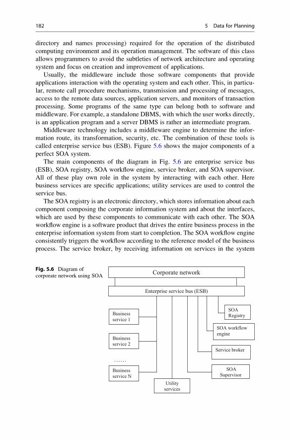
directory and names processing) required for the operation of the distributed
computing environment and its operation management. The software of this class
allows programmers to avoid the subtleties of network architecture and operating
system and focus on creation and improvement of applications.
Usually, the middleware include those software components that provide
applications interaction with the operating system and each other. This, in particu-
lar, remote call procedure mechanisms, transmission and processing of messages,
access to the remote data sources, application servers, and monitors of transaction
processing. Some programs of the same type can belong both to software and
middleware. For example, a standalone DBMS, with which the user works directly,
is an application program and a server DBMS is rather an intermediate program.
Middleware technology includes a middleware engine to determine the infor-
mation route, its transformation, security, etc. The combination of these tools is
called enterprise service bus (ESB). Figure 5.6 shows the major components of a
perfect SOA system.
The main components of the diagram in Fig. 5.6 are enterprise service bus
(ESB), SOA registry, SOA workflow engine, service broker, and SOA supervisor.
All of these play own role in the system by interacting with each other. Here
business services are specific applications; utility services are used to control the
service bus.
The SOA registry is an electronic directory, which stores information about each
component composing the corporate information system and about the interfaces,
which are used by these components to communicate with each other. The SOA
workflow engine is a software product that drives the entire business process in the
enterprise information system from start to completion. The SOA workflow engine
consistently triggers the workflow according to the reference model of the business
process. The service broker, by receiving information on services in the system
Corporate network
Enterprise service bus (ESB)
SOARegistry
SOA workflow
engine
Service broker
SOASupervisor
Utility services
Business
service 1
Business service 2
Business service N
……
Fig. 5.6 Diagram of
corporate network using SOA
182 5 Data for Planning
from the SOA registry, coordinates their work with the SOA workflow engine. The
SOA supervisor monitors the operation of various components within the system,
evaluates the correctness of their functioning, and tracks the requests sent to
external systems.
As can be seen from Fig. 5.6, all software of SOA is connected to the service
bus. Interaction of services via the bus is only possible if certain service level
agreements (SLA) are performed. The quality of services communication can be
evaluated by a set of key performance indicators (KPI) similar to indicators used in
business.
The diagram of group services in Fig. 5.6, presented a chain, can be extended to
the concept of “manufacturing chain” that provided transmission of information
between related production facilities. For example, in the article of Biennier
et al. (2007) ESB, which takes into account a number of production constraints,
is manufacturing service bus (MSB). In the latter, the manufacturing services are
combined with dynamic monitoring system and transfer information between
manufacturing control elements.
5.2.7 On-Line Analytical Processing
Section 5.2.3 described the queries to the relational database, which is the basic
method of information retrieval from the database. If the query is quite simple,
it is performed within seconds. However, in case of complex queries with many
conditions the performance time increases dramatically. Moreover, in analysis of
data, it becomes necessary to perform several (sometimes many), different complex
queries that also require considerable time.
To speed up the analysis of large databases it is possible to prepare the existing
database that allows you to pre-aggregate data in different directions (dimensions).
In fact, in process of this preparation the relational database is transformed into a
sort of database for decision-making described above in Sect. 5.1.4. For analytical
work with such database the special technology was developed. It is called on-line
analytical processing (OLAP), in which the base itself is called “data warehouse”.
While the conventional databases are subject to constant changes in process of
users’ work, the data warehouse is relatively stable: its data are usually updated
according to the schedule (e.g. weekly, daily, or hourly—as needed). Ideally, the
process of filling is simply the addition of new data of a certain period without
changing the previous information already stored in the data warehouse.
Unlike the relational database consisting of flat tables, the OLAP data warehouse
is a data model organized in the form of multidimensional cubes. The axes of the
multidimensional coordinate system are the main attributes of the business process
under consideration. For example, for sales it may be goods, area, types of cus-
tomer. Time can be used as one of measurements. At the intersections of the axes
(dimensions) there are the data (measures) characterizing the process quantita-
tively. These data may be represented by sales volume in pieces or in monetary
terms, stock balance, costs, etc. During the analysis the user can receive
5.2 Data Storage and Management 183
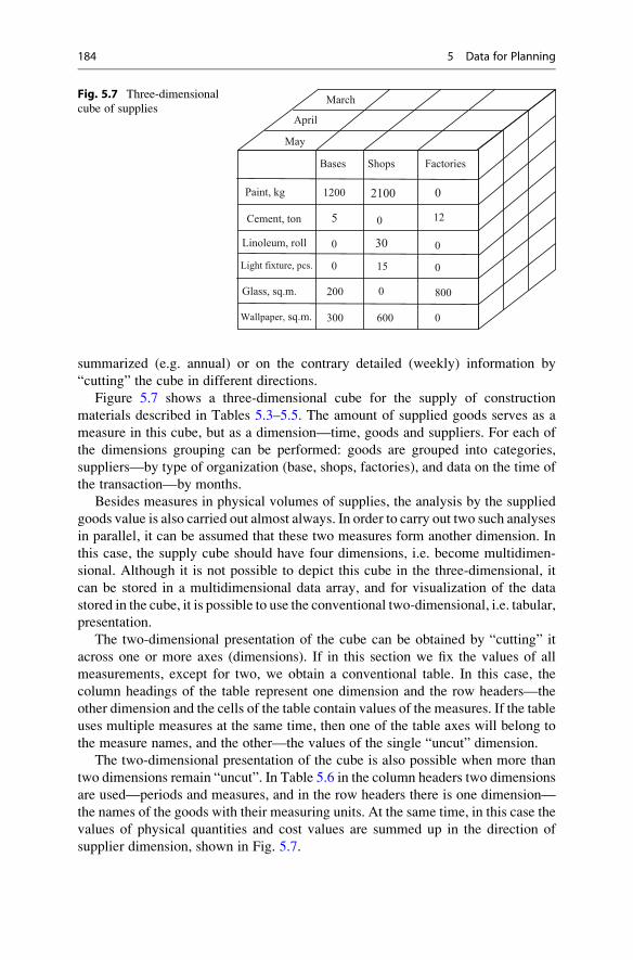
summarized (e.g. annual) or on the contrary detailed (weekly) information by
“cutting” the cube in different directions.
Figure 5.7 shows a three-dimensional cube for the supply of construction
materials described in Tables 5.3–5.5. The amount of supplied goods serves as a
measure in this cube, but as a dimension—time, goods and suppliers. For each of
the dimensions grouping can be performed: goods are grouped into categories,
suppliers—by type of organization (base, shops, factories), and data on the time of
the transaction—by months.
Besides measures in physical volumes of supplies, the analysis by the supplied
goods value is also carried out almost always. In order to carry out two such analyses
in parallel, it can be assumed that these two measures form another dimension. In
this case, the supply cube should have four dimensions, i.e. become multidimen-
sional. Although it is not possible to depict this cube in the three-dimensional, it
can be stored in a multidimensional data array, and for visualization of the data
stored in the cube, it is possible to use the conventional two-dimensional, i.e. tabular,
presentation.
The two-dimensional presentation of the cube can be obtained by “cutting” it
across one or more axes (dimensions). If in this section we fix the values of all
measurements, except for two, we obtain a conventional table. In this case, the
column headings of the table represent one dimension and the row headers—the
other dimension and the cells of the table contain values of the measures. If the table
uses multiple measures at the same time, then one of the table axes will belong to
the measure names, and the other—the values of the single “uncut” dimension.
The two-dimensional presentation of the cube is also possible when more than
two dimensions remain “uncut”. In Table 5.6 in the column headers two dimensions
are used—periods and measures, and in the row headers there is one dimension—
the names of the goods with their measuring units. At the same time, in this case the
values of physical quantities and cost values are summed up in the direction of
supplier dimension, shown in Fig. 5.7.
April
March
May
Paint, kg
Cement, ton
Linoleum, roll
Light fixture, pcs.
Glass, sq.m.
Wallpaper, sq.m.
Bases Shops Factories
1200 2100 0
5 120
30 00
00 15
200 0 800
600 0300
Fig. 5.7 Three-dimensional
cube of supplies
184 5 Data for Planning

Values plotted along the dimensions are known as marks. For example, period
marks may be words “March”, “April”, “May”. Marks are used for “cutting” the
cube and for the restriction (filtering) of the selected data as well if for analysis
instead of all values their subset is used, for example, 3 months of several tens. The
marks values are displayed in the two-dimensional presentation of the cube as row
and column headers. The marks may join into hierarchies, consisting of one or
several levels. For example, the marks of dimension “Shops” naturally join into the
hierarchy with levels:
Worldwide
Country
Area
City
Shop
The data can be aggregated by each of the levels.
Multidimensionality in OLAP application can be divided into three levels
(Alperovich 2001).
• Multidimensional data presentation is means for the end user. It provides
multidimensional visualization and manipulation of data. At that the multidi-
mensional presentation layer is abstracted from the physical structure of data and
accepts data as multidimensional.
• Multidimensional processing is means (language) for multidimensional queries
formulation. Since this language is different from relational language SQL, you
need a processor which can process and perform a multidimensional query.
• Multidimensional storage is means of physical organization of data to ensure the
effective performance of multidimensional queries.
All OLAP tools, for example Pivot Table Service from Microsoft provide
first two levels of the multidimensional presentations. The third level although
being widely spread is optional as the data for the multidimensional presentation
can be retrieved from regular relational data structures as well. Multidimensional
storage allows treating the data as a multidimensional array, and due to this the
equally quick calculations of summarized indices and various multidimensional
conversions of any dimension are provided. However, for the purpose of the
Table 5.6 Example of two-dimension table presenting three dimensions
Goods
March April May
Quantity Cost Quantity Cost Quantity Cost
Paint, kg 500 6000 1100 13,800 3300 34,000
Cement, ton 10 12,000 8 98,000 17 163,000
Linoleum, roll 0 0 20 1580 30 2300
Light fixture, pcs. 0 0 0 0 15 1900
5.2 Data Storage and Management 185

multidimensional storage there should be special multidimensional databases,
which dramatically increase the required volume for storage and the system cost.
5.3 Information Exchange
Currently, the efficient manufacturing activity of an enterprise is possible only if
there is close and most important quick cooperation with other companies, which
create the so-called enterprise network together. As companies has been able
to involve resources and manufacturing capabilities of practically any enterprise
around the world for their own business, the enterprise network can be created for
short-term cooperation as well and have a variable composition.
The enterprise network includes three different flows—material, financial, and
informational and the latter always accompanies the rest. Therefore, it is clear that
for effective collaboration in the network the enterprises must have a set of methods
and related tools providing complete exchange of necessary information.
5.3.1 Internal Data Communication
The issues of data exchange between the information systems available at the
enterprise have been covered quite in details above in Chap. 1. In particular,
Table 1.8 showed five information exchange levels and for the top three layers
the corresponding standards have been described in Sect. 1.5. Here we will discuss
the most common current standard of information processing for level 1, i.e. for the
transmission level of raw information received from various sensors on the equip-
ment to the supervisory system SCADA.
OPC (OLE for Process Control) is the industrial standard developed by a
consortium of world-famous producers of hardware and software with the partici-
pation of Microsoft. This standard describes the communication interface between
the process control devices. The main purpose of the standard was to provide
developers of the dispatch systems some independence from a particular type of
controller. Acronym OLE (Object linking and embedding) is used to denote data
transfer technology in the systems developed by Microsoft, for example, to transfer
data from MS Word to MS Excel and back.
As this name OPC implies, this technology is a way of distributing OLE
technology to processing of the information used for industrial process control.
Development of OPC standard is carried out by OPC Foundation. The OPC
standard clearly delineates responsibilities among hardware manufacturers and
developers of data transfer drivers and this allows you to collect data from various
sources and send them to any client application regardless of the type of equipment
used. As a result, modification of the equipment or production of new items on this
equipment does not require changing the raw information processing programs. In
addition, there is a wide choice of equipment suppliers, as well as possibility to
integrate this equipment in the enterprise information system.
186 5 Data for Planning
The OPC standard includes a number of so-called OPC specifications, the most
common of which are Data Access specifications providing access to data online.
These specifications are used to obtain the following types of data:
• Data from online sensors (temperature, pressure, etc.)
• Control actions (open, close, start, stop, etc.);
• Information about the current status of equipment and executive programs
The OPC technology always involves two computer programs: OPC server and
OPC client. The first provides its functionality through user interfaces and the
second requests and receives the information. The OPC server may be provided
for a controller, I/O card, field bus adapter, conversion program, random number
generator, i.e. any device, transmitting or receiving data. The OPC client is usually
included in the scope of software packages SCADA.
There are three main ways for the OPC client to obtain data from the OPC server:
synchronous reading, asynchronous reading, and subscription. When reading
synchronously the client sends a request to the server with a list of the
manufacturing process parameters required at the moment and waits for the server
to execute it. During asynchronous reading, the client sends a request to the server
and continues to work. When the server fulfils the request, the client receives a
notification. In the case of a subscription, the client sends the server a list of
manufacturing process parameters in interest, and the server then sends the infor-
mation of the changed variables from this list to the client regularly.
5.3.2 Data Transfer Between Enterprises
Information exchange in a production network is defined by two factors—the extent
of information transfer and its intensity. Information extent is determined by the
number of stages of information transfer from the place of its origin to the last in the
enterprise information chain in the production network. Let us consider once more
the commonly used example of the diaper supply chain by Proctor&Gamble for
large retail network Metro, which has been shown above in Fig. 1.2.
As in the case in Fig. 1.2, the production has three stages of supplies and the sales
have two stages, the extent of information transfer from the sales towards the
production—up the supply chain—is three and the extent from the production
towards the sales—down the chain—is two. It should be noted that in reality any
enterprise participates in a number of supply chains, in which the extent of
information transfer can be quite different.
The information intensity describes the amount of information per time unit
transferred via the network. For the supply chain, the entire amount of information
can be classified into six categories (Huang et al. 2003): products, processes,
resources, stocks, orders, and plans (Table 5.7).
The amount of transmitted data, its content, and even the structure of the
production network may change over time. The life cycle of the network can be
5.3 Information Exchange 187
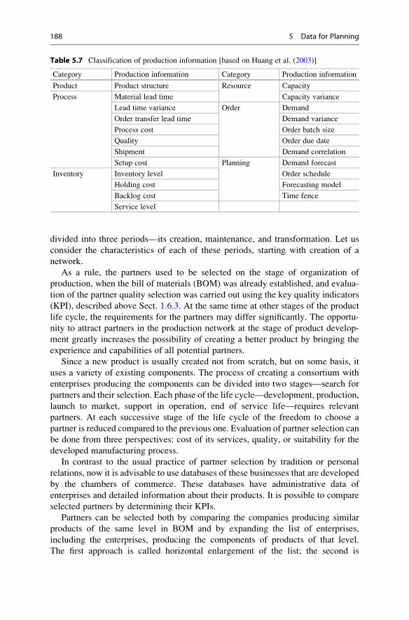
divided into three periods—its creation, maintenance, and transformation. Let us
consider the characteristics of each of these periods, starting with creation of a
network.
As a rule, the partners used to be selected on the stage of organization of
production, when the bill of materials (BOM) was already established, and evalua-
tion of the partner quality selection was carried out using the key quality indicators
(KPI), described above Sect. 1.6.3. At the same time at other stages of the product
life cycle, the requirements for the partners may differ significantly. The opportu-
nity to attract partners in the production network at the stage of product develop-
ment greatly increases the possibility of creating a better product by bringing the
experience and capabilities of all potential partners.
Since a new product is usually created not from scratch, but on some basis, it
uses a variety of existing components. The process of creating a consortium with
enterprises producing the components can be divided into two stages—search for
partners and their selection. Each phase of the life cycle—development, production,
launch to market, support in operation, end of service life—requires relevant
partners. At each successive stage of the life cycle of the freedom to choose a
partner is reduced compared to the previous one. Evaluation of partner selection can
be done from three perspectives: cost of its services, quality, or suitability for the
developed manufacturing process.
In contrast to the usual practice of partner selection by tradition or personal
relations, now it is advisable to use databases of these businesses that are developed
by the chambers of commerce. These databases have administrative data of
enterprises and detailed information about their products. It is possible to compare
selected partners by determining their KPIs.
Partners can be selected both by comparing the companies producing similar
products of the same level in BOM and by expanding the list of enterprises,
including the enterprises, producing the components of products of that level.
The first approach is called horizontal enlargement of the list; the second is
Table 5.7 Classification of production information [based on Huang et al. (2003)]
Category Production information Category Production information
Product Product structure Resource Capacity
Process Material lead time Capacity variance
Lead time variance Order Demand
Order transfer lead time Demand variance
Process cost Order batch size
Quality Order due date
Shipment Demand correlation
Setup cost Planning Demand forecast
Inventory Inventory level Order schedule
Holding cost Forecasting model
Backlog cost Time fence
Service level
188 5 Data for Planning
vertical enlargement. This process is performed by the method of successive
approximations and in the result the product tree is correlated to the list of partners
and participants at all stages of the life cycle.
At the stage of the operation maintenance of production network, the structure of
the transferred information is usually quite stable. At the same time, the transfer rate
may vary because there may be considerable fluctuations in the network operation,
in particular relating to the so-called bullwhip effect. This effect is that small
deviations in demand and stocks at the beginning of the production network grow
in proportion to the information transfer by the steps deeper into the network and
become more significant. More details about this effect will be given below in
Chap. 9.
The transformation of the production network has to be carried out when it is set
up for the new products. The process is particularly difficult for the network of
small- and medium-sized enterprises, where it is necessary to coordinate the
relevant changes in the sequence of the manufacture of various products. The
inclusion of a new product into production is connected to two main problems:
postponement problem, which is necessary to determine the features of the new
product and its inclusion into the production chain and order-fulfilment problem to
ensure the lowest possible losses for the network of enterprises.
The inclusion of a new product in the production network is carried out in four
stages. At the first stage the need for a new product is defined. The second stage
classifies the product to the corresponding group of products in a hierarchical
classification. At the third stage, the sequence of production of all products is
determined including the required volume of the new product. At the last stage,
the new product is included into the production plans of enterprises based on their
capacities load.
5.3.3 Information Exchange in Different Types of Cooperation
Cooperation of enterprises in the production network is not limited to the supply
chain. It is also possible to single out the following areas of activity: (a) cooperation
of developers and manufacturers, (b) joint work of various geographically distant
offices of one firm, (c) cooperation of manufacturers and enterprises for products
sale, repair, and maintenance, and (d) joint development of proposals for the
products manufacturing with customers, including individual consumers. Let us
consider the specific distinctions of information exchange in these cases.
As an example of such exchange during new product development the coopera-
tion between the Swiss developer in Zurich and Chinese manufacturers in Shanghai
(Zhu et al. 2007) can be mentioned. In this project, it is assumed that the design
process comprises the steps of design itself, detailed specification and control, and
the production comprises the steps of manufacturing a prototype, testing, produc-
tion planning, and full-scale production. To speed up commercial manufacture it is
proposed to provide the manufacturer’s participation directly in the design process,
5.3 Information Exchange 189

starting with a detailed specification. Herewith, it is possible to control the quality
earlier, 70–80 % of which depends on the design level according to the studies.
With this approach, it is possible to reduce processing flaws of a product, which
often cause loss because of further maintenance, etc. It turns out that most of
the product flaws stems from ignoring the so-called noise factors—various
uncertainties (incidents) that appear during operation and it is possible to reduce
their impact by controlling them. This method is called “robust design”.
From the perspective of performance analysis of the enterprise and its geograph-
ically distant branches, the experience of Toyota on establishment of electronic
interaction system of various members of production and sales of automobiles
(Yamaji and Amasaka 2007) is of great interest. In western companies, the
emerging problems are expected to be solved by the people of respective compe-
tence. The strong point of the Japanese approach is that to solve the problems other
employees of the corporation are involved as well. Based on this approach, the
company has created “global intellectual partnership” model. In this system, the
information on management policies, business plans, and other similar tasks is
distributed among many departments, and the trends of these tasks have numerical
rating.
The importance of collaboration of a number of departments within the company
and its subsidiaries, including overseas, is demonstrated by the example of the
process of improving the car body paintwork. In this process, both the type of paint
and the way of its application were selected taking into account multiple
requirements of different consumers. As a result of long-term collaboration of all
members the anticorrosive properties of the coating increased 10 times, while
reducing the total cost at all stages of coating by 30 %.
After-sales service is an extremely important activity. Suffice it to say that the
total income from products sales taking into account its after-sales service can be up
to three times more than the actual price of the product. In terms of after-sales
service all products can be assigned to one of four segments of service (Lele 1997).
The first segment is the so-called disposable, which includes low-value products,
usually not repairable. The “repairable” segment includes the products to be
repaired, but not requiring its urgency. The segment of “rapid response” includes
products that require immediate repair after damage. There is also “never fail”
segment, the products in which shall never be faulty, for example, airplanes,
medical equipment, etc.
After-sales service processes can be classified according to the level of consumer
involvement in the process. If the consumer can perform service totally indepen-
dently, this method is called “indirect support”. If the user identifies the fault with
the help of an expert and then removes them him/herself, this is “remote support”
method. The method of returning the defective product to the manufacturer for
repair is called “off-site support”. A repair on site is called “on-site support”. Each
of these methods requires different information support.
To standardize the service related to business in the manufacturing sector,
in 2006–2008, the European project “Innovation, Coordination, Collaboration in
Service Driven Manufacturing Supply Chains” (InCoCo-S) was developed. In
190 5 Data for Planning
terms of the information exchange between the production and service, the experi-
ence of usage of the reference model of these relations is of interest. The model was
established by SKF (Swedish bearing manufacturer) based on InCoCo-S (Osadsky
et al. 2007). This model provides collaboration among 81 manufacturers and
81 companies providing service with the help of computer technology and contains
five main fields of service: support, packaging, logistics, quality control, and
upgrading, on the basis of which it is possible to analyse the cost of service.
Best-Practice and Performance Metrics data are entered into the reference
model. The first data were based on the top 100 results achieved in service. To
make the metric system the evaluation of performance including nearly 300 quality
indicators was developed. As a result of using this model, superfluous operations
were deleted, necessary ones were added, and the flowchart was improved. The
quality of order processing was evaluated on the basis of the indicators (metric) of
quality.
Cooperation of manufacturers and retailers with customers is a form of informa-
tion exchange in the production network. In the course of this cooperation there is
always an attempt of customization of the individual consumer to some product
without reducing the potential for mass production of this product. This process
includes (Etgar 2008) five different steps: (a) creating the conditions for informa-
tion exchange, (b) establishment of motivations that encourage consumers to
cooperate, (c) calculation of the benefits of cooperation, (d) involvement of
consumers in the active cooperation, and (e) result output and its evaluation.
Obviously, the described cooperation is possible only when buying some rather
complex products and also in case of corresponding skills of the buyer.
From the manufacturer’s point of view, the principal way of achieving “custom-
ization” is to expand the variety of products; herewith to reduce the costs they use
certain postponement, which can defer some of production operations to the right
moment, for example until a relevant order. This delay is determined by the position
of the so-called decoupling point described above in Sect. 1.3.2 and determines the
depth of the decoupling with the production process. The smaller this depth is, the
faster and cheaper the requirements of the consumer can be met.
5.3.4 Information Exchange Automation
Currently, besides the Internet and e-mail only the methods of information exchange
within the production network developed by such industry giants as Microsoft,
Oracle, and SAP are widely used. As stated in the advertisement of Oracle’s
AutoVue Mobile module, “manufacturers around the world can cooperate effec-
tively in the supply chains by optimizing their information exchange and creating a
flexible and responsive production network”. Similarly, SAP encourages to use its
product SAP Supplier Network Collaboration, promising to integrate its systems to
the products of other companies and documents in MS Excel. However, apparently,
the capabilities of these software tools are limited for full exchange of information in
5.3 Information Exchange 191

the network, as evidenced, for example, by a special project for collaboration in the
supply chain of such systems as Microsoft and i2 Technologies.
Typically, users believe that the use of software for the exchange in a network is
reasonable only after the introduction of ERP system at the enterprise in order to
use data of this system for transmission to other companies. However, probably
(Wailgum 2008) even in the absence of complete ERP system, the use of special
tools for exchange in the network can have a serious effect. From this viewpoint, it
is advisable to pay attention to software systems specifically designed for use in
production networks, such as, for example, cX Collaborative Supply Solution from
Persistent System.
Such systems tend to operate in the network of e-business RosettaNet, where
business processes among the partners are carried out by means of a document
called Partner Interface Process (PIP). Rosettanet Standards 2004 are used in
exchange of information through PIP, providing relevant data formats. In particu-
lar, in the mentioned system cX, partner interface process visually represents the
so-called action center. In the process of working with the action center, the user
can operate the products of all entities involved in the network, set specific targets
for each participant, schedule events, and send messages.
Some very large companies develop their own systems for the information
exchange among remote offices. These firms include Toyota mentioned above, as
well as, for example, Norwegian company Mustad specializing in the supply of
fishing equipment worldwide. The data on stocks and sales, production, plans and
forecasts, equipment, and raw materials supply are collected in its control center.
The powerful data processing system and data visualization allow making decisions
in online mode (Dreyer et al. 2007).
The use of radio frequency identification (RFID) technology opens new
opportunities for the information exchange. One of the first examples of the use
of the technology was the supply chain shown above in Fig. 1.2. Proctor&Gamble
company for the purpose of exchanging the data on supply to the retailer’s distri-
bution warehouse provides the boxes of products with special labels or “tags”, the
so-called RFID tag, represented by microchips equipped with antennas. Microchips
can record information on product (barcodes) and about suppliers, lots of goods,
date of receipt, etc. Reading this information is performed remotely by consignee’s
device at a distance usually not greater than 5 m.
Currently, RFID technology has gained a wide variety of applications. An
interesting example is a system of continuous daily monitoring of the individual
samples condition of household appliances during its operation. The system is
developed under PROMISE project of Indesit at the Polytechnic Institute of
Milan (Cassina et al. 2007). The purpose of development of this system is a
systematic preventive maintenance support to enhance the competitive properties
of goods. The system is also used for monitoring the life cycle of vehicles, railway
facilities, electronics, etc. and consists of a number of devices, software packages,
and extended infrastructure.
The basis of the system is devices embedded in a controlled product (Product
Embedded Information Devices, PEID), which help to collect data on operating
192 5 Data for Planning
parameters of the latter. System testing was carried out on household refrigerators
using a control device that is defined in the system as a “smart adapter”. This device
is installed on the power cord right at the plug, the adapter and remote monitoring
center communicate by radio, the range of which is much greater than the range of
RFID tags.
The operating parameters of the refrigerator are recorded in the memory of the
adapter and then read from it by product monitoring and support program. These
adapters can be used both in the home monitoring system of household appliances
and in the center that process the results of PROMISE project. The adapter can be
used for a wide variety of products regardless of their specific set of parameters, and
the use of these data makes it possible to predict failure and do preventive
maintenance reasonable in advance. It should be noted that the cost of both the
adapter itself and the subsequent data processing is low, which makes this tech-
nique quite promising.
Another example of the use of RFID technology is the production system
architecture (developed at the University of Kobe, Japan) that provides control
when the production equipment is geographically distributed, for example, on
construction sites (Tsumaya et al. 2007). In this system, the tag is rigidly connected
with the product and automatically transfers the data to the computer network when
the product arrives at the input of the factory, construction site, vehicle, warehouse,
etc. Comparison of these data with the predetermined plan allows evaluating their
difference and, if necessary, developing a new plan. The described dynamic
production management architecture is called “technology of standardized parts
and packages”.
Two examples of the use of such technology are known. The first example
describes such automated system consisting of five pieces of equipment, two
robotic vehicles, and a warehouse. In this system, the sequence of processing a
variety of products is hard-coded, and the sequence of processing of incoming lots
is accepted according to “least processing time” approach. Available tags allow
constant monitoring of the lot in the processing queue on each piece of equipment
and, if necessary, recalculating work assignments. The second example relates to
the construction site, where three contractors perform the three kinds of jobs
simultaneously. The system automatically controls the possibility of interference
with each other, checks the supply of materials, and recalculates work schedules.
Nowadays, a very significant part of products of different types has a uniform
numerical code (Global Trade Item Number, GTIN). This code consists of
14 characters and is registered by international organization GS1 (www.gs1.org).
GTIN code is only a part of the so-called electronic product code (EPC), developed
by organization GS1. EPC has four components or fields: EPC version code, EPC
development organization code, class of objects, which a particular product belongs
to, and GTIN code.
The use of EPC codes enabled organization GS1 to develop EPC Global
Network. In this system, RFID tag flow is monitored by radio signals from the
transmitter of the information system of the user-organization dealing with opera-
tion or processing of the product. Additional information about the product can be
5.3 Information Exchange 193

obtained by the information system from the system of ONS addresses of organi-
zation GS1, as well as from the manufacturer of each product. Planning of the
products flow is carried out in the systems of distribution and logistics, and the
corresponding data are transmitted to the user-company.
5.3.5 Use of Cloud Environment
Cloud environment enables consumers to enjoy a variety of software installed on
other computers via the Internet. The US National Institute of Standards and
Technology (NIST) provides the following definition for computing (NIST SP
800-145):
“Cloud computing is a model for enabling convenient, on-demand network
access to a shared pool of configurable computing resources (for example, networks,
servers, storage, applications, and services) that can be rapidly provisioned and
released with minimal management effort or service provider interaction.”
Thus, in the cloud computing (online) it is possible to input data, set up and run
programs, display the results, and transfer them to other users.
The architecture of the cloud environment conditionally may be divided into two
parts, each of which comprises a large number of separate components—Front End
and Back End. Front End is a client part of cloud computing. This part contains the
interfaces and applications that provide access to cloud computing platform, for
example, Web Browser. Back End is actually the cloud, where computing takes
place. The structure of Back End consists of huge data storage, virtual machines,
security mechanism, services, deployment models, servers, etc. Front End and Back
End are connected via the Internet.
Here is the list of many advantages of cloud computing:
• Users do not need to buy expensive computers with large memory and disks to
use the program through the web interface. There is also no need for CD and
DVD drives, as all the information and programs remain in the cloud. In this
case, the user’s machine is actually a thin client (Sect. 5.2.5) of the cloud
environment. The costs for equipment and its maintenance may be reduced
down to 50 % in some cases.
• Instead of purchasing software packages for each local user, companies buy the
necessary programs in the cloud. These programs will only be used by those
users who need these programs for work. Moreover, the cost of the programs,
oriented towards access through the Internet, is much lower than their analogues
for personal computers. If the programs are not often used, they can be simply
rented hourly. The cost of software upgrades and support in working condition at
all workplaces is reduced to zero at all.
• Any time when a user runs a remote program, he can be sure that this program
has the latest version—no need to reinstall anything or pay for the upgrade.
194 5 Data for Planning
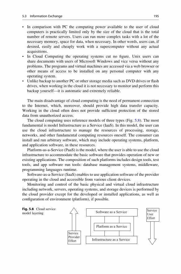
• In comparison with PC the computing power available to the user of cloud
computers is practically limited only by the size of the cloud that is the total
number of remote servers. Users can run more complex tasks with a lot of the
necessary memory, space for data, when necessary. In other words, users can, if
desired, easily and cheaply work with a supercomputer without any actual
acquisitions.
• In Cloud Computing the operating systems cut no figure. Unix users can
share documents with users of Microsoft Windows and vice versa without any
problems. The programs and virtual machines are accessed via a web browser or
other means of access to be installed on any personal computer with any
operating system.
• Unlike backup to another PC or other storage media such as DVD drives or flash
drives, when working in the cloud it is not necessary to monitor and perform this
backup yourself—it is automatic and extremely reliable.
The main disadvantage of cloud computing is the need of permanent connection
to the Internet, which, moreover, should provide high data transfer capacity.
Working in the cloud often does not provide sufficient protection of the stored
data from unauthorized access.
The cloud computing uses reference models of three types (Fig. 5.8). The most
fundamental is model Infrastructure as a Service (IaaS). In this model, the user can
use the cloud infrastructure to manage the resources of processing, storage,
networks, and other fundamental computing resources oneself. The consumer can
install and run arbitrary software, which may include operating systems, platform,
and application software, in these resources.
Platform-as-a-Service (PaaS) is the model, where the user is able to use the cloud
infrastructure to accommodate the basic software that provides operation of new or
existing applications. The composition of such platforms includes design tools, test
tools, and app software run tools: database management systems, middleware,
programming languages runtime.
Software-as-a-Service (SaaS) enables to use application software of the provider
operating in the cloud and accessible from various client devices.
Monitoring and control of the basic physical and virtual cloud infrastructure
including network, servers, operating systems, and storage devices is performed by
the cloud provider except for the developed or installed applications, as well as
configuration of environment (platform), if possible.
Infrastructure as a Service
Platform as a Service
Software as a Service
Service ProviderEffort
Service UserEffort
Fig. 5.8 Cloud service
model layering
5.3 Information Exchange 195
As follows from Fig. 5.8, higher layering of the use of cloud models requires
more efforts of the cloud provider but the work of users becomes easier at the same
time. On the contrary, lower layering of the model leads to lower requirements for
the provider, but the user’s work becomes more complicated.
From the point of view of the users of information systems for production
planning, the work with such a system in the cloud is extremely useful when
selecting the system to be most suitable for a particular company. In this case,
without investing heavily in purchasing the system, the customer can work with it
on lease for the time enough to explore it properly.
If the decision is made on implementation of the system at the enterprise, then
the practicability of further work in the cloud depends on the scale of the enterprise.
If the scale is significant, it makes sense to gradually abandon the cloud services
provider, as the computational capabilities of the enterprise increase. For small
businesses, the work in the cloud is probably the only opportunity to use modern
powerful information systems. An example of operation in the cloud with one of
such systems is shown in Appendix F.
References
Alperovich, M. (2001). Introduction to OLAP and multidimensional databases. www.olap.ru(in Russian).
APICS Dictionary. (2008). American Production and Inventory Control Society (12th ed.). www.
apics.org
Biennier, F., Ali, L., & Legait, A. (2007). Extended service integration: Towards “manufacturing”
SLA. In IFIP International federation for information processing. Advances in productionmanagement systems (pp. 87–94). Boston: Springer.
Cassina, J., Tomasella, M., Matta, A., & Taisch, M. (2007). Closed-loop PLM of household
appliances: An industrial approach. In IFIP International federation for informationprocessing. Advances in production management systems (pp. 153–160). Boston: Springer.
Dreyer, H., Bakas, O., Alfnes, E., Strandhagen, O., & Kollberg, M. (2007). Global supply chain
control: A conceptual framework for the global control centre. In IFIP International federationfor information processing. Advances in production management systems (pp. 161–170).
Boston: Springer.
Etgar, M. (2008). A descriptive model of the consumer co-production process. Journal of theAcademy of Marketing Science, 36, 97–108.
Grachiova, K. A., Zakharova, M. K., Odintsova, L. A., Stepanov, V. V., Pickunova, C. A.,
Smolyankin, G. V., et al. (2005). In Y. V. Skvortsov & L. A. Nekrasov (Eds.), Managementand planning of machinery production. Moscow: Vysshaya Shkola (in Russian).
Hinkelmann, K., Meyer, M., & Schmalhofer, F. (1994). Knowledge-base evolution for product and
production planning. AICOM, 7, 98–113.Huang, G. Q., Lau, S. K., & Mak, K. L. (2003). The impact of sharing production information on
supply chain dynamics: A review of the literature. www.imse.hku.hk/. . .Survey.htmKargin, A. A., & Mironenko, D. S. (2008). Experience in automation of production planning at
OJSC MZTM. www.nbuv.gov.ua/portal/Natura. . .Kargin.pdf (in Russian).
Lele, M. (1997). After-sales service-necessary evil or strategic opportunity. Managing ServiceQuality, 7, 141–145.
NIST Special Publication (SP) 800-145. A NIST definition of cloud computing. csrc.nist.gov/publications/. . ./SP800-145.pdf
196 5 Data for Planning

Novitsky, O. V. (2010). Production planning system with the use of analytical models bank.
Information-Management Systems, 3, 75–79 (in Russian).
Osadsky, P., Garg, A., Nitu, B., Schneider, O., & Schleyer, S. (2007). Improving service operation
performance by a cross-industry reference model. In IFIP International federation for infor-mation processing. Advances in production management systems (pp. 397–404). Boston:
Springer.
Shapiro, J. F. (2001). Modelling the supply chain. Pacific Grove, CA: Thomson Learning.
Smirnov, O. (2004). What is knowledge base and what is it for. www.bigc.ru (in Russian).
Stadtler, H., & Kilger, C. (2008). Supply chain management and advanced planning. Concepts,models, software, and case studies (4th ed.). Berlin: Springer.
Tsumaya, A., Matoba, Y., Wakamatsu, H., & Arai, E. (2007). Dynamic management architecture
for project based production. In IFIP International federation for information processing.Advances in production management systems (pp. 229–236). Boston: Springer.
Wailgum, T. (2008). Supply chain management definition and solutions. www.cio.comYamaji, M., & Amasaka, K. (2007). Proposal and validity of global intelligence partnering model
of corporate strategy, GIPM-CS. In IFIP International federation for information processing.Advances in production management systems (pp. 59–67). Boston: Springer.
Zaratuychenko, О. (1998). Modern approaches and methods to develop analytical informationsystems. www.bis.ru/pr (in Russian).
Zhu, Y. M., Alard, R., & Schoensleben, P. (2007). Design quality: A key factor to improve the
product quality in international production network. In IFIP International federation forinformation processing. Advances in production management systems (pp. 133–141). Boston:Springer.
References 197
Demand Forecasting 6
6.1 Demand Modelling Based on Time Series Analysis
Routine observation of the product quantity demanded results in recording a time-
ordered sequence of values of this demand. This sequence is called a time series.
Usually, observations are performed at regular intervals and numbered sequentially.
As the demand values vary randomly then the corresponding time series is a
random variable. The main purpose of the time series study is to forecast, i.e. to
make an attempt to predict the future values of the time series based on its present
and past values.
Numerous observations of different time series show that the current value of
random variable in question D at time t is dependent on four factors
Dt ¼ f It; bt;Ct; etð Þ; ð6:1Þwhere It is the so-called seasonality index reflecting the seasonal effect; bt is thetrend, i.e. systematic motion; Ct is more or less regular fluctuations against trend;
and et is the random value.
In the simplest case demand D is the value falling under random deviations from
a certain constant value a, i.e.
Dt ¼ aþ et: ð6:2ÞDependence (Eq. 6.2) describes the demand for the products on the market in
stable development stage described above in Sect. 1.6.1. The example of these
products can be toothpastes, spare parts, some tools, etc.
If a product belongs to any other market quadrant shown above in Fig. 1.10, then
the demand for the product increases (new or growing market) or decreases (mature
market). In this case, the demand, for the most part, can be approximately described
by the following dependence:
# Springer International Publishing Switzerland 2016
Y. Mauergauz, Advanced Planning and Scheduling in Manufacturing and SupplyChains, DOI 10.1007/978-3-319-27523-9_6
199
Dt ¼ aþ btþ et; ð6:3Þwhere b is the trend coefficient, which can be either positive or negative.
Taking into account the seasonality index, expression (6.3) can be written as
Dt ¼ aþ btð ÞIt þ et; ð6:4Þreflecting the so-called multiplicative seasonality model. In terms of this model it is
assumed that if 1 year includes T of various seasonal periods, then for any of these
subsequent periods the following expression is valid:
XTk¼1
Itþk ¼ T; ð6:5Þ
i.e. the average seasonality index is equal to 1.
With multiplicative seasonality, the value of seasonal fluctuations depends
on the overall level of the time series values. Unlike this type of seasonality, the
so-called additive seasonality can be observed, where the demand of the form
(Eq. 6.2) is added with some periodic component with period l, i.e.
Dt ¼ aþ It þ et; ð6:6Þand the following condition is observed:
It ¼ Itþl: ð6:7ÞAn example of multiplicative seasonality can be the market of toys, sales of
which are growing in the pre-holiday period. The more popular toy in ordinary days
is, the more the demand for it grows during holidays. The additive seasonality is
true for the goods, consumption of which is concentrated in certain periods and
depends little on the consumption in other periods. These products include, for
example, ice cream, soft drinks, fur products, etc.
The use of more complex models of time series does not necessarily lead to
better results in forecasting (Axseter 2006). The reason for this is the significant
influence of random component et in the above dependencies. With large scatter of
et the simpler models can lead to even better results than more complex ones.
Any forecast is usually prepared in advance for several specific forecast periods.
The time interval, for which the forecast is prepared, is called a forecast interval.
The number of the periods, for which a one-time forecast is made, is a forecasting
horizon. For example, if the forecast interval is 1 month, the forecasting horizon is
three, and if the forecast is made at the end of December, the forecast period is
January, February, and March of the next year.
At the end of forecast period t, for each forecast it is possible to define its
deviation value Mt from the actual demand value for this period, which can be
evaluated more conveniently in percentage of the actual demand
200 6 Demand Forecasting
Mt ¼ 100D
0t � Dt
Dt%; ð6:8Þ
where D0t is the forecast value and Dt is the actual demand value.
The quality of forecasting is determined by two main indices—mean forecast
error for n periods
M ¼ 100
Xnt¼1
D0t � Dt
� �=Dt
n% ð6:9Þ
and mean absolute forecast error
Ma ¼ 100
Xnt¼1
��D0t � Dt
��=Dt
n%: ð6:10Þ
Assume that in April it appears that forecast errors for January, February, and
March have made �20 %, +15 % and �7 %, accordingly. In this case M ¼ �4%
and Ma ¼ �14%. Mean absolute forecast error Ma describes the range of possible
deviations from the demand while mean error M defines how much the forecast
trend itself deviates from the demand trend.
6.2 Main Methods of Forecasting
All of the following methods are based on the use of historical data on supply and
extrapolate the found tendencies of the demand to a relatively small forecasting
horizon (up to a year).
6.2.1 Moving Average Method
In the cases where the available time series data due to the large random or periodic
fluctuations make it difficult to identify the process trend, it is possible to use the
moving-average method to determine the trend. This method involves the replace-
ment of the actual time series values with the calculated values, which have much
smaller fluctuations than the original. In this method, we calculate average values of
the variable data based on groups of data for a certain period of time, and each
subsequent group shifts against the previous one by one period (month, year, etc.).
When forecasting, it is assumed that the demand value in the coming accounting
period will be equal to the average demand calculated for the last time interval
elapsed.
6.2 Main Methods of Forecasting 201
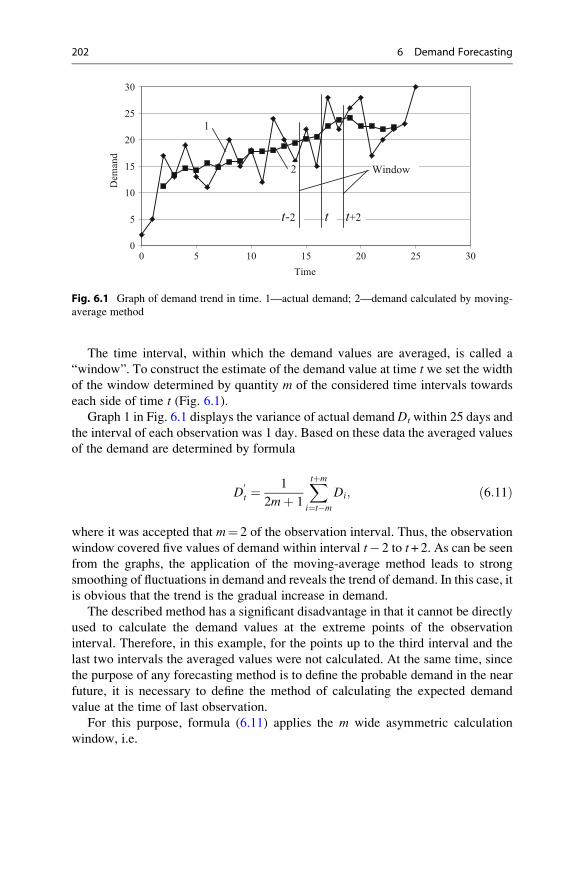
The time interval, within which the demand values are averaged, is called a
“window”. To construct the estimate of the demand value at time t we set the widthof the window determined by quantity m of the considered time intervals towards
each side of time t (Fig. 6.1).Graph 1 in Fig. 6.1 displays the variance of actual demand Dt within 25 days and
the interval of each observation was 1 day. Based on these data the averaged values
of the demand are determined by formula
D0t ¼
1
2mþ 1
Xtþm
i¼t�m
Di; ð6:11Þ
where it was accepted that m¼ 2 of the observation interval. Thus, the observation
window covered five values of demand within interval t� 2 to t+ 2. As can be seenfrom the graphs, the application of the moving-average method leads to strong
smoothing of fluctuations in demand and reveals the trend of demand. In this case, it
is obvious that the trend is the gradual increase in demand.
The described method has a significant disadvantage in that it cannot be directly
used to calculate the demand values at the extreme points of the observation
interval. Therefore, in this example, for the points up to the third interval and the
last two intervals the averaged values were not calculated. At the same time, since
the purpose of any forecasting method is to define the probable demand in the near
future, it is necessary to define the method of calculating the expected demand
value at the time of last observation.
For this purpose, formula (6.11) applies the m wide asymmetric calculation
window, i.e.
0
5
10
15
20
25
30
0 5 10 15 20 25 30
Dem
and
Time
t+2t-2
1
2
t
Window
Fig. 6.1 Graph of demand trend in time. 1—actual demand; 2—demand calculated by moving-
average method
202 6 Demand Forecasting

D0tþ1 ¼
1
mþ 1
Xti¼t�m
Di: ð6:12Þ
For example, in this case, with m¼ 4 and t¼ 25
D026 ¼
D21 þ D22 þ D23 þ D24 þ D25ð Þ4þ 1
¼ 22:4:
6.2.2 Exponentially Smoothing Forecasting
In forecasting, the influence of actual demand data on the forecast value should
obviously decrease with increasing distance of the data from the current time.
One of simple but widely used methods that take into account this data “ageing”
is the method of exponential smoothing. In this method, exponential averageD0tþ1 is
constructed similarly to asymmetric moving average, but takes into account the
data ageing degree. Moreover, each new forecast is based on the account of the
previous forecast and its deviation from the actual value, namely
D0tþ1 ¼ αDt þ 1� αð ÞD0
t, 0 � α � 1; ð6:13Þwhere α is the smoothing parameter defining the weight of the last actual observa-
tion Dt when preparing the forecast for the next time interval. The more influence
the last observed value has in the forecasting model, the higher parameter α should
be selected.
Value D0t in expression (6.13) is the value of estimated forecast, which is made at
the previous stage. Therefore, to use formula (6.13), it is necessary to find value D0t
at some initial point of calculation. Usually, in capacity of this initial value D0t the
actual demand value at the first point of the period in question is taken.
For example, pursuant to the graph of actual demand in Fig. 6.1, at time t¼ 0
D00 ¼ D0 ¼ 2. Then
D01 ¼ 0:3D0 þ 1� 0:3ð ÞD0
0 ¼ 2;
D02 ¼ 0:3D1 þ 1� 0:3ð ÞD0
1 ¼ 2:9;::::
D026 ¼ 0:3D25 þ 1� 0:3ð ÞD0
25 ¼ 24:4:
Figure 6.2 presents the graph of actual variation of the demand coinciding with
the graph in Fig. 6.1, as well as two graphs built by formula (6.13) with two
different values of α.From the graphs in Fig. 6.2, it is clear that the forecast for time t¼ 26 according
to the exponential smoothing method with α ¼ 0:3 is 24.4, while with α ¼ 0:6 is
26.9. Both of these forecasts have error probability, which can be estimated by
6.2 Main Methods of Forecasting 203
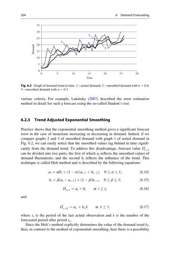
various criteria. For example, Lukinsky (2007) described the error estimation
method in detail for such a forecast using the so-called Student’s test.
6.2.3 Trend Adjusted Exponential Smoothing
Practice shows that the exponential smoothing method gives a significant forecast
error in the case of monotone increasing or decreasing in demand. Indeed, if we
compare graphs 2 and 3 of smoothed demand with graph 1 of actual demand in
Fig. 6.2, we can easily notice that the smoothed values lag behind in time signifi-
cantly from the demand trend. To address this disadvantage, forecast value D0tþ1
can be divided into two parts, the first of which at reflects the smoothed values of
demand fluctuations, and the second bt reflects the influence of the trend. This
technique is called Holt method and is described by the following equations:
at ¼ αDt þ 1� αð Þ at�1 þ bt�1ð Þ, 0 � α � 1; ð6:14Þbt ¼ β at � at�1ð Þ þ 1� βð Þbt�1, 0 � β � 1; ð6:15Þ
D0tþ1 ¼ at þ bt at t � te ð6:16Þ
and
D0teþk ¼ ate þ btek at k � 1; ð6:17Þ
where te is the period of the last actual observation and k is the number of the
forecasted period after period te.Since the Holt’s method explicitly determines the value of the demand trend bt,
then, in contrast to the method of exponential smoothing, here there is a possibility
0
5
10
15
20
25
30
35
0 5 10 15 20 25 30
Dem
and
Time
1
2
3
Fig. 6.2 Graph of demand trend in time. 1—actual demand; 2—smoothed demand with α ¼ 0:6;3—smoothed demand with α ¼ 0:3
204 6 Demand Forecasting
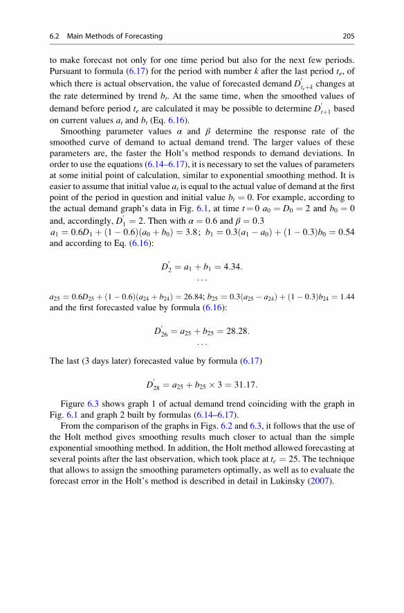
to make forecast not only for one time period but also for the next few periods.
Pursuant to formula (6.17) for the period with number k after the last period te, of
which there is actual observation, the value of forecasted demand D0teþk changes at
the rate determined by trend bt. At the same time, when the smoothed values of
demand before period te are calculated it may be possible to determine D0tþ1 based
on current values at and bt (Eq. 6.16).Smoothing parameter values α and β determine the response rate of the
smoothed curve of demand to actual demand trend. The larger values of these
parameters are, the faster the Holt’s method responds to demand deviations. In
order to use the equations (6.14–6.17), it is necessary to set the values of parameters
at some initial point of calculation, similar to exponential smoothing method. It is
easier to assume that initial value at is equal to the actual value of demand at the first
point of the period in question and initial value bt ¼ 0. For example, according to
the actual demand graph’s data in Fig. 6.1, at time t¼ 0 a0 ¼ D0 ¼ 2 and b0 ¼ 0
and, accordingly, D01 ¼ 2. Then with α ¼ 0:6 and β ¼ 0:3
a1 ¼ 0:6D1 þ 1� 0:6ð Þ a0 þ b0ð Þ ¼ 3:8; b1 ¼ 0:3 a1 � a0ð Þ þ 1� 0:3ð Þb0 ¼ 0:54and according to Eq. (6.16):
D02 ¼ a1 þ b1 ¼ 4:34:
. . .
a25 ¼ 0:6D25 þ 1� 0:6ð Þ a24 þ b24ð Þ ¼ 26:84; b25 ¼ 0:3 a25 � a24ð Þ þ 1� 0:3ð Þb24 ¼ 1:44
and the first forecasted value by formula (6.16):
D026 ¼ a25 þ b25 ¼ 28:28:
. . .
The last (3 days later) forecasted value by formula (6.17)
D028 ¼ a25 þ b25 � 3 ¼ 31:17:
Figure 6.3 shows graph 1 of actual demand trend coinciding with the graph in
Fig. 6.1 and graph 2 built by formulas (6.14–6.17).
From the comparison of the graphs in Figs. 6.2 and 6.3, it follows that the use of
the Holt method gives smoothing results much closer to actual than the simple
exponential smoothing method. In addition, the Holt method allowed forecasting at
several points after the last observation, which took place at te ¼ 25. The technique
that allows to assign the smoothing parameters optimally, as well as to evaluate the
forecast error in the Holt’s method is described in detail in Lukinsky (2007).
6.2 Main Methods of Forecasting 205
6.2.4 Trend and Seasonality Adjusted Exponential Smoothing
If actual data of demand observations reveal systematic fluctuations of the demand,
then they indicate the presence of a seasonal component. The annual fluctuations
with 12-month observation period repeat most often. Weekly fluctuations are also
frequent. They give peaks of demand, such as on weekends.
In the examples of Figs. 6.1–6.3 regular fluctuations with period l equallingabout 5 days of observation can be noticed. We assume that in capacity of
observation days here only weekdays are used. In this case, we can believe that
the demand curve here has a weekly seasonality with the peak falling within the
middle of the week.
The most common method of forecasting taking into account the trend and
seasonality is now considered to the method that uses the so-called the Winters
model. The Winters model actually expands the Holt method to the case when there
is seasonality. For this purpose, besides parameters α and β the third smoothing
parameter γ is introduced in addition, and accordingly the amount of calculation
equations increases:
at ¼ αDt
It�lþ 1� αð Þ at�1 þ bt�1ð Þ, 0 � α � 1; ð6:18Þ
bt ¼ β at � at�1ð Þ þ 1� βð Þbt�1, 0 � β � 1; ð6:19ÞIt ¼ I0 at t < l ð6:20Þ
and
0
5
10
15
20
25
30
35
0 5 10 15 20 25 30
Dem
and
Time
1
2
Fig. 6.3 Graph of demand trend in time. 1—actual demand; 2—demand calculated by the Holt’s
method
206 6 Demand Forecasting
It ¼ γDt
atþ 1� γð ÞIt�l at t � l, 0 � γ � 1; ð6:21Þ
D0tþ1 ¼ at þ btð ÞIt�l at t � te ð6:22Þ
and
D0teþk ¼ ate þ btekð ÞIte�lþk at k � 1: ð6:23Þ
To calculate, similarly to the previous paragraph, we assume that initial value atis equal to the demand value at the first point of the period in question, and initial
valuebt ¼ 0, i.e. in accordance with the data of the actual demand in Fig. 6.1 at time
t¼ 0 a0 ¼ D0 ¼ 2 and b0 ¼ 0. Besides, we assume that initial value of seasonality
index I0 ¼ 1 and accordingly from Eq. (6.22) we obtain D01 ¼ 2.
Further with α ¼ 0:6, β ¼ 0:4 and γ ¼ 0:3 we have
a1 ¼ 0:6D1
1þ 1� 0:6ð Þ a0 þ b0ð Þ ¼ 3:8; b1 ¼ 0:4 a1 � a0ð Þ þ 1� 0:4ð Þb0 ¼ 0:72:
Pursuant to Eq. (6.20) the first value I1 ¼ 1 and smoothed demand value
D02 ¼ a1 þ b1ð ÞI0 ¼ 4:52
. . .
a25 ¼ 0:6D25
I20þ 1� 0:6ð Þ a24 þ b24ð Þ ¼ 25:42;
b25 ¼ 0:4 a25 � a24ð Þ þ 1� 0:4ð Þb24 ¼ 1:85;
I25 ¼ 0:3D25
a25þ 1� 0:3ð ÞI20 ¼ 1:09 and first forecasted value according to
Eq. (6.22):
D026 ¼ a25 þ b25ð ÞI20 ¼ 27:06:
. . .
The last (3 days later) forecasted value of demand in accordance with Eq. (6.23):
D028 ¼ a25 þ b25 � 3ð ÞI23 ¼ 31:9:
Figure 6.4 shows graph 1 of actual demand trend coinciding with the graph in
Fig. 6.1, and graph 2, built by formulas (6.18–6.23).
Let us compare the graphs in Figs. 6.2–6.4. In this case, it turns out that the
Winters method gives smoothing results quite close to the original actual data. It
follows that the probability of correct forecast can increase significantly.
In the paper of Makridakis and Hibon (2000), the quality of forecasting for
21 different models was studied, and forecasts were tested on approximately 1000
time series. The results showed clearly that the use of more complex models has
6.2 Main Methods of Forecasting 207
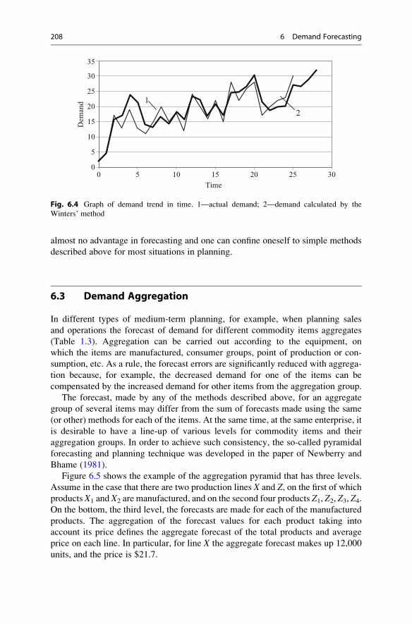
almost no advantage in forecasting and one can confine oneself to simple methods
described above for most situations in planning.
6.3 Demand Aggregation
In different types of medium-term planning, for example, when planning sales
and operations the forecast of demand for different commodity items aggregates
(Table 1.3). Aggregation can be carried out according to the equipment, on
which the items are manufactured, consumer groups, point of production or con-
sumption, etc. As a rule, the forecast errors are significantly reduced with aggrega-
tion because, for example, the decreased demand for one of the items can be
compensated by the increased demand for other items from the aggregation group.
The forecast, made by any of the methods described above, for an aggregate
group of several items may differ from the sum of forecasts made using the same
(or other) methods for each of the items. At the same time, at the same enterprise, it
is desirable to have a line-up of various levels for commodity items and their
aggregation groups. In order to achieve such consistency, the so-called pyramidal
forecasting and planning technique was developed in the paper of Newberry and
Bhame (1981).
Figure 6.5 shows the example of the aggregation pyramid that has three levels.
Assume in the case that there are two production lines X and Z, on the first of whichproducts X1 and X2 are manufactured, and on the second four products Z1, Z2, Z3, Z4.On the bottom, the third level, the forecasts are made for each of the manufactured
products. The aggregation of the forecast values for each product taking into
account its price defines the aggregate forecast of the total products and average
price on each line. In particular, for line X the aggregate forecast makes up 12,000
units, and the price is $21.7.
0
5
10
15
20
25
30
35
0 5 10 15 20 25 30
Dem
and
Time
1
2
Fig. 6.4 Graph of demand trend in time. 1—actual demand; 2—demand calculated by the
Winters’ method
208 6 Demand Forecasting
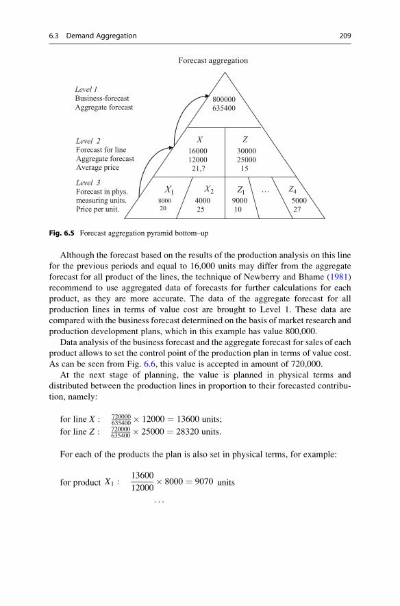
Although the forecast based on the results of the production analysis on this line
for the previous periods and equal to 16,000 units may differ from the aggregate
forecast for all product of the lines, the technique of Newberry and Bhame (1981)
recommend to use aggregated data of forecasts for further calculations for each
product, as they are more accurate. The data of the aggregate forecast for all
production lines in terms of value cost are brought to Level 1. These data are
compared with the business forecast determined on the basis of market research and
production development plans, which in this example has value 800,000.
Data analysis of the business forecast and the aggregate forecast for sales of each
product allows to set the control point of the production plan in terms of value cost.
As can be seen from Fig. 6.6, this value is accepted in amount of 720,000.
At the next stage of planning, the value is planned in physical terms and
distributed between the production lines in proportion to their forecasted contribu-
tion, namely:
for line X : 720000635400
� 12000 ¼ 13600 units;
for line Z : 720000635400
� 25000 ¼ 28320 units.
For each of the products the plan is also set in physical terms, for example:
for product X1 :13600
12000� 8000 ¼ 9070
. . .
units
Level 3 Forecast in phys. measuring units.Price per unit.
1X 2X1Z 4Z…
X Z
Level 1Business-forecastAggregate forecast
800020
400025
900010
1600012000
21,7
3000025000
15
500027
800000635400
Forecast aggregation
Level 2 Forecast for lineAggregate forecastAverage price
Fig. 6.5 Forecast aggregation pyramid bottom–up
6.3 Demand Aggregation 209
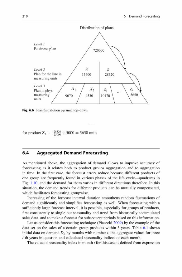
. . .
for product Z4 :2832025000
� 5000 ¼ 5650 units
6.4 Aggregated Demand Forecasting
As mentioned above, the aggregation of demand allows to improve accuracy of
forecasting as it relates both to product groups aggregation and to aggregation
in time. In the first case, the forecast errors reduce because different products of
one group are frequently found in various phases of the life cycle—quadrants in
Fig. 1.10, and the demand for them varies in different directions therefore. In this
situation, the demand trends for different products can be mutually compensated,
which facilitates forecasting groupwise.
Increasing of the forecast interval duration smoothens random fluctuations of
demand significantly and simplifies forecasting as well. When forecasting with a
sufficiently large forecast interval, it is possible, especially for groups of products,
first consistently to single out seasonality and trend from historically accumulated
sales data, and to make a forecast for subsequent periods based on this information.
Let us consider this forecasting technique (Piasecki 2009) by the example of the
data set on the sales of a certain group products within 3 years. Table 6.1 shows
initial data on demand Dti by months with number t, the aggregate values for threei-th years in question and calculated seasonality indices of each month.
The value of seasonality index in month t for this case is defined from expression
1X2X
1Z 4Z…
X Z
Distribution of plans
720000
Level 1Business plan
Level 2Plan for the line in measuring units
Level 3Plan in phys. measuring units.
13600 28320
9070 4530 10170 5650
Fig. 6.6 Plan distribution pyramid top–down
210 6 Demand Forecasting
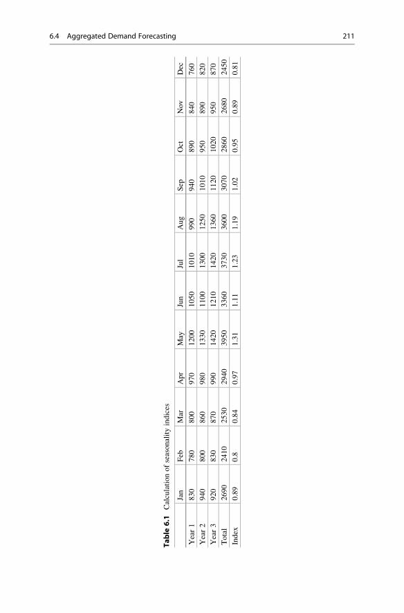
Table
6.1
Calculationofseasonalityindices
Jan
Feb
Mar
Apr
May
Jun
Jul
Aug
Sep
Oct
Nov
Dec
Year1
830
780
800
970
1200
1050
1010
990
940
890
840
760
Year2
940
800
860
980
1330
1100
1300
1250
1010
950
890
820
Year3
920
830
870
990
1420
1210
1420
1360
1120
1020
950
870
Total
2690
2410
2530
2940
3950
3360
3730
3600
3070
2860
2680
2450
Index
0.89
0.8
0.84
0.97
1.31
1.11
1.23
1.19
1.02
0.95
0.89
0.81
6.4 Aggregated Demand Forecasting 211
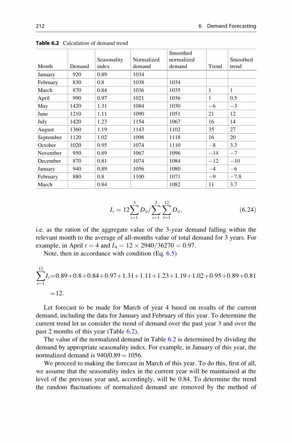
It ¼ 12X3i¼1
Dti=X3i¼1
X12t¼1
Dti; ð6:24Þ
i.e. as the ration of the aggregate value of the 3-year demand falling within the
relevant month to the average of all-months value of total demand for 3 years. For
example, in April t ¼ 4 and I4 ¼ 12� 2940=36270 ¼ 0:97.Note, then in accordance with condition (Eq. 6.5)
X12t¼1
It¼0:89þ0:8þ0:84þ0:97þ1:31þ1:11þ1:23þ1:19þ1:02þ0:95þ0:89þ0:81
¼12:
Let forecast to be made for March of year 4 based on results of the current
demand, including the data for January and February of this year. To determine the
current trend let us consider the trend of demand over the past year 3 and over the
past 2 months of this year (Table 6.2).
The value of the normalized demand in Table 6.2 is determined by dividing the
demand by appropriate seasonality index. For example, in January of this year, the
normalized demand is 940/0.89¼ 1056.
We proceed to making the forecast in March of this year. To do this, first of all,
we assume that the seasonality index in the current year will be maintained at the
level of the previous year and, accordingly, will be 0.84. To determine the trend
the random fluctuations of normalized demand are removed by the method of
Table 6.2 Calculation of demand trend
Month Demand
Seasonality
index
Normalized
demand
Smoothed
normalized
demand Trend
Smoothed
trend
January 920 0.89 1034
February 830 0.8 1038 1034
March 870 0.84 1036 1035 1 1
April 990 0.97 1021 1036 1 0.5
May 1420 1.31 1084 1030 �6 �3
June 1210 1.11 1090 1051 21 12
July 1420 1.23 1154 1067 16 14
August 1360 1.19 1143 1102 35 27
September 1120 1.02 1098 1118 16 20
October 1020 0.95 1074 1110 �8 3.3
November 950 0.89 1067 1096 �14 �7
December 870 0.81 1074 1084 �12 �10
January 940 0.89 1056 1080 �4 �6
February 880 0.8 1100 1071 �9 �7.8
March 0.84 1082 11 3.7
212 6 Demand Forecasting
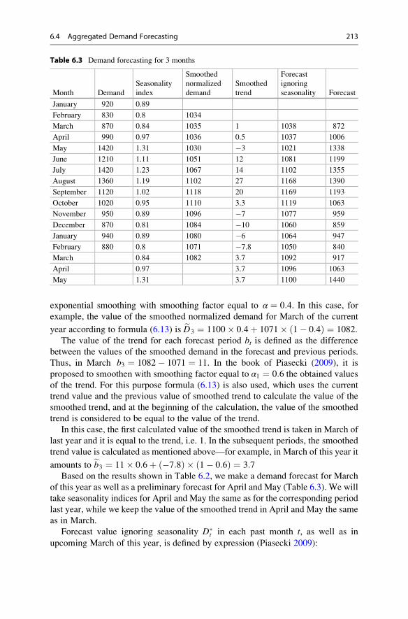
exponential smoothing with smoothing factor equal to α ¼ 0:4. In this case, for
example, the value of the smoothed normalized demand for March of the current
year according to formula (6.13) is eD3 ¼ 1100� 0:4þ 1071� 1� 0:4ð Þ ¼ 1082.
The value of the trend for each forecast period bt is defined as the difference
between the values of the smoothed demand in the forecast and previous periods.
Thus, in March b3 ¼ 1082� 1071 ¼ 11. In the book of Piasecki (2009), it is
proposed to smoothen with smoothing factor equal to α1 ¼ 0:6 the obtained values
of the trend. For this purpose formula (6.13) is also used, which uses the current
trend value and the previous value of smoothed trend to calculate the value of the
smoothed trend, and at the beginning of the calculation, the value of the smoothed
trend is considered to be equal to the value of the trend.
In this case, the first calculated value of the smoothed trend is taken in March of
last year and it is equal to the trend, i.e. 1. In the subsequent periods, the smoothed
trend value is calculated as mentioned above—for example, in March of this year it
amounts to eb3 ¼ 11� 0:6þ �7:8ð Þ � 1� 0:6ð Þ ¼ 3:7Based on the results shown in Table 6.2, we make a demand forecast for March
of this year as well as a preliminary forecast for April and May (Table 6.3). We will
take seasonality indices for April and May the same as for the corresponding period
last year, while we keep the value of the smoothed trend in April and May the same
as in March.
Forecast value ignoring seasonality Dt in each past month t, as well as in
upcoming March of this year, is defined by expression (Piasecki 2009):
Table 6.3 Demand forecasting for 3 months
Month Demand
Seasonality
index
Smoothed
normalized
demand
Smoothed
trend
Forecast
ignoring
seasonality Forecast
January 920 0.89
February 830 0.8 1034
March 870 0.84 1035 1 1038 872
April 990 0.97 1036 0.5 1037 1006
May 1420 1.31 1030 �3 1021 1338
June 1210 1.11 1051 12 1081 1199
July 1420 1.23 1067 14 1102 1355
August 1360 1.19 1102 27 1168 1390
September 1120 1.02 1118 20 1169 1193
October 1020 0.95 1110 3.3 1119 1063
November 950 0.89 1096 �7 1077 959
December 870 0.81 1084 �10 1060 859
January 940 0.89 1080 �6 1064 947
February 880 0.8 1071 �7.8 1050 840
March 0.84 1082 3.7 1092 917
April 0.97 3.7 1096 1063
May 1.31 3.7 1100 1440
6.4 Aggregated Demand Forecasting 213

D*t ¼ eDt þ ebt=α; ð6:25Þ
and the total seasonality-adjusted forecast is
D0t ¼ D*
t It; ð6:26Þ
where eDt as above is the smoothed normalized demand, ebt is the smoothed trend, Itis the seasonality index, and α is the smoothing coefficient of normalized demand.
In this case for March of this year, we haveD*3 ¼ 1082þ 3:7=0:4 ¼ 1092 and total
forecast value D03 ¼ 1092� 0:84 ¼ 917.
For an approximate forecast for the subsequent months, it is proposed in Piasecki
(2009) to define a new forecast without taking into account seasonality by simply
adding the trend, namely:
D*t ¼ D*
t�1 þ ebt: ð6:27Þ
For example, for April we will obtain D*4 ¼ 1092þ 3:7 � 1096 and the total
seasonality-adjusted forecast is D04 ¼ 1096� 0:97 ¼ 1063.
References
Axseter, S. (2006). Inventory control. Berlin: Springer.Lukinsky, V. S. (2007). Models and methods of logistics. Saint Petersburg: Piter (in Russian).
Makridakis, S., & Hibon, M. (2000). M3 competition: Results, conclusion and implications.
International Journal of Forecasting, 16, 451–476.Newberry, T. L., & Bhame, C. D. (1981). How management should use and interact with sales
forecast. Inventories and Production Magazine, 1(3), 1–13.Piasecki, D. J. (2009). Inventory management explained. Pleasant Prairie: Ops Publishing.
214 6 Demand Forecasting
Examples of Advanced Planning Models 7
7.1 Joint Operation Model of APS System and ERP Systemfrom SAP R/3
The main joint operation of various APS systems and R/3 system is the diagram of
Stadtler and Kilger (2008) shown in Fig. 7.1. This diagram reflects planning tasks
in supply chains (SC) and has the form of so-called Operations—Time horizons
matrix.
Pursuant to Fig. 7.1 planning modules shall provide elaboration of long-term
tasks, mid-term tasks and short-term schedules for the four operations—procure-
ment, production, distribution, and sales. It is necessary to note the difference in
understanding the master planning in the diagram in Fig. 7.1 and the common
notion of master plan in ERP systems. In fact, the master planning in Fig. 7.1 refers
to development of sales and operations plan of ERP systems (Table 1.3). Accord-
ingly, the notion of production planning in Fig. 7.1 is equivalent to the master
plan and the material requirement plan in the ERP system, and the scheduling is
equivalent to operational planning.
This matrix does not show directly which components of the planning should be
performed within the ERP system and which should be assigned to the APS system
or any other system. As a rule, the developers of various APS systems select some
part from this diagram, develop the software for it and interface it with the basic
ERP system. In this case, it is inevitable that there is duplication of functions from
one side and planning objectives may be unachieved from the other side.
Typically, APS systems of this type are designed to work with SAP R/3 system.
The considerable experience of joint operation of such complex systems in various
industries has led to the widely spread belief that it is this way of advanced planning
that is at least the core way, if not essential.
Above in Sect. 1.4, the place of advanced planning in the enterprise information
system was discussed in detail, from which it follows that the modern planning can
be applied in a variety of options including the model considered in this section.
The reason for this widespread application of this method, in our opinion, is that the
# Springer International Publishing Switzerland 2016
Y. Mauergauz, Advanced Planning and Scheduling in Manufacturing and SupplyChains, DOI 10.1007/978-3-319-27523-9_7
215
developers need to apply the new methods of planning somehow without significant
modifications in the old ERP systems. Let us consider three examples of imple-
mentation of such models.
7.1.1 Main Business Process Attributes in Various Industries
Earlier in Sect. 1.2.1, it was noted that every business process of SC could be
characterized by a set of functional and structural attributes. Table 7.1 shows the
values of the functional attributes for enterprises of three different industries
(Stadtler and Kilger 2008).
Comparison of the functional attributes of enterprises in Table 7.1 reveals
significant differences in the nature of their activities. First of all, it refers to the
nomenclature (attribute 1) and shelf life of incoming materials and components
(attribute 3). The computer build company uses a much larger nomenclature of
incoming components than the other two companies do in Table 7.1, and at the
same time, the shelf life of these components is much shorter.
In addition, the computer build company is much more dependent on customers.
Indeed, the dispatch (attribute 9) in this case is performed when the orders are
processed, and thus the production lot size (attribute 5) can vary. Besides, there is
an opportunity here to vary products’ configuration according to the customer’s
special requirements (attribute 15). As a result, the life cycle of products of this
company (attribute 13) is much shorter than for other comparable companies.
The computer build company has the configurable flow-line production (attri-
bute 4) of type 3b (Sect. 1.2.1), focused on the production of core products. In
addition, the individual computer units are assembled at cell manufacturing sites
Procurement Production Distribution Sales
Strategic network planningLong-term
Master planningMid-term
Purchasing and material
requirements
planningShort-term
Production
planning
Scheduling
Distribution
planning
Transport planning
Demand
planning
Demand fulfilment and ATP
Planning:
Operations:
Fig. 7.1 Planning modules for SC matrix [based on Stadtler and Kilger (2008)]
216 7 Examples of Advanced Planning Models

(type 4). The other two companies operate with configurable flow-line production
of type 3c, where it is possible to produce by-products in parallel with the core
products. This is a large-lot production (Table 1.2), i.e. it has a quite large scale.
With these scales, the optimization of Sales and Operations Plan by the maxi-
mum profit criterion (Sect. 2.2.3) is of prime importance. In addition, at the level of
production planning it is important to achieve the best possible values on basic
criteria of the process. According to Table 2.6, the determining criterion of the
master plan optimization for production type 3b is K1 criterion of minimal direct
costs (Table 2.3), and for production type 3c it is K2 criterion of efficient use of raw
materials. The use of APS systems for all enterprises in this example allows
optimizing plans according to these criteria.
Table 7.1 Functional attributes influencing the business process of planning
Type of attribute
Attribute value
Pharmaceutical
company
Computer build
company Oil refinery
1. Nomenclature of
incoming materials and raw
materials
Small (up to 50) Large (over
1000)
Medium (up to
200 types)
2. Duration and reliability of
delivery
Long, reliable Long, low
reliability
Long, low
reliability
3. Shelf life of materials and
components
Long Short Long
4. Type of production Flow-line Flow-line and
cell
manufacturing
Flow-line
5. Size of lot Fixed Variable Fixed
6. Production bottle-neck Known Non Known
7. Variation of labour time Widely used Rarely used Rarely used
8. Number of processing
stages
2 2–3 2–3
9. Frequency of dispatch Constant frequency By orders Mixed
10. Transportation facilities Selected according
to the lowest cost
Set in orders Standard
11. Sales calculation By forecasting By forecasting
and orders
By forecasting and
contracts
12. Demand fluctuations Seasonal for
medicines
Days of week Quarters
13. Duration of stable output Several years Several months Years
14. Number of standard
modifications (package
types)
Several Many Few
15. Availability of custom
special properties
No Yes No
16. Material flow Separation of raw
materials and
blending
Components
assembly
Separation of raw
materials and
blending
7.1 Joint Operation Model of APS System and ERP System from SAP R/3 217
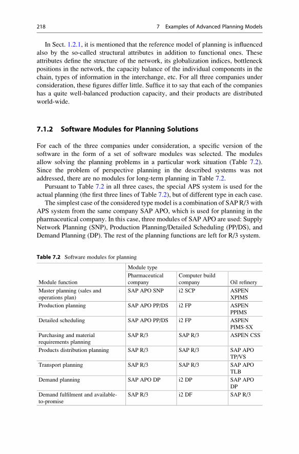
In Sect. 1.2.1, it is mentioned that the reference model of planning is influenced
also by the so-called structural attributes in addition to functional ones. These
attributes define the structure of the network, its globalization indices, bottleneck
positions in the network, the capacity balance of the individual components in the
chain, types of information in the interchange, etc. For all three companies under
consideration, these figures differ little. Suffice it to say that each of the companies
has a quite well-balanced production capacity, and their products are distributed
world-wide.
7.1.2 Software Modules for Planning Solutions
For each of the three companies under consideration, a specific version of the
software in the form of a set of software modules was selected. The modules
allow solving the planning problems in a particular work situation (Table 7.2).
Since the problem of perspective planning in the described systems was not
addressed, there are no modules for long-term planning in Table 7.2.
Pursuant to Table 7.2 in all three cases, the special APS system is used for the
actual planning (the first three lines of Table 7.2), but of different type in each case.
The simplest case of the considered type model is a combination of SAP R/3 with
APS system from the same company SAP APO, which is used for planning in the
pharmaceutical company. In this case, three modules of SAP APO are used: Supply
Network Planning (SNP), Production Planning/Detailed Scheduling (PP/DS), and
Demand Planning (DP). The rest of the planning functions are left for R/3 system.
Table 7.2 Software modules for planning
Module function
Module type
Pharmaceutical
company
Computer build
company Oil refinery
Master planning (sales and
operations plan)
SAP APO SNP i2 SCP ASPEN
XPIMS
Production planning SAP APO PP/DS i2 FP ASPEN
PPIMS
Detailed scheduling SAP APO PP/DS i2 FP ASPEN
PIMS-SX
Purchasing and material
requirements planning
SAP R/3 SAP R/3 ASPEN CSS
Products distribution planning SAP R/3 SAP R/3 SAP APO
TP/VS
Transport planning SAP R/3 SAP R/3 SAP APO
TLB
Demand planning SAP APO DP i2 DP SAP APO
DP
Demand fulfilment and available-
to-promise
SAP R/3 i2 DF SAP R/3
218 7 Examples of Advanced Planning Models
A slightly more complicated version is used at the computer build company. Here
the functions of production and demand planning are performed by the following
modules: Supply Chain Planner (SCP), Factory Planner (FP), and Demand Planning
(DP). In addition, the APS system type i2 Technologies is assigned with the function
of Demand Fulfilment (DF).
Application of i2 Technologies system is associated here with a very large scope
of production planning and the need for frequent changes in planning. Indeed, due
to the considerable amount of incoming components and their rapid obsolescence,
the need to take into account the needs of different customers, it requires high-speed
operation of the planning system, which is provided by i2 Technologies system due
to so-called special fast platform (i2 Agile Business Process Platform) provided.
The most complex system is used in the example of planning for the oil refinery.
In this case, for the purpose of production planning PIMS (Process Industry
Modelling System) software from ASPEN is used. It is designed specially for the
oil industry. This software allows optimizing the raw materials and semi-finished
products cleaning and blending processes, maintaining their balance and optimizing
costs. The optimization is carried out in the framework of both linear and non-linear
programming with powerful computing programs ILOG CPLEX from IBM and
XPRESS from Dash Optimization.
For periodic planning (scheduling), PPIMS-SX version of PIMS software is
used. It allows for scheduled payments with the horizon of 36 weeks. XPIMS
product is an add-on of PIMS, providing planning optimization of joint operation
of several enterprises that are located geographically in different places. CSS
(Crude Scheduling System) module based on PIMS module is used for crude oil
procurement planning.
In this example, for the distribution and transportation planning, as well as
demand planning SAP APO modules are used, despite the fact that the relevant
modules are also available in dedicated system ASPEN. Perhaps, this is due to the
history of the information system implementation at the enterprise. The role of SAP
R/3 system in the planning is reduced to the demand (order) fulfilment in this case.
7.1.3 Planning Modules Interaction
Each cycle of planning in any of the above variant of planning starts with demand
planning. The activity on the market of each company in this example has its
own peculiarities. In particular, the pharmaceutical company operates mainly by
contracts with a lead-time horizon of 9–12 weeks in average. The level of demand
for oil refinery products and supplies of crude oil for it are determined monthly
within some possible limits. In addition, the price limits for raw materials and
finished products are forecasted. The demand at the computer build company is
distinguished by rapid changes resulting in market analysis to be carried out either
weekly or even twice a week.
Based on the forecasts made for sales, the so-called master planning is performed,
which is actually the development of sales and operations plan. This plan is the basis
7.1 Joint Operation Model of APS System and ERP System from SAP R/3 219
for all further planning process and for the enterprises of different industries, the
sales plan horizon differs significantly. For example, at the computer build company,
themaster planning is performed everyweekwith the planning horizon equalling the
longest expected delivery time for components. At the oil refinery, the sales plan can
be developed simultaneously for different horizons, 3–36 months. In this case, the
basic long-term plan is adjusted periodically by drawing up short-term plans. The
pharmaceutical company draws up sales plans with the 24-months horizon. This
company extensively uses vendor managed inventory (VMI), which allows fulfilling
almost all their possible demand.
Based on the sales plan, optimal (including price, speed of delivery, reliability of
supply, etc.) plans for raw material orders are developed. For example, the com-
puter build company makes or corrects this plan every business day and the set of
ordered parts and materials meet the demand rather strictly.
The pharmaceutical company has the ability to obtain raw materials from a
number of suppliers in different countries. This allows optimizing the cost of raw
materials taking into account the peculiarities of the tax legislation of these
countries. In addition, it is possible to vary the supply of raw material kinds and
consequently to achieve contractual product composition by adjusting production
processes.
A similar situation occurs with crude oil supplies. Furthermore, in this case the
choice of oil grade, the possibility of its transportation within the ordering period
and the cost of such transportation is of great importance. The possible differences
in finished product costs in different geographical markets, etc., must also be borne
in mind. The fundamental specificity of operation with oil led to the necessity to
develop the above-mentioned software CSS, which takes into account most of the
factors that affect the optimal planning of crude oil procurement.
Production planning is based on the control-aggregated volumes of sales plan.
First of all, the planning requires specifying of sales plan indicators for specific
types of products, and secondly, availability of complete data on products and
related processes. These data are transmitted from SAP R/3 system to production
planning modules in the form of so-called Production Process Model (PPM) (see
Sect. 5.1.1).
For the pharmaceutical company, thismodel is amaster recipe of the corresponding
version and the composition of manufactured products. Since the process does
not change during computer building, the production process model is simplified
here and contains only the configuration of a product of each standard size. In oil
processing, on the contrary, the composition of manufactured products varies little,
but for each kind of raw material the relevant parameters are set in the production
process model.
At the stage of finished products dispatch to consumers, optimization issues
do usually not arise. Therefore, both the pharmaceutical company and the computer
company use mainly the modules of basic ERP system R/3 for this purpose.
However, for the oil refinery the optimization issues of dispatch are as important
as of obtaining raw materials. Well-formed lots according to their destination can
significantly reduce the cost of delivery. From Table 7.2 we see that for this purpose
220 7 Examples of Advanced Planning Models
the optimal planning modules of SAP APO system are used, which are well
coordinated with the basic R/3 system. In any case, the paperwork for dispatch is
done by means of the ERP system.
7.2 Reference Model of Production Planning for InstrumentEngineering Plant
This section describes the planning model developed in 2008–2010 by Moscow
company Infosoft with the author’s participation.
7.2.1 Initial Planning Status Analysis
The sequence of the reference model development primarily corresponded to the
methodology outlined above in Sect. 1.2.2. According to this methodology, first the
current state of the planning system (state AS-IS) was studied and the tool (BPwin
system) was selected to develop the model. With the help of this tool a number
of documents describing the information flows and decision flows in production
planning were developed.
It was found that in the planning of core production, for most of the products
(Production No. 1) the assembly-to-order planning method is used. Simultaneously,
some products (Production No. 2) are produced as part of manufacturing strategy
“make-to-stock”. All kinds of products are made in the framework of push-type
production. Production of the core products is characterized by high instability,
where the flow of changes in design and technological documentation, made by the
change notices (Sect. 5.1.1), amounts up to several tens per week.
Within the planning system, three production plans are developed: sales and
operation plan, master plan and production schedules. The purpose of the first of
them is to define the annual production volumes with an outlook for 1–2 years, as
well as verification of capacity utilization for a long period broken down by months.
The master plan is generated annually on monthly basis according to the output
plan. In this case, from the output plan the orders, which to be fulfilled in the
planning year, and the orders, which to be launched in the planning year, are
selected. The due dates of works in the master plan are calculated from the date
of output in the sales and operation plan back in time to the determination of launch
dates.
Based on the master plan, the production site schedules are made with break-
down by day. The schedules are prepared from the launch date forward in time.
Under this model, similarly with Table 7.1, a table of functional attributes
(Table 7.3) was made. Due to the fact that at the same enterprise there are actually
two different types of production for the products for different applications with
different scales and production strategies, the attributes are described individually
for each of these productions.
7.2 Reference Model of Production Planning for Instrument Engineering Plant 221

Let us compare the values of functional attributes for two existing production
sites of this enterprise, as well as the values of these attributes with the similar
attributes of the previous example in Sect. 7.1.1. Obviously, for both productions
and especially for production No. 2 in Table 7.3, the closest example is the
computer build company in Table 7.1. The values of the attributes of the materials
used and the product life cycle performance are practically the same.
Production No. 2 is a set of cell manufacturing sites (type 4 in Sect. 1.2.1),
similar to sub-assemblies at the computer build company. At the same time in
production No. 1, the cell manufacturing is used only at the assembly stages and the
parts machining is performed by multipurpose machines at the production sites of
specific jobs.
In general, production No. 2 differs from the computer build company of the
previous example only by much smaller production scale, which, however, is still
serial. Production No. 1 distinguishes itself from production No. 2 not only by
small-serial but also by high instability (attribute 7) caused by various factors and
principally by frequent changes in documentation.
When making the description of AS-IS state, as recommended by methodology
for a reference model (Sect. 1.2.2), the nature of information flow at the enterprise
was studied, in particular its aspects such as the list of main inputs of a business
Table 7.3 Functional attributes of the production sites of the instrument engineering plant
Attribute type
Attribute value
Production
No. 1 (assembly-to-order)
Production
No. 2 (make-to-stock)
1. Nomenclature of incoming materials
and raw materials
Large (over 1000) Small (less than 100)
2. Duration and reliability of delivery Long, low reliability Long, reliable
3. Shelf life of materials and
components
Short Long
4. Type of production Multipurpose and cell
manufacturing
Cell manufacturing
5. Size of lot Variable Fixed
6. Production bottle-neck Known Non
7. Documentation stability Instable Stable
8. Number of processing stages 7–10 2–3
9. Frequency of dispatch By orders By orders
10. Sales calculation By orders By forecast
11. Seasonal demand fluctuations Non By quarters
12. Duration of stable output Several years Several years
13. Number of standard modifications Several Many
14. Availability of custom special
properties
Yes No
15. Material flow Processing and assembly Processing and
assembly
222 7 Examples of Advanced Planning Models
process, transformation of information in business process, etc. It was found that the
enterprise applied the ERP system of its own design, which provided logging of
design documentation, accounting and data storage of material procurement, sales,
accounts and finance departments. Archiving of orders in the system was reduced
mainly to their registration.
The input information for scheduling, besides orders, is also the so-called card
file that contains a list of products manufactured in the shop for current “active”
version. Recall (Sect. 5.1.1) that active current version is the design documentation
with regard to the change notices in effect at that moment. The card file also
indicates the availability of products manufactured by various versions. The card
file is corrected based on the design and technological change notices, and the
results are used in performance of operations.
In accordance with the developed planning schedules and processes for each
manufactured item of the plan, the route sheets are generated that accompany the
products at all stages of production from the receipt of materials or workpieces until
submitting to the quality control department. After delivery of good products the
relevant checkoffs are made in the schedules, and in case of defective products the
defect certificate is drawn specifying the reasons therefore. Good products are
delivered to the warehouse and transferred against an invoice. The situation in the
shop is regularly monitored and regulated by the planning and operating bureau
(POB).
Analysis of the AS-IS state revealed a number of drawbacks in business process
of production planning. First of all, the existence of a significant number of
scattered throughout the enterprise, unrelated and poorly controlled orders leads
to data uncertainty about the real state of production. In the master plan based on the
annual output plan the job tasks for the shops have too aggregative nature, which
causes their failure to be completed in time through many items. The production
scheduling directly by the shops foremen is often subjective and does not contribute
to high performance.
7.2.2 Decision Support Database
The results of the AS-IS state analysis within the reference model led to develop-
ment of a number of suggestions and documents describing the planning business
process for the TO-BE state. For the purpose of order management it was suggested
to create a special planning authority allowing concentration of all the external
and internal orders and ensure their registration and recording of actual fulfilment.
It was suggested to establish plan types that are standard for ERP systems—
long-term plan (sales and operations), master plan, material requirement plan and
operational plan.
When developing the planning model for the TO-BE state both the enterprise’s
wishes and the basic principles of advanced planningwere taken into account, namely
(Sect. 1.4): use of flexible horizon, compulsory analysis of available information
in order to support and optimize the decisions made, as well as consideration of
7.2 Reference Model of Production Planning for Instrument Engineering Plant 223
various constraints, especially in equipment capacities, directly in the planning
process.
In particular, it was proposed to make the master plan not once a year but review
it regularly with some interval (a month) and corresponding shift in phase of
accomplishment. In preparation of the material requirement plan it was suggested
to consider the requirements of MRP as well as the intensity of the order in
accordance with the definition of intensity in Sect. 2.4.1 in sequence of individual
order fulfilment. Further, simultaneously the utilization ratio of individual, the
most loaded work centers were tested according to the procedure described in
Mauergauz (2007).
For planning with regard to its optimization elements, it was decided to use the
opportunity to create a decision-support database (Sect. 5.1.4) directly within one
active ERP system at the enterprise. This organization of the information system
allowed not developing a special APS system but simply extending the functional-
ity of the existing system.
A decision-support database is, as described above in Sect. 5.1.4, analytical basis
of any information system. This basis, as has been said, can be arranged separately
from the main transactional database and can be combined or even aligned with the
latter. In this example, the database of the analysis system is designed as a special
set of tables under the control of the same DBMS, which controls the main
transactional database. Figure 7.2 shows the databases tables for decision-making
in planning and their interaction pattern.
The central table of the database is table “Orders”, the records of which can be of
two types—agreements and production kits. In the first case, the orders are fulfilled
for specific external consumers, in the second case the production kits are ordered
for “make-to-stock” production and the subsequent sale. Each order can have a
number of items, i.e. lines that contain information about a product, its quantity,
composition, cost and so on, reflected in table “Order composition”. The sequence
of supplies for each order item is specified in table “Delivery schedule”.
The individual configuration (composition) for each order item is selected or
created from a set of options recorded in table “Order configuration”. The objects of
this configuration are the parts and assembly units (PAU), which may be included
into other assembly units by different ways.
Each PAU object has its own design and technological history. Table “History of
PAU” contains a list of various versions of design, and table “History of SPR”
contains a list of versions of the summary process routes for each PAU object.
Source documents (drawings, processes, change notices, etc.) related to each of the
versions contained in the main (transactional) database are not shown here.
A set of PAU objects and codes of their current (active) versions for each
configuration of the order is placed in a separate Production Process Model
(PPM) as described above in Sect. 5.1.1. Each line of the delivery schedule has
its own PPM.
After preparing the PPM and delivery schedules, it is possible to make planning
decisions that are executed in the form of master plan. In this plan, each type of
product (PAU code) corresponds to a certain number of planned items, each of
224 7 Examples of Advanced Planning Models
which is designed to fulfil the orders according to the delivery schedule. The
information about the PPM, due date and number of products received from the
delivery schedule during development of the schedule is referenced and can be
updated. During implementing the schedule the status of a scheduled item may vary
depending on the production situation.
Agreement (for ordering agreement)Order codeDate of agreementOrder type (agreement or set)
Status (approved, signed off etc.)
Orders
Order configuration codeOrder codeOrder item codeTotal quantityStatus (approved, from stock etc.)
Order composition
Order item codeDue datePPM codeQuantityPPM type (complete, non-
complete, maintenance etc.)
Delivery schedule
PAU codeVersion date
Record No
PAU codeVersion date
Record No.
History of PAU
PAU codePlan item codeOrder codeOrder item codeDue datePPM codeQuantityStatus (approved, signed off, from stock etc.)
Master plan
PAU code (where included)PAU code (what)Quantity Measuring unitOrder configuration code
Order configuration
Output lot numberPlan item codeRelease lot number
Number interval of production kits
Output lot
Release lot numberTotal quantityRelease date
Release lot
History of SPR
PAU history codeSPR history codePAU codePPM code
Production Process
Model (PPM)
Fig. 7.2 Tables of the database for planning decision-making
7.2 Reference Model of Production Planning for Instrument Engineering Plant 225
Several planning items usually with the same date of fulfilment are grouped into
an output lot. In table “Output lot” each plan item is assigned with number interval
of PAU sets, which then allows tracing the life cycle of each instance of the product.
The release of a new lot of finished product into production often makes sense to
be carried out simultaneously for several output lots. This allows you to increase the
size of production lots for many types of PAU, which are common components of
different orders for finished products, including the processed ones according to
different PPM. Therefore, in this example, special table “Release lot” is provided.
This approach in planning database organization is described in more detail in
Mauergauz (2007).
7.3 Mathematical Model in Chemical Industry
The described model was proposed in the article of Kondili et al. (1993) and until
present has been the focus of attention of many studies by various authors, for
example Ierapetritou and Floudas (1998) and others.
7.3.1 Analytical Structure of Model
Let us consider the structure of production shown in Fig. 7.3 representing the
simplest variant of chemical production. According to the classification in Sect.
1.3.1, this structure is type 3c—repetitive serial production line that produces core
products and by-products. In this model, there is a special piece of equipment for
each manufacturing operation, and upon completion of an operation the product is
discharged into an appropriate buffer tank. For different orders the line can be set up
and manufacture products with different properties.
In accordance with the above terminology we will call each necessary process
operation as a job or task with number i, and each process installation—a machine
or unit with number j. In the example in Fig. 7.3, each unit is designed to perform
only one type of tasks. During the manufacturing process the raw material fed to the
line input is first converted into semi-product with various degree of finishing and
then into the core or by-products. To perform each operation, a machine is loaded
with some quantity of raw material or semi-products, and after the operation the
obtained product lot is discharged into the relevant tank. We further assume that the
Core products
Raw material 2 By-products
OrdersMixer Reactor Rectifier
Raw material 1
Buffer 1 Buffer 2
1 2
Fig. 7.3 The simplest structure of chemical production
226 7 Examples of Advanced Planning Models

initial raw materials, semi-finished products, stored in buffer tanks, as well as
finished products represent a state of the processed product.
In the paper of Kondili et al. (1993), it was suggested to name the structure like
shown in Fig. 7.3 the production state-task network (STN). Using the diagram of
this structure it is not necessary to specify particular manufacturing equipment
directly but just to enumerate all the states of the products undergoing the
processing, as well as the jobs for transferring these products from the current
state to the subsequent one. Figure 7.4 shows an example of an analytical structure
of this type of model (Ierapetritou and Floudas 1998).
As can be seen from Fig. 7.4, in the result of manufacture two finished products
should be received of three types of raw materials, and product 2 is a core product
(received at the end of the manufacturing process), and product 1 is a by-product.
For manufacturing operations, which involve several types of raw materials or
semi-finished products, Fig. 7.4 shows the data on their percentage in an operation.
After operation “reaction 2” some part of the resulting product is transferred
for further processing and some part is the product ready for immediate sale.
The wastes resulting from the separation are included in the reprocessing during
“reaction 3”.
The main difference of the diagram in Fig. 7.4 from the previous diagram in
Fig. 7.3 is that in the first one the number of processing units (machines) is not
necessarily equal to the number of process operations, but may be not only greater
than the number of operations but less than this number. It is obvious that if the
number of machines for a particular operation is greater than one, it does not change
the type of production 3b of the entire repetitive serial production line.
If the total number of machines of the production line is less than the number of
operations, this means that one or more machines must provide performance of
different production operations, i.e. according to the terminology introduced above,
perform multiple tasks. In this example, each of three reactions in Fig. 7.4 can be
performed on any of the two available reactor-machines, while for heating and
80%
20%50%
50%
Semi-productAB
10%
90%
60%
Raw B
Semi-product BC
60%Heated raw A
Raw AHeating Reaction 2
40%
Reaction 1
Raw C
Finished
product 1
40%
Reaction 3
Crude product
E
Separation
Finished
product 2
1
2
3
4
Fig. 7.4 Analytical structure of STN-model [based on Ierapetritou and Floudas (1998)]
7.3 Mathematical Model in Chemical Industry 227
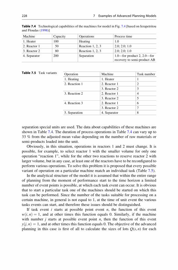
separation special units are used. The data about capabilities of these machines are
shown in Table 7.4. The duration of process operations in Table 7.4 can vary up to
33 % from the adjusted mean value depending on the number of raw materials or
semi-products loaded into the unit.
Obviously, in this situation, operations in reactors 1 and 2 must change. It is
possible, for example, to select reactor 1 with the smaller volume for only one
operation “reaction 1”, while for the other two reactions to reserve reactor 2 with
larger volume, but in any case, at least one of the reactors have to be reconfigured to
perform various operations. To solve this problem it is proposed that every possible
variant of operation on a particular machine match an individual task (Table 7.5).
In the analytical structure of the model it is assumed that within the entire range
of planning from the moment of performance start to the time horizon a limited
number of event points is possible, at which each task event can occur. It is obvious
that to start a particular task one of the machines should be started on which this
task can be performed. Since the number of the tasks suitable for processing on a
certain machine, in general is not equal to 1, at the time of unit event the various
tasks events can start, and therefore these issues should be distinguished.
If task event i starts at possible point event n, the function of this event
w i; nð Þ ¼ 1, and at other times this function equals 0. Similarly, if the machine
with number j starts at possible event point n, then the function of this event
y j; nð Þ ¼ 1, and at other times this function equals 0. The objective of the advanced
planning in this case is first of all to calculate the sizes of lots Q(s, n) for each
Table 7.4 Technological capabilities of the machines for model in Fig. 7.4 [based on Ierapetritou
and Floudas (1998)]
Machine Capacity Operations Process time
1. Heater 100 Heating 1.0
2. Reactor 1 50 Reaction 1, 2, 3 2.0; 2.0; 1.0
3. Reactor 2 80 Reaction 1, 2, 3 2.0; 2.0; 1.0
4. Separator 200 Separation 1.0—for product 2, 2.0—for
recovery to semi-product AB
Table 7.5 Task variants Operation Machine Task number
1. Heating 1. Heater 1
2. Reaction 1 2. Reactor 1 2
3. Reactor 2 3
3. Reaction 2 2. Reactor 1 4
3. Reactor 2 5
4. Reaction 3 2. Reactor 1 6
3. Reactor 2 7
5. Separation 4. Separator 8
228 7 Examples of Advanced Planning Models
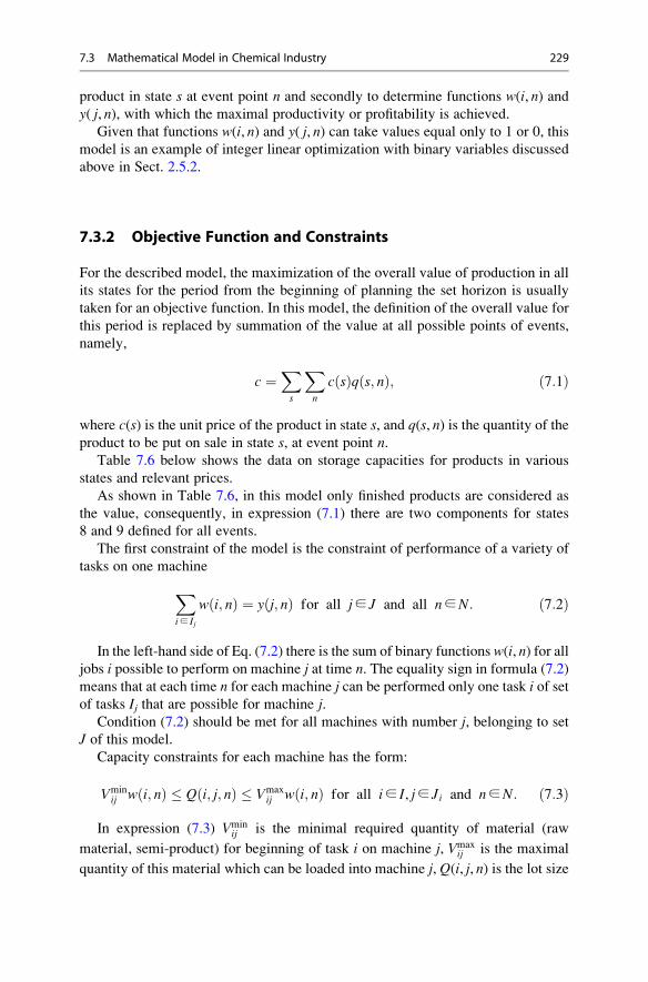
product in state s at event point n and secondly to determine functions w(i, n) andy( j, n), with which the maximal productivity or profitability is achieved.
Given that functions w(i, n) and y( j, n) can take values equal only to 1 or 0, this
model is an example of integer linear optimization with binary variables discussed
above in Sect. 2.5.2.
7.3.2 Objective Function and Constraints
For the described model, the maximization of the overall value of production in all
its states for the period from the beginning of planning the set horizon is usually
taken for an objective function. In this model, the definition of the overall value for
this period is replaced by summation of the value at all possible points of events,
namely,
c ¼Xs
Xn
c sð Þq s; nð Þ; ð7:1Þ
where c(s) is the unit price of the product in state s, and q(s, n) is the quantity of theproduct to be put on sale in state s, at event point n.
Table 7.6 below shows the data on storage capacities for products in various
states and relevant prices.
As shown in Table 7.6, in this model only finished products are considered as
the value, consequently, in expression (7.1) there are two components for states
8 and 9 defined for all events.
The first constraint of the model is the constraint of performance of a variety of
tasks on one machineXi∈ Ij
w i; nð Þ ¼ y j; nð Þ for all j∈ J and all n∈N: ð7:2Þ
In the left-hand side of Eq. (7.2) there is the sum of binary functions w(i, n) for alljobs i possible to perform on machine j at time n. The equality sign in formula (7.2)
means that at each time n for each machine j can be performed only one task i of setof tasks Ij that are possible for machine j.
Condition (7.2) should be met for all machines with number j, belonging to set
J of this model.
Capacity constraints for each machine has the form:
Vminij w i; nð Þ � Q i; j; nð Þ � Vmax
ij w i; nð Þ for all i∈ I, j∈ Ji and n∈N: ð7:3Þ
In expression (7.3) Vminij is the minimal required quantity of material (raw
material, semi-product) for beginning of task i on machine j, Vmaxij is the maximal
quantity of this material which can be loaded into machine j, Q(i, j, n) is the lot size
7.3 Mathematical Model in Chemical Industry 229
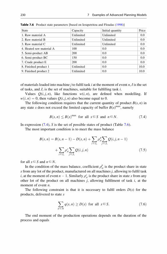
of materials loaded into machine j to fulfil task i at the moment of event n, I is the setof tasks, and Ji is the set of machines, suitable for fulfilling task i.
Values Q(i, j, n), like functions w(i, n), are defined when modelling. If
w i; nð Þ ¼ 0, then values Q(i, j, n) also become equal to 0.
The following condition requires that the current quantity of product B(s, n) inany state s does not exceed the limited capacity of buffer B(s)max, namely
B s; nð Þ � B sð Þmaxfor all s∈ S and n∈N: ð7:4Þ
In expression (7.4), S is the set of possible states of product (Table 7.6).
The most important condition is to meet the mass balance
B s; nð Þ ¼ B s, n� 1ð Þ � D s; nð Þ þXi∈ Is
ρpsi
Xj∈ Ji
Q i, j, n� 1ð Þ
þXi∈ Is
ρ csi
Xj∈ Ji
Q i; j; nð Þ ð7:5Þ
for all s∈ S and n∈N.In the condition of the mass balance, coefficient ρpsi is the product share in state
s from any lot of the product, manufactured on all machines j, allowing to fulfil taski, at the moment of event n� 1. Similarly ρcsi is the product share in state s from any
other lot of the product on all machines j, allowing fulfilment of task i, at themoment of event n.
The following constraint is that it is necessary to fulfil orders D(s) for the
products, delivered to state sXn∈N
q s; nð Þ � D sð Þ for all s∈ S: ð7:6Þ
The end moment of the production operations depends on the duration of the
process and equals
Table 7.6 Product state parameters [based on Ierapetritou and Floudas (1998)]
State Capacity Initial quantity Price
1. Raw material A Unlimited Unlimited 0.0
2. Raw material B Unlimited Unlimited 0.0
3. Raw material C Unlimited Unlimited 0.0
4. Heated raw material A 100 0.0 0.0
5. Semi-product AB 200 0.0 0.0
6. Semi-product BC 150 0.0 0.0
7. Crude product E 200 0.0 0.0
8. Finished product 1 Unlimited 0.0 10.0
9. Finished product 2 Unlimited 0.0 10.0
230 7 Examples of Advanced Planning Models
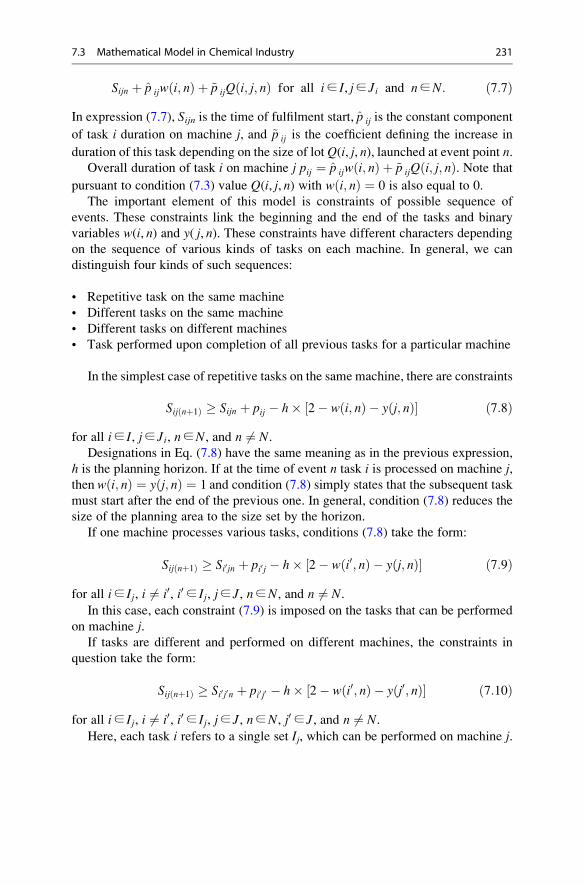
Sijn þ p ijw i; nð Þ þ ~p ijQ i; j; nð Þ for all i∈ I, j∈ Ji and n∈N: ð7:7Þ
In expression (7.7), Sijn is the time of fulfilment start, p ij is the constant component
of task i duration on machine j, and ~p ij is the coefficient defining the increase in
duration of this task depending on the size of lot Q(i, j, n), launched at event point n.Overall duration of task i on machine j pij ¼ p ijw i; nð Þ þ ~p ijQ i; j; nð Þ. Note that
pursuant to condition (7.3) value Q(i, j, n) with w i; nð Þ ¼ 0 is also equal to 0.
The important element of this model is constraints of possible sequence of
events. These constraints link the beginning and the end of the tasks and binary
variables w(i, n) and y( j, n). These constraints have different characters dependingon the sequence of various kinds of tasks on each machine. In general, we can
distinguish four kinds of such sequences:
• Repetitive task on the same machine
• Different tasks on the same machine
• Different tasks on different machines
• Task performed upon completion of all previous tasks for a particular machine
In the simplest case of repetitive tasks on the same machine, there are constraints
Sij nþ1ð Þ � Sijn þ pij � h� 2� w i; nð Þ � y j; nð Þ½ � ð7:8Þ
for all i∈ I, j∈ Ji, n∈N, and n 6¼ N.Designations in Eq. (7.8) have the same meaning as in the previous expression,
h is the planning horizon. If at the time of event n task i is processed on machine j,then w i; nð Þ ¼ y j; nð Þ ¼ 1 and condition (7.8) simply states that the subsequent task
must start after the end of the previous one. In general, condition (7.8) reduces the
size of the planning area to the size set by the horizon.
If one machine processes various tasks, conditions (7.8) take the form:
Sij nþ1ð Þ � Si0jn þ pi0j � h� 2� w i0; nð Þ � y j; nð Þ½ � ð7:9Þ
for all i∈ Ij, i 6¼ i0, i0 ∈ Ij, j∈ J, n∈N, and n 6¼ N.In this case, each constraint (7.9) is imposed on the tasks that can be performed
on machine j.If tasks are different and performed on different machines, the constraints in
question take the form:
Sij nþ1ð Þ � Si0j0n þ pi0j0 � h� 2� w i0; nð Þ � y j0; nð Þ½ � ð7:10Þ
for all i∈ Ij, i 6¼ i0, i0 ∈ Ij, j∈ J, n∈N, j0 ∈ J, and n 6¼ N.Here, each task i refers to a single set Ij, which can be performed on machine j.
7.3 Mathematical Model in Chemical Industry 231
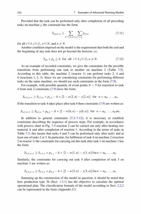
Provided that the task can be performed only after completion of all preceding
tasks on machine j, the constraint has the form
Sij nþ1ð Þ �X
n0 ∈N, n0�n
Xi0 ∈ Ij
pi0j0n0 ð7:11Þ
for all i∈ I, j∈ Ji, n∈N, and n 6¼ N.Another condition imposed on the model is the requirement that both the end and
the beginning of any task does not go beyond the horizon, i.e.
Sijn þ pij � h for all i∈ I, j∈ Ji, n 6¼ N: ð7:12Þ
As an example of recorded constraints, we give the constraints for the possible
transitions from performing one task to another on machine 2 (Table 7.5).
According to this table, the machine 2 (reactor 1) can perform tasks 2, 4 and
6 (reactions 1, 2, 3). Since we are considering constraints for performing different
tasks on the same machine, we should use such constraints in the form (7.9).
For example, with possible quantity of event points N ¼ 5 for transition to task
4 from task 2 constraints (7.9) have the form:
S4,2,nþ1 � S2,2,n þ p2,2 � h� 2� w 2; nð Þ � y 2; nð Þ½ � for n ¼ n0, . . . , n4:
If the transition to task 4 takes place after task 6 then constraints (7.9) are written as:
S4,2,nþ1 � S6,2,n þ p6,2 � h� 2� w 6; nð Þ � y 6; nð Þ½ � for n ¼ n0, . . . , n4 etc:
In addition to general constraints (7.2–7.12), it is necessary to establish
constraints describing the sequence of process steps. For example, in accordance
with process chart in Fig. 7.5 reaction 2 can be carried out only after heating raw
material A and after completion of reaction 1. According to the terms of tasks in
Table 7.5, this means that tasks 4 and 5 can be performed only after task1 and at
least one of tasks 2 or 3. In particular, for fulfilment of task 4 on machine 2 (reaction
2 in reactor 1) the constraints for carrying out this task after task 1 on machine 1 has
the form:
S4,2,nþ1 � S1,1,n þ p1,1 � h� 2� w 1; nð Þ � y 1; nð Þ½ � forn ¼ n0, . . . , n4:
Similarly, the constraints for carrying out task 4 after completion of task 3 on
machine 3 are written as:
S4,2,nþ1 � S3,3,n þ p3,3 � h� 2� w 3; nð Þ � y 3; nð Þ½ � forn ¼ n0, . . . , n4:
Summing up the construction of the model in question, it should be noted that
here production type 3b (Sect. 1.3.1) has the objective to calculate the optimal
operational plan. The classification formula of the model according to Sect. 2.2.2
can be represented in the form (Appendix C):
232 7 Examples of Advanced Planning Models
F��prec, batch, pi ∈ p
i: pi
h i��fmax: ð7:13Þ
In expression (7.13) according to the designations in Appendix C: F is the flow
shop, prec—presence of constraints on process operations sequence, batch—using
the manufacture lots for fulfilment of tasks, pi ∈ pi: pi
h imeans that duration pi of
each task i can be in the range from pito pi and fmax—maximization of the objective
function of value cost.
7.3.3 Some Results of Modelling
In modelling, as a starting parameter the number of possible event points N is set,
which may vary and lead to somewhat different results of optimization. In the paper
of Ierapetritou and Floudas (1998), the results for N ¼ 5 and N ¼ 6 are given,
the differences between them are small. The volume of computational work is
characterized by a number of independent variables of the problem and constraints.
In the described model, there are 260 continuous variables, 40 binary variables and
374 constraints inequalities.
The results of modelling in the form of Gantt diagram are shown in Fig. 7.5. In
this figure, the numbers of tasks and amount of product in the relevant state
produced on each of four machines are presented. The duration of horizon h is
accepted to be 8 h. As can be seen from Fig. 7.5, the optimal plan provides the start
of both reactors at the beginning of the shift to perform reaction 1 (tasks 2 and 3).
By the end of the processes in the reactors it is planned to heat raw material A in the
heater and then run the reactors for sequential performance of reaction 2 (tasks 4, 5)
and reaction 3 (tasks 6, 7). The resulting crude product E (state 7) is fed to the
separator for cleaning (task 8). The presence of buffer capacities for semi-product
BC (state 6) allows processing the semi-finished product in reaction of 2 (tasks 4, 5)
in two stages, as shown in Fig. 7.5.
5
0 1 2 3 4 5 6 7 8
Separator
Reactor 2
Reactor 1
Heater1 1
2
3
4 6
7
4
5
65 72 54 35
88
658
47 28
40 45 34 22
Fig. 7.5 Gantt diagram of subsequent task performance [based on Ierapetritou and Floudas
(1998)]
7.3 Mathematical Model in Chemical Industry 233
Obviously, the work plan for the subsequent shift should be different from the
plan in Fig. 7.5 because the initial amount of the product in various states will differ
from the values in Table 7.6, which were taken as 0. Generally speaking, the shift
task should be linked to a production task assigned for longer duration, for example,
with the master plan.
In the paper by Li and Ierapetritou (2009), the schedule model for the described
example expands considering its collaboration with the mathematical model of the
schedule, which is valid at least for a few shifts. In this case, the objective function
schedule optimization is different from the function of shift schedule.
It should be noted that most of the studies on production scheduling theory
published in recent years, in contrast to earlier studies, usually regard planning
as a process consisting of two steps. This is due to the understanding of the fact that
at different stages the planning criteria differ (Tables 2.5–2.7). In the article by
Li and Ierapetritou (2009) the objective function for the schedule is to minimize
the integrated storage cost, loss of profits due to the inability to fulfil orders and
immediate production costs. When preparing the shift task the cost of production is
actually minimized.
Unlike the conventional optimization of each stage in Li and Ierapetritou (2009)
attempts are made to harmonize the optimal calendar plan and all schedules for the
corresponding period by planning in several (30–40) iterations. The obtained results
show that the proposed model can provide a good match between the demand for
core product (finished product 2) and its production.
An interesting result of this study is determination of the relationship between
the volume of by-products (finished product 1) output and core product 2 output
(Fig. 7.6). From the chart in Fig. 7.6, it follows that at first with the increase in
production of product 1 the yield of core product 2 also increases. If the value of
product 1 volume is about 55 units, the yield of product 2 reaches the maximum and
then decreases gradually. When the volume of product 1 reaches 70 units the yield
of product 2 drops dramatically and if the volume of product 1 is equal to 87 units, it
tends to zero.
This type of chart is easily explained from the perspective of equipment utiliza-
tion. In the left part of the chart, the equipment is not fully loaded and its capacity is
sufficient for simultaneous output growth for both products. With the volume of
product 1 of 55 units, the load reaches the possible maximum, and further growth
of this product is only possible by reducing the output of product 2. If the volume of
product 1 tends to 87 units, all production capacity is entirely used only for this
product and the further increase is impossible.
7.4 Rapid Supply Chain Reference Model in Clothing Industry
The study by Macedo (2000) considers a model of the supply chain, in which
requirements of “make-to-order” production are combined with the need of urgent
changes in production. This supply chain is called Fast Innovation Reinforcement
234 7 Examples of Advanced Planning Models
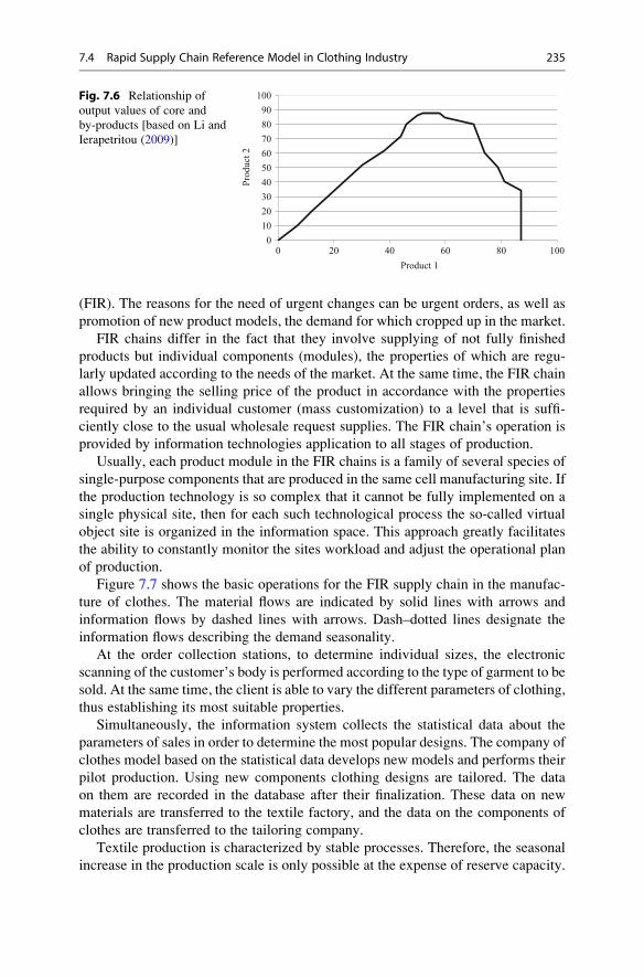
(FIR). The reasons for the need of urgent changes can be urgent orders, as well as
promotion of new product models, the demand for which cropped up in the market.
FIR chains differ in the fact that they involve supplying of not fully finished
products but individual components (modules), the properties of which are regu-
larly updated according to the needs of the market. At the same time, the FIR chain
allows bringing the selling price of the product in accordance with the properties
required by an individual customer (mass customization) to a level that is suffi-
ciently close to the usual wholesale request supplies. The FIR chain’s operation is
provided by information technologies application to all stages of production.
Usually, each product module in the FIR chains is a family of several species of
single-purpose components that are produced in the same cell manufacturing site. If
the production technology is so complex that it cannot be fully implemented on a
single physical site, then for each such technological process the so-called virtual
object site is organized in the information space. This approach greatly facilitates
the ability to constantly monitor the sites workload and adjust the operational plan
of production.
Figure 7.7 shows the basic operations for the FIR supply chain in the manufac-
ture of clothes. The material flows are indicated by solid lines with arrows and
information flows by dashed lines with arrows. Dash–dotted lines designate the
information flows describing the demand seasonality.
At the order collection stations, to determine individual sizes, the electronic
scanning of the customer’s body is performed according to the type of garment to be
sold. At the same time, the client is able to vary the different parameters of clothing,
thus establishing its most suitable properties.
Simultaneously, the information system collects the statistical data about the
parameters of sales in order to determine the most popular designs. The company of
clothes model based on the statistical data develops new models and performs their
pilot production. Using new components clothing designs are tailored. The data
on them are recorded in the database after their finalization. These data on new
materials are transferred to the textile factory, and the data on the components of
clothes are transferred to the tailoring company.
Textile production is characterized by stable processes. Therefore, the seasonal
increase in the production scale is only possible at the expense of reserve capacity.
0
10
20
30
40
50
60
70
80
90
100
0 20 40 60 80 100P
roduct
2
Product 1
Fig. 7.6 Relationship of
output values of core and
by-products [based on Li and
Ierapetritou (2009)]
7.4 Rapid Supply Chain Reference Model in Clothing Industry 235
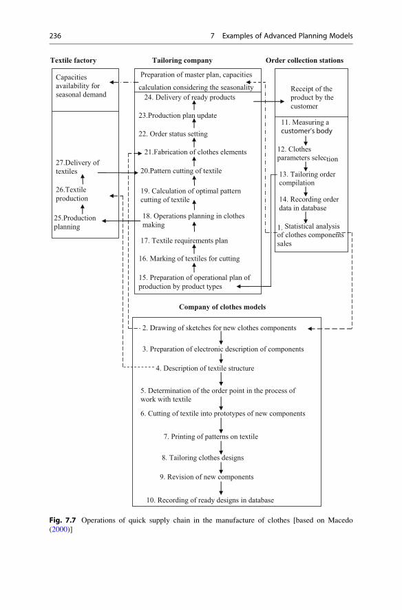
Preparation of master plan, capacities
calculation considering the seasonality
24. Delivery of ready products
23.Production plan update
21.Fabrication of clothes elements
20.Pattern cutting of textile
19. Calculation of optimal pattern
cutting of textile
22. Order status setting
18. Operations planning in clothes
making
17. Textile requirements plan
16. Marking of textiles for cutting
15. Preparation of operational plan of
production by product types
Receipt of the product by the
customer
11. Measuring a customer’s body
12. Clothes parameters selection
13. Tailoring order compilation
1. Statistical analysis of clothes components
sales
2. Drawing of sketches for new clothes components
14. Recording order
data in database
3. Preparation of electronic description of components
4. Description of textile structure
5. Determination of the order point in the process of work with textile
6. Cutting of textile into prototypes of new components
7. Printing of patterns on textile
8. Tailoring clothes designs
9. Revision of new components
10. Recording of ready designs in database
Capacities availability for seasonal demand
Tailoring companyTextile factory Order collection stations
Company of clothes models
27.Delivery of textiles
26.Textile
production
25.Production
planning
Fig. 7.7 Operations of quick supply chain in the manufacture of clothes [based on Macedo
(2000)]
236 7 Examples of Advanced Planning Models

Increased volume of tailoring can be possible in various ways including increasing
the number of personnel, their workload, etc.
The main difference and at the same time advantage of the described reference
model is that for the majority of its operations informational support is provided
in the form of special computer systems. Systems Lectra and Lawson Fashion
are mainly used for this purpose. The first one provides designing of clothes,
measurement of customer’s sizes and refinement of the designed by customer’s
requirements, as well as the optimal making-up and cutting of fabrics. The second
one is used for scheduling and managing the production of clothing on the shop
level. Both of these systems also provide data transfer between companies via
Internet.
Logistics methods of the quick supply chains are very popular now and being
intensively developed. A number of studies of this kind were published in the book
by Kestner et al. (2008).
7.5 Schedule Model for a Machine Shop
One of the most important and frequently discussed problems of planning is the
problem of optimal scheduling for the job shop (type 5a in Sect. 1.3.1). As a rule,
this category includes machine shops of machine-building plants, furniture
factories and other enterprises producing serial and small-serial complex products.
To manufacture parts of such products, it is often necessary to have the process
consisting of a number of successive machining operations, and the order of these
operations is arbitrary. The sequence of operation of this production is convenient
to display in the form of so-called mixed graph (Fig. 7.8).
The circles in Fig. 7.8 denote the operations performed on workpiece i onmachine j. For the convenience of graph construction the fictive general starting
point of schedule S and finishing point E are introduced. The processing time of
each operation are indicated as pij. The solid lines with arrows indicate the move-
ment of the lot of parts from one machine to another according to the procedure
specified by the process.
The dashed lines with arrows designate the possible procedure of processing
different lots of parts on a certain machine. For example, since each of three kinds
p 14p 24
0
0
0
p 24
p 14
p36p 35
p 25
p 23
p 31
p 21
p11
S 2,3
1,4
2,4 2,5
3,5 3,6
E2,1
1,1
3,1
Fig. 7.8 Oriented mixed graph of job shop production
7.5 Schedule Model for a Machine Shop 237
of parts requires processing on machine 1, then six variants of sequences of three
kinds of machining on this machine are possible:{1, 2, 3}, {1, 3, 2}, {2, 1, 3},
{2, 3, 1}, {3, 1, 2} and {3, 2, 1}. It is easy to see that each of these variants is shown
in Fig. 7.8 in the form of sequence of two dashed arrows. Each of these arrows
corresponds to the processing duration, such as shown for arrows relating to
machine 4.
The problem of the optimal scheduling, in terms of getting the best option of
mixed graph 7.8, is to make optimal choice of dashed arrows describing the
sequence of operations on each machine. Practically, this means that of all the
possible permutations of this sequence only one should be selected, which ensures
the best value of an objective function. Obviously, the choice of the optimal
sequence obtained this way depends primarily on the type of the objective function.
7.5.1 Schedule Model with Specified Processing Stages
In the model (Prilutsky and Vlasov 2007) it is assumed that at the beginning of the
planning period we know the list of orders subject to processing. Each order is a set
of interdependent jobs that are performed on the machines. Equipment units are
arranged in groups of interchangeable machines, which fulfil various stages of
processing, herewith the machines in the group can have different performance.
In general, to perform each job i, it should be processed sequentially on the
machines of each stage l, and for each job order the procedure of passing through
the stages may differ.
The latter means that each job i should match the collection (vector)
~ri ¼ r i1, ri2, . . . r
ik
� for r il ∈K; l ¼ 1, 2, . . . ki; i∈ I: ð7:14Þ
In Eq. (7.14) ril is the stage number, where the l-th operation of job i shall beperformed, K is a set of stages (equipment groups), and ki is the quantity of
operations for job i. For example, if there are four groups of equipment—(1) turning,
(2) drilling, (3) milling, and (4) grinding, and the process for part 1 provides
for sequential operations of milling, drilling, turning, and grinding then vector
~r1 ¼ 3; 2; 1; 4ð Þ. It is assumed that at the next stage the job can be performed on
any machine of this stage.
It is necessary to schedule the jobs performance on the machines, for which the
aggregate cost is minimal. This schedule is represented by a set of values Sijl of startmoments of operation l of job i on machine j. The time period, during which such
operation is performed, is determined by binary function value yijl. If the operationis performed, then yijl ¼ 1, if not— yijl ¼ 0. The sequence of the entire set of
operations is determined during scheduling and described by a set of serial numbers
zijl. The quantity of these numbers is equal to the total amount of all transactions for
all jobs.
238 7 Examples of Advanced Planning Models
7.5.2 Optimality Criteria and Constraints
In the paper by Prilutsky and Vlasov (2007), the schedule quality assessment is
determined by three main components: the cost of jobs on the machines, the cost of
setup, and penalties imposed on the system for violation of specified due dates. The
cost of all operations on the machines:
Xj∈ J
Xkil¼1
cpijlpijlyijl; ð7:15Þ
where cpijl is the cost of manufacture time unit for an operation on particular
equipment and pijl is the operation duration.
Similarly, the costs for setup excluding the dependence of setup duration on its
sequence
Xj∈ J
Xkil¼1
csijlsijlyijl; ð7:16Þ
where csijl is the cost of setup time unit for an operation on particular equipment and
sijl is the setup duration.
In this paper, it is assumed that non-observance of timely (directive given)
performance of each job leads to penalties, which for various jobs may depend on
the delay to various extents, that is, for each job they have the form:
gimax 0, Sijk þ pijk � di�
; ð7:17Þ
where gi is the penalty amount per 1 day of tardiness of job i, Sijk is the start moment
(date) of the last (k-th) operation performed on machine j for job i, pijk is the
duration of this operation in days, and di is the due date of job i.The first of the constraints of the described model is that each operation of any
job must be performed on a certain machine, that isXj∈ J
yijl ¼ 1 for all l ¼ 1, 2, . . . ki; i∈ I: ð7:18Þ
Besides, any operation of job i can be started only after completion of all
operations that precede it according to the process:
Sijl � Sij l�1ð Þ þ pij l�1ð Þ for all l ¼ 1, 2, . . . ki; i∈ I, j∈ J: ð7:19Þ
Similarly, any new operation l of job i on machine j can be started only after
completion of operation l’ of previous job i’ on this machine, and after the
corresponding setup, i.e.
7.5 Schedule Model for a Machine Shop 239
Sijl � Si0jl0 þ pi0jl0 þ sijl for all l
¼ 1, 2, . . . ki; l0 ∈ 1, 2 . . . ki0 ; i∈ I, i0 ∈ I, j∈ J: ð7:20ÞBy analysing the schedules quality criteria (7.15) and (7.16), we see that both of
these values are cost input. In this case, their aggregate value describes the criterion
of direct costs K1 (Table 2.3). At the same time, indicator (7.17) characterizes the
delay of job performance and meets criterion C1 in Table 2.2.
The simultaneous use of two such criteria to assess the quality of the schedule
makes it necessary to solve a multi-objective problem. Considering the formulation
of this problem in terms of usefulness (Sect. 4.1.3), we see that it corresponds to the
points of small-serial or serial production on the curve of the UV-diagram for
operational plans, for which it was just recommended to use multi-criteria approach
in Sect. 4.1.3.
Let us draw up a classification model according to Sect. 2.2.2, the same way as it
was done in Sect. 7.3.2:
J��prec, di��Fl c; Tð Þ: ð7:21Þ
In expression (7.21) according to the designations in Appendix C: J is the job shop
designation, prec is the presence of constraints for process sequence of operations,di is the directly set due date for jobs performance, and Fl(c, T) is the achievement
of the minimum of the objective function, which can be presented as the liner
combination of two criteria—cost c and tardiness T.In the paper by Prilutsky and Vlasov (2007), in order to solve the problem stated
above, the examples of using several different algorithms are given. For example, in
the simplest of them some sequence of jobs is input. This sequence defines the
priority of tasks and operations that make up this job. The algorithm builds a
feasible solution to the original problem by distributing the jobs to machines and
ordering them according to the following principle: the next job, determined by the
original permutation is fixed to the machine of the next stage, for which the cost of
the job (taking into account setups and possible violations of the deadlines) are
minimal.
The scheduling results on all the proposed algorithms are local. This means that
the calculated best value of the plan criteria is optimal in small neighbourhood
of the problem parameters. Therefore, the study proposes to use several solution
algorithms consistently and to compare the results.
It should be noted that, as the schedule quality criterion is a minimum of sum of
two values calculated from (7.15–7.16), then in this approach the stated multi-
objective problem is actually replaced by the single-objective problem during
solving, in which a priori values gi of penalties for tardiness must be set. This
example is, therefore, substantially different from the example of multi-objective
scheduling problems in Sect. 4.3, for the solution of which the algorithm for
constructing compromise curves was used. In this case, obviously, we can build
these curves as well, if we set several different values gi successively.
240 7 Examples of Advanced Planning Models
Various specific algorithms for scheduling with multi-step processing are listed
below in Chap. 14.
7.6 Multi-stage Logistics Chain Model
Here, we discuss the example of supply chain optimization providing the operation
of complex manufacturing enterprise.
7.6.1 Some Notions in Logistics Chain Modelling
By multi-stage enterprise, we understand (Pleshchinsky et al. 2008) a stable set of
production capacities processing some products at different stages of the process, as
well as a number of auxiliary facilities serving the core production. A multi-stage
enterprise is characterized by presence of two or more independent productions,
diverse range of products, presence of several technological conversions. Such
enterprise may be geographically dispersed and have different geographical
markets. Products, being intermediate in the process, can either be manufactured
at the enterprise or supplied from the third party, and here competition is even
possible.
Logistics chain is (Rodnikov 1995) a linearly ordered set of natural and legal
entities (manufacturers, distributors, etc.) engaged in logistics operations to bring
the material flow (products) from one entity or individual to another. Here, a
logistics operation means a series of actions aimed at the transformation of the
material and information flow. Examples of logistics operations are loading,
unloading, transportation, warehousing, etc.
The objects of the logistics chain of a multi-stage enterprise are their own
production capacities, storage facilities and transport. All products at the multi-
stage enterprise can be divided into three groups: original raw material, intermedi-
ate products (semi-finished), and finished products. The first group includes also
resources such as water, electricity, natural gas, etc.
A mathematical model of the logistics chain is based on the database containing
information about suppliers, potential sales volumes, prices, etc. For each type
of products supplied the so-called delivery basis must be known. The delivery basis
is the point at which the supplier’s obligations are over and the consumer’s
obligations begin. The delivery price is fixed on its basis.
7.6.2 Dynamic Logistics Chain Optimization Model in Multi-stageProduction
Here is the presentation of this problem in application for one enterprise according
to Pleshchinsky (2004). In this case, the transport factor of the chain is considered to
be of little importance and may be included directly in the prices for finished
7.6 Multi-stage Logistics Chain Model 241

products and semi-finished products. From the point of view of the production
classification in Sect. 1.3.1, the multi-stage enterprise belongs to type 5c.
In this statement, the planning horizon has T periods of time, i.e. t ¼ 1, 2, . . . T.It is assumed in the model that the enterprise produces N types of products
i ¼ 1, 2, . . .N, and the length of one production stage of each type of product is
less than the duration of the one planning and accounting period. In accordance with
the master plan, with each period t the amount of product xi tð Þ � 0 is produced; the
quantity the product for sale qi(t).Some intermediate products, manufactured by the enterprise, can be purchased
from third parties in amounts Vi(t). Let us denote the stock of products of i-th type
by zi(t) at the end of period t with t ¼ 1, 2, . . . T. In this case, zi(0) represent stock atthe beginning of the first period. Also we denote the minimum necessary reserve
stock of product of i-th type at the end of period T, which ensures operation of the
enterprise in future periods, as zi.
Suppose that aij is the quantity of product of i-th type necessary for
manufacturing a unit of semi-finished or finished product of j-th type on the next
stage of production. Many types of semi-finished and finished products, the manu-
facture of which requires just product of i-th type, we denote as Pi.
Let us write the equation of products receipt and expenditure balance in period t,defining the residual stock at the end of the period:
zi tð Þ ¼ zi t� 1ð Þ þ xi tð Þ þ Vi tð Þ �Xj∈Pi
aijxj � qi tð Þ for all t
¼ 1, 2, . . . T; i ¼ 1, 2, . . .N; and with condition zi tð Þ � zi as well:
ð7:22ÞSome part of ρi product of i-th type, manufactured within period t can be spent
within the same period for manufacturing of other products j-th type out of set Pi.
The condition of sufficiency of intermediate products for manufacturing within
period T has the form:
zi t� 1ð Þ þ ρixi tð Þ þ Vi tð Þ �Xj∈Pi
aijxj � qi tð Þ � 0 for all t
¼ 1, 2, . . . T; i ¼ 1, 2, . . .N: ð7:23ÞBesides the restriction on material resources, the model considers the restrictions
on labour resources:
XNi¼1
pikxi tð Þ þ s�kt � sþkt ¼ Skt for all t ¼ 1, 2, . . . T; k∈K and with sþkt
� Sk: ð7:24Þ
242 7 Examples of Advanced Planning Models
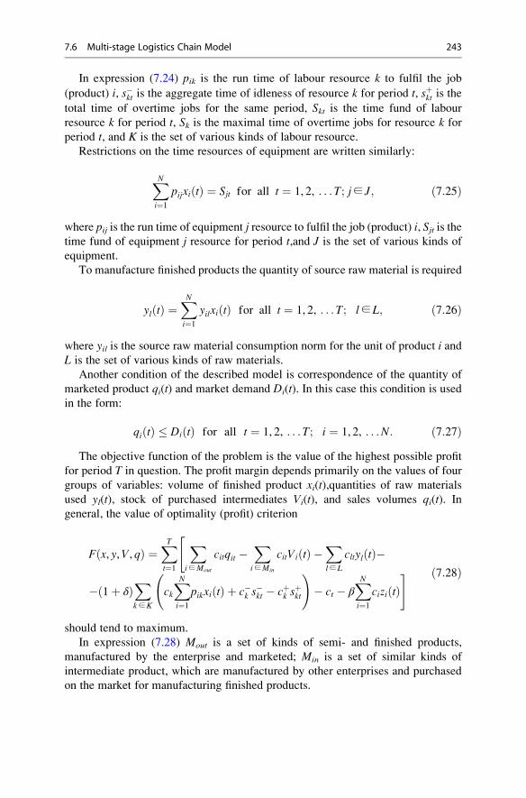
In expression (7.24) pik is the run time of labour resource k to fulfil the job
(product) i, s�kt is the aggregate time of idleness of resource k for period t, sþkt is thetotal time of overtime jobs for the same period, Skt is the time fund of labour
resource k for period t, Sk is the maximal time of overtime jobs for resource k for
period t, and K is the set of various kinds of labour resource.
Restrictions on the time resources of equipment are written similarly:
XNi¼1
pijxi tð Þ ¼ Sjt for all t ¼ 1, 2, . . . T; j∈ J; ð7:25Þ
where pij is the run time of equipment j resource to fulfil the job (product) i, Sjt is thetime fund of equipment j resource for period t,and J is the set of various kinds of
equipment.
To manufacture finished products the quantity of source raw material is required
yl tð Þ ¼XNi¼1
yilxi tð Þ for all t ¼ 1, 2, . . . T; l∈L; ð7:26Þ
where yil is the source raw material consumption norm for the unit of product i andL is the set of various kinds of raw materials.
Another condition of the described model is correspondence of the quantity of
marketed product qi(t) and market demand Di(t). In this case this condition is used
in the form:
qi tð Þ � Di tð Þ for all t ¼ 1, 2, . . . T; i ¼ 1, 2, . . .N: ð7:27ÞThe objective function of the problem is the value of the highest possible profit
for period T in question. The profit margin depends primarily on the values of four
groups of variables: volume of finished product xi(t),quantities of raw materials
used yl(t), stock of purchased intermediates Vi(t), and sales volumes qi(t). In
general, the value of optimality (profit) criterion
Fðx, y,V, qÞ ¼XTt¼1
" Xi∈Mout
citqit �Xi∈Min
citViðtÞ �Xl∈ L
cltylðtÞ�
�ð1þ δÞXk∈K
ckXNi¼1
pikxiðtÞ þ c�k s�kt � cþk s
þkt
!� ct � β
XNi¼1
ciziðtÞ# ð7:28Þ
should tend to maximum.
In expression (7.28) Mout is a set of kinds of semi- and finished products,
manufactured by the enterprise and marketed; Min is a set of similar kinds of
intermediate product, which are manufactured by other enterprises and purchased
on the market for manufacturing finished products.
7.6 Multi-stage Logistics Chain Model 243

Other designations in expression (7.28): cit—product price, clt—raw material
price, δ—unified social tax fee, ck—rate per time unit of labour resource job, c�k and
cþk —payment per time unit of idleness and extra payment for overtime job, ct—constant expenditures including depreciation, β—alternative return on assets for
one period t, and ci—i-type product cost.To achieve the maximum of function (7.28) it is necessary to vary the values of
variables xi(t), yl(t), Vi(t), and qi(t), including the constraints (Eqs. 7.22–7.27). In
fact, the set objective is the same as the problem of sales and operations scheduling,
which is discussed below in Chap. 10.
References
Ierapetritou, M. G., & Floudas, C. A. (1998). Effective continuous-time formulation for short-termscheduling. 1. Multipurpose batch processes. titan.princeton.edu/papers/marianthi/iera_
floudas_98a.pdf
Kestner, W., Blecker, T., & Herstatt, C. (2008). Innovative logistics management. Berlin: Schmidt
Erich.
Kondili, E., Pantelides, C. C., & Sargent, R. A. (1993). General algorithm for short-term schedul-
ing of batch operations. Computers and Chemical Engineering, 17, 211–227.Li, Z., & Ierapetritou, M. G. (2009). Integrated production planning and scheduling using a
decomposition framework. sol.rutgers.edu/staff/marianth/integratePS.pdf
Macedo, J. (2000). Implementing fast innovation reinforcement supply chains. www.iamot.org/
conference/index.php/ocs/9/paper/view/1957/926
Mauergauz, Y. (2007). Computer aided operative planning in mechanical engineering. Moscow:
Economics (in Russian).
Pleshchinsky, A. S. (2004). Optimization of intercompany interactions and intracompany man-agement solutions. Moscow: Nauka (in Russian).
Pleshchinsky, A. S., Pachkovsky, E. M., & Mikhailina, I. M. (2008). Coordinated optimization oflogistics, production and financial performance of multi-stage enterprises. Moscow: Central
Economic and Mathematical Institute of the RAS (in Russian).
Prilutsky, M. K., & Vlasov, S. E. (2007). Multi-stage problems of scheduling theory with alterna-tive variants of job performance. iani.unn.ru/assets/files/priluckiy_mh/mnogostad_teoriya_
raspisanii.doc (in Russian).
Rodnikov, A. N. (1995). Logistics. Dictionary of terms. Moscow: Ekonomika (in Russian).
Stadtler, H., & Kilger, C. (2008). Supply chain management and advanced planning. Concepts,models, software, and case studies (4th ed.). Berlin: Springer.
244 7 Examples of Advanced Planning Models

Part II
Planning Processes

Single-Echelon Inventory Planning 8
8.1 Inventory Types and Parameters
This chapter discusses the stocks, their characteristics, and methods of stock
planning. Stocks are generally classified (Grigoriev et al. 2007) by their intended
purpose and economic and logistical functions. From the planner’s point of view,
the main interest is in the division of all stocks into parts by functions in the
logistics process as follows:
• Current;
• Safety;
• Preparatory;
• Seasonal.
Preparatory stocks are for special preparation or incoming inspection prior to the
production process—for example, wood drying, quality assurance laboratory tests,
etc. The basis for the stocks calculation is demand values defined by the methods
discussed above in Chap. 6.
For stocks the so-called ABC classification into three categories is widely used.
Category A includes the most valuable goods comprising 20 % of stocks and
providing 80 % of sales. Category B includes 30 % of stocks, which give 15 % of
sales; category C is the least valuable goods comprising 50 % of stocks, giving 5 %
of sales.
Stock changes over time are characterized by a number of parameters influencing
the quantity of the individual parts of the stock. Let us consider the stock graph in the
simplest case (Fig. 8.1), when the demand is constant, the stock is replenished
instantaneously, and delivery is performed within a specified time interval.
In this case, the stock decreases from the highest value _S to the lowest
permissible Zc at a rate determined by demand value D. At time T of reaching the
# Springer International Publishing Switzerland 2016
Y. Mauergauz, Advanced Planning and Scheduling in Manufacturing and SupplyChains, DOI 10.1007/978-3-319-27523-9_8
247
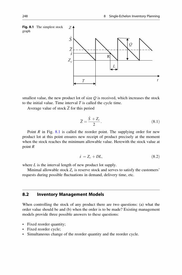
smallest value, the new product lot of size Q is received, which increases the stock
to the initial value. Time interval T is called the cycle time.
Average value of stock Z for this period
Z ¼_S þ Zc
2: ð8:1Þ
Point R in Fig. 8.1 is called the reorder point. The supplying order for new
product lot at this point ensures new receipt of product precisely at the moment
when the stock reaches the minimum allowable value. Herewith the stock value at
point R
_s ¼ Zc þ DL; ð8:2Þwhere L is the interval length of new product lot supply.
Minimal allowable stock Zc is reserve stock and serves to satisfy the customers’
requests during possible fluctuations in demand, delivery time, etc.
8.2 Inventory Management Models
When controlling the stock of any product there are two questions: (a) what the
order value should be and (b) when the order is to be made? Existing management
models provide three possible answers to these questions:
• Fixed reorder quantity;
• Fixed reorder cycle;
• Simultaneous change of the reorder quantity and the reorder cycle.
RcZsZ
t
Q
T
S
Z
L
.
.
Fig. 8.1 The simplest stock
graph
248 8 Single-Echelon Inventory Planning
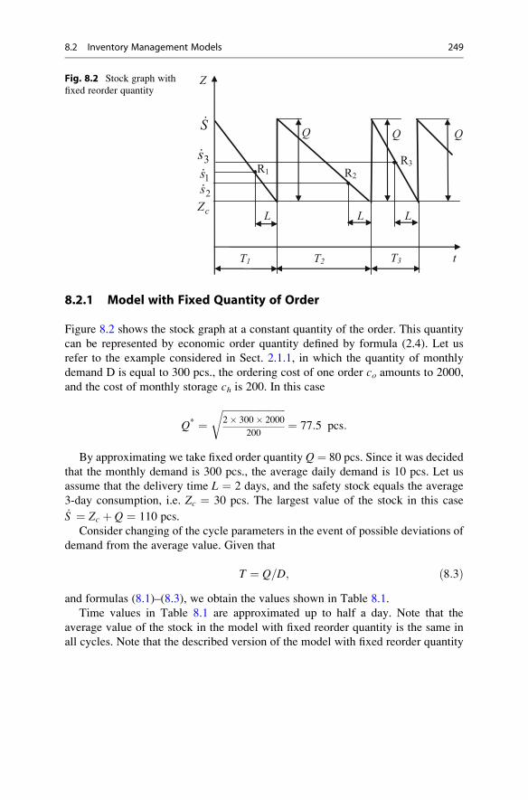
8.2.1 Model with Fixed Quantity of Order
Figure 8.2 shows the stock graph at a constant quantity of the order. This quantity
can be represented by economic order quantity defined by formula (2.4). Let us
refer to the example considered in Sect. 2.1.1, in which the quantity of monthly
demand D is equal to 300 pcs., the ordering cost of one order co amounts to 2000,
and the cost of monthly storage ch is 200. In this case
Q* ¼ffiffiffiffiffiffiffiffiffiffiffiffiffiffiffiffiffiffiffiffiffiffiffiffiffi2� 300� 2000
200
r¼ 77:5 pcs:
By approximating we take fixed order quantity Q ¼ 80 pcs. Since it was decided
that the monthly demand is 300 pcs., the average daily demand is 10 pcs. Let us
assume that the delivery time L ¼ 2 days, and the safety stock equals the average
3-day consumption, i.e. Zc ¼ 30 pcs. The largest value of the stock in this case_S ¼ Zc þ Q ¼ 110 pcs.
Consider changing of the cycle parameters in the event of possible deviations of
demand from the average value. Given that
T ¼ Q=D; ð8:3Þand formulas (8.1)–(8.3), we obtain the values shown in Table 8.1.
Time values in Table 8.1 are approximated up to half a day. Note that the
average value of the stock in the model with fixed reorder quantity is the same in
all cycles. Note that the described version of the model with fixed reorder quantity
R3R1
3s
L L
R2
cZ
t
Q
T1
S
Z
L
T2 T3
2s1s
.
.
.
.
Fig. 8.2 Stock graph with
fixed reorder quantity
8.2 Inventory Management Models 249
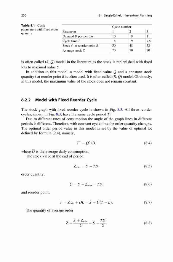
is often called (S, Q) model in the literature as the stock is replenished with fixed
lots to maximal value _S .In addition to this model, a model with fixed value Q and a constant stock
quantity _s at reorder point R is often used. It is often called (R,Q) model. Obviously,
in this model, the maximum value of the stock does not remain constant.
8.2.2 Model with Fixed Reorder Cycle
The stock graph with fixed reorder cycle is shown in Fig. 8.3. All three reorder
cycles, shown in Fig. 8.3, have the same cycle period T.Due to different rates of consumption the angle of the graph lines in different
periods is different. Therefore, with constant cycle time the order quantity changes.
The optimal order period value in this model is set by the value of optimal lot
defined by formula (2.4), namely,
T* ¼ Q*=D; ð8:4Þwhere D is the average daily consumption.
The stock value at the end of period:
Zmin ¼ _S � TD; ð8:5Þorder quantity,
Q ¼ _S � Zmin ¼ TD; ð8:6Þand reorder point,
_s ¼ Zmin þ DL ¼ _S � D T � Lð Þ: ð8:7ÞThe quantity of average order
Z ¼_S þ Zmin
2¼ _S � TD
2: ð8:8Þ
Table 8.1 Cycle
parameters with fixed order
quantityParameter
Cycle number
1 2 3
Demand D pcs per day 10 9 11
Cycle time T 8 9 7.5
Stock _s: at reorder point R 50 48 52
Average stock Z 70 70 70
250 8 Single-Echelon Inventory Planning
For the example, considered in the previous paragraph, optimal period value
T ¼ 80/10 ¼ 8 days. Assume that the highest proffered quantity of order is as
previously _S ¼ 110 pcs.
The changes in the cycle parameters for possible deviations in demand from the
average value in this case are presented in Table 8.2.
As can be seen from Table 8.2, in this model the value of average stock increases
with the decrease of demand. The model with fixed reorder cycle and fixed maximal
stock value is called (S, T ) model.
8.2.3 Two-Tier Inventory Management Model
This model establishes two levels of stock: maximal required stock _S and the level
defining the reorder point _s . The order is made as soon as the actual value of the
stock reaches level _s in order to replenish the stock up to level _S .Figure 8.4 shows the stock graph in this model. In this case, if the demand varies,
both the reorder cycle and the order quantities vary. The reorder cycle as shown in
Fig. 8.4:
T ¼ _S � _s�
=Dþ L; ð8:9Þorder quantity
Q ¼ _S � _s þ DL; ð8:10Þstock at the end of period
Q3Q1
R3
R1
3s
L L
R2
cZ
1s
t
Q2
T
Z
L
T T
2s
S.
.
.
.
Fig. 8.3 Stock graph with
fixed reorder cycle
8.2 Inventory Management Models 251

Zmin ¼ _S � Q;
and average value of stock for a cycle
Z ¼_S þ Zmin
2¼
_S þ _s � DL
2: ð8:11Þ
Returning to the above discussed example, where safety stock Zc ¼ 30 pcs., the
maximal allowable stock _S ¼ 110 pcs., delivery time L¼ 2 days, and average value
of consumption D ¼ 10 pcs./day, let us define reorder point _s from expression (8.2)
_s ¼ Zc þ DL ¼ 30þ 10� 2 ¼ 50 pcs:
The cycle parameters for possible deviations in demand from the average value
in this case are presented in Table 8.3.
In literature the two-tier model is often referred as (s, S) model or a threshold
model, because value _s is threshold (trigger) point of reorder, and the highest value
of stock _S is fixed.
Table 8.2 Cycle
parameters with fixed
reorder cycleParameter
Cycle number
1 2 3
Demand D pcs per day 10 9 11
Cycle time T 80 72 88
Stock _s in reorder point R 50 56 44
Average stock Z 70 74 66
T2
Q3Q1
R3R1
L L
R2
cZ
s
t
Q2
T
Z
L
T3
S.
.
Fig. 8.4 Stock graph with
two-tier model
252 8 Single-Echelon Inventory Planning

8.2.4 Benchmarking of Inventory Management Models
The simplest model is a fixed reorder cycle model. This model is common among
small businesses (shops), the procurement of which is done quickly and regularly
from sustainable suppliers. In this case, the order quantity is usually determined
manually considering the current consumption and the forecast for the next period.
Comparing the data in Tables 8.1–8.3, we see that with fixed reorder cycle
(Table 8.2), even with small fluctuations in demand, there are significant changes
in both the order size and the average stock value.
The fixed reorder quantity model is used when the possible value changes with a
big step—by the amount of product per pallet, container, tank, etc. In these cases, at
small variation in demand the changes in order quantities are undesirable. Further-
more, this model is usually used if the product which is consumed in small amounts
has the so-called transit rate—minimum quantity shipped to one consignee. Where
there is the transit rate of the order quantity is forced to coincide with the value of
this rate.
From Table 8.1, it is clear that even a slight reduction in demand in this model
leads to a significant increase in the cycle time that is fraught with the possibility of
obsolescence of a long stored product. The moment of order in the fixed reorder
quantity model is usually determined manually.
Unlike the first two models, the two-tier model is well suited for automatic
reorder and therefore widely used in automated stock management systems. The
analysis of Table 8.3 shows that here small variations in demand lead to slight
deviation of the order quantity, cycle time, and the average stock value.
It should be noted that the two-tier model allows two possibilities of reorder
launch: (a) when the stock value becomes equal to value _s: and (b) when the stock
value is less than _s: by one unit. The difference between these variants is important
in those cases where the value of demand is low and the stock changes slowly,
especially at small quantity of the safety stock.
Since the product is normally consumed by portions, the amount of stock rarely
coincides exactly with threshold value _s . Therefore, the most common rule of
reorder launch is condition
Z � _s ; ð8:12Þi.e. to perform this launch it is necessary that the current value becomes equal or
less than threshold _s .
Table 8.3 Cycle
parameters with two-tier
modelParameter
Cycle number
1 2 3
Demand D pcs per day 10 9 11
Order quantity Q 80 78 82
Cycle time T 8 8.5 7.5
Average stock Z 70 71 69
8.2 Inventory Management Models 253
When determining the current value of the stock, it is necessary to take into
account the stock in transit. The value of this stock depends on delivery duration L.If L � T, i.e. the delivery duration is less than or equal to the cycle of stock
fluctuations, then one product lot should be in transit; otherwise the number of
lots in transit can be several. The above stock models are for the first case as a rule.
In the two-tier model, the order is often approximated to a quantity of a number
of allowable values. With small fluctuations in demand in such cases the quantity of
the order is simply equal to the optimal fixed value. However, with such approxi-
mation the stock after another receipt should not exceed the volume (area) of its
storage container.
8.2.5 Kanban Inventory Management Model
Currently system Kanban has become widely known. It is usually defined as a
system of “pulling” products from the previous echelon of production. In terms of
models outlined above, system Kanban is some kind of two-tier model, which uses
fixed reorder quantity (Axseter 2006).
This system’s information medium is the turnover mechanism of cards (kanbans)
of two kinds used for production management. The information in the cards of
the first type—withdrawal kanbans—describes the number of objects that must be
delivered to the place of consumption. In the second type of cards—production-
ordering kanbans—the number of products, which must be made at the production
site, are recorded. Figure 8.5 shows the diagram of kanban circulation between two
echelons of the production process—machines 1 and 2.
Besides machines 1 and 2, the diagram shows two buffers (storages) B1 and B2
of cards exchange. In buffer B1, the selection card that has come with empty
container is replaced by the order card, which then together with this container
is sent to machine 1. The withdrawal kanban from buffer B1 is transferred to
B2. Container 1 with the product of machine 1, accompanied by the production-
ordering kanban, goes into B2 too. In B2 on this container the production-ordering
kanban is replaced by a withdrawal kanban and then the container is transferred for
processing on machine 2.
Replacement of the withdrawal kanban by ordering kanban happens every time
after another container that is fed to machine 2 becomes empty. Since the capacity
of all containers is the same, the order quantity Q is equal to the capacity. The stock
value at reorder point _s is also constant and equal to the product quantity in all
containers in transit from machine 1 to machine 2. This amount is determined by
demand value D and cycle time L for delivery of product produced on machine 1 to
machine 2. In addition, the need for the safety stock should be taken into account.
Thus, the stock at the reorder point
_s ¼ DLþ Zc: ð8:13Þ
254 8 Single-Echelon Inventory Planning
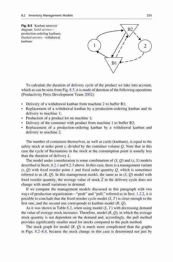
To calculate the duration of delivery cycle of the product we take into account,
which as can be seen from Fig. 8.5, it is made of duration of the following operations
(Productivity Press Development Team 2002):
• Delivery of a withdrawal kanban from machine 2 to buffer B1;
• Replacement of a withdrawal kanban by a production-ordering kanban and its
delivery to machine 1;
• Production of a product lot on machine 1;
• Delivery of the container with product from machine 1 to buffer B2;
• Replacement of a production-ordering kanban by a withdrawal kanban and
delivery to machine 2.
The number of containers themselves, as well as cards (kanbans), is equal to the
safety stock at order point s, divided by the container volume Q. Note that in this
case the cycle of fluctuations in the stock at the consumption point is usually less
than the duration of delivery L.The model under consideration is some combination of (S, Q) and (s, S) models
described in Sects. 8.2.1 and 8.2.3 above. In this case, there is a management variant
(s, Q) with fixed reorder point _s and fixed order quantity Q, which is sometimes
referred to as (R, Q). In this management model, the same as in (S, Q) model with
fixed reorder quantity, the average value of stock Z in the delivery cycle does not
change with small variations in demand.
If we compare the management models discussed in this paragraph with two
ways of production organization—“push” and “pull,” referred to in Sect. 1.2.2, it is
possible to conclude that the fixed reorder cycle model (S, T ) is close enough to thefirst one, and the second one corresponds to kanban model (R, Q).
As it was shown in Table 8.2, when using model (S, T ) with decreasing demand
the value of average stock increases. Therefore, model (R, Q), in which the averagestock quantity is not dependent on the demand and, accordingly, the pull method
provides significantly smaller need for stocks compared to the push method.
The stock graph for model (R, Q) is much more complicated than the graphs
in Figs. 8.2–8.4, because the stock change in this case is determined not just by
1 2
B1
B2Fig. 8.5 Kanban turnover
diagram. Solid arrows—production-ordering kanbans;
Dashed arrows—withdrawal
kanbans
8.2 Inventory Management Models 255
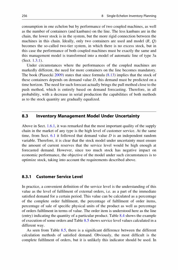
consumption in one echelon but by performance of two coupled machines, as well
as the number of containers (and kanbans) on the line. The less kanbans are in the
chain, the lower stock is in the system, but the more rigid connection between the
machines in this chain. Ideally, only two containers are used and model (R, Q)becomes the so-called two-tier system, in which there is no excess stock, but in
this case the performance of both coupled machines must be exactly the same and
this management model is transformed into a model of automatic line of type 3a
(Sect. 1.3.1).
Under circumstances where the performances of the coupled machines are
markedly different, the need for more containers on the line becomes mandatory.
The book (Piasecki 2009) states that since formula (8.13) implies that the stock of
these containers depends on demand value D, this demand must be predicted on a
time horizon. The need for such forecast actually brings the pull method close to the
push method, which is entirely based on demand forecasting. Therefore, in all
probability, with a decrease in serial production the capabilities of both methods
as to the stock quantity are gradually equalized.
8.3 Inventory Management Model Under Uncertainty
Above in Sect. 1.6.1, it was remarked that the most important quality of the supply
chain in the market of any type is the high level of customer service. At the same
time, from Sect. 6.1 it followed that demand value D is an independent random
variable. Therefore, it is clear that the stock model under uncertainty must ensure
the amount of current reserves that the service level would be high enough at
forecasted demand. However, since too much stock has negative impact on
economic performance, the objective of the model under such circumstances is to
optimize stock, taking into account the requirements described above.
8.3.1 Customer Service Level
In practice, a convenient definition of the service level is the understanding of this
value as the level of fulfilment of external orders, i.e. as a part of the immediate
satisfied demand for a certain period. This value can be calculated as a percentage
of the complete order fulfilment, the percentage of fulfilment of order items,
percentage of sale of specific physical units of the product as well as percentage
of orders fulfilment in terms of value. The order item is understood here as the line
(entry) indicating the quantity of a particular product. Table 8.4 shows the example
of execution of some orders and Table 8.5 shows service level values calculated in a
different way.
As seen from Table 8.5, there is a significant difference between the different
calculation methods of satisfied demand. Obviously, the most difficult is the
complete fulfilment of orders, but it is unlikely this indicator should be used. In
256 8 Single-Echelon Inventory Planning
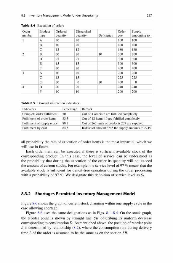
all probability the rate of execution of order items is the most impartial, which we
will use in future.
Each order item can be executed if there is sufficient available stock of the
corresponding product. In this case, the level of service can be understood as
the probability that during the execution of the order its quantity will not exceed
the amount of current stocks. For example, the service level of 97 % means that the
available stock is sufficient for deficit-free operation during the order processing
with a probability of 97 %. We designate this definition of service level as SL.
8.3.2 Shortages Permitted Inventory Management Model
Figure 8.6 shows the graph of current stock changing within one supply cycle in the
case allowing shortage.
Figure 8.6 uses the same designations as in Figs. 8.1–8.4. On the stock graph,
the reorder point is shown by straight line _SR describing its uniform decrease
corresponding to consumption D. As mentioned above, the position of reorder point
_s is determined by relationship (8.2), where the consumption rate during delivery
time L of the order is assumed to be the same as on the section _SR.
Table 8.4 Execution of orders
Order
number
Product
type
Ordered
quantity
Dispatched
quantity Deficiency
Order
cost
Supply
amounting to
1 A 20 20 100 100
B 40 40 400 400
C 12 12 180 180
2 B 30 20 10 300 200
D 25 25 300 300
E 15 15 300 300
F 20 20 400 400
3 A 40 40 200 200
C 15 15 225 225
E 20 0 20 400 0
4 D 20 20 240 240
F 10 10 200 200
Table 8.5 Demand satisfaction indicators
Indicators Percentage Remark
Complete order fulfilment 50 Out of 4 orders 2 are fulfilled completely
Fulfilment of order items 83.3 Out of 12 items 10 are fulfilled completely
Fulfilment of supply scope 88.7 Out of 267 units of products 237 are supplied
Fulfilment by cost 84.5 Instead of amount 3245 the supply amounts to 2745
8.3 Inventory Management Model Under Uncertainty 257
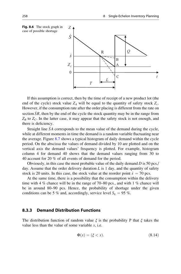
If this assumption is correct, then by the time of receipt of a new product lot (the
end of the cycle) stock value ZA will be equal to the quantity of safety stock Zc.However, if the consumption rate after the order placing is different from the rate on
section _SR, then by the end of the cycle the stock quantity may be in the range from
ZB to ZC. In the latter case, it may appear that the safety stock is not enough, and
there is deficiency.
Straight line _SA corresponds to the mean value of the demand during the cycle,
while at different moments in time the demand is a random variable fluctuating near
the average. Figure 8.7 shows a typical histogram of daily demand within the cycle
period. On the abscissa the values of demand divided by 10 are plotted and on the
vertical axis the demand values’ frequency is plotted. For example, histogram
column 4 for demand 40 shows that the demand values ranging from 30 to
40 account for 20 % of all events of demand for the period.
Obviously, in this case the most probable value of the daily demand D is 50 pcs./
day. Assume that the order delivery duration L is 1 day, and the quantity of safety
stock is 20 units. In this case, the stock value at the reorder point _s ¼ 70 pcs.
At the same time, there is a possibility that the consumption within the delivery
time with 4 % chance will be in the range of 70–80 pcs., and with 1 % chance will
be in around 80–90 pcs. Hence, the probability of shortage under the given
conditions can be 5 % and, accordingly, service level SL ¼ 95 %.
8.3.3 Demand Distribution Functions
The distribution function of random value ξ is the probability Ρ that ξ takes the
value less than the value of some variable x, i.e.
Φ xð Þ ¼ ξ < xð Þ: ð8:14Þ
A
QR
L
cZ
s
tT
Z
0
B
C
S.
.
Fig. 8.6 The stock graph in
case of possible shortage
258 8 Single-Echelon Inventory Planning
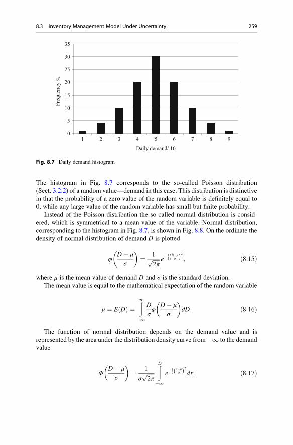
The histogram in Fig. 8.7 corresponds to the so-called Poisson distribution
(Sect. 3.2.2) of a random value—demand in this case. This distribution is distinctive
in that the probability of a zero value of the random variable is definitely equal to
0, while any large value of the random variable has small but finite probability.
Instead of the Poisson distribution the so-called normal distribution is consid-
ered, which is symmetrical to a mean value of the variable. Normal distribution,
corresponding to the histogram in Fig. 8.7, is shown in Fig. 8.8. On the ordinate the
density of normal distribution of demand D is plotted
φD� μ
σ
� �¼ 1ffiffiffiffiffi
2πp e�
12
D�μσð Þ2 ; ð8:15Þ
where μ is the mean value of demand D and σ is the standard deviation.
The mean value is equal to the mathematical expectation of the random variable
μ ¼ E Dð Þ ¼ð1
�1
D
σφ
D� μ
σ
� �dD: ð8:16Þ
The function of normal distribution depends on the demand value and is
represented by the area under the distribution density curve from�1 to the demand
value
ΦD� μ
σ
� �¼ 1
σffiffiffiffiffi2π
pðD
�1e�
12
x�μσð Þ2dx: ð8:17Þ
0
5
10
15
20
25
30
35
1 2 3 4 5 6 7 8 9
Fre
qu
ency
%
Daily demand/ 10
Fig. 8.7 Daily demand histogram
8.3 Inventory Management Model Under Uncertainty 259
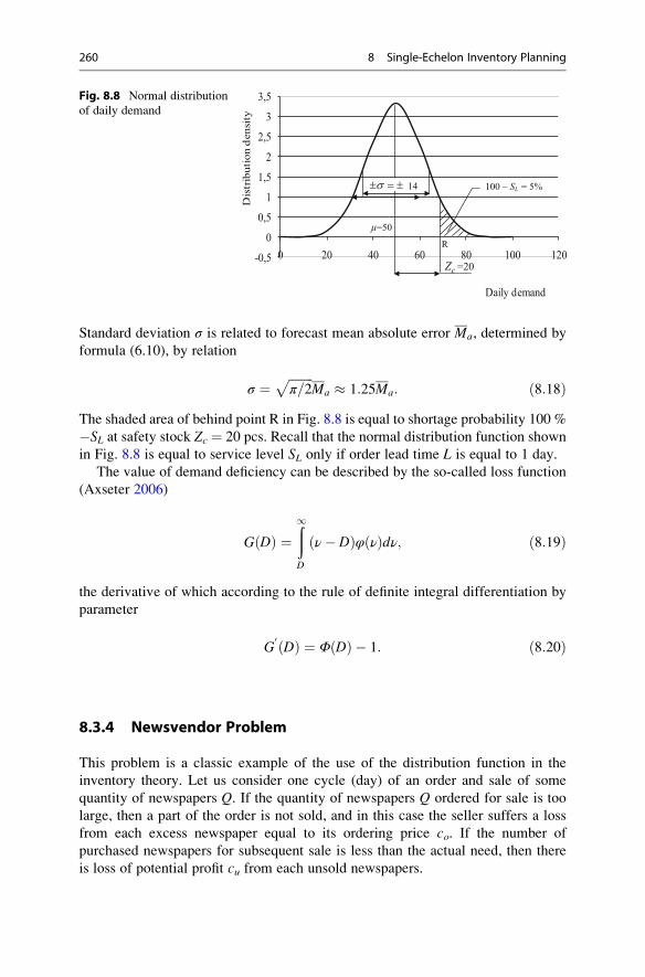
Standard deviation σ is related to forecast mean absolute error Ma, determined by
formula (6.10), by relation
σ ¼ffiffiffiffiffiffiffiffiπ=2
pMa � 1:25Ma: ð8:18Þ
The shaded area of behind point R in Fig. 8.8 is equal to shortage probability 100 %
�SL at safety stock Zc ¼ 20 pcs. Recall that the normal distribution function shown
in Fig. 8.8 is equal to service level SL only if order lead time L is equal to 1 day.
The value of demand deficiency can be described by the so-called loss function
(Axseter 2006)
G Dð Þ ¼ð1D
ν� Dð Þφ νð Þdν; ð8:19Þ
the derivative of which according to the rule of definite integral differentiation by
parameter
G0Dð Þ ¼ Φ Dð Þ � 1: ð8:20Þ
8.3.4 Newsvendor Problem
This problem is a classic example of the use of the distribution function in the
inventory theory. Let us consider one cycle (day) of an order and sale of some
quantity of newspapers Q. If the quantity of newspapers Q ordered for sale is too
large, then a part of the order is not sold, and in this case the seller suffers a loss
from each excess newspaper equal to its ordering price co. If the number of
purchased newspapers for subsequent sale is less than the actual need, then there
is loss of potential profit cu from each unsold newspapers.
-0,5
0
0,5
1
1,5
2
2,5
3
3,5
0 20 40 60 80 100 120D
istr
ibuti
on d
ensi
ty
Daily demand
μ=50
σ± = ± 14
cZ =20
100 – SL = 5%
R
Fig. 8.8 Normal distribution
of daily demand
260 8 Single-Echelon Inventory Planning

Considering that demand D is a random variable with mean value μ and standarddeviation σ, we define value Q, at which vendor’s loss c(D) is minimal. To do this,
we note that
c Dð Þ ¼ Q� Dð Þco at D < Qand
c Dð Þ ¼ D� Qð Þcu at D > Q:ð8:21Þ
Considering that demand is a random function with distribution density φ D�μσ
� ,
the total losses of the vendor can be defined as the mathematical expectation of loss
amount (formula 8.21), i.e. c ¼ E c Dð Þ½ � or
c ¼ co
ðQ�1
Q� D
σφ
D� μ
σ
� �dDþ cu
ð1Q
D� Qð Þσ
φD� μ
σ
� �dD: ð8:22Þ
Using expression (8.16), we have
c ¼ co Q� μð Þ þ co þ cuð Þð1Q
D� Qð Þσ
φD� μ
σ
� �dD ð8:23Þ
and taking into account (formula 8.19), we obtain
c ¼ co Q� μð Þ þ co þ cuð ÞσG D� μ
σ
� �: ð8:24Þ
To define the minimal value of losses, we take the derivative and using formula
(8.20) we obtain the following equation:
dc
dQ¼ co þ co þ cuð Þ Φ
Q� μ
σ
� �� 1
�¼ 0; ð8:25Þ
from which we find the solution of the problem in the form
ΦQ� μ
σ
� �¼ cu
co þ cu: ð8:26Þ
As an example, consider the case, in which the purchase price co ¼ 10, the sales
up-lift cu ¼ 15, and daily demand distribution correspond to the graph in Fig. 8.8.
We have
8.3 Inventory Management Model Under Uncertainty 261

ΦQ� 50
14
� �¼ 15
10þ 15¼ 0:625:
To define the optimal value of order quantity Q, we use integral function
NORMDIST from MS Excel, selecting integral values Q so that the value of
function NORMDIST Q�5014
� is as close as possible to 0.625. This value (0.639)
is Q¼ 55. As you can see, the optimal quantity of the order in this case is somewhat
higher than the mean value of demand.
The problems similar to those described are often found when ordering various
perishable or rapidly obsolescent products.
8.4 Inventory Management Using Logistic Operating Curves
Storage Operating Curves method can be used to define the optimal stock level as
well as to account the supply deviations’ influence on the capability to provide
service.
8.4.1 Storage Curves and Their Applications
A model of logistic chain of the procurement process can be represented by a
diagram of stock movement at the storage similar to the diagram of processing time
flow in manufacturing above in Sect. 3.2.1 in Fig. 3.6. In this case, the steps in the
diagram are determined by the values of receipt and withdrawal from the storage.
The current stock is equal to the vertical segment between the curves of receipt and
withdrawal, and the horizontal line between these curves represents time spent in
the storage.
The dilemma of operational planning for the case of storage management
described above in Sect. 3.2 is to find a balance between high level of customer
service and low value of stocks. A measure of the service level may be a compli-
ance degree of the plan of requests fulfilment to receive from the storage and actual
values of goods or materials withdrawal, wherein the mean delivery delay for a
certain period may be determined as the sum of productions of the shortage quantity
per number of days of waiting. The dependence of mean delivery delay T on the
average value of stockZ for the period can be represented graphically in the form of
so-called storage operating curve.
In a similar way to the above logistics theory for production, the theory of
storage operating curve is based on a comparison of this curve with some ideal
curve. It is assumed that the withdrawal from the storage is uniform and in the same
quantities of some product. For such conditions (Nyhuis and Wiendahl 2009), it is
found that the relationship between T and Z is described by formula
262 8 Single-Echelon Inventory Planning
T ¼ Q=2�ffiffiffiffiffiffiffiffiffiffi2Q Z
pþ Z
D;ð8:27Þ
where Q is the average size of goods or material lot, received at the storage, and Dis the average rate of withdrawal of goods or material from the storage.
Function (8.27) equals 0 at
Z0 ¼ Q
2: ð8:28Þ
The second typical point of dependence (formula 8.27) is determined at Z ¼ 0
T0 ¼ Q
2D: ð8:29Þ
The family of curves, which includes both an ideal storage curve and the actual
curves, by analogy with the family of logistic operating curves can be described by
parametric dependencies
Z ¼ Z1 � t; T ¼ T1 �ffiffiffiffiffiffiffiffiffiffiffiffi1� tc
cp
at 0 � t � 1; ð8:30Þwhere value Z1 corresponds to the stock with zero delay with regard to necessary
safety stock and value T1 corresponds to the delay value at zero stocks and possible
deviations from the ideal conditions of supplies. For the case of the ideal curve,
degree indicator c equals 0.5; Z1 ¼ Z0; T1 ¼ T0.
The farther the actual storage curve is separated from the ideal, the greater, at the
set delay value, stocks must exist, which are necessary for customer service.
Modern production typically uses a very large range of materials and components
and, as a rule, it is impossible to hold stocks, immediately providing user requests,
for all items at the same time. Therefore, it is important to establish such quantities
of stocks for certain items that would ensure acceptable level of delays in actual
practice.
Since the entire set of storage items is usually divided into consumption groups
in accordance with the widely used ABC classification, then for each group it is
advisable to carry out logistical positioning, which is to determine the rational
operating point on the relevant storage curve. At the same time, the form of the
storage curve may vary for the same product depending on the nature of the
supplier’s activity.
Suppliers can also be divided into groups by the so-called UVW classification
based on the delays of shipments: group U includes suppliers with small delay,
group V—average delays values, and group W—with the values significantly
higher than the average ones. Assessment of the reliability of suppliers is probably
the most relevant for suppliers of W group. If some item is supplied by various
suppliers in parallel, then to evaluate their relative reliability it is possible to build
8.4 Inventory Management Using Logistic Operating Curves 263
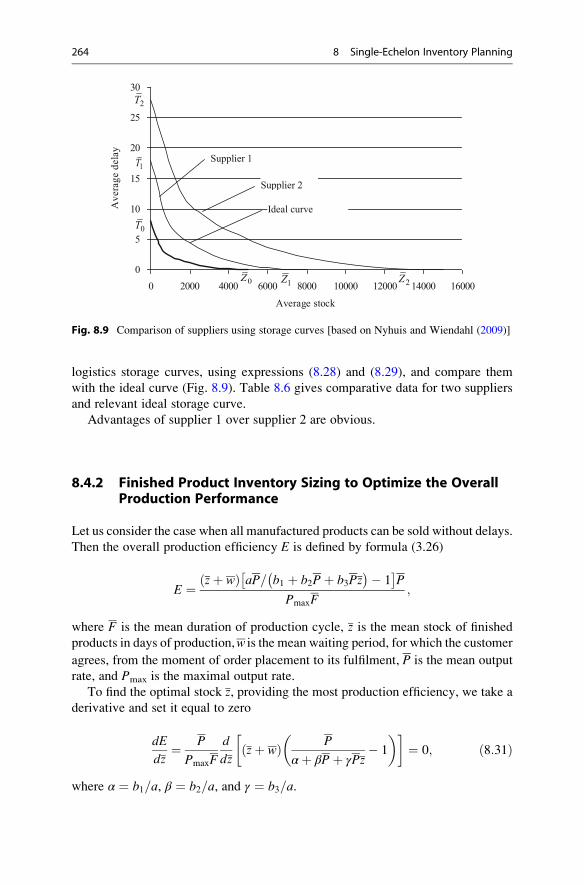
logistics storage curves, using expressions (8.28) and (8.29), and compare them
with the ideal curve (Fig. 8.9). Table 8.6 gives comparative data for two suppliers
and relevant ideal storage curve.
Advantages of supplier 1 over supplier 2 are obvious.
8.4.2 Finished Product Inventory Sizing to Optimize the OverallProduction Performance
Let us consider the case when all manufactured products can be sold without delays.
Then the overall production efficiency E is defined by formula (3.26)
E ¼ zþ wð Þ aP= b1 þ b2Pþ b3Pz� � 1
� P
PmaxF;
where F is the mean duration of production cycle, z is the mean stock of finished
products in days of production,w is the mean waiting period, for which the customer
agrees, from the moment of order placement to its fulfilment, P is the mean output
rate, and Pmax is the maximal output rate.
To find the optimal stock z, providing the most production efficiency, we take a
derivative and set it equal to zero
dE
dz¼ P
PmaxF
d
dzzþ wð Þ P
αþ βPþ γPz� 1
� � �¼ 0; ð8:31Þ
where α ¼ b1=a, β ¼ b2=a, and γ ¼ b3=a.
0
5
10
15
20
25
30
0 2000 4000 6000 8000 10000 14000 16000
Average stock
Av
erag
e d
elay
0TIdeal curve
Supplier 1
Supplier 2
1T
2T
0Z1Z 2Z
12000
Fig. 8.9 Comparison of suppliers using storage curves [based on Nyhuis and Wiendahl (2009)]
264 8 Single-Echelon Inventory Planning

By calculating the derivative in formula (8.31), using a number of algebraic
transformations we obtain for the optimal value of stock
Z* ¼ 1
γ
ffiffiffiffiffiffiffiffiffiffiffiffiffiffiffiffiffiffiffiffiffiffiffiα
Pþ β � γw
r� α
P� β
� �: ð8:32Þ
Figure 8.10 shows the graphs of optimum stock variation depending on the
allowable waiting period of customers at different output rates P, h/day. In this
example, we used the values of the coefficients from Sect. 3.3.3: a¼ 2000 unit/h,
b1 ¼ 350 thous. of units/day, b2 ¼ 500 unit/h, and b3 ¼ 50 unit/h/day.
As can be seen from Fig. 8.10, the optimal stock decreases with an increase
in the allowable waiting period and at some point becomes equal to 0. For it is
assumed that when output rate P is actually determined by the volume of sales, the
graphs indicate that the optimal quantity of the stock with an increase in sales
volume increases first and then stabilizes.
The optimal quantity of the stock depends on the values of input coefficients b1,b2, and b3 and profit margin a, and the decrease of the input coefficients or the
increase of profit margin leads to increase in the stock.
8.5 Safety Stock Sizing
Upper limit _S: of the storage stock, as it can be seen from Fig. 8.6 for example, is
determined as the sum of order quantity Q and the quantity of safety stock Zc. Theoptimal quantity of the order is calculated by the above formula (2.4), and the
calculation is discussed here below in Chap. 11.
In the inventory theory, mainly two approaches are used to determine the level
of safety stocks. The first of them (normative), using different rules, calculates
the level of stock, which should guarantee fully balanced operation. Several of
these rules are described in detail in Lukinsky (2007). The comparative analysis
of calculation by these rules, which was carried out in this paper, shows that the
results obtained in various ways are markedly different and, of course, hardly
actually ensure no shortage.
The more modern approach (stochastic) is that not the full absence of shortage
should be guaranteed but the set level of customer service, as described in Sect. 8.3.
Table 8.6 Comparative data of suppliers
Curve Minimal stock level Z1 The maximum delay of supply T1
Ideal 5000 pcs. 8 days
Supplier 1 8000 pcs. 18 days
Supplier 2 15,000 pcs. 28 days
8.5 Safety Stock Sizing 265
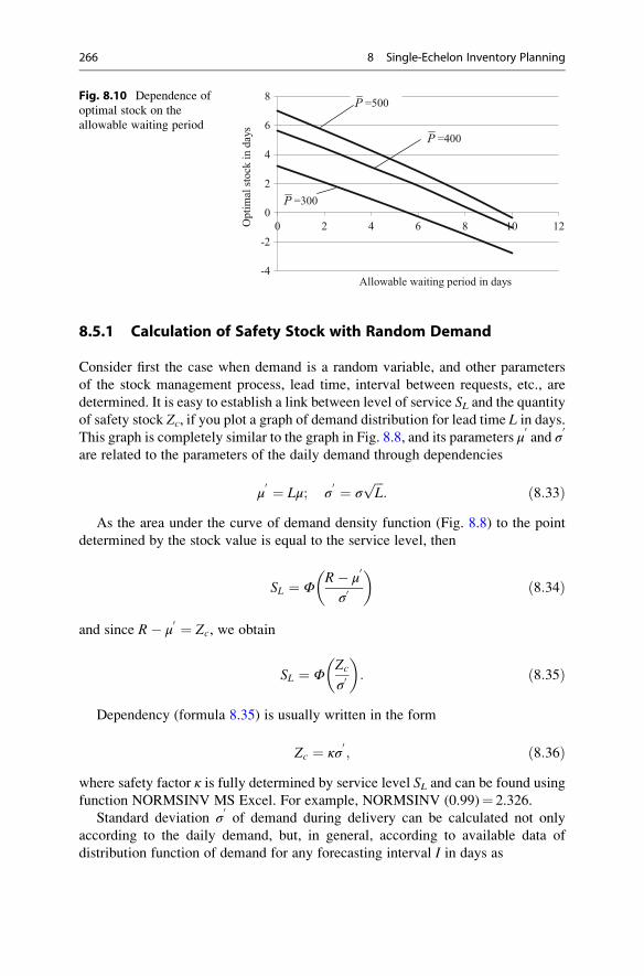
8.5.1 Calculation of Safety Stock with Random Demand
Consider first the case when demand is a random variable, and other parameters
of the stock management process, lead time, interval between requests, etc., are
determined. It is easy to establish a link between level of service SL and the quantityof safety stock Zc, if you plot a graph of demand distribution for lead time L in days.
This graph is completely similar to the graph in Fig. 8.8, and its parameters μ0and σ
0
are related to the parameters of the daily demand through dependencies
μ0 ¼ Lμ; σ
0 ¼ σffiffiffiL
p: ð8:33Þ
As the area under the curve of demand density function (Fig. 8.8) to the point
determined by the stock value is equal to the service level, then
SL ¼ ΦR� μ
0
σ0
� �ð8:34Þ
and since R� μ0 ¼ Zc, we obtain
SL ¼ ΦZc
σ0
� �: ð8:35Þ
Dependency (formula 8.35) is usually written in the form
Zc ¼ κσ0; ð8:36Þ
where safety factor κ is fully determined by service level SL and can be found usingfunction NORMSINV MS Excel. For example, NORMSINV (0.99)¼ 2.326.
Standard deviation σ0of demand during delivery can be calculated not only
according to the daily demand, but, in general, according to available data of
distribution function of demand for any forecasting interval I in days as
-4
-2
0
2
4
6
8
0 2 4 6 8 10 12Op
tim
al s
tock
in
day
s
Allowable waiting period in days
P =500
P =400
P =300
Fig. 8.10 Dependence of
optimal stock on the
allowable waiting period
266 8 Single-Echelon Inventory Planning
σ0 ¼ σ
ffiffiffiffiL
I:
rð8:37Þ
Let the lead time be L ¼ 2 days. To distribute the daily demand in Sect. 8.3.3
with σ ¼ 14 and service level SL ¼ 0.99, we obtain
Zc ¼ 2:326� 14ffiffiffi2
p� 46 pcs:
8.5.2 Sizing of Safety Stock with Two Random Variables
In fact, the process of stock management takes place under the conditions, where
not only the demand but also other process parameters are also random variables.
First, a random value is the order lead time. To calculate the quantity of safety stock
in this case it is natural to try to use formula (8.36), where we can try to determine
somehow the value of standard deviation σ0regarding the influence of random
variable L.The simplest option of such integration is described, for example, in Vollmann
et al. (2005) as the function
σ0 ¼
ffiffiffiffiffiffiffiffiffiffiffiffiffiffiffiffiffiffiffiffiffiffiDσ2D þ Lσ2L
q; ð8:38Þ
where D is the mean demand, units/days; L is the mean lead time in days; σD is
standard deviation of demand in units; and σL is standard deviation of lead time in
days. It is obvious that components under the radical sign in expression (8.38) have
different dimensions, but, oddly enough, recognizing this fact, the authors of the
book (Vollmann et al. 2005) continue using this expression.
More famous is the option of the joint account for deviations in demand and lead
time in the form
σ0 ¼
ffiffiffiffiffiffiffiffiffiffiffiffiffiffiffiffiffiffiffiffiffiffiffiffiLσ2D þ D
2σ2L
q: ð8:39Þ
In this expression, as in the previous one, the components under the radical sign
also have different dimensions. This fact clearly indicates the impossibility of its
use. In the book (Grigoriev et al. 2007), the following relationship is proposed in
order to close the dimensions gap:
σ0 ¼
ffiffiffiffiffiffiffiffiffiffiffiffiffiffiffiffiffiffiffiffiffiffiffiffiffiffiL2σ2D þ D
2σ2L
q; ð8:40Þ
however, as shown in (Lukinsky 2007), this expression is valid only if the demand-
time dependence is linear.
8.5 Safety Stock Sizing 267
In our opinion, it seems unacceptable to use the dependence like (formulas 8.38–
8.40), at least as long as the experts in the field of probability theory do not find out
about the origin of the paradox. In the current situation, we can suggest to use semi-
empirical approach based on a number of theoretical and experimental data on the
use of dependencies (formulas 8.36 and 8.37).
First of all, in Axseter (2006) it is indicated that dependence (formula 8.37) is
satisfied exactly if the values of demand standard deviation σ in different time
periods are independent. Since this is often not the case, then theoretically, instead
of formula (8.37), we should use a more general dependency
σ0 ¼ σ
L
I
� �c
; ð8:41Þ
where index 0:5 � c � 1. Value c ¼ 0:5 corresponds to the independence of
demand values in different time periods, value c ¼ 1—the case of full correlation,
and actual value c should be between 0.5 and 1.
In the paper of Rosenfield (1994), extensive experimental data were obtained
to determine the dependence of the demand standard deviation on the mean lead
time L and the mean value of demand D for consumer goods. It turned out that this
dependence is well described by expression
σT,D ¼ aD0:7L0:7; ð8:42Þ
where a is the coefficient determined for each specific item of goods. To calculate
value a, it is necessary to obtain the value of the standard deviation by experiment
with known and constant values of D and L.To reconcile the result (formula 8.42) with dependence (formula 8.41), we
introduce the concept of the basic forecasting interval. We take the most convenient
for observation time interval for this basic interval for assessing the demand
distribution. For example, as in construction of histogram (formula 8.7), it is most
convenient to define the parameters of daily demand; the basic forecasting interval
here is obviously 1 day.
We denote the value of mean demand D on the basic interval through μ and the
value of the standard deviation through σ. Then, by analogy with expressions (8.41)and (8.42) we can write
σ0 ¼ σ
D
μ
� �0:7L
I
� �0:7
ð8:43Þ
and
Zc ¼ κσ0: ð8:44Þ
268 8 Single-Echelon Inventory Planning
From formula (8.43), it follows that with D ¼ μ and L ¼ I, deviation σ0automati-
cally becomes equal to σ. If D ¼ μ, and L 6¼ I, then (formula 8.43) turns into
(formula 8.41) with indicator c ¼ 0:7.If we use expression (8.43) for the example given in the previous Sect. 8.5.1,
then as in this example D ¼ μ
σ0 ¼ σ
L
I
� �0:7
¼ 142
1
� �0:7
� 22:7
and the safety stock with service level SL ¼ 0.99
Zc ¼ κσ0 ¼ 2:326� 22:7 � 53 pcs:
8.5.3 Sizing of Safety Stock with Three Random Variables
In addition to demand and time of delivery, the value of reserve stock can be
significantly influenced by the order cycle time. If duration of the cycle is short
(Piasecki 2009), i.e. with frequent and small orders, probability of shortage is
significantly higher than with long duration.
The reason for this situation is the fact that with increasing quantity of orderQ, at
the same time the value of the maximal stock _S: increases and according to formula
(8.1) the value of mean stock Z as well. Since fluctuations in demand D within the
order cycle are random, the probability of shortage occurrence with increasing
mean stock in the cycle decreases.
In Piasecki (2009), it is assumed that the random variable of time T of the order
cycle is independent of the random variable of demand within lead time L, andtherefore, the probabilities of shortage for these reasons may be multiplied. Let us
name the level of service, defined only by fluctuations in demand as the estimate
level of service, and denote it as S0L. Probability of shortage due to fluctuations in
demand within the lead time equals 1� S0L. Probability of shortage against random
changes in the cycle duration with L < T is the ratio of the mean lead time to the
mean cycle time. Hence, the actual level of service SL based on the cycle time is
SL ¼ 1� 1� S0L
� L
T with L < T:ð8:45Þ
Assuming that the desired level of service to be equal to the actual, and given
that the cycle average duration T ¼ Q=D, we obtain for the calculated level of
service
8.5 Safety Stock Sizing 269
S0L ¼ 1� 1� SLð Þ Q
LD; ð8:46Þ
where, as above, D is the mean demand in the pc/day, L is the mean lead time in
days, and SL is the desired level of service. Now to consider the influence of the
cycle time, safety factor κ in expression (8.36) withL < T should be determined not
from the value of the desired level of service but from the value of estimate level of
service S0L. If L � T, safety factor κ is determined by value SL.
Let us continue discussing the example in Sect. 8.5.2 taking into account the
cycle time. To do this, first of all, it is necessary to determine value Q, for whichwe use formula (2.4) of economic order quantity. Suppose, as in Sect. 8.2.1, cost of
a single order co is 2000 units, cost of storage per product unit ch equals 200 units/
month. The value of mean demand in this example (Sect. 8.3.2)D¼ 50 pcs/day, and
the demand for the month is D� 30 ¼ 1500 pcs/month.
In this case
Q* ¼ffiffiffiffiffiffiffiffiffiffiffiffiffiffiffiffiffiffiffiffiffiffiffiffiffiffiffi2� 1500� 2000
200
r� 174 pcs:
Considering that L ¼ 2 days, SL ¼ 0.99 (Sect. 8.5.2), we obtain from formula
(8.46):
S0L ¼ 1� 1� 0:99
2� 174
50¼ 0:982:
Safety factor κ will be determined using function MS Excel NORMSINV
(0.982)¼ 2.096.
Using formulas (8.43 and 8.44) and data of Sect. 8.5.2, we obtain
Zc ¼ κσ0 ¼ 2:096� 22:7 � 48 pcs:
By comparing this result with the result of Sect. 8.5.2, we see that in this
example, consideration of the influence of the cycle time reduced the quantity of
safety stock by about 10 %. Generally speaking, with regard to large rationQ= LD�
,
i.e. when the order quantity is much more than the demand within the lead time, the
estimate level of service can dramatically decrease. With value S0L ¼ 0.5 function
NORMSINV (0.5) ¼ 0, which means that there is no need for safety stock.
Therefore, there is no need for calculation of safety stock for S0L � 0:5.
References
Axseter, S. (2006). Inventory control. Berlin: Springer.Grigoriev, M. N., Dolgov, A. P., & Uvarov, S. A. (2007). Logistics. Moscow: Gardariki
(in Russian).
270 8 Single-Echelon Inventory Planning

Lukinsky, V. S. (2007). Logistic models and methods. Saint Petersburg: Piter (in Russian).
Nyhuis, P., & Wiendahl, H.-P. (2009). Fundamentals of production logistics. Berlin: Springer.Piasecki, D. J. (2009). Inventory management explained. Pleasant Prairie: Ops Publishing.Rosenfield, D. B. (1994). Demand forecasting. In J. F. Robeson & W. C. Copacino (Eds.), The
logistic handbook (pp. 327–351). New York: The Free Press.
The Productivity Press Development Team. (2002). Kanban for the shopfloor. New York: Produc-
tivity Press.
Vollmann, T. E., Berry, W. L., Whybark, D. C., & Jacobs, F. R. (2005). Manufacturing planningand control for supply chain management. Boston: McGrowHill.
References 271
Supply Chain Inventory Dynamics 9
9.1 Stock Distribution Planning in the Chain
Supply Chain Management (SCM) mentioned in Sect. 1.4.1 has many different
functions: rational networking for storage and distribution of goods, selection of
suitable vehicles and their loading, determining the required number of items in the
various echelons of the supply chain, timely transfer of information between the
echelons, optimization of the expanses for stocks promotion in the network, etc.
This chapter covers only a small part of these issues relating to distribution
resource planning (DRP) in the associated echelons of the supply chain. Expedi-
ency of presentation here of this problem is due to the fact that information on
stocks in the chains can be directly used in the sales and operations planning.
On one hand, DRP ensures information transfer on demand from points of sale to
sources of supply and, on the other hand, transmits data on supplies from sources of
supply to the points of sale. All the main echelons of the supply chain must use DRP
for selection of transport, its loading, and storage provision. DRP allows you to
choose rational packaging of products, enabling to reduce the amount of product in
one package consistently as the supply approaches the ultimate consumer.
In the tables, shown below, the quantity of products is measured in some physical
units.
9.1.1 DRP Technique
To perform planning for stock-keeping unit (SKU) usually the following input data
are used:
• Demand forecast for the planning period (week, month);
• Current stocks at storage sites;
• Safety stocks at storage sites;
• Recommended sizes of delivery lots;
# Springer International Publishing Switzerland 2016
Y. Mauergauz, Advanced Planning and Scheduling in Manufacturing and SupplyChains, DOI 10.1007/978-3-319-27523-9_9
273
• Lead time to different echelons of the supply chain.
DRP is performed by preparing a number of DRP tables, where the current balance
is calculated consistently for a particular product and the required needs for the future
are determined. Table 9.1 shows an example of such a table for one product for
multiple future periods (weeks) with the horizon of seven periods constructed simi-
larly to Vollmann et al. (2005).
In the header of Table 9.1 the main parameters of planning and data about the
initial state of the stock are shown. In this case, there is management version (R, Q)with fixed quantity of order Q and reorder point R determined by sum _s of safety
stock Zc and forecasted consumption D. To determine the quantity of the order lot,
formula (2.4) of economic lot can be used; the safety stock is calculated based on
the procedure described in Sect. 8.5.
The value of the estimated current balance is determined at the end of corresponding
period n by the following dependence:
Zn ¼ Zn�1 þ Qn � Dn; ð9:1Þherewith the order in period n is placed if
Zn � _s ¼ Zc þ Dnþ1: ð9:2ÞFor example, at the end of period 1 estimated balance Z1 is equal to the
difference of initial balance Z0 of 20 units and forecast D1 of 15 units, i.e. 5 units.
Since this value is less than sum _s of safety stock of 10 units and the forecast for thesecond week equalling 15 units, i.e. 25, the next order should be made for the first
week. The value of this order is reflected as expected arrival in period 2 in line “to
be received”.
By the end of period 2 the balance is equal to
Z2 ¼ Z1 þ Q2 � D2 ¼ 5þ 50� 15 ¼ 40
Table 9.1 Stock movement of one product at the local storage
Product A1; initial balance Z0 ¼ 20; safety stock Zc ¼ 10; lot Q ¼ 50; lead time L ¼ 1 period;
previously ordered (in transit) 0 units.
Parameter Planning periods
1 2 3 4 5 6 7
Forecast 15 15 18 18 20 23 25
To be received 50 50 50
Estimated balance 5 40 22 54 34 11 36
New order 50 50 50
274 9 Supply Chain Inventory Dynamics
This quantity provides the demand of the next, the third period of 18 units, and
the remaining value of 22 units is more than the required safety stock of 10 units.
Therefore, there is no need for the order in the second period.
In the third period, the existing stock meets the needs of the fourth period, but the
remaining quantity is less than the safety stock and therefore it is necessary to place
another order in the third period. The planned stock of the fourth and fifth periods
meets the needs of the fifth and sixth periods accordingly, and in the sixth period,
there is a need for a new order. This method of stocks management in DRP reminds
of “Kanban” management model described in Sect. 8.2.5.
Orders, defined by the tables such as Table 9.1 in local storages, enter the central
distribution storage and provide the basis for production orders (Table 9.2).
Table 9.2 has not the forecasts but the orders based on these forecasts from each
of the local storages. Suppose, for example, productA1 is distributed from the central
storage to two local storages; herewith the orders from the first storage match
Table 9.1, and from the second one are similar to the table for this stock.
The values of the safety stock and lot quantity at the central storage, of course, are
much higher than at each of the local storages. As can be seen from Table 9.2, the total
order fromplaces can be very uneven,which in general leads to significant fluctuations
in stock at the central storage. Therefore, after determining the estimated orders on the
total order of local storages, actual orders for production are made on their basis. For
period 1, the estimated balance is
Z1 ¼ Z0 þ Q1 � D1 ¼ 100þ 8� 50 ¼ 130:
In period 1 there is no need for a new order, since the current balance of 130 units
is more than the sum of safety stock of 50 units and consumption in the second
period of 70 units. On the contrary, in the second period a new order is clearly
necessary because the rest in the third period equal to 10 units is less than the safety
stock. Generally speaking, the need for a new order does not occur until period
5 and in the fifth period the stock of 90 units will be kept.
When ordering in the fifth period in the amount of one lot of 80 units, the balance
of the sixth period will be equal to 50 units, that is exactly equal to the safety stock.
If we stick to the position corresponding to condition (9.2), in which the current
Table 9.2 Stock movement of the product at the central storage
Product A1; initial balance Z0 ¼ 100; safety stock Zc ¼ 50; lot Q ¼ 80; lead time L ¼ 1;
previously ordered (in transit) 80 units.
Parameter Planning periods
1 2 3 4 5 6 7
Local storage B1 50 50 50
Local storage B2 70 70
Orders from places 50 70 50 120
To be received 80 80 80 80
Estimated balance 130 60 90 90 170 130 130
New order 80 80 80
9.1 Stock Distribution Planning in the Chain 275

reorder point is the stock value less than or equal to the safety stock, then in the fifth
period it is necessary to order the quantity of two lots at once, i.e. 160 units.
For more even flow of orders into production, in this case it is advisable to make
two orders of 80 units and spread them in the periods. It should be borne in mind,
however, that increase of the uniformity of orders leads generally to increase in the
mean value of the stock. For example, in the above case, the current balance of the
fifth period has increased to 170 units, which is much higher than the mean stock.
9.1.2 Regular Maintenance of DRP Tables
If the sale coincides with the forecast, and the scope and time of delivery corresponds
to the order in the DRP table, then going to the planning in the new period in the DRP
table, simply add a new column. However, such a successful situation is rare; in
most cases some of the scheduled operations are performed partially or untimely.
Table 9.3 shows four DRP tables for a single product, made in sequential order.
In each of these tables three lines are added, which record the actual state at
the end of current period t—actual consumption D0, and actual receipt Q
0and actual
balance Z0equalling
Z0t ¼ Z0
t�1 þ Q0t � D0
t: ð9:3ÞThe value of the planned balance in the period immediately following the current
one is calculated by formula
Ztþ1 ¼ Z0t þ Qtþ1 � Dtþ1; ð9:4Þ
and in the rest periods it is calculated according to dependence (9.1).
If the current period is the first period (first part of Table 9.3), then at the end of it
Z01 ¼ Z0
0 þ Q01 � D0
1 ¼ 20þ 0� 12 ¼ 8:
The stock in the second period is equal to Z2 ¼ Z01 þ Q2 � D2 ¼ 8þ 50� 15 ¼ 43
and in the third period Z3 ¼ Z2 þ Q3 � D3 ¼ 25. In the third period (Table 9.1) a
new order is necessary. Thus, in the fourth period Z4 ¼ Z3 þ Q4 � D4 ¼ 57, etc.
In the second part of Table 9.3 the current period is period 2. Let the actual con-
sumption in this period is 20 units and the receipt is 50 units. Then the actual balance in
this caseZ02 ¼ Z0
1 þ Q02 � D0
2 ¼ 8þ 50� 20 ¼ 38. The estimated balance of the third
period will make Z3 ¼ Z02 þ Q3 � D3 ¼ 38þ 0� 18 ¼ 20, and here a new order is
needed. The balance of the fourth period isZ4 ¼ Z3 þ Q4 � D4 ¼ 52. As the planning
horizon was set for seven periods then now we consider new period 8, for which the
demand of 20 units is forecasted.
The balance of the fifth period is calculated by formula (9.1) and is equal to
32 units, which is less than the sum of the forecast for the sixth period of 23 units
276 9 Supply Chain Inventory Dynamics
and the safety stock of 10 units. Therefore, the new order will have to be placed not
in the sixth period, as it was planned earlier, but in the fifth already. Further balance
calculations for periods 6–9 are made according to formula (9.1).
Table 9.3 Consistent planning of the product at the local storage
Product A1; initial actual balance Z00 ¼ 20; safety stock Zc ¼ 10; lot Q ¼ 50; lead time L ¼ 1
period; previously ordered 0 units.
Parameter Planning periods
1 2 3 4 5 6 7
Forecast 15 15 18 18 20 23 25
To be received 50 50 50
Estimated balance 5 43 25 57 37 14 39
New order 50 50 50
Actual demand 12
Actual receipt
Actual balance 8
Parameter Planning periods
2 3 4 5 6 7 8
Forecast 15 18 18 20 23 25 20
To be received 50 50
Estimated balance 43 20 52 32 59 34 14
New order 50 50
Actual demand 20
Actual receipt 50
Actual balance 38
Parameter Planning periods
3 4 5 6 7 8 9
Forecast 18 20 20 23 25 20 20
To be received 50 50 50
Estimated balance 20 46 26 53 28 58 38
New order 50 50 50
Actual demand 22
Actual receipt
Actual balance 16
Parameter Planning periods
4 5 6 7 8 9 10
Forecast 20 22 23 25 20 20 20
To be received 50 50 50
Estimated balance 46 21 48 23 53 33 13
New order 50 50
Actual demand 23
Actual receipt
Actual balance �7
9.1 Stock Distribution Planning in the Chain 277
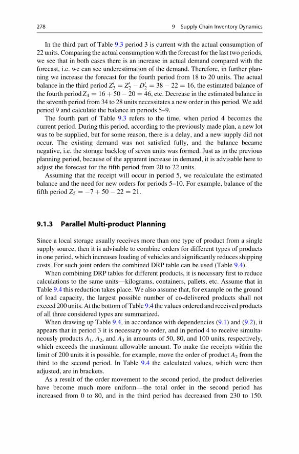
In the third part of Table 9.3 period 3 is current with the actual consumption of
22 units. Comparing the actual consumptionwith the forecast for the last two periods,
we see that in both cases there is an increase in actual demand compared with the
forecast, i.e. we can see underestimation of the demand. Therefore, in further plan-
ning we increase the forecast for the fourth period from 18 to 20 units. The actual
balance in the third period Z03 ¼ Z0
2 � D02 ¼ 38� 22 ¼ 16, the estimated balance of
the fourth period Z4 ¼ 16þ 50� 20 ¼ 46, etc. Decrease in the estimated balance in
the seventh period from 34 to 28 units necessitates a new order in this period.We add
period 9 and calculate the balance in periods 5–9.
The fourth part of Table 9.3 refers to the time, when period 4 becomes the
current period. During this period, according to the previously made plan, a new lot
was to be supplied, but for some reason, there is a delay, and a new supply did not
occur. The existing demand was not satisfied fully, and the balance became
negative, i.e. the storage backlog of seven units was formed. Just as in the previous
planning period, because of the apparent increase in demand, it is advisable here to
adjust the forecast for the fifth period from 20 to 22 units.
Assuming that the receipt will occur in period 5, we recalculate the estimated
balance and the need for new orders for periods 5–10. For example, balance of the
fifth period Z5 ¼ �7þ 50� 22 ¼ 21.
9.1.3 Parallel Multi-product Planning
Since a local storage usually receives more than one type of product from a single
supply source, then it is advisable to combine orders for different types of products
in one period, which increases loading of vehicles and significantly reduces shipping
costs. For such joint orders the combined DRP table can be used (Table 9.4).
When combining DRP tables for different products, it is necessary first to reduce
calculations to the same units—kilograms, containers, pallets, etc. Assume that in
Table 9.4 this reduction takes place. We also assume that, for example on the ground
of load capacity, the largest possible number of co-delivered products shall not
exceed 200 units. At the bottomof Table 9.4 the values ordered and received products
of all three considered types are summarized.
When drawing up Table 9.4, in accordance with dependencies (9.1) and (9.2), it
appears that in period 3 it is necessary to order, and in period 4 to receive simulta-
neously products A1, A2, and A3 in amounts of 50, 80, and 100 units, respectively,
which exceeds the maximum allowable amount. To make the receipts within the
limit of 200 units it is possible, for example, move the order of product A2 from the
third to the second period. In Table 9.4 the calculated values, which were then
adjusted, are in brackets.
As a result of the order movement to the second period, the product deliveries
have become much more uniform—the total order in the second period has
increased from 0 to 80, and in the third period has decreased from 230 to 150.
278 9 Supply Chain Inventory Dynamics
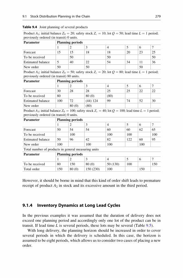
However, it should be borne in mind that this kind of order shift leads to premature
receipt of product A2 in stock and its excessive amount in the third period.
9.1.4 Inventory Dynamics at Long Lead Cycles
In the previous examples it was assumed that the duration of delivery does not
exceed one planning period and accordingly only one lot of the product can be in
transit. If lead time L is several periods, these lots may be several (Table 9.5).
With long delivery, the planning horizon should be increased in order to cover
several periods in which the delivery is scheduled. In this case, the horizon is
assumed to be eight periods, which allows us to consider two cases of placing a new
order.
Table 9.4 Joint planning of several products
Product A1; initial balance Z0 ¼ 20; safety stock Zc ¼ 10; lot Q ¼ 50; lead time L ¼ 1 period;
previously ordered (in transit) 0 units.
Parameter Planning periods
1 2 3 4 5 6 7
Forecast 15 15 18 18 20 23 25
To be received 50 50 50
Estimated balance 5 40 22 54 34 11 36
New order 50 50 50
Product A2; initial balance Z0 ¼ 50; safety stock Zc ¼ 20; lot Q ¼ 80; lead time L ¼ 1 period;
previously ordered (in transit) 80 units.
Parameter Planning periods
1 2 3 4 5 6 7
Forecast 30 28 28 25 25 22 22
To be received 80 80 (0) (80)
Estimated balance 100 72 (44) 124 99 74 52 30
New order 80 (0) (80)
Product A3; initial balance Z0 ¼ 100; safety stock Zc ¼ 40; lot Q ¼ 100; lead time L ¼ 1 period;
previously ordered (in transit) 0 units.
Parameter Planning periods
1 2 3 4 5 6 7
Forecast 50 54 54 60 60 62 65
To be received 100 100 100 100
Estimated balance 50 96 42 82 122 60 95
New order 100 100 100 100
Total number of products in general measuring units
Parameter Planning periods
1 2 3 4 5 6 7
To be received 80 150 80 (0) 50 (130) 100 150
Total order 150 80 (0) 150 (230) 100 150
9.1 Stock Distribution Planning in the Chain 279
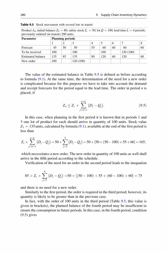
The value of the estimated balance in Table 9.5 is defined as before according
to formula (9.1). At the same time, the determination of the need for a new order
is complicated because for this purpose we have to take into account the demand
and receipt forecasts for the period equal to the lead time. The order in period n is
placed, if
Zn � Zc þXnþL
j¼nþ1
Dj � Qj
� : ð9:5Þ
In this case, when planning in the first period it is known that in periods 1 and
3 one lot of product for each should arrive in quantity of 100 units. Stock value
Z1 ¼ 135 units, calculated by formula (9.1), available at the end of the first period is
less than
ZcþXnþL
j¼nþ1
Dj�Qj
� ¼50þX5j¼2
Dj�Qj
� ¼50þ 50þ 50�100ð Þþ55þ66½ �¼165;
which necessitates a new order. The new order in quantity of 100 units as well shall
arrive in the fifth period according to the schedule.
Verification of the need for an order in the second period leads to the inequation
85 > Zc þX6j¼3
Dj � Qj
� ¼50þ 50� 100ð Þ þ 55þ 60� 100ð Þ þ 60½ � ¼ 75
and there is no need for a new order.
Similarly to the first period, the order is required in the third period; however, its
quantity is likely to be greater than in the previous case.
In fact, with the order of 100 units in the third period (Table 9.5, this value is
given in brackets), the planned balance of the fourth period may be insufficient to
ensure the consumption in future periods. In this case, in the fourth period, condition
(9.5) gives
Table 9.5 Stock movement with several lots in transit
Product A4; initial balance Z0 ¼ 80; safety stock Zc ¼ 50; lot Q ¼ 100; lead time L ¼ 4 periods;
previously ordered (in transit) 200 units.
Parameter Planning periods
1 2 3 4 5 6 7 8
Forecast 45 50 50 55 60 60 60 60
To be received 100 100 100 120 (100)
Estimated balance 135 85 135 80 120 60 120 60
New order 100 120 (100)
280 9 Supply Chain Inventory Dynamics
80 < Zc þX8j¼5
Dj � Qj
� ¼50þ 60� 100ð Þ þ 60þ 60� 100ð Þ þ 60½ � ¼ 90;
which causes the need for a new order. If the quantity of the ordered lot is not
determined by any additional terms and conditions, in this case it is advisable to
increase the size of the lot, and so satisfy a tendency to increase in demand. Suppose,
for example, the size of the lot ordered in the third period is 120 units. In this case,
the need for additional orders in the fourth period will disappear.
The estimated balance in this case can be set for all periods up to the horizon
under consideration; at the same time to determine the need for a new order in the
fifth period, the forecast horizon of eight periods is insufficient and therefore this
need has to be defined in the next planning cycle.
9.2 Supply Chain Fluctuations
Changes in demand, as discussed above in Sect. 6.1, are defined by the trend, on
which random fluctuations are superimposed. Besides, the demand can make
regular oscillatory motion about the main direction (trend) due to seasonal changes
in demand, promotions, etc. The direction of the trend can also vary due to changes
in fashion, competition, general economic situation, etc.
Changes in the demand at the point of final sales of the product cause changes in
orders for the product itself, and then to its components, materials, and subsequently
to the equipment for manufacturing the product and all its components. Passing
through the supply chain, the changes in the order quantity gradually deviate from
the initial changes in demand, and such deviations are often growing in nature.
The reasons for this phenomenon are rooted in the use of forecasting for order
placement. As the forecasts are based on statistical data, they always contain errors,
for which the possibility of correcting is provided by safety stocks in orders. The
accumulation of errors by moving up the supply chain leads to an increase in safety
stocks. When the trend direction in demand changes, the wave of changes in safety
stocks propagate throughout the chain. The amplitude of the wave increases with
distance from the end user. This phenomenon is called Forrester effect or bullwhip
effect. The latter name is due to the analogy with the shape of oscillations with
increasing amplitude, which a shepherd’s whip takes.
9.2.1 Bullwhip Effect
To demonstrate the mechanism of the bullwhip effect, we shall consider the process
of change in sales and orders for the chain consisting of three echelons (Table 9.6).
In Table 9.6, 13 periods of supply chain operation are considered in form of a
relevant DRP table, and it is believed that up to and including the first period sales
9.2 Supply Chain Fluctuations 281
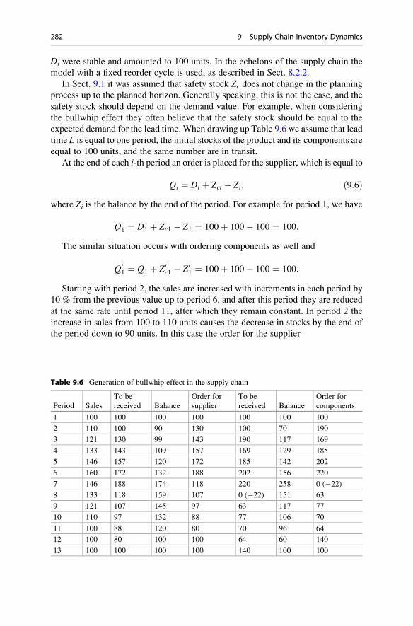
Di were stable and amounted to 100 units. In the echelons of the supply chain the
model with a fixed reorder cycle is used, as described in Sect. 8.2.2.
In Sect. 9.1 it was assumed that safety stock Zc does not change in the planning
process up to the planned horizon. Generally speaking, this is not the case, and the
safety stock should depend on the demand value. For example, when considering
the bullwhip effect they often believe that the safety stock should be equal to the
expected demand for the lead time. When drawing up Table 9.6 we assume that lead
time L is equal to one period, the initial stocks of the product and its components are
equal to 100 units, and the same number are in transit.
At the end of each i-th period an order is placed for the supplier, which is equal to
Qi ¼ Di þ Zci � Zi; ð9:6Þwhere Zi is the balance by the end of the period. For example for period 1, we have
Q1 ¼ D1 þ Zc1 � Z1 ¼ 100þ 100� 100 ¼ 100:
The similar situation occurs with ordering components as well and
Q01 ¼ Q1 þ Z0
c1 � Z01 ¼ 100þ 100� 100 ¼ 100:
Starting with period 2, the sales are increased with increments in each period by
10 % from the previous value up to period 6, and after this period they are reduced
at the same rate until period 11, after which they remain constant. In period 2 the
increase in sales from 100 to 110 units causes the decrease in stocks by the end of
the period down to 90 units. In this case the order for the supplier
Table 9.6 Generation of bullwhip effect in the supply chain
Period Sales
To be
received Balance
Order for
supplier
To be
received Balance
Order for
components
1 100 100 100 100 100 100 100
2 110 100 90 130 100 70 190
3 121 130 99 143 190 117 169
4 133 143 109 157 169 129 185
5 146 157 120 172 185 142 202
6 160 172 132 188 202 156 220
7 146 188 174 118 220 258 0 (�22)
8 133 118 159 107 0 (�22) 151 63
9 121 107 145 97 63 117 77
10 110 97 132 88 77 106 70
11 100 88 120 80 70 96 64
12 100 80 100 100 64 60 140
13 100 100 100 100 140 100 100
282 9 Supply Chain Inventory Dynamics

Q2 ¼ D2 þ Zc2 � Z2 ¼ 110þ 110� 90 ¼ 130;
and for components order we will obtain
Q02 ¼ Q2 þ Z0
c2 � Z02 ¼ 130þ 130� 70 ¼ 190:
Determining the quantities of orders in the same way up to period 13, we obtain
the values given in Table 9.6. Exact calculations by formula (9.6) for period 7 lead
to a negative amount of �22 in the order for components. In view of impossibility
of negative order, in Table 9.6 this order is considered to be zero.
The graphs in Fig. 9.1 indicate that in each successive echelon in the supply
chain the amplitude of fluctuations increases. Besides, the graphs show that there
are oscillations with increasing amplitude in the chain during orders transfer up the
chain. As a result, even after sales return to its original value, in the chain there are
still damped oscillations, duration of which depends on the chain echelon distance
from its beginning.
We assume that the demand changes occur in the echelon located at 0. We will
define the notion of fluctuations transfer factor from demand fluctuations to the first
echelon (level) of the supply chain
k01 ¼ ΔQ
Δt=ΔD
Δt; ð9:7Þ
where ΔQ is the increment of the quantity of the order for the supplier on interval
Δt and ΔD is the increment of demand on this interval. This factor indicated the
ratio of the slope angles of the order curve in echelon 1 to the sales curve for each
interval in Fig. 9.1. Similarly, the fluctuations transfer factor from the first echelon
to the second one is equal to
0
50
100
150
200
250
0 1 2 3 4 5 6 7 8 9 10 11 12 13 14
Sal
es a
nd o
rder
s
Periods
Orders in echelon 2
Sales
Orders in echelon 1
Fig. 9.1 Graphs of sales and orders in the chain echelons
9.2 Supply Chain Fluctuations 283
k12 ¼ ΔQ0
Δt=ΔQ
Δt: ð9:8Þ
The analysis of the graphs in Fig. 9.1 shows that the value of fluctuations transfer
factor in echelon 1 becomes large at the points of sudden changes of sales trend
and the factor in echelon 2—at break points on order curve in echelon 1. Thus, the
transfer factor is a function of changing in trend direction. If graphs in Fig. 9.1 were
smooth, it could be assumed that the transfer factor depends on the second deriva-
tive of the fluctuations curve in the previous echelon. However, the curves in
Fig. 9.1 are not differentiable, and therefore the fluctuations transfer factor k01(n)in period n depends on the difference
ΔDn
Δt� ΔDn�1
Δt; ð9:9Þ
and accordingly factor k12(n) depends on the difference
ΔQn
Δt� ΔQn�1
Δt: ð9:10Þ
Fluctuations of the discussed type can occur not only in the cooperation of several
enterprises, but also among departments of one enterprise engaged in sequential
processing and assembly of products (Sachko 2008).
9.2.2 Bullwhip Effect Factors
A detailed analysis of the factors contributing to the occurrence and scope of the
bullwhip effect is shown in the papers of Lee et al. (1997a, b). The article (Lee
et al. 1997a) lists the main causes of the bullwhip effect:
• Regular updating of the forecasted demand values;
• Demand aggregation for several periods into one lot;
• Fluctuations in the price of the product;
• Restriction of sales and fears of shortages.
Of all these factors, according to the authors (Lee et al. 1997a) the need for
a regular accounting of changes in demand is the most important. Indeed, with
demand changes it is necessary to replenish the changed current stock and to provide
necessary quantity of safety stock. As a result, as shown above in Sect. 9.2.1, in the
supply chain there is the oscillation process, which increases as the distance from the
supply echelon of the end consumer.
In the paper (Lee et al. 1997b), this process is studied for the case of so-called
autoregressive demand of the first order. In auto-regression, each value of the time
series is a linear function of the previous one or several previous values of this series.
In the first-order auto-regression only the previous value is used, in the second
284 9 Supply Chain Inventory Dynamics
order auto-regression—two, etc. Thus, the demand in period n is described by the
dependence
Dn ¼ aþ ρDn�1 þ ε; ð9:11Þwhere a is a certain constant, ε is the random deviation of demand, and factor ρ is
within—1 � ρ � 1. For this demand the optimal size of a lot ordered at the end of
observation period n is defined by the dependence
Qn ¼ρ 1� ρLþ1ð Þ
1� ρDn � Dn�1ð Þ þ Dn; ð9:12Þ
where L is the lead time in period of observation.
The most interesting case of this dependence is when ρ ! 1. Expanding the
resulting uncertainty by the L’Hospital’s rule, with ρ ¼ 1 we have
Qn ¼ Lþ 1ð Þ Dn � Dn�1ð Þ þ Dn ¼ Dn þ Lþ 1ð ÞΔDn: ð9:13ÞFrom Eq. (9.13), it follows that the quantity of the ordered lot directly depends on
the lead time, which naturally leads to an increase in the amplitude of fluctuations in
the supply chain with the increase of lead time.
By starting consideration of the influence of demand aggregation, we note that
the order for a new receipt is created, for the most part, not after each consumption,
but only after its reduction to a certain value determined by some stock management
model (Sect. 8.2). Here all the demand for stock replenishment cycle is aggregated
into a single lot that can significantly reduce transportation costs. Figure 9.2 shows
the graphs of sales and orders in the first echelon of the supply chain for the data in
Table 9.6 with the order lot of 300 units. The orders schedule in echelon 2 in this
case coincides with the graph for echelon 1.
From Fig. 9.2, it follows that the application of the model with fixed order
quantity leads to significant fluctuations in demand at all levels of the supply chain.
At the same time, the change of the parameters of such fluctuations due to changes
in demand is small.
Temporary, for instance during the holidays, discount prices of the product may
cause a significant increase in demand and therefore sales revenue. However, such
measures often entail a drop in demand in subsequent periods, resulting in the
observed significant fluctuations in orders, destabilizing the production process.
Therefore, such pricing policy is justified mostly only when there are excessively
large stocks complicating their storage.
If demand for the product significantly exceeds the capacity of its production,
restrictions are often imposed on the product deliveries to consumers. Usually the
manufacturer distributes such products among consumers proportionally according
to the orders placed. Naturally, the consumers knowing the possible limitation
exaggerate their needs. This leads to the fact that, in reality, when the production
9.2 Supply Chain Fluctuations 285
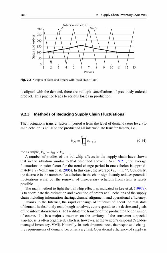
is aligned with the demand, there are multiple cancellations of previously ordered
product. This practice leads to serious losses in production.
9.2.3 Methods of Reducing Supply Chain Fluctuations
The fluctuations transfer factor in period n from the level of demand (zero level) to
m-th echelon is equal to the product of all intermediate transfer factors, i.e.
k0m ¼Ym�1
i¼0
ki, iþ1; ð9:14Þ
for example, k02 ¼ k01 � k12:A number of studies of the bullwhip effects in the supply chain have shown
that in the situation similar to that described above in Sect. 9.2.1, the average
fluctuations transfer factor for the trend change period in one echelon is approxi-
mately 1.7 (Vollmann et al. 2005). In this case, the average k0m ¼ 1:7m. Obviously,the decrease in the number ofm echelons in the chain significantly reduces potential
fluctuations scale, but the removal of unnecessary echelons from chain is rarely
possible.
The main method to fight the bullwhip effect, as indicated in Lee et al. (1997a),
is to coordinate the estimation and execution of orders at all echelons of the supply
chain including information sharing, channel alignment, and operational efficiency.
Thanks to the Internet, the rapid exchange of information about the real state
of demand is absolutely real, though not always corresponds to the desires and goals
of the information sources. To facilitate the transfer of the product to the consumer,
of course, if it is a major consumer, on the territory of the consumer a special
warehouse is often organized, which is, however, at the vendor’s disposal (Vendor-
managed Inventory, VMI). Naturally, in such circumstances, the response to chang-
ing requirements of demand becomes very fast. Operational efficiency of supply is
0
50
100
150
200
250
300
1 2 3 4 5 6 7 8 9 10 11 12 13
Sal
es a
nd o
rder
s
Periods
SalesOrders in echelon 1
Fig. 9.2 Graphs of sales and orders with fixed size of lots
286 9 Supply Chain Inventory Dynamics
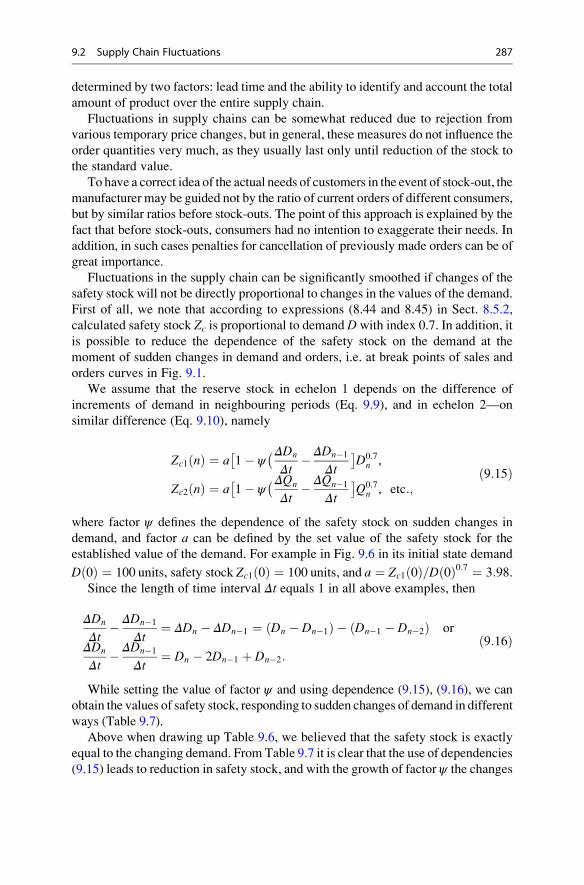
determined by two factors: lead time and the ability to identify and account the total
amount of product over the entire supply chain.
Fluctuations in supply chains can be somewhat reduced due to rejection from
various temporary price changes, but in general, these measures do not influence the
order quantities very much, as they usually last only until reduction of the stock to
the standard value.
To have a correct idea of the actual needs of customers in the event of stock-out, the
manufacturer may be guided not by the ratio of current orders of different consumers,
but by similar ratios before stock-outs. The point of this approach is explained by the
fact that before stock-outs, consumers had no intention to exaggerate their needs. In
addition, in such cases penalties for cancellation of previously made orders can be of
great importance.
Fluctuations in the supply chain can be significantly smoothed if changes of the
safety stock will not be directly proportional to changes in the values of the demand.
First of all, we note that according to expressions (8.44 and 8.45) in Sect. 8.5.2,
calculated safety stock Zc is proportional to demand Dwith index 0.7. In addition, it
is possible to reduce the dependence of the safety stock on the demand at the
moment of sudden changes in demand and orders, i.e. at break points of sales and
orders curves in Fig. 9.1.
We assume that the reserve stock in echelon 1 depends on the difference of
increments of demand in neighbouring periods (Eq. 9.9), and in echelon 2—on
similar difference (Eq. 9.10), namely
Zc1 nð Þ ¼ a�1� ψ
�ΔDn
Δt� ΔDn�1
Δt
D0:7
n ,
Zc2 nð Þ ¼ a�1� ψ
�ΔQn
Δt� ΔQn�1
Δt
Q0:7
n , etc:;ð9:15Þ
where factor ψ defines the dependence of the safety stock on sudden changes in
demand, and factor a can be defined by the set value of the safety stock for the
established value of the demand. For example in Fig. 9.6 in its initial state demand
D 0ð Þ ¼ 100 units, safety stock Zc1 0ð Þ ¼ 100 units, and a ¼ Zc1 0ð Þ=D 0ð Þ0:7 ¼ 3:98.Since the length of time interval Δt equals 1 in all above examples, then
ΔDn
Δt� ΔDn�1
Δt¼ ΔDn � ΔDn�1 ¼ Dn � Dn�1ð Þ � Dn�1 � Dn�2ð Þ or
ΔDn
Δt� ΔDn�1
Δt¼ Dn � 2Dn�1 þ Dn�2:
ð9:16Þ
While setting the value of factor ψ and using dependence (9.15), (9.16), we can
obtain the values of safety stock, responding to sudden changes of demand in different
ways (Table 9.7).
Above when drawing up Table 9.6, we believed that the safety stock is exactly
equal to the changing demand. From Table 9.7 it is clear that the use of dependencies
(9.15) leads to reduction in safety stock, and with the growth of factor ψ the changes
9.2 Supply Chain Fluctuations 287

Table
9.7
Changes
insafety
stock
dependingonthedem
and
Param
eters
Periods
01
23
45
67
89
10
11
Dem
and
100
100
110
121
133
146
160
146
133
121
110
100
Stock
atψ¼
0100
100
107
115
122
130
139
130
122
114
107
100
Stock
atψ¼
0:002
100
100
105
114
121
130
138
137
122
114
107
100
Stock
atψ¼
0:003
100
100
104
114
122
130
138
141
121
113
106
100
288 9 Supply Chain Inventory Dynamics
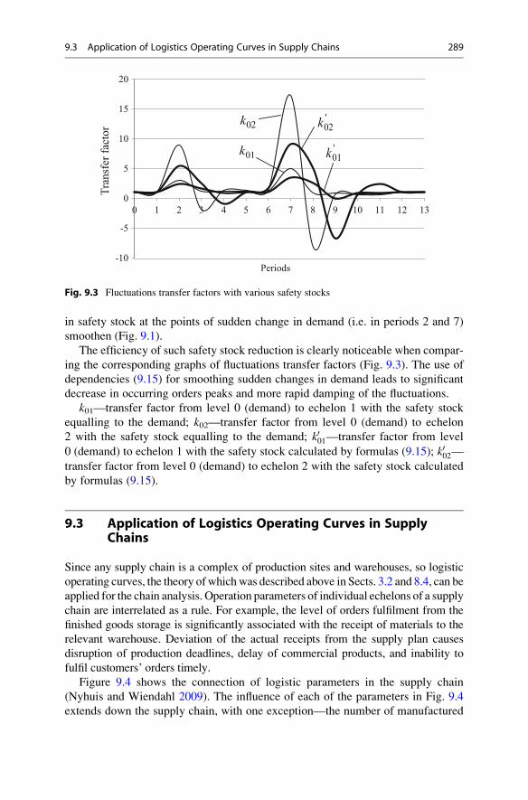
in safety stock at the points of sudden change in demand (i.e. in periods 2 and 7)
smoothen (Fig. 9.1).
The efficiency of such safety stock reduction is clearly noticeable when compar-
ing the corresponding graphs of fluctuations transfer factors (Fig. 9.3). The use of
dependencies (9.15) for smoothing sudden changes in demand leads to significant
decrease in occurring orders peaks and more rapid damping of the fluctuations.
k01—transfer factor from level 0 (demand) to echelon 1 with the safety stock
equalling to the demand; k02—transfer factor from level 0 (demand) to echelon
2 with the safety stock equalling to the demand; k001—transfer factor from level
0 (demand) to echelon 1 with the safety stock calculated by formulas (9.15); k002—transfer factor from level 0 (demand) to echelon 2 with the safety stock calculated
by formulas (9.15).
9.3 Application of Logistics Operating Curves in SupplyChains
Since any supply chain is a complex of production sites and warehouses, so logistic
operating curves, the theory ofwhichwas described above in Sects. 3.2 and 8.4, can be
applied for the chain analysis. Operation parameters of individual echelons of a supply
chain are interrelated as a rule. For example, the level of orders fulfilment from the
finished goods storage is significantly associated with the receipt of materials to the
relevant warehouse. Deviation of the actual receipts from the supply plan causes
disruption of production deadlines, delay of commercial products, and inability to
fulfil customers’ orders timely.
Figure 9.4 shows the connection of logistic parameters in the supply chain
(Nyhuis and Wiendahl 2009). The influence of each of the parameters in Fig. 9.4
extends down the supply chain, with one exception—the number of manufactured
-10
-5
0
5
10
15
20
0 1 2 3 4 5 6 7 8 9 10 11 12 13
Tra
nsf
er f
acto
r
Periods
01k
02k '02k
'01k
Fig. 9.3 Fluctuations transfer factors with various safety stocks
9.3 Application of Logistics Operating Curves in Supply Chains 289
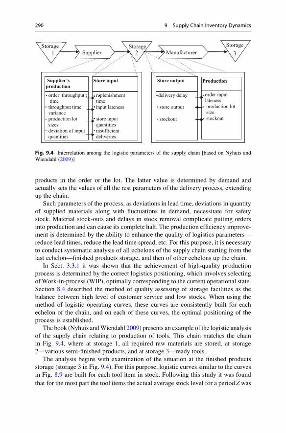
products in the order or the lot. The latter value is determined by demand and
actually sets the values of all the rest parameters of the delivery process, extending
up the chain.
Such parameters of the process, as deviations in lead time, deviations in quantity
of supplied materials along with fluctuations in demand, necessitate for safety
stock. Material stock-outs and delays in stock removal complicate putting orders
into production and can cause its complete halt. The production efficiency improve-
ment is determined by the ability to enhance the quality of logistics parameters—
reduce lead times, reduce the lead time spread, etc. For this purpose, it is necessary
to conduct systematic analysis of all echelons of the supply chain starting from the
last echelon—finished products storage, and then of other echelons up the chain.
In Sect. 3.3.1 it was shown that the achievement of high-quality production
process is determined by the correct logistics positioning, which involves selecting
of Work-in-process (WIP), optimally corresponding to the current operational state.
Section 8.4 described the method of quality assessing of storage facilities as the
balance between high level of customer service and low stocks. When using the
method of logistic operating curves, these curves are consistently built for each
echelon of the chain, and on each of these curves, the optimal positioning of the
process is established.
The book (Nyhuis andWiendahl 2009) presents an example of the logistic analysis
of the supply chain relating to production of tools. This chain matches the chain
in Fig. 9.4, where at storage 1, all required raw materials are stored, at storage
2—various semi-finished products, and at storage 3—ready tools.
The analysis begins with examination of the situation at the finished products
storage (storage 3 in Fig. 9.4). For this purpose, logistic curves similar to the curves
in Fig. 8.9 are built for each tool item in stock. Following this study it was found
that for the most part the tool items the actual average stock level for a period Zwas
Supplier ManufacturerStorage
Supplier’s production
Store input Store output Production
order throughput ;time
throughput time varianceproduction lot sizes deviation of inputquantities
replenishment timeinput lateness
store input quantitiesinsufficient deliveries
delivery delay
store output
stockout
order input latenessproduction lot size
stockout
Storage Storage
1 2 3
Fig. 9.4 Interrelation among the logistic parameters of the supply chain [based on Nyhuis and
Wiendahl (2009)]
290 9 Supply Chain Inventory Dynamics
greater than stock levelZ1 providing zero delay of deliverywith regard to the required
safety stock, i.e. clearly excessive stocks of finished products were observed. For
some items, on the contrary, the stock was insufficient and did not provide tools
supply with the required level of customer service.
The results of this operation led to the fact that the initial number of tools of
3.5 million pcs. valued at 5.9 million euros has been reduced to the quantity of 2.2
million pcs. valued at 3.3 million euros. Thus, only due to the performance analysis
of the finished products storage it has appeared to be possible to reduce the stock by
approx. 40 %.
Logistic analysis has also helped to establish the structure of stocks typical for
the production under study. It turned out that the variable component of stocks
caused by the receipt and withdrawal of the product lots amounts to only 43.1 % of
the stock, and the bigger part (56.9 %) is the safety stock. All safety stock in the
study was divided into three parts: the safety stock for fluctuations in demand,
which is 36.7 % of the total stock; stock for delays in orders delivery amounting to
19.6 %; and the stock insuring an insufficient number of goods in the supply is only
0.7 % of the total value of the stock. Determining the stock structure helped to define
the measures to further reduce stocks—marketing efforts to stabilize demand,
reducing the production lot size for individual items, delivery regulation, etc.
At the next stage the tool production as such was studied. For production
bottlenecks logistics operating curves similar to the curves in Figs. 3.7 and 3.10
were built and the solutions were developed to improve the performance of
bottlenecks using the methods described in Sect. 3.3.2. Following these activities
the average duration of production cycleF could be reduced from 32.5 working days
to 15.5 working days. This result was achieved due to reducing average workloadWby about 50 %.
Analysis of the performance of themanufacturer’s storage for incomingmaterials
and semi-finished products (storage 2 in Fig. 9.4) showed that the supplying enter-
prise fulfils the orders of the manufacturing enterprise with a standard deviation of
lead time of 6.4 working days. As the planned deviation of the finished product
output is only 1.2 working days, the lead time spread of 6.4 days makes the
manufacturer keep high safety stocks.
The second reason for large stocks at the incoming materials storage is that the
size of the delivery lots source materials and semi-finished products are usually
much higher than the size of the finished product lots. The use of ABC classification
allowed grouping the various items of materials into groups A, B, and C and
matching each group with the required service level. For example, for group A,
as known, being 20 % of all the supply items, level of service SL is required to
approach 100 %. Accordingly, by setting a lower level of service for groups B
and C, the required amount of safety stock was reduced.
At the last stage of the described study, the production activity of the suppliers
was examined. For this purpose, the above-described technique of identification of
bottlenecks and logistics positioning was applied.
9.3 Application of Logistics Operating Curves in Supply Chains 291
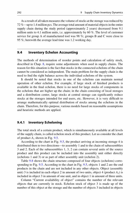
As a result of all takenmeasures the volume of stocks at the storage was reduced by
72%—up to 1.4million pcs. The average total amount ofmaterial objects in the entire
supply chain during the study period (approximately 2 years) decreased from 9.1
million units to 4.1 million units, i.e. approximately by 60 %. The level of customer
service for group A of manufactured tool was 98 %; groups B and C were close to
95 %; herewith the average lead time was 1.2 working day.
9.4 Inventory Echelon Accounting
The methods of determination of reorder points and calculation of safety stock,
described in Chap. 8, require some adjustments when used in supply chains. The
reason for this situation is the fact that stocks in the connected echelons of the chain
cannot be considered as independent. The main problem for the supply chain is the
need to find the right balance across the individual echelons of the system.
It should be noted that stocks in one of the echelons can maintain normal
operation of other echelon. For example, if large stock of finished products is
available in the final echelon, there is no need for large stocks of components in
the echelons that are higher up the chain; in the chain consisting of local storages
and a distribution center, large stocks at central storage can significantly reduce
stocks at the storages intended for end users, etc. However, it is very difficult to
arrange mathematically optimal distribution of stocks among the echelons in the
chain. Therefore, for this purpose, various models based on reasonable assumptions
and heuristic methods are applied.
9.4.1 Inventory Echeloning
The total stock of a certain product, which is simultaneously available at all levels
of the supply chain, is called echelon stock of this product. Let us consider the chart
of product A1 shown in Fig. 9.5.
According to the chart in Fig. 9.5, the product arriving at incoming storage 4 is
distributed then to two directions—to assembly 1 and to the chain of subassemblies
3 and 2. Each of the subassemblies 1, 3, 2 can contain several units of the source
product and this product can be included into the assembly unit either directly
(echelons 1 and 3) or as part of other assembly unit (echelon 2).
Table 9.8 shows the chain structure composed of four objects (echelons) corre-
sponding to Fig. 9.5. According to the chart in Fig. 9.5, objects 1 and 2 are the end
products in the chain and are not included in any other objects. Object (assembly
unit) 3 is included in each object 2 in amount of two units, object 4 (product A1) is
included in object 3 in amount of one unit, and in object 1 in amount of three units.
Column “Current availability of object” contains the number of the relevant
objects that are currently in stock. Echelon stock of object 3 is made up of the
number of this object at the storage and the number of objects 3 included in objects
292 9 Supply Chain Inventory Dynamics
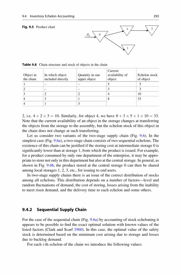
2, i.e. 4þ 2� 3 ¼ 10. Similarly, for object 4, we have 8þ 3� 5þ 1� 10 ¼ 33.
Note that the current availability of an object in the storage changes at transferring
the objects from the storage to the assembly, but the echelon stock of this object in
the chain does not change at such transferring.
Let us consider two variants of the two-stage supply chain (Fig. 9.6). In the
simplest case (Fig. 9.6a), a two-stage chain consists of two sequential echelons. The
existence of this chain can be justified if the storing cost at intermediate storage 0 is
significantly lower than at storage 1, from which the product is issued. For example,
for a product consumed by only one department of the enterprise, it may be appro-
priate to store not only in this department but also at the central storage. In general, as
shown in Fig. 9.6b, the product stored at the central storage 0 can then be shared
among local storages 1, 2, 3, etc., for issuing to end users.
In two-stage supply chains there is an issue of the correct distribution of stocks
among all echelons. This distribution depends on a number of factors—level and
random fluctuations of demand, the cost of storing, losses arising from the inability
to meet risen demand, and the delivery time to each echelon and some others.
9.4.2 Sequential Supply Chain
For the case of the sequential chain (Fig. 9.6a) by accounting of stock echeloning it
appears to be possible to find the exact optimal solution with known values of the
listed factors (Clark and Scarf 1960). In this case, the optimal value of the safety
stock is determined based on the minimum cost arising due to storage and losses
due to backlog demand.
For each i-th echelon of the chain we introduce the following values:
4
3 2
1
1A
Fig. 9.5 Product chart
Table 9.8 Chain structure and stock of objects in the chain
Object in
the chain
In which object
included directly
Quantity in one
upper object
Current
availability of
object
Echelon stock
of object
1 – – 5 5
2 – – 3 3
3 2 2 4 10
4 3 1 8 33
4 1 3
9.4 Inventory Echelon Accounting 293
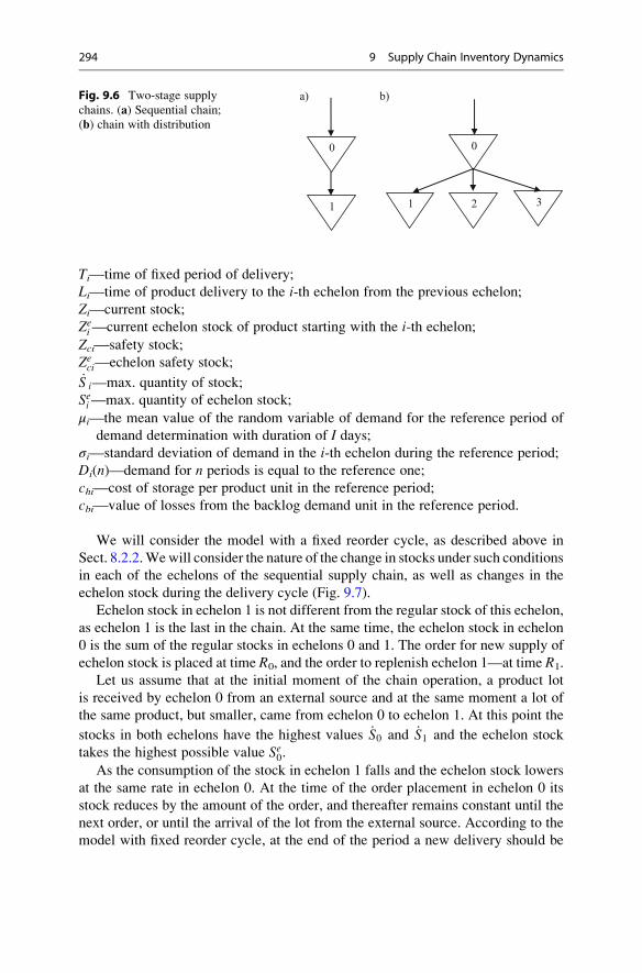
Ti—time of fixed period of delivery;
Li—time of product delivery to the i-th echelon from the previous echelon;
Zi—current stock;
Zei—current echelon stock of product starting with the i-th echelon;
Zci—safety stock;
Zeci—echelon safety stock;_S i—max. quantity of stock;
Sei—max. quantity of echelon stock;
μi—the mean value of the random variable of demand for the reference period of
demand determination with duration of I days;σi—standard deviation of demand in the i-th echelon during the reference period;
Di(n)—demand for n periods is equal to the reference one;
chi—cost of storage per product unit in the reference period;
cbi—value of losses from the backlog demand unit in the reference period.
We will consider the model with a fixed reorder cycle, as described above in
Sect. 8.2.2.Wewill consider the nature of the change in stocks under such conditions
in each of the echelons of the sequential supply chain, as well as changes in the
echelon stock during the delivery cycle (Fig. 9.7).
Echelon stock in echelon 1 is not different from the regular stock of this echelon,
as echelon 1 is the last in the chain. At the same time, the echelon stock in echelon
0 is the sum of the regular stocks in echelons 0 and 1. The order for new supply of
echelon stock is placed at time R0, and the order to replenish echelon 1—at time R1.
Let us assume that at the initial moment of the chain operation, a product lot
is received by echelon 0 from an external source and at the same moment a lot of
the same product, but smaller, came from echelon 0 to echelon 1. At this point the
stocks in both echelons have the highest values _S0 and _S1 and the echelon stock
takes the highest possible value Se0.As the consumption of the stock in echelon 1 falls and the echelon stock lowers
at the same rate in echelon 0. At the time of the order placement in echelon 0 its
stock reduces by the amount of the order, and thereafter remains constant until the
next order, or until the arrival of the lot from the external source. According to the
model with fixed reorder cycle, at the end of the period a new delivery should be
0
1
0
1 2 3
a) b)Fig. 9.6 Two-stage supply
chains. (a) Sequential chain;(b) chain with distribution
294 9 Supply Chain Inventory Dynamics
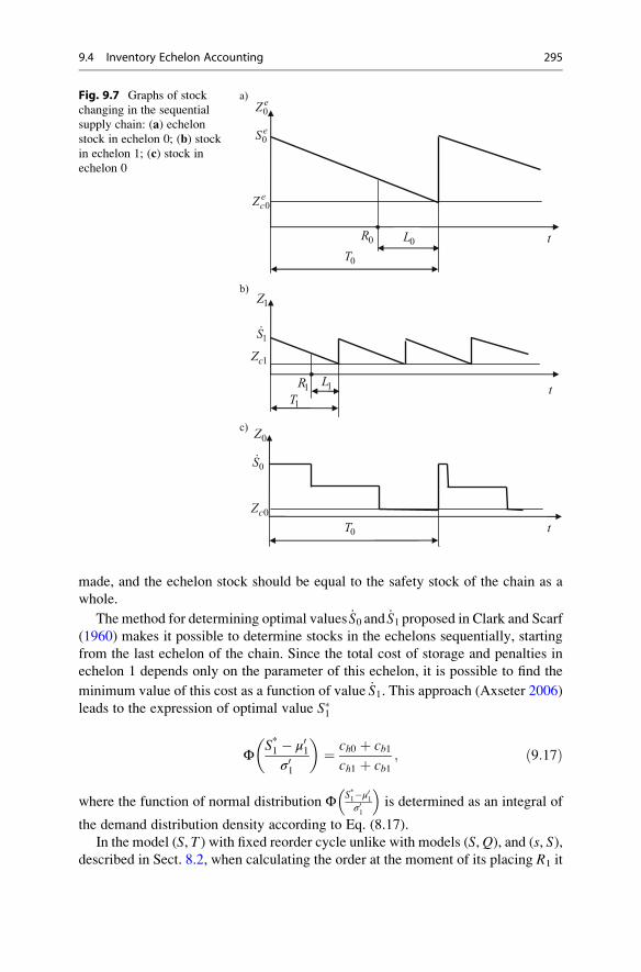
made, and the echelon stock should be equal to the safety stock of the chain as a
whole.
The method for determining optimal values _S0 and _S1 proposed in Clark and Scarf(1960) makes it possible to determine stocks in the echelons sequentially, starting
from the last echelon of the chain. Since the total cost of storage and penalties in
echelon 1 depends only on the parameter of this echelon, it is possible to find the
minimum value of this cost as a function of value _S1. This approach (Axseter 2006)leads to the expression of optimal value S1
ΦS*1 � μ01
σ01
� �¼ ch0 þ cb1
ch1 þ cb1; ð9:17Þ
where the function of normal distribution Φ S*1�μ01
σ01
� �is determined as an integral of
the demand distribution density according to Eq. (8.17).
In the model (S, T ) with fixed reorder cycle unlike with models (S, Q), and (s, S),described in Sect. 8.2, when calculating the order at the moment of its placing R1 it
0R
1R
0cZ
0Z
0S
0eZ
0ecZ
0eS
1L1T
1Z
1cZ1S
0L
0Tt
t
0T t
a)
b)
c)
.
.
Fig. 9.7 Graphs of stock
changing in the sequential
supply chain: (a) echelonstock in echelon 0; (b) stockin echelon 1; (c) stock in
echelon 0
9.4 Inventory Echelon Accounting 295
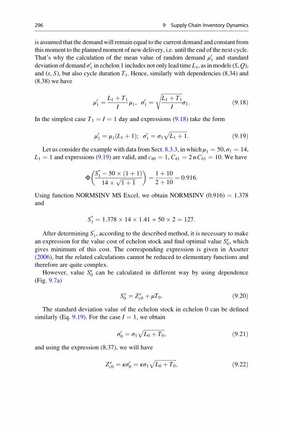
is assumed that the demandwill remain equal to the current demand and constant from
thismoment to the plannedmoment of new delivery, i.e. until the end of the next cycle.
That’s why the calculation of the mean value of random demand μ01 and standard
deviation of demand σ01 in echelon 1 includes not only lead time L1, as inmodels (S,Q),and (s, S), but also cycle duration T1. Hence, similarly with dependencies (8.34) and
(8.38) we have
μ01 ¼L1 þ T1
Iμ1, σ01 ¼
ffiffiffiffiffiffiffiffiffiffiffiffiffiffiffiffiL1 þ T1
I
rσ1: ð9:18Þ
In the simplest case T1 ¼ I ¼ 1 day and expressions (9.18) take the form
μ01 ¼ μ1 L1 þ 1ð Þ; σ01 ¼ σ1ffiffiffiffiffiffiffiffiffiffiffiffiffiL1 þ 1
p: ð9:19Þ
Let us consider the example with data from Sect. 8.3.3, in whichμ1 ¼ 50,σ1 ¼ 14,
L1 ¼ 1 and expressions (9.19) are valid, and ch0 ¼ 1, Ch1 ¼ 2иCb1 ¼ 10. We have
ΦS*1 � 50� 1þ 1ð Þ
14� ffiffiffiffiffiffiffiffiffiffiffi1þ 1
p� �
¼ 1þ 10
2þ 10¼ 0:916:
Using function NORMSINV MS Excel, we obtain NORMSINV (0.916) ¼ 1.378
and
S*1 ¼ 1:378� 14� 1:41þ 50� 2 ¼ 127:
After determining S1, according to the described method, it is necessary to make
an expression for the value cost of echelon stock and find optimal value Se0, whichgives minimum of this cost. The corresponding expression is given in Axseter
(2006), but the related calculations cannot be reduced to elementary functions and
therefore are quite complex.
However, value Se0 can be calculated in different way by using dependence
(Fig. 9.7a)
Se0 ¼ Z e
c0 þ μT0: ð9:20ÞThe standard deviation value of the echelon stock in echelon 0 can be defined
similarly (Eq. 9.19). For the case I ¼ 1, we obtain
σ00 ¼ σ1ffiffiffiffiffiffiffiffiffiffiffiffiffiffiffiffiL0 þ T0
p; ð9:21Þ
and using the expression (8.37), we will have
Z ec0 ¼ κσ00 ¼ κσ1
ffiffiffiffiffiffiffiffiffiffiffiffiffiffiffiffiL0 þ T0
p; ð9:22Þ
296 9 Supply Chain Inventory Dynamics
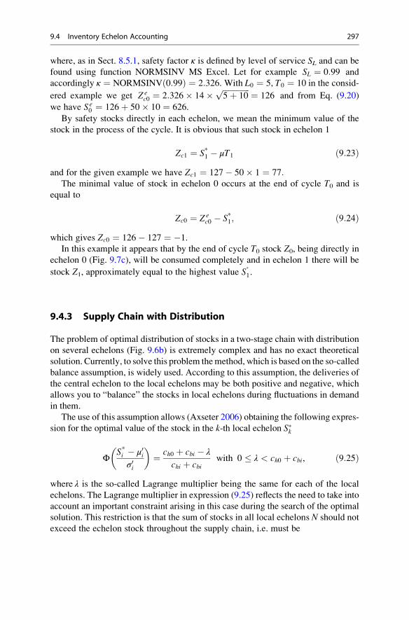
where, as in Sect. 8.5.1, safety factor κ is defined by level of service SL and can be
found using function NORMSINV MS Excel. Let for example SL ¼ 0:99 and
accordingly κ ¼ NORMSINV 0:99ð Þ ¼ 2:326. With L0 ¼ 5, T0 ¼ 10 in the consid-
ered example we get Z ec0 ¼ 2:326� 14� ffiffiffiffiffiffiffiffiffiffiffiffiffiffi
5þ 10p ¼ 126 and from Eq. (9.20)
we have Se0 ¼ 126þ 50� 10 ¼ 626.
By safety stocks directly in each echelon, we mean the minimum value of the
stock in the process of the cycle. It is obvious that such stock in echelon 1
Zc1 ¼ S*1 � μT1 ð9:23Þand for the given example we have Zc1 ¼ 127� 50� 1 ¼ 77:
The minimal value of stock in echelon 0 occurs at the end of cycle T0 and is
equal to
Zc0 ¼ Z ec0 � S*1; ð9:24Þ
which gives Zc0 ¼ 126� 127 ¼ �1.
In this example it appears that by the end of cycle T0 stock Z0, being directly in
echelon 0 (Fig. 9.7c), will be consumed completely and in echelon 1 there will be
stock Z1, approximately equal to the highest value S1.
9.4.3 Supply Chain with Distribution
The problem of optimal distribution of stocks in a two-stage chain with distribution
on several echelons (Fig. 9.6b) is extremely complex and has no exact theoretical
solution. Currently, to solve this problem themethod, which is based on the so-called
balance assumption, is widely used. According to this assumption, the deliveries of
the central echelon to the local echelons may be both positive and negative, which
allows you to “balance” the stocks in local echelons during fluctuations in demand
in them.
The use of this assumption allows (Axseter 2006) obtaining the following expres-
sion for the optimal value of the stock in the k-th local echelon Sk
ΦS*i � μ0i
σ0i
� �¼ ch0 þ cbi � λ
chi þ cbiwith 0 � λ < ch0 þ cbi, ð9:25Þ
where λ is the so-called Lagrange multiplier being the same for each of the local
echelons. The Lagrange multiplier in expression (9.25) reflects the need to take into
account an important constraint arising in this case during the search of the optimal
solution. This restriction is that the sum of stocks in all local echelons N should not
exceed the echelon stock throughout the supply chain, i.e. must be
9.4 Inventory Echelon Accounting 297
XNi¼1
S*i � Se0 : ð9:26Þ
In most of the numerous papers devoted to the study of this problem, attempts
are made to find the limits, within which the stocks at all echelons of the two-stage
chain can be present. Thus, in the same way as above in Sect. 9.4.2, they are based
on the minimum cost arising due to storage costs and losses due to backlog demand.
Since, however, the optimal distribution of the chain can be strongly affected by
various other factors such as transport costs, ability to transfer stocks from one
storage to another, etc., the practical application of the results of the above studies is
difficult.
In this situation, it seems appropriate to use expression (9.25) as the basis for
selection of the relations between stocks in echelons of the real-life chain. To do
this, by varying value λ, it is possible to determine the relation of the minimum
value of the stock in echelon 0 and echelon safety stock in this echelon and then
evaluate its validity on the basis of available experience.
The value of echelon safety stock with reference demand period I ¼ 1 for the
chain with distribution is equal to (Cao and Silver 2005)
Z ec0 ¼ κ
ffiffiffiffiffiffiffiffiffiffiffiffiffiffiffiffiffiffiffiffiffiffiffiffiffiffiffiffiffiffiffiffiL0 þ T0ð Þ
XNi¼1
σ2i
vuut : ð9:27Þ
As stock changes in local echelons are random, the minimum value of the stock
in echelon 0, similarly to Eq. (9.23), we have
Zc0 ¼ Z ec0 �
ffiffiffiffiffiffiffiffiffiffiffiffiffiffiffiffiffiffiffiXNi¼1
S*i� 2vuut : ð9:28Þ
Let us consider an example, in which a two-stage chain has a central echelon and
three local echelons (Fig. 9.6b) with initial data given in Table 9.9.
For the data in Table 9.9 according to Eq. (9.27) the value of the echelon safety
stock with safety factor k ¼ 2:326, providing level of service SL ¼ 0:99
Z ec0 ¼ 2:326�
ffiffiffiffiffiffiffiffiffiffiffiffiffiffiffiffiffiffiffiffiffiffiffiffiffiffiffiffiffiffiffiffiffiffiffiffiffiffiffiffiffiffiffiffiffiffiffiffiffiffiffiffiffi5þ 10ð Þ 142 þ 142 þ 202
� q¼ 254:
Table 9.10 presents the calculation results of optimal stocks in echelons 1, 2, and
3 and safety stock in echelon 0 for different values of λ within the range meeting the
condition (9.25), i.e. at λ < 11.
Value of the optimal stock in echelon 1 at λ ¼ 0, of course, coincides with the
value of the stock received in Sect. 9.4.2 above, since the corresponding original
data match. The values of safety stock in echelon 0 are calculated from expression
(9.28); coefficient of safety stock in echelon 0 is defined as the ratio of the safety
298 9 Supply Chain Inventory Dynamics
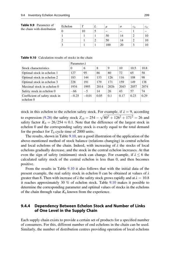
stock in this echelon to the echelon safety stock. For example, if λ ¼ 9, according
to expression (9.28) the safety stock Zc0 ¼ 254�ffiffiffiffiffiffiffiffiffiffiffiffiffiffiffiffiffiffiffiffiffiffiffiffiffiffiffiffiffiffiffiffiffiffiffiffiffi802 þ 1262 þ 1712
p¼ 26 and
safety factor K0 ¼ 26=254 � 0:1. Note that the difference of the largest stock in
echelon 0 and the corresponding safety stock is exactly equal to the total demand
for the product for T0 cycle time of 2000 units.
The results, shown in Table 9.10, are a good illustration of the application of the
above-mentioned method of stock balance (relations changing) in central echelon
and local echelons of the chain. Indeed, with increasing of λ the stocks of local
echelons gradually decrease, and the stock in the central echelon increases. At that
even the sign of safety (minimum) stock can change. For example, if λ � 6 the
calculated safety stock of the central echelon is less than 0, and then becomes
positive.
From the results in Table 9.10 it also follows that with the initial data of the
present example, the real safety stock in echelon 0 can be obtained at values of λgreater than 8. Then with increase of λ the safety stock grows rapidly and at λ ¼ 10:8it reaches approximately 30 % of echelon stock. Table 9.10 makes it possible to
determine the corresponding parameter and optimal values of stocks in the echelons
of the chain through value K0 known from the experience.
9.4.4 Dependency Between Echelon Stock and Number of Linksof One Level in the Supply Chain
Each supply chain exists to provide a certain set of products for a specified number
of consumers. For this, different number of end echelons in the chain can be used.
Similarly, the number of distribution centres providing operation of local echelons
Table 9.9 Parameter of
the chain with distributionEchelon T L μ σ ch cb
0 10 5 – – 1 –
1 1 1 50 14 2 10
2 1 2 50 14 2 10
3 1 1 100 20 3 10
Table 9.10 Calculation results of stocks in the chain
Stock characteristics
Parameter λ
0 6 8 9 10 10.5 10.8
Optimal stock in echelon 1 127 95 86 80 72 65 58
Optimal stock in echelon 2 183 144 133 126 116 108 98
Optimal stock in echelon 3 228 191 179 171 159 149 138
Maximal stock in echelon 0 1934 1995 2014 2026 2043 2057 2074
Safety stock in echelon 0 �66 �5 14 26 43 57 74
Coefficient of safety stock in
echelon 0
�0.25 �0.01 0.05 0.1 0.17 0.23 0.29
9.4 Inventory Echelon Accounting 299
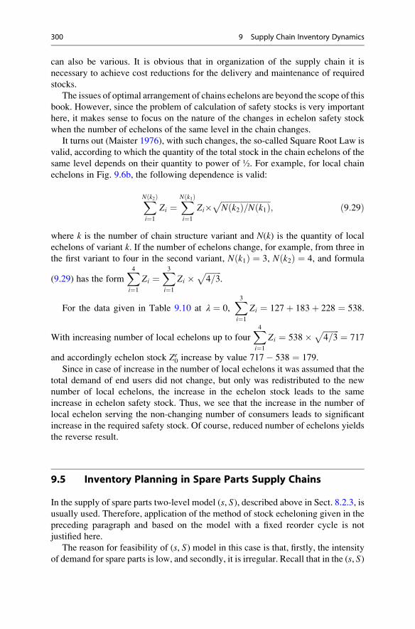
can also be various. It is obvious that in organization of the supply chain it is
necessary to achieve cost reductions for the delivery and maintenance of required
stocks.
The issues of optimal arrangement of chains echelons are beyond the scope of this
book. However, since the problem of calculation of safety stocks is very important
here, it makes sense to focus on the nature of the changes in echelon safety stock
when the number of echelons of the same level in the chain changes.
It turns out (Maister 1976), with such changes, the so-called Square Root Law is
valid, according to which the quantity of the total stock in the chain echelons of the
same level depends on their quantity to power of ½. For example, for local chain
echelons in Fig. 9.6b, the following dependence is valid:
XN k2ð Þ
i¼1
Zi ¼XN k1ð Þ
i¼1
Zi�ffiffiffiffiffiffiffiffiffiffiffiffiffiffiffiffiffiffiffiffiffiffiffiffiffiN k2ð Þ=N k1ð Þ
p; ð9:29Þ
where k is the number of chain structure variant and N(k) is the quantity of local
echelons of variant k. If the number of echelons change, for example, from three in
the first variant to four in the second variant, N k1ð Þ ¼ 3, N k2ð Þ ¼ 4, and formula
(9.29) has the formX4i¼1
Zi ¼X3i¼1
Zi �ffiffiffiffiffiffiffiffi4=3
p.
For the data given in Table 9.10 at λ ¼ 0,X3i¼1
Zi ¼ 127þ 183þ 228 ¼ 538.
With increasing number of local echelons up to fourX4i¼1
Zi ¼ 538� ffiffiffiffiffiffiffiffi4=3
p ¼ 717
and accordingly echelon stock Ze0 increase by value 717� 538 ¼ 179.
Since in case of increase in the number of local echelons it was assumed that the
total demand of end users did not change, but only was redistributed to the new
number of local echelons, the increase in the echelon stock leads to the same
increase in echelon safety stock. Thus, we see that the increase in the number of
local echelon serving the non-changing number of consumers leads to significant
increase in the required safety stock. Of course, reduced number of echelons yields
the reverse result.
9.5 Inventory Planning in Spare Parts Supply Chains
In the supply of spare parts two-level model (s, S), described above in Sect. 8.2.3, isusually used. Therefore, application of the method of stock echeloning given in the
preceding paragraph and based on the model with a fixed reorder cycle is not
justified here.
The reason for feasibility of (s, S) model in this case is that, firstly, the intensity
of demand for spare parts is low, and secondly, it is irregular. Recall that in the (s, S)
300 9 Supply Chain Inventory Dynamics
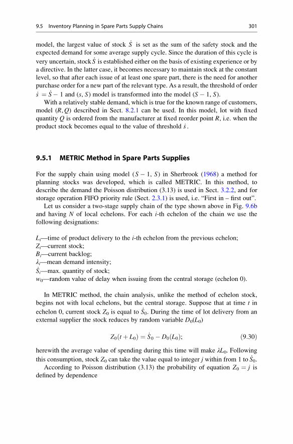
model, the largest value of stock _S is set as the sum of the safety stock and the
expected demand for some average supply cycle. Since the duration of this cycle is
very uncertain, stock _S is established either on the basis of existing experience or by
a directive. In the latter case, it becomes necessary to maintain stock at the constant
level, so that after each issue of at least one spare part, there is the need for another
purchase order for a new part of the relevant type. As a result, the threshold of order
_s ¼ _S� 1 and (s, S) model is transformed into the model (S� 1, S).With a relatively stable demand, which is true for the known range of customers,
model (R,Q) described in Sect. 8.2.1 can be used. In this model, lot with fixed
quantity Q is ordered from the manufacturer at fixed reorder point R, i.e. when the
product stock becomes equal to the value of threshold _s .
9.5.1 METRIC Method in Spare Parts Supplies
For the supply chain using model (S� 1, S) in Sherbrook (1968) a method for
planning stocks was developed, which is called METRIC. In this method, to
describe the demand the Poisson distribution (3.13) is used in Sect. 3.2.2, and for
storage operation FIFO priority rule (Sect. 2.3.1) is used, i.e. “First in – first out”.
Let us consider a two-stage supply chain of the type shown above in Fig. 9.6b
and having N of local echelons. For each i-th echelon of the chain we use the
following designations:
Li—time of product delivery to the i-th echelon from the previous echelon;
Zi—current stock;
Bi—current backlog;
λi—mean demand intensity;_Si—max. quantity of stock;
w0—random value of delay when issuing from the central storage (echelon 0).
In METRIC method, the chain analysis, unlike the method of echelon stock,
begins not with local echelons, but the central storage. Suppose that at time t in
echelon 0, current stock Z0 is equal to _S0. During the time of lot delivery from an
external supplier the stock reduces by random variable D0(L0)
Z0 tþ L0ð Þ ¼ _S0 � D0 L0ð Þ; ð9:30Þherewith the average value of spending during this time will make λL0. Following
this consumption, stock Z0 can take the value equal to integer j within from 1 to _S0.According to Poisson distribution (3.13) the probability of equation Z0 ¼ j is
defined by dependence
9.5 Inventory Planning in Spare Parts Supply Chains 301
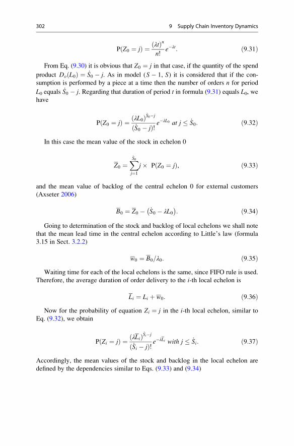
PðZ0 ¼ jÞ ¼ ðλtÞnn!
e�λt: ð9:31Þ
From Eq. (9.30) it is obvious that Z0 ¼ j in that case, if the quantity of the spend
product Do L0ð Þ ¼ _S0 � j. As in model (S� 1, S) it is considered that if the con-
sumption is performed by a piece at a time then the number of orders n for period
L0 equals _S0 � j. Regarding that duration of period t in formula (9.31) equals L0, wehave
PðZ0 ¼ jÞ ¼ ðλL0Þ _S0�j
ð _S0 � jÞ! e�λL0 at j � _S0: ð9:32Þ
In this case the mean value of the stock in echelon 0
Z0 ¼X_S0j¼1
j� PðZ0 ¼ jÞ, ð9:33Þ
and the mean value of backlog of the central echelon 0 for external customers
(Axseter 2006)
B0 ¼ Z0 � _S0 � λL0�
: ð9:34ÞGoing to determination of the stock and backlog of local echelons we shall note
that the mean lead time in the central echelon according to Little’s law (formula
3.15 in Sect. 3.2.2)
w0 ¼ B0=λ0: ð9:35ÞWaiting time for each of the local echelons is the same, since FIFO rule is used.
Therefore, the average duration of order delivery to the i-th local echelon is
Li ¼ Li þ w0: ð9:36ÞNow for the probability of equation Zi ¼ j in the i-th local echelon, similar to
Eq. (9.32), we obtain
PðZi ¼ jÞ ¼ ðλLiÞ _Si�j
ð _Si � jÞ! e�λLi with j � _Si: ð9:37Þ
Accordingly, the mean values of the stock and backlog in the local echelon are
defined by the dependencies similar to Eqs. (9.33) and (9.34)
302 9 Supply Chain Inventory Dynamics

Zi ¼X_Sij¼1
j� PðZi ¼ jÞ and Bi ¼ Zi � ð _Si � λLiÞ: ð9:38Þ
The mean lead time in the local echelon, similarly as in Eq. (9.35)
wi ¼ Bi=λi: ð9:39ÞTable 9.11 shows the input parameters of the supply chain in Fig. 9.6b and the
corresponding mean values of stocks and backlogs as determined by the above
dependencies. Obviously, the intensity of orders in echelon 0 is the sum of the
intensities in echelons 1, 2, 3, and value λ0L0 ¼ 4:8.The mean value of the stock in echelon 0 according to expressions (9.32) and
(9.33)
Z0 ¼X_S0j¼1
j� PðZ0 ¼ jÞ ¼ 1� 4:83
3!þ 2� 4:82
2!þ 3� 4:81
1!þ 4� 4:80
0!
� �e�4:8
¼ 0:493:
Themean value of backlog in echelon 0 fromEq. (9.34)B0 ¼ 0:49�4þ4:8¼ 1:29,and the mean waiting time for order in echelon 0, according to Eq. (9.35)
w0 ¼ 1:29=1:2 ¼ 1:08 day. As a result, the lead time of the order from the central
echelon increases from 1 day to 2.08 days. Results for stocks and backlogs in the
local echelons in Table 9.11 are calculated by formula (9.38). In the cases, where
mean lead timewi of the order is set regulatory, Table 9.11 can be used to determine
the relevant regulatory stocks _S i in each echelon of the chain.
The described method can be used if the order quantity of the central echelon for
an external supplier is greater than unity, i.e. for the order in the form of a lot with
quantity Q. In this case, stock management model (S, Q) (Sect. 8.2.1) is used, inwhich the reorder threshold in echelon 0 is equal to
_s0 ¼ _S0 � Q0: ð9:40ÞThe probability of equation Z0 ¼ j, similarly to Eq. (9.32), has the form (Clark
and Scarf 1960)
Table 9.11 Parameters of the supply chain, mean stocks and backlogs
Echelon λi pcs/day _S i pcs Li days Li days Zi pcs Bi pcs wi days
0 1.2 4 4 – 0.49 1.29 1.08
1 0.1 1 1 2.08 0.81 0.02 0.20
2 0.7 3 1 2.08 1.62 0.08 0.17
3 0.4 2 1 2.08 1.23 0.06 0.16
9.5 Inventory Planning in Spare Parts Supply Chains 303
PðZ0 ¼ jÞ ¼ 1
Q0
X_S0k¼max j, _s 0þ1ð Þ
ðλL0Þk�j
ðk � jÞ! e�λL0 with j � _S0: ð9:41Þ
Assume that with the data in Table 9.11 lot quantity Q0 ¼ 2 and accordingly
_s 0 ¼ 4� 2 ¼ 2. In this case, for example, for j ¼ 1 k ¼ max 1, 2þ 1ð Þ ¼ 3 and
PðZ0 ¼ 1Þ ¼ 1
2
X4k¼3
ð1:2� 4Þk�1
ðk � 1Þ! e�1:2�4 or
PðZ0 ¼ 1Þ ¼ 1
2
ð1:2� 4Þ3�1
ð3� 1Þ! þ ð1:2� 4Þ4�1
ð4� 1Þ!
" #e�4:8 ¼ 0:123:
By calculating in the same way the probabilities of stocks at j ¼ 2, 3, 4, we will
obtain the mean stock in echelon 0 according to Eq. (9.33):
Z0 ¼X_S0j¼1
j� PðZ0 ¼ jÞ ¼ 1� 0:123þ 2� 0:067þ 3� 0:023þ 4� 0:004
¼ 0:35:
Comparing the obtained value with the stock calculated above when the quantity
of the order is equal to unity, we see that the value of the mean stock with increase
in the quantity of the order reduces. In contrast to (S� 1, S) model used in case of
rare and irregular demand, ordering by lots in (S, Q) model is applied at relatively
predictable demand. An example of irregular demand is operation of military
equipment; an example of stable demand for spare parts can be maintenance of
the vehicle fleet. In the latter case, to plan spare parts supply by lots it makes sense
to use DRP-tables described in Sect. 9.1.
In those cases where for maintenance it is required to have n parts of different
types, the mean waiting time for the required set of parts in the i-th local echelon
can be determined using a variation of the above-described method, which is called
MOD-METRIC (Muckstadt and Thomas 1980). The corresponding expression has
the form
wi ¼Xnj¼1
λi, jwi, j=Xnj¼1
λi, j: ð9:42Þ
For example, assume that in echelon 2 (Table 9.11), besides the spare part with
number 1 and intensive demand λ2,1 ¼ 0:7, for the maintenance it is required to
have also spare part 2 with demand intensity λ2,1 ¼ 0:5. The mean waiting time for
part 1, according to Table 9.11, is 0.17. Assume that the waiting time for part 2 is
0.25. Then we obtain
304 9 Supply Chain Inventory Dynamics

wi ¼X2j¼1
λi, jwi, j=X2j¼1
λi, j ¼ 0:7� 0:17þ 0:5� 0:25
0:7þ 0:5¼ 0:2:
9.5.2 Inventory Planning for Central Spare Parts Storage Using(R,Q) Model
Usually, the demand for spare parts is random, and at the same time it requires fast
fulfilment of orders. High level of orders service, of course, necessitates maintaining
large stocks in the distribution storage.At the same time, stocks availability is associated
with significant costs for their keeping.
The article (Hopp et al. 1997) presents the development of a method for optimal
control of the storage, which has a wide range of spare parts, and as a computational
model the so-called (R,Q) model (Sect. 8.2.1) is used. The goal of optimal control
in this case is to minimize the total cost of stocks when there are two constraints: on
mean frequency of orders for replenishment and on mean level of customer service
at the storage.
The method suggested in Hopp et al. (1997) was further developed in Zhang
et al. (2001), and here mainly the results obtained in this paper are given. In
accordance with Zhang et al. (2001) for the i-th type of parts we denote the annual
demand as Di, the cost per nomenclature unit as ci, the lead time as li in years, the
consumption of spare parts during the lead time as θi ¼ Dili, and the number of
items in the nomenclature of parts as n. We also denote the total demand for all
nomenclature items as D ¼Xni¼1
Di and total cost as c ¼Xni¼1
ci.
The probability density of demand distribution is denoted by Pi, and standard
deviation of demand during delivery is denoted as σi. If we assume that the demand
for any type of i-th parts within the shipping time has Poisson distribution (Sect.
3.2.2), then σ2i ¼ θi (Zhang et al. 2001).
For each i-th product, generally speaking, the directive constraint can be set for
the highest frequency of orders Ωi, as well as for own level of customer service SLi.However, in the presence of a large range of spare parts it is possible to set some
average values of these parameters Ω and SL.
The value of the mean stockZi of the i-th type parts depends on order quantity Qi
and reorder threshold _s i
Zi _si;Qið Þ ¼ _s i � θi þ Qi=2: ð9:43ÞIn the strict sense, expression (9.43) is valid if _s � θ � 0, but in Hopp
et al. (1997) it is said that there will be no big error when it is used, if _s � θ < 0.
In this case the optimization problem is finding the minimum of value
9.5 Inventory Planning in Spare Parts Supply Chains 305
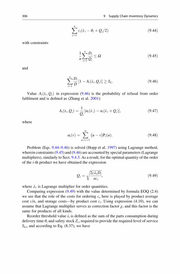
Xni¼1
ci _s i � θi þ Qi=2ð Þ ð9:44Þ
with constraints
1
n
Xni¼1
Di
Qi
� Ω ð9:45Þ
and
Xni¼1
Di
D1� Ai _si;Qið Þ½ � � SL: ð9:46Þ
Value Ai _si;Qið Þ in expression (9.46) is the probability of refusal from order
fulfilment and is defined as (Zhang et al. 2001):
Ai _si;Qið Þ ¼ 1
Qi
αi _s ið Þ � αi _s i þ Qið Þ½ �; ð9:47Þ
where
αiðvÞ ¼X1u¼vþ1
�u� v
PiðuÞ: ð9:48Þ
Problem (Eqs. 9.44–9.46) is solved (Hopp et al. 1997) using Lagrange method,
wherein constraints (9.45) and (9.46) are accounted by special parameters (Lagrange
multipliers), similarly to Sect. 9.4.3. As a result, for the optimal quantity of the order
of the i-th product we have obtained the expression
Qi ¼ffiffiffiffiffiffiffiffiffiffiffiffiffiffi2cλ1Di
nci
r, ð9:49Þ
where λ1 is Lagrange multiplier for order quantities.
Comparing expression (9.49) with the value determined by formula EOQ (2.4)
we see that the role of the costs for ordering co here is played by product average
cost c/n, and storage costs—by product cost ci. Using expression (4.10), we can
assume that Lagrange multiplier serves as correction factor χ, and this factor is the
same for products of all kinds.
Reorder threshold value _si is defined as the sum of the parts consumption during
delivery time θi and safety stock Zci required to provide the required level of serviceSLi, and according to Eq. (8.37), we have
306 9 Supply Chain Inventory Dynamics
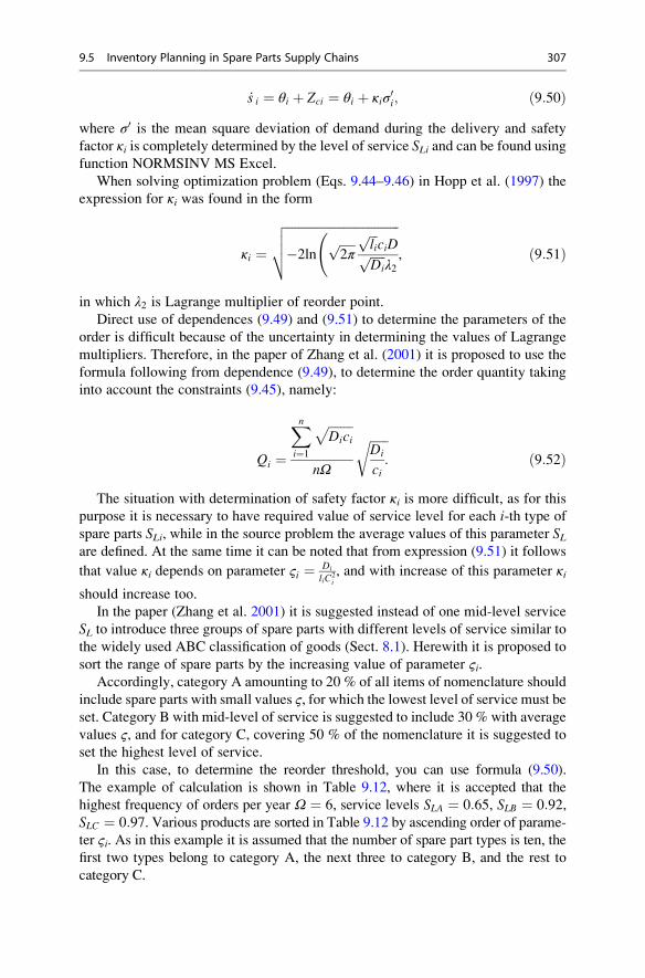
_s i ¼ θi þ Zci ¼ θi þ κiσ0i; ð9:50Þ
where σ0 is the mean square deviation of demand during the delivery and safety
factor κi is completely determined by the level of service SLi and can be found usingfunction NORMSINV MS Excel.
When solving optimization problem (Eqs. 9.44–9.46) in Hopp et al. (1997) the
expression for κi was found in the form
κi ¼ffiffiffiffiffiffiffiffiffiffiffiffiffiffiffiffiffiffiffiffiffiffiffiffiffiffiffiffiffiffiffiffiffiffiffiffiffi�2ln
ffiffiffiffiffi2π
p ffiffiffili
pciDffiffiffiffiffiDi
pλ2
vuut , ð9:51Þ
in which λ2 is Lagrange multiplier of reorder point.
Direct use of dependences (9.49) and (9.51) to determine the parameters of the
order is difficult because of the uncertainty in determining the values of Lagrange
multipliers. Therefore, in the paper of Zhang et al. (2001) it is proposed to use the
formula following from dependence (9.49), to determine the order quantity taking
into account the constraints (9.45), namely:
Qi ¼
Xni¼1
ffiffiffiffiffiffiffiffiDici
pnΩ
ffiffiffiffiffiffiDi
ci:
rð9:52Þ
The situation with determination of safety factor κi is more difficult, as for this
purpose it is necessary to have required value of service level for each i-th type of
spare parts SLi, while in the source problem the average values of this parameter SLare defined. At the same time it can be noted that from expression (9.51) it follows
that value κi depends on parameter ςi ¼ Di
liC2i
, and with increase of this parameter κi
should increase too.
In the paper (Zhang et al. 2001) it is suggested instead of one mid-level service
SL to introduce three groups of spare parts with different levels of service similar to
the widely used ABC classification of goods (Sect. 8.1). Herewith it is proposed to
sort the range of spare parts by the increasing value of parameter ςi.Accordingly, category A amounting to 20 % of all items of nomenclature should
include spare parts with small values ς, for which the lowest level of service must be
set. Category B with mid-level of service is suggested to include 30 % with average
values ς, and for category C, covering 50 % of the nomenclature it is suggested to
set the highest level of service.
In this case, to determine the reorder threshold, you can use formula (9.50).
The example of calculation is shown in Table 9.12, where it is accepted that the
highest frequency of orders per year Ω ¼ 6, service levels SLA ¼ 0:65, SLB ¼ 0:92,SLC ¼ 0:97. Various products are sorted in Table 9.12 by ascending order of parame-
ter ςi. As in this example it is assumed that the number of spare part types is ten, the
first two types belong to category A, the next three to category B, and the rest to
category C.
9.5 Inventory Planning in Spare Parts Supply Chains 307
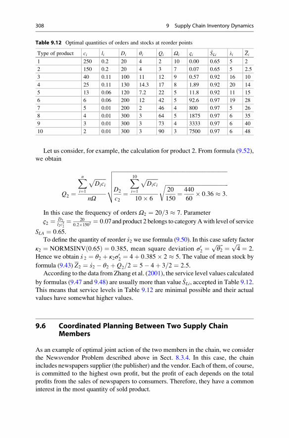
Let us consider, for example, the calculation for product 2. From formula (9.52),
we obtain
Q2 ¼
Xni¼1
ffiffiffiffiffiffiffiffiDici
pnΩ
ffiffiffiffiffiffiffiffiffiffiffiffiffiffiffiffiffiffiffiffiffiffiffiffiffiffiffiffiffiffiffiffiffiffiffiffiffiffiffiffiffiffiffiffiffiffiffiffiffiffiffiffiffiffiffiffiffiffiffiffiffiffiffiffiffiffiffiffiffiffiffiffiffiffiffiffiffiffiffiffiffiffiffiD2
c2¼
X10i¼1
ffiffiffiffiffiffiffiffiDici
p10� 6
ffiffiffiffiffiffiffiffiffiffiffiffiffiffiffiffiffiffiffiffiffiffiffiffiffiffiffiffiffiffiffiffiffiffiffiffiffiffiffiffiffiffiffiffiffiffi20
150¼ 440
60� 0:36 � 3:
rvuuuut
In this case the frequency of orders Ω2 ¼ 20=3 � 7. Parameter
ς2 ¼ D2
l2c22¼ 20
0:2�1502¼ 0:07and product 2 belongs to categoryAwith level of service
SLA ¼ 0:65.To define the quantity of reorder _s2 we use formula (9.50). In this case safety factor
κ2 ¼ NORMSINV 0:65ð Þ ¼ 0:385, mean square deviation σ02 ¼ffiffiffiffiffiθ2
p ¼ ffiffiffi4
p ¼ 2.
Hence we obtain _s 2 ¼ θ2 þ κ2σ02 ¼ 4þ 0:385� 2 � 5. The value of mean stock by
formula (9.43) Z2 ¼ _s2 � θ2 þ Q2=2 ¼ 5� 4þ 3=2 ¼ 2:5.According to the data fromZhang et al. (2001), the service level values calculated
by formulas (9.47 and 9.48) are usually more than value _SLi, accepted in Table 9.12.This means that service levels in Table 9.12 are minimal possible and their actual
values have somewhat higher values.
9.6 Coordinated Planning Between Two Supply ChainMembers
As an example of optimal joint action of the two members in the chain, we consider
the Newsvendor Problem described above in Sect. 8.3.4. In this case, the chain
includes newspapers supplier (the publisher) and the vendor. Each of them, of course,
is committed to the highest own profit, but the profit of each depends on the total
profits from the sales of newspapers to consumers. Therefore, they have a common
interest in the most quantity of sold product.
Table 9.12 Optimal quantities of orders and stocks at reorder points
Type of product ci li Di θi Qi Ωi ςi _SLi _si Zi
1 250 0.2 20 4 2 10 0.00 0.65 5 2
2 150 0.2 20 4 3 7 0.07 0.65 5 2.5
3 40 0.11 100 11 12 9 0.57 0.92 16 10
4 25 0.11 130 14.3 17 8 1.89 0.92 20 14
5 13 0.06 120 7.2 22 5 11.8 0.92 11 15
6 6 0.06 200 12 42 5 92.6 0.97 19 28
7 5 0.01 200 2 46 4 800 0.97 5 26
8 4 0.01 300 3 64 5 1875 0.97 6 35
9 3 0.01 300 3 73 4 3333 0.97 6 40
10 2 0.01 300 3 90 3 7500 0.97 6 48
308 9 Supply Chain Inventory Dynamics
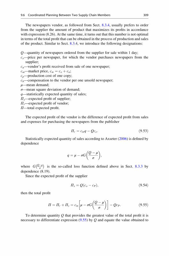
The newspapers vendor, as followed from Sect. 8.3.4, usually prefers to order
from the supplier the amount of product that maximizes its profits in accordance
with expression (8.26). At the same time, it turns out that this number is not optimal
in terms of the total profit that can be obtained in the process of production and sales
of the product. Similar to Sect. 8.3.4, we introduce the following designations:
Q—quantity of newspapers ordered from the supplier for sale within 1 day;
co—price per newspaper, for which the vendor purchases newspapers from the
supplier;
cu—vendor’s profit received from sale of one newspaper;
cm—market price, cm ¼ co þ cu;cp—production cost of one copy;
cb—compensation to the vendor per one unsold newspaper;
μ—mean demand;
σ—mean square deviation of demand;
q—statistically expected quantity of sales;
Πs—expected profit of supplier;
Πr—expected profit of vendor;
Π—total expected profit.
The expected profit of the vendor is the difference of expected profit from sales
and expenses for purchasing the newspapers from the publisher
Πr ¼ cmq� Qco: ð9:53ÞStatistically expected quantity of sales according to Axseter (2006) is defined by
dependence
q ¼ μ� σGQ� μ
σ
� �;
where G Q�μσ
� is the so-called loss function defined above in Sect. 8.3.3 by
dependence (8.19).
Since the expected profit of the supplier
Πs ¼ Q co � cPð Þ; ð9:54Þthen the total profit
Π ¼ Πr þ Πs ¼ cm μ� σGQ� μ
σ
� � �� QcP: ð9:55Þ
To determine quantity Q that provides the greatest value of the total profit it is
necessary to differentiate expression (9.55) by Q and equate the value obtained to
9.6 Coordinated Planning Between Two Supply Chain Members 309
zero, which is the same operation as in Sect. 8.3.4 above. As a result, we obtain the
expression for optimal Q*
ΦQ* � μ
σ
� �¼ co � cp þ cu
cmwith co > cP: ð9:56Þ
However, the vendor orders the quantity of newspapers less than Q* from the
supplier, since for him optimal order quantity Qr is defined by dependence (8.26)
ΦQ*
r � μ
σ
� �¼ cu
cm; ð9:57Þ
the right side of which is obviously less than the right side of expression (9.56).
In order to encourage the vendor to do the order equal to Q*, the supplier must
share a part of its profit. For example, perhaps the supplier can take back the newspapers
unsold during the day with predetermined compensation cb. Let the size of the com-
pensation depend on the market price
cb ¼ 1� gð Þcm; ð9:58Þand the selling price is set in the amount of
c0 ¼ 1� gð Þcm þ gcPwith 0 < g < 1: ð9:59ÞIn this case the vendor’s profit
Πr ¼ cmq� Qco þ cb Q� qð Þ ¼ gcmq� gQco ¼ gΠ; ð9:60Þand the supplier’s profit
Πs ¼ Q co � cPð Þ � cb Q� qð Þ ¼ 1� gð Þcmq� 1� gð ÞQco ¼ 1� gð ÞΠ: ð9:61ÞThus, with coordinated action of the supplier and vendor the optimal order quantity
should be determined from expression (9.56), and the members of the supply chain
must agree on the sharing of common profits, establishing acceptable rate g.Let us consider an example of such calculation using the data from the example
in Sect. 8.3.4, in which μ ¼ 50; σ ¼ 14 and purchasing price co ¼ 10, sales liftup
cu ¼ 15, and cP ¼ 5. From Eq. (9.56) given that cm ¼ co þ cu ¼ 25, we obtain
ΦQ* � 50
14
� �¼ 10� 5þ 15
25¼ 0:8 and NORMSINV 0:8ð Þ ¼ 0:841:
The obtained value Q* � 62 is slightly higher than the optimal quantity of
order of 55 pcs., obtained in Sect. 8.3.4 above by formula (9.57). Suppose, for
example, number of newspapers actually sold q equals mean value μ ¼ 50. In
310 9 Supply Chain Inventory Dynamics
this case the vendor’s profit at his usual not coordinated order is equal to
Πr ¼ 15� 50� 55� 50ð Þ � 10 ¼ 700, and the total profit of the entire chain
amounts to Π ¼ q cm � cPð Þ ¼ 50� 25� 5ð Þ ¼ 1000. Thus, without coordination
the vendor receives 70 % of the profits on average.
It is obvious that coordination is possible only if for each of the members the
coordinated result will not be worse than the result without coordination. Therefore,
offering the vendor to place the order of 62 units, the supplier must agree that the
vendor’s share of the total profit g will be not less than 70 %.
References
Axseter, S. (2006). Inventory control. Berlin: Springer.Cao, D., & Silver, E. A. (2005). A dynamic allocation heuristic for centralized safety stock. Naval
Research Logistics, 52, 513–526.Clark, A., & Scarf, H. (1960). Optimal policies for a multi-echelon inventory problem. Manage-
ment Science, 6, 465–490.Hopp, W. J., Spearmen, M. L., & Zhang, R. Q. (1997). Easily implementable (Q, r) inventory
control policies. Operations Research, 45, 327–340.Lee, H. L., Padmanabhan, V., & Whang, S. (1997a). The bullwhip effect in supply chains. Sloan
Management Review, 38, 93–102.Lee, H. L., Padmanabhan, V., & Whang, S. (1997b). Information distortion in a supply chain: The
Bullwhip effect. Management Science, 43, 546–558.Maister, D. H. (1976). Centralization of inventories and the ‘square root law’. International
Journal of Physical Distribution, 6, 124–134.Muckstadt, J. A., & Thomas, L. J. (1980). Are multi-echelon inventory models worth
implementing in systems with low-demand-rate items? Management Science, 26, 483–494.Nyhuis, P., & Wiendahl, H.-P. (2009). Fundamentals of production logistics. Berlin: Springer.Sachko, N. S. (2008). Organization and operational management of machinery production.
Minsk: Novoe znanie (in Russian).
Sherbrook, C. C. (1968). METRIC: A multi-echelon technique for recoverable item control.
Operations Research, 16, 122–141.Vollmann, T. E., Berry, W. L., Whybark, D. C., & Jacobs, F. R. (2005). Manufacturing planning
and control for supply chain management. Boston: McGraw Hill.
Zhang, R. Q., Hopp, W. J., & Supagiat, C. (2001). Spreadsheet implementable inventory control
for a distribution center. Journal of Heuristics, 7, 185–203.
References 311
Planning of Supplies to Consumers 10
10.1 Sales and Operation Planning
The sales and operations plan is elaborated according to the business plan or similar
document describing the enterprise development strategy and is the basis for its
operations. This plan connects the main goals of the business plan with planning of
production, finance, sales, and other enterprise services.
10.1.1 Interrelation Between Various Planning Directions with Salesand Operations Plan
Figure 10.1 shows the basic planning directions related to the sales and operations
plan. As can be seen from Fig. 10.1, the indices of this plan are generated based on a
range of figures determined during strategic planning, demand planning, and finance
planning as well as the constraints set during planning of production, procurement,
and sales.
The input data for sales and operations planning are key figures of output of the
main aggregated types of products, defined in strategic planning, and demand fore-
casting results for these products. During plan elaboration, these data are analysed
and compared with the available resources.
The quality of the sales and operations plan under development is primarily
determined by the balance of demand for products and resources used. If the demand
exceeds the capabilities of the enterprise significantly during its normal operation,
this leads to an increase in cost due to overtime payments and a reduction in the
product quality. On the contrary, when the production plan is in excess of actual
demand, it causes surplus products and financial and economic indicators decline.
Another very important aspect of the sales and operations plan consists in the
right ratio of the aggregate products planning and its detailing. In developing the
sales and operations plan, first it is necessary to define the consolidated production
# Springer International Publishing Switzerland 2016
Y. Mauergauz, Advanced Planning and Scheduling in Manufacturing and SupplyChains, DOI 10.1007/978-3-319-27523-9_10
313

output for aggregated groups of products and only then to specify such groups by
specific standard sizes of products.
The need for mandatory planning of aggregated groups is due to the fact that the
adequate balancing of demand and production for an extended period can only be
at the aggregate level. The plan drawn up at this level is the basis of medium-term
planning of material and manpower resources.
The plan by the aggregated product groups can be calculated in different units.
The most common indicator is, of course, the production output in terms of value.
This figure, however, says little to production managers and employees of procure-
ment services. For these employees, for example, values of output in physical units,
tons, or even in labour hours are more convenient.
The amount of aggregated groups are generally (Vollmann et al. 2005) is in the
range from 6 to 12. This grouping allows covering the main types of products and
duly analysing their contribution to the earned income, production, and resources
use. Aggregation of production into groups can be carried out by various parameters:
type of product, size or properties, market segments, and even individual consumers,
etc. The most frequent and successful aggregation is by commodity groups in the
market.
The production plan by a group in a certain period does not necessarily equal
the forecasted demand in this period. The output in some period may provide the
demand of future periods and can less be for some reason than the current demand.
The practice has proven that absence of aggregate sales and operations plan or poor
elaboration of it causes a number of unpleasant consequences—excessive com-
modity and material stocks, low level of customer service, equipment downtime,
long duration of the production cycle, nervousness occurring when dispatching,
overspending of payroll, and finally great difficulties in introducing new products.
Strategic planning
Sales and
operations plan
Finance planning
Demand
planning
Master planSales plan
Procurement plan
Plan for utilization of equipment
Manpower plan
Fig. 10.1 Interactions of various planning directions
314 10 Planning of Supplies to Consumers
10.1.2 Sales and Operation Planning Methods
Themost commonway of sales and operations planning is to draw up tables containing
the values of the correspondingparameters at different time intervals—usuallymonthly
(Table 10.1).
In the example shown in Table 10.1, the sales and operations plan is made on a
quarterly basis with a horizon of 6 months. Here you can see a version of the plan
for the second and third quarters for some aggregated group of products, which are
measured in pieces. According to the last quarter actual sales trends and their devia-
tion from the original plan can be judged. Similarly, we can analyse the results of the
production for the last quarter. In the above example, the increase in production and
the tendency to fulfil the plan are clearly observed.
The main indicator of the production plan is the value of the planned monthly
operating load. Table 10.1 assumes that manufacturing of a product unit of this group
requires 12 h. Considering that the production plan uses the chase strategy, in which
the production should accurately track the demand, the production load varies quite
widely—from 3360 to 4320 h. Accordingly, the average daily load varies as well—
from 156 to 206 h.
The targets stock at the end of each period is usually set by the standard stock
in the days of consumption. In this case, it is assumed that for the product group in
question for the standard is about 8 working days. The actual stock in days for each
of the last periods can be determined by dividing the available balance by con-
sumption rate during this period.
Consistent use of the chase strategy leads to the necessity of frequent dismissals
or, vice versa, urgent recruitment. Although when integrating of sales and operations
plans of all aggregated product groups produced by the enterprise, the total operating
capacity fluctuations can be reduced, yet the use of the chase strategy in its pure form
occurs rarely. Another extreme strategy of the preparation of a production plan is to
maintain stable level of production (level strategy). In this case, the actual changes in
demand are ignored, and as a result, either stocks increase or consumers’ orders are
not fulfilled accordingly. This strategy, of course, cannot be used long enough.
Actually, the production plan, as a rule, is a compromise between the desire to
produce products in accordance with the forecasted demand and the real capabilities
of the enterprise. First of all, when planning sales and production it makes sense to
establish a rational relationship between the cost of changes in personnel and the cost
of keeping stock balances. To do this, you can consider several plan options and
carry out their ranking by value of total expenses. Besides, it is necessary to take
into account possible both legal and professional consequences of dismissals of
employees, as well as the influence of these factors on the strategic goals of the
enterprise.
The production plan option is acceptable if it can be provided by necessary
resources. Checking of resources use, for the most part, is reduced to approximate
calculations of capacity utilization, but in some cases, it is also necessary to check
10.1 Sales and Operation Planning 315
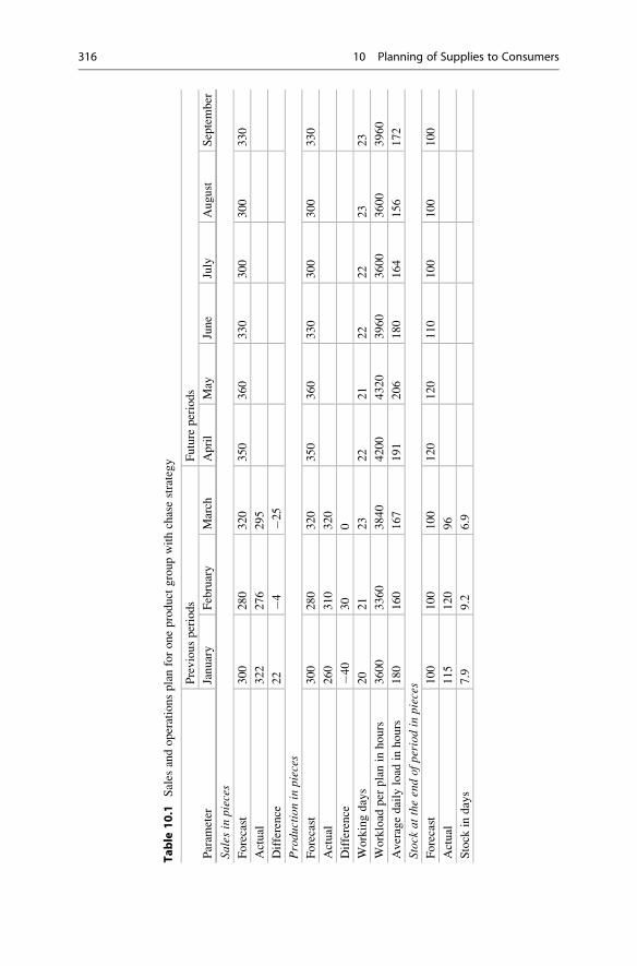
Table
10.1
Sales
andoperationsplanforoneproduct
groupwithchasestrategy
Param
eter
Previousperiods
Future
periods
January
February
March
April
May
June
July
August
September
Sales
inpieces
Forecast
300
280
320
350
360
330
300
300
330
Actual
322
276
295
Difference
22
�4�2
5
Production
inpieces
Forecast
300
280
320
350
360
330
300
300
330
Actual
260
310
320
Difference
�40
30
0
Workingdays
20
21
23
22
21
22
22
23
23
Workload
per
planin
hours
3600
3360
3840
4200
4320
3960
3600
3600
3960
Averagedaily
load
inhours
180
160
167
191
206
180
164
156
172
Stock
attheendofperiodin
pieces
Forecast
100
100
100
120
120
110
100
100
100
Actual
115
120
96
Stock
indays
7.9
9.2
6.9
316 10 Planning of Supplies to Consumers
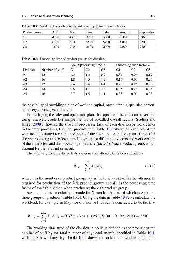
the possibility of providing a plan of working capital, raw materials, qualified person-
nel, energy, water, vehicles, etc.
In developing the sales and operations plan, the capacity utilization can be verified
using relatively crude but simple method of so-called overall factors (Stadtler and
Kilger 2008), showing the share of processing time of each division or work center
in the total processing time per product unit. Table 10.2 shows an example of the
workload calculated for certain version of the sales and operations plan. Table 10.3
shows processing time of each product group for different divisions and work centers
of the enterprise, and the processing time share (factor) of each product group, which
account for the relevant division.
The capacity load of the i-th division in the j-th month is determined as
Wij ¼Xnk¼1
KikWjk; ð10:1Þ
where n is the number of product group;Wjk is the total workload in the j-th month,
required for production of the k-th product group; and Kik is the processing time
factor of the i-th division when producing the k-th product group.
Assume that the calculation is made for 6 months, the first of which is April, on
three groups of products (Table 10.2). Using the data in Table 10.3, we calculate the
workload, for example in May, for division A1, which is considered to be the first
W1,2 ¼X3k¼1
K1kW2k ¼ 0:37� 4320þ 0:26� 5100þ 0:19� 2100 ¼ 3340:
The working time fund of the division in hours is defined as the product of the
number of staff by the total number of days each month, specified in Table 10.1,
with an 8-h working day. Table 10.4 shows the calculated workload in hours
Table 10.2 Workload according to the sales and operations plan in hours
Product group April May June July August September
G1 4200 4320 3960 3600 3600 3960
G2 6300 5100 5500 5400 5400 6200
G3 1800 2100 2100 2300 2300 2400
Table 10.3 Processing time of product groups for divisions
Division Number of staff
Group processing time, h Processing time factor K
G1 G2 G3 G1 G2 G3
A1 23 4.5 1.3 0.9 0.37 0.26 0.19
A2 16 1.8 0.5 1.2 0.15 0.10 0.25
A3 12 2.4 0.6 0.4 0.20 0.12 0.08
A4 14 0.6 1.1 1.2 0.05 0.22 0.25
A5 16 2.7 1.5 1.1 0.23 0.30 0.23
10.1 Sales and Operation Planning 317
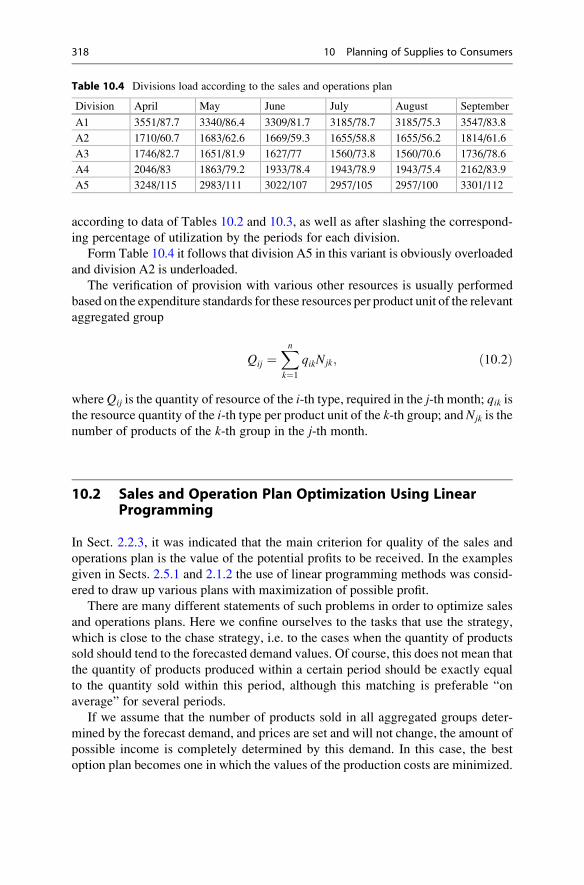
according to data of Tables 10.2 and 10.3, as well as after slashing the correspond-
ing percentage of utilization by the periods for each division.
Form Table 10.4 it follows that division A5 in this variant is obviously overloaded
and division A2 is underloaded.
The verification of provision with various other resources is usually performed
based on the expenditure standards for these resources per product unit of the relevant
aggregated group
Qij ¼Xnk¼1
qikNjk; ð10:2Þ
whereQij is the quantity of resource of the i-th type, required in the j-th month; qik isthe resource quantity of the i-th type per product unit of the k-th group; and Njk is the
number of products of the k-th group in the j-th month.
10.2 Sales and Operation Plan Optimization Using LinearProgramming
In Sect. 2.2.3, it was indicated that the main criterion for quality of the sales and
operations plan is the value of the potential profits to be received. In the examples
given in Sects. 2.5.1 and 2.1.2 the use of linear programming methods was consid-
ered to draw up various plans with maximization of possible profit.
There are many different statements of such problems in order to optimize sales
and operations plans. Here we confine ourselves to the tasks that use the strategy,
which is close to the chase strategy, i.e. to the cases when the quantity of products
sold should tend to the forecasted demand values. Of course, this does not mean that
the quantity of products produced within a certain period should be exactly equal
to the quantity sold within this period, although this matching is preferable “on
average” for several periods.
If we assume that the number of products sold in all aggregated groups deter-
mined by the forecast demand, and prices are set and will not change, the amount of
possible income is completely determined by this demand. In this case, the best
option plan becomes one in which the values of the production costs are minimized.
Table 10.4 Divisions load according to the sales and operations plan
Division April May June July August September
A1 3551/87.7 3340/86.4 3309/81.7 3185/78.7 3185/75.3 3547/83.8
A2 1710/60.7 1683/62.6 1669/59.3 1655/58.8 1655/56.2 1814/61.6
A3 1746/82.7 1651/81.9 1627/77 1560/73.8 1560/70.6 1736/78.6
A4 2046/83 1863/79.2 1933/78.4 1943/78.9 1943/75.4 2162/83.9
A5 3248/115 2983/111 3022/107 2957/105 2957/100 3301/112
318 10 Planning of Supplies to Consumers
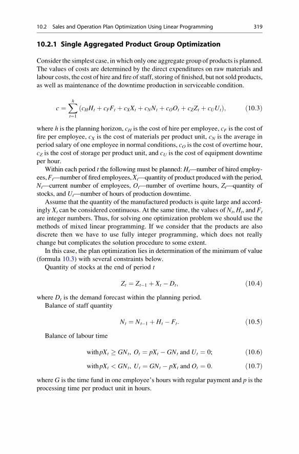
10.2.1 Single Aggregated Product Group Optimization
Consider the simplest case, in which only one aggregate group of products is planned.
The values of costs are determined by the direct expenditures on raw materials and
labour costs, the cost of hire and fire of staff, storing of finished, but not sold products,
as well as maintenance of the downtime production in serviceable condition.
c ¼Xht¼1
cHHt þ cFFt þ cXXt þ cNNt þ cOOt þ cZZt þ cUUtð Þ; ð10:3Þ
where h is the planning horizon, cH is the cost of hire per employee, cF is the cost offire per employee, cX is the cost of materials per product unit, cN is the average in
period salary of one employee in normal conditions, cO is the cost of overtime hour,
cZ is the cost of storage per product unit, and cU is the cost of equipment downtime
per hour.
Within each period t the following must be planned:Ht—number of hired employ-
ees,Ft—number of fired employees,Xt—quantity of product producedwith the period,
Nt—current number of employees, Ot—number of overtime hours, Zt—quantity of
stocks, and Ut—number of hours of production downtime.
Assume that the quantity of the manufactured products is quite large and accord-
ingly Xt can be considered continuous. At the same time, the values of Nt, Ht, and Ft
are integer numbers. Thus, for solving one optimization problem we should use the
methods of mixed linear programming. If we consider that the products are also
discrete then we have to use fully integer programming, which does not really
change but complicates the solution procedure to some extent.
In this case, the plan optimization lies in determination of the minimum of value
(formula 10.3) with several constraints below.
Quantity of stocks at the end of period t
Zt ¼ Zt�1 þ Xt � Dt; ð10:4Þwhere Dt is the demand forecast within the planning period.
Balance of staff quantity
Nt ¼ Nt�1 þ Ht � Ft: ð10:5ÞBalance of labour time
withpXt � GNt, Ot ¼ pXt � GNt and Ut ¼ 0; ð10:6ÞwithpXt < GNt, Ut ¼ GNt � pXt and Ot ¼ 0: ð10:7Þ
where G is the time fund in one employee’s hours with regular payment and p is theprocessing time per product unit in hours.
10.2 Sales and Operation Plan Optimization Using Linear Programming 319
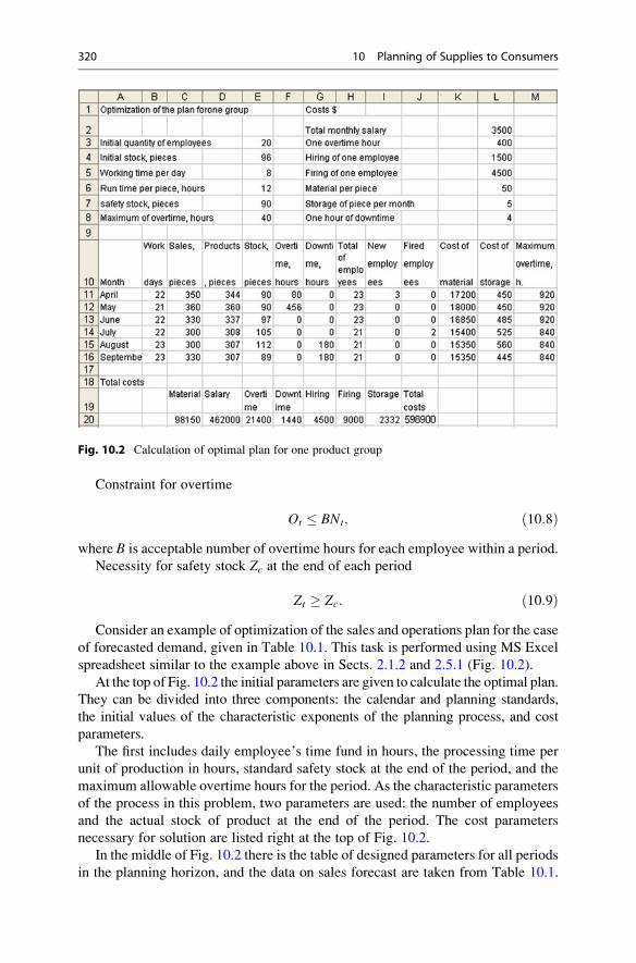
Constraint for overtime
Ot � BNt; ð10:8Þwhere B is acceptable number of overtime hours for each employee within a period.
Necessity for safety stock Zc at the end of each period
Zt � Zc: ð10:9ÞConsider an example of optimization of the sales and operations plan for the case
of forecasted demand, given in Table 10.1. This task is performed using MS Excel
spreadsheet similar to the example above in Sects. 2.1.2 and 2.5.1 (Fig. 10.2).
At the top of Fig. 10.2 the initial parameters are given to calculate the optimal plan.
They can be divided into three components: the calendar and planning standards,
the initial values of the characteristic exponents of the planning process, and cost
parameters.
The first includes daily employee’s time fund in hours, the processing time per
unit of production in hours, standard safety stock at the end of the period, and the
maximum allowable overtime hours for the period. As the characteristic parameters
of the process in this problem, two parameters are used: the number of employees
and the actual stock of product at the end of the period. The cost parameters
necessary for solution are listed right at the top of Fig. 10.2.
In the middle of Fig. 10.2 there is the table of designed parameters for all periods
in the planning horizon, and the data on sales forecast are taken from Table 10.1.
Fig. 10.2 Calculation of optimal plan for one product group
320 10 Planning of Supplies to Consumers
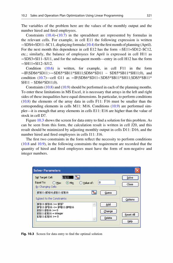
The variables of the problem here are the values of the monthly output and the
number hired and fired employees.
Constraints (10.4)–(10.7) in the spreadsheet are represented by formulas in
the relevant cells. For example, in cell E11 the following expression is written
¼$D$4+$D11–$C11, displaying formula (10.4) for thefirstmonth of planning (April).
For the next month this dependence in cell E12 has the form ¼$E11+$D12–$C12,
etc.; similarly, the balance of employees for April is expressed in cell H11 as
¼$D$3+$I11–$J11, and for the subsequent month—entry in cell H12 has the form
¼$H11+$I12–$J12.
Condition (10.6) is written, for example, in cell F11 in the form
¼IF($D$6*$D11>¼$D$5*$B11*$H11;$D$6*$D11 – $D$5*$B11*$H11;0), and
condition (10.7)—cell G11 as ¼IF($D$6*$D11<$D$5*$B11*$H11;$D$5*$B11*
$H11 – $D$6*$D11;0).
Constraints (10.8) and (10.9) should be performed in each of the planning months.
To enter these limitations in MS Excel, it is necessary that arrays in the left and right
sides of these inequalities have equal dimensions. In particular, to perform conditions
(10.8) the elements of the array data in cells F11: F16 must be smaller than the
corresponding elements in cells M11: M16. Conditions (10.9) are performed sim-
pler—it is enough that array elements in cells E11: E16 are higher than the value of
stock in cell D7.
Figure 10.3 shows the screen for data entry to find a solution for this problem. As
can be seen from this form, the calculation result is written in cell J20, and this
result should be minimized by adjusting monthly output in cells D11: D16, and the
number hired and fired employees in cells I11: J16.
The first two constraints in the form reflect the necessity to perform conditions
(10.8 and 10.9), in the following constraints the requirement are recorded that the
quantity of hired and fired employees must have the form of non-negative and
integer numbers.
Fig. 10.3 Screen for data entry to find the optimal solution
10.2 Sales and Operation Plan Optimization Using Linear Programming 321

In the problem of linear continuous optimization, the example of which is given
above in Sect. 2.1.2, the solution appears to be exact and can be analysed by a
sensitivity report (Fig. 2.4). Integer optimization gives an approximate solution, the
results of which may depend on the initial values of variables. Unfortunately, the
sensitivity report for the problems with integer variables are not provided by MS
Excel.
10.2.2 More Complex Case of Optimization of Salesand Operations Plan
Consider the case of optimizing with parallel production of n product groups and thescale of the planned production is limited by capacity of one work center (division).
As it was mentioned in the previous paragraph, the objective function, in general, is
the received profit. Therefore, we will seek the set of independent variables of the
problem at a planning horizon h, which provide the highest possible amount of
profit. Instead of expression (10.3) the objective function takes the form
Π ¼Xni¼1
Xht¼1
cqiqi, t � cXiXi, t � cZiZi, t
� � hcp�
�Xht¼1
cHHt þ cFFt þ cNNt þ cOOt þ cUUtð Þ;ð10:10Þ
where cqi is the product price of the i-th group, qi,t is the sales volumes of products
of the i-th group during period t, and cp is the constant expenditure within the
period. The rest of the values match the designations in Sect. 10.2.1; at that the cost
of the materials per product unit cXi and the storage cost of product unit cZi dependon the i-th product group. So for each group output Xi,t and storage Zi,t are different.
The appearance of the capacity constraints can cause a reduction in the planned
sales compared with the forecasting demand values. The value of the stock at the
end of period t for each group is defined by the dependence
Zi, t ¼ Zi, t�1 þ Xi, t � qi, t; ð10:11Þand the requirement for safety stock Zc at the end of each period
Zi, t � Zci: ð10:12ÞConstraint (10.5), related to the staff balance, is maintained. Constraints of labour
time balance (10.6) and (10.7) take the form
322 10 Planning of Supplies to Consumers
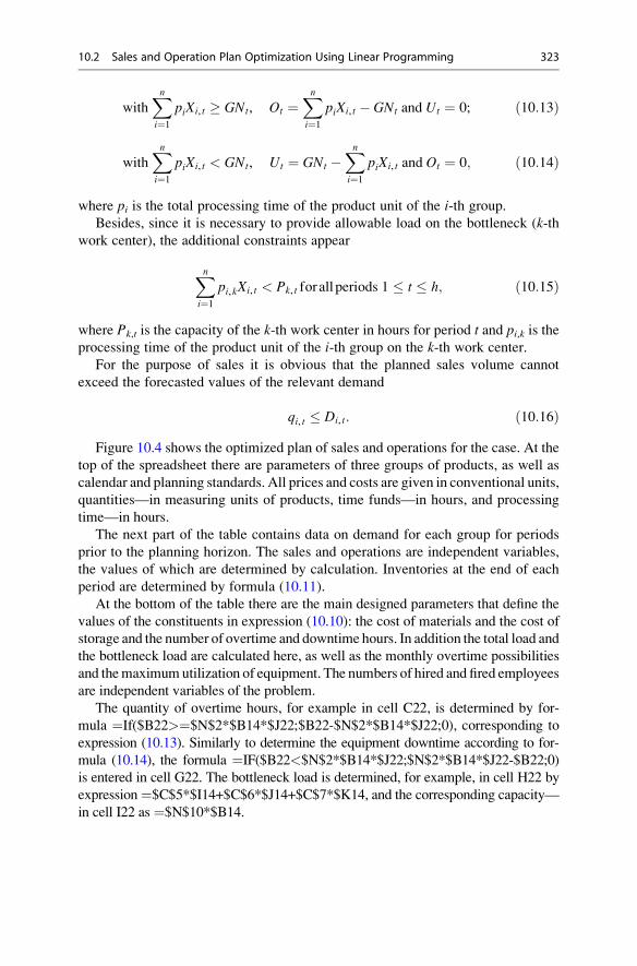
withXni¼1
piXi, t � GNt, Ot ¼Xni¼1
piXi, t � GNt and Ut ¼ 0; ð10:13Þ
withXni¼1
piXi, t < GNt, Ut ¼ GNt �Xni¼1
piXi, t and Ot ¼ 0; ð10:14Þ
where pi is the total processing time of the product unit of the i-th group.
Besides, since it is necessary to provide allowable load on the bottleneck (k-thwork center), the additional constraints appear
Xni¼1
pi,kXi, t < Pk, t forall periods 1 � t � h; ð10:15Þ
where Pk,t is the capacity of the k-th work center in hours for period t and pi,k is theprocessing time of the product unit of the i-th group on the k-th work center.
For the purpose of sales it is obvious that the planned sales volume cannot
exceed the forecasted values of the relevant demand
qi, t � Di, t: ð10:16ÞFigure 10.4 shows the optimized plan of sales and operations for the case. At the
top of the spreadsheet there are parameters of three groups of products, as well as
calendar and planning standards. All prices and costs are given in conventional units,
quantities—in measuring units of products, time funds—in hours, and processing
time—in hours.
The next part of the table contains data on demand for each group for periods
prior to the planning horizon. The sales and operations are independent variables,
the values of which are determined by calculation. Inventories at the end of each
period are determined by formula (10.11).
At the bottom of the table there are the main designed parameters that define the
values of the constituents in expression (10.10): the cost of materials and the cost of
storage and the number of overtime and downtime hours. In addition the total load and
the bottleneck load are calculated here, as well as the monthly overtime possibilities
and themaximumutilization of equipment. The numbers of hired and fired employees
are independent variables of the problem.
The quantity of overtime hours, for example in cell C22, is determined by for-
mula ¼If($B22>¼$N$2*$B14*$J22;$B22-$N$2*$B14*$J22;0), corresponding to
expression (10.13). Similarly to determine the equipment downtime according to for-
mula (10.14), the formula ¼IF($B22<$N$2*$B14*$J22;$N$2*$B14*$J22-$B22;0)
is entered in cell G22. The bottleneck load is determined, for example, in cell H22 by
expression¼$C$5*$I14+$C$6*$J14+$C$7*$K14, and the corresponding capacity—
in cell I22 as ¼$N$10*$B14.
10.2 Sales and Operation Plan Optimization Using Linear Programming 323
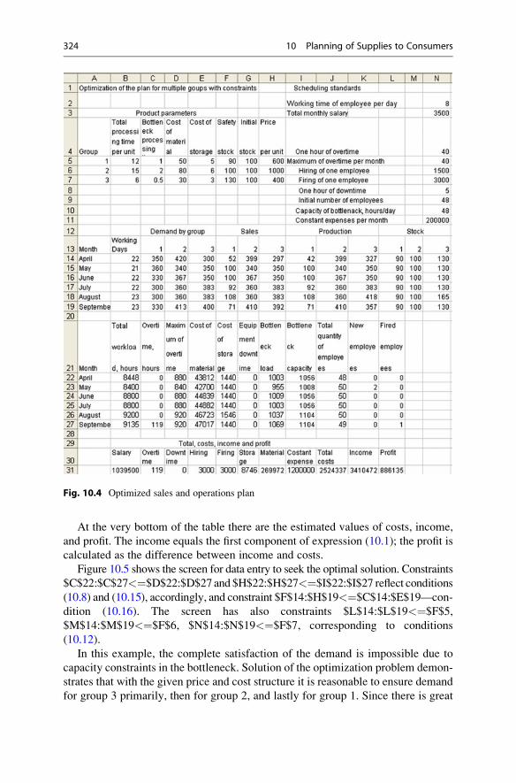
At the very bottom of the table there are the estimated values of costs, income,
and profit. The income equals the first component of expression (10.1); the profit is
calculated as the difference between income and costs.
Figure 10.5 shows the screen for data entry to seek the optimal solution. Constraints
$C$22:$C$27<¼$D$22:$D$27 and $H$22:$H$27<¼$I$22:$I$27 reflect conditions
(10.8) and (10.15), accordingly, and constraint $F$14:$H$19<¼$C$14:$E$19—con-
dition (10.16). The screen has also constraints $L$14:$L$19<¼$F$5,
$M$14:$M$19<¼$F$6, $N$14:$N$19<¼$F$7, corresponding to conditions
(10.12).
In this example, the complete satisfaction of the demand is impossible due to
capacity constraints in the bottleneck. Solution of the optimization problem demon-
strates that with the given price and cost structure it is reasonable to ensure demand
for group 3 primarily, then for group 2, and lastly for group 1. Since there is great
Fig. 10.4 Optimized sales and operations plan
324 10 Planning of Supplies to Consumers
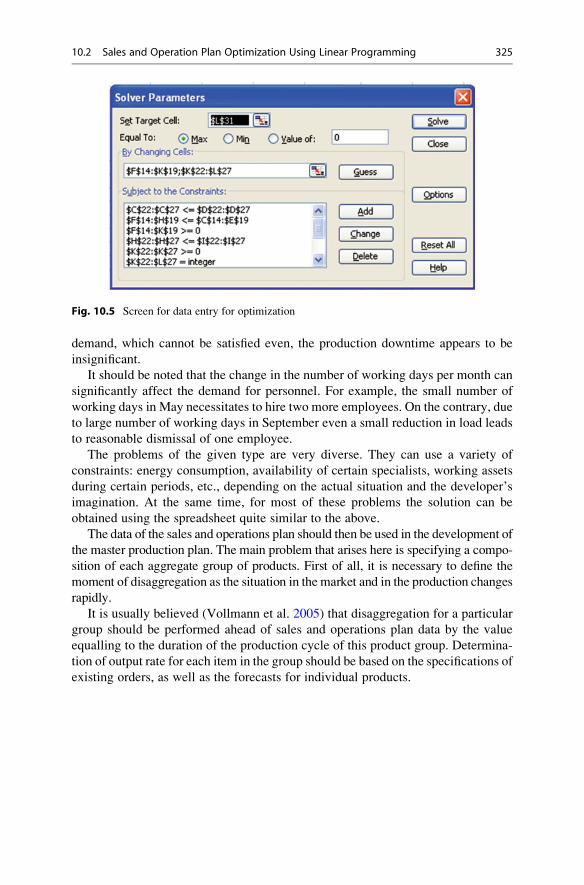
demand, which cannot be satisfied even, the production downtime appears to be
insignificant.
It should be noted that the change in the number of working days per month can
significantly affect the demand for personnel. For example, the small number of
working days in May necessitates to hire two more employees. On the contrary, due
to large number of working days in September even a small reduction in load leads
to reasonable dismissal of one employee.
The problems of the given type are very diverse. They can use a variety of
constraints: energy consumption, availability of certain specialists, working assets
during certain periods, etc., depending on the actual situation and the developer’s
imagination. At the same time, for most of these problems the solution can be
obtained using the spreadsheet quite similar to the above.
The data of the sales and operations plan should then be used in the development of
the master production plan. The main problem that arises here is specifying a compo-
sition of each aggregate group of products. First of all, it is necessary to define the
moment of disaggregation as the situation in the market and in the production changes
rapidly.
It is usually believed (Vollmann et al. 2005) that disaggregation for a particular
group should be performed ahead of sales and operations plan data by the value
equalling to the duration of the production cycle of this product group. Determina-
tion of output rate for each item in the group should be based on the specifications of
existing orders, as well as the forecasts for individual products.
Fig. 10.5 Screen for data entry for optimization
10.2 Sales and Operation Plan Optimization Using Linear Programming 325

10.3 Customized Reservation of Products
The receipt of proposals for a new order by the contractor requires the latter to perform
a series of actions that form the so-called demand fulfilment process. The purpose of
this process is to find out the possibility in principle of the order fulfilment, to calculate
its cost and definition of the probable due date. In the simplest case, when the order is
made on serial products with a known price, the process of accepting the order is
reduced to determining the date of complete fulfilment of the order or the schedule of
its consistent fulfilment.
The conventional approach to this problem is to check the availability of the
product required by the customer at the storage and, then, if the product is available
in the required quantity, it is reserved for the new order; otherwise, the deficiency is
determined, for which the order must be put into production or placed to external
supplier. However, the direct transfer of the order into production is not always
possible, because production capability may be limited to a number of reasons—
equipment load, materials shortages, lack of staff, etc. As a result, it becomes difficult
to get a quick response to a query about the possible due date.
10.3.1 Business Process of Response to New Orders
Modern production management systems provide special business function for
determination of the ability to fulfil the incoming order, which is called Available-
to-Promise (ATP) function. The result of this function is calculation of the neces-
sary amount of the product for the order and the date of its actual fulfilment.
Depending on the required due date of the new order, in the general case, there
may be four different options of a planned situation:
– there is no sales and operations plan for the required due date yet;
– the sales and operations plan is made, but there is no master production plan;
– the master production plan is made, but its implementation is not started yet;
– the master production plan is under way.
In the first case, the feasibility of the order is determined mainly only by the
enterprise development strategy and financial capabilities. Consideration of this
option applies to business planning and is beyond the scope of this book.
Both the first and the second cases, when the order should be fulfilled in the period,
for which the master plan has not yet been developed, are preferred for the manufac-
turer. Since the sales and operations plan is mainly based on demand forecasts, and
covers quite a large horizon, it provides a great opportunity for varying the outputs
and due dates of production. In this case, the check of possibility and feasibility of the
order can be performed by calculating a new plan considering this order.
If the master plan for the period, which should contain the required due date of
the new order, has already been drafted but its implementation has not yet begun,
326 10 Planning of Supplies to Consumers
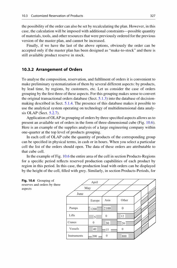
the possibility of the order can also be set by recalculating the plan. However, in this
case, the calculation will be imposed with additional constraints—possible quantity
of materials, tools, and other resources that were previously ordered for the previous
version of the master plan, and cannot be increased.
Finally, if we have the last of the above options, obviously the order can be
accepted only if the master plan has been designed as “make-to-stock” and there is
still available product reserve in stock.
10.3.2 Arrangement of Orders
To analyse the composition, reservation, and fulfilment of orders it is convenient to
make preliminary systematization of them by several different aspects: by products,
by lead time, by regions, by customers, etc. Let us consider the case of orders
grouping by the first three of these aspects. For this grouping makes sense to convert
the original transactional orders database (Sect. 5.1.3) into the database of decision-
making described in Sect. 5.1.4. The presence of this database makes it possible to
use the analytical system operating on technology of multidimensional data analy-
sis OLAP (Sect. 5.2.7).
Application of OLAP in grouping of orders by three specified aspects allows us to
present an available set of orders in the form of three-dimensional cube (Fig. 10.6).
Here is an example of the supplies analysis of a large engineering company within
one-quarter at the top level of products grouping.
In each cell of OLAP cube the quantity of products of the corresponding group
can be specified in physical terms, in cash or in hours. When you select a particular
cell the list of the orders should open. The data of these orders are attributable to
that cube cell.
In the example of Fig. 10.6 the entire area of the cell in section Products-Regions
for a specific period reflects reserved production capabilities of each product by
region in this period. In this case, the production load with orders can be displayed
by the height of the cell, filled with grey. Similarly, in section Products-Periods, for
May
April
June
Pumps
Lifts
Cranes
Vessels
Instruments
Europe Asia Other
0
0
0
0
0
2100
5 12
30 20
40 15
200 800
1200
Fig. 10.6 Grouping of
reserves and orders by three
aspects
10.3 Customized Reservation of Products 327
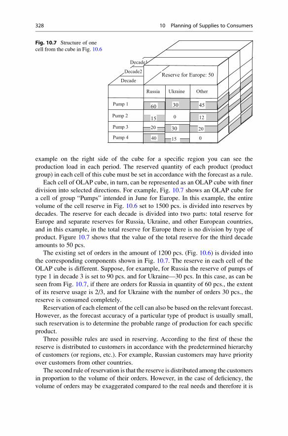
example on the right side of the cube for a specific region you can see the
production load in each period. The reserved quantity of each product (product
group) in each cell of this cube must be set in accordance with the forecast as a rule.
Each cell of OLAP cube, in turn, can be represented as an OLAP cube with finer
division into selected directions. For example, Fig. 10.7 shows an OLAP cube for
a cell of group “Pumps” intended in June for Europe. In this example, the entire
volume of the cell reserve in Fig. 10.6 set to 1500 pcs. is divided into reserves by
decades. The reserve for each decade is divided into two parts: total reserve for
Europe and separate reserves for Russia, Ukraine, and other European countries,
and in this example, in the total reserve for Europe there is no division by type of
product. Figure 10.7 shows that the value of the total reserve for the third decade
amounts to 50 pcs.
The existing set of orders in the amount of 1200 pcs. (Fig. 10.6) is divided into
the corresponding components shown in Fig. 10.7. The reserve in each cell of the
OLAP cube is different. Suppose, for example, for Russia the reserve of pumps of
type 1 in decade 3 is set to 90 pcs. and for Ukraine—30 pcs. In this case, as can be
seen from Fig. 10.7, if there are orders for Russia in quantity of 60 pcs., the extent
of its reserve usage is 2/3, and for Ukraine with the number of orders 30 pcs., the
reserve is consumed completely.
Reservation of each element of the cell can also be based on the relevant forecast.
However, as the forecast accuracy of a particular type of product is usually small,
such reservation is to determine the probable range of production for each specific
product.
Three possible rules are used in reserving. According to the first of these the
reserve is distributed to customers in accordance with the predetermined hierarchy
of customers (or regions, etc.). For example, Russian customers may have priority
over customers from other countries.
The second rule of reservation is that the reserve is distributed among the customers
in proportion to the volume of their orders. However, in the case of deficiency, the
volume of orders may be exaggerated compared to the real needs and therefore it is
Decade2
Decade1
Decade
Pump 1
Pump 2
Pump 3
Pump 4
Russia Ukraine Other
0
0
60 30
15 12
30 20
40 15
45
20
Reserve for Europe: 50
Fig. 10.7 Structure of one
cell from the cube in Fig. 10.6
328 10 Planning of Supplies to Consumers
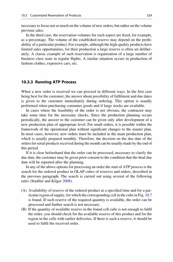
necessary to focus not so much on the volume of new orders, but rather on the volume
previous sales.
In the third case, the reservation volumes for each aspect are fixed, for example,
as a percentage. The volume of the established reserve may depend on the profit-
ability of a particular product. For example, although the high-quality products have
limited sales opportunities, for their production a large reserve is often set deliber-
ately. A classic example of such reservation is organization of a large number of
business class seats in regular flights. A similar situation occurs in production of
fashion clothes, expensive cars, etc.
10.3.3 Running ATP Process
When a new order is received we can proceed in different ways. In the first case
being best for the customer, the answer about possibility of fulfilment and due dates
is given to the customer immediately during ordering. This option is usually
performed when purchasing consumer goods and if large stocks are available.
In cases where the feasibility of the order is not obvious, the contractor may
take some time for the necessary checks. Since the production planning occurs
periodically, the answer to the customer can be given only after development of a
new production plan of appropriate level. For small orders, it is possible within the
framework of the operational plan without significant changes to the master plan.
In most cases, however, new orders must be included in the main production plan,
which is usually prepared monthly. Therefore, the decision on the due date of the
orders for serial products received during themonth can be usuallymade by the end of
this period.
If it is clear beforehand that the order can be processed, necessary to clarify the
due date, the customer may be given prior consent to the condition that the final due
date will be reported after the planning.
In any of the above options for processing an order the start of ATP process is the
search for the ordered product in OLAP cubes of reserves and orders, described in
the previous paragraph. The search is carried out using several of the following
rules (Stadtler and Kilger 2008).
(A) Availability of reserve of the ordered product at a specified time and for a par-
ticular region of supply, for which the corresponding cell in the cube in Fig. 10.7
is found. If such reserve of the required quantity is available, the order can be
processed and further search is not necessary.
(B) If the quantity of available reserve in the found cell cube is not enough to fulfil
the order, you should check for the available reserve of this product and for the
region in the cells with earlier deliveries. If there is such a reserve, it should be
used to fulfil the received order.
10.3 Customized Reservation of Products 329

(C) In the case where after step (B) the existing reserve is insufficient, go to search
the ordered product in the required period upward the regions hierarchy, i.e. it
is necessary to determine the availability of free reserve within the superior
region considering both its special reserve and free reserves in other parts of the
region.
(D) If the reserve mentioned in the previous step is used up, check the possibility of
replacing the ordered product by other similar products with suitable charac-
teristics. If such product exists, then steps (A)–(C) are repeated.
(E) Finally, if the possibilities of using the reserve of required product for delivery
within required period have been exhausted, one has to go to searching such
opportunities in the next period.
Consider the example of a new order received for Ukraine, which requires for
supply 70 pumps of type 1 within the third week of June. By searching in the cube in
Fig. 10.7, we see that for Ukraine in this period there are no reserves. We assume
that the reserves of the previous periods are also used up. In this case, it is necessary
to check the possibility of using reserves of the superior region according to step
(C).
From Fig. 10.7, it follows that for the third decade of June a special reserve for
Europe in amount of 50 pcs. is provided and this reserve can be used for any type
of pump. However, since this amount is not enough, it is necessary to check the
possibility of using the free reserve of pumps of type 1, previously allocated to other
European countries. In this case, this possibility exists and the missing quantity of
the product of 20 pcs. can be redirected to Ukraine either on account of Russia’s
limit or on account of other countries in the region. There are various solutions here,
for example, you can take the missing half quantity from Russia’s limit and the
other half—on account of other countries.
The obtained result is shown in Fig. 10.8, which shows the upper part of the cube
section in Fig. 10.7 for the third decade. After accepting the order, the volume of all
orders for Ukraine has risen up to 100 pcs., and further reserve is not provided for
Ukraine. At the same time, the total reserve for European countries is used up and
the utilization of limit for Russia and other countries of Europe increased. Accord-
ingly, the balance of grey part of the cells for Russia and other European countries
in Fig. 10.8 and all the area from these cells is somewhat greater than in Fig. 10.7.
Russia Ukraine Other
Pumps 1
European countries: 50
60 100 45
Fig. 10.8 Allocation of the
reserve taking into account
the new order
330 10 Planning of Supplies to Consumers
10.4 Agreement of Order Specifications with Customers
In search algorithm for available reserve described above in Sect. 10.3.3, step (D) is
provided, according to which at some point of searching it is necessary to check
possibility to supply the product similar to the ordered one. This task is quite complex,
since it is impossible to predetermine which product the customer will consider as full
substitute of his requirements. The only possibility in this case is consistent offering to
the customer several options of other products supply that the supplier considers close
enough to the original in order.
To carry out such an assessment it is advisable to assume that both the ordered
product and its potential substitutes have a set of structural and functional features,
which can be compared with each other. This set of criteria forms a criteria space
with some metric. Section 4.4.1 above described one of the main methods using the
space criteria metric—so-called shifted ideal method. In this case, the ideal object is
the ordered product, and it naturally becomes a reference point for comparison of
actual alternatives with the ideal variant.
In Sect. 4.5.3 there was the example of the shifted ideal method for assessing the
quality of a lot size option. In principle, this method can be also used to evaluate
different options of replacement of products in an order, but in this case there is a
certain difference. The thing is that the options in the example of Sect. 4.5.3 differed
only by quantitative values of three characteristic parameters. The products of similar
purpose can differ (except for the difference in the quantitative characteristics of the
parameters) by the presence or absence of any functional or structural properties.
This kind of property in some cases may be absolutely necessary for the user, or
may be desirable, but not mandatory, and it is replaced by any other properties,
parameters, or price. At the same time, the presence or absence of any structural unit
influences one or more features of the product, i.e. modifies some of its properties.
Therefore, any set of product components corresponds to the set of values of its
characteristic parameters that can be assessed numerically. If such correlation of
components and parameters exists, then it is possible to perform numerical compar-
ison of different product options of similar design.
10.4.1 Problem Criteria and Their Evaluation
For an example of such a comparison, we will try to compare several models of cars
of the same class in various designs. Suppose that three types of cars are delivered
in parallel to one autocentre: Toyota Corolla (TC), Volkswagen Jetta (VJ), and
Chevrolet Lacetti (CL) of different models and configurations, confining to cars of
“sedan” type with four doors and petrol engines. Without claiming to generality of
the solution, we will take into account six parameters—engine type, transmission
type, climate control, set of interior devices, as well as the amount of fuel consump-
tion and price.
Generally speaking, there are a very large number of modifications and configu-
ration of these devices. To be able to analyse the effect of these devices on the
10.4 Agreement of Order Specifications with Customers 331
functional properties, it is reasonable to aggregate the devices close in parameters and
composition into groups. Table 10.5 shows an example of the selected parameters
values for several models of the types mentioned above.
In addition to the data in Table 10.5 we will also take into account the established
period of warranty, which is 36 months for Toyota Corolla and Chevrolet Lacetti, and
24months for Volkswagen Jetta. The data on the characteristics of the cars, of course,
depend on the vendor and may change over time, so they should be considered as
purely indicative.
The type of the listed structural components greatly influences the performance
of the vehicle. From the specialists’ point of view, the quality of the car is defined
by a very large set of parameters: ability to set the speed quickly, steering response,
stability, smoothness, safety, etc. However, when supplying to the consumer, it
makes sense to evaluate the quality of the product from the point of view of the
buyer who is able to evaluate only a few of the qualities of this large list. We assume
that these properties (criteria) are quality of the power train (engine and gearbox),
comfort, fuel consumption, cost, and warranty.
To assess the quality (utility) in this case it makes sense to use one of so-called
psychophysical scales desirability which establishes correspondence between linguis-
tic evaluations (good, bad, etc.) and numerical intervals. The most famous scales are
the Likert scale and the Harrington scale. The Likert scale for linguistic evaluations
establishes quality scores ranging from 1 to 5. According to the Harrington scale, the
qualitative assessment “very good” corresponds to the quantitative values in the range
1.0�0.8; “Good”—0.8�0.6; “Fair”—0.6�0.4; “Bad”—0.4�0.2; “Verybad”—0.2�0.0.
The evaluations of criteria of the Harrington scale can be regarded as the utility of
these criteria (Sect. 1.7).
We construct a scale of characteristics of the car models that matches the
vendor’s point of view (Table 10.6). We note here that the first two types of devices
in Table 10.5 influence the quality of the power train and the type of device to
maintain the climate and the interior equipment set influence the comfort.
We assume that the values of the criteria in Table 10.6 are equal to average
values in the Harrington scale. Let us now compare the options of cars in Table 10.5
by the above criteria of consumer properties (Table 10.7) using the Harrington
scale. For numeric criteria, the values in Table 10.7 can be determined by interpo-
lation, and for linguistic criteria, the expert evaluation can be used.
10.4.2 Selection of Ordered Product Analogues
According toTable 10.7we can calculate the distances of different options (alternatives)
to the ideal object. Recall (Sect. 4.4.1) that the ideal object does not really exist, but
embodies all the best possible qualities of different actually existing alternatives and sets
a reference point when comparing them. To compare the diverse criteria it is necessary
to go to their normalized values, using formula (4.32). For example, to calculate the
normalized values of distance by fuel consumption criterion (criterion 3), first it is
necessary to determine the range of possible utility values, which in this case ranges
332 10 Planning of Supplies to Consumers
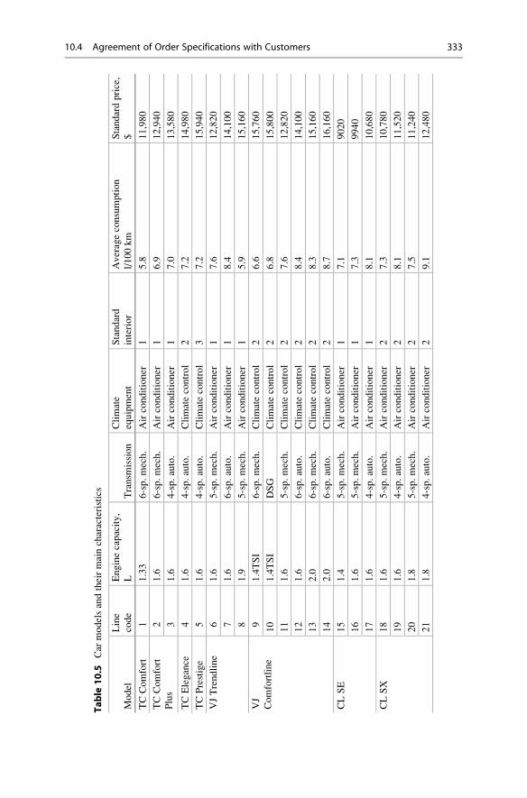
Table
10.5
Car
modelsandtheirmaincharacteristics
Model
Line
code
Enginecapacity,
LTransm
ission
Climate
equipment
Standard
interior
Averageconsumption
l/100km
Standardprice,
$
TCComfort
11.33
6-sp.mech.
Airconditioner
15.8
11,980
TCComfort
Plus
21.6
6-sp.mech.
Airconditioner
16.9
12,940
31.6
4-sp.auto.
Airconditioner
17.0
13,580
TCElegance
41.6
4-sp.auto.
Climatecontrol
27.2
14,980
TCPrestige
51.6
4-sp.auto.
Climatecontrol
37.2
15,940
VJTrendline
61.6
5-sp.mech.
Airconditioner
17.6
12,820
71.6
6-sp.auto.
Airconditioner
18.4
14,100
81.9
5-sp.mech.
Airconditioner
15.9
15,160
VJ
Comfortline
91.4TSI
6-sp.mech.
Climatecontrol
26.6
15,760
10
1.4TSI
DSG
Climatecontrol
26.8
15,800
11
1.6
5-sp.mech.
Climatecontrol
27.6
12,820
12
1.6
6-sp.auto.
Climatecontrol
28.4
14,100
13
2.0
6-sp.mech.
Climatecontrol
28.3
15,160
14
2.0
6-sp.auto.
Climatecontrol
28.7
16,160
CLSE
15
1.4
5-sp.mech.
Airconditioner
17.1
9020
16
1.6
5-sp.mech.
Airconditioner
17.3
9940
17
1.6
4-sp.auto.
Airconditioner
18.1
10,680
CLSX
18
1.6
5-sp.mech.
Airconditioner
27.3
10,780
19
1.6
4-sp.auto.
Airconditioner
28.1
11,520
20
1.8
5-sp.mech.
Airconditioner
27.5
11,240
21
1.8
4-sp.auto.
Airconditioner
29.1
12,480
10.4 Agreement of Order Specifications with Customers 333
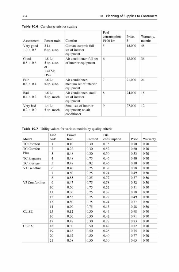
Table 10.7 Utility values for various models by quality criteria
Model
Line
code
Power
train Comfort
Fuel
consumption Price Warranty
TC Comfort 1 0.10 0.30 0.75 0.70 0.70
TC Comfort
Plus
2 0.22 0.30 0.52 0.60 0.70
3 0.48 0.30 0.50 0.53 0.70
TC Elegance 4 0.48 0.75 0.46 0.40 0.70
TC Prestige 5 0.48 0.92 0.46 0.30 0.70
VJ Trendline 6 0.40 0.25 0.38 0.58 0.50
7 0.60 0.25 0.24 0.49 0.50
8 0.85 0.25 0.72 0.37 0.50
VJ Comfortline 9 0.47 0.75 0.58 0.32 0.50
10 0.50 0.75 0.52 0.31 0.50
11 0.30 0.75 0.38 0.58 0.50
12 0.53 0.75 0.22 0.49 0.50
13 0.80 0.75 0.24 0.37 0.50
14 0.90 0.75 0.13 0.28 0.50
CL SE 15 0.12 0.30 0.44 0.98 0.70
16 0.30 0.30 0.42 0.91 0.70
17 0.48 0.30 0.28 0.83 0.70
CL SX 18 0.30 0.50 0.42 0.82 0.70
19 0.48 0.50 0.28 0.75 0.70
20 0.62 0.50 0.40 0.77 0.70
21 0.68 0.50 0.10 0.65 0.70
Table 10.6 Car characteristics scaling
Assessment Power train Comfort
Fuel
consumption
l/100 km
Price,
$
Warranty,
months
Very good
1.0 � 0.8
2 L;
6-sp. auto.
Climate control; full
set of interior
equipment
5 15,000 48
Good
0.8 � 0.6
1.8 L;
5-sp. auto.
or
1.4TSI;
DSG
Air conditioner; full set
of interior equipment
6 18,000 36
Fair
0.6 � 0.4
1.6 L;
5-sp. auto.
Air conditioner;
medium set of interior
equipment
7 21,000 24
Bad
0.4 � 0.2
1.6 L;
5-sp. mech.
Air conditioner; small
set of interior
equipment
8 24,000 18
Very bad
0.2 � 0.0
1.4 L;
5-sp. mech.
Small set of interior
equipment; no air
conditioner
9 27,000 12
334 10 Planning of Supplies to Consumers
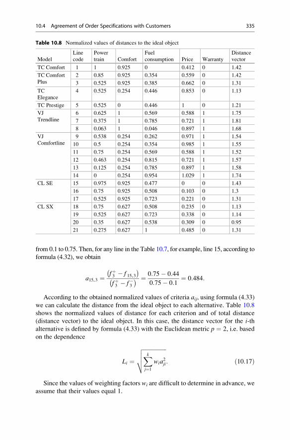
from 0.1 to 0.75. Then, for any line in the Table 10.7, for example, line 15, according to
formula (4.32), we obtain
a15,3 ¼fþ3 � f 15,3� fþ3 � f�3� ¼ 0:75� 0:44
0:75� 0:1¼ 0:484:
According to the obtained normalized values of criteria aij, using formula (4.33)
we can calculate the distance from the ideal object to each alternative. Table 10.8
shows the normalized values of distance for each criterion and of total distance
(distance vector) to the ideal object. In this case, the distance vector for the i-thalternative is defined by formula (4.33) with the Euclidean metric p ¼ 2, i.e. based
on the dependence
Li ¼ffiffiffiffiffiffiffiffiffiffiffiffiffiffiffiffiffiXkj¼1
wia2ji
vuut : ð10:17Þ
Since the values of weighting factors wi are difficult to determine in advance, we
assume that their values equal 1.
Table 10.8 Normalized values of distances to the ideal object
Model
Line
code
Power
train Comfort
Fuel
consumption Price Warranty
Distance
vector
TC Comfort 1 1 0.925 0 0.412 0 1.42
TC Comfort
Plus
2 0.85 0.925 0.354 0.559 0 1.42
3 0.525 0.925 0.385 0.662 0 1.31
TC
Elegance
4 0.525 0.254 0.446 0.853 0 1.13
TC Prestige 5 0.525 0 0.446 1 0 1.21
VJ
Trendline
6 0.625 1 0.569 0.588 1 1.75
7 0.375 1 0.785 0.721 1 1.81
8 0.063 1 0.046 0.897 1 1.68
VJ
Comfortline
9 0.538 0.254 0.262 0.971 1 1.54
10 0.5 0.254 0.354 0.985 1 1.55
11 0.75 0.254 0.569 0.588 1 1.52
12 0.463 0.254 0.815 0.721 1 1.57
13 0.125 0.254 0.785 0.897 1 1.58
14 0 0.254 0.954 1.029 1 1.74
CL SE 15 0.975 0.925 0.477 0 0 1.43
16 0.75 0.925 0.508 0.103 0 1.3
17 0.525 0.925 0.723 0.221 0 1.31
CL SX 18 0.75 0.627 0.508 0.235 0 1.13
19 0.525 0.627 0.723 0.338 0 1.14
20 0.35 0.627 0.538 0.309 0 0.95
21 0.275 0.627 1 0.485 0 1.31
10.4 Agreement of Order Specifications with Customers 335
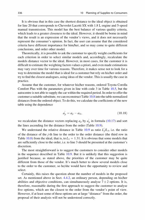
It is obvious that in this case the shortest distance to the ideal object is obtained
for line 20 that corresponds to Chevrolet Lacetti SX with 1.8 L engine and 5-speed
manual transmission. This model has the best balance of various quality criteria,
which leads to a greater closeness to the ideal. However, it should be borne in mind
that the result is an expression of the vendor’s views, and it does not necessarily
represent the consumer’s opinion. In fact, the user can assume that the considered
criteria have different importance for him/her, and so may come to quite different
conclusions, and order other model.
Theoretically, it is possible to ask the customer to specify weight coefficients for
each criterion in order to select similar models and, accordingly, recalculate the
models distance vector to the ideal. However, in most cases, for the customer it is
difficult to estimate the weighting factors values a priori, and even made estimations
may vary over time for various reasons. Therefore, it makes sense not to look for a
way to determine the model that is ideal for a customer but rely on his/her order and
try to find the closest analogues, using ideas of the vendor. This is usually the case in
practice.
Assume that the customer, for whatever his/her reasons, ordered Toyota Corolla
Comfort Plus with the parameters given in line with code 3 in Table 10.5, but the
autocentre is not able to supply the car within the required period. In order to offer the
customer a suitable substitute, we can reconstruct Table 10.8 into the table normalized
distances from the ordered object. To do this, we calculate the coefficients of the new
table using the dependence
a0ji ¼ aji � a3i; ð10:18Þ
we recalculate the distance vectors replacing aji by a0ji in formula (10.17) and sort
the lines ascending for the distance from the order (Table 10.9).
We understand the relative distance in Table 10.9 as ratio L0j/L3, i.e. the ratio
of the distance of the j-th line to the order to the order distance (the third row in
Table 10.8) from the ideal, that is, to L3 ¼ 1:31. It is obvious that some models that
are sufficiently close to the order, i.e. to line 3 should be presented at the customer’s
discretion.
The most straightforward is to suggest the customers to consider other models
in the sequence described in Table 10.9. But it is unlikely that this suggestion is
justified because, as stated above, the priorities of the customer may be quite
different from those of the vendor. It’s much better to show several models close
to the order to the customer, so he/she would have the opportunity to review and
select.
Certainly, this raises the question about the number of models in the proposed
set. As mentioned above in Sect. 4.4.2, an ordinary person, depending on his/her
abilities and objective conditions, can simultaneously analyse 7� 2 options. It is,
therefore, reasonable during the first approach to suggest the customer to analyse
five options, which are the closest to the order from the vendor’s point of view.
However, if at least some of these options are at large “distance” from the order, the
proposal of their analysis will not be understood correctly.
336 10 Planning of Supplies to Consumers
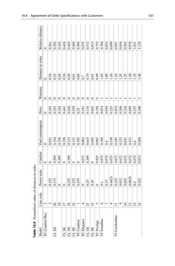
Table
10.9
Norm
alized
values
ofdistancesto
order
Model
Linecode
Power
train
Comfort
Fuel
consumption
Price
Warranty
Distance
toorder
Relativedistance
TCComfortPlus
30
00
00
00
20.325
00.031
0.103
00.34
0.261
CLSX
20
0.175
0.299
0.154
0.353
00.52
0.395
19
00.299
0.338
0.324
00.56
0.424
CLSE
17
00
0.338
0.441
00.56
0.424
CLSX
18
0.225
0.299
0.123
0.426
00.58
0.443
CLSE
16
0.225
00.123
0.559
00.61
0.469
TCComfort
10.475
00.385
0.25
00.66
0.504
TCElegance
40
0.672
0.062
0.191
00.7
0.535
CLSX
21
0.25
0.299
0.615
0.176
00.75
0.572
CLSE
15
0.45
00.092
0.662
00.81
0.615
TCPrestige
50
0.925
0.062
0.338
00.99
0.753
VJTrendline
60.1
0.075
0.185
0.074
11.03
0.784
70.15
0.075
0.4
0.059
11.09
0.833
80.4625
0.075
0.338
0.235
11.18
0.899
VJComfortline
11
0.225
0.672
0.185
0.074
11.24
0.947
90.012
0.672
0.123
0.309
11.25
0.954
10
0.025
0.672
0.031
0.324
11.25
0.952
12
0.0625
0.672
0.431
0.059
11.28
0.978
13
0.4
0.672
0.4
0.235
11.35
1.031
14
0.525
0.672
0.569
0.368
11.48
1.128
10.4 Agreement of Order Specifications with Customers 337

In the paper (Mauergauz 1989), the concept of “search radius” was introduced,
which determines the selection from the database of the objects in the vicinity of the
ordered object. The search radius means the hypersphere radius centred at the point of
order; the distance vectors of the objects, selected for consideration, are inside the
hypersphere. When negotiating with the customer, the vendor has to determine the
optimal search radius for this customerwith the use of own experience and negotiating
skills.
The search radius value can be set as the relative distance in Table 10.9multiplied
by 100 %. In this case, these relative distances are quite large, so that even when the
search radius equals 40 %, the area of selection will include only two models (lines
3 and 20). In those cases where the search area of the predetermined seraph radius
includesmanymodels, one can initially offer five of them for consideration, and then
increase this number to nine.
In this example, weighting factors wi for all i-th criteria were equated to unity.
This led to the fact that all models of Volkswagen Jetta were actually withdrawn from
consideration because their warranty period (24 months) is much less than that of the
models of other two brands (36 months). If, for example, for criterion “warranty
period” ( i ¼ 5 ) weighting factor w5 ¼ 0:5 is set, then the utility of review of
Volkswagen Jetta models will be significantly increased. In particular, VJ Trendline
model with line code 6 and relative distance 0.568 will become the closest to the
order, i.e. it will be in the ninth place and may be presented to the customer for
consideration.
The experience has shown (Lambert 1994) that the provision the opportunity for
the customer to analyse options close to the order dramatically increases the level of
service. For example, when the initial service level is 70 %, i.e. only seven orders
out of ten are fulfilled, after the customer’s considering the options of the first
selection, the service level increased to about 90 %, and after the second selection—
to nearly 97 %.
References
Lambert, D. M. (1994). Customer service strategy and management. In J. F. Robeson & W. C.
Copacino (Eds.), The logistic handbook (pp. 76–110). New York: The Free Press.
Mauergauz, Y. E. (1989). Automated design based on analogies. Chemical & Petroleum MachineBuilding, 2, 34–36 (in Russian).
Stadtler, H., & Kilger, C. (2008). Supply chain management and advanced planning. Concepts,models, software, and case studies (4th ed.). Berlin: Springer.
Vollmann, T. E., Berry, W. L., Whybark, D. C., & Jacobs, F. R. (2005). Manufacturing planningand control for supply chain management. Boston: McGraw Hill.
338 10 Planning of Supplies to Consumers
Lot Sizing 11
11.1 Classification of Lot-Sizing Problems
The chapters above widely use the notion of a batch (lot) as a set of same-type
discrete products or as a certain bulk of some material. This interpretation is based
on some definitions of the batch adopted in MRP II systems. These definitions are
described below:
• Quantity planned for production under a plan of sales and operations, master
production schedule, or material requirements schedule;
• Quantity specified in a shop floor schedule and to be processed on a single
machine without any setups (production batch);
• Quantity specified in a shop floor schedule for joint shipment (shipment batch);
• Order size in the supply chain;
• Set of identical products subject to a special batch-based inventory control;
• Quantity of products corresponding to the same quantity specified in a respective
order (lot for lot).
11.1.1 Lot Properties and Main Problems
As mentioned in Sachko (2008), lot sizes greatly depend on three factors, i.e. eco-
nomic, process, and social. The classic supply management model (Economic Order
Quantity—EOQ) described in Sect. 2.1.1 demonstrates a purely economic method of
lot sizing. Purely process approach to lot sizing provides for the use of formula (3.27)
described in Sect. 3.4. And finally, social studies (Sachko 2008) demonstrate that a
worker needs to produce 100 pieces to fully master to the process. However, once
1000 identical pieces have been processed, a worker will start experience ever-rising
fatigue due to monotony of labour.
Sizes and, consequently, quantity of product lots that are in production con-
stantly change as far as they are being processed. As a rule, the so-called release lot
# Springer International Publishing Switzerland 2016
Y. Mauergauz, Advanced Planning and Scheduling in Manufacturing and SupplyChains, DOI 10.1007/978-3-319-27523-9_11
339
(start of production process) has the greatest size while the “output” lot containing
finished products will be the smallest. Technically, the production process may
feature intermediate lot sizes; however, this makes production management quite
challenging.
In fact, the production planning process from the master plan to daily/shift targets
is to determine start and end time points for different production activities/jobs done
to product lots. The size of each lot can be specified either at a higher level of
planning before actual production planning starts or directly at the current stage of
shop floor scheduling. Here, we will consider lot-sizing process as an activity
preceding actual planning. The other approach that is more challenging will be
described below in Chaps. 13–15.
Production lots may have some peculiar features that affect the planning process
(Tanaev et al. 1998). First of all, lots are described by the method of processing
termination. In the first case, processing is finished individually where each discrete
product leaves processing site right after its termination. Here, the transfer lot size
will be 1. In the other extreme case, the lot leaves the processing site on the whole;
so, the transfer lot is equal to the production lot.
Naturally, there are intermediate cases where a production place splits into some
transfer lots under a processing job. This is the case, for example, for the most pro-
cessing time jobwhere the startup lot is divided into a number of output lots. Another
example of splitting the initial lot into sub-lots is the so-called parallel-successive
processing (Sachko 2008).
Another peculiar property of a lot is the processing procedure for individual lot
items. Technically, there are two options as follows: (a) each lot item is processed
individually one after another and (b) the whole lot is processed at a time (furnaces,
baths, etc.).
And finally, it is important whether there is a maximum lot size limit. Such limit
is often caused by a limited size of a pallet, container, buffer, transitional vessel, etc.
The optimal lot sizing can be based on either single-parameter ormultiple-parameter
approach.The aboveEOQmodel is a classic example of the single-parameter approach.
Section 4.2.2 describes lot sizing using two parameters, and three-parameter approach
is described in Sect. 4.4.2. Anyway, most lot-sizing problems use the single-parameter
optimization approach.
The existing classification of single-parameter optimization problems is described,
for example, in Jans and Degraeve (2008). The lot-sizing problem itself is generally
reduced on one of the following options:
• One product and no capacity limits:
– constant demand and constant price;
– constant demand and variable price that depends on the lot size;
– variable demand.
• Multiple products manufactured on a single machine; capacity limits; and finite
planning horizon including multiple time buckets:
– multiple different products are manufactured during each time bucket (large);
340 11 Lot Sizing
– only one type of products is manufactured during a small time bucket (regard-
less of the machine load);
– only one type of product is manufactured during each (small) time bucket
with the machine load being either full or zero;
– either one single type or two different types of products can be manufactured
during each (small) time bucket.
• The lot of finished products (or their components) is assembled from multiple
products of different types.
• Multiple products of different types are ordered simultaneously.
11.1.2 Lot-Sizing Problems with No Capacity Limits
The optimality parameter used in single-product problems with a constant demand
and no capacity limits is the cost associated with lot processing and product inven-
tory holding during an indefinite time period. If the product price depends on the lot
size, the classic EOQ model gets more complicated as the cost formula needs to be
changed. In this case, the formula (2.2) of cost during a demand period is as follows:
c ¼ Dcpj þ Q
2ch þ D
Qco; ð11:1Þ
where (as before) co represents the costs associated with order performance, chrepresents the costs associated with holding of a product item (in respective mea-
suring units) during a certain time unit, D is the quantity of product consumed
during a certain time unit, and Q is the lot size. The product price Cpj is different at
each j-interval of lot size.All other cases listed in Sect. 11.1.1 describe dynamic lot-sizing problems; they
are characterized by a variable demand and finite planning horizon. The optimality
parameter used in dynamic lot-sizing problemswith a single product, variable demand,
and no capacity limits is the minimum cost associated with pre-production (setup),
production, and product inventory holding during a limited time period h:
c ¼Xht¼1
cmXt þ coδt þ chZtð Þ; ð11:2Þ
where cm represents the production cost per product unit, co represents the cost ofregular setup required to start operations during the established period, ch representsthe cost of holding per product unit during a time period, Xt stands for the product
quantity manufactured during period t, δt is a binary variable representing setup or
no setup during period t, and Zt is the product quantity in storage by the end of
period t.
11.1 Classification of Lot-Sizing Problems 341
The stock quantity at the end of period t is as follows:
Zt ¼ Zt�1 þ Xt � Dt; ð11:3Þwhere Dt is the forecasted demand during the planned period.
Product quantity during each period t that features production setups should be
less than the cumulative (total) demand for the whole planning period, i.e.:
Xt �Xht¼1
Dt � δt at δt ∈ 0:1f g: ð11:4Þ
Naturally, Xt and Zt must be non-negative.
11.1.3 Lot-Sizing Problems with Limited Capacities and LargePlanning Periods
Here, we will describe Capacitated Multi-Item Lot-Sizing Problems (CLSP). Under
such problems, the time period in question till planning horizon h includes multiple
large time buckets. The multi-item production is planned for each of such time buckets.
Let us assume that during each time bucket t the machine capacity is Pt hours, and
the part of machine capacity equalling to pi hours is used per measuring unit of
i-product item.
Similarly to the previous problem, the optimality parameter is the minimum cost
for n manufactured product items.
c ¼Xni¼1
Xht¼1
cmiXit þ coiδit þ chiZitð Þ; ð11:5Þ
where all variables and coefficients described above in Sect. 11.1.2 depend on the
type of product item i. The stock limit (formula 11.2) gets transformed into a set of
inequalities as follows:
Zit ¼ Zi, t�1 þ Xit � Dit at 1 � i � n, 1 � t � h; ð11:6Þand the product quantity limit for a period (formula 11.3) transforms into the system
of inequalities as follows:
Xit � M � δit at δit ∈ 0; 1f g: ð11:7ÞIn expression (11.7) “the big number M” is generally determined as follows:
342 11 Lot Sizing
M ¼ min Pt=pi,Xht¼1
Dit
!at 1 � i � n: ð11:8Þ
In addition to constraints (11.6) and (11.7) that are similar to constraints listed in
Sect. 11.1.2, we get another inequality describing capacity limits:
Xni¼1
piXit � Pt: ð11:9Þ
11.1.4 Lot-Sizing Problems with Limited Capacities and SmallPlanning Periods
Here, we will describe Continuous Setup Lot-Sizing Problems (CSLP). Under such
problems, time buckets that compose the whole planning period until the planning
horizon are small; therefore, each time bucket features only one setup to adjust
machine for another product item (such setup takes place at the beginning of the
time bucket). So, we have two types of setups, i.e. regular setup that takes place at
the job start during each time bucket twith the associated cost of regular productionsetup co and additional setup required to adjust production from one product item to
another with the associated cost cs. Here, the optimality parameter is the minimum
cost
c ¼Xni¼1
Xht¼1
cmiXit þ coiδit þ csiγit þ chiZitð Þ; ð11:10Þ
unlike expression (11.5), the above expression has an additional component, i.e. csiγit.Similar to δit, γit determines the fact ofmachine setup fromone product item to another
and can take on either 0 or 1.
Stock constraints (11.5) remain unchanged:
Zit ¼ Zi, t�1 þ Xit � Dit at 1 � i � n, 1 � t � h; ð11:11Þwhile the capacity limit (11.9) is replaced by a set of constraints as follows:
piXit � Pt at1 � i � n, 1 � t � h: ð11:12ÞAs under these problems, only one product item can be manufactured during one
time bucket t, we need to introduce another constraint as follows:
11.1 Classification of Lot-Sizing Problems 343
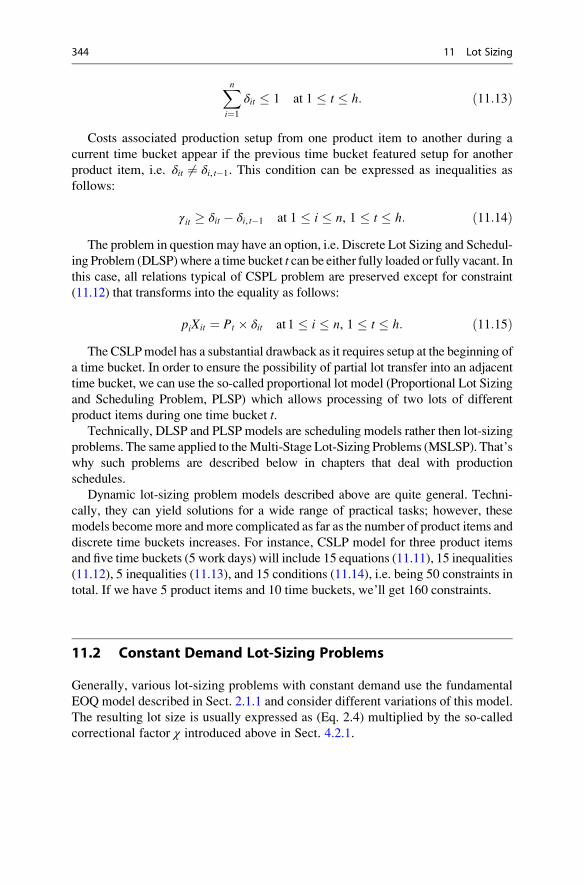
Xni¼1
δit � 1 at 1 � t � h: ð11:13Þ
Costs associated production setup from one product item to another during a
current time bucket appear if the previous time bucket featured setup for another
product item, i.e. δit 6¼ δi, t�1. This condition can be expressed as inequalities as
follows:
γit � δit � δi, t�1 at 1 � i � n, 1 � t � h: ð11:14ÞThe problem in question may have an option, i.e. Discrete Lot Sizing and Schedul-
ing Problem (DLSP)where a time bucket t can be either fully loaded or fully vacant. Inthis case, all relations typical of CSPL problem are preserved except for constraint
(11.12) that transforms into the equality as follows:
piXit ¼ Pt � δit at1 � i � n, 1 � t � h: ð11:15ÞThe CSLPmodel has a substantial drawback as it requires setup at the beginning of
a time bucket. In order to ensure the possibility of partial lot transfer into an adjacent
time bucket, we can use the so-called proportional lot model (Proportional Lot Sizing
and Scheduling Problem, PLSP) which allows processing of two lots of different
product items during one time bucket t.Technically, DLSP and PLSP models are scheduling models rather then lot-sizing
problems. The same applied to theMulti-Stage Lot-Sizing Problems (MSLSP). That’s
why such problems are described below in chapters that deal with production
schedules.
Dynamic lot-sizing problem models described above are quite general. Techni-
cally, they can yield solutions for a wide range of practical tasks; however, these
models becomemore andmore complicated as far as the number of product items and
discrete time buckets increases. For instance, CSLP model for three product items
and five time buckets (5 work days) will include 15 equations (11.11), 15 inequalities
(11.12), 5 inequalities (11.13), and 15 conditions (11.14), i.e. being 50 constraints in
total. If we have 5 product items and 10 time buckets, we’ll get 160 constraints.
11.2 Constant Demand Lot-Sizing Problems
Generally, various lot-sizing problems with constant demand use the fundamental
EOQ model described in Sect. 2.1.1 and consider different variations of this model.
The resulting lot size is usually expressed as (Eq. 2.4) multiplied by the so-called
correctional factor χ introduced above in Sect. 4.2.1.
344 11 Lot Sizing
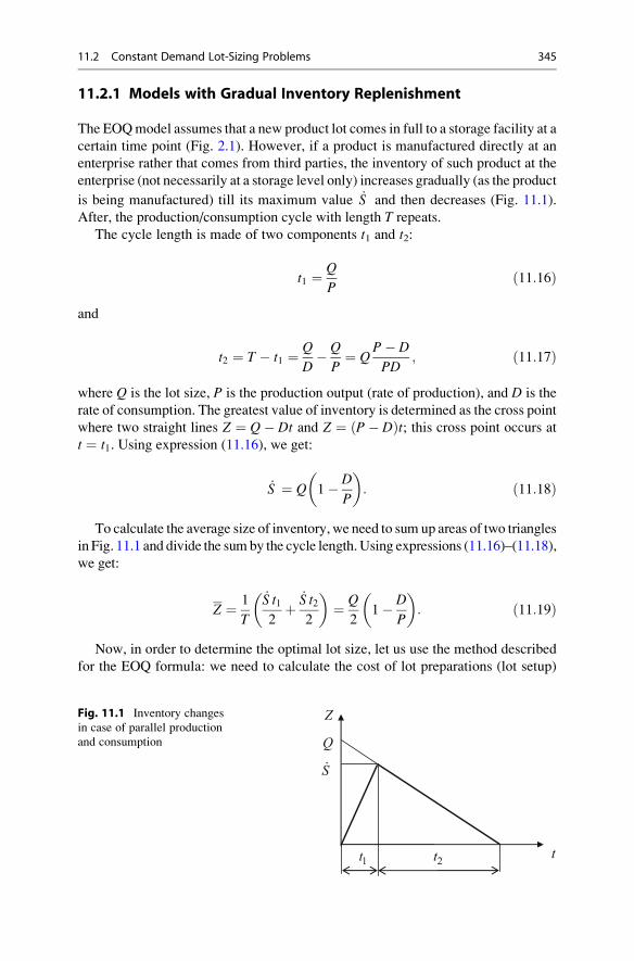
11.2.1 Models with Gradual Inventory Replenishment
The EOQmodel assumes that a new product lot comes in full to a storage facility at a
certain time point (Fig. 2.1). However, if a product is manufactured directly at an
enterprise rather that comes from third parties, the inventory of such product at the
enterprise (not necessarily at a storage level only) increases gradually (as the product
is being manufactured) till its maximum value _S and then decreases (Fig. 11.1).
After, the production/consumption cycle with length T repeats.
The cycle length is made of two components t1 and t2:
t1 ¼ Q
Pð11:16Þ
and
t2 ¼ T � t1 ¼ Q
D� Q
P¼ Q
P� D
PD; ð11:17Þ
where Q is the lot size, P is the production output (rate of production), and D is the
rate of consumption. The greatest value of inventory is determined as the cross point
where two straight lines Z ¼ Q� Dt and Z ¼ P� Dð Þt; this cross point occurs att ¼ t1. Using expression (11.16), we get:
_S ¼ Q 1� D
P
� �: ð11:18Þ
To calculate the average size of inventory, we need to sum up areas of two triangles
in Fig. 11.1 and divide the sumby the cycle length.Using expressions (11.16)–(11.18),
we get:
Z ¼ 1
T
_S t12
þ_S t22
� �¼ Q
21� D
P
� �: ð11:19Þ
Now, in order to determine the optimal lot size, let us use the method described
for the EOQ formula: we need to calculate the cost of lot preparations (lot setup)
t
Z
1t 2t
S
Q.
Fig. 11.1 Inventory changes
in case of parallel production
and consumption
11.2 Constant Demand Lot-Sizing Problems 345
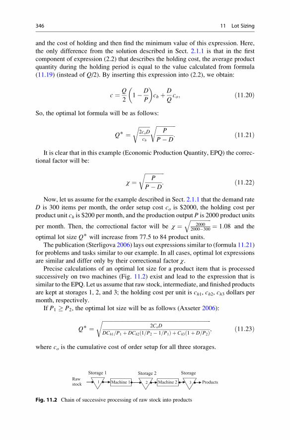
and the cost of holding and then find the minimum value of this expression. Here,
the only difference from the solution described in Sect. 2.1.1 is that in the first
component of expression (2.2) that describes the holding cost, the average product
quantity during the holding period is equal to the value calculated from formula
(11.19) (instead of Q/2). By inserting this expression into (2.2), we obtain:
c ¼ Q
21� D
P
� �ch þ D
Qco; ð11:20Þ
So, the optimal lot formula will be as follows:
Q∗ ¼ffiffiffiffiffiffiffiffi2coD
ch
r ffiffiffiffiffiffiffiffiffiffiffiffiffiffiP
P� D:
rð11:21Þ
It is clear that in this example (Economic Production Quantity, EPQ) the correc-
tional factor will be:
χ ¼ffiffiffiffiffiffiffiffiffiffiffiffiffiffiP
P� D:
rð11:22Þ
Now, let us assume for the example described in Sect. 2.1.1 that the demand rate
D is 300 items per month, the order setup cost co is $2000, the holding cost per
product unit ch is $200 per month, and the production output P is 2000 product units
per month. Then, the correctional factor will be χ ¼ffiffiffiffiffiffiffiffiffiffiffiffiffiffiffi
20002000�300
q¼ 1:08 and the
optimal lot size Q∗ will increase from 77.5 to 84 product units.
The publication (Sterligova 2006) lays out expressions similar to (formula 11.21)
for problems and tasks similar to our example. In all cases, optimal lot expressions
are similar and differ only by their correctional factor χ.Precise calculations of an optimal lot size for a product item that is processed
successively on two machines (Fig. 11.2) exist and lead to the expression that is
similar to the EPQ. Let us assume that raw stock, intermediate, and finished products
are kept at storages 1, 2, and 3; the holding cost per unit is ch1, ch2, ch3 dollars permonth, respectively.
If P1 � P2, the optimal lot size will be as follows (Axseter 2006):
Q∗ ¼ffiffiffiffiffiffiffiffiffiffiffiffiffiffiffiffiffiffiffiffiffiffiffiffiffiffiffiffiffiffiffiffiffiffiffiffiffiffiffiffiffiffiffiffiffiffiffiffiffiffiffiffiffiffiffiffiffiffiffiffiffiffiffiffiffiffiffiffiffiffiffiffiffiffiffiffiffiffiffi
2CoD
DCh1=P1 þ DCh2 1=P2 � 1=P1ð Þ þ Ch3 1þ D=P2ð Þ
r; ð11:23Þ
where co is the cumulative cost of order setup for all three storages.
Storage 1
Machine 1 Machine 2 Products
Storage 2 Storage
2 31Raw stock
Fig. 11.2 Chain of successive processing of raw stock into products
346 11 Lot Sizing
11.2.2 Model Applicable to the Machinery Industry If No CostInformation Is Available
As in the machinery industry pieces and assembly units are usually quite labour and
materials-intensive, their optimal lot sizes are determined by their processing time
and the cost of production in progress. Such problem is described in detail in Sect.
4.2.2 where we derived expression (4.33) for the optimal lot size:
Q*i ¼ A
ffiffiffiffiffiffiffiffisiDi
ci
rmeasuringunits;
where si stands for the setup time in hours, ci is the cost ofmeasuring unit,Di stands for
the demand rate in measuring units per month, and A is an undetermined dimensional
constant.
In practice, the use of formula (4.22) is quite problematic as it includes the cost of
each product item which is not always known at the time of planning. Based on
empirical evidence contained in (Guidelines of the USSR Research Institute for
Machinery, 1970), the publication (Mauergauz 2007) proposes the following for-
mula for the cost of i-item of machinery production:
ci ¼ a1 KpiniM2=3i þ biMi
� �; ð11:24Þ
where Mi stands for the unit weight in kg, ni represents the number of process jobs
done to such unit, Kpi is the production complexity factor, bi is the coefficient thatdepends on the type of materials used for production, and a1 is a certain dimen-
sional constant.
The first component of expression (11.24) represents the treatment cost while the
other component stands for the cost of materials. Treatment cost depends on the
weight of a unit to the power 2/3 as, on average, the surface area of a unit depends
on the weight to this power and processing time substantially depends exactly on
such surface area.
Besides, in this publication, (Mauergauz 2007) also assumes that if precise setup
time is not known, we can express it as follows:
si ¼ a2Ksini; ð11:25Þwhere Ksi stands for the setup complexity factor and a2 is a constant.
By inserting formulas (11.24) and (11.25) into Eq. (4.22) and taking account
undetermined constant A that can include a1 and a2, we get:
Q*i ¼ A
ffiffiffiffiffiffiffiffiffiffiffiffiffiffiffiffiffiffiffiffiffiffiffiffiffiffiffiffiffiffiffiffiffiKsiniDi
KpiniM2=3i þ biM
s: ð11:26Þ
11.2 Constant Demand Lot-Sizing Problems 347
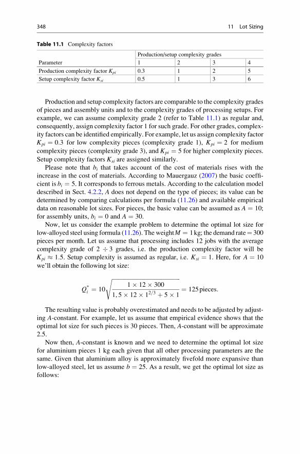
Production and setup complexity factors are comparable to the complexity grades
of pieces and assembly units and to the complexity grades of processing setups. For
example, we can assume complexity grade 2 (refer to Table 11.1) as regular and,
consequently, assign complexity factor 1 for such grade. For other grades, complex-
ity factors can be identified empirically. For example, let us assign complexity factor
Kpi ¼ 0:3 for low complexity pieces (complexity grade 1), Kpi ¼ 2 for medium
complexity pieces (complexity grade 3), and Kpi ¼ 5 for higher complexity pieces.
Setup complexity factors Ksi are assigned similarly.
Please note that bi that takes account of the cost of materials rises with the
increase in the cost of materials. According to Mauergauz (2007) the basic coeffi-
cient is bi ¼ 5. It corresponds to ferrous metals. According to the calculation model
described in Sect. 4.2.2, A does not depend on the type of pieces; its value can be
determined by comparing calculations per formula (11.26) and available empirical
data on reasonable lot sizes. For pieces, the basic value can be assumed as A ¼ 10;
for assembly units, bi ¼ 0 and A ¼ 30.
Now, let us consider the example problem to determine the optimal lot size for
low-alloyed steel using formula (11.26). TheweightM ¼ 1kg; the demand rate¼ 300
pieces per month. Let us assume that processing includes 12 jobs with the average
complexity grade of 2 � 3 grades, i.e. the production complexity factor will be
Kpi � 1:5. Setup complexity is assumed as regular, i.e. Ksi ¼ 1. Here, for A ¼ 10
we’ll obtain the following lot size:
Q*i ¼ 10
ffiffiffiffiffiffiffiffiffiffiffiffiffiffiffiffiffiffiffiffiffiffiffiffiffiffiffiffiffiffiffiffiffiffiffiffiffiffiffiffiffiffiffiffiffiffiffiffi1� 12� 300
1, 5� 12� 12=3 þ 5� 1
s¼ 125pieces:
The resulting value is probably overestimated and needs to be adjusted by adjust-
ing A-constant. For example, let us assume that empirical evidence shows that the
optimal lot size for such pieces is 30 pieces. Then, A-constant will be approximate
2.5.
Now then, A-constant is known and we need to determine the optimal lot size
for aluminium pieces 1 kg each given that all other processing parameters are the
same. Given that aluminium alloy is approximately fivefold more expansive than
low-alloyed steel, let us assume b ¼ 25. As a result, we get the optimal lot size as
follows:
Table 11.1 Complexity factors
Parameter
Production/setup complexity grades
1 2 3 4
Production complexity factor Kpi 0.3 1 2 5
Setup complexity factor Ksi 0.5 1 3 6
348 11 Lot Sizing
Q*i ¼ 2:5
ffiffiffiffiffiffiffiffiffiffiffiffiffiffiffiffiffiffiffiffiffiffiffiffiffiffiffiffiffiffiffiffiffiffiffiffiffiffiffiffiffiffiffiffiffiffiffiffiffiffi1� 12� 300
1, 5� 12� 12=3 þ 25� 1
s¼ 22pieces:
11.2.3 Three-Parameter Models for Machinery Industry
Now let us consider the problem which, in addition to setup time and cost of produc-
tion in progress described in Sect. 4.2.2, uses the parameter of time required to
process a lot. The solution to a similar multi-parameter problem is described above
in Sect. 4.4.2 where we considered different options based on a two-parameter
lot-sizing problem (refer to Sect. 4.2.2) and a minimum waiting time problem
(refer to Sect. 3.4.1). Here, we will attempt to determine a uniform relation between
the optimal lot size and three parameters. For this purpose, let us use the relation
(4.22) in the following form (4.13):
Q*i ¼ χ i
ffiffiffiffiffiffiffisiDi
ci
r;
where χ i stands for a correctional factor. The cost of production in progress ci representsdirect production costs that are equal to the sum of treatment costs and materials costs.
That’s why the formula Qi can be expressed as follows:
Q*i ¼ χ i
ffiffiffiffiffiffiffiffiffiffiffiffiffiffisiDi
τi þ biM
r; ð11:27Þ
where τi is the total treatment cost of processing per piece of i-type, bi stands for theratio between the price per 1 kg of materials to the cost of 1 labour hour, and M is
the weight of a piece.
Now, let us determine the correctional factor in formula (11.27) using available
empirical data on the relations between optimal lot sizes and machinery loads. For
this purpose, let us use Table 11.2 that has been widely used in the USSR machinery
industry.
As we can see, we can use Table 11.2 to determine the time period (cycle) of
starting the processing of the next lot based on two parameters as follows: machine
load and setup time for a machine. The parameters are determined based on the
main operation that actually depends on the design of a piece, i.e. a turning job for
rotary body pieces, a milling job for box-type piece, etc.
According to Table 11.2, standard startup periods are calculated by dividing or
multiplying the number m of work days in a month by an integer. This ensures an
even load during a month or, in case of less frequent startups, during a quarter or
6-month period. Table 11.2 is developed for those pieces whose cost of materials is
substantially lower than the cost of processing; therefore, the cost of materials has
no direct effect on lot startup standards.
11.2 Constant Demand Lot-Sizing Problems 349
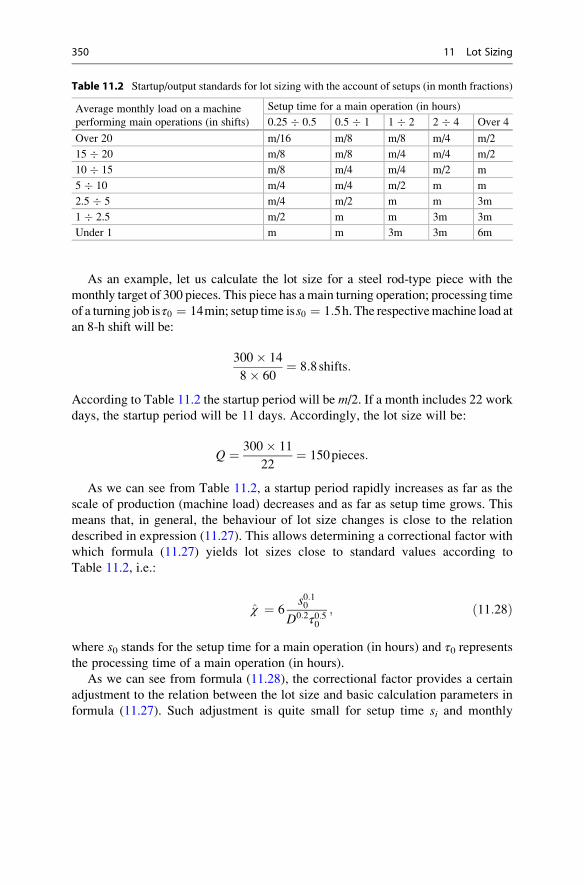
As an example, let us calculate the lot size for a steel rod-type piece with the
monthly target of 300 pieces. This piece has amain turning operation; processing time
of a turning job isτ0 ¼ 14min; setup time iss0 ¼ 1:5h. The respectivemachine load at
an 8-h shift will be:
300� 14
8� 60¼ 8:8shifts:
According to Table 11.2 the startup period will be m/2. If a month includes 22 work
days, the startup period will be 11 days. Accordingly, the lot size will be:
Q ¼ 300� 11
22¼ 150pieces:
As we can see from Table 11.2, a startup period rapidly increases as far as the
scale of production (machine load) decreases and as far as setup time grows. This
means that, in general, the behaviour of lot size changes is close to the relation
described in expression (11.27). This allows determining a correctional factor with
which formula (11.27) yields lot sizes close to standard values according to
Table 11.2, i.e.:
χ ¼ 6s0:10
D0:2τ0:50
; ð11:28Þ
where s0 stands for the setup time for a main operation (in hours) and τ0 representsthe processing time of a main operation (in hours).
As we can see from formula (11.28), the correctional factor provides a certain
adjustment to the relation between the lot size and basic calculation parameters in
formula (11.27). Such adjustment is quite small for setup time si and monthly
Table 11.2 Startup/output standards for lot sizing with the account of setups (in month fractions)
Average monthly load on a machine
performing main operations (in shifts)
Setup time for a main operation (in hours)
0.25 � 0.5 0.5 � 1 1 � 2 2 � 4 Over 4
Over 20 m/16 m/8 m/8 m/4 m/2
15 � 20 m/8 m/8 m/4 m/4 m/2
10 � 15 m/8 m/4 m/4 m/2 m
5 � 10 m/4 m/4 m/2 m m
2.5 � 5 m/4 m/2 m m 3m
1 � 2.5 m/2 m m 3m 3m
Under 1 m m 3m 3m 6m
350 11 Lot Sizing
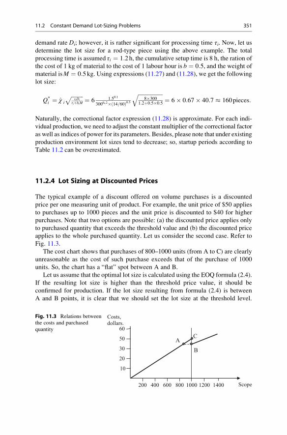
demand rate Di; however, it is rather significant for processing time τi. Now, let usdetermine the lot size for a rod-type piece using the above example. The total
processing time is assumed τi ¼ 1:2 h, the cumulative setup time is 8 h, the ration of
the cost of 1 kg of material to the cost of 1 labour hour is b ¼ 0:5, and the weight ofmaterial isM ¼ 0:5 kg. Using expressions (11.27) and (11.28), we get the followinglot size:
Q*i ¼ χ i
ffiffiffiffiffiffiffiffiffisiDi
τiþbiM
p ¼ 6 1:50:1
3000,2� 14=60ð Þ0:5ffiffiffiffiffiffiffiffiffiffiffiffiffiffiffiffiffiffi
8�3001:2þ0:5�0:5
q¼ 6� 0:67� 40:7 � 160pieces:
Naturally, the correctional factor expression (11.28) is approximate. For each indi-
vidual production, we need to adjust the constant multiplier of the correctional factor
as well as indices of power for its parameters. Besides, please note that under existing
production environment lot sizes tend to decrease; so, startup periods according to
Table 11.2 can be overestimated.
11.2.4 Lot Sizing at Discounted Prices
The typical example of a discount offered on volume purchases is a discounted
price per one measuring unit of product. For example, the unit price of $50 applies
to purchases up to 1000 pieces and the unit price is discounted to $40 for higher
purchases. Note that two options are possible: (a) the discounted price applies only
to purchased quantity that exceeds the threshold value and (b) the discounted price
applies to the whole purchased quantity. Let us consider the second case. Refer to
Fig. 11.3.
The cost chart shows that purchases of 800–1000 units (from A to C) are clearly
unreasonable as the cost of such purchase exceeds that of the purchase of 1000
units. So, the chart has a “flat” spot between A and B.
Let us assume that the optimal lot size is calculated using the EOQ formula (2.4).
If the resulting lot size is higher than the threshold price value, it should be
confirmed for production. If the lot size resulting from formula (2.4) is between
A and B points, it is clear that we should set the lot size at the threshold level.
200 400 600 800 1000 1200 Scope
Costs,dollars.
10
20
30
50
60
1400
AC
B
Fig. 11.3 Relations between
the costs and purchased
quantity
11.2 Constant Demand Lot-Sizing Problems 351
Finally, if the optimal lot size is lower than the scope of purchase at A point, we
should verify if the order cost is lower than the order cost at B point.
Let us take an example where the demand D is 2000 units per month, the cost of
one order co is $2000, and the holding cost ch is $100 per month. Using formula
(2.4), we get:
Q∗ ¼ffiffiffiffiffiffiffiffi2coD
ch
r¼
ffiffiffiffiffiffiffiffiffiffiffiffiffiffiffiffiffiffiffiffiffiffiffiffiffiffiffiffiffiffiffiffiffiffi2� 2000� 2000
100
r� 285:
According to expression (11.1) the total cost of orders during the period in question
will be as follows:
c ¼ Dcpj þ Q
2ch þ D
Qco;
where cp1 ¼ $50 per measuring unit and cp2 ¼ $40 per measuring unit. Let us com-
pare two options, i.e. an order with an optimal lot size and an order with a threshold
lot size.
In the first case, the cost of orders covering monthly demand will be:
c1 ¼ 2000� 50þ 285
2100þ 2000
2852000 ¼ 100þ 14þ 14ð Þ � 103 ¼ $128, 000
In the second case:
c2 ¼ 2000� 40þ 1000
2100þ 2000
10002000 ¼ 80þ 50þ 4ð Þ � 103 ¼ $134, 000:
As we can see, in the latter case holding costs exceed savings that can be gained
if the lot size is increased to the threshold value when a discount is offered. Other
more complex problems associated with discounted purchases are described in
detail in Lukinsky (2007).
11.3 Lot Sizing at Variable Demand and Limited PlanningHorizon
In case of variable demand, lot-sizing problems assume that the demand is known for
each discrete time bucket until the established planning horizon. Such time bucket
usually includes 1 day or 1 week; it is also assumed that the demand arises at the
beginning of the time bucket. As a rule, it is assumed that a lot comes to a storage
facility in full at the beginning of a certain time bucket; the lot lead time is ignored.
This is a classical dynamic lot-sizing problem.
It is proven that the optimal solution to such a problem has two important
properties (Axseter 2006):
352 11 Lot Sizing
(A) The product quantity in a lot is exactly equal to the cumulative demand for a
number of time buckets, i.e. for a period covered by such lot;
(B) The cost of holding for one time bucket from the whole period covered by a lot
shall not exceed the costs associated with lot shipment and delivery.
11.3.1 Exact Solution
The true and exact solution has been proposed in Wagner and Whitin (1958); today,
it is known as the Wagner–Whitin (WW) algorithm. Let us assume that demand Dt
is assigned to a number of time buckets t ¼ 1, 2, . . . h; the processing cost co perone order and holding cost ch per measuring unit during one time bucket are also
known. The solution should determine in which time bucket t every new product lot
shall be delivered and which last time bucket k it covers.Let us denote as fk,t the costs associated with lot delivery and holding till time
bucket k, starting from the time period t where the last lot has been supplied. The
minimum possible costs required to cover the demand till time bucket k will be asfollows:
f k ¼ min1�t�k
f k, t: ð11:29Þ
This means that it depends on the delivery time t.If previous costs already incurred by the time period t� 1 are known, cover
demand at this period and equal to f t�1, then costs fk,t over the next period t willdepend on the size of a lot supplied at this period. Themore bucket number k is (untilwhich a lot shall cover the demand), the more fk,t will be. It is true that:
f k, t ¼ f t�1 þ co þ ch Dtþ1 þ 2Dtþ2 þ . . .þ k � tð ÞDk½ �: ð11:30ÞAs demand Dt is covered at the beginning of time bucket co, i.e. immediately
after supply, then, holding costs are partially associated with a lot supplied in such
time bucket and intended to cover demand over next time buckets. The more distant
such next to-be-covered time bucket is from the supply time bucket t, the longer
holding period and the higher associated costs will be.
Let us consider the WW algorithm using the example described in Table 11.3.
Let us assume that management costs per one lot co ¼ $2, 000; holding costs per
product measuring unit ch ¼ $10. Let us also assume that f 0 ¼ 0.
Each line in Table 11.3 represents the biggest number of a time bucket covered
by a lot supplied in the time period t; cross cells show respective values of fk,t. Thetable starts to be filled with f1,1 ¼ co ¼ 2, 000. Such cost will occur if a lot supplied
in time bucket t ¼ 1 covers only demand over the same time bucket, i.e. k ¼ t. Thismeans that the lot immediately leaves the storage and there are no holding costs.
If the lot supplied in time bucket t ¼ 1 should also cover the next time bucket
t ¼ 2, i.e. k ¼ tþ 1, then according to formula (11.30):
11.3 Lot Sizing at Variable Demand and Limited Planning Horizon 353
Table
11.3
Dynam
iclotsize
costs
Finitehorizonforalot
Number
oftimebucket
tandrespectivedem
andDt
1/60
2/30
3/80
4/60
5/50
6/100
7/60
8/70
9/80
10/70
k¼
t2000
4000
4300
5900
6900
7900
9900
10,500
11,900
13,300
k¼
tþ1
2300
4800
4900
6400
7900
8500
10,600
11,300
12,600
k¼
tþ2
3900
6000
5900
8400
9100
9900
12,200
12,700
k¼
tþ3
5700
7500
10,200
14,300
k¼
tþ4
7700
354 11 Lot Sizing
f 2,1 ¼ f 0 þ co þ chD2 ¼ 0þ 2000þ 10� 30 ¼ 2300:
Similarly, f 3,1 ¼ 0þ2000þ10�30þ2�10�80 ¼ 3900, f 4,1 ¼ 5700, f 5,1 ¼ 7700.
For time bucket 6 holding costs are equal to 5� 10� 100 ¼ 5, 000 and exceed
co ¼ 2, 000. So, according to the property (B) described above in Sect. 11.3, it is
unreasonable to use the lot supplied in time bucket 1 to cover demand in time bucket
6 and there is no need to further fill column 1 of the table. As we can see, minimum
costs associated with lot supplies to cover demand in time period k ¼ 1 only will be
as follows: f 1 ¼ f 1,1 ¼ 2, 000.
Now, let us calculate fk,t when a new lot is supplied during time bucket t ¼ 2.
Using expression (11.30) we get:
f 2,2 ¼ f 1 þ co ¼ 2000þ 2000 ¼ 4000:
Similar to Column 1 calculations, f 3,2 ¼ 4800, f 4,2 ¼ 6000, f 5,2 ¼ 7500, and there
is no need in further calculations.
Now let us consider whether it is reasonable if a lot supplied in time bucket t ¼ 1
also covers demand in time bucket t ¼ 2, i.e. k ¼ tþ 1. For this purpose, let us use
formula (11.29) or, which is the same, compare two underlined numbers shown in
columns for time buckets 1 and 2. Both numbers apply to one and the same value
k ¼ 2, i.e. they represent the costs that are required to cover demand in time bucket
2. It turns out that if we use the lot supplied in time bucket 1, associated costs will be
$2300, while if we use another lot to cover demand in time bucket 2, associated
costs will be $4000. Accordingly:
f 2 ¼ min1�t�2
f 2, t ¼ min f 2,1; f 2,2� ¼ min 2300; 4000ð Þ ¼ 2300:
Let us proceedwithColumn3and again use formula (11.30)wheref t�1 ¼ f 2 ¼ 2, 300.
So, f 3,3 ¼ f 2 þ co ¼ 4, 300, f 4,3 ¼ 4, 900, etc. To proceed with Column 4, let us cal-
culate the following value:
f 3 ¼ min1�t�3
f 3, t ¼ min f 3,1; f 3,2; f 3,3� ¼ min 3900; 4800; 4300ð Þ ¼ 3900:
As you can see, compared values of fk,t lie on the diagonal of the table; at the last
element on the diagonal is fk,t with equal indices k ¼ t. All remaining columns
should be completed similarly.
To find the lot size solution, we should move from the last diagonal in Table 11.3.
This diagonal will yield us the solution on the minimum cumulative costs as
follows:
f 10 ¼ min 14300; 12700; 12600; 13300ð Þ ¼ 12600
This means that the last lot should be supplied in time bucket 9.
11.3 Lot Sizing at Variable Demand and Limited Planning Horizon 355
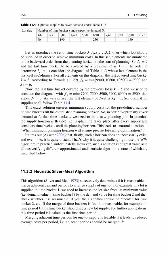
Let us introduce the set of time buckets J{J1, J2, . . . Jn}, over which lots should
be supplied in order to achieve minimum costs. In this set, elements are numbered
in the backward order from the planning horizon to the start of planning. So, J1 ¼ 9
and the last time bucket to be covered by a previous lot is k ¼ 8. In order to
determine J2 let us consider the diagonal of Table 11.3 whose last element is the
first cell in Column 8. For all elements on this diagonal, the last covered time bucket
k ¼ 8. According to formula (11.29), f 8 ¼ min 9900; 10600; 10500ð Þ ¼ 9900 and
J2 ¼ 6.
Now, the last time bucket covered by the previous lot is k ¼ 5 and we need to
consider the diagonal with f 5 ¼ min 7700; 7500; 5900; 6400; 6900ð Þ ¼ 5900 that
yields J3 ¼ 3. As we can see, the last element of J-set is J4 ¼ 1. So, optimal lot
supplies shall follow Table 11.4.
This exact solution ensures minimum supply costs for the pre-defined number
of time buckets till the established planning horizon. So, in order to optimally cover
demand at further time buckets, we need to do a new planning job. In practice,
the supply horizon is flexible, i.e. re-planning takes place after every supply and
considers time buckets until the planning horizon. This leads to a natural question—
“What minimum planning horizon will ensure precise lot-sizing optimization?”.
It turns out (Axseter 2006) that, firstly, such a horizon does not necessarily exist,
and even if so, it is quite distant. That’s why it is quite challenging to use the WW
algorithm in practice, unfortunately. However, such a solution is of great value as it
allows verifying different approximated and heuristic algorithms some of which are
described below.
11.3.2 Heuristic Silver–Meal Algorithm
This algorithm (Silver and Meal 1973) successively determines if it is reasonable to
merge adjacent demand periods to arrange supply of one lot. For example, if a lot is
supplied in time bucket 1, we need to increase the lot size from its minimum value
(i.e. demand value in time bucket 1) by the demand value for time bucket 2 and then
check whether it is reasonable. If yes, the algorithm should be repeated for time
bucket 2, etc. If the merge of time buckets is found unreasonable, for example, in
time period k, this time bucket should see a new lot supply. For further applications,
this time period k is taken as the first time period.
Merging adjacent time periods for one lot supply is feasible if it leads to reduced
average costs per period, i.e. adjacent periods should be merged if:
Table 11.4 Optimal supplies to cover demand under Table 11.3
Lot size Number of time bucket t and respective demand Dt
1/60 2/30 3/80 4/60 5/50 6/100 7/60 8/70 9/80 10/70
90 190 230 150
356 11 Lot Sizing
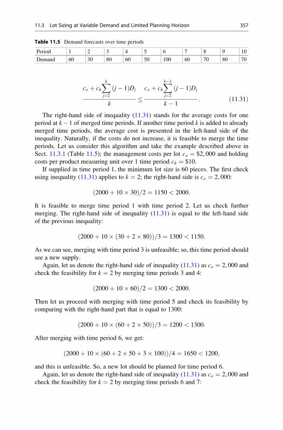
co þ chXkj¼2
j� 1ð ÞDj
k�
co þ chXk�1
j¼2
j� 1ð ÞDj
k � 1: ð11:31Þ
The right-hand side of inequality (11.31) stands for the average costs for one
period at k� 1 of merged time periods. If another time period k is added to already
merged time periods, the average cost is presented in the left-hand side of the
inequality. Naturally, if the costs do not increase, it is feasible to merge the time
periods. Let us consider this algorithm and take the example described above in
Sect. 11.3.1 (Table 11.5); the management costs per lot co ¼ $2, 000 and holding
costs per product measuring unit over 1 time period ch ¼ $10.
If supplied in time period 1, the minimum lot size is 60 pieces. The first check
using inequality (11.31) applies to k ¼ 2; the right-hand side is co ¼ 2, 000:
2000þ 10� 30ð Þ=2 ¼ 1150 < 2000:
It is feasible to merge time period 1 with time period 2. Let us check further
merging. The right-hand side of inequality (11.31) is equal to the left-hand side
of the previous inequality:
2000þ 10� 30þ 2� 80ð Þð Þ=3 ¼ 1300 < 1150:
As we can see, merging with time period 3 is unfeasible; so, this time period should
see a new supply.
Again, let us denote the right-hand side of inequality (11.31) as co ¼ 2, 000 and
check the feasibility for k ¼ 2 by merging time periods 3 and 4:
2000þ 10� 60ð Þ=2 ¼ 1300 < 2000:
Then let us proceed with merging with time period 5 and check its feasibility by
comparing with the right-hand part that is equal to 1300:
2000þ 10� 60þ 2� 50ð Þð Þ=3 ¼ 1200 < 1300:
After merging with time period 6, we get:
2000þ 10� 60þ 2� 50þ 3� 100ð Þð Þ=4 ¼ 1650 < 1200;
and this is unfeasible. So, a new lot should be planned for time period 6.
Again, let us denote the right-hand side of inequality (11.31) as co ¼ 2, 000 and
check the feasibility for k ¼ 2 by merging time periods 6 and 7:
Table 11.5 Demand forecasts over time periods
Period 1 2 3 4 5 6 7 8 9 10
Demand 60 30 80 60 50 100 60 70 80 70
11.3 Lot Sizing at Variable Demand and Limited Planning Horizon 357
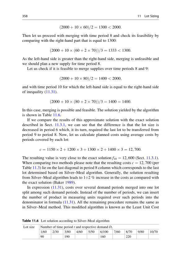
2000þ 10� 60ð Þ=2 ¼ 1300 < 2000:
Then let us proceed with merging with time period 8 and check its feasibility by
comparing with the right-hand part that is equal to 1300:
2000þ 10� 60þ 2� 70ð Þð Þ=3 ¼ 1333 < 1300:
As the left-hand side is greater than the right-hand side, merging is unfeasible and
we should plan a new supply for time period 8.
Let us check if it is feasible to merge supplies over time periods 8 and 9:
2000þ 10� 80ð Þ=2 ¼ 1400 < 2000;
and with time period 10 for which the left-hand side is equal to the right-hand side
of inequality (11.31).
2000þ 10� 80þ 2� 70ð Þð Þ=3 ¼ 1400 ¼ 1400:
In this case, merging is possible and feasible. The solution yielded by the algorithm
is shown in Table 11.6.
If we compare the results of this approximate solution with the exact solution
described in Sect. 11.3.1, we can see that the difference is that the lot size is
decreased in period 6 which, it its turn, required the last lot to be transferred from
period 9 to period 8. Now, let us calculate planned costs using average costs by
periods covered by each lot:
c ¼ 1150� 2þ 1200� 3þ 1300� 2þ 1400� 3 ¼ 12, 700:
The resulting value is very close to the exact solution f10 ¼ 12, 600 (Sect. 11.3.1).
When comparing two methods please note that the resulting costs c ¼ 12, 700 (per
Table 11.3) lie on the last diagonal in period 8 column which corresponds to the last
lot determined based on Silver–Meal algorithm. Generally, the solution resulting
from Silver–Meal algorithm leads to 1�2 % increase in the costs as compared with
the exact solution (Baker 1989).
In expression (11.31), costs over several demand periods merged into one lot
split among such demand periods. Instead of the number of periods, we can insert
the number of product in measuring units required over such periods into the
denominator in formula (11.31). All the remaining procedure remains the same as
in Silver–Meal method. This modified algorithm is known as the Least Unit Cost
Table 11.6 Lot solution according to Silver–Meal algorithm
Lot size Number of time period t and respective demand Dt
1/60 2/30 3/80 4/60 5/50 6/100 7/60 8/70 9/80 10/70
90 190 160 220
358 11 Lot Sizing
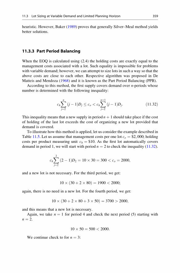
heuristic. However, Baker (1989) proves that generally Silver–Meal method yields
better solutions.
11.3.3 Part Period Balancing
When the EOQ is calculated using (2.4) the holding costs are exactly equal to the
management costs associated with a lot. Such equality is impossible for problems
with variable demand; however, we can attempt to size lots in such a way so that the
above costs are close to each other. Respective algorithm was proposed in De
Matteis and Mendoza (1968) and it is known as the Part Period Balancing (PPB).
According to this method, the first supply covers demand over n-periods whosenumber is determined with the following inequality:
chXnj¼2
j� 1ð ÞDj � co < chXnþ1
j¼2
j� 1ð ÞDj: ð11:32Þ
This inequality means that a new supply in period nþ 1 should take place if the cost
of holding of the last lot exceeds the cost of organizing a new lot provided that
demand is covered.
To illustrate how this method is applied, let us consider the example described in
Table 11.5. Let us assume that management costs per one lot co ¼ $2, 000; holding
costs per product measuring unit ch ¼ $10. As the first lot automatically covers
demand in period 1, we will start with period n ¼ 2 to check the inequality (11.32).
chX2j¼2
2� 1ð ÞD2 ¼ 10� 30 ¼ 300 < co ¼ 2000;
and a new lot is not necessary. For the third period, we get:
10� 30þ 2� 80ð Þ ¼ 1900 < 2000;
again, there is no need in a new lot. For the fourth period, we get:
10� 30þ 2� 80þ 3� 50ð Þ ¼ 3700 > 2000;
and this means that a new lot is necessary.
Again, we take n ¼ 1 for period 4 and check the next period (5) starting with
n ¼ 2.
10� 50 ¼ 500 < 2000:
We continue check to for n ¼ 3:
11.3 Lot Sizing at Variable Demand and Limited Planning Horizon 359
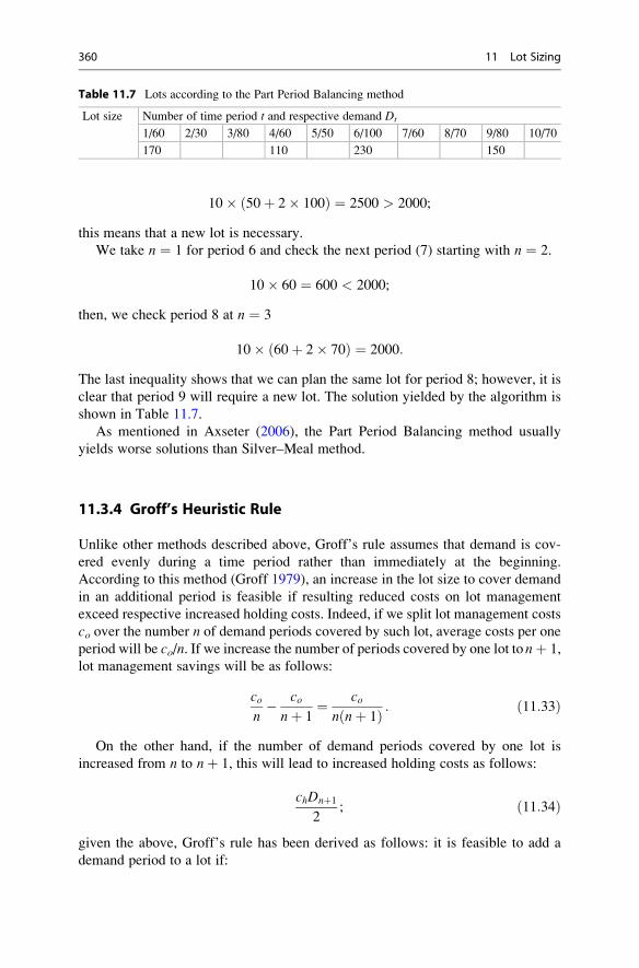
10� 50þ 2� 100ð Þ ¼ 2500 > 2000;
this means that a new lot is necessary.
We take n ¼ 1 for period 6 and check the next period (7) starting with n ¼ 2.
10� 60 ¼ 600 < 2000;
then, we check period 8 at n ¼ 3
10� 60þ 2� 70ð Þ ¼ 2000:
The last inequality shows that we can plan the same lot for period 8; however, it is
clear that period 9 will require a new lot. The solution yielded by the algorithm is
shown in Table 11.7.
As mentioned in Axseter (2006), the Part Period Balancing method usually
yields worse solutions than Silver–Meal method.
11.3.4 Groff’s Heuristic Rule
Unlike other methods described above, Groff’s rule assumes that demand is cov-
ered evenly during a time period rather than immediately at the beginning.
According to this method (Groff 1979), an increase in the lot size to cover demand
in an additional period is feasible if resulting reduced costs on lot management
exceed respective increased holding costs. Indeed, if we split lot management costs
co over the number n of demand periods covered by such lot, average costs per one
period will be co/n. If we increase the number of periods covered by one lot tonþ 1,
lot management savings will be as follows:
con� conþ 1
¼ con nþ 1ð Þ : ð11:33Þ
On the other hand, if the number of demand periods covered by one lot is
increased from n to nþ 1, this will lead to increased holding costs as follows:
chDnþ1
2; ð11:34Þ
given the above, Groff’s rule has been derived as follows: it is feasible to add a
demand period to a lot if:
Table 11.7 Lots according to the Part Period Balancing method
Lot size Number of time period t and respective demand Dt
1/60 2/30 3/80 4/60 5/50 6/100 7/60 8/70 9/80 10/70
170 110 230 150
360 11 Lot Sizing
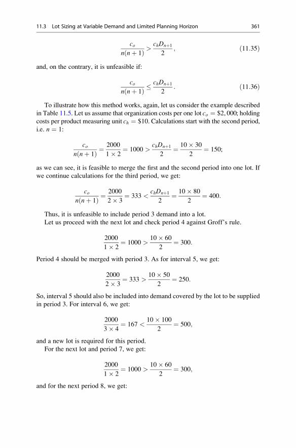
con nþ 1ð Þ >
chDnþ1
2; ð11:35Þ
and, on the contrary, it is unfeasible if:
con nþ 1ð Þ �
chDnþ1
2: ð11:36Þ
To illustrate how this method works, again, let us consider the example described
in Table 11.5. Let us assume that organization costs per one lot co ¼ $2, 000; holding
costs per product measuring unit ch ¼ $10. Calculations start with the second period,
i.e. n ¼ 1:
con nþ 1ð Þ ¼
2000
1� 2¼ 1000 >
chDnþ1
2¼ 10� 30
2¼ 150;
as we can see, it is feasible to merge the first and the second period into one lot. If
we continue calculations for the third period, we get:
con nþ 1ð Þ ¼
2000
2� 3¼ 333 <
chDnþ1
2¼ 10� 80
2¼ 400:
Thus, it is unfeasible to include period 3 demand into a lot.
Let us proceed with the next lot and check period 4 against Groff’s rule.
2000
1� 2¼ 1000 >
10� 60
2¼ 300:
Period 4 should be merged with period 3. As for interval 5, we get:
2000
2� 3¼ 333 >
10� 50
2¼ 250:
So, interval 5 should also be included into demand covered by the lot to be supplied
in period 3. For interval 6, we get:
2000
3� 4¼ 167 <
10� 100
2¼ 500;
and a new lot is required for this period.
For the next lot and period 7, we get:
2000
1� 2¼ 1000 >
10� 60
2¼ 300;
and for the next period 8, we get:
11.3 Lot Sizing at Variable Demand and Limited Planning Horizon 361
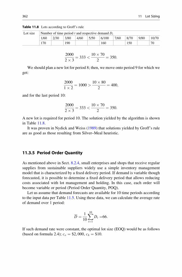
2000
2� 3¼ 333 <
10� 70
2¼ 350:
We should plan a new lot for period 8; then, we move onto period 9 for which we
get:
2000
1� 2¼ 1000 >
10� 80
2¼ 400;
and for the last period 10:
2000
2� 3¼ 333 <
10� 70
2¼ 350:
A new lot is required for period 10. The solution yielded by the algorithm is shown
in Table 11.8.
It was proven in Nydick and Weiss (1989) that solutions yielded by Groff’s rule
are as good as those resulting from Silver–Meal heuristic.
11.3.5 Period Order Quantity
As mentioned above in Sect. 8.2.4, small enterprises and shops that receive regular
supplies from sustainable suppliers widely use a simple inventory management
model that is characterized by a fixed delivery period. If demand is variable though
forecasted, it is possible to determine a fixed delivery period that allows reducing
costs associated with lot management and holding. In this case, each order will
become variable or period (Period Order Quantity, POQ).
Let us assume that demand forecasts are available for 10 time periods according
to the input data per Table 11.5. Using these data, we can calculate the average rate
of demand over 1 period:
D ¼ 1
10
X10t¼1
Dt ¼66:
If such demand rate were constant, the optimal lot size (EOQ) would be as follows
(based on formula 2.4); co ¼ $2, 000, ch ¼ $10.
Table 11.8 Lots according to Groff’s rule
Lot size Number of time period t and respective demand Dt
1/60 2/30 3/80 4/60 5/50 6/100 7/60 8/70 9/80 10/70
170 190 160 150 70
362 11 Lot Sizing
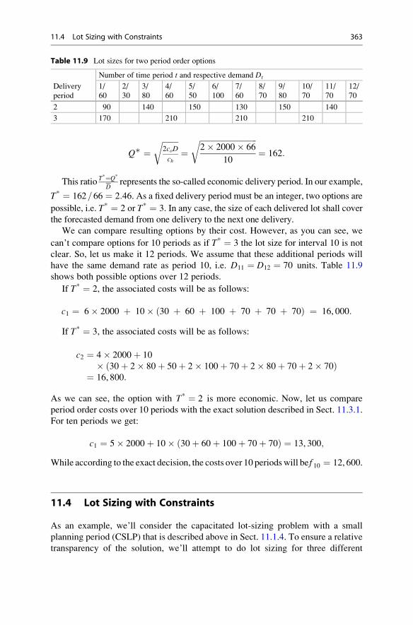
Q∗ ¼ffiffiffiffiffiffiffiffi2coD
ch
r¼
ffiffiffiffiffiffiffiffiffiffiffiffiffiffiffiffiffiffiffiffiffiffiffiffiffiffiffiffiffi2� 2000� 66
10
r¼ 162:
This ratio T*¼Q*
Drepresents the so-called economic delivery period. In our example,
T* ¼ 162=66 ¼ 2:46. As a fixed delivery period must be an integer, two options are
possible, i.e. T* ¼ 2 or T* ¼ 3. In any case, the size of each delivered lot shall cover
the forecasted demand from one delivery to the next one delivery.
We can compare resulting options by their cost. However, as you can see, we
can’t compare options for 10 periods as if T* ¼ 3 the lot size for interval 10 is not
clear. So, let us make it 12 periods. We assume that these additional periods will
have the same demand rate as period 10, i.e. D11 ¼ D12 ¼ 70 units. Table 11.9
shows both possible options over 12 periods.
If T* ¼ 2, the associated costs will be as follows:
c1 ¼ 6� 2000 þ 10� 30 þ 60 þ 100 þ 70 þ 70 þ 70ð Þ ¼ 16, 000:
If T* ¼ 3, the associated costs will be as follows:
c2 ¼ 4� 2000þ 10
� 30þ 2� 80þ 50þ 2� 100þ 70þ 2� 80þ 70þ 2� 70ð Þ¼ 16, 800:
As we can see, the option with T* ¼ 2 is more economic. Now, let us compare
period order costs over 10 periods with the exact solution described in Sect. 11.3.1.
For ten periods we get:
c1 ¼ 5� 2000þ 10� 30þ 60þ 100þ 70þ 70ð Þ ¼ 13, 300;
While according to the exact decision, the costs over 10 periodswill be f 10 ¼ 12, 600.
11.4 Lot Sizing with Constraints
As an example, we’ll consider the capacitated lot-sizing problem with a small
planning period (CSLP) that is described above in Sect. 11.1.4. To ensure a relative
transparency of the solution, we’ll attempt to do lot sizing for three different
Table 11.9 Lot sizes for two period order options
Delivery
period
Number of time period t and respective demand Dt
1/
60
2/
30
3/
80
4/
60
5/
50
6/
100
7/
60
8/
70
9/
80
10/
70
11/
70
12/
70
2 90 140 150 130 150 140
3 170 210 210 210
11.4 Lot Sizing with Constraints 363
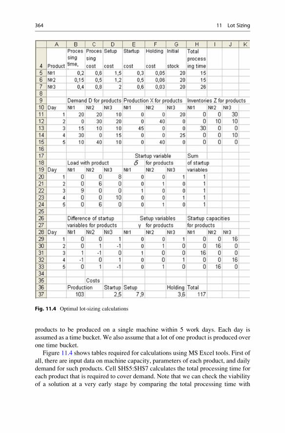
products to be produced on a single machine within 5 work days. Each day is
assumed as a time bucket. We also assume that a lot of one product is produced over
one time bucket.
Figure 11.4 shows tables required for calculations using MS Excel tools. First of
all, there are input data on machine capacity, parameters of each product, and daily
demand for such products. Cell $H$5:$H$7 calculates the total processing time for
each product that is required to cover demand. Note that we can check the viability
of a solution at a very early stage by comparing the total processing time with
Fig. 11.4 Optimal lot-sizing calculations
364 11 Lot Sizing
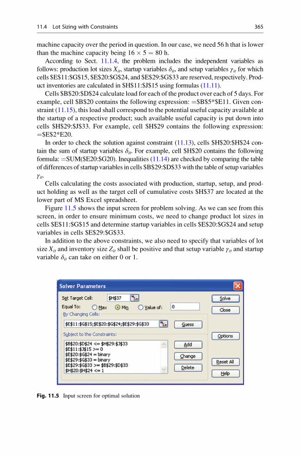
machine capacity over the period in question. In our case, we need 56 h that is lower
than the machine capacity being 16� 5 ¼ 80 h.
According to Sect. 11.1.4, the problem includes the independent variables as
follows: production lot sizes Xit, startup variables δit, and setup variables γit for whichcells $E$11:$G$15, $E$20:$G$24, and $E$29:$G$33 are reserved, respectively. Prod-
uct inventories are calculated in $H$11:$J$15 using formulas (11.11).
Cells $B$20:$D$24 calculate load for each of the product over each of 5 days. For
example, cell $B$20 contains the following expression: ¼$B$5*$E11. Given con-
straint (11.15), this load shall correspond to the potential useful capacity available at
the startup of a respective product; such available useful capacity is put down into
cells $H$29:$J$33. For example, cell $H$29 contains the following expression:
¼$E$2*E20.
In order to check the solution against constraint (11.13), cells $H$20:$H$24 con-
tain the sum of startup variables δit. For example, cell $H$20 contains the following
formula:¼SUM($E20:$G20). Inequalities (11.14) are checked by comparing the table
of differences of startup variables in cells $B$29:$D$33with the table of setup variables
γit.Cells calculating the costs associated with production, startup, setup, and prod-
uct holding as well as the target cell of cumulative costs $H$37 are located at the
lower part of MS Excel spreadsheet.
Figure 11.5 shows the input screen for problem solving. As we can see from this
screen, in order to ensure minimum costs, we need to change product lot sizes in
cells $E$11:$G$15 and determine startup variables in cells $E$20:$G$24 and setup
variables in cells $E$29:$G$33.
In addition to the above constraints, we also need to specify that variables of lot
size Xit and inventory size Zit shall be positive and that setup variable γit and startupvariable δit can take on either 0 or 1.
Fig. 11.5 Input screen for optimal solution
11.4 Lot Sizing with Constraints 365
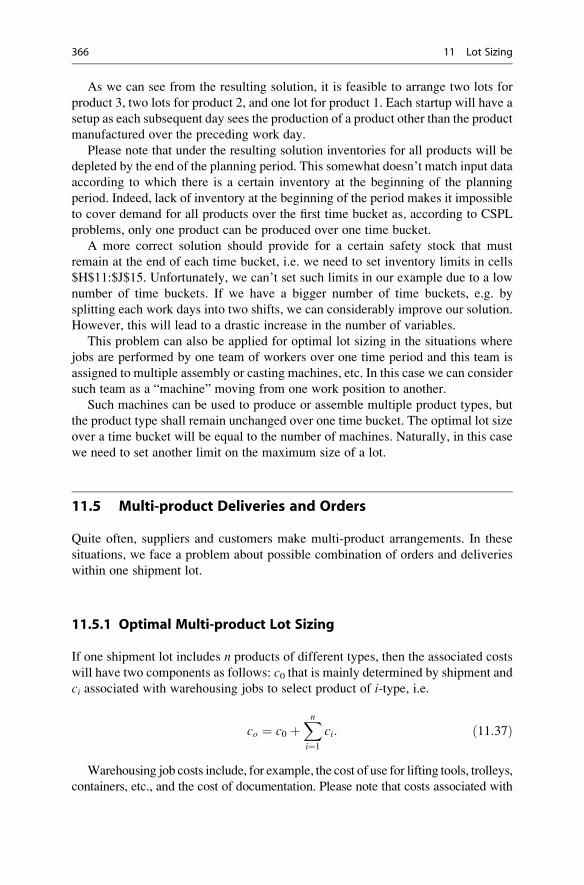
As we can see from the resulting solution, it is feasible to arrange two lots for
product 3, two lots for product 2, and one lot for product 1. Each startup will have a
setup as each subsequent day sees the production of a product other than the product
manufactured over the preceding work day.
Please note that under the resulting solution inventories for all products will be
depleted by the end of the planning period. This somewhat doesn’t match input data
according to which there is a certain inventory at the beginning of the planning
period. Indeed, lack of inventory at the beginning of the period makes it impossible
to cover demand for all products over the first time bucket as, according to CSPL
problems, only one product can be produced over one time bucket.
A more correct solution should provide for a certain safety stock that must
remain at the end of each time bucket, i.e. we need to set inventory limits in cells
$H$11:$J$15. Unfortunately, we can’t set such limits in our example due to a low
number of time buckets. If we have a bigger number of time buckets, e.g. by
splitting each work days into two shifts, we can considerably improve our solution.
However, this will lead to a drastic increase in the number of variables.
This problem can also be applied for optimal lot sizing in the situations where
jobs are performed by one team of workers over one time period and this team is
assigned to multiple assembly or casting machines, etc. In this case we can consider
such team as a “machine” moving from one work position to another.
Such machines can be used to produce or assemble multiple product types, but
the product type shall remain unchanged over one time bucket. The optimal lot size
over a time bucket will be equal to the number of machines. Naturally, in this case
we need to set another limit on the maximum size of a lot.
11.5 Multi-product Deliveries and Orders
Quite often, suppliers and customers make multi-product arrangements. In these
situations, we face a problem about possible combination of orders and deliveries
within one shipment lot.
11.5.1 Optimal Multi-product Lot Sizing
If one shipment lot includes n products of different types, then the associated costs
will have two components as follows: c0 that is mainly determined by shipment and
ci associated with warehousing jobs to select product of i-type, i.e.
co ¼ c0 þXni¼1
ci: ð11:37Þ
Warehousing job costs include, for example, the cost of use for lifting tools, trolleys,
containers, etc., and the cost of documentation. Please note that costs associated with
366 11 Lot Sizing
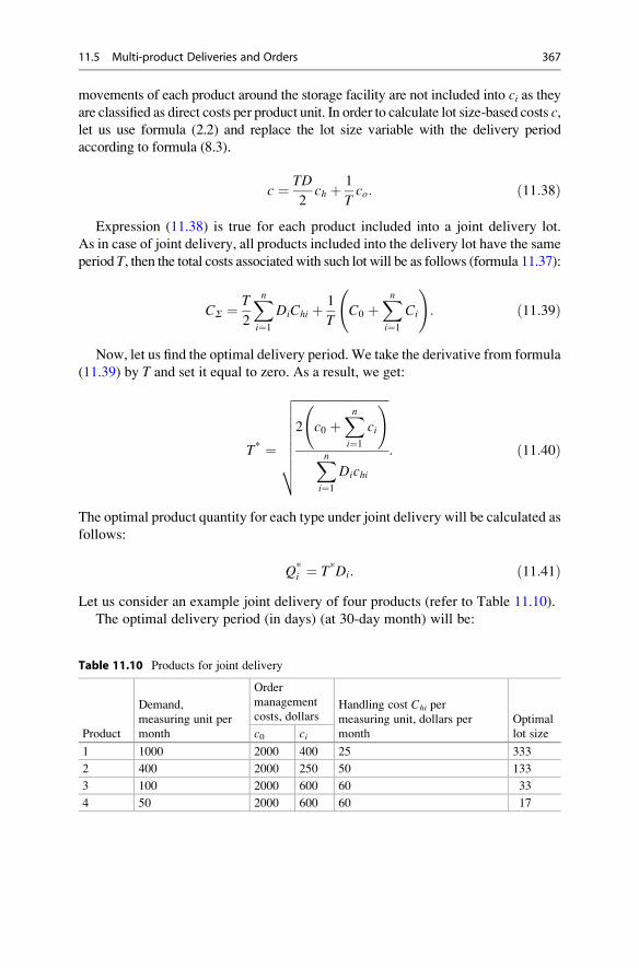
movements of each product around the storage facility are not included into ci as theyare classified as direct costs per product unit. In order to calculate lot size-based costs c,let us use formula (2.2) and replace the lot size variable with the delivery period
according to formula (8.3).
c ¼ TD
2ch þ 1
Tco: ð11:38Þ
Expression (11.38) is true for each product included into a joint delivery lot.
As in case of joint delivery, all products included into the delivery lot have the same
period T, then the total costs associated with such lot will be as follows (formula 11.37):
CΣ ¼ T
2
Xni¼1
DiChi þ 1
TC0 þ
Xni¼1
Ci
!: ð11:39Þ
Now, let us find the optimal delivery period. We take the derivative from formula
(11.39) by T and set it equal to zero. As a result, we get:
T* ¼
ffiffiffiffiffiffiffiffiffiffiffiffiffiffiffiffiffiffiffiffiffiffiffiffiffiffiffiffiffiffiffi2 c0 þ
Xni¼1
ci
!Xni¼1
Dichi
vuuuuuuut : ð11:40Þ
The optimal product quantity for each type under joint delivery will be calculated as
follows:
Q*i ¼ T*Di: ð11:41Þ
Let us consider an example joint delivery of four products (refer to Table 11.10).
The optimal delivery period (in days) (at 30-day month) will be:
Table 11.10 Products for joint delivery
Product
Demand,
measuring unit per
month
Order
management
costs, dollarsHandling cost Chi per
measuring unit, dollars per
month
Optimal
lot sizec0 ci
1 1000 2000 400 25 333
2 400 2000 250 50 133
3 100 2000 600 60 33
4 50 2000 600 60 17
11.5 Multi-product Deliveries and Orders 367
T* ¼ 30
ffiffiffiffiffiffiffiffiffiffiffiffiffiffiffiffiffiffiffiffiffiffiffiffiffiffiffiffiffiffiffiffiffiffiffiffiffiffiffiffiffiffiffiffiffiffiffiffiffiffiffiffiffiffiffiffiffiffiffiffiffiffiffiffiffiffiffiffiffiffiffiffiffiffiffiffiffiffiffiffiffiffiffiffiffiffiffiffiffi2� 2000þ 400þ 250þ 600þ 600ð Þ
1000� 25þ 400� 50þ 100� 60þ 50� 60
r¼ 11:3 days:
Given the 10-day delivery period (three deliveries per month), let us
determine the quantity of each product for an optimal delivery lot (for-
mula 11.41). For example, Q*1 ¼ T*D1=30 ¼ 10� 1000=30 ¼ 333. According
to formula (11.39), the total cost of deliveries per month will be as follows:10
2�301000� 25þ 400� 50þ 100� 60þ 50� 60ð Þþ 30
102000þ 400þ 250þ 600ð
þ600Þ ¼ 20,568.
11.5.2 Multi-product Deliveries over Multiple Periods
The key idea is that it is not necessary to combine all shipping products into one lot
for each lot. Indeed, demand is often different for various products. So, if products
are independent, optimal delivery periods may be considerably different for differ-
ent products.
According to the system of multiple periods described in Ryzhikov (2001), a
product with the highest demand is delivered at the highest frequency; its delivery
period is assumed as basic. All other products are delivered at the frequency that is
multiple to the basic delivery period, i.e. such products have delivery periods that
are equal to the basic period multiplied with 2, 3, 4, . . .. In this case, we can plan
multi-product lots so that quantities of each product will be as close to optimal lot
size as possible. The lot-sizing calculations include multiple iterations; the proce-
dure is described, for example, in Lukinsky (2007).
A simpler though quite accurate version of the multiple periods system is the
so-called powers-of-two policies. According to these policies, each delivery period
is equal to the product of the length of a certain basic period by 2 in the integer
power m (that can be negative or positive). This method offers an important
advantage as it provides for a relatively short length of cycle that includes the full
set of different deliveries.
To illustrate such advantage, let us consider the following example. Let us
assume that a basic 1-day period sees delivery of two products. Such delivery can
take place in two ways. In the first case, product 1 is delivered with a period of
22 ¼ 4 days and product 2 is delivered with a period of 23 ¼ 8 days. In the second
case, product 1 is delivered with a 3-day period and product 2 with a 7-day period.
Suppose the first day sees the simultaneous delivery of both products. In the first
case, subsequent deliveries of product 1 will take place on days 5, 9, 13, etc. and
deliveries of product 2 will take place on days 9, 17, etc. As we can see, joint
delivery can happen again on day 9; so, the delivery cycle length will be 8 days. In
the second case, subsequent deliveries of product 1 will occur on days 4, 7, 10, 13,
16, 19, 22, etc., and deliveries of product 2 on days 8, 15, 22, . . .. Thus, jointdelivery is possible on day 22 only, i.e. the cycle length will be 21 days.
368 11 Lot Sizing
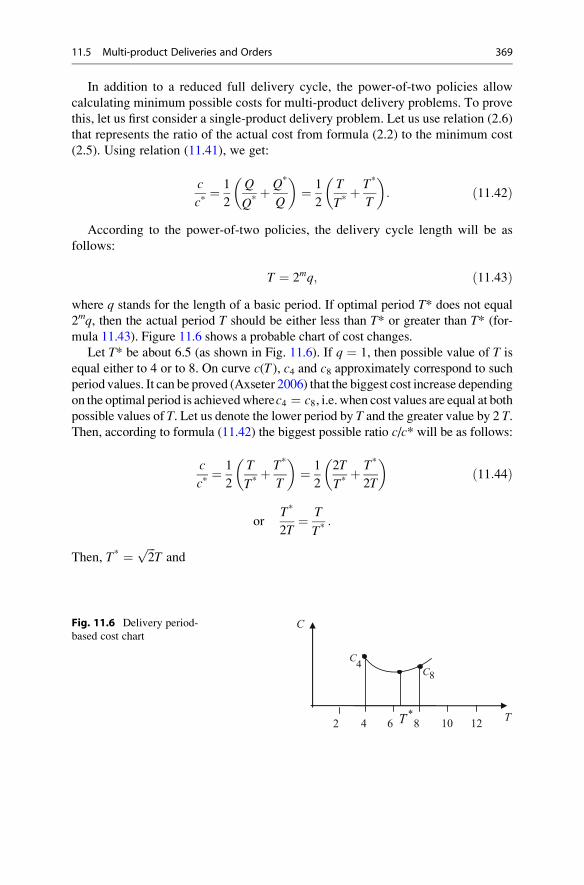
In addition to a reduced full delivery cycle, the power-of-two policies allow
calculating minimum possible costs for multi-product delivery problems. To prove
this, let us first consider a single-product delivery problem. Let us use relation (2.6)
that represents the ratio of the actual cost from formula (2.2) to the minimum cost
(2.5). Using relation (11.41), we get:
c
c*¼ 1
2
Q
Q*þ Q*
Q
� �¼ 1
2
T
T*þ T*
T
� �: ð11:42Þ
According to the power-of-two policies, the delivery cycle length will be as
follows:
T ¼ 2mq; ð11:43Þwhere q stands for the length of a basic period. If optimal period T* does not equal
2mq, then the actual period T should be either less than T* or greater than T* (for-
mula 11.43). Figure 11.6 shows a probable chart of cost changes.
Let T* be about 6.5 (as shown in Fig. 11.6). If q ¼ 1, then possible value of T is
equal either to 4 or to 8. On curve c(T), c4 and c8 approximately correspond to such
period values. It can be proved (Axseter 2006) that the biggest cost increase depending
on the optimal period is achievedwherec4 ¼ c8, i.e. when cost values are equal at bothpossible values of T. Let us denote the lower period by T and the greater value by 2 T.Then, according to formula (11.42) the biggest possible ratio c/c* will be as follows:
c
c*¼ 1
2
T
T*þ T*
T
� �¼ 1
2
2T
T*þ T*
2T
� �ð11:44Þ
orT*
2T¼ T
T*:
Then, T* ¼ ffiffiffi2
pT and
8C4
C
*T T
C
2 4 6 8 10 12
Fig. 11.6 Delivery period-
based cost chart
11.5 Multi-product Deliveries and Orders 369
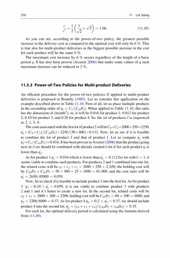
c
c*¼ 1
2
1ffiffiffi2
p þffiffiffi2
p� �¼ 1:06: ð11:45Þ
As you can see, according to the power-of-two policy, the greatest possible
increase in the delivery cost as compared to the optimal cost will only be 6 %. This
is true also for multi-product deliveries as the biggest possible increase in the cost
for each product will be the same 6 %.
The maximum cost increase by 6 % occurs regardless of the length of a basic
period q. It has also been proven (Axseter 2006) that under some values of q such
maximum increase can be reduced to 2 %.
11.5.3 Power-of-Two Policies for Multi-product Deliveries
An efficient procedure for the power-of-two policies if applied to multi-product
deliveries is proposed in Roundy (1985). Let us consider this application on the
example described above in Table 11.10. First of all, let us place multiple products
in the ascending order of ηi ¼ Ci= ChiDið Þ. When applied to Table 11.10, this ratio
has the dimension of (month2); so, it will be 0.016 for product 1; 0.012 for product
2; 0.10 for product 3, and 0.20 for product 4. So, the set of products J is sequencedas 2, 1, 3, 4.
The costs associatedwith the first lot of product 2will beC0þC2¼2000þ250¼2250;
η01¼ C0þC2ð Þ= Ch2D2ð Þ¼2250= 50�400ð Þ¼0:112. Now, let us see if it is feasible
to combine the lot of product 2 and that of product 1. Let us compare η01 with
η1¼C1= Ch1D1ð Þ¼0:016. It has been proven in Axseter (2006) that the product goingnext in J-set should be combined with already created k-lot if for such product ηi is
lower than η0k.
As for product 1 η1 ¼ 0:016 which is lower than η01 ¼ 0:112 for lot with k ¼ 1, it
seems viable to combine such products. For products 2 and 1 combined into one lot,
the related costs will be c0 þ c2 þ c1 ¼ 2000þ 250þ 2, 650, the holding cost will
be Ch2D2 þ Ch1D1 ¼ 50� 400þ 25� 1000 ¼ 45, 000, and the cost ratio will be
η01 ¼ 2650=45000 ¼ 0:059.Now, let us check if is feasible to include product 3 into the first lot. As for product
3 η3 ¼ 0:10 > η01 ¼ 0:059, it is not viable to combine product 3 with products
2 and 1 and it’s better to create a new lot. In the second lot, related costs will be
c0 þ c3 ¼ 2000þ 200 ¼ 2200, holding cost will beCh3D3 ¼ 60� 100 ¼ 6000, and
η03 ¼ 2200=6000 ¼ 0:37. As for product 4 η4 ¼ 0:2 < η
02 ¼ 0:37, we should include
product 4 into the second lot; η02 ¼ c0 þ c3 þ c4ð Þ= ch3D3 þ ch4D4ð Þ ¼ 0:35.
For each lot, the optimal delivery period is calculated using the formula derived
from (11.40).
370 11 Lot Sizing
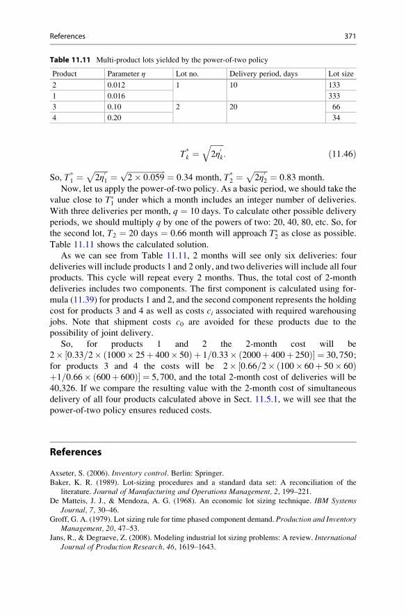
T*k ¼
ffiffiffiffiffiffiffi2η
0k
q: ð11:46Þ
So, T*1 ¼
ffiffiffiffiffiffiffi2η
01
p¼ ffiffiffiffiffiffiffiffiffiffiffiffiffiffiffiffiffiffiffiffi
2� 0:059p ¼ 0:34 month, T*
2 ¼ffiffiffiffiffiffiffi2η
02
p¼ 0:83 month.
Now, let us apply the power-of-two policy. As a basic period, we should take the
value close to T1 under which a month includes an integer number of deliveries.
With three deliveries per month, q ¼ 10 days. To calculate other possible delivery
periods, we should multiply q by one of the powers of two: 20, 40, 80, etc. So, for
the second lot, T2 ¼ 20 days ¼ 0.66 month will approach T2 as close as possible.Table 11.11 shows the calculated solution.
As we can see from Table 11.11, 2 months will see only six deliveries: four
deliveries will include products 1 and 2 only, and two deliveries will include all four
products. This cycle will repeat every 2 months. Thus, the total cost of 2-month
deliveries includes two components. The first component is calculated using for-
mula (11.39) for products 1 and 2, and the second component represents the holding
cost for products 3 and 4 as well as costs ci associated with required warehousing
jobs. Note that shipment costs c0 are avoided for these products due to the
possibility of joint delivery.
So, for products 1 and 2 the 2-month cost will be
2� 0:33=2� 1000� 25þ 400� 50ð Þ þ 1=0:33� 2000þ 400þ 250ð Þ½ � ¼ 30, 750;
for products 3 and 4 the costs will be 2� 0:66=2� 100� 60þ 50� 60ð Þ½þ1=0:66� 600þ 600ð Þ� ¼ 5, 700, and the total 2-month cost of deliveries will be
40,326. If we compare the resulting value with the 2-month cost of simultaneous
delivery of all four products calculated above in Sect. 11.5.1, we will see that the
power-of-two policy ensures reduced costs.
References
Axseter, S. (2006). Inventory control. Berlin: Springer.Baker, K. R. (1989). Lot-sizing procedures and a standard data set: A reconciliation of the
literature. Journal of Manufacturing and Operations Management, 2, 199–221.De Matteis, J. J., & Mendoza, A. G. (1968). An economic lot sizing technique. IBM Systems
Journal, 7, 30–46.Groff, G. A. (1979). Lot sizing rule for time phased component demand. Production and Inventory
Management, 20, 47–53.Jans, R., & Degraeve, Z. (2008). Modeling industrial lot sizing problems: A review. International
Journal of Production Research, 46, 1619–1643.
Table 11.11 Multi-product lots yielded by the power-of-two policy
Product Parameter η Lot no. Delivery period, days Lot size
2 0.012 1 10 133
1 0.016 333
3 0.10 2 20 66
4 0.20 34
References 371
Lukinsky, V. S. (2007). Logistic models and methods. Saint Petersburg: Piter (in Russian).
Mauergauz, Y. E. (2007). Automated dynamic planning in machinery industry. Moscow:
Economika (in Russian).
Nydick, R. L., & Weiss, H. J. (1989). An evaluation of variable demand lot sizing techniques.
Production and Inventory Management, 30, 41–44.Roundy, R. (1985). 98%-Effective integer-ratio lot-sizing for one-warehouse multi-retailer
systems. Management Science, 31, 1416–1430.Ryzhikov, Y. I. (2001). Queuing theory and inventory management. St. Petersburg: Piter
(in Russian).
Sachko, N. S. (2008). Management and control in machinery industry. Minsk: Novoye Znanie
(in Russian).
Silver, E. A., & Meal, H. C. (1973). A heuristic for selecting lot size requirements for the case of a
deterministic time-varying demand rate and discrete opportunities for replenishment. Produc-tion and Inventory Management, 14, 64–74.
Sterligova, A. N. (2006). Inventory management in supply chains. Moscow: Infra-M (in Russian).
Tanaev, V. S., Kovalev, M. Y., & Shafransky, Y. M. (1998). Scheduling theory. GroupTechnologies. Institute of Engineering Cybernetics, National Academy of Science, Minsk,
Belarus (in Russian).
Wagner, H. M., & Whitin, T. M. (1958). Dynamic version of the economic lot size model.
Management Science, 5, 89–96.
372 11 Lot Sizing
Production Planning 12
12.1 Master Production Planning
The objective of the master planning, as is well known, is transformation of existing
demand forecasts and orders of an enterprise into a specific plan of action for certain
near period. The master plan may be drawn up directly according to the forecasts
and orders, and can be elaborated based on the existing sales and operations plan,
and the latter is preferred. The master plan unlike the sales and operations plan is
much more detailed, i.e. aggregation of individual products here is the exception
rather than the rule.
The master plan is a set of planning items that should be produced within several
planning periods from the beginning of this plan to the planning horizon. A planning
period is as a rule 1 month and with large-scale production—1 week. The horizon of
the master planning can be set within 3�12 planning periods depending on what theproduct’s position in themarket is (Sect. 1.6.1). If themarket is stable, meaning there
is a balance of supply and demand (Fig. 10.1), then it is reasonable to carry out
planning with the greatest horizon, and in all other cases, the horizon should be less.
With various types of production, planning stages, and methods of analysis of
elaborated plans, it is convenient to use various planning items. The use of computers
allows parallel planning simultaneously on several planning items. In this approach,
duringmodelling of the production process the user is able to transfer from analysis of
major planning items to a more detailed analysis of their constituents and make a
well-reasoned decision.
The planning items used in the planning system can be presented as a hierarchi-
cal tree, on the lower level of which apparently there is a technological operation. It
is much more difficult to set a rational planning item of the highest level.
In the make-to-stock production, this kind of item is usually represented by a
particular type of finished products. With make-to-order strategy, it seems quite
natural to use external orders as planning items. Using an external order as a
planning item is convenient in terms of production and financial accounting, but
# Springer International Publishing Switzerland 2016
Y. Mauergauz, Advanced Planning and Scheduling in Manufacturing and SupplyChains, DOI 10.1007/978-3-319-27523-9_12
373
has a very significant drawback—job-order production leads to small lot sizes and
significant increase in cost.
12.1.1 Master Planning as Product Tables
This way of presenting the master plan is mainly used when the demand can be
forecasted well for the product and it enables “make-to-stock” strategy (Vollmann
et al. 2005). For each such product a table is drawn up that shows the demand
forecast, output plan, and current stock level for each planning period within the
horizon.
Such a table for the simplest case has the form shown in (Table 12.1). The volume
of the product, its receipt at the storage, and issue from the storage are calculated at
the end of a period. Table 12.1 shows the case of the standing production of the
product and the forecast having a peak demand in the area of the fourth and fifth
weeks. The presented production plan tracks the probable peak demand in advance
and then the output is reduced in order to restore the initial stock level. This variant is
typical for the production with a short production cycle, operating in a stable market
subject to seasonal fluctuations.
A more complex version is shown in Table 12.2. Here the demand forecast tends
to grow. The product is manufactured in batches of fixed size (Sect. 8.2.1) and the
production cycle is 2 weeks. As a result, the stock varies considerably and may even
lead to the unsatisfied demand.
When using the model with fixed supply period (Sect. 8.2.2) and duration of the
production cycle of 3 weeks the product planning takes the form presented in
Table 12.3. The down trend of the demand leads to a reduced lot size in this model.
In developing the master plan the division workload should be checked more in
detail than in preparation of the sales and operations plan (Sect. 10.1.2). In the
literature, for this purpose it is recommended to use the so-called resource profile
method described in Fogarty et al. (1993). This method is quite acceptable; how-
ever, to use it, it is necessary to have data on the division workload for each time
period until the completion of the batch.
More often, we know the capacity of each division or work center with high
workload for each planned product, as well as operation lead in this division and
their duration (Table 12.4). In Table 12.4 it is assumed that products B2 and B3 are
processed in division A2 right after processing in division A1.
The capacity of a division is understood here as the amount of the product
processed or manufactured per day when other products are not produced at this
time. A rough estimate of the capacity on the product can be obtained by simply
dividing the daily time fund of the production divisions by processing time of the
unit of the product measure in this division.
If several products are produced during the same period, the production of each
of them uses a relevant share of the total division’s capacity. For example, with
the planned output of product B1 for week 1 amounting to 1000 UM (Table 12.1)
and the length of the working week equal to 5 working days, the consumed part of
374 12 Production Planning
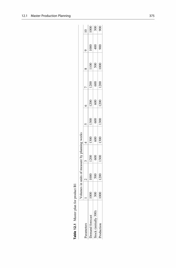
Table
12.1
Masterplanforproduct
B1
Param
eters
Volumes
inunitsofmeasure
byplanningweeks
12
34
56
78
910
Dem
andforecast
1000
1000
1200
1300
1300
1200
1200
1100
1000
1000
Stock
(initially300)
300
500
600
600
600
600
600
500
400
300
Production
1000
1200
1300
1300
1300
1200
1200
1000
900
900
12.1 Master Production Planning 375
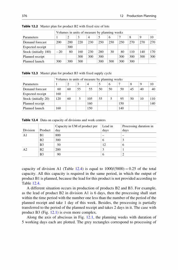
capacity of division A1 (Table 12.4) is equal to 1000/(5800)¼ 0.25 of the total
capacity. All this capacity is required in the same period, in which the output of
product B1 is planned, because the lead for this product is not provided according to
Table 12.4.
A different situation occurs in production of products B2 and B3. For example,
as the lead of product B2 in division A1 is 6 days, then the processing shall start
within the time period with the number one less than the number of the period of the
planned receipt and take 1 day of this week. Besides, the processing is partially
transferred to the period of the planned receipt and takes 2 days in it. The case with
product B3 (Fig. 12.1) is even more complex.
Along the axis of abscissas in Fig. 12.1, the planning weeks with duration of
5 working days each are plotted. The grey rectangles correspond to processing of
Table 12.2 Master plan for product B2 with fixed size of lots
Parameters
Volumes in units of measure by planning weeks
1 2 3 4 5 6 7 8 9 10
Demand forecast 200 200 220 230 250 250 250 270 270 270
Expected receipt 300
Stock (initially 180) �20 80 160 230 280 30 80 110 140 170
Planned receipt 300 300 300 300 300 300 300
Planned launch 300 300 300 300 300 300 300
Table 12.3 Master plan for product B3 with fixed supply cycle
Parameters
Volumes in units of measure by planning weeks
1 2 3 4 5 6 7 8 9 10
Demand forecast 60 60 55 55 50 50 50 45 40 40
Expected receipt 160
Stock (initially 20) 120 60 5 105 55 5 95 50 10 110
Planned receipt 160 150 140
Planned launch 160 150 140
Table 12.4 Data on capacity of divisions and work centers
Division Product
Capacity in UM of product per
day
Lead in
days
Processing duration in
days
A1 B1 800 – –
B2 300 6 3
B3 50 12 6
A2 B2 200 3 1
B3 90 6 2
376 12 Production Planning
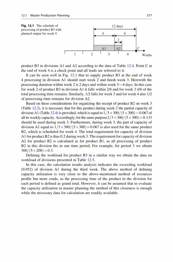
product B3 in divisions A1 and A2 according to the data of Table 12.4. Point C at
the end of week 4 is a check point and all leads are referred to it.
It can be seen well in Fig. 12.1 that to supply product B3 at the end of week
4 processing in division A1 should start week 2 and finish week 3. Herewith the
processing duration within week 2 is 2 days and within week 3—4 days. In this case
for week 2 of product B3 in division A1 it falls within 2/6 and for week 3 4/6 of the
total processing time remains. Similarly, 1/2 falls for week 3 and for week 4 also 1/2
of processing time remains for division A2.
Based on these considerations for organizing the receipt of product B2 on week 3
(Table 12.2), it is necessary that for this product during week 2 the partial capacity of
division A1 (Table 12.4) is provided, which is equal to 1=3�300= 5�300ð Þ¼0:067 ofall itsweekly capacity.Accordingly, for the same purpose2=3�300= 5�300ð Þ¼0:133should be used during week 3. Furthermore, during week 3, the part of capacity of
division A1 equal to 1=3�300= 5�300ð Þ¼0:067 is also used for the same product
B2, which is scheduled for week 4. The total requirement for capacity of division
A1 for product B2 is thus 0.2 duringweek 3. The requirement for capacity of division
A2 for product B2 is calculated as for product B1, as all processing of product
B2 in this division fits in one time period. For example, for period 3 we obtain
300= 5�200ð Þ¼0:3.Defining the workload for product B3 in a similar way we obtain the data on
workload of divisions presented in Table 12.5.
In this case, the calculation results analysis indicates the exceeding workload
(0.952) of division A1 during the third week. The above method of defining
capacity utilization is very close to the above-mentioned method of resources
profile but more crude, as the processing time of the product in the division for
each period is defined as grand total. However, it can be assumed that to evaluate
the capacity utilization in master planning the method of this closeness is enough
while the necessary data for calculation are readily available.
С
2
66
Weeks21 3 4
A1 A2
12 daysFig. 12.1 The schedule of
processing of product B3 with
planned output for week 4
12.1 Master Production Planning 377
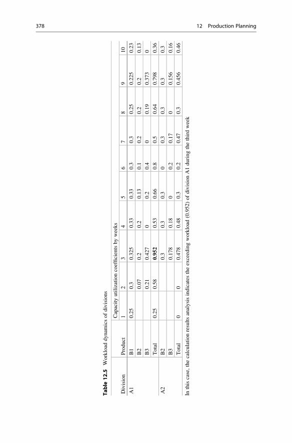
Table
12.5
Workload
dynam
icsofdivisions
Division
Product
Capacityutilizationcoefficientsbyweeks
12
34
56
78
910
A1
B1
0.25
0.3
0.325
0.33
0.33
0.3
0.3
0.25
0.225
0.23
B2
0.07
0.2
0.2
0.13
0.1
0.2
0.2
0.2
0.13
B3
0.21
0.427
00.2
0.4
00.19
0.373
0
Total
0.25
0.58
0.95
20.53
0.66
0.8
0.5
0.64
0.798
0.36
A2
B2
0.3
0.3
0.3
00.3
0.3
0.3
0.3
B3
0.178
0.18
00.2
0.17
00.156
0.16
Total
00
0.478
0.48
0.3
0.2
0.47
0.3
0.456
0.46
Inthiscase,thecalculationresultsanalysisindicates
theexceedingworkload
(0.952)ofdivisionA1duringthethirdweek
378 12 Production Planning

12.1.2 Group Master Planning
When operating in the volatilemarket both the demand forecast and its actual error are
subject to great fluctuations. In these cases, of course, every company strives to make-
to-order operation. However, with sufficiently long production cycle the operation
strategy only under orders increases the waiting period of the order, which reduces the
competitiveness of the enterprise.
Therefore, in some cases it is advisable to produce some portion of all products
using make-to-order strategy and some portion using make-to-stock or assembly-
to-order strategy (Sect. 1.3.2). Anyway, it makes sense to assume that the entire
production output is made by orders, but the part of this output is fulfilled as the
internal order of the enterprise. Herewith the planning is virtually always performed
for a certain jointly processed group of external and internal orders, and in the
particular case such a group may consist of only one order.
In many information systems the group of orders intended for joint processing is
considered to be a planning item (PI) and called a production order. However, this
term is quite overloaded and mostly belongs to the financial and economic activity.
For this reason, (Mauergauz 2007) it is suggested to use also term “planning group”
for such a group of orders.
Wewill understand a planning group as a set of some finished products and spareparts launched into production simultaneously. It is reasonable to include products
of different types with a close design-engineering composition as well as spare parts
similar to some components of these products into this set.
The number of products and parts of each type in the planning group should be
established based on rational stock quantity at all times during production of the
planning group. The production and marketing time of the planning group and,
accordingly, the size of the planning group are determined by the planning horizon
of the manufactured products. The output of products belonging to one planning
group can be performed gradually within several planning periods. One planning
group can provide fulfilment of a number of orders or their separate stages.
Using a planning group as a basic PI allows setting quite large sizes of produc-
tion lots since each lot of parts, assemblies, components, and finished products is
produced not for one order and not even for one planning period but to provide for
the established planning group.
The planning group differentiates release lots and output lots of products and
their components. On the ground of the planning group definition, there is only one
release lot of products of each type, which together form a launch group.
At the same time, there may be several output lots of the same type of products.
The completion time of output lots may relate to different time periods, and the
output lot sizes are set either by the available capacity of the assembly production or
by the expected requirement for products for sales. Each output lot of products in
the planning group is a planning item in the hierarchy below the planning group and
type of product. Set of output lots of products of the same type within the planning
group is a line of these products.
12.1 Master Production Planning 379
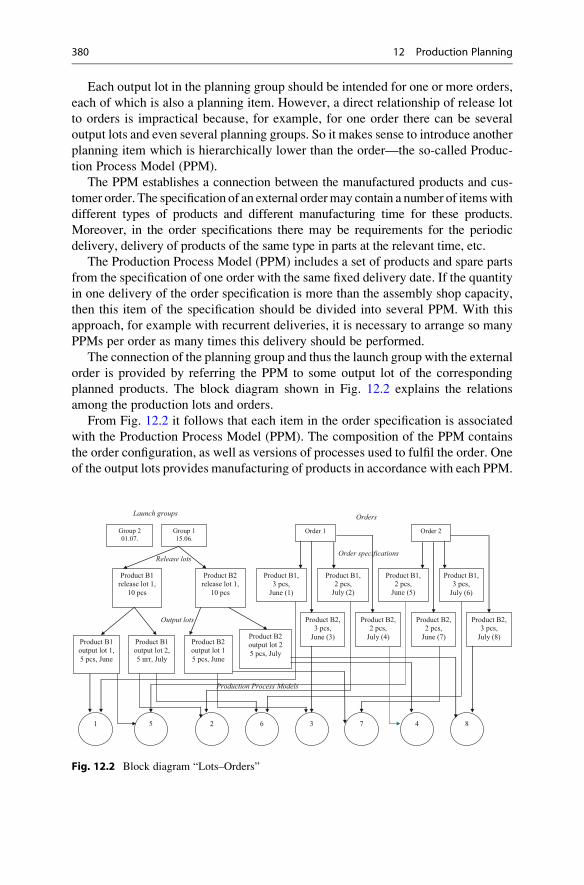
Each output lot in the planning group should be intended for one or more orders,
each of which is also a planning item. However, a direct relationship of release lot
to orders is impractical because, for example, for one order there can be several
output lots and even several planning groups. So it makes sense to introduce another
planning item which is hierarchically lower than the order—the so-called Produc-
tion Process Model (PPM).
The PPM establishes a connection between the manufactured products and cus-
tomer order. The specification of an external ordermay contain a number of itemswith
different types of products and different manufacturing time for these products.
Moreover, in the order specifications there may be requirements for the periodic
delivery, delivery of products of the same type in parts at the relevant time, etc.
The Production Process Model (PPM) includes a set of products and spare parts
from the specification of one order with the same fixed delivery date. If the quantity
in one delivery of the order specification is more than the assembly shop capacity,
then this item of the specification should be divided into several PPM. With this
approach, for example with recurrent deliveries, it is necessary to arrange so many
PPMs per order as many times this delivery should be performed.
The connection of the planning group and thus the launch group with the external
order is provided by referring the PPM to some output lot of the corresponding
planned products. The block diagram shown in Fig. 12.2 explains the relations
among the production lots and orders.
From Fig. 12.2 it follows that each item in the order specification is associated
with the Production Process Model (PPM). The composition of the PPM contains
the order configuration, as well as versions of processes used to fulfil the order. One
of the output lots provides manufacturing of products in accordance with each PPM.
Group 201.07.
Launch groups
Group 115.06.
Product B1release lot 1,
10 pcs
Product B2release lot 1,
10 pcs
Release lots
Product B1output lot 1,
5 pcs, June
Output lots
Product B1output lot 2,
5 шт, July
Product B2output lot 1
5 pcs, June
Product B2output lot 2
5 pcs, July
Order 1
Orders
Order 2
Order specifications
Product B1, 3 pcs,
June (1)
Product B1, 2 pcs,
July (2)
Product B2, 2 pcs,
July (4)
Product B1, 2 pcs,
June (5)
Product B1, 3 pcs,
July (6)
Product B2,2 pcs,
June (7)
Product B2, 3 pcs,
June (3)
Product B2, 3 pcs,
July (8)
Production Process Models
1 5 2 6 3 7 4 8
Fig. 12.2 Block diagram “Lots–Orders”
380 12 Production Planning
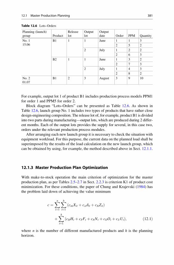
For example, output lot 1 of product B1 includes production process models PPM1
for order 1 and PPM5 for order 2.
Block diagram “Lots–Orders” can be presented as Table 12.6. As shown in
Table 12.6, launch group No. 1 includes two types of products that have rather close
design-engineering composition. The release lot of, for example, product B1 is divided
into two parts during manufacturing—output lots, which are produced during 2 differ-
ent months. Each of the output lots provides the supply for several, in this case two,
orders under the relevant production process modules.
After arranging each new launch group it is necessary to check the situation with
equipment workload. For this purpose, the current data on the planned load shall be
superimposed by the results of the load calculation on the new launch group, which
can be obtained by using, for example, the method described above in Sect. 12.1.1.
12.1.3 Master Production Plan Optimization
With make-to-stock operation the main criterion of optimization for the master
production plan, as per Tables 2.5–2.7 in Sect. 2.2.3 is criterion K1 of product cost
minimization. For these conditions, the paper of Chung and Krajevski (1984) has
the problem laid down of achieving the value minimum
c ¼Xni¼1
Xht¼1
cmiXit þ coiδit þ chiZitð Þ
þXht¼1
cHHt þ cFFt þ cNNt þ cOOt þ cUUtð Þ; ð12:1Þ
where n is the number of different manufactured products and h is the planning
horizon.
Table 12.6 Lots–Orders
Planning (launch)
group Product
Release
lot
Output
lot
Output
date Order PPM Quantity
No. 1
15.06
B1 1 1 June 1 1 3
2 5 2
2 July 1 2 2
2 6 3
B2 1 1 June 1 3 2
2 7 3
2 July 1 4 3
2 8 2
No. 2
01.07
B1 2 3 August 3 9 10
12.1 Master Production Planning 381
The costs in Eq. (12.1): cmi—the production cost of the unit of measure of the
i-th product; coi—the cost of regular setup of production to start operation in the
period; chi—the storage cost of the unit of measure during one period; cH—the cost
of hiring per person; cF—the cost of firing per person; cX—the cost of materials per
product unit; cN—period average salary of one employee in normal; conditions;
cO—the cost of overtime hour; cZ—the cost of storage per product unit; cU—the cost
of production downtime per hour.
For each i-th product in Eq. (12.1), the following is included: Xit—the quantity of
product manufactured within period t in hours; δit—binary variable defining the fact
of setup in period t; Zit—the quantity of product in stock by the end of period t. InEq. (12.1) it is also specified: Ht—the number of newly hired employees; Ft—the
number of fired employees; Nt—the current number of employees; Ot—number of
overtime hours; Ut—number of downtime hours.
The first constraint is the constraint in stocks which is the set of equations
Zit ¼ Zi, t�1 þ Xit � Dit with 1 � i � n, 1 � t � h: ð12:2ÞThe personnel balance is
Nt ¼ Nt�1 þ Ht � Ft forall 1 � t � h: ð12:3ÞThe working time balance is
GNt þ Ot �Xni¼1
Xit �Xni¼1
Siδit � 0 forall 1 � t � h; ð12:4Þ
where G is the time fund in hours of one employee within the period with regular
payment;
Si the duration of setup for the i-th product.
The constraint for the overtime
Ot � BNt forall 1 � t � h; ð12:5Þwhere B is the allowable overtime hours for one employee within the period.
The constraint on the quantity of product has the form of inequation system
Xit � M � δit with 1 � i � n, 1 � t � h; ð12:6Þwhere “big” number M is defined from expression (11.8).
Variables of setup
δit ¼ 1 with Xit > 0 and δit ¼ 0 and Xit ¼ 0: ð12:7ÞRequirement for the safety stock Zci at the end of each period
382 12 Production Planning
Zit � Zci with 1 � i � n, 1 � t � h : ð12:8ÞThe variables in expression (12.1)–(12.8) are the output of product Xit, the fact of
setup for product δit, the number of fired employeesFt, the number of hired employees
Ht, and the number of overtime hours Ot.
The problem stated in the form of objective function (Eq. 12.1) and constraints
(Eqs. 12.2 and 12.3) is actually a combination of the problem set for one aggregate
group in Sect. 10.2.1 and the problem of the lot sizes with capacity constraints and
large planning interval described in Sect. 11.1.3.
The solution of the problems of this type, as was shown above, is possible by MS
Excel techniques, but at that, the number of variables becomes considerable. For
example, in the book of Shapiro (2001), the problems with the 13-week (3-month)
planning for 500 different products are discussed. A problem of this size requires 6500
binary variables 0–1, wherein the amount of the remaining problem’s constraints
reaches 20,000. Since the direct solution in such cases is difficult to obtain, Shapiro
(2001) proposes to use the method of the so-called decomposition in which several
possible plans are considered successively and the best of them is selected.
As such possible plans, usually the plans optimizing the initial problem in a small
interval of time (for example, 1 week) are accepted. With the set of plans available
for several periods ahead, we can agree them consistently and thus obtain a unified
plan for the period up to the planning horizon.
With make-to-order operation, the quality criteria of the master plan, as shown in
Tables 2.5–2.7, change. In this case, besides the product costs, it is necessary to
consider the timing of order fulfilment as well and so the optimization problem
becomes multi-objective and cannot be solved by linear programming techniques.
The use of group scheduling allows calculating (Mauergauz 2007) the values of the
quality criteria such as the full output, profit, necessary working capital, capacity
utilization, penalties for non-fulfilment of contracts, duration of the contracts
performance, etc., for each elaborated plan option. Using the utility functions of
each criterion (Sect. 1.7.2) we can define the integral characteristic of each option
and choose the best.
12.2 Material Requirement Planning
To produce complex products consisting of several or many components, the produc-
tion planning of the latter is carried out in accordance with the developedmaster plan.
These components are objects of dependent demand, i.e. their bill ofmaterials (BOM)
can be directly calculated in terms of the master plan. The manufacturing resource
planning (MRP2) is an essential element of modern production management, and its
core is a set of planning tables of each component similar to Table 12.2 or 12.3 for the
master plan (Sect. 12.1.1). Table 2.12 refers to the so-called order policy with a fixed
size of an order, and Table 12.3 refers to the order policy with a fixed cycle.
12.2 Material Requirement Planning 383
The most difficult issue of material requirement planning is the definition of
rational production lot sizes. First of all, the components lots should be sufficient to
assemble the planned lots of finished products, i.e. the minimum lot size of com-
ponents is determined by one lot of finished products. This option is applied with
lot-for-lot order policy. However, since with such a relevance the lots of com-
ponents often get small and thus expensive, the components lot sizes are necessary
to be increased.
The second issue is to determine the duration of lot production. While develop-
ing the master plan (Table 12.3), the dependence of the lot lead time on its size, in
some range, is often overlooked, because the duration of the production cycle of the
finished product is taken with a large margin against the duration of the process
cycle. However, in manufacturing of components it is no longer possible to neglect
this dependence.
Generally speaking, the lot size of components should meet the demand for a
certain number of time periods, but as the lead time depends on the size of the lot,
the moment of the lot receipt becomes variable. The result is that it is not always
clear whether the lot can meet the demand for the selected number of time periods,
i.e. when using Table 12.3 we face a vicious circle.
It is possible to eliminate this disadvantage of planning in MRP2, if we use the
“planning group” policy of orders. By definition of the planning group in Sect. 12.1.2,
each planning group corresponds to one launch group of finished products and spare
parts of multiple types. Table 12.6 “Lots–Orders” is a sequence of planning (launch)
groups providing fulfilment of external and internal orders. The “planning group”
policy of orders as applied to Table 12.6 is a generalization of “lot-to-lot” policy, in
which the lot of finished product is a planning group. At the same time, the com-
ponents release lots corresponding exactly to the launch group and the components
output lots must ensure the output lots of the planning group.
12.2.1 Production Lot Duration
The total production time of the i-th product lot (production cycle Fi) is determined
by the time of its processing and transfer time between divisions and between
operations within the divisions. Furthermore, it is sometimes necessary to provide
time for the natural maturing (ageing, drying, etc.). The lot processing time (planned
job) is equal to
p ¼ sþ Qτ; ð12:9Þwhere s is the total setup time for the operations, Q—lot size, and τ—full run time
of processing. Duration of processing may differ from value determined by formula
(12.9) in the cases of the so-called parallel processing, in which one or more
operations of a lot is handled simultaneously on several machines.
In general, with sequential flow of the processed product the production time of a
lot with n operations
384 12 Production Planning
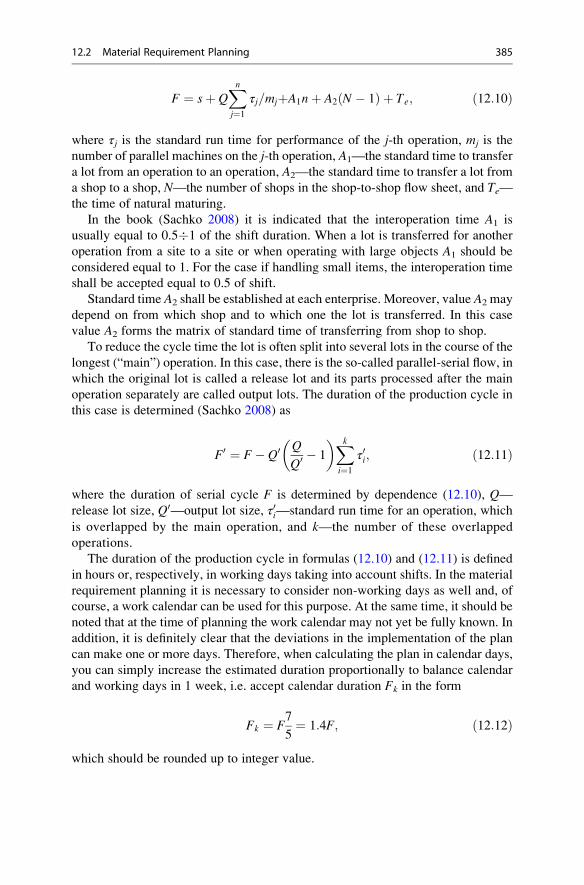
F ¼ sþ QXnj¼1
τj=mjþA1nþ A2 N � 1ð Þ þ Te; ð12:10Þ
where τj is the standard run time for performance of the j-th operation, mj is the
number of parallel machines on the j-th operation, A1—the standard time to transfer
a lot from an operation to an operation, A2—the standard time to transfer a lot from
a shop to a shop, N—the number of shops in the shop-to-shop flow sheet, and Te—the time of natural maturing.
In the book (Sachko 2008) it is indicated that the interoperation time A1 is
usually equal to 0.5�1 of the shift duration. When a lot is transferred for another
operation from a site to a site or when operating with large objects A1 should be
considered equal to 1. For the case if handling small items, the interoperation time
shall be accepted equal to 0.5 of shift.
Standard time A2 shall be established at each enterprise. Moreover, value A2 may
depend on from which shop and to which one the lot is transferred. In this case
value A2 forms the matrix of standard time of transferring from shop to shop.
To reduce the cycle time the lot is often split into several lots in the course of the
longest (“main”) operation. In this case, there is the so-called parallel-serial flow, in
which the original lot is called a release lot and its parts processed after the main
operation separately are called output lots. The duration of the production cycle in
this case is determined (Sachko 2008) as
F0 ¼ F� Q0 Q
Q0 � 1
� �Xki¼1
τ0i; ð12:11Þ
where the duration of serial cycle F is determined by dependence (12.10), Q—release lot size, Q0—output lot size, τ0i—standard run time for an operation, which
is overlapped by the main operation, and k—the number of these overlapped
operations.
The duration of the production cycle in formulas (12.10) and (12.11) is defined
in hours or, respectively, in working days taking into account shifts. In the material
requirement planning it is necessary to consider non-working days as well and, of
course, a work calendar can be used for this purpose. At the same time, it should be
noted that at the time of planning the work calendar may not yet be fully known. In
addition, it is definitely clear that the deviations in the implementation of the plan
can make one or more days. Therefore, when calculating the plan in calendar days,
you can simply increase the estimated duration proportionally to balance calendar
and working days in 1 week, i.e. accept calendar duration Fk in the form
Fk ¼ F7
5¼ 1:4F; ð12:12Þ
which should be rounded up to integer value.
12.2 Material Requirement Planning 385
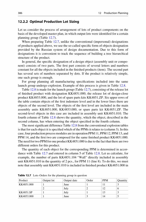
12.2.2 Optimal Production Lot Sizing
Let us consider the process of arrangement of lots of product components on the
basis of the developed master plan, in which output lots were identified for a certain
planning group (Table 12.7).
When preparing Table 12.7, unlike the conventional (impersonal) designations
of products applied above, we use the so-called specific form of objects designation
provided by the Russian system of design documentation. Due to this form of
designations it is convenient to track the sequence of building a tree hierarchical
structure of the product.
In general, the specific designation of a design object (assembly unit or compo-
nent) consists of two parts. The first part consists of several letters and numbers
constant for all the objects included in the finished products (item). The second part
has several sets of numbers separated by dots. If the product is relatively simple,
one such group is enough.
For group planning all manufacturing specifications included into the same
launch group undergo explosion. Example of this process is given in Table 12.8.
Table 12.8 is made for the launch group (Table 12.7), consisting of the release lot
of finished product with designation KK4851.000, the release lot of design-close
product KK4853.000, and the lot of spare parts kits KK4851.ZP. Six upper rows of
the table contain objects of the first indenture level and in the lower lines there are
objects of the second level. The objects of the first level are included in the main
assembly units KK4851.000, KK4853.000, or spare parts kit KK4851.ZP. The
second-level objects in this case are included in assembly unit KK4851.010. The
fourth column of Table 12.8 shows the quantity, which the object, described in the
second column, has when entering the object specified in the fourth column.
The most significant difference Table 12.8 from the conventional explosion tables
is that for each object it is specified which of the PPMs it relates to (column 3). In this
case, four production processmodules are in operation PPM11, PPM12, PPM13, and
PPM 14, and the first two are composed for the same finished product KK4851.000.
The need for twoPPM for one productKK4851.000 is due to the fact that there are two
different orders for this product.
The quantity of each object for the corresponding PPM is determined in accor-
dance with Table 12.7 and entered in column 5 of Table 12.8. Let us calculate, for
example, the number of parts KK4851.104 “Wall” directly included in assembly
unit KK4851.010 in the quantity of 2 pcs., for PPM 11 (line 8). To do this, we must
note that assembly unit KK4851.010 is included in finished product KK4851.000 in
Table 12.7 Lots–Orders for the planning group in question
Product Output lot Output date Order PPM Quantity
KK4851.000 1 June 1 11 3
2 July 2 12 6
KK4851.SP 1 July 1 13 3
KK4853.000 1 June 3 14 5
386 12 Production Planning
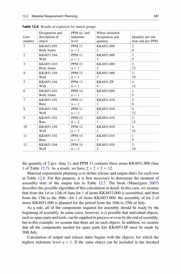
the quantity of 2 pcs. (line 1), and PPM 11 contains three items KK4851.000 (line
1 of Table 12.7). As a result, we have 2� 2� 3 ¼ 12.
Material requirement planning is to define release and output dates for each row
in Table 12.8. For this purpose, it is first necessary to determine the moment of
assembly start of the output lots in Table 12.7. The book (Mauergauz 2007)
describes the possible algorithm of this calculation in detail. In this case, we assume
that from the 1st to 12th of June lot 1 of items KK4853.000 is assembled, and then
from the 13th to the 30th—lot 1 of items KK4853.000; the assembly of lot 2 of
items KK4851.000 is planned for the period from the 10th to 25th of July.
As a rule, all of the components required for assembly should be ready by the
beginning of assembly. In some cases, however, it is possible that individual objects,
such as spare parts and tools, can be supplied in process or even by the end of assembly,
but in this example, we assume that there are no such objects. In addition, we assume
that all the components needed for spare parts kits KK4853.SP must be made by
30th July.
Calculation of output and release dates begins with the objects, for which the
highest indenture level u ¼ 1. If the same object can be included in the finished
Table 12.8 Results of explosion for launch groups
Line
number
Designation and
description of
object
PPM no. and
indenture
level
Where included:
designation and
quantity
Quantity per one
item and per PPM
1 KK4851.010
Body frame
PPM 11
u ¼ 1
KK4851.000
2
2
6
2 KK4851.104
Wall
PPM 11
u ¼ 1
KK4851.000
3
3
9
3 KK4851.010
Body frame
PPM 12
u ¼ 1
KK4851.000
2
2
12
4 KK4851.104
Wall
PPM 12
u ¼ 1
KK4851.000
3
3
18
5 KK4851.104
Wall
PPM 13
u ¼ 1
KK4851.ZP
4
4
12
6 KK4851.010
Body frame
PPM 14
u ¼ 1
KK4853.000
1
1
5
7 KK4851.102
Base
PPM 11
u ¼ 2
KK4851.010
1
2
6
8 KK4851.104
Wall
PPM 11
u ¼ 2
KK4851.010
2
4
12
9 KK4851.102
Base
PPM 12
u ¼ 2
KK4851.010
1
2
12
10 KK4851.104
Wall
PPM 12
u ¼ 2
KK4851.010
2
4
24
11 KK4851.102
Base
PPM 14
u ¼ 2
KK4851.010
1
1
5
12 KK4851.104
Wall
PPM 14
u ¼ 2
KK4851.010
2
2
10
12.2 Material Requirement Planning 387
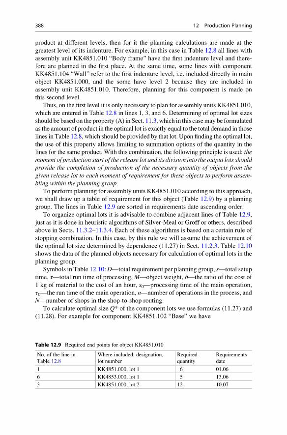
product at different levels, then for it the planning calculations are made at the
greatest level of its indenture. For example, in this case in Table 12.8 all lines with
assembly unit KK4851.010 “Body frame” have the first indenture level and there-
fore are planned in the first place. At the same time, some lines with component
KK4851.104 “Wall” refer to the first indenture level, i.e. included directly in main
object KK4851.000, and the some have level 2 because they are included in
assembly unit KK4851.010. Therefore, planning for this component is made on
this second level.
Thus, on the first level it is only necessary to plan for assembly units KK4851.010,
which are entered in Table 12.8 in lines 1, 3, and 6. Determining of optimal lot sizes
should be based on the property (A) in Sect. 11.3, which in this casemay be formulated
as the amount of product in the optimal lot is exactly equal to the total demand in those
lines in Table 12.8, which should be provided by that lot. Upon finding the optimal lot,
the use of this property allows limiting to summation options of the quantity in the
lines for the same product. With this combination, the following principle is used: themoment of production start of the release lot and its division into the output lots shouldprovide the completion of production of the necessary quantity of objects from thegiven release lot to each moment of requirement for these objects to perform assem-bling within the planning group.
To perform planning for assembly units KK4851.010 according to this approach,
we shall draw up a table of requirement for this object (Table 12.9) by a planning
group. The lines in Table 12.9 are sorted in requirements date ascending order.
To organize optimal lots it is advisable to combine adjacent lines of Table 12.9,
just as it is done in heuristic algorithms of Silver-Meal or Groff or others, described
above in Sects. 11.3.2–11.3.4. Each of these algorithms is based on a certain rule of
stopping combination. In this case, by this rule we will assume the achievement of
the optimal lot size determined by dependence (11.27) in Sect. 11.2.3. Table 12.10
shows the data of the planned objects necessary for calculation of optimal lots in the
planning group.
Symbols in Table 12.10:D—total requirement per planning group, s—total setup
time, τ—total run time of processing,M—object weight, b—the ratio of the cost of
1 kg of material to the cost of an hour, s0—processing time of the main operation,
τ0—the run time of the main operation, n—number of operations in the process, and
N—number of shops in the shop-to-shop routing.
To calculate optimal size Q* of the component lots we use formulas (11.27) and
(11.28). For example for component KK4851.102 “Base” we have
Table 12.9 Required end points for object KK4851.010
No. of the line in
Table 12.8
Where included: designation,
lot number
Required
quantity
Requirements
date
1 KK4851.000, lot 1 6 01.06
6 KK4853.000, lot 1 5 13.06
3 KK4851.000, lot 2 12 10.07
388 12 Production Planning
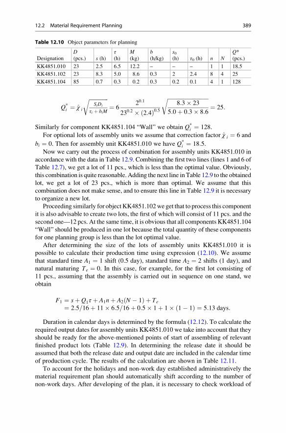
Q*i ¼ χ i
ffiffiffiffiffiffiffiffiffiffiffiffiffiffiSiDi
τi þ biM
r¼ 6
20:1
230:2 � 2:4ð Þ0:5ffiffiffiffiffiffiffiffiffiffiffiffiffiffiffiffiffiffiffiffiffiffiffiffiffiffiffiffiffiffi
8:3� 23
5:0þ 0:3� 8:6
r¼ 25:
Similarly for component KK4851.104 “Wall” we obtain Q*i ¼ 128.
For optional lots of assembly units we assume that correction factor χ i ¼ 6 and
bi ¼ 0. Then for assembly unit KK4851.010 we have Q*i ¼ 18:5.
Now we carry out the process of combination for assembly units KK4851.010 in
accordance with the data in Table 12.9. Combining the first two lines (lines 1 and 6 of
Table 12.7), we get a lot of 11 pcs., which is less than the optimal value. Obviously,
this combination is quite reasonable. Adding the next line in Table 12.9 to the obtained
lot, we get a lot of 23 pcs., which is more than optimal. We assume that this
combination does not make sense, and to ensure this line in Table 12.9 it is necessary
to organize a new lot.
Proceeding similarly for object KK4851.102we get that to process this component
it is also advisable to create two lots, the first of which will consist of 11 pcs. and the
second one—12 pcs. At the same time, it is obvious that all components KK4851.104
“Wall” should be produced in one lot because the total quantity of these components
for one planning group is less than the lot optimal value.
After determining the size of the lots of assembly units KK4851.010 it is
possible to calculate their production time using expression (12.10). We assume
that standard time A1 ¼ 1 shift (0.5 day), standard time A2 ¼ 2 shifts (1 day), and
natural maturing Te ¼ 0. In this case, for example, for the first lot consisting of
11 pcs., assuming that the assembly is carried out in sequence on one stand, we
obtain
F1 ¼ sþ Q1τ þ A1nþ A2 N � 1ð Þ þ Te
¼ 2:5=16þ 11� 6:5=16þ 0:5� 1þ 1� 1� 1ð Þ ¼ 5:13 days:
Duration in calendar days is determined by the formula (12.12). To calculate the
required output dates for assembly units KK4851.010 we take into account that they
should be ready for the above-mentioned points of start of assembling of relevant
finished product lots (Table 12.9). In determining the release date it should be
assumed that both the release date and output date are included in the calendar time
of production cycle. The results of the calculation are shown in Table 12.11.
To account for the holidays and non-work day established administratively the
material requirement plan should automatically shift according to the number of
non-work days. After developing of the plan, it is necessary to check workload of
Table 12.10 Object parameters for planning
Designation
D(pcs.) s (h)
τ(h)
M(kg)
b(h/kg)
s0(h) τ0 (h) n N
Q*(pcs.)
KK4851.010 23 2.5 6.5 12.2 – – – 1 1 18.5
KK4851.102 23 8.3 5.0 8.6 0.3 2 2.4 8 4 25
KK4851.104 85 0.7 0.3 0.2 0.3 0.2 0.1 4 1 128
12.2 Material Requirement Planning 389
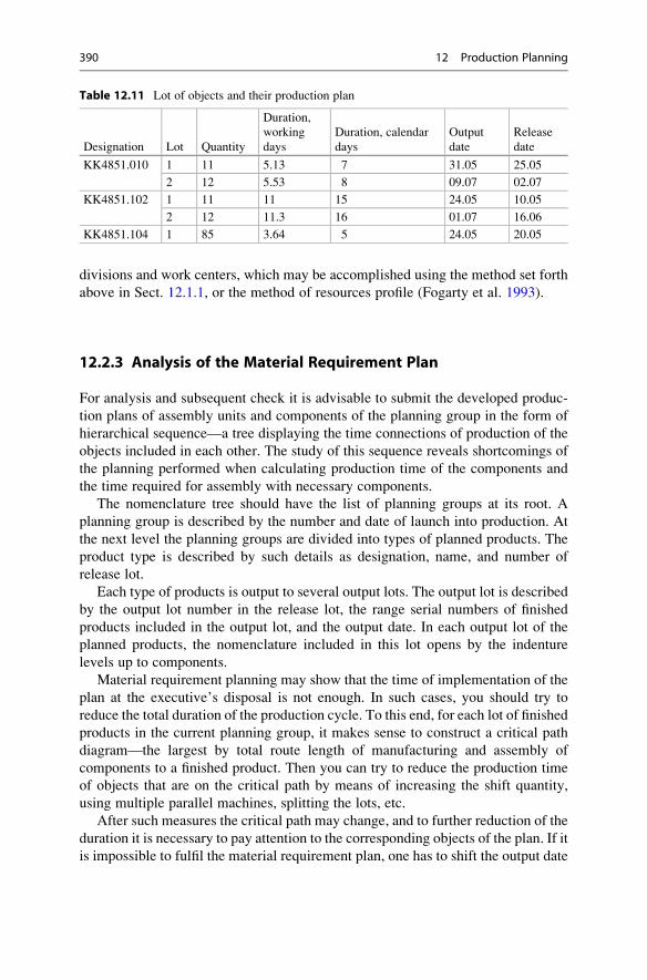
divisions and work centers, which may be accomplished using the method set forth
above in Sect. 12.1.1, or the method of resources profile (Fogarty et al. 1993).
12.2.3 Analysis of the Material Requirement Plan
For analysis and subsequent check it is advisable to submit the developed produc-
tion plans of assembly units and components of the planning group in the form of
hierarchical sequence—a tree displaying the time connections of production of the
objects included in each other. The study of this sequence reveals shortcomings of
the planning performed when calculating production time of the components and
the time required for assembly with necessary components.
The nomenclature tree should have the list of planning groups at its root. A
planning group is described by the number and date of launch into production. At
the next level the planning groups are divided into types of planned products. The
product type is described by such details as designation, name, and number of
release lot.
Each type of products is output to several output lots. The output lot is described
by the output lot number in the release lot, the range serial numbers of finished
products included in the output lot, and the output date. In each output lot of the
planned products, the nomenclature included in this lot opens by the indenture
levels up to components.
Material requirement planning may show that the time of implementation of the
plan at the executive’s disposal is not enough. In such cases, you should try to
reduce the total duration of the production cycle. To this end, for each lot of finished
products in the current planning group, it makes sense to construct a critical path
diagram—the largest by total route length of manufacturing and assembly of
components to a finished product. Then you can try to reduce the production time
of objects that are on the critical path by means of increasing the shift quantity,
using multiple parallel machines, splitting the lots, etc.
After such measures the critical path may change, and to further reduction of the
duration it is necessary to pay attention to the corresponding objects of the plan. If it
is impossible to fulfil the material requirement plan, one has to shift the output date
Table 12.11 Lot of objects and their production plan
Designation Lot Quantity
Duration,
working
days
Duration, calendar
days
Output
date
Release
date
KK4851.010 1 11 5.13 7 31.05 25.05
2 12 5.53 8 09.07 02.07
KK4851.102 1 11 11 15 24.05 10.05
2 12 11.3 16 01.07 16.06
KK4851.104 1 85 3.64 5 24.05 20.05
390 12 Production Planning
of the finished product in the master production plan. The issues of critical path
construction will be discussed in the next paragraph.
12.3 Project-Based Planning
A typical feature of project manufacturing is that it consists of a number of certain jobs,
and the execution of these jobs cannot be initiated before the completion of some others.
For these jobs, a network diagram is plotted that represents their relationship. The
network diagram is depicted as a direct graph—vertex set connected by directed arcs.
Network models distinguish the process of each job itself and the event asso-
ciated with its execution. The process is described by duration and the event of
execution determines the possibility of starting other jobs. Possible sequence of
jobs in the network model is a major constraint on their execution.
12.3.1 Critical Path Method
Let us consider set n of jobs required to complete the project. The execution of each of
these jobs may be defined by other job execution; in turn, the execution of each of the
jobsmay also be a prerequisite to start another job.We assume that the processing time
of each i-th job is known and equals pi. We also assume that the amount of equipment,
materials, finance, etc., is not limited, and set the least possible time to complete the
project, based only on the duration of the jobs.
At the initial instant that job can be executed, for which there are no constraints
on the sequence, and upon its completion the jobs can be performed, for which this
job is a constraint. To find the least possible time for project completion Cmax the
algorithm of “forward” planning is used, in which it is believed that the execution of
each possible job begins immediately after execution of the previous job. With this
algorithm the smallest possible time C0i for completion of the i-th job
C0i ¼ S0i þ pi; ð12:13Þ
where S0i is the least possible start time of the i-th job. It is obvious that the value
Cmax ¼ max C01;C
02; . . . ;C
0n
� : ð12:14Þ
Actually the start time of the i-th job is not necessarily equal to S0i. The job can be
started later than S0i, but provided that this delay will not influenceCmax. To calculate
these allowable delays, we use the “backward” planning which sets the largest
possible start time S0 0i of the i-th job.
12.3 Project-Based Planning 391
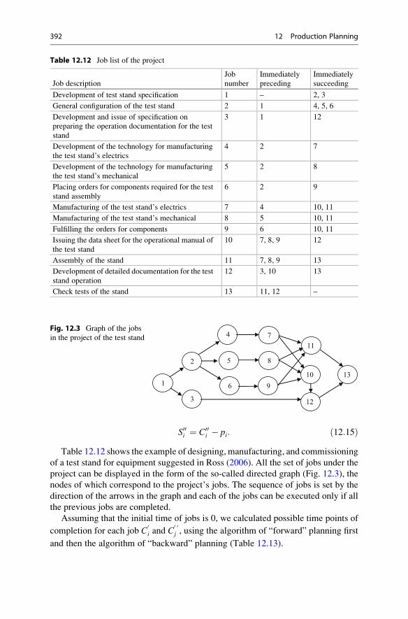
S00i ¼ C00i � pi: ð12:15Þ
Table 12.12 shows the example of designing, manufacturing, and commissioning
of a test stand for equipment suggested in Ross (2006). All the set of jobs under the
project can be displayed in the form of the so-called directed graph (Fig. 12.3), the
nodes of which correspond to the project’s jobs. The sequence of jobs is set by the
direction of the arrows in the graph and each of the jobs can be executed only if all
the previous jobs are completed.
Assuming that the initial time of jobs is 0, we calculated possible time points of
completion for each job C0i and C
0 0j , using the algorithm of “forward” planning first
and then the algorithm of “backward” planning (Table 12.13).
Table 12.12 Job list of the project
Job description
Job
number
Immediately
preceding
Immediately
succeeding
Development of test stand specification 1 – 2, 3
General configuration of the test stand 2 1 4, 5, 6
Development and issue of specification on
preparing the operation documentation for the test
stand
3 1 12
Development of the technology for manufacturing
the test stand’s electrics
4 2 7
Development of the technology for manufacturing
the test stand’s mechanical
5 2 8
Placing orders for components required for the test
stand assembly
6 2 9
Manufacturing of the test stand’s electrics 7 4 10, 11
Manufacturing of the test stand’s mechanical 8 5 10, 11
Fulfilling the orders for components 9 6 10, 11
Issuing the data sheet for the operational manual of
the test stand
10 7, 8, 9 12
Assembly of the stand 11 7, 8, 9 13
Development of detailed documentation for the test
stand operation
12 3, 10 13
Check tests of the stand 13 11, 12 –
1
2
3
4
5
6
7
8
9
11
10
12
13
Fig. 12.3 Graph of the jobs
in the project of the test stand
392 12 Production Planning
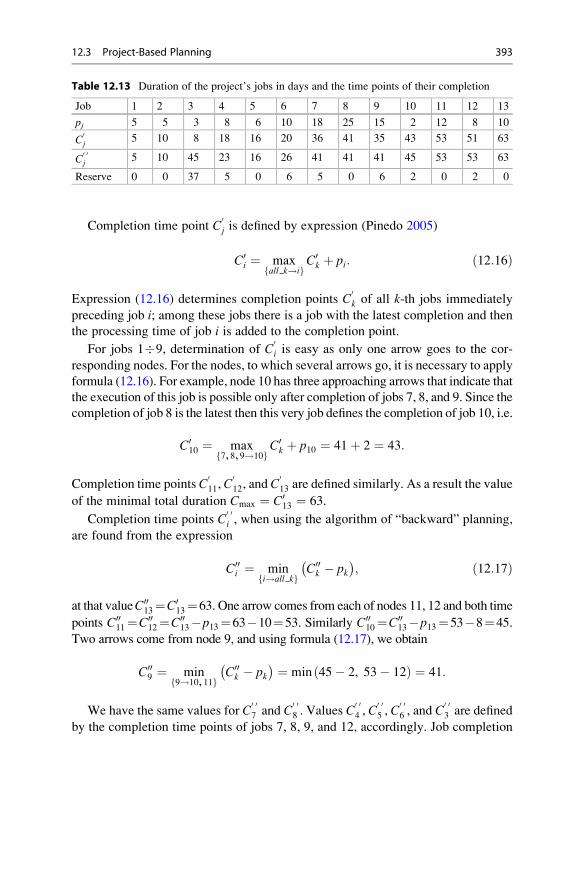
Completion time point C0j is defined by expression (Pinedo 2005)
C0i ¼ max
all k!if gC0k þ pi: ð12:16Þ
Expression (12.16) determines completion points C0k of all k-th jobs immediately
preceding job i; among these jobs there is a job with the latest completion and then
the processing time of job i is added to the completion point.
For jobs 1�9, determination of C0i is easy as only one arrow goes to the cor-
responding nodes. For the nodes, to which several arrows go, it is necessary to apply
formula (12.16). For example, node 10 has three approaching arrows that indicate that
the execution of this job is possible only after completion of jobs 7, 8, and 9. Since the
completion of job 8 is the latest then this very job defines the completion of job 10, i.e.
C010 ¼ max
7, 8, 9!10f gC0k þ p10 ¼ 41þ 2 ¼ 43:
Completion time points C011, C
012, and C
013 are defined similarly. As a result the value
of the minimal total duration Cmax ¼ C013 ¼ 63.
Completion time points C0 0i , when using the algorithm of “backward” planning,
are found from the expression
C00i ¼ min
i!all kf gC00k � pk
� ; ð12:17Þ
at that valueC0013¼C0
13¼63. One arrow comes from each of nodes 11, 12 and both time
points C0011¼C00
12¼C0013�p13¼63�10¼53. Similarly C00
10¼C0013�p13¼53�8¼45.
Two arrows come from node 9, and using formula (12.17), we obtain
C009 ¼ min
9!10, 11f gC00k � pk
� ¼ min 45� 2, 53� 12ð Þ ¼ 41:
We have the same values for C0 07 and C
0 08 . Values C
0 04 , C
0 05 , C
0 06 , and C
0 03 are defined
by the completion time points of jobs 7, 8, 9, and 12, accordingly. Job completion
Table 12.13 Duration of the project’s jobs in days and the time points of their completion
Job 1 2 3 4 5 6 7 8 9 10 11 12 13
pj 5 5 3 8 6 10 18 25 15 2 12 8 10
C0j
5 10 8 18 16 20 36 41 35 43 53 51 63
C0 0j
5 10 45 23 16 26 41 41 41 45 53 53 63
Reserve 0 0 37 5 0 6 5 0 6 2 0 2 0
12.3 Project-Based Planning 393
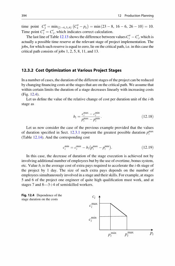
time point C002 ¼ min 2!4, 5, 6f g C00
k � pk� ¼ min 23� 8, 16� 6, 26� 10ð Þ ¼ 10.
Time point C001 ¼ C0
1, which indicates correct calculation.
The last line of Table 12.13 shows the difference between valuesC00i � C0
i, which is
actually a possible time reserve at the relevant stage of project implementation. The
jobs, for which such reserve is equal to zero, lie on the critical path, i.e. in this case the
critical path consists of jobs 1, 2, 5, 8, 11, and 13.
12.3.2 Cost Optimization at Various Project Stages
In a number of cases, the duration of the different stages of the project can be reduced
by changing financing costs at the stages that are on the critical path.We assume that
within certain limits the duration of a stage decreases linearly with increasing costs
(Fig. 12.4).
Let us define the value of the relative change of cost per duration unit of the i-thstage as
bi ¼ cmaxi � cmin
i
pmaxi � pmin
i
: ð12:18Þ
Let us now consider the case of the previous example provided that the values
of duration specified in Sect. 12.3.1 represent the greatest possible duration pmaxi
(Table 12.14). And the corresponding cost
cmini ¼ cmax
i � bi pmaxi � pmin
i
� : ð12:19Þ
In this case, the decrease of duration of the stage execution is achieved not by
involving additional number of employees but by the use of overtime, bonus system,
etc. Value bi is the average cost of extra pays required to accelerate the i-th stage ofthe project by 1 day. The size of such extra pays depends on the number of
employees simultaneously involved in a stage and their skills. For example, at stages
5 and 6 of the project one engineer of quite high qualification must work, and at
stages 7 and 8—3�4 of semiskilled workers.
ipminip max
ip
icmaxic
minic
Fig. 12.4 Dependence of the
stage duration on the costs
394 12 Production Planning
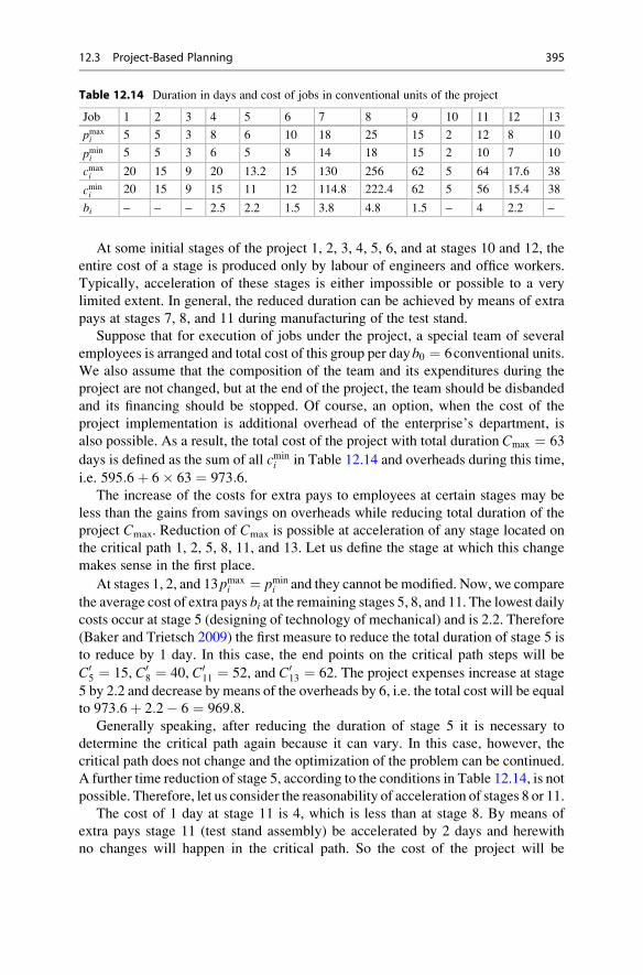
At some initial stages of the project 1, 2, 3, 4, 5, 6, and at stages 10 and 12, the
entire cost of a stage is produced only by labour of engineers and office workers.
Typically, acceleration of these stages is either impossible or possible to a very
limited extent. In general, the reduced duration can be achieved by means of extra
pays at stages 7, 8, and 11 during manufacturing of the test stand.
Suppose that for execution of jobs under the project, a special team of several
employees is arranged and total cost of this group per dayb0 ¼ 6conventional units.
We also assume that the composition of the team and its expenditures during the
project are not changed, but at the end of the project, the team should be disbanded
and its financing should be stopped. Of course, an option, when the cost of the
project implementation is additional overhead of the enterprise’s department, is
also possible. As a result, the total cost of the project with total duration Cmax ¼ 63
days is defined as the sum of all cmini in Table 12.14 and overheads during this time,
i.e. 595:6þ 6� 63 ¼ 973:6.The increase of the costs for extra pays to employees at certain stages may be
less than the gains from savings on overheads while reducing total duration of the
project Cmax. Reduction of Cmax is possible at acceleration of any stage located on
the critical path 1, 2, 5, 8, 11, and 13. Let us define the stage at which this change
makes sense in the first place.
At stages 1, 2, and 13pmaxi ¼ pmin
i and they cannot be modified. Now, we compare
the average cost of extra pays bi at the remaining stages 5, 8, and 11. The lowest daily
costs occur at stage 5 (designing of technology of mechanical) and is 2.2. Therefore
(Baker and Trietsch 2009) the first measure to reduce the total duration of stage 5 is
to reduce by 1 day. In this case, the end points on the critical path steps will be
C05 ¼ 15, C0
8 ¼ 40, C011 ¼ 52, and C0
13 ¼ 62. The project expenses increase at stage
5 by 2.2 and decrease by means of the overheads by 6, i.e. the total cost will be equal
to 973:6þ 2:2� 6 ¼ 969:8.Generally speaking, after reducing the duration of stage 5 it is necessary to
determine the critical path again because it can vary. In this case, however, the
critical path does not change and the optimization of the problem can be continued.
A further time reduction of stage 5, according to the conditions in Table 12.14, is not
possible. Therefore, let us consider the reasonability of acceleration of stages 8 or 11.
The cost of 1 day at stage 11 is 4, which is less than at stage 8. By means of
extra pays stage 11 (test stand assembly) be accelerated by 2 days and herewith
no changes will happen in the critical path. So the cost of the project will be
Table 12.14 Duration in days and cost of jobs in conventional units of the project
Job 1 2 3 4 5 6 7 8 9 10 11 12 13
pmaxi 5 5 3 8 6 10 18 25 15 2 12 8 10
pmini
5 5 3 6 5 8 14 18 15 2 10 7 10
cmaxi 20 15 9 20 13.2 15 130 256 62 5 64 17.6 38
cmini
20 15 9 15 11 12 114.8 222.4 62 5 56 15.4 38
bi – – – 2.5 2.2 1.5 3.8 4.8 1.5 – 4 2.2 –
12.3 Project-Based Planning 395
969:8þ 2945:44� 2� 6 ¼ 945:4 and the completion time points of the stages on
the critical path will be C011 ¼ 50 and C0
13 ¼ 60.
The further acceleration can be achieved only bymeans of stage 8 (manufacturing
of mechanical part). According to Table 12.14 the duration of stage 8 can be reduced
from 25 to 18 days. If we reduce the duration gradually by 1 day, then the critical
path set earlier will remain up to the third days inclusive, and on the fourth day the
duration of path 1, 2, 5, 8, 11, and 13 will be equal to the duration of path 1, 2, 4, 7,
11, and 13 (Fig. 12.3). On the fourth day of the reduction of stage 8 we obtain the
total cost of the project 945:4þ 4� 4:8� 4� 6 ¼ 940:6.Now, to further reduce the duration it is necessary to compare values bi for stage
8 on critical path 1, 2, 5, 8, 11, 13, and stages 4 and 7 on critical path 1, 2, 4, 7,
11, 13. The least one is obviously value b4 ¼ 2:5, and the duration of stage 4 shouldbe reduced by 1 day. However, after acceleration of stage 4, path 1, 2, 5, 8, 11, 13
will become critical again, whereby the duration of stage 8 should undergo reduc-
tion. As a result the completion time points will beC04 ¼ 17,C0
7 ¼ 35, andC08 ¼ 35.
From Fig. 12.3 and Table 12.13, it follows that in this situation there are three
critical paths at the same time: 1, 2, 5, 8, 11, 13; 1, 2, 4, 7, 11, 13; and 1, 2, 6, 9,
11, 13.
Obviously, further reducing of the project duration is only possible if it is possible
on all three critical paths simultaneously. In this case, in the first of the paths the
duration of stage 4 can be reduced, in the second—stage 4, and the third—stage
6. Thereafter, a new critical path 1, 2, 6, 9, 10, 12, 13 appears. Since, however,
opportunity to accelerate stage 4 is exhausted, the further process terminates. The
result is shown in Table 12.15.
In Table 12.15 pi is the accepted planned duration in days and ci is the plannedcost of the stage in conventional units. As can be seen from Table 12.15, as a result
of optimization stages 4, 5, 6, 8, and 11 underwent acceleration, so the total duration
decreased from 63 to 54 days, and the time reserves at the most of stages appeared
to be zero. Herewith the total cost of the project isXciþ b0 � Cmax ¼ 641þ 6� 54 ¼ 965:
The considered problem can be solved by linear programming methods. To do
this, we have to find the minimum of expression (Pinedo 2005)
b0 � Cmax �Xni¼1
bipi ð12:20Þ
with constraints:
xk � pi � xi � 0 forall i ! k and xi � 0; ð12:21Þ
pi � pmaxi and pi � pmin
i forall i; ð12:22Þ
396 12 Production Planning
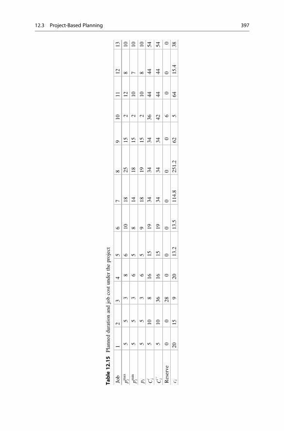
Table
12.15
Planned
durationandjobcostunder
theproject
Job
12
34
56
78
910
11
12
13
pmax
i5
53
86
10
18
25
15
212
810
pmin
i5
53
65
814
18
15
210
710
pi
55
36
59
18
19
15
210
810
C0 i
510
816
15
19
34
34
34
36
44
44
54
C00 i
510
36
16
15
19
34
34
34
42
44
44
54
Reserve
00
28
00
00
00
60
00
c i20
15
920
13.2
13.5
114.8
251.2
62
564
15.4
38
12.3 Project-Based Planning 397

Cmax � xi � pi � 0: ð12:23ÞIn expressions (12.21), values xi are variable time points of beginning of each
project stage. The independent variables of the problem are pi, xi, and Cmax. In
particular in this example with 13 jobs, the number of variables is13þ 13þ 1 ¼ 27.
The number of constraints (12.21) is equal to the number of the graph arcs (arrows)
in Fig. 12.3, i.e. in this case 18.
The solution of problem (12.20–12.23) exists if at least some of extra pays cost
values bi on the critical path, which ensure the acceleration of the stage by 1 day, areless than the daily overhead b0. Otherwise, any attempt to reduce the process time
will be associated with an increase in total costs, and the problem becomes multi-
objective. Such a problem can also be solved, but with the help of methods of the
theory of utility and decision-making outlined above in Chap. 4.
12.4 Stability of Planning
The stability of planning has influence on all aspects of the enterprise activity quite
remarkably, but, of course, primarily on the production process. The reasons of changes
in the developed plans can be divided into primary (independent) and secondary, which
are derived from the primary reasons. If we consider the planning and production
processes as a single system, it is necessary to consider that it operates in the context of
regular exposure to a variety of disturbances that prevent accomplishing the objectives
of the system (Fig. 12.5).
In Fig. 12.5 the bold arrows indicate the planned material and information flows
in the system, and the thin solid arrows—the disturbances. These disturbances cause
changes in the plans, which are automatically transmitted to downstream echelons of
the system. If these echelons have reserves sufficient to respond to the disturbances
obtained, the information about such disturbances is not transmitted to the echelons
of higher level.
Internal reserves of the system, as it follows from Fig. 12.5, consist of time buffer
between the material requirement and operations plan and buffer stocks of interme-
diate products and finished products. If the reserve is not enough, then, as shown by
the dashed arrows, the information about the current situation can be transmitted
to the next superior level with the request or suggestion of changes in the relevant
plans.
Thus, the stability of planning is determined by two groups of factors: (a) external
influences and (b) internal reserves. The external factors are random and it is generally
believed that their value has a normal distribution. It is obvious that the volumes of
internal reserves should be set essentially depending on the amplitude and dispersion
of possible changes.
The unstable planning affects the productivity greatly. For example, the study
(Pujawan 2004) carried out in the shoe industry showed that the actual changes in
the plans of various levels reduce the production output on the shop level by 20 %
on average.
398 12 Production Planning
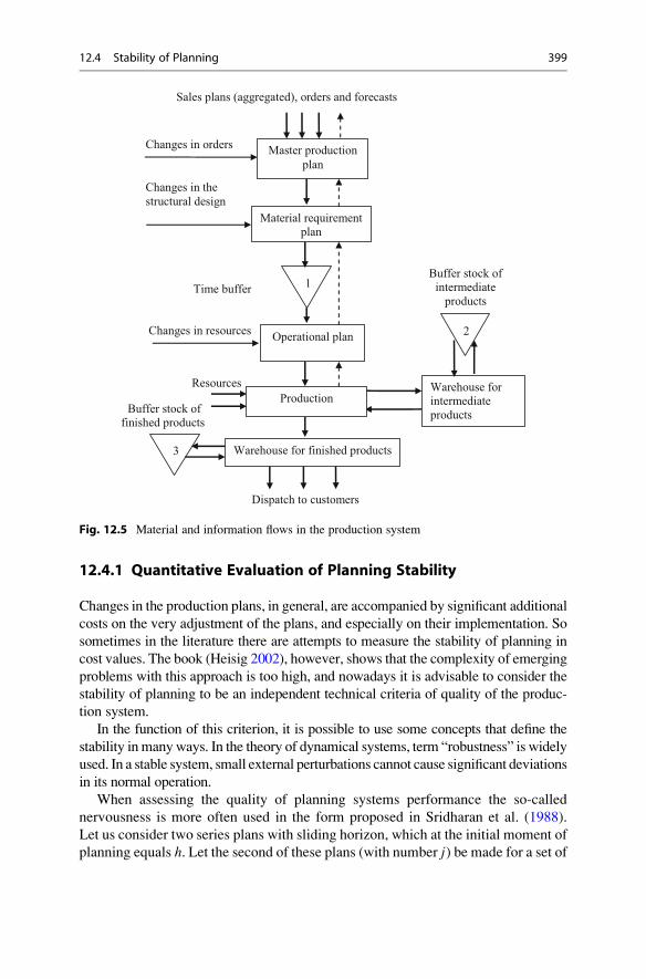
12.4.1 Quantitative Evaluation of Planning Stability
Changes in the production plans, in general, are accompanied by significant additional
costs on the very adjustment of the plans, and especially on their implementation. So
sometimes in the literature there are attempts to measure the stability of planning in
cost values. The book (Heisig 2002), however, shows that the complexity of emerging
problems with this approach is too high, and nowadays it is advisable to consider the
stability of planning to be an independent technical criteria of quality of the produc-
tion system.
In the function of this criterion, it is possible to use some concepts that define the
stability in manyways. In the theory of dynamical systems, term “robustness” is widely
used. In a stable system, small external perturbations cannot cause significant deviations
in its normal operation.
When assessing the quality of planning systems performance the so-called
nervousness is more often used in the form proposed in Sridharan et al. (1988).
Let us consider two series plans with sliding horizon, which at the initial moment of
planning equals h. Let the second of these plans (with number j) be made for a set of
Buffer stock of intermediate
products
Buffer stock of finished products
Resources
Changes in the structural design
Master production
plan
Material requirement plan
1
Operational plan
3
2
Warehouse for intermediate products
Production
Warehouse for finished products
Sales plans (aggregated), orders and forecasts
Dispatch to customers
Changes in orders
Changes in resources
Time buffer
Fig. 12.5 Material and information flows in the production system
12.4 Stability of Planning 399
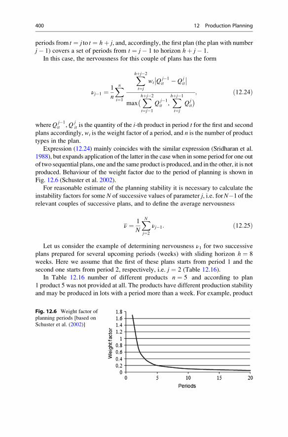
periods from t ¼ j to t ¼ hþ j, and, accordingly, the first plan (the plan with number
j� 1) covers a set of periods from t ¼ j� 1 to horizon hþ j� 1.
In this case, the nervousness for this couple of plans has the form
νj�1 ¼ 1
n
Xni¼1
Xhþj�2
t¼j
wt
��Q j�1it � Qj
it
��max
�Xhþj�2
t¼j�1
Q j�1it ,
Xhþj�1
t¼j
Q jit
; ð12:24Þ
whereQ j�1it , Q j
it is the quantity of the i-th product in period t for the first and secondplans accordingly, wt is the weight factor of a period, and n is the number of product
types in the plan.
Expression (12.24) mainly coincides with the similar expression (Sridharan et al.
1988), but expands application of the latter in the case when in some period for one out
of two sequential plans, one and the same product is produced, and in the other, it is not
produced. Behaviour of the weight factor due to the period of planning is shown in
Fig. 12.6 (Schuster et al. 2002).
For reasonable estimate of the planning stability it is necessary to calculate the
instability factors for some N of successive values of parameter j, i.e. forN�1of the
relevant couples of successive plans, and to define the average nervousness
ν ¼ 1
N
XNj¼2
νj�1: ð12:25Þ
Let us consider the example of determining nervousness ν1 for two successive
plans prepared for several upcoming periods (weeks) with sliding horizon h ¼ 8
weeks. Here we assume that the first of these plans starts from period 1 and the
second one starts from period 2, respectively, i.e. j ¼ 2 (Table 12.16).
In Table 12.16 number of different products n ¼ 5 and according to plan
1 product 5 was not provided at all. The products have different production stability
and may be produced in lots with a period more than a week. For example, product
Fig. 12.6 Weight factor of
planning periods [based on
Schuster et al. (2002)]
400 12 Production Planning
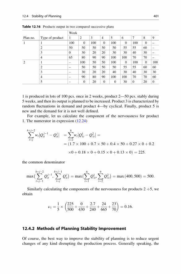
1 is produced in lots of 100 pcs. once in 2 weeks, product 2—50 pcs. stably during
5 weeks, and then its output is planned to be increased. Product 3 is characterized by
random fluctuations in demand and product 4—by cyclical. Finally, product 5 is
new and the demand for it is not well defined.
For example, let us calculate the component of the nervousness for product
1. The numerator in expression (12.24)
Xhþj�2
t¼j
wt
��Q j�1it � Qj
it
�� ¼X8t¼2
wt
��Q11t � Q2
1t
�� ¼¼ 1:7� 100þ 0:7� 50þ 0:4� 50þ 0:27� 0þ 0:2ð
�0þ 0:18� 0þ 0:15� 0þ 0:13� 0Þ ¼ 225:
the common denominator
max�Xhþj�2
t¼j�1
Qj�1it ,
Xhþj�1
t¼j
Q jit
¼ max�X8t¼1
Q11t,X9t¼2
Q21t
¼ max 400; 500ð Þ ¼ 500:
Similarly calculating the components of the nervousness for products 2 �5, we
obtain
ν1 ¼ 1
5� 225
500þ 0
430þ 2:7
240þ 24
665þ 23
70
� �¼ 0:16:
12.4.2 Methods of Planning Stability Improvement
Of course, the best way to improve the stability of planning is to reduce urgent
changes of any kind disrupting the production process. Generally speaking, the
Table 12.16 Products output in two compared successive plans
Plan no. Type of product
Week
1 2 3 4 5 6 7 8 9
1 1 100 0 100 0 100 0 100 0 –
2 50 50 50 50 50 55 55 60 –
3 0 30 20 20 30 30 40 30 –
4 65 80 90 90 100 100 70 70 –
2 1 – 100 50 50 100 0 100 0 100
2 – 50 50 50 50 55 55 60 60
3 – 30 20 20 40 30 40 30 30
4 – 90 80 90 100 100 70 70 60
5 – 0 20 0 0 30 0 20 0
12.4 Stability of Planning 401

changes in the long-term plans are inevitable and even useful because they reflect
the scientific, technological, and social progress. Urgent changes occur in the result
of either force majeure or unreasoned decisions, and, for the most part, the latter
occurs more often.
Virtually all of the ways to enhance the stability of planning are aimed at damping
of disturbance due to urgent changes. There are basically five ways to enhance the
stability:
• “Freezing” some part of the master plan;
• Provision of sufficient buffer sizes;
• Efficient sizing of lots;
• Prevention of urgent changes;
• Using of substitutes.
The plan “freezing” consists in abandoning changes to that part of the current
plan, implementation of which has already passed the stage of pre-production and
blanking operation. In such cases, the production process is usually irreversible
already and attempts to introduce changes often lead to the production breakdown.
Of course, such freezing has a negative side, because unnecessary or substandard
products might be produced. Furthermore, freezing is physically impossible in the
event of some resource shortage.
It is natural to use the freezing in group planning. In this case, it makes sense to
freeze the plans of components lots launching, because freezing is carried out either
after the blanking operations or in process of their performance. At the same time,
the plans of output lots of components and assembly units may not be frozen but
adjusted. Using the planning group, consisting of both external and internal orders,
allows manoeuvring when resizing and even changing of orders due dates by means
of transferring some part of products from the external to the internal order and vice
versa.
Time buffer 1 in Fig. 12.5 provides some time reserves for workshops, which can
be used to adjust operational plans. The availability ofmaterial buffers 2 and 3 allows
to provide a continuous production process in case of the delays associated with
changes in resources.
Reasonable buffer sizing is the main way to maintain stable operation of the pro-
duction system. To do this, it is advisable to calculate average nervousness of
planning ν regularly by the method described in the above paragraph and determine
its dependence on the buffer sizes empirically.
In some cases, the plans stability can be improved with proper lot sizing or
orders. In the paper (Heisig 2002) the detailed study of the planning stability in the
supply chain for the model with fixed order quantity (Sect. 8.2.1) and the two-level
model (Sect. 8.2.3) for randomly changing demand was carried out.
Figure 12.7 shows the estimated dependence of panning stability value 1� ν on
relative lot sizeQ/D, based on the results in (Heisig 2002), whereD is the demand per
base forecasting period. As can be seen from Fig. 12.7, in the range of 1 � Q=D � 3
the sharp decrease in the planning stability can be observed. Based on these data, the
402 12 Production Planning
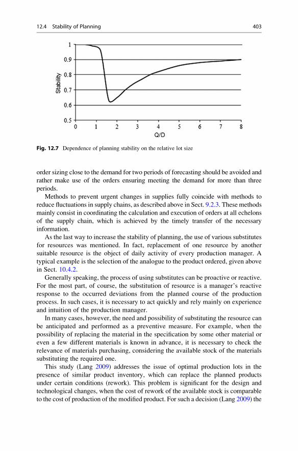
order sizing close to the demand for two periods of forecasting should be avoided and
rather make use of the orders ensuring meeting the demand for more than three
periods.
Methods to prevent urgent changes in supplies fully coincide with methods to
reduce fluctuations in supply chains, as described above in Sect. 9.2.3. These methods
mainly consist in coordinating the calculation and execution of orders at all echelons
of the supply chain, which is achieved by the timely transfer of the necessary
information.
As the last way to increase the stability of planning, the use of various substitutes
for resources was mentioned. In fact, replacement of one resource by another
suitable resource is the object of daily activity of every production manager. A
typical example is the selection of the analogue to the product ordered, given above
in Sect. 10.4.2.
Generally speaking, the process of using substitutes can be proactive or reactive.
For the most part, of course, the substitution of resource is a manager’s reactive
response to the occurred deviations from the planned course of the production
process. In such cases, it is necessary to act quickly and rely mainly on experience
and intuition of the production manager.
In many cases, however, the need and possibility of substituting the resource can
be anticipated and performed as a preventive measure. For example, when the
possibility of replacing the material in the specification by some other material or
even a few different materials is known in advance, it is necessary to check the
relevance of materials purchasing, considering the available stock of the materials
substituting the required one.
This study (Lang 2009) addresses the issue of optimal production lots in the
presence of similar product inventory, which can replace the planned products
under certain conditions (rework). This problem is significant for the design and
technological changes, when the cost of rework of the available stock is comparable
to the cost of production of the modified product. For such a decision (Lang 2009) the
Fig. 12.7 Dependence of planning stability on the relative lot size
12.4 Stability of Planning 403
statements of the problems, described above in Sects. 11.1.2–11.1.4, are used for
optimal lot sizes in the presence of constraints; for this purpose the objective functions
take into account the rework cost of the product substituting the planned one.
References
Baker, K. R., & Trietsch, D. (2009). Principles of sequencing and scheduling. New York: Wiley.
Chung, C., & Krajevski, L. J. (1984). Planning horizons for master production scheduling. Journalof Operations Management, 8, 389–406.
Fogarty, D. W., Blackstone, J. H., & Hoffmann, T. R. (1993). Production and inventory manage-ment. Cincinnati, OH: South-Western Publishing Co.
Heisig, G. (2002). Planning stability in material requirements planning systems. Berlin: Springer.Lang, J. C. (2009). Production and inventory management with substitutions. Heidelberg:
Springer.
Mauergauz, Y. (2007). Computer aided operative planning in mechanical engineering. Moscow:
Economics (in Russian).
Pinedo, M. L. (2005). Planning and scheduling in manufacturing and services. Berlin: Springer.Pujawan, I. N. (2004). Schedule nervousness in a manufacturing system: a case study. Production
Planning and Control, 15, 515–524.Ross, S. I. (2006). Mathematical modelling and study of nation economy. Saint-Petersburg:
SPbGU ITMO (in Russian).
Sachko, N. S. (2008). Organization and operational management of machinery production.Minsk: Novoe znaniye (in Russian).
Schuster, E. W., Unahabhokha, C., & Allen, S. J. (2002). Master production schedule stabilityunder conditions of finite capacity. mit.edu/edmund_w/www/LEC20054-14-05R1.pdf.
Shapiro, J. F. (2001). Modelling the supply chain. Pacific Grove, CA: Thomson Learning.
Sridharan, S. V., Berry, W. L., & Udayabhanu, V. (1988). Measuring master production schedule
stability under rolling planning horizons. Decision Sciences, 19, 147–166.Vollmann, T. E., Berry, W. L., Whybark, D. C., & Jacobs, F. R. (2005). Manufacturing planning
and control for supply chain management. Boston: McGraw Hill.
404 12 Production Planning
Shop Floor Scheduling: Single-StageProblems 13
13.1 Single-Machine Scheduling with Minimized OverduePenalties
The problem of planning is called single stage, if every job can be fully executed on
one of the available machines. In the simplest case, the production system consists
of a single machine, on which all planned jobs can be performed. The schedule for
such a machine is a sequence of execution of the jobs already received, as well as
the jobs that may arrive in the near future.
An elementary or basic version of the problem is based on the following seven
assumptions:
(a) All of the planned jobs are equally available at the beginning of the planning.
(b) Only one work is simultaneously executed.
(c) Machine setup time does not depend on the order of execution of jobs and is
included in the duration of this job.
(d) Duration of each job is determined and known.
(e) The machine is available and serviceable at any time.
(f) Machine idle time is not allowed if there is a job to be performed.
(g) Each job is executed to the end without interruption for another job.
In accordance with the classification (2.13) above in Sect. 2.2.2, in different
cases of scheduling for a single machine the problem formula has the form
1��β��γ; ð13:1Þ
where the constraints of various types are recorded in field β. They are superimposed on
the dates of job start and end. The designation of the objective function is recorded in
field γ. To optimize the schedule of the machine in the described variant of organiza-
tion, various criteria, described in Sect. 2.2.2, can be used, except for makespan Cmax,
# Springer International Publishing Switzerland 2016
Y. Mauergauz, Advanced Planning and Scheduling in Manufacturing and SupplyChains, DOI 10.1007/978-3-319-27523-9_13
405
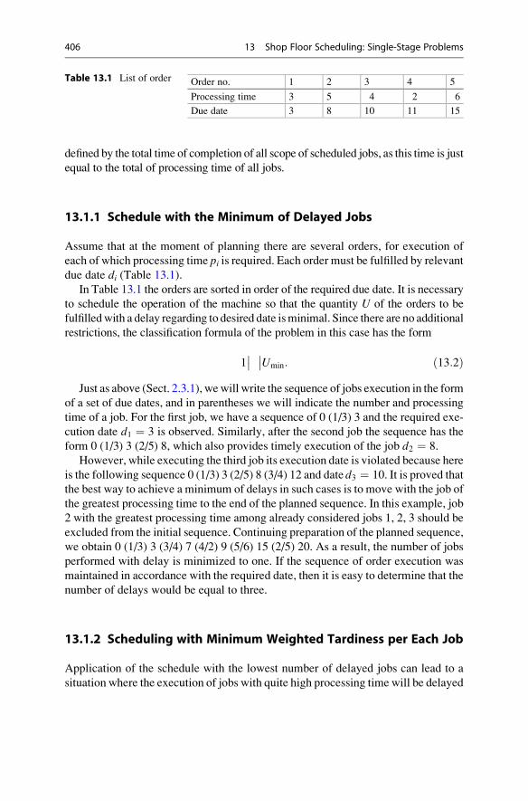
defined by the total time of completion of all scope of scheduled jobs, as this time is just
equal to the total of processing time of all jobs.
13.1.1 Schedule with the Minimum of Delayed Jobs
Assume that at the moment of planning there are several orders, for execution of
each of which processing time pi is required. Each order must be fulfilled by relevant
due date di (Table 13.1).In Table 13.1 the orders are sorted in order of the required due date. It is necessary
to schedule the operation of the machine so that the quantity U of the orders to be
fulfilledwith a delay regarding to desired date isminimal. Since there are no additional
restrictions, the classification formula of the problem in this case has the form
1�� ��Umin: ð13:2Þ
Just as above (Sect. 2.3.1), wewill write the sequence of jobs execution in the form
of a set of due dates, and in parentheses we will indicate the number and processing
time of a job. For the first job, we have a sequence of 0 (1/3) 3 and the required exe-
cution date d1 ¼ 3 is observed. Similarly, after the second job the sequence has the
form 0 (1/3) 3 (2/5) 8, which also provides timely execution of the job d2 ¼ 8.
However, while executing the third job its execution date is violated because here
is the following sequence 0 (1/3) 3 (2/5) 8 (3/4) 12 and dated3 ¼ 10. It is proved that
the best way to achieve a minimum of delays in such cases is to move with the job of
the greatest processing time to the end of the planned sequence. In this example, job
2 with the greatest processing time among already considered jobs 1, 2, 3 should be
excluded from the initial sequence. Continuing preparation of the planned sequence,
we obtain 0 (1/3) 3 (3/4) 7 (4/2) 9 (5/6) 15 (2/5) 20. As a result, the number of jobs
performed with delay is minimized to one. If the sequence of order execution was
maintained in accordance with the required date, then it is easy to determine that the
number of delays would be equal to three.
13.1.2 Scheduling with Minimum Weighted Tardiness per Each Job
Application of the schedule with the lowest number of delayed jobs can lead to a
situation where the execution of jobs with quite high processing time will be delayed
Table 13.1 List of order Order no. 1 2 3 4 5
Processing time 3 5 4 2 6
Due date 3 8 10 11 15
406 13 Shop Floor Scheduling: Single-Stage Problems
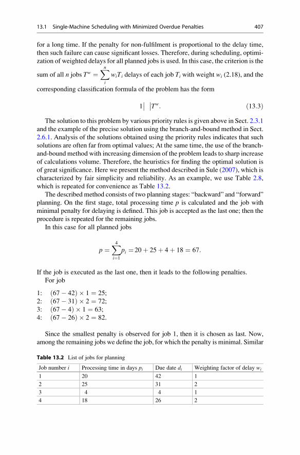
for a long time. If the penalty for non-fulfilment is proportional to the delay time,
then such failure can cause significant losses. Therefore, during scheduling, optimi-
zation of weighted delays for all planned jobs is used. In this case, the criterion is the
sum of all n jobs Tw ¼Xni
wiTi delays of each job Ti with weight wi (2.18), and the
corresponding classification formula of the problem has the form
1�� ��Tw: ð13:3Þ
The solution to this problem by various priority rules is given above in Sect. 2.3.1
and the example of the precise solution using the branch-and-bound method in Sect.
2.6.1. Analysis of the solutions obtained using the priority rules indicates that such
solutions are often far from optimal values; At the same time, the use of the branch-
and-bound method with increasing dimension of the problem leads to sharp increase
of calculations volume. Therefore, the heuristics for finding the optimal solution is
of great significance. Here we present the method described in Sule (2007), which is
characterized by fair simplicity and reliability. As an example, we use Table 2.8,
which is repeated for convenience as Table 13.2.
The described method consists of two planning stages: “backward” and “forward”
planning. On the first stage, total processing time p is calculated and the job with
minimal penalty for delaying is defined. This job is accepted as the last one; then the
procedure is repeated for the remaining jobs.
In this case for all planned jobs
p ¼X4i¼1
pi ¼ 20þ 25þ 4þ 18 ¼ 67:
If the job is executed as the last one, then it leads to the following penalties.
For job
1: 67� 42ð Þ � 1 ¼ 25;
2: 67� 31ð Þ � 2 ¼ 72;
3: 67� 4ð Þ � 1 ¼ 63;
4: 67� 26ð Þ � 2 ¼ 82.
Since the smallest penalty is observed for job 1, then it is chosen as last. Now,
among the remaining jobs we define the job, for which the penalty is minimal. Similar
Table 13.2 List of jobs for planning
Job number i Processing time in days pi Due date di Weighting factor of delay wi
1 20 42 1
2 25 31 2
3 4 4 1
4 18 26 2
13.1 Single-Machine Scheduling with Minimized Overdue Penalties 407
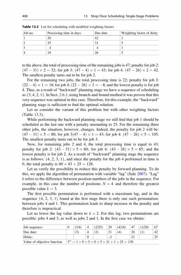
to the above, the total of processing time of the remaining jobs is 47; penalty for job 2:
47� 31ð Þ � 2 ¼ 32; for job 3: 47� 4ð Þ � 1 ¼ 43; for job 4: 47� 26ð Þ � 2 ¼ 42.
The smallest penalty turns out to be for job 2.
For the remaining two jobs, the total processing time is 22; penalty for job 3:
22� 4ð Þ � 1 ¼ 18; for job 4: 22� 26ð Þ � 2 ¼ �8; and the lowest penalty is for job
4. Thus, as a result of “backward” planning stage we have a sequence of scheduling
as {3, 4, 2, 1}. In Sect. 2.6.1, using branch-and-bound method it was proven that this
very sequence was optimal in this case. Therefore, for this example, the “backward”
planning stage is sufficient to find the optimal solution.
Let us consider the variant of this problem but with other weighting factors
(Table 13.3).
While performing the backward planning stage we still find that job 1 should be
scheduled as the last one with a penalty amounting to 25. For the remaining three
other jobs, the situation, however, changes. Indeed, the penalty for job 2 will be:
47� 31ð Þ � 5 ¼ 80; for job 3 47� 4ð Þ � 1 ¼ 43; for job 4: 47� 26ð Þ � 5 ¼ 105.
The smallest penalty turns out to be for job 3.
Now, for remaining jobs 2 and 4, the total processing time is equal to 43;
penalty for job 2: 43� 31ð Þ � 5 ¼ 60; for job 4: 43� 26ð Þ � 5 ¼ 85; and the
lowest penalty is for job 2. As a result of “backward” planning stage the sequence
is as follows: {4, 2, 3, 1}, and since the penalty for the job 4 performed in time is
0, the total penalty is 60þ 43þ 25 ¼ 128.
Let us verify the possibility to reduce this penalty by forward planning. To do
this, we apply the algorithm of permutation with variable “lag” (Sule 2007). “Lag”
k refers to the difference between position numbers of the jobs in the sequence. For
example, in this case the number of positions N ¼ 4 and therefore the greatest
possible value k ¼ 3.
The first possible permutation is performed with a maximum lag, and in the
sequence {4, 2, 3, 1} found at the first stage there is only one such permutation:
between jobs 4 and 1. This permutation leads to sharp increase in the penalty and
therefore is impractical.
Let us lower the lag value down to k ¼ 2. For this lag, two permutations are
possible: jobs 4 and 3, as well as jobs 2 and 1. In the first case we obtain:
Job sequence: 0 (3/4) 4 (2/25) 29 (4/18) 47 (1/20) 67
Due date: (3) 4 (2) 31 (4) 26 (1) 42
Delay: 0 –2 21 25
Value of objective function Tw ¼ 1� 0þ 5� 0þ 5� 21þ 1� 25 ¼ 130:
Table 13.3 List for scheduling with modified weighting factors
Job no. Processing time in days Due date Weighting factor of delay
1 20 42 1
2 25 31 5
3 4 4 1
4 18 26 5
408 13 Shop Floor Scheduling: Single-Stage Problems
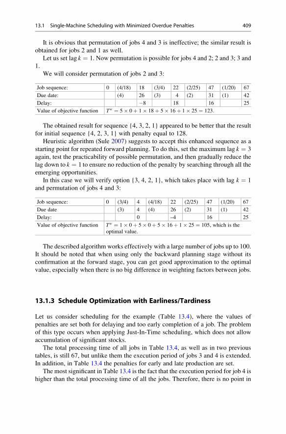
It is obvious that permutation of jobs 4 and 3 is ineffective; the similar result is
obtained for jobs 2 and 1 as well.
Let us set lag k ¼ 1. Now permutation is possible for jobs 4 and 2; 2 and 3; 3 and
1.
We will consider permutation of jobs 2 and 3:
Job sequence: 0 (4/18) 18 (3/4) 22 (2/25) 47 (1/20) 67
Due date: (4) 26 (3) 4 (2) 31 (1) 42
Delay: �8 18 16 25
Value of objective function Tw ¼ 5� 0þ 1� 18þ 5� 16þ 1� 25 ¼ 123:
The obtained result for sequence {4, 3, 2, 1} appeared to be better that the result
for initial sequence {4, 2, 3, 1} with penalty equal to 128.
Heuristic algorithm (Sule 2007) suggests to accept this enhanced sequence as a
starting point for repeated forward planning. To do this, set the maximum lag k ¼ 3
again, test the practicability of possible permutation, and then gradually reduce the
lag down to k ¼ 1 to ensure no reduction of the penalty by searching through all the
emerging opportunities.
In this case we will verify option {3, 4, 2, 1}, which takes place with lag k ¼ 1
and permutation of jobs 4 and 3:
Job sequence: 0 (3/4) 4 (4/18) 22 (2/25) 47 (1/20) 67
Due date (3) 4 (4) 26 (2) 31 (1) 42
Delay: 0 –4 16 25
Value of objective function Tw ¼ 1� 0þ 5� 0þ 5� 16þ 1� 25 ¼ 105, which is the
optimal value.
The described algorithm works effectively with a large number of jobs up to 100.
It should be noted that when using only the backward planning stage without its
confirmation at the forward stage, you can get good approximation to the optimal
value, especially when there is no big difference in weighting factors between jobs.
13.1.3 Schedule Optimization with Earliness/Tardiness
Let us consider scheduling for the example (Table 13.4), where the values of
penalties are set both for delaying and too early completion of a job. The problem
of this type occurs when applying Just-In-Time scheduling, which does not allow
accumulation of significant stocks.
The total processing time of all jobs in Table 13.4, as well as in two previous
tables, is still 67, but unlike them the execution period of jobs 3 and 4 is extended.
In addition, in Table 13.4 the penalties for early and late production are set.
The most significant in Table 13.4 is the fact that the execution period for job 4 is
higher than the total processing time of all the jobs. Therefore, there is no point in
13.1 Single-Machine Scheduling with Minimized Overdue Penalties 409
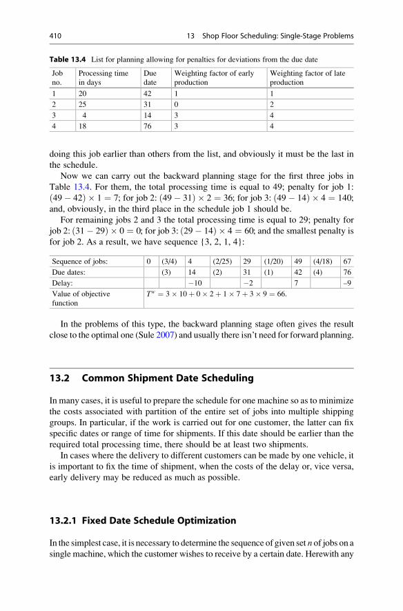
doing this job earlier than others from the list, and obviously it must be the last in
the schedule.
Now we can carry out the backward planning stage for the first three jobs in
Table 13.4. For them, the total processing time is equal to 49; penalty for job 1:
49� 42ð Þ � 1 ¼ 7; for job 2: 49� 31ð Þ � 2 ¼ 36; for job 3: 49� 14ð Þ � 4 ¼ 140;
and, obviously, in the third place in the schedule job 1 should be.
For remaining jobs 2 and 3 the total processing time is equal to 29; penalty for
job 2: 31� 29ð Þ � 0 ¼ 0; for job 3: 29� 14ð Þ � 4 ¼ 60; and the smallest penalty is
for job 2. As a result, we have sequence {3, 2, 1, 4}:
Sequence of jobs: 0 (3/4) 4 (2/25) 29 (1/20) 49 (4/18) 67
Due dates: (3) 14 (2) 31 (1) 42 (4) 76
Delay: �10 �2 7 –9
Value of objective
function
Tw ¼ 3� 10þ 0� 2þ 1� 7þ 3� 9 ¼ 66.
In the problems of this type, the backward planning stage often gives the result
close to the optimal one (Sule 2007) and usually there isn’t need for forward planning.
13.2 Common Shipment Date Scheduling
In many cases, it is useful to prepare the schedule for one machine so as to minimize
the costs associated with partition of the entire set of jobs into multiple shipping
groups. In particular, if the work is carried out for one customer, the latter can fix
specific dates or range of time for shipments. If this date should be earlier than the
required total processing time, there should be at least two shipments.
In cases where the delivery to different customers can be made by one vehicle, it
is important to fix the time of shipment, when the costs of the delay or, vice versa,
early delivery may be reduced as much as possible.
13.2.1 Fixed Date Schedule Optimization
In the simplest case, it is necessary to determine the sequence of given set n of jobs on asingle machine, which the customer wishes to receive by a certain date. Herewith any
Table 13.4 List for planning allowing for penalties for deviations from the due date
Job
no.
Processing time
in days
Due
date
Weighting factor of early
production
Weighting factor of late
production
1 20 42 1 1
2 25 31 0 2
3 4 14 3 4
4 18 76 3 4
410 13 Shop Floor Scheduling: Single-Stage Problems
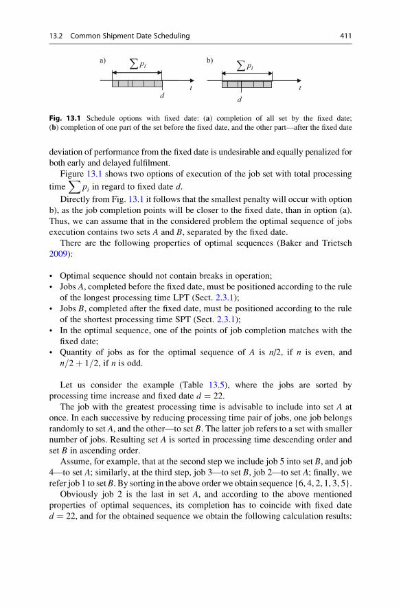
deviation of performance from the fixed date is undesirable and equally penalized for
both early and delayed fulfilment.
Figure 13.1 shows two options of execution of the job set with total processing
timeX
pi in regard to fixed date d.
Directly from Fig. 13.1 it follows that the smallest penalty will occur with option
b), as the job completion points will be closer to the fixed date, than in option (a).
Thus, we can assume that in the considered problem the optimal sequence of jobs
execution contains two sets A and B, separated by the fixed date.
There are the following properties of optimal sequences (Baker and Trietsch
2009):
• Optimal sequence should not contain breaks in operation;
• Jobs A, completed before the fixed date, must be positioned according to the rule
of the longest processing time LPT (Sect. 2.3.1);
• Jobs B, completed after the fixed date, must be positioned according to the rule
of the shortest processing time SPT (Sect. 2.3.1);
• In the optimal sequence, one of the points of job completion matches with the
fixed date;
• Quantity of jobs as for the optimal sequence of A is n/2, if n is even, and
n=2þ 1=2, if n is odd.
Let us consider the example (Table 13.5), where the jobs are sorted by
processing time increase and fixed date d ¼ 22.
The job with the greatest processing time is advisable to include into set A at
once. In each successive by reducing processing time pair of jobs, one job belongs
randomly to set A, and the other—to set B. The latter job refers to a set with smaller
number of jobs. Resulting set A is sorted in processing time descending order and
set B in ascending order.
Assume, for example, that at the second step we include job 5 into set B, and job4—to set A; similarly, at the third step, job 3—to set B, job 2—to set A; finally, werefer job 1 to set B. By sorting in the above order we obtain sequence {6, 4, 2, 1, 3, 5}.
Obviously job 2 is the last in set A, and according to the above mentioned
properties of optimal sequences, its completion has to coincide with fixed date
d ¼ 22, and for the obtained sequence we obtain the following calculation results:
td d
t
a) b)ip ip
Fig. 13.1 Schedule options with fixed date: (a) completion of all set by the fixed date;
(b) completion of one part of the set before the fixed date, and the other part—after the fixed date
13.2 Common Shipment Date Scheduling 411
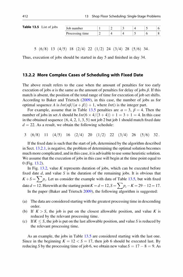
5 ð6=8Þ 13 ð4=5Þ 18 ð2=4Þ 22 ð1=2Þ 24 ð3=4Þ 28 ð5=6Þ 34 :
Thus, execution of jobs should be started in day 5 and finished in day 34.
13.2.2 More Complex Cases of Scheduling with Fixed Date
The above result refers to the case when the amount of penalties for too early
execution of jobs α is the same as the amount of penalties for delay of jobs β. If thismatch is absent, the position of the total range of time for execution of job set shifts.
According to Baker and Trietsch (2009), in this case, the number of jobs as for
optimal sequence A is Int nβ= αþ βð Þð Þ þ 1, where Int() is the integer part.For example, assume that in Table 13.5 penalties are α ¼ 3, β ¼ 4. Then the
number of jobs in set A should be Int 6� 4= 3þ 4ð Þð Þ þ 1 ¼ 3þ 1 ¼ 4. In this case
in the obtained sequence {6, 4, 2, 1, 3, 5} not job 2 but job 1 should match fixed date
d ¼ 22. As a result, we obtain the following schedule:
3 6=8ð Þ 11 4=5ð Þ 16 2=4ð Þ 20 1=2ð Þ 22 3=4ð Þ 26 5=6ð Þ 32 :
If the fixed date is such that the start of job, determined by the algorithm described
in Sect. 13.2.1, is negative, the problem of determining the optimal solution becomes
muchmore complicated, and in this case, it is advisable to use some heuristic solution.
We assume that the execution of jobs in this case will begin at the time point equal to
0 (Fig. 13.2).
In Fig. 13.2, value K represents duration of jobs, which can be executed before
fixed date d, and value S is the duration of the remaining jobs. It is obvious that
KþS¼X
pi. Let us consider the example with data of Table 13.5, but with fixed
dated¼ 12. Herewith at the starting pointK¼ d¼ 12,S¼X
pi�K¼ 29�12¼ 17.
In the paper (Baker and Trietsch 2009), the following algorithm is suggested:
(a) The data are considered starting with the greatest processing time in descending
order.
(b) If K > S, the job is put on the closest allowable position, and value K is
reduced by the relevant processing time.
(c) IfK � S, the job is put on the last allowable position, and value S is reduced bythe relevant processing time.
As an example, the jobs in Table 13.5 are considered starting with the last one.
Since in the beginning K ¼ 12 < S ¼ 17, then job 6 should be executed last. By
reducing S by the processing time of job 6, we obtain new valueS ¼ 17� 8 ¼ 9. As
Table 13.5 List of jobs Job number 1 2 3 4 5 6
Processing time 2 4 4 5 6 8
412 13 Shop Floor Scheduling: Single-Stage Problems
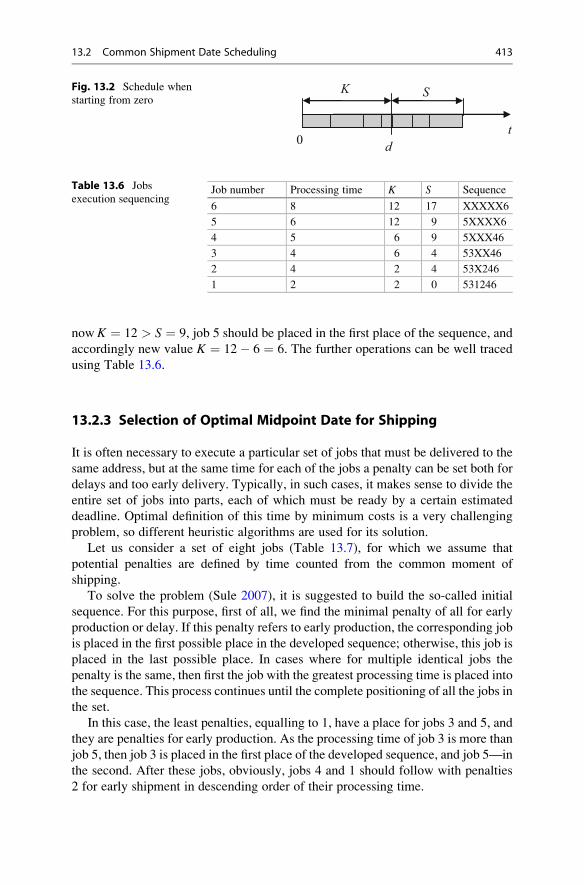
now K ¼ 12 > S ¼ 9, job 5 should be placed in the first place of the sequence, and
accordingly new value K ¼ 12� 6 ¼ 6. The further operations can be well traced
using Table 13.6.
13.2.3 Selection of Optimal Midpoint Date for Shipping
It is often necessary to execute a particular set of jobs that must be delivered to the
same address, but at the same time for each of the jobs a penalty can be set both for
delays and too early delivery. Typically, in such cases, it makes sense to divide the
entire set of jobs into parts, each of which must be ready by a certain estimated
deadline. Optimal definition of this time by minimum costs is a very challenging
problem, so different heuristic algorithms are used for its solution.
Let us consider a set of eight jobs (Table 13.7), for which we assume that
potential penalties are defined by time counted from the common moment of
shipping.
To solve the problem (Sule 2007), it is suggested to build the so-called initial
sequence. For this purpose, first of all, we find the minimal penalty of all for early
production or delay. If this penalty refers to early production, the corresponding job
is placed in the first possible place in the developed sequence; otherwise, this job is
placed in the last possible place. In cases where for multiple identical jobs the
penalty is the same, then first the job with the greatest processing time is placed into
the sequence. This process continues until the complete positioning of all the jobs in
the set.
In this case, the least penalties, equalling to 1, have a place for jobs 3 and 5, and
they are penalties for early production. As the processing time of job 3 is more than
job 5, then job 3 is placed in the first place of the developed sequence, and job 5—in
the second. After these jobs, obviously, jobs 4 and 1 should follow with penalties
2 for early shipment in descending order of their processing time.
dt
K S
0
Fig. 13.2 Schedule when
starting from zero
Table 13.6 Jobs
execution sequencingJob number Processing time K S Sequence
6 8 12 17 XXXXX6
5 6 12 9 5XXXX6
4 5 6 9 5XXX46
3 4 6 4 53XX46
2 4 2 4 53X246
1 2 2 0 531246
13.2 Common Shipment Date Scheduling 413
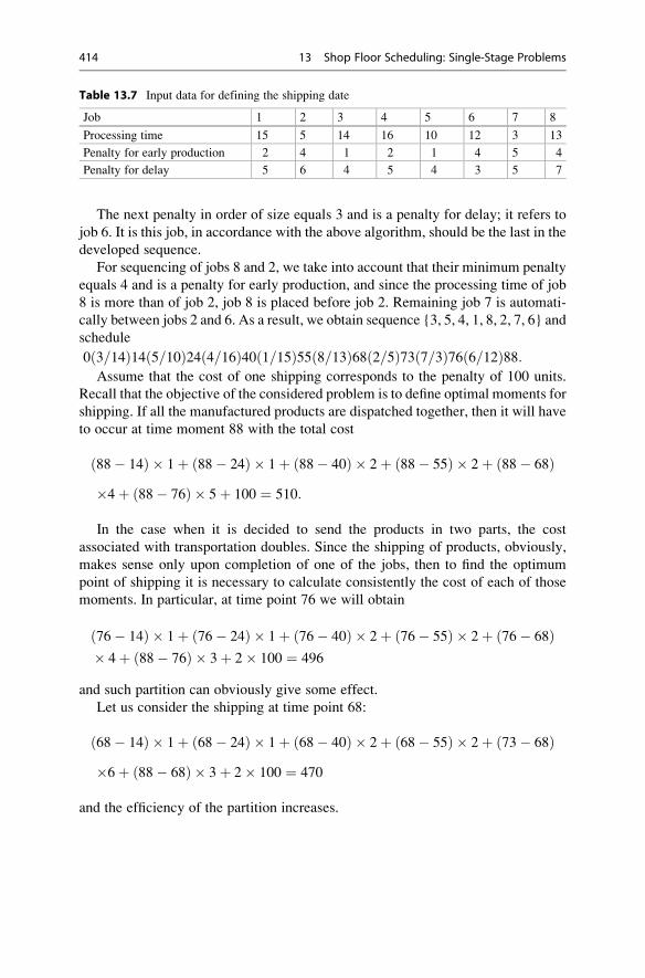
The next penalty in order of size equals 3 and is a penalty for delay; it refers to
job 6. It is this job, in accordance with the above algorithm, should be the last in the
developed sequence.
For sequencing of jobs 8 and 2, we take into account that their minimum penalty
equals 4 and is a penalty for early production, and since the processing time of job
8 is more than of job 2, job 8 is placed before job 2. Remaining job 7 is automati-
cally between jobs 2 and 6. As a result, we obtain sequence {3, 5, 4, 1, 8, 2, 7, 6} and
schedule
0 3=14ð Þ14 5=10ð Þ24 4=16ð Þ40 1=15ð Þ55 8=13ð Þ68 2=5ð Þ73 7=3ð Þ76 6=12ð Þ88:Assume that the cost of one shipping corresponds to the penalty of 100 units.
Recall that the objective of the considered problem is to define optimal moments for
shipping. If all the manufactured products are dispatched together, then it will have
to occur at time moment 88 with the total cost
88� 14ð Þ � 1þ 88� 24ð Þ � 1þ 88� 40ð Þ � 2þ 88� 55ð Þ � 2þ 88� 68ð Þ�4þ 88� 76ð Þ � 5þ 100 ¼ 510:
In the case when it is decided to send the products in two parts, the cost
associated with transportation doubles. Since the shipping of products, obviously,
makes sense only upon completion of one of the jobs, then to find the optimum
point of shipping it is necessary to calculate consistently the cost of each of those
moments. In particular, at time point 76 we will obtain
76� 14ð Þ � 1þ 76� 24ð Þ � 1þ 76� 40ð Þ � 2þ 76� 55ð Þ � 2þ 76� 68ð Þ� 4þ 88� 76ð Þ � 3þ 2� 100 ¼ 496
and such partition can obviously give some effect.
Let us consider the shipping at time point 68:
68� 14ð Þ � 1þ 68� 24ð Þ � 1þ 68� 40ð Þ � 2þ 68� 55ð Þ � 2þ 73� 68ð Þ�6þ 88� 68ð Þ � 3þ 2� 100 ¼ 470
and the efficiency of the partition increases.
Table 13.7 Input data for defining the shipping date
Job 1 2 3 4 5 6 7 8
Processing time 15 5 14 16 10 12 3 13
Penalty for early production 2 4 1 2 1 4 5 4
Penalty for delay 5 6 4 5 4 3 5 7
414 13 Shop Floor Scheduling: Single-Stage Problems
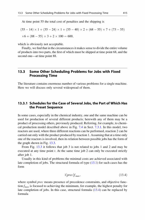
At time point 55 the total cost of penalties and the shipping is
55� 14ð Þ � 1þ 55� 24ð Þ � 1þ 55� 40ð Þ � 2þ 68� 55ð Þ � 7þ 73� 55ð Þ�6þ 88� 55ð Þ � 3þ 2� 100 ¼ 600;
which is obviously not acceptable.
Finally, we find that in the circumstances it makes sense to divide the entire volume
of products into two parts, the first of which must be shipped at time point 68, and the
second one—at time point 88.
13.3 Some Other Scheduling Problems for Jobs with FixedProcessing Time
The literature contains enormous number of various problems for a single machine.
Here we will discuss only several widespread of them.
13.3.1 Schedules for the Case of Several Jobs, the Part of Which Hasthe Preset Sequence
In some cases, especially in the chemical industry, one and the same machine can be
used for production of several different products; herewith any of them may be a
product of processing others, previously produced. Referring, for example, to chemi-
cal production model described above in Fig. 7.4 in Sect. 7.3.1. In this model, two
reactors are used, where three different reactions can be performed, reaction 2 can be
carried out only with the product produced by reaction 1. Assuming that at a time only
one of the reactors is involved, then its relation between possible jobs has the form of
the graph shown in Fig. 13.3.
From Fig. 13.3 it follows that job 3 is not related to jobs 1 and 2 and may be
executed at any time point t. At the same time job 2 can only be executed strictly
after job 1.
Usually in this kind of problems the minimal costs are achieved associated with
late completion of jobs. The structural formula of type (13.1) for such cases has the
form
1��prec��fmax; ð13:4Þ
where symbol prec means presence of precedence constraints, and objective func-
tion fmax is focused to achieving the minimum, for example, the highest penalty for
late completion of jobs. In this case, structural formula (13.4) can be replaced by
formula
13.3 Some Other Scheduling Problems for Jobs with Fixed Processing Time 415
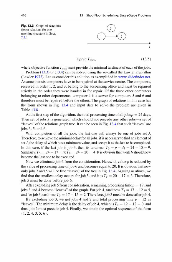
1��prec��Tmax; ð13:5Þ
where objective function Tmax must provide the minimal tardiness of each of the jobs.
Problem (13.3) or (13.4) can be solved using the so-called the Lawler algorithm
(Lawler 1973). Let us consider this solution as exemplified in www.slidefinder.net.
Assume that six computers have to be repaired at the service centre. The computers,
received in order 1, 2, and 3, belong to the accounting office and must be repaired
strictly in the order they were handed in for repair. Of the three other computers
belonging to other departments, computer 4 is a server for computers 5 and 6 and
therefore must be repaired before the others. The graph of relations in this case has
the form shown in Fig. 13.4 and input data to solve the problem are given in
Table 13.8.
At the first step of the algorithm, the total processing time of all jobsp ¼ 24days.
Then set of jobs J is generated, which should not precede any other jobs—a set of
“leaves” of the relations graph tree. It can be seen in Fig. 13.4 that such “leaves” are
jobs 3, 5, and 6.
With completion of all the jobs, the last one will always be one of jobs set J.Therefore, to achieve theminimal delay for all jobs, it is necessary to find an element of
set J, the delay of which has aminimum value, and accept it as the last to be completed.
In this case, if the last job is job 3, then its tardiness T3 ¼ p� d3 ¼ 24� 15 ¼ 9.
Similarly,T5 ¼ 24� 17 ¼ 7;T6 ¼ 24� 20 ¼ 4. It is obvious that work 6 should now
become the last one to be executed.
Now we eliminate job 6 from the consideration. Herewith value p is reduced by
the value of processing time of job 6 and becomes equal to 20. It is obvious that now
only jobs 3 and 5 will be free “leaves” of the tree in Fig. 13.4. Arguing as above, we
find that the smallest delay occurs for job 5, and it is T5 ¼ 20� 17 ¼ 3. Therefore,
job 5 must be done before job 6.
After excluding job 5 from consideration, remaining processing timep ¼ 17, and
jobs 3 and 4 become “leaves” of the graph. For job 4, tardiness T4 ¼ 17� 12 ¼ 5,
and for job 3, tardinessT3 ¼ 17� 15 ¼ 2. Therefore, job 3 must be done after job 4.
By excluding job 3, we get jobs 4 and 2 and total processing time p ¼ 12 as
“leaves”. The minimum delay is the delay of job 4, which isT4 ¼ 12� 12 ¼ 0, and
thus, job 2 must precede job 4. Finally, we obtain the optimal sequence of the form
{1, 2, 4, 3, 5, 6}.
1 2
3
t
Fig. 13.3 Graph of reactions
(jobs) relations for one
machine (reactor) in Sect.
7.3.1
416 13 Shop Floor Scheduling: Single-Stage Problems

13.3.2 Scheduling of Jobs with Different Arrival Time
If the jobs to be executed on the machine are available at different times, i.e. upon
receipt of materials or work pieces, then the optimization problem by any criteria
becomes difficult. In these cases, mainly heuristic methods are used to optimally
load the machine with those jobs that are possible at the time of the machine release
from the previous job or a group of such jobs. Let us consider the example, the data
for which are shown in Table 13.9.
Suppose that at the initial moment of planning the machine is free. In this case,
job 1 can be started first, which arrives at time point 2. In the absence of external
causes, this job can be completed at time point C1 ¼ r1 þ p1 ¼ 2þ 5 ¼ 7. Since
this execution date is less than the required execution date d1 ¼ 9, the penalty for
delay of job 1 is absent. Thus, the initial part of the planning sequence has the form
2 1=5ð Þ 7 :
At this point, all necessary materials for the job 2 have to be near the machine,
and other works are still non-available. Obviously, the start point of job 2 in this
case is defined asmax C1; r2ð Þ ¼ max 7; 5ð Þ ¼ 7. Job 2 can be completed at time point
C2¼C1þp2¼7þ7¼14with a penalty for delay C2�d2ð Þ�c2¼ 14�12ð Þ�1¼2.
The sequence of planning takes the form
2 1=5ð Þ 7 2=7ð Þ 14 :
By time point 14 it appears to be possible to execute three jobs 4, 5, and 6 at once on
themachine. Since there are penalties for delay, then themost reasonableway to select
the sequence of these jobs is to use the algorithm outlined above in Sect. 13.1.2.
When performing backward planning stage of this algorithm first we define the
total processing time p for all possible jobs. In this case, these are jobs 4, 5, and
1 2 3
t
4
5
6
Fig. 13.4 The graph of
relations in case of computer
repairing
Table 13.8 List of orders
for repairComputer no. 1 2 3 4 5 6
Processing time 3 2 5 7 3 4
Due date 4 9 15 12 17 20
13.3 Some Other Scheduling Problems for Jobs with Fixed Processing Time 417
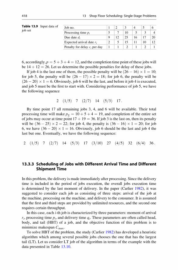
6, accordingly,p ¼ 5þ 3þ 4 ¼ 12, and the completion time point of these jobs will
be 14þ 12 ¼ 26. Let us determine the possible penalties for delay of these jobs.
If job 4 is the last one of them, the possible penalty will be 26� 16ð Þ � 1 ¼ 10;
for job 5, the penalty will be 26� 17ð Þ � 2 ¼ 18; for job 6, the penalty will be
26� 20ð Þ � 1 ¼ 6. Obviously, job 6 will be the last, and before it job 4 is executed,
and job 5 must be the first to start with. Considering performance of job 5, we have
the following sequence
2 1=5ð Þ 7 2=7ð Þ 14 5=3ð Þ 17 :
By time point 17 all remaining jobs 3, 4, and 6 will be available. Their total
processing time will make pΣ ¼ 10þ 5þ 4 ¼ 19, and completion of the entire set
of jobs may occur at time point 17þ 19 ¼ 36. If job 3 is the last on, then its penalty
will be 36� 25ð Þ � 2 ¼ 22; for job 4, the penalty is 36� 16ð Þ � 1 ¼ 20; for job
6, we have 36� 20ð Þ � 1 ¼ 16. Obviously, job 6 should be the last and job 4 the
last but one. Eventually, we have the following sequence:
2 1=5ð Þ 7 2=7ð Þ 14 5=3ð Þ 17 3=10ð Þ 27 4=5ð Þ 32 6=4ð Þ 36 :
13.3.3 Scheduling of Jobs with Different Arrival Time and DifferentShipment Time
In this problem, the delivery is made immediately after processing. Since the delivery
time is included in the period of jobs execution, the overall jobs execution time
is determined by the last moment of delivery. In the paper (Carlier 1982), it was
suggested to consider each job as consisting of three steps: arrival of the job at
the machine, processing on the machine, and delivery to the consumer. It is assumed
that the first and third steps are provided by unlimited resources, and the second one
requires certain throughput.
In this case, each i-th job is characterized by three parameters: moment of arrival
ri, processing time pi, and delivery time qi. These parameters are often called head,
body, and tail (HBT) of a job, and the objective function of this problem is to
minimize makespan Cmax.
To solve HBT of the problem, the study (Carlier 1982) has developed a heuristic
algorithm which among several possible jobs chooses the one that has the largest
tail (LT). Let us consider LT job of the algorithm in terms of the example with the
data presented in Table 13.10.
Table 13.9 Input data of
job setJob no. 1 2 3 4 5 6
Processing time pi 5 7 10 5 3 4
Due date di 9 12 25 16 17 20
Expected arrival date ri 2 5 15 11 10 12
Penalty for delay ci per day 1 1 2 1 2 1
418 13 Shop Floor Scheduling: Single-Stage Problems
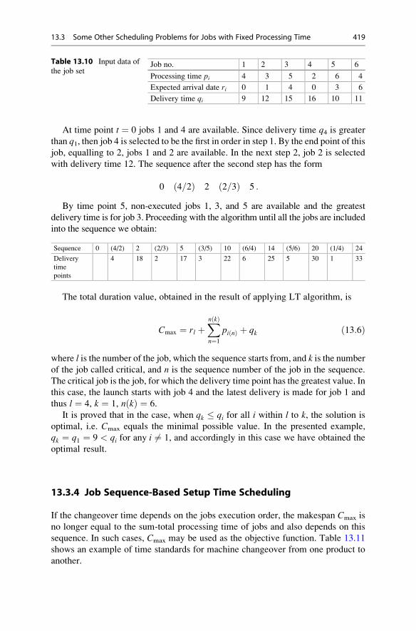
At time point t ¼ 0 jobs 1 and 4 are available. Since delivery time q4 is greaterthan q1, then job 4 is selected to be the first in order in step 1. By the end point of thisjob, equalling to 2, jobs 1 and 2 are available. In the next step 2, job 2 is selected
with delivery time 12. The sequence after the second step has the form
0 4=2ð Þ 2 2=3ð Þ 5 :
By time point 5, non-executed jobs 1, 3, and 5 are available and the greatest
delivery time is for job 3. Proceeding with the algorithm until all the jobs are included
into the sequence we obtain:
Sequence 0 (4/2) 2 (2/3) 5 (3/5) 10 (6/4) 14 (5/6) 20 (1/4) 24
Delivery
time
points
4 18 2 17 3 22 6 25 5 30 1 33
The total duration value, obtained in the result of applying LT algorithm, is
Cmax ¼ rl þXn kð Þ
n¼1
pi nð Þ þ qk ð13:6Þ
where l is the number of the job, which the sequence starts from, and k is the number
of the job called critical, and n is the sequence number of the job in the sequence.
The critical job is the job, for which the delivery time point has the greatest value. In
this case, the launch starts with job 4 and the latest delivery is made for job 1 and
thus l ¼ 4, k ¼ 1, n kð Þ ¼ 6.
It is proved that in the case, when qk � qi for all i within l to k, the solution is
optimal, i.e. Cmax equals the minimal possible value. In the presented example,
qk ¼ q1 ¼ 9 < qi for any i 6¼ 1, and accordingly in this case we have obtained the
optimal result.
13.3.4 Job Sequence-Based Setup Time Scheduling
If the changeover time depends on the jobs execution order, the makespan Cmax is
no longer equal to the sum-total processing time of jobs and also depends on this
sequence. In such cases, Cmax may be used as the objective function. Table 13.11
shows an example of time standards for machine changeover from one product to
another.
Table 13.10 Input data of
the job setJob no. 1 2 3 4 5 6
Processing time pi 4 3 5 2 6 4
Expected arrival date ri 0 1 4 0 3 6
Delivery time qi 9 12 15 16 10 11
13.3 Some Other Scheduling Problems for Jobs with Fixed Processing Time 419
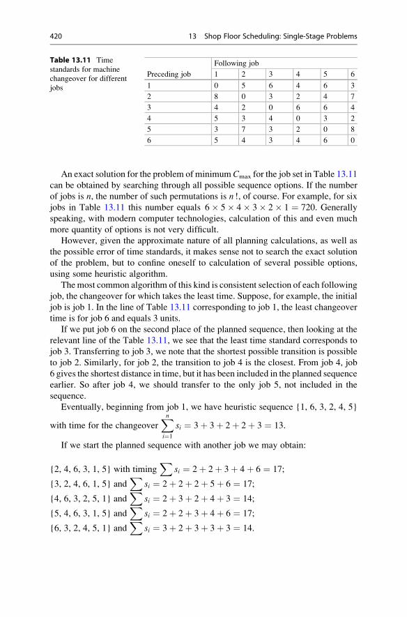
An exact solution for the problem of minimum Cmax for the job set in Table 13.11
can be obtained by searching through all possible sequence options. If the number
of jobs is n, the number of such permutations is n !, of course. For example, for six
jobs in Table 13.11 this number equals 6� 5� 4� 3� 2� 1 ¼ 720. Generally
speaking, with modern computer technologies, calculation of this and even much
more quantity of options is not very difficult.
However, given the approximate nature of all planning calculations, as well as
the possible error of time standards, it makes sense not to search the exact solution
of the problem, but to confine oneself to calculation of several possible options,
using some heuristic algorithm.
Themost common algorithm of this kind is consistent selection of each following
job, the changeover for which takes the least time. Suppose, for example, the initial
job is job 1. In the line of Table 13.11 corresponding to job 1, the least changeover
time is for job 6 and equals 3 units.
If we put job 6 on the second place of the planned sequence, then looking at the
relevant line of the Table 13.11, we see that the least time standard corresponds to
job 3. Transferring to job 3, we note that the shortest possible transition is possible
to job 2. Similarly, for job 2, the transition to job 4 is the closest. From job 4, job
6 gives the shortest distance in time, but it has been included in the planned sequence
earlier. So after job 4, we should transfer to the only job 5, not included in the
sequence.
Eventually, beginning from job 1, we have heuristic sequence {1, 6, 3, 2, 4, 5}
with time for the changeoverXni¼1
si ¼ 3þ 3þ 2þ 2þ 3 ¼ 13.
If we start the planned sequence with another job we may obtain:
{2, 4, 6, 3, 1, 5} with timingX
si ¼ 2þ 2þ 3þ 4þ 6 ¼ 17;
{3, 2, 4, 6, 1, 5} andX
si ¼ 2þ 2þ 2þ 5þ 6 ¼ 17;
{4, 6, 3, 2, 5, 1} andX
si ¼ 2þ 3þ 2þ 4þ 3 ¼ 14;
{5, 4, 6, 3, 1, 5} andX
si ¼ 2þ 2þ 3þ 4þ 6 ¼ 17;
{6, 3, 2, 4, 5, 1} andX
si ¼ 3þ 2þ 3þ 3þ 3 ¼ 14.
Table 13.11 Time
standards for machine
changeover for different
jobs
Preceding job
Following job
1 2 3 4 5 6
1 0 5 6 4 6 3
2 8 0 3 2 4 7
3 4 2 0 6 6 4
4 5 3 4 0 3 2
5 3 7 3 2 0 8
6 5 4 3 4 6 0
420 13 Shop Floor Scheduling: Single-Stage Problems
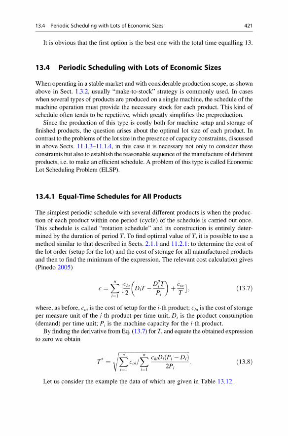
It is obvious that the first option is the best one with the total time equalling 13.
13.4 Periodic Scheduling with Lots of Economic Sizes
When operating in a stable market and with considerable production scope, as shown
above in Sect. 1.3.2, usually “make-to-stock” strategy is commonly used. In cases
when several types of products are produced on a single machine, the schedule of the
machine operation must provide the necessary stock for each product. This kind of
schedule often tends to be repetitive, which greatly simplifies the preproduction.
Since the production of this type is costly both for machine setup and storage of
finished products, the question arises about the optimal lot size of each product. In
contrast to the problems of the lot size in the presence of capacity constraints, discussed
in above Sects. 11.1.3–11.1.4, in this case it is necessary not only to consider these
constraints but also to establish the reasonable sequence of themanufacture of different
products, i.e. to make an efficient schedule. A problem of this type is called Economic
Lot Scheduling Problem (ELSP).
13.4.1 Equal-Time Schedules for All Products
The simplest periodic schedule with several different products is when the produc-
tion of each product within one period (cycle) of the schedule is carried out once.
This schedule is called “rotation schedule” and its construction is entirely deter-
mined by the duration of period T. To find optimal value of T, it is possible to use amethod similar to that described in Sects. 2.1.1 and 11.2.1: to determine the cost of
the lot order (setup for the lot) and the cost of storage for all manufactured products
and then to find the minimum of the expression. The relevant cost calculation gives
(Pinedo 2005)
c ¼Xni¼1
�chi2
DiT � D2i T
Pi
� �þ coi
T
; ð13:7Þ
where, as before, coi is the cost of setup for the i-th product; chi is the cost of storageper measure unit of the i-th product per time unit, Di is the product consumption
(demand) per time unit; Pi is the machine capacity for the i-th product.
By finding the derivative from Eq. (13.7) for T, and equate the obtained expressionto zero we obtain
T* ¼ffiffiffiffiffiffiffiffiffiffiffiffiffiffiffiffiffiffiffiffiffiffiffiffiffiffiffiffiffiffiffiffiffiffiffiffiffiffiffiffiffiffiffiffiffiffiffiffiffiffiffiffiXni¼1
coi=Xni¼1
chiDi Pi � Dið Þ2Pi
s: ð13:8Þ
Let us consider the example the data of which are given in Table 13.12.
13.4 Periodic Scheduling with Lots of Economic Sizes 421
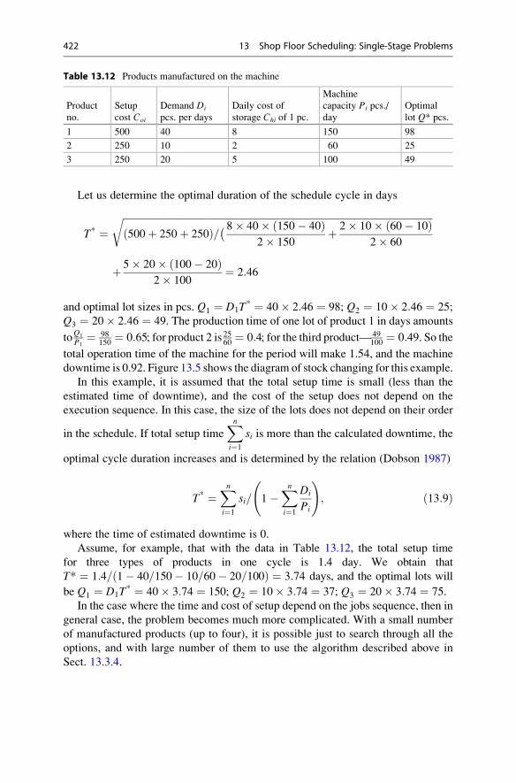
Let us determine the optimal duration of the schedule cycle in days
T* ¼ffiffiffiffiffiffiffiffiffiffiffiffiffiffiffiffiffiffiffiffiffiffiffiffiffiffiffiffiffiffiffiffiffiffiffiffiffiffiffiffiffiffiffiffiffiffiffiffiffiffiffiffiffiffiffiffiffiffiffiffiffiffiffiffiffiffiffiffiffiffiffiffiffiffiffiffiffiffiffiffiffiffiffiffiffiffiffiffiffiffiffiffiffiffiffiffiffiffiffiffiffiffiffiffiffiffiffiffiffiffiffiffiffiffiffiffiffiffiffiffiffiffiffiffiffiffiffi500þ 250þ 250ð Þ=� 8� 40� 150� 40ð Þ
2� 150þ 2� 10� 60� 10ð Þ
2� 60
r
þ 5� 20� 100� 20ð Þ2� 100
¼ 2:46
and optimal lot sizes in pcs. Q1 ¼ D1T* ¼ 40� 2:46 ¼ 98; Q2 ¼ 10� 2:46 ¼ 25;
Q3 ¼ 20� 2:46 ¼ 49. The production time of one lot of product 1 in days amounts
toQ1
P1¼ 98
150¼ 0:65; for product 2 is 25
60¼ 0:4; for the third product—49
100¼ 0:49. So the
total operation time of the machine for the period will make 1.54, and the machine
downtime is 0.92. Figure 13.5 shows the diagram of stock changing for this example.
In this example, it is assumed that the total setup time is small (less than the
estimated time of downtime), and the cost of the setup does not depend on the
execution sequence. In this case, the size of the lots does not depend on their order
in the schedule. If total setup timeXni¼1
si is more than the calculated downtime, the
optimal cycle duration increases and is determined by the relation (Dobson 1987)
T* ¼Xni¼1
si= 1�Xni¼1
Di
Pi
!; ð13:9Þ
where the time of estimated downtime is 0.
Assume, for example, that with the data in Table 13.12, the total setup time
for three types of products in one cycle is 1.4 day. We obtain that
T* ¼ 1:4= 1� 40=150� 10=60� 20=100ð Þ ¼ 3:74 days, and the optimal lots will
be Q1 ¼ D1T* ¼ 40� 3:74 ¼ 150; Q2 ¼ 10� 3:74 ¼ 37; Q3 ¼ 20� 3:74 ¼ 75.
In the case where the time and cost of setup depend on the jobs sequence, then in
general case, the problem becomes much more complicated. With a small number
of manufactured products (up to four), it is possible just to search through all the
options, and with large number of them to use the algorithm described above in
Sect. 13.3.4.
Table 13.12 Products manufactured on the machine
Product
no.
Setup
cost Coi
Demand Di
pcs. per days
Daily cost of
storage Chi of 1 pc.
Machine
capacity Pi pcs./
day
Optimal
lot Q* pcs.
1 500 40 8 150 98
2 250 10 2 60 25
3 250 20 5 100 49
422 13 Shop Floor Scheduling: Single-Stage Problems

13.4.2 Variable-Time Schedules for Different Products
In general, in one schedule cycle, one and the same product can be produced in
several lots. An exact solution of this problem is very difficult to obtain, if possible
at all. However, nowadays there is an effective heuristic method developed in the
paper (Dobson 1987), which is called Frequency Fixing and Sequencing (FFS). The
method consists of three successive stages:
• Theoretical calculation of the relative frequencies of manufacture of each
product;
• Establishing efficient frequencies;
• Determining efficient sequence of lots production.
Obviously, that in one schedule cycle with duration T, the lots of each i-th productcan be produced a number of times, i.e. frequency ωi is an integer. In FFS method,
for reasons of minimum costs, the optimal (not necessarily integer) frequencies of
manufacture of each product are determined, the values of which are rounded then to
integer values. Thus, the problem of the first stage is reduced (Pinedo 2005) to
finding the minimum cost
c ¼Xni¼1
aiT
ωiþXni¼1
coiωi
T; ð13:10Þ
with setup time si constraint
Xni¼1
siωi
T� 1�
Xni¼1
Di
Pi: ð13:11Þ
In expression (13.10)
Product 1
Product 2 Product 3
0
10
20
30
40
50
60
70
80
0 1 2 3 4S
tock
Time
Cycle
Idle timeFig. 13.5 Diagram of stocks
of the manufactured products
with equal cycles
13.4 Periodic Scheduling with Lots of Economic Sizes 423
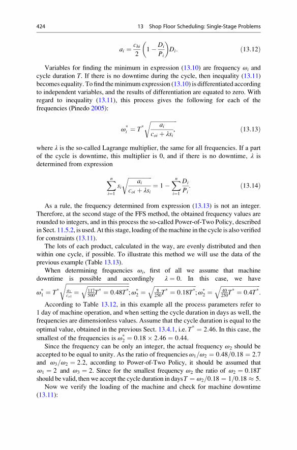
ai ¼ chi2
1� Di
Pi
� �Di: ð13:12Þ
Variables for finding the minimum in expression (13.10) are frequency ωi and
cycle duration T. If there is no downtime during the cycle, then inequality (13.11)
becomes equality. To find theminimum expression (13.10) is differentiated according
to independent variables, and the results of differentiation are equated to zero. With
regard to inequality (13.11), this process gives the following for each of the
frequencies (Pinedo 2005):
ω*i ¼ T*
ffiffiffiffiffiffiffiffiffiffiffiffiffiffiffiffiffiffiffiai
coi þ λsi,
rð13:13Þ
where λ is the so-called Lagrange multiplier, the same for all frequencies. If a part
of the cycle is downtime, this multiplier is 0, and if there is no downtime, λ is
determined from expression
Xni¼1
si
ffiffiffiffiffiffiffiffiffiffiffiffiffiffiffiffiffiai
coi þ λsi
r¼ 1�
Xni¼1
Di
Pi: ð13:14Þ
As a rule, the frequency determined from expression (13.13) is not an integer.
Therefore, at the second stage of the FFS method, the obtained frequency values are
rounded to integers, and in this process the so-called Power-of-Two Policy, described
in Sect. 11.5.2, is used. At this stage, loading of themachine in the cycle is also verified
for constraints (13.11).
The lots of each product, calculated in the way, are evenly distributed and then
within one cycle, if possible. To illustrate this method we will use the data of the
previous example (Table 13.13).
When determining frequencies ωi, first of all we assume that machine
downtime is possible and accordingly λ ¼ 0. In this case, we have
ω*1 ¼ T*
ffiffiffiffiffiffiffiffiffiffiffiffiffiffiffiffiffiffiffiffiffiffiffiffiffiffiffiffiffiffiffiffiffiffiffiffiffiffiffiffiffiffiffiffiffia1co1
¼ffiffiffiffiffiffiffiffiffiffiffiffiffiffiffiffiffiffiffiffiffiffiffiffiffiffiffiffiffiffi117500
T* ¼ 0:48T*qr
;ω*2 ¼
ffiffiffiffiffiffiffiffiffiffiffiffiffiffiffiffiffiffiffiffiffiffiffiffiffiffiffiffiffiffi8250
T* ¼ 0:18T*q
;ω*2 ¼
ffiffiffiffiffiffiffiffiffiffiffiffiffiffiffiffiffiffiffiffiffiffiffiffiffiffiffiffi40250
T* ¼ 0:4T*q
.
According to Table 13.12, in this example all the process parameters refer to
1 day of machine operation, and when setting the cycle duration in days as well, the
frequencies are dimensionless values. Assume that the cycle duration is equal to the
optimal value, obtained in the previous Sect. 13.4.1, i.e. T* ¼ 2:46. In this case, the
smallest of the frequencies is ω*2 ¼ 0:18� 2:46 ¼ 0:44.
Since the frequency can be only an integer, the actual frequency ω2 should be
accepted to be equal to unity. As the ratio of frequenciesω1=ω2 ¼ 0:48=0:18 ¼ 2:7and ω3=ω2 ¼ 2:2, according to Power-of-Two Policy, it should be assumed that
ω1 ¼ 2 and ω3 ¼ 2. Since for the smallest frequency ω2 the ratio of ω2 ¼ 0:18Tshould be valid, thenwe accept the cycle duration in daysT ¼ ω2=0:18 ¼ 1=0:18 � 5.
Now we verify the loading of the machine and check for machine downtime
(13.11):
424 13 Shop Floor Scheduling: Single-Stage Problems
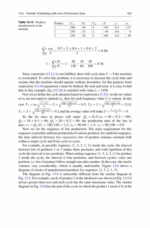
Xni¼1
siωi
T¼ 0:5� 2þ 0:6� 1þ 0:4� 2
5¼ 0:48;
1�Xni¼1
Di
Pi¼ 1� 40
150� 10
60� 20
100¼ 0:36:
Since constraint (13.11) is not fulfilled, then with cycle time T ¼ 5 the machine
is overloaded. To solve this problem, it is necessary to increase the cycle time and
assume that the machine should operate without downtime; for this purpose from
expression (13.14) parameter λ must be defined. By trial and error, it is easy to find
that in this example, Eq. (13.14) is satisfied with value λ ¼ 1450.
Now let us define the cycle duration based on expression (13.13). As the set values
of ωi are not equal to optimal ωi , then for each frequency value Ti is various. In this
case T1 ¼ ω1
ffiffiffiffiffiffiffiffiffiffiffico1þλs1
a1
q¼ 2�
ffiffiffiffiffiffiffiffiffiffiffiffiffiffiffiffiffiffiffiffiffi500þ1450�0:5
117
q¼ 6:5; T2 ¼ 1�
ffiffiffiffiffiffiffiffiffiffiffiffiffiffiffiffiffiffiffiffiffi250þ1450�0:6
8
q¼ 11:8;
T3 ¼ 2�ffiffiffiffiffiffiffiffiffiffiffiffiffiffiffiffiffiffiffiffiffi250þ1450�0:4
40
q¼ 9:2 and the average value will make T ¼ T1þT2þT3
3¼ 9.
So the lot sizes in pieces will make Q1 ¼ D1T=ω1 ¼ 40� 9=2 ¼ 180 ;
Q2 ¼ 10� 9=1 ¼ 90; Q3 ¼ 20� 9=2 ¼ 90; the production time of the lots in
days τ1 ¼ Q1=P1 ¼ 180=150 ¼ 1:2; τ2 ¼ 90=60 ¼ 1:5; τ3 ¼ 90=100 ¼ 0:9.Now we set the sequence of lots production. The main requirement for this
sequence is possibly uniform production of various products. In a uniform sequence,
the time interval between two successive lots of product remains constant both
within a single cycle and from cycle to cycle.
For example, in possible sequence {1, 3, 2, 1, 3} inside the cycle, the interval
between lots of products 1 or 3 makes three positions, and with repetition of this
cycle the interval is two positions. When setting sequence {1, 3, 2, 3, 1} for product
1 inside the cycle, the interval is four positions, and between cycles—only one
position, i.e. lots of product follow straight one after another. In this case, the stocks
volumes vary considerably, which is usually undesirable. Figure 13.6 shows a
diagram of stocks of manufactured products for sequence {1, 3, 2, 1, 3}.
The diagram in Fig. 13.6 is noticeably different from the similar diagram in
Fig. 13.5. For example, stock of product 1 in the idealized case shown in Fig. 13.5 if
always greater than zero and each cycle has the same maximum value. The similar
diagram in Fig. 13.6 has the part of the cycle in which the product 1 stock is 0; at the
Table 13.13 Products
manufactured on the
machine
Product Coi Di Chi Pi si ai
1 500 40 8 150 0.5 117
2 250 10 2 60 0.6 8
3 250 20 5 100 0.4 40
13.4 Periodic Scheduling with Lots of Economic Sizes 425
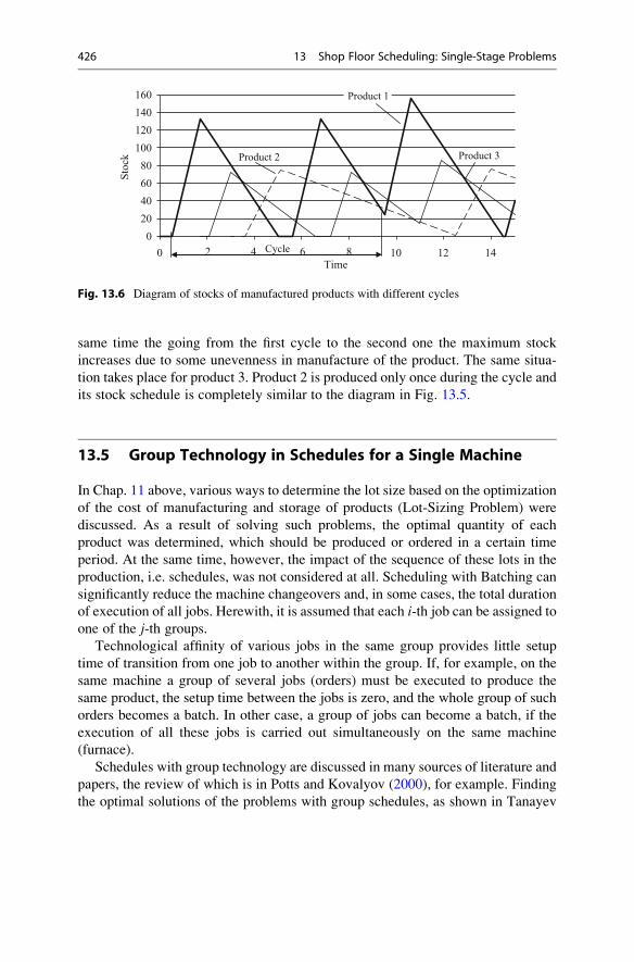
same time the going from the first cycle to the second one the maximum stock
increases due to some unevenness in manufacture of the product. The same situa-
tion takes place for product 3. Product 2 is produced only once during the cycle and
its stock schedule is completely similar to the diagram in Fig. 13.5.
13.5 Group Technology in Schedules for a Single Machine
In Chap. 11 above, various ways to determine the lot size based on the optimization
of the cost of manufacturing and storage of products (Lot-Sizing Problem) were
discussed. As a result of solving such problems, the optimal quantity of each
product was determined, which should be produced or ordered in a certain time
period. At the same time, however, the impact of the sequence of these lots in the
production, i.e. schedules, was not considered at all. Scheduling with Batching can
significantly reduce the machine changeovers and, in some cases, the total duration
of execution of all jobs. Herewith, it is assumed that each i-th job can be assigned toone of the j-th groups.
Technological affinity of various jobs in the same group provides little setup
time of transition from one job to another within the group. If, for example, on the
same machine a group of several jobs (orders) must be executed to produce the
same product, the setup time between the jobs is zero, and the whole group of such
orders becomes a batch. In other case, a group of jobs can become a batch, if the
execution of all these jobs is carried out simultaneously on the same machine
(furnace).
Schedules with group technology are discussed in many sources of literature and
papers, the review of which is in Potts and Kovalyov (2000), for example. Finding
the optimal solutions of the problems with group schedules, as shown in Tanayev
0
20
40
60
80
100
120
140
160
0 2 4 6 8 10 12 14
Sto
ck
Time
Cycle
Product 1
Product 3 Product 2
Fig. 13.6 Diagram of stocks of manufactured products with different cycles
426 13 Shop Floor Scheduling: Single-Stage Problems
et al. (1998), relates to significant computational difficulties, and therefore, as a
rule, each of these studies was performed for each individual case. For practical use,
even if not very accurate, relatively simple solutions suitable for different problems
are required.
13.5.1 Group Scheduling for Series Batches
Let us consider the problem of group scheduling for a single machine with the
minimization of the largest deviation of jobs Lmax in the schedule from the fixed due
dates. We assume that the data in Table 13.14 are planned task for the coming
calendar month, which has 25 working days. The processing time of each out of the
eight jobs is specified in working days, and each of the jobs belongs to one of three
groups. Suppose also that the setup time per group of jobs in working days
s1 ¼ s2 ¼ 1, s3 ¼ 2, and setup time for the job within the group is inconsiderable.
The classification formula of the problem in this case has the form (Appendix C):
1 batch;Cjob
� ��sj��Lmax; ð13:15Þwhere parameter “batch” means that the schedule should be made using the job
grouping; parameter Cjob indicates that after completion of each job the relevant
product leaves the single machine (sequential execution of jobs); parameter sjindicates the necessity to take into account the time for setup with different value
for each group.
Let us position the jobs of each group according to EDD (Earliest Due Date)
rule, described above in Sect. 2.3.1. For group 1 we obtain sequence {1, 7, 3}, for
group 2—sequence {4, 6, 8}, and for group 3—{2, 5}. Suppose the initial time
point of the setup of some j-th group equals tj. When executing the jobs within the
group in the specified sequence the deviation from the required date of execution
will be
Lji ¼ tj þ sj þ pj1 þ pj2 þ . . .þ pji � dji: ð13:16Þ
Let us determine the value of processing time, which remains in the j-th group
after completion of the i-th job.
Table 13.14 Input data of job set
Job no. 1 2 3 4 5 6 7 8
Processing time pi 3 5 6 5 2 4 2 3
Due date di 9 12 25 16 17 20 15 20
Job group 1 3 1 2 3 2 1 2
13.5 Group Technology in Schedules for a Single Machine 427
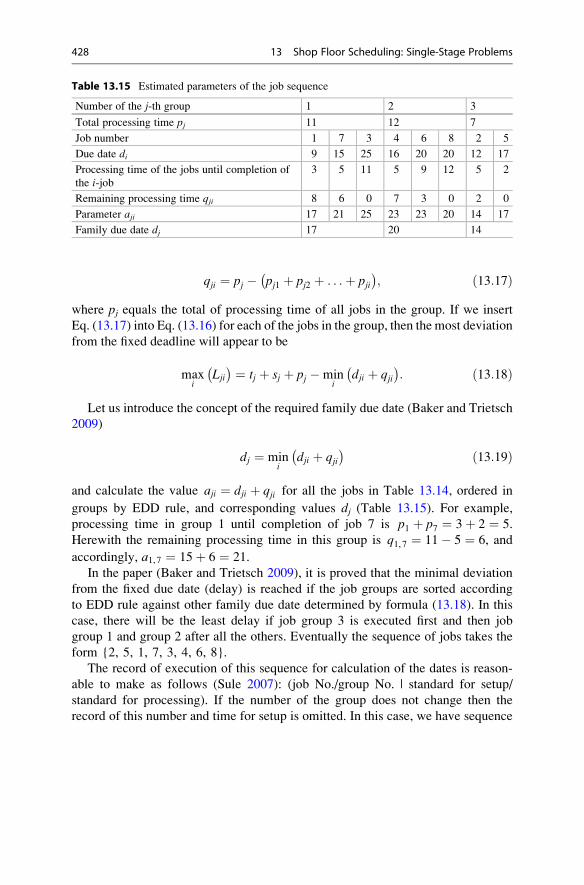
qji ¼ pj � pj1 þ pj2 þ . . .þ pji�
; ð13:17Þ
where pj equals the total of processing time of all jobs in the group. If we insert
Eq. (13.17) into Eq. (13.16) for each of the jobs in the group, then the most deviation
from the fixed deadline will appear to be
maxi
Lji� ¼ tj þ sj þ pj �min
idji þ qji�
: ð13:18Þ
Let us introduce the concept of the required family due date (Baker and Trietsch
2009)
dj ¼ mini
dji þ qji� ð13:19Þ
and calculate the value aji ¼ dji þ qji for all the jobs in Table 13.14, ordered in
groups by EDD rule, and corresponding values dj (Table 13.15). For example,
processing time in group 1 until completion of job 7 is p1 þ p7 ¼ 3þ 2 ¼ 5.
Herewith the remaining processing time in this group is q1,7 ¼ 11� 5 ¼ 6, and
accordingly, a1,7 ¼ 15þ 6 ¼ 21.
In the paper (Baker and Trietsch 2009), it is proved that the minimal deviation
from the fixed due date (delay) is reached if the job groups are sorted according
to EDD rule against other family due date determined by formula (13.18). In this
case, there will be the least delay if job group 3 is executed first and then job
group 1 and group 2 after all the others. Eventually the sequence of jobs takes the
form {2, 5, 1, 7, 3, 4, 6, 8}.
The record of execution of this sequence for calculation of the dates is reason-
able to make as follows (Sule 2007): (job No./group No. | standard for setup/
standard for processing). If the number of the group does not change then the
record of this number and time for setup is omitted. In this case, we have sequence
Table 13.15 Estimated parameters of the job sequence
Number of the j-th group 1 2 3
Total processing time pj 11 12 7
Job number 1 7 3 4 6 8 2 5
Due date di 9 15 25 16 20 20 12 17
Processing time of the jobs until completion of
the i-job3 5 11 5 9 12 5 2
Remaining processing time qji 8 6 0 7 3 0 2 0
Parameter aji 17 21 25 23 23 20 14 17
Family due date dj 17 20 14
428 13 Shop Floor Scheduling: Single-Stage Problems
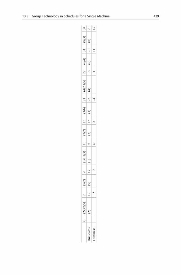
0(2/3|2/5)
7(5/2)
9(1/1|1/3)
13
(7/2)
15
(3/6)
21
(4/2|1/5)
27
(6/4)
31
(8/3)
34
Duedates
(2)
12
(5)
17
(1)
9(7)
15
(3)
25
(4)
16
(6)
20
(8)
20
Tardiness
�5�8
40
–4
11
11
14
13.5 Group Technology in Schedules for a Single Machine 429
It is obvious that the set scope of jobs does not fit in the available time fund, and
for its execution, for example, the quantity of working shifts should be increased. At
that the processing time in working days will decrease accordingly, but the optimal
sequence of their execution will not change.
13.5.2 Group Scheduling for Parallel Batches with MinimumTardiness Criterion
Simultaneous execution of multiple jobs on one machine is typical for treatment in
furnace, bath, and like equipment, which can accommodate several batches of different
products, for which the processing mode is the same. In such cases, the collection of all
such products makes one load batch for which processing is continuous. Herewith, no
other jobs are loaded in the machine until the end of the treatment process.
If each job takes about the same space, the machine capacity can be defined as
allowable quantity b of simultaneously performed jobs of duration p. Let us considerthe problem of the optimal planning for a machine with parallel execution of jobs, for
which the processing mode is the same, and for an objective function of minimal total
tardiness T for a given set of jobs.
The classification formula of this problem has the form
1 batch;Cbatchð Þ��g ¼ 1��T; ð13:20Þ
where parameter ‘batch” indicated that the schedule should be made using the load
batches consisting of multiple jobs; parameter Cbatch shows parallel execution of all
loaded jobs; parameter g indicated the quantity of job groups requiring different
process settings.
We arrange the jobs in order of expected arrival and consider the example, the
data for which are shown in Table 13.16. The time points of arrival and execution
can be set in hours, shifts, days, etc. Let time p of the treatment process be 3, and the
largest quantity of simultaneous jobs b (machine capacity) is 4.
To solve the problems of this type it is advisable to use a heuristic algorithm with
partial searching through options (Sule 2007). At the first step of the algorithm the
batch combines the jobs received by the time of load planning in order of increasing
due time point. If such jobs are more than the machine capacity, then the joining is
carried out until the quantity of jobs in the batch is equal to permissible load quantity
b. If the jobs are all used up and all the load batches are of the same size, equalling to
b the scheduling stops.
If after scheduling it turns out that any of the batches is less than b, then at the
second step of the algorithm we can try to delay the start of processing of the party
in order to increase the amount of work in it to an acceptable value. In such cases, it
is sometimes possible to obtain reduction of the total delay of the whole set of jobs.
For example, in the case of the data in Table 13.16 at time point 1 only jobs 1 and
2 are ready for processing, which can be combined into one load batch. By the end
430 13 Shop Floor Scheduling: Single-Stage Problems
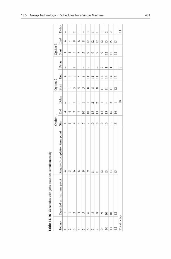
Table
13.16
Scheduleswithjobsexecutedsimultaneously
Jobno.
Expectedarrival
timepoint
Required
completiontimepoint
Option1
Option2
Option3
Start
End
Delay
Start
End
Delay
Start
End
Delay
11
41
4–
14
–1
4–
21
51
4–
14
–1
4–
33
64
71
58
25
82
44
84
7–
58
–5
8–
55
97
10
15
8–
58
–
66
97
10
18
11
29
12
3
78
11
10
13
28
11
–9
12
1
88
11
10
13
28
11
–9
12
1
99
12
10
13
111
14
29
12
–
10
10
13
10
13
–11
14
112
15
2
11
10
13
13
16
311
14
112
15
2
12
12
15
13
16
112
15
–12
15
–
Totaldelay
10
811
13.5 Group Technology in Schedules for a Single Machine 431
of the processing of the batch at time point 4 jobs 3 and 4 are ready for loading, the
processing of which is over by the time 7; similarly, jobs 5 and 6 are ready.
In the above cases, the number of possible jobs at the time of machine availabil-
ity was less than the machine capacity. By time 10 jobs 7, 8, 9, 10, and 11 will be
available for processing, i.e. the number of possible jobs exceeds machine capacity
b ¼ 4. In this case, the load batch should include only the first four jobs in order of
increasing required due time point. It is obvious that remaining jobs 11 and 12 must
make the last load batch.
For each of the schedule jobs, the value of planned delay is defined as the
difference between the time point of processing completion and the required due
time point. For example, for the above first option of the schedule, the total planned
delay in units of time scheduling is 10.
In order to reduce this delay the machine filling should be increased by enlarge-
ment of some load batch. According to the described algorithm, this can be done by
delaying loading, e.g. of jobs 3 and 4, in order to combine them with job 5 (option
2). By sequential load batching according to this option, we see that in this case, the
total delay is 8 units.
This process can be continued if, for example, in the schedule of option 2 the
loading of jobs 6, 7, and 8 is postponed by a unit in order to combine them with job
9 (option 3). However, scheduling under option 3 gives total delay of 11, which
obviously does not make sense. It is also possible to delay jobs 9, 10, and 11 by a
time unit and combine them with job 12; however, it is also impractical. Thus, in
this case, option 2 can be considered to be optimal.
13.5.3 Group Scheduling for Parallel Batches with MaximumAverage Utility Criterion
In actual practice of job assignments for the machine with simultaneous processing
multiple jobs, the list of these jobs is usually set with a small horizon, but the assign-
ments often include the jobs belonging to several different technological groups. For
such problems, it makes sense to use the branch-and-bound method with criterion of
average current utility maximum V described in above Sect. 2.6.2. In this case, the
classification formula is
1 batch;Cbatchð Þ��g��V ð13:21Þwhere parameter g indicates that the number of job groups requiring different process
settings can be any. The application of the relevant algorithm will be discussed in
terms of the input data in Table 13.17.
The data in Table 13.17 are compiled with a horizon of three working shifts
(24 h). Suppose also that occupied machine capacity in litres b ¼ 100, the setup
time for a load batch of any technological group is inconsiderable, the importance
of all jobs is the same and the machine is free at time 0. The arrival time, equalling
432 13 Shop Floor Scheduling: Single-Stage Problems
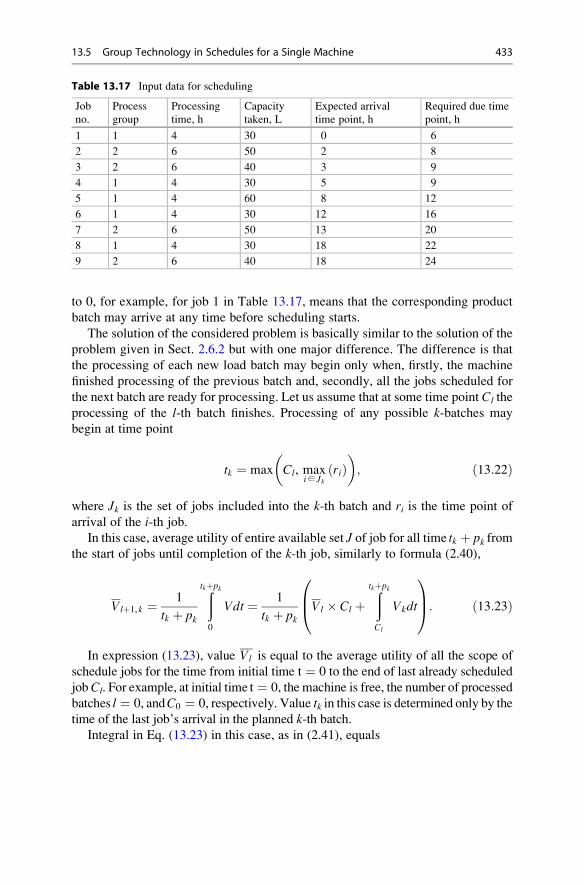
to 0, for example, for job 1 in Table 13.17, means that the corresponding product
batch may arrive at any time before scheduling starts.
The solution of the considered problem is basically similar to the solution of the
problem given in Sect. 2.6.2 but with one major difference. The difference is that
the processing of each new load batch may begin only when, firstly, the machine
finished processing of the previous batch and, secondly, all the jobs scheduled for
the next batch are ready for processing. Let us assume that at some time point Cl the
processing of the l-th batch finishes. Processing of any possible k-batches may
begin at time point
tk ¼ max Cl, maxi∈ Jk
rið Þ� �
; ð13:22Þ
where Jk is the set of jobs included into the k-th batch and ri is the time point of
arrival of the i-th job.
In this case, average utility of entire available set J of job for all time tk þ pk fromthe start of jobs until completion of the k-th job, similarly to formula (2.40),
Vlþ1,k ¼ 1
tk þ pk
ðtkþpk
0
Vdt ¼ 1
tk þ pkVl � Cl þ
ðtkþpk
Cl
Vkdt
0B@1CA: ð13:23Þ
In expression (13.23), value Vl is equal to the average utility of all the scope of
schedule jobs for the time from initial time t ¼ 0 to the end of last already scheduled
jobCl. For example, at initial time t ¼ 0, the machine is free, the number of processed
batches l ¼ 0, andC0 ¼ 0, respectively. Value tk in this case is determined only by the
time of the last job’s arrival in the planned k-th batch.Integral in Eq. (13.23) in this case, as in (2.41), equals
Table 13.17 Input data for scheduling
Job
no.
Process
group
Processing
time, h
Capacity
taken, L
Expected arrival
time point, h
Required due time
point, h
1 1 4 30 0 6
2 2 6 50 2 8
3 2 6 40 3 9
4 1 4 30 5 9
5 1 4 60 8 12
6 1 4 30 12 16
7 2 6 50 13 20
8 1 4 30 18 22
9 2 6 40 18 24
13.5 Group Technology in Schedules for a Single Machine 433
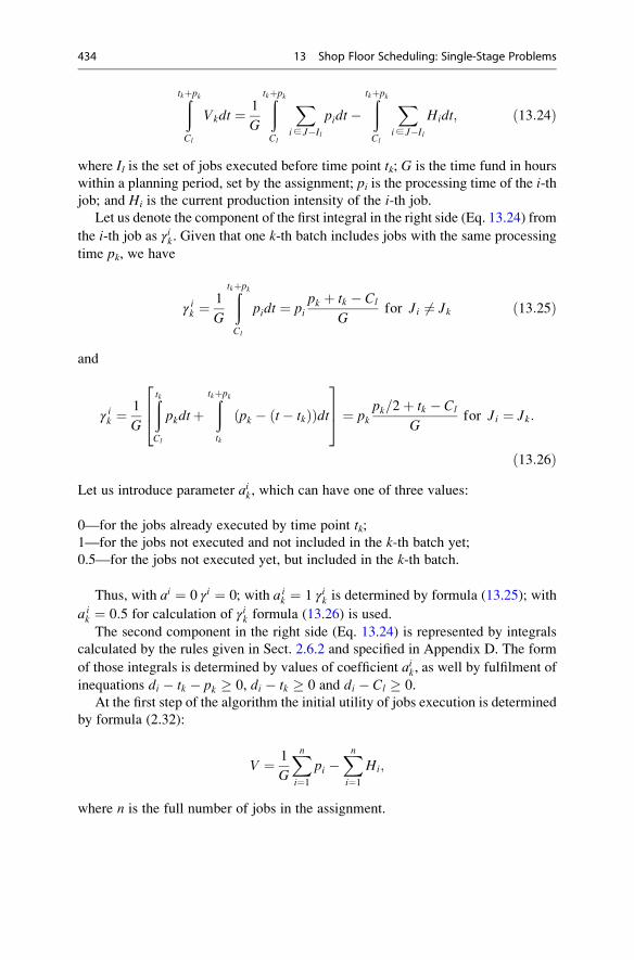
ðtkþpk
Cl
Vkdt ¼ 1
G
ðtkþpk
Cl
Xi∈ J�Il
pidt�ðtkþpk
Cl
Xi∈ J�Il
Hidt; ð13:24Þ
where Il is the set of jobs executed before time point tk; G is the time fund in hours
within a planning period, set by the assignment; pi is the processing time of the i-thjob; and Hi is the current production intensity of the i-th job.
Let us denote the component of the first integral in the right side (Eq. 13.24) from
the i-th job as γik. Given that one k-th batch includes jobs with the same processing
time pk, we have
γ ik ¼1
G
ðtkþpk
Cl
pidt ¼ pipk þ tk � Cl
Gfor Ji 6¼ Jk ð13:25Þ
and
γ ik ¼1
G
ðtkCl
pkdtþðtkþpk
tk
pk � t� tkð Þð Þdt
264375 ¼ pk
pk=2þ tk � Cl
Gfor Ji ¼ Jk:
ð13:26ÞLet us introduce parameter aik, which can have one of three values:
0—for the jobs already executed by time point tk;1—for the jobs not executed and not included in the k-th batch yet;
0.5—for the jobs not executed yet, but included in the k-th batch.
Thus, with ai ¼ 0 γi ¼ 0; with aik ¼ 1 γik is determined by formula (13.25); with
aik ¼ 0:5 for calculation of γik formula (13.26) is used.
The second component in the right side (Eq. 13.24) is represented by integrals
calculated by the rules given in Sect. 2.6.2 and specified in Appendix D. The form
of those integrals is determined by values of coefficient aik, as well by fulfilment of
inequations di � tk � pk � 0, di � tk � 0 and di � Cl � 0.
At the first step of the algorithm the initial utility of jobs execution is determined
by formula (2.32):
V ¼ 1
G
Xni¼1
pi �Xni¼1
Hi;
where n is the full number of jobs in the assignment.
434 13 Shop Floor Scheduling: Single-Stage Problems

In this case,n ¼ 9,G ¼ 24, values pi are given in Table 13.17. Since the requireddue date of any job has not yet passed, for all the jobs at the initial time, the intensity
may be determined by the first out of formulas (2.28), namely
Hi ¼ piG
1
di � tð Þ=αGþ 1:
Let us assume that like in examples of Chap. 2, psychological coefficient α ¼ 0:1.In this case at time t ¼ 0, for example for job 1, we have
H1 ¼ 4
24
1
6� 0ð Þ= 0:1� 24ð Þ þ 1¼ 0:047:
By determining the initial intensities for all jobsXni¼1
Hi ¼ 0:31, we obtain the value
of initial utility
V0 ¼ 44
24� 0:31 ¼ 1:52:
At the second step, it is necessary to identify possible load batches in each of two
technological groups, the total capacity of which does not exceed the machine capacity
in use. These batches are sets consisting of jobs {1}, {2}, {1, 4}, {2, 3}, {1, 4, 6}. These
sets are the nodes of the first level of the tree of searching for optimal solution that is
built starting from the initial stage of jobs execution (Fig. 13.7). The average utility will
be calculated using Table 13.18.
For example, in node 1, located on level 1, the set of planned jobs
Jk ¼ J1 ¼ 1f g. Previous level l ¼ 0 (Fig. 13.7) and the time of job completion at
this level C0 ¼ 0, respectively. The time point of arrival of the only job 1 in set
J1 ¼ 1f g, according to Table 13.17, is r1 ¼ 0. That is why job start time
tk¼ t1¼max Cl,maxi∈Jk
rið Þ� �
¼max 0,maxi∈J1
r1ð Þ� �
¼0. For job 1 in node 1, according
to formula (13.25), parameter value γ11¼p1p1=2þt1�C0
G ¼44=2þ0�0
24¼0:33.
Let us determine the component of average utility in this node from job 2. Since
this job is not included in the planned set, then a21 ¼ 1 and parameter
γ21 ¼ p2p1þt1�C0
G ¼ 6 4þ0�024
¼ 1. For job 2 in node 1, we have the following values
of parameters di� tk�pk ¼ d2� t1�p1¼ 8�0�4¼ 4; di� tk ¼ d2� t1¼ 8�0¼ 8;
di�Cl¼ 8�0¼ 8.
By the values of parameters a21, d2 � t1 � p1, d2 � t1 и di � Cl in Appendix 4 for
determining the production intensity, we select formula 1, using which we find
H21 ¼ 0:291. The value of average utility of job 2 in node 1, according to expressions
13.5 Group Technology in Schedules for a Single Machine 435
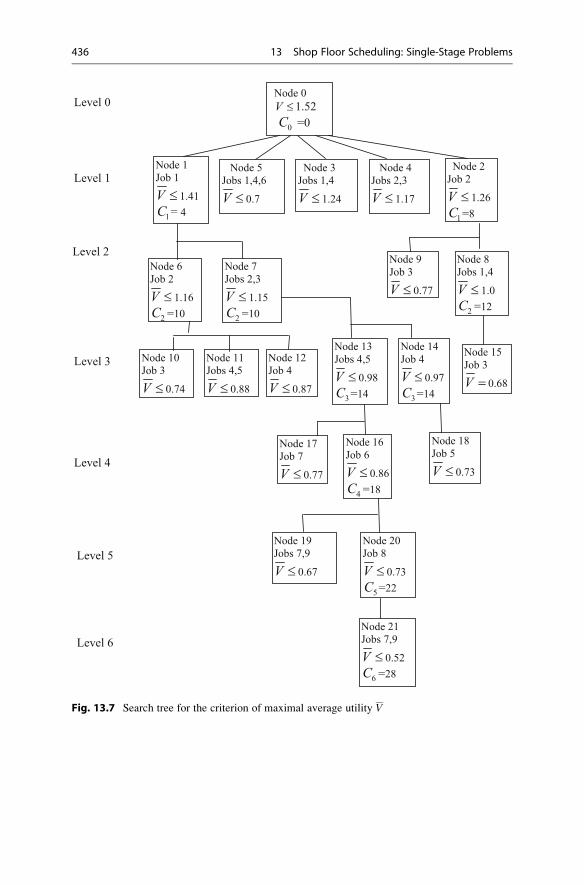
Fig. 13.7 Search tree for the criterion of maximal average utility V
436 13 Shop Floor Scheduling: Single-Stage Problems

Table
13.18
Calculationofaverageutility
fornodes
ofthesearchingtree
Level
lþ1;
Set
I l
Nodek;
composition;
start;
pk
Jobi
ai k
γi kdi�t k�p k
di�t k
di�Cl
Number
ofform
ula
forH
i kH
i kV
i k
l¼
0
I 0¼
fgC0¼
0
V0¼
0
k¼
1
J 1¼
1 fg
t 1¼
0
p1¼
4
10.5
0.33
26
62
0.115
0.05
21
14
88
10.291
0.18
31
15
99
10.259
0.19
41
0.67
59
91
0.173
0.12
51
0.67
812
12
10.13
0.13
61
0.67
12
16
16
10.098
0.14
71
116
20
20
10.118
0.22
81
0.67
18
22
22
10.072
0.15
91
120
24
24
10.099
0.23
Averageutility
innode1at
level
1V1,1¼
1:41
1.41
k¼
2
J 2¼
2 fg
t 2¼
2
p2¼
6
11
1.33
�24
61
0.973
0.05
20.5
1.25
06
82
0.427
0.09
...
91
216
22
24
10.217
0.22
Averageutility
innode2at
level
1V1,2¼
1:26
1.26
k¼
3
J 3¼
1;4
fg
t 3¼
5
p3¼
4
10.5
1.17
�31
64
0.75
0.04
21
2.25
�13
83
1.182
0.12
31
2.25
04
91
0.935
0.15
40.5
1.17
04
92
0.396
0.09
...
91
2.25
15
19
24
10.25
0.22
Averageutility
innode3at
level
1V1,3¼
1:24
1.24
(continued)
13.5 Group Technology in Schedules for a Single Machine 437
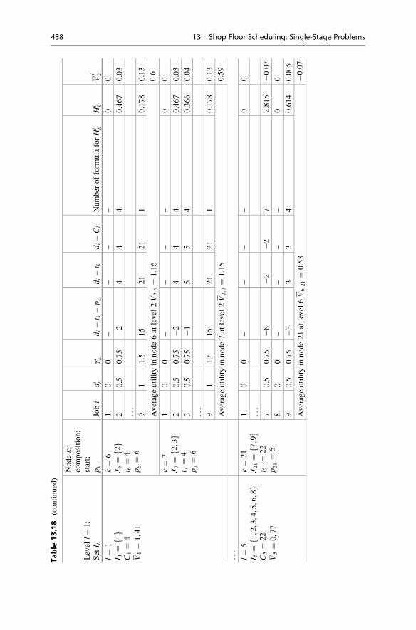
Table
13.18
(continued)
Level
lþ1;
Set
I l
Nodek;
composition;
start;
pk
Jobi
ai k
γi kdi�t k�p k
di�t k
di�Cl
Number
ofform
ula
forH
i kH
i kV
i k
l¼
1
I 1¼
1 fg
C1¼
4
V1¼
1,41
k¼
6
J 6¼
2 fg
t 6¼
4
p6¼
6
10
0–
––
–0
0
20.5
0.75
�24
44
0.467
0.03
...
91
1.5
15
21
21
10.178
0.13
Averageutility
innode6at
level
2V2,6¼
1:16
0.6
k¼
7
J 7¼
2;3
fg
t 7¼
4
p7¼
6
10
0–
––
–0
0
20.5
0.75
�24
44
0.467
0.03
30.5
0.75
�15
54
0.366
0.04
...
91
1.5
15
21
21
10.178
0.13
Averageutility
innode7at
level
2V2,7¼
1:15
0.59
...
l¼
5
I 5¼
1;2;3;4;5;6;8
fg
C5¼
22
V5¼
0,77
k¼
21
J 21¼
7;9
fg
t 21¼
22
p21¼
6
10
0–
––
–0
0
...
70.5
0.75
�8�2
�27
2.815
�0.07
80
0–
––
–0
0
90.5
0.75
�33
34
0.614
0.005
Averageutility
innode21at
level
6V6,21¼
0:53
�0.07
438 13 Shop Floor Scheduling: Single-Stage Problems
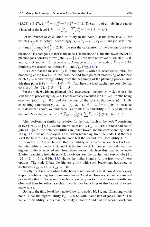
(13.24)–(13.27), is V2
1 ¼ γ21�H2
1
t1þp1¼ 1�0:291
0þ4¼ 0:18. The utility of all jobs in the node
1 located at the level 1, V1,1 ¼ VlCl
tkþpkþXi
Vik ¼ 0 ¼ 1:41 ¼ 1:41.
Let us transfer to calculation of utility in the node 2 at the same level 1, for
which C0 ¼ 0 as before. Accordingly, Jk ¼ J2 ¼ 2f g, r2 ¼ 2 and job start time
t2 ¼ max 0, maxi∈ J2
r2ð Þ� �
¼ 2. For the rest the calculation of the average utility in
the node 2 is analogous to that in the node 1. In the node 3 at the first level, the set of
planned jobs consists of two jobs J3 ¼ 1; 4f g, the time of arrival of which r1 ¼ 0,
and r4 ¼ 5 and t3 ¼ 5, respectively. Average utility in the node 3 V1,3 is 1.24.
Similarly we determine utilities V1,4 and V1,5 (Fig. 13.7).
It is clear that the most utility is in the node 1, which is accepted as initial for
branching at the level 2. In this case the end time point of processing of the first
batch C1 ¼ 4 and average utility from the beginning of the planning process until
this time point is Vl ¼ V1 ¼ 1:41 ¼ V1. And here the load batches are possible that
consist of jobs {2}, {2, 3}, {4}, {4, 5}.
For the node 6 with one planned job 2, received at time point r2 ¼ 2, the possible
start time of processing is t6 ¼ 4. For the already executed job 1a1 ¼ 0, for the being
executed job 2 a26 ¼ 0:5, and for the rest of the jobs in this node ai6 ¼ 1. By
calculating parameters γik, di � tk � pk, di � tk, di � Cl for all jobs in the node
6, as described above, we find the values of intensity and utility. Utility of all jobs in
the node 6 located at the level 2, V2,6 ¼ VlCl
tkþpkþXi
Vik ¼ 1:41�4
4þ6þ 0:6 ¼ 1:16.
After performing similar calculation for the load batch in the node 7 consisting
of two jobs J7 ¼ 2; 3f g, we find the value of utilityV2,7 ¼ 1:15. For load batches ofjobs {4}, {4, 5} the obtained utilities are much lower, and the corresponding nodes
in Fig. 13.7 are not displayed. Thus, when branching from the node 1 at the first
level the best result is given by the node 6 at the second level with utility 1.16.
From Fig. 13.7 it can be seen that such utility value on the second level is lower
than the utility in nodes 2, 3, and 4 at the first level. Of course, the node with the
highest utility is selected first from these nodes, which in this case is the node
2. After branching from the node 2, we obtain possible batches with sets of jobs {1},
{3}, {4}, {4, 5} and Fig. 13.7 shows the nodes 8 and 9 for the first two of these
options. The node 8 has the highest utility with such branching, however, its
usefulness V2,8 ¼ 1:0 < V2,6 ¼ 1:16.Strictly speaking, according to the branch-and-boundmethod, now it is necessary
to perform branching from remaining nodes 3 and 4. However, it can be assumed
practically that, if for some branch successively on two levels worse results are
observed than for other branches, then further branching of this branch does not
make sense.
Going to the third level from node 6 we form nodes 10, 11, and 12, among which
node 11 has the highest utility V3,11 ¼ 0:88 with load batch of jobs 4 and 5. The
value of this utility is less than the utility in nodes 7 and 8 at the second level, and
13.5 Group Technology in Schedules for a Single Machine 439
therefore branching should be performed from them. As the utility is the highest in
node 7, then during branching from it, we create nodes 13 and 14 at the third level.
The utility of these nodes is greater than that of node 11 obtained when branching
from node 6. This shows that here node 7 at the second level is more preferable than
node 6, despite the fact that its utility is lower than in node 6.
Since the re-branching from the node at the second level has led to an increase in
the potential utility at the third level, then branching at the second level should be
continued. However, when branching from node 8 at the second level, we see that in
all of such nodes (in Fig. 13.7 only node 15 with the greatest utility is shown) the
utility is lower than that when branching from node 7. Therefore, further branching
from the nodes at the second level can be stopped. Eventually, node 13 with a load
batch consisting of jobs 4 and 5 has the highest utility at the third level.
When branching for the next levels, we obtain the solution of the problem
in which all nine jobs are divided into six load batches J1 ¼ 1f g, J2 ¼ 2; 3f g,J3 ¼ 4; 5f g, J4 ¼ 6f g, J5 ¼ 8f g, and J6 ¼ 7; 9f g, and all the jobs are planned to befinished by time C6 ¼ 28, which is not much longer than the required due time
point, equalling to 24.
Despite some awkwardness of the formulas for intensity given in Appendix D,
the algorithm described above is easily realized in MS Excel spreadsheet. Wherein
the specified formulas are placed in some cells, and then for each new dataset are
simply copied to perform calculations.
13.6 Parallel Machine Scheduling
The theory of schedules differentiates three options of jobs scheduling for several
parallel machines:
• Identical machines;
• Uniform machines with different capacities;
• Unrelated machines.
Usually in the optimization problems, the schedules for parallel machines use
either the criterion of theminimal totalmachine operation timeXj
Cj or themakespan
Cmax. The first case was described above in Sect. 2.5.2, as, for example, the so-called
problem of allocation; the second option is discussed below.
13.6.1 Identical Parallel Machine Scheduling
Let us consider the problem of scheduling by criterion of the makespan Cmax (Sect.
2.2.2). For this case, the classification formula of the problem has the form
440 13 Shop Floor Scheduling: Single-Stage Problems

P�� ��Cmax; ð13:27Þ
where P is the designation of identical parallel machines.
The paper (Sule 2007) describes the algorithm of this problem’s solution, which
is illustrated in terms of data in Table 13.19. The jobs in Table 13.19 are positioned
in order of descending processing time. Let the number of parallel machinesm ¼ 3.
Let us determine the minimal possible value
C*max ¼
1
m
Xni¼1
pi ¼1
3� 74 ¼ 24:7:
We assume that each of the machines is available for scheduling new jobs, if the
sum of the previously planned jobs for it is less than Cmax. The difference between
Cmax and total time of previously planned jobs at each step of scheduling is called
remaining cumulative time. We denote this value as τr.We attach the next job work in order of descending processing time to the j-th
machine, if the obtained here value τrj is greater than or equal to 0. In the case whenτrj becomes less than 0, you need to begin scheduling for the next machine. Finally,
if the next operation results in that is τrj less than 0 for each ofmmachines, the job is
attached to that of them, for which value τrj is maximum. The application of this
algorithm to the data in the example in Table 13.19 is shown in Table 13.20.
Scheduling begins with attachment of the longest job 6 to the machine, which is
considered to be the first (i.e. the most desirable for the job). Since after this attaching
the value of remaining cumulative time is sufficient, then we can also attach job 3 to
the machine.
Then, obviously, it is necessary to start scheduling for machine 2. Attachment of
jobs 7 and 4 to this machine gives remaining time τrj equal to 4.7, which is not
enough to attach jobs 1 following by value of processing time. Therefore, schedul-
ing for machine 3 begins, during which it is possible to attach jobs 1, 5, and 9.
For scheduling job 8 it is suggested to find that of the machines, for which τrj ismaximum—this machine is machine 2. Similarly, job 2 is attached to machine 3.
Table 13.19 List of orders
Order number 6 3 7 4 1 5 9 8 2
Processing time pi 13 11 10 10 8 8 6 5 3
Table 13.20 Attaching
the jobs to the parallel
identical machines
Machine 1 Machine 2 Machine 3
Job pi τr1 Job pi τr2 Job pi τr36 13 11.7 7 10 14.7 1 8 16.7
3 11 0.7 4 10 4.7 5 8 8.7
8 5 �0.3 9 6 2.7
2 3 �0.3
13.6 Parallel Machine Scheduling 441
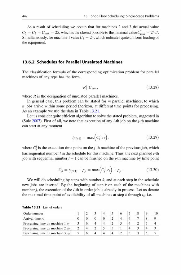
As a result of scheduling we obtain that for machines 2 and 3 the actual value
C2 ¼ C3 ¼ Cmax ¼ 25,which is the closest possible to theminimal valueC*max ¼ 24:7.
Simultaneously, formachine 1 valueC1 ¼ 24, which indicates quite uniform loading of
the equipment.
13.6.2 Schedules for Parallel Unrelated Machines
The classification formula of the corresponding optimization problem for parallel
machines of any type has the form
R�� ��Cmax; ð13:28Þ
where R is the designation of unrelated parallel machines.
In general case, this problem can be stated for m parallel machines, to which
n jobs arrive within some period (horizon) at different time points for processing.
As an example we use the data in Table 13.21.
Let us consider quite efficient algorithm to solve the stated problem, suggested in
(Sule 2007). First of all, we note that execution of any i-th job on the j-th machine
can start at any moment
tj lþ1ð Þ ¼ max Clj ; ri
� �; ð13:29Þ
where Clj is the execution time point on the j-th machine of the previous job, which
has sequential number l in the schedule for this machine. Thus, the next planned i-thjob with sequential number lþ 1 can be finished on the j-th machine by time point
Cji ¼ tj lþ1ð Þ þ pji ¼ max Clj ; ri
� �þ pji: ð13:30Þ
We will do scheduling by steps with number k, and at each step in the schedule
new jobs are inserted. By the beginning of step k on each of the machines with
number j, the execution of the l-th in order job is already in process. Let us denote
the maximal time point of availability of all machines at step k through tk, i.e.
Table 13.21 List of orders
Order number 1 2 3 4 5 6 7 8 9 10
Arrival time ri 0 0 0 0 2 4 4 7 8 9
Processing time on machine 1 pi1 3 6 4 4 2 3 4 2 5 4
Processing time on machine 2 pi2 2 4 2 5 5 1 4 3 4 3
Processing time on machine 3 pi3 5 6 4 4 4 2 3 3 5 5
442 13 Shop Floor Scheduling: Single-Stage Problems
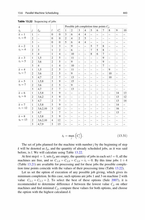
tk ¼ maxj
C lj
� �: ð13:31Þ
The set of jobs planned for the machine with number j by the beginning of step
k will be denoted as Ijk, and the quantity of already scheduled jobs, as it was said
before, is l. We will calculate using Table 13.22.
At first step k ¼ 1, sets Ijk are empty, the quantity of jobs in each set l ¼ 0, all the
machines are free, and so C1,0 ¼ C2,0 ¼ C3,0 ¼ t1 ¼ 0. By this time jobs 1� 4
(Table 13.21) are available for processing and for these jobs the possible comple-
tion time points coincide with the values of their processing time (Table 13.22).
Let us set the option of execution of any possible job giving, which gives its
minimum completion. In this case, such options are jobs 1 and 3 on machine 2 with
value C2,1 ¼ C2,3 ¼ 2. To select the best of these options (Sule 2007), it is
recommended to determine difference δ between the lowest value Cji on other
machines and find minimal Cji, compare these values for both options, and choose
the option with the highest calculated δ.
Table 13.22 Sequencing of jobs
ktk j Ijk l Cl
j
Possible job completion time points Cji
1 2 3 4 5 6 7 8 9 10
k ¼ 1
t1 ¼ 0
1 – 0 0 3 6 4 4 – – – – – –
2 – 0 0 2 4 2 5 – – – – – –
3 – 0 0 5 6 4 4 – – – – – –
k ¼ 2
t2 ¼ 4
1 1 1 3 – 9 – – 5 7 8 – – –
2 3 1 2 – 6 – – 7 5 8 – – –
3 4 1 4 – 10 – – 8 6 7 – – –
k ¼ 3
t3 ¼ 5
1 1,5 2 5 – 11 – – – – 9 – – –
2 3,6 2 5 – 9 – – – – 9 – – –
3 4 1 4 – 10 – – – – 7 – – –
k ¼ 4
t4 ¼ 7
1 1,5 2 5 – 11 – – – – – 9 – –
2 3,6 2 5 – 9 – – – – – 10 – –
3 4,7 2 7 – 13 – – – – – 10 – –
k ¼ 5
t5 ¼ 7
1 1,5,8 3 9 – 15 – – – – – – – –
2 3,6 2 5 – 9 – – – – – – – –
3 4,7 2 7 – 13 – – – – – – – –
k ¼ 6
t6 ¼ 6
1 1,5,8 3 9 – – – – – – – – 14 13
2 3,6,2 3 9 – – – – – – – – 13 12
3 4,7 2 7 – – – – – – – – 13 14
k ¼ 7
t7 ¼ 12
1 1,5,8 3 9 – – – – – – – – 14 –
2 3,6,2,10 3 12 – – – – – – – – 16 –
3 4,7 3 7 – – – – – – – – 13 –
k ¼ 8
t8 ¼ 13
1 1,5,8 3 9 – – – – – – – – – –
2 3,6,2,10 4 12 – – – – – – – – – –
3 4,7,9 3 13 – – – – – – – – – –
13.6 Parallel Machine Scheduling 443
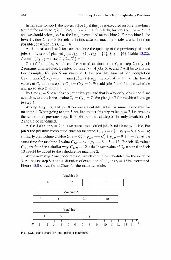
In this case for job 1, the lowest valueCji if this job is executed on other machines
(except for machine 2) is 3. So δ1 ¼ 3� 2 ¼ 1. Similarly, for job 3 δ3 ¼ 4� 2 ¼ 2
and we should select job 3 as the first job executed on machine 2. For machine 1, the
lowest value C1,1 ¼ 3 for job 1. In this case for machine 3 jobs 2 and 4 remain
possible, of which less C3,4 ¼ 4.
At the next step k ¼ 2 for each machine the quantity of the previously planned
jobs l ¼ 1, sets of planned jobs I1,2 ¼ 1f g, I2,2 ¼ 3f g, I3,2 ¼ 4f g (Table 13.22).
Accordingly, t2 ¼ max C11;C
12;C
13
� ¼ 4.
Out of four jobs, which can be started at time point 0, at step 2 only job
2 remains unscheduled. Besides, by time t2 ¼ 4 jobs 5, 6, and 7 will be available.
For example, for job 6 on machine 1 the possible time of job completion
C1,6 ¼ max C11; r6
� þ p1,6 ¼ max C1
1; r6� þ p
1,6 ¼ max 3; 4ð Þ þ 3 ¼ 7. The lowest
values of Cji at this step are C1,5 ¼ C2,6 ¼ 5. We add jobs 5 and 6 to the schedule
and go to step 3 with t3 ¼ 5.
By time t3 ¼ 5 new jobs do not arrive yet, and that is why only jobs 2 and 7 are
available, and the lowest valueCji ¼ C3,7 ¼ 7. We plan job 7 for machine 3 and go
to step 4.
At step 4 t4 ¼ 7, and job 8 becomes available, which is more reasonable for
machine 1. When going to step 5, we find that at this step value t5 ¼ 7, i.e. remains
the same as at previous step. It is obvious that at step 5 the only available job
2 should be scheduled.
At the sixth step t6 ¼ 9and twomore unscheduled jobs 9 and 10 are available. For
job 9 the possible completion time on machine 1 C1,9 ¼ C31 þ p1,9 ¼ 9þ 5 ¼ 14;
similarly on machine 2 value C2,9 ¼ Clj þ p2,9 ¼¼ C3
2 þ p2,9 ¼ 9þ 4 ¼ 13. At the
same time for machine 3 value C3,9 ¼ r9 þ p3,9 ¼ 8þ 5 ¼ 13. For job 10, values
Cj,10 are found in a similar way.C2,10 ¼ 12 is the lowest value ofCji at step 6 and job
10 should be added to the schedule for machine 2.
At the next step 7 one job 9 remains which should be scheduled for the machine
3. At the last step 8 the total duration of execution of all jobs t8 ¼ 13 is determined.
Figure 13.8 shows Gantt Chart for the made schedule.
1 2 3 4 5 6 7 8 9 10 11 12 13 14t
1 5 8
3 6 2 10
4 7 9
Machine 1
Machine 2
0
Machine 3
Fig. 13.8 Gantt chart for three parallel machines
444 13 Shop Floor Scheduling: Single-Stage Problems

References
Baker, K. R., & Trietsch, D. (2009). Principles of sequencing and scheduling. New York: Wiley.
Carlier, J. (1982). The one machine sequencing problem. European Journal of OperationalResearch, 11, 42–47.
Dobson, G. (1987). The economic lot-scheduling problem: Achieving feasibility using time-
varying lot sizes. Operations Research, 35, 764–771.Lawler, E. L. (1973). Optimal sequencing of a single machine subject to precedence constraints.
Management Science, 19, 544–546.Pinedo, M. L. (2005). Planning and scheduling in manufacturing and services. Berlin: Springer.Potts, C. N., & Kovalyov, M. Y. (2000). Scheduling with batching: A review. European Journal of
Operational Research, 120, 228–249.Sule, D. R. (2007). Production planning and industrial scheduling. London: Taylor & Francis
Group.
Tanayev, V. S., Kovalyov, M. Y., & Shafransky, Y. M. (1998). Theory of schedules. Grouptechnologies. Minsk: Institute of Technical Cybernetics, National Academy of Sciences of
Belarus (in Russian).
References 445
Shop Floor Scheduling: Multi-stageProblems 14
14.1 Synchronized Flowshop Production
This definition applies to three main types of production referred to in Sect. 1.3.1:
automated line (type 3a), versatile transfer line that produces only core products
(type 3b), and versatile transfer line that produces both core and by-products (type
3c). The main planning parameters of these kinds of repetitive production lines
are cycle, rhythm, number of jobs, as well as the size of stock (cycle stock) in the
buffers between the machines.
The cycle of repetitive line τ is the time between launches of two adjacent
objects (work pieces, materials, raw materials) or outputs from the repetitive line of
two adjacent finished products. In cases where the transfer from operation to
operation is carried out by transfer quantities, the rhythm of production line is
calculated.
R ¼ Qτ; ð14:1Þwhere Q is the quantity of the transfer lot.
To provide a unified cycle or rhythm for the repetitive production line it is
synchronized, meaning achievement of equality or multiplicity of the time of
individual operations of the process to the established rate. Typically, synchroniza-
tion is performed in two stages. Pre-synchronization with deviation from the cycle
time within 10 % is performed during engineering of the production line and final
synchronization—during its adjustment.
Full synchronization at all stages of processing is difficult to achieve because it is
required to have stepless adjustment of the processing time at each operation. So
actually, there is a situation in which the rhythm of the production line is defined by
duration of the longest operation and the machines occupied with other operations,
are idle for a while. We can suggest to consider the repetitive production to be
synchronized, if such idling does not exceed 10 % of the rhythm time. Discussion of
the synchronization methods is beyond the scope of this book.
# Springer International Publishing Switzerland 2016
Y. Mauergauz, Advanced Planning and Scheduling in Manufacturing and SupplyChains, DOI 10.1007/978-3-319-27523-9_14
447
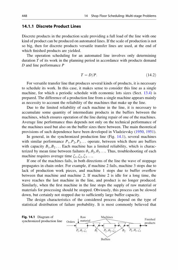
14.1.1 Discrete Product Lines
Discrete products in the production scale providing a full load of the line with one
kind of product can be produced on automated lines. If the scale of production is not
so big, then for discrete products versatile transfer lines are used, at the end of
which finished products are yielded.
The operation scheduling for an automated line involves only determining
duration T of its work in the planning period in accordance with products demand
D and line performance P
T ¼ D=P: ð14:2ÞFor versatile transfer line that produces several kinds of products, it is necessary
to schedule its work. In this case, it makes sense to consider this line as a single
machine, for which a periodic schedule with economic lots sizes (Sect. 13.4) is
prepared. The difference of a production line from a single machine appears mainly
as necessity to account the reliability of the machines that make up the line.
Due to the limited reliability of each machine in the line, it is necessary to
accumulate some quantity of intermediate products in the buffers between the
machines, which ensures operation of the line during repair of one of the machines.
Average line performance thus depends not only on the technical performance of
the machines used but also on the buffer sizes there between. The main theoretical
provisions of such dependence have been developed in Vladzievsky (1950, 1951).
In general, in the synchronized production line (Fig. 14.1), several machines
with similar performance P1,P2,P3 . . . operate, between which there are buffers
with capacity B1,B2 . . . Each machine has a limited reliability, which is charac-
terized by mean time between failures θ1, θ2, θ3 . . .. Thus, troubleshooting of each
machine requires average time ζ1, ζ2, ζ3 . . ..If one of the machines fails, in both directions of the line the wave of stoppage
propagates in chain order. For example, if machine 2 fails, machine 3 stops due to
lack of production work pieces, and machine 1 stops due to buffer overflow
between that machine and machine 2. If machine 2 is idle for a long time, the
wave reaches the last machine in the line, and product is no longer produced.
Similarly, when the first machine in the line stops the supply of raw material or
materials for processing should be stopped. Obviously, this process can be slowed
down, but certainly not stopped due to sufficiently large buffer capacity.
The design characteristics of the considered process depend on the type of
statistical distribution of failure probability. It is most commonly believed that
2B1B 3P , 3θ , 3ζ2P , 2θ , 2ζ1P , 1θ , 1ζ
OrdersFinished products
Raw material
Buffers
MachinesFig. 14.1 Diagram of
synchronized production line
448 14 Shop Floor Scheduling: Multi-stage Problems
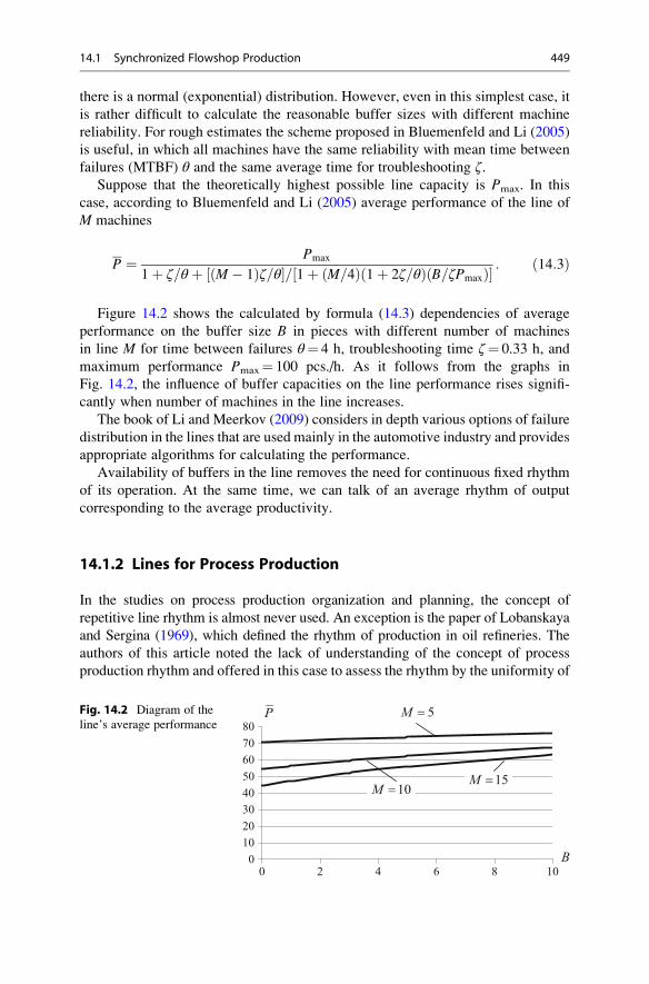
there is a normal (exponential) distribution. However, even in this simplest case, it
is rather difficult to calculate the reasonable buffer sizes with different machine
reliability. For rough estimates the scheme proposed in Bluemenfeld and Li (2005)
is useful, in which all machines have the same reliability with mean time between
failures (MTBF) θ and the same average time for troubleshooting ζ.Suppose that the theoretically highest possible line capacity is Pmax. In this
case, according to Bluemenfeld and Li (2005) average performance of the line of
M machines
P ¼ Pmax
1þ ζ=θ þ M � 1ð Þζ=θ½ �= 1þ M=4ð Þ 1þ 2ζ=θð Þ B=ζPmaxð Þ½ � : ð14:3Þ
Figure 14.2 shows the calculated by formula (14.3) dependencies of average
performance on the buffer size B in pieces with different number of machines
in line M for time between failures θ¼ 4 h, troubleshooting time ζ¼ 0.33 h, and
maximum performance Pmax¼ 100 pcs./h. As it follows from the graphs in
Fig. 14.2, the influence of buffer capacities on the line performance rises signifi-
cantly when number of machines in the line increases.
The book of Li and Meerkov (2009) considers in depth various options of failure
distribution in the lines that are used mainly in the automotive industry and provides
appropriate algorithms for calculating the performance.
Availability of buffers in the line removes the need for continuous fixed rhythm
of its operation. At the same time, we can talk of an average rhythm of output
corresponding to the average productivity.
14.1.2 Lines for Process Production
In the studies on process production organization and planning, the concept of
repetitive line rhythm is almost never used. An exception is the paper of Lobanskaya
and Sergina (1969), which defined the rhythm of production in oil refineries. The
authors of this article noted the lack of understanding of the concept of process
production rhythm and offered in this case to assess the rhythm by the uniformity of
0
10
20
30
40
50
60
70
80
0 2 4 6 8 10
10M =
5M =P
B
15M =
Fig. 14.2 Diagram of the
line’s average performance
14.1 Synchronized Flowshop Production 449
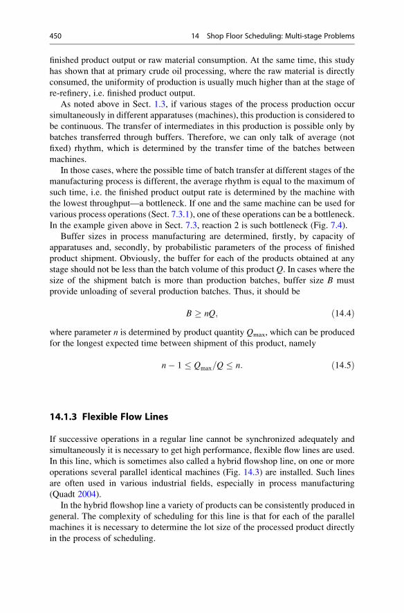
finished product output or raw material consumption. At the same time, this study
has shown that at primary crude oil processing, where the raw material is directly
consumed, the uniformity of production is usually much higher than at the stage of
re-refinery, i.e. finished product output.
As noted above in Sect. 1.3, if various stages of the process production occur
simultaneously in different apparatuses (machines), this production is considered to
be continuous. The transfer of intermediates in this production is possible only by
batches transferred through buffers. Therefore, we can only talk of average (not
fixed) rhythm, which is determined by the transfer time of the batches between
machines.
In those cases, where the possible time of batch transfer at different stages of the
manufacturing process is different, the average rhythm is equal to the maximum of
such time, i.e. the finished product output rate is determined by the machine with
the lowest throughput—a bottleneck. If one and the same machine can be used for
various process operations (Sect. 7.3.1), one of these operations can be a bottleneck.
In the example given above in Sect. 7.3, reaction 2 is such bottleneck (Fig. 7.4).
Buffer sizes in process manufacturing are determined, firstly, by capacity of
apparatuses and, secondly, by probabilistic parameters of the process of finished
product shipment. Obviously, the buffer for each of the products obtained at any
stage should not be less than the batch volume of this product Q. In cases where thesize of the shipment batch is more than production batches, buffer size B must
provide unloading of several production batches. Thus, it should be
B � nQ; ð14:4Þwhere parameter n is determined by product quantity Qmax, which can be produced
for the longest expected time between shipment of this product, namely
n� 1 � Qmax=Q � n: ð14:5Þ
14.1.3 Flexible Flow Lines
If successive operations in a regular line cannot be synchronized adequately and
simultaneously it is necessary to get high performance, flexible flow lines are used.
In this line, which is sometimes also called a hybrid flowshop line, on one or more
operations several parallel identical machines (Fig. 14.3) are installed. Such lines
are often used in various industrial fields, especially in process manufacturing
(Quadt 2004).
In the hybrid flowshop line a variety of products can be consistently produced in
general. The complexity of scheduling for this line is that for each of the parallel
machines it is necessary to determine the lot size of the processed product directly
in the process of scheduling.
450 14 Shop Floor Scheduling: Multi-stage Problems
A detailed study of this problem for discrete manufacturing is given in Quadt
(2004), and the problem is solved in three successive stages. At the first stage, the
planning is done for a group of machines performing the operation, which is the
bottleneck of the process. At the second stage, based on the results of the first stage,
lot sizing and planning for the rest machines are carried out. As a result of the
second stage, the so-called machine/time slots are determined for each product by,
which show what time and on what machine each product to be processed.
The third step is required in those cases where one line produces several different
groups of similar products. In such cases, at the second stage the planning is made
by aggregate groups, and at the last stage the disaggregation of the plan for each
product group is confirmed.
As the objective function at the first stage minimization of direct costs is applied,
at the second stage—minimization of process time. During the third stage, the
changeover cost is minimized while maintaining quite short processing time.
For solution at the first stage, we use the methodology outlined above in
Sect. 11.1.3, for Capacitated Multi-Item Lot Sizing Problem (CLSP). To account
for the changeover duration for the i-th product si in the model described by
dependencies (11.5)–(11.9), constraint (11.9) is adjusted, which takes the form
Xni¼1
piXit þ siδit � Pt; ð14:6Þ
where Pt is understood as the total capacity in hours for a period of time t of allparallel machines on the operation being a bottleneck.
Since the optimal lot sizes of the products for each planning period are
established at the first stage of planning, i.e. by bottleneck capacity, at the second
stage we only need to perform the procedure of schedule roll-out for each operation
in accordance with its position in the process. As the number of parallel machines
on various operations is different, then in this procedure it is necessary to take into
account the changes in lot size at the same time.
2B1B
OrdersFinished products
Raw material
Buffers
Operation 1 Operation 3
Parallel machines
Operation 2
Operation 2
Operation 2
Fig. 14.3 Flexible flow line on one operation
14.1 Synchronized Flowshop Production 451

Description of various approaches to planning of hybrid workshop line operation
is contained in the review articles (Ribas et al. 2010; Ruiz and Vazquez-Rodrıguez
2010).
14.2 Automated Assembly Lines
The assembly line consists of a number of assembly stations along the conveyor
transporting the consistently assembled product. Assembly operations can be car-
ried out directly on the conveyor, and in this case, it is called a working conveyor. If
the object to be assembled is removed from the conveyor to perform the assembling
operation, and after the operation is returned to the conveyor, it is called a distri-
bution conveyor.
When assembling on the working conveyor all operators move within their work
areas and then return to its front end. Distribution conveyor enables the operator
to reside at his workplace. Moreover, the continuous motion of the distribution
conveyor is not required and this conveyor may be run periodically and thus moved
stepwise.
Depending on the number of types of products assembled on the line, and also on
the sequence of launching different types, the lines can be differentiated as single-
model line, multi-model line, and mixed-model line (Fig. 14.4).
Various geometric figures in Fig. 14.4 represent corresponding assemble products.
Mixed assembly of various products (Fig. 14.4b) can be used in cases where there is
no need for significant changeover from one product to another. Otherwise, it is
necessary to use the diagram shown in Fig. 14.4c, i.e. assemble the products of the
same type by lots.
During assembly, the full scope of assembly jobs is made of individual assembly
operations—tasks, which must be performed in a certain sequence. For each of
these tasks, the standard time for its fulfilment by a semiskilled operator is known.
When designing the assembly line the main problem is the correct distribution of
c)
b)
a)
Fig. 14.4 Diagram of assembly lines: (a) single-model line; (b) mixed-model line; (c) multi-
model line
452 14 Shop Floor Scheduling: Multi-stage Problems

operations between assembly stations, providing the so-called Assembly Line
Balancing Problem (ALBP).
Assembly lines are divided into paced assembly lines and unpaced assembly
lines. Balancing problem exists for both types of lines, but in the latter case, it is
also necessary to determine the correct location of the buffers between assembly
stations.
Assembly Line Balancing Problem is discussed in a large number of papers, the
analysis of which is given in the review (Becker and Scholl 2006). If adequate
balance of the assembly line is impossible, as well as for processing lines, some-
times parallel assembly stations are installed, i.e. hybrid workshop lines are used
(Sect. 14.1.3). Consideration of the problem of the assembly line synchronization,
as well as the similar problem of processing line synchronization in Sect. 14.1, is
beyond the scope of this book.
We note only that there is an option of assembly line operation, in which
so-called Self-Balancing Assembly Line may take place (Bartholdi and Eisenstein
1996). In this line, operators are located along it in ascending order of individual
possible speed of their work. In this case, each successive operator can undertake
the functions of the previous operator, if the latter cannot keep up the pace of the
line. Of course, for this purpose, the operators must be trained appropriately.
14.2.1 Scheduling for Unpaced Assembly Lines
Let us consider the scheduling of the assembly line with buffers between assembly
stations. If any of the buffers is full, then the previous station is forced to stop
working because it becomes blocked; if the buffer is empty, and at the previous
station the assembly is not finished yet, the work on the next station is ceased.
Therefore, in the single-model line, the line throughput is ultimately determined by
the station with the lowest throughput.
In operation of the line with mixed launching sequence for various products, the
situation depends on the launch sequence. It is obvious that planning should provide
such a launch sequence for assembly of various products that ensures minimal
downtime of the line.
If the demand for the products produced on the line is constant, it makes sense to
develop a cyclic-repeated schedule of these products output. Recurring schedule
greatly simplifies the supplying of the line with necessary materials and other
assembly elements.
Assume that l kinds of different products should be assembled on the line, and
the demand for the k-th product during a plan period, such as a month, is Dk. We
introduce the vector
D* ¼ D1
a,D2
a. . .
Dl
a
� �; ð14:7Þ
14.2 Automated Assembly Lines 453

for consideration with components Dk/a, where a is the most common divider. This
vector is represented by the smallest set of the assembled products having the same
proportions as many other products produced within the entire planning period.
This set is called Minimum Part Set (MPS), and the number of parts to be performed
in this set is equal to the total of the components of this set, i.e.
n ¼ 1
a
Xlk¼1
Dk: ð14:8Þ
If one makes an optimal assembly schedule for the minimal set, this schedule can
be repeated during the plan period and will be optimal. An optimality criterion is
usually the minimum duration of the assembly of all the parts in the minimal set.
Let us assume that the processing time of the i-th job on the j-th machine is pij.When scheduling for the minimal set, the processing time of some jobs can be
repeated if these jobs are an assembly of identical products.
As an example, we consider the assembly scheduling for the line with diagram
that is shown in Fig. 14.5. The line consists of three assembly stations 1, 3, 4, and
buffer 2 containing one assembling product. The line is designed for assembly of
several types of products, and the setup time from one type to another is assumed to
be inconsiderable, i.e. it is a mixed assembly line (Fig. 14.4b).
An effective algorithm of optimal scheduling for an unpaced assembly line is
suggested in the paper (McCormick et al. 1989) and is called “Profile Fitting” (PF).
The block diagram of the algorithm is shown in Fig. 14.6.
Let us consider the algorithm operation when scheduling for the line in Fig. 14.5,
which should collect the products of three types in quantity D1¼ 24 pcs./month,
D2 ¼ D3 ¼ 12 pcs./month. Since the most common divider of these values a¼ 12,
then by using formulas (14.7) and (14.8), we obtain the vector of minimal part set
D*¼ (2,1,1) and the number of part in the set n¼ 4. Table 14.1 shows the standards
of processing time of assembling different types of products on each of three
assembly stations.
In accordance with the block diagram in Fig. 14.6, first we find a job with the
highest total processing time, and in this case, job 1 can be considered as this kind of
jobs. Then (block 3), we consistently consider the practicability of including the rest
of the jobs into the schedule as the second job in order. To do this, we construct the
Gantt chart for the assembly line with every possible sequence option of two jobs
{1, 2}, {1, 3}, {1, 4}.
B =1
JobsFinished products
1 3 42
Assembly elements
Fig. 14.5 Diagram of
assembly line
454 14 Shop Floor Scheduling: Multi-stage Problems

For example, Fig. 14.7a shows the sequence option of jobs 1 and 2. When con-
structing, we initially believe that job 1 is performed without delays. If job 2 is
performed as the following in order, then at the second and third stations downtimes
of 1 h are unavoidable. Thus, the non-productive time of the line (block 4 in
Fig. 14.6) in this case is 2 h.
If after job 1 job 3 is performed (Fig. 14.7b), then after the first station job 3 can
be transferred to station 2 immediately. After assembling on station 2, however, job
3 should wait for station 3 to be freed from previous job 1, i.e. station 2 appears to
be blocked. In this case, the non-productive time of the line is 1 h.
When performing job 4 after job 1 (Fig. 14.7c) the assembly on the first station
finishes before the station 2 is free. However, in this case, job 4 can be moved into
the buffer, and accordingly, does not create non-productive time. Therefore, the
case of sequence {1, 4} is the best possible and should be recorded in the schedule
(blocks 6 and 7 in Fig. 14.6).
With continuing operation of the algorithm until the end (block 8), the sequence
for the minimum set becomes {1, 4, 3, 2}. Figure 14.8 shows this sequence for the
first cycle and a section of this sequence in the second cycle. Obviously, in this case
the average rhythm of the line can be understood as the assembly period of the
minimum set, i.e. the schedule cycle time, which is equal to 13 h.
Start
1. Selection of a job with the highest total processing time
3. Cycle for the jobs non-scheduled yet
2. Including the job into the schedule
8.Are all jobsscheduled?
5.End of cycle
End
6. Selection of a job with the shortest non-productive time
4. Calculation of the non-productive time of the line
Yes
No
No
Yes7. Including the job into the schedule
Fig. 14.6 Block diagram of Profile Fitting algorithm
Table 14.1 Time
standards on three
assembly stations
Product type 1 2 3
Job no. 1 2 3 4
pi1 4 4 3 2
pi2 3 3 2 3
pi3 3 3 3 2
14.2 Automated Assembly Lines 455
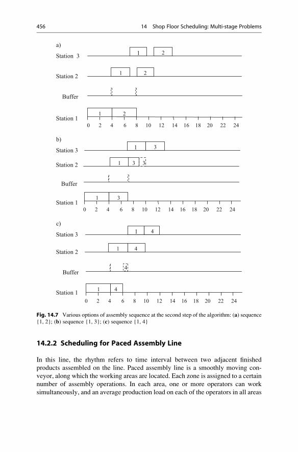
14.2.2 Scheduling for Paced Assembly Line
In this line, the rhythm refers to time interval between two adjacent finished
products assembled on the line. Paced assembly line is a smoothly moving con-
veyor, along which the working areas are located. Each zone is assigned to a certain
number of assembly operations. In each area, one or more operators can work
simultaneously, and an average production load on each of the operators in all areas
Station 3
Station 2
Buffer
Station 120 4 6 8 10 12 14 16 18 20 22 24
1
1
1
2
2
2
Station 3
Station 2
Buffer
Station 120 4 6 8 10 12 14 16 18 20 22 24
1
1
1
3
3
3
3
Station 3
Station 2
Buffer
Station 1
20 4 6 8 10 12 14 16 18 20 22 24
1
1
1
4
4
4
4
a)
b)
c)
Fig. 14.7 Various options of assembly sequence at the second step of the algorithm: (a) sequence{1, 2}; (b) sequence {1, 3}; (c) sequence {1, 4}
456 14 Shop Floor Scheduling: Multi-stage Problems
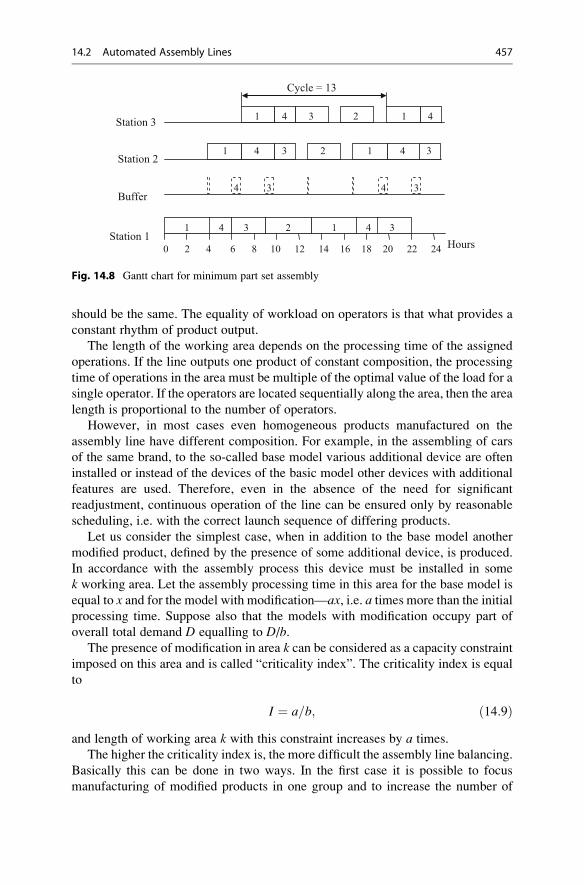
should be the same. The equality of workload on operators is that what provides a
constant rhythm of product output.
The length of the working area depends on the processing time of the assigned
operations. If the line outputs one product of constant composition, the processing
time of operations in the area must be multiple of the optimal value of the load for a
single operator. If the operators are located sequentially along the area, then the area
length is proportional to the number of operators.
However, in most cases even homogeneous products manufactured on the
assembly line have different composition. For example, in the assembling of cars
of the same brand, to the so-called base model various additional device are often
installed or instead of the devices of the basic model other devices with additional
features are used. Therefore, even in the absence of the need for significant
readjustment, continuous operation of the line can be ensured only by reasonable
scheduling, i.e. with the correct launch sequence of differing products.
Let us consider the simplest case, when in addition to the base model another
modified product, defined by the presence of some additional device, is produced.
In accordance with the assembly process this device must be installed in some
k working area. Let the assembly processing time in this area for the base model is
equal to x and for the model with modification—ax, i.e. a times more than the initial
processing time. Suppose also that the models with modification occupy part of
overall total demand D equalling to D/b.The presence of modification in area k can be considered as a capacity constraint
imposed on this area and is called “criticality index”. The criticality index is equal
to
I ¼ a=b; ð14:9Þand length of working area k with this constraint increases by a times.
The higher the criticality index is, the more difficult the assembly line balancing.
Basically this can be done in two ways. In the first case it is possible to focus
manufacturing of modified products in one group and to increase the number of
Cycle = 13
Station 3
Station 2
Buffer
Station 120 4 6 8 10 12 14 16 18 20 22 24
1
1
1
4
4
4
4
3
3
3
3
2
2
2
1
1
1
4 3
4 3
4 3
4
Hours
Fig. 14.8 Gantt chart for minimum part set assembly
14.2 Automated Assembly Lines 457
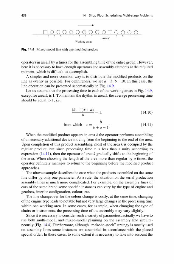
operators in area k by a times for the assembling time of the entire group. However,
here it is necessary to have enough operators and assembly elements at the required
moment, which is difficult to accomplish.
A simpler and more common way is to distribute the modified products on the
line as evenly as possible. For definiteness, we set a¼ 3; b¼ 10. In this case, the
line operation can be presented schematically in Fig. 14.9.
Let us assume that the processing time in each of the working areas in Fig. 14.9,
except for area k, is 1. To maintain the rhythm in area k, the average processing time
should be equal to 1, i.e.
b� 1ð Þxþ ax
b¼ 1; ð14:10Þ
from which x ¼ b
bþ a� 1: ð14:11Þ
When the modified product appears in area k the operator performs assembling
of a necessary additional device moving from the beginning to the end of the area.
Upon completion of this product assembling, most of the area k is occupied by the
regular product, but since processing time x is less than a unity according to
expression (14.11), then the operator of area k gradually shifts to the beginning of
the area. When choosing the length of the area more than regular by a times, the
operator definitely manages to return to the beginning before the modified product
approaches.
The above example describes the case when the products assembled on the same
line differ by only one parameter. As a rule, the situation on the serial production
assembly lines is much more complicated. For example, on the assembly lines of
cars of the same brand some specific instances can vary by the type of engine and
gearbox, interior configuration, colour, etc.
The line changeover for the colour change is costly; at the same time, changing
of the engine type leads to notable but not very large changes in the processing time
within one working area. In some cases, for example, when changing the type of
chairs or instruments, the processing time of the assembly may vary slightly.
Since it is necessary to consider such a variety of parameters, actually we have to
use both multi-model and mixed-model planning on the assembly line simulta-
neously (Fig. 14.4). Furthermore, although “make-to-stock” strategy is mostly used
on assembly lines some instances are assembled in accordance with the placed
special order. In these cases, to some extent it is necessary to take into account the
Working areas
Area k
Fig. 14.9 Mixed-model line with one modified product
458 14 Shop Floor Scheduling: Multi-stage Problems

shipping date specified in the order. Sometimes the date of shipment may also be
defined by the need to co-shipment of several instances of the product under the
terms of transportation.
It is not always possible to meet all these requirements at the same time and in
full. Therefore, usually in planning these requirements are ranked, i.e. some hierar-
chy is established: colour can be considered as a more important requirement,
the date of shipment often comes next, etc. The book (Pinedo 2005) presents the
algorithm of the type, which is called “Grouping and Spacing” developed for the
automotive industry.
At the first step, the algorithm sets the planning horizon and the number of
assembled products for which planning is carried out. This horizon is determined by
the scheduler’s experience as the time, during which significant fluctuations in the
requirements for line performance and assembled nomenclature are hardly proba-
ble. Typically, the value of the planning horizon is from 1 day to a working week.
At the second stage, the planned jobs are divided into groups to perform an
operation that requires significant expenditures on changeover. The duration of this
operation for each group depends mainly on the number of items in the group. If
some group appears to be much more than other groups, it can be divided into parts.
Such division slightly increases the cost of changeover, but can accelerate the
performance of individual controlled orders.
At the third step, the fulfilments of obtained groups is planned in such a way so
to fulfil given orders with smaller delay. In addition, as close as possible to these
orders those jobs are scheduled, which must be shipped together with important
orders.
Finally, at the last stage, the remaining jobs are distributed along the conveyor so
that various modifications of the basic configuration of the product were placed as
even as possible.
Let us consider the example (Table 14.2). Let us assume that within an 8-h shift
ten instances of the product different by colour and motor unit type are assembled.
The line cycle in this case is 0.8 h. Besides, jobs 2 and 9 must be shipped together
with desired shipping point 3 h after the operation start.
In this example, the planning horizon is set, and the jobs are divided into groups
with the same colour. In order to bring completion of job 9 into proximity to
the possible time of shipment together with job 2, first the assembly of products
with colour 3 should be scheduled, and then directly the assembly of products with
colour 1. Since out of total of 10 pieces two products (2 and 7) are assembled with
motor unit type 2, then for reasons of uniform assembly between jobs with type
2 four jobs with unit type 1 should be.
Table 14.2 Set of jobs in the line for scheduling
Job 1 2 3 4 5 6 7 8 9 10
Colour code 1 1 1 1 1 2 2 2 3 3
Engine unit type 1 2 1 1 1 1 2 1 1 1
Preferred shipping time point – 3 – – – – – – 3 –
14.2 Automated Assembly Lines 459
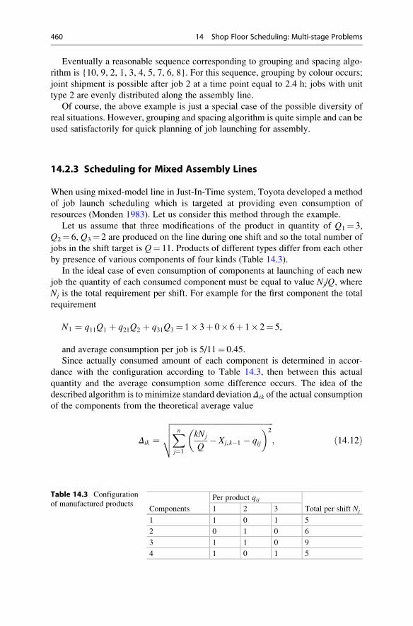
Eventually a reasonable sequence corresponding to grouping and spacing algo-
rithm is {10, 9, 2, 1, 3, 4, 5, 7, 6, 8}. For this sequence, grouping by colour occurs;
joint shipment is possible after job 2 at a time point equal to 2.4 h; jobs with unit
type 2 are evenly distributed along the assembly line.
Of course, the above example is just a special case of the possible diversity of
real situations. However, grouping and spacing algorithm is quite simple and can be
used satisfactorily for quick planning of job launching for assembly.
14.2.3 Scheduling for Mixed Assembly Lines
When using mixed-model line in Just-In-Time system, Toyota developed a method
of job launch scheduling which is targeted at providing even consumption of
resources (Monden 1983). Let us consider this method through the example.
Let us assume that three modifications of the product in quantity of Q1¼ 3,
Q2¼ 6, Q3¼ 2 are produced on the line during one shift and so the total number of
jobs in the shift target is Q¼ 11. Products of different types differ from each other
by presence of various components of four kinds (Table 14.3).
In the ideal case of even consumption of components at launching of each new
job the quantity of each consumed component must be equal to value Nj/Q, whereNj is the total requirement per shift. For example for the first component the total
requirement
N1 ¼ q11Q1 þ q21Q2 þ q31Q3 ¼ 1� 3þ 0� 6þ 1� 2¼ 5,
and average consumption per job is 5/11¼ 0.45.
Since actually consumed amount of each component is determined in accor-
dance with the configuration according to Table 14.3, then between this actual
quantity and the average consumption some difference occurs. The idea of the
described algorithm is to minimize standard deviation Δik of the actual consumption
of the components from the theoretical average value
Δik ¼ffiffiffiffiffiffiffiffiffiffiffiffiffiffiffiffiffiffiffiffiffiffiffiffiffiffiffiffiffiffiffiffiffiffiffiffiffiffiffiffiffiffiffiffiffiffiffiffiffiffiffiffiXnj¼1
kNj
Q� Xj,k�1 � qij
� �2vuut ; ð14:12Þ
Table 14.3 Configuration
of manufactured productsComponents
Per product qijTotal per shift Nj1 2 3
1 1 0 1 5
2 0 1 0 6
3 1 1 0 9
4 1 0 1 5
460 14 Shop Floor Scheduling: Multi-stage Problems
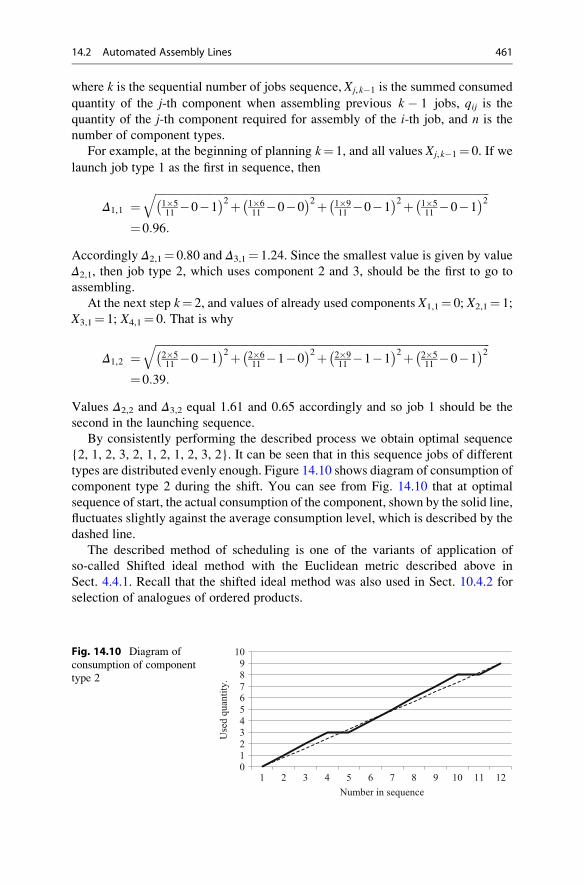
where k is the sequential number of jobs sequence, Xj,k�1 is the summed consumed
quantity of the j-th component when assembling previous k � 1 jobs, qij is the
quantity of the j-th component required for assembly of the i-th job, and n is the
number of component types.
For example, at the beginning of planning k¼ 1, and all values Xj,k�1¼ 0. If we
launch job type 1 as the first in sequence, then
Δ1,1 ¼ffiffiffiffiffiffiffiffiffiffiffiffiffiffiffiffiffiffiffiffiffiffiffiffiffiffiffiffiffiffiffiffiffiffiffiffiffiffiffiffiffiffiffiffiffiffiffiffiffiffiffiffiffiffiffiffiffiffiffiffiffiffiffiffiffiffiffiffiffiffiffiffiffiffiffiffiffiffiffiffiffiffiffiffiffiffiffiffiffiffiffiffiffiffiffiffiffiffiffiffiffiffiffiffiffiffiffiffiffiffiffiffiffiffiffiffiffiffiffiffiffi1�511
�0�1� 2þ 1�6
11�0�0
� 2þ 1�911
�0�1� 2þ 1�5
11�0�1
� 2q¼0:96:
Accordingly Δ2,1¼ 0.80 and Δ3,1¼ 1.24. Since the smallest value is given by value
Δ2,1, then job type 2, which uses component 2 and 3, should be the first to go to
assembling.
At the next step k¼ 2, and values of already used components X1,1¼ 0; X2,1¼ 1;
X3,1¼ 1; X4,1¼ 0. That is why
Δ1,2 ¼ffiffiffiffiffiffiffiffiffiffiffiffiffiffiffiffiffiffiffiffiffiffiffiffiffiffiffiffiffiffiffiffiffiffiffiffiffiffiffiffiffiffiffiffiffiffiffiffiffiffiffiffiffiffiffiffiffiffiffiffiffiffiffiffiffiffiffiffiffiffiffiffiffiffiffiffiffiffiffiffiffiffiffiffiffiffiffiffiffiffiffiffiffiffiffiffiffiffiffiffiffiffiffiffiffiffiffiffiffiffiffiffiffiffiffiffiffiffiffiffiffi2�511
�0�1� 2þ 2�6
11�1�0
� 2þ 2�911
�1�1� 2þ 2�5
11�0�1
� 2q¼0:39:
Values Δ2,2 and Δ3,2 equal 1.61 and 0.65 accordingly and so job 1 should be the
second in the launching sequence.
By consistently performing the described process we obtain optimal sequence
{2, 1, 2, 3, 2, 1, 2, 1, 2, 3, 2}. It can be seen that in this sequence jobs of different
types are distributed evenly enough. Figure 14.10 shows diagram of consumption of
component type 2 during the shift. You can see from Fig. 14.10 that at optimal
sequence of start, the actual consumption of the component, shown by the solid line,
fluctuates slightly against the average consumption level, which is described by the
dashed line.
The described method of scheduling is one of the variants of application of
so-called Shifted ideal method with the Euclidean metric described above in
Sect. 4.4.1. Recall that the shifted ideal method was also used in Sect. 10.4.2 for
selection of analogues of ordered products.
0123456789
10
1 2 3 4 5 6 7 8 9 10 11 12
Use
d q
uan
tity
.
Number in sequence
Fig. 14.10 Diagram of
consumption of component
type 2
14.2 Automated Assembly Lines 461
14.3 Unsynchronized Flowshop Production
When you synchronize a serial discrete production the full processing time of jobs
performed is divided into separate operations of short duration. This allows to
choose the set of operations, having about the same duration for each machine in
the line. Accordingly, the machine that performs these special operations usually
should also be specialized. Therefore, the cost of the line is a significant value, and
such lines can be used only in large-scale production.
If the scale of production is small, discrete products are manufactured on
widespread general-purpose equipment providing a wide range of processing for
such products. General-purpose equipment is usually combined into groups based
on function, which facilitates its maintenance and contributes to its interchange-
ability. Herewith the performance significantly decreases because the absence of
established material flow in the production leads to considerable transport costs,
idling when awaiting processing, etc.
In many cases, however, it appears that the significant part of manufactured
products can be divided into several groups having the same or similar processes.
The manufacture of such products is advisable to do using group technology.
Definition of this concept has changed significantly over time, since it included
gradually not only design and technological properties of the products but also
organizational indicators of production.
Currently, perhaps, the definition proposed in the paper (Burbidge 1991) is the
most common. Here, the group technology is understood as a method to organize
production of organizational units (groups), each of which contains its own set
(family) of parts or other objects, and these sets should not intersect. Furthermore, it
is very important that each such organizational unit should be composed of all or at
least most of the required equipment.
Availability of such equipment in the organizational group united by the similar
technology allows arranging this equipment in a sequence determined by the
process, i.e. organize flow production. Of course, however, the duration of process
steps in this flow is different, i.e. the flow will not be synchronized.
As the organizational group created this way is intended for manufacturing a
particular set of different products (objects), it is naturally an area with cell
specialization. If these products undergo full cycle of manufacturing within the
processing in the area, then such organizational group is a cell manufacturing area.
In general, in a cell manufacturing area, except the serial production line for
batch processing, other equipment may be used. However, the existence of such
even elementary production line is the basis for creating a cell manufacturing. As
the equipment located in the area is often underutilized, then the area staff must be
qualified to service several units of available equipment.
Cell manufacturing is often considered in scheduling as separate production
units (work centers), with own equipment and staff. In such cases, the planning
parameters are set only for the entire work center, and the responsibility for their
fulfilment rests with its staff. This approach often facilitates introducing methods of
the so-called Lean Production.
462 14 Shop Floor Scheduling: Multi-stage Problems

Production lines for batch processing are usually organized on the basis of
already operating general-purpose production. To divide manufactured products
and process equipment into groups optimally the production flow analysis (PFA) is
used. In the course of this analysis the extent of use of each piece of equipment is
established for production of each of product and the groups similar in composition
are selected. A detailed description of this method is given in the book (Burbidge
1997).
In Sects. 14.1 and 14.2 above, when the planning of synchronized production
lines was discussed, it was indicated that the buffers are needed there for storing
intermediate products in case synchronization is disturbed. In unsynchronized
production lines, the situation with buffers is fundamentally different. Here buffers
are used not for emergency situations and similar but are integral parts of the line
providing its scheduled operation. The stock of intermediate product in a buffer of
such line is called cycle stock and the definition of the latter is one of the important
scheduling issues.
14.3.1 Modelling for Unsynchronized (Discontinuous) Flow Lines
For single-product discontinuous line, the rhythm of its operation can be deter-
mined, which is often called the period of line circulation. This period equals the
time interval, after which the line repeats its state. The line circulation period can
either be multiple of the shift duration or, vice versa, a shift can include several such
periods. Quantity of products Q produced on each operation for the period of line
circulation is the same and is called a cycle lot.
The value of interoperation cycle stock Z on different operations varies over time
in different ways, with the largest interval of these changes in the range from zero to
the value of cycle lot. The schedule of this change during the period of line
circulation is called a stock epure. The largest value of the stock should ensure
continued operation at the subsequent operation to perform one line circle; the
value of the stock at the end of the circle must be equal to the stock at the beginning
of this period.
The need to create a stock is defined not only by the difference in performance of
the adjacent operations but also by possible shift of job start at these operations. For
example, if two adjacent operations are sequentially serviced by one operator, the
job at the second operation starts only after the operator goes from the first to the
second workstation. In this case, the highest value of the stock equals a cycle lot. If
the jobs at both adjacent operations begin at the same time, the greatest value of the
stock is determined only by the difference in their throughput.
Typical stock epure is shown in Fig. 14.11. The epure in Fig. 14.11a is typical for
the case when the jobs at adjacent operations start at the same time and the
performance of the first operation is lower than the second one. In Fig. 14.11b the
jobs also start simultaneously, but the performance is higher at the first operation.
Figure 14.11c refers to the case of sequential operations by a single operator.
14.3 Unsynchronized Flowshop Production 463
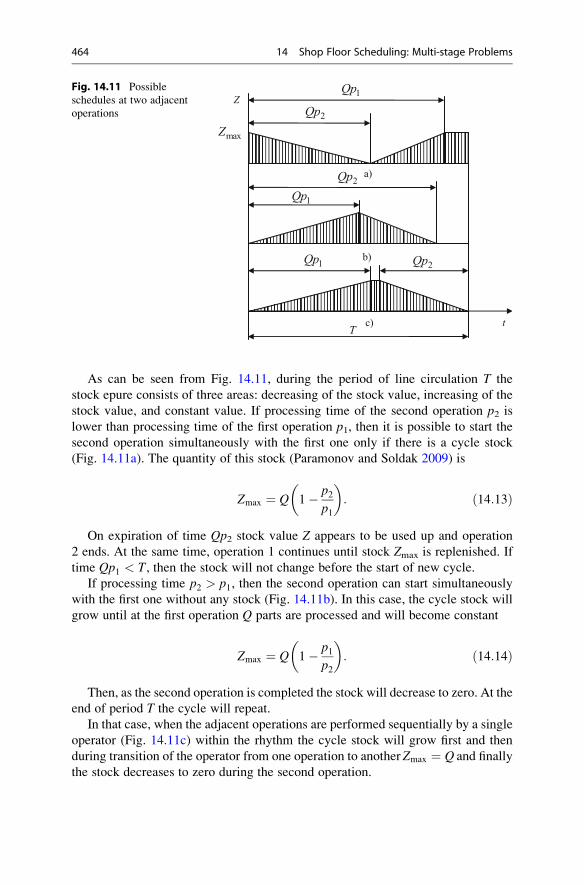
As can be seen from Fig. 14.11, during the period of line circulation T the
stock epure consists of three areas: decreasing of the stock value, increasing of the
stock value, and constant value. If processing time of the second operation p2 is
lower than processing time of the first operation p1, then it is possible to start the
second operation simultaneously with the first one only if there is a cycle stock
(Fig. 14.11a). The quantity of this stock (Paramonov and Soldak 2009) is
Zmax ¼ Q 1� p2p1
� �: ð14:13Þ
On expiration of time Qp2 stock value Z appears to be used up and operation
2 ends. At the same time, operation 1 continues until stock Zmax is replenished. If
time Qp1 < T, then the stock will not change before the start of new cycle.
If processing time p2 > p1, then the second operation can start simultaneously
with the first one without any stock (Fig. 14.11b). In this case, the cycle stock will
grow until at the first operation Q parts are processed and will become constant
Zmax ¼ Q 1� p1p2
� �: ð14:14Þ
Then, as the second operation is completed the stock will decrease to zero. At the
end of period T the cycle will repeat.
In that case, when the adjacent operations are performed sequentially by a single
operator (Fig. 14.11c) within the rhythm the cycle stock will grow first and then
during transition of the operator from one operation to another Zmax ¼ Q and finally
the stock decreases to zero during the second operation.
2Qp
T
Z1Qp
1Qp
t
2Qp
2Qp1Qp
a)
b)
c)
maxZ
Fig. 14.11 Possible
schedules at two adjacent
operations
464 14 Shop Floor Scheduling: Multi-stage Problems
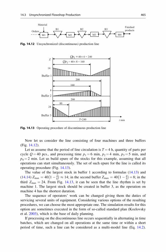
Now let us consider the line consisting of four machines and three buffers
(Fig. 14.12).
Let us assume that the period of line circulation is T¼ 4 h, quantity of parts per
cycle Q¼ 40 pcs., and processing time p1¼ 6 min, p2¼ 4 min, p3¼ 5 min, and
p4¼ 2 min. Let us build epure of the stocks for this example, assuming that all
operations can start simultaneously. The set of such epure for the line is called its
operating procedure (Fig. 14.13).
The value of the largest stock in buffer 1 according to formulas (14.13) and
(14.14) Zmax ¼ 40 1� 46
� � 14; in the second buffer Zmax ¼ 40 1� 45
� ¼ 8; in the
third Zmax ¼ 24. From Fig. 14.13, it can be seen that the line rhythm is set by
machine 1. The largest stock should be created in buffer 3, as the operation on
machine 4 has the shortest duration.
The sequence of operators’ work can be changed giving them the duties of
servicing several units of equipment. Considering various options of the resulting
procedures, we can choose the most appropriate one. The simulation results for this
option are sometimes executed in the form of so-called standard plan (Kozlovsky
et al. 2003), which is the base of daily planning.
If processing on the discontinuous line occurs sequentially in alternating in time
batches, which are changed on all operations at the same time or within a short
period of time, such a line can be considered as a multi-model line (Eq. 14.2).
Orders
Finished products
M1 M2 M4M3
B1 B2 B3
Material
Fig. 14.12 Unsynchronized (discontinuous) production line
T=240
Z1Qp = 40× 6 = 240
160
t min
2Qp = 40× 4 = 160
200
200
80
Buffer 1
Buffer 2
Buffer 3
14
8
24
Fig. 14.13 Operating procedure of discontinuous production line
14.3 Unsynchronized Flowshop Production 465
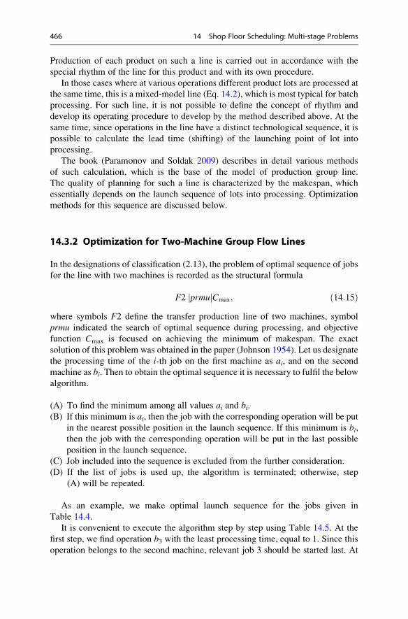
Production of each product on such a line is carried out in accordance with the
special rhythm of the line for this product and with its own procedure.
In those cases where at various operations different product lots are processed at
the same time, this is a mixed-model line (Eq. 14.2), which is most typical for batch
processing. For such line, it is not possible to define the concept of rhythm and
develop its operating procedure to develop by the method described above. At the
same time, since operations in the line have a distinct technological sequence, it is
possible to calculate the lead time (shifting) of the launching point of lot into
processing.
The book (Paramonov and Soldak 2009) describes in detail various methods
of such calculation, which is the base of the model of production group line.
The quality of planning for such a line is characterized by the makespan, which
essentially depends on the launch sequence of lots into processing. Optimization
methods for this sequence are discussed below.
14.3.2 Optimization for Two-Machine Group Flow Lines
In the designations of classification (2.13), the problem of optimal sequence of jobs
for the line with two machines is recorded as the structural formula
F2 prmuj jCmax; ð14:15Þwhere symbols F2 define the transfer production line of two machines, symbol
prmu indicated the search of optimal sequence during processing, and objective
function Cmax is focused on achieving the minimum of makespan. The exact
solution of this problem was obtained in the paper (Johnson 1954). Let us designate
the processing time of the i-th job on the first machine as ai, and on the second
machine as bi. Then to obtain the optimal sequence it is necessary to fulfil the below
algorithm.
(A) To find the minimum among all values ai and bi.(B) If this minimum is ai, then the job with the corresponding operation will be put
in the nearest possible position in the launch sequence. If this minimum is bi,then the job with the corresponding operation will be put in the last possible
position in the launch sequence.
(C) Job included into the sequence is excluded from the further consideration.
(D) If the list of jobs is used up, the algorithm is terminated; otherwise, step
(A) will be repeated.
As an example, we make optimal launch sequence for the jobs given in
Table 14.4.
It is convenient to execute the algorithm step by step using Table 14.5. At the
first step, we find operation b3 with the least processing time, equal to 1. Since this
operation belongs to the second machine, relevant job 3 should be started last. At
466 14 Shop Floor Scheduling: Multi-stage Problems

the second step, job 3 is excluded from the list, and for jobs 2 and 4, there are the
same value of minimum processing time equal to 2. Since for job 2 this minimum
refers to the first machine, then job 2 starts first. Accordingly, job 4 is placed in the
optimal sequence before already entered job 3 as the last. At the third step, we find
that job 1 should be started second in order, and finally, job 5 becomes the third in
order. This algorithm is called Johnson’s rule.
Let us use the record of the processing sequence in two entries for the first and
second machines:
machine 1 : 0 2=2ð Þ 2 1=3ð Þ 5 5=5ð Þ 10 4=4ð Þ 14 3=6ð Þ 20;machine 2 : 0=2 2=4ð Þ 6=5 1=5ð Þ 11=10 5=4ð Þ 15=14 4=2ð Þ 17=20 3=1ð Þ 21:The entry for machine 1 indicates the job start point, job number and (after slash)
processing time, and then the job end point. In the entry for machine 2, the record
structure is more complicated—here the job start point is defined as the largest
value of the machine availability time point and the readiness time point for
the operation on the second machine. It is also assumed that blocking of machine
1 by machine 2 cannot occur, i.e. the buffer capacity between these machines is
unlimited.
For example, at first machine 2 is free, but readiness of job 2 to a corresponding
operation occurs at a time equal to 2. On the contrary, for job 1 the machine
availability time point, which is 6, comes later than the time point of this job
readiness equal to 5. For job 5, its readiness comes at time point 10 and the machine
is available at point 11, etc.
In the paper (Baker and Trietsch 2009), it is proved that launching of jobs in the
sequence defined by Johnson’s rule ensures minimal idling of machine 2. Yet this
idling can become large if the processing time of an operation on the first machine
is high. In such cases, it makes sense to switch from sequential processing of each
lot to the parallel-serial processing on the time-consuming operation. Herewith the
size of a transport lot and the transfer time point of the lot to the second machine
Table 14.4 Processing
time of the jobs for the line
of two machines
Job ai bi
1 3 5
2 2 4
3 6 1
4 4 2
5 5 4
Table 14.5 Optimal
sequencingStep List of jobs min(ai, bi) Sequence
1 1, 2, 3, 4, 5 b3 {x, x, x, x, 3}
2 1, 2, 4, 5 a2, b4 {2, x, x, 4, 3}
3 1, 5 a1 {2, 1, x, 4, 3}
4 5 b5 {2, 1, 5, 4, 3}
14.3 Unsynchronized Flowshop Production 467
should be determined. The corresponding detailed analysis is presented in the book
(Paramonov and Soldak 2009).
For discontinuous production lines consisting of machines in the amount
greater than two, the problem of optimal launch is considerably complicated. To
solve it, a number of different heuristic algorithms were suggested among which
two algorithms are the most common. They are discussed below.
14.3.3 Campbell, Dudek, and Smith Algorithm
Let us consider a discontinuous production line consisting of four machines, where
it is necessary to perform five different jobs in sequence. Operating time standards
pij for them are given in Table 14.6.
Campbell, Dudek, and Smith (CDS) algorithm (Campbell et al. 1970) allows for
using Johnson’s rule for the sequence of several so-called pseudoproblems. At the
first step, it is suggested to confine oneself to considering only the first and last
machines in the line. At that, it is obvious from the previous Sect. 14.3.2 that for this
example ai ¼ pi1 and bi ¼ pi4. For illustrative purpose, these values in Table 14.6
coincide with the values in Table 14.4 and that is why Johnson’s rule at the first step
will give sequence {2, 1, 5, 4, 3}.
Let us calculate the overall duration of processing for this sequence on all four
machines:
machine1 : 0 2=2ð Þ 2 1=3ð Þ 5 5=5ð Þ 10 4=4ð Þ 14 3=6ð Þ 20;machine2 : 0=2 2=6ð Þ 8=5 1=4ð Þ 12=10 5=2ð Þ 14=14 4=3ð Þ 17=20 3=1ð Þ 21;machine3 : 0=8 2=3ð Þ 10=12 1=2ð Þ 14=14 5=3ð Þ 17=17 4=5ð Þ 22=21 3=5ð Þ 27;machine4 : 0=10 2=4ð Þ 14=14 1=5ð Þ 19=17 5=4ð Þ 23=22 4=2ð Þ 25=27 3=1ð Þ 28:
At the second and next steps of the algorithm, values ai and bi are understood asvalues
aik ¼Xkj¼1
pij and bik ¼Xm
j¼m�kþ1
pij; ð14:16Þ
where k is the step number, m is the quantity of machines in the line, and the
quantity of steps is m� 1.
Table 14.6 Processing
time of jobs for a line
consisting of four machines
Job pi1 pi2 pi3 pi4X
pi1 3 4 2 5 14
2 2 6 3 4 15
3 6 1 5 1 13
4 4 3 5 2 14
5 5 2 3 4 14
468 14 Shop Floor Scheduling: Multi-stage Problems
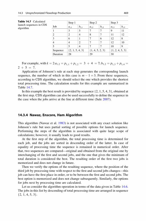
For example, with k ¼ 2 a1,2 ¼ p1,1 þ p1,2 ¼ 3 þ 4 ¼ 7; b1,2 ¼ p1,3 þ p1,4 ¼2 þ 5 ¼ 7.
Application of Johnson’s rule at each step generates the corresponding launch
sequence, the number of which in this case is m� 1 ¼ 3. From these sequences,
according to CDS algorithm, we should select the one which provides the shortest
total processing time. The calculation results for this example are summarized in
Table 14.7.
In this example the best result is provided by sequence {2, 1, 5, 4, 3}, obtained at
the first step. CDS algorithm can also be used successfully to define the sequence in
the case when the jobs arrive at the line at different time (Sule 2007).
14.3.4 Nawaz, Enscore, Ham Algorithm
This algorithm (Nawaz et al. 1983) is not associated with any exact solution like
Johnson’s rule but uses partial sorting of possible options for launch sequence.
Performing the steps of the algorithm is associated with quite large scope of
calculations; however, it usually leads to good results.
At the first step of the algorithm, the total processing time is determined for
each job, and the jobs are sorted in descending order of the latter. In case of
equality of processing time the sequence is remained in numerical order. After
that, two sequences are compared—original and obtained from the original one by
interchanging of the first and second jobs, and the one that gives the minimum of
total duration is considered the best. The resulting order of the first two jobs is
memorized and does not change in future.
Then we verify the options of the resulting sequence, where the position of the
third job by processing time with respect to the first and second jobs changes—this
job can have the first place in order, or to be between the first and second jobs. The
best option is memorized and does not change subsequently. Similarly, the options
for jobs next by processing time are calculated.
Let us consider the algorithm operation in terms of the data given in Table 14.6.
The jobs in this list by descending of total processing time are arranged in sequence
{2, 1, 4, 5, 3}.
Table 14.7 Calculated
launch sequences in CDS
algorithmJob
Step 1 Step 2 Step 3
ai,1 bi,1 ai,2 bi,2 ai,3 bi,3
1 3 5 7 7 9 11
2 2 4 8 7 11 12
3 6 1 7 6 12 8
4 4 2 7 7 12 10
5 5 4 7 7 10 9
Sequence {2, 1, 5, 4, 3} {1, 4, 5, 2, 3} {1, 2, 4, 5, 3}
Duration 28 29 30
14.3 Unsynchronized Flowshop Production 469
Let us consider two possible sequences {2, 1, 4, 5 3} and {1, 2, 4, 5, 3}, different
by execution order of the first two jobs with the highest processing time. The first of
these have the total execution duration equal to 28, and the second one—30 time
units. According Nawaz, Enscore, Ham (NEH) algorithm in this case job 2 should
be executed in all other possible sequences before job 1.
At the next step, we consider three options of launch sequence {2, 1, 4, 5, 3},
{4, 2, 1, 5, 3}, and {2, 4, 1, 5, 3} different by the position of job 4. The duration
values of these options are 28, 30, and 28 units, respectively. The second option is
clearly worse than the others, while the third option does not improve the initial
value and can be discarded as well.
Further calculation is performed for four possible options of job 5 position:
{2, 1, 4, 5, 3}, {5, 2, 1, 4, 3}, {2, 5, 1, 4, 3}, {2, 1, 5, 4, 3}. The duration values of
these options are 28, 30, 29, and 28 units, respectively. The permutation of job 5, as
we see, does not reduce the processing time compared to the first option. Finally, we
perform calculation for five possible positions of job 3: {2, 1, 4, 5, 3}, {3, 2, 1, 4, 5},
{2, 3, 1, 4, 5}, {2, 1, 3, 4, 5}, {2, 1, 4, 3, 5}, the duration of which is 28, 33, 30, 31,
and 32, respectively.
Thus, the best option is {2, 1, 4, 5, 3} with duration of 28 units. Comparing this
result with the calculation result of the optimal sequence {2, 1, 5, 4, 3}, obtained in
the previous Sect. 14.3.3, we see that the duration of the optimal options in both
algorithms is the same.
The results of applying NEH algorithm over the past 20 years, as indicated, for
example, in the paper (Kalczynski and Kamburowski 2008), show that it is highly
effective. Therefore, many researchers use this algorithm for any similar problems,
attempting to reduce the number of required iterations as well.
14.4 Job-Shop Production
In job-shop production, the sequence of operations for each job is different. At the
same time, the set of possible operations is limited by the machines at the disposal
of the production unit. The task (usually daily) of operative planning is to produce
optimal schedule of work in the department within the planned period. This period
usually covers several upcoming days, so each subsequent schedule is built based
on previously developed schedules and represents their adjustments and
amendments.
The number of possible options of the plan is extremely high in general, but it is
significantly reduced due to the factual constraints. First of all, the technology of
processing rigidly defines the possibility of equipment varying to perform
operations. Besides, for organizational and psychological reasons, as a rule, an
operation previously initiated on the machine must not be interrupted. Finally,
when scheduling it is necessary to take into account the technical condition of the
equipment, availability of tools, and qualified personnel.
Therefore, purely mathematical techniques of schedule optimization cannot lead
directly to a satisfactory result, but the schedules obtained this way can often serve
470 14 Shop Floor Scheduling: Multi-stage Problems

as a basis for making specific scheduling decisions. The method described below is
widespread and can be considered as the base in development of planning systems.
14.4.1 Shifting Bottleneck Algorithm
Let us consider the problem of execution of n jobs, each of which as going through
the technological process can come one time to mmachines or fewer machines. Let
us assume that the exact due date of each job is not stipulated and the objective
function is to minimize makespan Cmax.
In the designations of classification (2.13), the stated problem of optimal
sequence of job execution is written as a structural formula
J precj jCmax; ð14:17Þwhere symbol J means job-shop production and symbol prec means presence of
constraints of precedence during processing.
The Shifting Bottleneck Algorithm (Adams et al. 1988) is used in case of some
additional constraints of the stated problem, listed below.
(A) All jobs are available at the beginning of the scheduling.
(B) Each work cannot be performed simultaneously on several machines.
(C) The duration of each operation for each job is known.
(D) Setup and transportation time is included in the job execution time.
(E) All jobs are of equal importance.
(F) All machines are available at the beginning of work.
(G) In the department, there is only one machine of each type, and it is ready
for use.
There are several different options to use this algorithm. In this book, as in most
recent studies, we will adhere to the methods described in the book (Baker and
Trietsch 2009). For definiteness, we assume that there are three machines on which
four jobs are executed. Above in Sect. 7.5 for a similar example, it was shown that
the sequence of jobs execution is reasonable to display as a graph (Fig. 14.14).
2
31
41
2
1
3
0
0
0
0
S
2,3
1,3
2,2
3,2 3,3
E
2,1
1,1
3,1
4,2 4,32
2
Fig. 14.14 Graph of
processing four parts on three
machines
14.4 Job-Shop Production 471
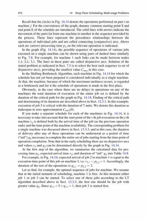
Recall that the circles in Fig. 14.14 denote the operations performed on part i onmachine j. For the convenience of the graph, dummy common starting point S and
end point E of the schedule are introduced. The solid lines with arrows indicate the
movement of the parts lot from one machine to another in the sequence provided by
the process. These lines represent the precedence relationships between the
operations of individual jobs and are called connecting (conjunctive) arcs. Above
each arc (arrow) processing time pij on the relevant operation is indicated.
In the graph (Fig. 14.14), the possible sequence of operations of various jobs
executed on a single machine can be shown using pairs of dashed lines similarly
to Fig. 7.8. For example, for machine 1 such links can be made between nodes
1,1; 2,1; 3,1. The lines in these pairs are called disjunctive arcs. Solution of the
stated problem as indicated in Sect. 7.5 is to select the best such sequence (a set of
disjunctive arcs), providing the smallest value Cmax in this case.
In the Shifting Bottleneck Algorithm, each machine in Fig. 14.14 for which the
schedule has not yet been prepared is considered individually as a single machine.
At that, the machine, because of which the maximum tardiness occurs, is regarded
as a bottleneck and for it the schedule of operations is made in the first place.
Obviously, in the case where there are no delays in operations on any of the
machines the total duration of execution of the entire job set is defined by the
duration of the critical path for the graph in Fig. 14.14. Finding of the critical path
and determining of its duration are described above in Sect. 12.3.1. In this example,
execution of job 3 is critical with the duration of 7 units. We denote this duration as
makespan in zero approximation Cmax(0).
If you make a separate schedule for each of the machines in Fig. 14.14, it is
necessary to take into account that the start point of the i-th job execution on the j-thmachine rij is defined both by the arrival time of the job (as the previous operation
ends) and the time point of the machine availability. The corresponding problem for
a single machine was discussed above in Sect. 13.3.3, and in this case, the duration
of delivery after any of these operations can be understood as a period of time
(“tail”) qij necessary to complete the entire set of jobs starting from the time point of
operation completion. Note that in the early scheduling there are no disjunctive arcs
and values rij and qij can be determined directly by the graph in Fig. 14.14.
At the first step of the algorithm, we summarize the calculated data for pro-
cessing time pij, expected arrival time rij, and duration of “tail” qij into Table 14.8.
For example, in Fig. 14.14, expected arrival of job 2 to machine 1 is equal to the
execution time point of this job on machine 3, i.e. r2,1 ¼ p2,3¼ 1. Accordingly, the
duration of the rest of the operations is q2,1 ¼ p2,2 ¼ 2.
Let us find, for example, the optimal sequence of jobs for machine. We assume
that at the initial moment of scheduling, machine 1 is free. At this moment either
job 1 or job 3 can be started. To select one of these jobs according to the LT
algorithm described above in Sect. 13.3.3, the first one should be the job with
greater value qij. Since q3,1¼ 5> q1,1¼ 1, then job 3 is started first.
472 14 Shop Floor Scheduling: Multi-stage Problems
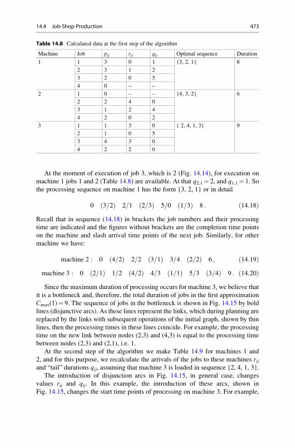
At the moment of execution of job 3, which is 2 (Fig. 14.14), for execution on
machine 1 jobs 1 and 2 (Table 14.8) are available. At that q2,1¼ 2, and q1,1¼ 1. So
the processing sequence on machine 1 has the form {3, 2, 1} or in detail
0 3=2ð Þ 2=1 2=3ð Þ 5=0 1=3ð Þ 8 : ð14:18ÞRecall that in sequence (14.18) in brackets the job numbers and their processing
time are indicated and the figures without brackets are the completion time points
on the machine and slash arrival time points of the next job. Similarly, for other
machine we have:
machine 2 : 0 4=2ð Þ 2=2 3=1ð Þ 3=4 2=2ð Þ 6 ; ð14:19Þmachine 3 : 0 2=1ð Þ 1=2 4=2ð Þ 4=3 1=1ð Þ 5=3 3=4ð Þ 9 : ð14:20ÞSince the maximum duration of processing occurs for machine 3, we believe that
it is a bottleneck and, therefore, the total duration of jobs in the first approximation
Cmax(1)¼ 9. The sequence of jobs in the bottleneck is shown in Fig. 14.15 by bold
lines (disjunctive arcs). As these lines represent the links, which during planning are
replaced by the links with subsequent operations of the initial graph, shown by thin
lines, then the processing times in these lines coincide. For example, the processing
time on the new link between nodes (2,3) and (4,3) is equal to the processing time
between nodes (2,3) and (2,1), i.e. 1.
At the second step of the algorithm we make Table 14.9 for machines 1 and
2, and for this purpose, we recalculate the arrivals of the jobs to these machines rijand “tail” durations qij, assuming that machine 3 is loaded in sequence {2, 4, 1, 3}.
The introduction of disjunction arcs in Fig. 14.15, in general case, changes
values rij and qij. In this example, the introduction of these arcs, shown in
Fig. 14.15, changes the start time points of processing on machine 3. For example,
Table 14.8 Calculated data at the first step of the algorithm
Machine Job pij rij qij Optimal sequence Duration
1 1 3 0 1 {3, 2, 1} 8
2 3 1 2
3 2 0 5
4 0 – –
2 1 0 – – {4, 3, 2} 6
2 2 4 0
3 1 2 4
4 2 0 2
3 1 1 3 0 { 2, 4, 1, 3} 9
2 1 0 5
3 4 3 0
4 2 2 0
14.4 Job-Shop Production 473
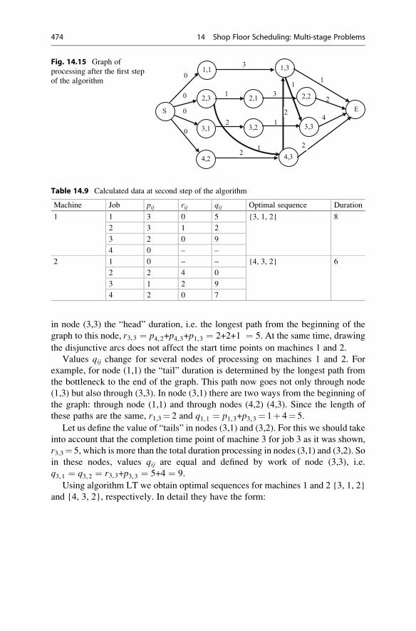
in node (3,3) the “head” duration, i.e. the longest path from the beginning of the
graph to this node, r3,3 ¼ p4,2+p4,3+p1,3 ¼ 2+2+1 ¼ 5. At the same time, drawing
the disjunctive arcs does not affect the start time points on machines 1 and 2.
Values qij change for several nodes of processing on machines 1 and 2. For
example, for node (1,1) the “tail” duration is determined by the longest path from
the bottleneck to the end of the graph. This path now goes not only through node
(1,3) but also through (3,3). In node (3,1) there are two ways from the beginning of
the graph: through node (1,1) and through nodes (4,2) (4,3). Since the length of
these paths are the same, r1,3¼ 2 and q1,1 ¼ p1,3+p3,3 ¼ 1þ 4¼ 5.
Let us define the value of “tails” in nodes (3,1) and (3,2). For this we should take
into account that the completion time point of machine 3 for job 3 as it was shown,
r3,3¼ 5, which is more than the total duration processing in nodes (3,1) and (3,2). So
in these nodes, values qij are equal and defined by work of node (3,3), i.e.
q3,1 ¼ q3,2 ¼ r3,3+p3,3 ¼ 5+4 ¼ 9.
Using algorithm LT we obtain optimal sequences for machines 1 and 2 {3, 1, 2}
and {4, 3, 2}, respectively. In detail they have the form:
1
2
31
41
2
1
3
0
0
0
0
S
2,3
1,3
2,2
3,2 3,3
E
2,1
1,1
3,1
4,2 4,32
2
2
1
Fig. 14.15 Graph of
processing after the first step
of the algorithm
Table 14.9 Calculated data at second step of the algorithm
Machine Job pij rij qij Optimal sequence Duration
1 1 3 0 5 {3, 1, 2} 8
2 3 1 2
3 2 0 9
4 0 – –
2 1 0 – – {4, 3, 2} 6
2 2 4 0
3 1 2 9
4 2 0 7
474 14 Shop Floor Scheduling: Multi-stage Problems
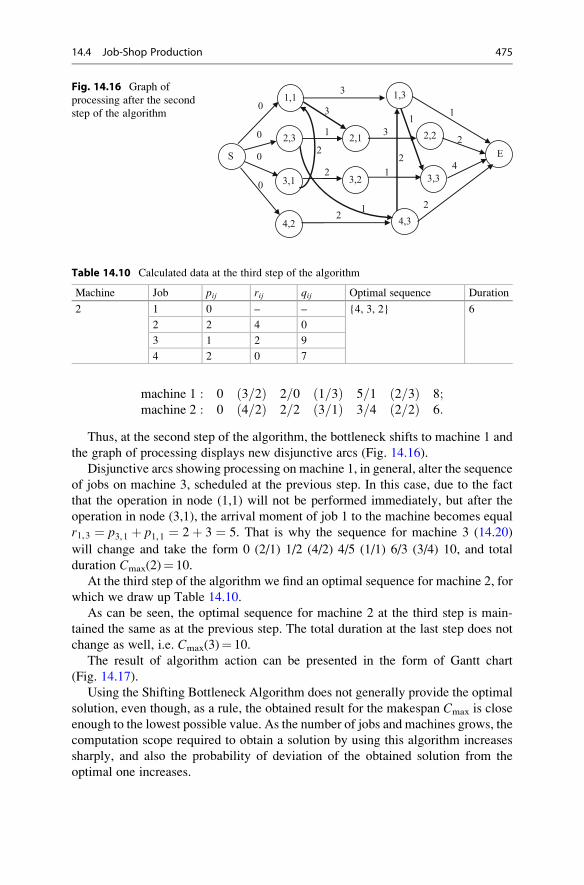
machine 1 : 0 3=2ð Þ 2=0 1=3ð Þ 5=1 2=3ð Þ 8;machine 2 : 0 4=2ð Þ 2=2 3=1ð Þ 3=4 2=2ð Þ 6:
Thus, at the second step of the algorithm, the bottleneck shifts to machine 1 and
the graph of processing displays new disjunctive arcs (Fig. 14.16).
Disjunctive arcs showing processing on machine 1, in general, alter the sequence
of jobs on machine 3, scheduled at the previous step. In this case, due to the fact
that the operation in node (1,1) will not be performed immediately, but after the
operation in node (3,1), the arrival moment of job 1 to the machine becomes equal
r1,3 ¼ p3,1 þ p1,1 ¼ 2þ 3 ¼ 5. That is why the sequence for machine 3 (14.20)
will change and take the form 0 (2/1) 1/2 (4/2) 4/5 (1/1) 6/3 (3/4) 10, and total
duration Cmax(2)¼ 10.
At the third step of the algorithm we find an optimal sequence for machine 2, for
which we draw up Table 14.10.
As can be seen, the optimal sequence for machine 2 at the third step is main-
tained the same as at the previous step. The total duration at the last step does not
change as well, i.e. Cmax(3)¼ 10.
The result of algorithm action can be presented in the form of Gantt chart
(Fig. 14.17).
Using the Shifting Bottleneck Algorithm does not generally provide the optimal
solution, even though, as a rule, the obtained result for the makespan Cmax is close
enough to the lowest possible value. As the number of jobs and machines grows, the
computation scope required to obtain a solution by using this algorithm increases
sharply, and also the probability of deviation of the obtained solution from the
optimal one increases.
3
1
2
31
41
2
1
3
0
0
0
0
S
2,3
1,3
2,2
3,2 3,3
E
2,1
1,1
3,1
4,2 4,32
2
2
1
2
Fig. 14.16 Graph of
processing after the second
step of the algorithm
Table 14.10 Calculated data at the third step of the algorithm
Machine Job pij rij qij Optimal sequence Duration
2 1 0 – – {4, 3, 2} 6
2 2 4 0
3 1 2 9
4 2 0 7
14.4 Job-Shop Production 475
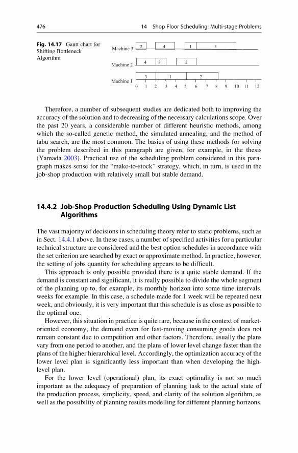
Therefore, a number of subsequent studies are dedicated both to improving the
accuracy of the solution and to decreasing of the necessary calculations scope. Over
the past 20 years, a considerable number of different heuristic methods, among
which the so-called genetic method, the simulated annealing, and the method of
tabu search, are the most common. The basics of using these methods for solving
the problem described in this paragraph are given, for example, in the thesis
(Yamada 2003). Practical use of the scheduling problem considered in this para-
graph makes sense for the “make-to-stock” strategy, which, in turn, is used in the
job-shop production with relatively small but stable demand.
14.4.2 Job-Shop Production Scheduling Using Dynamic ListAlgorithms
The vast majority of decisions in scheduling theory refer to static problems, such as
in Sect. 14.4.1 above. In these cases, a number of specified activities for a particular
technical structure are considered and the best option schedules in accordance with
the set criterion are searched by exact or approximate method. In practice, however,
the setting of jobs quantity for scheduling appears to be difficult.
This approach is only possible provided there is a quite stable demand. If the
demand is constant and significant, it is really possible to divide the whole segment
of the planning up to, for example, its monthly horizon into some time intervals,
weeks for example. In this case, a schedule made for 1 week will be repeated next
week, and obviously, it is very important that this schedule is as close as possible to
the optimal one.
However, this situation in practice is quite rare, because in the context of market-
oriented economy, the demand even for fast-moving consuming goods does not
remain constant due to competition and other factors. Therefore, usually the plans
vary from one period to another, and the plans of lower level change faster than the
plans of the higher hierarchical level. Accordingly, the optimization accuracy of the
lower level plan is significantly less important than when developing the high-
level plan.
For the lower level (operational) plan, its exact optimality is not so much
important as the adequacy of preparation of planning task to the actual state of
the production process, simplicity, speed, and clarity of the solution algorithm, as
well as the possibility of planning results modelling for different planning horizons.
Machine 3
Machine 1
Machine 2
10 2 3 4 5 6 7 8 9 10 11 12
3 1 2
234
2 4 1 3Fig. 14.17 Gantt chart for
Shifting Bottleneck
Algorithm
476 14 Shop Floor Scheduling: Multi-stage Problems
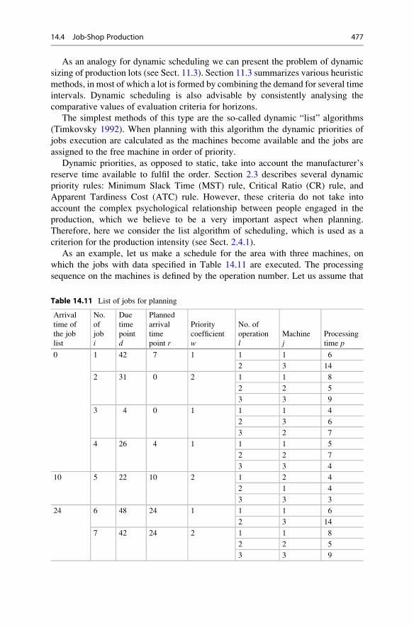
As an analogy for dynamic scheduling we can present the problem of dynamic
sizing of production lots (see Sect. 11.3). Section 11.3 summarizes various heuristic
methods, in most of which a lot is formed by combining the demand for several time
intervals. Dynamic scheduling is also advisable by consistently analysing the
comparative values of evaluation criteria for horizons.
The simplest methods of this type are the so-called dynamic “list” algorithms
(Timkovsky 1992). When planning with this algorithm the dynamic priorities of
jobs execution are calculated as the machines become available and the jobs are
assigned to the free machine in order of priority.
Dynamic priorities, as opposed to static, take into account the manufacturer’s
reserve time available to fulfil the order. Section 2.3 describes several dynamic
priority rules: Minimum Slack Time (MST) rule, Critical Ratio (CR) rule, and
Apparent Tardiness Cost (ATC) rule. However, these criteria do not take into
account the complex psychological relationship between people engaged in the
production, which we believe to be a very important aspect when planning.
Therefore, here we consider the list algorithm of scheduling, which is used as a
criterion for the production intensity (see Sect. 2.4.1).
As an example, let us make a schedule for the area with three machines, on
which the jobs with data specified in Table 14.11 are executed. The processing
sequence on the machines is defined by the operation number. Let us assume that
Table 14.11 List of jobs for planning
Arrival
time of
the job
list
No.
of
job
i
Due
time
point
d
Planned
arrival
time
point r
Priority
coefficient
w
No. of
operation
lMachine
jProcessing
time p
0 1 42 7 1 1 1 6
2 3 14
2 31 0 2 1 1 8
2 2 5
3 3 9
3 4 0 1 1 1 4
2 3 6
3 2 7
4 26 4 1 1 1 5
2 2 7
3 3 4
10 5 22 10 2 1 2 4
2 1 4
3 3 3
24 6 48 24 1 1 1 6
2 3 14
7 42 24 2 1 1 8
2 2 5
3 3 9
14.4 Job-Shop Production 477
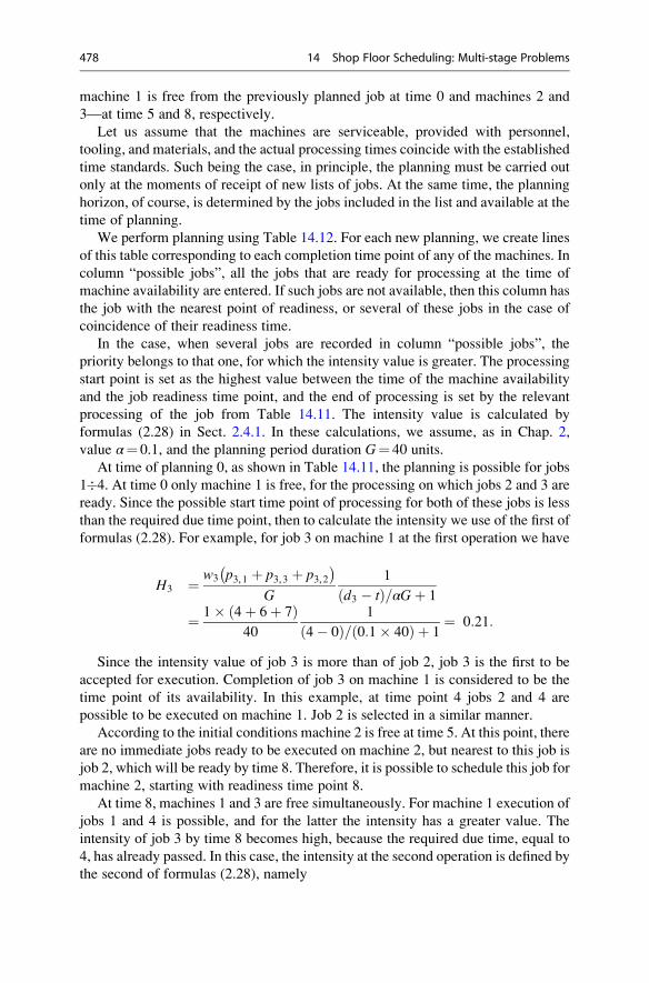
machine 1 is free from the previously planned job at time 0 and machines 2 and
3—at time 5 and 8, respectively.
Let us assume that the machines are serviceable, provided with personnel,
tooling, and materials, and the actual processing times coincide with the established
time standards. Such being the case, in principle, the planning must be carried out
only at the moments of receipt of new lists of jobs. At the same time, the planning
horizon, of course, is determined by the jobs included in the list and available at the
time of planning.
We perform planning using Table 14.12. For each new planning, we create lines
of this table corresponding to each completion time point of any of the machines. In
column “possible jobs”, all the jobs that are ready for processing at the time of
machine availability are entered. If such jobs are not available, then this column has
the job with the nearest point of readiness, or several of these jobs in the case of
coincidence of their readiness time.
In the case, when several jobs are recorded in column “possible jobs”, the
priority belongs to that one, for which the intensity value is greater. The processing
start point is set as the highest value between the time of the machine availability
and the job readiness time point, and the end of processing is set by the relevant
processing of the job from Table 14.11. The intensity value is calculated by
formulas (2.28) in Sect. 2.4.1. In these calculations, we assume, as in Chap. 2,
value α¼ 0.1, and the planning period duration G¼ 40 units.
At time of planning 0, as shown in Table 14.11, the planning is possible for jobs
1�4. At time 0 only machine 1 is free, for the processing on which jobs 2 and 3 are
ready. Since the possible start time point of processing for both of these jobs is less
than the required due time point, then to calculate the intensity we use of the first of
formulas (2.28). For example, for job 3 on machine 1 at the first operation we have
H3 ¼ w3 p3,1 þ p3,3 þ p3,2�
G
1
d3 � tð Þ=αGþ 1
¼ 1� 4þ 6þ 7ð Þ40
1
4� 0ð Þ= 0:1� 40ð Þ þ 1¼ 0:21:
Since the intensity value of job 3 is more than of job 2, job 3 is the first to be
accepted for execution. Completion of job 3 on machine 1 is considered to be the
time point of its availability. In this example, at time point 4 jobs 2 and 4 are
possible to be executed on machine 1. Job 2 is selected in a similar manner.
According to the initial conditions machine 2 is free at time 5. At this point, there
are no immediate jobs ready to be executed on machine 2, but nearest to this job is
job 2, which will be ready by time 8. Therefore, it is possible to schedule this job for
machine 2, starting with readiness time point 8.
At time 8, machines 1 and 3 are free simultaneously. For machine 1 execution of
jobs 1 and 4 is possible, and for the latter the intensity has a greater value. The
intensity of job 3 by time 8 becomes high, because the required due time, equal to
4, has already passed. In this case, the intensity at the second operation is defined by
the second of formulas (2.28), namely
478 14 Shop Floor Scheduling: Multi-stage Problems
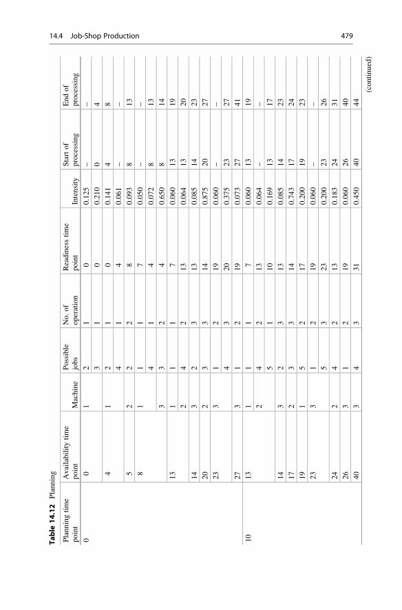
Table
14.12
Planning
Planningtime
point
Availabilitytime
point
Machine
Possible
jobs
No.of
operation
Readinesstime
point
Intensity
Startof
processing
Endof
processing
00
12
10
0.125
––
31
00.210
04
41
21
00.141
48
41
40.061
––
52
22
80.093
813
81
11
70.050
––
41
40.072
813
33
24
0.650
814
13
11
17
0.060
13
19
24
213
0.064
13
20
14
32
313
0.085
14
23
20
23
314
0.875
20
27
23
31
219
0.060
––
43
20
0.375
23
27
27
31
219
0.073
27
41
10
13
11
17
0.060
13
19
24
213
0.064
––
51
10
0.169
13
17
14
32
313
0.085
14
23
17
23
314
0.743
17
24
19
15
217
0.200
19
23
23
31
219
0.060
––
53
23
0.200
23
26
24
24
213
0.183
24
31
26
31
219
0.060
26
40
40
34
331
0.450
40
44
(continued)
14.4 Job-Shop Production 479
Table
14.12
(continued)
Planningtime
point
Availabilitytime
point
Machine
Possible
jobs
No.of
operation
Readinesstime
point
Intensity
Startof
processing
Endof
processing
24
23
16
124
0.068
––
71
24
0.191
24
32
24
24
213
0.183
24
31
26
31
219
0.072
26
40
31
27
232
0.186
32
37
32
16
124
0.100
32
38
40
34
328
0.450
40
44
62
38
0.116
––
73
37
0.300
––
–
44
36
238
0.175
––
37
337
0.675
44
53
53
36
238
0.780
53
67
480 14 Shop Floor Scheduling: Multi-stage Problems
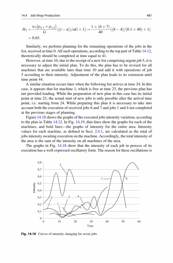
H3 ¼w3 p3,3 þ p3,2�
Gt� dið Þ=αGþ 1ð Þ ¼ 1� 6þ 7ð Þ
408� 4ð Þ= 0:1� 40ð Þ þ 1ð Þ
¼ 0:65:
Similarly, we perform planning for the remaining operations of the jobs in the
list, received at time 0. All such operations, according to the top part of Table 14.12,
theoretically should be completed at time equal to 41.
However, at time 10, due to the receipt of a new list comprising urgent job 5, it is
necessary to adjust the initial plan. To do this, the plan has to be revised for all
machines that are available later than time 10 and add it with operations of job
5 according to their intensity. Adjustment of the plan leads to its extension until
time point 44.
A similar situation occurs later when the following list arrives at time 24. In this
case, it appears that for machine 1, which is free at time 23, the previous plan has
not provided loading. While the preparation of new plan in this case has its initial
point at time 23, the actual start of new jobs is only possible after the arrival time
point, i.e. starting from 24. While preparing this plan it is necessary to take into
account both the execution of received jobs 6 and 7 and jobs 1 and 4 not completed
at the previous stages of planning.
Figure 14.18 shows the graphs of the executed jobs intensity variation, according
to the plan in Table 14.12. In Fig. 14.19, thin lines show the graphs for each of the
machines, and bold lines—the graphs of intensity for the entire area. Intensity
values for each machine, as defined in Sect. 2.4.1, are calculated as the total of
jobs intensity awaiting execution on the machine. Accordingly, the total intensity of
the area is the sum of the intensity on all machines of the area.
The graphs in Fig. 14.18 show that the intensity of each job in process of its
execution has a well expressed oscillatory form. The reason for these oscillations is
0
0,1
0,2
0,3
0,4
0,5
0,6
0,7
0,8
0 10 20 30 40 50 60
Intensity
Time
3
5 4
1
7 6
2
Fig. 14.18 Curves of intensity changing for seven jobs
14.4 Job-Shop Production 481
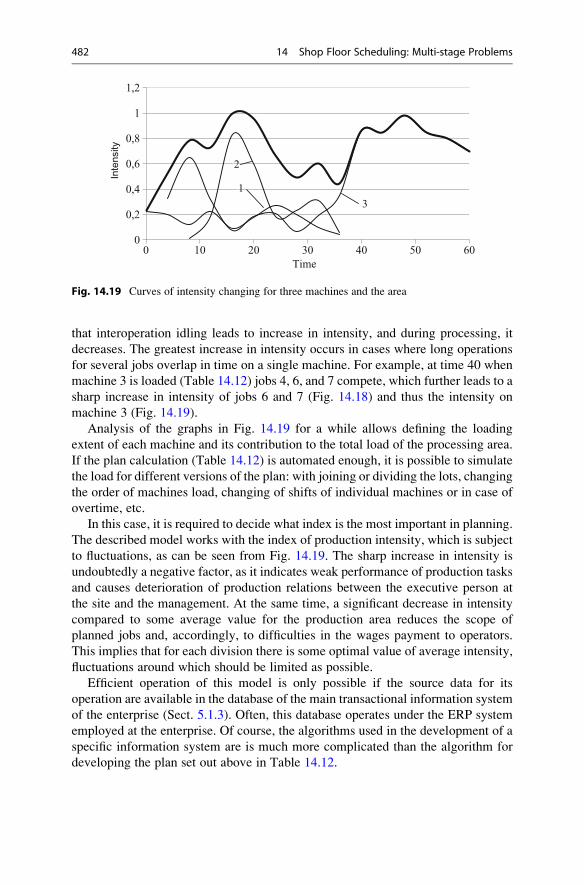
that interoperation idling leads to increase in intensity, and during processing, it
decreases. The greatest increase in intensity occurs in cases where long operations
for several jobs overlap in time on a single machine. For example, at time 40 when
machine 3 is loaded (Table 14.12) jobs 4, 6, and 7 compete, which further leads to a
sharp increase in intensity of jobs 6 and 7 (Fig. 14.18) and thus the intensity on
machine 3 (Fig. 14.19).
Analysis of the graphs in Fig. 14.19 for a while allows defining the loading
extent of each machine and its contribution to the total load of the processing area.
If the plan calculation (Table 14.12) is automated enough, it is possible to simulate
the load for different versions of the plan: with joining or dividing the lots, changing
the order of machines load, changing of shifts of individual machines or in case of
overtime, etc.
In this case, it is required to decide what index is the most important in planning.
The described model works with the index of production intensity, which is subject
to fluctuations, as can be seen from Fig. 14.19. The sharp increase in intensity is
undoubtedly a negative factor, as it indicates weak performance of production tasks
and causes deterioration of production relations between the executive person at
the site and the management. At the same time, a significant decrease in intensity
compared to some average value for the production area reduces the scope of
planned jobs and, accordingly, to difficulties in the wages payment to operators.
This implies that for each division there is some optimal value of average intensity,
fluctuations around which should be limited as possible.
Efficient operation of this model is only possible if the source data for its
operation are available in the database of the main transactional information system
of the enterprise (Sect. 5.1.3). Often, this database operates under the ERP system
employed at the enterprise. Of course, the algorithms used in the development of a
specific information system are is much more complicated than the algorithm for
developing the plan set out above in Table 14.12.
0
0,2
0,4
0,6
0,8
1
1,2
0 10 20 30 40 50 60
Intensity
Time
2
1
3
Fig. 14.19 Curves of intensity changing for three machines and the area
482 14 Shop Floor Scheduling: Multi-stage Problems
References
Adams, J., Balas, E., & Zawack, D. (1988). The shifting bottleneck algorithm for job-shop
scheduling. Management Science, 34, 391–401.Baker, K. R., & Trietsch, D. (2009). Principles of sequencing and scheduling. New York: Wiley.
Bartholdi, J. J., & Eisenstein, D. D. (1996). A production line that balances itself. OperationsResearch, 44, 21–34.
Becker, C., & Scholl, A. (2006). A survey on problems and methods in generalized assembly line
balancing. European Journal of Operational Research, 168, 694–715.Bluemenfeld, D. E., & Li, J. (2005). An analytical formula for throughput of a production line with
identical stations and random failures. Mathematical Problems in Engineering, 3, 293–308.Burbidge, J. L. (1991). Production flow analysis for planning group technology. Journal of
Operations Management, 10, 5–27.Burbidge, J. L. (1997). Production flow analysis for planning group technology. Oxford: Oxford
University Press.
Campbell, H. G., Dudek, R. A., & Smith, M. I. (1970). A heuristic algorithm for n-job, m-machine
sequencing problem. Management Science, 16, 630–637.Johnson, S. M. (1954). Optimal two-and three-stage production schedules with setup times
included. Naval Research Logistic Quarterly, 1, 61–68.Kalczynski, P. J., & Kamburowski, J. (2008). An improved NEH heuristic to minimize makespan
in permutation flow shops. Computers and Operations Research, 35, 3001–3008.Kozlovsky, V. A., Kazantsev, A. K., Kobzev, V. V., Kuzin, B. I., Makarov, V. M., & Smirnov,
A. V. (2003). Production management. Moscow: Infra-M (in Russian).
Li, J., & Meerkov, S. M. (2009). Production systems engineering. New York: Springer.
Lobanskaya, L. P., & Sergina, M. T. (1969). Revising the definition of rhythmical production at oil
refineries. Chemistry and Technology of Fuels and Oils, 9, 39–42 (in Russian).
McCormick, S. T., Pinedo, M. L., Shenker, S., & Wolf, B. (1989). Sequencing in an assembly line
with blocking to minimize cycle time. Operations Research, 37, 925–936.Monden, Y. (1983). Toyota production system. Norcross, GA: Industrial Engineering and Man-
agement Press.
Nawaz, M. E., Enscore, E., & Ham, J. (1983). A heuristic algorithm for m-machine n-job flow-
shop sequencing problem. Omega, International Journal of Management Science, 11, 91–95.Paramonov, F. I., & Soldak, Y. M. (2009). Theoretical foundations of production management,
BINOM. Moscow: Laboratoriya znaniy (in Russian).
Pinedo, M. L. (2005). Planning and scheduling in manufacturing and services. Berlin: Springer.Quadt, D. (2004). Lot-sizing and scheduling for flexible flow lines. Berlin: Springer.Ribas, I., Leisten, R., & Frami~nan, J. M. (2010). Review and classification of hybrid flow shop
scheduling problems from a production system and a solutions procedure perspective.
Computers and Operations Research, 37, 1439–1454.Ruiz, R., & Vazquez-Rodrıguez, J. A. (2010). The hybrid flow shop scheduling problem.
European Journal of Operational Research, 205, 1–18.Sule, D. R. (2007). Production planning and industrial scheduling. London: Taylor & Francis
Group.
Timkovsky, V. G. (1992). Discrete mathematics in the world of machines and tools. Moscow:
Nauka (in Russian).
Vladzievsky, A. R. (1950). Theory of internal stocks and their influence on automatic lines
performance, Part 1. Machines and Tools, 21, 4–7 (in Russian).
Vladzievsky, A. R. (1951). Theory of internal stocks and their influence on automatic lines
performance, Part 2. Machines and Tools, 22, 16–17 (in Russian).
Yamada, T. (2003). Studies on metaheuristics for jobshop and flowshop scheduling problems.
Kyoto University, Kyoto. www.kecl.ntt.co.jp/. . ./YamadaThesis.pdf
References 483

Multi-criteria Scheduling 15
15.1 Just-in-Time Production Scheduling
For Just-in-Time (JiT) production, the schedule of starting different jobs should
provide a regular supply of components to assembly exactly according to needs
arisen. However, since the supply of components is possible only in lots, the sizes
of which are often determined by the cost of setup and transportation, the dates
necessary for lots to arrive to assembly are not always known. The values of these
dates are determined by establishing a certain compromise between the possibility
of delay and undesired long storing.
As a rule, in the studies on optimal JiT schedules the criteria are used based on
the values of tardiness of deliveries Ti and waiting for release Ei. Two such
algorithms for relatively simple cases are given below.
15.1.1 Starting Group of Jobs with Fixed Sequence
Let us consider the problem of scheduling for a single machine, which must pro-
cess a group of jobs (product lots), for each of which desired delivery date di isestablished. It is also assumed that the sequence of these jobs is known and the
objective functions are both minimization of total tardiness T and early production
E of the entire group of jobs. The relevant classification formula of the problem has
the form
1��di, seq�� f T;Eð Þ; ð15:1Þ
where parameter seq is the symbol of the predefined sequence. In the simplest case,
the objective functions has the form
# Springer International Publishing Switzerland 2016
Y. Mauergauz, Advanced Planning and Scheduling in Manufacturing and SupplyChains, DOI 10.1007/978-3-319-27523-9_15
485
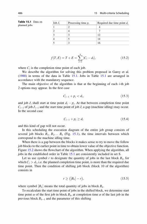
f T;Eð Þ ¼ T þ E ¼Xni¼1
Ci � dij j; ð15:2Þ
where Ci is the completion time point of each job.
We describe the algorithm for solving this problem proposed in Garey et al.
(1988) in terms of the data in Table 15.1. Jobs in Table 15.1 are arranged in
accordance with the mandatory sequence.
The main objective of the algorithm is that at the beginning of each i-th job
2 options may appear. In the first case
Ci�1 þ pi < di; ð15:3Þand job Ji shall start at time point di � pi. At that between completion time point
Ci�1 of job Ji�1 and the start time point of job Ji a gap (machine idling) may occur.
In the second case
Ci�1 þ pi � di ð15:4Þand this kind of gap will not occur.
In this scheduling the execution diagram of the entire job group consists of
several job blocks B1, B2. . . Bk (Fig. 15.1), the time intervals between which
correspond to the machine idling time.
When there is a gap between the blocks it makes sense to try to move the follow
job blocks to the earlier point in time to obtain lower value of the objective function.
Figure 15.2 shows the flowchart of the algorithm. When applying the algorithm, all
jobs in the established order in Table 15.1 are consistently included in set S.
Let us use symbol r to designate the quantity of jobs in the last block Bk, for
whichCi > di, i.e. the planned completion time point, is more than the required due
time point. Then the condition of shifting job block (block 10 of the algorithm)
consists in
r � ��Bk
��� r�
; ð15:5Þ
where symbol��Bk
�� means the total quantity of jobs in block Bk.
To recalculate the start time point of jobs in the shifted block, we determine start
time point ω of the first job in block Bk, at completion time π of the last job in the
previous block Bk�1 and the parameter of this shifting
Table 15.1 Data on
planned jobsJob Ji Processing time pi Required due time point di
1 2 4
2 4 7
3 3 12
4 5 14
5 3 16
486 15 Multi-criteria Scheduling
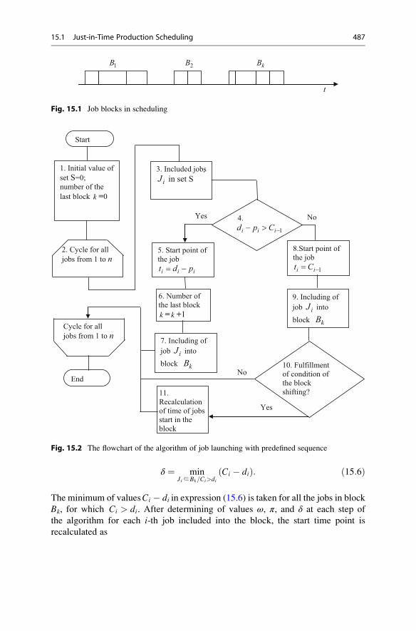
δ ¼ minJi ∈Bk=Ci>di
Ci � dið Þ: ð15:6Þ
The minimum of valuesCi � di in expression (15.6) is taken for all the jobs in blockBk, for which Ci > di. After determining of values ω, π, and δ at each step of
the algorithm for each i-th job included into the block, the start time point is
recalculated as
1B 2B kB
t
Fig. 15.1 Job blocks in scheduling
Cycle for all
jobs from 1 to n
Start
1. Initial value of
set S=0;
number of the
last block k =0
10. Fulfillment of condition of the block shifting?
4.
1i i id p C −− >
End
11. Recalculation of time of jobs start in the block
5. Start point of the job
i i it d p= −
3. Included jobs
iJ in set S
Yes No
8.Start point of the job
1i it C −=
6. Number of the last block
k = k +1
7. Including of
job iJ into
block kB
9. Including of
job iJ into
block kB
2. Cycle for all
jobs from 1 to n
Yes
No
Fig. 15.2 The flowchart of the algorithm of job launching with predefined sequence
15.1 Just-in-Time Production Scheduling 487
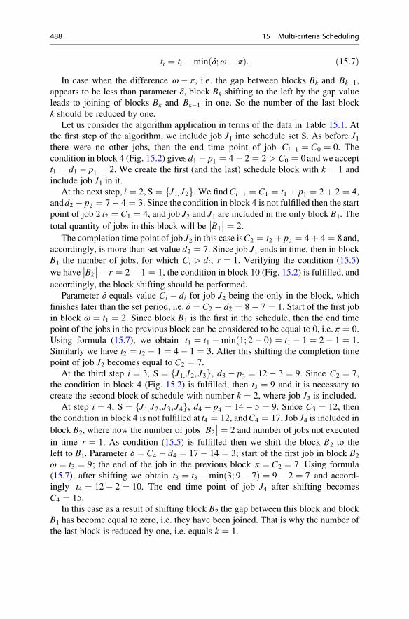
ti ¼ ti �min δ;ω� πð Þ: ð15:7ÞIn case when the difference ω� π, i.e. the gap between blocks Bk and Bk�1,
appears to be less than parameter δ, block Bk shifting to the left by the gap value
leads to joining of blocks Bk and Bk�1 in one. So the number of the last block
k should be reduced by one.
Let us consider the algorithm application in terms of the data in Table 15.1. At
the first step of the algorithm, we include job J1 into schedule set S. As before J1there were no other jobs, then the end time point of job Ci�1 ¼ C0 ¼ 0. The
condition in block 4 (Fig. 15.2) gives d1 � p1 ¼ 4� 2 ¼ 2 > C0 ¼ 0 and we accept
t1 ¼ d1 � p1 ¼ 2. We create the first (and the last) schedule block with k ¼ 1 and
include job J1 in it.
At the next step, i ¼ 2, S ¼ J1, J2f g. We find Ci�1 ¼ C1 ¼ t1 þ p1 ¼ 2þ 2 ¼ 4,
andd2 � p2 ¼ 7� 4 ¼ 3. Since the condition in block 4 is not fulfilled then the start
point of job 2 t2 ¼ C1 ¼ 4, and job J2 and J1 are included in the only block B1. The
total quantity of jobs in this block will be��B1
�� ¼ 2.
The completion time point of job J2 in this case isC2 ¼ t2 þ p2 ¼ 4þ 4 ¼ 8and,
accordingly, is more than set value d2 ¼ 7. Since job J1 ends in time, then in block
B1 the number of jobs, for which Ci > di, r ¼ 1. Verifying the condition (15.5)
we have��Bk
��� r ¼ 2� 1 ¼ 1, the condition in block 10 (Fig. 15.2) is fulfilled, and
accordingly, the block shifting should be performed.
Parameter δ equals value Ci � di for job J2 being the only in the block, which
finishes later than the set period, i.e. δ ¼ C2 � d2 ¼ 8� 7 ¼ 1. Start of the first job
in block ω ¼ t1 ¼ 2. Since block B1 is the first in the schedule, then the end time
point of the jobs in the previous block can be considered to be equal to 0, i.e. π ¼ 0.
Using formula (15.7), we obtain t1 ¼ t1 �min 1; 2� 0ð Þ ¼ t1 � 1 ¼ 2� 1 ¼ 1.
Similarly we have t2 ¼ t2 � 1 ¼ 4� 1 ¼ 3. After this shifting the completion time
point of job J2 becomes equal to C2 ¼ 7.
At the third step i ¼ 3, S ¼ J1, J2, J3f g, d3 � p3 ¼ 12� 3 ¼ 9. Since C2 ¼ 7,
the condition in block 4 (Fig. 15.2) is fulfilled, then t3 ¼ 9 and it is necessary to
create the second block of schedule with number k ¼ 2, where job J3 is included.At step i ¼ 4, S ¼ J1, J2, J3, J4f g, d4 � p4 ¼ 14� 5 ¼ 9. Since C3 ¼ 12, then
the condition in block 4 is not fulfilled at t4 ¼ 12, andC4 ¼ 17. Job J4 is included in
block B2, where now the number of jobs��B2
�� ¼ 2 and number of jobs not executed
in time r ¼ 1. As condition (15.5) is fulfilled then we shift the block B2 to the
left to B1. Parameter δ ¼ C4 � d4 ¼ 17� 14 ¼ 3; start of the first job in block B2
ω ¼ t3 ¼ 9; the end of the job in the previous block π ¼ C2 ¼ 7. Using formula
(15.7), after shifting we obtain t3 ¼ t3 �min 3; 9� 7ð Þ ¼ 9� 2 ¼ 7 and accord-
ingly t4 ¼ 12� 2 ¼ 10. The end time point of job J4 after shifting becomes
C4 ¼ 15.
In this case as a result of shifting block B2 the gap between this block and block
B1 has become equal to zero, i.e. they have been joined. That is why the number of
the last block is reduced by one, i.e. equals k ¼ 1.
488 15 Multi-criteria Scheduling
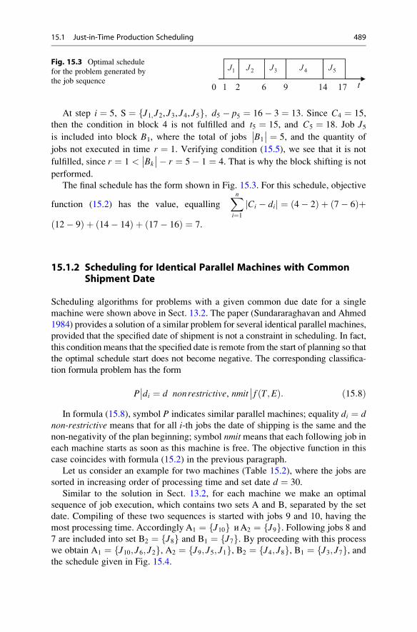
At step i ¼ 5, S ¼ J1, J2, J3, J4, J5f g; d5 � p5 ¼ 16� 3 ¼ 13. Since C4 ¼ 15,
then the condition in block 4 is not fulfilled and t5 ¼ 15, and C5 ¼ 18. Job J5is included into block B1, where the total of jobs
��B1
�� ¼ 5, and the quantity of
jobs not executed in time r ¼ 1. Verifying condition (15.5), we see that it is not
fulfilled, since r ¼ 1 <��Bk
��� r ¼ 5� 1 ¼ 4. That is why the block shifting is not
performed.
The final schedule has the form shown in Fig. 15.3. For this schedule, objective
function (15.2) has the value, equallingXni¼1
Ci � dij j ¼ 4� 2ð Þ þ 7� 6ð Þþ12� 9ð Þ þ 14� 14ð Þ þ 17� 16ð Þ ¼ 7.
15.1.2 Scheduling for Identical Parallel Machines with CommonShipment Date
Scheduling algorithms for problems with a given common due date for a single
machine were shown above in Sect. 13.2. The paper (Sundararaghavan and Ahmed
1984) provides a solution of a similar problem for several identical parallel machines,
provided that the specified date of shipment is not a constraint in scheduling. In fact,
this condition means that the specified date is remote from the start of planning so that
the optimal schedule start does not become negative. The corresponding classifica-
tion formula problem has the form
P��di ¼ d nonrestrictive, nmit
�� f T;Eð Þ: ð15:8ÞIn formula (15.8), symbol P indicates similar parallel machines; equality di ¼ d
non-restrictive means that for all i-th jobs the date of shipping is the same and the
non-negativity of the plan beginning; symbol nmitmeans that each following job in
each machine starts as soon as this machine is free. The objective function in this
case coincides with formula (15.2) in the previous paragraph.
Let us consider an example for two machines (Table 15.2), where the jobs are
sorted in increasing order of processing time and set date d ¼ 30.
Similar to the solution in Sect. 13.2, for each machine we make an optimal
sequence of job execution, which contains two sets A and B, separated by the set
date. Compiling of these two sequences is started with jobs 9 and 10, having the
most processing time. Accordingly A1 ¼ J10f g иA2 ¼ J9f g. Following jobs 8 and7 are included into set B2 ¼ J8f g and B1 ¼ J7f g. By proceeding with this process
we obtain A1 ¼ J10; J6; J2f g, A2 ¼ J9; J5; J1f g, B2 ¼ J4; J8f g, B1 ¼ J3; J7f g, andthe schedule given in Fig. 15.4.
t0 1 2 6 9 14 17
2J 3J1J 4J 5JFig. 15.3 Optimal schedule
for the problem generated by
the job sequence
15.1 Just-in-Time Production Scheduling 489
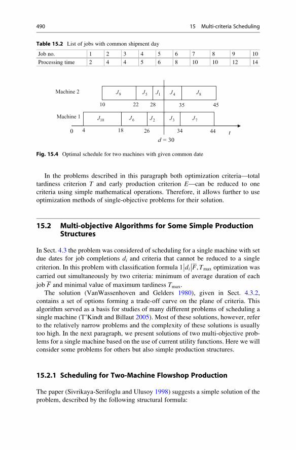
In the problems described in this paragraph both optimization criteria—total
tardiness criterion T and early production criterion E—can be reduced to one
criteria using simple mathematical operations. Therefore, it allows further to use
optimization methods of single-objective problems for their solution.
15.2 Multi-objective Algorithms for Some Simple ProductionStructures
In Sect. 4.3 the problem was considered of scheduling for a single machine with set
due dates for job completions di and criteria that cannot be reduced to a single
criterion. In this problem with classification formula 1��di��F,Tmax optimization was
carried out simultaneously by two criteria: minimum of average duration of each
job F and minimal value of maximum tardiness Tmax.
The solution (VanWassenhoven and Gelders 1980), given in Sect. 4.3.2,
contains a set of options forming a trade-off curve on the plane of criteria. This
algorithm served as a basis for studies of many different problems of scheduling a
single machine (T’Kindt and Billaut 2005). Most of these solutions, however, refer
to the relatively narrow problems and the complexity of these solutions is usually
too high. In the next paragraph, we present solutions of two multi-objective prob-
lems for a single machine based on the use of current utility functions. Here we will
consider some problems for others but also simple production structures.
15.2.1 Scheduling for Two-Machine Flowshop Production
The paper (Sivrikaya-Serifoglu and Ulusoy 1998) suggests a simple solution of the
problem, described by the following structural formula:
Table 15.2 List of jobs with common shipment day
Job no. 1 2 3 4 5 6 7 8 9 10
Processing time 2 4 4 5 6 8 10 10 12 14
t0 4
10
18 26 34 44
6J 2J10J 3J 7J
5J 1J9J 4J 8JMachine 2
Machine 1
d = 30
35 452822
Fig. 15.4 Optimal schedule for two machines with given common date
490 15 Multi-criteria Scheduling
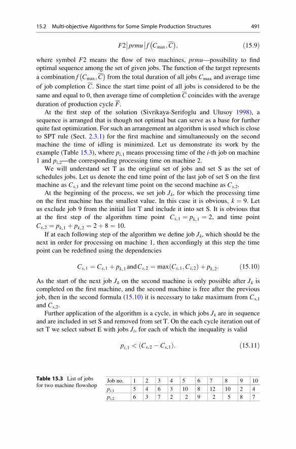
F2��prmu �� f Cmax;C
� ; ð15:9Þ
where symbol F2 means the flow of two machines, prmu—possibility to find
optimal sequence among the set of given jobs. The function of the target represents
a combination f Cmax;C�
from the total duration of all jobs Cmax and average time
of job completion C. Since the start time point of all jobs is considered to be the
same and equal to 0, then average time of completion C coincides with the average
duration of production cycle F.At the first step of the solution (Sivrikaya-Serifoglu and Ulusoy 1998), a
sequence is arranged that is though not optimal but can serve as a base for further
quite fast optimization. For such an arrangement an algorithm is used which is close
to SPT rule (Sect. 2.3.1) for the first machine and simultaneously on the second
machine the time of idling is minimized. Let us demonstrate its work by the
example (Table 15.3), where pi,1 means processing time of the i-th job on machine
1 and pi,2—the corresponding processing time on machine 2.
We will understand set T as the original set of jobs and set S as the set of
schedules jobs. Let us denote the end time point of the last job of set S on the first
machine as Cs,1 and the relevant time point on the second machine as Cs,2.
At the beginning of the process, we set job Jk, for which the processing time
on the first machine has the smallest value. In this case it is obvious, k ¼ 9. Let
us exclude job 9 from the initial list T and include it into set S. It is obvious that
at the first step of the algorithm time point Cs, 1 ¼ pk, 1 ¼ 2, and time point
Cs, 2 ¼ pk, 1 þ pk, 2 ¼ 2þ 8 ¼ 10.
If at each following step of the algorithm we define job Jk, which should be the
next in order for processing on machine 1, then accordingly at this step the time
point can be redefined using the dependencies
Cs, 1 ¼ Cs, 1 þ pk, 1 andCs, 2 ¼ max Cs, 1;Cs, 2ð Þ þ pk, 2: ð15:10ÞAs the start of the next job Jk on the second machine is only possible after Jk iscompleted on the first machine, and the second machine is free after the previous
job, then in the second formula (15.10) it is necessary to take maximum from Cs,1
and Cs,2.
Further application of the algorithm is a cycle, in which jobs Jk are in sequence
and are included in set S and removed from set T. On the each cycle iteration out of
set T we select subset E with jobs Ji, for each of which the inequality is valid
pi, 1 < Cs, 2 � Cs, 1ð Þ: ð15:11Þ
Table 15.3 List of jobs
for two machine flowshopJob no. 1 2 3 4 5 6 7 8 9 10
pi,1 5 4 6 3 10 8 12 10 2 4
pi,2 6 3 7 2 2 9 2 5 8 7
15.2 Multi-objective Algorithms for Some Simple Production Structures 491

If subset E appears to be empty, then as the next job Jk, we select that one, forwhich
pk, 1 ¼ minJi ∈T
pi, 1�
; ð15:12Þ
otherwise, the number of the following job k is defined as
pk, 1 ¼ minJi ∈E
pi, 1�
: ð15:13Þ
In that case, when it appears that in formula (15.12) or (15.13) there are several
jobs with the same values pi,1, the job with the least value pi,2 is accepted as Jk. Afterdefining Jk, this job is transferred from set T to set S; values Cs,1 and Cs,2 are
recalculated by formulas (15.10). When set T becomes empty the cycle stops.
In this example at the first cycle iteration Cs, 2 � Cs, 1ð Þ ¼ 10� 2 ¼ 8 and all the
jobs, for which pi, 1 < 8 are included into set E, i.e. E ¼ J1; J2; J3; J4; J10f g.According to formula (15.13) the next in the planned sequence job J4 appears, forwhich we have the least p4,1 ¼ 3. By recalculating values Cs,1 and Cs,2 by formulas
(15.10), we haveCs, 1 ¼ 2þ 3 ¼ 5,Cs, 2 ¼ max 5, 10ð Þ þ 2 ¼ 12, and S ¼ J9; J4f g.By continuing the operation of the cycle, at the second iteration we have
Cs, 2 � Cs, 1ð Þ ¼ 7 and set E ¼ J1; J2; J3; J10f g. Since p2,1 ¼ p10,1 ¼ 4, so as the
next job we accept job J2 with valuep2,2 ¼ 3 < p10,2 ¼ 7. The planned list after this
iteration S ¼ J9; J4; J2f g. We recalculate Cs, 1 ¼ 9; Cs, 2 ¼ 15.
At the third iteration Cs, 2 � Cs, 1ð Þ ¼ 6; set E ¼ J1; J10f g. Accordingly k ¼ 10
and S ¼ J9; J4; J2; J10f g. We recalculate Cs, 1 ¼ 13; Cs, 2 ¼ 22.
At the following iteration, Cs, 2 � Cs, 1ð Þ ¼ 9 ; set E ¼ J1; J3; J6f g ; k ¼ 1 ;
S ¼ J9; J4; J2; J10; J1f g; Cs, 1 ¼ 18; Cs, 2 ¼ 28.
Then Cs, 2 � Cs, 1ð Þ ¼ 8 ; E ¼ J3f g ; S ¼ J9; J4; J2; J10; J1; J3f g ; Cs, 1 ¼ 24 ;
Cs, 2 ¼ 35.
Onward Cs, 2 � Cs, 1ð Þ ¼ 9; E ¼ J6f g; S ¼ J9; J4; J2; J10; J1; J3; J6f g; Cs, 1 ¼ 32;
Cs, 2 ¼ 44.
Similarly Cs, 2 � Cs, 1ð Þ ¼ 10; set E is empty. According to expression (15.12)
we have two possibilities—jobs J5 and J8. Since for the first of them value pi,2is less than for the second we obtain sequence S ¼ J9; J4; J2; J10; J1; J3; J6; J5f g,Cs, 1 ¼ 42, Cs, 2 ¼ 46.
At the following iteration Cs, 2 � Cs, 1ð Þ ¼ 4, set E is empty; we add job J8 to set
S. At thatCs, 1 ¼ 52,Cs, 2 ¼ max Cs, 1;Cs, 2ð Þ þ pk, 2 ¼ max 52, 46ð Þ þ 5 ¼ 57 and in
this case machine 2 will be idling.
The similar idling will be also before job J7. Finally, we have the sequence
S ¼ J9; J4; J2; J10; J1; J3; J6; J5; J8; J7f g, for which Gantt charts are valid, shown inFig. 15.5.
From Fig. 15.5 it immediately follows thatCmax ¼ 66. The average duration of a
production cycle is defined as a sum of all end points of jobs on the second machine,
referred to the total of jobs and equal to F ¼ 33:5.
492 15 Multi-criteria Scheduling
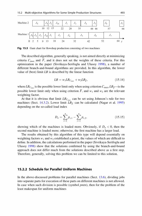
The described algorithm, generally speaking, is not aimed directly at minimizing
criteria Cmax and F, and it does not set the weights of these criteria. For this
optimization in the paper (Sivrikaya-Serifoglu and Ulusoy 1998), a number of
different branch-and-bound algorithms are provided. In this algorithm, the lower
value of (best) limit LB is described by the linear function
LB ¼ w1LBCmaxþ w2LBF; ð15:14Þ
whereLBCmaxis the possible lower limit only when using criterion Cmax,LBF—is the
possible lower limit only when using criterion F, and w1 and w2 are the relevant
weighting factor.
At that it is obvious that limit LBCmaxcan be set using Johnson’s rule for two
machines (Sect. 14.3.2). Lower limit LBF can be calculated (Nagar et al. 1995)
depending on the so-called load index
Da ¼Xni¼1
pi, 1 �Xni¼1
pi, 2; ð15:15Þ
showing which of the machines is loaded more. Obviously, if Da < 0, then the
second machine is loaded more; otherwise, the first machine has a larger load.
The results obtained by this algorithm of this type will depend essentially on
weighting factors w1 and w2 established a priori, the values of which are difficult to
define. In addition, the calculations performed in the paper (Sivrikaya-Serifoglu and
Ulusoy 1998) show that the solutions confirmed by using the branch-and-bound
approach does not differ much from the solutions described above as a first step.
Therefore, generally, solving this problem we can be limited to this solution.
15.2.2 Schedule for Parallel Uniform Machines
In the above-discussed problems for parallel machines (Sect. 13.6), dividing jobs
into separate parts for execution of these parts on different machines is not allowed.
In case when such division is possible (symbol pmtn), then for the problem of the
least makespan for uniform machines
15
Machine 1
t
12
0 2
10
13 24 42 52
2J9J 10J 5J
4J 2J9J 10J 6JMachine 2
35 442822
4J
5 9
1J
18
1J 3J
6J
32
5J
46
8J
8J
57
7J
7J
64
66
3J
Fig. 15.5 Gant chart for flowshop production consisting of two machines
15.2 Multi-objective Algorithms for Some Simple Production Structures 493
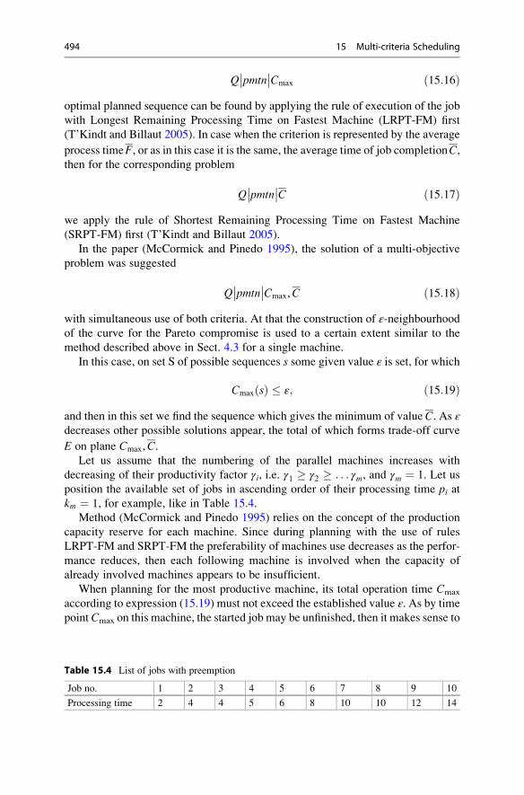
Q��pmtn��Cmax ð15:16Þ
optimal planned sequence can be found by applying the rule of execution of the job
with Longest Remaining Processing Time on Fastest Machine (LRPT-FM) first
(T’Kindt and Billaut 2005). In case when the criterion is represented by the average
process timeF, or as in this case it is the same, the average time of job completionC,then for the corresponding problem
Q��pmtn��C ð15:17Þ
we apply the rule of Shortest Remaining Processing Time on Fastest Machine
(SRPT-FM) first (T’Kindt and Billaut 2005).
In the paper (McCormick and Pinedo 1995), the solution of a multi-objective
problem was suggested
Q��pmtn��Cmax,C ð15:18Þ
with simultaneous use of both criteria. At that the construction of ε-neighbourhoodof the curve for the Pareto compromise is used to a certain extent similar to the
method described above in Sect. 4.3 for a single machine.
In this case, on set S of possible sequences s some given value ε is set, for which
Cmax sð Þ � ε; ð15:19Þ
and then in this set we find the sequence which gives the minimum of valueC. As εdecreases other possible solutions appear, the total of which forms trade-off curve
E on plane Cmax,C.Let us assume that the numbering of the parallel machines increases with
decreasing of their productivity factor γi, i.e. γ1 � γ2 � . . . γm, and γm ¼ 1. Let us
position the available set of jobs in ascending order of their processing time pi atkm ¼ 1, for example, like in Table 15.4.
Method (McCormick and Pinedo 1995) relies on the concept of the production
capacity reserve for each machine. Since during planning with the use of rules
LRPT-FM and SRPT-FM the preferability of machines use decreases as the perfor-
mance reduces, then each following machine is involved when the capacity of
already involved machines appears to be insufficient.
When planning for the most productive machine, its total operation time Cmax
according to expression (15.19) must not exceed the established value ε. As by time
point Cmax on this machine, the started job may be unfinished, then it makes sense to
Table 15.4 List of jobs with preemption
Job no. 1 2 3 4 5 6 7 8 9 10
Processing time 2 4 4 5 6 8 10 10 12 14
494 15 Multi-criteria Scheduling
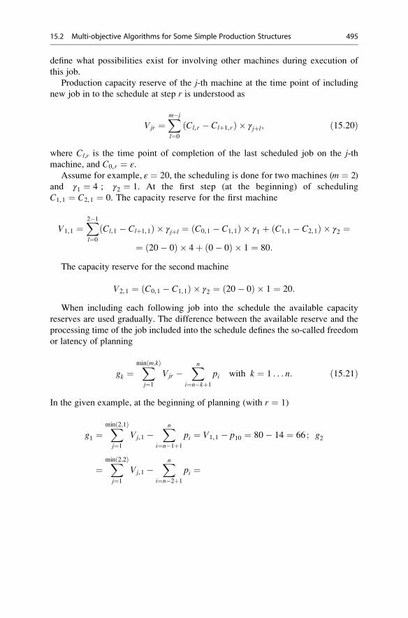
define what possibilities exist for involving other machines during execution of
this job.
Production capacity reserve of the j-th machine at the time point of including
new job in to the schedule at step r is understood as
Vjr ¼Xm�j
l¼0
Cl, r � Clþ1, rð Þ � γjþl; ð15:20Þ
where Cl,r is the time point of completion of the last scheduled job on the j-thmachine, and C0, r ¼ ε.
Assume for example, ε ¼ 20, the scheduling is done for two machines (m ¼ 2)
and γ1 ¼ 4 ; γ2 ¼ 1. At the first step (at the beginning) of scheduling
C1,1 ¼ C2,1 ¼ 0. The capacity reserve for the first machine
V1,1 ¼X2�1
l¼0
Cl, 1 � Clþ1,1ð Þ � γjþl ¼ C0,1 � C1,1ð Þ � γ1 þ C1,1 � C2,1ð Þ � γ2 ¼¼ 20� 0ð Þ � 4þ 0� 0ð Þ � 1 ¼ 80:
The capacity reserve for the second machine
V2,1 ¼ C0,1 � C1,1ð Þ � γ2 ¼ 20� 0ð Þ � 1 ¼ 20:
When including each following job into the schedule the available capacity
reserves are used gradually. The difference between the available reserve and the
processing time of the job included into the schedule defines the so-called freedom
or latency of planning
gk ¼Xmin m;kð Þ
j¼1
Vjr �Xn
i¼n�kþ1
pi with k ¼ 1 . . . n: ð15:21Þ
In the given example, at the beginning of planning (with r ¼ 1)
g1 ¼Xmin 2;1ð Þ
j¼1
Vj, 1 �Xn
i¼n�1þ1
pi ¼ V1,1 � p10 ¼ 80� 14 ¼ 66 ; g2
¼Xmin 2;2ð Þ
j¼1
Vj, 1 �Xn
i¼n�2þ1
pi ¼
15.2 Multi-objective Algorithms for Some Simple Production Structures 495

¼ V1,1 þ V2,1 � p10 � p9 ¼ 80þ 20� 14� 12 ¼ 74; g3
¼Xmin 2;3ð Þ
j¼1
Vj, 1 �Xn
i¼n�3þ1
pi ¼
¼ V1,1 þ V2,1 � p10 � p9 � p8 ¼ 64; g4 ¼ 54; g5 ¼ 46; g6 ¼ 40 g7 ¼ 35; g8¼ 31; g9 ¼ 27
and g10 ¼ 25. The required condition of scheduling possibility is the condition
gk � 0 with r ¼ 1 forallk ¼ 1 . . . n: ð15:22ÞIn the block diagram shown in Fig. 15.6, auxiliary set of jobs T is used that is
initially equal to the original set sorted in ascending order of the processing time.
Calculation of initial values Cl,1, Vj,1, and gk is described above; if some of gk < 0,
then calculation is terminated.
At each step r of the cycle (block 4) there is a machine which is free first (block
5). After defining the minimal value gk two options are possible. If g > 0, then rule
SRPT-FM is used and the first out of jobs of set T (block 8) is included in the
schedule of machine j for the time equalling x. In the other option, rule LRPT-FM
(block 9) is used and the last job out of set T is included into the machine schedule.
Value x is defined by one of three methods. For the least productive machine
with productivity coefficient γm ¼ 1, value
x ¼ min Cj�1, r � Cj, r,piγj, g Tj j
!ð15:23Þ
where��T�� is the quantity of items in set T. In this example, initial value
��T�� ¼ 10.
If γj � γm ¼ 1, we use the formula
x ¼ min Cj�1, r � Cj, r,piγj, minl¼iþ1...
��T��‐1 gl0@ 1A; ð15:24Þ
and in other cases
x ¼ min Cj�1, r � Cj, r,piγj,
g Tj jγj � γm � 1
,
minl¼iþ1...
��T��‐1 glγj � γm
!: ð15:25Þ
If the value obtained from formulas (15.23–15.25) x < pi=γj (block 12 in
Fig. 15.6), then job Ji is performed on the j-th machine incompletely, and the
remainder should be included in the schedule of other machine at the following
iteration of the algorithm. After defining set T (block 13), it is necessary to
recalculate (block 15) values Cl,r as
496 15 Multi-criteria Scheduling
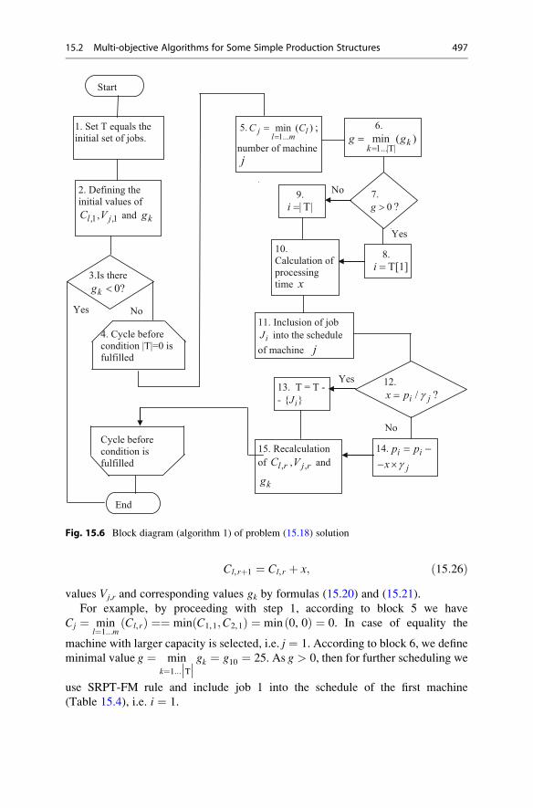
Cl, rþ1 ¼ Cl, r þ x; ð15:26Þvalues Vj,r and corresponding values gk by formulas (15.20) and (15.21).
For example, by proceeding with step 1, according to block 5 we have
Cj ¼ minl¼1...m
Cl, rð Þ ¼¼ min C1,1;C2,1ð Þ ¼ min 0, 0ð Þ ¼ 0. In case of equality the
machine with larger capacity is selected, i.e. j ¼ 1. According to block 6, we define
minimal value g ¼ mink¼1...
��T�� gk ¼ g10 ¼ 25. As g > 0, then for further scheduling we
use SRPT-FM rule and include job 1 into the schedule of the first machine
(Table 15.4), i.e. i ¼ 1.
Start
1. Set T equals the initial set of jobs.
12.
/i jx p γ= ?
7.
0g > ?
End
6.
1...|T|min ( )k
kg g
==
Yes
No
2. Defining the initial values of
,1lC , ,1jV and kg
No
8.
T[1]i =
5.1...
min ( )j ll m
C C=
= ;
number of machine
j
10. Calculation ofprocessing time x
11. Inclusion of job
iJ into the schedule
of machine j
13. T = T -
- { }iJ
14. i ip p= −
jx γ− ×15. Recalculation
of ,l rC , ,j rV and
kg
3.Is there
kg < 0?
Yes
Yes
9.
| T|i =
4. Cycle before condition |T|=0 is fulfilled
Cycle before condition is fulfilled
No
Fig. 15.6 Block diagram (algorithm 1) of problem (15.18) solution
15.2 Multi-objective Algorithms for Some Simple Production Structures 497
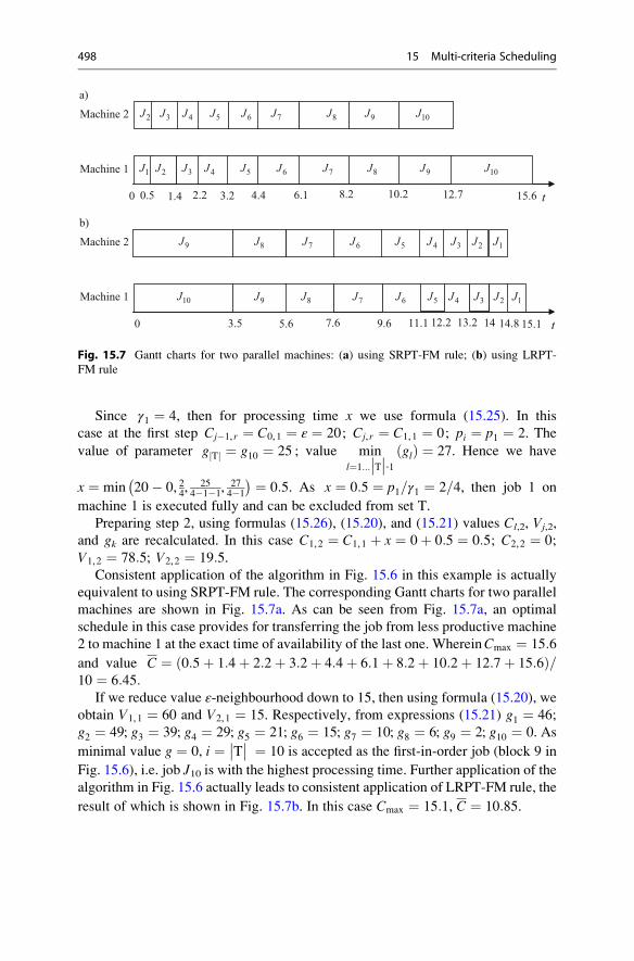
Since γ1 ¼ 4, then for processing time x we use formula (15.25). In this
case at the first step Cj�1, r ¼ C0,1 ¼ ε ¼ 20; Cj, r ¼ C1,1 ¼ 0; pi ¼ p1 ¼ 2. The
value of parameter g Tj j ¼ g10 ¼ 25 ; value minl¼1...
��T��‐1 glð Þ ¼ 27. Hence we have
x ¼ min 20� 0, 24, 254�1�1
, 274�1
� ¼ 0:5. As x ¼ 0:5 ¼ p1=γ1 ¼ 2=4, then job 1 on
machine 1 is executed fully and can be excluded from set T.
Preparing step 2, using formulas (15.26), (15.20), and (15.21) values Cl,2, Vj,2,
and gk are recalculated. In this case C1,2 ¼ C1,1 þ x ¼ 0þ 0:5 ¼ 0:5; C2,2 ¼ 0;
V1,2 ¼ 78:5; V2,2 ¼ 19:5.Consistent application of the algorithm in Fig. 15.6 in this example is actually
equivalent to using SRPT-FM rule. The corresponding Gantt charts for two parallel
machines are shown in Fig. 15.7a. As can be seen from Fig. 15.7a, an optimal
schedule in this case provides for transferring the job from less productive machine
2 to machine 1 at the exact time of availability of the last one. WhereinCmax ¼ 15:6
and value C ¼ 0:5þ 1:4þ 2:2þ 3:2þ 4:4þ 6:1þ 8:2þ 10:2þ 12:7þ 15:6ð Þ=10 ¼ 6:45:
If we reduce value ε-neighbourhood down to 15, then using formula (15.20), we
obtain V1,1 ¼ 60 and V2,1 ¼ 15. Respectively, from expressions (15.21) g1 ¼ 46;
g2 ¼ 49; g3 ¼ 39; g4 ¼ 29; g5 ¼ 21; g6 ¼ 15; g7 ¼ 10; g8 ¼ 6; g9 ¼ 2; g10 ¼ 0. As
minimal value g ¼ 0, i ¼ ��T�� ¼ 10 is accepted as the first-in-order job (block 9 in
Fig. 15.6), i.e. job J10 is with the highest processing time. Further application of the
algorithm in Fig. 15.6 actually leads to consistent application of LRPT-FM rule, the
result of which is shown in Fig. 15.7b. In this case Cmax ¼ 15:1, C ¼ 10:85.
Machine 1
t0 0.5 3.2 6.1 10.2 15.6
1J 3J 7J
4J 5J 6J 9JMachine 2
1.4 2.2
4J
4.4
7J 8J
6J
8.2
10J
8J 9J5J
2J
2J
3J
12.7
10J
Machine 1
t0 3.5 5.6 9.6 14
10J 8J
Machine 2
12.27.6
7J 6J9J
9J
11.1
5J 4J
13.2
3J
a)
b)
8J 7J 6J 5J 4J 3J 2J
14.8
1J
1J2J
15.1
Fig. 15.7 Gantt charts for two parallel machines: (a) using SRPT-FM rule; (b) using LRPT-
FM rule
498 15 Multi-criteria Scheduling
Comparing the obtained results in Fig. 15.7a, b, we see that the use of LRPT-FM
rule leads to a slight decrease in the total processing time Cmax, but significantly
increases the average processing time of a job C.The paper (McCormick and Pinedo 1995) describes a general algorithm that
allows finding a few non-dominated options of scheduling, which use partly SRPT-
FM rule and partly LRPT-FM rule. In this case, the algorithm in Fig. 15.6 is part of
a more general algorithm. The complexity of the latter, however, is that its
presentation in the scope of this book is not possible.
In practical terms, when solving the above problem it can be recommended first
to find solutions according to SRPT-FM and LRPT-FM rules using the algorithm in
Fig. 15.6. Then, if it is desirable to reduce the overall processing time Cmax, then
some jobs with greater processing time should be moved to the beginning of the
schedule drawn up by SRPT-FM rule.
15.2.3 Some Other Problems and Solving Challenges
Above in Sects. 4.3 and 15.2.2, three problems of multi-objective scheduling were
considered: for a single machine, for two successive machines, and for uniform
parallel machines. For these and similar to them industrial structures, a large
number of studies were carried out with different set of criteria and constraints.
Let us consider a few such examples, starting with the tasks for a single machine.
The paper (Lin 1983) considers the problem with classification formula
1��di��C, T; ð15:27Þ
close to the described in Sect. 4.3 problem with formula 1��di��F,Tmax. Virtually, the
difference is in the fact that in the first case the criterion of average tardiness T is
applied, while in the second case the criterion is the greatest tardiness Tmax. As for
the criteria of the average job completion timeC and the average processing timeF,then if all the jobs are available by the start time point of planning then these criteria
are equal. The use of criterion T required to apply a quite complex algorithm based
on dynamic programming method when solving the problem (Lin 1983) of finding
Pareto solution.
The need for the multi-objective approach is expressed usually not for the
problems with two temporal criteria as F,Tmax or C, T, but in the tasks, in which
one of the criteria describes the time consumption, and the second criteria defines
the cost values. The cost values for the problems of scheduling are mainly in the
costs for changeover of the machine when transferring from one job to another.
In the paper (Bourgade et al. 1995) a typical task of this kind with structural
formula is considered
1��di, sik��F c; Tmaxð Þ; ð15:28Þ
15.2 Multi-objective Algorithms for Some Simple Production Structures 499
where sikmeans availability of time consumption for changeover from job i to job k.The objective function here is some function F c; Tmaxð Þ of average setup cost c andmaximal tardiness Tmax. As this kind of function for n job it was suggested, for
example, to use the expression of the form
F c; Tmaxð Þ ¼ w1cþ w2
Xni¼1
exp max 0, Ti � T*max
� � ; ð15:29Þ
where Tmax is understood as the problem solution with formula 1��di��Tmax; w1 and
w2—some weighting factors. This problem (Bourgade et al. 1995) was solved by
branch-and-bound method.
Among the studies relating to scheduling for flowshop production, the problem
outstands
F2��prmu, di��Cmax,Tmax: ð15:30Þ
In the framework of this problem for two sequential machines with possible
permutations of jobs (prmu) and given due dates di in Daniels and Chambers
(1990), a heuristic method for finding the optimal sequence was developed,
which is close to the method of solving the problem, detailed above in Sect. 4.3.
The developed method allows by use of special ε-neighbourhood of efficient points(Sect. 4.3.1) to find Pareto solutions and construct a trade-off curve for different
schedule options. Moreover, in the paper (Daniels and Chambers 1990), it was also
proposed to extend this method for the case of any number of serial arranged
machines, i.e. for the problem
F��prmu, di��Cmax,Tmax: ð15:31Þ
For identical parallel machines, substantial results are obtained in the paper
(Mohri et al. 1999), which allowed solving the problem
P3��pmtn, di��Cmax,Lmax: ð15:32Þ
In this paper, for three machines with specified due dates di and the possibility tointerrupt jobs (pmtn), Pareto non-dominated solutions for two criteria are found—
the makespan Cmax and the greatest deviation Lmax from the specified due date.
Returning to three problems described above in Sects. 4.2 and 15.2.2, one can
notice that the complete solution including the trade-off curve construction between
the criteria was given only for the first one, which is the most simple. For the other
two tasks, due to the complexity of calculations, we had to be limited to only a
partial their solution. Such a solution consists in scheduling for individual possible
non-dominated options without constructing a complete Pareto solution.
Naturally, for the tasks described above in this paragraph, we had to develop
even more complex algorithms than those given in Sect. 15.2.2. Also, while solving
500 15 Multi-criteria Scheduling

these problems the required scope of computation may depend heavily on the
number of independent variables of planning (jobs and machines).
In some simple cases, such as in problems in Sect. 4.3 or Sect. 15.2.2, the scope
of computation is a polynomial dependence on the number of variables. However,
for so-called NP-hard problems, which are typical for the majority of planning
cases, a much stronger growth in the scope of calculations is possible.
The concept of NP-hard is a quite difficult mathematical definition and it is
usually believed that the NP-hard problems are those that have the scope of
calculation exponentially depending on the number of variables. Not only complex
problems but also simple ones can be NP-hard. For example, NP-hard problem is
the problem for the flowshop production consisting of two machines, described in
Sect. 15.2.1.
Due to the difficulty in computing of the majority of known algorithms, even
with theoretical solutions, the practical use of multi-objective scheduling is limited
to our time. In recent years, however, a large number of paper and studies are
dedicated to development of new, as a rule, heuristic methods for finding optimal
solutions. In these studies analogies to a variety of situations are used, for example,
the behaviour of living things, etc.
The reason for such rapid growth of researches in this field is apparently initiated
awareness of the fact that the optimization of operational planning in many cases
cannot be achieved with a single criterion and requires the inclusion of at least two
criteria, as it has been shown in Fig. 4.5.
A detailed overview of the major jobs in the field of multi-objective schedules
for flowshop and job shop production over the past two decades is presented, for
example, here (Parveen and Ullah 2010).
15.3 Scheduling Based on Cost and Average Orders Utility
Let us consider operational planning for a single machine in terms of serial
production and “make-to-order” strategy. According to Table 2.5 it is advantageous
here to use a schedule with two criteria—minimum costs K1 and timely order
fulfilment C1. These criteria are contradictory, since, for example, to reduce K1 it is
necessary to increase the sizes of production lots and conversely, to reduce the
delay of order fulfilment C1 the lot sizes should be reduced. Thus, problems of this
type have the so-called planning dilemma described previously in Sect. 3.2.
As shown above in Sect. 4.1.3, criterion C1 can be replaced by utility function of
order processing V and criterion K1—by cost function U (Fig. 4.5). To solve the
problem of planning with the help of these functions, it is necessary to construct the
corresponding Pareto solution (trade-off curve) and then select a positioning point
of this curve, i.e. specific solution that suits best the planner’s ideas at the time of
planning. Below there are two examples of such an approach for planning the
operation of a single machine. Using this methodology for parallel machines, job
shop production is described in Mauergauz (2013).
15.3 Scheduling Based on Cost and Average Orders Utility 501
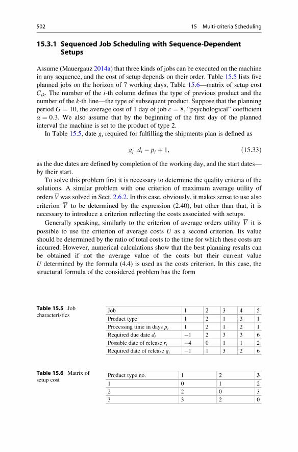
15.3.1 Sequenced Job Scheduling with Sequence-DependentSetups
Assume (Mauergauz 2014a) that three kinds of jobs can be executed on the machine
in any sequence, and the cost of setup depends on their order. Table 15.5 lists five
planned jobs on the horizon of 7 working days, Table 15.6—matrix of setup cost
Cik. The number of the i-th column defines the type of previous product and the
number of the k-th line—the type of subsequent product. Suppose that the planning
period G ¼ 10, the average cost of 1 day of job c ¼ 8, “psychological” coefficient
α ¼ 0:3. We also assume that by the beginning of the first day of the planned
interval the machine is set to the product of type 2.
In Table 15.5, date gi required for fulfilling the shipments plan is defined as
gi¼di � pi þ 1; ð15:33Þas the due dates are defined by completion of the working day, and the start dates—
by their start.
To solve this problem first it is necessary to determine the quality criteria of the
solutions. A similar problem with one criterion of maximum average utility of
ordersVwas solved in Sect. 2.6.2. In this case, obviously, it makes sense to use also
criterion V to be determined by the expression (2.40), but other than that, it is
necessary to introduce a criterion reflecting the costs associated with setups.
Generally speaking, similarly to the criterion of average orders utility V it is
possible to use the criterion of average costs �U as a second criterion. Its value
should be determined by the ratio of total costs to the time for which these costs are
incurred. However, numerical calculations show that the best planning results can
be obtained if not the average value of the costs but their current value
U determined by the formula (4.4) is used as the costs criterion. In this case, the
structural formula of the considered problem has the form
Table 15.5 Job
characteristicsJob 1 2 3 4 5
Product type 1 2 1 3 1
Processing time in days pi 1 2 1 2 1
Required due date di �1 2 3 3 6
Possible date of release ri �4 0 1 1 2
Required date of release gi �1 1 3 2 6
Table 15.6 Matrix of
setup costProduct type no. 1 2 3
1 0 1 2
2 2 0 3
3 3 2 0
502 15 Multi-criteria Scheduling
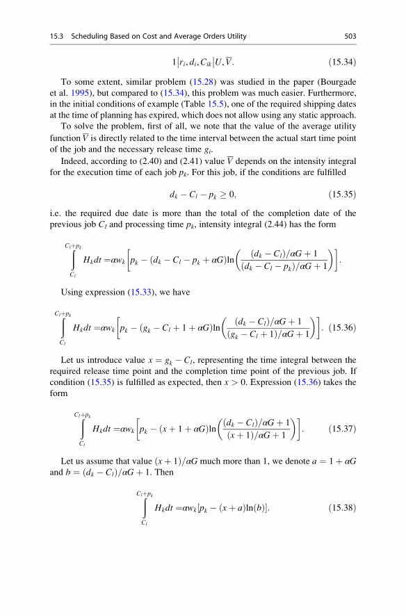
1��ri, di,Cik
��U,V: ð15:34ÞTo some extent, similar problem (15.28) was studied in the paper (Bourgade
et al. 1995), but compared to (15.34), this problem was much easier. Furthermore,
in the initial conditions of example (Table 15.5), one of the required shipping dates
at the time of planning has expired, which does not allow using any static approach.
To solve the problem, first of all, we note that the value of the average utility
function V is directly related to the time interval between the actual start time point
of the job and the necessary release time gi.
Indeed, according to (2.40) and (2.41) value V depends on the intensity integral
for the execution time of each job pk. For this job, if the conditions are fulfilled
dk � Cl � pk � 0; ð15:35Þi.e. the required due date is more than the total of the completion date of the
previous job Cl and processing time pk, intensity integral (2.44) has the form
ðClþpk
Cl
Hkdt ¼αwk pk � dk � Cl � pk þ αGð Þln dk � Clð Þ=αGþ 1
dk � Cl � pkð Þ=αGþ 1
� � �:
Using expression (15.33), we have
ðClþpk
Cl
Hkdt ¼αwk pk � gk � Cl þ 1þ αGð Þln dk � Clð Þ=αGþ 1
gk � Cl þ 1ð Þ=αGþ 1
� � �: ð15:36Þ
Let us introduce value x ¼ gk � Cl, representing the time integral between the
required release time point and the completion time point of the previous job. If
condition (15.35) is fulfilled as expected, then x > 0. Expression (15.36) takes the
form
ðClþpk
Cl
Hkdt ¼αwk pk � xþ 1þ αGð Þln dk � Clð Þ=αGþ 1
xþ 1ð Þ=αGþ 1
� � �: ð15:37Þ
Let us assume that value xþ 1ð Þ=αG much more than 1, we denote a ¼ 1þ αGand b ¼ dk � Clð Þ=αGþ 1. Then
ðClþpk
Cl
Hkdt ¼αwk pk � xþ að Þln bð Þ½ �: ð15:38Þ
15.3 Scheduling Based on Cost and Average Orders Utility 503
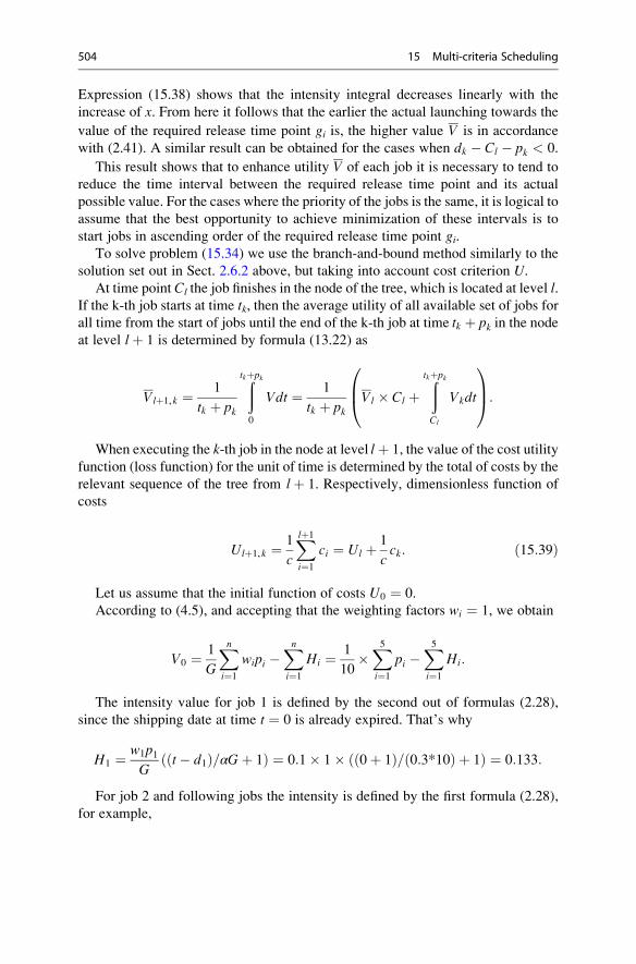
Expression (15.38) shows that the intensity integral decreases linearly with the
increase of x. From here it follows that the earlier the actual launching towards the
value of the required release time point gi is, the higher value V is in accordance
with (2.41). A similar result can be obtained for the cases when dk � Cl � pk < 0.
This result shows that to enhance utility V of each job it is necessary to tend to
reduce the time interval between the required release time point and its actual
possible value. For the cases where the priority of the jobs is the same, it is logical to
assume that the best opportunity to achieve minimization of these intervals is to
start jobs in ascending order of the required release time point gi.To solve problem (15.34) we use the branch-and-bound method similarly to the
solution set out in Sect. 2.6.2 above, but taking into account cost criterion U.At time point Cl the job finishes in the node of the tree, which is located at level l.
If the k-th job starts at time tk, then the average utility of all available set of jobs forall time from the start of jobs until the end of the k-th job at time tk þ pk in the nodeat level lþ 1 is determined by formula (13.22) as
Vlþ1,k ¼ 1
tk þ pk
ðtkþpk
0
Vdt ¼ 1
tk þ pkVl � Cl þ
ðtkþpk
Cl
Vkdt
0B@1CA:
When executing the k-th job in the node at level lþ 1, the value of the cost utility
function (loss function) for the unit of time is determined by the total of costs by the
relevant sequence of the tree from lþ 1. Respectively, dimensionless function of
costs
Ulþ1,k ¼ 1
c
Xlþ1
i¼1
ci ¼ Ul þ 1
cck: ð15:39Þ
Let us assume that the initial function of costs U0 ¼ 0.
According to (4.5), and accepting that the weighting factors wi ¼ 1, we obtain
V0 ¼ 1
G
Xni¼1
wipi �Xni¼1
Hi ¼ 1
10�X5i¼1
pi �X5i¼1
Hi:
The intensity value for job 1 is defined by the second out of formulas (2.28),
since the shipping date at time t ¼ 0 is already expired. That’s why
H1 ¼ w1p1G
t� d1ð Þ=αGþ 1ð Þ ¼ 0:1� 1� 0þ 1ð Þ= 0:3*10ð Þ þ 1ð Þ ¼ 0:133:
For job 2 and following jobs the intensity is defined by the first formula (2.28),
for example,
504 15 Multi-criteria Scheduling
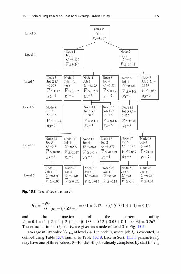
H2 ¼ w2p2G
1
d2 � tð Þ=αGþ 1¼ 0:1� 2= 2� 0ð Þ= 0:3*10ð Þ þ 1ð Þ ¼ 0:12
and the function of the current utility
V0 ¼ 0:1� 1þ 2þ 1þ 2þ 1ð Þ � 0:133þ 0:12þ 0:05þ 0:1þ 0:03ð Þ ¼ 0:267.The values of initial U0 and V0 are given as a node of level 0 in Fig. 15.8.
Average utility value Vlþ1,q at level lþ 1 in node q, where job Jk is executed, is
defined using Table 15.7, similar to Table 13.18. Like in Sect. 13.5.3 parameter aikmay have one of three values: 0—for the i-th jobs already completed by start time tk
Node 2Job 2
U = 0
V ≤ 0.143
Node 1Job 1
U =0.125
V ≤ 0.244
Node 5
Job 4 U=0.5
V ≤ 0.152
4g = 2
Node 6Job 1
U =0.125
V ≤ 0.108
1g = -1
Node 0
0U =0
0V =0.267
Level 1
Level 0
Level 2
Level 3
Level 4
Node 8Job 4
U =0.25
V ≤ 0.033
4g = 2
Node 7
Job 3 U =
0.125
V ≤ 0.086
3g = 3
Node 4Job 3
U =0.125
V ≤ 0.207
3g = 3
Node 3
Job 2 U=0.375
V ≤ 0.17
2g = 1
Node 10
Job 5 U=0.125
V ≤ 0.145
4g = 6
Node 9Job 3
U =0.5
V ≤ 0.129
3g = 3
Node 11
Job 2 U=0.375
V ≤ 0.115
2g = 1
Node 12
Job 3 U =
0.125
V ≤ 0.082
3g = 3
Node 13Job 5
U =0.5
V ≤ 0.086
5g = 6
Node 14Job 4
U =0.875
V ≤ 0.027
4g = 2
Node 15Job 4
U =0.625
V ≤ 0.019
4g = 2
Node 18Job 4
U =0.5
V ≤ 0.00
4g = 2
Node 17Job 5
U =0.125
V ≤ 0.049
5g = 6
Node 23Job 4
U =0.5
V ≤ -0.1
Node 24Job 5
U =0.75
V ≤ 0.00
Node 19Job 4
U =0.875
V ≤ -0.07
Node 21Job 5
U =0.875
V ≤ 0.015
Node 20Job 5
U =1.125
V ≤ 0.022
Level 5
Node 16Job 2
U =0.375
V ≤ -0.019
2g = 1
Node 22Job 4
U =0.625
V ≤ -0.13
Fig. 15.8 Tree of decisions search
15.3 Scheduling Based on Cost and Average Orders Utility 505
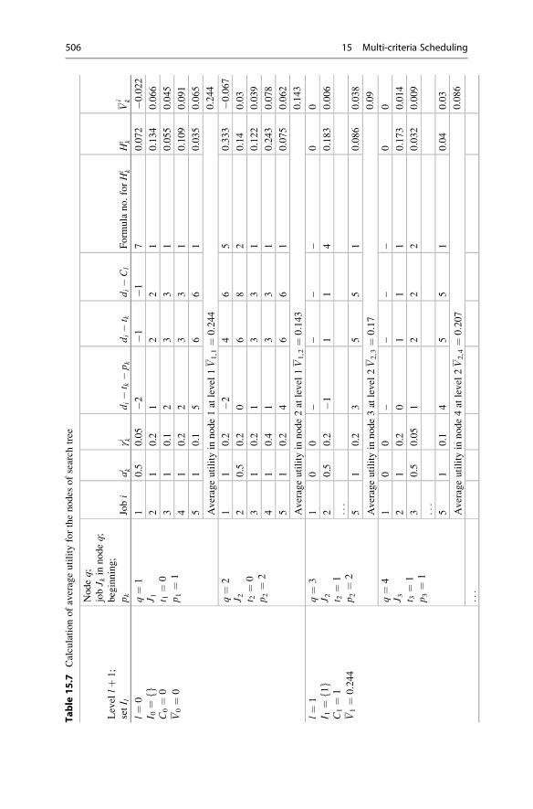
Table
15.7
Calculationofaverageutility
forthenodes
ofsearch
tree
Level
lþ1;
setI l
Nodeq;
jobJ k
innodeq;
beginning;
pk
Jobi
ai k
γi kdi�t k�pk
di�t k
di�Cl
Form
ula
no.forH
i kH
i kV
i k
l¼
0
I 0¼
fgC0¼
0
V0¼
0
q¼
1
J 1 t 1¼
0
p1¼
1
10.5
0.05
�2�1
�17
0.072
�0.022
21
0.2
12
21
0.134
0.066
31
0.1
23
31
0.055
0.045
41
0.2
23
31
0.109
0.091
51
0.1
56
61
0.035
0.065
Averageutility
innode1at
level
1V1,1¼
0:244
0.244
q¼
2
J 2 t 2¼
0
p2¼
2
11
0.2
�24
65
0.333
�0.067
20.5
0.2
06
82
0.14
0.03
31
0.2
13
31
0.122
0.039
41
0.4
13
31
0.243
0.078
51
0.2
46
61
0.075
0.062
Averageutility
innode2at
level
1V1,2¼
0:143
0.143
l¼
1
I 1¼
1 fg
C1¼
1
V1¼
0:244
q¼
3
J 2 t 2¼
1
p2¼
2
10
0–
––
–0
0
20.5
0.2
�11
14
0.183
0.006
...
51
0.2
35
51
0.086
0.038
Averageutility
innode3at
level
2V2,3¼
0:17
0.09
q¼
4
J 3 t 3¼
1
p3¼
1
10
0–
––
–0
0
21
0.2
01
11
0.173
0.014
30.5
0.05
12
22
0.032
0.009
...
51
0.1
45
51
0.04
0.03
Averageutility
innode4at
level
2V2,4¼
0:207
0.086
...
506 15 Multi-criteria Scheduling
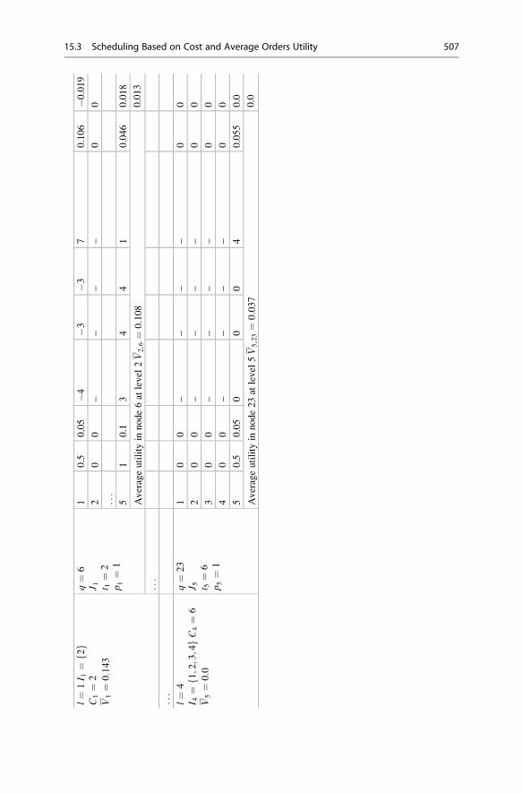
l¼
1I 1
¼2 fg
C1¼
2
V1¼
0:143
q¼
6
J 1 t 1¼
2
p1¼
1
10.5
0.05
�4�3
�37
0.106
�0.019
20
0–
––
–0
0
...
51
0.1
34
41
0.046
0.018
Averageutility
innode6at
level
2V2,6¼
0:108
0.013
...
...
l¼
4
I 4¼
1;2;3;4
fgC
4¼
6
V5¼
0:0
q¼
23
J 5 t 5¼
6
p5¼
1
10
0–
––
–0
0
20
0–
––
–0
0
30
0–
––
–0
0
40
0–
––
–0
0
50.5
0.05
00
04
0.055
0.0
Averageutility
innode23at
level
5V5,23¼
0:037
0.0
15.3 Scheduling Based on Cost and Average Orders Utility 507
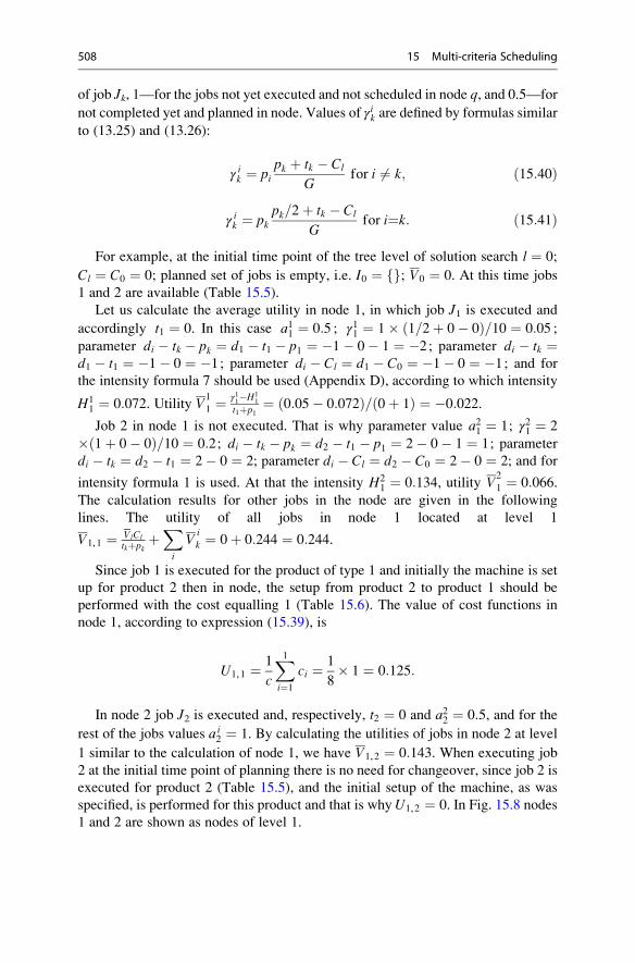
of job Jk, 1—for the jobs not yet executed and not scheduled in node q, and 0.5—for
not completed yet and planned in node. Values of γik are defined by formulas similar
to (13.25) and (13.26):
γ ik ¼ pipk þ tk � Cl
Gfor i 6¼ k; ð15:40Þ
γ ik ¼ pkpk=2þ tk � Cl
Gfor i¼k: ð15:41Þ
For example, at the initial time point of the tree level of solution search l ¼ 0;
Cl ¼ C0 ¼ 0; planned set of jobs is empty, i.e. I0 ¼ fg; V0 ¼ 0. At this time jobs
1 and 2 are available (Table 15.5).
Let us calculate the average utility in node 1, in which job J1 is executed and
accordingly t1 ¼ 0. In this case a11 ¼ 0:5 ; γ11 ¼ 1� 1=2þ 0� 0ð Þ=10 ¼ 0:05 ;parameter di � tk � pk ¼ d1 � t1 � p1 ¼ �1� 0� 1 ¼ �2 ; parameter di � tk ¼d1 � t1 ¼ �1� 0 ¼ �1 ; parameter di � Cl ¼ d1 � C0 ¼ �1� 0 ¼ �1 ; and for
the intensity formula 7 should be used (Appendix D), according to which intensity
H11 ¼ 0:072. Utility V
1
1 ¼ γ11�H1
1
t1þp1¼ 0:05� 0:072ð Þ= 0þ 1ð Þ ¼ �0:022.
Job 2 in node 1 is not executed. That is why parameter value a21 ¼ 1; γ21 ¼ 2
� 1þ 0� 0ð Þ=10 ¼ 0:2; di � tk � pk ¼ d2 � t1 � p1 ¼ 2� 0� 1 ¼ 1; parameter
di � tk ¼ d2 � t1 ¼ 2� 0 ¼ 2; parameter di � Cl ¼ d2 � C0 ¼ 2� 0 ¼ 2; and for
intensity formula 1 is used. At that the intensity H21 ¼ 0:134, utility V
2
1 ¼ 0:066.The calculation results for other jobs in the node are given in the following
lines. The utility of all jobs in node 1 located at level 1
V1,1 ¼ VlCl
tkþpkþXi
Vik ¼ 0þ 0:244 ¼ 0:244.
Since job 1 is executed for the product of type 1 and initially the machine is set
up for product 2 then in node, the setup from product 2 to product 1 should be
performed with the cost equalling 1 (Table 15.6). The value of cost functions in
node 1, according to expression (15.39), is
U1,1 ¼ 1
c
X1i¼1
ci ¼ 1
8� 1 ¼ 0:125:
In node 2 job J2 is executed and, respectively, t2 ¼ 0 and a22 ¼ 0:5, and for the
rest of the jobs values ai2 ¼ 1. By calculating the utilities of jobs in node 2 at level
1 similar to the calculation of node 1, we have V1,2 ¼ 0:143. When executing job
2 at the initial time point of planning there is no need for changeover, since job 2 is
executed for product 2 (Table 15.5), and the initial setup of the machine, as was
specified, is performed for this product and that is whyU1,2 ¼ 0. In Fig. 15.8 nodes
1 and 2 are shown as nodes of level 1.
508 15 Multi-criteria Scheduling
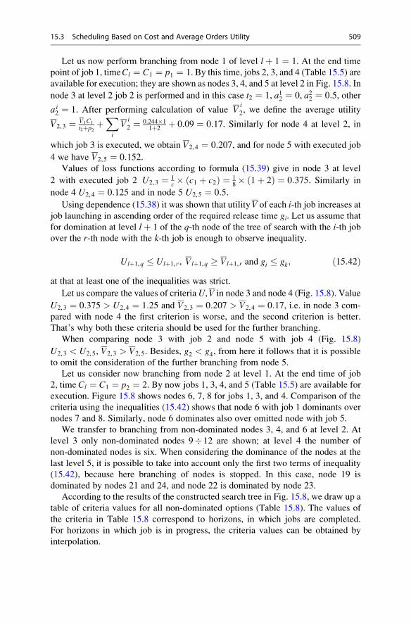
Let us now perform branching from node 1 of level lþ 1 ¼ 1. At the end time
point of job 1, timeCl ¼ C1 ¼ p1 ¼ 1. By this time, jobs 2, 3, and 4 (Table 15.5) are
available for execution; they are shown as nodes 3, 4, and 5 at level 2 in Fig. 15.8. In
node 3 at level 2 job 2 is performed and in this case t2 ¼ 1, a12 ¼ 0, a22 ¼ 0:5, other
ai2 ¼ 1. After performing calculation of value V
i2, we define the average utility
V2,3 ¼ V1C1
t2þp2þXi
Vi2 ¼ 0:244�1
1þ2þ 0:09 ¼ 0:17. Similarly for node 4 at level 2, in
which job 3 is executed, we obtain V2,4 ¼ 0:207, and for node 5 with executed job
4 we have V2,5 ¼ 0:152.Values of loss functions according to formula (15.39) give in node 3 at level
2 with executed job 2 U2,3 ¼ 1c � c1 þ c2ð Þ ¼ 1
8� 1þ 2ð Þ ¼ 0:375. Similarly in
node 4 U2,4 ¼ 0:125 and in node 5 U2,5 ¼ 0:5.
Using dependence (15.38) it was shown that utilityV of each i-th job increases atjob launching in ascending order of the required release time gi. Let us assume that
for domination at level lþ 1 of the q-th node of the tree of search with the i-th job
over the r-th node with the k-th job is enough to observe inequality.
Ulþ1,q � Ulþ1, r, Vlþ1,q � Vlþ1, r and gi � gk; ð15:42Þat that at least one of the inequalities was strict.
Let us compare the values of criteriaU,V in node 3 and node 4 (Fig. 15.8). Value
U2,3 ¼ 0:375 > U2,4 ¼ 1:25 and V2,3 ¼ 0:207 > V2,4 ¼ 0:17, i.e. in node 3 com-
pared with node 4 the first criterion is worse, and the second criterion is better.
That’s why both these criteria should be used for the further branching.
When comparing node 3 with job 2 and node 5 with job 4 (Fig. 15.8)
U2,3 < U2,5, V2,3 > V2,5. Besides, g2 < g4, from here it follows that it is possible
to omit the consideration of the further branching from node 5.
Let us consider now branching from node 2 at level 1. At the end time of job
2, time Cl ¼ C1 ¼ p2 ¼ 2. By now jobs 1, 3, 4, and 5 (Table 15.5) are available for
execution. Figure 15.8 shows nodes 6, 7, 8 for jobs 1, 3, and 4. Comparison of the
criteria using the inequalities (15.42) shows that node 6 with job 1 dominants over
nodes 7 and 8. Similarly, node 6 dominates also over omitted node with job 5.
We transfer to branching from non-dominated nodes 3, 4, and 6 at level 2. At
level 3 only non-dominated nodes 9� 12 are shown; at level 4 the number of
non-dominated nodes is six. When considering the dominance of the nodes at the
last level 5, it is possible to take into account only the first two terms of inequality
(15.42), because here branching of nodes is stopped. In this case, node 19 is
dominated by nodes 21 and 24, and node 22 is dominated by node 23.
According to the results of the constructed search tree in Fig. 15.8, we draw up a
table of criteria values for all non-dominated options (Table 15.8). The values of
the criteria in Table 15.8 correspond to horizons, in which jobs are completed.
For horizons in which job is in progress, the criteria values can be obtained by
interpolation.
15.3 Scheduling Based on Cost and Average Orders Utility 509
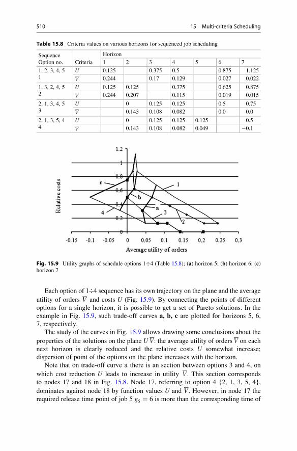
Each option of 1�4 sequence has its own trajectory on the plane and the averageutility of orders V and costs U (Fig. 15.9). By connecting the points of different
options for a single horizon, it is possible to get a set of Pareto solutions. In the
example in Fig. 15.9, such trade-off curves a, b, c are plotted for horizons 5, 6,
7, respectively.
The study of the curves in Fig. 15.9 allows drawing some conclusions about the
properties of the solutions on the plane U V: the average utility of orders V on each
next horizon is clearly reduced and the relative costs U somewhat increase;
dispersion of point of the options on the plane increases with the horizon.
Note that on trade-off curve а there is an section between options 3 and 4, on
which cost reduction U leads to increase in utility V. This section corresponds
to nodes 17 and 18 in Fig. 15.8. Node 17, referring to option 4 {2, 1, 3, 5, 4},
dominates against node 18 by function values U and V. However, in node 17 the
required release time point of job 5 g5 ¼ 6 is more than the corresponding time of
Table 15.8 Criteria values on various horizons for sequenced job scheduling
Sequence
Option no. Criteria
Horizon
1 2 3 4 5 6 7
1, 2, 3, 4, 5
1
U 0.125 0.375 0.5 0.875 1.125
V 0.244 0.17 0.129 0.027 0.022
1, 3, 2, 4, 5
2
U 0.125 0.125 0.375 0.625 0.875
V 0.244 0.207 0.115 0.019 0.015
2, 1, 3, 4, 5
3
U 0 0.125 0.125 0.5 0.75
V 0.143 0.108 0.082 0.0 0.0
2, 1, 3, 5, 4
4
U 0 0.125 0.125 0.125 0.5
V 0.143 0.108 0.082 0.049 �0.1
Fig. 15.9 Utility graphs of schedule options 1�4 (Table 15.8); (a) horizon 5; (b) horizon 6; (c)horizon 7
510 15 Multi-criteria Scheduling
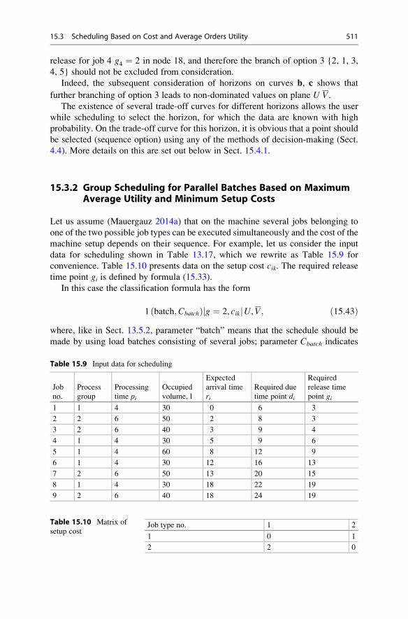
release for job 4 g4 ¼ 2 in node 18, and therefore the branch of option 3 {2, 1, 3,
4, 5} should not be excluded from consideration.
Indeed, the subsequent consideration of horizons on curves b, c shows that
further branching of option 3 leads to non-dominated values on plane U V.The existence of several trade-off curves for different horizons allows the user
while scheduling to select the horizon, for which the data are known with high
probability. On the trade-off curve for this horizon, it is obvious that a point should
be selected (sequence option) using any of the methods of decision-making (Sect.
4.4). More details on this are set out below in Sect. 15.4.1.
15.3.2 Group Scheduling for Parallel Batches Based on MaximumAverage Utility and Minimum Setup Costs
Let us assume (Mauergauz 2014a) that on the machine several jobs belonging to
one of the two possible job types can be executed simultaneously and the cost of the
machine setup depends on their sequence. For example, let us consider the input
data for scheduling shown in Table 13.17, which we rewrite as Table 15.9 for
convenience. Table 15.10 presents data on the setup cost cik. The required release
time point gi is defined by formula (15.33).
In this case the classification formula has the form
1 batch;Cbatchð Þ g ¼ 2, cikj jU,V; ð15:43Þwhere, like in Sect. 13.5.2, parameter “batch” means that the schedule should be
made by using load batches consisting of several jobs; parameter Cbatch indicates
Table 15.9 Input data for scheduling
Job
no.
Process
group
Processing
time pi
Occupied
volume, l
Expected
arrival time
ri
Required due
time point di
Required
release time
point gi
1 1 4 30 0 6 3
2 2 6 50 2 8 3
3 2 6 40 3 9 4
4 1 4 30 5 9 6
5 1 4 60 8 12 9
6 1 4 30 12 16 13
7 2 6 50 13 20 15
8 1 4 30 18 22 19
9 2 6 40 18 24 19
Table 15.10 Matrix of
setup costJob type no. 1 2
1 0 1
2 2 0
15.3 Scheduling Based on Cost and Average Orders Utility 511
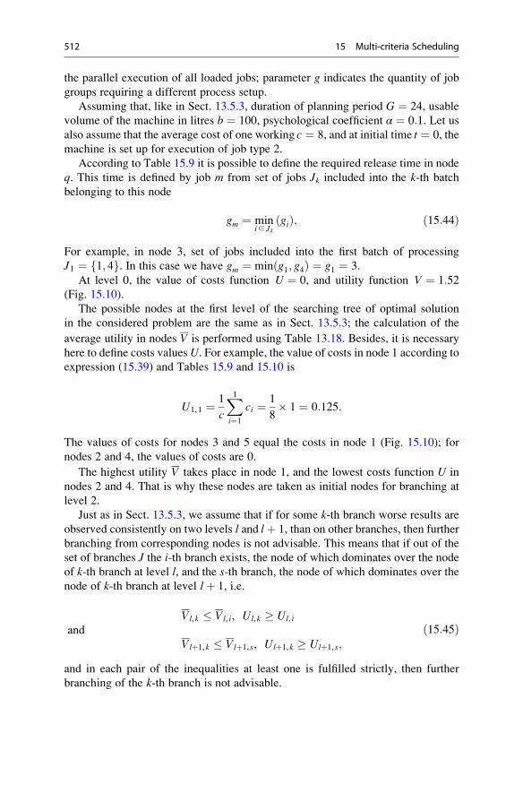
the parallel execution of all loaded jobs; parameter g indicates the quantity of job
groups requiring a different process setup.
Assuming that, like in Sect. 13.5.3, duration of planning period G ¼ 24, usable
volume of the machine in litres b ¼ 100, psychological coefficient α ¼ 0:1. Let usalso assume that the average cost of one working c ¼ 8, and at initial time t ¼ 0, the
machine is set up for execution of job type 2.
According to Table 15.9 it is possible to define the required release time in node
q. This time is defined by job m from set of jobs Jk included into the k-th batch
belonging to this node
gm ¼ mini∈ Jk
gið Þ; ð15:44Þ
For example, in node 3, set of jobs included into the first batch of processing
J1 ¼ 1; 4f g. In this case we have gm ¼ min g1; g4ð Þ ¼ g1 ¼ 3.
At level 0, the value of costs function U ¼ 0, and utility function V ¼ 1:52(Fig. 15.10).
The possible nodes at the first level of the searching tree of optimal solution
in the considered problem are the same as in Sect. 13.5.3; the calculation of the
average utility in nodes V is performed using Table 13.18. Besides, it is necessary
here to define costs values U. For example, the value of costs in node 1 according to
expression (15.39) and Tables 15.9 and 15.10 is
U1,1 ¼ 1
c
X1i¼1
ci ¼ 1
8� 1 ¼ 0:125:
The values of costs for nodes 3 and 5 equal the costs in node 1 (Fig. 15.10); for
nodes 2 and 4, the values of costs are 0.
The highest utility V takes place in node 1, and the lowest costs function U in
nodes 2 and 4. That is why these nodes are taken as initial nodes for branching at
level 2.
Just as in Sect. 13.5.3, we assume that if for some k-th branch worse results are
observed consistently on two levels l and lþ 1, than on other branches, then further
branching from corresponding nodes is not advisable. This means that if out of the
set of branches J the i-th branch exists, the node of which dominates over the node
of k-th branch at level l, and the s-th branch, the node of which dominates over the
node of k-th branch at level lþ 1, i.e.
Vl,k � Vl, i, Ul,k � Ul, i
and
Vlþ1,k � Vlþ1, s, Ulþ1,k � Ulþ1, s;
ð15:45Þ
and in each pair of the inequalities at least one is fulfilled strictly, then further
branching of the k-th branch is not advisable.
512 15 Multi-criteria Scheduling
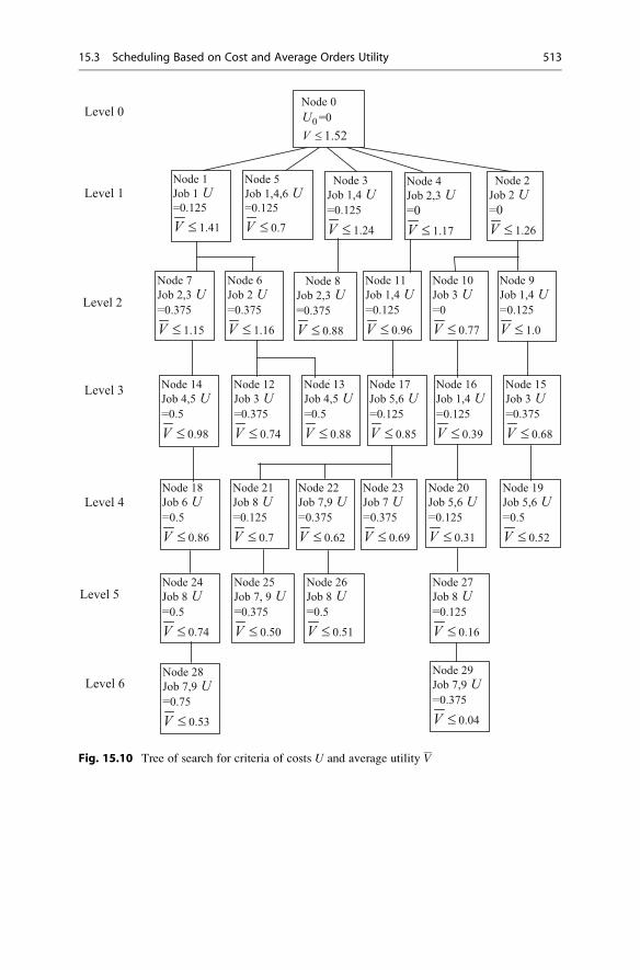
Level 5
Node 2
Job 2 U=0
V ≤ 1.26
Node 3
Job 1,4 U=0.125
V ≤ 1.24
Node 1
Job 1 U=0.125
V ≤ 1.41
Node 4
Job 2,3 U=0
V ≤ 1.17
Node 6
Job 2 U=0.375
V ≤ 1.16
Node 7
Job 2,3 U=0.375
V ≤ 1.15
Node 0
0U =0
V ≤ 1.52
Level 1
Level 0
Level 2
Node 12
Job 3 U=0.375
V ≤ 0.74
Level 3Node 15
Job 3 U=0.375
V ≤ 0.68
Level 4
Node 5
Job 1,4,6 U=0.125
V ≤ 0.7
Node 9
Job 1,4 U=0.125
V ≤ 1.0
Node 10
Job 3 U=0
V ≤ 0.77
Node 13
Job 4,5 U=0.5
V ≤ 0.88
Node 14
Job 4,5 U=0.5
V ≤ 0.98
Node 18
Job 6 U=0.5
V ≤ 0.86
Node 25
Job 7, 9 U=0.375
V ≤ 0.50
Node 26
Job 8 U=0.5
V ≤ 0.51
Level 6
Node 11
Job 1,4 U=0.125
V ≤ 0.96
Node 16
Job 1,4 U=0.125
V ≤ 0.39
Node 17
Job 5,6 U=0.125
V ≤ 0.85
Node 20
Job 5,6 U=0.125
V ≤ 0.31
Node 23
Job 7 U=0.375
V ≤ 0.69
Node 22
Job 7,9 U=0.375
V ≤ 0.62
Node 21
Job 8 U=0.125
V ≤ 0.7
Node 29
Job 7,9 U=0.375
V ≤ 0.04
Node 27
Job 8 U=0.125
V ≤ 0.16
Node 24
Job 8 U=0.5
V ≤ 0.74
Node 19
Job 5,6 U=0.5
V ≤ 0.52
Node 28
Job 7,9 U=0.75
V ≤ 0.53
Node 8
Job 2,3 U=0.375
V ≤ 0.88
Fig. 15.10 Tree of search for criteria of costs U and average utility V
15.3 Scheduling Based on Cost and Average Orders Utility 513
When branching from node 1, the load batches consisting of jobs {2}, {2, 3},
{4}, {4, 5} are possible and herewith the best option of utilityV is provided by node
6 at the second level with utility 1.16. Besides, as it was shown above in Sect.
13.5.3, it is necessary to take into account node 7 with jobs {2, 3}, since it give
better values V at the next level.
Values of criterion U in the nodes of the first level 1, 3, 5 are the same. That is
why for finding the need for branching from nodes 3 and 5 after branching from
node 1, we compare only values V on nodes 6 and 7 at the second level with the
corresponding valuesV in nodes 3 and 5. Obviously, that only branching from node
3 makes sense and the best results of branching occur for node 8.
As a result of this branching, it appears that at level 1 node 3 of branch {0, 3, 8}
is dominated by node 1 of branch {0, 1} and at level 2 is dominated by node 9 of
branch {0, 2, 9} and by node 11 of branch {0, 4, 11}. Hence, it appears that
according to (15.45) further branching from node 8 is not advisable.
Going to branching of nodes 2 and 4, at level 2 we obtain nodes 9, 10, 11. The
rest possible nodes are not shown, as they are further dominated by nodes 9, 10, 11.
At the third level we have six non-dominated nodes. With further branching, the
criteria values in nodes originating from 12 and 13 are dominated by the criteria
values in nodes 17 or 14, and so are not considered any more. Six non-dominated
nodes also exist at the fourth level and from nodes 14, 15, and 16 each of
non-dominated nodes 18, 19, and 20 originate, respectively, and from node 17—
three non-dominated nodes 21, 22, 23.
From branches {0, 4, 11, 17, 21, 25} and {0, 4, 11, 17, 22, 26}, the planning is
ended at level 5, i.e. to execute all scheduled jobs (Table 15.9) in this case it is
enough to consistently load five batches while branches {0, 1, 7, 14, 18, 24, 2} and
{0, 2, 10, 16, 20, 27, 29} provide six load batches.
To demonstrate the dependence of the criteria values from the sequence of jobs,
we compare, for example, the criteria values in nodes 15 and 16. Upon execution of
jobs in these nodes, it appears that same jobs 1, 2, 3, and 4 are executed; however,
the criteria values are very different.
According to the results of construction of the searching tree in Fig. 15.10, we
draw up a table of criteria values on each horizon for all non-dominated options
(Table 15.11).
The execution time points of the jobs in the nodes of the searching tree do not
always coincide with the values of the horizons in Table 15.11. In such cases, it is
possible to refer the execution time point to the larger or smaller horizon using the
rule:
with hiþ1 > Cl � hi þ hi þ hiþ1
2refer execution to h ¼ hiþ1;
with hiþ1 > Cl < hi þ hi þ hiþ1
2refer execution to h ¼ hi: ð15:46Þ
For example for node 7 Cl ¼ 10 and assume that horizon h ¼ 12.
514 15 Multi-criteria Scheduling
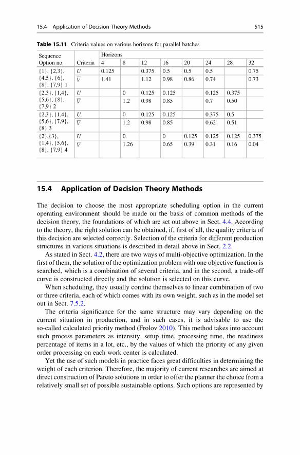
15.4 Application of Decision Theory Methods
The decision to choose the most appropriate scheduling option in the current
operating environment should be made on the basis of common methods of the
decision theory, the foundations of which are set out above in Sect. 4.4. According
to the theory, the right solution can be obtained, if, first of all, the quality criteria of
this decision are selected correctly. Selection of the criteria for different production
structures in various situations is described in detail above in Sect. 2.2.
As stated in Sect. 4.2, there are two ways of multi-objective optimization. In the
first of them, the solution of the optimization problem with one objective function is
searched, which is a combination of several criteria, and in the second, a trade-off
curve is constructed directly and the solution is selected on this curve.
When scheduling, they usually confine themselves to linear combination of two
or three criteria, each of which comes with its own weight, such as in the model set
out in Sect. 7.5.2.
The criteria significance for the same structure may vary depending on the
current situation in production, and in such cases, it is advisable to use the
so-called calculated priority method (Frolov 2010). This method takes into account
such process parameters as intensity, setup time, processing time, the readiness
percentage of items in a lot, etc., by the values of which the priority of any given
order processing on each work center is calculated.
Yet the use of such models in practice faces great difficulties in determining the
weight of each criterion. Therefore, the majority of current researches are aimed at
direct construction of Pareto solutions in order to offer the planner the choice from a
relatively small set of possible sustainable options. Such options are represented by
Table 15.11 Criteria values on various horizons for parallel batches
Sequence
Option no. Criteria
Horizons
4 8 12 16 20 24 28 32
{1}, {2,3},
{4,5}, {6},
{8}, {7,9} 1
U 0.125 0.375 0.5 0.5 0.5 0.75
V 1.41 1.12 0.98 0.86 0.74 0.73
{2,3}, {1,4},
{5,6}, {8},
{7,9} 2
U 0 0.125 0.125 0.125 0.375
V 1.2 0.98 0.85 0.7 0.50
{2,3}, {1,4},
{5,6}, {7,9},
{8} 3
U 0 0.125 0.125 0.375 0.5
V 1.2 0.98 0.85 0.62 0.51
{2},{3},
{1,4}, {5,6},
{8}, {7,9} 4
U 0 0 0.125 0.125 0.125 0.375
V 1.26 0.65 0.39 0.31 0.16 0.04
15.4 Application of Decision Theory Methods 515
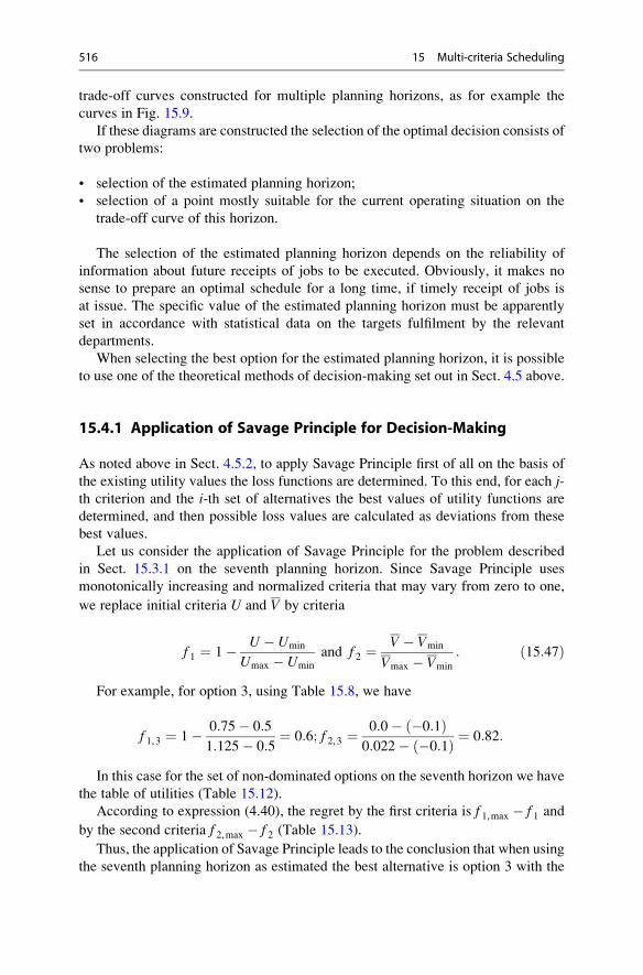
trade-off curves constructed for multiple planning horizons, as for example the
curves in Fig. 15.9.
If these diagrams are constructed the selection of the optimal decision consists of
two problems:
• selection of the estimated planning horizon;
• selection of a point mostly suitable for the current operating situation on the
trade-off curve of this horizon.
The selection of the estimated planning horizon depends on the reliability of
information about future receipts of jobs to be executed. Obviously, it makes no
sense to prepare an optimal schedule for a long time, if timely receipt of jobs is
at issue. The specific value of the estimated planning horizon must be apparently
set in accordance with statistical data on the targets fulfilment by the relevant
departments.
When selecting the best option for the estimated planning horizon, it is possible
to use one of the theoretical methods of decision-making set out in Sect. 4.5 above.
15.4.1 Application of Savage Principle for Decision-Making
As noted above in Sect. 4.5.2, to apply Savage Principle first of all on the basis of
the existing utility values the loss functions are determined. To this end, for each j-th criterion and the i-th set of alternatives the best values of utility functions are
determined, and then possible loss values are calculated as deviations from these
best values.
Let us consider the application of Savage Principle for the problem described
in Sect. 15.3.1 on the seventh planning horizon. Since Savage Principle uses
monotonically increasing and normalized criteria that may vary from zero to one,
we replace initial criteria U and V by criteria
f 1 ¼ 1� U � Umin
Umax � Umin
and f 2 ¼V � Vmin
Vmax � Vmin
: ð15:47Þ
For example, for option 3, using Table 15.8, we have
f 1,3 ¼ 1� 0:75� 0:5
1:125� 0:5¼ 0:6; f 2,3 ¼
0:0� �0:1ð Þ0:022� �0:1ð Þ ¼ 0:82:
In this case for the set of non-dominated options on the seventh horizon we have
the table of utilities (Table 15.12).
According to expression (4.40), the regret by the first criteria is f 1,max � f 1 and
by the second criteria f 2,max � f 2 (Table 15.13).
Thus, the application of Savage Principle leads to the conclusion that when using
the seventh planning horizon as estimated the best alternative is option 3 with the
516 15 Multi-criteria Scheduling
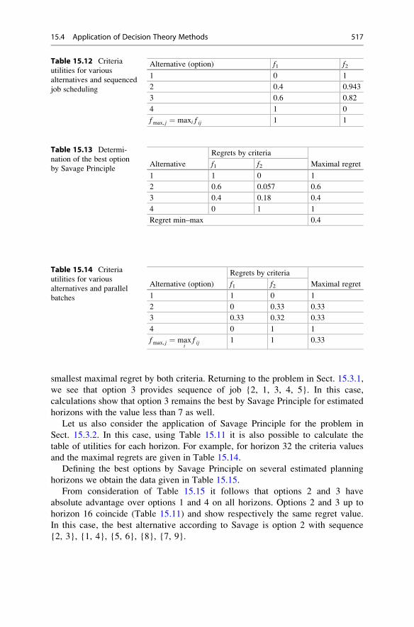
smallest maximal regret by both criteria. Returning to the problem in Sect. 15.3.1,
we see that option 3 provides sequence of job {2, 1, 3, 4, 5}. In this case,
calculations show that option 3 remains the best by Savage Principle for estimated
horizons with the value less than 7 as well.
Let us also consider the application of Savage Principle for the problem in
Sect. 15.3.2. In this case, using Table 15.11 it is also possible to calculate the
table of utilities for each horizon. For example, for horizon 32 the criteria values
and the maximal regrets are given in Table 15.14.
Defining the best options by Savage Principle on several estimated planning
horizons we obtain the data given in Table 15.15.
From consideration of Table 15.15 it follows that options 2 and 3 have
absolute advantage over options 1 and 4 on all horizons. Options 2 and 3 up to
horizon 16 coincide (Table 15.11) and show respectively the same regret value.
In this case, the best alternative according to Savage is option 2 with sequence
{2, 3}, {1, 4}, {5, 6}, {8}, {7, 9}.
Table 15.12 Criteria
utilities for various
alternatives and sequenced
job scheduling
Alternative (option) f1 f2
1 0 1
2 0.4 0.943
3 0.6 0.82
4 1 0
fmax, j ¼ maxi f ij 1 1
Table 15.13 Determi-
nation of the best option
by Savage PrincipleAlternative
Regrets by criteria
Maximal regretf1 f2
1 1 0 1
2 0.6 0.057 0.6
3 0.4 0.18 0.4
4 0 1 1
Regret min–max 0.4
Table 15.14 Criteria
utilities for various
alternatives and parallel
batches
Alternative (option)
Regrets by criteria
Maximal regretf1 f2
1 1 0 1
2 0 0.33 0.33
3 0.33 0.32 0.33
4 0 1 1
fmax, j ¼ maxi
f ij 1 1 0.33
15.4 Application of Decision Theory Methods 517
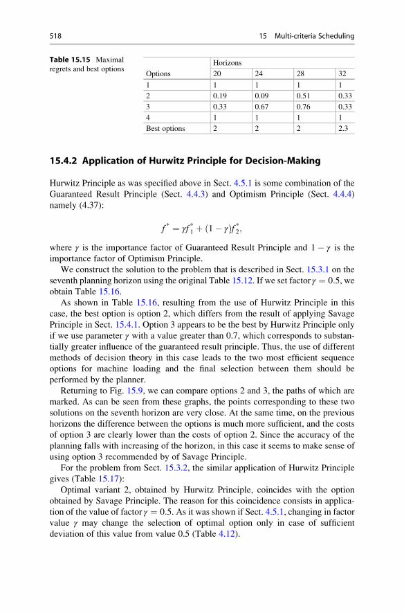
15.4.2 Application of Hurwitz Principle for Decision-Making
Hurwitz Principle as was specified above in Sect. 4.5.1 is some combination of the
Guaranteed Result Principle (Sect. 4.4.3) and Optimism Principle (Sect. 4.4.4)
namely (4.37):
f * ¼ γf *1 þ 1� γð Þf *2;where γ is the importance factor of Guaranteed Result Principle and 1� γ is the
importance factor of Optimism Principle.
We construct the solution to the problem that is described in Sect. 15.3.1 on the
seventh planning horizon using the original Table 15.12. If we set factor γ ¼ 0:5, weobtain Table 15.16.
As shown in Table 15.16, resulting from the use of Hurwitz Principle in this
case, the best option is option 2, which differs from the result of applying Savage
Principle in Sect. 15.4.1. Option 3 appears to be the best by Hurwitz Principle only
if we use parameter γ with a value greater than 0.7, which corresponds to substan-
tially greater influence of the guaranteed result principle. Thus, the use of different
methods of decision theory in this case leads to the two most efficient sequence
options for machine loading and the final selection between them should be
performed by the planner.
Returning to Fig. 15.9, we can compare options 2 and 3, the paths of which are
marked. As can be seen from these graphs, the points corresponding to these two
solutions on the seventh horizon are very close. At the same time, on the previous
horizons the difference between the options is much more sufficient, and the costs
of option 3 are clearly lower than the costs of option 2. Since the accuracy of the
planning falls with increasing of the horizon, in this case it seems to make sense of
using option 3 recommended by of Savage Principle.
For the problem from Sect. 15.3.2, the similar application of Hurwitz Principle
gives (Table 15.17):
Optimal variant 2, obtained by Hurwitz Principle, coincides with the option
obtained by Savage Principle. The reason for this coincidence consists in applica-
tion of the value of factor γ ¼ 0:5. As it was shown if Sect. 4.5.1, changing in factorvalue γ may change the selection of optimal option only in case of sufficient
deviation of this value from value 0.5 (Table 4.12).
Table 15.15 Maximal
regrets and best optionsOptions
Horizons
20 24 28 32
1 1 1 1 1
2 0.19 0.09 0.51 0.33
3 0.33 0.67 0.76 0.33
4 1 1 1 1
Best options 2 2 2 2.3
518 15 Multi-criteria Scheduling
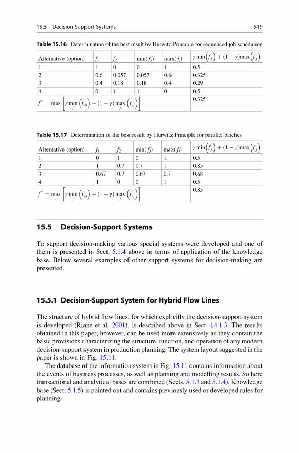
15.5 Decision-Support Systems
To support decision-making various special systems were developed and one of
them is presented in Sect. 5.1.4 above in terms of application of the knowledge
base. Below several examples of other support systems for decision-making are
presented.
15.5.1 Decision-Support System for Hybrid Flow Lines
The structure of hybrid flow lines, for which explicitly the decision-support system
is developed (Riane et al. 2001), is described above in Sect. 14.1.3. The results
obtained in this paper, however, can be used more extensively as they contain the
basic provisions characterizing the structure, function, and operation of any modern
decision-support system in production planning. The system layout suggested in the
paper is shown in Fig. 15.11.
The database of the information system in Fig. 15.11 contains information about
the events of business processes, as well as planning and modelling results. So here
transactional and analytical bases are combined (Sects. 5.1.3 and 5.1.4). Knowledge
base (Sect. 5.1.5) is pointed out and contains previously used or developed rules for
planning.
Table 15.16 Determination of the best result by Hurwitz Principle for sequenced job scheduling
Alternative (option) f1 f2 min( fj) max( fj)γmin f j
� �þ 1� γð Þmax f j
� �1 1 0 0 1 0.5
2 0.6 0.057 0.057 0.6 0.325
3 0.4 0.18 0.18 0.4 0.29
4 0 1 1 0 0.5
f * ¼ maxi
γminj
f ij
� �þ 1� γð Þmax
jf ij
� � �0.325
Table 15.17 Determination of the best result by Hurwitz Principle for parallel batches
Alternative (option) f1 f2 min( fj) max( fj)γmin f j
� �þ 1� γð Þmax f j
� �1 0 1 0 1 0.5
2 1 0.7 0.7 1 0.85
3 0.67 0.7 0.67 0.7 0.68
4 1 0 0 1 0.5
f * ¼ maxi
γminj
f ij
� �þ 1� γð Þmax
jf ij
� � �0.85
15.5 Decision-Support Systems 519
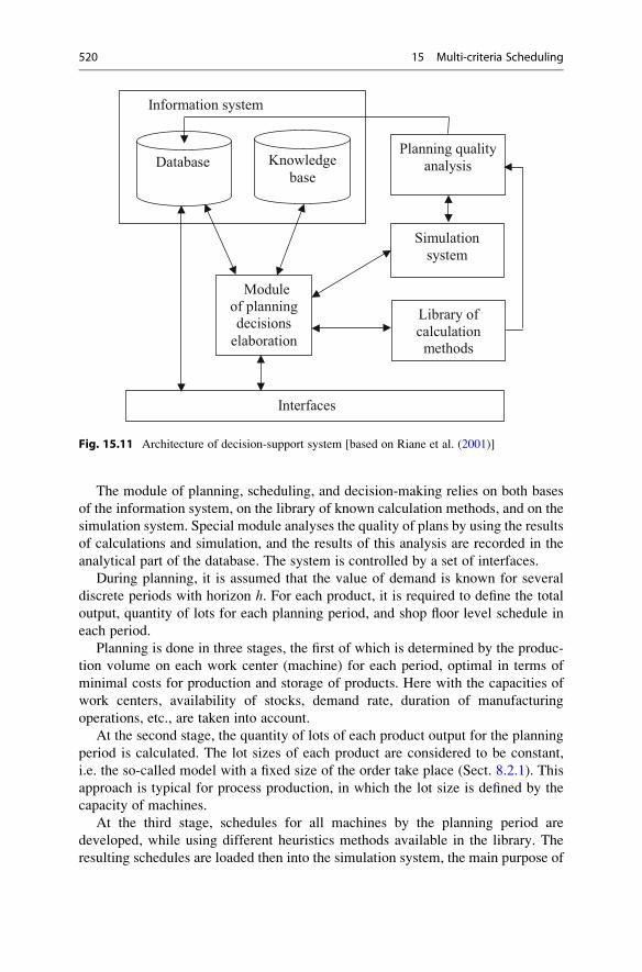
The module of planning, scheduling, and decision-making relies on both bases
of the information system, on the library of known calculation methods, and on the
simulation system. Special module analyses the quality of plans by using the results
of calculations and simulation, and the results of this analysis are recorded in the
analytical part of the database. The system is controlled by a set of interfaces.
During planning, it is assumed that the value of demand is known for several
discrete periods with horizon h. For each product, it is required to define the total
output, quantity of lots for each planning period, and shop floor level schedule in
each period.
Planning is done in three stages, the first of which is determined by the produc-
tion volume on each work center (machine) for each period, optimal in terms of
minimal costs for production and storage of products. Here with the capacities of
work centers, availability of stocks, demand rate, duration of manufacturing
operations, etc., are taken into account.
At the second stage, the quantity of lots of each product output for the planning
period is calculated. The lot sizes of each product are considered to be constant,
i.e. the so-called model with a fixed size of the order take place (Sect. 8.2.1). This
approach is typical for process production, in which the lot size is defined by the
capacity of machines.
At the third stage, schedules for all machines by the planning period are
developed, while using different heuristics methods available in the library. The
resulting schedules are loaded then into the simulation system, the main purpose of
Information system
Interfaces
Module of planning decisions
elaboration
Database Knowledge
base
Library of calculation methods
Simulation system
Planning quality analysis
Fig. 15.11 Architecture of decision-support system [based on Riane et al. (2001)]
520 15 Multi-criteria Scheduling
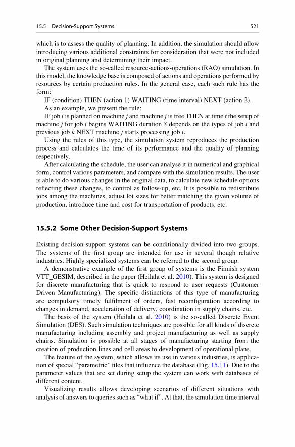
which is to assess the quality of planning. In addition, the simulation should allow
introducing various additional constraints for consideration that were not included
in original planning and determining their impact.
The system uses the so-called resource-actions-operations (RAO) simulation. In
this model, the knowledge base is composed of actions and operations performed by
resources by certain production rules. In the general case, each such rule has the
form:
IF (condition) THEN (action 1) WAITING (time interval) NEXT (action 2).
As an example, we present the rule:
IF job i is planned on machine j and machine j is free THEN at time t the setup ofmachine j for job i begins WAITING duration S depends on the types of job i andprevious job k NEXT machine j starts processing job i.
Using the rules of this type, the simulation system reproduces the production
process and calculates the time of its performance and the quality of planning
respectively.
After calculating the schedule, the user can analyse it in numerical and graphical
form, control various parameters, and compare with the simulation results. The user
is able to do various changes in the original data, to calculate new schedule options
reflecting these changes, to control as follow-up, etc. It is possible to redistribute
jobs among the machines, adjust lot sizes for better matching the given volume of
production, introduce time and cost for transportation of products, etc.
15.5.2 Some Other Decision-Support Systems
Existing decision-support systems can be conditionally divided into two groups.
The systems of the first group are intended for use in several though relative
industries. Highly specialized systems can be referred to the second group.
A demonstrative example of the first group of systems is the Finnish system
VTT_GESIM, described in the paper (Heilala et al. 2010). This system is designed
for discrete manufacturing that is quick to respond to user requests (Customer
Driven Manufacturing). The specific distinctions of this type of manufacturing
are compulsory timely fulfilment of orders, fast reconfiguration according to
changes in demand, acceleration of delivery, coordination in supply chains, etc.
The basis of the system (Heilala et al. 2010) is the so-called Discrete Event
Simulation (DES). Such simulation techniques are possible for all kinds of discrete
manufacturing including assembly and project manufacturing as well as supply
chains. Simulation is possible at all stages of manufacturing starting from the
creation of production lines and cell areas to development of operational plans.
The feature of the system, which allows its use in various industries, is applica-
tion of special “parametric” files that influence the database (Fig. 15.11). Due to the
parameter values that are set during setup the system can work with databases of
different content.
Visualizing results allows developing scenarios of different situations with
analysis of answers to queries such as “what if”. At that, the simulation time interval
15.5 Decision-Support Systems 521
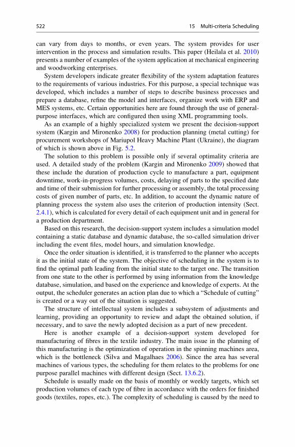
can vary from days to months, or even years. The system provides for user
intervention in the process and simulation results. This paper (Heilala et al. 2010)
presents a number of examples of the system application at mechanical engineering
and woodworking enterprises.
System developers indicate greater flexibility of the system adaptation features
to the requirements of various industries. For this purpose, a special technique was
developed, which includes a number of steps to describe business processes and
prepare a database, refine the model and interfaces, organize work with ERP and
MES systems, etc. Certain opportunities here are found through the use of general-
purpose interfaces, which are configured then using XML programming tools.
As an example of a highly specialized system we present the decision-support
system (Kargin and Mironenko 2008) for production planning (metal cutting) for
procurement workshops of Mariupol Heavy Machine Plant (Ukraine), the diagram
of which is shown above in Fig. 5.2.
The solution to this problem is possible only if several optimality criteria are
used. A detailed study of the problem (Kargin and Mironenko 2009) showed that
these include the duration of production cycle to manufacture a part, equipment
downtime, work-in-progress volumes, costs, delaying of parts to the specified date
and time of their submission for further processing or assembly, the total processing
costs of given number of parts, etc. In addition, to account the dynamic nature of
planning process the system also uses the criterion of production intensity (Sect.
2.4.1), which is calculated for every detail of each equipment unit and in general for
a production department.
Based on this research, the decision-support system includes a simulation model
containing a static database and dynamic database, the so-called simulation driver
including the event files, model hours, and simulation knowledge.
Once the order situation is identified, it is transferred to the planner who accepts
it as the initial state of the system. The objective of scheduling in the system is to
find the optimal path leading from the initial state to the target one. The transition
from one state to the other is performed by using information from the knowledge
database, simulation, and based on the experience and knowledge of experts. At the
output, the scheduler generates an action plan due to which a “Schedule of cutting”
is created or a way out of the situation is suggested.
The structure of intellectual system includes a subsystem of adjustments and
learning, providing an opportunity to review and adapt the obtained solution, if
necessary, and to save the newly adopted decision as a part of new precedent.
Here is another example of a decision-support system developed for
manufacturing of fibres in the textile industry. The main issue in the planning of
this manufacturing is the optimization of operation in the spinning machines area,
which is the bottleneck (Silva and Magalhaes 2006). Since the area has several
machines of various types, the scheduling for them relates to the problems for one
purpose parallel machines with different design (Sect. 13.6.2).
Schedule is usually made on the basis of monthly or weekly targets, which set
production volumes of each type of fibre in accordance with the orders for finished
goods (textiles, ropes, etc.). The complexity of scheduling is caused by the need to
522 15 Multi-criteria Scheduling

consider two mutually contradictory criteria: cost of setups and just-in-time fulfil-
ment of targets, i.e. the problem under consideration in this aspect is similar to the
problem described above in Sect. 15.3.1.
However, in reality, the real problem stated in the paper (Silva and Magalhaes
2006) is much more complicated, because its solution is imposed with a number of
additional constraints. In particular, in addition to the need to consider the relation
of the setup cost to the sequence of jobs, it is also necessary to take into account the
wearing degree of the jets through which the yarns are pulled, as well as the
possibility to use the machines only for certain types of yarns, different capacities
of the machines, etc.
In this paper on the basis of the Discrete Lot sizing and Scheduling Problem
(DLSP) described above in Sect. 11.1.4, a special scheduling algorithm for multiple
parallel different machines is developed. However, the use of this algorithm to
develop a satisfactory schedule was insufficient, and further the optimization
algorithm was used as a part of the decision-support system. This system also
included a database and a user interface. Further development of this system (Silva
2009) based on specialized software tool enables the planner to use background
experience (knowledge base) in order to adjust the result of the calculations and
verify own decisions on the model.
In some cases, it is advisable to use relatively simple systems that can be called
decision-support tools. In the paper of Buehlmann et al. (2000), a simple decision-
support system for the production of wood panels is given. The system includes MS
Excel forms, by which the user in the workshop can optimize the schedule in case of
changes in delivery time and prices of materials produced. For the job shop
manufacturing, such decision-support tool using MS Excel and the techniques
described above in Sect. 15.3 is described in the paper of Mauergauz (2014b).
References
Bourgade, V., Aguilera, L. M., Penz, B., & Binder, Z. (1995). Probleme industriel
d’ordonnancement bicritere sur machine unique : modelisation et aide a la decision. R.A.I.R.O., 29, 869–883.
Buehlmann, U., Ragsdale, C. T., & Gfeller, B. (2000). A spreadsheet-based decision support
system for wood panel manufacturing. Decision Support Systems, 28, 207–227.Daniels, R. L., & Chambers, R. J. (1990). Multi-objective flow-shop scheduling. Naval Research
Logistics, 37, 981–995.Frolov, Y. B. (2010). Management of machine systems: Modern management concepts in produc-
tion logistics. Machine-Tool Fleet, 6, 41–43 (in Russian).
Garey, M. R., Targian, R. E., & Wilfong, G. T. (1988). One-processor scheduling with symmetric
earliness and tardiness penalties. Mathematics of Operations Research, 13, 330–348.Heilala, J., Montonen, J., Jarvinen, P., & Kivikunnas, S. (2010). Decision support using simulation
for customer-driven manufacturing system design and operations planning. In Advances indecision support systems. INTECH, Croatia.
Kargin, A. A., & Mironenko, D. S. (2008). Experience of production planning automation at OJSC
“MZTM”. Bulletin of Donetsk National University, Series A: Natural Science, 2, 517–521(in Russian).
References 523
Kargin, A. A., & Mironenko, D. S. (2009). Conceptual and algorithmic model of simulation
system of production (metal cutting) in the procurement workshops at OJSC “MZTM”.
Bulletin of Donetsk National University, Series A: Natural Science, 1, 452–457 (in Russian).
Lin, K. S. (1983). Hybrid algorithm for sequencing with bicriteria. Journal of Optimization Theoryand Applications, 39, 105–124.
Mauergauz, Y. E. (2013). Cost-efficiency method for production scheduling (pp. 587–593).
Proceedings of the World Congress on Engineering, London.
Mauergauz, Y. E. (2014a). Dynamic Pareto-optimal group scheduling for a single machine.
International Journal of Industrial and Systems Engineering, 16, 537–559.Mauergauz, Y. E. (2014b). Decision support tool for group job-shop scheduling problems
(pp. 397–406). Proceedings of the 4th International Conference on Simulation and Modelling,
Methodologies, Technologies and Applications, Vienna.
McCormick, S. T., & Pinedo, M. L. (1995). Scheduling n independent jobs onm uniform machines
with both flow-time and makespan objectives: a parametric analysis. ORSA Journal onComputing, 7, 63–77.
Mohri, S., Masuda, T., & Ishii, H. (1999). Bi-criteria scheduling problem on three identical parallel
machines. International Journal of Production Economics, 60–61, 529–536.Nagar, A., Heragu, S. S., & Haddock, J. (1995). A branch-and-bound approach for a two-machine
flowshop scheduling problem. Journal of Operational Research Society, 46, 721–734.Parveen, S., & Ullah, H. (2010). Review on job-shop and flow-shop scheduling using multicriteria
decision making. Journal of Mechanical Engineering, 41, 130–146.Riane, F., Artiba, A., & Iassinovski, S. (2001). An integrated production planning and scheduling
system for hybrid flowshop organizations. http://isiarticles.com/bundles/Article/pre/pdf/5544.
Silva, C. (2009). Combining ad hoc decision-making behaviour with formal planning and sched-
uling rules: A case study in the synthetic fibre production industry. Production Planning &Control, 20, 635–648.
Silva, C., & Magalhaes, J. M. (2006). Heuristic lot size scheduling on unrelated parallel machines
with applications in the textile industry. Computers & Industrial Engineering, 50, 76–89.Sivrikaya-Serifoglu, F. S., & Ulusoy, G. (1998). A bicriteria two machine permutation flowshop
problem. European Journal of Operational Research, 107, 414–430.Sundararaghavan, P. S., & Ahmed, M. U. (1984). Minimizing the sun of absolute lateness in
single-machine and multimachine scheduling. Naval Research Logistics Quarterly, 31,325–333.
T’Kindt, V., & Billaut, J. C. (2005). Multicriteria scheduling. Theory, models and algorithms.Berlin: Springer.
VanWassenhoven, L., & Gelders, L. F. (1980). Solving a bicriterion scheduling problem.
European Journal of Operational Research, 4, 42–48.
524 15 Multi-criteria Scheduling
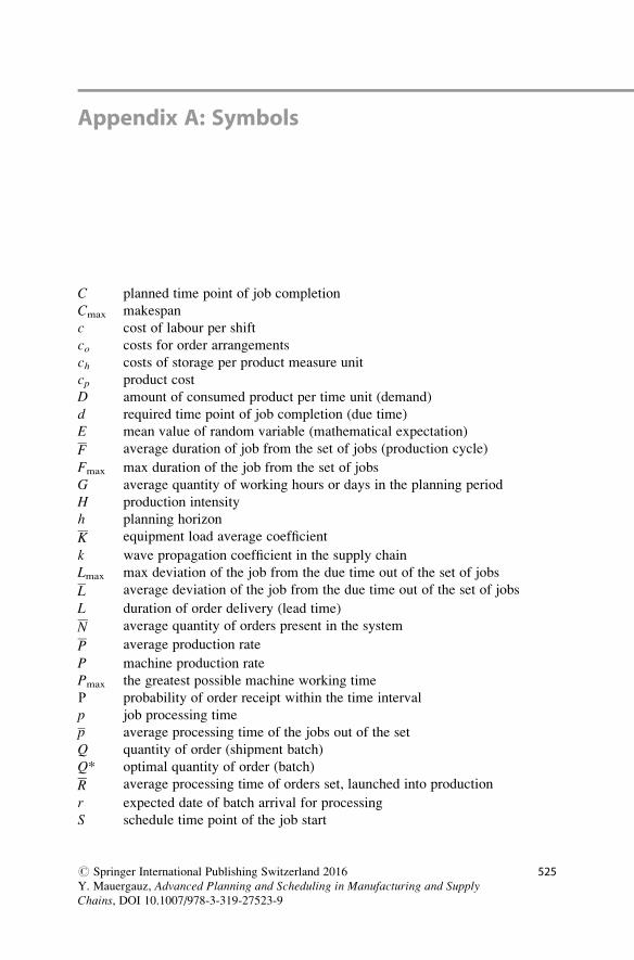
Appendix A: Symbols
C planned time point of job completion
Cmax makespan
c cost of labour per shift
co costs for order arrangements
ch costs of storage per product measure unit
cp product cost
D amount of consumed product per time unit (demand)
d required time point of job completion (due time)
E mean value of random variable (mathematical expectation)
F average duration of job from the set of jobs (production cycle)
Fmax max duration of the job from the set of jobs
G average quantity of working hours or days in the planning period
H production intensity
h planning horizon
K equipment load average coefficient
k wave propagation coefficient in the supply chain
Lmax max deviation of the job from the due time out of the set of jobs
L average deviation of the job from the due time out of the set of jobs
L duration of order delivery (lead time)
N average quantity of orders present in the system
P average production rate
P machine production rate
Pmax the greatest possible machine working time
Ρ probability of order receipt within the time interval
p job processing time
p average processing time of the jobs out of the set
Q quantity of order (shipment batch)
Q* optimal quantity of order (batch)
R average processing time of orders set, launched into production
r expected date of batch arrival for processing
S schedule time point of the job start
# Springer International Publishing Switzerland 2016
Y. Mauergauz, Advanced Planning and Scheduling in Manufacturing and SupplyChains, DOI 10.1007/978-3-319-27523-9
525

SL service level_S upper level of the stock
s setup time
_s quantity of stock at the reorder point
Tmax max job tardiness out of the job set
T average job tardiness out of the job set
T cycle (period) time of shipment
U function of negative utility of costs (loss function)
V function of current order utility
V function of average orders utility
W average production workload
w average queuing time of order
w job weighting factor
Y alternative version
Z current stock
Zc safety stock
α psychological coefficient
δ binary variable
ε effective point neighbourhood (distance from the trade-off curve)
σ standard deviation of a random variable from its mean value
κ safety factor (factor of accounting the spread in values of random function)
ƛ Lagrange multiplier
λ mean rate of incoming orders in the system (demand)
χ correction factor for the optimal batch size
η readiness percentage of operation
v variation coefficient of a random variable
Π expected profit
τ processing time of one part
ω frequency of a product in one schedule cycle
Ω orders frequency
526 Appendix A: Symbols
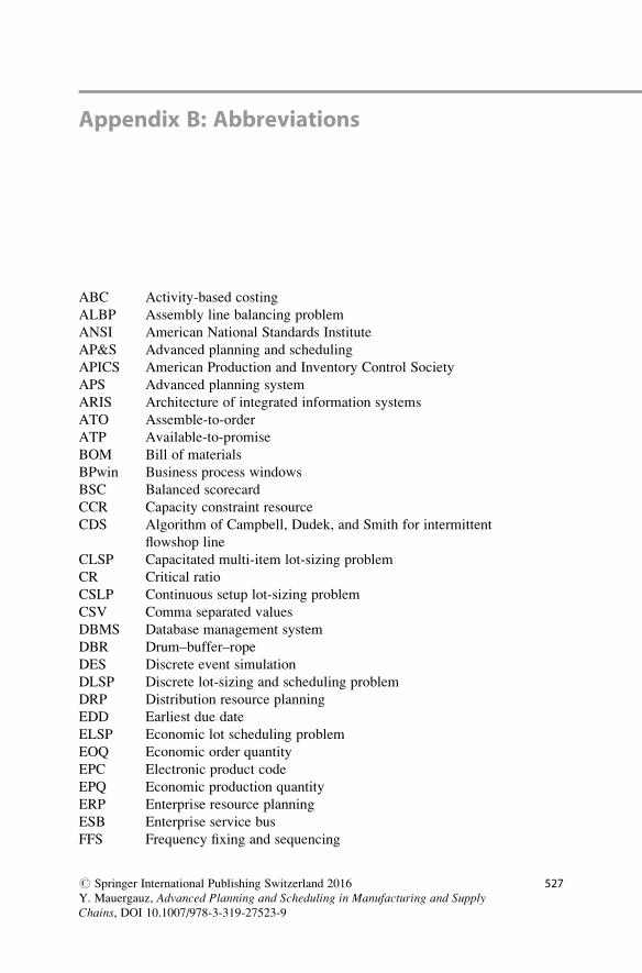
Appendix B: Abbreviations
ABC Activity-based costing
ALBP Assembly line balancing problem
ANSI American National Standards Institute
AP&S Advanced planning and scheduling
APICS American Production and Inventory Control Society
APS Advanced planning system
ARIS Architecture of integrated information systems
ATO Assemble-to-order
ATP Available-to-promise
BOM Bill of materials
BPwin Business process windows
BSC Balanced scorecard
CCR Capacity constraint resource
CDS Algorithm of Campbell, Dudek, and Smith for intermittent
flowshop line
CLSP Capacitated multi-item lot-sizing problem
CR Critical ratio
CSLP Continuous setup lot-sizing problem
CSV Comma separated values
DBMS Database management system
DBR Drum–buffer–rope
DES Discrete event simulation
DLSP Discrete lot-sizing and scheduling problem
DRP Distribution resource planning
EDD Earliest due date
ELSP Economic lot scheduling problem
EOQ Economic order quantity
EPC Electronic product code
EPQ Economic production quantity
ERP Enterprise resource planning
ESB Enterprise service bus
FFS Frequency fixing and sequencing
# Springer International Publishing Switzerland 2016
Y. Mauergauz, Advanced Planning and Scheduling in Manufacturing and SupplyChains, DOI 10.1007/978-3-319-27523-9
527
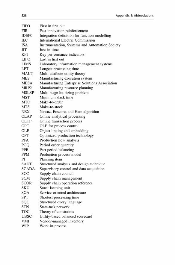
FIFO First in first out
FIR Fast innovation reinforcement
IDEF0 Integration definition for function modelling
IEC International Electric Commission
ISA Instrumentation, Systems and Automation Society
JIT Just-in-time
KPI Key performance indicators
LIFO Last in first out
LIMS Laboratory information management systems
LPT Longest processing time
MAUT Multi-attribute utility theory
MES Manufacturing execution system
MESA Manufacturing Enterprise Solutions Association
MRP2 Manufacturing resource planning
MSLSP Multi-stage lot-sizing problem
MST Minimum slack time
MTO Make-to-order
MTS Make-to-stock
NEX Nawaz, Enscore, and Ham algorithm
OLAP Online analytical processing
OLTP Online transaction process
OPC OLE for process control
OLE Object linking and embedding
OPT Optimized production technology
PFA Production flow analysis
POQ Period order quantity
PPB Part period balancing
PPM Production process model
PI Planning item
SADT Structured analysis and design technique
SCADA Supervisory control and data acquisition
SCC Supply chain council
SCM Supply chain management
SCOR Supply chain operation reference
SKU Stock-keeping unit
SOA Service-oriented architecture
SPT Shortest processing time
SQL Structured query language
STN State-task network
TOC Theory of constraints
UBSC Utility-based balanced scorecard
VMI Vendor-managed inventory
WIP Work-in-process
528 Appendix B: Abbreviations
Appendix C: Classification Parametersof Schedules
Classification (2.13) of form α | β | γ is of great importance in ordering the
scheduling problems. The classification has fields with three directions: type of
production (type of machines used), type of jobs performed and various constraints,
and type of objective function.
C.1 Parameters in Field a
These parameters have the structure of type α1α2(α3), i.e. often consist of two and
sometime three elements. The list of possible values α1 is presented below.
empty value in field α1 means that a single machine is under consideration;
α1 ¼ P parallel identical machines
α1 ¼ Q parallel uniform machines
α1 ¼ R parallel unrelated machines
α1 ¼ F flowshop production
α1 ¼ J jobshop production
α1 ¼ O openshop production.
Symbol α2 serves to describe the quantity of machines. If α2 ¼ m, it means that
the quantity of machines is fixed and equal to m.Symbol α3 is used for description of batch characteristics and can have several
elements. Let us provide some such possibilities.
α3 ¼ Cjob after processing each object leaves the machine separately
α3 ¼ Cbatch the objects in the batch are processed sequentially but
leave the machine after completion of processing in the
joint batch
α3 ¼ Cbatch, pmax the objects in the batch are processed simultaneously
and leave the machine after processing with the longest
duration
# Springer International Publishing Switzerland 2016
Y. Mauergauz, Advanced Planning and Scheduling in Manufacturing and SupplyChains, DOI 10.1007/978-3-319-27523-9
529
α3 ¼ Cbatch, pmax, b ¼ a the objects in the batch are processed simultaneously in
the quantity not exceeding a and leave the machine after
processing with the longest duration.
C.2 Parameters in Field b
Field β can contain up to eight elements, the most common values of which are
given below.
prec operations are executed in specific sequence
ri jobs arrive at different time
di the required due time point is set for each job
di ¼ d the jobs must be fulfilled by one fixed date
di unknown the jobs must be fulfilled by one date, which has no fixed value
split it is allowed to divide a batch into parts
pmtn it is allowed to interrupt the batch processing and transfer a part of it
to another machine
snd before processing the time for setup is required. It depends on the
job sequence
Si the desired start time point is set for each job
pi ∈ pi; pi
h iduration of job is not fixed and can be in the range from p
ito pi.
no� wait when performing sequential operations there should not be any
breaks in between
nmit there should not be any breaks in the machine operation
prmu there should be a sequence of jobs in the flowshop production
The order of these elements in field β is usually arbitrary.
C.3 Parameters in Field g
In this field, the criteria of the scheduling problem are usually recorded. Their
possible values are as follows:
Cmax ¼ max Cið Þi¼1, ...n
common time point of processing completion
Tmax ¼ max Tið Þi¼1, ...n
maximal tardiness
Lmax ¼ max Lið Þi¼1, ...n
maximal time deviation
Fmax ¼ max Fið Þi¼1, ...n
maximal duration of job
fmax ¼ max f ið Þi¼1, ...n
maximal cost of one job
530 Appendix C: Classification Parameters of Schedules
Cw ¼
Xni¼1
wiCi weighted average total of completion time
Tw ¼
Xni¼1
wiTi weighted average total of tardiness
Iw ¼
Xni¼1
wiIi weighted average number of delayed orders
H ¼Xni¼1
Hi total intensity of jobs
U ¼Xni¼1
Ui function of relative setup loss
V ¼Xni¼1
Vi total average utility of orders.
When compiling multicriteria schedules, a combination of criteria can be used,
such as a linear combination of the average setup cost c and maximum tardiness
Tmax Fl c; Tmaxð Þ. If the criteria in multicriteria schedule are and their effect is
independent, then in field γ all such criteria are recorded. For example, γ ¼ U,V.
Appendix C: Classification Parameters of Schedules 531
Appendix D: Production Intensity IntegralCalculations
Let us assume that at some time point Cl, l of jobs are already completed and after
that at time tk the k-th job is started. The average utility of the entire available set ofjobs for all time tk þ pk from the beginning of jobs and to the k-th job is determined
by the recurrent formula (13.23):
Vlþ1,k ¼ 1
tk þ pk
ðtkþpk
0
Vdt ¼ 1
tk þ pkVl � Cl þ
ðtkþpk
Cl
Vkdt
0B@1CA:
To find the value of integral
ðtkþpk
Cl
Vkdt, we use the expression of the orders
current utility function by formula (2.32):
V ¼XNi¼1
Vi ¼ 1
G
XNi¼1
wipi �XNi¼1
Hi;
where N is the number of jobs, G is the duration planning period, wi, pi, and Hi are
weight, processing time, and current intensity of the i-th job, respectively.
The intensity values are defined by formulas (2.28):
Hi ¼ wipiG
1
di � tð Þ=αGþ 1at di � t � 0
and
Hi ¼ wipiG
t� dið Þ=αGþ 1ð Þ at di � t � 0;
where α is the setup coefficient for a specific enterprise reflecting the level of
complacency with the available time reserves or nervousness when failing to meet
the production due date; di—required due time point of job execution.
# Springer International Publishing Switzerland 2016
Y. Mauergauz, Advanced Planning and Scheduling in Manufacturing and SupplyChains, DOI 10.1007/978-3-319-27523-9
533
Thus, to determine the value of average utility Vlþ1,k, it is necessary to calculate
the values of certain integrals
ðtkþpk
Cl
Hidt. These values are defined as formulas of
different types depending on the mutual arrangement of parameters Cl, tk, di, andtk+pk. Figure D.1 shows seven of such possible variants.
In variant 1, the intensity integral is calculated for the job, which is
non-executable at time tk and the due time point di of which is behind point tk+pkof the k-th job execution. Variant 2 differs from variant 1 by the fact that the
intensity is defined for the job, the execution of which starts at time tk.Variant 3 exists for the non-executable job in that case when its required due
time point di is between points Cl of previous job completion and point tk+pk of thek-th job execution. In variant 4, the intensity integral is defined for the job the
execution of which starts at time tk, and the required die time point is between
points Cl of previous job completion and point tk+pk.In variant 5, for the non-executable job, its required due time point di is earlier
than point Cl. In case of variant 6, for the job, the execution of which starts at point
tk, its required due time point is between points Cl of previous job completion and
point tk. In the last seventh variant, required due time point of the job started at time
tk is earlier than point Cl.
idk kt p+lC
lC k kt p+kd
Variant 1
t
k kt p+lC kdVariant 2
t
k kt p+lCVariant 3
tid
ktlC kdVariant 4
tk kt p+
k kt p+lCidVariant 5
t
ktlC kdVariant 6
tk kt p+
Variant 7
t
Fig. D.1 Variants of parameters arrangement for defining Vlþ1,k
534 Appendix D: Production Intensity Integral Calculations
The rules of selection of correct variant are provided in Table D.1. Parameter aikcan have one of three values:
0—for the jobs already performed by time point tk;1—for the jobs not performed yet and not included in the k-th batch;
0.5—for the jobs not performed yet and included in the k-th batch.
If aik ¼ 0, the intensity integral is calculated.
The values of defined intensity integrals are as follows:
Variant 1: ðtkþpk
Cl
Hidt ¼ αwipilndi � Clð Þ=αGþ 1
di � tk � pkð Þ=αGþ 1
� �;
Variant 2:ðtkþpk
Cl
Hidt ¼ αwk pk � dk � tk � pk þ αGð Þln dk � tkð Þ=αGþ 1
dk � tk � pkð Þ=αGþ 1
� � �þ
þαwkpklndk � Clð Þ=αGþ 1
dk � tkð Þ=αGþ 1
� �Variant 3:ðtkþpk
Cl
Hidt ¼ αwipilndi � Cl
αGþ 1
� �þ αwipi
2
tk þ pk � diαG
þ 1
� �2
� 1
" #;
Variant 4:ðtkþpk
Cl
Hidt ¼ αwk dk � tk þ tk þ pk � dk � αGð Þln dk � tkαG
þ 1
� � �þ
þαwkpklndk � Clð Þ=αGþ 1
dk � tkð Þ=αGþ 1
� �þ αwk tk þ pkð Þ
2
tk þ pk � dkαG
þ 1
� �2
� 1
" #�
�wk
2G1� dk
αG
� �tk þ pkð Þ2 � d2k
h i� wk
3αG2tk þ pkð Þ3 � d3k
h i
Table D.1 The rules of selection of correct variant of intensity integral formulas
aik di � tk � pk di � tk di � Cl Variant number for Hik
1 �0 – – 1
0.5 �0 – – 2
1 <0 <0 >0 3
0.5 <0 �0 – 4
1 <0 <0 <0 5
0.5 <0 <0 �0 6
0.5 <0 <0 <0 7
Appendix D: Production Intensity Integral Calculations 535
Variant 5:ðtkþpk
Cl
Hidt ¼ αwipi2
tkþpk�diαG þ 1
� �2� Cl�di
αG þ 1� 2 �
Variant 6:ðtkþpk
Cl
Hidt ¼ αwkpklndk � Cl
αGþ 1
� �þ αwkpk
2
tk � dkαG
þ 1
� �2
� 1
" #þ
þ αwk tk þ pkð Þ2
tk þ pk � dkαG
þ 1
� �2
� tk � dkαG
þ 1
� �2" #
�
�wk
2G1� dk
αG
� �tk þ pkð Þ2 � t2k
h i� wk
3αG2tk þ pkð Þ3 � t3k
h iVariant 7:ðtkþpk
Cl
Hidt ¼ αwkpk2
tk � dkαG
þ 1
� �2
� Cl � dkαG
þ 1
� �2" #
þ
þ αwk tk þ pkð Þ2
tk þ pk � dkαG
þ 1
� �2
� tk � dkαG
þ 1
� �2" #
�
�wk
2G1� dk
αG
� �tk þ pkð Þ2 � t2k
h i� wk
3αG2tk þ pkð Þ3 � t3k
h i.
536 Appendix D: Production Intensity Integral Calculations
Appendix E: Scheduling Software Basedon Order Utility Functions
E.1 General
On the Springer website in electronic books File1.xls to File8.xls, there are eight
planning programs using average order utility functions as criteria. Each book
contains several sheets with tasks for planning as well as a software module and
user forms. The programs are macros in VBA for MS Excel. To work with the
e-books, they must be copied to the user’s computer. At the beginning of work, the
macros must be enabled. References in the text are made to the relevant paragraphs
of this book.
Below you will find information required for initial familiarization with the
programs. For more details, please contact the author at [email protected].
E.2 Description of Work with File1.xls
Please see http://extras.springer.com/2016/978-3-319-27522-2File1.xls is intended for scheduling of a single-machine operation with sequen-
tial execution of each job. The book contains two task sheets, a software module,
and three user forms.
E.2.1 Worksheet
Sheet 1 table $B$4:$F$8 contains a simple task (Fig. E.1) consisting of five jobs
of three different types. Each row (number of job) describes the job parameters:
processing time in hours, required due time (hours), expected time (hours) of
arrival, job type, and weighting coefficient (importance) of a job. It is advisable
to enter the jobs in ascending order of the required due time points. A negative
value of the due time indicates lateness in execution.
# Springer International Publishing Switzerland 2016
Y. Mauergauz, Advanced Planning and Scheduling in Manufacturing and SupplyChains, DOI 10.1007/978-3-319-27523-9
537
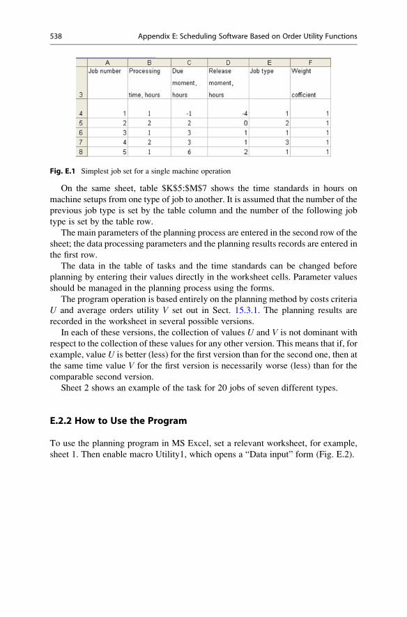
Fig. E.1 Simplest job set for a single machine operation
On the same sheet, table $K$5:$M$7 shows the time standards in hours on
machine setups from one type of job to another. It is assumed that the number of the
previous job type is set by the table column and the number of the following job
type is set by the table row.
The main parameters of the planning process are entered in the second row of the
sheet; the data processing parameters and the planning results records are entered in
the first row.
The data in the table of tasks and the time standards can be changed before
planning by entering their values directly in the worksheet cells. Parameter values
should be managed in the planning process using the forms.
The program operation is based entirely on the planning method by costs criteria
U and average orders utility V set out in Sect. 15.3.1. The planning results are
recorded in the worksheet in several possible versions.
In each of these versions, the collection of values U and V is not dominant with
respect to the collection of these values for any other version. This means that if, for
example, value U is better (less) for the first version than for the second one, then at
the same time value V for the first version is necessarily worse (less) than for the
comparable second version.
Sheet 2 shows an example of the task for 20 jobs of seven different types.
E.2.2 How to Use the Program
To use the planning program in MS Excel, set a relevant worksheet, for example,
sheet 1. Then enable macro Utility1, which opens a “Data input” form (Fig. E.2).
538 Appendix E: Scheduling Software Based on Order Utility Functions
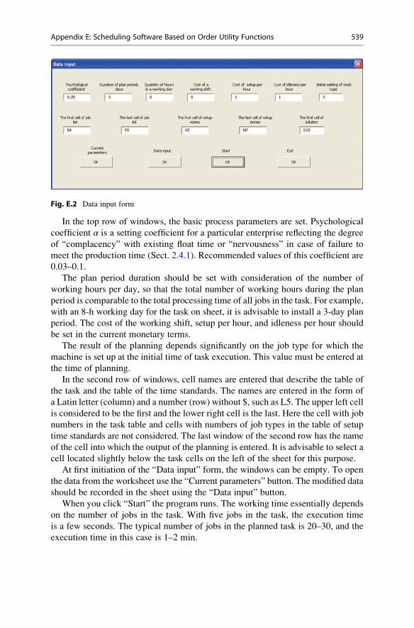
Fig. E.2 Data input form
In the top row of windows, the basic process parameters are set. Psychological
coefficient α is a setting coefficient for a particular enterprise reflecting the degree
of “complacency” with existing float time or “nervousness” in case of failure to
meet the production time (Sect. 2.4.1). Recommended values of this coefficient are
0.03–0.1.
The plan period duration should be set with consideration of the number of
working hours per day, so that the total number of working hours during the plan
period is comparable to the total processing time of all jobs in the task. For example,
with an 8-h working day for the task on sheet, it is advisable to install a 3-day plan
period. The cost of the working shift, setup per hour, and idleness per hour should
be set in the current monetary terms.
The result of the planning depends significantly on the job type for which the
machine is set up at the initial time of task execution. This value must be entered at
the time of planning.
In the second row of windows, cell names are entered that describe the table of
the task and the table of the time standards. The names are entered in the form of
a Latin letter (column) and a number (row) without $, such as L5. The upper left cell
is considered to be the first and the lower right cell is the last. Here the cell with job
numbers in the task table and cells with numbers of job types in the table of setup
time standards are not considered. The last window of the second row has the name
of the cell into which the output of the planning is entered. It is advisable to select a
cell located slightly below the task cells on the left of the sheet for this purpose.
At first initiation of the “Data input” form, the windows can be empty. To open
the data from the worksheet use the “Current parameters” button. The modified data
should be recorded in the sheet using the “Data input” button.
When you click “Start” the program runs. The working time essentially depends
on the number of jobs in the task. With five jobs in the task, the execution time
is a few seconds. The typical number of jobs in the planned task is 20–30, and the
execution time in this case is 1–2 min.
Appendix E: Scheduling Software Based on Order Utility Functions 539
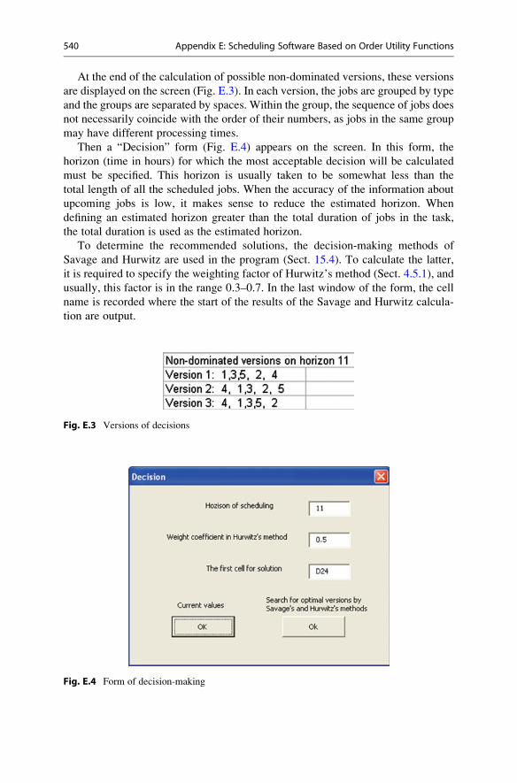
At the end of the calculation of possible non-dominated versions, these versions
are displayed on the screen (Fig. E.3). In each version, the jobs are grouped by type
and the groups are separated by spaces. Within the group, the sequence of jobs does
not necessarily coincide with the order of their numbers, as jobs in the same group
may have different processing times.
Then a “Decision” form (Fig. E.4) appears on the screen. In this form, the
horizon (time in hours) for which the most acceptable decision will be calculated
must be specified. This horizon is usually taken to be somewhat less than the
total length of all the scheduled jobs. When the accuracy of the information about
upcoming jobs is low, it makes sense to reduce the estimated horizon. When
defining an estimated horizon greater than the total duration of jobs in the task,
the total duration is used as the estimated horizon.
To determine the recommended solutions, the decision-making methods of
Savage and Hurwitz are used in the program (Sect. 15.4). To calculate the latter,
it is required to specify the weighting factor of Hurwitz’s method (Sect. 4.5.1), and
usually, this factor is in the range 0.3–0.7. In the last window of the form, the cell
name is recorded where the start of the results of the Savage and Hurwitz calcula-
tion are output.
Fig. E.3 Versions of decisions
Fig. E.4 Form of decision-making
540 Appendix E: Scheduling Software Based on Order Utility Functions
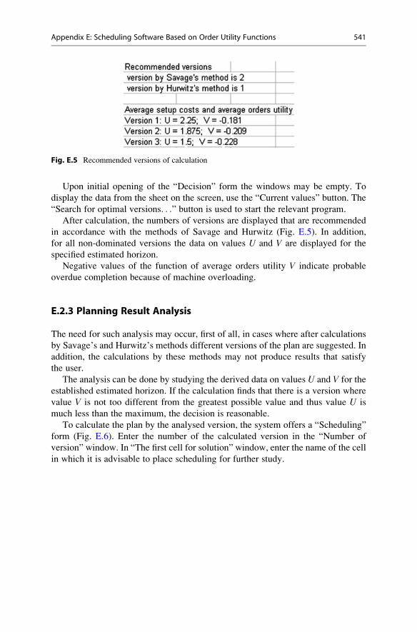
Upon initial opening of the “Decision” form the windows may be empty. To
display the data from the sheet on the screen, use the “Current values” button. The
“Search for optimal versions. . .” button is used to start the relevant program.
After calculation, the numbers of versions are displayed that are recommended
in accordance with the methods of Savage and Hurwitz (Fig. E.5). In addition,
for all non-dominated versions the data on values U and V are displayed for the
specified estimated horizon.
Negative values of the function of average orders utility V indicate probable
overdue completion because of machine overloading.
E.2.3 Planning Result Analysis
The need for such analysis may occur, first of all, in cases where after calculations
by Savage’s and Hurwitz’s methods different versions of the plan are suggested. In
addition, the calculations by these methods may not produce results that satisfy
the user.
The analysis can be done by studying the derived data on values U and V for the
established estimated horizon. If the calculation finds that there is a version where
value V is not too different from the greatest possible value and thus value U is
much less than the maximum, the decision is reasonable.
To calculate the plan by the analysed version, the system offers a “Scheduling”
form (Fig. E.6). Enter the number of the calculated version in the “Number of
version” window. In “The first cell for solution” window, enter the name of the cell
in which it is advisable to place scheduling for further study.
Fig. E.5 Recommended versions of calculation
Appendix E: Scheduling Software Based on Order Utility Functions 541
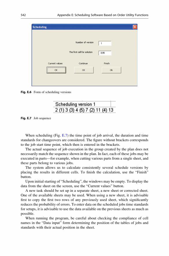
Fig. E.6 Form of scheduling versions
When scheduling (Fig. E.7) the time point of job arrival, the duration and time
standards for changeovers are considered. The figure without brackets corresponds
to the job start time point, which then is entered in the brackets.
The actual sequence of job execution in the group created by the plan does not
necessarily match the sequence shown in the plan. In fact, each of these jobs may be
executed in parts—for example, when cutting various parts from a single sheet, and
these parts belong to various jobs.
The system allows us to calculate consistently several schedule versions by
placing the results in different cells. To finish the calculation, use the “Finish”
button.
Upon initial starting of “Scheduling”, the windows may be empty. To display the
data from the sheet on the screen, use the “Current values” button.
A new task should be set up in a separate sheet, a new sheet or corrected sheet.
One of the available sheets may be used. When using a new sheet, it is advisable
first to copy the first two rows of any previously used sheet, which significantly
reduces the probability of errors. To enter data on the scheduled jobs time standards
for setups, it is advisable to use the data available on the previous sheets as much as
possible.
When running the program, be careful about checking the compliance of cell
names in the “Data input” form determining the position of the tables of jobs and
standards with their actual position in the sheet.
Fig. E.7 Job sequence
542 Appendix E: Scheduling Software Based on Order Utility Functions
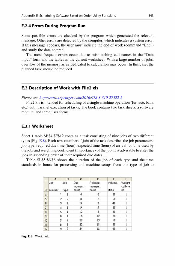
E.2.4 Errors During Program Run
Some possible errors are checked by the program which generated the relevant
message. Other errors are detected by the compiler, which indicates a system error.
If this message appears, the user must indicate the end of work (command “End”)
and study the data entered.
The most frequent errors occur due to mismatching cell names in the “Data
input” form and the tables in the current worksheet. With a large number of jobs,
overflow of the memory array dedicated to calculation may occur. In this case, the
planned task should be reduced.
E.3 Description of Work with File2.xls
Please see http://extras.springer.com/2016/978-3-319-27522-2File2.xls is intended for scheduling of a single-machine operation (furnace, bath,
etc.) with parallel execution of tasks. The book contains two task sheets, a software
module, and three user forms.
E.3.1 Worksheet
Sheet 1 table $B$4:$F$12 contains a task consisting of nine jobs of two different
types (Fig. E.8). Each row (number of job) of the task describes the job parameters:
job type, required due time (hour), expected time (hour) of arrival, volume used by
the job, and weighting coefficient (importance) of the job. It is advisable to enter the
jobs in ascending order of their required due dates.
Table $L$5:$N$6 shows the duration of the job of each type and the time
standards in hours for processing and machine setups from one type of job to
Fig. E.8 Work task
Appendix E: Scheduling Software Based on Order Utility Functions 543
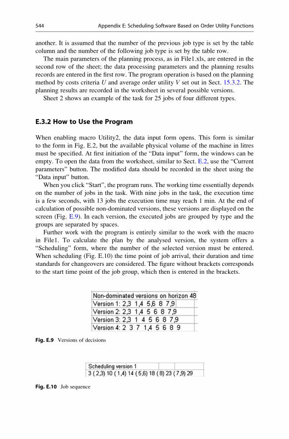
another. It is assumed that the number of the previous job type is set by the table
column and the number of the following job type is set by the table row.
The main parameters of the planning process, as in File1.xls, are entered in the
second row of the sheet; the data processing parameters and the planning results
records are entered in the first row. The program operation is based on the planning
method by costs criteria U and average order utility V set out in Sect. 15.3.2. The
planning results are recorded in the worksheet in several possible versions.
Sheet 2 shows an example of the task for 25 jobs of four different types.
E.3.2 How to Use the Program
When enabling macro Utility2, the data input form opens. This form is similar
to the form in Fig. E.2, but the available physical volume of the machine in litres
must be specified. At first initiation of the “Data input” form, the windows can be
empty. To open the data from the worksheet, similar to Sect. E.2, use the “Current
parameters” button. The modified data should be recorded in the sheet using the
“Data input” button.
When you click “Start”, the program runs. The working time essentially depends
on the number of jobs in the task. With nine jobs in the task, the execution time
is a few seconds, with 13 jobs the execution time may reach 1 min. At the end of
calculation of possible non-dominated versions, these versions are displayed on the
screen (Fig. E.9). In each version, the executed jobs are grouped by type and the
groups are separated by spaces.
Further work with the program is entirely similar to the work with the macro
in File1. To calculate the plan by the analysed version, the system offers a
“Scheduling” form, where the number of the selected version must be entered.
When scheduling (Fig. E.10) the time point of job arrival, their duration and time
standards for changeovers are considered. The figure without brackets corresponds
to the start time point of the job group, which then is entered in the brackets.
Fig. E.10 Job sequence
Fig. E.9 Versions of decisions
544 Appendix E: Scheduling Software Based on Order Utility Functions

E.4 Description of Work with File3.xls
Please see http://extras.springer.com/2016/978-3-319-27522-2File3.xls is intended for scheduling the operation of a production site consisting
of several parallel machines of the same purpose and using a “make-to-order”
strategy. The book contains two task sheets, a software module, and four user forms.
E.4.1 Worksheet
Sheet 1 table $A$5:$L$64 contains a task consisting of 60 jobs of six different types
(Fig. E.11). Each row of the task describes the job parameters: job number, required
due calendar day after start of schedule execution, expected calendar day of arrival
after start, job type, weighting coefficient (importance) of the job, and processing
time in hours on each machine. It is advisable to enter the jobs in ascending order of
their required due time points.
The main parameters of the planning process are entered in the second row of the
sheet; the data processing parameters and the planning results records are entered in
the first row.
Table $R$6:$BA$11 shows the time standards in hours for machine setups from
one type of job to another. It is assumed that the number of the previous job type is
set by the table column and the number of the following job type is set by the table
row. Region $S$13:$X$19 contains data on the machine condition at the start
of planning: cost of machine operation per hour, cost of idleness per hour, mark
of machine activation, and setup for the job type. Region $S$21:$AC$23 shows
the working calendar for 11 days starting from the first day of planning. For the
working day and machine utilization records, values 1 or 0 are used, and the
operation value is 1.
The program operation, as in the previous paragraphs, is based on the planning
method by costs criteria U and average order fulfilment utility V. The planning
results are recorded in the worksheet in several possible versions.
Fig. E.11 Work task fragment
Appendix E: Scheduling Software Based on Order Utility Functions 545
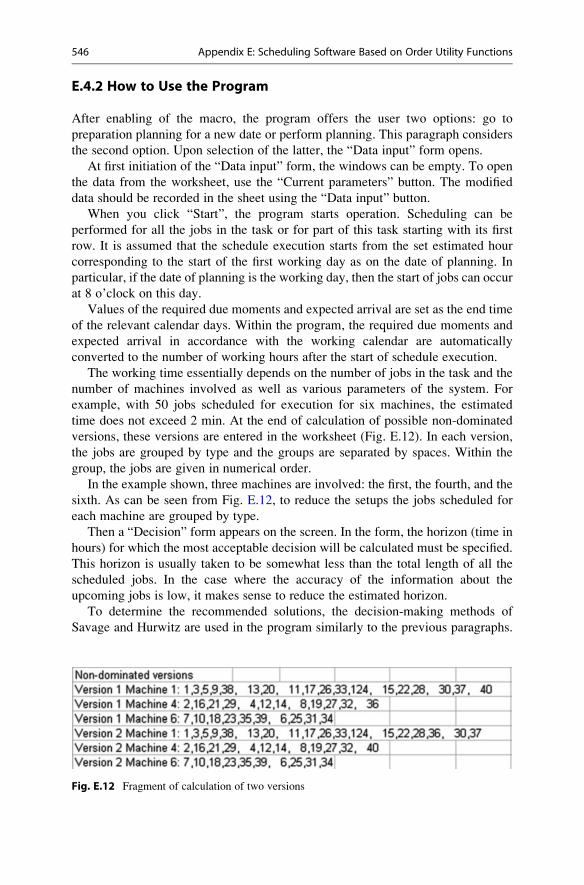
E.4.2 How to Use the Program
After enabling of the macro, the program offers the user two options: go to
preparation planning for a new date or perform planning. This paragraph considers
the second option. Upon selection of the latter, the “Data input” form opens.
At first initiation of the “Data input” form, the windows can be empty. To open
the data from the worksheet, use the “Current parameters” button. The modified
data should be recorded in the sheet using the “Data input” button.
When you click “Start”, the program starts operation. Scheduling can be
performed for all the jobs in the task or for part of this task starting with its first
row. It is assumed that the schedule execution starts from the set estimated hour
corresponding to the start of the first working day as on the date of planning. In
particular, if the date of planning is the working day, then the start of jobs can occur
at 8 o’clock on this day.
Values of the required due moments and expected arrival are set as the end time
of the relevant calendar days. Within the program, the required due moments and
expected arrival in accordance with the working calendar are automatically
converted to the number of working hours after the start of schedule execution.
The working time essentially depends on the number of jobs in the task and the
number of machines involved as well as various parameters of the system. For
example, with 50 jobs scheduled for execution for six machines, the estimated
time does not exceed 2 min. At the end of calculation of possible non-dominated
versions, these versions are entered in the worksheet (Fig. E.12). In each version,
the jobs are grouped by type and the groups are separated by spaces. Within the
group, the jobs are given in numerical order.
In the example shown, three machines are involved: the first, the fourth, and the
sixth. As can be seen from Fig. E.12, to reduce the setups the jobs scheduled for
each machine are grouped by type.
Then a “Decision” form appears on the screen. In the form, the horizon (time in
hours) for which the most acceptable decision will be calculated must be specified.
This horizon is usually taken to be somewhat less than the total length of all the
scheduled jobs. In the case where the accuracy of the information about the
upcoming jobs is low, it makes sense to reduce the estimated horizon.
To determine the recommended solutions, the decision-making methods of
Savage and Hurwitz are used in the program similarly to the previous paragraphs.
Fig. E.12 Fragment of calculation of two versions
546 Appendix E: Scheduling Software Based on Order Utility Functions

At the end of the calculation, a set of possible versions of the plan can be derived in
one of two ways. In the first case, all sustainable versions are derived from the
version with the greatest utility to the version recommended by the methods of
Savage or Hurwitz. In the second case, we can derive a minimum set of versions
between the version with the greatest utility and the version of the least duration.
Usually, it is recommended to use the first version.
For all non-dominated versions, the data on values U and V are displayed for the
specified estimated horizon. Also, the value of the load coefficient and the number
of the version with the least duration of total fulfilment of the task are recorded.
E.4.3 Planning Results Analysis
To calculate the plan by the analysed version, the system offers a “Scheduling”
form. Enter the number of the calculated version in the “Number of version”
window. The version with the least duration is used as the recommended one. In
“The first cell for solution” window, the name of the cell is entered in which it is
advisable to place scheduling for further study. When scheduling the time point of
job arrival, their duration and time standards for changeovers are considered
(Fig. E.13). The figure without brackets corresponds to the job start time point,
which then is entered in the brackets.
The quality of scheduling for parallel machines is significantly defined by the
uniformity of loading of all active machines. To evaluate this, at the end of the
schedule row for each machine the end time point of task execution is specified.
E.4.4 New Task
A new task is set up in a separate sheet, using a new sheet or a corrected sheet. One
of the available sheets may be used. It makes sense to copy the sheet with the last
plan task, rename this worksheet by the number in the file, and delete the planning
results belonging to the previous task from it.
In preparation for the new plan, put the completion mark (number 1) in the rows
of the last task. In the region describing the state of the machines, specify the date
for which the new plan is performed and put the marks of machines activation. Then
indicate the job type for which each machine will be set up by the beginning of the
Fig. E.13 Job sequence on parallel machines
Appendix E: Scheduling Software Based on Order Utility Functions 547
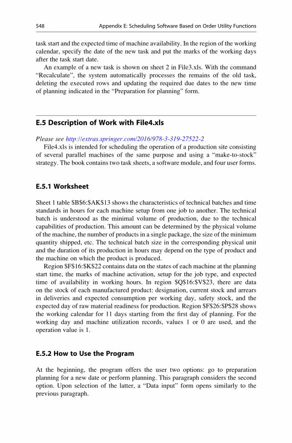
task start and the expected time of machine availability. In the region of the working
calendar, specify the date of the new task and put the marks of the working days
after the task start date.
An example of a new task is shown on sheet 2 in File3.xls. With the command
“Recalculate”, the system automatically processes the remains of the old task,
deleting the executed rows and updating the required due dates to the new time
of planning indicated in the “Preparation for planning” form.
E.5 Description of Work with File4.xls
Please see http://extras.springer.com/2016/978-3-319-27522-2File4.xls is intended for scheduling the operation of a production site consisting
of several parallel machines of the same purpose and using a “make-to-stock”
strategy. The book contains two task sheets, a software module, and four user forms.
E.5.1 Worksheet
Sheet 1 table $B$6:$AK$13 shows the characteristics of technical batches and time
standards in hours for each machine setup from one job to another. The technical
batch is understood as the minimal volume of production, due to the technical
capabilities of production. This amount can be determined by the physical volume
of the machine, the number of products in a single package, the size of the minimum
quantity shipped, etc. The technical batch size in the corresponding physical unit
and the duration of its production in hours may depend on the type of product and
the machine on which the product is produced.
Region $F$16:$K$22 contains data on the states of each machine at the planning
start time, the marks of machine activation, setup for the job type, and expected
time of availability in working hours. In region $Q$16:$V$23, there are data
on the stock of each manufactured product: designation, current stock and arrears
in deliveries and expected consumption per working day, safety stock, and the
expected day of raw material readiness for production. Region $F$26:$P$28 shows
the working calendar for 11 days starting from the first day of planning. For the
working day and machine utilization records, values 1 or 0 are used, and the
operation value is 1.
E.5.2 How to Use the Program
At the beginning, the program offers the user two options: go to preparation
planning for a new date or perform planning. This paragraph considers the second
option. Upon selection of the latter, a “Data input” form opens similarly to the
previous paragraph.
548 Appendix E: Scheduling Software Based on Order Utility Functions
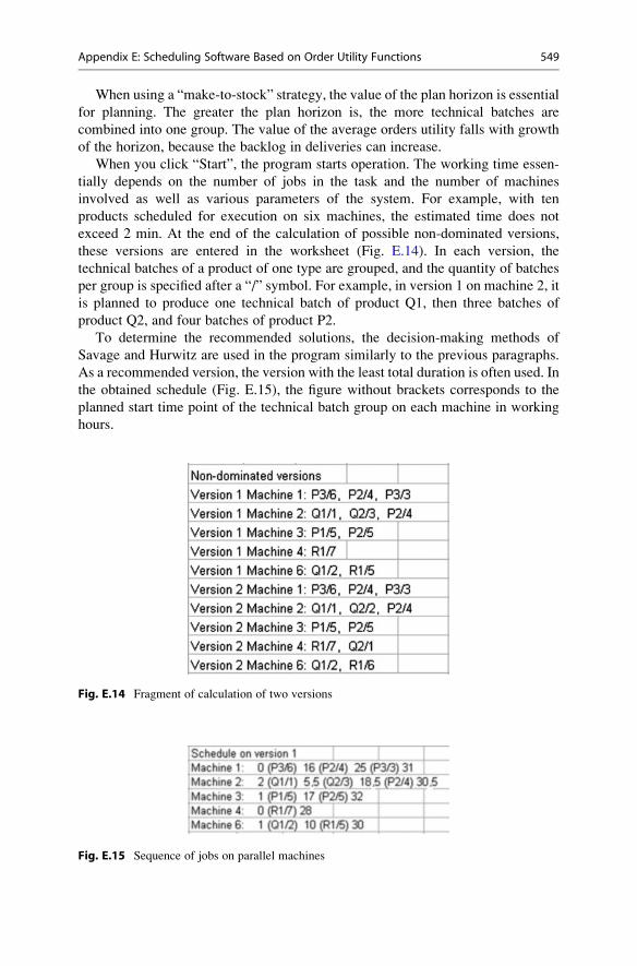
When using a “make-to-stock” strategy, the value of the plan horizon is essential
for planning. The greater the plan horizon is, the more technical batches are
combined into one group. The value of the average orders utility falls with growth
of the horizon, because the backlog in deliveries can increase.
When you click “Start”, the program starts operation. The working time essen-
tially depends on the number of jobs in the task and the number of machines
involved as well as various parameters of the system. For example, with ten
products scheduled for execution on six machines, the estimated time does not
exceed 2 min. At the end of the calculation of possible non-dominated versions,
these versions are entered in the worksheet (Fig. E.14). In each version, the
technical batches of a product of one type are grouped, and the quantity of batches
per group is specified after a “/” symbol. For example, in version 1 on machine 2, it
is planned to produce one technical batch of product Q1, then three batches of
product Q2, and four batches of product P2.
To determine the recommended solutions, the decision-making methods of
Savage and Hurwitz are used in the program similarly to the previous paragraphs.
As a recommended version, the version with the least total duration is often used. In
the obtained schedule (Fig. E.15), the figure without brackets corresponds to the
planned start time point of the technical batch group on each machine in working
hours.
Fig. E.15 Sequence of jobs on parallel machines
Fig. E.14 Fragment of calculation of two versions
Appendix E: Scheduling Software Based on Order Utility Functions 549

The schedule quality for parallel machines is significantly determined by
uniform loading of all machines. For this assessment at the end of the schedule
row for each machine, the end time point of the task is specified.
Below the schedule, the total calculation of stock dynamics for each product is
presented for the selected schedule version (Fig. E.16). The figure without brackets,
as above, corresponds to the release time point of the new batch of product in
working hours.
In brackets, in general, three numbers separated by “/” symbols are given. The
first number indicates the amount of stock in thousands of litres by the time of new
receipt; the second number corresponds to the stock after delivery; the third number
reflects the backlog in delivery at the time of product receipt. If the debt is zero, then
it is not given in the text.
In preparation for the new plan, in the region describing the state of the machines
specify the date for which new planning is performed and put the marks of machine
activation. Then indicate the job type for which each machine will be set up by the
beginning of the task start and the expected time of machine release. In the region
of the working calendar, specify the date of the task start and put marks of the
working days after the date of task start. In the region of the stock, correct the values
of the available stock, backlog in deliveries, and terms of raw material receipt. An
example of a new task is shown in sheet 2 in File4.xls.
E.6 Description of Work with File5.xls
Please see http://extras.springer.com/2016/978-3-319-27522-2File5.xls is intended for scheduling the operation of a production site consisting
of machines of different purpose and using a “make-to-order” strategy. It is
assumed that the uniform machines have similar technological capabilities and
can be considered as one group of machines. The book contains two task sheets,
a software module, and four user forms.
Fig. E.16 Stock dynamics
550 Appendix E: Scheduling Software Based on Order Utility Functions
E.6.1 Worksheet
Sheet 1 table $A$5:$F$24 contains a task consisting of 20 jobs of six different
types. Each row (number of job) of the task describes the job parameters: job
number, required due calendar day after start of schedule execution, expected
calendar day of arrival after start, job type, weighting coefficient (importance) of
the job, and completion mark. The job type can mean a specific part or a group
of similar parts manufactured according to the same process using the same tools.
The sequence of operations of each process is fixed and is different for different
processes. It is advisable to enter the jobs in ascending order of their required due
time points.
Table $H$5:$L$84 is a list of operations for all the jobs in table $A$5:$F$24.
Each row of this table contains the number of the operation, group of machines
on which the operation must be performed, processing time in hours, and expected
end time point in hours after the start of schedule execution. The operations of each
job should be sorted in the order of their execution. If the value of the expected due
time point equals 0, this means the relevant operation is already executed. For an
operation that has not yet commenced, the expected due time point is 1.
Table $O$17:$S$22 shows time standards in hours for setup of each machine
from one type of job to another. Table $O$5:$Q$9 presents the characteristics of
the machine groups in the production area: quantity of machines in the group, cost
of setup per hour, and cost of idleness per hour.
Region $U$5:$Y$12 contains data on each machine condition at the time of
planning start: inventory number of the machine; group number, which the machine
refers to; mark of machine activation; setup for the job type; and expected moment
of release in hours after the start of schedule execution. Region $Q$21:$S$27
shows the working calendar for 10 days starting from the first day of planning.
For the working day and machine utilization records, values 1 or 0 are used, and the
operation value is 1.
E.6.2 How to Use the Program
At the beginning, the program offers the user two options: go to preparation planning
for a new date or perform planning. This paragraph considers the second option.
Upon selection of the latter, a “Data input” form opens similarly to the previous
paragraphs.
When you click “Start”, the program starts operation. It is assumed that the
schedule execution starts from the set estimated hour corresponding to the start of
the first working day as on the date of planning. In particular, if the date of planning
is the working day, then the start of jobs can occur at 8 o’clock on this day. Values of
the required due moments and expected arrival are set as the end time of the relevant
calendar days. Within the program, the required due moments and expected arrival
in accordance with the working calendar are automatically converted to the number
of working hours after the start of schedule execution.
Appendix E: Scheduling Software Based on Order Utility Functions 551
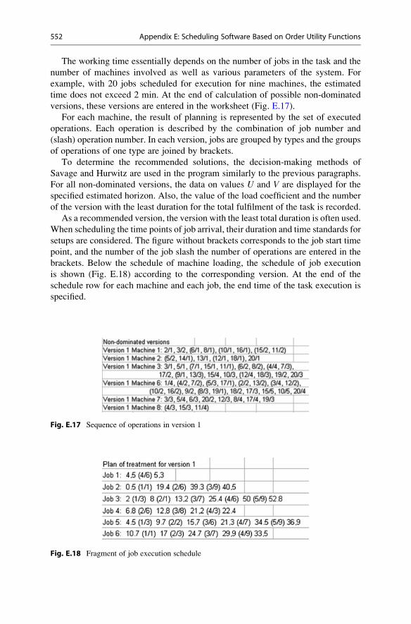
The working time essentially depends on the number of jobs in the task and the
number of machines involved as well as various parameters of the system. For
example, with 20 jobs scheduled for execution for nine machines, the estimated
time does not exceed 2 min. At the end of calculation of possible non-dominated
versions, these versions are entered in the worksheet (Fig. E.17).
For each machine, the result of planning is represented by the set of executed
operations. Each operation is described by the combination of job number and
(slash) operation number. In each version, jobs are grouped by types and the groups
of operations of one type are joined by brackets.
To determine the recommended solutions, the decision-making methods of
Savage and Hurwitz are used in the program similarly to the previous paragraphs.
For all non-dominated versions, the data on values U and V are displayed for the
specified estimated horizon. Also, the value of the load coefficient and the number
of the version with the least duration for the total fulfilment of the task is recorded.
As a recommended version, the version with the least total duration is often used.
When scheduling the time points of job arrival, their duration and time standards for
setups are considered. The figure without brackets corresponds to the job start time
point, and the number of the job slash the number of operations are entered in the
brackets. Below the schedule of machine loading, the schedule of job execution
is shown (Fig. E.18) according to the corresponding version. At the end of the
schedule row for each machine and each job, the end time of the task execution is
specified.
Fig. E.18 Fragment of job execution schedule
Fig. E.17 Sequence of operations in version 1
552 Appendix E: Scheduling Software Based on Order Utility Functions
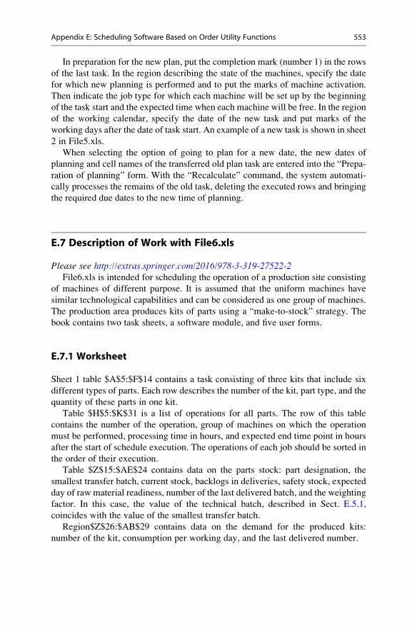
In preparation for the new plan, put the completion mark (number 1) in the rows
of the last task. In the region describing the state of the machines, specify the date
for which new planning is performed and to put the marks of machine activation.
Then indicate the job type for which each machine will be set up by the beginning
of the task start and the expected time when each machine will be free. In the region
of the working calendar, specify the date of the new task and put marks of the
working days after the date of task start. An example of a new task is shown in sheet
2 in File5.xls.
When selecting the option of going to plan for a new date, the new dates of
planning and cell names of the transferred old plan task are entered into the “Prepa-
ration of planning” form. With the “Recalculate” command, the system automati-
cally processes the remains of the old task, deleting the executed rows and bringing
the required due dates to the new time of planning.
E.7 Description of Work with File6.xls
Please see http://extras.springer.com/2016/978-3-319-27522-2File6.xls is intended for scheduling the operation of a production site consisting
of machines of different purpose. It is assumed that the uniform machines have
similar technological capabilities and can be considered as one group of machines.
The production area produces kits of parts using a “make-to-stock” strategy. The
book contains two task sheets, a software module, and five user forms.
E.7.1 Worksheet
Sheet 1 table $A$5:$F$14 contains a task consisting of three kits that include six
different types of parts. Each row describes the number of the kit, part type, and the
quantity of these parts in one kit.
Table $H$5:$K$31 is a list of operations for all parts. The row of this table
contains the number of the operation, group of machines on which the operation
must be performed, processing time in hours, and expected end time point in hours
after the start of schedule execution. The operations of each job should be sorted in
the order of their execution.
Table $Z$15:$AE$24 contains data on the parts stock: part designation, the
smallest transfer batch, current stock, backlogs in deliveries, safety stock, expected
day of raw material readiness, number of the last delivered batch, and the weighting
factor. In this case, the value of the technical batch, described in Sect. E.5.1,
coincides with the value of the smallest transfer batch.
Region$Z$26:$AB$29 contains data on the demand for the produced kits:
number of the kit, consumption per working day, and the last delivered number.
Appendix E: Scheduling Software Based on Order Utility Functions 553

Table $Z$31:$ADE$36 has data on the condition of the parts batch in process:
part number, batch number, quantity in a batch, last performed (fulfilled) operation,
and the expected due time point in hours.
The data on the machine condition, time standards, and working calendar are
entered in the worksheet similarly to the previous program.
E.7.2 How to Use the Program
At the beginning, the program offers the user two options: go to preparation
planning for a new date or perform planning. This paragraph considers the second
option, which in turn offers two actions: initial calculation and simulation.
If simulation is not performed (initial calculation mode), then a “Data input”
form opens. It enables inputting of necessary tables.
When you click “Start”, the program starts operation, and the calculation result
is entered in the sheet (Fig. E.19).
For each machine, the scheduling result is a set of operations. Each operation is
described by a combination of the part number, (with slash sign) quantity of transfer
batch, and (with slash sign) operation number. In each version, several transfer
batches (in parentheses) are automatically combined into one technological batch.
For example, on machine 1 for part 3 transfer batches 19, 20, 21, and 22 are
combined into a single group to perform operation 1.
The relevant schedule of machine load is presented in Fig. E.20. For each
machine, the sequence of start time points is recorded. After each time point is a
combination of the part number, (with slash sign) operation number, and (with slash
sign) the quantity of parts in a technological batch.
Fig. E.19 Sequence of operations in version 1
554 Appendix E: Scheduling Software Based on Order Utility Functions
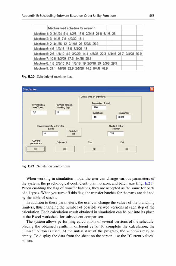
Fig. E.20 Schedule of machine load
When working in simulation mode, the user can change various parameters of
the system: the psychological coefficient, plan horizon, and batch size (Fig. E.21).
When enabling the flag of transfer batches, they are accepted as the same for parts
of all types. When you turn off this flag, the transfer batches for the parts are defined
by the table of stocks.
In addition to these parameters, the user can change the values of the branching
limiters, thus changing the number of possible viewed versions at each step of the
calculation. Each calculation result obtained in simulation can be put into its place
in the Excel worksheet for subsequent comparison.
The system allows performing calculations of several versions of the schedule,
placing the obtained results in different cells. To complete the calculation, the
“Finish” button is used. At the initial start of the program, the windows may be
empty. To display the data from the sheet on the screen, use the “Current values”
button.
Fig. E.21 Simulation control form
Appendix E: Scheduling Software Based on Order Utility Functions 555
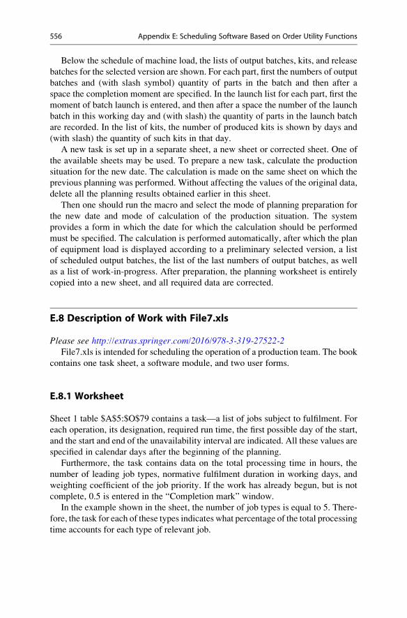
Below the schedule of machine load, the lists of output batches, kits, and release
batches for the selected version are shown. For each part, first the numbers of output
batches and (with slash symbol) quantity of parts in the batch and then after a
space the completion moment are specified. In the launch list for each part, first the
moment of batch launch is entered, and then after a space the number of the launch
batch in this working day and (with slash) the quantity of parts in the launch batch
are recorded. In the list of kits, the number of produced kits is shown by days and
(with slash) the quantity of such kits in that day.
A new task is set up in a separate sheet, a new sheet or corrected sheet. One of
the available sheets may be used. To prepare a new task, calculate the production
situation for the new date. The calculation is made on the same sheet on which the
previous planning was performed. Without affecting the values of the original data,
delete all the planning results obtained earlier in this sheet.
Then one should run the macro and select the mode of planning preparation for
the new date and mode of calculation of the production situation. The system
provides a form in which the date for which the calculation should be performed
must be specified. The calculation is performed automatically, after which the plan
of equipment load is displayed according to a preliminary selected version, a list
of scheduled output batches, the list of the last numbers of output batches, as well
as a list of work-in-progress. After preparation, the planning worksheet is entirely
copied into a new sheet, and all required data are corrected.
E.8 Description of Work with File7.xls
Please see http://extras.springer.com/2016/978-3-319-27522-2File7.xls is intended for scheduling the operation of a production team. The book
contains one task sheet, a software module, and two user forms.
E.8.1 Worksheet
Sheet 1 table $A$5:$O$79 contains a task—a list of jobs subject to fulfilment. For
each operation, its designation, required run time, the first possible day of the start,
and the start and end of the unavailability interval are indicated. All these values are
specified in calendar days after the beginning of the planning.
Furthermore, the task contains data on the total processing time in hours, the
number of leading job types, normative fulfilment duration in working days, and
weighting coefficient of the job priority. If the work has already begun, but is not
complete, 0.5 is entered in the “Completion mark” window.
In the example shown in the sheet, the number of job types is equal to 5. There-
fore, the task for each of these types indicates what percentage of the total processing
time accounts for each type of relevant job.
556 Appendix E: Scheduling Software Based on Order Utility Functions

Table $S$6:$W$10 contains the largest possible output per hour/day for each
type of job for the relevant team. Table $S$20:$Y$35 indicates the percentage of
completion of five started jobs for each job type as of 01.04.14. Region $S$64:$
AD$75 in the working calendar as of 01.04.14 contains the tentative interests of
planned performance for all types of jobs for the next 10 weeks.
E.8.2 How to Use the Program
When you click “Start”, the program starts operation. The result of the calculation is
an execution schedule of jobs, in which for each job the calendar start and end dates
are indicated. In parentheses, the numbers of production teams performing these
jobs are recorded, and the first team is the team that performs the leading type
of jobs.
In addition to the schedule, the program displays three tables of team load in the
worksheet. In the top table (Fig. E.22), the weekly load factor of each team as a
percentage of the maximum possible performance is recorded. The middle table
shows the list of jobs executed by the team during each week. The lower table
shows weekly team load for each job type in hours.
The schedule of jobs prepared automatically is the first approximation to the
optimal one and can be improved. Correction of schedules is performed using a
“Correction” form. In the form, it is possible to set the values of the end time points
of jobs and the duration of five jobs. When the program is in “Correction” mode, the
system automatically takes into account the specified changes and moves the start
and end points of jobs to more appropriate times. With enough skills in simulation,
it is possible to achieve significant improvement in schedules for both timely
execution of jobs and more uniform utilization of production teams.
E.9 Description of Work with File8.xls
Please see http://extras.springer.com/2016/978-3-319-27522-2File8.xls is intended for scheduling the operation of a production site consisting
of machines of different purposes and using a “make-to-order” strategy. Compared
Fig. E.22 Weekly team load
Appendix E: Scheduling Software Based on Order Utility Functions 557
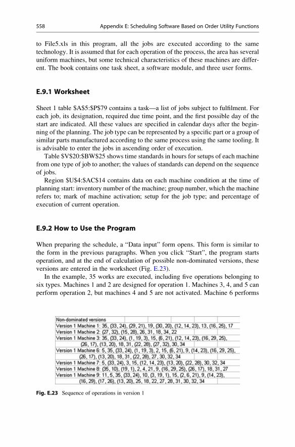
to File5.xls in this program, all the jobs are executed according to the same
technology. It is assumed that for each operation of the process, the area has several
uniform machines, but some technical characteristics of these machines are differ-
ent. The book contains one task sheet, a software module, and three user forms.
E.9.1 Worksheet
Sheet 1 table $A$5:$P$79 contains a task—a list of jobs subject to fulfilment. For
each job, its designation, required due time point, and the first possible day of the
start are indicated. All these values are specified in calendar days after the begin-
ning of the planning. The job type can be represented by a specific part or a group of
similar parts manufactured according to the same process using the same tooling. It
is advisable to enter the jobs in ascending order of execution.
Table $V$20:$BW$25 shows time standards in hours for setups of each machine
from one type of job to another; the values of standards can depend on the sequence
of jobs.
Region $U$4:$AC$14 contains data on each machine condition at the time of
planning start: inventory number of the machine; group number, which the machine
refers to; mark of machine activation; setup for the job type; and percentage of
execution of current operation.
E.9.2 How to Use the Program
When preparing the schedule, a “Data input” form opens. This form is similar to
the form in the previous paragraphs. When you click “Start”, the program starts
operation, and at the end of calculation of possible non-dominated versions, these
versions are entered in the worksheet (Fig. E.23).
In the example, 35 works are executed, including five operations belonging to
six types. Machines 1 and 2 are designed for operation 1. Machines 3, 4, and 5 can
perform operation 2, but machines 4 and 5 are not activated. Machine 6 performs
Fig. E.23 Sequence of operations in version 1
558 Appendix E: Scheduling Software Based on Order Utility Functions

operation 3, machines 7 and 8 are intended for operation 4, and machine 9 is
necessary for operation 5.
As can be seen from the example, in the resulting schedule the jobs are grouped
by type. The machine group load for each operation is in the range 0.82–1.19. The
density of the load of the machines varies. The greatest density (86 %) is observed
on machine 3 and the least (28 %) is observed on machine 7.
Appendix E: Scheduling Software Based on Order Utility Functions 559

Appendix F: Using Clobbi1
F.1 General
This appendix gives a short description of the basic production planning capabilities
in Clobbi SaaS manufacturing management system (http://clobbi.com), built on
contemporary cloud technologies.
The Clobbi service is based on the IT-Enterprise ERP system (www.it.ua, www.it-
enterprise.ru) platform, widely used in industrial enterprises in Eastern European
countries, which includes ready solutions for automation of all services of an indus-
trial enterprise in manufacturing and resource management (MRP II, MES, APS),
sales management, supply chain management (SCM), procurement management,
equipment operation and maintenance management (EAM), quality management,
human resources and payroll (HR), finance planning and budgeting, accounting, and
tax. Clobbi uses trusted typical solutions and the best business practice accumulating
more than 20 years’ experience of IT-Enterprise in manufacturing management.
To start work with the service demo version, please go to http://clobbi.com/
demo and download the demo version after the registration procedure.
After client application deploys, you will find a “Clobbi” shortcut on your
desktop. When starting the shortcut, you should enter “PLAN” into the login and
password fields to view the system as Chief planner.
Go to the Clobbi main menu and desktop. On the right, you will see operating
instructions that will help you to learn about the system interface and understand its
functionality (Fig. F.1).
1 This material is provided by the IT-Enterprise Corporation.
# Springer International Publishing Switzerland 2016
Y. Mauergauz, Advanced Planning and Scheduling in Manufacturing and SupplyChains, DOI 10.1007/978-3-319-27523-9
561
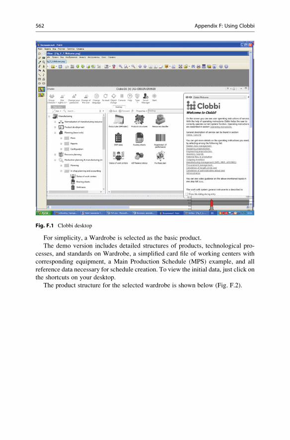
Fig. F.1 Clobbi desktop
For simplicity, a Wardrobe is selected as the basic product.
The demo version includes detailed structures of products, technological pro-
cesses, and standards on Wardrobe, a simplified card file of working centers with
corresponding equipment, a Main Production Schedule (MPS) example, and all
reference data necessary for schedule creation. To view the initial data, just click on
the shortcuts on your desktop.
The product structure for the selected wardrobe is shown below (Fig. F.2).
562 Appendix F: Using Clobbi
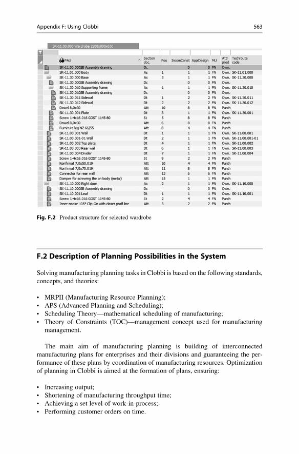
Fig. F.2 Product structure for selected wardrobe
F.2 Description of Planning Possibilities in the System
Solving manufacturing planning tasks in Clobbi is based on the following standards,
concepts, and theories:
• MRPII (Manufacturing Resource Planning);
• APS (Advanced Planning and Scheduling);
• Scheduling Theory—mathematical scheduling of manufacturing;
• Theory of Constraints (TOC)—management concept used for manufacturing
management.
The main aim of manufacturing planning is building of interconnected
manufacturing plans for enterprises and their divisions and guaranteeing the per-
formance of these plans by coordination of manufacturing resources. Optimization
of planning in Clobbi is aimed at the formation of plans, ensuring:
• Increasing output;
• Shortening of manufacturing throughput time;
• Achieving a set level of work-in-process;
• Performing customer orders on time.
Appendix F: Using Clobbi 563
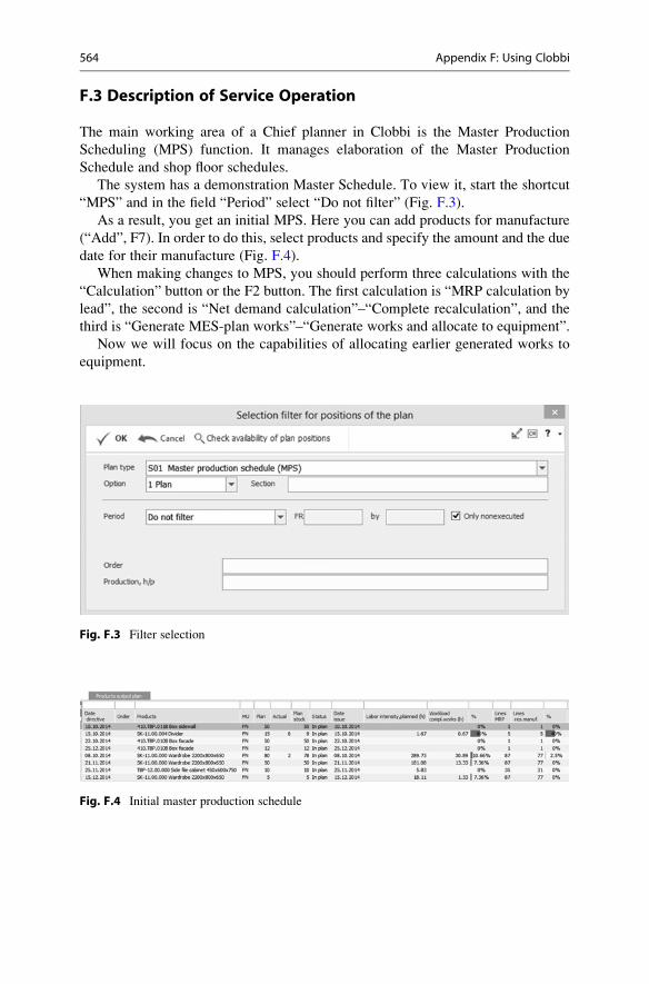
F.3 Description of Service Operation
The main working area of a Chief planner in Clobbi is the Master Production
Scheduling (MPS) function. It manages elaboration of the Master Production
Schedule and shop floor schedules.
The system has a demonstration Master Schedule. To view it, start the shortcut
“MPS” and in the field “Period” select “Do not filter” (Fig. F.3).
As a result, you get an initial MPS. Here you can add products for manufacture
(“Add”, F7). In order to do this, select products and specify the amount and the due
date for their manufacture (Fig. F.4).
When making changes to MPS, you should perform three calculations with the
“Calculation” button or the F2 button. The first calculation is “MRP calculation by
lead”, the second is “Net demand calculation”–“Complete recalculation”, and the
third is “Generate MES-plan works”–“Generate works and allocate to equipment”.
Now we will focus on the capabilities of allocating earlier generated works to
equipment.
Fig. F.3 Filter selection
Fig. F.4 Initial master production schedule
564 Appendix F: Using Clobbi

F.3.1 Generating Manufacturing Schedules
The task of operational calendar optimization manufacturing planning (APS/MES
planning) is the performance of MPS and/or MRP plans of manufacturing by the
optimal distribution of operations in time. As a result of optimization, manufacturing
orders are produced on time or with minimum violations, capacity utilization is
denser, the duration and numbers of equipment changeovers are decreased, idle
time and volumes of unfinished manufacturing are reduced, the total duration of the
manufacturing cycle is shortened, and, consequently, production output is increased
and material and financial resources turnover is accelerated.
An APS/MES plan is generated taking into account limited capacity utilization,
actual and forecast availability of materials, and other manufacturing resources. As
a result, we get detailed shift operational manufacturing plans for each working
center with optimal sequence of order performance.
APS/MES planning is the extension of usual calendar production planning with
limited capacity. The main differences are the following:
• Absence of calendar planning intervals;
• Location of all works on a time axis with the accuracy of minutes;
• As follows from the previous point, the possibility of accounting during planning
the actual sequence of works, setup time, time of waiting, and transfer between
working centers;
• The plan is generated according to one or several optimization criteria.
Let’s generate a manufacturing schedule based on the demonstration example.
To do this, while in MPS plan, we will use calculation F2 “Generation of MES-plan
works”–“Call interface of work appointment” (Fig. F.5).
After specifying the date-time of the start point, you will get more or less the
same picture of work appointment for the existing list of working centers. On the
left you will see the list of working centers with the indicators of load. In the
middle, a Gantt chart for visualization. If you point the cursor to any work, you will
get a detailed work description. On the right you will see a slider to control the
Fig. F.5 Selection of calculation
Appendix F: Using Clobbi 565
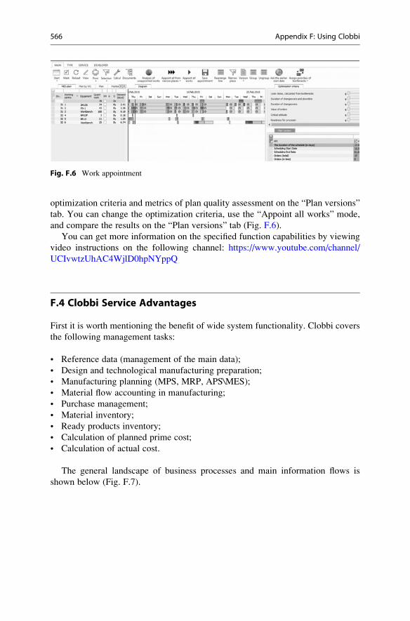
optimization criteria and metrics of plan quality assessment on the “Plan versions”
tab. You can change the optimization criteria, use the “Appoint all works” mode,
and compare the results on the “Plan versions” tab (Fig. F.6).
You can get more information on the specified function capabilities by viewing
video instructions on the following channel: https://www.youtube.com/channel/
UCIvwtzUhAC4WjlD0hpNYppQ
F.4 Clobbi Service Advantages
First it is worth mentioning the benefit of wide system functionality. Clobbi covers
the following management tasks:
• Reference data (management of the main data);
• Design and technological manufacturing preparation;
• Manufacturing planning (MPS, MRP, APS\MES);
• Material flow accounting in manufacturing;
• Purchase management;
• Material inventory;
• Ready products inventory;
• Calculation of planned prime cost;
• Calculation of actual cost.
The general landscape of business processes and main information flows is
shown below (Fig. F.7).
Fig. F.6 Work appointment
566 Appendix F: Using Clobbi

Fig. F.7 General system landscape
Why Clobbi is recommended solution:
• Pre-installed typical system functionality for manufacturing enterprise with a
discrete type of manufacture (machine and instrumentation building with multi-
ple sub-industries).
• Possibility of using the system as a complex solution for the management of
interconnected business processes as well as the combination of separate services
for the solution of specific tasks of manufacturing enterprise management.
• Hot deployment of the management system. The enterprise can start working
with the service in 1 day.
• Easy economic start of management in ERP. Minimization of initial investment,
as there is no need to buy high production expensive server equipment.
• Guaranteed service efficiency. Scheduled maintenance and technical support of
the system is provided by the solution developer. You can totally concentrate on
the everyday use and development of your business processes.
• Service scalability. The enterprise can extend the functionality of its manage-
ment system and you can buy additional competitive licenses if necessary.
• Availability of the management system. Clobbi provides access for users 24 h a
day, 7 days a week. Users can work online from any computer.
You can learn about the product from Clobbi Youtube channel on a separate
playlist https://www.youtube.com/channel/UCIvwtzUhAC4WjlD0hpNYppQ, where
you can find review materials and video instructions on all approaches mentioned
above. The same video instructions are available directly from Clobbi interface.
Appendix F: Using Clobbi 567
F.5 Online Registration of Manufacturing Events
For the full use of planning algorithms of levels MRP and APS\MES, you should
solve the tasks of material inventory, components, and unfinished manufacture in
manufacturing divisions. It is advisable to solve these tasks by using Clobbi.
The main goal of running operational inventory or material flows is to answer the
following questions:
• What production orders are currently started;
• What part operation is in progress now for each production order (PO);
• What is going on now in each working center:
– if debugging or processing is in progress—what part operation, what PO,
when it was started, and when it is scheduled for finish;
– if a working center is idle—what is the cause of idle time and how long it will
be;
• Where parts or assemblies for each production order are located;
• Where are defects detected, when and how many.
Clobbi uses a documentary approach tomanufacturing accounting, i.e. registering
information on the manufacturing process, the system automatically provides esti-
mation of material balance, parts, and assemblies in unfinished manufacturing,
accounting of different manufacturing events, and performance of manufacturing
plans.
The main manufacturing documents are:
• Manufacture act of part operations with recording lines of amortization;
• Waybill on parts and assemblies transfer;
• Documents of registration and repair of defects.
All actions on the manufacturing inventory can be performed traditionally on a
computer (desktop or laptop with MS Windows) and by means of entering infor-
mation from a mobile Android device.
The recommended option for the generation and processing of specified
documents is the registration of corresponding events with the help of the mobile
Android application Clobbi.Manufacture (to use in manufacturing divisions, you
should connect to Wi-Fi and install this application from PlayMarket).
Clobbi.Manufacture is intended for online receipt of manufacturing tasks and
registration of information on the manufacturing process in Clobbi. The application
opens new horizons for information selection and analysis. Users of the mobile
application Clobbi.Manufacture receive an easy at-hand tool that allows the
following:
• Receiving manufacturing tasks online;
• Receiving information on the status of manufacturing orders and tasks;
568 Appendix F: Using Clobbi

• Viewing technical documentation on parts, assemblies, and s/p frommanufacturing
tasks (drawings, technological processes, standards);
• Registering actual start and end of tasks online;
• Registering equipment idle time indicating the causes of idle time;
• Seeing event history by route lists;
• Tracking intrashop process of manufacturing parts, assemblies, and s/p.
The use of Clobbi.Manufacture considerably increases the mobility of employees
and the efficiency of their work (Fig. F.8).
The basis for the start of part manufacturing is the shift task sent to an employee.
The start and end of each operation must be recorded in Clobbi, using one of
several methods: manual recording on start/end in shift task or route list, using bar
coding, etc.
The registration of the end of operation is the input of the actual volume of
work—number of processed parts and assembly units (PAU), number of parts for
technological needs, and correctable and final defects.
Moreover, the transfer of parts and assemblies between working centers and
manufacturing divisions as well as idle time on working centers are registered.
F.6 Clobbi Commercial Use
The commercial version of Clobbi is based on the highly reliable worldwide cloud
service Windows Azure (http://azure.microsoft.com).
Fig. F.8 The user’s mobile application
Appendix F: Using Clobbi 569

To start the commercial use of the service, you should complete the registration
form on the website http://clobbi.com/buy/. You will then receive an e-mail from
the technical support service with a link for the system installation in “click
once” mode.
The installation process takes several minutes. After its completion, you will
have a shortcut to Clobbi on your desktop.
570 Appendix F: Using Clobbi