ADVANCED GEOMETRY-BASED MODELING FOR MIMO SCENARIOS IN COMPARISONWITH REAL MEASUREMENTS

Giovanni Del Galdo1, Jorg Lotze1, Martin Haardt1, and Christian Schneider2

Ilmenau University of Technology1. Communications Research Laboratory2. Measurements Engineering Laboratory

P.O. Box 100565D-98684 Ilmenau, Germany

ABSTRACT

The scenario encountered in a recent measurement cam-paign undertaken at Ilmenau University of Technology hasbeen artificially reconstructed in a computer-based prop-agation model for wireless communications developed bythe authors. The real measurements have been collectedwith the RUSK MIMO multidimensional channel sounder(Thoma et al., 2001). The program which implements themodel includes a geometrical representation of the environ-ment surrounding the experiment and a precise representa-tion of the transmitting and receiving antennas. The analysisof all this information leads to a synthetic data set similar tothe one actually measured. From the comparisons of thetwo channel matrices it is possible to derive useful infor-mation to improve the model itself and to better understandthe physical origins of small-scale fading. In particular theeffects of the different parameters on the synthetic chan-nel have been studied in order to assess the sensibility ofthe model. This analysis shows that the correct positioningof a small number of scatterers is enough to achieve fre-quency selectiveness as well as specific traits of the channelstatistics. The size of the scattering clusters, the number ofscatterers per cluster, and the Rician K-factor can be modi-fied in order to tune the channel statistics at will. To obtainhigher levels of time variance, moving scatterers or time de-pendent reflection coefficients must be introduced.

1. INTRODUCTION

The high complexity of the propagation phenomenon sets avast challenge in the effort of modeling the wireless chan-nel. The most accurate approach would be to solve theMaxwell equations. However the computational effort re-quired would be prohibitive, especially if we consideredmultiple antennas at both ends of the link, i.e., a MIMO sys-tem (Multiple Input Multiple Output). In fact, if MR andMT are the number of antennas at the receiver and at the

transmitter, respectively, the number of channels to be cal-culated grows to MR ·MT . Furthermore a precise physicaland geometrical description of the objects would be neces-sary.

In order to reduce the complexity of the model the socalled GTD (Geometric Theory of Diffraction) can be em-ployed (Correia, 2001). This approach postulates the exis-tence of direct, diffracted and reflected rays only. As thewavelength λ approaches zero, this approximation becomesincreasingly accurate.

With a ray-tracing engine and a full 3D description ofthe environment it is then possible to calculate all possi-ble rays linking the antennas. However with a GTD ap-proach a complete geometrical representation of the sce-nario is still required. A further approximation is to sim-plify the geometry surrounding the antennas with a discretenumber of reflectors, called scatterers; when only direct andreflected rays are considered the computational complexitydrops significantly. In this paper we present a simplifiedmodel which generates channels which mimic most charac-teristics of typical outdoor real measured channels. To thisaim it is extremely important to determine which featuresof the synthetic channel are affected by the different param-eters present in the model. A relatively low computationalcomplexity allows us to generate channels with all possiblecombinations of values for the parameters. Then we ana-lyze the data by finding strong traits which link a particularparameter to a particular feature. At the same time we areable to assess whether a parameter has no effect on a spe-cific feature.

This extensive search and its results are reported in sec-tion 3. Then we modeled the scenario found in one of themeasurement campaigns undertaken at Ilmenau Universityof Technology. Section 4 reports the direct comparison be-tween the synthetic and real channels which led to a betterunderstanding on the origins of the fast and slow fading pro-cesses. The knowledge derived in section 3 was tested on

�

��

�

�

�

���

���

���

�

�

�

�

�

�

�

�

�

�

�

��

�����������

����������

����������

�����������

�����������

��������������

�������������

�����������

Fig. 1. The four Bello functions extended to the spatial do-main, in time t, frequency f , delay time τ , Doppler fre-quency fD, angle θ, aperture x, and their Fourier transformrelationships.

Fig. 2. In this simple model 6 scatterers (cones) link thereceiver and the transmitter. The path of the transmitter andthe LOS path are also visible.

this scenario. Lastly, section 5 draws the conclusions.

2. A GEOMETRY-BASED CHANNEL MODEL

The geometry-based channel model developed at TU Ilme-nau relies entirely on GTD and has been designed to sim-ulate a fully 3D Multi-User-MIMO scenario. It has beensimplified to single-bounce reflections in order to reduce thecomputational complexity. Clusters of scatterers can be ar-bitrarily positioned in the 3D reconstruction of the environ-ment. Each scatterer corresponds to a single ray and is char-acterized by a complex coefficient which, for simplicity, isindependent of the Direction of Arrival and the Direction ofDeparture (DoA and DoD); but may vary in time with anarbitrary law. The coefficient determines the phase shift andpower attenuation introduced by the scatterer.

The receiver thus receives a number of rays equal to thenumber of scatterers plus the Line Of Sight LOS, whichlinks the transmitter to the receiver directly. Figure 2 showsa simple example of this modeling approach. Such a sim-plified model still requires a fairly high computational com-plexity because the total number of rays to be computed is:MR ·MT ·Nscat.

The advantage of a geometry-based model with respect

Fig. 3. This plot shows the Channel Impulse Responses ofthe model seen in Fig. 2. The arrival times move as thetransmitter moves on its path.

to a stochastic one is indeed the possibility to easily gener-ate a frequency selective time variant channel. In fact thefrequency selectiveness is caused by the multi-path effectwhile the time variance is set off by the movement of the an-tennas and of the scatterers as well as the varying scatteringcoefficients with respect to time. In other words it well mod-els a typical frequency selective time variant radio channel.In order to describe completely such a channel we needto describe it in one of the four possible two-dimensionaldomains named the Bello domains. (Bello, 1963). Either{t, f}, {t, τ}, {fD, f} or {fD, τ} where t, fD, f , and τdenote time, Doppler frequency, frequency, and delay time,respectively. The most convenient domain in which to com-pute the channel is certainly {t, f}. Having a geometricalrepresentation of all objects in time makes the choice of tover fD quite obvious. The choice of f over τ requiresmore explanation. Thanks to the geometrical representationit is simple to calculate the path lengths for each ray presentin the scenario. Assuming that the velocity of light, c, isequal to the velocity of all rays, we can calculate the de-lay time associated with every ray, i.e., the time needed toreach the receiver. The delay times found will not necessar-ily match the sampling grid chosen. For this reason moreprocessing is required. On the contrary, in the frequencydomain we can calculate the channel response for the spe-cific frequency bins that we are interested in. The choiceof a specific Bello domain is at the end a matter of conve-nience since it is possible to derive the other representationsvia Fourier transforms as displayed in figure 1. For instance,havingH(f, t), i.e., the channel expressed in delay time andtime, we can calculate h(τ, t), the channel in frequency andtime, as:

h(τ, t) =

∫

H(f, t)ej2πfτdf. (1)

Figure 3 shows the channel impulse response in delay timeτ and time t. The channel was originally computed in the

Fig. 4. The geometrical representation of the model Mα.Two scattering clusters and a strong LOS are visible. Thetransmitter (at the top) moves on a linear path.

Fig. 5. The geometrical representation of the model Mβ .The model is characterized by three scattering clusters; oneof them surrounds the transmitter.

{t, f} domain from the geometry displayed in figure 2. Viaa proper Fourier transform the CIR in {t, τ} can be conve-niently calculated.

The amplitude and phase of each ray are calculated sep-arately at the receiver. The phase of the i-th ray at a cer-tain time snapshot to and frequency fo are calculated as fol-lows:

ϕi(to, fo) = ∠(e−j2πfo

cLi) + θi, (2)

where Li is the ray’s path-length and θi is the phase shiftintroduced by the scatterer. The amplitude depends simplyon the scattering coefficient, antenna gain, and path-loss.

3. AN EXHAUSTIVE INVESTIGATION

The first step in understanding how sensible the model is tothe different parameters and which features of the syntheticchannel are affected, is to model some typical scenarios andto generate channels with all possible values for the param-eters. We implemented two models, to which we will referas Mα and Mβ , seen in figures 4 and 5. Mα modelsa typical scenario in which the areas around the transmitterand the receiver are free of scatterers while some are presentin the middle of the link. Mβ , on the other hand, modelsa scattering cluster in the proximity of the transmitter. Wegenerated each channel for the following sampling grid:

• A bandwidth B of 400 MHz at a center frequency of1 GHz sampled with a ∆f = 1.3 MHz for a total of301 samples.

• A total of 200 time snapshots were taken, one every10 ms for a total of 2 seconds.

The choices of these parameters determine the samplinggrids in the coupled domains. In fact if the complex base-band signal is sampled in the range [−B

2, B

2], then ∆τ , the

resolution in delay time, is equal to 1

B. In the same way

the bandwidth in the Doppler frequency, 2 · fD,max can becalculated from the resolution in time ∆t as:

fD,max =1

2 · ∆t. (3)

• The resolution in delay time is ∆τ = 2.5 ns, whichcorresponds to a distance of less then a meter (75 cm).We can successfully resolve (i.e., without aliasing) upto paths 220 meters long.

• Doppler shifts up to fD,max = ±50 Hz are visiblewithout aliasing.

The transmitter moves with a uniform velocity of about 5m/s. Both transmitter and receiver employ a ULA (UniformLinear Array) with MR =MT = 4 antennas spaced by λ

2.

After several experiments with different geometries anddifferent configurations we narrowed down our extensivesearch to three dominant parameters:

• Cluster size

• Number of scatterers per cluster

• Rician K-factor

A fourth dominant parameter is certainly the modeling ofthe reflection coefficients, and more importantly their trendin time. This leaves, however, too many degrees of freedomsince we could implement any arbitrary function to describeit in time. For this reason we left this important parameterto future and more specific investigations. In our simula-tions the reflection coefficients are kept constant along alldimensions, i.e., frequency and time. The Rician K-factoris defined as

K =PLOS

Pscatt, (4)

i.e., the power attributed to the Line Of Sight divided by thepower of the scatterers. Clearly it is a function of the path-losses which on their side are determined by the geometry,the transmit power, and the reflection coefficients. We scalethe amplitudes of the reflection coefficients to obtain a de-sired K -factor.

We then generate many channels with different valuesfor these three parameters and then analyze the data to findany strong dependency.

3.1. K-factor

TheK-factor affects different features of the channel. Firstlyit influences its variance with respect to all four domains. It

is thus very interesting to assess this information quantita-tively computing the RMS delay spread τRMS, the coher-ence bandwidth (∆f)c, the RMS Doppler spread fD,RMS

and the coherence time (∆t)c.The RMS delay spread of the channel, τRMS, is derived

from the multipath intensity profile ψDe(τ) which repre-sents the average power of the channel output as a functionof delay time ((A. Paulraj and Gore, 2003), (Stuber, 1996)).

τRMS =

√

∫ τmax

0(τ − τ)2ψDe(τ)dτ

∫ τmax

0ψDe(τ)dτ

. (5)

τmax is the maximum delay spread while τ is the averagedelay spread given by

τ =

∫ τmax

0τψDe(τ)dτ

∫ τmax

0ψDe(τ)dτ

. (6)

The coherence bandwidth (∆f)c corresponds to the fre-quency lag in which the channel’s autocorrelation functionreduces to 0.7. As previously described, the channel repre-sentations in the four domains are coupled through Fouriertransforms. For this reasons (∆f)c and τRMS are connectedas well. In fact the coherence bandwidth is inversely pro-portional to the RMS delay spread so that

(∆f)c =const1

τRMS. (7)

The same concepts are applied on the {fD, t} pair. TheRMS Doppler spread, fD,RMS, is derived in a similar wayfrom ψDo , the Doppler power spectrum, which correspondsto the average power as a funtion of Doppler frequency fD.

fD,RMS =

√

∫

F(fD − fD)2ψDo(fD)f.D

∫

FψDo(fD)f.D

fD =

∫

FfDψDo(fD)f.D

∫

FψDo(fD)f.D

The integration domain, F , corresponds to the Doppler fre-quency interval where the Doppler power spectrum is nonzero. The coherence time (∆t)c is calculated in the sameway as the coherence bandwidth. It corresponds to the timelag at which the autocorrelation function drops to 0.7. (∆t)cindicates how time variant the channel is and similarly to the{f, τ} pair

(∆t)c =const2

fD,RMS(8)

Figure 6 shows typical trends for τRMS, fD,RMS, (∆f)c,and (∆t)c for different K-factors. Similar plots can be ob-served for both models Mα and Mβ for almost any clustersize and number of scatterers. As K grows τRMS decreases,meaning that the channel becomes rapidly less frequencyselective. The same observation can be derived from thetrend of (∆f)c. fD,RMS and (∆t)c show the same trends.For bigger K’s the channel becomes increasingly less timevariant. The two constants const1 and const2 are plotted

0 10 20 30 400.5

1

1.5

2

2.5x 10

−8

K factor

τ RM

S

0 10 20 30 402

4

6

8

K factor

f D,R

MS

0 10 20 30 400.02

0.04

0.06

0.08

0.1

K factor

(∆t)

c

0 10 20 30 402

3

4

5x 10

7

K factor

(∆f)

c

0 10 20 30 400.1

0.2

0.3

0.4

0.5

K factor

con

st1 =

(∆t

) c ⋅ f D

,RM

S

0 10 20 30 400.2

0.4

0.6

0.8

1

K factor

con

st2 =

(∆f

) c ⋅ τ R

MS

Fig. 6. τRMS, fD,RMS, (∆f)c and (∆t)c plotted for differ-ent K-factors.

as well to show that the inverse proportionality expressed inequations (7) and (8) holds.

Another interesting measure of the variation of the chan-nel is to look at the fluctuation of ‖H‖2F . A good index isthe so called coefficient of variation (Nabar, 2003) whichis commonly used as a quantitative measure of the spread(fluctuation) of a random variable. The coefficient of varia-tion ξ is defined as:

ξ =

√

E{(‖H‖2F )2} − (E{‖H‖2F })2

E{‖H‖2F }. (9)

We calculated ξ for all frequency bins to discover that forgrowing K’s the coefficient of variation becomes increas-ingly smaller (Figure 7). This is actually expected if weassociate ξ with the effective diversity order, as described in(Nabar, 2003).

In fact the effective diversity order, Ndiv , can be writtenas:

Ndiv =1

ξ2, (10)

and it approaches infinity for a channel with only the LOScomponent (AWGN channel) while Ndiv = MR · MT forRayleigh channels. The trend in ξ and consequently in Ndiv

can be observed for both models proposed and indepen-dently from other parameters.

Another interesting analysis can be performed on thestatistics of the eigenvalues. Figure 8 shows their distribu-tions for different K-factors for the model Mα. Eigenvaluedecompositions have been applied on the spatial correlationmatrices at the receiver RR calculated for each time snap-shot. Then we generated the histograms to derive the am-plitudes distribution on a dB scale. The spatial correlationmatrix RR at the receiver for the specific time to is:

RR(to) =1

F

F∑

i=1

H(:, :, i, to) · H(:, :, i, to)H, (11)

0.8 0.9 1 1.1 1.2

x 109

0.2

0.3

0.4

0.5

0.6

0.7

0.8

K factor=200.8 0.9 1 1.1 1.2

x 109

0.2

0.3

0.4

0.5

0.6

0.7

0.8

K factor=10

Coe

ffici

ent o

f Var

iatio

n

0.8 0.9 1 1.1 1.2

x 109

0.2

0.3

0.4

0.5

0.6

0.7

0.8

K factor=50.8 0.9 1 1.1 1.2

x 109

0.2

0.3

0.4

0.5

0.6

0.7

0.8

K factor=0.5

Coe

ffici

ent o

f Var

iatio

n

Fig. 7. The coefficient of variation ξ plotted against fre-quency f for different K-factors.

−140 −130 −120 −110 −1000

10

20

30

40

50

60

K factor=15−140 −130 −120 −110 −100

0

10

20

30

40

50

60

K factor=5

−140 −130 −120 −110 −1000

10

20

30

40

50

60

K factor=2.5−140 −130 −120 −110 −100

0

10

20

30

40

50

60

K factor=1

firstsecondthirdfourth

Fig. 8. Eigenvalue distributions in dB as K grows for Mα.

where F is the total number of frequency bins, HH is the

Hermitian transpose of H and the channel H has dimen-sions MR × MT × F × T . The MATLAB like notationH(:, :, i, to) denotes the bidimensional channel matrix H ∈CMR×MT for a specific frequency f = i and time t = to.

Figure 8 shows the distributions of the eigenvalues plottedin dB. The channels have been generated without noise andwithout any normalization, i.e., the absolute amplitudes ofthe eigenvalues appear very low (around −120 dB). Thishas no physical meaning and only the relative distances be-tween the eigenvalues should be taken into account. Asthe K-factor grows, the Line Of Sight becomes increas-ingly stronger and the channel displays low rank traits. Inother words the strongest eigenvalue separates itself fromthe weaker ones as K increases.

0 2 4

x 10−6

0

500

1000

1500

2000

2500

3000

3500

K factor=150 2 4

x 10−6

0

500

1000

1500

2000

2500

3000

3500

K factor=50 2 4

x 10−6

0

500

1000

1500

2000

2500

3000

3500

K factor=3

0 2 4

x 10−6

0

500

1000

1500

2000

2500

3000

3500

K factor=20 2 4

x 10−6

0

500

1000

1500

2000

2500

3000

3500

K factor=10 2 4

x 10−6

0

500

1000

1500

2000

2500

3000

3500

K factor=0

Fig. 9. Amplitude distributions of channels consideringall frequencies and time snapshots for different Rician K-factors for Mα.

A higher K-factor inhibits the effects of the fast-fading.This can be easily seen by plotting the distributions of theamplitudes of the channel considering all frequencies andtime snapshots (figure 9).

3.2. Cluster Size and Number of Scatterers

The analysis on different cluster sizes and number of scat-terers led to more unexpected results. While the relationshipof the Rician K-factor with the different channel statisticscan be easily explained, the effects induced by the clustersize and number of scatterers are not so obvious. In the firstsimulations we investigated whether the geometrical dis-tribution affected the channel. We generated clusters withscatterers distributed uniformly on a sphere, on a circle onthe horizontal plane (as seen in figures 4 and 5) and on thesurface of a cylinder or a sphere. All channels showed thesame trends and for this reason we continued with more de-tailed investigations fixing the distribution of the scattererson a circle. We generated models with cluster sizes withdiameters ranging from λ

2to 20λ and with numbers of scat-

terers ranging from 1 up to 100 reflection points per cluster.We then investigated trends in the different channel fea-

tures fixing all parameters as either the cluster size or thenumber of scatterers changed. All features but the effectivediversity order did not show any strong dependency eventhough they were all affected. For instance, increasing thesize of the scattering clusters affects the frequency selec-tiveness of the channel, even though there is neither a directnor an inverse proportionality between the two. Figure 10shows the effective diversity order Ndiv plotted for differentfrequencies f and for different cluster diameters expressed

0.8 1 1.2

x 109

2

4

6

8

10

cluster size=200.8 1 1.2

x 109

2

4

6

8

10

cluster size=150.8 1 1.2

x 109

2

4

6

8

10

cluster size=10

Effe

ctiv

e D

iver

sity

Ord

er

0.8 1 1.2

x 109

2

4

6

8

10

cluster size=50.8 1 1.2

x 109

2

4

6

8

10

cluster size=2.50.8 1 1.2

x 109

2

4

6

8

10

cluster size=0.5

Effe

ctiv

e D

iver

sity

Ord

er

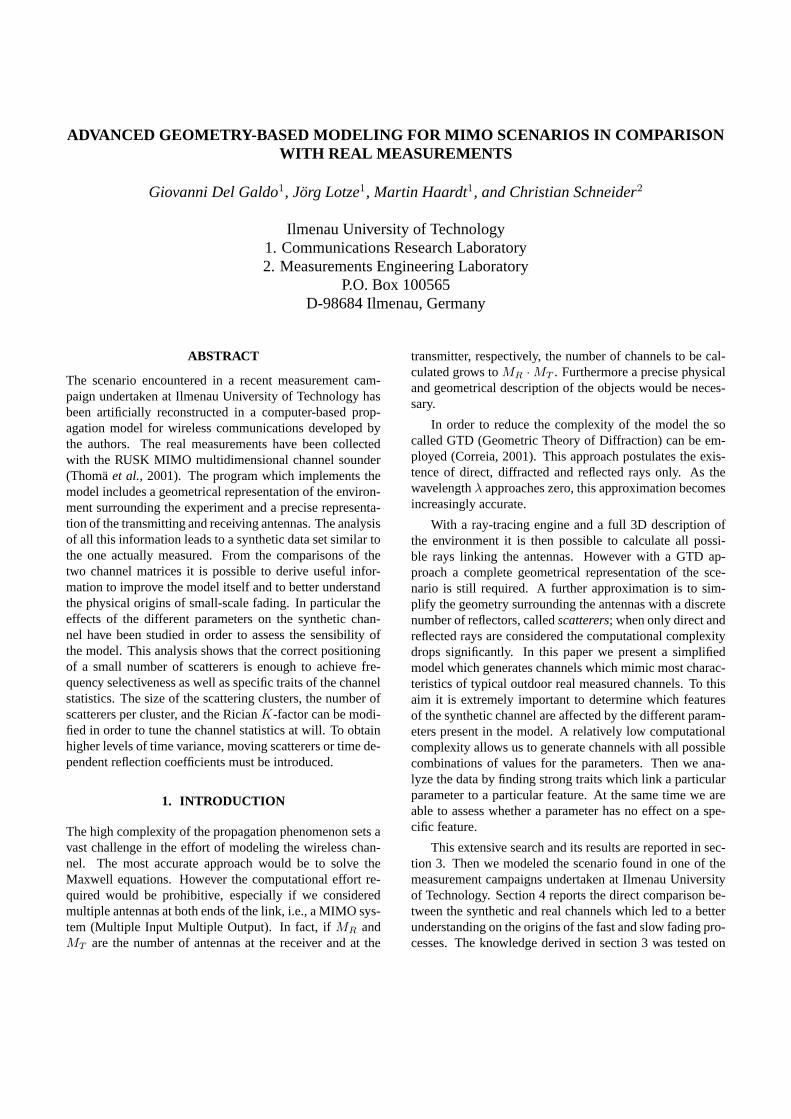
Fig. 10. The effective diversity order Ndiv plotted againstfrequency f for different cluster sizes (expressed in λ’s) forMβ .

in λ’s for the first model, Mα. Analyzing Ndiv along dif-ferent frequencies we can recognize a slow-moving trendcorrupted by faster variations. For instance, in the first plotof figure 10 (cluster size = 0.5 λ), we see a slow movingtrend which looks like a concave semicircle summed by azero mean noise-like process which introduces fast varia-tions. After many simulations we observed that the magni-tude of the fast moving Ndiv changed at every realizationwhile the variance of the slow moving Ndiv changed withthe cluster diameter with an undoubtedly direct proportion-ality. In other words, for bigger cluster sizes, Ndiv changesmore rapidly along frequency while this does not neces-sarily correspond to higher frequency selectiveness nor togreater time variance. The number of scatterers affects thechannel in a similar way but with a much weaker depen-dency.

4. A COMPARISON WITH REALMEASUREMENTS

In order to assess the results derived in section 3 with aneven more realistic scenario we modeled the surroundingsof a measurement campaign undertaken at TU Ilmenau. Ad-ditionally the simulation allowed us to investigate the im-portance of other critical parameters of the model: the posi-tions of the scatterers and the modeling of the reflection co-efficients. The first step was to determine whether a roughpositioning of the scatterers was enough to recreate the mainfeatures which characterize the measured channel. To thisend, we chose, among the many measurements gathered, achannel with a strong LOS and characterized by a simplegeometry so that the position of the scatterers could eas-

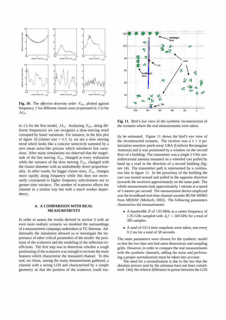
Fig. 11. Bird’s eye view of the synthetic reconstruction ofthe scenario where the real measurements were taken.

ily be estimated. Figure 11 shows the bird’s eye view ofthe reconstructed scenario. The receiver was a 4 × 8 po-larization sensitive patch-array URA (Uniform RectangularAntenna) and it was positioned by a window on the secondfloor of a building. The transmitter was a single 2 GHz om-nidirectional antenna mounted on a wheeled cart pulled byhand up a road in the direction of a second building (fig-ure 14). The transmitter path is represented by a continu-ous line in figure 11. In the proximity of the building thecart was turned around and pulled in the opposite direction(towards the receiver) approximately on the same path. Thewhole measurement took approximately 1 minute at a speedof 3 meters per second. The measurement device employedwas the broadband real-time channel sounder RUSK MIMOfrom MEDAV (Molisch, 2002). The following parameterscharacterize the measurements:

• A bandwidth B of 120 MHz at a center frequency of1.95 GHz sampled with ∆f = 300 kHz for a total of385 samples.

• A total of 6313 time snapshots were taken, one every9.2 ms for a total of 58 seconds.

The same parameters were chosen for the synthetic modelso that the two data sets had same dimensions and samplinggrids. However, in order to compare the real measurementswith the synthetic channels, adding the noise and perform-ing a proper normalization must be taken into account.

The need for a normalization is due to the fact that theabsolute powers sent by the antennas have not been consid-ered. Only the relative difference in power between the LOS

delay time [µs]

dela

y tim

e [s

]

0 0.5 1 1.5 2 2.5 3

0

10

20

30

40

50

−90

−80

−70

−60

−50

−40

−30

LOS

double−bounceecho

single−bounceecho

Fig. 12. Channel Impulse Responses from the real measure-ments in time t and delay time τ . The Line Of Sight LOSand echos are clearly visible. The grayscale represents am-plitudes in a dB scale

and the scattering components have been modeled throughthe Rician K -factor which can be set at will. This simpli-fied the modeling effort even though the results need post-processing in order to be finally compared with real mea-surements. The normalization is performed in such a waythat the total power received for the synthetic channel matchesthe one received in the measurements. Clearly both datasets must have the same number of samples, dimensions andmore in general, the same sampling grids. If HR denotesthe channel for the real measurements and HM the syn-thetic one then the whole channel matrix must be scaled sothat

∑

Θ

|HR|2 =∑

Θ

|HM |2 (12)

where Θ spans the complete domain of all dimensions. Inour simulations HM has been generated without noise. Thenormalization and the adding of the noise must then be doneconcurrently. First we have to estimate the power of thenoise from the measurements. We assume constant AWGN(Additive White Gaussian Noise) over all dimensions (de-lay time, time, antennas, etc.). An effective way to measurethe noise floor in the measurements is to observe the chan-nel matrix in the time and delay time domain. If the pathlengths are short enough, so that the last echoes extinguishbefore the maximum delay resolvable, we have a measure-ment of the noise without signal. If the number of samplesis sufficient we can use this data to estimate the power ofthe noise. The noisy synthetic channel will then be

HM ,noisy = HM ,noiseless + Hw, (13)

where Hw is a matrix whose elements are ZMCSCG (ZeroMean Circular Symmetric Complex Gaussians) random num-bers with variance σ2.

delay time [µs]

dela

y tim

e [s

]

0 0.5 1 1.5 2 2.5 3

0

10

20

30

40

50

−90

−80

−70

−60

−50

−40

−30

Fig. 13. The synthetically generated Channel Impulse Re-sponses in time t and delay time τ .

Equation (12) then becomes:∑

Θ

|HR|2 − γ · σ2 =∑

Θ

|HM |2, (14)

where γ is the total number of samples present in H , i.e.,γ = MR ×MT × T × F , where T and F are the numberof time snapshots and frequency bins respectively.

The geometry has been roughly reconstructed with thehelp of blueprints of the area and through visual inspection.Cars, buildings, light poles, and trash bins have been identi-fied as the probable sources of scattering. Figure 12 showsthe channel impulse responses in time t and delay time τ .The channel has been gathered originally in the {t, f} do-main; the CIRs in delay time have been computed via theFourier transform described in equation (1). The LOS isclearly visible and as expected its delay lag grows as thetransmitter moves farther away from the receiver. When thecart is turned around and pulled back towards the receiver,the arrival delay time decreases. Many echoes are visibleas well. Note that as the transmitter moves most echoes ar-rive earlier, meaning that their path length becomes smaller.When the curve corresponding to one echo changes in timewith the same slope characterizing the Line Of Sight, thenwe can deduce that the path length of the echo changes withthe same rate of the path length of the LOS. The strongecho labeled double-bounce echo has the same trend as theLOS just delayed by approximately 0.8 µs, which corre-sponds to 240 m, the distance between the top and bot-tom buildings doubled. For this reason it is very likelythat this arrival corresponds to the signal reflected by thebottom building first, and then by the top building, thus adoble-bounce echo. Figure 13 shows the channel generatedby our model. The trend of the LOS is extremely well re-produced. This was, however, expected since the LOS is

Fig. 14. The receiver (top circle) and the transmitting an-tenna (bottom circle) mounted on a cart.

the only component easily predictable once the position ofthe transmitter in known. Most of the scattering contribu-tions can be observed in the synthetic data set as well, withthe exception of the double-bounce paths which have beenomitted. Analyzing the two data sets in the {t, τ} domainsuggests improvements in the modeling approach: in thereal measurements we can observe that certain echo tracesare stronger than others. In the modeled channel this doesnot happen. This is a result of the modeling of the reflec-tion coefficients. In fact while their phase has been gener-ated uniformly distributed in the [0, 2π] range, the amplitudehas been taken equal for all. The comparison suggests thatthe reflection coefficients need a more sophisticated descrip-tion. Furthermore, a closer look on the real measurementsreveals that some echoes exist only in certain time periods.This suggests that the amplitude of the reflection coeffi-cients (perhaps their phases too) should be dependent on theDirection of Arrival and Direction of Departure (DoA andDoD). Figure 15 shows the fluctuations of the amplitudesof the channel for a specific frequency fo plotted againsttime for the first 25 seconds. Fast-fading characterizes bothsignals even though the real measurements appear some-how more variant. In order to assess this feature quanti-tatively we compute the multipath intensity profile ψDe(τ),the Doppler power spectrum ψDo(fD) and the autocorre-lation functions in frequency acf(∆f) and time acf(∆t)for both data sets. From their analysis we can obtain theRMS delay spread τRMS, the coherence bandwidth (∆f)c,the RMS Doppler spread fD,RMS and the coherence time(∆t)c (figures 16 and 17). The RMS delay spread showsthat the energy is similarly distributed in delay time τ . Inthe real measurements two more spikes can be observed.This is due to the fact that two specific echoes have a signif-icantly stronger magnitude compared to other echoes. TheRMS delay spread τRMS is anyhow very similar suggesting

0 5 10 15 20 25−50

−45

−40

−35

−30

−25

Am

plitu

de [d

B]

0 5 10 15 20 25−50

−45

−40

−35

−30

−25

Am

plitu

de [d

B]

time [s]

Fig. 15. Amplitudes of the CIRs for a specific frequency binplotted in dB against time for the real measurements (top)and the model (bottom).

that the two channels will have a similar frequency selec-tiveness. The RMS delay spread corresponds to the distancebetween the two vertical lines plotted in figures 16 and 17.From the autocorrelation function in the frequency domainacf(∆f) we can derive the coherence bandwidth (∆f)cwhich confirms that the two channels have approximatelythe same coherence bandwidth. In the {t, fD} pair the twochannels show more differences. While the Doppler powerspectrum ψDo(fD) has very similar trends, the autocorrela-tion function in the time domain shows that the measuredchannel is much more time variant than the synthetic one.Furthermore this analysis proves that equation (8) only rep-resents a good empirical law, valid in most but not all cases.In figure 15 we can in fact recognize that the real measure-ments have a faster moving small-fading effect, especiallyduring the first 10 seconds. We then investigated how wecould generate more time variance changing only positions,the size of the scattering clusters, and the number of scat-terers per cluster, and discovering that this was not possible.Our simulations showed that in order to achieve higher or-der of time variance it is absolutely necessary to model timevariant reflection coefficients or to introduce moving scat-terers along the time dimension.

5. CONCLUSIONS

Our simulations show that for certain modeling applicationsa simple GTD single-bounce model can mimic most chan-nel features with sufficient precision, among which the fre-quency selectiveness and the time variance are the mostcharacterizing. A rough positioning of the scattering clus-ters allows us to achieve a desired frequency selectivenessas well as other specific traits of the channel statistics by

0 1 2 3 4 5

x 10−7

0

1

2x 10

−10

delay time

ψ D

e(τ)

−40 −20 0 20 400

0.2

0.4

0.6

0.8

1x 10

−10

Doppler Frequency

ψ D

o(fD

)

−4 −2 0 2 4

x 106

0

0.2

0.4

0.6

0.8

1

frequency

acf(

∆f)

−0.1 −0.05 0 0.05 0.10

0.2

0.4

0.6

0.8

1

time

acf(

∆t)

Fig. 16. The multipath intensity profile ψDe(τ), Dopplerpower spectrum ψDo(fD) and the autocorrelation functionsin frequency acf(∆f) and time acf(∆t) for the real mea-surements

tuning three basic parameters, i.e, the size of the scatter-ing clusters, the number of scattering coefficients, and theRician K-factor. To obtain higher levels of time varianceand more realistic synthetic channels, moving scatterers andtime dependent reflection coefficients must be modeled aswell.

Acknowledgments

The authors gratefully acknowledge the support of MEDAV(www.channelsounder.de) in performing the channel mea-surements.

6. REFERENCES

A. Paulraj, R. Nabar and D. Gore (2003). Introduction tospace-time wireless communications. Cambridge Uni-versity Press. Cambridge.

Bello, P. (1963). Characterization of randomly time-variantlinear channels. IEEE Trans. Comm. Syst. 11, 360–393.

Correia, Luis M. (2001). Wireless Flexible PersonalisedCommunications. Wiley.

Molisch, A.F.; Steinbauer, M.; Toeltsch M.; Bonek E.;Thoma R.S. (2002). Capacity of MIMO systems basedon measured wireless channels. IEEE Journal on Se-lected Areas in Communications 20(3), 561–569.

Nabar, Rohit U. (2003). Performance Analysis and Transmit

0 1 2 3 4

x 10−7

0

0.5

1

1.5

x 10−10

delay time

ψ D

e(τ)

−40 −20 0 20 400

1

2x 10

−10

Doppler Frequency

ψ D

o(fD

)

−4 −2 0 2 4

x 106

0

0.2

0.4

0.6

0.8

1

frequency

acf(

∆f)

−0.2 −0.1 0 0.1 0.2 0.30

0.2

0.4

0.6

0.8

1

time

acf(

∆t)

Fig. 17. The multipath intensity profile ψDe(τ), Dopplerpower spectrum ψDo(fD) and the autocorrelation functionsin frequency acf(∆f) and time acf(∆t) for the model

Optimization for General MIMO Channels. DoctoralDissertation. Stanford.

Stuber, G. (1996). Principles of Mobile Communication.Kluwer. Norwell, MA.

Thoma, R.S., D. Hampicke, A. Richter, G. Sommerkorn andU. Trautwein (2001). MIMO vector channel soundermeasurement for smart antenna system evaluation. Eu-ropean Transaction on Telecommunications, Specialissue on smart antennas.