Snapshots from Transformation Geometry
99
Snapshots from Transformation Geometry Shailesh Shirali Community Mathematics Centre, Sahyadri School & Rishi Valley School (KFI) 29 November 2013, IMSc, Chennai SAS (CoMaC) Snapshots from Transformation Geometry Nov 2013 1 / 44
-
Upload
khangminh22 -
Category
Documents
-
view
0 -
download
0
Transcript of Snapshots from Transformation Geometry

Snapshots from Transformation Geometry
Shailesh Shirali
Community Mathematics Centre, Sahyadri School & Rishi Valley School (KFI)
29 November 2013, IMSc, Chennai
SAS (CoMaC) Snapshots from Transformation Geometry Nov 2013 1 / 44

What is geometry?
There are many different ways of defining ‘geometry’ but one of them is:
Geometry is the study of shapes, and how their properties are affected by
given groups of transformations: which properties are left unaltered, and
which ones undergo a change.
This view of geometry is due to the
mathematician Felix Klein (1849–1925).
SAS (CoMaC) Snapshots from Transformation Geometry Nov 2013 2 / 44

What is a ‘Geometric Transformation’?
A transformation of the plane is a function defined on the plane, moving
points around according to a definite law.
Matters of interest: Is the function ‘well behaved’? Is it smooth? Does it
preserve length? Angles? Orientation? Area?
In today’s talk we shall see how the use of transformations can give rise to
elegant proofs of some geometrical propositions.
SAS (CoMaC) Snapshots from Transformation Geometry Nov 2013 3 / 44

Affine maps
Let f be a bijection of the plane. We say that f is affine if it preserves the
property of collinearity. Let the images of points A, B, C , . . . under f be
A′, B′, C ′, . . .. Let the images of lines l , m under f be l ′, m′. Then:
SAS (CoMaC) Snapshots from Transformation Geometry Nov 2013 4 / 44

Affine maps
Let f be a bijection of the plane. We say that f is affine if it preserves the
property of collinearity. Let the images of points A, B, C , . . . under f be
A′, B′, C ′, . . .. Let the images of lines l , m under f be l ′, m′. Then:
• l ‖ m ⇐⇒ l ′ ‖ m′
• B is the midpoint of AC ⇐⇒ B′ is the midpoint of A′C ′
• A, B, C collinear =⇒ AB : BC = A′B′ : B′C ′
• Interior of △ABC is mapped to interior of △A′B′C ′
SAS (CoMaC) Snapshots from Transformation Geometry Nov 2013 4 / 44
Examples of affine maps
1 Isometries: mappings which preserve distance. Examples:
SAS (CoMaC) Snapshots from Transformation Geometry Nov 2013 5 / 44

Examples of affine maps
1 Isometries: mappings which preserve distance. Examples:
(a) Displacement (‘translation’) through a vector
SAS (CoMaC) Snapshots from Transformation Geometry Nov 2013 5 / 44

Examples of affine maps
1 Isometries: mappings which preserve distance. Examples:
(a) Displacement (‘translation’) through a vector
(b) Mirror reflection in a line
SAS (CoMaC) Snapshots from Transformation Geometry Nov 2013 5 / 44

Examples of affine maps
1 Isometries: mappings which preserve distance. Examples:
(a) Displacement (‘translation’) through a vector
(b) Mirror reflection in a line
(c) Rotation about a point, through some angle
SAS (CoMaC) Snapshots from Transformation Geometry Nov 2013 5 / 44

Examples of affine maps
1 Isometries: mappings which preserve distance. Examples:
(a) Displacement (‘translation’) through a vector
(b) Mirror reflection in a line
(c) Rotation about a point, through some angle
2 Enlargement about a point, by some scale factor (‘homothety’)
3 Shear
Note the progression: congruence geometry, similarity geometry, affine
geometry. This is in keeping with Klein’s vision.
SAS (CoMaC) Snapshots from Transformation Geometry Nov 2013 5 / 44

Notation
Symbol Meaning
TPQ
Translation (‘displacement’) through vector PQ
HP
Half-turn centred at point P
Mℓ Mirror reflection in line ℓ
RP,θ Rotation centred at P, through angle θ
EP,k
Enlargement centred at P, with scale factor k
Note: (i)(
TPQ
)−1= T
QP(ii) H
Pand M
ℓare self-inverse (iii) inverse of
RP,θ
is RP,−θ
(iv) inverse of EP,k
is EP,1/k
(v) EP,−1
is the same as HP
SAS (CoMaC) Snapshots from Transformation Geometry Nov 2013 6 / 44
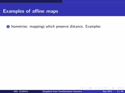
Composition of two reflections: parallel mirrors
If l ‖ m, then Ml followed by Mm is equivalent to a displacement.
l m
b b b
b b b
b bb
b b
A A′ A′′
B B′ B′′
C C′C′′
D D′ D′′
Segments AA′′, BB′′,
CC ′′, DD′′ have equal
length: each is twice the
distance between l & m.
SAS (CoMaC) Snapshots from Transformation Geometry Nov 2013 7 / 44

Composition of two reflections: non-parallel mirrors
If ¬(l ‖ m), then Ml followed by Mm is equivalent to a rotation.
b
b
b
b
Ol
m
A
A′
A′′
∠(l , O, m)
x
x
y
y
∠AOA′′ = 2 × ∠(l , O, m) = twice the directed angle from l to m
SAS (CoMaC) Snapshots from Transformation Geometry Nov 2013 8 / 44

Composition of two rotations
(With due apologies to Herr Klein)
b
b
A
B
I
II
III
RB,30◦
RA,60◦
Here we see a motif rotated
first about A by 60◦, then
about B by 30◦. From the
positions, it appears as though
a single rotation could have
taken the motif from I to III.
SAS (CoMaC) Snapshots from Transformation Geometry Nov 2013 9 / 44

Locating the centre of RB,β ◦ RA,α
A B
C
l
m
n
b b
b
12α
12β
12α + 1
2β
Draw line AB; draw lines m, n
through A, B such that
∠(m, l) = 12α, ∠(l , n) = 1
2β.
Keep directions in mind!
Let m, n meet at C . Then ∠(m, n) = 12α + 1
2β. So:
SAS (CoMaC) Snapshots from Transformation Geometry Nov 2013 10 / 44

Locating the centre of RB,β ◦ RA,α
A B
C
l
m
n
b b
b
12α
12β
12α + 1
2β
Draw line AB; draw lines m, n
through A, B such that
∠(m, l) = 12α, ∠(l , n) = 1
2β.
Keep directions in mind!
Let m, n meet at C . Then ∠(m, n) = 12α + 1
2β. So:
RA,α = Ml ◦ Mm, RB,β = Mn ◦ Ml ,

Locating the centre of RB,β ◦ RA,α
A B
C
l
m
n
b b
b
12α
12β
12α + 1
2β
Draw line AB; draw lines m, n
through A, B such that
∠(m, l) = 12α, ∠(l , n) = 1
2β.
Keep directions in mind!
Let m, n meet at C . Then ∠(m, n) = 12α + 1
2β. So:
RA,α = Ml ◦ Mm, RB,β = Mn ◦ Ml ,
∴ RB,β ◦ RA,α = (Mn ◦ Ml) ◦ (Ml ◦ Mm) .
SAS (CoMaC) Snapshots from Transformation Geometry Nov 2013 10 / 44
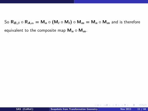
So RB,β ◦ RA,α = Mn ◦ (Ml ◦ Ml) ◦ Mm = Mn ◦ Mm and is therefore
equivalent to the composite map Mn ◦ Mm.
SAS (CoMaC) Snapshots from Transformation Geometry Nov 2013 11 / 44

So RB,β ◦ RA,α = Mn ◦ (Ml ◦ Ml) ◦ Mm = Mn ◦ Mm and is therefore
equivalent to the composite map Mn ◦ Mm.
But Mn ◦ Mm is equivalent to a rotation about the point where m and n
meet, through twice ∠(m, n).
SAS (CoMaC) Snapshots from Transformation Geometry Nov 2013 11 / 44

So RB,β ◦ RA,α = Mn ◦ (Ml ◦ Ml) ◦ Mm = Mn ◦ Mm and is therefore
equivalent to the composite map Mn ◦ Mm.
But Mn ◦ Mm is equivalent to a rotation about the point where m and n
meet, through twice ∠(m, n).
Therefore, RB,β ◦ RA,α is equivalent to the rotation RC ,α+β.
Could anything go wrong with this analysis? Yes: it could happen that
m ‖ n, in which case the lines m, n do not meet at all!
SAS (CoMaC) Snapshots from Transformation Geometry Nov 2013 11 / 44

This will happen if α + β is a multiple of 360◦.
However, the conclusion that RB,β ◦ RA,α = Mn ◦ Mm stays.
SAS (CoMaC) Snapshots from Transformation Geometry Nov 2013 12 / 44

This will happen if α + β is a multiple of 360◦.
However, the conclusion that RB,β ◦ RA,α = Mn ◦ Mm stays.
But since m ‖ n, the map Mn ◦ Mm is a displacement.
SAS (CoMaC) Snapshots from Transformation Geometry Nov 2013 12 / 44

This will happen if α + β is a multiple of 360◦.
However, the conclusion that RB,β ◦ RA,α = Mn ◦ Mm stays.
But since m ‖ n, the map Mn ◦ Mm is a displacement.
So if α + β is a multiple of 360◦, then RB,β ◦ RA,α is a displacement.
(Counterintuitive? Or daily life wisdom?)
SAS (CoMaC) Snapshots from Transformation Geometry Nov 2013 12 / 44

Part I
Problems and Theorems
We showcase some applications of the method of transformations.
SAS (CoMaC) Snapshots from Transformation Geometry Nov 2013 13 / 44

One of Euler’s (many) theorems
O: circumcentre, G: centroid, H: orthocentre;−→OH = 3
−→OG
bA
b
Bb
C
b
G
b
O
b
H
b
D
b EbF
→ △ABC , with circumcentre O,
centroid G , orthocentre H
→ D, E , F : midpoints of sides
→ Consider EG,−1/2:
SAS (CoMaC) Snapshots from Transformation Geometry Nov 2013 14 / 44

One of Euler’s (many) theorems
O: circumcentre, G: centroid, H: orthocentre;−→OH = 3
−→OG
bA
b
Bb
C
b
G
b
O
b
H
b
D
b EbF
→ △ABC , with circumcentre O,
centroid G , orthocentre H
→ D, E , F : midpoints of sides
→ Consider EG,−1/2: it maps
A, B, C to D, E , F .
SAS (CoMaC) Snapshots from Transformation Geometry Nov 2013 14 / 44

One of Euler’s (many) theorems
O: circumcentre, G: centroid, H: orthocentre;−→OH = 3
−→OG
bA
b
Bb
C
b
G
b
O
b
H
b
D
b EbF
→ △ABC , with circumcentre O,
centroid G , orthocentre H
→ D, E , F : midpoints of sides
→ Consider EG,−1/2: it maps
A, B, C to D, E , F . It maps
the perpr to BC through A to
the perpr to EF through D.
SAS (CoMaC) Snapshots from Transformation Geometry Nov 2013 14 / 44

One of Euler’s (many) theorems
O: circumcentre, G: centroid, H: orthocentre;−→OH = 3
−→OG
bA
b
Bb
C
b
G
b
O
b
H
b
D
b EbF
→ △ABC , with circumcentre O,
centroid G , orthocentre H
→ D, E , F : midpoints of sides
→ Consider EG,−1/2: it maps
A, B, C to D, E , F . It maps
the perpr to BC through A to
the perpr to EF through D. So
it maps H to O.
SAS (CoMaC) Snapshots from Transformation Geometry Nov 2013 14 / 44

One of Euler’s (many) theorems
O: circumcentre, G: centroid, H: orthocentre;−→OH = 3
−→OG
bA
b
Bb
C
b
G
b
O
b
H
b
D
b EbF
→ △ABC , with circumcentre O,
centroid G , orthocentre H
→ D, E , F : midpoints of sides
→ Consider EG,−1/2: it maps
A, B, C to D, E , F . It maps
the perpr to BC through A to
the perpr to EF through D. So
it maps H to O. It follows that−→OH = 3
−→OG.
SAS (CoMaC) Snapshots from Transformation Geometry Nov 2013 14 / 44

Two tangent circles
b
I
b
D
bA
b
O
b
E
b
Bb
C
→ Circles (I, A) and (O, A) touch
internally at A.
→ Chord BC of (O, A) is tangent
to (I, A) at D.
→ Point E lies on (O, A) such
that OE ⊥ BC .
→ Points A, D, E lie in a straight
line.
SAS (CoMaC) Snapshots from Transformation Geometry Nov 2013 15 / 44

Two more tangent circles
b
O
bK
b
I
bA b B
bC b D → Circles (I, K) and (O, K) touch
each other at K .
→ AB and CD are a pair of
parallel diameters of the two
circles (labeled suitably)
→ Points B, K, C lie in a straight
line, as do points A, K, D.
SAS (CoMaC) Snapshots from Transformation Geometry Nov 2013 16 / 44

An optimization problem
A nice use of transformations comes in solving the following problem first
studied by Fermat and Torricelli.
Problem
Given a triangle ABC , to find a point P in the plane of the triangle such
that PA + PB + PC has the least value possible.
We shall assume that no angle of the triangle exceeds 120◦.
SAS (CoMaC) Snapshots from Transformation Geometry Nov 2013 17 / 44

b
b
A
B C
D
P
Q
b
b b
b
→ P: candidate point.
→ Apply RC,60◦ : P 7→ Q, B 7→ D.
SAS (CoMaC) Snapshots from Transformation Geometry Nov 2013 18 / 44

b
b
A
B C
D
P
Q
b
b b
b
→ P: candidate point.
→ Apply RC,60◦ : P 7→ Q, B 7→ D.
→ △CPQ, △BDC : equilateral
SAS (CoMaC) Snapshots from Transformation Geometry Nov 2013 18 / 44

b
b
A
B C
D
P
Q
b
b b
b
→ P: candidate point.
→ Apply RC,60◦ : P 7→ Q, B 7→ D.
→ △CPQ, △BDC : equilateral
→ PC = PQ; PB = QD
SAS (CoMaC) Snapshots from Transformation Geometry Nov 2013 18 / 44

b
b
A
B C
D
P
Q
b
b b
b
→ P: candidate point.
→ Apply RC,60◦ : P 7→ Q, B 7→ D.
→ △CPQ, △BDC : equilateral
→ PC = PQ; PB = QD
→ PA + PB + PC = DQ + QP + PA
SAS (CoMaC) Snapshots from Transformation Geometry Nov 2013 18 / 44

b
b
A
B C
D
P
Q
b
b b
b
→ P: candidate point.
→ Apply RC,60◦ : P 7→ Q, B 7→ D.
→ △CPQ, △BDC : equilateral
→ PC = PQ; PB = QD
→ PA + PB + PC = DQ + QP + PA
→ PA + PB + PC ≥ DA
SAS (CoMaC) Snapshots from Transformation Geometry Nov 2013 18 / 44

b
b
A
B C
D
P
Q
b
b b
b
→ P: candidate point.
→ Apply RC,60◦ : P 7→ Q, B 7→ D.
→ △CPQ, △BDC : equilateral
→ PC = PQ; PB = QD
→ PA + PB + PC = DQ + QP + PA
→ PA + PB + PC ≥ DA
→ For equality: ∠APC , ∠BPC , ∠APB
all 120◦. These are the conditions for
P to be optimal.
SAS (CoMaC) Snapshots from Transformation Geometry Nov 2013 18 / 44

Fermat point of a triangle
b
A
B C
D
E
F
K
b
b b
b
b
b
→ △BDC , △CEA, △AFB:
equilateral
→ AD, BE , CF have equal length,
and they meet in the Fermat
point, K
→ AD, BE , CF make equal angles
with one another
SAS (CoMaC) Snapshots from Transformation Geometry Nov 2013 19 / 44
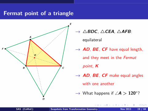
Fermat point of a triangle
b
A
B C
D
E
F
K
b
b b
b
b
b
→ △BDC , △CEA, △AFB:
equilateral
→ AD, BE , CF have equal length,
and they meet in the Fermat
point, K
→ AD, BE , CF make equal angles
with one another
→ What happens if ∠A > 120◦?
SAS (CoMaC) Snapshots from Transformation Geometry Nov 2013 19 / 44

What happens if ∠A > 120◦
A
B C
F
b Pb
Q
b
b b
b
→ P: candidate point
SAS (CoMaC) Snapshots from Transformation Geometry Nov 2013 20 / 44

What happens if ∠A > 120◦
A
B C
F
b Pb
Q
b
b b
b
→ P: candidate point
→ Apply RA,−60◦ . It maps P to Q &
B to F . Crucial: segment CF lies
‘outside’ the figure.
SAS (CoMaC) Snapshots from Transformation Geometry Nov 2013 20 / 44

What happens if ∠A > 120◦
A
B C
F
b Pb
Q
b
b b
b
→ P: candidate point
→ Apply RA,−60◦ . It maps P to Q &
B to F . Crucial: segment CF lies
‘outside’ the figure.
→ PA + PB + PC is equal to
CP + PQ + QF
SAS (CoMaC) Snapshots from Transformation Geometry Nov 2013 20 / 44

What happens if ∠A > 120◦
A
B C
F
b Pb
Q
b
b b
b
→ P: candidate point
→ Apply RA,−60◦ . It maps P to Q &
B to F . Crucial: segment CF lies
‘outside’ the figure.
→ PA + PB + PC is equal to
CP + PQ + QF
→ CP + PQ + QF ≥ CA + AF , so
d(P) ≥ d(A).
SAS (CoMaC) Snapshots from Transformation Geometry Nov 2013 20 / 44

What happens if ∠A > 120◦
A
B C
F
b Pb
Q
b
b b
b
→ P: candidate point
→ Apply RA,−60◦ . It maps P to Q &
B to F . Crucial: segment CF lies
‘outside’ the figure.
→ PA + PB + PC is equal to
CP + PQ + QF
→ CP + PQ + QF ≥ CA + AF , so
d(P) ≥ d(A). Hence A is the
optimizing point.
SAS (CoMaC) Snapshots from Transformation Geometry Nov 2013 20 / 44

Von Aubel’s quadrilateral theorem
bA
b
Bb
C
bD
bP
bQ
b R
b
S
b
b
b b
b
bb
b
→ Quadrilateral ABCD
→ Squares on its sides
→ Centres P, Q, R, S
SAS (CoMaC) Snapshots from Transformation Geometry Nov 2013 21 / 44

Von Aubel’s quadrilateral theorem
bA
b
Bb
C
bD
bP
bQ
b R
b
S
b
b
b b
b
bb
b
→ Quadrilateral ABCD
→ Squares on its sides
→ Centres P, Q, R, S
→ PR = QS, PR ⊥ QS
SAS (CoMaC) Snapshots from Transformation Geometry Nov 2013 21 / 44

bA
b
Bb
C
bD
bP
bQ
b R
b
S
b
M
→ Apply f = RP,90◦ , g = RQ,90◦ .
g ◦ f is a half-turn.
SAS (CoMaC) Snapshots from Transformation Geometry Nov 2013 22 / 44

bA
b
Bb
C
bD
bP
bQ
b R
b
S
b
M
→ Apply f = RP,90◦ , g = RQ,90◦ .
g ◦ f is a half-turn.
→ g ◦ f (B) = g(A) = D; so the
centre of g ◦ f is the midpoint
M of BD.
SAS (CoMaC) Snapshots from Transformation Geometry Nov 2013 22 / 44

bA
b
Bb
C
bD
bP
bQ
b R
b
S
b
M
→ Apply f = RP,90◦ , g = RQ,90◦ .
g ◦ f is a half-turn.
→ g ◦ f (B) = g(A) = D; so the
centre of g ◦ f is the midpoint
M of BD.
→ △PMQ is isosceles right-angled
at M. Same is true of △RMS.
SAS (CoMaC) Snapshots from Transformation Geometry Nov 2013 22 / 44

bA
b
Bb
C
bD
bP
bQ
b R
b
S
b
M
→ Apply f = RP,90◦ , g = RQ,90◦ .
g ◦ f is a half-turn.
→ g ◦ f (B) = g(A) = D; so the
centre of g ◦ f is the midpoint
M of BD.
→ △PMQ is isosceles right-angled
at M. Same is true of △RMS.
→ Now apply h = RM,90◦ . It maps
Q to P, S to R. Hence it maps
QS to PR. Hence etc.
SAS (CoMaC) Snapshots from Transformation Geometry Nov 2013 22 / 44

Napoleon’s theorem
b
b b
b
b
b
b
b
b
b
b
b
b
b
b
b
b b
b
b
b
A
B C
X
Y
Z
D
E
F
→ △ABC : arbitrary
→ △BXC , △CYA,
△AZB: equilateral
→ D, E , F : their centroids
(respectively); then:
→ △DEF is equilateral
SAS (CoMaC) Snapshots from Transformation Geometry Nov 2013 23 / 44

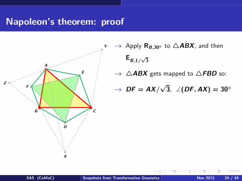
Napoleon’s theorem: proof
b
b b
b
b
b
b
b
b
b
b
b
b
b
b
b
b b
b
b
b
b
b
A
B C
X
Y
Z
D
E
F
→ Apply RB,30◦ to △ABX , and then
EB,1/
√3
SAS (CoMaC) Snapshots from Transformation Geometry Nov 2013 24 / 44

Napoleon’s theorem: proof
b
b b
b
b
b
b
b
b
b
b
b
b
b
b
b
b b
b
b
b
b
b
A
B C
X
Y
Z
D
E
F
→ Apply RB,30◦ to △ABX , and then
EB,1/
√3
→ △ABX gets mapped to △FBD so:
SAS (CoMaC) Snapshots from Transformation Geometry Nov 2013 24 / 44
Napoleon’s theorem: proof
b
b b
b
b
b
b
b
b
b
b
b
b
b
b
b
b b
b
b
b
b
b
A
B C
X
Y
Z
D
E
F
→ Apply RB,30◦ to △ABX , and then
EB,1/
√3
→ △ABX gets mapped to △FBD so:
→ DF = AX/√
3, ∠(DF , AX) = 30◦
SAS (CoMaC) Snapshots from Transformation Geometry Nov 2013 24 / 44

Napoleon’s theorem: proof
b
b b
b
b
b
b
b
b
b
b
b
b
b
b
b
b b
b
b
b
b
b
A
B C
X
Y
Z
D
E
F
→ Apply RB,30◦ to △ABX , and then
EB,1/
√3
→ △ABX gets mapped to △FBD so:
→ DF = AX/√
3, ∠(DF , AX) = 30◦
→ Apply RC,−30◦ to △ACX , then
EC,1/
√3.
SAS (CoMaC) Snapshots from Transformation Geometry Nov 2013 24 / 44

Napoleon’s theorem: proof
b
b b
b
b
b
b
b
b
b
b
b
b
b
b
b
b b
b
b
b
b
b
A
B C
X
Y
Z
D
E
F
→ Apply RB,30◦ to △ABX , and then
EB,1/
√3
→ △ABX gets mapped to △FBD so:
→ DF = AX/√
3, ∠(DF , AX) = 30◦
→ Apply RC,−30◦ to △ACX , then
EC,1/
√3. We get: DE = AX/
√3
and ∠(DE , AX) = −30◦. So:
SAS (CoMaC) Snapshots from Transformation Geometry Nov 2013 24 / 44
Napoleon’s theorem: proof
b
b b
b
b
b
b
b
b
b
b
b
b
b
b
b
b b
b
b
b
b
b
A
B C
X
Y
Z
D
E
F
→ Apply RB,30◦ to △ABX , and then
EB,1/
√3
→ △ABX gets mapped to △FBD so:
→ DF = AX/√
3, ∠(DF , AX) = 30◦
→ Apply RC,−30◦ to △ACX , then
EC,1/
√3. We get: DE = AX/
√3
and ∠(DE , AX) = −30◦. So:
→ DE = DF , ∠(DF , DE) = 60◦
SAS (CoMaC) Snapshots from Transformation Geometry Nov 2013 24 / 44

Napoleon’s theorem: proof
b
b b
b
b
b
b
b
b
b
b
b
b
b
b
b
b b
b
b
b
b
b
A
B C
X
Y
Z
D
E
F
→ Apply RB,30◦ to △ABX , and then
EB,1/
√3
→ △ABX gets mapped to △FBD so:
→ DF = AX/√
3, ∠(DF , AX) = 30◦
→ Apply RC,−30◦ to △ACX , then
EC,1/
√3. We get: DE = AX/
√3
and ∠(DE , AX) = −30◦. So:
→ DE = DF , ∠(DF , DE) = 60◦
→ Hence △DEF is equilateral
SAS (CoMaC) Snapshots from Transformation Geometry Nov 2013 24 / 44

Napoleon’s theorem: second proof
b
b b
b
b
b
b
b
b
b
b
b
b
b
b
b
b b
b
b
b
b
b
A
B C
X
Y
Z
D
E
F
→ ∠BFA = ∠AEC = ∠CDB = 120◦,
and 3 × 120◦ = 360◦
SAS (CoMaC) Snapshots from Transformation Geometry Nov 2013 25 / 44
Napoleon’s theorem: second proof
b
b b
b
b
b
b
b
b
b
b
b
b
b
b
b
b b
b
b
b
b
b
A
B C
X
Y
Z
D
E
F
→ ∠BFA = ∠AEC = ∠CDB = 120◦,
and 3 × 120◦ = 360◦
→ Let f = RD,120◦ ◦ RE,120◦ ◦ RF ,120◦ ;
f maps B to itself. Hence f = Id .
SAS (CoMaC) Snapshots from Transformation Geometry Nov 2013 25 / 44

Napoleon’s theorem: second proof
b
b b
b
b
b
b
b
b
b
b
b
b
b
b
b
b b
b
b
b
b
b
A
B C
X
Y
Z
D
E
F
→ ∠BFA = ∠AEC = ∠CDB = 120◦,
and 3 × 120◦ = 360◦
→ Let f = RD,120◦ ◦ RE,120◦ ◦ RF ,120◦ ;
f maps B to itself. Hence f = Id .
→ Hence RE,120◦ ◦ RF ,120◦ = RD,240◦
SAS (CoMaC) Snapshots from Transformation Geometry Nov 2013 25 / 44
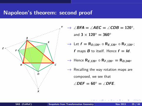
Napoleon’s theorem: second proof
b
b b
b
b
b
b
b
b
b
b
b
b
b
b
b
b b
b
b
b
b
b
A
B C
X
Y
Z
D
E
F
→ ∠BFA = ∠AEC = ∠CDB = 120◦,
and 3 × 120◦ = 360◦
→ Let f = RD,120◦ ◦ RE,120◦ ◦ RF ,120◦ ;
f maps B to itself. Hence f = Id .
→ Hence RE,120◦ ◦ RF ,120◦ = RD,240◦
→ Recalling the way rotation maps are
composed, we see that
∠DEF = 60◦ = ∠DFE .
→ Hence △DEF is equilateral
SAS (CoMaC) Snapshots from Transformation Geometry Nov 2013 25 / 44

Napoleon’s theorem: generalized version
b
b
b
b
b
b
b
b b
b
b
b
A
B C
D
E
F
→ △ABC : arbitrary
→ △BDC , △CEA, △AFB: all
isosceles, with apex angles α, β, γ
(resp), α + β + γ = 360◦; then:
SAS (CoMaC) Snapshots from Transformation Geometry Nov 2013 26 / 44

Napoleon’s theorem: generalized version
b
b
b
b
b
b
b
b b
b
b
b
A
B C
D
E
F
→ △ABC : arbitrary
→ △BDC , △CEA, △AFB: all
isosceles, with apex angles α, β, γ
(resp), α + β + γ = 360◦; then:
→ △DEF has angles α/2, β/2, γ/2
(resp)
SAS (CoMaC) Snapshots from Transformation Geometry Nov 2013 26 / 44

Napoleon’s theorem: generalized version
b
b
b
b
b
b
b
b b
b
b
b
A
B C
D
E
F
→ △ABC : arbitrary
→ △BDC , △CEA, △AFB: all
isosceles, with apex angles α, β, γ
(resp), α + β + γ = 360◦; then:
→ △DEF has angles α/2, β/2, γ/2
(resp)
→ Proof: Immediate . . .
SAS (CoMaC) Snapshots from Transformation Geometry Nov 2013 26 / 44
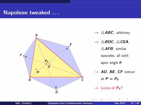
Napoleon tweaked . . .
A
B C
b
b b
b
D
θ
bE
θ
bFθ
bPθ
b
H
b
G
→ △ABC : arbitrary
→ △BDC , △CEA,
△AFB: similar
isosceles, all with
apex angle θ
→ AD, BE , CF concur
at P = Pθ
→ Locus of Pθ?
SAS (CoMaC) Snapshots from Transformation Geometry Nov 2013 27 / 44

Kiepert hyperbola
A
B C
b
b b
b
D
θ
bE
θ
bFθ
bPθ
b
H
b
G
b
The locus of Pθ is a
rectangular hyperbola
which passes through A,
B, C , H and G (here H
is the orthocentre and G
the centroid of △ABC)!
SAS (CoMaC) Snapshots from Transformation Geometry Nov 2013 28 / 44
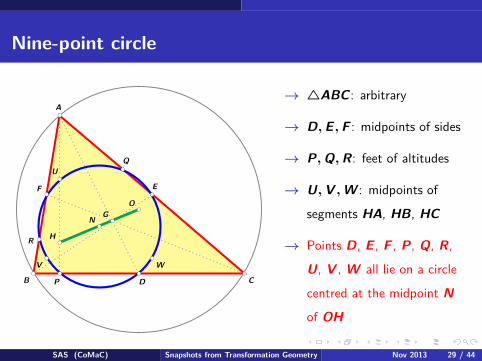
Nine-point circle
bcA
bcB
bcC
bc
D
bcE
bcF
bcH
bcG
bc
P
bcQ
bcR
bcO
bcU
bcV
bcW
bcN
→ △ABC : arbitrary
→ D, E , F : midpoints of sides
→ P, Q, R: feet of altitudes
→ U, V , W : midpoints of
segments HA, HB, HC
→ Points D, E , F , P, Q, R,
U, V , W all lie on a circle
centred at the midpoint N
of OH
SAS (CoMaC) Snapshots from Transformation Geometry Nov 2013 29 / 44

Basic idea for the proof
bcA bc Bbc
K
C1
C2
Given two circles C1, C2 of equal size,
sharing a chord AB, there are at least
two distinct isometric maps which map
one circle to the other:
→ Reflection in line AB
→ Half-turn about the midpoint K of
AB.
Notation: ω(ABC) denotes the circumcircle of △ABC , etc
SAS (CoMaC) Snapshots from Transformation Geometry Nov 2013 30 / 44

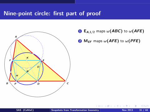
Nine-point circle: first part of proof
bcA
bcB
bcC
bc
D
bc EbcF
bc
H
bc
P
bc
bc
bc
Obc
N
bcK
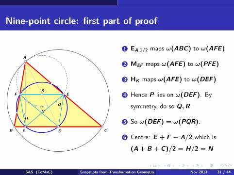
1 EA,1/2 maps ω(ABC) to ω(AFE)
SAS (CoMaC) Snapshots from Transformation Geometry Nov 2013 31 / 44
Nine-point circle: first part of proof
bcA
bcB
bcC
bc
D
bc EbcF
bc
H
bc
P
bc
bc
bc
Obc
N
bcK
1 EA,1/2 maps ω(ABC) to ω(AFE)
2 MEF maps ω(AFE) to ω(PFE)
SAS (CoMaC) Snapshots from Transformation Geometry Nov 2013 31 / 44

Nine-point circle: first part of proof
bcA
bcB
bcC
bc
D
bc EbcF
bc
H
bc
P
bc
bc
bc
Obc
N
bcK
1 EA,1/2 maps ω(ABC) to ω(AFE)
2 MEF maps ω(AFE) to ω(PFE)
3 HK maps ω(AFE) to ω(DEF)
SAS (CoMaC) Snapshots from Transformation Geometry Nov 2013 31 / 44

Nine-point circle: first part of proof
bcA
bcB
bcC
bc
D
bc EbcF
bc
H
bc
P
bc
bc
bc
Obc
N
bcK
1 EA,1/2 maps ω(ABC) to ω(AFE)
2 MEF maps ω(AFE) to ω(PFE)
3 HK maps ω(AFE) to ω(DEF)
4 Hence P lies on ω(DEF). By
symmetry, do so Q, R.
SAS (CoMaC) Snapshots from Transformation Geometry Nov 2013 31 / 44

Nine-point circle: first part of proof
bcA
bcB
bcC
bc
D
bc EbcF
bc
H
bc
P
bc
bc
bc
Obc
N
bcK
1 EA,1/2 maps ω(ABC) to ω(AFE)
2 MEF maps ω(AFE) to ω(PFE)
3 HK maps ω(AFE) to ω(DEF)
4 Hence P lies on ω(DEF). By
symmetry, do so Q, R.
5 So ω(DEF) = ω(PQR).
SAS (CoMaC) Snapshots from Transformation Geometry Nov 2013 31 / 44
Nine-point circle: first part of proof
bcA
bcB
bcC
bc
D
bc EbcF
bc
H
bc
P
bc
bc
bc
Obc
N
bcK
1 EA,1/2 maps ω(ABC) to ω(AFE)
2 MEF maps ω(AFE) to ω(PFE)
3 HK maps ω(AFE) to ω(DEF)
4 Hence P lies on ω(DEF). By
symmetry, do so Q, R.
5 So ω(DEF) = ω(PQR).
6 Centre: E + F − A/2 which is
(A + B + C)/2 = H/2 = N
SAS (CoMaC) Snapshots from Transformation Geometry Nov 2013 31 / 44

Nine-point circle: second part of proof
bcA
bcB
bcC
bc
D
bc EbcF
bc
H
bc
P
bcQ
bcR
bc
O
bcU
bcV
bcW
bc
N
bcK
1 EH,1/2 maps ω(ABC) to
ω(UVW )
SAS (CoMaC) Snapshots from Transformation Geometry Nov 2013 32 / 44

Nine-point circle: second part of proof
bcA
bcB
bcC
bc
D
bc EbcF
bc
H
bc
P
bcQ
bcR
bc
O
bcU
bcV
bcW
bc
N
bcK
1 EH,1/2 maps ω(ABC) to
ω(UVW )
2 Hence the centre of ω(UVW ) is
H/2 = N, and its radius is half
the radius of ω(ABC)
SAS (CoMaC) Snapshots from Transformation Geometry Nov 2013 32 / 44

Nine-point circle: second part of proof
bcA
bcB
bcC
bc
D
bc EbcF
bc
H
bc
P
bcQ
bcR
bc
O
bcU
bcV
bcW
bc
N
bcK
1 EH,1/2 maps ω(ABC) to
ω(UVW )
2 Hence the centre of ω(UVW ) is
H/2 = N, and its radius is half
the radius of ω(ABC)
3 Hence ω(UVW ) coincides with
ω(DEF) and ω(PQR).
SAS (CoMaC) Snapshots from Transformation Geometry Nov 2013 32 / 44
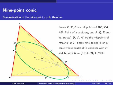
Nine-point conic
Generalization of the nine-point circle theorem
bcA
bcB
bcC
bc
D
bc EbcF
bcG
bcH
bc
P
bcQ
bcRbc
U
bcV
bc W
bcN
Points D, E , F are midpoints of BC , CA,
AB. Point H is arbitrary, and P, Q, R are
its ‘traces’. U, V , W are the midpoints of
HA, HB, HC . These nine points lie on a
conic whose centre N is collinear with H
and G, with N = (3G + H)/4. Well!
SAS (CoMaC) Snapshots from Transformation Geometry Nov 2013 33 / 44

Part II
Frieze Patterns
SAS (CoMaC) Snapshots from Transformation Geometry Nov 2013 34 / 44
Mosaic
Human beings have used mosaic as an art form for centuries. The Islamic
cultures in particular have developed this art form to a very high level.
SAS (CoMaC) Snapshots from Transformation Geometry Nov 2013 35 / 44

Mosaic
Human beings have used mosaic as an art form for centuries. The Islamic
cultures in particular have developed this art form to a very high level.
Mosaic can be one dimensional, as in a frieze pattern, or two dimensional,
as in wallpaper or floor tilings.
The most stunning exhibitions of tiling patterns are seen in the Alhambra
Palace in Granada, Spain.
SAS (CoMaC) Snapshots from Transformation Geometry Nov 2013 35 / 44
The seven frieze patterns
Frieze patterns are all around us (look around you and check this out).
It can be shown that the underlying symmetry group of a frieze pattern is
one of just seven possibilities.
This may come as a surprise, but it can be proved. The individual details
of the motifs used in the pattern may differ, but the symmetry groups are
just seven in number.
We take a quick look at these seven possibilities.
SAS (CoMaC) Snapshots from Transformation Geometry Nov 2013 36 / 44

Translations only
Frieze pattern type T : . . . F F F F F F F . . .
SAS (CoMaC) Snapshots from Transformation Geometry Nov 2013 37 / 44

Translations and horizontal axis reflection
Frieze pattern type TX : . . . B B B B B B B . . .
SAS (CoMaC) Snapshots from Transformation Geometry Nov 2013 38 / 44

Translations and vertical axis reflection
Frieze pattern type TY : . . . A A A A A A A . . .
SAS (CoMaC) Snapshots from Transformation Geometry Nov 2013 39 / 44
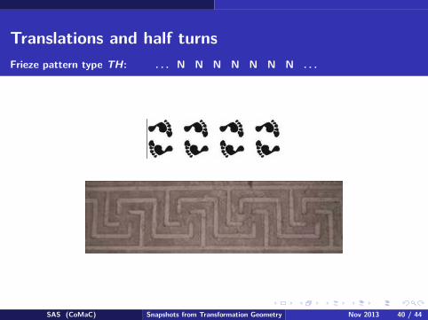
Translations and half turns
Frieze pattern type TH: . . . N N N N N N N . . .
SAS (CoMaC) Snapshots from Transformation Geometry Nov 2013 40 / 44

Translations and horizontal and vertical reflections
Frieze pattern type THXY : . . . X X X X X X X . . .
SAS (CoMaC) Snapshots from Transformation Geometry Nov 2013 41 / 44

Translations and glide reflections
Frieze pattern type TG: . . . b p b p b p b p . . .
SAS (CoMaC) Snapshots from Transformation Geometry Nov 2013 42 / 44

Translations and vertical reflections + glides
Frieze pattern type TGY : . . . p q b d p q b d p q b d p q . . .
SAS (CoMaC) Snapshots from Transformation Geometry Nov 2013 43 / 44
Max Jeger, Transformation Geometry (1966)
E A Maxwell, Geometry By Transformations (Cambridge Univ Press,
SMP)
I M Yaglom, Geometric Transformations I and Geometric
Transformations II (MAA)
SAS (CoMaC) Snapshots from Transformation Geometry Nov 2013 44 / 44