Adaptive spatial combining for passive time-reversed communications

Adaptive spatial combining for passive time-reversedcommunicationsa)

João Gomesb�

Institute for Systems and Robotics, Instituto Superior Técnico, 1049-001 Lisboa, Portugal

António Silvac� and Sérgio Jesusd�

Institute for Systems and Robotics, Universidade do Algarve, Campus de Gambelas,8005-139 Faro, Portugal

�Received 5 April 2007; revised 27 May 2008; accepted 28 May 2008�

Passive time reversal has aroused considerable interest in underwater communications as acomputationally inexpensive means of mitigating the intersymbol interference introduced by thechannel using a receiver array. In this paper the basic technique is extended by adaptively weightingsensor contributions to partially compensate for degraded focusing due to mismatch between theassumed and actual medium impulse responses. Two algorithms are proposed, one of which restoresconstructive interference between sensors, and the other one minimizes the output residual as inwidely used equalization schemes. These are compared with plain time reversal and variants thatemploy postequalization and channel tracking. They are shown to improve the residual error andtemporal stability of basic time reversal with very little added complexity. Results are presented fordata collected in a passive time-reversal experiment that was conducted during the MREA’04 seatrial. In that experiment a single acoustic projector generated a 2 /4-PSK �phase-shift keyed� streamat 200 /400 baud, modulated at 3.6 kHz, and received at a range of about 2 km on a sparse verticalarray with eight hydrophones. The data were found to exhibit significant Doppler scaling, and aresampling-based preprocessing method is also proposed here to compensate for that scaling.© 2008 Acoustical Society of America. �DOI: 10.1121/1.2946711�

PACS number�s�: 43.60.Dh, 43.60.Tj, 43.60.Gk, 43.60.Fg �DRD� Pages: 1038–1053

I. INTRODUCTION

Time reversal is a wave backpropagation technique thatcleverly exploits the reciprocity of linear wave propagationto concentrate signals at desired points in a waveguide withlittle knowledge about the medium.1 The potential of timereversal for underwater communications was recognized andattracted much attention after the practical feasibility of thistechnique was demonstrated in the ocean.2

Active time-reversed �TR� focusing is achieved by trans-mitting a channel probe from the intended focal spot to anarray of transducers that sample the incoming pressure field.These signals are then reversed in time and retransmitted,creating a replica field that converges on the original sourcelocation and approximately regenerates the initial waveform, undoing much of the delay dispersion caused by mul-tipath. Due to its peculiar mode of operation, this type ofsource/receiver array is often referred to as a time-reversalmirror �TRM�. When the principle of time reversal is appliedto digital communications, the measured probe source ping ismodulated with an information-bearing wave form, whichcan then be demodulated at the focus with relatively lowalgorithmic complexity. Passive time reversal, or passivephase conjugation3 �PPC�, is conceptually similar to the

a�Portions of this work were presented at the MTS/IEEE Oceans’06 Confer-ence, Boston, MA, September 2006.

b�Electronic mail: [email protected]�Electronic mail: [email protected]�
Electronic mail: [email protected]
1038 J. Acoust. Soc. Am. 124 �2�, August 2008 0001-4966/2008/12

above technique, yet both the probe and message are sequen-tially sent from the source, so the array only operates inreceive mode. Focusing is performed synthetically at the ar-ray by convolving the time-reversed distorted probes withreceived data packets.3 This is, in fact, a multichannel com-bining �MC� strategy4 whose parameters are directly mea-sured from the data, not derived by optimizing a cost func-tion.

Time reversal finds applications in diverse areas such asoptics, materials testing, imaging, and medicine.5 In under-water acoustics, digital communications have provided thebackdrop for many published applications of this technique.In fact, the wave form regeneration property of TRM ishighly relevant in underwater acoustic communications,where intersymbol interference �ISI� caused by multipath isusually the single most important distortion to becompensated.4 Stojanovic6 provides an overview of much ofthe research work in this area.

Both active7,8 and passive9–11 TR communications havebeen demonstrated in the ocean, the latter being more popu-lar due to a simpler hardware setup. These experimental re-sults, and other theoretical analyses,6,12,13 suggest that timereversal by itself will not ensure reliable detection of thetransmitted symbols, and should be complemented by adap-tive equalization at the receiver to remove the residual ISIand compensate for channel variations. Arguably, the overall
reduction in computational complexity at the receiver af-
© 2008 Acoustical Society of America4�2�/1038/16/$23.00

forded by the integration of time reversal into an acousticlink more than makes up for the moderate degradation inperformance.

Most of the experiments reported to date employ single-carrier coherent signaling, although time reversal can easilybe adapted to other modulations as well.14 In fact, in linewith a popular trend in underwater communications, severaltechniques first developed in wireless terrestrial communica-tions have been investigated and proposed for acoustic linksbased on time reversal. This trend continues with multiple-input/multiple-output communications, which have providedlarge performance improvements in wireless radio and showgreat promise in underwater communications.15

In the methods that have been proposed so far for simul-taneous equalization and time reversal the two systems areoperated in tandem, i.e., a TRM creates a single-channel sig-nal which is then independently processed by anequalizer.6,12,16 In PPC, however, the signals received at anarray of hydrophones are synthetically combined after con-volving them with estimates of the �reversed� channel im-pulse responses. This provides increased flexibility relativeto active TR, as these signals may be individually postpro-cessed prior to generating a single-channel wave form.

This paper examines low-complexity PPC approacheswhere a single combining coefficient is used per array sensorto improve upon the performance of basic PPC under chan-nel variations. These coefficients are adjusted at each symbolinterval by either iteratively minimizing the output mean-square error �MSE� or maximizing the output magnitude.This approach is motivated by the observation that poorsignal-to-interference �ISI+noise� ratio that occurs due to en-vironment mismatch between the probe and packet transmis-sions can often be attributed to partially destructive interfer-ence between contributions from different hydrophonesignals, in spite of appropriate temporal alignment. Note thatthe proposed structures are actually very short multichannelequalizers, and one could envisage using more elaborate fil-ters as in conventional equalizers.

Environment mismatch is also addressed in decision-directed PPC17 �DDPPC� by tracking the channel impulseresponse continuously throughout a data packet to virtuallyeliminate the delay between probe capture and filtering. Itshould be emphasized that the MC methods proposed hereare simpler, as the probe is only captured during the packetpreamble, and subsequently only one coefficient per sensor istracked. By contrast, DDPPC must propagate a fully adap-tive model of the channel response measured in each sensor�or at least the portion of it with higher energy and greatertemporal stability�, which is not necessarily less computa-tionally demanding than conventional equalization schemes.

Results from a passive time-reversal experiment con-ducted off the west coast of Portugal during the MREA’04sea trial are presented. A single acoustic projector generateda 2 /4-PSK stream at 200 and 400 baud around a carrierfrequency of 3.6 kHz, and the signals were received at arange of about 2 km on a vertical array with eight unevenlyspaced hydrophones. The channel end points were in motionduring this experiment, inducing significant Doppler scaling
in the observed wave forms that could degrade the perfor-
J. Acoust. Soc. Am., Vol. 124, No. 2, August 2008 Gomes

mance of TR focusing if left uncompensated.11 A broadbandDoppler compensation method is proposed here, theoreti-cally analyzed, and shown to perform very effectively inpractice. The method itself is simple and similar ideas havebeen proposed in the past, but to the best of our knowledgeno prior analysis of Doppler compensation on TRM perfor-mance has been published. In addition to documenting theperformance of proposed MC algorithms, this work alsoaims to provide experimental results on various aspects ofchannel characterization, conventional equalization, andplain time reversal.

The paper is organized as follows. Section II introducesthe signal model used for time reversal and describes theDoppler compensation method. Section III presents the mul-tichannel combining algorithms, illustrates their performancein a simulated scenario, and discusses the synchronizationand normalization postprocessing steps that are required toestimate data symbols from the TRM output. Section IV de-scribes the MREA’04 sea trial and presents experimental re-sults. The proposed MC algorithms are characterized andcompared with plain multichannel equalization, plain TRM,simultaneous TRM and single-channel equalization, andDDPPC. Channel/probe estimation issues are also consid-ered. Finally, Sec. V summarizes the main results, drawssome conclusions, and suggests future research.

II. MODELING OF TIME REVERSAL

This section presents the notation used in the sequel forcoherent communication using time reversal. The reader isreferred to Refs. 1 and 2 for an overview of �narrowband� TRtheory, and to several references on �broadband� TRcommunications8,9,11 for lengthier discussions on specific as-pects of data transmission. Throughout the paper convolutionis denoted by the binary operator � and complex conjugationby the superscript �·�*.

As is usually done in the context of bandwidth-efficientcoherent communications, a complex representation in termsof baseband equivalent signals �i.e., complex envelopes� willhenceforth be adopted for the real passband wave forms thatare actually transmitted and received.18 Time reversal ofbandpass signals must then be replaced by time reversal andconjugation of complex envelopes, but other than that allequations describing the self-focusing property remain un-changed.

Let p�t� represent the ideal basic pulse shape of themodulated wave forms that are exchanged between thesource and the TRM, which can also act as a convenientchannel probe. Other wave forms used for channel identifi-cation, such as linear frequency modulated pulses, are alsoappropriate. Denoting by gm�t� the impulse response betweenthe focal point and the mth sensor of an M-element array, thedistorted received probe is hm�t�= p�t��gm�t�. In active timereversal the TRM then transmits an arbitrary data packetwith pulse shape h*�−t� which, by virtue of TR focusing, willbe approximately regenerated at the focal spot with the origi-nal pulse shape p*�−t�. In passive phase conjugation theprobe is followed by a data packet transmitted by the same
source after a guard interval. Coherent single-carrier modu-
et al.: Adaptive combining for time-reversed communications 1039

lation is assumed throughout this work, such that the re-ceived signal component at the mth sensor is given by

ym�t� = �k

a�k�hm�t − kTb� . �1�

In the complex baseband representation underlying Eq. �1�the information symbols �a�k��, transmitted with interval Tb,belong to a discrete signal constellation.18 This is defined asa finite set of points in the complex plane that representgroups of bits from a digital message. Physically, the real andimaginary components of a�k� are used for amplitude modu-lation of the in-phase and quadrature carriers when generat-ing real bandpass wave forms. The symbols �a�k�� are as-sumed to be uncorrelated random variables with zero meanand unit variance. The noise component will be ignored inthe characterization of time reversal given below.

A plain passive mirror emulates active time reversal syn-thetically in a receive-only array. Its output, z�t�, is obtainedby convolving the received packet �1� with the TR probereplica to generate a match-filtered signal in each sensor,zm�t�, and then adding all contributions

zm�t� = hm*�− t� � ym�t� , �2�

z�t� = �m=1

M

zm�t� = �k

a�k�q�t − kTb� . �3�

In Eq. �3� q�t� denotes the sum of temporal autocorrelationsof received pulse shapes, sometimes referred to as theq-function19 �QF�. In a static ocean environment it is relatedto the medium impulse responses as

q�t� = �m=1

M

hm*�− t� � hm�t� = r�t� � ��t� , �4�

where

r�t� = p*�− t� � p�t�, ��t� = �m=1

M

gm*�− t� � gm�t� . �5�

The multipath self-compensation property of time reversalimplies that the spectrum of ��t� should be approximatelyconstant across the bandwidth of p�t� �and r�t��, so thatq�t��r�t� and an undistorted modulated wave form is regen-erated. In practice a delay is introduced to ensure causality ofthe time-reversed probe in Eq. �2�, and all operations areperformed in L-oversampled discrete-time signals ym�n��ym�nTb /L� and hm�n�.

Decoding is particularly simple when p�t� has a rootraised-cosine shape because then r�t� in Eqs. �3� and �4� is aNyquist pulse.18 Out-of-band noise removal can be accom-plished by actually transmitting fourth-root raised-cosine sig-naling pulses10 s�t� such that p�t�=s*�−t��s�t�, and then pre-filtering all received wave forms �probes and packets� bys*�−t� to reject noise and attain the desired equivalent pulseshape p�t�. To avoid unnecessarily complicating our notationwe assume that hm and ym in Eqs. �1�, �2�, and �4� havealready undergone filtering by s*�−t�. The spectra of p�t�,
r�t�, and s�t� are then related by
1040 J. Acoust. Soc. Am., Vol. 124, No. 2, August 2008

P�� = R1/2��, S�� = R1/4��, R�� 0. �6�

Coherence issues. When channel variations occur be-tween the probe and packet transmissions, autocorrelationsin Eq. �4� are replaced by crosscorrelations between receivedpulses at different instants. This decreases the TRM’s focus-ing power by degrading the impulselike behavior of q�t�.

To reduce the latency and mismatch between probe mea-suring and focusing, it is possible to discard the actual probetransmission and estimate it directly from a known preamblein the data packet.16 This has the added benefit of reducingthe additive noise component in the probe estimate hm�t�,which generates undesirable convolutional noise during fo-cusing. In a nonstatic environment it may also filter out thecontributions from paths with poor temporal coherence, thusreducing the jitter in match-filtered outputs. This idea istaken further in DDPPC,17 where the channel is trackedthroughout data packets. A sharp QF is thus preserved evenwith very long packets because a low-latency channel esti-mate is always available.

The total number of parameters to be estimated byDDPPC in typical �multiple-hydrophone� discrete tap-delay-line models of underwater channels may be quite large andimpose a significant computational burden. Alternative strat-egies that perform simpler adaptation and require fewer pa-rameters, such as the ones addressed in this paper, may there-fore be of interest. While Flynn et al.17 argue in favor ofiterative block least-squares estimation, in this work weadopt the exponentially windowed recursive least-squares�RLS� algorithm for channel estimation and tracking, whichhas been extensively used in underwater channel equaliza-tion and identification.

A. Doppler distortion and compensation

By decomposing a source with arbitrary space-time de-pendence as a superposition of monochromatic pointsources, TR focusing may be shown to hold even for movingsources.1 This work addresses a restricted case where thesource is assumed to be moving slowly enough over a suffi-ciently short period so that the medium impulse responseslinking it to the array transducers remain approximately con-stant. TR experiments suggest that this hypothesis is moreplausible for predominantly horizontal motion, as the size ofthe focal spot in the horizontal plane is larger than along thedepth axis.

Given a nominal transmitted passband wave form withcarrier frequency �c, x�t�=Re�x�t�ej�ct�, the equivalentDoppler-distorted transmission over a single path is

x��1 + ��t� = Re�x��1 + ��t�ej�c�tej�ct� , �7�

where � is the time compression/dilation factor. For a mov-ing transmitter with velocity v heading toward a static re-ceiver in a medium with sound speed c�v, � is given by20

� =1

1 − v/c− 1 �

vc

. �8�

In terms of baseband signals, Eq. �7� amounts to time scalingof the original x�t� and multiplication by a complex exponen-
tial with angular frequency �c�. In a multipath environment
Gomes et al.: Adaptive combining for time-reversed communications

several delayed contributions of the above type are observedat the receiver, but if the propagation geometry and motionare predominantly horizontal, all scaling factors will be simi-lar and compensating for the average Doppler usually suf-fices. Scattering by suspended particles may complicate theobserved Doppler and multipath profiles, and is beyond thescope of this work.

Given an estimate of � the Doppler-compensated re-ceived signal is obtained from ym�t� as

ym� �t� = ym t

1 + �e−j�c��t/�1+��, �9�

and used in all subsequent TR processing. The correctness ofEq. �9� can be asserted for the Doppler-distorted complexenvelope of Eq. �7�, ym�t�=x��1+��t�ej�c�t, in which caseym� �t�=x�t� as intended. The same Doppler correction is ap-plied to received channel probes whenever they are avail-able. This operation, which is shown to preserve the sharp-ness of the QF in Sec. A 1, leads to equivalent pulse shapesand impulse responses that are much more convenient toprocess and visualize due to their comparatively low rate ofvariation in time. A similar resampling approach has beenproposed by Song et al.,11 but justified only heuristically.Alternative Doppler compensation methods are needed when� cannot be assumed constant over a packet duration, butthis hypothesis proved to be fully satisfactory for MREA’04data.

The type of Doppler processing proposed here bearssome resemblance to methods that have been proposed forvarying the focal range of an active TRM through frequencyshifting of a single captured probe.21,22 The approach relieson the fact that, for a given environment, nominal frequency� and range r, the ratio between �small� relative changes�� /� and �r /r is a constant known as the waveguide in-variant. In a broadband communications context this prop-erty implies that the channel impulse response between astatic source and a receiver at range �r+r approximatelyequals a time-scaled version of the nominal one.23 The Dop-pler processing method described above can then be inter-preted as follows: The packet transmission originating atrange r is time scaled at the TRM to compensate for Dopplercompression due to source motion, but this also rescales theunderlying impulse response and makes it appear as thoughthe source is positioned at a different range. Direct matchedfiltering using measured probes would then result in loss ofsharpness of the QF due to range mismatch. Time scaling ofchannel probes prior to filtering counters this effect by rep-licating exactly the same impulse response distortion intro-duced in data packets, so that the range mismatch vanishesand a sharply focused signal is again obtained.

III. MULTICHANNEL COMBINING

A sum of matched filters such as the one used in PPC isa known generic front end for optimal multichannel datareceivers under several criteria, including minimum MSE�Ref. 24� and minimum probability of sequence error underadditive white Gaussian noise.25 It should ideally be fol-
lowed by a single-channel receiver to deal with residual ISI.

Alternative strategies for multichannel equalization havebeen proposed for reducing the overall computational com-plexity or providing more flexibility when the channel re-sponses are imperfectly known at the receiver.1

Formal justification for the multipath compensationproperty can be found elsewhere,1,2,26 but intuitively it maybe understood as follows. Each term h

m*�−t��hm�t� in Eq. �3�

has a main lobe at time t=0 and �conjugate symmetrical�secondary lobes at other delays due to multipath. Main lobecontributions are all real, positive, and hence add up inphase. Secondary lobes, however, are not aligned in delayand phase for different sensors, and are not expected to re-inforce each other the way that the main lobes do. As aresult, an impulselike QF with dominating main lobeemerges as more and more terms are added. Perfect ISI re-moval through time reversal is only theoretically attained inthe limit as the number of individual multipaths and/or un-correlated receive elements gets very large.

The proposed multichannel combining algorithms arebased on the assumption that, for moderate mismatch, theconstructive interference of pulse contributions in q�0� ispartially lost even though the shapes of individual terms inthe summation are not severely affected with respect to thestatic case. It should then be possible to mitigate this effectby multiplying each term by a single complex coefficient wm

to restore the phase alignment at t=0. Denoting by hm� �t� theactual pulse shape during focusing that differs from the chan-nel probe hm�t�, the modified TRM output in the presence ofmismatch is given by

z�t� = �m=1

M

wmzm�t� = �k

a�k�q�t − kTb� , �10�

q�t� = �m=1

M

wmqm�t�, qm�t� = hm*�− t� � hm� �t� . �11�

In terms of symbol-rate-sampled variables in Eqs. �10� and�11�, z�n��z�nTb�, zm�n�, q�n�, qm�n�, one seeks to choosethe coefficients wm so that q�n� approximates a discrete im-pulse and hence z�n��a�n�. Note that the same notation isused for matched and mismatched q-functions in Eqs. �4�and �11�; unless otherwise stated �e.g., in DDPPC�, the mis-matched case �11� will be assumed henceforth.

A. Numerical simulation

The main goal of this section is to provide motivationfor the practical multichannel combining cost functions to bepresented in Sec. III B by examining several approaches formerging QF contributions. To this end, the impact of Eq. �10�on TR focusing is illustrated in a simulated scenario thatresembles the conditions of the MREA’04 sea trial describedin Sec. IV A. Note, however, that this is an idealized simu-lation with no noise and in which a clairvoyant receiver pre-cisely knows the individual contributions qm�t� to the overallQF as defined in Eq. �11�.

The simulated environment is a range-independentocean cross section with 130 m depth. The sound-speed pro-
file, which was chosen as representative of MREA’04 mea-

surements, is downward refracting with a thermocline at adepth of 20 m. The source is located at 70 m depth and1.7 km nominal range. Surface reflection was modeled as adeterministic angle-dependent coefficient equal to the aver-age �coherent� specular component �S=e−2�k sin �2

, where kis the wave number at the carrier frequency of 3.6 kHz, =0.4 m is the root mean-square surface roughness, and isthe grazing angle. A constant bottom reflection coefficient�B=0.6 was used. Attenuation/delay arrival data were gener-ated with the Bellhop Gaussian beam ray tracer,27 and usedto compute received pulse shapes �200 baud, 100% rolloff�across the eight array sensors, where the maximum delayspread is about 30 ms. Delays were normalized so that thefirst arrival at the array always occurs at time 0 regardless ofrange.

Residual ISI. The source range was varied between 1.7�nominal� and 1.74 km, the mismatched QFs calculated ac-cording to Eq. �11� and sampled at symbol rate. Residual ISIat each range is quantified by28

ISI�q� =�n�0�q�n��2

�q�0��2= �

n�q�n�

q�0�− ��n��2

, �12�

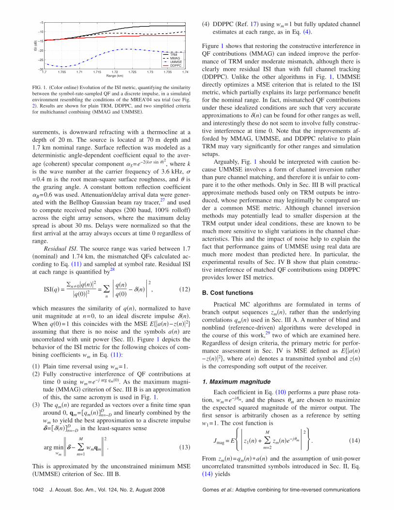
which measures the similarity of q�n�, normalized to haveunit magnitude at n=0, to an ideal discrete impulse ��n�.When q�0�=1 this coincides with the MSE E��a�n�−z�n��2�assuming that there is no noise and the symbols a�n� areuncorrelated with unit power �Sec. II�. Figure 1 depicts thebehavior of the ISI metric for the following choices of com-bining coefficients wm in Eq. �11�:

�1� Plain time reversal using wm=1.�2� Fully constructive interference of QF contributions at

time 0 using wm=e−j arg qm�0�. As the maximum magni-tude �MMAG� criterion of Sec. III B is an approximationof this, the same acronym is used in Fig. 1.

�3� The qm�n� are regarded as vectors over a finite time spanaround 0, qm= �qm�n��n=−D

D and linearly combined by thewm to yield the best approximation to a discrete impulse�= ��n��n=−D

D in the least-squares sense

arg minwm

� − �m=1

M

wmqm 2

. �13�

This is approximated by the unconstrained minimum MSE

1.7 1.705 1.71 1.715 1.72 1.725 1.73 1.735 1.74−30

−25

−20

−15

−10

−5

Range (km)

ISI(

dB)

TRMMMAGUMMSEDDPPC

FIG. 1. �Color online� Evolution of the ISI metric, quantifying the similaritybetween the symbol-rate-sampled QF and a discrete impulse, in a simulatedenvironment resembling the conditions of the MREA’04 sea trial �see Fig.2�. Results are shown for plain TRM, DDPPC, and two simplified criteriafor multichannel combining �MMAG and UMMSE�.

�UMMSE� criterion of Sec. III B.


�4� DDPPC �Ref. 17� using wm=1 but fully updated channelestimates at each range, as in Eq. �4�.

Figure 1 shows that restoring the constructive interference inQF contributions �MMAG� can indeed improve the perfor-mance of TRM under moderate mismatch, although there isclearly more residual ISI than with full channel tracking�DDPPC�. Unlike the other algorithms in Fig. 1, UMMSEdirectly optimizes a MSE criterion that is related to the ISImetric, which partially explains its large performance benefitfor the nominal range. In fact, mismatched QF contributionsunder these idealized conditions are such that very accurateapproximations to ��n� can be found for other ranges as well,and interestingly these do not seem to involve fully construc-tive interference at time 0. Note that the improvements af-forded by MMAG, UMMSE, and DDPPC relative to plainTRM may vary significantly for other ranges and simulationsetups.

Arguably, Fig. 1 should be interpreted with caution be-cause UMMSE involves a form of channel inversion ratherthan pure channel matching, and therefore it is unfair to com-pare it to the other methods. Only in Sec. III B will practicalapproximate methods based only on TRM outputs be intro-duced, whose performance may legitimally be compared un-der a common MSE metric. Although channel inversionmethods may potentially lead to smaller dispersion at theTRM output under ideal conditions, these are known to bemuch more sensitive to slight variations in the channel char-acteristics. This and the impact of noise help to explain thefact that performance gains of UMMSE using real data aremuch more modest than predicted here. In particular, theexperimental results of Sec. IV B show that plain construc-tive interference of matched QF contributions using DDPPCprovides lower ISI metrics.

B. Cost functions

Practical MC algorithms are formulated in terms ofbranch output sequences zm�n�, rather than the underlyingcorrelations qm�n� used in Sec. III A. A number of blind andnonblind �reference-driven� algorithms were developed inthe course of this work,29 two of which are examined here.Regardless of design criteria, the primary metric for perfor-mance assessment in Sec. IV is MSE defined as E��a�n�−z�n��2�, where a�n� denotes a transmitted symbol and z�n�is the corresponding soft output of the receiver.

1. Maximum magnitude

Each coefficient in Eq. �10� performs a pure phase rota-tion, wm=e−jm, and the phases m are chosen to maximizethe expected squared magnitude of the mirror output. Thefirst sensor is arbitrarily chosen as a reference by settingw1=1. The cost function is

Jmag = E��z1�n� + �m=2

M

zm�n�e−jm�2� . �14�

From zm�n�=qm�n��a�n� and the assumption of unit-poweruncorrelated transmitted symbols introduced in Sec. II, Eq.
�14� yields

Jmag = �n�q1�n� + �

m=2

M

qm�n�e−jm�2

. �15�

If the system operates with low mismatch, such that q�n��C��n� in Eq. �11�, then Eq. �15� will be largely dominatedby the contribution for n=0. Ignoring the remaining terms,an optimal solution for m is then readily given by m

=arg qm�0�−arg q1�0�.In Appendix B a simple adaptation rule for the angles

based on gradient ascent is derived by differentiating Eq.�14� with respect to m, obtaining a stochastic approximationto the gradient, and then using it as an error signal driving aphase-locked loop �PLL�-type filter.4 This yields

m�n + 1� = m�n� + K�m�n� , �16�

�m�n� = Im��z�n� − zm�n�e−jm�*zm�n�e−jm� , �17�

where the loop gain K is adjusted empirically. This adapta-tion rule does not require a reference signal and, as in mostblind filtering algorithms, a residual phase ambiguity existsthat manifests itself as a rotation of the signal constellation.Similar to plain TR, postprocessing is therefore needed toproperly align and scale the output constellation.

2. Unconstrained minimum MSE

Rather than aligning the zm with unit-magnitude rota-tions, arbitrary coefficients wm can be used to minimize theoutput error. In this work an exponentially weighted least-squares cost function is used,

Jumse�n� = �k=0

n

n−k�a�k� − �m=1

M

wm�n�zm�k��2

, �18�

so that time adaptation of the wm is actually carried out bythe RLS algorithm �Ref. 30�. Such a system effectively con-stitutes a very simple multichannel equalizer with one tap persensor, which exploits probe preprocessing to significantlyreduce the number of parameters to track. This approach willbe termed UMMSE as in Ref. 29 although, strictly speaking,Eq. �18� is not a statistical criterion but rather a deterministicone. In reference-driven filtering schemes the packet symbolsa�k� to be used in Eq. �18� are assumed known during aninitial training period, and afterward decisions based on thereceiver output are used �decision-directed mode�. Not onlydoes this method handle phase synchronization, it also elimi-nates the need for output normalization.

C. TRM postprocessing

Symbol synchronization. In a practical TRM the outputshould undergo symbol synchronization to determine thetime offset that maximizes a performance metric such as de-tection signal to noise ratio �SNR�. Because the Dopplercompensation technique of Sec. II A virtually eliminates anydiscrepancies in symbol rate, we simply calculate the Lpolyphase components of the oversampled discrete-time out-put, z�l��n��z��l+nL�Tb /L�, l=0, . . . ,L−1, and choose theone with strongest average power. This is unnecessary when
probes are estimated from data packets, as the best time off-

set is known to be zero beforehand because channel identi-fication removes delay ambiguities in pulse shapes.

Phase synchronization. Doppler compensation wasfound to be effective at eliminating carrier frequency mis-matches that result in sustained rotation of the TRM outputover time. Still, a popular PLL approach4 for phase synchro-nization was used as a postprocessor to track slow phasevariations and hence properly align the output constellation.Specifically, a loop filter similar to Eq. �16� is used to updatethe estimated phase , driven by the error signal ��n�=Im�a�n�*z�n�e−j�. Similar to Eq. �18�, local symbol deci-sions should be used for computing ��n� upon enteringdecision-directed mode after the packet preamble. To sim-plify the comparison between different algorithms for ISIcompensation �equalization, TRM, and multichannel com-bining�, the same reference-driven phase synchronizationmethod is used throughout this work. More appropriatechoices are available for carrier synchronization in practicalsystems when ISI mitigation does not rely on an externalreference.18

Output normalization. The final operation to be per-formed after symbol synchronization and constellation align-ment is to account for an unknown scaling introduced by thechannel and amplifiers at the transmitter and TRM. This gainvaries throughout data packets as the channel and QFchange, and should therefore be tracked by an automatic gaincontrol �AGC�-like system. A simple possibility is to recur-sively compute an exponentially weighted average of the un-normalized TRM magnitude

��n� = ��n − 1� + �1 − ��z�n��, 0 � � � 1, �19�

and for a unit-magnitude constellation generate the normal-ized output as z��n�=z�n��−1�n�. Strictly speaking, normal-ization is not required to slice M-PSK constellations, but it isuseful for estimating output MSE values.

IV. EXPERIMENTAL RESULTS

A. The MREA’04 experiment

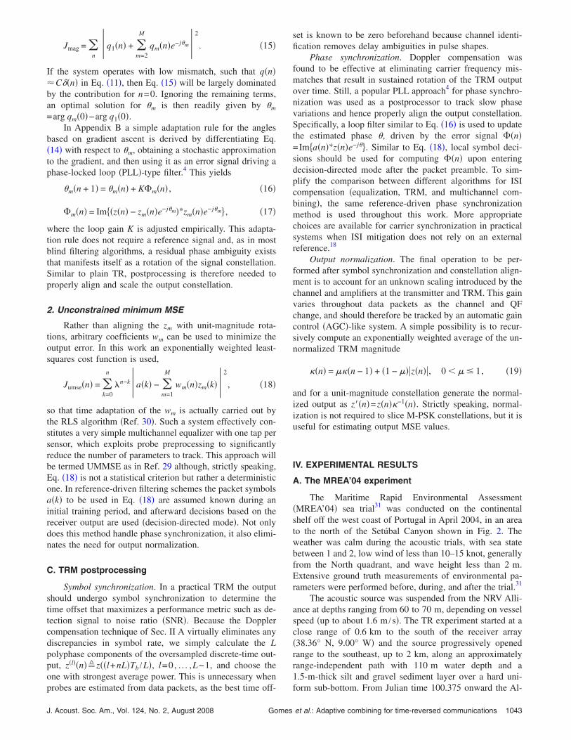
The Maritime Rapid Environmental Assessment�MREA’04� sea trial31 was conducted on the continentalshelf off the west coast of Portugal in April 2004, in an areato the north of the Setúbal Canyon shown in Fig. 2. Theweather was calm during the acoustic trials, with sea statebetween 1 and 2, low wind of less than 10–15 knot, generallyfrom the North quadrant, and wave height less than 2 m.Extensive ground truth measurements of environmental pa-rameters were performed before, during, and after the trial.31

The acoustic source was suspended from the NRV Alli-ance at depths ranging from 60 to 70 m, depending on vesselspeed �up to about 1.6 m /s�. The TR experiment started at aclose range of 0.6 km to the south of the receiver array�38.36° N, 9.00° W� and the source progressively openedrange to the southeast, up to 2 km, along an approximatelyrange-independent path with 110 m water depth and a1.5-m-thick silt and gravel sediment layer over a hard uni-
form sub-bottom. From Julian time 100.375 onward the Al-

liance maneuvered around a fixed position. The sound-speedprofile was downward refracting, with a thermocline at adepth of about 20 m.

The drifting receiver is an acoustic oceanographic buoy�AOB� developed at the University of Algarve. The AOB candigitize and record eight hydrophone signals in the frequencyband �0.1,16� kHz, sampled at up to 60 kHz. A wireless link�WLAN� provides remote access to status information anddata snapshots at ranges up to 10–20 km. In addition to eighthydrophones, vertically placed at depths 10, 15, 55, 60, 65,70, 75, and 80 m, the AOB also has a 16-sensor thermistorchain spanning 80 m for water column temperature monitor-ing.

During a period of approximately 90 min modulateddata were transmitted at a carrier frequency of 3.6 kHz, us-ing symbol rates of 200 or 400 baud, and both 2-PSK and4-PSK constellations. As discussed in Sec. II, fourth-rootraised-cosine signaling pulses with 100% rolloff were usedto simplify out-of-band noise removal at the receiver bymatched filtering to the transmitted pulse shape. The signalbandwidth is therefore 400 Hz at 200 baud and is 800 Hz at400 baud. Each individual transmission comprises a singletruncated signaling pulse �ping� acting as a channel probewith symmetrical guard intervals for a total duration of 1 s,followed by a 20 s data packet. To enhance the SNR whendirectly measuring channel responses, probe pulses were sentwith double the amplitude of signaling pulses in data pack-ets. The source sequentially transmitted four packets for eachof the following modulation formats: 2-PSK/ 200 baud,2-PSK/ 400 baud, 4-PSK/ 200 baud, and 4-PSK/ 400 baud.The whole activity cycle, lasting for 336 s, was repeated ev-ery 360 s. The data set analyzed here comprises 200 probe/

(m)

FIG. 2. �Color online� Site map for the MREA’04 sea trial, conducted offthe west coast of Portugal in April 2004. The TR experiment took place inan approximately range-independent area �38.36°N, 9.00°W� with 110 mdepth and downward-refracting sound-speed profile. The drifting receiverarray had eight hydrophones at depths 10, 15, 55, 60, 65, 70, 75, and 80 m.The acoustic source was suspended from the NRV Alliance at depths of60–70 m and towed at up to 1.6 m /s. Throughout the experiment thesource-array range varied from 0.6 to 2 km.

packet pairs.


B. Performance analysis

Received signals were passband filtered, sampled at20 080 Hz, and converted to baseband. Packets were classi-fied and frame synchronized by crosscorrelation with the first2 kilosamples of all known modulated wave forms, thenmatch filtered by the appropriate fourth-root raised-cosinepulse and resampled �oversampled� at L=4 times the symbolrate. No attempt was made to detect the channel probes; theywere segmented based on their known position relative to thebeginning of data packets, then match filtered and resampledas above.

1. Notes on filtering

Throughout Sec. IV B �m ,n� will denote the length of asingle-channel filter with m causal coefficients and n anti-causal ones. A multiple-input/single-output filter comprisingp single-channel parallel filters of length �m ,n� whose out-puts are added to create a scalar output will be denoted by�m ,n�� p. Such p-channel filters are used when processingfractionally sampled communications wave forms and/ormultisensor data, such that p equals the oversampling factor�relative to the symbol rate� times the number of sensors. Inpractical reference-driven filtering schemes, n anticausal co-efficients are effectively obtained when the reference signalis delayed by n samples with respect to the received signals.In non-reference-driven �blind� schemes the distinction be-tween causal and anticausal coefficients is meaningless and�m ,n� should simply be interpreted as a filter with m+n co-efficients.

Regarding equalization, choosing a good combination offilter lengths from channel estimates under fractional sam-pling is known to be unreliable and often done offline by trialand error. For decision-feedback equalizers �DFEs� populardesign guidelines32 recommend using the feedback filter tocancel causal �postcursor� ISI, whereas feedforward filterswill be much shorter to capture multipath energy and cancelanticausal �precursor� ISI. In this work appropriate equalizerlengths were set empirically for each packet in each experi-ment by searching over a plausible range of candidatelengths and selecting the one yielding the best performance.Somewhat unexpectedly, the best lengths reported belowwere found to be consistent across a clear majority of both200 and 400 baud packets.

As in other references,33 the impact of symbol errors onthe performance of reference-driven channel estimation,equalization, and phase tracking algorithms is not addressedin this work. These subsystems are always operated in train-ing mode, where the correct symbols are known, and thecalculated performance metrics should then be interpreted asoptimistic estimates of what could actually be achieved. Forvalues of output MSE higher than about −5 dB the numberof symbol errors is sufficiently large to have a significantimpact on performance in decision-directed mode. Thismight cause divergence of adaptive algorithms if correctivemeasures are not implemented, such as freezing the updating
of coefficients when unreliable decisions are detected.

2. Channel responses

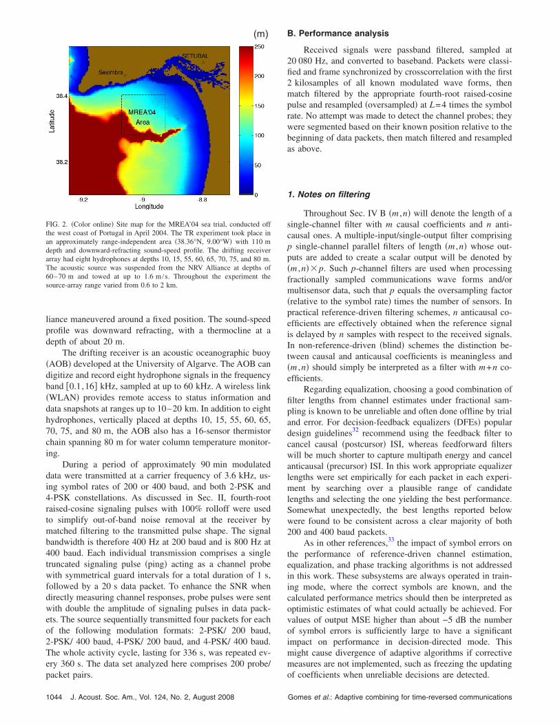
Figure 3�a� shows the evolution of the estimated impulseresponse at depth 75 m in one of the received 400 baudpackets �PKT 149� with significant Doppler distortion. Chan-nel identification was performed independently for each sen-sor using the exponentially windowed RLS algorithm.30 Forcomputational efficiency, each L-oversampled hydrophonesignal was split into L polyphase components, ym

�l��n�=ym�l+nL�, and these were used as references to a bank of Lparallel RLS transversal filters fed by the known packet sym-bols. Each filter operates with 41 causal and 10 anticausalcoefficients �abbreviated as �41,10� using the notation intro-duced in Sec. IV B 1� and forgetting factor =0.95 empiri-cally adjusted to minimize the residual error variance. Thistechnique decreases the overall computational complexity bya factor of L relative to direct identification of ym�n� from thezero-interpolated symbol sequence. Snapshots of the RLScoefficient vectors �estimated polyphase components of im-pulse responses� were taken every 20 symbol intervals andrearranged in the correct temporal order to produce the plot.The multipath arrival structure, spanning about 50 ms, is rea-sonably sparse and clearly visible in Fig. 3�a�, as well as atime compression due to Doppler that causes the arrivals toslip by 14 samples �3.5 symbols� in the course of a 20 spacket. Figure 3�b� shows the impulse response estimate forthe same packet after Doppler compensation as described inSec. II A and Appendix A, where the multipath structure isseen to remain essentially unaltered. The coherence time forthe channel of Fig. 3�b� was estimated to be about 1 s �Dop-

(a)

(b)

FIG. 3. �Color online� Evolution of amplitude-normalized estimated channelresponses at depth 75 m �hydrophone 7� for packet 149 �400 baud�. A hori-zontal slice through any of the plots represents a snapshot of the time-varying response. The coherence time for this channel was estimated to beabout 1 s. Estimates are based on RLS transversal filtering, four-oversampling, filter order �41, 10� per polyphase component �for order no-tation see Sec. IV B 1�, and =0.95. �a� Before Doppler compensation, fd

=1.65 Hz at the carrier frequency of 3.6 kHz. �b� After broadband Dopplercompensation as described in Sec. II A.

pler bandwidth of 1 Hz�. Once the average Doppler scaling


in received signals was compensated, it was found that in-cluding other dedicated symbol synchronization subsystemsat the receiver was unnecessary. The various structures de-scribed below use fractional sampling, which can automati-cally perform fine adjustments to the sampling instants whenneeded.

The causal/anticausal filter lengths used in Fig. 3 wereempirically chosen to capture most of the multipath energyin all 400 baud packets of the data set. In 200 baud packetsthe filter lengths used for channel identification could be re-duced to �21, 7� without significantly affecting the residualerror, i.e., while still capturing all relevant multipaths.

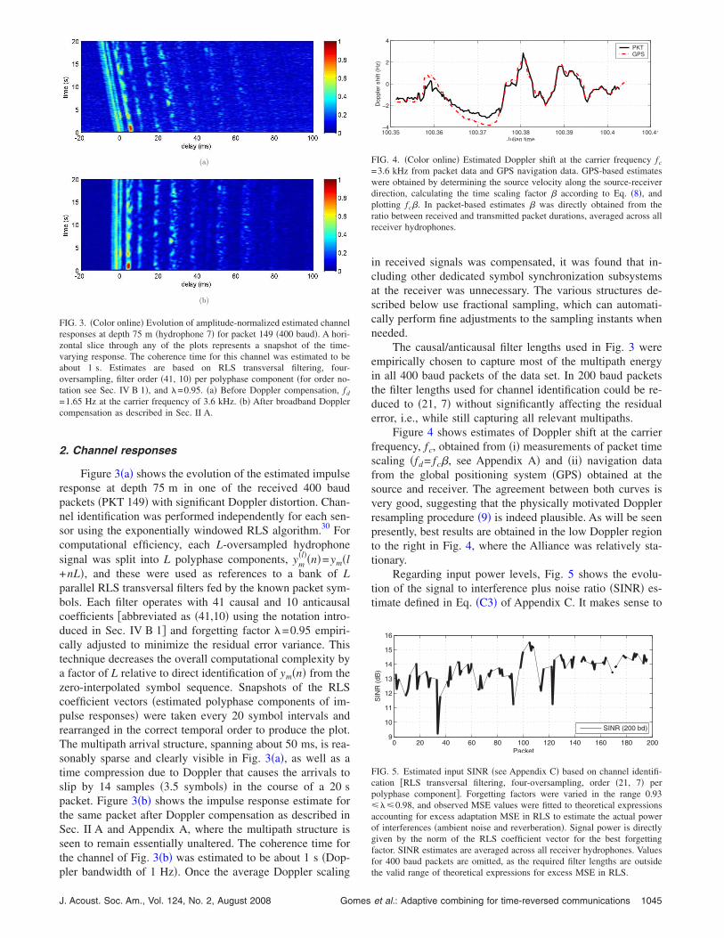
Figure 4 shows estimates of Doppler shift at the carrierfrequency, fc, obtained from �i� measurements of packet timescaling �fd= fc�, see Appendix A� and �ii� navigation datafrom the global positioning system �GPS� obtained at thesource and receiver. The agreement between both curves isvery good, suggesting that the physically motivated Dopplerresampling procedure �9� is indeed plausible. As will be seenpresently, best results are obtained in the low Doppler regionto the right in Fig. 4, where the Alliance was relatively sta-tionary.

Regarding input power levels, Fig. 5 shows the evolu-tion of the signal to interference plus noise ratio �SINR� es-timate defined in Eq. �C3� of Appendix C. It makes sense to

100.35 100.36 100.37 100.38 100.39 100.4 100.41−4

−2

0

2

4

Julian time

Dopplershift(Hz)

PKTGPS

FIG. 4. �Color online� Estimated Doppler shift at the carrier frequency fc

=3.6 kHz from packet data and GPS navigation data. GPS-based estimateswere obtained by determining the source velocity along the source-receiverdirection, calculating the time scaling factor � according to Eq. �8�, andplotting fc�. In packet-based estimates � was directly obtained from theratio between received and transmitted packet durations, averaged across allreceiver hydrophones.

0 20 40 60 80 100 120 140 160 180 2009

10

11

12

13

14

15

16

Packet

SIN

R(d

B)

SINR (200 bd)

FIG. 5. Estimated input SINR �see Appendix C� based on channel identifi-cation �RLS transversal filtering, four-oversampling, order �21, 7� perpolyphase component�. Forgetting factors were varied in the range 0.93� �0.98, and observed MSE values were fitted to theoretical expressionsaccounting for excess adaptation MSE in RLS to estimate the actual powerof interferences �ambient noise and reverberation�. Signal power is directlygiven by the norm of the RLS coefficient vector for the best forgettingfactor. SINR estimates are averaged across all receiver hydrophones. Valuesfor 400 baud packets are omitted, as the required filter lengths are outside
the valid range of theoretical expressions for excess MSE in RLS.

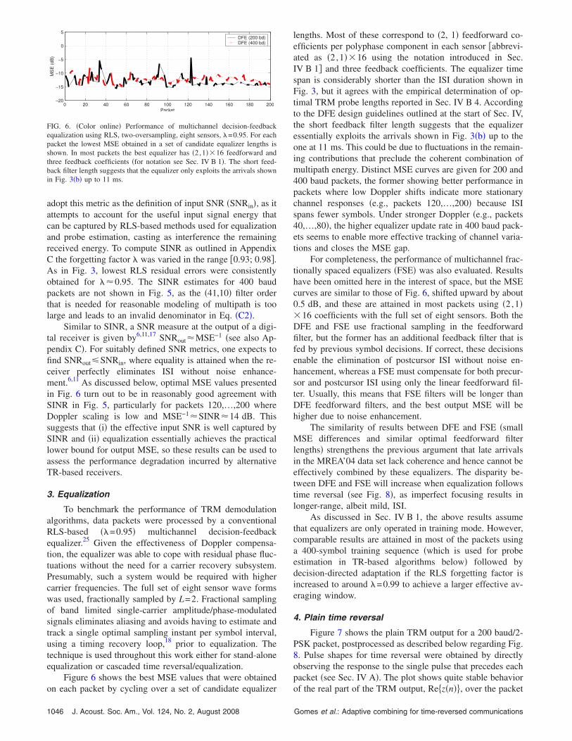
adopt this metric as the definition of input SNR �SNRin�, as itattempts to account for the useful input signal energy thatcan be captured by RLS-based methods used for equalizationand probe estimation, casting as interference the remainingreceived energy. To compute SINR as outlined in AppendixC the forgetting factor was varied in the range �0.93; 0.98�.As in Fig. 3, lowest RLS residual errors were consistentlyobtained for �0.95. The SINR estimates for 400 baudpackets are not shown in Fig. 5, as the �41,10� filter orderthat is needed for reasonable modeling of multipath is toolarge and leads to an invalid denominator in Eq. �C2�.

Similar to SINR, a SNR measure at the output of a digi-tal receiver is given by6,11,17 SNRout�MSE−1 �see also Ap-pendix C�. For suitably defined SNR metrics, one expects tofind SNRout�SNRin, where equality is attained when the re-ceiver perfectly eliminates ISI without noise enhance-ment.6,11 As discussed below, optimal MSE values presentedin Fig. 6 turn out to be in reasonably good agreement withSINR in Fig. 5, particularly for packets 120,…,200 whereDoppler scaling is low and MSE−1�SINR�14 dB. Thissuggests that �i� the effective input SNR is well captured bySINR and �ii� equalization essentially achieves the practicallower bound for output MSE, so these results can be used toassess the performance degradation incurred by alternativeTR-based receivers.

3. Equalization

To benchmark the performance of TRM demodulationalgorithms, data packets were processed by a conventionalRLS-based � =0.95� multichannel decision-feedbackequalizer.25 Given the effectiveness of Doppler compensa-tion, the equalizer was able to cope with residual phase fluc-tuations without the need for a carrier recovery subsystem.Presumably, such a system would be required with highercarrier frequencies. The full set of eight sensor wave formswas used, fractionally sampled by L=2. Fractional samplingof band limited single-carrier amplitude/phase-modulatedsignals eliminates aliasing and avoids having to estimate andtrack a single optimal sampling instant per symbol interval,using a timing recovery loop,18 prior to equalization. Thetechnique is used throughout this work either for stand-aloneequalization or cascaded time reversal/equalization.

Figure 6 shows the best MSE values that were obtained

0 20 40 60 80 100 120 140 160 180 200−20

−15

−10

−5

0

5

Packet

MSE(dB)

DFE (200 bd)DFE (400 bd)

FIG. 6. �Color online� Performance of multichannel decision-feedbackequalization using RLS, two-oversampling, eight sensors, =0.95. For eachpacket the lowest MSE obtained in a set of candidate equalizer lengths isshown. In most packets the best equalizer has �2,1��16 feedforward andthree feedback coefficients �for notation see Sec. IV B 1�. The short feed-back filter length suggests that the equalizer only exploits the arrivals shownin Fig. 3�b� up to 11 ms.

on each packet by cycling over a set of candidate equalizer


lengths. Most of these correspond to �2, 1� feedforward co-efficients per polyphase component in each sensor �abbrevi-ated as �2,1��16 using the notation introduced in Sec.IV B 1� and three feedback coefficients. The equalizer timespan is considerably shorter than the ISI duration shown inFig. 3, but it agrees with the empirical determination of op-timal TRM probe lengths reported in Sec. IV B 4. Accordingto the DFE design guidelines outlined at the start of Sec. IV,the short feedback filter length suggests that the equalizeressentially exploits the arrivals shown in Fig. 3�b� up to theone at 11 ms. This could be due to fluctuations in the remain-ing contributions that preclude the coherent combination ofmultipath energy. Distinct MSE curves are given for 200 and400 baud packets, the former showing better performance inpackets where low Doppler shifts indicate more stationarychannel responses �e.g., packets 120,…,200� because ISIspans fewer symbols. Under stronger Doppler �e.g., packets40,…,80�, the higher equalizer update rate in 400 baud pack-ets seems to enable more effective tracking of channel varia-tions and closes the MSE gap.

For completeness, the performance of multichannel frac-tionally spaced equalizers �FSE� was also evaluated. Resultshave been omitted here in the interest of space, but the MSEcurves are similar to those of Fig. 6, shifted upward by about0.5 dB, and these are attained in most packets using �2,1��16 coefficients with the full set of eight sensors. Both theDFE and FSE use fractional sampling in the feedforwardfilter, but the former has an additional feedback filter that isfed by previous symbol decisions. If correct, these decisionsenable the elimination of postcursor ISI without noise en-hancement, whereas a FSE must compensate for both precur-sor and postcursor ISI using only the linear feedforward fil-ter. Usually, this means that FSE filters will be longer thanDFE feedforward filters, and the best output MSE will behigher due to noise enhancement.

The similarity of results between DFE and FSE �smallMSE differences and similar optimal feedforward filterlengths� strengthens the previous argument that late arrivalsin the MREA’04 data set lack coherence and hence cannot beeffectively combined by these equalizers. The disparity be-tween DFE and FSE will increase when equalization followstime reversal �see Fig. 8�, as imperfect focusing results inlonger-range, albeit mild, ISI.

As discussed in Sec. IV B 1, the above results assumethat equalizers are only operated in training mode. However,comparable results are attained in most of the packets usinga 400-symbol training sequence �which is used for probeestimation in TR-based algorithms below� followed bydecision-directed adaptation if the RLS forgetting factor isincreased to around =0.99 to achieve a larger effective av-eraging window.

4. Plain time reversal

Figure 7 shows the plain TRM output for a 200 baud/2-PSK packet, postprocessed as described below regarding Fig.8. Pulse shapes for time reversal were obtained by directlyobserving the response to the single pulse that precedes eachpacket �see Sec. IV A�. The plot shows quite stable behavior
of the real part of the TRM output, Re�z�n��, over the packet

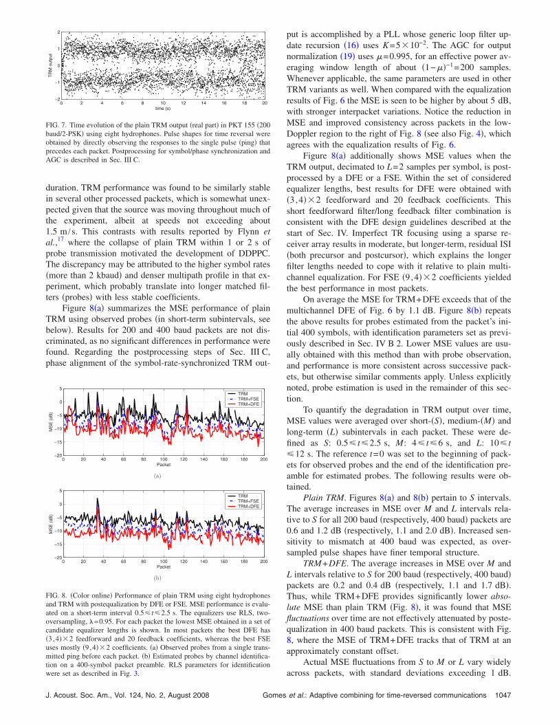
duration. TRM performance was found to be similarly stablein several other processed packets, which is somewhat unex-pected given that the source was moving throughout much ofthe experiment, albeit at speeds not exceeding about1.5 m /s. This contrasts with results reported by Flynn etal.,17 where the collapse of plain TRM within 1 or 2 s ofprobe transmission motivated the development of DDPPC.The discrepancy may be attributed to the higher symbol rates�more than 2 kbaud� and denser multipath profile in that ex-periment, which probably translate into longer matched fil-ters �probes� with less stable coefficients.

Figure 8�a� summarizes the MSE performance of plainTRM using observed probes �in short-term subintervals, seebelow�. Results for 200 and 400 baud packets are not dis-criminated, as no significant differences in performance werefound. Regarding the postprocessing steps of Sec. III C,phase alignment of the symbol-rate-synchronized TRM out-

0 2 4 6 8 10 12 14 16 18 20−2

−1

0

1

2

time (s)

TR

Mou

tput

FIG. 7. Time evolution of the plain TRM output �real part� in PKT 155 �200baud/2-PSK� using eight hydrophones. Pulse shapes for time reversal wereobtained by directly observing the responses to the single pulse �ping� thatprecedes each packet. Postprocessing for symbol/phase synchronization andAGC is described in Sec. III C.

0 20 40 60 80 100 120 140 160 180 200−20

−15

−10

−5

0

5

Packet

MS

E(d

B)

TRMTRM+FSETRM+DFE

(a)

0 20 40 60 80 100 120 140 160 180 200−20

−15

−10

−5

0

5

Packet

MS

E(d

B)

TRMTRM+FSETRM+DFE

(b)

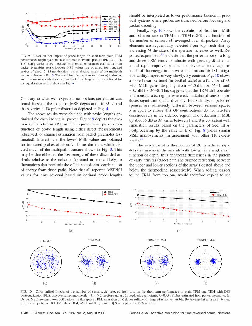
FIG. 8. �Color online� Performance of plain TRM using eight hydrophonesand TRM with postequalization by DFE or FSE. MSE performance is evalu-ated on a short-term interval 0.5� t�2.5 s. The equalizers use RLS, two-oversampling, =0.95. For each packet the lowest MSE obtained in a set ofcandidate equalizer lengths is shown. In most packets the best DFE has�3,4��2 feedforward and 20 feedback coefficients, whereas the best FSEuses mostly �9,4��2 coefficients. �a� Observed probes from a single trans-mitted ping before each packet. �b� Estimated probes by channel identifica-tion on a 400-symbol packet preamble. RLS parameters for identification
were set as described in Fig. 3.

put is accomplished by a PLL whose generic loop filter up-date recursion �16� uses K=5�10−2. The AGC for outputnormalization �19� uses �=0.995, for an effective power av-eraging window length of about �1−��−1=200 samples.Whenever applicable, the same parameters are used in otherTRM variants as well. When compared with the equalizationresults of Fig. 6 the MSE is seen to be higher by about 5 dB,with stronger interpacket variations. Notice the reduction inMSE and improved consistency across packets in the low-Doppler region to the right of Fig. 8 �see also Fig. 4�, whichagrees with the equalization results of Fig. 6.

Figure 8�a� additionally shows MSE values when theTRM output, decimated to L=2 samples per symbol, is post-processed by a DFE or a FSE. Within the set of consideredequalizer lengths, best results for DFE were obtained with�3,4��2 feedforward and 20 feedback coefficients. Thisshort feedforward filter/long feedback filter combination isconsistent with the DFE design guidelines described at thestart of Sec. IV. Imperfect TR focusing using a sparse re-ceiver array results in moderate, but longer-term, residual ISI�both precursor and postcursor�, which explains the longerfilter lengths needed to cope with it relative to plain multi-channel equalization. For FSE �9,4��2 coefficients yieldedthe best performance in most packets.

On average the MSE for TRM+DFE exceeds that of themultichannel DFE of Fig. 6 by 1.1 dB. Figure 8�b� repeatsthe above results for probes estimated from the packet’s ini-tial 400 symbols, with identification parameters set as previ-ously described in Sec. IV B 2. Lower MSE values are usu-ally obtained with this method than with probe observation,and performance is more consistent across successive pack-ets, but otherwise similar comments apply. Unless explicitlynoted, probe estimation is used in the remainder of this sec-tion.

To quantify the degradation in TRM output over time,MSE values were averaged over short-�S�, medium-�M� andlong-term �L� subintervals in each packet. These were de-fined as S: 0.5� t�2.5 s, M: 4� t�6 s, and L: 10� t�12 s. The reference t=0 was set to the beginning of pack-ets for observed probes and the end of the identification pre-amble for estimated probes. The following results were ob-tained.

Plain TRM. Figures 8�a� and 8�b� pertain to S intervals.The average increases in MSE over M and L intervals rela-tive to S for all 200 baud �respectively, 400 baud� packets are0.6 and 1.2 dB �respectively, 1.1 and 2.0 dB�. Increased sen-sitivity to mismatch at 400 baud was expected, as over-sampled pulse shapes have finer temporal structure.

TRM+DFE. The average increases in MSE over M andL intervals relative to S for 200 baud �respectively, 400 baud�packets are 0.2 and 0.4 dB �respectively, 1.1 and 1.7 dB�.Thus, while TRM+DFE provides significantly lower abso-lute MSE than plain TRM �Fig. 8�, it was found that MSEfluctuations over time are not effectively attenuated by poste-qualization in 400 baud packets. This is consistent with Fig.8, where the MSE of TRM+DFE tracks that of TRM at anapproximately constant offset.

Actual MSE fluctuations from S to M or L vary widely
across packets, with standard deviations exceeding 1 dB.

Contrary to what was expected, no obvious correlation wasfound between the extent of MSE degradation in M, L andthe severity of Doppler distortion depicted in Fig. 4.

The above results were obtained with probe lengths op-timized for each individual packet. Figure 9 depicts the evo-lution of short-term MSE in three representative packets as afunction of probe length using either direct measurements�observed� or channel estimation from packet preambles �es-timated�. Interestingly, the lowest MSE values are obtainedfor truncated probes of about 7–15 ms duration, which dis-card much of the multipath structure shown in Fig. 3. Thismay be due either to the low energy of these discarded ar-rivals relative to the noise background or, more likely, tofluctuations that preclude the effective coherent combinationof energy from those paths. Note that all reported MSE/ISIvalues for time reversal based on optimal probe lengths

0 5 10 15 20 25 30 35 40 45 50−8

−6

−4

−2

0

Probe length (ms)

MSE(dB)

#30 obs.

#30 est.

#104 obs.

#104 est.

#113 obs.

#113 est.

FIG. 9. �Color online� Impact of probe length on short-term plain TRMperformance �eight hydrophones� for three individual packets �PKT 30, 104,113� using direct probe measurements �obs.� or channel estimation frompacket preambles �est.�. Lowest MSE values are obtained for truncatedprobes of about 7–15 ms duration, which discard much of the multipathstructure shown in Fig. 3. The trend for other packets �not shown� is similar,and in agreement with the short feedback filter lengths that were found forthe equalization results shown in Fig. 6.

1 2 3 4 5 6 7 8−14

−12

−10

−8

−6

−4

−2

0

Number of receivers

MS

E(d

B)

TRMTRM+DFE

(a)

��

(c)

��

(d)

FIG. 10. �Color online� Impact of the number of sensors, M, selected fpostequalization �RLS, two-oversampling, �mostly� �3,4��2 feedforward anOutput MSE, averaged over 200 packets. In this sparse TRM, saturation of M
�d�� Scatter plots for PKT 155, plain TRM, M =1 and 8. ��e� and �f�� Scatter plo

should be interpreted as lower performance bounds in prac-tical systems where probes are truncated before focusing andpacket decoding.

Finally, Fig. 10 shows the evolution of short-term MSEand bit error rate in TRM and TRM+DFE as a function ofthe number of sensors M, averaged over all packets. Arrayelements are sequentially selected from top, such that byincreasing M the size of the aperture increases as well. Re-ported experiments11 indicate that the performance of a longand dense TRM tends to saturate with growing M after aninitial rapid improvement, as the device already capturesmuch of the energy in the water column and its ISI mitiga-tion ability improves very slowly. By contrast, Fig. 10 showsa more linearlike trend �in decibel scale� as a function of M,with MSE gains dropping from −1.5 dB for M =2 until−0.7 dB for M =8. This suggests that the TRM still operatesin a nonsaturated regime where each additional sensor intro-duces significant spatial diversity. Equivalently, impulse re-sponses are sufficiently different between sensors spaced5 m apart to ensure that QF contributions do not interfereconstructively in the sidelobe region. The reduction in MSEby about 6 dB as M varies between 1 and 8 is consistent withsimulation results based on the parameters of Sec. III A.Postprocessing by the same DFE of Fig. 8 yields similarMSE improvements, in agreement with other TR experi-ments.11

The existence of a thermocline at 20 m induces rapiddelay variations in the arrivals with low grazing angles as afunction of depth, thus enhancing differences in the patternof early arrivals �direct path and surface reflection� betweenthe upper and lower sections of the array �located above andbelow the thermocline, respectively�. When adding sensorsto the TRM from top one would therefore expect to see

� � � � � � � ��

��

��

��

��

�

��

��

��

��

(b)

��

(e)

��

(f)

top, on the short-term performance of plain TRM and TRM with DFEfeedback coefficients, =0.95�. Probes estimated from packet preambles. �a�for sufficiently large M is not yet visible. �b� Average bit error rate. ��c� and

romd 20

SE
ts for TRM+DFE.

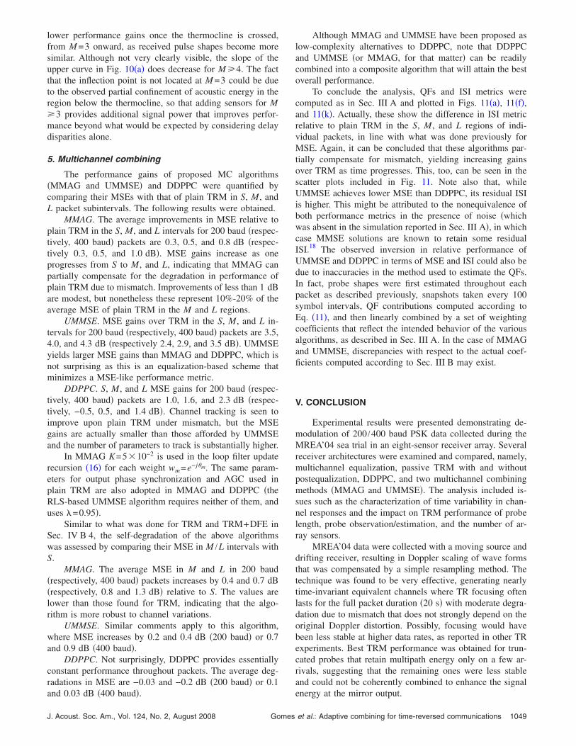
lower performance gains once the thermocline is crossed,from M =3 onward, as received pulse shapes become moresimilar. Although not very clearly visible, the slope of theupper curve in Fig. 10�a� does decrease for M �4. The factthat the inflection point is not located at M =3 could be dueto the observed partial confinement of acoustic energy in theregion below the thermocline, so that adding sensors for M�3 provides additional signal power that improves perfor-mance beyond what would be expected by considering delaydisparities alone.

5. Multichannel combining

The performance gains of proposed MC algorithms�MMAG and UMMSE� and DDPPC were quantified bycomparing their MSEs with that of plain TRM in S, M, andL packet subintervals. The following results were obtained.

MMAG. The average improvements in MSE relative toplain TRM in the S, M, and L intervals for 200 baud �respec-tively, 400 baud� packets are 0.3, 0.5, and 0.8 dB �respec-tively 0.3, 0.5, and 1.0 dB�. MSE gains increase as oneprogresses from S to M, and L, indicating that MMAG canpartially compensate for the degradation in performance ofplain TRM due to mismatch. Improvements of less than 1 dBare modest, but nonetheless these represent 10%-20% of theaverage MSE of plain TRM in the M and L regions.

UMMSE. MSE gains over TRM in the S, M, and L in-tervals for 200 baud �respectively, 400 baud� packets are 3.5,4.0, and 4.3 dB �respectively 2.4, 2.9, and 3.5 dB�. UMMSEyields larger MSE gains than MMAG and DDPPC, which isnot surprising as this is an equalization-based scheme thatminimizes a MSE-like performance metric.

DDPPC. S, M, and L MSE gains for 200 baud �respec-tively, 400 baud� packets are 1.0, 1.6, and 2.3 dB �respec-tively, −0.5, 0.5, and 1.4 dB�. Channel tracking is seen toimprove upon plain TRM under mismatch, but the MSEgains are actually smaller than those afforded by UMMSEand the number of parameters to track is substantially higher.

In MMAG K=5�10−2 is used in the loop filter updaterecursion �16� for each weight wm=e−jm. The same param-eters for output phase synchronization and AGC used inplain TRM are also adopted in MMAG and DDPPC �theRLS-based UMMSE algorithm requires neither of them, anduses =0.95�.

Similar to what was done for TRM and TRM+DFE inSec. IV B 4, the self-degradation of the above algorithmswas assessed by comparing their MSE in M /L intervals withS.

MMAG. The average MSE in M and L in 200 baud�respectively, 400 baud� packets increases by 0.4 and 0.7 dB�respectively, 0.8 and 1.3 dB� relative to S. The values arelower than those found for TRM, indicating that the algo-rithm is more robust to channel variations.

UMMSE. Similar comments apply to this algorithm,where MSE increases by 0.2 and 0.4 dB �200 baud� or 0.7and 0.9 dB �400 baud�.

DDPPC. Not surprisingly, DDPPC provides essentiallyconstant performance throughout packets. The average deg-radations in MSE are −0.03 and −0.2 dB �200 baud� or 0.1
and 0.03 dB �400 baud�.

Although MMAG and UMMSE have been proposed aslow-complexity alternatives to DDPPC, note that DDPPCand UMMSE �or MMAG, for that matter� can be readilycombined into a composite algorithm that will attain the bestoverall performance.

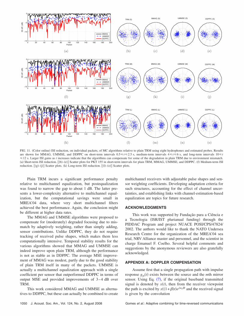
To conclude the analysis, QFs and ISI metrics werecomputed as in Sec. III A and plotted in Figs. 11�a�, 11�f�,and 11�k�. Actually, these show the difference in ISI metricrelative to plain TRM in the S, M, and L regions of indi-vidual packets, in line with what was done previously forMSE. Again, it can be concluded that these algorithms par-tially compensate for mismatch, yielding increasing gainsover TRM as time progresses. This, too, can be seen in thescatter plots included in Fig. 11. Note also that, whileUMMSE achieves lower MSE than DDPPC, its residual ISIis higher. This might be attributed to the nonequivalence ofboth performance metrics in the presence of noise �whichwas absent in the simulation reported in Sec. III A�, in whichcase MMSE solutions are known to retain some residualISI.18 The observed inversion in relative performance ofUMMSE and DDPPC in terms of MSE and ISI could also bedue to inaccuracies in the method used to estimate the QFs.In fact, probe shapes were first estimated throughout eachpacket as described previously, snapshots taken every 100symbol intervals, QF contributions computed according toEq. �11�, and then linearly combined by a set of weightingcoefficients that reflect the intended behavior of the variousalgorithms, as described in Sec. III A. In the case of MMAGand UMMSE, discrepancies with respect to the actual coef-ficients computed according to Sec. III B may exist.

V. CONCLUSION

Experimental results were presented demonstrating de-modulation of 200 /400 baud PSK data collected during theMREA’04 sea trial in an eight-sensor receiver array. Severalreceiver architectures were examined and compared, namely,multichannel equalization, passive TRM with and withoutpostequalization, DDPPC, and two multichannel combiningmethods �MMAG and UMMSE�. The analysis included is-sues such as the characterization of time variability in chan-nel responses and the impact on TRM performance of probelength, probe observation/estimation, and the number of ar-ray sensors.

MREA’04 data were collected with a moving source anddrifting receiver, resulting in Doppler scaling of wave formsthat was compensated by a simple resampling method. Thetechnique was found to be very effective, generating nearlytime-invariant equivalent channels where TR focusing oftenlasts for the full packet duration �20 s� with moderate degra-dation due to mismatch that does not strongly depend on theoriginal Doppler distortion. Possibly, focusing would havebeen less stable at higher data rates, as reported in other TRexperiments. Best TRM performance was obtained for trun-cated probes that retain multipath energy only on a few ar-rivals, suggesting that the remaining ones were less stableand could not be coherently combined to enhance the signal
energy at the mirror output.

Plain TRM incurs a significant performance penaltyrelative to multichannel equalization, but postequalizationwas found to narrow the gap to about 1 dB. The latter pre-sents a lower-complexity alternative to multichannel equal-ization, but the computational savings were small inMREA’04 data, where very short multichannel filtersachieved the best performance. Again, the conclusion mightbe different at higher data rates.

The MMAG and UMMSE algorithms were proposed tocompensate for �moderately� degraded focusing due to mis-match by adaptively weighting, rather than simply adding,sensor contributions. Unlike DDPPC, they do not requiretracking of received pulse shapes, which makes them lesscomputationally intensive. Temporal stability results for thevarious algorithms showed that MMAG and UMMSE canindeed improve upon plain TRM, although the performanceis not as stable as in DDPPC. The average MSE improve-ment of MMAG was modest, partly due to the good stabilityof plain TRM itself in many of the packets. UMMSE isactually a multichannel equalization approach with a singlecoefficient per sensor that outperformed DDPPC in terms ofoutput MSE and provided improvements of 3–4 dB overTRM.

This work considered MMAG and UMMSE as alterna-

� ��

��

��

�

��

��

��

��

��

(a)

� ��

��

��

�

��

��

��

��

��

(f)

� ��

��

��

�

��

��

��

��

��

(k)

FIG. 11. �Color online� ISI reduction, on individual packets, of MC algorithare shown for MMAG, UMMSE, and DDPPC on short-term intervals 0.�12 s. Larger ISI gains as t increases indicate that the algorithms can comp�a� Short-term ISI reduction. ��b�–�e�� Scatter plots for PKT 155 in short-termreduction. ��g�–�j�� Scatter plots. �k� Long-term ISI reduction. ��l�–�o�� Scat

tives to DDPPC, but these can actually be combined to create


multichannel receivers with adjustable pulse shapes and sen-sor weighting coefficients. Developing adaptation criteria forsuch structures, accounting for the effect of channel uncer-tainties, and establishing links with channel-estimation-basedequalization are topics for future research.

ACKNOWLEDGMENTS

This work was supported by Fundação para a Ciência ea Tecnologia �ISR/IST plurianual funding� through thePIDDAC Program and project NUACE POSI/CPS/47824/2002. The authors would like to thank the NATO UnderseaResearch Centre for the organization of the MREA’04 seatrial, NRV Alliance master and personnel, and the scientist incharge Emanuel F. Coelho. Several helpful comments andsuggestions by the anonymous reviewers are also gratefullyacknowledged.

APPENDIX A: DOPPLER COMPENSATION

Assume first that a single propagation path with impulseresponse gm�t� exists between the source and the mth mirrorsensor. Using Eq. �7�, if the original baseband transmittedsignal is denoted by x�t�, then from the receiver viewpointthe path is excited by x��1+��t�ej�c�t and the received signal

TRM (S)

(b)

MMAG (S)

(c)

UMMSE (S)

(d)

DDPPC (S)

(e)

RM (M)

(g)

MMAG (M)

(h)

UMMSE (M)

(i)

DDPPC (M)

(j)

TRM (L)

(l)

MMAG (L)

(m)

UMMSE (L)

(n)

DDPPC (L)

(o)

lative to plain TRM using eight hydrophones and estimated probes. Results2.5 s, medium-term intervals 4� t�6 s, and long-term intervals 10� t

e for some of the degradation in plain TRM due to environment mismatch.rvals for plain TRM, MMAG, UMMSE, and DDPPC. �f� Medium-term ISIots.

T

ms re5� t�ensat

inteter pl

is given by the convolution


ym�t� =� x��1 + ��t − ��ej�c��t−��gm��d�

=� x�t − ��ej��c�/�1+��t−��

1 + �gm �� + �t

1 + �d��.

�A1�

This is recognized as a linear convolution between x�t� and atime-varying impulse response whose magnitude equals�gm�� for ��1, with the origin shifted to −�t. In otherwords, the shape of this impulse response is essentially ob-tained by gradually sliding gm�� along the � axis as tprogresses, such that the position of any feature in gm tracesa line with slope −� in the �t ,�� plane. This property can beshown to remain valid even for an impulsive responsegm�t�=gm��t−�m�.

In a multipath channel hm�t ,�� is the sum of individualpath contributions hmp�t ,��, each having a different Dopplershift �p. The analysis of experimental data reveals that mostoften all the �p are approximately equal, and therefore allpaths trace parallel trajectories �straight lines� in the �t ,��plane �see Fig. 3�a��. This happens when the propagationgeometry and motion are predominantly horizontal, and sug-gests Doppler estimation algorithms based on identificationof the time-variant impulse response and the common slope� of multipath arrivals. While an offline method of this sortusing the Radon transform was indeed used to compute theDoppler scaling in MREA’04 packets, it should be empha-sized that the topic of Doppler estimation is not central tothis work and other more practical options are available. Forexample, a simple method has been proposed whereby thecompression is estimated by detecting and measuring the de-lay between known prolog and epilog sequences in eachpacket.34

1. Resampling

Knowing the Doppler factor � and its theoretical effecton the complex envelope of the transmitted signal �7�, wecompensate it according to Eq. �9� by canceling the termej�c�t and then resampling to eliminate the time scaling. Re-sampling in discrete time can be performed in a number ofways, e.g., using low-complexity parabolic interpolation. Inthis work an efficient polyphase implementation �MATLAB

resample function� was used for block resampling of fullpackets.

Naturally, the question arises as to whether Dopplercompensation disrupts TR focusing by disturbing the me-dium transfer function gm�t�. To address that issue we pro-ceed as previously, expressing the resampled signal as a con-volution between the ideal transmitted signal x�t� and a time-varying impulse response. Using Eqs. �9� and �A1� and
performing a change of variables yields

ym� �t� = ym t

1 + �e−j�c��t/�1+��

=� x�t − ��gm ��

1 + �

1 + �e−j�c��/�1+��d��. �A2�

This is a convolution between x�t� and a time-invariant im-pulse response that may be easily related to the original me-dium response in the time and frequency domains

gm� �t� =

gm t

1 + �

1 + �e−j�c��t/�1+��, �A3�

Gm� �� = Gm�1 + �� +�c�

1 + � . �A4�

The spectrum �A4� is a frequency-shifted and �slightly� res-caled version of the original Gm��, so it seems reasonable toexpect that focusing will be preserved. Because both thepacket and probe undergo the same Doppler compensationprocedure, the residual ISI is determined by the new mediumautocorrelation function which, similar to Eq. �5�, is given by

��t� = �m=1

M

gm�*�− t� � gm� �t�

= �m� g

m�*�� − t�gm� ��d�

=

� t

1 + �

1 + �e−j�c��t/�1+��. �A5�

As in Eq. �A4�, the Fourier transform of this function is afrequency-shifted and rescaled version of the original one,

�� = ��1 + �� +�c�

1 + � . �A6�

The �static� multipath compensation property of time rever-sal implies that R��R�� in Eq. �5�, so �� is ap-proximately flat in the signal band. In the MREA’04 experi-ment this band is at most 2rb max=800 Hz for rb=400 baudpackets with 100% pulse rolloff. According to Eq. �8� �max isabout 10−3 for vmax�1.5 m /s and c�1.5�103 m /s, hencethe maximum Doppler shift is about fd max=�c�max /2��4 Hz at the carrier frequency. Over the frequency band ofinterest ��−rb max;rb max�= �−400;400� Hz in baseband� thebehavior of �� is defined by the values of the original�� in the interval �−rb max�1−�max�− fd max;rb max�1+�max�+ fd max�= �−403.2;404.0� Hz. It may be concludedthat if �� is flat in the band of R��, then the same will betrue for ��, with the possible exception of very narrowintervals at either the upper or lower edges of the signalband. With high probability time-reversed focusing willtherefore be preserved by the proposed resampling method
for Doppler compensation.

APPENDIX B: MMAG ADAPTATION RULE

The cost function �14� is to be iteratively maximizedover the set of real angles m, m=1, . . . ,M. Actually, onlythe gradient of Eq. �14� is needed to obtain an ascent itera-tion. To streamline the notation, the explicit dependence onthe time instant n of the various sequences appearing in thissection will be dropped. The gradient �Jmag /�i is calculatedby lumping together all terms that are independent of i, viz.,

Jmag = E��ai − zie−ji�2�

= ai

2 + zi

2 − 2 Re�xie−ji�

= ai

2 + zi

2 − 2 Re�xi�cos i − 2 Im�xi�sin i, �B1�

where

ai = − z1 − �m�i

zme−jm = − z + zie−ji, �B2�

xi = E�ai*zi�, ai

2 = E��ai�2�, zi

2 = E��zi�2� . �B3�

The gradient with respect to i is now readily obtained as

�Jmag

�i= 2 Re�xi�sin i − 2 Im�xi�cos i

= 2 Im�E��z − zie−ji�*zie

−ji�� . �B4�

A simple gradient ascent iteration is given by

i�n + 1� = i�n� + K�Jmag

�i, �B5�

where a common stochastic approximation to the gradient isused, which simply amounts to ignoring the statistical expec-tation in Eq. �B4�. The stochastic gradient in Eq. �B5� maybe viewed as an error signal driving a simple PLL, whoseloop filter may be refined to obtain more robust trackingbehavior.4 In this work, however, the performance of a first-order filter was found to be satisfactory.

APPENDIX C: SNR ESTIMATION

SNR estimation is a nonconsensual topic, and severaldifferent definitions and approaches are commonly used. Ourmethod for estimating SNR with recursive channel identifi-cation parallels that of Flynn et al.17 for block-based estima-tion. Specifically, we concentrate on an approach that tries toinclude reverberation in the total noise present during packetreception, as it cannot be coherently combined at the receiverto improve symbol estimates when using identification-basedalgorithms �equalization and TRM with probe estimation�.

Let the samples of the mth estimated pulse shape hm�t�in Eq. �1�, oversampled by a factor of L, be collected invector hm. As described in Sec. IV B, the L polyphase com-ponents of hm can be separately identified from a commontraining sequence and the polyphase components of the re-ceived signal ym using a parallel bank of RLS filters, whoseresidual MSE is theoretically identical and will be denotedby m id

2 . The variance m id2 includes not only power from

2
physical disturbances, m d �ambient noise and reverbera-

tion�, but also excess MSE, �m, due to misadjustment be-tween actual channel coefficients and those estimated by theadaptive identification algorithm

m id2 = m d

2 + �m, m d2 � m amb

2 + m rev2 . �C1�

Similarly, the expected value of the coefficient vector norm�hm�2 �useful signal energy� exceeds the true norm by thetrace of its covariance matrix. Approximate closed-form ex-pressions are available for the variance of these estimationerrors in several adaptive algorithms.30 For RLS operatingwith forgetting factor and N coefficients that provideenough degrees of freedom to model the underlying system,the output MSE is30

m d2 + �m =

2m d2 +

�m2

1 −

2 − �1 − �N, �C2�

where the constant �m is related to the degree of nonstation-arity of the system. One possible approach for estimatingmd

2 is to empirically evaluate the residual MSE m id2 for a

range of values of and fit that curve to the right-hand sideof Eq. �C2� to obtain the unknown md

2 �and �m2 as a by-

product�. Note that the theoretical derivation of Eq. �C2�assumes �1 and �1− �N�1, neither of which are veryaccurate for the values of and N where the lowest empiri-cal md

2 is obtained in MREA’04 data.The average SINR is defined as17

SINR =1

M�m=1

M�hm�2

m d2 L

. �C3�

Technically, �hm�2 in Eq. �C3� should be fine-tuned by sub-tracting the excess norm due to RLS adaptation. This wasdeemed unnecessary given the coarseness of approximationsin the estimation of md

2 . In summary, the following stepswere carried out to estimate SINR for each packet.

�1� Estimate the channel response in each array sensor asdescribed in Sec. IV B for a range of RLS forgettingfactors min� i� max, i=1, . . . ,F.

�2� Compute the steady-state MSE m id2 at the filter output

for each i, averaging across polyphase components.Collect these in an F�1 vector bm.

�3� Build an F�2 matrix A whose ith row ai equals

ai =1

2 − �1 − i�N�2

1

1 − i� , �C4�

where N is the order of the identification filter per polyphasecomponent.�4� Solve Axm=bm in the least-squares sense to get xm

= �md2 �m

2 �T.�5� Compute the SINR according to Eq. �C3�, where hm is

the L-oversampled identified channel response for i

where the smallest identification residual m id2 was

obtained.

Finally, note that throughout this work TRM performance is


expressed in terms of output MSE. Most authors who preferto use a SNRout metric6,11,17 essentially adopt a simple signchange in decibel scale, SNRout�MSE−1.

1D. R. Jackson and D. R. Dowling, “Phase conjugation in underwateracoustics,” J. Acoust. Soc. Am. 89, 171–181 �1991�.

2W. A. Kuperman, W. S. Hodgkiss, H. C. Song, T. Akal, C. Ferla, and D. R.Jackson, “Phase conjugation in the ocean: Experimental demonstration ofan acoustic time-reversal mirror,” J. Acoust. Soc. Am. 103, 25–40 �1998�.

3D. R. Dowling, “Acoustic pulse compression using passive phase-conjugate processing,” J. Acoust. Soc. Am. 95, 1450–1458 �1994�.

4M. Stojanovic, J. A. Catipovic, and J. G. Proakis, “Reduced-complexityspatial and temporal processing of underwater acoustic communicationsignals,” J. Acoust. Soc. Am. 98, 961–972 �1995�.

5M. Fink, “Time-reversed acoustics,” Sci. Am. 281�5�, 91–97 �1999�.6M. Stojanovic, “Retrofocusing techniques for high rate acoustic commu-nications,” J. Acoust. Soc. Am. 117, 1173–1185 �2005�.

7G. F. Edelmann, T. Akal, W. S. Hodgkiss, S. Kim, W. A. Kuperman, andH. C. Song, “An initial demonstration of underwater acoustic communi-cation using time reversal,” IEEE J. Ocean. Eng. 27, 602–609 �2002�.

8G. F. Edelmann, H. C. Song, S. Kim, W. S. Hodgkiss, W. A. Kuperman,and T. Akal, “Underwater acoustic communications using time reversal,”IEEE J. Ocean. Eng. 30, 852–864 �2005�.

9D. Rouseff, D. R. Jackson, W. L. J. Fox, C. D. Jones, J. A. Ritcey, and D.R. Dowling, “Underwater acoustic communication by passive-phase con-jugation: Theory and experimental results,” IEEE J. Ocean. Eng. 26, 821–831 �2001�.

10A. Silva, S. Jesus, J. Gomes, and V. Barroso, “Underwater acoustic com-munication using a ‘virtual’ electronic time-reversal mirror approach,”Proceedings of the V European Conference on Underwater Acoustics�ECUA’00�, edited by P. Chevret and M. E. Zakharia, Lyon, France, 2000.

11H. C. Song, W. S. Hodgkiss, W. A. Kuperman, W. J. Higley, K. Raghu-kumar, T. Akal, and M. Stevenson, “Spatial diversity in passive time re-versal communications,” J. Acoust. Soc. Am. 120, 2067–2076 �2006�.

12H. C. Song, W. S. Hodgkiss, W. A. Kuperman, M. Stevenson, and T. Akal,“Improvement of time-reversal communications using adaptive channelequalizers,” IEEE J. Ocean. Eng. 31, 487–496 �2006�.

13D. Rouseff, “Intersymbol interference in underwater acoustic communica-tions using time-reversal signal processing,” J. Acoust. Soc. Am. 117,780–788 �2005�.

14P. Hursky, M. B. Porter, M. Siderius, and V. K. McDonald, “Point-to-pointunderwater acoustic communications using spread-spectrum passive phaseconjugation,” J. Acoust. Soc. Am. 120, 247–257 �2006�.

15H. C. Song, P. Roux, W. S. Hodgkiss, W. A. Kuperman, T. Akal, and M.Stevenson, “Multiple-input-multiple-output coherent time reversal com-munications in a shallow-water acoustic channel,” IEEE J. Ocean. Eng.31, 170–178 �2006�.

16J. Gomes and V. Barroso, “Asymmetric underwater acoustic communica-tion using a time-reversal mirror,” Proceedings of MTS/IEEE
OCEANS’00, Providence, RI, 2000, Vol. 3, 1847–1851.

17J. A. Flynn, J. A. Ritcey, D. Rouseff, and W. L. J. Fox, “Multichannelequalization by decision-directed passive phase conjugation: Experimentalresults,” IEEE J. Ocean. Eng. 29, 824–836 �2004�.

18J. G. Proakis, Digital Communications, 4th ed. �McGraw-Hill, New York,2000�.

19T. C. Yang, “Temporal resolution of time-reversal and passive phase-conjugation processing,” IEEE J. Ocean. Eng. 28, 229–245 �2003�.

20L. J. Ziomek, Fundamentals of Acoustic Field Theory and Space-TimeSignal Processing �CRC, Boca Raton, FL, 1995�.

21H. C. Song, W. A. Kuperman, and W. S. Hodgkiss, “A time-reversal mir-ror with variable range focusing,” J. Acoust. Soc. Am. 103, 3234–3240�1998�.

22S. Kim, W. A. Kuperman, W. S. Hodgkiss, H. C. Song, G. F. Edelmann,and T. Akal, “Robust time reversal focusing in the ocean,” J. Acoust. Soc.Am. 114, 145–157 �2003�.

23H. Cox, “Navy applications of high frequency acoustics,” Proceedings ofthe High-Frequency Ocean Acoustics Conference �HFOAC’04�, La Jolla,CA, 2004, Vol. 728, 449–455.

24P. Balaban and J. Salz, “Optimum diversity combining and equalization indigital data transmission with applications to cellular mobile radio—Part I:Theoretical considerations,” IEEE Trans. Commun. 40, 885–894 �1992�.

25M. Stojanovic, J. A. Catipovic, and J. G. Proakis, “Adaptive multichannelcombining and equalization for underwater acoustic communications,” J.Acoust. Soc. Am. 94, 1621–1631 �1993�.

26A. Parvulescu, “Matched-signal �“MESS”� processing by the ocean,” J.Acoust. Soc. Am. 98, 943–960 �1995�.

27M. B. Porter and H. P. Bucker, “Gaussian beam tracing for computingocean acoustic fields,” J. Acoust. Soc. Am. 82, 1349–1359 �1987�.

28O. Shalvi and E. Weinstein, “New criteria for blind deconvolution of non-minimum phase systems �channels�,” IEEE Trans. Inf. Theory 36, 312–321 �1990�.

29J. Gomes, A. Silva, and S. Jesus, “Joint passive time reversal and multi-channel equalization for underwater communications,” Proceedings ofMTS/IEEE OCEANS’06, Boston, MA, 2006, 1161–1166.

30A. H. Sayed, Fundamentals of Adaptive Filtering �Wiley-IEEE, NewYork, 2003�.

31S. Jesus, C. Soares, P. Felisberto, A. Silva, L. Farinha, and C. Martins,“Acoustic maritime rapid environmental assessment during the MREA’04sea trial,” Technical Report No. 02/05, Centro de Investigacao Tecnologicado Algarve, Universidade do Algarve, 2005, URL: ftp://ftp.ualg.pt/users/sjesus/pubs/B21.pdf, accessed on 6/28/2008.

32S. Ariyavisitakul and L. J. Greenstein, “Reduced-complexity equalizationtechniques for broadband wireless channels,” IEEE J. Sel. Areas Commun.15, 5–15 �1997�.

33J. C. Preisig, “Performance analysis of adaptive equalization for coherentacoustic communications in the time-varying ocean environment,” J.Acoust. Soc. Am. 118, 263–278 �2002�.

34B. S. Sharif, J. Neasham, O. R. Hinton, and A. E. Adams, “A computa-tionally efficient doppler compensation system for underwater acousticcommunications,” IEEE J. Ocean. Eng. 25, 52–61 �2000�.


https://www.researchgate.net/publication/7642072_Performance_analysis_of_adaptive_equalization_for_coherent_acoustic_communications_in_the_time-varying_ocean_environment?el=1_x_8&enrichId=rgreq-d3b818f73a11ee2f3e55f3f6b80827c8-XXX&enrichSource=Y292ZXJQYWdlOzIzMTUwNjQyO0FTOjk3NTQyMTU1MDE0MTU1QDE0MDAyNjcyNzA3MTQ=



https://www.researchgate.net/publication/7974128_Intersymbol_interference_in_underwater_acoustic_communications_using_time-reversal_signal_processing?el=1_x_8&enrichId=rgreq-d3b818f73a11ee2f3e55f3f6b80827c8-XXX&enrichSource=Y292ZXJQYWdlOzIzMTUwNjQyO0FTOjk3NTQyMTU1MDE0MTU1QDE0MDAyNjcyNzA3MTQ=



https://www.researchgate.net/publication/10645540_Robust_time_reversal_focusing_in_the_ocean?el=1_x_8&enrichId=rgreq-d3b818f73a11ee2f3e55f3f6b80827c8-XXX&enrichSource=Y292ZXJQYWdlOzIzMTUwNjQyO0FTOjk3NTQyMTU1MDE0MTU1QDE0MDAyNjcyNzA3MTQ=



https://www.researchgate.net/publication/252920153_UNDERWATER_ACOUSTIC_COMMUNICATION_USING_A_VIRTUAL_ELECTRONIC_TIME-REVERSAL_MIRROR_APPROACH?el=1_x_8&enrichId=rgreq-d3b818f73a11ee2f3e55f3f6b80827c8-XXX&enrichSource=Y292ZXJQYWdlOzIzMTUwNjQyO0FTOjk3NTQyMTU1MDE0MTU1QDE0MDAyNjcyNzA3MTQ=




https://www.researchgate.net/publication/255640625_Reduced-complexity_spatial_and_temporal_processing_of_underwater_acoustic_communication_signals?el=1_x_8&enrichId=rgreq-d3b818f73a11ee2f3e55f3f6b80827c8-XXX&enrichSource=Y292ZXJQYWdlOzIzMTUwNjQyO0FTOjk3NTQyMTU1MDE0MTU1QDE0MDAyNjcyNzA3MTQ=




https://www.researchgate.net/publication/255631030_Adaptive_multichannel_combining_and_equalization_for_underwater_acoustic_communications?el=1_x_8&enrichId=rgreq-d3b818f73a11ee2f3e55f3f6b80827c8-XXX&enrichSource=Y292ZXJQYWdlOzIzMTUwNjQyO0FTOjk3NTQyMTU1MDE0MTU1QDE0MDAyNjcyNzA3MTQ=



https://www.researchgate.net/publication/3231172_Underwater_acoustic_communication_by_passive-phase_conjugation_Theory_and_experimental_results?el=1_x_8&enrichId=rgreq-d3b818f73a11ee2f3e55f3f6b80827c8-XXX&enrichSource=Y292ZXJQYWdlOzIzMTUwNjQyO0FTOjk3NTQyMTU1MDE0MTU1QDE0MDAyNjcyNzA3MTQ=





https://www.researchgate.net/publication/3231307_An_initial_demonstration_of_underwater_acoustic_communication_using_time_reversal?el=1_x_8&enrichId=rgreq-d3b818f73a11ee2f3e55f3f6b80827c8-XXX&enrichSource=Y292ZXJQYWdlOzIzMTUwNjQyO0FTOjk3NTQyMTU1MDE0MTU1QDE0MDAyNjcyNzA3MTQ=




https://www.researchgate.net/publication/3232040_Multichannel_Equalization_by_Decision-Directed_Passive_Phase_Conjugation_Experimental_Results?el=1_x_8&enrichId=rgreq-d3b818f73a11ee2f3e55f3f6b80827c8-XXX&enrichSource=Y292ZXJQYWdlOzIzMTUwNjQyO0FTOjk3NTQyMTU1MDE0MTU1QDE0MDAyNjcyNzA3MTQ=




https://www.researchgate.net/publication/3872151_Asymmetric_underwater_acoustic_communication_using_a_time-reversal_mirror?el=1_x_8&enrichId=rgreq-d3b818f73a11ee2f3e55f3f6b80827c8-XXX&enrichSource=Y292ZXJQYWdlOzIzMTUwNjQyO0FTOjk3NTQyMTU1MDE0MTU1QDE0MDAyNjcyNzA3MTQ=



https://www.researchgate.net/publication/3232163_Underwater_Acoustic_Communications_Using_Time_Reversal?el=1_x_8&enrichId=rgreq-d3b818f73a11ee2f3e55f3f6b80827c8-XXX&enrichSource=Y292ZXJQYWdlOzIzMTUwNjQyO0FTOjk3NTQyMTU1MDE0MTU1QDE0MDAyNjcyNzA3MTQ=




https://www.researchgate.net/publication/3232206_Improvement_of_Time-Reversal_Communications_Using_Adaptive_Channel_Equalizers?el=1_x_8&enrichId=rgreq-d3b818f73a11ee2f3e55f3f6b80827c8-XXX&enrichSource=Y292ZXJQYWdlOzIzMTUwNjQyO0FTOjk3NTQyMTU1MDE0MTU1QDE0MDAyNjcyNzA3MTQ=








https://www.researchgate.net/publication/228339984_Point-to-point_underwater_acoustic_communications_using_spread-spectrum_passive_phase_conjugation?el=1_x_8&enrichId=rgreq-d3b818f73a11ee2f3e55f3f6b80827c8-XXX&enrichSource=Y292ZXJQYWdlOzIzMTUwNjQyO0FTOjk3NTQyMTU1MDE0MTU1QDE0MDAyNjcyNzA3MTQ=





https://www.researchgate.net/publication/243763355_Fundamentals_of_Acoustic_Field_Theory_and_Space-Time_Signal_Processing?el=1_x_8&enrichId=rgreq-d3b818f73a11ee2f3e55f3f6b80827c8-XXX&enrichSource=Y292ZXJQYWdlOzIzMTUwNjQyO0FTOjk3NTQyMTU1MDE0MTU1QDE0MDAyNjcyNzA3MTQ=

https://www.researchgate.net/publication/243763355_Fundamentals_of_Acoustic_Field_Theory_and_Space-Time_Signal_Processing?el=1_x_8&enrichId=rgreq-d3b818f73a11ee2f3e55f3f6b80827c8-XXX&enrichSource=Y292ZXJQYWdlOzIzMTUwNjQyO0FTOjk3NTQyMTU1MDE0MTU1QDE0MDAyNjcyNzA3MTQ=

https://www.researchgate.net/publication/255645379_Time-reversal_mirror_with_variable_depth_focusing?el=1_x_8&enrichId=rgreq-d3b818f73a11ee2f3e55f3f6b80827c8-XXX&enrichSource=Y292ZXJQYWdlOzIzMTUwNjQyO0FTOjk3NTQyMTU1MDE0MTU1QDE0MDAyNjcyNzA3MTQ=



https://www.researchgate.net/publication/3158037_Optimum_diversity_combining_and_equalization_in_digital_data_transmission_with_applications_to_cellular_mobile_radio_I_Theoretical_considerations?el=1_x_8&enrichId=rgreq-d3b818f73a11ee2f3e55f3f6b80827c8-XXX&enrichSource=Y292ZXJQYWdlOzIzMTUwNjQyO0FTOjk3NTQyMTU1MDE0MTU1QDE0MDAyNjcyNzA3MTQ=



https://www.researchgate.net/publication/243768394_Phase_conjugation_in_underwater_acoustics?el=1_x_8&enrichId=rgreq-d3b818f73a11ee2f3e55f3f6b80827c8-XXX&enrichSource=Y292ZXJQYWdlOzIzMTUwNjQyO0FTOjk3NTQyMTU1MDE0MTU1QDE0MDAyNjcyNzA3MTQ=



https://www.researchgate.net/publication/243518998_Matched-signal_MESS''_processing_by_the_ocean?el=1_x_8&enrichId=rgreq-d3b818f73a11ee2f3e55f3f6b80827c8-XXX&enrichSource=Y292ZXJQYWdlOzIzMTUwNjQyO0FTOjk3NTQyMTU1MDE0MTU1QDE0MDAyNjcyNzA3MTQ=

https://www.researchgate.net/publication/243518998_Matched-signal_MESS''_processing_by_the_ocean?el=1_x_8&enrichId=rgreq-d3b818f73a11ee2f3e55f3f6b80827c8-XXX&enrichSource=Y292ZXJQYWdlOzIzMTUwNjQyO0FTOjk3NTQyMTU1MDE0MTU1QDE0MDAyNjcyNzA3MTQ=

https://www.researchgate.net/publication/228354373_Joint_Passive_Time_Reversal_and_Multichannel_Equalization_for_Underwater_Communications?el=1_x_8&enrichId=rgreq-d3b818f73a11ee2f3e55f3f6b80827c8-XXX&enrichSource=Y292ZXJQYWdlOzIzMTUwNjQyO0FTOjk3NTQyMTU1MDE0MTU1QDE0MDAyNjcyNzA3MTQ=



https://www.researchgate.net/publication/252137914_Gaussian_beam_tracing_for_computing_ocean_acoustic_fields?el=1_x_8&enrichId=rgreq-d3b818f73a11ee2f3e55f3f6b80827c8-XXX&enrichSource=Y292ZXJQYWdlOzIzMTUwNjQyO0FTOjk3NTQyMTU1MDE0MTU1QDE0MDAyNjcyNzA3MTQ=

https://www.researchgate.net/publication/252137914_Gaussian_beam_tracing_for_computing_ocean_acoustic_fields?el=1_x_8&enrichId=rgreq-d3b818f73a11ee2f3e55f3f6b80827c8-XXX&enrichSource=Y292ZXJQYWdlOzIzMTUwNjQyO0FTOjk3NTQyMTU1MDE0MTU1QDE0MDAyNjcyNzA3MTQ=

https://www.researchgate.net/publication/260779163_Time-Reversed_Acoustics?el=1_x_8&enrichId=rgreq-d3b818f73a11ee2f3e55f3f6b80827c8-XXX&enrichSource=Y292ZXJQYWdlOzIzMTUwNjQyO0FTOjk3NTQyMTU1MDE0MTU1QDE0MDAyNjcyNzA3MTQ=

https://www.researchgate.net/publication/260779163_Time-Reversed_Acoustics?el=1_x_8&enrichId=rgreq-d3b818f73a11ee2f3e55f3f6b80827c8-XXX&enrichSource=Y292ZXJQYWdlOzIzMTUwNjQyO0FTOjk3NTQyMTU1MDE0MTU1QDE0MDAyNjcyNzA3MTQ=

https://www.researchgate.net/publication/220682417_Authors'_Reply_to_Comments_on_'New_criteria_for_blind_deconvolution_of_nonminimum_phase_systems_channels'?el=1_x_8&enrichId=rgreq-d3b818f73a11ee2f3e55f3f6b80827c8-XXX&enrichSource=Y292ZXJQYWdlOzIzMTUwNjQyO0FTOjk3NTQyMTU1MDE0MTU1QDE0MDAyNjcyNzA3MTQ=



https://www.researchgate.net/publication/238990658_Pulse_compression_using_passive_phase-conjugate_processing?el=1_x_8&enrichId=rgreq-d3b818f73a11ee2f3e55f3f6b80827c8-XXX&enrichSource=Y292ZXJQYWdlOzIzMTUwNjQyO0FTOjk3NTQyMTU1MDE0MTU1QDE0MDAyNjcyNzA3MTQ=



https://www.researchgate.net/publication/221933062_Fundamentals_of_Adaptive_Filtering?el=1_x_8&enrichId=rgreq-d3b818f73a11ee2f3e55f3f6b80827c8-XXX&enrichSource=Y292ZXJQYWdlOzIzMTUwNjQyO0FTOjk3NTQyMTU1MDE0MTU1QDE0MDAyNjcyNzA3MTQ=

https://www.researchgate.net/publication/221933062_Fundamentals_of_Adaptive_Filtering?el=1_x_8&enrichId=rgreq-d3b818f73a11ee2f3e55f3f6b80827c8-XXX&enrichSource=Y292ZXJQYWdlOzIzMTUwNjQyO0FTOjk3NTQyMTU1MDE0MTU1QDE0MDAyNjcyNzA3MTQ=

Adaptive spatial combining for passive time-reversed communications

Documents

Transcript of Adaptive spatial combining for passive time-reversed communications