Passive Diagnosis for Wireless Sensor Networks Kebin Liu

Shanghai Jiaotong University & HKUST

kebin@cse.ust.hk

Mo Li HKUST

limo@cse.ust.hk

Yunhao Liu HKUST

liu@cse.ust.hk

Minglu Li Shanghai Jiaotong University

mlli@sjtu.edu.cn

Zhongwen Guo Ocean University of China

guozhw@ouc.edu.cn

Feng Hong Ocean University of China

hongfeng@ouc.edu.cn

ABSTRACT Network diagnosis, an essential research topic for traditional

networking systems, has not received much attention for wireless sensor networks. Existing sensor debugging tools like sympathy or EmStar rely heavily on an add-in protocol that generates and reports a large amount of status information from individual sen-sor nodes, introducing network overhead to a resource constrained and usually traffic sensitive sensor network. We report in this study our initial attempt at providing a light-weight network diag-nosis mechanism for sensor networks. We propose PAD, a prob-abilistic diagnosis approach for inferring the root causes of ab-normal phenomena. PAD employs a packet marking algorithm for efficiently constructing and dynamically maintaining the infer-ence model. Our approach does not incur additional traffic over-head for collecting desired information. Instead, we introduce a probabilistic inference model which encodes internal dependen-cies among different network elements, for online diagnosis of an operational sensor network system. Such a model is capable of additively reasoning root causes based on passively observed symptoms. We implement the PAD design in our sea monitoring sensor network test-bed and validate its effectiveness. We further evaluate the efficiency and scalability of this design through ex-tensive trace-driven simulations.

Categories and Subject Descriptors C.2.3 [Network Operations]: Network monitoring

General Terms Experimentation, Management, Measurement

Keywords Wireless Sensor Networks, Diagnosis

1. INTRODUCTION Wireless sensor networks (WSNs) have been widely employed

for enabling various applications such as environment surveil-lance, scientific observation, traffic monitoring, etc [13, 26]. A sensor network typically consists of a large number of resource limited sensor nodes working in a self-organizing and distributed manner. Having made increasing efforts [6, 7, 10-12, 15, 17-19, 25, 29] to improve the robustness and reliability of WSNs under crucial and critical conditions, researchers however, have done little work targeting the in-situ network diagnosis for testing op-erational sensor networks. It is of great importance to provide system developers useful information on a system’s working status and guide further improvement to or maintenance on the sensor network.

Due to the ad hoc working style, once deployed, the inner structures and interactions within a WSN are difficult to observe from the outside. Existing works for diagnosing WSNs mainly rely on proactive approaches, which implant debugging agents into sensor nodes, periodically reporting the internal status infor-mation of each node to the sink, such as component failures, link status, neighbor list, and the like. For example, Zhao et al. [31] propose to scan the residual energy and monitor parameter aggre-gates including link loss rate and packet count. Such information is collected locally at each node and transmitted back to the sink for analysis. Sympathy [21] actively collects run-time status from sensor nodes like routing table and flow information and detects possible faults by analyzing node status together with observed network exceptions. The proactive information generation and retrieval exerts extra computational operations on sensors and imposes a large communication burden on a WSN which is usu-ally fragile at high traffic loads. Those approaches work more like debugging or evaluation [24] tools before the system is released for use outside laboratory settings. While such tools are effective for offline debugging when sensor behavior and network scale can be strictly controlled, they may not be suitable for in-situ network diagnosis of a deployed operational WSN since they continuously generate a large amount of traffic and aggressively consume computation, communication and energy resources. Also, integrating those complex debugging agents with applica-tion programs at each sensor node introduces difficulties for sys-tem development.

Permission to make digital or hard copies of all or part of this work for per-sonal or classroom use is granted without fee provided that copies are not made or distributed for profit or commercial advantage and that copies bear this notice and the full citation on the first page. To copy otherwise, or re-publish, to post on servers or to redistribute to lists, requires prior specific permission and/or a fee. SenSys'08, November 5-7, 2008, Raleigh, North Carolina, USA. Copyright 2008 ACM 978-1-59593-990-6/08/11...$5.00.

113

This work is motivated from our ongoing sea monitoring pro-ject [4, 28]. As shown in Fig. 1, for this project we launched a working prototype WSN consisting of tens of nodes that float on the sea surface and collect scientific data such as sea depth, ambi-ent illumination, pollution, and so on. Recently, in the field de-ployment tests, we often observed abnormal energy depletion that never occurred in the controlled laboratory experiments. We sus-pect that such a phenomenon is due to the usage of the MultiHo-pRouter (integrated in SURGE) component that frequently switches the optimized routing tree of the network owing to the highly instable environment of the sea. We also observed other problems on the sink side such as high delay of data sampling and unbalanced packet loss. Fast and accurate identification of the root causes is necessary before taking any further action such as issuing reboot messages to certain nodes or physically examining the suspicious links. With current debugging tools, it is indeed difficult to integrate their agents with our application programs. It is even worse if we implant proactive information collectors in the network, which would inevitably speed up the depletion of energy and rapidly reduce the expected lifetime of the sensor network.

In this work, we propose an online diagnosis approach which passively observes the network symptoms from the sink. Using probabilistic inference models, this approach effectively deduces the root causes of abnormal symptoms in the network. Compared with proactive debugging tools, the passive diagnosis approach observes data from routine application packets for back end analysis. It can also be maintained in a running system at light-weight cost, thus is expected to accommodate the application system in a timely manner without degrading performance.

Inference-based network diagnosis methods have been widely investigated and applied in enterprise networks [5]. Various types of inference models, both deterministic and nondeterministic, have been proposed for inferring the root causes of service fail-ures. Most models are built on expert knowledge or trained from historical data from the network. The construction of such models can be very complicated and once constructed, the models are often viewed as remaining unchanged for a relatively long period [5], as enterprise networks are usually stable with few dynamics in their structures. WSNs, however, cannot easily adopt such slow start approaches as sensors are self-organized without any prior information on the dependencies among network elements. The high dynamics of the WSN structure also leads to the infeasibility

of those inference models built from static data. In addition, the high computational complexity of those information rich models largely restricts their applicability for the resource constrained WSN systems.

We address the above challenges as follows. First, we intro-duce a packet marking scheme, which marks the normal commu-nicating packets to continuously reveal their communication de-pendencies within the network. Using the output of the scheme, the sink constructs and dynamically maintains a probabilistic inference model. This scheme works in a light-weight manner without any extra transmission in the network and can adapt to frequent network changes. Second, we employ a hierarchical inference model that captures multi-level dependencies in the network. This model takes both positive and negative symptoms as input, and reports the inferred posterior probability of possible root causes. Third, we design an inference engine capable of addi-tively reasoning the root causes such that it works even with in-complete or suspicious inputs in a nondeterministic manner. The major contributions of this study are as follows.

(1) To the best of our knowledge, we are the first to investigate a light-weight method of passively diagnosing wireless sensor networks.

(2) According to the unique features of sensor networks, we design an efficient packet marking scheme that reveals the inner dependencies of sensor networks without injecting ex-tra transmissions.

(3) We propose hierarchical inference models which capture the multi-level dependencies among the network elements and achieve high accuracy. We further introduce a fast inference scheme which reduces the computational complexity and is thus scalable for large scale WSNs.

(4) We implement our diagnosis approach, PAD, and test its effectiveness in our sea monitoring project with 24 sensors. The results of our field test show that PAD indeed helps in exploring the root causes of observed symptoms. Relying on the output of PAD, we have successfully improved our ap-plication programs.

(5) We further analyze and evaluate the scalability and effec-tiveness of PAD design through extensive simulations under varied conditions using the trace we collect from the proto-type implementation.

The rest of this paper is organized as follows: Section 2 intro-duces related work. Section 3 describes the framework of our system. We introduce the packet marking scheme in Section 4 and discuss the two inference models based on Belief Network and Causality Diagram in Section 5 and 6. In Section 7, we present our implementation and simulation results. We conclude this work in Section 8.

2. RELATED WORK Most existing approaches for sensor network diagnosis are

proactive, in which each sensor employs a debugging agent to collect its status information and reports to the sink by periodi-cally transmitting specific control messages. Some researchers propose to monitor sensor networks by scanning the residual en-ergy [31] of each sensor and collecting the aggregates of parame-

Figure 1. OceanSense project

114

ters of sensors where in-network processing is leveraged. By col-lecting such information the sink is aware of the network condi-tions. Some debugging systems [21, 27] aim to detect and debug software failures in sensor nodes. For example, Clairvoyant [27] focuses on debugging sensor nodes at source-level, and enables developers to wirelessly connect to a remote sensor in the net-work and execute standard debugging commands on that node including break, step, and the like. Sympathy [21] is an advanced debugging tool that detects and debugs the failures in a sensor network. It actively collects in-network information periodically from each sensor node such as neighbor list, traffic flow, and the like, and analyzes the network status at the sink. By carefully selecting an optimal set of information metrics, Sympathy aims at minimizing the diagnosis cost so as to be applicable to resource-limited sensor networks. It also applies an empirical decision tree to determine the most likely root causes for an observed exception.

Much effort has been expended on network diagnosis for en-terprise networks. Commercial tools [1-3] independently monitor servers and routers with various control messages and alerts are automatically generated from the implanted agents in different network equipment. Those tools, being effective for diagnosing large scale networks, are too complicated and energy consuming for resource constrained sensor networks. There have been some passive diagnosis approaches proposed for enterprise networks that collect a network’s operational status from routine data pack-ets so as to deduce the possible root causes of exceptions by an inference model. For example, Score [16] troubleshoots via shared risk modeling. It adopts a simplified two-level graph as the inference model and formulates the problem of locating fault roots as a minimal set cover problem. Kandula et al. explore the bipartite graph inference model and propose Shrink, introducing a probabilistic inference scheme [14]. The bipartite graph model approximates the dependencies in enterprise networks and greatly simplifies the complexity of the inference process. Steinder and Sethi [22, 23] also assume a bipartite graph model and apply Be-lief Networks [20] with the bipartite graph to represent relations among links and end to end communications. The above schemes either require pre-knowledge of the network dependencies, which are obtained through Shared Risk Link Groups or SNMP in a relatively stable enterprise network, or adopt simplified models to approximate the network dependencies. A WSN, however, is featured by its hierarchical multi-level structures which can hardly be approximated by the bipartite graph model. It is also unpractical to maintain the network dependencies as stable inputs in highly dynamic and self-organized sensor networks.

The recently proposed Sherlock is the only work that adopts a multi-state and multi-level inference graph for the network diag-nosis [5]. They use a scoring function to derive the best explana-tions (root causes) for observed service exceptions. In their ap-proach, network dependencies are derived through software agents running on each host. In order to avoid NP-hard computa-tion complexity, they assume that there are at most a small con-stant number of failures in the enterprise network. This assump-tion is not valid for the unreliable and lossy WSNs.

3. SYSTEM FRAMEWORK We view the sensor network as a method for data acquisition,

in which source nodes periodically sample data and deliver them back to the sink through multi-hop communication. We do not assume any specific routing strategy, that is, our approach deals with networks of various communication topologies such as span-ning tree or directed acyclic graph (DAG).

We design a passive diagnosis approach, PAD, for such sensor networks. PAD aims to help network managers to explore the root causes of exceptions in a running sensor system. PAD implants a tiny light-weight probe into each sensor node that sporadically marks routine application packets passing by, so that the sink can reassemble a big picture of the network conditions from those small clues. Nevertheless, information from marking probes is quite limited and not sufficiently accurate. PAD employs a prob-abilistic model to infer the statuses of unobservable network ele-ments and reveal the root faults in the network. PAD denotes the observed abnormal situations as negative symptoms such as a long time delay of data arrival or frequent packet loss. It denotes any successfully packet reception as positive symptoms. The inference model inputs both negative and positive symptoms to derive net-work statuses.

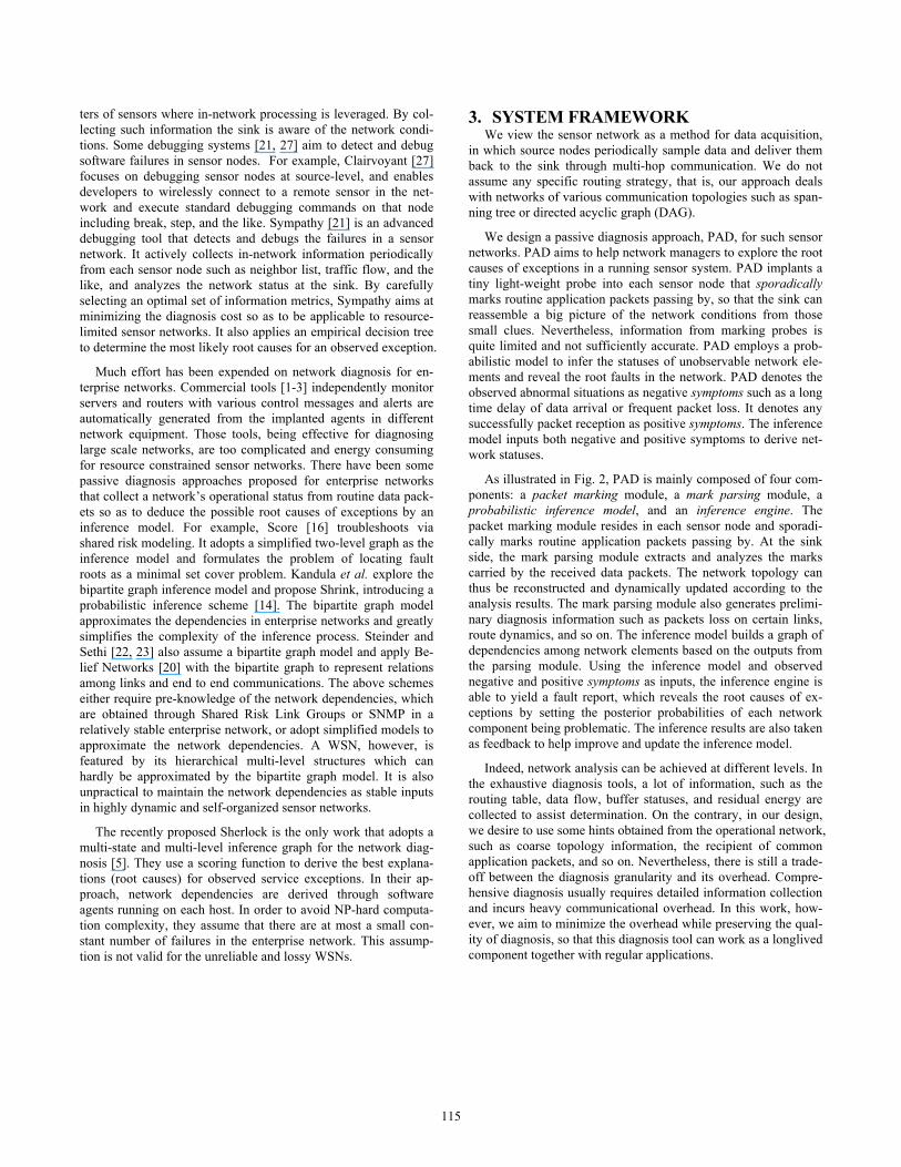
As illustrated in Fig. 2, PAD is mainly composed of four com-ponents: a packet marking module, a mark parsing module, a probabilistic inference model, and an inference engine. The packet marking module resides in each sensor node and sporadi-cally marks routine application packets passing by. At the sink side, the mark parsing module extracts and analyzes the marks carried by the received data packets. The network topology can thus be reconstructed and dynamically updated according to the analysis results. The mark parsing module also generates prelimi-nary diagnosis information such as packets loss on certain links, route dynamics, and so on. The inference model builds a graph of dependencies among network elements based on the outputs from the parsing module. Using the inference model and observed negative and positive symptoms as inputs, the inference engine is able to yield a fault report, which reveals the root causes of ex-ceptions by setting the posterior probabilities of each network component being problematic. The inference results are also taken as feedback to help improve and update the inference model.

Indeed, network analysis can be achieved at different levels. In the exhaustive diagnosis tools, a lot of information, such as the routing table, data flow, buffer statuses, and residual energy are collected to assist determination. On the contrary, in our design, we desire to use some hints obtained from the operational network, such as coarse topology information, the recipient of common application packets, and so on. Nevertheless, there is still a trade-off between the diagnosis granularity and its overhead. Compre-hensive diagnosis usually requires detailed information collection and incurs heavy communicational overhead. In this work, how-ever, we aim to minimize the overhead while preserving the qual-ity of diagnosis, so that this diagnosis tool can work as a longlived component together with regular applications.

115

Figure 2. PAD system overview

4. PACKET MARKING Since a sensor network has a self-organized time-varying net-

work structure, unlike the case in an enterprise network, no prior knowledge can be obtained for constructing the inference model. Also, as a WSN topology is highly dynamic, we need to acquire the network statuses continually to maintain the topology in real-time. To address the above requirements, we design a packet marking algorithm in PAD, which dynamically captures the net-work topology and extracts the inner dependencies among net-work components. Before the analysis results are directed to the inference engine for further reasoning, we can generate a prelimi-nary diagnosis report on some basic network exceptions.

The main operation of this marking algorithm is to let sensor nodes stamp their IDs on passing data packets. Due to the size limitations of the data packets used in sensor networks, however, the marking scheme only adds two bytes to each data packet that records one node ID. During the packet delivery, only one se-lected sensor node marks its ID and updates the hop count field on each packet based on a set of rules. At the sink side, the mark parsing module traces back the paths from each source node through analyzing sporadically marked packets. Through assem-bling the paths from different source nodes, the network topology can be reconstructed along with the regular data delivery of the system. If the network remains static, the packet marking process automatically converges and stops after the entire network topol-ogy is constructed. When network conditions vary, such as when packet loss or route changes occur, the packet marking process restarts somewhere close to the exceptional event. A strength of this design is that it does not inject any extra message into the network and strictly limits the overhead of marks attached to each data packet.

4.1 Marking Scheme on Sensor Nodes Figure 3 depicts an example of data packet marking. We as-

sume that each original data packet contains (1) a source node ID denoting the source node of this packet, (2) a sequence number identifying the packet, and (3) a hop count recording the number of hops it travels. If there is no such information recorded in the application, the marking scheme adds them to the packets. The

mark added to the original packet is the pass node ID which re-cords the ID of a sensor that participates in delivering this packet. When the source node issues a new data packet, it leaves the pass node ID field empty.

Algorithm 1 Packet_Marking (packet p)

1: if p has been marked 2: return; 3: else 4: check cache; 5: if no entry for source node of p 6: mark p; 7: create entry with source node ID and sequence number in p; 8: else if entry exists and sequence number continuous 9: update entry with new sequence number; 10: increase hop count in p by 1; 11: else if entry exists and sequence number not continuous 12: mark p; 13: update entry with new sequence number; 14: end if 15: end if 16: return;

Every intermediate node maintains a cache for its down-stream source nodes. As illustrated in Fig. 3, each cache entry consists of a source node ID and the sequence number of the recently re-ceived packet from the source. As shown in algorithm 1, upon receiving a packet, an intermediate node first checks whether the packet has been marked. If yes (the pass node ID is not empty), it forwards the packet with no further operations. Otherwise, the node checks its own cache. If there is no entry for the source node ID of this packet, it marks the packet by filling the pass node ID field with its own ID. It also creates a new entry for this source node in its cache and records the sequence number for the packet. If there exists an entry in the cache for the source node and the

116

sequence number in the packet is consistent with the cache entry, the intermediate node updates the cache entry with the new se-quence number. To prevent duplicate marking, the intermediate node does not fill the pass node ID field, instead it increments the hop count in the packet by 1 and forwards the packet. If the se-quence number of the packet is not consistent with that recorded in the cache entry, it might be due to the packet loss or routing variations. The intermediate node marks the packet by filling the packet pass node ID field with its own ID. The node then updates its cache entry with the new sequence number of this packet and forwards it. The sink also participates in the marking process and creates a table recording source nodes and their packet sequence numbers. Using this marking scheme, the received packet in the sink records the ID of one intermediate node in the routing path together with its hop count to the source node. We avoid duplicate marks of the same node on the same path to save communication costs. We can further reduce the memory usage in each sensor node by organizing its cache table into bloom filters. Each inter-mediate node inserts and extracts the source node information on the bloom filter. The error rate introduced by the bloom filter introduces negligible adverse impact in the lossy by-nature sensor network.

4.2 Parsing the Marks At the sink, the mark parsing module extracts and parses the

marks piggybacked from the received packets. For each source node, we keep a data structure denoted as path to record node IDs along the path from the source node to the sink. A path contains an array of slots and each slot records a node ID along the path hop by hop. The path also has a field which records the sequence number of the latest arrived packet from each source.

On receiving a new packet, the mark parsing module checks the existence of a path structure associated with its source node. If there is no such path, it means it is the first time the sink has re-ceived packets from that source. The sink creates a new path for the source node and records the source node ID at the first slot. The mark parsing module then examines whether the packet has been marked (the pass node ID field has been filled). If it has been marked, the sink updates the associated slot in the path to be the recorded node ID according to the hop count in the packet.

For the packets from the recorded path, the parsing module op-erates according to the recorded sequence number. We denote d as the difference between the sequence number of the received packet and the sequence number recorded in the path. Normally,

without packet loss, d = 1, and we directly add the marked node ID into the path. Inconsistence of the sequence numbers (d > 1) indicates that the packet loss occurs and triggers a preliminary diagnosis report on packet loss. A mismatch of the recorded pass node ID in the packet and the recorded node ID in corresponding slot in the path indicates a route variation at the hop count re-corded in the packet and its d hops upwards, otherwise the mark-ing should be taken earlier. The parsing algorithm then generates a preliminary report of a route switch. In such a case, the recorded path from d hops before the hop count position to sink becomes inaccurate, so we clear all those slots. The reception of the packet without any marks triggers a preliminary report of a successful delivery. The mark parsing function is shown in algorithm 2.

The mark parsing module constructs and updates the network topology with the recorded paths. Once a new packet is received, the path associated to its source node is updated. This indicates that all links along the current path have just participated in the transmission of a packet. For each link in the network topology, we keep a counter to count the number of transmissions experi-enced by this link. Such information facilitates the construction of the inference model as it tells the strength of the dependency be-tween the parent and its successive nodes.

Obviously, the number of packets we need for capturing the entire path for a source node is at most the maximum hop count. Even under frequent route switches, the number can be bounded to a small constant. Since links in sensor networks are usually shared by many paths, we do not need to collect path information for all paths before we are able to construct the complete network topology. Indeed, our packet marking scheme captures the net-work topology with a small number of packet receptions, as dem-onstrated in our field experiment.

Algorithm 2 Mark Parsing(packet p)

1: if p.sourceNodeID has no associated path 2: create new path for p.sourceNodeID; 3: end if 4: d = p.sequenceNumber – path.sequenceNumber; 5: if d <= 1 //no packet loss 6: if path[hopCount] != p.passNodeID //route switch 7: path[hopCount] = p.passNodeID; 8: clear all slots in path after path[hopCount]; 9: generates route switch report; 10: end if 11: else //packet loss detected 12: generate packet loss report; 13: if path[hopCount] != p.passNodeID //route switch 14: clear all slots in path after path[hopCount - d]; 15: path[hopCount] = p.passNodeID; 16: end if 17: end if

Clearly, in this design we propose to mark simple messages

only; but if we insert more marks into the data packets, we obtain richer information on the network statuses and make the diagnosis process more straightforward. Nevertheless, in resource con-strained sensor networks, we have to minimize the communica-

Figure 3. The marked data packet and the cache content of intermediate nodes

117

tion overhead introduced by our diagnosis model. Therefore, we choose to only use simplified marks to additively reconstruct the network. We give details about this issue in later discussions.

4.3 Preliminary Diagnosis Reports Before the final diagnosis results are obtained from the infer-

ence engine, some preliminary diagnosis reports can be yielded from the mark parsing module, which help to analyze the network statuses. The preliminary diagnosis briefly infers the following reports.

1) Success delivery report. When the sink receives a packet with-out any mark, it indicates a successful delivery along the cur-rent path. This report tells us that the route from the source sensor node to the sink is still the same and all links along this path have just conducted a successful transmission that con-firms the active state of those links.

2) Packet loss report. As described above, if the difference d be-tween the sequence number recorded in the path and the se-quence number of the packet is more than one, it can be in-ferred that the packet loss occurs. The number of packet loss is quantified as d - 1. In this case, according to our marking scheme, the packet must have been marked by some interme-diate node. This report can further locate the packet loss loca-tion if there is no route switch accompanying the packet loss.

3) Route Switch Report. The mismatch of the pass node ID in the packet and the recorded ID in the corresponding slot in the path indicates that the previous routing path has been altered. The position of the switch is between the hop count recorded in the packet and d hops upward.

5. PROBABILISTIC INFERENCE The packet mark parsing module provides a coarse abstraction

and incomplete report. At the sink, the successive probabilistic in-ference helps to reveal the inner dependencies among different net-work elements in the sensor network and expose the hidden root causes of the exterior symptoms. Network elements are inner corre-lated, for example, the crash of an upstream node causes all its chil-dren to disconnect from the sink. In contrast, simultaneous conges-tion of multiple paths may indicate a high probability of a malfunc-tion at a common link. Based on such observations, we explore the dependencies among network elements (link status, sensing function, path status, etc.) on the constructed communication topology and encode them with a probabilistic model. Exterior symptoms like delay or loss of data samples are considered as inputs. When spe-cific symptoms are observed by our inference algorithm, we can deduce the probability of the failures of each network element and find the most probable root causes.

We first apply the Belief Network [20] as our inference model. Belief Network is a well-known probabilistic model that has been widely used in research domains like artificial intelligence and system engineering. In Belief Network, each possible root cause or symptom is represented by a variable. Each variable might have multiple values (e.g. 1 for a link in active state and 0 for in trou-ble). Causal relationships between different variables are denoted as directional arcs. Inferences can be conducted on this model to deduce the probability of particular values to our interested vari-ables once the values of some other variables have been observed (e.g. symptoms like the high delay of data samplings). To further

speedup the process, we propose a simplified inference model, Causality Diagram. According to the characteristics of sensor networks, we can design a simplified Causality Diagram which accurately approximates the inference results and reduces the overhead.

5.1 Belief Network A Belief Network (or Bayesian Network) is a Directed Acyclic

Graph (DAG) that represents a set of variables and their probabil-istic relationships. Each vertex in the graph denotes a random variable. In the rest of this paper, we use “vertex” and “variable” interchangeably. A directional arc connecting vertex X1 to X2 indicates a causal relation between the two variables. The cause X1 is called a parent of the outcome X2. The strength of the rela-tion between a parent and its child is defined by the conditional probabilities. We then formulate a Belief Network as a binary (G, P), where G = {V, E} is a DAG and P = {Pi} specifies a Condi-tional Probability Distribution (CPD) in G. Here, V = {Vi} repre-sents the set of vertices in G, and E = {Ej} denotes all arcs (or edges). Pi specifies the conditional probability distribution of each variable given its parents. When the value domain of variable is discrete, the CPD can be represented as a Conditional Probability Table (CPT).

Figure 4 illustrates a simple example of a Belief Network which contains four variables A, B, C and D. Each variable has two possible discrete values denoted as True and False. The ta-bles associated with variables in Fig. 4 specify their CPTs. For example, variable D has two parents B and C, so each entry in its CPT gives the probability of D to take a certain value given the particular assignment of B and C. Since variable A has no parents, its CPD is a prior probability distribution.

Given certain evidence (values of some variables), the Belief Network can answer three major types of queries[20]: 1) Posterior probability assessment, 2) Maximum posterior hypothesis, and 3) Most probable explanation. The first type of query, which esti-mates posterior probabilities of certain variables given some evi-dence variables, best fits our requirements in this work. For ex-ample, in the Belief Network in Fig. 4, while given D = True, the posterior probability of B = True and C = True can be calculated as follows.

Figure 4. The Belief Network

118

)Pr(

),,,Pr()Pr(

),Pr()|Pr(

,

TrueD

TrueDcCTrueBaATrueD

TrueDTrueBTrueDTrueB

ca

=

=====

===

===

∑,

)Pr(

),,,Pr()Pr(

),Pr()|Pr(

,

TrueD

TrueDTrueCbBaATrueD

TrueDTrueCTrueDTrueC

ba

=

=====

===

===

∑,

Where

∑ ======cba

TrueDcCbBaATrueD,,

),,,Pr()Pr( .

5.2 Inferring through Belief Network Our inference model automatically constructs and maintains a

Belief Network from the output of the mark parsing module. The inference engine accordingly infers from this model hidden statuses of the network. In our PAD approach, the Belief Network structure is assembled from the current network topology obtained from the mark parsing module.

5.2.1 Constructing a Belief Network Figure 5 (a) depicts a simple example topology composed of a

sink and three sensor nodes. The directional edge between two nodes denotes a wireless link and the direction of data transmit-ting along the link. There are five types of variables in our Belief Network, each of which has the value domain of {Up, Down} that denotes a normal or abnormal working status, respectively.

For each source node, we add a variable Di to the Belief Net-work which denotes the status of the data reception of the source node. For example, if the sink observes a long time delay in the data reception from a source, the corresponding Di variable of this node will be set to Down. Note that in many applications some sensor nodes do not sample data but only relay messages for other nodes. Some of the nodes simply relay packets for other sensors, so there are no data reception variables for those nodes. The status of the data report variable Di depends on two parent variables, the sensing variable Si and the connection variable Ci. The sensing variable Si indicates the sensing function of the corresponding source node and the connection variable Ci describes the condi-tion of the network connectivity from the source node to the sink. We add two arcs from Si and Ci to Di to represent the dependen-cies between them. Si and Ci are thus called the parent variables of Di in the Belief Network. Both the sensing functionality and the network connectivity condition will affect the success of the data reported from the source node.

The connectivity from a source node to the sink relies on one or more paths connecting them. For example, node 2 in Fig. 5(a) can choose to deliver packets through two parents; node 1 and node 3, so in the corresponding Belief Network the connection variable C2 has two parent variables P2-1-0 and P2-3-0. They are called path variables. The subscript of each path variable sequen-tially denotes the ID of the start node on the path, the ID of the next hop node from the start node, and the ID of the end node on the path. As illustrated in Fig. 5(b), the status of each path vari-able depends on two parent variables. One is the link variable on

the first hop from the start node and the other is the connection variable of its parent node. The link variable Lm-n represents the communication conditions of a wireless link between two nodes m and n.

We connect each pair of variables that has a dependency with a directional arc from the cause variable to the outcome variable. Eventually we obtain a hierarchical network composed of these five types of variables in which dependencies among network elements are encoded. Among the five types of variables, the statuses of the link and sensing variables are hidden from the exterior observations that most need to be inferred. The path and connection variables are intermediate variables which are usually combinational results of other parent variables. The data report variables are outputs of the mark parsing module that we directly observe at the sink. The Belief Network structure consisting of the variables is automatically maintained and updated when network topology and communication conditions vary over time.

5.2.2 Inference on Belief Network Once the Belief Network structure is constructed, a critical is-

sue is how to assign CPTs for variables that specify the condi-tional probabilities between parents and their children. Different logistic relations between parents and their children lead to differ-ent methods for calculating the CPT. For example, the sensing variable and connection variable affect their children variable of data report in a logical OR manner, i.e., if one of them is in the Down state, the data report variable should be switched onto the Down state. Due to the diverse routing schemes and high dynam-ics in sensor networks, a sensor may maintain multiple parents for relaying its data. Consequently, in our inference model, multiple path variables affect the same connection variable in SELECT mode where the status of selected paths will determine the status of the connection variable. In PAD, we employ the noisy-OR gate [20] and Select gate [5] to encode these operations.

Figure 6 (a) shows the CPT in a noisy-OR gate where any one of the parent variables in Down status results in the Down status of the child variable. In Fig. 6, h1 and h2 represent the noisy prop-

Figure 5. Belief Network constructed from the communication topology

119

erty that means even if both parent variables are in the Up status, the child variable still has a chance to fail (in Down status). In PAD, noisy-OR gates exist in several cases such as when the sens-ing and connection variables affect the data report variables, the link and connection variables affect the path variables, and so on. The relation between multiple path variables and a connection variable is represented by the Select gate as illustrated in Fig. 6 (b). Here d denotes the dependency strength of each parent and in the case of Fig. 6 (b), d is the probability that the child connection variable selects a certain path to relay data. Thus, the probability that a connection variable is in the Up status is given by

∑ ===

UpP inii

dPPPPUpchild )...,...,|Pr( 21 .

In the Belief Network, each noisy-OR gate connects two parent variables to a child variable, so the CPT calculation is quick. The Select gate might connect more parent variables to a child vari-able but the maximum number of parent variables for one gate is bounded by the number of neighbors for a sensor node. The num-ber of neighbors is normally treated as a constant. Hence, the CPT calculation for Select gate is also efficient. In the initial stages, the prior fault probability distribution of the link and sensing vari-ables are assigned according to experience data. The value of each di is assigned by estimating the percentage of transmissions deliv-ered through each path in a connection. Such information is input from the mark parsing module.

The outputs of the inference process are the status estimations about the link and sensing variables. Such estimations reveal deeper understanding of the network operation. For example, a single link failure might be caused by environmental interference to the wireless communications, and multiple weak links relating to one sensor node might indicate a faulty node. We have more discussions in Section 6 on how we detect the network faults from the output of our inference process.

5.3 Fast Inference Scheme The Belief Network model is a widely used tool in dealing

with inference tasks that achieve high performance even with incomplete or suspicious inputs. The inference process in a gen-eral Belief Network, however, is NP-Hard [8], and even some approximate approaches have been proven to be NP-Hard [9].

While previous studies in comparatively stable enterprise net-works are able to simplify [22, 23] the Belief Network into bipar-tite graphs or polytrees, the hierarchical multi-level characteristic of sensor networks makes it impractical. To speedup the inference for large scale sensor networks, we further propose a new infer-ence model based on the Causality Diagram [30].

Similar to Belief Network, Causality Diagram is a graphic in-ference model. Instead of conditional probability, Causality Dia-gram uses dependency strength to represent the relationships be-tween vertices and exploit logistic computation in the probabilis-tic inference process.

As shown in Fig. 7, a Causality Diagram is a directed graph consisting of four types of elements including basic events, inter-mediate events, arc events and logic gates. Each vertex or arc in a Causality Diagram denotes an event. Rectangles like B1 denote the basic events that are independent causes of other events. Cy-clic vertices like X5 represent intermediate events that can be out-comes or causes of other events. An arc connecting two vertices is called an arc event that specifies a causal relation between the two events. The associated strength on an arc denotes the probability that the parent event affects its child event. Note that if there is no additional parameter on an arc, it means that the parent event has an impact on the child event at a probability of 1. The logic gates like G5 specify how multiple parent events jointly influence one child event.

Taking the same example network topology in Fig. 5, Fig. 8 shows how to construct a Causality Diagram for our inference engine. Different from that in Belief Network, each vertex in a Causality Diagram denotes a fault event. Those vertices without parents (rectangular in shape) are basic events that are independ-ent root causes. Other cyclic vertices denote intermediate events.

The traditional inference algorithm is NP-hard [30] on general Causality Diagrams and is thus infeasible for our approach. Nev-ertheless, in this design, due to the characteristics of WSNs, we are able to use only OR and Select gates to model the dependency relationships between node behaviors. This enables us to apply a fast inference scheme, leveraging the particular structure of our model. Our scheme contains four stages:

1) We represent each intermediate event by its first order cut set (CS1) expression.

2) We adopt an early disjointing mechanism. Before generating the final cut sets (CSf) expressions, we directly disjoint the CS1 expressions. Based on the definition of the Select gate, the cut sets in a CS1 expression of the connection failure events are already exclusive.

3) We calculate final disjoint cut sets (DCSf) expressions by it-eratively replacing intermediate events in each expression. Since all negative events generated from step 2 are basic events, we avoid the complex NOT operations and the replacement process can be oper-ated efficiently.

4) We estimate the posterior probabilities of user specified events. Given observed events E (evidences), we can calculate the posterior probability of interested events H (root causes). E = E1 ∩ E2 ∩…∩ Ek. According to the Bayesian formula:

Figure 6. CPTs of noisy-OR and select gates

120

)Pr()Pr(

)Pr()Pr(

)(Pr)Pr()|Pr(

21

21

k

k

EEEEEEH

EEH

EHEEH

III

IIIII

⋅⋅⋅⋅⋅⋅

===

Both H and Ei have been expressed as DCSf and the result of operating logic AND on two DCSf expressions is still a DCSf expression. Hence, expressions on numerator and denominator are both DCSf and the posterior probability of H can be calculated algebraically.

6. CHARACTERIZING THE FAULTS After the inference process, both the packet mark parsing module

and the inference engine output the fault reports about the sensor network statuses. In this section, we discuss how PAD further char-acterizes the faults in the network through timely analysis of the fault reports.

Compared with enterprise networks, WSNs are highly dynamic and suffer more from environmental variations. As such, the possi-ble faults in WSNs are much more complex than in enterprise net-works where the network faults can simply be characterized as host or link failures. For example, most of the time, the failure of com-munication among a group of sensor nodes is not due to hardware or software failures, but because of a temporal interference from an outside environment. According to the complexity of sensor net-work faults, in PAD, we trace the fault reasons by characterizing their fault patterns as follows.

1) Physical damage. In many field applications, physical damage might occur and destroy a portion of or the entire hardware of sen-sor nodes. For example, the battery component usually falls off the mote board due to the ocean waves, as we already experienced in our sea monitoring project. The sensing unit of a sensor node can also be damaged by cruel environment conditions. To locate the physical damage to a sensor node, we need to confirm its faults for a long period without obtaining any positive symptoms, for example, when there is no successful transmission report from all observed links associated with that sensor node, our inference engine outputs a high error probability of both sensing and communication func-tions for the node. The route switch of the child nodes that previ-ously used this node to relay data will enhance the belief in the physical failure of the node. When a physical fault is detected, the repair actions include checking sensor nodes or redeploying sensors in the certain region.

2) Software crashes. Software crashes include local problems on the sensor node such as a send queue overflow or busy CPU in those nodes that are physically intact. PAD detects the sensor nodes in a software crash by both the diagnosis information from the mark parsing module and the posterior probability estimations from the inference engine. If all the links around a certain node are reported to lose an extraordinary amount of packets with sporadic successful transmissions, PAD issues a software crash report at this node. PAD distinguishes a software crash from physical damage by the sporadic positive feedback like successful packet delivery or establishment of new links around the node. To repair the software crash faults, the sink can issue reboot commands to targeted sensors.

3) Network congestion. Network congestion relates to a group of sensors or traffic flows. The occurrence of network congestion usu-ally leads to a high packet loss rate within the influenced region. However, unlike the case of physical damage, there are still some positive reports from the targeted source nodes. Due to such a fea-ture of this type of faults, the observed symptoms are usually tempo-ral and distributed across a large time and space span. In our imple-mentation experiment, we examine the burst loss rate for each link and the sequence of normal and lossy links to identify congestion. One way of repairing network congestion faults is to decrease the data generation at source nodes.

4) Environmental interferences. Environmental interference can significantly degrade the performance of WSNs even without any internal problems within the WSN itself. The environment interfer-ence usually has high spatial correlation, that is, a large number of nodes in the same region experience degradation of performance at the same time. We infer environment interference as the root cause by observing link degradation across a wide area and lasting for a certain time period. To address this issue, a network manager needs to check the possible sources of interference and reduce the work-load or even temporarily turn off some nodes to protect them from unnecessary physical damage or power wastage.

Figure 7. The Causality Diagram

Sink

D2

S2

C2

L21

C1L10

L23

C3

Pa210 Pa230D1

S1

Pa310

L31

S3

D3

OR gate

Select gate

L SLink failure event Sensing failure event

P Path failure event C Connection failure event

D Data report failure event

(a)(b)

P210 P230

0

2 3

1

Figure 8. The Causality Diagram constructed from the commu-nication graph

121

5) Application flaws. As the application programs might con-tain flawed components, the network might suffer from some inefficiency that does not lead to system crashes but consumes computational or communicational resources. A typical example is the instability of the routing selection. Indeed, when we apply PAD to our sea monitoring project, we observe frequent route switches for the packet delivery, incurring a large amount of con-

trol messages to the network but no improvement to the commu-nication quality. This observation confirms our suspicions about the rapid depletion of sensor energy. Such types of faults are usu-ally highly related to the applications and are indeed difficult for a light-weight network diagnosis tool to detect without any applica-tion control information. It is more like a byproduct of PAD.

7. EVALUATION We conduct comprehensive simulations and implement field

experiments to evaluate the performance of PAD. For the imple-mentation, we used the BNJ implementation of the Belief Net-work inference as part of our inference engine. We implemented the packet marking scheme for TelosB motes on the TinyOS plat-form with nesC language. We implemented the mark parsing module on the java based back end.

7.1 Simulations We first examine the effectiveness and efficiency of PAD

through simulations. We simulate a sensor network on the java platform which is organized into grids, with the sink located at the centre. Sensors periodically generate data and deliver to the sink through multi-hop routes. Two routing schemes are applied in the simulation. Various types of faults are inserted into links or nodes according to different test settings.

20 30 40 50 600.7

0.75

0.8

0.85

0.9

0.95

1

Network Size

Det

ectio

n R

ate

BN-TreeCD-TreeBN-DAGCD-DAG

20 30 40 50 600.1

0.15

0.2

0.25

0.3

0.35

0.4

Network Size

Fals

e P

ositi

ve R

atio

BN-TreeCD-TreeBN-DAGCD-DAG

Figure 10 (a) Sensing failure detection rate Figure 10 (b) Sensing failure false positive ratio

0 20 40 60 80 1000

100

200

300

400

500

Network Size

Num

ber o

f Pac

kets

TreeDAG

Figure 9. Convergence time on varying network sizes

122

20 30 40 50 600.5

0.6

0.7

0.8

0.9

1

Network Size

Det

ectio

n R

ate

BN-TreeCD-TreeBN-DAGCD-DAG

20 30 40 50 600

0.1

0.2

0.3

0.4

0.5

Network Size

Fals

e P

ositi

ve R

atio

BN-TreeCD-TreeBN-DAGCD-DAG

Figure 11 (a) Node failure detection rate Figure 11 (b) Node failure false positive ratio

1 2 3 4 50.75

0.8

0.85

0.9

0.95

1

Number of Faults

Det

ectio

n R

ate

BNCD

1 2 3 4 50

0.05

0.1

0.15

0.2

0.25

Number of Faults

Fals

e P

ositi

ve R

atio

BNCD

Figure 12 (a) Detection rate for multiple faults Figure 12 (b) False positive ratio for multiple faults

7.1.1 The efficiency of the packet marking scheme We evaluate the convergence time of the packet marking scheme

under various network conditions. In this test we simulate a data acquisition network using both spanning tree based routing and DAG based routing schemes. We measure the convergence time by counting the number of data packets needed for constructing the entire network topology. The smaller number of packets needed indicates faster convergence. Different routing schemes lead to different types of topologies. Term Tree denotes a spanning tree topology rooted at the sink and DAG represents a multi-path routing strategy where each sensor node has multiple parents. Figure 9 shows the number of packets required in the packet marking process under the two topologies. For both cases, the number linearly in-creases as the network size increases. In other words, the average packets sent from each source node is relatively stable. The DAG network has a more complicated topology, so the marking scheme requires more packets to figure it out.

7.1.2 The performance of inference models We then evaluate the performance of the two inference models

with four different groups of tests. We inject artificially created errors into the network and let both inference models generate fault reports according to the posterior probability estimations.

We first inject sensing failures into sensor nodes and compare the detection rate and false positive ratio of both models. We randomly invalidate the sensing capabilities of 10% of the nodes. BN-Tree and BN-DAG denote inference results of the Belief Network model on the spanning tree topology and DAG topology. CD-Tree and CD-DAG represent the inference results of Causality Diagram model. We vary the network size from 16 nodes to 64 nodes. Figure 10 (a) plots the detection rates, where we can see both models achieve detection rates higher than 90% in most situations. Belief Network model has a slightly higher detection rate than Causality Diagram model as it adopts exactly accurate inference. Figure 10 (b) shows the false positive ratio of the two models. We see that for both two models, the false positive ratio decreases as the network size increases. By analyzing the false reports, we find that most

123

false positive reports relate to the leaf nodes. As those nodes lie on the boundary of the network field and do not relay data for others, if they do not report data to sink, there are few clues as to whether it is due to a sensing failure or a communication failure.

We then inject node failure of both sensing and communication errors into sensor nodes; see Fig. 11 for the results. As the network size increases, the detection rate decreases and the false positive ratio increases. Both inference models achieve comparable detection rates under different topologies while Belief Network is slightly better than Causality Diagram with a lower false positive ratio.

We conduct simulations to test how the inference models per-form against multiple errors in the network. In this test, we simulate a network with 25 sensor nodes. We randomly select 1 to 5 sensor nodes and simultaneously insert errors into them. The results are shown in Fig. 12. We find that when multiple faults simultaneously occur, the detection rate decreases and the false positive ratio in-creases. This is because the existence of multiple errors introduces mutual interference in the inference model and degrades the per-formance. As Fig. 12 shows, a single error is easy to detect and 5 simultaneous errors lead to worse results.

The last group of simulations compares the computational effi-ciency of the two inference models. As shown in Fig. 13, the com-putation overhead of Belief Network is much larger than Causality Diagram and their difference increases quickly as the network size increases. Although as previous simulation shows, Causality Dia-gram model provides approximated inference with less accuracy than the Belief Network model, it largely reduces the computational overhead and thus is more viable for practical usage.

7.2 Implementations and Field Experiments We implement and test the effectiveness of the PAD approach

through a field study in our sea monitoring sensor network system [28]. The experiment is conducted over a long period and we fetch and analyze a segment of 22,416 received packets as well as the marks in them.

7.2.1 Observations in the field study The analysis results from PAD confirm our concern about the

energy efficiency of the system. We indeed observe extraordinarily high frequency of topology variations in the sensor network. Figure 14 compares the topology variations with the packet receptions during the sea monitoring system operation. We summarize the number of topology variations throughout each ten minutes interval. From results in Fig. 14 (a), we find that every ten minutes there are topology variations of 10 to more than 40 times that in the network. As shown in Fig. 14 (b), however, there is no apparent correspon-dence between the topology variations and the packet receptions. Thus, most of the topology variations occur but do not significantly improve the network communication quality. Figure 15 exhibits a group of topology snapshots of a certain region in the network. The interval between each pair of consecutive subfigures is two minutes. According to the algorithm used in the MultiHopRouter component, the topology variations indeed always incur large traffic overhead in the network.

This observation confirms our concern that the network quickly depletes the node energy due to the frequent route switches, while most of them occur because of the instability of link quality between the floating sensor nodes. Clearly, frequent route switches may lead to high energy cost that largely con-strains the lifetime of our monitoring system. We improve our application program by setting adequate redundancy in measuring

40 60 80 1000

500

1000

1500

2000

Network Size

Tim

e (m

illis

econ

d)

BNCD

Figure 13. Computation time of two inference models

0 20 40 60 800

10

20

30

40

Time (10 minutes)

Num

ber o

f Top

olog

y C

hang

es

Topology Variation

Figure 14 (a) Topology variation statistics over time

0 20 40 60 800

100

200

300

400

Time (10 minutes)

Num

ber o

f Rec

eive

d P

acke

ts

Packet Reception

Figure 14 (b) Packets reception statistics over time

124

the link quality and switching the routes. Currently, our system has been operating neatly with much fewer unnecessary routing dynamics.

7.2.2 Traffic overhead Through analyzing the received packets, we compare the extra

overhead introduced by PAD and Sympathy. We use empirical cumulative distribution functions (ECDF) to quantify the over-head. In Fig. 16, the x axis denotes the ratio of the diagnosis over-head to the total network traffic and the y axis denotes the ECDF. For example, a point with value (0.3, 0.8) on x and y axes respec-tively indicates the fact that 80% of the time, the diagnosing transmission dominates less than 30% of the total network traffic. A curve to the left represents a small cumulative overhead. Dif-ferent curves for the Sympathy approach denote the cases of dif-ferent report intervals in sending the diagnosis metrics. As Fig. 16 shows, PAD significantly outperforms Sympathy in terms of the traffic overhead.

7.2.3 Diagnosis for the problematic network In this experiment, we artificially inject sensing and communi-

cation faults into two sensor nodes respectively and mix them into the network. We let the two nodes interchangeably work under normal and exceptional statuses. We turn off the wireless radio of one sensor node (NodeA) every 5 minutes and invalidate the sens-ing module of the other node (NodeB) every 5 minutes. As shown in Fig. 17, the red curve represents the inferred posterior fault probability of the sensing functionality in NodeB. The inference result accurately captures the periodical faults of the sensing module in NodeB. The three other curves denote the inferred fault probabilities of three links associated with NodeA which indicate the faults in those links. We can see that PAD correctly captures the periodical communication failures of NodeA. According to Sympathy performance report, Sympathy is able to detect any failure injected into the network if the system parameters are properly set. From our experimental results, as a comparison,

PAD achieves more than a 90% detection rate and around 80% accuracy, but with significantly reduced overhead.

8. CONCLUSIONS AND FUTURE WORK Although there have been many approaches proposed for de-

bugging the operation of sensor network systems in a controlled laboratory, few works have been done towards an in-situ diagno-sis tool for monitoring the statuses of operational systems in the field. In this paper, we propose PAD, a passive diagnosis approach, which can be efficiently implemented and applied to a normally working sensor network system providing in-situ network diagnosis. The proposed light-weight packet marking scheme collects neces-sary hints without injecting extra traffic overhead to the original system. The probabilistic inference model residing at the sink cap-tures the unique features of the sensor networks and yields accurate results. The inference engine works well even with incomplete or suspicious inputs in a nondeterministic manner. We implement our diagnosis approach and validate its effectiveness in a field test in our sea monitoring project. The sea monitoring project is an undergoing project. We are currently utilizing PAD as an important diagnosis tool to detect possible faulty components in the system and guaran-

Figure 15. Topology evolutions over time in field study

0 5 10 15 20 25 30 350

0.2

0.4

0.6

0.8

1

Overhead (%)

EC

DF

PAD9 min Sym.6 min Sym.3 min Sym.

Figure 16. System overhead (PAD v.s. Sympathy)

0 5 10 15 200.2

0.4

0.6

0.8

1

Time (minute)

Faul

t Pro

babi

lity

NodeA-Link1NodeA-Link2NodeA-Link3NodeB-Sensing

Figure 17. Diagnosis results for detecting the manually in-jected faults in our field study

125

tee its correct operations. On the other hand, we are relying on such a platform to further test the effectiveness and efficiency of PAD and hope to improve it according to our future observations.

ACKNOWLEDGEMENT The authors would like to thank the shepherd, Deepak Ganesan,

for his constructive feedback and valuable input. Thanks also to anonymous reviewers for reading this paper and giving valuable comments. This work is supported in part by the Hong Kong RGC grant HKUST6169/07E, the National Basic Research Program of China (973 Program) under grant No. 2006CB303000, the National High Technology Research and Development Program of China (863 Program) under grant No. 2007AA01Z180, HKUST Nansha Research Fund NRC06/07.EG01, and NSFC Key Project grant No. 60533110.

REFERENCES [1] "IBM Tivoli," http://www.ibm.com/software/tivoli/ [2] "HP Openview," http://www.openview.hp.com/ [3] "Microsoft Operations Manager,"

http://www.microsoft.com/mom/ [4] "OceanSense: Sensor Network for Sea Monitoring,"

http://www.cse.ust.hk/~liu/Ocean/index.html [5] P. Bahl, R. Chandra, A. Greenberg, S. Kandula, D. Maltz, and

M. Zhang, "Towards Highly Reliable Enterprise Network Ser-vices Via Inference of Multi-level Dependencies," In Proc. of ACM SIGCOMM, 2007.

[6] X. Bai, D. Xuan, Z. Yun, T. Lai, and W. Jia, "Complete Opti-mal Deployment Patterns for Full-Coverage and k-Connectivity (k <=6) Wireless Sensor Networks," In Proc. of ACM MobiHoc, 2008.

[7] J. Cao, L. Zhang, J. Yang, and S. Das, "A Reliable Mobile Agent Communication Protocol," In Proc. of IEEE ICDCS, 2004.

[8] G. Cooper, "Probabilistic Inference using Belief Networks is NP-Hard," Stanford Knowledge Systems Laboratory, Techni-cal Report 1987.

[9] P. Dagum and M. Luby, "Approximately Probabilistic Reason-ing in Bayesian Belief Networks is NP-hard," Artificial Intelli-gence, pp. 141-153, 1993.

[10] Q. Fang, J. Gao, and L. Guibas, "Locating and Bypassing Routing Holes in Sensor Networks," In Proc. of IEEE INFO-COM, 2004.

[11] R. Ganti, P. Jayachandran, H. Luo, and T. Abdelzaher, "Data-link Streaming in Wireless Sensor Networks," In Proc. of ACM SenSys, 2006.

[12] B. Gedik, L. Liu, and P. Yu, "ASAP: An Adaptive Sampling Approach to Data Collection in Sensor Networks," IEEE Transactions on Parallel and Distributed Systems (TPDS), vol. 18, pp. 1766-1783, 2007.

[13] T. He, S. Krishnamurthy, J. Stankovic, T. Abdelzaher, L. Luo, R. Stoleru, T. Yan, L. Gu, J. Hui, and B. Krogh, "Energy-Efficient Surveillance System using Wireless Sensor Net-works," In Proc. of ACM MobiSys, 2004.

[14] S. Kandula, D. Katabi, and J. Vasseur, "Shrink: A Tool for Failure Diagnosis in IP Networks," In Proc. of MineNet Work-shop at ACM SIGCOMM, 2005.

[15] K. Klues, G. Hackmann, O. Chipara, and C. Lu, "A Compo-nent-Based Architecture for Power-Efficient Media Access Control in Wireless Sensor Networks," In Proc. of ACM Sen-Sys, 2007.

[16] R. Kompella, J. Yates, A. Greenberg, and A. Snoeren, "IP Fault Localization Via Risk Modeling," In Proc. of USENIX NSDI, 2005.

[17] S. Lim, C. Yu, and C. Das, "Rcast: A Randomized Communi-cation Scheme for Improving Energy Efficiency in MANETs," In Proc. of IEEE ICDCS, 2005.

[18] H. Liu, P. Wan, C. Yi, X. Jia, S. Makki, and N. Pissinou, "Maximal Lifetime Scheduling in Sensor Surveillance Net-works," In Proc. of IEEE INFOCOM, 2005.

[19] Y. Liu, Q. Zhang, and L. Ni, "Opportunity-based Topology Control in Wireless Sensor Networks," In Proc. of IEEE ICDCS, 2008.

[20] J. Pearl, Probabilistic Reasoning in Intelligent Systems: Net-works of Plausible Inference: Morgan Kaufmann, 1988.

[21] N. Ramanathan, K. Chang, L. Girod, R. Kapur, E. Kohler, and D. Estrin, "Sympathy for the Sensor Network Debugger," In Proc. of ACM SenSys, 2005.

[22] M. Steinder and A. Sethi, "Increasing Robustness of Fault Localization Through Analysis of Lost, Spurious, and Positive Symptoms," In Proc. of IEEE INFOCOM, 2002.

[23] M. Steinder and A. Sethi, "Probabilistic Fault Localization in Communication Systems using Belief Networks," IEEE/ACM Transactions on Networking (TON), vol. 12, pp. 809 - 822, 2004.

[24] M. Varshney, D. Xu, M. Srivastava, and R. Bagrodia, "SenQ: A Scalable Simulation and Emulation Environment for Sensor Networks," In Proc. of IEEE/ACM IPSN, 2007.

[25] J. Wu and S. Yang, "SMART: A Scan-Based Movement-Assisted Sensor Deployment Method in Wireless Sensor Net-works," In Proc. of IEEE INFOCOM, 2005.

[26] N. Xu, S. Rangwala, K. Chintalapudi, D. Ganesan, A. Broad, R. Govindan, and D. Estrin, "A Wireless Sensor Network For Structural Monitoring," In Proc. of ACM SenSys, 2004.

[27] J. Yang, M. Soffa, L. Selavo, and K. Whitehouse, "Clairvoyant: A Comprehensive Source-Level Debugger for Wireless Sensor Networks," In Proc. of ACM SenSys, 2007.

[28] Z. Yang, M. Li, and Y. Liu, "Sea Depth Measurement with Restricted Floating Sensors," In Proc. of IEEE RTSS, 2007.

[29] H. Zhai and Y. Fang, "Impact of Routing Metrics on Path Ca-pacity in Multi-rate and Multi-hop Wireless Ad Hoc Net-works," In Proc. of IEEE ICNP, 2006.

[30] Q. Zhang, "Probabilistic Reasoning Based on Dynamic Causal-ity Trees/Diagrams," Reliability Engineering and System Safety, vol. 46, pp. 202-220, 1994.

[31] J. Zhao, R. Govindan, and D. Estrin, "Residual Energy Scan for Monitoring Sensor Networks," In Proc. of IEEE WCNC, 2002.

126