adaptive risk management in mining project development: a ...

ADAPTIVE RISK MANAGEMENT IN MINING PROJECT DEVELOPMENT:

A FLEXIBLE APPROACH TO IMPROVE RISK RESPONSE

by

Craig Matthew Rice

B.Eng, Mechanical Engineering, University of Victoria, 2004

M.Eng, Civil Engineering, The University of British Columbia, 2009

A THESIS SUBMITTED IN PARTIAL FULFILLMENT OF

THE REQUIREMENTS FOR THE DEGREE OF

Doctor of Philosophy

in

THE FACULTY OF GRADUATE AND POSTDOCTORAL STUDIES

(Mining Engineering)

THE UNIVERSITY OF BRITISH COLUMBIA

(Vancouver)

October 2021

© Craig Matthew Rice, 2021

ii

The following individuals certify that they have read, and recommend to the Faculty of Graduate and Postdoctoral Studies for acceptance, the dissertation entitled:

Adaptive Risk Management in Mining Project Development: A Flexible Approach to Improve Risk Response

submitted by Craig Rice in partial fulfillment of the requirements for

the degree of Doctor of Philosophy

in Mining Engineering Examining Committee:

W. Scott Dunbar, Professor, Department Head, Norman B. Keevil Institute of Mining Engineering, UBC Supervisor

Franco Oboni, PhD, President, Oboni Riskope Associates Inc. Supervisory Committee Member

Omar Swei, Assistant Professor, Department of Civil Engineering, UBC Supervisory Committee Member

Sheryl Staub-French, Professor, Department of Civil Engineering, UBC University Examiner

John Steen, Associate Professor, Norman B. Keevil Institute of Mining Engineering, UBC University Examiner

iii

Abstract

Capital project development is the mechanism through which mining companies turn promising

orebodies into profitable mines. However, broad-scale project success is elusive, with projects

frequently exceeding approved cost and schedule estimates. Researchers and mining

professionals have pointed to project risk management as a way to improve project success.

Despite mature project risk management practices and widespread adoption, projects still

repeatedly fail. This is due partly to the current risk management paradigm of prediction and

advanced planning, with risks frequently materializing differently than predicted. One method of

addressing uncertainty underlying project risks is by embracing flexibility and using an adaptive

management approach to risk response. This dissertation demonstrates how adaptive project risk

management can preserve project value and reduce time to resolve risks.

This dissertation first establishes the state of project risk management practices in mining

through an exploratory survey of industry practitioners. The survey fills a literature gap by

documenting the methods currently used and attitudes towards them. Next, the adaptive project

risk management framework is proposed, describing a structured, iterative process to pursue

multiple competing response alternatives in parallel. The framework also details how

experimentation, observation, and learning support the adaptive process. A continuous

discounted cash flow model and stochastic simulation address uncertain elements of both the risk

and the risk response alternatives. The system model provides insight into the effects of different

risk responses and the value gained through the adaptive approach.

iv

The adaptive framework and system model are explored through two case studies. The first case

involved multiple adaptive iterations and demonstrates how the adaptive process gathers and

models new information using Bayesian inference while pursuing and dynamically tracking

multiple risk response alternatives. The second case study shows how experiments and pilot tests

can be used to learn more about the risk and viability of risk responses. These cases demonstrate

that an adaptive approach can increase project value, reduce the duration of resolving risks, and

potentially limit downside risk compared to a non-adaptive response. The methods proposed in

this dissertation give decision-makers the tools to manage project risks more effectively and

improve risk management outcomes.

v

Lay Summary

Successfully building new mines is vital to mining companies, but mine construction frequently

goes over budget and schedule. Ineffective risk management is suggested as one of the reasons

for this widespread underperformance. Improved risk management techniques that embrace

flexibility, learning, and adapting to changing information may improve mine construction

budget, schedule, and overall performance.

This research includes three parts aimed at improving risk response decision-making in mining

capital projects. The first part includes a survey of project risk management methods used in

industry and the perceptions of these methods. The second part includes the development of a

process and quantitative tools to value an adaptive approach to risk response. The third part

validates the process and tools through two case studies involving unexpected project risks

during mine design and construction. The results show that an adaptive approach can increase

project value while decreasing the time required to resolve risks.

vi

Preface

This dissertation is the original work of the author, Craig Rice. The research idea was generated

through practical work in project development in the mining sector. The research program,

including the methodology, data analysis, and writing this dissertation, was designed and

completed by the author. The research was supervised by Dr. W. Scott Dunbar at the Norman B.

Keevil Institute of Mining Engineering at the University of British Columbia.

The survey on project risk management in the mining industry presented in Chapter 3 was

conducted under UBC Behavioural Research Ethics Board certificate H18-03272. The case study

interviews that provided data for the Meadowbank case study presented in Chapter 7 were

conducted under UBC Behavioural Research Ethics Board certificate H18-03278.

A preliminary and summary presentation of the adaptive project risk management framework

presented in this dissertation, primarily in Chapter 4, was published in the conference

proceedings of the Risk and Resilience Mining Solutions 2016 conference, held in Vancouver,

BC, in November 2016. This paper was co-authored with Dr. Dunbar. I was the lead researcher

and first author and was responsible for structuring, researching, and writing the article. Dr.

Dunbar reviewed the paper, provided insight and guidance, and contributed to manuscript edits.

vii

Table of Contents

Abstract ......................................................................................................................................... iii

Lay Summary .................................................................................................................................v

Preface ........................................................................................................................................... vi

Table of Contents ........................................................................................................................ vii

List of Tables .............................................................................................................................. xiv

List of Figures ............................................................................................................................. xvi

List of Abbreviations ................................................................................................................. xix

Acknowledgements .................................................................................................................... xxi

Dedication ................................................................................................................................. xxiii

Chapter 1: Framing the Research Opportunity .........................................................................1

1.1 Introduction ..................................................................................................................... 1

1.2 Research Motivation ....................................................................................................... 6

1.3 Research Questions ......................................................................................................... 7

1.4 Methodology ................................................................................................................... 9

1.5 Contribution and Significance ...................................................................................... 11

1.6 Dissertation Structure.................................................................................................... 12

Chapter 2: Literature Review .....................................................................................................14

2.1 Introduction to the Literature Review ........................................................................... 14

2.2 Capital Projects in the Mining Industry ........................................................................ 16

2.3 The Risk Concept .......................................................................................................... 18

2.4 Project Risk Management ............................................................................................. 23

viii

2.5 Managing Uncertainty and Flexibility in Projects ........................................................ 27

2.6 Synthesis of the Literature ............................................................................................ 30

Chapter 3: Survey on Project Risk Management in the Mining Industry .............................32

3.1 Survey Objectives ......................................................................................................... 32

3.2 Survey Design and Methodology.................................................................................. 33

3.3 Multiple Choice Results and Analysis .......................................................................... 34

3.3.1 Respondent Profiles: Survey Section 1 ..................................................................... 35

3.3.2 Exposure to Project Risk Management: Survey Section 2 ....................................... 37

3.3.3 Definitions of Risk: Survey Section 3 ...................................................................... 39

3.3.4 Use and Perception of Risk Management Tools: Survey Section 4 ......................... 42

3.3.5 The Risk Concept and New Perspectives on Risk: Survey Section 5....................... 47

3.4 Open-Ended Results and Analysis: Survey Section 6 .................................................. 52

3.4.1 Strengths of Project Risk Management..................................................................... 53

3.4.1.1 Theme #1 (T1): Building Risk Awareness ....................................................... 54

3.4.1.2 Theme #2 (T2): Better Understanding Risks .................................................... 54

3.4.1.3 Theme #3 (T3): A Platform for Action ............................................................. 55

3.4.1.4 Theme #4 (T4): Improving Project Outcomes .................................................. 55

3.4.2 Weaknesses, Challenges, and Improvements ........................................................... 56

3.4.2.1 Theme #1 (T1): Improving Risk Assessment Accuracy and Completeness..... 58

3.4.2.2 Theme #2 (T2): Gaining Management Support and Effective Participation .... 59

3.4.2.3 Theme #3 (T3): Improving Risk Management Follow-Through ...................... 60

3.4.2.4 Theme #4 (T4): Improving Risk Management Knowledge and Training ........ 61

3.4.2.5 Theme #5 (T5): Fit for Purpose and Consistent Application ............................ 61

ix

3.4.2.6 Theme #6 (T6): Moving from Compliance to Value-Add................................ 62

3.4.2.7 Theme #7 (T7): Clarifying Tools, Methods, and Systems................................ 63

3.4.2.8 Theme #8 (T8): Quality Assurance and Continual Improvement .................... 63

3.5 Conclusion .................................................................................................................... 64

Chapter 4: The Adaptive Project Risk Management Framework ..........................................67

4.1 Introduction ................................................................................................................... 67

4.2 Literature Review.......................................................................................................... 68

4.2.1 Foundations of Adaptive Management ..................................................................... 68

4.2.2 Adaptive Risk Management ...................................................................................... 71

4.2.3 Other Applications of Adaptivity in Project Management ....................................... 74

4.2.4 Discussion of the Literature ...................................................................................... 76

4.3 Defining the Adaptive Project Risk Management Concept .......................................... 77

4.3.1 Clarifying the Requirements of Adaptive Project Risk Management ...................... 77

4.3.2 The Motivation for Adaptive Project Risk Management .......................................... 78

4.3.3 Integrating the New Risk Perspectives ..................................................................... 81

4.3.4 Risk Archetypes for Adaptive Project Risk Management ........................................ 82

4.4 The Adaptive Risk Management Process ..................................................................... 83

4.4.1 Step 1: Risk Emergence ............................................................................................ 86

4.4.2 Step 2: Characterize the Risk .................................................................................... 87

4.4.3 Step 3: Define the Decision Space ............................................................................ 88

4.4.4 Step 4: Frame the Design Alternatives ..................................................................... 89

4.4.5 Step 5: Align the Decision Space and the Design Alternatives ................................ 91

4.4.6 Step 6: Develop and Run the System Model ............................................................ 92

x

4.4.7 Step 7: Execute the Workplan for the Current Iteration ........................................... 95

4.4.8 Step 8: Evaluate Results of the Current Iteration...................................................... 96

4.5 Conclusion .................................................................................................................... 97

Chapter 5: Adaptive System Model and Stochastic Simulation ..............................................98

5.1 Introduction ................................................................................................................... 98

5.2 Literature Review.......................................................................................................... 99

5.2.1 Continuous Cash Flow Models for Capital Investment ............................................ 99

5.2.2 Capital Investment Evaluation in Mining ............................................................... 100

5.3 Model Structure .......................................................................................................... 103

5.3.1 Continuous Cash Flow Profiles .............................................................................. 109

5.3.2 Net Present Value Expressions ............................................................................... 110

5.4 Stochastic Simulation Description .............................................................................. 114

5.4.1 Alternative Selection Uncertainty Model ............................................................... 115

5.4.2 Work Package Variable Distributions .................................................................... 116

5.4.3 Simulation Algorithm ............................................................................................. 118

5.5 Interpreting Simulation Results and Outputs .............................................................. 119

5.6 Conclusion .................................................................................................................. 124

Chapter 6: Exploring the Adaptive Process and Model .........................................................126

6.1 Case Study Introduction and Overview ...................................................................... 126

6.1.1 MineCo and the Arsenic Orebody Surprise ............................................................ 126

6.1.2 Case Study Motivation and Methodology .............................................................. 128

6.2 Framing the Adaptive Process .................................................................................... 129

6.2.1 Risk Emergence: Drill Results show Arsenic in the Orebody ................................ 129

xi

6.2.2 Characterizing the Risk ........................................................................................... 129

6.2.3 Defining the Risk Management Decision Space .................................................... 130

6.2.4 Framing the Design Alternatives ............................................................................ 131

6.2.5 Aligning the Decisions Space and Design Alternatives ......................................... 133

6.3 Stochastic Model Structure ......................................................................................... 134

6.3.1 Planning the Adaptive Iterations ............................................................................. 134

6.3.2 Scenarios and Design Alternatives ......................................................................... 136

6.3.3 Work Packages, Model Variables, and Distributions ............................................. 142

6.3.4 Arsenic Concentration Uncertainty Model ............................................................. 146

6.4 Simulation Results ...................................................................................................... 150

6.4.1 First Adaptive Iteration ........................................................................................... 150

6.4.2 Second Adaptive Iteration....................................................................................... 155

6.4.3 Third Adaptive Iteration ......................................................................................... 163

6.5 Discussion and Conclusion ......................................................................................... 169

6.5.1 Case Study Insights on the Adaptive Process ......................................................... 169

6.5.2 Effects of Varying Model Parameters/Inputs ......................................................... 171

6.5.3 Limitations of Analysis ........................................................................................... 174

Chapter 7: The Meadowbank SAG Mill ..................................................................................175

7.1 Introduction to the Case Study .................................................................................... 175

7.1.1 Overview of Meadowbank Gold Mine ................................................................... 175

7.1.2 Starting up the Meadowbank SAG Mill ................................................................. 178

7.1.3 Case Study Motivation and Methodology .............................................................. 182

7.2 Framing the Adaptive Process .................................................................................... 183

xii

7.2.1 Risk Emergence: SAG Mill Underperformance ..................................................... 184

7.2.2 Characterizing the Risk ........................................................................................... 184

7.2.3 Defining the Risk Management Decision Space .................................................... 185

7.2.4 Framing the Design Alternatives ............................................................................ 186

7.2.5 Aligning the Decision Space and the Design Alternatives ..................................... 187

7.3 Stochastic Model Structure ......................................................................................... 188

7.3.1 Scenarios and Design Alternatives ......................................................................... 188

7.3.2 Work Packages and Model Variables ..................................................................... 191

7.3.3 Design Alternative Uncertainty Modelling ............................................................. 193

7.4 Simulation Results ...................................................................................................... 195

7.4.1 Retrospective Analysis............................................................................................ 195

7.4.2 Prospective Analysis ............................................................................................... 198

7.4.3 Value of Information in Tests and Pilots ................................................................ 202

7.5 Case Study Conclusion ............................................................................................... 208

7.5.1 Discussion of Results .............................................................................................. 208

7.5.2 Limitations of Analysis ........................................................................................... 210

Chapter 8: Conclusion ...............................................................................................................211

8.1 Conclusion .................................................................................................................. 211

8.2 Contribution and Significance .................................................................................... 213

8.3 Limitations and Future Work ...................................................................................... 217

References ...................................................................................................................................221

Appendices ..................................................................................................................................236

Appendix A Survey Documentation ....................................................................................... 236

xiii

A.1 Survey Questions and Summarized Responses ...................................................... 236

Appendix B System Model Appendices ................................................................................. 249

B.1 Continuous Cash Flow Profiles .............................................................................. 249

Appendix C Case Study Documentation ................................................................................ 253

C.1 Scenario Activity Diagrams .................................................................................... 253

C.2 Example of Model Variables and Ranges ............................................................... 259

xiv

List of Tables

Table 3.1 Level and area of survey respondent education ............................................................ 36

Table 3.2 Type of company and typical role/position .................................................................. 37

Table 3.3 Crosstab of risk knowledge and risk management training/education ......................... 38

Table 3.4: Level of knowledge of company documentation on project risk management ........... 39

Table 3.5: Definitions of risk and strength of belief in definition ................................................ 41

Table 3.6: Views on the nature of risks in project management ................................................... 42

Table 3.7: Belief in project risk assessment effectiveness ............................................................ 43

Table 3.8 Use of project risk management tools and methods ..................................................... 44

Table 3.9 Perceived effectiveness of project risk management tools and methods ...................... 44

Table 3.10 Use of probability modelling techniques in project risk assessments ........................ 45

Table 3.11 Perceptions of effectiveness of probability modelling techniques ............................. 46

Table 3.12 Perceptions on the effectiveness of risk ranking and prioritization methods ............. 47

Table 3.13 Perceptions on unexpected and unforeseen risks ........................................................ 48

Table 3.14 Definition of uncertainty in project risk management ................................................ 49

Table 3.15 Definition of probability in project risk management ................................................ 50

Table 3.16 Perceptions on including strength of knowledge in risk assessments ........................ 52

Table 3.17 Survey response topics grouped by major theme (question Q6.1) ............................. 53

Table 3.18 Survey response topics grouped by major theme (questions Q6.2, Q6.3, Q6.4) ........ 57

Table 5.1 Example work package and model variables .............................................................. 109

Table 6.1 Work packages, cash flow profile shapes, and model variable distributions. ............ 143

Table 6.2 Strength of Knowledge (SoK) assessments and variable uncertainty ranges ............. 146

Table 6.3 Prior, likelihood, and posterior distributions of arsenic concentration, Iterations 1-3 149

xv

Table 6.4 ENPV for all modelled scenarios, Iteration 1 ............................................................. 151

Table 6.5 NPV Value at Risk and Gain (VaR/VaG) for (α=.05), Iteration 1 ............................. 153

Table 6.6 Expected critical path durations for all scenarios, Iteration 1 ..................................... 154

Table 6.7 Updated probabilities for alternative selection, Iteration 2. ........................................ 158

Table 6.8 ENPV for all modelled scenarios; Iteration 2 ............................................................. 159

Table 6.9 NPV Value at Risk and Gain (VaR/VaG) for (α=.05), Iteration 2 ............................. 161

Table 6.10 Expected critical path durations for all scenarios, Iteration 2................................... 162

Table 6.11 Updated probabilities for alternative selection, Iteration 3....................................... 164

Table 6.12 ENPV for all modelled scenarios; Iteration 3 ........................................................... 165

Table 6.13 Expected critical path durations for all scenarios, Iteration 3................................... 168

Table 7.1 Work packages and model variables .......................................................................... 191

Table 7.2 Summary results of the retrospective analysis ............................................................ 196

Table 7.3 Summary results of the prospective analysis .............................................................. 199

Table 7.4 NPV VaR and VaG for prospective analysis (α=.05) ................................................. 200

Table 7.5 Probabilistic ENPV for value of information alternatives .......................................... 206

Table 7.6 Expected Value of Perfect Information (EVPI) stochastic model results ................. 207

xvi

List of Figures

Figure 2.1 Structure of Literature Review Groups and Subgroups .............................................. 15

Figure 4.1 Diagram of the General Adaptive Management Process based on Holling (1978),

Walters & Hillborn (1978), Walters (1986) .................................................................................. 69

Figure 4.2 Example activity diagram of non-adaptive and adaptive risk responses ..................... 80

Figure 4.3 Process diagram of the Adaptive Project Risk Management process ......................... 84

Figure 5.1 Example decision tree for the adaptive system model. ............................................. 106

Figure 5.2 Example activity diagram for Scenario 1 - Wait for Permitting Decision ................ 107

Figure 5.3 Example activity diagram for Scenario 2 - Pursue Alternative 1 .............................. 107

Figure 5.4 Example activity diagram for Scenario 3 - Pursue Alternative 2 .............................. 108

Figure 5.5 Example activity diagram for Scenario 4 - Adaptive Response ................................ 108

Figure 5.6 Example CDF showing first order stochastic dominance. ........................................ 120

Figure 5.7 Example CDF showing second order stochastic dominance. .................................... 121

Figure 5.8 Example CDF showing VaR(α) and VaG(α) where α=0.10 ..................................... 123

Figure 6.1 Activity diagrams for the baseline project plan and risk resolution alternatives ...... 134

Figure 6.2 Structure of Iterative Adaptive Process ..................................................................... 135

Figure 6.3 Decision tree for all case study scenarios .................................................................. 137

Figure 6.4 Activity diagram for Scenario 1 ................................................................................ 138

Figure 6.5 Activity diagram for Scenario 2, Iteration 1 .............................................................. 138

Figure 6.6 Activity diagram for Scenario 3A, Iteration 1 ........................................................... 139

Figure 6.7 Activity diagram for Scenario 3B, Iteration 1 ........................................................... 140

Figure 6.8 Activity diagram for Scenario 3C, Iteration 1 ........................................................... 140

Figure 6.9 Activity diagram for Scenario 4, Iteration 1 .............................................................. 141

xvii

Figure 6.10 Activity diagram for Scenario 4, Iteration 2 ............................................................ 142

Figure 6.11 Activity diagram for Scenario 4, Iteration 3 ............................................................ 142

Figure 6.12 Posterior PDF of arsenic concentration, Iteration 1. ............................................... 148

Figure 6.13 Posterior CDF of arsenic concentration, Iteration 1. ............................................... 148

Figure 6.14 NPV box-whisker plot, Iteration 1 .......................................................................... 152

Figure 6.15 NPV cumulative distribution function, Iteration 1 .................................................. 152

Figure 6.16 Critical path cumulative distribution function (descending), Iteration 1 ................ 155

Figure 6.17 Probability density function of arsenic concentration in orebody, Iteration 2. ....... 157

Figure 6.18 Cumulative distribution function of arsenic concentration in orebody, Iteration 2. 157


Figure 6.20 NPV cumulative distribution, Iteration 2 ................................................................ 160


Figure 6.22 PDF of arsenic concentration in orebody, Iteration 3.............................................. 164

Figure 6.23 CDF of arsenic concentration in orebody, Iteration 3 ............................................. 164


Figure 6.25 NPV cumulative distribution function, Iteration 3 .................................................. 167


Figure 7.1 Location of Meadowbank and other Agnico Eagle properties in Nunavut ............... 176

Figure 7.2 Meadowbank process flow diagram without secondary crusher ............................... 179

Figure 7.3 Chronology of events for the Meadowbank case study ............................................. 180

Figure 7.4 Meadowbank process flow diagram with permanent secondary crusher. ................. 181

Figure 7.5 Activity diagram for Scenario 1: Base Plan .............................................................. 188

Figure 7.6 Activity diagram for Scenario 2: Actual Events ........................................................ 189

xviii

Figure 7.7 Activity diagram for Scenario 3: Adaptive Response ............................................... 190

Figure 7.8 Activity diagram for Scenario 4: Prospective Response ........................................... 190

Figure 7.9 Probability mass function of operating modifications resolving the risk. ................. 195

Figure 7.10 NPV box whisker plot of the retrospective analysis ............................................... 196

Figure 7.11 NPV cumulative distribution function of the retrospective analysis ....................... 197

Figure 7.12 Critical Path cumulative distribution function (descending) for the retrospective

analysis ........................................................................................................................................ 198

Figure 7.13 NPV box whisker plot of the prospective analysis .................................................. 199

Figure 7.14 NPV cumulative distribution function of the prospective analysis ......................... 200

Figure 7.15 Critical Path cumulative distribution function (descending) for the prospective

analysis ........................................................................................................................................ 201

Figure 7.16 Value of information decision tree with no test information available ................... 203

Figure 7.17 Value of information decision tree with test information available ........................ 203

Figure 7.18 Activity diagram for value of information scenario V1 (SV1) ............................... 204

Figure 7.19 Activity diagram for value of information scenario V2 (SV2) ............................... 205

xix

List of Abbreviations

AACEI: Association for the Advancement of Cost Engineering International

C$: Canadian Dollar

CAPEX: Capital Expenditure

CDF: Cumulative Distribution Function

CIM: Canadian Institute of Mining, Metallurgy, and Petroleum

CP: Critical Path

CPM: Critical Path Method

DCF: Discounted Cash Flow

ENPV: Expected Net Present Value

EVPI: Expected Value of Perfect Information

FEL: Front End Loading

FCF: Free Cash Flow

FOSD: First Order Stochastic Dominance

ISO: International Organization for Standardization

LOM: Life of Mine

NAV: Net Asset Value of Mining Operations

NI 43-101: National Instrument 43-101 (Standards of Disclosure for Mineral Projects)

NPV: Net Present Value

NPV: Net Present Value

NRCAN: Natural Resources Canada

OPEX: Operating Expenditure

xx

PDF: Probability Density Function

PERT: Program Evaluation and Review Technique

PFD: Process Flow Diagram

PMF: Probability Mass Function

PMI: Project Management Institute

RADR: Risk-Adjusted Discount Rate

RO: Real Options Analysis/Valuation

SAG Mill: Semi-Autogenous Grinding Mill

SD: Stochastic Dominance

SOSD: Second Order Stochastic Dominance

SRA: Society for Risk Analysis

TPD/tpd: Tonnes per Day

US$: United States Dollar

VaG: Value at Gain

VaR: Value at Risk

VoI: Value of Information

WACC: Weighted Average Cost of Capital

xxi

Acknowledgements

Many people have supported and encouraged me during my time as a PhD student. Dr. Scott

Dunbar supervised my work, provided guidance and mentorship, and helped navigate the

complexities of my PhD research. During my studies, his patience and calm advice provided

reassurance at times it was most needed. I enjoyed our blue-sky discussions on the mining

industry and the possibilities for the future of mining. I would also like to thank the other

members of my committee, Dr. Franco Oboni and Dr. Omar Swei, for their support. Dr. Oboni

offered wisdom and insights that helped me see my work through a practical lens. I am

especially thankful for his willingness to participate as a non-faculty committee member. Dr.

Swei introduced me to many concepts and ideas in design flexibility and decision analysis that

have led to a greater appreciation and understanding of these areas, as well as a deep curiosity

towards applying these concepts in my professional work. I would also like to thank Dr. Thomas

Froese for contributing as a committee member before leaving the University of British

Columbia.

I am sincerely grateful to Agnico Eagle Mines for giving permission to use Meadowbank Gold

Mine as a case study for my research and for providing access to their data and personnel. I owe

particular thanks to Pathies Nawej Muteb, Meadowbank Process Plant General Superintendent,

for the time and effort on the phone and over email as I interviewed him for the case study. I

would not have been able to complete this research without his assistance.

Midway through my PhD program, I left a full-time job to start my own consulting company and

began travelling the world helping clients plan and manage mining projects. This challenged my

xxii

ability to balance work, life, and study but added layers to my learning as I discovered new areas

both professionally and academically and explored their intersection. I am thankful to the clients

who have given me the opportunity to work with them; they have granted me great latitude to

investigate new ideas and approaches in mining project development.

My parents, Jack and Karin Rice, have always been supportive of my educational pursuits. I am

thankful that they embraced and fostered my curiosity as a child, answered my endless questions,

and gave me Lego every year for my birthday. I wouldn’t have become an engineer without

them. Thanks are also due to my sister, Sonia, for her thoughtfulness and constant support over

the years.

Lastly, I must thank Saffrina. I could not have done any of this without her enduring kindness,

care, and encouragement. We met shortly after I started my PhD; since then, we’ve gotten

married, started a family, and moved to the country. We’ve done a lot in a short time, and I’ve

enjoyed every bit of it. I’m looking forward to more adventures together.

xxiii

Dedication

For Saffrina, Georgia, and Jack. Stay curious.

xxiv

Billy’s been through a lot of storms, though, and he’s probably brought her around earlier in the evening, maybe even before talking to Barrie. Either way, it’s a significant moment; it means they’ve stopped steaming home and are simply trying to survive. In a sense, Billy’s no longer at the helm, the conditions are, and all he can do is react. If danger can be seen in terms of a narrowing range of choices, Billy Tyne’s choices have just ratcheted down a notch. A week ago he could have headed in early. A day ago he could have run north like Johnston. An hour ago he could have radioed to see if there were any other vessels around. Now the electrical noise has made the VHF practically useless, and the single sideband only works for long range. These aren’t mistakes so much as an inability to see into the future. No one, not even the Weather Service, knows for sure what a storm’s going to do.

- Sebastian Junger, The Perfect Storm.

1

Chapter 1: Framing the Research Opportunity

1.1 Introduction

The mining industry makes a significant contribution to economies and societies worldwide.

Mining provides the raw material inputs for countless other industries, from rare-earth metals for

high-technology devices to crop nutrients for agriculture. It provides jobs and economic

development in countries and communities where mines are located and provides service and

support employment internationally. There are few areas of industry and society that are not

touched and improved by the mining sector.

A strong mining industry requires substantial capital investment to develop mining assets and

infrastructure capable of mining and extracting valuable metals and minerals. Before a metal or

mineral deposit becomes an operating mine, it becomes a project that is studied, designed,

planned, and constructed over several years through a capital project development process.

Project development is one of the critical mechanisms through which mining companies

implement growth and development strategies. These projects can range from small maintenance

and sustaining capital projects to several billion-dollar mega projects. Effective capital project

development is critical for mining companies to execute their strategic growth plans.

Despite being a large, global, and mature industry, and despite centuries of experience

developing mining projects, project success – simply defined as implementing the planned scope

within the approved planned budget and schedule – is elusive. Studies and surveys have shown

that project failure is the rule, not the exception. One study across industrial sectors, including

mining, showed that 65% of capital megaprojects fail to achieve their cost and schedule

2

estimates (Merrow, 2011), while another demonstrated that 45% of large engineering projects

fail to meet objectives (Miller & Lessard, 2001). Mining projects seem to align with the broad

studies of industrial projects (Bertisen & Davis, 2008; Ernst and Young, 2017b; Kuvshinikov et

al., 2017).

Explanations for project failures largely fall into two broad categories: shortcomings in the

techniques and methods for managing projects (Lawrence & Scanlan, 2007; Miller & Lessard,

2001; T. Williams, 2005), and a broad failure in preparing realistic cost and schedule estimates

(Flyvbjerg, 2008). A subset of those who attribute project failure to ineffective project

management methods suggest that common methods and tools for managing risks in projects -

described further in Chapter 2 - are ineffective and contribute to project failure (Ward &

Chapman, 2003). The literature presented in Chapter 2 of this dissertation suggests many areas

for improvement for project risk management. One of those areas is managing emerging,

unforeseen, and unexpected risks - risks typically characterized by high uncertainty, low

information, and poor knowledge. Paradoxically, while project risk management is premised on

managing uncertain events and their outcomes, there is little appreciation or understanding of

managing uncertainty in risk response. Classical project risk management methods focus on

advanced prediction, planning, and control, establishing a number of possible risk response

actions to be implemented when the risk occurs. However, if the risk emerges differently than

predicted or unforeseen risks emerge, pre-planned responses may not be suitable. In these cases,

a flexible risk response system that offers multiple alternatives for project decision-makers can

provide value by resolving risks quickly and minimizing their impact to project value.

3

The value and benefit of a flexible approach to risk response when unexpected risks emerge can

be illustrated through two examples. Copper Mountain Mining Company developed and

commissioned the new processing plant at their namesake Copper Mountain Mine in Princeton,

BC, in May 2011. Immediately following commissioning and ramp-up of the mine, a consistent

production shortfall was noticed, with the processing plant unable to meet design capacity. The

problem was diagnosed as a SAG Mill that could not achieve production throughput and target

grind size despite running at nearly 100% full motor power (Rose et al., 2015). Copper Mountain

tested various operational improvements without significant effect while also performing

additional hardness tests on a wide selection of ore samples and undertaking additional SAG Mill

throughput modelling. In December 2014, they commissioned a new permanent crusher to

resolve the SAG Mill throughput. Implementing a response to resolve this risk took Copper

Mountain over 2.5 years. While they followed a longer resolution path to ensure technical

accuracy underlying the decision process and contain costs, significant value was lost due to the

extended period of lower production. Taking a flexible and adaptive approach to managing this

risk that recognizes the uncertainty in risk response effectiveness may have resulted in a faster

risk resolution. Pursuing multiple resolution alternatives in parallel may have resulted in faster

risk resolution and less loss in value.

The second example is in a Goldcorp project at the Red Lake Complex in Red Lake, ON, to

develop a six-kilometre underground haulage drift tunnel connecting the Cochenour mine to the

Campbell processing plant facilities. When the tunnel was approximately 70% complete, the

project team unexpectedly encountered a talc-chlorite schist section in the tunnel routing (Moore,

2014). Unlike the hard basalt host rock present for most of the tunnel development, the talc

section was very soft and less stable. The development and ground support mechanisms used for

4

the previous sections of the tunnel weren’t suitable and needed to be redesigned, and Goldcorp

was unsure whether the ore-transport rail system they had designed would work in this section.

In addition, it was not possible to tell how much of the tunnel routing was through this talc zone.

In light of these uncertainties, Goldcorp investigated various design alternatives for the ore

transportation, tested additional ground support mechanisms, and modified the development

methods to account for softer and less stable material, all while gathering new information about

the characteristics and extent of the talc zone material. While this approach did not follow the

formal adaptive process introduced in this dissertation, it demonstrates the benefit of following a

flexible approach to risks response in light of high uncertainties. The impact on the haulage drift

project cost and schedule was reduced by taking this approach.

The critical consideration in the adaptive approach to risk management investigated in this

research is recognizing the uncertainty in risk response effectiveness and how management

should structure their approach to risk response to address and manage that uncertainty.

Addressing and managing uncertainty in the risk response stage of risk management – when the

threat or hazard underlying the risk has occurred, and the impacts must be mitigated – is an area

of project risk management that is less explored in academic research than the risk management

areas of risk identification, assessment, and analysis.

This research program focuses on exploring and testing the integration of adaptive management

methods into project risk management. Adaptive management is an approach to management

decisions and actions that recognizes the value in learning, observing, and adjusting responses

based on new information. It is a structured, formal, and iterative process that uses a system

model to predict the effects of management actions that can be updated with new information as

5

it becomes available. Project decision-makers can pursue multiple risk resolution options in

parallel when the best response alternative is not apparent and use new information to update the

model iteratively until the best alternative is identified. The framework and model introduced in

this dissertation integrate adaptive management with classical risk assessment processes and use

a stochastic continuous discounted cash flow model to support risk resolution decisions. The

stochastic simulation models the value of pursuing an adaptive response through a time-cost

trade-off that aims to accelerate project risk resolution and achieve commercial production of the

mine faster. The research also considers new perspectives on risk, a different definition and

concept of risk that considers the information and knowledge that underlies the risk assessment

approach. While the research questions are described in more detail later in this chapter, they can

be summarized as follows: How can adaptive management methods be used to manage mining

project risks? What quantitative tools can support decision-making in an adaptive project risk

management framework? Will new perspectives on risk and uncertainty improve risk

characterization and analysis in the adaptive management approach?

The research approach is a mixed-methods program consisting of fours parts:

1. Surveying mining industry stakeholders to determine current practices and perspectives

on project risk management.

2. Developing a framework for the adaptive project risk management process.

3. Developing stochastic models to structure the adaptive processes and assess the value

gained by pursuing an adaptive response to project risks.

4. Investigating case studies to explore the application of the framework and stochastic

model to different situations in project risk management.

6

The expected result of the research is a preliminary adaptive project risk management system

that provides a structured format to better characterize, analyze, and manage emerging and

unforeseen risk in mining projects. This research is intended to generate evidence that this

approach to project risk management can reduce the potentially negative consequences of risks

in mining projects and improve project and asset value for mining companies.

1.2 Research Motivation

The motivation for this research comes from recognizing the need for improved project risk

management tools that focus on implementing risk responses that will help project teams manage

surprises that arise during mining project planning and execution. The classical project risk

management paradigm focuses on identification, analysis, and response planning, with a much

lesser focus on managing and controlling risks when and if they materialize, especially those not

predicted as part of a risk assessment exercise. Although the efforts on risk analysis and planning

are admirable and necessary, a more significant effort to implement risk management actions

throughout project execution is needed. This research aims to specifically improve the risk

response portion of the overall project risk management approach.

The practical necessity for this is apparent: projects continue to go over budget and over

schedule with such frequency that it has been termed the “iron law of megaprojects”: over

budget, over time, over and over again (Flyvbjerg, 2014). While there are many reasons for

project failure, the inadequacies of risk management is certainly one. If the risk management

tools being used are not improving project success, then perhaps the tools are incorrect, or they

are being applied incorrectly. The evidence of project success – or lack thereof – rightfully raises

the question about whether the things we are doing are helping decrease risk and the negative

7

impacts of hazards/threats? Improper tools may harm projects and increase risk by giving project

teams an unwarranted sense of confidence and reassurance that they have adequately “de-risked”

their project.

Both the literature and trends in project performance indicate that improved approaches are

needed. However, while advances in academic research have been promising and show potential

to benefit industrial projects, acceptance of these approaches in practical settings is often slow or

non-existent. This is unfortunate and highlights an unnecessary gap between academic research

and its practical application. This research intends to help bridge that gap; to provide both a

practical and academic contribution to improving project risk management practices.

1.3 Research Questions

The research program investigated whether an alternative approach to project risk management

that embraces flexibility through adaptive risk management can improve project success by more

effectively managing emerging, unexpected, and unforeseen risks. This approach is achieved by

uniting three distinct but related areas: adaptive risk management, economic modelling of mining

capital projects, and new perspectives on risk.

Classical project risk management has a heavy focus on advanced prediction and planning

responses to known risks. This works well for the subset of risks that are known and identifiable.

However, unforeseeable and unexpected risks require a different approach. Augmenting classical

project risk management methods with adaptive management will help manage uncertainty and

improve knowledge through experimenting, learning, and adapting as the risk characteristics

8

become better understood. Building on the concepts of adaptive risk management, the first

research question asks:

Question 1: How can adaptive management methods be incorporated into project

risk management to give flexibility in identifying and developing management

alternatives for emerging or unforeseen risks with high uncertainties?

In an adaptive project risk management framework, project managers can pursue multiple

parallel risk response alternatives. Though there is an increased cost to pursuing an adaptive

approach, the expectation is that the adaptive response will reduce time to resolve the risk and

reduce the time to production. Thus, the value is created through a time-cost trade-off. The

question of how much value is created through the adaptive approach – and the maximum

amount that decision-maker should be willing to pay to pursue the adaptive response – is a key

concern. Quantitative tools can provide insight to whether it is worth pursuing an adaptive

response, leading to the second research question:

Question 2: What quantitative tools or methods will allow project teams to assess

the value of pursuing an adaptive risk response through multiple iterations of the

adaptive process?

A concept that helps better incorporate elements of learning and information in the adaptive

project risk management process is an expanded definition of risk called the new perspectives on

risk. The new perspectives on risk include assessments of uncertainty and knowledge in risk

analysis to provide more information to risk analysts and decision-makers. This research will

9

provide insight into understanding if adopting these new perspectives on risk will improve

project risk management outcomes. Thus, the third and final research question is:

Question 3: Can adopting new perspectives on risk allow better understanding,

assessment, and management of capital project risks?

1.4 Methodology

The research methodology includes a survey to establish the current state of project risk

management in the mining industry, developing an adaptive risk management framework and

modelling tools, and validating the tools through two case studies. The following paragraphs

describe the methodology for the research program.

The research began with a literature review spanning many different fields: risk analysis, risk

management, adaptive management, decision analysis, project management, construction

management, and mining project development. The search delved into the specifics of risk,

including foundations such as definitions and concepts and adjacent ideas such as complexity,

ambiguity, and resilience. The literature review also highlighted a research gap on the use and

perceptions of risk management tools in mining project development.

The first step of the research was a survey on project risk management in the mining industry.

The purpose of the survey is to establish current practices, acceptance, and perception of project

risk management and to elicit opinions on the strengths and weaknesses of project risk

management methods. This survey fills a research gap and can be used as a platform for further

research into the efficacy and value of project risk management programs in the mining industry.

10

The survey is exploratory and is not testing any specific hypotheses or correlations between risk

management perceptions, behaviours, and outcomes. Further research may consider comparing

the use of risk management tools and project success or further testing the preliminary insights

gained from this survey. The structure and format of the survey are detailed in Chapter 3.

A conceptual framework and detailed process for Adaptive Project Risk Management was

developed that considers existing theory and frameworks for project risk management and

adaptive risk management. The framework can be understood as applying adaptive management

philosophies and processes to project risk management, with additional processes for modelling

and valuing the benefits of the adaptive response.

A general system model for valuing and supporting decisions in the adaptive project risk

management framework is presented. A specific system model for each risk scenario being

managed will need to be developed based on the decision structure, possible risk resolution

alternatives, and potential for experimentation, learning, and observations. Since each system

model is bespoke to the risk scenario, a general model is outlined in Chapter 5 that details the

structure, format, and algorithm behind the model and simulation tools.

The framework and model were applied to two case studies. The first was a constructed “toy

problem” case study. This case study shows how the adaptive approach can be used in a

multiple-iteration risk situation where new information acquired during the adaptive iteration is

included in the model through Bayesian updating. The second case study was an industry case

study with Agnico Eagle Mines and the Meadowbank Complex using actual project data,

analyzing a risk scenario through a single-iteration adaptive approach. Case studies were selected

11

as the most appropriate methodology for empirically testing the adaptive framework and system

model. The case studies are exploratory in nature, intended to test and validate the approach and

answer the question of how risk management outcomes have been improved through applying

the adaptive project risk management approach.

1.5 Contribution and Significance

This research into adaptive project risk management will contribute to both the scholarly body of

knowledge and the applied practice of project risk management. There is a research gap in the

project risk management literature on how to manage unforeseen and unforeseeable risks

characterized by high uncertainty. Similarly, there is little academic research that establishes and

discusses the project risk management methods used in the mining industry. This dissertation

addresses the research opportunity to extend the understanding of project risk management in the

mining industry, integrate adaptive risk management into capital project risk methods, and

provide modelling tools to value pursuing an adaptive risk response.

My research aims to contribute in the following ways:

• Identifying what project risk management tools are used in the mining industry, the

perceptions and attitudes towards these tools, and the strengths, weaknesses, challenges,

and potential improvements for project risk management methods.

• Applying adaptive management frameworks and methods to capital project development.

This research will propose a framework for adaptive project risk management that can

manage risks characterized by high uncertainty.

12

• Providing quantitative tools to quickly model the value of multiple competing risk

resolution alternatives to determine if the best alternative is available and quantify the

value of pursuing an adaptive response to risk.

• As a whole, this research will provide techniques to improve risk management outcomes

in mining projects and increase project value by proposing a flexible and adaptive

approach to risk response that minimizes time to risk resolution.

1.6 Dissertation Structure

This dissertation is organized into the following eight chapters:

Chapter 1 - Framing the Research Opportunity: This chapter introduces the motivation,

research questions, methodology, and significance and contribution of the research.

Chapter 2 - Literature Review: This chapter reviews the scholarly work related to mining

capital projects, the risk concept and project risk management, new approaches to managing risk

and uncertainty in projects, and flexibility in engineering design and projects. The chapter

concludes with a synthesis of the various topics and shows how the research presented in this

dissertation addresses and extends the literature.

Chapter 3 - Survey on Project Risk Management in Mining: This chapter presents the results

of a survey designed to determine the level of acceptance, application, and perceived

effectiveness in project risk management tools in the mining industry, as well as perceptions on

new perspectives on risk and uncertainty.

13

Chapter 4 - Framework for Adaptive Project Risk Management: This chapter contains the

development of the adaptive project risk management framework, which is an extension and

combination of processes used in adaptive management, risk analysis, and project management.

Chapter 5 – Adaptive System Model: This chapter includes a description of the stochastic

model structure and approach to developing unique models for specific risk scenarios. The model

provides decision support by simulating the value of pursuing an adaptive risk response.

Chapter 6 – Exploring the Adaptive Process and Model: This chapter includes a constructed

“toy problem” case study that was developed to explore the adaptive framework and model.

Chapter 7 – The Meadowbank SAG Mill: This chapter is a case study of the Meadowbank

mine SAG Mill start-up and demonstrates how the adaptive process could be applied to a real

scenario faced by a mining company to resolve a project risk.

Chapter 8 - Conclusion: This chapter includes a summary and synthesis of the discussion, key

insights, contribution, and significance of the research. It also includes limitations and presents

areas for future research in adaptive project risk management.

14

Chapter 2: Literature Review

2.1 Introduction to the Literature Review

The literature review focuses on three areas related to this research program; the first area of the

literature review is the focus of this chapter. It includes mining capital projects, the evolution of

project risk management, shortcomings of the classical approaches to project risk management,

and recent advances to improve risk and uncertainty management in projects. The second area of

the literature review is included in Chapter 4 and gives the relevant background for the proposed

adaptive project risk management framework. It explores the theory and history of adaptive

management and adaptive risk management and how it can be positioned as an additional

approach to improve project risk management. The third area of the literature review is included

in Chapter 5 and provides background for the proposed adaptive system model. It focuses on

capital project economic appraisal and evaluation, documenting how mining and capital

infrastructure projects are appraised using various methods.

This research is intended to extend the body of work in each of these three areas of focus. It will

improve the approach to managing project risks by providing a framework and tools to manage

specific project risks. It extends the literature in adaptive management by applying it to the

mining sector and a project risk management context. Finally, it extends the literature in capital

project appraisal by using economic modelling tools to inform risk analysis and decision-making

by quantifying the value of pursuing adaptivity in risk response through a time-cost tradeoff.

The literature review began with a broad search covering project risk management and mine

project development, then narrowing the range until the key literature areas were understood and

15

the research questions were formed. Following the definition of the research questions, the

literature review was focused and deepened around the research program. As the research

includes both an academic and applied focus, the literature review includes academic journals,

high-quality industry journals and conference proceedings focused on project risk management

and mining. While the academic literature provided theoretical perspectives on project risk

management in mining, the industry publications provided a practical view on the same topics.

The areas of literature studied were categorized into four primary groups with sixteen subgroups,

as shown in Figure 2.1. These primary groups included: project risk management, risk and

uncertainty, adaptive management, and modelling and valuing adaptivity.

Figure 2.1 Structure of Literature Review Groups and Subgroups

16

2.2 Capital Projects in the Mining Industry

Effective capital project development is a necessary skill for mining companies to be successful.

Capital projects are the vehicle through which metal and mineral assets are turned into producing

mines capable of generating free cash flow. Mining is a capital-intensive industry, and access to

and allocation of capital to pursue strategic growth initiatives are issues of significant concern for

mining companies (Ernst and Young, 2021). Efficiently allocating this capital to development

projects and managing projects well is critical for mine operators to achieve expected returns.

The need for effective project management is significant: the major project inventory for mining

projects in Canada lists 120 projects representing C$82B in capital costs for projects currently

under construction or planned between 2020-2030 (Natural Resources Canada, 2020). Of these

120 projects, 29 have capital budgets larger than C$1B. Despite the need and desire for

successfully implemented projects, broad-scale project success is elusive. Industry reports and

studies point to projects routinely going over budget and schedule. A study on the bias and error

in capital cost estimating in mining projects founds that mining project costs on average exceed

Feasibility Study estimates by 14%, and approximately half of all projects in the sample

exceeded the expected 15% accuracy range of the Feasibility Study cost estimate (Bertisen &

Davis, 2008). Global consulting firm McKinsey found that 80% of mining projects are late and

over budget by an average of 43% (Kuvshinikov et al., 2017), while Ernst & Young (2017b)

found that 62% of projects within their study group had a cost over-run. Mining industry

executives have identified effective capital project development as one of mining companies' top

risks (Ernst and Young, 2017a). More rigorous industry studies show that 65% of industrial

megaprojects fail to meet objectives (Merrow, 2011). Mining projects are large, technologically

challenging, and complex endeavours and share characteristics with other types of megaprojects.

17

Megaproject development has even been identified as the primary delivery model for mining

assets (Flyvbjerg, 2014). Mining companies have a significant interest in improving capital

project performance to deliver expected returns on investment and to justify project funding

decisions.

To combat poor project performance, mining companies invest heavily in exploration and front-

end planning and studying of projects before committing to a full-funding decision and

constructing the mine (Cooper & O’Shea, 2015; Galloway, 2004). Significant time, resources,

and capital are invested in exploration programs to reduce geological uncertainty and better

define the mineral resource. In parallel with exploration efforts, the project will progress through

stages of study with progressively more detailed designs and analyses before committing to full

project funding. This staged development method is typically called Front-End Loading (FEL)

process. It reduces technical uncertainty, improves schedule and cost predictability, and raises

confidence in the eventual investment decision (Jergeas, 2008; Kühn & Visser, 2014; T.

Williams et al., 2019). Before execution, the final stage is to complete a Feasibility Study, which

includes full-scale scoping, project execution planning, and preparing cost and schedule

estimates with the detail necessary to request project funding. This rigorous process of Front-

End-Loading is intended to improve project definition and reduce the risk of project

underperformance.

However, some question the full effectiveness of Front-End Loading as a method to reduce

project risks. Some industry and academic researchers suggest that the rigorous process that is

inflexible to change creates blinders for project team members and limits their view of the risk

landscape (Rolstadas et al., 2011). Others question the motivation and performance of the people

18

involved during these initial study stages, suggesting that initial estimates of project scope,

schedule, and cost are subject to political influences. In the early stages of project study and

planning, those responsible for preparing the cost and benefit projections for the project are those

who are most interested and personally invested in seeing it get approved. Through both strategic

misrepresentation (“deception”) and optimism bias (“delusion”), initial project cost and schedule

estimates often present a more palatable depiction of the project than will play out in reality

(Flyvbjerg, 2006).

In addition to questions about the Front-End Loading process and the motivations of project

promoters, a growing body of research is investigating the link between uncertainty, risk, and

project performance. The belief is that improved project risk management shows promise for

improving project success. However, one of the critical challenges in implementing effective risk

management programs is defining risk and the corresponding methods to assess, analyze, and

plan risk responses (Kaplan, 1997). There are many different conceptual frameworks and

definitions of risk, and these concepts and definitions must be explored before discussing

methods to improve project risk management.

2.3 The Risk Concept

One of the central challenges with implementing effective project risk management lies with the

many diverging definitions, concepts, and opinions about risk and uncertainty. In one of the

earlier works attempting to clarify this issue, risk was defined as a situation where the outcome

was uncertain, but the probabilities could be accurately calculated, while uncertainty was a

situation where the probabilities were unknown due to lack of information (Knight, 1921). This

definition has been disputed, with the two concepts described by Knight as “risk” and

19

“uncertainty” now more widely understood as aleatory and epistemic uncertainty (Paté-Cornell,

1996). Reconciling these two types of uncertainty into a single probabilistic measure suitable for

risk analysis has been challenging, as aleatory uncertainty is often expressed through classical

statistical approaches (e.g., the variance of a parameter), while epistemic uncertainty is often

expressed through expert judgement and more subjective approaches (e.g., range of possible

underlying models). Bayesian theories of probability have been suggested as a way to combine

expert opinion and statistical information in technical risk analyses (Apostolakis, 1990).

Cohesive definitions of the concept of risk are no easier to find. In one of the seminal works

defining risk and risk analysis, Kaplan and Garrick (1981) define risk as the triplet of a scenario

or event, the probability of that scenario or event occurring, and the consequences of that

scenario. Risk is then the set of triplets of possible scenarios with their corresponding

probabilities and outcomes, expressed as the following:

{ }, , 1, 2, ,i i iR s p x i N= = (1)

where:

is is scenario or event i,

ip is the probability of scenario i occurring, and

ix is the consequences of scenario i.

This definition essentially asks the questions: What could go wrong? What is the probability it

will go wrong? If it does go wrong, what are the consequences? Kaplan and Garrick (1981) also

define the relationship between hazard and risk, stating that hazard is a source of danger or

potential unwanted events, while risk includes the probability of converting that hazard into

negative consequences.

20

While the Kaplan and Garrick definition of risk is still the cornerstone of risk definitions in

project risk management, guidelines and standards have taken a more general view on risk. The

Project Management Institute (PMI) (2017) defines project risk as “an uncertain event or

condition, that if it occurs, has a positive or negative effect on one or more project deliverables.”

The Association for Advancement in Cost Engineering International (AACEI) (2015) includes a

more detailed and nuanced explanation of risk. Recognizing the definitional debate, they include

considerable discussion around the many ways to understand and analyze project risks. However,

they still approach the definition of risk in as simple and inclusive a way as possible, defining

risk as “An uncertain event or condition that could affect a project objective or business goal.”

In an effort to craft a definition that is universally applicable to any situation involving risk and

risk management, the International Organization for Standardization (ISO) defines risk as “the

effect of uncertainty on objectives” (International Organization for Standardization 2018 [ISO],

2018). The ISO definition – a generalized but virtually identical definition to both the AACEI

and PMI definition of project risk – has its supporters and detractors. Some feel that the process

has created a more unified language around risk, albeit with compromise and essential trade-offs

required for building consensus and standardization (Purdy, 2010). Others find it incomplete,

lacking clarity, and too vague to be truly useful (Aven, 2011; Leitch, 2010). Engineers Canada,

the national assembly of provincial engineering licensing organizations and accreditor of

engineering education in Canada, has issued a Risk Management Guideline that provides

guidance on the principles and processes of risk analysis and risk management (Engineers

Canada, 2020). The guideline provides useful distinctions between hazard and risk, with the

hazard being the potential source of harm, while risk is “the possibility of injury, loss, or

21

environmental incident created by a hazard.” The guideline further defines risk as a “function of

the probability of an unwanted incident and the severity of its consequences.”

The Society for Risk Analysis (SRA), the scholarly organization for researchers in risk analysis

and risk management, has taken the opposite approach from the standards organizations. The

SRA definitions of risk include seven different qualitative definitions and eight different

quantitative metrics or risk descriptions (Society for Risk Analysis [SRA], 2018b). The SRA

definitions are expansive and flexible: researchers and practitioners are encouraged to use their

preferred definition of risk and the one upon which their work is based but are also requested to

clarify their accepted definition (Society for Risk Analysis, 2018b, 2018a).

While the SRA definitions include the Kaplan and Garrick definition of risk introduced above,

they also include more recent definitions on risk that consider an expanded concept of risk,

called the new risk perspectives. These new risk perspectives specifically address knowledge and

uncertainty in risk analysis and estimating the probability of occurrence and impact (Aven,

2010). These new perspectives in risk are expressed as follows:

( , , , , )R A C U P K= (2)

where:

A is an event of interest (scenario, threat/hazard event). C is the consequences of A . U is the uncertainty about A and C . P is the subjective probability expressing U U based on K . K is the background knowledge informing assessments of A , C , U , and P .

22

This definition has been further refined into the following (Aven et al., 2014):

( ', ', , )R A C Q K= (3)

where:

'A is a specific event of interest (scenario, threat/hazard event). 'C is the measurement of consequences of 'A . Q is the measurement of uncertainty of 'A and 'C . K is the background knowledge informing assessments of 'A , 'C , and Q .

The main difference between the new risk perspectives and the traditional risk triplet is that the

new risk perspectives explicitly consider the background knowledge that informs risk

assessments. Paradoxically, the shift in focus away from probability assessments towards

uncertainties and knowledge allows probability to be included in risk assessments where it might

otherwise be avoided, such as security risk assessment, due to perceived inaccuracies in

probability assessments (Askeland et al., 2017). The new risk perspectives are complemented by

the concept of emerging risk, which includes newly identified risks, risk events (or threat/hazard

events) that are occurring, signs or signals that a risk event may occur, or its likelihood of

occurrence is increasing (Flage & Aven, 2015). This definition of emerging risk is of particular

interest given the new risk perspectives’ focus on knowledge; risk emergence appears to be

linked to changes in the awareness and strength of knowledge about specific risks. Another

definition of emerging risk comes from the International Risk Governance Council (International

Risk Governance Council [IRGC], 2015), defining an emerging risk as “a risk that is new, or a

familiar risk that becomes apparent in new or unfamiliar conditions.” More recent perspectives

on emerging risk suggest that this is not a new category or type of risk but rather an early step in

23

the life cycle of every risk that materializes that deserves a specific risk assessment and

management approach during its emergence (Mazri, 2017).

2.4 Project Risk Management

Several authors have comprehensively summarized the body of research on project risk

management. Williams (1995) summarizes some of the earlier research in project risk

management, focusing on definitions and risk analysis techniques for cost and schedule risk

analysis. Interestingly, Williams notes that the actual management of risks is often insufficiently

addressed, with the identification and analysis stages consuming most of the research effort.

Zhang (2011) summarizes the research over ten years from 2000-2010 by viewing it through two

different “schools” of understanding risk: risk as an objective fact and risk as a subjective

construction. Zhang notes that the different schools have their own definitions, analytical

methods, policies, and applications. Zhang notes that the objective fact school is considerably

larger based on the body of research. Taroun (2014) summarizes over three decades of project

risk management research and notes that the view on risk has evolved from one interested in

understanding and managing variances in project cost and schedule estimates to one viewing risk

as a project attribute to be managed. Taroun also notes that despite some advances in project risk

management, considerable work remains to improve risk impact assessment and modelling.

Finally, he concludes with a note that advances in techniques notwithstanding, there is still a

critical lack of practical adoption of formal techniques and methods, with industry preferring to

rely primarily on experience for analyzing and modelling risks.

Project risk management techniques have become integral components of major project

development, shown by inclusion in major bodies or knowledge, standards, and specialty

24

guidelines (AACEI, 2015; PMI, 2017) and professional certifications in project risk management

from these same organizations. Notwithstanding the development and maturity of project risk

management techniques, there are still significant shortcomings in the standard approaches used.

These shortcomings can be grouped into two themes: inadequacy of the current tools and the

limitations of the risk management process as currently practiced.

The most common tools for managing project risks include a risk register and a risk matrix,

which use two dimensions - probability of occurrence and impact - to assess and analyze risks.

Probability and impact are combined to derive a risk score; this risk score can be evaluated

qualitatively or quantitatively. Qualitative assessments use ordinal scales (low/medium/high) for

probability and impact to generate a qualitative risk ranking. Alternatively, numerical estimates

for probability and impact can be multiplied to evaluate an expected loss of the risks. Either

method will result in a ranked list of risks. These approaches are common, yet there are many

critiques. Some researchers have argued that reducing two dimensions into a single risk score or

metric is a potentially misleading abstraction, as risks with considerably different probabilities

and impacts (and likely vastly different approaches to mitigation and control) can receive equal

risk scores (T. Williams, 1996). Other criticisms are that probability and impact are insufficient

as they do not consider feasibility or timing of risk response (Ward, 1999) or do not rank the

manageability of risks (Aven et al., 2007). Risk matrices have even been described as “worse

than useless” by prominent risk researchers as they provide misleading information on the

ranking and characterization of risks (Cox, 2008). Qualitative assessments of risks that use

ordinal scales (low, medium, high) for risk probability and impact assessments also have several

criticisms and limitations based on the quality of decision support insight they provide (Chapman

& Ward, 2011; Cox et al., 2005). These criticisms are not recent, yet these tools remain popular.

25

Considerable research shows how project cost and schedule forecasts are frequently inaccurate

even when not limited by time and technical information (Flyvbjerg, 2006; Lawrence & Scanlan,

2007), while risk impact estimates are often built under time constraints with minimal

background information available. These estimate inaccuracies can result in considerable

uncertainty in the variables used to generate a risk score, creating inaccuracies in the results and

casting doubt on their reliability (Pasman & Rogers, 2018). The definition and framing

assumptions underlying the probability and impact focused risk practices in PMI have been

described as having “serious limitations” and represent common practice and not best practice in

project risk management (Chapman, 2006). This line of research shows that many of the tools

used to analyze, rank, and prioritize risks have considerable shortcomings.

In addition to the inadequacy of the tools, other research focuses on the inherent inability of a

risk management process focused on advanced risk prediction to adequately address the whole

risk landscape. Unforeseen and unexpected risks are prevalent in project management, yet tools

to manage them are insufficiently addressed in the guidelines and bodies of knowledge. These

types of risks were popularized through the concept of a “Black Swan” as introduced by Nassim

Taleb, who defines a Black Swan as a rare and unpredictable event with extreme impacts (Taleb,

2007). As opposed to probabilistic decision-theoretic approaches, managerial approaches to risk

may be required for risks that cannot be anticipated in advance and require treatment methods to

influence and shape risk drivers (Miller & Lessard, 2001). Methods to better identify risks and

reduce the number of unidentified “unknown unknowns” have been suggested for projects that

typically have more significant uncertainties, such as new product development or new process

creation (Ramasesh & Browning, 2014). Others suggest an expanded framework of project risk

management outside the traditional view of probability theory, expanding the concept of

26

uncertainty to include surprises, ignorance, ambiguity, and managing incomplete knowledge

(Pender, 2001). Often unexpected and unforeseen risks are labelled as such due to insufficient

effort spent identifying risks and failure to act proactively (Paté-Cornell, 2012). However,

genuine surprises can exist in the form of Black Swans and “Perfect Storms” – the rare

combination of known but infrequent events that create an unpredictable event with substantial

impacts. Methods to manage these events depend on careful monitoring and alertness to detect

signals, symptoms, precursors and quick management response when required (Paté-Cornell,

2012).

There is little published research on project risk management in the mining industry. A literature

review of risk assessment methods in the mining industry over ten years from 2010-2020

identified 94 articles on risk analysis, risk assessment, and risk management, but only a single

article was focused on project risk management (Tubis et al., 2020). Chinbat (2009) identifies

some of the most significant risks faced by mining projects in Mongolia and documents the use

of project risk management tools through a survey. An early study on project risk management

methods in mining discusses the lack of reliable input data for quantitative risk techniques and

suggests that the resultant analyses could be improved through access to higher quality

information from previous projects (Atkinson et al., 1996). A comprehensive collection and

classification of risks in the design and construction stage of mining projects document many

risks in the different project stages that could be used as a guideline to complete a risk

assessment in new mining projects (Badri et al., 2012). A new approach for health and safety

hazard and risk management has been proposed for underground mine projects using an Analytic

Hierarchy Process to improve ranking and prioritization of health and safety risks (Badri et al.,

2013). There are no articles in the literature that discuss methods for managing risks such as

27

controls, treatment, or responses. It can be assumed that mining projects are substantively

equivalent to other industrial infrastructure projects, such as the energy and hydrocarbon

extraction industries, for project organization and execution methods, but this similarity has

never been explicitly proposed or proven.

Many recommended improvements to project risk management methods suggest an improved

understanding, analysis, and management of risk. While some authors recommend incremental

changes to identification or modelling techniques, some suggest a more comprehensive shift is

needed. Engaging risk management in a continuous process using a lifecycle approach has been

suggested, which would move beyond the transitory and discrete risk management activities

commonly used (Jaafari, 2001). Others have suggested that project risk management remains too

focused on threats and events and ignores larger sources of uncertainty, recommending that

project performance could be improved by shifting from the concept of project risk management

to project uncertainty management (Ward & Chapman, 2003).

2.5 Managing Uncertainty and Flexibility in Projects

There are two areas of engineering design and project management where uncertainty

management is specifically addressed, which could improve project management risk response.

These areas are managing uncertainty in complex or novel projects and embedding flexibility in

engineering design to allow for an unpredictable and uncertain future.

Uncertainty is an inherent characteristic of projects, and uncertainties in a project can show in a

“dual form,” firstly through unexpected events that show the limitations of planning, and

secondly in how these events are managed (Böhle et al., 2016). Managing these unexpected

28

events is not possible through only analytical and planning-centric methods precisely because of

these dual forms of uncertainty. A focus on learning over planning in project development has

been explored as a means to manage uncertainty. It suggests that learning and knowledge

development be prioritized and that management solutions be allowed to unfold and emerge if

project managers want to effectively manage change and guide the project to success

(Puddicombe, 2006). Other methods focused on managing uncertainty through increasing

knowledge include reflective learning and sensemaking (Perminova et al., 2008). Researchers

have explored other project decision-making methods when uncertainty is high, finding that

traditional project decision structures such as financial modelling techniques are less effective

due to variable unpredictability. Scenario planning and qualitative real options provide methods

to capture management knowledge and judgement about possible future outcomes and use it to

include optionality in project decision-making (Alessandri et al., 2004).

Other suggested methods for managing uncertainty in projects have been explored in new

product development and innovation projects. In these types of projects, uncertainty is found in

either the ability of the project to meet its design requirements or in the uncertainty of the

requirements themselves (market uncertainties or otherwise) that result in the inability to

determine the best ex-ante project design. Two proposed methods include selectionism and trial-

and-error learning. Selectionism involves developing multiple alternatives in parallel and

selecting the best alternative ex-post; trial-and-error learning involves unstructured adjustments

of project strategies and activities based on newly acquired information (Loch et al., 2001).

Research has shown that between these two options, selectionism only works when there is a

perfect test to determine which design alternative to select, while trial-and-error works in the

absence of perfect information (Sommer & Loch, 2004). A critical difference between using

29

selectionism and trial-and-error instead of traditional instructionist (the common plan-execute-

control paradigm) project management approaches relates to the adequacy of information in

project development. The preferred strategy depends on the type of uncertainty and complexity

in the project (Pich et al., 2002). Project managers are not strictly required to chose between

these two approaches, as a case study on the Manhattan Project shows how a combination of

selectionism and trial-and-error can be employed (Lenfle, 2011). Proponents of selectionism and

trial-and-error learning suggest that many significant projects in modern history have been

accomplished through flexible project management methods, and the shift towards the plan-

execute-control paradigm has weakened the project management discipline (Lenfle & Loch,

2010). Modern approaches to project management try to mitigate uncertainty rather than manage

it, focusing on generating a detailed definition of project scope long before the project is

executed. While planning and pre-specification of the project help reduce variation and

foreseeable uncertainty, it does little to combat unforeseeable uncertainty and chaos (De Meyer

et al., 2002). Selectionism and trial-and-error offer flexibility in project management approach

when uncertainty over what type of project functionality should be delivered and how well that

project may achieve its (potentially changing) project objectives and scope.

In projects where uncertainty relates more to the long-term demand of the project rather than

what project functionality should be delivered, flexibility can be designed into a project to better

satisfy a range of possible futures. Flexibility in engineering design ensures projects are more

robust and adaptable to future changes long after the initial project execution stage is complete.

Significant research has explored the topic of flexibility in engineering design and is summarized

best by De Neufville and Scholtes (2011), showing how value can be created and losses can be

minimized by embedding flexibility in engineering design. There are several examples of

30

applications of flexible engineering design in extractive and processing industries. Lin et al.

(2013) show how the expected net present value of an offshore oil development is increased by

designing flexibility in exploiting new fields, allowing production to be dynamically sourced

from different fields, and the potential to expand processing capacity. Recognition of uncertainty

in mine operating variables and metal prices shows how modelling flexibility in management

response can improve the accuracy of mine valuation compared to deterministic approaches

(Cardin et al., 2008).

Even though there is broad recognition of the available methods to address uncertainty through

embedding flexibility in engineering design, these methods are underused. Research shows that

although flexibility is needed in many projects, it is rarely explicitly planned (Olsson, 2006).

Many project development approaches specifically call for flexibility to be reduced as projects

advance from front-end design stages to execution stages. This reflects a poor understanding and

limited view of uncertainty and the beneficial effects of flexibility in projects.

2.6 Synthesis of the Literature

Effective design and execution of mining projects is critical to mining companies. The long trend

in project underperformance is partly due to inadequate methods of managing risk and

uncertainty in projects. Project risk management guidelines and standards used broadly in

industry are normative, instructionist, and limited in their approach, with an unbalanced

emphasis on risk assessment instead of risk management. Research on project risk management

also focuses heavily on the identification and analysis of known and knowable risks. Although a

strong practice in risk assessment is needed to identify as extensive a set of relevant risks as

possible and ensure all known or knowable risks are captured, more work is needed on

31

developing methods to manage and respond to risks as they emerge. Initial insight into how this

can be achieved can be taken from areas adjacent to project risk management that use proactive

methods to address uncertainty. These methods include managing uncertainty in project delivery

and recognition of flexibility in design.

The risk management approach proposed in this dissertation builds off the methods introduced in

the literature and extends project risk management capabilities by incorporating adaptive

management principles. The principles and practices of adaptive management are described in

the literature review embedded in Chapter 4 and show how the shortcomings of the classical

project risk management approach can be addressed through flexible techniques.

In reviewing the extensive literature in risk and project risk management, it is clear that there are

foundational issues with how risk is defined and described and practical issues with the classical

tools and methods used to manage risk. However, there is a research gap on how risk is defined

in mining projects, what techniques and tools are used, and whether the shortcomings identified

in the literature are acknowledged and confirmed in practice. This gap motivated the inclusion of

a survey in this research program so that dominant risk management methods and tools used in

mining projects could be identified and understood. The insights from this survey can serve as a

platform for future research to strengthen the literature on project risk management in mining.

32

Chapter 3: Survey on Project Risk Management in the Mining Industry

3.1 Survey Objectives

A survey of mining project professionals was undertaken to determine the use, awareness, and

attitudes towards project risk management tools and methods in the mining industry. The survey

was designed to be exploratory as there was a lack of knowledge about the current methods to

manage project risks. There are several empirical studies in the literature based on surveys and

interviews that seek to establish project risk management methods used across various industries

(Akintoye & MacLeod, 1997; Floricel et al., 2016; Olechowski et al., 2016; Willumsen et al.,

2019; Zwikael & Ahn, 2011), but none that focus on mining or processing industries. This

survey analysis does not attempt to investigate or prove any relationships between project risk

management methods and risk management performance or project success. Instead, it was

intended to provide a current-state snapshot of the tools used and attitudes towards them.

Techniques for exploring relationships between measured variables, such as Exploratory Factor

Analysis (EFA), were not used since no relationships or correlations between factors were being

explored. The survey's intent is not to provide an objective assessment of the value and efficacy

of the tools used but the perceptions of those tools from the people who are using them. The

objectives of the survey can be summarized as follows:

• Understand the accepted definitions for risk and risk concepts.

• Establish the acceptance and use of project risk management tools/methods.

• Identify the perceived effectiveness, strengths, and weaknesses of the methods and tools.

• Introduce and explore respondents’ perceptions of the new perspectives in risk.

• Acquire comprehensive qualitative data on the perceived strengths, weaknesses,

challenges, and improvements of project risk management in the mining industry.

33

The survey is intended to understand how broadly common project risk management

tools/methods have been accepted and applied and the perceptions of these tools' effectiveness

and general usefulness. It is not intended to measure or evaluate the actual effectiveness of these

tools in managing project risks.

The insights gained from the survey analysis are not directly tied to developing the framework

and models for adaptive project risk management introduced in this dissertation. Instead, they

can provide general insight into the use and efficacy of the tools, and what types of

improvements may be needed.

3.2 Survey Design and Methodology

The survey design included two main components: a multiple-choice portion with 39 questions

and an open-ended qualitative portion with four questions. The multiple-choice portion included

different question formats, with many questions using a Likert scale, a rating scale used to test

respondents’ level of agreement with specific statements. The multiple-choice portion included

five sections, listed as follows:

• Section 1: Relevant work experience, location, role/position, education, etc.

• Section 2: Exposure and knowledge of project risk management.

• Section 3: Understanding of the risk concept and definition of risk.

• Section 4: Use and perception of standard project risk management tools and methods.

• Section 5: Advanced risk and uncertainty definitions and new risk perspectives.

34

Desired respondents for the survey include mining industry personnel with prior experience

working on a mine development project. The type or size of the project was not constrained, nor

was the position or level of involvement. Prospective respondents were recruited directly through

professional contacts and mining professional groups on LinkedIn. The survey used a snowball

sampling method, encouraging potential respondents to share it with others they believe fit the

desired profile. The desired respondent profile was intentionally left broad within mining

industry project professionals to limit selection bias. Despite the efforts, potential respondents

more engaged or interested in project risk management may be more likely to have accepted the

survey invitation, which would result in a selection effect in the survey respondents.

The survey was open for six weeks, from 10-Jun-2019 to 22-Jul-2019. 231 respondents opened

the survey and read the introductory survey pages, 201 respondents started the survey by

answering the first question, and 182 respondents completed the survey by answering the last

multiple-choice question. The introductory slides included a description and confirmation of the

desired respondent. The 30 respondents who opened the survey but did not answer any questions

may have opted out as they did not fit the survey profile. The open-ended qualitative questions

had an average of 146 responses per question. As the survey used snowball sampling and was

promoted on public forums, it is impossible to determine a response rate. The introductory pages

also included a glossary of terms used in the survey and alternate terms used in industry to avoid

confusion or challenges with unclear definitions.

3.3 Multiple Choice Results and Analysis

The following sections provide a summary of the results and analysis of the multiple-choice

portion of the survey. Only the questions and responses with the most relevant findings have

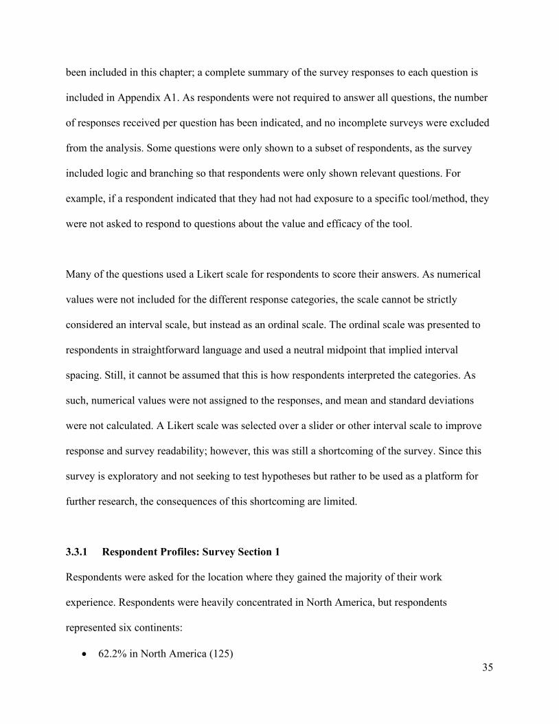
35

been included in this chapter; a complete summary of the survey responses to each question is

included in Appendix A1. As respondents were not required to answer all questions, the number

of responses received per question has been indicated, and no incomplete surveys were excluded

from the analysis. Some questions were only shown to a subset of respondents, as the survey

included logic and branching so that respondents were only shown relevant questions. For

example, if a respondent indicated that they had not had exposure to a specific tool/method, they

were not asked to respond to questions about the value and efficacy of the tool.

Many of the questions used a Likert scale for respondents to score their answers. As numerical

values were not included for the different response categories, the scale cannot be strictly

considered an interval scale, but instead as an ordinal scale. The ordinal scale was presented to

respondents in straightforward language and used a neutral midpoint that implied interval

spacing. Still, it cannot be assumed that this is how respondents interpreted the categories. As

such, numerical values were not assigned to the responses, and mean and standard deviations

were not calculated. A Likert scale was selected over a slider or other interval scale to improve

response and survey readability; however, this was still a shortcoming of the survey. Since this

survey is exploratory and not seeking to test hypotheses but rather to be used as a platform for

further research, the consequences of this shortcoming are limited.

3.3.1 Respondent Profiles: Survey Section 1

Respondents were asked for the location where they gained the majority of their work

experience. Respondents were heavily concentrated in North America, but respondents

represented six continents:

• 62.2% in North America (125)

36

• 16.9% in South America (34)

• 2.0% in Europe (4)

• 1.0% in Asia (2)

• 13.4% in Africa (27)

• 4.5% in Australia/Oceania (9)

Respondents were asked to identify their level of education; 84.1% of respondents have

completed a university degree, with 58% of respondents indicating that their professional or

technical training was in engineering fields. The level of education and discipline of study is

included in Table 3.1.

Table 3.1 Level and area of survey respondent education

Q1.3: What is the highest level of education you have completed? (If currently enrolled, highest degree received.)

Count %

Some secondary school, no graduation 2 1.0% Secondary school graduate 2 1.0% Some university credit, no degree 5 2.5% Trade/technical/vocational training 8 4.0% Associate degree or diploma 15 7.5% Bachelor's degree 101 50.3% Master's degree 63 31.3% Doctorate degree 5 2.5% Total 201

Q1.4: In what area is your professional or technical training? Count % Engineering 116 58.0% Geology 12 6.0% Business/Finance/Economics 36 18.0% Other Sciences 2 1.0% Arts/Humanities 3 1.5% Technical/Trades 12 6.0% Other 19 9.5% Total 200

Other questions regarding the respondents’ profiles include their level of experience, type of

company worked for, and stage of project experience. Mining companies and

engineering/technical consulting firms were the most represented companies, with a combined

37

84% of respondents. The level of project experience and typical roles on project teams was

broadly spread among seniority levels, with management levels (Functional/Area Managers,

Project Managers/Directors, Project Sponsors) forming 49.5% of respondents. The summary of

company type, respondent roles, and level of experience is included in Table 3.2. The respondent

profile data shows that 63% of survey respondents work in supervisory or managerial roles on

projects, and 58% of respondents have greater than years of work experience.

Table 3.2 Type of company and typical role/position

Q1.2: Your experience is primarily with which type of company: Count % Mining company (exploration, project development, or mining operations) 106 52.7% Engineering/technical consulting 63 31.3% Construction contractor or field services contractor 12 6.0% Equipment/material supplier 4 2.0% Other professional services (accounting, law, management consulting, etc.) 11 5.5% Other (please indicate) 5 2.5% Total 201

Q1.10: What is your typical role on project teams? Count % Project support from corporate/operations function (not full-time on a project) 35 17.5% Functional project role (engineer, designer, purchasing agent, etc.) 39 19.5% Discipline Lead 27 13.5% Functional/Area Manager 34 17.0% Project Manager/Director 54 27.0% Project Sponsor 11 5.5% Total 200

Q1.7: How many years of work experience do you have? Count % 0-5 2 1.0% 6-10 18 9.0% 11-15 35 17.5% 16-20 30 15.0% 21-25 34 17.0% 26-30 21 10.5% 31+ 60 30.0% Total 200

3.3.2 Exposure to Project Risk Management: Survey Section 2

Section 2 of the survey sought to identify the self-assessed level of project risk management

knowledge and whether the respondents had received any education or training in risk

38

management. This section also asked questions about the company's project risk management

policies/standards in which they worked. Respondents ranked themselves highly on self-

perceived knowledge of project risk, with 50.2% rating their knowledge as very or extremely

knowledgeable. 89% of respondents indicated that they had received some form of education and

training in project risk management, with 62% indicating informal professional development and

27% receiving formal professional development or formal education. These results are

summarized in Table 3.3

Table 3.3 Crosstab of risk knowledge and risk management training/education

Q2.1: How would you describe your overall knowledge of project risk management?

Risk Knowledge (Q2.1) Count % Education/Training (Q2.2)

None Informal PD Formal PD Education Not knowledgeable at all 2 1.0% 2 0 0 0 Slightly knowledgeable 8 4.0% 5 3 0 0 Moderately knowledgeable 90 44.8% 11 64 13 2 Very knowledgeable 80 39.8% 4 47 23 6 Extremely knowledgeable 21 10.4% 1 9 6 5

Total 201 23 123 42 13 Q2.2: Have you taken any training or education in risk management? (Included in the columns of the crosstab table)

“No training or education in risk management.” (None) “Informal training program (workshop, workplace training, on the job training.)” (Informal PD) “Formal professional development (multi-day course, professional certification.)” (Formal PD) “Formal educational program (degree, diploma, certificate.)” (Education)

As shown in Table 3.4, a large majority of respondents (75.1%) indicated that their companies

had written documentation of project risk management, with large numbers of people indicating

that companies had formal policies, standards, and procedures governing the application of

project risk management. This is a strong result indicating that many of the respondents likely

come from larger organizations with more conventional approaches to project risk management.

The self-assessed level of knowledge on these company documents is also high, with 50.7%

39

indicating that they are very or extremely knowledgeable and 40.5% answering as moderately

knowledgeable.

Table 3.4: Level of knowledge of company documentation on project risk management

Q2.4: Does your company have written documentation on project risk management? (e.g. policies, procedures, standards, guidelines, etc.)

Count %

Yes 151 75.1% No 38 18.9% I don't know 12 6.0% Total 201

Q2.5: What types of project risk management documentation exist within your organization? Please check all that apply. (n=146)

Count %

Company policies 103 70.5% Company standards 110 75.3% Procedures or guidelines 128 87.7% Training documentation 67 45.9% Project-specific guidelines/procedures 99 67.8% Informal documentation (PowerPoint presentations, emails, etc.) 86 58.9%

Note: Percentages is for the number of respondents that indicated their company had each type of documents; respondents were able to select multiple responses. Only respondents who answered “Yes” to Q2.4 were shown this question. Q2.6 How would you describe your level of knowledge of this project risk management documentation?

Count %

Not knowledgeable at all 1 0.7% Slightly knowledgeable 12 8.1% Moderately knowledgeable 60 40.5% Very knowledgeable 66 44.6% Extremely knowledgeable 9 6.1% Total 148

3.3.3 Definitions of Risk: Survey Section 3

Section 3 of the survey included three questions focused on the definitions of risk. Respondents

were asked to select their preferred definition of risk and whether they believed risk impacts

were negative, positive, or both. The motivation behind these questions was to determine how

respondents understood the concept and nature of risk. The definitions used for question Q3.1

were selected from a range of the most common definitions, including the expected loss

40

definition of risk (the product of probability and impact), the ISO definition, and one of the

suggested SRA definitions of risk. The AACEI and PMI definitions of risk were omitted, as their

definitions are essentially interchangeable with the ISO definition of risk, albeit the ISO

definition is not specific to project management. Since these definitions use “projects” in the

language, it was felt that these definitions would bias respondents’ selections. As shown in Table

3.5, most respondents (61.9%) selected the expected loss definition of risk. This definition of risk

is standard in quantitative techniques used in engineering, potentially explaining why it was the

most preferred definition. The remaining respondents were evenly distributed between the other

three definitions, with a small number selecting “other” definitions that they provided. A follow-

up question to the definition sought to understand how rigid or strong the belief in this definition

was and other definitions that respondents believed to be correct. 12.3% of respondents indicated

that there is only one definition of risk, 57% indicated that there are several possible definitions,

but the definition they selected was best, and 30% indicating that there are several definitions of

risk that are equally suitable. This result indicated the perceived flexibility in the definition of

risk. Further research should seek to determine if the flexibility in the definition is context-

specific and if respondents feel that different understanding or definitions of risk are suitable for

different applications or techniques in project risk management settings.

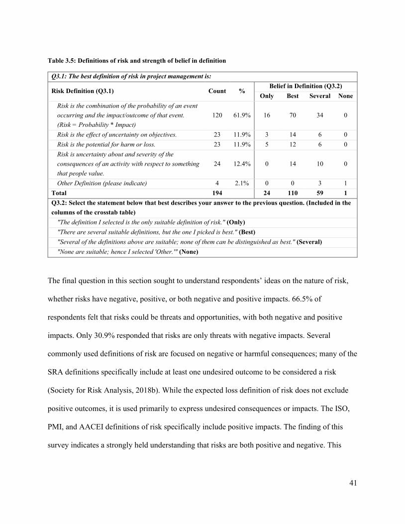
41

Table 3.5: Definitions of risk and strength of belief in definition

Q3.1: The best definition of risk in project management is:

Risk Definition (Q3.1) Count % Belief in Definition (Q3.2)

Only Best Several None Risk is the combination of the probability of an event occurring and the impact/outcome of that event. (Risk = Probability * Impact)

120 61.9% 16 70 34 0

Risk is the effect of uncertainty on objectives. 23 11.9% 3 14 6 0 Risk is the potential for harm or loss. 23 11.9% 5 12 6 0 Risk is uncertainty about and severity of the consequences of an activity with respect to something that people value.

24 12.4% 0 14 10 0

Other Definition (please indicate) 4 2.1% 0 0 3 1 Total 194 24 110 59 1 Q3.2: Select the statement below that best describes your answer to the previous question. (Included in the columns of the crosstab table)

"The definition I selected is the only suitable definition of risk." (Only) "There are several suitable definitions, but the one I picked is best." (Best) "Several of the definitions above are suitable; none of them can be distinguished as best." (Several) "None are suitable; hence I selected 'Other.'" (None)

The final question in this section sought to understand respondents’ ideas on the nature of risk,

whether risks have negative, positive, or both negative and positive impacts. 66.5% of

respondents felt that risks could be threats and opportunities, with both negative and positive

impacts. Only 30.9% responded that risks are only threats with negative impacts. Several

commonly used definitions of risk are focused on negative or harmful consequences; many of the

SRA definitions specifically include at least one undesired outcome to be considered a risk

(Society for Risk Analysis, 2018b). While the expected loss definition of risk does not exclude

positive outcomes, it is used primarily to express undesired consequences or impacts. The ISO,

PMI, and AACEI definitions of risk specifically include positive impacts. The finding of this

survey indicates a strongly held understanding that risks are both positive and negative. This

42

result could be due to the increased acceptance and adoption of approaches recommended by

standards organizations and professional associations.

Table 3.6: Views on the nature of risks in project management

Q3.3: What is your view on the nature of risks in project management? Count % Risks are potential threats; the impacts of risks occurring are negative. 60 30.9% Risks are potential opportunities; the impacts of risks occurring are positive. 0 0.00% Risks can be both potential threats or opportunities; the impacts of risks occurring can be both positive or negative.

129 66.5%

Other (please indicate) 5 2.6% Total 194

3.3.4 Use and Perception of Risk Management Tools: Survey Section 4

Section 4 sought to identify what tools and methods are being used to manage risks and the

perceived value and efficacy of these tools. Table 3.7 summarizes the respondents' views on the

efficacy of project risk assessments in achieving the process objectives (satisfying the steps

required to complete a risk assessment) of project risk assessments. There are two insights of

interest from these results. Firstly, less than 50% of respondents scored accurate quantification of

the probability and impacts of risk as “very effective” or “extremely effective.” Secondly, 50%-

77% of respondents scored the remaining five process objectives as “very effective” or

“extremely effective.” Overall, this indicates that respondents largely believe that risk

assessments effectively achieve their aims, although risk quantification is viewed as less

effective than other risk assessment activities.

43

Table 3.7: Belief in project risk assessment effectiveness

Q4.3 - Do you believe that project risks assessments are effective in the following: Not Slightly Moderately Very Extremely Total Identifying a comprehensive list of risks

0.00% 2.17% 21.20% 56.52% 20.11% 184

Accurately identifying the causes of risks

0.55% 7.65% 43.17% 40.98% 7.65% 183

Accurately quantifying the probability of risks occurring

2.72% 20.65% 46.20% 25.54% 4.89% 184

Accurately identifying possible risk impacts

1.10% 6.04% 43.41% 41.76% 7.69% 182

Accurately quantifying risk impacts

3.83% 14.75% 46.99% 27.32% 7.10% 183

Accurately ranking and prioritizing risks

0.55% 9.34% 32.97% 42.86% 14.29% 182

Developing useful risk response plans

1.65% 12.64% 31.87% 39.56% 14.29% 182

Tables 3.8 and 3.9 show the results from questions asking respondents which tools/methods they

have used in risk assessments and their attitudes on the effectiveness of these tools. Responses

indicate that risk matrices, risk registers, HAZOP Studies, and Monte Carlo simulations are the

most commonly used tools. More sophisticated and specialized tools, such as Failure Mode and

Effects Analysis (FMEA), were less used by respondents. The most interesting result from the

perceived effectiveness of these tools is that for the four most commonly used tools listed above,

68.2% considered Monte Carlo simulations the least effective, while 77.7% considered HAZOP

studies the most effective. These results are consistent with the results shown in Table 3.7. Some

investigation may be required to determine why simulations are considered less effective than

other tools in helping characterize and assess risk.

44

Table 3.8 Use of project risk management tools and methods

Q4.4: Which of the following risk management tools/methods have you used in a project risk assessment? (n=182)

Count %

Risk Matrices 154 84.6% Risk Registers 150 82.4% Hazard and Operability Studies (HAZOP) 124 68.1% Monte Carlo Simulations 112 61.5% PERT Schedule Analysis 63 34.6% Failure Mode and Effects Analysis (FMEA) 53 29.1% Risk Bowtie Analysis 53 29.1% Fault Tree Analysis (FTA) 37 20.3% Event Tree Analysis (ETA) 30 16.5% Risk Data Quality Assessments 19 10.4% Delphi Technique 11 6.0% Vulnerability Analysis 9 4.9%

Note: Percent indicated is the percentage of the 182 respondents to this question who have used the tool/method.

Table 3.9 Perceived effectiveness of project risk management tools and methods

Q4.6: In your opinion, how effective are these tools/methods at helping assess and manage project risks: Not Slightly Moderately Very Extremely Total Risk Matrices 0.0% 8.7% 34.7% 41.3% 15.3% 150 Risk Registers 2.1% 8.9% 32.9% 37.7% 18.5% 146 Hazard and Operability Studies (HAZOP)

0.0% 1.7% 20.7% 50.4% 27.3% 121

Monte Carlo Simulations 3.6% 15.5% 49.1% 22.7% 9.1% 110 PERT Schedule Analysis 0.0% 9.8% 37.7% 45.9% 6.6% 61 Failure Mode and Effects Analysis (FMEA)

1.9% 13.2% 43.4% 35.9% 5.7% 53

Risk Bowtie Analysis 0.0% 11.5% 30.8% 53.9% 3.9% 52 Fault Tree Analysis (FTA) 0.0% 22.2% 44.4% 30.6% 2.8% 36 Event Tree Analysis (ETA) 0.0% 31.0% 41.4% 24.1% 3.5% 29 Risk Data Quality Assessments 0.0% 0.0% 44.4% 44.4% 11.1% 18 Delphi Technique 0.0% 0.0% 36.4% 45.5% 18.2% 11 Vulnerability Analysis 0.0% 12.5% 62.5% 25.0% 0.0% 8

Tables 3.1 and 3.11 summarize the results from the questions regarding methods used to analyze

the probability of risk occurrence and the perceived effectiveness of these tools. Most

respondents (84.4%) have used qualitative ordinal scales (low/medium/high) to assess

45

probability, which is also the most common method. Fewer respondents indicate using single-

point estimates than multiple-point estimates and ranges, which is surprising as using multiple-

point estimates and ranges is considered a more sophisticated technique. This may result from

the question phrasing or descriptors provided or from the definition of single and multiple point

estimates. Only 31.7% of respondents report having used probability distributions to analyze the

probability of risk occurrence. Again, this lower number may be due to confusion caused by the

phrasing of the survey questions, as there is overlap between the categories of “multiple point

estimates and probability ranges” and “probability distributions” (e.g. uniform and triangular

distributions could have been interpreted as belonging in either category based on the

descriptions provided.) When assessing the efficacy of these approaches, respondents indicate

that the more sophisticated probability modelling techniques, such as multiple-point estimates,

probability distributions, and imprecise ranges, are more effective at helping understand and

analyzing probability. This result is consistent with the open-ended questions discussed later in

this chapter that more advanced techniques to quantify risk are necessary.

Table 3.10 Use of probability modelling techniques in project risk assessments

Q4.7: What methods have you have used to analyze the probability of risk occurrence? (n=186)

Count %

Qualitative classification (e.g. low, medium, high) 157 84.4% Single point estimates (e.g. average, median, or expected values) 67 36.0% Multiple point estimates or probability ranges (e.g. maximum, minimum, and most likely)

110 59.1%

Probability distributions (e.g. probability density functions, cumulative probability distributions)

59 31.7%

Overlapping or imprecise ranges/distributions (e.g. fuzzy sets or possibility intervals) 11 5.9% Note: Percent indicated is the percentage of the 186 respondents to this question who have used the tool/method identified.

46

Table 3.11 Perceptions of effectiveness of probability modelling techniques

Q4.8 - How effective are these methods in helping understand and analyze the uncertainty associated with risks? (Same methods as listed in Q4.7)

Not Slightly Moderately Very Extremely Total Qualitative classification 2.0% 13.7% 45.8% 31.4% 7.2% 153 Single point estimates 7.5% 15.0% 64.2% 10.5% 3.0% 67 Multiple point estimates or probability ranges

0.0% 6.4% 42.2% 42.2% 9.2% 109

Probability distributions 1.7% 8.5% 23.7% 54.2% 11.9% 59 Overlapping or imprecise ranges/distributions

0.0% 18.2% 27.3% 36.6% 18.2% 11

The final questions in section 4 of the survey sought to determine respondents’ perceptions on

risk ranking and prioritization through qualitative and quantitative methods; the results of these

questions are included in Table 3.12. Responses indicate that respondents feel equally strongly

that qualitative and quantitative methods effectively rank and prioritize risk. This may appear

counterintuitive compared to previous questions, where respondents indicated that qualitative

methods were less effective at understanding and analyzing uncertainty. However, this could be

explained as respondents feeling that quantitative methods produce more accurate risk analyses

to quantify probability and impact, but qualitative methods can still correctly rank and prioritize

risks. This possible explanation could be explored in further research to determine the causes or

reasons for the perceived effectiveness of qualitative assessments for risk ranking and

prioritization. In the final question, respondents indicated less confidence in accurately analyzing

rare and catastrophic risks through quantitative probability and impact assessments. The reasons

for this must also be explored, but a possible explanation is that when probabilities are extremely

low, and impacts are very high, it is possible to make significant estimation errors for probability

and impact. The lack of relevant historical data for rare events may further challenge accurate

quantification. The difference of probability assessment between 0.001 and 0.0001 may not be

47

practically understood or appreciated by those doing the risk assessment, yet the resultant

expected loss calculations will differ by an order of magnitude.

Table 3.12 Perceptions on the effectiveness of risk ranking and prioritization methods

Q4.10: Do you agree or disagree that combining probability and impact in a Risk Matrix to get a qualitative risk classification results in accurately ranked and prioritized risks?

Count %

Strongly disagree 2 1.1% Somewhat disagree 20 10.8% Neither agree nor disagree 19 10.2% Somewhat agree 120 64.5% Strongly agree 25 13.4% Total 186

Q4.11: Do you agree or disagree that expressing risk as a combination of probability and impact (risk = probability * impact) results in accurately ranked and prioritized risks?

Count %


Q4.12: Do you agree or disagree that expressing risk as a combination of probability and impact (risk = probability * impact) is adequate to analyze project risks with very low probabilities and extremely high impacts? (e.g. security/terrorism risks, catastrophic natural disasters, etc.)

Count %


3.3.5 The Risk Concept and New Perspectives on Risk: Survey Section 5

Section 5 of the survey sought to explore respondents’ perceptions on some of the concepts of

the new perspectives on risk discussed earlier in this dissertation. Table 3.13 summarizes the

responses to questions about the prevalence of unexpected and unforeseen risks. Respondents

48

report that unexpected and unforeseen risks - risks that were not identified in advance in a risk

assessment exercise - occur in less than half of projects. This result is surprising as it indicates

that respondents either feel that risk assessments are sufficiently effective in identifying risk such

that unforeseen risks occur in a minority of projects or that unforeseen risks are by nature rare

enough to occur in a minority of projects. Another possibility is that respondents applied a

materiality filter in answering this question, so they only considered unforeseen risks with

significant impacts in their responses, which would be less rare. Respondents were largely

neutral of the effectiveness of standard project risk management methods in managing

unforeseen and unexpected risks, with 57.5% indicating these methods are moderately effective.

Table 3.13 Perceptions on unexpected and unforeseen risks

Q5.1: In your experience in mining projects, how frequently do unexpected or unforeseen risks emerge during the project that were not previously identified in a risk assessment?

Count %

Never 0 0.0% Sometimes 81 44.0% About half the time 54 29.4% Most of the time 49 26.6% Always 0 0.0% Total 184

Q5.2: How effective are the project risk management methods you've used in helping manage these unexpected and unforeseen risks?

Count %

Not effective at all 9 4.97% Slightly effective 20 11.05% Moderately effective 104 57.46% Very effective 44 24.31% Extremely effective 4 2.21% Total 181

Table 3.14 summarizes the responses on definitions of uncertainty and probability in project risk

management and how strongly respondents believe in their preferred definition. Two of the most

common definitions of uncertainty and probability were adapted from the literature for these

49

questions. The question on uncertainty provides simplified definitions for aleatory and epistemic

uncertainty. Aleatory uncertainty is defined as variability and lack of predictability and epistemic

uncertainty defined as a lack of knowledge. Respondents are nearly even on their definitions,

with 51.4% selecting the definition aligned with aleatory uncertainty and 44.8% selecting the

epistemic uncertainty definition. When asked about the strength of belief in their preferred

definition, 21% indicated their response was the only suitable definition, 55% indicated that both

definitions were suitable, but their preferred definition was better, and 22% indicated that both

were equally suitable definitions.

Table 3.14 Definition of uncertainty in project risk management

Q5.7: In project risk management, uncertainty is best described as:

Uncertainty Definition (Q5.7) Count % Belief in Definition (Q5.8)

Only Best Both Neither The variability and lack of predictability in project parameters (cost, activity duration, performance variables, etc.)

93 51.4% 20 58 15 0

The lack of knowledge about the causes, likelihood, and consequences of possible future events.

81 44.8% 18 41 22 0

Other (Please indicate) 7 3.9% 0 1 2 4 Total 181 38 100 39 4 Q5.8: Choose the statement below that best describes your answer to the previous question. (Included in the columns of the crosstab table)

The statement I selected is the only suitable definition. (Only) Both are suitable definitions, but the one I picked is best. (Best) Both definitions are equally suitable; neither is better. (Both) Neither are suitable; hence I selected "Other." (None)

Table 3.15 shows the questions asking respondents for their definitions of probability in a project

risk management context. The responses included definitions of probability that represented

frequentist and subjective probabilities. A majority (61.3%) selected the subjective probability

definition, identifying that probability in project risk management is best described as a degree-

50

of-belief instead of a statistical interpretation of probability. This is somewhat surprising and

seems to contrast with the preferred definition of uncertainty, for which respondents favoured the

aleatory or statistical interpretation of uncertainty over epistemic uncertainty. This may be due to

the respondents’ experience with project risk assessments. The probabilities assigned to threats,

hazards, and other risk scenarios are often based on expert judgment rather than historical data.

Respondents may have had more exposure to this definition and believe it favourable in a project

context. Respondents had slightly more strength of belief in their preferred definition, with

24.9% indicating that their selected answer was the only suitable answer, 56.4% indicating that

both answers were suitable, but their selected answer was best, and 16% indicating that both

responses were equally acceptable.

Table 3.15 Definition of probability in project risk management

Q5.9: In project risk assessments, probability is best described as:

Probability Definition (Q5.9) Count % Belief in Definition (Q5.10)

Only Best Both Neither The relative frequency of an event occurring (how often it occurs divided by all possible outcomes, based on historical data, sampling, etc.)

62 34.3% 18 39 5 0

The degree of belief of whether an event will occur (based on expert judgement, predictive models, etc.)

111 61.3% 27 62 22 0

Other (please indicate) 8 4.4% 0 1 2 5 Total 181 45 102 29 5 Q5.10: Select the statement below that best describes your answer to the previous question. (Included in the columns of the crosstab table)

The statement I selected is the only suitable definition. (Only) Both are suitable definitions, but the one I picked is best. (Best) Both definitions are equally suitable; neither is better. (Both) Neither are suitable; hence I selected "Other." (None)

The concept of strength of knowledge was introduced and defined in the survey, as shown

below. The definition and purpose for considering strength of knowledge in risk assessments

51

were provided as it is not commonly used. The text in the survey defining strength of knowledge

is as follows:

“Some researchers in the field of risk analysis have suggested that knowledge should be accepted as risk characteristic and should be specifically included in risk assessments to improve our understanding about risks. Knowledge about a risk helps inform and condition our assessments of probability, potential consequences, and the uncertainty that underlies the risk. Assessing strength of knowledge could be used to qualify or validate the other dimensions of the risk assessment. This improved analysis could ultimately lead to better risk response planning and decision making.”

Table 3.16 shows that only 26.4% of respondents indicated they had been exposed to the concept

of strength of knowledge in a risk assessment. 18.1% indicated that they have specifically

assessed strength of knowledge in a project risk assessment. Respondents were not questioned on

how this strength of knowledge assessment was performed, the ranking or metrics used, or how

it was incorporated into the overall risk assessment. These are areas of potential further

investigation.

Although familiarity and use of strength of knowledge assessments were low, 84.6% of

respondents indicated they either somewhat agreed or strongly agreed that it would improve risk

assessments. When questioned about the potential for strength of knowledge relative to a risk to

change over time, 89.5% agreed that strength of knowledge assessments are fluid and can

change. This is perhaps an obvious result, as knowledge can be improved through observation,

experimentation, or other information-gathering activities. Knowledge can also decrease if

changing conditions or uncertainties underlying the risk change, especially if the risk in question

is not a static exogenous phenomenon. When managing risks with opposing intelligent actors,

52

such as social or community relations risk, or permitting and regulatory risks, strength of

knowledge may be more dynamic than for many technical risks.

Table 3.16 Perceptions on including strength of knowledge in risk assessments

Q5.12: Have you ever been exposed to the concept of strength of knowledge in project risk assessments?

Count %


Q5.13: Have you ever specifically assessed strength of knowledge in a project risk assessment?

Count %


Q5.14: Do you agree or disagree that assessing strength of knowledge would improve project risk assessments?

Count %


Q5.15: Do you agree or disagree that strength of knowledge is fluid and can change over time?

Count %


3.4 Open-Ended Results and Analysis: Survey Section 6

The open-ended portion of the survey included four questions allowing respondents to comment

on their perceptions of project risk management strengths, weaknesses, challenges, and

improvements. The qualitative survey data was imported into NVivo, a qualitative data analysis

53

software package, to code and analyze the results. This allowed individual respondent comments

to be coded according to various topics and themes of interest. Details on the coding structures

used are included in the following sections.

3.4.1 Strengths of Project Risk Management

Questions Q6.1 of the open-ended portion of the survey asked respondents to comment on the

perceived strengths of project risk management. The question was written as follows:

Q6.1: What are the greatest strengths of project risk management?

Survey respondents provided 150 individual responses for this question. The response comments

were grouped into common topics and then were grouped into four major themes. Table 3.17

shows the topics and themes with the number of comments per topic; a summary and discussion

of major themes are included following the table. The number of responses coded to each topic

does not add up to the total number of responses received, as some responses included multiple

comments coded to different topics.

Table 3.17 Survey response topics grouped by major theme (question Q6.1)

T1: Building Risk Awareness: 97 Comments T2: Better Understanding Risks 41 Comments Risk Identification: 43 Comments Risk Awareness/Communication: 34 Comments Formal and Structured Process: 20 Comments

Harnessing Experience/Knowledge: 17 Comments Risk Analysis and Quantification: 11 Comments Risk Ranking and Prioritization: 11 Comments Risk Appetite and Tolerance: 2 Comments

T3: A Platform for Action: 61 Comments T4: Improving Project Outcomes: 34 Comments Risk Control and Mitigation: 59 Comments Risk Monitoring: 2 Comments

Improving Project Success: 19 Comments Improved Contingency Allocation: 13 Comments Improved Decision Making: 2 Comments

54

3.4.1.1 Theme #1 (T1): Building Risk Awareness

Many survey respondents credited project risk management programs with creating awareness of

risks and providing a forum for discussing and communicating about project risks. From the

comments, some respondents consider improved awareness and communication to be a central

feature or benefit of the risk management process; fostering discussions about risk will

inherently lead to better risk management actions and improved project outcomes. While it is

doubtful that increased awareness alone can improve risk management outcomes, it is likely that

increased awareness - being the necessary first step of a comprehensive risk management

program - might be a required step to improved risk management outcomes.

Many respondents felt that risk management procedures and methods provided more structure to

identify and assess risks and helps creates a risk management mindset within the project. The

formal process allowed teams to better identify risks and effectively reduce unwanted surprises

or improve management response to risk.

3.4.1.2 Theme #2 (T2): Better Understanding Risks

Many survey respondents indicated that one of the greatest strengths of project risk management

programs was that they led to an improved understanding through risk assessments and

characterizations. Consequently, risk responses and risk management outcomes are improved.

The improved understanding of project risks included three aspects. Firstly, that respondents felt

they had a more complete view of the project risk landscape. Secondly, they could quantify and

characterize individual risks by following the risk management process. Thirdly, that better

understanding and assessment of risks led to more reliable ranking and risk prioritization.

Respondents also indicated that the risk assessment process elicited valuable insight based on

55

team member experience and knowledge. This knowledge may not have been shared or drawn

out without the risk management program. Interestingly, only two responses included mention of

risk tolerance, which indicates that this significant aspect of risk management may be

insufficiently addressed in many risk management programs.

3.4.1.3 Theme #3 (T3): A Platform for Action

A large number of comments indicated that a critical strength of project risk management

programs is their ability to drive the implementation of risk management actions. Risk response

and risk control planning is a feature of virtually all risk management processes and frameworks.

It was felt that identifying controls and actions increased the quality and confidence in those

actions and distinctly improved follow-through and implementation. Several respondents

indicated that efforts to identify personal responsibility also increased follow-through.

3.4.1.4 Theme #4 (T4): Improving Project Outcomes

A smaller number of survey respondents identified the improved project outcomes rather than

risk management processes as the greatest strength of project risk management. Interestingly,

when asked about the greatest strength of project risk management, most people did not respond

with some version of “it improves project success” or “it reduces negative impacts of risks.” This

is perhaps a sign of the challenges faced in designing and implementing strong project risk

management programs; many project team members do not explicitly and instinctively connect it

with improved project outcomes. Instead, they focus on the process benefits, such as improved

awareness, communication, and understanding of risks. The respondents who indicated that

improved project outcomes were the greatest strength described improved decision-making

processes and increased confidence in decisions as strengths. Some respondents indicated that

56

budget and schedule performance was improved, while others focused on the risk management

process providing inputs to cost and schedule contingency allocation. Several comments

indicated that a quantitatively rigorous risk management program could increase confidence in

the accuracy of cost and schedule estimates and contingency allocations.

3.4.2 Weaknesses, Challenges, and Improvements

Questions Q6.2, Q6.3, and Q6.4 of the open-ended portion of the survey asked respondents to

provide comments on what they believed were the weaknesses, challenges, and improvements to

project risk management. The three questions included were as follows:

Q6.2: What are the greatest weaknesses of project risk management? Q6.3: What are the greatest challenges you've faced in implementing an effective

project risk management program? Q6.4: What improvements to project risk management tools, methods, or processes

would be the most beneficial?

In total, 435 individual responses were received from the survey respondents for the three

questions. These response comments were classified into different topics and then were grouped

into eight major themes across the three questions. The themes were grouped across the three

questions as many of the responses included considerable overlap, and the suggested

improvements followed from the weaknesses and challenges. Table 3.18 summarizes all the

response topics and themes in survey questions Q6.2, Q6.3, and Q6.4. A summary and

discussion of the major themes are included following the results table. The number of responses

coded to each topic does not add to the total responses received for each question. Some

responses included multiple comments coded to different topics.

57

Table 3.18 Survey response topics grouped by major theme (questions Q6.2, Q6.3, Q6.4)

T1: Accuracy and Completeness: 155 Comments T2: Support and Participation: 129 Comments Inaccurate Quantification and Prioritization (Q6.2): 29 Comments Cannot Identify all Risks (Q6.2): 23 Comments Better Analysis and Quantification Methods (Q6.4): 23 Comments Inaccurate Quantification Characterization (Q6.3): 13 Comments Political and Strategic Bias, Group Dynamics (Q6.2): 12 Comments Thoroughness of Risk Analysis Assessment (Q6.3): 12 Comments Subjectivity in Risk Assessments (Q6.2): 10 Comments Use and Acceptance of Data/Facts (Q6.4): 8 Comments Bias or Conflict in Proper Risk Assessments (Q6.3): 7 Comments Lack of Reliable Data for Risk Analysis (Q6.2): 5 Comments More Comprehensive Risk Identification (Q6.4): 5 Comments Limited View of Risk Landscape (Q6.2): 5 Comments Risk Response Planning is Superficial (Q6.2): 2 Comments Analysis of Risk Causes (Q6.2): 1 Comment

Gaining Management Buy-In and Support (Q6.3): 38 Comments Lack of Management Support and Participation (Q6.2): 22 Comments Effective Engagement and Participation (Q6.3): 17 Comments Inadequate Time or Resources (Q6.3): 15 Comments Reduce Project Silos / Increased Participation (Q6.4): 8 Comments Management Support and Commitment (Q6.4): 7 Comments Dedicated Resources (People, Time, Money) (Q6.4): 7 Comments Not Integrated into Project Management (Q6.3): 7 Comments Risk Communication (Q6.3): 3 Comments Not Integrated into Project Management (Q6.2): 3 Comments Better Communications of Risk Value (ROI) (Q6.4): 2 Comments

T3: Improving Follow-Through: 85 Comments T4: Knowledge and Training: 84 Comments Lack of Cohesive and Coordinated Follow-Up (Q6.3): 23 Comments Propper Monitor and Control Follow-Up (Q6.3): 20 Comments Poor Monitoring and Control Follow-Up (Q6.2): 12 Comments Making it an Ongoing Process (Q6.4): 12 Comments Intermittent and Infrequent Process (Q6.2): 10 Comments Ensuring Mitigations and Controls are Implemented (Q6.4): 8 Comments

Lack of Participant Knowledge and Expertise (Q6.2): 36 Comments More Training and Education (Q6.4): 22 Comments Understanding of Risk and RM Processes (Q6.3): 20 Comments Experienced and Knowledgeable Participants (Q6.4): 6 Comments

T5: Fit for Purpose / Consistency: 44 Comments T6: From Compliance to Value-Add: 23 Comments Fit for Purpose / Simple and Efficient Methods (Q6.4): 25 Comments Arduous and Complicated Process (Q6.2): 13 Comments Inconsistent Application of RM Practices (Q6.2): 6 Comments

Satisfying a Requirement / Checkbox Exercise (Q6.2): 11 Comments Satisfying a Requirement / Checkbox Exercise (Q6.3): 9 Comments Not Aligned to Business Strategy (Q6.2): 2 Comments No Focus on Opportunities (Q6.2): 1 Comment

T7: Tools, Methods, and Systems: 13 Comments T8: Quality and Improvement: 9 Comments Better Systems and Technology (Q6.4): 13 Comments Formalized Lessons Learned or Review Procedures (Q6.4): 6 Comments

Include High-Level Peer Review (Q6.4): 3 Comments

58

3.4.2.1 Theme #1 (T1): Improving Risk Assessment Accuracy and Completeness

The largest area of comments from the survey respondents related to the perceived accuracy and

completeness of the risk assessments and the risk management process. This theme included

several topics relating to risk identification, risk analysis and characterization, and risk

responses.

Survey respondents’ comments indicated that the risk identification process is often done quickly

and lacks thoroughness, leading to an incomplete list of risks. The identified risks are the most

obvious or common ones in many mining projects (community opposition, slow permitting

process, construction productivity, etc.) The risk identification process often does not follow a

highly structured or systematic process, which leads to large numbers or broad categories of risks

being inadvertently omitted. There was a significant perception that not all risks can be identified

in advance or risks are known but have a negligible probability of occurrence, so they are not

included in the risk register.

Improper risk analysis and quantification was the most noted topic in the open-ended portion of

the survey. Many felt that risk assessments were too subjective, relied too heavily on opinion,

and were subject to individual biases and behaviours that biased group dynamics. When there

was relevant data available to use for risk analyses, it was not always adequately used. Many

ranking and prioritization methods use qualitative rankings, which do not always provide

sufficient or accurate detail. The lack of a rigorous, structured, and principled process of

quantifying risks left many respondents feeling that the process is too open to influence or

manipulation by participants with specific motives or desired outcomes.

59

Finally, survey respondents felt that the risk response planning involved in the risk assessment

exercises was often superficial and did not provide realistic or detailed plans for responding to

risks.

3.4.2.2 Theme #2 (T2): Gaining Management Support and Effective Participation

Insufficient active management support for risk management efforts was identified as a weakness

and challenge to implementing risk management programs. Respondents indicated that gaining

active management support and promotion was critical to building a risk management program.

Without management support, resources were not available to do the risk management work, and

participants were less likely to be fully engaged and participate in the process. Survey

respondents strongly indicated that this management support was an area for the Project Sponsor

to positively influence the risk management behaviours and outcomes. Project teams are much

more likely to embrace the risk management process if it has backing from the Project Sponsor

or Steering Committee.

Strong management support of risk management efforts leads to proper resource allocation for

the risk management program, including dedicated personnel to manage and coordinate risk

management efforts and the time commitment from project team members to participate in the

process. Failing to dedicate resources resulted in poorly managed programs with nobody

coordinating or championing the risk work. Survey respondents also strongly indicated that

participation and belief in the process from project team members was a challenge. Project team

members often feel that their involvement in the risk assessment and risk management process

was outside of their regular duties and not as important as their primary role. Ideas for improving

60

engagement and participation from team members included securing strong management support

and increased risk management training and education for project team members.

3.4.2.3 Theme #3 (T3): Improving Risk Management Follow-Through

Many of the survey respondents felt that the risk management exercises that they had

participated in were cursory, performed as part of project stage-gate requirements, and not

adequately carried forward or revisited throughout the remainder of the project. The reasons for

this lack of follow-through relate to other key themes in the survey findings: that the exercise

was viewed as a “check-box” exercise and was undertaken to comply with project procedures

and requirements, that it lacked proper management support, that there were inadequate

resources available to support an ongoing risk management program, and that participants

struggled to connect risk management efforts to improving project success or adding value.

Several respondents commented that risk response plans were not revisited, even when the risk

they were designed to manage and mitigate emerged. Many respondents suggested

improvements to increase the frequency of formal risk management interactions with the project

to turn the risk management efforts into a continuous and embedded feature of project

management. Others suggested that risk management programs should include verification and

compliance measures to ensure identified actions are implemented. Some respondents noted that

this level of risk management integration with the project was at odds with the desire for risk

management methods and systems to be fit-for-purpose, simple and understandable, and not

overly demanding to implement.

61

3.4.2.4 Theme #4 (T4): Improving Risk Management Knowledge and Training

A lack of knowledge and understanding of risk management tools and methods was identified as

a challenge and a potential area of improvement by survey respondents. Many respondents

commented that there is significant ambiguity and lack of cohesion on the concepts and

definitions of risk, and thus many different approaches for managing risks. Many risk

management professionals or participants follow their preferred way in the absence of clear

guidelines and procedures. The lack of cohesive definitions identified by respondents aligns with

the definitional debate described in Chapter 2. Many respondents commented that risk

management programs could be improved if companies developed and implemented clear,

formal, and consistent standards for project risk management and ensured project team members

had access to sufficient training. Some respondents commented that the multi-organizational

nature of projects, with project owners and several engineering or construction firms engaged on

a single project with their discrete scopes of work, created tension behind following a common

approach to risk management.

In addition to improving participants' knowledge, respondents also indicated that risk

management coordinators and facilitators needed to be experts in the theory, practice, and

implementation of risk management. Several respondents perceived that there were not many

strong project risk management practitioners and few genuinely skilled experts in this field.

3.4.2.5 Theme #5 (T5): Fit for Purpose and Consistent Application

Many survey respondents indicated that they wanted project risk management methods and tools

to be fit-for-purpose, meaning that they are suitable and flexible for different sizes and stages of

projects. There were differences in opinion among the survey respondents, with some feeling

62

that a simple and easy-to-understand approach would be best while others favoured a more

comprehensive, detailed, and time-consuming effort. Some respondents recognized the inherent

trade-off between the level of effort and the value of the results. However, many still indicated

that they wanted something “simple yet effective,” assuming that there is some undiscovered

solution that offers both and that there is a broadly acceptable definition or measure of both of

the terms “simple” and “effective.” Perhaps the underlying sentiments with comments of this

type are that respondents have taken part in project risk management approaches that have been

complicated and ineffective, requiring substantial effort but without the corresponding benefit. It

is clear that there is a desire for optimization of effort versus output where ease of

implementation and results are multiple objectives.

3.4.2.6 Theme #6 (T6): Moving from Compliance to Value-Add

Several survey respondents indicated that many of the project risk management efforts they had

previously been involved with felt like “check-box” exercises, implemented ostensibly to assess

and manage risk, but really to satisfy procedural requirements before a stage-gate review or

project audit. Several respondents suggested that project risk management programs' perceived

benefit does not justify the time and effort involved. The results are not reliable; hence the

process is not seriously accepted by many project team members. Some respondents commented

that reviews and audits should focus both on results achieved and whether or not procedures

were followed. The perceived usefulness relates to many other themes identified in the survey

responses; if participants believed that the results were accurate and complete, they would

believe more strongly in the project risk management value proposition.

63

3.4.2.7 Theme #7 (T7): Clarifying Tools, Methods, and Systems

These comments in this theme relate to the software, applications, and management information

systems used for project risk management. While the idea of improving the tools, methods, and

systems was not one of the most common themes, it relates to many of the other themes or

underpins the suggested improvements included in the other themes. The use of scalable systems

helps improve consistency and allows flexibility for different sizes and stages of projects.

Intuitive and easy-to-use systems will help improve follow-through. Analytically powerful

systems can help improve accuracy and completeness in risk quantification. Strong systems used

to support the risk management approach will build support and confidence in the results. Many

respondents commented that spreadsheets were used to manage and communicate risk

information and that risk registers often became large and cumbersome. Many also suggested

using automated database tools to help project team members manage their risks, improve

continuity of the risk management process, and communicate the status and progress of risk

management efforts.

3.4.2.8 Theme #8 (T8): Quality Assurance and Continual Improvement

A small number of survey respondents commented that project risk management practices

appeared to be missing quality assurance or peer reviews or subject to an audit process that

reviews the procedures and methods for project risk management. They commented that the peer

reviewers should review both the risk processes themselves and the risk assessments to check the

accuracy of the risk assessment. Perhaps this peer-review aspect has not been addressed in

practice because risk management is already seen as a type of peer review or quality review on

project design and execution plans. The final comment from respondents was that risk

management outputs from previous projects were not frequently used when initiating new

64

projects. The recommendation from this is that risk management outputs should become part of

project lessons learned programs, and the risk management program itself should be subject to a

lessons learned and continuous improvement review.

3.5 Conclusion

Based on the results of the multiple-choice and open-ended questions, survey respondents

indicated that they were broadly exposed to risk management practices, tools, and methods and

that they largely felt that these tools were effective in helping manage project risks. However,

these perceptions of effectiveness are subjective, and effectiveness was not purposefully defined.

A different and more pointed phrasing of the question, such as “do these methods achieve risk

management objectives?” or “do these methods reduce risk?” may have received different

results.

A summary-level interpretation of the results and themes presented in this chapter can suggest

that survey respondents want to improve risk management practices by improving analytical

techniques, improving the structure and process, and integrating risk programs deeper into the

project. An effective risk management program is continuous, consistent, and clear in its

methods and benefits. A project risk management program that is more seamlessly folded into

the daily workings of project teams, a type of “risk layer” that augments regular engineering and

project work, is one that seems to satisfy the desires of respondents. Similar approaches have

been taken with project value and quality management to infuse project work with their

respective principles, proving more effective than irregular and infrequent engagements with the

broader project.

65

Survey respondents responded favourably to elements of the new perspectives on risk,

recognizing the fluidity of many risk characteristics and the value in providing better

assessments of uncertainty underlying risks and the knowledge that conditions our risk

assessments. Specifically addressing and assessing these parameters in a risk assessment may

help strengthen both project risk analysis and project risk response. However, subjective survey

responses soliciting perceptions are only a first step. Additional research must investigate the

best methods to practically incorporate these new risk perspectives, then study their performance

to determine if new perspectives help improve risk management outcomes and reduce risks.

Respondents generally seemed to acknowledge the potential value of project risk management

and that more structure, consistency, and integration would help. Still, it also appears they

demand too much without the willingness to expend the effort to satisfy these demands.

Expecting methods to be “simple yet effective” may justify and excuse a lack of commitment to

pursuing rigorous methods that require substantial resources and effort.

One response, in particular, was emblematic of one of the many challenges faced in designing

and implementing project risk management programs:

“Need a way to capture unknown unknowns – events that cannot be predicted based on past frequency or expert judgement.”

This response is interesting in many ways, foremost in indicating the expectations mining project

professionals have of project risk management methods – they expect it to predict the unknown.

A sympathetic interpretation of this comment is that the respondent believes more rigour and

66

detail are required so more risks are identified and characterized, or perhaps that superficial

methods leave many significant risks undiscovered. Better risk management processes might

expand the space of what is known and knowable, leaving less potentially harmful risks

unidentified. This would be a worthy pursuit. However, a literal interpretation – that risk

assessment processes should capture novel events that are unknown and unknowable and cannot

be predicted by a group of experts – shows the headwinds faced by risk management

professionals. If not through previous experience or expert judgement, how would they be

identified? However, while it may be unrealistic to expect a risk assessment process to capture

and identify unknown and unknowable risks, it is possible to develop a risk management

program that is responsive, flexible, and adaptable to these emerging and highly uncertain risks.

This comment reinforces the motivation behind this research, as one such approach to manage

emerging risks is explored in the remainder of this dissertation.

67

Chapter 4: The Adaptive Project Risk Management Framework

4.1 Introduction

The adaptive project risk management framework presented in this dissertation includes two key

components: a process that describes the steps and requirements for the adaptive framework and

a system model that provides quantitative inputs to the decision process. The adaptive project

risk management framework is based on adaptive management and adaptive risk management

principles and is tailored to apply specifically to capital development projects.

This chapter includes a description of the adaptive framework and the detailed adaptive process.

It also includes a description of the key literature in adaptive management, discusses the

motivation for applying adaptivity in project risk management, and defines adaptive project risk

management principles.

The contribution of this chapter is to demonstrate how adaptive management can be integrated

with project risk management to improve risk management outcomes with unexpected or

unforeseen risks with high uncertainty. The process detailed in this chapter can be used together

with the system model and stochastic simulation described in Chapter 5 to apply the adaptive

project risk management approach. This method intends to give project managers and capital

project developers in mining additional tools to manage risk and improve project success.

For simplicity and brevity, the adaptive project risk management approach presented in this

dissertation may be referred to alternately as adaptive response, adaptive approach, or the

adaptive process.

68

4.2 Literature Review

The following sections present and discuss the relevant literature on adaptive management,

focusing on how adaptive methods have been combined with risk analysis, risk management, and

project management. As the body of literature on adaptive management is extensive, this review

aims to capture the most significant foundational references and those that are most applicable to

project risk management.

4.2.1 Foundations of Adaptive Management

Adaptive Management – originally called Adaptive Environmental Assessment and Management

– has been advocated as an approach to managing systems, scenarios, or issues characterized by

high uncertainty and low knowledge, where the optimal management decisions or actions cannot

be proximately identified (Holling, 1978; Walters & Hillborn, 1978). It follows a structured and

iterative management process designed to improve knowledge and reduce uncertainty through

testing, experimentation, observation, and learning and using system models to predict the

effects of management actions (Walters, 1986; Walters & Holling, 1990). Though its origins are

in environmental and resource management, it has been extended to many other domains and

fields of study. Figure 4.1 shows a generalized diagram of the adaptive management process.

69

Figure 4.1 Diagram of the General Adaptive Management Process based on Holling (1978), Walters & Hillborn (1978), Walters (1986)

Despite widespread acceptance and adoption of adaptive management in environmental and

ecological fields, successful application is beset with challenges as fundamental as

misunderstanding and misinterpreting the concepts and definitions of adaptive management

(RIST et al., 2013; B. K. Williams, 2011a). Original definitions of adaptive management

developed by Holling (1978) and Walters (1986) suggest the following principles:

1. Specifying management objectives that guide decision and action implementation.

2. Developing a quantitative predictive model of the system being managed.

3. Identifying uncertainties in the system and generating hypotheses for results of

management actions.

70

4. Developing multiple competing alternatives for management actions and decisions.

5. Implementing various decisions/actions while monitoring and observing the outcomes.

6. Analyzing resulting of management actions relative to the hypotheses generated to

identify new information and knowledge.

7. Updating the system model and management actions/alternatives based on observations

and learning.

8. Iterating the above steps until a best alternative has been selected.

Distinctions have been made recently between active adaptive management and passive adaptive

management. Active adaptive management focuses on experimentation, system modelling, and

specific management intervention to test hypotheses and explore system behaviours. In contrast,

passive adaptive management focuses on modifying management actions based solely on

observed system changes (B. K. Williams, 2011b). Efforts to further define and differentiate

active and passive adaptive are summarized by Rist et al. (2013). Key differences are that active

adaptive management may include simultaneous implementation of competing management

alternatives with a strong focus on quantitative system modelling, while passive adaptive

management instead largely follows a single intervention with a less assertive and more reactive

management approach. Notwithstanding efforts to improve and extend definitions of adaptive

management, misconceptions are still commonplace, with “adaptive” being interpreted to mean

any change in management perceptions, behaviour, or action based on some observed event or

phenomena (Wintle & Lindenmayer, 2008). Active adaptive management appears to adhere to

adaptive management's original intent more strictly than the passive approach.

71

Applications of adaptive management in the mining industry are limited and appear to focus on

the ecological impacts, such as on wildlife, environmental, and resources, especially in water

management (Racher et al., 2011). Various federal, provincial, and territorial authorities in

Canada require adaptive management plans (Canadian Environmental Assessment Agency

[CEAA], 2009; Environment Canada, 2009; Government of Yukon, 20021), but the definitions

and requirements for these adaptive management plans do not substantively align with the

definitions found in the literature described above. Instead, they mainly identify potential future

states of the system in question, management actions and interventions that correspond to those

future states, and indicators or triggering events that would initiate management interventions

(De Beers, 2013; Minto Explorations Ltd., 2018; Teck Resources Limited, 2014).

4.2.2 Adaptive Risk Management

As adaptive management is a management framework that acknowledges system uncertainty and

knowledge development as a method to develop and implement practical management actions, it

is suitable for extension into risk management. Adaptive risk management has been identified

and explored as a method to improve risk management when analyzing and managing risks

characterized by deep uncertainties and substantial model uncertainty (Cox, 2012).

Integration of adaptive management and risk management was initially focused on fields of

study where adaptive management is well established. In the forestry sector, research into

adaptive risk management has highlighted that a formal step for risk analysis can be integrated

into the adaptive management process. The purpose of this step is to assess and characterize the

risks associated with pursuing each of the competing management alternatives, with the risk

assessment informing hypotheses generation, design of management actions and experiments,

72

and the system model (Wintle & Lindenmayer, 2008). This form of adaptive risk management

layers formal risk assessment techniques into the adaptive management process, but the primary

focus of the approach is still on adaptive management, with risk management as a supplemental

process. More recent research into adaptive risk management approaches the same integration

from the opposite direction, exploring how adaptive methods can be applied to risk management

processes where high uncertainty and low knowledge hinders classical approaches to risk

management. Adaptive management has been integrated with comparative risk assessments and

multi-criteria decision analysis frameworks to provide a structured process for exploring multiple

risk management alternatives and adding flexibility and optionality to decision optimization

techniques (Linkov et al., 2006). Bjerga and Aven (2015) investigate how adaptive risk

management could have been applied to a safety and environmental risk in the oil and gas

industry and include characterizing the risk based on the new risk perspectives, with added

dimensions of uncertainty and knowledge as part of the risk assessment. Interestingly, this

research also introduces - but does not explore in detail - the idea of valuing adaptivity in risk

management, albeit for a potentially large scale environmental and safety risk:

“For instance, many would argue that the cost of different actions is also an influencing factor to be taken into account. However, when the threat is so imminent and the risk is as high as in this case, cash is of lesser importance. This would be a more interesting factor when the threat has not yet fully materialized, when precursors and signs are seen. How much money are you willing to spend then to prevent a potential, but maybe improbable, disaster?”

Adaptive risk management has been contrasted with other techniques for managing deep

uncertainty, such as Robust Decision Making in areas of climate and natural disaster risk

assessment (Shortridge et al., 2017). It has been proposed that adaptive management could be

73

combined with other concepts such as scenario development and robustness to develop a

multidisciplinary perspective on strengthening approaches to risk management(Maier et al.,

2016). When looking at civil infrastructure systems, adaptive methods have been investigated as

an improvement to the conventional risk and decision processes, allowing for a continual re-

evaluation of risks and using updated information to model and reduce uncertainty through

Bayesian methods (Lee et al., 2018). Further research into adaptive risk management has shown

the benefits of incorporating adaptive principles into the structures and process of risk

governance to address uncertainty and complexity (Klinke & Renn, 2012). When determining

how adaptive risk management could be successfully applied in practice, a focus on adaptive

policy-making, experiments, and including both risk assessment and risk treatment in the

adaptive risk management processes is suggested (Nisula, 2018).

Several authors have focused the investigation into adaptive management on themes of

information acquisition and improvements to knowledge, specifying that learning should be an

explicit objective in the risk management process. It has been suggested that the decision

analysis concept of value of information be extended to a value of learning, where learning can

influence and update not just the probabilities and impacts of risks, but also the objectives,

creating new alternatives, or improving plans for implementing alternatives (McDaniels &

Gregory, 2004). In addition to the expanded concept of value of learning and specifying a

learning objective in adaptive management, it is critical to define what will be done with the new

information, how management actions or interventions will be modified, and understanding the

internal decision mechanisms in the adaptive process (Lessard, 1998).

74

A small amount of research has been conducted into adaptive risk management in projects; this

research does not follow the concepts and definitions of adaptive management and adaptive risk

management in the literature. Instead, the term “adaptive” is used to indicate responsiveness to

changes in project cost and schedule and the potential impacts of risk and is used to adapt the

resources and work plans based on these changes, often through automated means (Deleris,

Bagchi, et al., 2007; Deleris, Katircioglu, et al., 2007). Others position adaptivity as a proxy for

flexibility in establishing project objectives, ensuring they are revised based on potential project

risks and alignment with organizational mission (Khan, 2013). These investigations into adaptive

project risk do not conform to the concepts presented in the literature, nor do they reference the

extensive literature on adaptive management and adaptivity.

4.2.3 Other Applications of Adaptivity in Project Management

More recently, research on adaptive management and adaptivity has extended into the fields of

critical infrastructure design and management, and adaptivity has also surfaced as a valuable

concept for managing complexity and uncertainty in project management and product

development. While not explicitly addressing risk management in these areas, these concepts

show how adaptive principles can be used to plan and design physical infrastructure.

Adaptation Pathways are sequences of actions and alternatives available to decision-makers that

can be implemented progressively and based on trigger events, activities, or information. These

pathways allow a change in strategy or tactics to achieve a defined objective in light of an

uncertain future (Werners et al., 2021). Application of Adaptation Pathways has been shown to

improve the expected performance of long-life infrastructure development when considering

uncertainty in future conditions and requirements (Haasnoot et al., 2020). Dynamic Adaptive

75

Policies is a method for implementing a policy that is responsive to new information and

changing circumstances but does not have pre-identified alternatives and options from which to

choose. It has been shown to improve traditional cost-benefit analysis in valuing and assessing

projects with uncertain future performance requirements (Yzer et al., 2014). Dynamic Adaptive

Policy Pathways is a combination of Adaptation Pathways and Adaptive Policies, which

develops an analytical framework for evaluating multiple possible alternatives and actions

available to decision-makers while creating a plan for monitoring and control to determine if

adaptation is needed. It has been applied to increase the robustness of infrastructure and resource

management where future performance requirements are uncertain (Haasnoot et al., 2013;

Kwakkel et al., 2016; Walker et al., 2010).

Adaptive methods can be used in large engineering project development to improve project

management performance. Much of the research on flexibility in engineering design focuses on

the ability of the system or infrastructure to be flexible in satisfying uncertain future demand (de

Neufville & Scholtes, 2011). A more minor but notable focus of research is on applying adaptive

methods during project development and specifically on project management tasks to improve

project management performance (Wirkus, 2016). Acknowledging and seeking ways to enhance

the adaptive capacity of a project, rather than trying to reduce complexity and uncertainty

through rigorous prediction and pre-determination of a project, can also improve project success

and project management outcomes (Giezen et al., 2015).

Complex Adaptive Systems, originally defined and investigated at the Santa Fe Institute, are

characterized by the simultaneous interactions and behaviours of a large number of independent

components or agents in the system, with the ability to self-organize such that the overall

76

structure, rules, and behaviour of the system emerge over time (Gell-Mann, 1994; Holland,

1992). Treating new product development projects as complex adaptive systems has improved

planning efforts and performance in project management. Novel projects or studies where the

optimal structure and sequencing of activities required cannot be pre-defined could instead be

viewed and modelled as a Complex Adaptive System. General groupings of tasks with input and

output dependencies, iteration loops, probabilistic branching, and activity cost and durations,

with system models simulating the most likely paths and those that best satisfy objectives

(Levardy & Browning, 2009). Logistics and supply chain networks, which often support capital

project development through shipment of materials and equipment, have been proposed to

exhibit characteristics of Complex Adaptive Systems, showing that these networks benefit from

both adaptive emergence and central control (Choi et al., 2001).

4.2.4 Discussion of the Literature

Adaptive principles are applied in different fields and domains, but the unifying themes are that

embracing adaptive strategies and tactics can improve management outcomes when systems are

characterized by high uncertainty or complexity. Adaptivity gives flexibility through providing

alternatives that can be dynamically tracked, evaluated, and implemented based on triggering

events, conditions, or changing information. Adaptivity can be implemented in various forms,

from the most basic approach of assessing new information as it arises and using it to inform

management decisions to quantitative models evaluating multiple alternatives based on

constantly changing conditions. The strictest form of adaptive management and adaptive risk

management are considered “active” approaches, which frequently include multiple

simultaneously implemented alternatives, specific experimentation or information gathering to

improve knowledge, and iterative inclusion of that knowledge to enhance system modelling.

77

Adaptive management differs from the concepts of selectionism and trial-and-error introduced in

Chapter 2 in several small but meaningful ways. A selectionist approach includes pursuing

several competing alternatives in parallel and then selecting the best alternative ex-post. This

approach only includes a single iteration, does not involve active experimentation or testing, and

does not require a system model to predict and support management decisions. Trial-and-error

does involve experimentation and testing in a staged approach that is similar to iterations in the

adaptive process, but there are no parallel alternatives, and the adjustment based on learning is

unplanned and unstructured. In the adaptive risk management framework proposed in this

dissertation, learning and adaptation are structured and scheduled as part of an adaptive plan, but

the outcomes are not planned per se. It is evident that adaptive management, selectionism, and

trial-and-error are complementary approaches; in fact, adaptive management could be loosely

interpreted as a structured and iterative combination of selectionist and trial-and-error

approaches.

4.3 Defining the Adaptive Project Risk Management Concept

4.3.1 Clarifying the Requirements of Adaptive Project Risk Management

The framework for adaptive project risk management proposed in this dissertation follows a

strict definition of active adaptive management. Multiple alternatives will be pursued in parallel.

A system model will support the adaptive process by quantitatively assessing the value and

benefits of pursuing an adaptive response strategy to project risks. The requirements for the

adaptive project risk management framework detailed in this dissertation are as follows:

1. Specifying risk management and decision objectives for the risk being managed.

78

2. Identifying multiple alternatives to achieve these objectives.

3. Structuring these alternatives into a parallel, staged, iterative process where multiple

alternatives can be pursued simultaneously.

4. Developing a system model to assess the value and benefits of pursuing an adaptive

approach to risk management.

5. Specifically identifying learning and improvements in information and knowledge as

part of the adaptive process.

6. Using the information and knowledge gained to update the system model for

subsequent iterations of the adaptive process.

7. Iterating the process of modelling, pursuing alternatives, and incorporating new

information until the best alternative is identified.

4.3.2 The Motivation for Adaptive Project Risk Management

The singular, temporary, and novel nature of projects often makes fast and effective risk

management challenging. While many of the technologies, project management processes, and

construction methods in mining are well established, each project has unique circumstances and

challenges, whether related to the orebody, processing methods, or project delivery. Project risk

management frequently involves responding to technical and project risk without as much

historical data or supporting evidence as may be found in operating environments where the

same processes and activities are repeated continuously. When knowledge is low and time is

short, disagreements on the best course of action and the lack of response predictability carry

potential consequences. The ability to pursue multiple risk response alternatives, test multiple

response hypotheses, and advance or reject alternatives quickly can provide value to projects.

79

Flexibility is gained in the adaptive project risk management process through pursuing multiple

resolution alternatives in parallel when uncertainty is high, and the best alternative is not

apparent. As information and knowledge improve over time through explicit information

acquisition activities in the adaptive process, the decision-maker can navigate the available

alternatives without fear that they have pursued the “wrong” alternative. When uncertainty of

outcome is present, the time required to resolve the risk adaptively will be lower than a non-

adaptive risk response. The adaptive approach provides value over a non-adaptive risk response

through this time-cost trade-off and the time-value-of-money assessment. During the project

development stage, any delays to the critical path of a project schedule cause delays to the

transition to mining operations and full commercial production, which is also a delay to all future

revenue. Delaying full production and revenue reduces the Net Asset Value – the Net Present

Value of Operations – of a mine. Due to the extreme impacts of project delays, mine operators

often seek fast resolution of project risks to minimize the time to full production and revenue.

Reducing the negative impact to Net Asset Value caused by schedule delays of project risks is

the objective of adaptive project risk management. Figure 4.2 shows how a simple adaptive

process can shorten the time to risk resolution compared to a non-adaptive process, with both a

single-iteration and multiple-iteration approach shown.

80

Figure 4.2 Example activity diagram of non-adaptive and adaptive risk responses

The single iteration and multiple iteration formats of adaptive risk response show how the

adaptive approach can be tailored to the requirements of a project. While a single-iteration

adaptive response is similar to a selectionist approach, it is differentiated by using a system

model to support the decision process and by treating learning as an objective in the process. A

multiple-iteration approach embraces the entire offerings of adaptivity and may provide

improved cost, schedule, and value performance over a single-iteration format. The multiple-

81

iteration design offers more flexibility as it has more frequent checkpoints to update the system

model with information and more frequent intervals to evaluate the available alternatives. The

multiple-iteration format allows a potential earlier exit from the adaptive process if the best

alternative can be identified. By narrowing alternatives in subsequent iterations, the multiple-

iteration adaptive process can reduce costs by stopping the development of alternatives as they

are rejected. Whether to implement a single or multiple iteration format depends on the nature of

the risk and the information-gathering activities. If information gathering activities, tests, and

experiments can be structured so that new information is available in a staged format, then a

multiple-iteration approach may work best. Through these iterations, the adaptive process

narrows in on the best alternative by increasing information, improving knowledge, and reducing

uncertainty. The iterative process should be structured to frequently incorporate new information

into the model and decision process, recognizing a trade-off between quantity and quality of

information gained and the time required to acquire it.

4.3.3 Integrating the New Risk Perspectives

The literature review in Chapter 2 detailed the research into the new perspectives on risk and

how these new perspectives improve risk management. Research into integrating the new risk

perspectives and adaptive risk management has been introduced, showing that the two concepts

are complementary as they both focus on managing uncertainty and knowledge development

(Bjerga & Aven, 2015; Shortridge et al., 2017). The new risk perspectives also include assessing

the strength of knowledge to understand and qualify the knowledge that conditions our risk

analysis. This chapter introduces how strength of knowledge can be used in the adaptive process,

while Chapter 5 shows how a strength of knowledge assessment is used in the stochastic

simulation.

82

The new risk perspectives have been adopted in the adaptive project risk management

framework discussed in this dissertation. They include the strength of knowledge assessments in

two specific areas of the adaptive process. First, the strength of knowledge is assessed on the risk

characterization to determine confidence in the risk causes, possible outcomes, and severity of

impacts. This strength of knowledge assessment is a qualitative measure intended to help identify

areas of the threat/hazard/risk that can be explored to improve knowledge and confidence in the

risk characterization. Secondly, the strength of knowledge is assessed on the estimated values for

model variables such as costs, duration, and production rates for work packages. The strength of

knowledge assessment provides a quantitative input to the model and governs the ranges used in

the variable distributions.

4.3.4 Risk Archetypes for Adaptive Project Risk Management

The adaptive process outlined in this chapter and the system model described in Chapter 5 is

only suitable for specific types of project risks. While the flexibility achieved through adaptive

methods could benefit most aspects of risk management, adaptive risk management aims to

improve and protect project value against the negative economic impacts of risk. Risks must be

characterized by their economic value drivers, such as capital and operating costs, schedule, and

production rates. The types of risks that can be best and uniquely characterized this way are

technical, business, and project-related risks with primarily economic impacts.

The process and model described in this dissertation are not suitable for project risks where the

primary risk impacts are environmental or safety-oriented. Although many risk impacts can be

quantified in financial terms, using an approach based on time-cost trade-offs and time-value-of-

83

money is inappropriate if the primary consequences of risk occurrence are potential harm to the

environment or human safety, as it requires assigning a value to environmental or personal harm

as an input into management decision making.

Consider an example case where a mining company observes signals of a potential tailings

storage facility breach. The immediate and overriding objective would be to limit harm to people

and the environment. Pursuing multiple parallel alternatives to resolve this risk would be

beneficial to either help prevent the breach from occurring, reduce the severity of the breach, or

limit the impacts of a breach, and incorporating new information about the risk as it unfolds

would improve management decisions. However, an evaluation based on reducing the time to

resolve this risk to improve NPV is inappropriate since maximizing value is not the immediate

risk management objective. Using NPV as an objective would require assessing a cost or value to

potential environmental destruction or harm to persons, which is inadvisable. A mining company

should always consider the effects of environmental or safety risks to business operations and

project/asset value, but it should not be a primary consideration in risk mitigation and

management.

4.4 The Adaptive Risk Management Process

The adaptive project risk management process combines standard project risk management

methods, adaptive management principles, and new perspectives on risk. Figure 4.3 shows a

graphical representation of the adaptive project risk management process, and the steps in the

adaptive process are listed below.

84

Figure 4.3 Process diagram of the Adaptive Project Risk Management process

85

The steps included in the process include:

• Step 1: Recognize Risk Emergence.

• Step 2: Characterize the Risk.

• Step 3: Define the Decision Space.

• Step 4: Frame the Design Alternatives.

• Step 5: Align the Decision Space and the Design Alternatives.

• Step 6: Develop and Run the System Model.

• Step 7: Execute the Workplan for Current Iteration.

• Step 8: Evaluate the Results of Current Iteration.

The following sections include a detailed description of the purpose, scope, and critical activities

in each step. As the process is iterative, these steps and actions may be repeated several times in

as shown by the loops in Figure 4.3. The values and parameters used in the adaptive process and

system model will be developed in the first iteration; if subsequent iterations are performed,

these values and parameters will be updated, modified, or expanded based on information

acquired in the previous iteration.

The users of this model are expected to be project team members who are responsible for

conducting risk and decision support analysis and those responsible for decision making. The

term “decision-maker” has been used throughout this dissertation; this term refers principally to

the project team member responsible for final project execution decisions based on the analysis

generated by the project team. The decision-maker could refer to Project Directors, Project

Managers, or Area Managers. Practically, while the approach presented in this model would be

86

used by the entire project team to support decision making, the users responsible for developing

the model structure, inputs, and executing the model would be within the project controls and

financial analysis functions of the project team.

4.4.1 Step 1: Risk Emergence

The adaptive risk management process starts with risk occurrence1 or signals of an emerging

risk. Key activities in step 1 include:

• Activity 1.1: Recognize threat/hazard/risk occurrence or emerging risk.

• Activity 1.2: Identify the risk as a new or previously assessed risk.

• Activity 1.3: Review risk response plans or risk management information.

• Activity 1.4: Qualify risk type for the adaptive process.

Recognition of risk emergence leads to determining if this risk had been previously identified as

part of a prior risk assessment. If so, there may be existing documentation or information on the

risk response plans, implemented risk controls, contingent risk controls, or any other information

that may help characterize and manage the risk. If documentation exists, it can be evaluated

before proceeding to step 2 in the process. If it is a new risk that has not been previously

identified and assessed, step 2 can begin immediately.

1 The term “risk occurrence” is a purposefully broad description that includes a “risk event or scenario” under the Kaplan & Garrick definition of risk, “specific event” under the Aven definition of risk, or the occurrence of a hazard or threat.

87

Before proceeding to step 2, the risk must be determined to fall within the suitable risk type for

the adaptive approach, as described in section 4.3.4, including business/project and technical

risks with primarily economic impacts.

4.4.2 Step 2: Characterize the Risk

Characterizing the risk includes describing the risk, evaluating potential impacts and outcomes,

identifying probable causes, and assessing the underlying uncertainty. The objective of risk

characterization is to quantify the possible loss and expedite the identification and development

of potential resolution alternatives. Key activities in step 2 include:

• Activity 2.1: Assess risk impacts and potential outcomes.

• Activity 2.2: Quantifying risk impacts.

• Activity 2.3: Identifying risk causes, threats, or hazards.

• Activity 2.4: Assess the strength of knowledge underlying the risk characterization.

Evaluating the range of possible outcomes includes identifying risk impacts, the severity of these

impacts, and the potential effects of management intervention on these impacts. Understanding

the range of possible outcomes is an essential predecessor to developing adequate response

alternatives. Once identified, these outcomes must be quantified to understand how project

objectives may be affected by the risk. Outcomes should specify impacts to capital and operating

costs, schedule, production rates/variables, revenue, or overall value. The traditional approach of

quantifying risk through expected loss - the product of the probability of occurrence and impact

– is not used here, as the threat/hazard/risk has occurred or is emerging. Therefore, the

uncertainty is not with whether the risk will occur or not, but instead with the range and severity

88

of impacts. Identifying the range of possible outcomes and impacts provides an additional

marker on the uncertainty underlying the risk, as a broader range of possible outcomes indicates

greater uncertainty. In most risk management cases, the causes, threats, or hazards of the risk

must be identified and understood before adequate risk responses can be developed. The type of

uncertainty - either epistemic, aleatory, or a combination of both - underlying the risk must be

understood as well.

Assessing the strength of knowledge underlying the risk characterization can provide

management with insight into the confidence and accuracy of the risk characterization and aid in

identifying potential areas and opportunities to improve strength of knowledge through acquiring

new information. These particular strength of knowledge assessments are not formalized or

integrated into the quantified risk impacts and include a qualitative assessment

(low/medium/high) with the intention of indicating general confidence and accuracy of the risk

characterization.

4.4.3 Step 3: Define the Decision Space

Once the risk has been characterized, the decision space for risk management actions can be

defined. Key activities in this step include:

• Activity 3.1 Identify risk management (decision) objectives.

• Activity 3.2 Identify decision constraints.

Identifying and integrating risk management objectives into the system model is an essential

principle of adaptive risk management. As the process is intended for risks with primarily

economic impacts, the risk management objectives must focus on the financial metrics and

89

drivers previously identified. The system model described in Chapter 5 uses a stochastic

continuous cash flow simulation to model the value of the adaptive process by its impact on

NPV.

The adaptive process proposed in this dissertation only considers a single-objective decision

framework to maximize NPV in risk response, which is more accurately described as minimizing

the negative impact to NPV resulting from the risk. Since NPV calculations include both time

and cost inputs, this single objective considers both cost and schedule but is not a multiple

objective analysis. Using NPV as a single objective has shortcomings in situations where

different alternatives or different delivery methods have similar NPV values but significantly

different cost and schedule values. While NPV might demonstrate equivalence between these

alternatives, there may be a preference for low-cost, long-duration alternatives over high-cost,

short-duration alternatives. Including cost and schedule constraints in the decision space

definition is a method to address this shortcoming.

4.4.4 Step 4: Frame the Design Alternatives

Framing the design alternatives includes identifying, evaluating, and planning the possible risk

resolution alternatives. Key activities in this step include:

• Activity 4.1 Establish design criteria and constraints.

• Activity 4.2 Identify all technically feasible alternatives within the design constraints.

• Activity 4.3 Prepare work plans and estimates for each alternative.

• Activity 4.4 Assess the strength of knowledge for each alternative.

• Activity 4.5 Develop information-gathering actions for each alternative.

90

Design criteria and constraints limit the types of alternatives evaluated in the adaptive process.

Regulatory, environmental, or political considerations may prohibit otherwise technically

feasible alternatives from being pursued. Technically viable alternatives that do not satisfy

organizational, logistical, commercial, or physical design constraints may also be excluded.

All potentially feasible alternatives that satisfy the design criteria should be included in the

design alternatives that are investigated. Alternatives that do not conform to decision constraints

through simple inspection can be excluded from the group of alternatives before developing cost

and schedule estimates. There must also be recognition that a specific alternative could be

implemented in various ways. For example, a functionally similar piece of equipment could be

fabricated and installed by different suppliers and contractors, each with its own proposed cost,

schedule, commercial terms, and contractual forms. The same decision objectives and constraints

that apply to the overall adaptive process also apply to formulating the best implementation

method for each alternative. This dissertation focuses primarily on different design alternatives,

but specific applications could also place greater focus on construction methodologies and

execution strategies.

Work plans must be developed for all alternatives, including identifying work packages,

estimating cost and duration for each work package, and estimating other production or revenue

values for work packages that include mining or processing activities. A qualitative strength of

knowledge assessment must be included to describe the technical definition and confidence in

the work plans and estimated values. The strength of knowledge assessment will be used later to

develop the uncertainty ranges and distributions for the variables in the stochastic model.

91

Work packages for acquiring more information to reduce uncertainty about the risk will improve

risk characterizations and assessments on the expected efficacy of response alternatives. These

work packages can be designed to fit within the iterative structure of the adaptive process and

satisfy the observation and learning principles of adaptive management. The information

acquired will improve model variable estimates and provide learning to expand the list of

available alternatives or reject/advance alternatives.

4.4.5 Step 5: Align the Decision Space and the Design Alternatives

Aligning the decision space and design alternatives allows further refinement of the technically

feasible alternatives to select only those that satisfy decision constraints. Key activities in this

step include:

• Activity 5.1: Confirm design alternatives satisfy decision objectives and constraints.

• Activity 5.2: Confirm there are multiple alternatives for risk resolution.

• Activity 5.3: Structure design alternatives into parallel, iterative processes.

• Activity 5.4: Confirm the preferred implementation method for each alternative.

The set of design alternatives composed in step 4 must be aligned with the decision space to

remove non-conforming alternatives. It is possible that some alternatives may have cost,

schedule, or other values outside the decision constraints and should be excluded. If only a single

alternative remains after this alignment, then the best alternative has been identified can be

implemented. If multiple alternatives remain, then the adaptive process can continue.

92

Once the alternatives and work packages have been planned, they must be composed into a

parallel iterative structure such that the alternatives can be pursued simultaneously. This

structure will be revised and finalized during system model development. As discussed in step 4

of the adaptive process, there are various ways that each design alternative could be

implemented, with potentially significant differences in cost and schedule estimates. The final

activity in the alignment of decision and design space is to confirm the preferred method of

implementing each feasible alternative and confirming it conforms to the decision objective of

maximizing NPV. In the case studies explored in this dissertation, only a single implementation

method for each alternative was considered.

4.4.6 Step 6: Develop and Run the System Model

Chapter 5 provides details on the general system model and stochastic simulation, while chapters

6 and 7 show the model applied to two case studies. The following section provides an overview

of the steps required to develop and run the system model.

The system model is a stochastic continuous discounted cash flow model that compares the value

of different scenarios and identifies the scenario that maximizes the risk management objectives.

The value of adaptivity is quantified by comparing the value of the adaptive risk response to non-

adaptive risk responses. The system model must be developed, populated with available

information and variable estimates, and run before deciding which scenario to pursue. The key

activities in this step include:

• Activity 6.1: Develop non-adaptive comparator scenarios.

• Activity 6.2: Refine estimates for all work packages.

93

• Activity 6.3: Estimate the probability of each scenario being selected best alternative.

• Activity 6.4: Develop a continuous discounted cash flow model for each scenario.

• Activity 6.5: Run stochastic simulation with the cash flow model.

The system model is comprised of a hierarchical structure of scenarios, alternatives, and work

packages.

• Scenarios represent the available decision pathways available to the decision-maker. A

decision-maker may decide to follow an adaptive response scenario to resolve the risk or

choose one of several non-adaptive scenarios. These scenarios will be compared based on

the outputs of the system model and the risk management objectives. Decision nodes in

the system model represent scenarios.

• Alternatives refer to the design alternatives discussed in the previous step. In the adaptive

response scenario, these alternatives are structured in a parallel iterative format, whereas

in non-adaptive scenarios, only a single alternative is pursued. The alternative that is

pursued in the non-adaptive scenarios may not be the alternative that is ultimately

implemented, as there is uncertainty around which alternative will be required to resolve

the risk. In the system model, alternatives are structured as uncertainty nodes.

• Work packages are the grouping of activities representing the work to implement

scenarios and alternatives. Work packages represent specific scopes of work, such as

equipment fabrication or construction, and have model variables, such as cost, duration,

and production throughput.

94

Non-adaptive scenarios available to the decision-maker are modelled as comparators to the

adaptive scenario. The non-adaptive comparators may include many scenarios showing different

decisions that can be made and can include scenarios where decisions on which resolution

alternatives are made immediately or those where the decision is deferred until more information

is available. The decisions available can be communicated with a decision tree showing decision

nodes, uncertainty nodes, and outcomes.

Values must be estimated for model variables for the non-adaptive scenarios. These can be based

on the estimates for the adaptive scenarios, as many of the values may be similar though the

sequencing of work packages will differ. Distributions must also be estimated for all work

packages. These distributions determine the variable sampling in the simulation. A cash flow

profile type will be assigned for each work package that shows the relationship between the cost

and duration parameters for each work package.

Probabilities are also assigned to each alternative within a scenario. These reflect the probability

that each alternative will be the selected or successful resolution alternative. These probabilities

can be estimated either by statistical analysis of existing information or subjective probabilities

based on expert judgement. The probability estimation method will be determined by the nature

of the risk, whether it is amenable to formal data acquisition and statistical probability modelling,

or whether subjective expert-based judgements are required.

Once all the scenarios, work packages, and variables estimates have been prepared, a continuous

cash flow model will be developed for each scenario. The cash flow model will evaluate the net

95

present value functions for each alternative and also the net present value of mining operations,

also known as Life-of-Mine Net Asset Value (NAV), in each alternative.

Suppose the system model shows that the adaptive scenario has a greater expected NPV (ENPV)

than any of the non-adaptive scenarios available to the decision-maker. In that case, the adaptive

scenario should be pursued. If any non-adaptive scenarios have a greater ENPV than the adaptive

scenario, a risk-neutral decision-maker should pursue the non-adaptive scenarios. A risk-averse

or decision-maker may still choose a non-optimal adaptive scenario to preserve greater future

flexibility or if it performs better than the higher ENPV scenario across potential alternate

objective functions, such as limiting downside risk or improved schedule performance. When

considering the new risk perspectives, a risk-averse decision-maker may still decide to pursue the

non-optimal adaptive scenario to preserve future flexibility when there is a low strength of

knowledge assessment conditioning the risk and decision analysis.

4.4.7 Step 7: Execute the Workplan for the Current Iteration

The system model provides the decision-maker with the best alternative to pursue risk resolution

based on the risk management objectives. If the best decision is to pursue the adaptive scenario,

then the work packages included in the current iteration of the adaptive scenario must be

implemented. Key activities in this step include:

• Activity 7.1: Execute the work packages for information gathering and testing.

• Activity 7.2: Execute the work packages for each alternative in the current iteration.

The work packages in each iteration will be either for acquiring information to improve the risk

characterizations or to advance any of the potential design alternatives. The information

96

acquisition activities are intended to reduce the uncertainty and improve the strength of

knowledge underlying the risk characterization. The work packages to advance design

alternatives follow the staged, iterative structure for each alternative developed in Step 4.

4.4.8 Step 8: Evaluate Results of the Current Iteration

Once all the work packages for the iteration have been executed, the new information and the

progress made on resolution alternatives must be evaluated before exiting the adaptive process or

proceeding to the next iteration. Key activities in this step include:

• Activity 8.1 Consolidate all new information acquired during the iteration.

• Activity 8.2 Evaluate design alternatives for advancement/rejection.

• Activity 8.3 Check for a single remaining alternative.

The information gained during each iteration will be of three types: Information to improve the

risk characterization, information that improves our assessment on the feasibility of each

alternative, or information that improves the work package cost and schedule variable estimates.

Alternatives can be abandoned if new information gained through experimentation, testwork, or

studies definitively disproves their feasibility. The information gained to improve the risk

characterization will be incorporated in the next iteration of the adaptive process. Information

acquired through tests and studies will update work package cost and duration estimates in the

next iteration of the model.

After this step, if there is a single alternative remaining, it may be pursued as the best alternative

without further evaluation or modelling. The next iteration will begin at Step 1, using the newly

97

acquired information for the risk characterization and model variable updates if there are still

multiple alternatives available. Subsequent iterations will progress through the steps identified in

the preceding sections, with all the steps and activities considering the new information. Each

iteration of the adaptive process should be planned to gain information that can test the

feasibility of remaining alternatives or gain new information to reduce the uncertainty about

which alternative should be implemented.

4.5 Conclusion

An adaptive approach to managing project risks can increase flexibility and improve

management outcomes. Especially in risk management situations where the best risk response

alternative is not immediately identifiable, an adaptive approach allows decision-makers to

pursue multiple alternatives in parallel in a structured format while gathering more information

to support their decision. Integrating new perspectives in risk - specifically assessing the strength

of knowledge underlying the risk management process – adds another dimension to

characterizing and assessing the risk. The adaptive risk approach involves following a structured

process with well-identified steps and tasks to ensure the risk is appropriately characterized, the

decision space is well defined, and the design criteria are well understood.

Central to the adaptive project risk management framework is a system model that helps

decision-makers understand the value of pursuing an adaptive approach compared to a non-

adaptive approach. While the model was briefly discussed in Chapter 4, focusing on how it fits

into the overall adaptive process, the details of the structure, inputs, and mechanics of the system

model are presented in Chapter 5 in more detail and show how the model and stochastic

simulation support the adaptive process.

98

Chapter 5: Adaptive System Model and Stochastic Simulation

5.1 Introduction

This chapter introduces and describes the adaptive system model and stochastic simulation that

support the adaptive framework. The system model is a continuous discounted cash flow model

that calculates the NPV for each risk resolution scenario and compares the value for both

adaptive and non-adaptive scenarios. The model functions similarly to a time-cost trade-off; it

models whether the added cost of pursuing the adaptive risk response scenario is worth the

increased project value achieved through schedule acceleration. A stochastic simulation is paired

with the system model to address uncertainty in the system; this uncertainty is found in the cost,

schedule, and production variables included in model work packages and the uncertainty in

which risk resolution alternative will be the required resolution. The model and simulation

presented in this chapter can be applied to both single-iteration or multiple iteration applications

of the adaptive process. The model inputs and variables can be updated in a multiple-iteration

application based on newly acquired information during the previous adaptive iteration. The

model and simulation are presented via a simple example; more detailed applications and

specific explanations of model features are included in the case studies in Chapters 6 and 7.

This chapter includes a review of the existing literature on continuous cash flow modelling,

probabilistic cash flow modelling, and typical capital investment evaluation methods used in the

mining industry. The system model is then detailed by describing the structure in the static

model, following which the stochastic simulation structure and process are introduced. The

chapter closes with a discussion on interpreting and using the system model results to support

risk management decisions.

99

5.2 Literature Review

5.2.1 Continuous Cash Flow Models for Capital Investment

There is a long history of research into capital investment modelling for infrastructure and

project evaluation. Although several techniques and methods for capital investment evaluation

exist, discounted cash flow (DCF) methods are most common in the mining industry, seemingly

due to their simplicity and accessibility. The literature review of DCF methods and applications

to capital investment modelling is vast; this literature review section will focus primarily on

continuous DCF models.

Early research into continuous DCF modelling compared the approach to discrete models,

comparing the methods and application of models with either discrete or continuous cash flow

functions and either discrete or continuous compounding(de la Mare, 1979). Continuous models

were recommended for their simplicity and flexibility as quick evaluation models and the ability

of a “systems approach” to improve infrastructure appraisals through the use of an NPV

objective function (Linzey et al., 1973). Continuous models also allowed improved treatment of

cash flows compared to conventional discrete models, which introduced valuation errors through

their use of end-of-year cash flows (de la Mare, 1979). Continuous models also allowed greater

consideration of uncertainty in cash flows, not just in magnitude but also in timing for

expenditure and revenue functions. Integrating probabilistic approaches with continuous models

greatly improved project appraisal compared to discrete deterministic and discrete probabilistic

methods (Tanchoco et al., 1981; Young & Contreras, 1975). The early research into both

deterministic and probabilistic continuous models for capital investments is comprehensively

summarized by Remer (1984).

100

The use of continuous models extended to further fields of analysis outside of capital project

evaluation. Further research applied continuous models to time-cost trade-off analysis for

schedule fast-tracking (Russell & Ranasinghe, 1991), quantification of project economic risks

(Ranasinghe & Russell, 1992) and applications to reliability and maintenance (Liu et al., 2020),

among many others. The approach to continuous models has been refined, and generalized

models and approaches have been proposed based on a work package/stream structure as the

foundational structure of the model (Abdel Aziz & Russell, 2006).

Notwithstanding the benefits of simplicity and flexibility in continuous cash flow models for

project evaluation, these methods are not widely adopted in practice, and it has been suggested

that they are unlikely to become commonplace (Lilford et al., 2018).

5.2.2 Capital Investment Evaluation in Mining

Economic evaluation of potential investments is critical in the mining industry, such as when

considering mergers or acquisitions, progressing through the front-end study stages of project

development, and annual Life-of-Mine asset valuation. Technical reports for publicly traded

mining companies in Canada must adhere to the NI 43-101 Standards of Disclosure for Mineral

Projects for economic analysis, including study and project development stages and regular

reserve statement updates for operating mines. The NI 43-101 focuses primarily on specifying

disclosure requirements, where technical definitions of mineral resources, reserves, and mining

studies to support economic evaluations have been delegated to technical bodies (British

Columbia Securities Commission [BCSC], 2011).

101

In Canada and other mining jurisdictions, standards and guidelines from technical bodies provide

requirements over inputs and processes into economic evaluation (Australian Institute of Mining

and Metallurgy [AusIMM], 2015; Canadian Institute of Mining [CIM], 2019; Society of Mining

and Exploration [SME], 2017; South African Institute of Mining and Metallurgy [SAIMM],

2008). The purpose of these standards is to provide some measure of uniformity in evaluations

and provide investors with confidence that the economic and technical analyses follow

established practices. However, these standards do not propose specific methods or

recommendations for modelling cash flows, and there is still significant variability in the

structure, level of detail, and quality of economic evaluations. The most common approach to

mining capital investment evaluation is discrete deterministic DCF methods (Haque et al., 2017).

The cash flows are built using estimates for capital costs, operating costs, and revenues, while a

discount rate is used to capture and incorporate risk and uncertainty in the model. Economic

analyses are frequently published showing the effects of different discount rates on project

valuation or show sensitivity to changes in discount rates (Imperial Metals Inc, 2012).

Commonly used discount rates vary from 4% to 14% depending on the stage of the investment

opportunity and the type of commodity being produced, with discount rates decreasing as the

investment progresses from early-stage study to an operating mine (Smith, 2007). Using discount

rates as an indirect method to address many types of risk and uncertainty, whether it be technical,

political, or social risk, has been widely critiqued as the selections are often subjective and lack

supporting quantitative analysis (Carmichael, 2017; Espinoza & Morris, 2013; Lilford et al.,

2018). Suggested improvements to the selection of discount rates include the risk-adjusted

discount rate (RADR), which uses a company’s weighted average cost of capital (WACC) as a

base and adds specific and itemized “premiums” to account for risk (Smith, 2002). Other

suggestions include using differential discount rates for cash flows with different risk or

102

uncertainty profiles (Lilford, 2010), using varying time-specific WACC values to account for

changing debt-to-equity ratios throughout the life of a mining asset (Lilford et al., 2018), or

decoupling time-value-of-money and risk in discount rates similar to the RADR method

(Espinoza & Morris, 2013).

Other suggested improvements to modelling capital investments go beyond minor improvements

to deterministic DCF methods and discount rate selection. Two of the most researched

improvements to account for uncertainty in future cash flows include Real Options (RO) and

probabilistic DCF methods.

Real options valuation includes managerial flexibility to address uncertainty in investment

decisions, giving decision-makers the right, but not the obligation, to pursue various

development alternatives on projects. The use of real options in mining project evaluation has

been comprehensively summarized by Savolainen (2016) and groups real options research and

investigations into two groups: real options “in” the project/mine that work at a tactical and

operations level (Botin et al., 2015; Cardin et al., 2008; Mayer & Kazakidis, 2007), and real

options “on” the project/mine that improve strategic evaluation (Moyen et al., 1996; Samis et al.,

2005; Slade, 2001). Real options analysis is included as a primary valuation method in the

CIMVAL 2019 update, but not in any other major valuation codes (AusIMM, 2015; CIM, 2019;

SME, 2017; SAIMM, 2008). These approaches are not commonplace in industry and are used

primarily as an adjunct to DCF methods (Savolainen, 2016). Notwithstanding the slow adoption

of Real Options valuation methods, the study of Real Options in both research and practice in

mining is increasing, alongside other systems engineering and operations research techniques

such as stochastic simulations and dynamic programming (Newman et al., 2010).

103

Simulations and probabilistic methods are standard in many areas of project management in

mining and are used in project cost and schedule contingency modelling (AACEI, 2008a,

AACEI, 2008b) and risk analysis (Chinbat & Takakuwa, 2009; Fang & Marle, 2012).

Unfortunately, the use of stochastic simulations for mining investment evaluation is not

widespread in practice, with none of the standards and valuation codes previously referenced

either recommending or even mentioning its use. Carmichael and Balatbat (2008) document the

history and research of probabilistic DCF research across industries. In research specific to

mining, investigations have compared probabilistic methods with deterministic cash flow

methods, decision trees, and real options (Topal, 2008) and Monte Carlo simulations of both

discounted cash flow and real options techniques to review and appraise mining project

financing terms (Samis & Davis, 2014). Stochastic models have been used to analyze the risk of

project delays and the corresponding impact to project valuation using concepts of convolution

in capital investment theory (Rademeyer et al., 2019). Discrete probabilistic DCF models have

been used to investigate time-dependent risk variables and conditional dependency of variables,

seeking to improve the accuracy of project evaluations (Singh et al., 2021). Unlike other themes

discussed in this literature review (real options and operations research methods), a

comprehensive review of research into probabilistic DCF methods does not exist. A summary of

model methods, principles, and applications of these methods is missing from the literature. A

summary of this type may provide insight and ideas for further research in this area and potential

methods to increase practical acceptance of probabilistic methods.

5.3 Model Structure

The valuation model for the adaptive project risk management method proposed in this

dissertation uses a continuous DCF model to compare between adaptive and non-adaptive risk

104

response scenarios. The proposed model was used over a real options approach as it addressed

some of the shortfalls typically associated with deterministic DCF methods. Firstly, the

stochastic simulation treats work package variables of cost, time, and production rates as random

variables, allowing uncertainty to be considered in the inputs to the model rather than being

addressed in the discount rate and aggregate net cash flows. Secondly, the adaptive approach

does not compare different technical alternatives with vastly different underlying risk profiles.

The model compares the available decision pathways on what strategy to pursue in managing the

risk. The scenarios are composed of the same work packages, the same random variables, and the

same alternative uncertainty model that selects the scenario outcome. The difference between

scenarios is in the timing and sequencing of work packages. The adaptive response takes a

parallel “at-risk” approach to completing certain work packages that may not be required, but

that will enable schedule reduction compared to the non-adaptive approach if they are. For these

reasons, a DCF model was preferred. A continuous model with continuous cash flow profiles

was chosen over a discrete model for several reasons. Firstly, continuous models are simple and

flexible, and variables can be updated with no needed changes to the model structure. Secondly,

continuous cash flows can be specified across the interval of interest and do not require cash

flows to be segmented into discrete time intervals. Thirdly, they eliminate errors in valuation

from discrete models using end-of-period cash flows. Although discrete models applied in this

situation would likely use monthly intervals resulting in smaller evaluation errors, continuous

models still provide more accurate discounting.

The models developed for this research are not generic modelling tools or applications. Rather,

the model structure described in this chapter shows the principles, processes, and algorithms that

underlie the bespoke model for each specific risk management situation, but each risk situation

105

will require the development of a custom model. These models are built using an Excel

spreadsheet and @Risk simulation engine; while the building blocks in the spreadsheet model

can be used for different risk management applications, a general tool that requires minimal

customization and can be rapidly implemented was not the intent of this research.

As discussed in section 4.4.6, the system model includes a hierarchical structure of scenarios,

alternatives, and work packages. Scenarios represent different decisions available to the

decision-maker. Alternatives represent possible risk resolutions and possible outcomes of the risk

management process. Work packages are the groupings of activities and tasks required to

implement an alternative and scenario. Non-adaptive scenarios involve pursuing a single

alternative exclusively, while the adaptive scenario pursues multiple alternatives in parallel. The

relationships between these model structures are best illustrated with a simple single iteration

example with three scenarios, two alternatives, and four work packages. Since this example is

only used to illustrate the model structure, many background details and descriptions have not

been included, nor has the example been evaluated to show the process results. A full application

of the process and model are included in Chapters 6 and 7.

Consider the simple example where a mining company has submitted two different preliminary

design alternatives, Plant/Mine Alternative 1 and Plant/Mine Alternative 2, to a permitting

authority to review and approve a construction permit. It is uncertain which alternative the

permitting authority will approve for construction. After permit approval, the following work

packages are to complete the detailed design of the selected alternative. The mining company is

pursuing a project development strategy that maximizes project value. There are four scenarios

that the mining company could pursue, described below and shown in Figure 5.1.

106

• Scenario 1: Wait for the permitting decision before proceeding with detailed design.

• Scenario 2: Proceed with detailed design of Alternative 1.

• Scenario 3: Proceed with detailed design of Alternative 2.

• Scenario 4: Proceed with detailed design of both Alternative 1 and Alternative 2.

Figure 5.1 Example decision tree for the adaptive system model.

Scenarios 1-3 represent flexible but non-adaptive responses. In Scenario 1, the project is simply

put on hold until a permitting decision is made. In Scenarios 2 and 3, detailed design proceeds

with Alternative 1 and Alternative 2, respectively, while the permit application is reviewed. Once

the construction permit is approved, either construction can begin if the approved alternative was

the one that was designed in that scenario; otherwise, the design must be redone based on the

approved alternative. Scenario 4 is the adaptive response that includes designing both

107

alternatives and then constructing whichever alternative is approved. The activity diagrams for

each scenario are shown in Figures 5.2, 5.3,5.4, and 5.5.

Figure 5.2 Example activity diagram for Scenario 1 - Wait for Permitting Decision

Figure 5.3 Example activity diagram for Scenario 2 - Pursue Alternative 1

Scenario 2 - Pursue Alternative 11 2 3 4 5 6 7 8 9 10 11 12 13 14 15 16 17 18 19 20 21 22 23 24 25 26 27 28 29 30 31 32 33

Design Alternative 2 (D2.2)

Construct Plant Alternative 2 (C2.2)

Delay Start Develop Mine Alternative 1 (M2.1)




Permitting Decision (P)

pA2.1

A2.2

pA2.2

Rampup (R2.1)

Rampup (R2.2)

A2.1

Operations (NAV2.2)

Operations (NAV2.1)

108

Figure 5.4 Example activity diagram for Scenario 3 - Pursue Alternative 2

Figure 5.5 Example activity diagram for Scenario 4 - Adaptive Response

Each alternative in all scenarios has a corresponding probability of being the approved

alternative. The probability assignment is shown in the activity diagrams to represent the

probabilistic branching included in the model. It will be used in both the Net Present Value

expressions and the stochastic simulation described later in this chapter.

The “Delay Start” activity shown in the diagrams is intended to optimize cash flow for work

packages in schedule segments that are executed in parallel. Work packages that are not on the

Scenario 3 - Pursue Alternative 21 2 3 4 5 6 7 8 9 10 11 12 13 14 15 16 17 18 19 20 21 22 23 24 25 26 27 28 29 30 31 32 33


Rampup (R3.2)






A3.1

Rampup (R3.1)


pA3.1

A3.2

pA3.2

Operations (NAV3.1)

Operations (NAV3.2)

Scenario 4 - Pursue Adaptive Response1 2 3 4 5 6 7 8 9 10 11 12 13 14 15 16 17 18 19 20 21 22 23 24 25 26 27 28 29 30 31 32 33



pA4.2


Rampup (R4.1)



Rampup (R4.2)


A4.2


A4.1

pA4.1

Operations (NAV4.1)

Operations (NAV4.2)

109

segment critical path are delayed, their float is reduced to zero, and they finish concurrently with

the critical path work packages.

5.3.1 Continuous Cash Flow Profiles

Work packages are the building blocks of the continuous DCF model. The work packages and

their model variables for the example introduced above are included in Table 5.1.

Table 5.1 Example work package and model variables

Work Package Variable Symbol Units Cash Flow Profile Permitting Decision Duration TP Years N/A (Time only) Design Cost CD $ Uniform

Duration TD Years Construct Plant Cost CC $ Uniform

Duration TC Years Develop Mine Cost CM $ Uniform

Duration TM Years Ramp-up Duration TR Years Multiple (Uniform

and Gradient) Fixed OPEX FR $/Year Variable OPEX VR $/Tonne Start Production PS Tonne/day Full Production PF Tonne/day Revenue RF $/Tonne

Life of Mine NAV Mine Life TLOM Years Uniform Fixed OPEX FLOM $/Year Variable OPEX VLOM $/Tonne LOM Production PLOM Tonne/day Revenue RLOM $/Tonne LOM Capital CLOM Tonne/day LOM CAPEX CLOM Tonne/day

Each work package has a continuous cash flow profile, or shape function, that specifies how the

costs or revenues are distributed over time expressed as a rate ($/time). There are two main types

of cash flow profiles used in the adaptive system model: uniform profiles and gradient profiles.

110

Diagrams of the cash flow profiles and derivations of the general form of the cash flow functions

used in the system model are included in Appendix B.1.

Any value for discount rate r can be included in the model. For the case studies explored in this

dissertation, a 6% discount rate was used. The 6% discount rate selection is intentionally lower

than the benchmark rates discussed in the literature review for two reasons. Firstly, since

uncertainty in future cash flows is accounted for in the variables of the probabilistic DCF model,

it did not need to be included in the discount rate. Secondly, since the value of the adaptive

approach is derived through a reduction in time to resolve risks, a lower discount rate was

selected to follow a conservative approach. A low discount rate is considered optimistic in a

standard capital investment appraisal; since future cash flows are not discounted as severely, the

NPV will be higher. However, in a time-cost trade-off, the effect is the opposite: a higher

discount rate shows more favourable results. The more severely future cash flows are discounted,

the more incentive to accelerate those cash flows.

5.3.2 Net Present Value Expressions

The NPV for each scenario is the sum of the present values for the work packages executed in

the current iteration of the adaptive process, plus the probability-weighted value of work

packages in the possible alternatives. For the adaptive scenario shown in Figure 5.5, the NPV can

be expressed as:

4 4.1 4.2 4.1 4.1 4.2 4.1( ) ( )S D D A A A ANPV PV PV p PV p PV= + + + (4)

NPVD4.1 and NPVD4.2 are the design work packages planned for the current iteration of the

adaptive process, so their probability is 1. NPVA4.1 and NPVA4.2 are the potential alternatives that

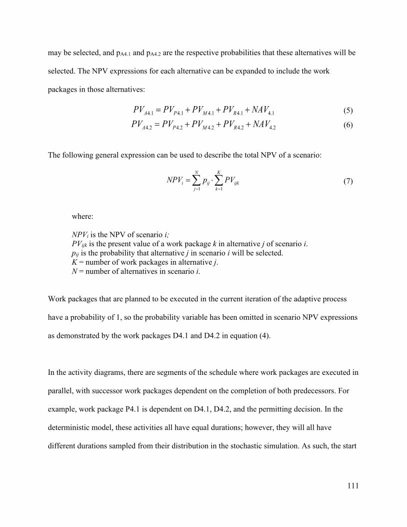
111

may be selected, and pA4.1 and pA4.2 are the respective probabilities that these alternatives will be

selected. The NPV expressions for each alternative can be expanded to include the work

packages in those alternatives:

4.1 4.1 4.1 4.1 4.1A P M RPV PV PV PV NAV= + + + (5)

4.2 4.2 4.2 4.2 4.2A P M RPV PV PV PV NAV= + + + (6)

The following general expression can be used to describe the total NPV of a scenario:

1 1

N K

i ij ijkj k

NPV p PV= =

= ⋅∑ ∑ (7)

where:

NPVi is the NPV of scenario i; PVijk is the present value of a work package k in alternative j of scenario i. pij is the probability that alternative j in scenario i will be selected. K = number of work packages in alternative j. N = number of alternatives in scenario i.

Work packages that are planned to be executed in the current iteration of the adaptive process

have a probability of 1, so the probability variable has been omitted in scenario NPV expressions

as demonstrated by the work packages D4.1 and D4.2 in equation (4).

In the activity diagrams, there are segments of the schedule where work packages are executed in

parallel, with successor work packages dependent on the completion of both predecessors. For

example, work package P4.1 is dependent on D4.1, D4.2, and the permitting decision. In the

deterministic model, these activities all have equal durations; however, they will all have

different durations sampled from their distribution in the stochastic simulation. As such, the start

112

of P4.1 is determined by the longest duration of the predecessor activities. The critical path

durations for these parallel work packages are defined in the model as:

Duration S4 Design & Permit T4.0 = max(TP, TD4.1, TD4.2) (8)

Duration A4.1 Construction/Development T4.1 = max(TC4.1, TM4.1) (9)

Duration A4.2 Construction/Development T4.2 = max(TC4.2, TM4.2) (10)

Using the continuous cash flow present value expressions in Appendix B.1, combined with the

work packages included in equations (4), (5), and (6) and the schedule segment critical path

durations shown in equations (8), (9), and (10), we can develop the present value formulas for

each work package. In this example, only uniform and trapezoidal gradient cash flow profiles are

used for the work packages. Negative signs before the cost variables indicate a cash flow out of

the project. For brevity, only the present value expressions for Scenario 4 have been included as

an example.

D4.1 4.1

4.14.1

4.10

DTrt D

DD

CPV e dtT

− −= ∫ (11)

D4.2 4.2

4.24.2

4.20

DTrt D

DD

CPV e dtT

− −= ∫ (12)

P4.1 4.1

4.0 4.14.1

4.10

PTrT rt C

CC

CPV e e dtT

− − −= ∫ (13)

113

M4.1 4.1

4.0 4.1 4.1( ) 4.14.1

4.10

M

M

Tr T T T rt M

MM

CPV e e dtT

− + − − −= ∫ (14)

R4.1 4.1

4.0 4.1( )4.1

0

( ( )(365)( ))RT

r T T rt F SR R S F R

R

P PPV e e F t P R V dtT

− + − −= − + + −∫ (15)

NAV4.1 4.0 4.1( )4.1

0

( ( )(365)( ) )LOMT

r T T rt LOMR LOM LOM LOM LOM

LOM

CPV e e F P R V dtT

− + −= − + − −∫ (16)

P4.2 4.2

4.0 4.24.2

4.20

PTrT rt C

CC

CPV e e dtT

− − −= ∫ (17)

M4.2 4.2

4.0 4.2 4.2( ) 4.24.2

4.20

M

M

Tr T T T rt M

MM

CPV e e dtT

− + − − −= ∫ (18)

R4.2 4.0 4.2( )4.2

0

( ( )(365)( ))RT

r T T rt F SR R S F R

R

P PPV e e F t P R V dtT

− + − −= − + + −∫ (19)

NAV4.2 4.0 4.2( )4.2

0

( ( )(365)( ) )LOMT

r T T rt LOMR LOM LOM LOM LOM

LOM

CPV e e F P R V dtT

− + −= − + − −∫ (20)

The critical path duration of the scenario can also be expressed through the duration variables of

the work packages in each alternative, summarized by the schedule segment critical path

durations included in equations (8), (9), and (10).

CPA4.1=T4.1+TR4.1 (21)

CPA4.2=T4.2+TR4.2 (22)

CPS4 = T4.0+pA4.1(CPA4.1)+pA4.2(CPA4.2) (23)

114

If the NPV of Scenario 4, NPVS4 and critical path duration of Scenario 4, CPS4 were evaluated

deterministically, this evaluation would use the weighted average of the NPV and critical paths

from the alternatives in that scenario. However, in the stochastic simulation, the alternative

probability variables will return either 0 or 1 to reflect that only one of the available alternatives

will be selected by the model in each simulation trial. The alternative uncertainty portion of the

stochastic simulation model is described further in section 5.4.1.

The structure and NPV expressions included in the model are specific to each risk management

situation in which the adaptive process and model are used. Developing the model requires

understanding the possible alternatives and work plans to implement these alternatives. While

each situation will follow the general structure outlined in this section and demonstrated through

the simple example, each situation will require a unique and customized system model with the

scenarios, alternatives, and work packages suitable to the risk management situation.

5.4 Stochastic Simulation Description

The stochastic simulation takes the system model introduced in section 5.3 and adds random

variable distributions for the work package variables and the alternative probabilities through a

Monte Carlo simulation. The stochastic simulation generates a probabilistic NPV result for each

scenario and calculates the value created by pursuing the adaptive approach. The simulation also

generates probabilistic results of other decision-making criteria of interest, such as critical path

duration of schedule segments and critical path duration of the overall schedule. The following

sections discuss the selection of distributions for the model variables, the probability model for

selecting alternatives, and describes the simulation process.

115

There are two areas of uncertainty that are included in the simulation. The first is the uncertainty

about which alternative will be required to resolve the risk. This aspect of model uncertainty is

discussed in section 5.4.1. The second is the uncertainty around work package variable estimates,

which are the inputs into the NPV calculations used in the model. This aspect of model

uncertainty is discussed in section 5.4.2.

5.4.1 Alternative Selection Uncertainty Model

The stochastic simulation includes an alternative uncertainty probability distribution that

simulates which of the risk resolution alternatives will be required to resolve the risk in each

simulation trial. This probability distribution is based on the uncertainty inherent in the risk

being managed and the method for modelling this uncertainty. This section includes a qualitative

description of how these alternative uncertainty models are created, while the specific

application of the uncertainty models for the case studies are discussed in Chapters 6 and 7.

The alternative uncertainty model generates the probabilities pij for each alternative in scenario i.

Returning to the example discussed in this chapter, the uncertainty being modelled is which

design alternative will be approved by the permitting authority. The uncertainty model used to

generate probabilities in this example could be based on either historical data of similar decisions

reached by the permitting authority or through a subjective assessment based on the expert

judgement on which alternative will be approved. As there are only two possible outcomes –

either Alternative 1 or Alternative 2 is approved – this could be represented with a Bernoulli

distribution that models the approval or rejection of Alternative 1. If Alternative 1 is selected,

then alternative 2 is rejected, and if Alternative 1 is rejected, then Alternative 2 is selected.

The probability mass function of this distribution would be:

116

1( , ) (1 ) k {0,1}k kf k p p p for−= − ∈ (24)

where p is the probability that Alternative 1 will be approved, and (1-p) is the probability that

Alternative 2 will be approved. In the simulation, the Bernoulli distribution will return the value

of k, which will be 1 when Alternative 1 is approved and 0 when Alternative 2 is approved. In

equation (4), pA4.1=k and pA4.2=(1-k) for each simulation trial.

The case studies included in this dissertation show two different types of alternative selection

uncertainty models. The alternative uncertainty model in the Chapter 6 case study is based on a

probability distribution of a deleterious element in an orebody. This probability distribution is

based on data obtained through geological drilling. As new drill samples are received, the

probability distribution is updated using Bayesian inference through successive iterations of the

adaptive process and updates to the system model. This shows how external data can be used in

the system model and stochastic simulation. The alternative uncertainty model in the Chapter 7

case study is similar to the example in this chapter. It is based on expert judgement, and as the

case study only requires a single iteration to identify the best alternative, it does not need to be

updated.

5.4.2 Work Package Variable Distributions

The work package cost and schedule variables are treated as continuous random variables in the

stochastic simulation and can take any probability distribution that the risk analyst or decision-

maker feels appropriate. It is suggested that the cost and schedule variables use a triangular

117

distribution for simplicity and improved acceptance in industry settings where there is less

familiarity with more specialized and uncommon probability distributions. Triangular

distributions are frequently recommended by project management professional associations

(AACEI, 2008b) and are attractive for many reasons. Triangular distributions are suitable when

the true underlying probability distribution is unknown or is difficult to determine, but an upper

and lower bound can be quickly estimated. Triangular distributions are suitable due to the one-

off nature of projects and the particularity of generating cost and schedule estimates for risk

response alternatives, often under time pressure and with limited information. Cost and schedule

estimates are conditioned on the degree of technical definition of the underlying work. If the cost

and schedule values are estimated through quantities and unit rates, it is straightforward to

estimate pessimistic and optimistic values for both quantities and rates to generate a maximum

and minimum value for total cost and duration. These values will be the endpoints of the

triangular distribution, with the deterministic estimate as the mode. Similarly, it is also

straightforward to use percent additions or reductions to the deterministic mode to generate

maximum and minimum. Many companies and organizations in the mining industry have

guidelines or benchmarks on percent values for range estimating. Other probability distributions

used in mining project development and recommended by professional associations include

uniform, beta, and PERT distributions (AACEI, 2008b). In the example described in this chapter

and the case studies presented in this dissertation, all the work package variables will use

triangular distributions.

Correlations between work package variables can be included in the model using Spearman rank

correlation coefficients. Spearman correlation is suitable for use in this application as it is a

distribution-free correlation method that allows different types of input variable distributions to

118

be correlated while preserving the integrity of those distributions and the random variables they

generate. This allows the flexibility to use different distribution types for model variables. In the

case studies explored in Chapters 6 and 7, correlations have been included between cost and

schedule variables within each work package for different work package types. Work packages

are assumed to be independent of each other.

5.4.3 Simulation Algorithm

The following is a summary of the process used in the stochastic simulation to generate the NPV

and critical path duration for the scenarios included in the model. The process describes the steps

required to generate values for all the model variables, calculate the NPV and critical path for

each alternative, use the alternative probability model to select an alternative, and output the

NPV and critical path of that alternative into the simulation results. While the process below

references equations and data tables for the example used in this chapter, the same process is

followed for all model applications.

1. For Scenario i=1 to N.

2. Sample values for all work package variables included in Table 5.1.

3. Calculate critical path of all schedule segments using equations (8), (9), and (10).

4. Calculate present value of all work packages using equations (11) to (20).

5. Calculate the present value of Alternative Aij using equations (5) and (6).

6. Generate pAij for all Alternatives Aij as described in section 5.4.1.

7. Calculate NPVi using equation (4).

8. Calculate CPi using equation (23).

9. Output NPVi and CPi results for the simulation trial.

119

10. Repeat steps 2-10 for specified number of simulation trials.

11. Repeat steps 2-11 for next i until i=N.

5.5 Interpreting Simulation Results and Outputs

Simulation results for both NPV and critical path duration are presented in two ways: cumulative

distribution functions (CDF) and box-whisker plots comparing each scenario. Box whisker plots

are used to show the results of all scenarios included in a stochastic simulation, as they clearly

summarise many different series of data. Cumulative distribution functions are used to show a

subset of the full results, comparing only the best-performing (highest ENPV) non-adaptive

scenario and the adaptive scenario. This is done to improve clarity in communicating the results

by only showing the two scenarios used to calculate the value of adaptivity.

The CDF for each scenario provides a more nuanced insight into the performance of scenarios

across the range of cumulative probabilities. The CDF shows which scenario best limits

downside risk in the lower cumulative probabilities or which has more potential upside in the

higher cumulative probabilities. This additional information is valuable given the risk

preferences of the decision-maker. If the decision-maker is risk-neutral - having linear risk-

preferences - they will select the scenario with the highest ENPV irrespective of the different risk

and uncertainty between scenarios. If decision-makers have non-linear risk preferences –risk-

averse or risk-seeking –they may choose scenarios that perform better at the lower or higher

cumulative probabilities. Two concepts that provide insight into the results while considering the

risk preferences of the decision-maker are stochastic dominance and Value-at-Risk (VaR)/Value

at Gain (VaG).

120

Stochastic dominance is a method for comparing two investment choices or scenarios to

determine if one scenario is superior to the others. Two measures of stochastic dominance are

first-order stochastic dominance (FOSD) and second-order stochastic dominance (SOSD.) Both

first and second order stochastic dominance tests identify the better-performing scenario relative

to the risk management objective and decision-maker preferences (Levy, 2016). Consider the

two scenarios shown in Figure 5.6.

Figure 5.6 Example CDF showing first order stochastic dominance.

First-order stochastic dominance is intuitive: on inspection, it is apparent that Scenario A

outperforms Scenario B for the objective function, NPV, as Scenario A has a higher NPV than

Scenario B across the entire range of cumulative probabilities. The first order stochastic

dominance test says that if Scenario A is FA(x) and Scenario B is FB(x), then Scenario A first-

order stochastically dominates Scenario B if:

( ) ( ) for all xA BF x F x≤ (25)

121

First-order stochastic dominance requires no limitations or assumptions on the risk preferences

of the decision-maker. This would apply to all risk-neutral (linear utility function), risk-averse

(concave utility function) or risk-seeking (convex utility function) decision-makers as it only

requires the utility function to be continuous and monotonically increasing.

A simple definition for second-order stochastic dominance is that a scenario achieves second

order stochastic dominance if it has less uncertainty and the range of possible outcomes is

smaller. Second-order stochastic dominance is also intuitive but requires more analysis than first-

order stochastic dominance. Consider the two scenarios shown in Figure 5.7.

Figure 5.7 Example CDF showing second order stochastic dominance.

Scenario A can be said to second-order stochastically dominate Scenario B if:

( ) ( ( ) ( )) 0 for all z

z

B AG z F x F x dx−∞

= − ≥∫ (26)

122

As shown in Figure 5.7, G(z) is greater than zero for all values of z=NPV, so Scenario A has

second-order stochastic dominance over Scenario B, so long as the ENPV for Scenario A is

greater than or equal to Scenario B, or EA(x) ≥ EB(x). Second-order stochastic dominance is

relevant as it indicates superiority between scenarios for a risk-averse decision-maker. Risk

aversion is not an overly restrictive or unrealistic assumption for a decision-maker in this

application, especially considering the significant financial investment required for mining

project development.

Value at Risk (VaR) and Value at Gain (VaG) are two metrics that can help decision-makers

identify which is the superior scenario given their risk preferences. VaR and VaG are similar in

concept to second-order stochastic dominance but require fewer conditions, do not make

assumptions about decision-makers' risk preferences, and do not constitute a test to determine

superiority. Instead, they simply provide more information for decision-makers with non-linear

risk preferences. Formally, VaR(α) and VaG(α) are the quantile functions of the variable x such

that there is α probability that x will fall below a certain level or α probability that x will exceed a

certain level. Figure 5.8 shows an example where ENPV is equal between Scenarios A and B,

but there are differences in VaR(α) and VaG(α).

123

Figure 5.8 Example CDF showing VaR(α) and VaG(α) where α=0.10

Unlike second-order stochastic dominance, VaR and VaG require no conditions on the ordering

of the expected payoff (ENPV) for each scenario. A risk-averse decision-maker may even prefer

a scenario with a lower expected return if it performs better at limiting downside risk and has

less uncertainty. Similarly, a risk-seeking decision-maker may prefer a scenario with lower

ENPV if it provides a much better potential for outsized gains. Although not shown in these

example figures, the asymmetry between how well a scenario limits downside risk without

sacrificing potential upside may be of particular importance to a decision-maker.

Stochastic dominance, value at risk, and value at gain provide important insight to the decision-

maker on the ordering and performance of available risk response scenarios. They provide an

intuitive lens to differentiate potential risk responses in light of risk preferences. Notwithstanding

the benefits of these tests and metrics, there are likely some alternate objectives or benefits that

are not formally included as objectives that could provide additional decision-making support.

When differences between ENPV are small, a decision-maker may choose to select the scenario

124

with the shorter schedule duration, one that uses a more familiar approach or technology, one

that is lower total cost, or one that is more robust to extreme variable ranges or outcomes.

Similarly, when differences in ENPV are small, the decision-maker may choose the scenario that

best protects against downside risk, even if it means selecting a lower ENPV. The utility function

that describes the preferences of the decision-maker would need to be understood to determine

which is the preferred scenario in this case.

The case studies in this dissertation assess which of the possible scenarios have the highest

ENPV and the ordering of scenarios as evaluated by first and second-order stochastic dominance.

For the purpose of this dissertation, the decision-maker is assumed to be risk-neutral and will

select the scenario with the highest ENPV. Notwithstanding, tests for stochastic dominance and

evaluation of VaR/VaG metrics have been provided in the following chapters to demonstrate

how different scenarios would be evaluated by decision-makers with non-linear risk preferences.

5.6 Conclusion

Knowing the performance of each risk resolution scenario relative to the objective function of

the project risk management process is necessary for informed decisions. Commonly used

project risk management methods do not provide adequate quantitative analysis in risk

management situations with high uncertainty, often leaving the decision-maker to select risk

management strategies based on superficial analysis or subjective assessments. The adaptive

system model and stochastic simulation provide quantitative support to the adaptive risk

management process and risk management decisions by comparing NPV - the objective function

of the system model - for all risk resolution scenarios and determining the value gained by

125

pursuing the adaptive scenario. The model also provides the decision-maker with additional

metrics of interest to help differentiate and order potential risk resolution scenarios.

While all applications of the adaptive system model and stochastic simulation have the same

general structure and format, each application is unique to the risk situation. Different

applications can have a different decision structure outlining the risk response scenarios,

differing numbers of technical alternative and work packages, and the uncertainty model

underlying the selection of alternatives and outcomes in the model can be different based on the

source of uncertainty and availability of data and information to model the uncertainty. For these

reasons, the description of the system model benefits from a detailed application and description

through case studies, which is the objective of Chapters 6 and 7.

126

Chapter 6: Exploring the Adaptive Process and Model

6.1 Case Study Introduction and Overview

To explore the adaptive process and system model described in Chapters 4 and 5, a structured

“toy problem” case study was developed. While the events, descriptions, and case study data

used in the analysis are synthetic, the case was inspired by a similar situation encountered by a

mining company during project development. The details and data used in the analysis were

generated to create a tractable case that allowed testing the full offering of the adaptive approach

while representing a detailed and realistic risk situation. Many of the processes and activities that

are ancillary to the objective of exploring the adaptive process, such as the detailed approach

taken to geological drilling and modelling, have been simplified to explore the adaptive case.

6.1.1 MineCo and the Arsenic Orebody Surprise

Mining Company Inc (MineCo) has recently purchased an old copper mine, Canyon Mine, that

had been placed on care and maintenance for several years. Canyon includes two existing

underground deposits, Alpha and Beta, and several undeveloped target deposits. As part of the

restart of operations, significant improvements and expansions are planned for the concentrator

plant processing facilities and the underground mine. The project team has completed a short

Feasibility Study and is nearing the start of project execution, which includes detailed

engineering, procurement, and construction. As MineCo is pursuing an aggressive project

development schedule to get the mine into operation as quickly as possible, the Feasibility Study

and detailed engineering completed to date used existing geological, metallurgical, and other

operations data from the previous mine operator.

127

In parallel with the Feasibility Study, the exploration team began a drilling campaign in one of

the high-potential exploration targets, called Gamma. Although the mine had a positive

economic evaluation with the existing reserves and resources from Alpha and Beta, the potential

for Gamma to have a large, high-grade orebody was an important consideration when MineCo

acquired Canyon. If drill results demonstrate that Gamma has higher copper grades than either

Alpha or Beta, MineCo will prioritize and fast-track Gamma development. MineCo intended to

complete underground development and rehabilitation at Alpha while exploring Gamma, then

developing Gamma and feeding the mill from both orebodies. Beta requires more extensive

development and rehabilitation, and under the current mine plan, it would not be mined for

several years.

Before the kickoff of project execution, the exploration team completes preliminary assays and

mineralogy test work on the drill samples from Gamma and confirms the presence of arsenic in

the form of arsenopyrite in the drill samples. The test work indicates high variability in arsenic

concentrations, with some of the samples showing negligible levels of arsenic, while others show

high levels. The arsenic levels were high enough that ore from Gamma could be economically

unviable with the processing methods designed in the Feasibility Study and under proposed

smelter agreement terms. Only ten samples were obtained in this initial drill program, so it is

unknown how much of the deposit is affected and what the actual arsenic concentrations are. The

exploration team cannot accurately assess the severity of this risk, and the engineering and

project team cannot determine the best course of action to manage or mitigate it. The overall

levels of arsenic may be low enough that no changes to the proposed restart are required, or

MineCo might be required to change either their mine plans or the process plant design to reduce

the arsenic levels in the concentrate.

128

6.1.2 Case Study Motivation and Methodology

The objective of the case study is to explore an application of the adaptive risk management

process in helping improve project risk analysis and risk management. This case is used to

explore the adaptive process as it exhibits the following:

• The risk of high levels of arsenic in Gamma has significant and lasting impacts on

MineCo and the operation of the mine. If sufficiently high, the deposit could be

economically unviable without treatment, which would reduce MineCo’s expected return

on investment.

• The strength of knowledge underlying the risk assessment is low. With only ten samples

in the initial drilling program, there is still considerable uncertainty about the

concentration of arsenic and how much of the orebody is affected.

• Knowledge can be improved through information gathering, such as additional drilling

campaigns, and experimentation, such as process design and metallurgical test work. This

information can be used to update the data used in the adaptive model.

• Several technically feasible alternatives are available. If the arsenic levels are low

enough, no additional treatment is required, but they must be managed either through ore

blending or an addition to the processing plant if they are sufficiently high.

• Resolving this risk requires considerable unanticipated work and could cause a

significant delay to the project baseline schedule. More drilling is required to improve the

knowledge about the orebody, and both the mining and processing alternatives require

additional study, design, and development/construction.

129

6.2 Framing the Adaptive Process

The following section describes how this risk could be managed using an adaptive process. The

descriptions below correspond to steps 1-5 of the adaptive process outlined in Chapter 4. Steps 6-

8 of the adaptive process are associated with developing the stochastic model and reviewing the

results; these steps are addressed in sections 6.3 and 6.4.

6.2.1 Risk Emergence: Drill Results show Arsenic in the Orebody

The signal that alerts the MineCo project team to the threat of arsenic in the orebody comes from

the assays and mineralogy tests on the initial drill samples from Gamma. The small number of

samples with high variability do not give the MineCo team high confidence that these samples

represent the actual concentration of arsenic in the orebody; however, these samples allow them

to identify potential alternatives to resolve the risk. The presence of deleterious elements in

copper orebodies is not uncommon, and it is known that arsenopyrite can occur in underground

copper deposits, so this risk was not unforeseeable. However, it was unexpected given that the

previous operator had not encountered significant amounts of arsenopyrite in existing

underground workings in Alpha or Beta deposits.

6.2.2 Characterizing the Risk

MineCo has an offtake agreement with a smelter for 100% of the concentrate produced at

Canyon. The smelter agreement stipulates penalty charges if the arsenic level in the concentrate

is above 0.3%, with progressively higher penalties up to a maximum allowable arsenic

concentration of 0.8%. MineCo completed a preliminary analysis using the initial Gamma drill

samples and the process modelling completed in the Feasibility Study to understand the effect of

arsenic in the orebody on arsenic levels in concentrate. The results of this analysis indicate a

130

wide range of possible outcomes under the mine plan and processing methods proposed in the

Feasibility Study. Arsenic levels may be low enough to draw no penalties, or they may be high

enough that either the smelter will not accept the concentrate, or the penalties will be

prohibitively high.

The epistemic uncertainty underlying this risk means the range of possible impacts is large due

to the low level of knowledge about the true arsenic concentration in the orebody. Fortunately,

the uncertainty can be reduced through additional drilling, assaying, and modelling. However,

even with a substantive drill program, there will still be lingering uncertainty that the modelled

probability distribution of arsenic accurately reflects the actual distribution of arsenic in the

orebody.

Initially, the strength of knowledge underlying this risk assessment is low. There is minimal

information available about the concentration of arsenic from the initial samples, and MineCo

has not spent a significant amount of time investigating possible design alternatives and their

effects on project cost and schedule. However, the actions required to improve knowledge and

confidence in both the risk assessment and the risk management plans are clear. Process and

mining studies can help MineCo better understand how arsenic in the orebody will translate to

arsenic in the concentrate and identify possible design alternatives to reduce the arsenic.

6.2.3 Defining the Risk Management Decision Space

MineCo has identified the risk management and decision objective in managing this risk is to

pursue the risk resolution scenario that maximizes NPV subject to capital cost constraints. The

total budget, including contingency for the project, is $422M, which includes the design and

131

construction of the processing plant and ancillary infrastructure, as well as mine development

and construction of mine services and infrastructure. The project contingency included in the

$422M is intended to account for the uncertainty and variability of costs and quantities in known

project scope and not for project scope changes and risks. MineCo has secured total project

financing of $475M, which includes an additional $53M project cost overrun facility to cover

any unexpected costs during project development outside the scope of the project contingency.

Any technical alternatives to resolve this risk must have less than $53M in incremental costs to

the project to be within the limitations of the project cost overrun facility. Impact on project

schedule is important to MineCo, although it is not considered a formal objective or a constraint.

If any of the risk resolution scenarios or design alternatives have negligible differences in NPV,

schedule duration may factor into decision making.

Additional analyses performed by MineCo show that implementing a resolution that reduces the

arsenic in concentrate to below 0.3% is preferable to a less costly resolution that still has a minor

refining penalty. NPV is more sensitive to the incremental operating costs that come from

penalties than increases in capital cost. As such, MineCo is only looking for alternatives that can

reduce the arsenic to below 0.3%.

6.2.4 Framing the Design Alternatives

Several possible design alternatives are available to MineCo to reduce the arsenic in concentrate

to below the penalty level. After a short period of study, MineCo has identified three possible

technical alternatives that could be implemented; the suitability and efficacy of each alternative

depends on the actual concentration of arsenic in the orebody:

132

1. Dilute the arsenic concentration in the ore by blending “dirty” ore from Gamma with

“clean” ore from Alpha and Beta before feeding the processing plant, resulting in lower

arsenic levels in the concentrate. The current mine plan only includes mining ore from

Alpha and Gamma, so this alternative includes additional development and rehabilitation

costs to bring Beta into production. The expected incremental cost of this alternative is

$37.5M, and the incremental schedule duration is three months.

2. Arsenic could be removed from the concentrate through a processing alternative, such as

partial roasting or a hydrometallurgical process designed to leach out the arsenic. This

alternative would require modifications and additions to the proposed process plant

design. The expected incremental cost of this alternative is $34.5M, and the incremental

schedule duration is six months.

3. MineCo could also reduce the levels of arsenic in the concentrate by blending the

concentrate produced at Canyon with an external concentrate source, either through

purchasing concentrate from a neighbouring mine or by acquiring a neighbouring mine

outright. The expected incremental cost of this alternative is significant, as an acquisition

of a property with sufficient production is expected to cost more than $400M. There is no

expected increase in schedule duration.

Each design alternative has a different strength of knowledge assessment that must be considered

in how the design alternatives are structured and evaluated. The ore blending alternative has a

medium strength of knowledge; it is not a technologically complex resolution and requires no

novel processes or equipment; it simply modifies and scales up the mine plan so that three

orebodies can be mined simultaneously instead of two. The ore processing option has a low

strength of knowledge. It requires additional facilities and technology not already considered in

133

the Feasibility Study design and requires additional operational expertise. The final alternative of

purchasing external concentrate or acquiring another operating mine has a low strength of

knowledge. It is not known whether a suitable mine can be found in the vicinity of Canyon and if

they have a suitable concentrate product specification.

The decision process, scenarios, and work packages to implement these potential design

alternatives are included in the stochastic model structure in section 6.3.

6.2.5 Aligning the Decisions Space and Design Alternatives

Multiple design alternatives for risk resolution are available, so these design alternatives must be

aligned with the decision space definition. The ore-blending and processing alternatives fall

within the capital cost constraints defined in the decision space, so these are acceptable

alternatives to include in the adaptive model. After a brief period of study, MineCo finds that

there are no nearby operating mines from which they can purchase concentrate to blend with

their concentrate, and the cost of acquiring a nearby operating mine is prohibitively high. This

alternative is rejected as it does not conform to the capital cost decision constraints. Preliminary

work plans are drafted for the remaining two alternatives with the work packages necessary to

implement the alternatives. These work packages are shown in the activity diagrams in Figure

6.1.

134

Figure 6.1 Activity diagrams for the baseline project plan and risk resolution alternatives

With potential design alternatives identified and aligned with the decision space, these

alternatives must be structured into different implementation scenarios and a decision structure

that will help model the value of pursuing an adaptive response to this risk.

6.3 Stochastic Model Structure

6.3.1 Planning the Adaptive Iterations

The MineCo team realizes that the information required to help identify the best risk resolution

alternative will come from three sources. Firstly, additional drilling will improve geological

models of the orebody resulting in a better arsenic concentration probability model. Secondly,

metallurgical tests, process design, and mine design will help validate the technical performance

of the various resolution alternatives. Thirdly, process and mine design studies will help improve

the cost and schedule estimates for the work packages required to implement these alternatives.

These three sources of information will help improve the strength of knowledge underlying the

risk assessment.

There is an inherent trade-off between the time spent gathering information, the quality and

quantity of information, and the time value of money spent acquiring that information. MineCo

1 2 3 4 5 6 7 8 9 10 11 12 13 14 15 16 17 18 19 20 21 22 23 24 25 26 27 28 29 30

Ore Blending Alternative

Process Change Alternative

Process Engineering Procurement Construction

Delay Start Mine Design Mine Development

Delay Start Engineering Procurement Construction

Mine Design Mine Development

Engineering Procurement Construction

Delay Start Mine Design Mine DevelopmentBaseline

Project Plan

135

decides to complete a six-month drill program, split into two stages of three months. They will

review the interim results at the end of each three months and incorporate the information into

the adaptive model and decision process. In the first three months, they expect to gather 40

additional drill samples for analysis, while in the second three months, they expect to gather an

additional 100 samples.

The staged drilling approach results in three iterations of the adaptive modelling and decision

process. The first iteration uses the initial ten drill samples to model the arsenic concentration.

The second iteration will use the 40 drill samples from the first three-month stage, and the third

iteration will use the 100 samples from the second three-month stage. Upon completing the six-

month drilling program, it is not expected that any new information gained through further

drilling will significantly improve the modelling and decision process. Figure 6.2 shows how the

adaptive approach is structured through the three iterations.

Figure 6.2 Structure of Iterative Adaptive Process

136

6.3.2 Scenarios and Design Alternatives

Based on the framing of the adaptive process described in the preceding section, the decision-

maker has three choices to manage this risk: halting project development until after the drilling

campaign is completed, immediately implementing one of the design alternatives while the

drilling campaign is ongoing, or managing the risk adaptively by pursuing multiple alternatives

in parallel with drilling. If the decision-maker chooses to pursue only a single alternative, they

must decide which alternative to pursue. The possible outcomes under this decision structure

form the basis of the scenarios and alternatives described in this section and are represented by

the decision tree shown in Figure 6.3. The alternatives represent the potential outcome of which

resolution will be implemented, while the scenarios represent the decision process to arrive at

those outcomes. For example, Alternative A3A.1 and A3B.1 result in the same risk resolution being

implemented but have different decision pathways to arrive at that outcome.

The scenarios and alternatives in the decision tree have been converted into activity diagrams,

which show the sequencing of all work packages. The activity diagrams show which work

packages will be executed in the next iteration of the adaptive process and the possible future

outcomes for each scenario. At the end of each adaptive iteration, the information gained from

the drilling campaign will be used to update the model. The remaining work for all scenarios and

alternatives will be replanned, and another iteration of the adaptive process will begin. At the

start of each adaptive iteration, the decision-maker faces the same choices described above and

must decide which scenario they want to pursue. This demonstrates flexibility even in the non-

adaptive scenarios: the decision-maker can change course and pursue a different scenario or

alternative based on the new drilling information received at the end of each adaptive iteration.

137

Figure 6.3 Decision tree for all case study scenarios

138

Scenario 1 (S1): Project Baseline Plan

Scenario 1 is the project baseline plan for the project. This scenario has been included in the

model and is described here to illustrate the baseline plan; however, the results have not been

included in section 6.4 since they do not influence the comparisons of the adaptive and non-

adaptive risk responses. Figure 6.4 shows the activity diagram for Scenario 1.

Figure 6.4 Activity diagram for Scenario 1

Scenario 2 (S2): Wait for Drilling

Scenario 2 is the risk response where project development is halted for the first three-month

adaptive iteration. In these three months, additional drilling is undertaken to improve knowledge

before deciding on an alternative. Figure 6.5 shows the activity diagram for Scenario 2.

Figure 6.5 Activity diagram for Scenario 2, Iteration 1

1 2 3 4 5 6 7 8 9 10 11 12 13 14 15 16 17 18 19 20 21 22 23 24 25 26 27 28 29 30 31 32 33 34Engineering Procurement Construction


1 2 3 4 5 6 7 8 9 10 11 12 13 14 15 16 17 18 19 20 21 22 23 24 25 26 27 28 29 30 31 32 33 34

A2.1

pA2.1 = 0.166

A2.2

pA2.2 = 0.382

A2.3

pA2.3 = 0.452

Mine Development

Process Engineering Procurement Construction

Delay Start Mine Design

Mine Design

Drilling



Mine Development

Mine Development


139

Scenario 3A (S3A): Continue with Baseline Plan (No Change)

Scenario 3A is the risk response plan where the decision is made to proceed with Alternative 1

and continue with the project baseline plan while conducting the three-month drilling campaign.

The only work package in Scenario 3A to be completed in parallel with the drilling is the

engineering work package. Once drilling is complete, the decision on which alternative to pursue

– either continuing with Alternative 1 or switching to either of the other two alternatives – will

be made. Figure 6.6 shows the activity diagram for Scenario 3A.

Figure 6.6 Activity diagram for Scenario 3A, Iteration 1

Scenario 3B (S3B): Pursue Ore Blending

Scenario 3B is the risk response plan that proceeds with Alternative 2 to develop Beta deposit so

ore-blending can reduce the arsenic concentration in the concentrate. The only work package in

Scenario 3B to be completed in parallel with the drilling is the mine design work package for

Beta deposit mine design. Figure 6.7 shows the activity diagram for this Scenario 3B.

1 2 3 4 5 6 7 8 9 10 11 12 13 14 15 16 17 18 19 20 21 22 23 24 25 26 27 28 29 30 31 32 33 34

A3A.1

p3A.1 = 0.166

A3A.2

p3B.2 = 0.382

A3A.3

p3C.3 = 0.452

Procurement Construction




Process Engineering

Construction


Delay Start Engineering

DrillingEngineering

Engineering Procurement

140

Figure 6.7 Activity diagram for Scenario 3B, Iteration 1

Scenario 3C (S3C): Pursue Process Changes

Scenario 3C is the risk response plan that proceeds with Alternative 3 to design additional plant

facilities for a hydrometallurgical or pyrometallurgical process. The only work package in

Scenario 3C to be completed in parallel with the drilling is the process design work package.

Figure 6.8 shows the activity diagram for this Scenario 3C.

Figure 6.8 Activity diagram for Scenario 3C, Iteration 1

Scenario 4 (S4): Adaptive Response

Scenario 4 is the adaptive risk response plan where the next sequential work packages for all

alternatives are pursued. Similar to the other scenarios, the work will be completed in parallel

with the drilling campaign, but at the end of the drilling, if enough information has been gathered

1 2 3 4 5 6 7 8 9 10 11 12 13 14 15 16 17 18 19 20 21 22 23 24 25 26 27 28 29 30 31 32 33 34

A3B.1

p3B1 = 0.166

A3B.2

p3B.2 = 0.382 Mine Design

A3B.3

p3B.3 = 0.452


Delay Start Mine Development


Mine Development

Process Engineering

Mine Design



Drilling

1 2 3 4 5 6 7 8 9 10 11 12 13 14 15 16 17 18 19 20 21 22 23 24 25 26 27 28 29 30 31 32 33 34

A3C.1

p3C.1 = 0.166

A3C.2

p3C.2 = 0.382

A3C.3

p3C.3 = 0.452







DrillingProcess

141

to identify the best alternative, this alternative will be continued while the others will be

abandoned. The work packages to be completed in parallel with the drilling include engineering,

mine design, and process design. Figure 6.9 shows the activity diagram for this Scenario 3C.


The activity diagrams for all five scenarios in three iterations of the adaptive process are not

shown here but are included in Appendix C.1. However, to illustrate and further describe the

iterative adaptive process, the activity diagrams for Iterations 2 and 3 for Scenario 4 are shown in

Figure 6.10 and Figure 6.11. These show how the adaptive process continues by adding the

subsequent work packages for each remaining alternative through successive iterations. The

dotted line in both figures shows the time the iterations start; all work packages to the right of the

line are in the current or future iterations, while all work packages to the left have been

completed in previous iterations.

1 2 3 4 5 6 7 8 9 10 11 12 13 14 15 16 17 18 19 20 21 22 23 24 25 26 27 28 29 30 31 32 33 34

A4.1

p4.1 = 0.166

A4.2 Engineering

p4.2 = 0.382

A4.3

p4.3 = 0.452 Delay Start Mine Development

Construction





Delay Start Procurement

ProcessMine DesignEngineering

Engineering

Drilling

142



6.3.3 Work Packages, Model Variables, and Distributions

The different scenarios included in the model have similar or identical work packages, as shown

in the figures in the preceding section and Appendix C.1. Although the work package scope and

estimated values may be identical or similar, the work package sequencing differs between

scenarios. Table 6.1 shows the work packages and model variables for each work package and

1 2 3 4 5 6 7 8 9 10 11 12 13 14 15 16 17 18 19 20 21 22 23 24 25 26 27 28 29 30 31 32

A4.1

pA4.1 = 0.028

A4.2

pA4.2 = 0.477

A4.3

pA4.3 = 0.495



Engineering Engineering

Procurement


Delay Start Procurement Construction

Mine Development

Drilling DrillingProcess

Mine Design Mine Design

Construction

1 2 3 4 5 6 7 8 9 10 11 12 13 14 15 16 17 18 19 20 21 22 23 24 25 26 27 28 29 30 31 32

A4.1

pA4.1 = 0.000

A4.2

pA4.2 = 0.234

A4.3

pA4.3 = 0.766

Mine Development - Deposit 1+2 (D1 + D2)

Construction

Mine Development - Deposit 1 (D1) Early Finish

Procure (Main Plant)Procure (New Process)

Mine Dev (D1 + D2)

Construction

Mine Development - Heading 1

Delay Start Construction


Mine Design Mine DesignEngineering Engineering

143

includes the cash flow profile and variable distribution shapes. The model variable values and

ranges for all scenarios in Iteration 1 are shown in Appendix C.2 as an example of the data that

was used in the model simulation.

Table 6.1 Work packages, cash flow profile shapes, and model variable distributions.

Work Package Variable Symbol Units Cash flow Profile

Variable Distribution

Construction (CC) Cost C.CC $ Uniform Triangular Duration T.CC Years Triangular

Drill and Assay (DA) Cost C.CC $ Uniform Triangular Duration T.CC Years Triangular

Engineering (EN) Cost C.CC $ Uniform Triangular Duration T.CC Years Triangular

Mine Design (MD) Cost C.CC $ Uniform Triangular Duration T.CC Years Triangular

Mine Development (DV)

Cost C.CC $ Uniform Triangular Duration T.CC Years Triangular

Process Design (PD) Cost C.CC $ Uniform Triangular Duration T.CC Years Triangular

Procurement (PU) Cost C.CC $ Uniform Triangular Duration T.CC Years Triangular

Production Ramp-up (PR)

Throughput P.PR Tonne/Day Gradient Triangular Duration T.PR Years Triangular Fixed OPEX F.PR $/Year Triangular Variable OPEX V.PR $/Tonne Triangular

The descriptions of the work packages identified in Table 6.1 are as follows:

• Construction (CC): Includes all activities required to construct and commission the

processing plant. For the process change alternative, this includes the additional

processing facilities.

• Drill and Assay (DA): Includes all activities to drill, log core, assay, update appropriate

geological models, and update results of arsenic concentration in the new drill samples.

144

• Engineering (EN): Includes all activities to design and specify equipment and complete

detailed construction drawings for the process plant and ancillary facilities.

• Mine Design (MD): Includes all activities required to develop the mine plan, mine

schedule, and specifying mine equipment and ancillary equipment and services.

Depending on the scenario and alternative, this work package could include mine design

for only Alpha and Gamma, or Alpha, Beta, and Gamma.

• Mine Development (DV): Includes all activities required for mine development to drive

ramps, level access, and any other underground workings to gain access to the orebody.

• Process Design (WP): Includes all activities required to do the test work, preliminary

process flow diagrams, and prove the technical feasibility of the processing equipment

required for the Process Change alternative.

• Procurement (PU): Includes the tender, award, fabrication, and delivery of all

equipment and materials required for the processing plant and ancillary facilities.

• Production Ramp-up (PR): Includes all activities required to ramp the plant up to full

production following construction and commissioning.

Global model variables, such as commodity prices and production variables, apply to all work

packages. The Life-of-Mine variables used to calculate the NAV in the model use deterministic

values. Using deterministic values for NAV variables allowed the effects of pursuing either an

adaptive or non-adaptive response to the risk to be isolated and seen much more clearly. The

adaptive process focuses on maximizing value in the construction stage through an adaptive

approach to risk management; only through isolating the contribution of the adaptive approach

145

was it possible to see how each scenario performed across the range of cumulative probabilities

resulting from the simulation.

During successive iterations of the adaptive process, new information and knowledge gained in

the preceding iterations is used to update both the base estimate (mode) values for the variables

listed in Table 6.1 and the ranges of minimum and maximum values used in the triangular

distributions. This information gains achieved through the information gathering work packages,

such as drilling and assaying, process design, and mine design, reduce the epistemic uncertainty

underlying the assessment of the base estimate and ranges. This reduction in uncertainty can be

expressed through an improved strength of knowledge assessment, and as knowledge improves,

the distribution ranges become smaller. For this case study, the strength of knowledge

assessment follows a simple ordinal scale Low, Medium, and High classifications. Table 6.2

shows the ranges for the triangular distribution minimum and maximum values, categorized by

cost type.

Work packages have been grouped into similar cost types reflecting the nature of the work, as

these are assumed to have similar ranges. These ranges were estimated based on industry

guidelines and recommended practices and reflect the technical definition available when the

estimates were made. The low and high percentage ranges are relative to the base estimate

(mode) value used in the distribution.

146

Table 6.2 Strength of Knowledge (SoK) assessments and variable uncertainty ranges

Type Variable Low SoK Medium SoK High SoK Fabrication / Construction / Field Work

Duration -15.0% 35.0% -10.0% 25.0% -5.0% 15.0% Cost -20.0% 30.0% -12.5% 20.0% -5.0% 10.0%

Engineering / Design Duration -25.0% 35.0% -20.0% 30.0% -15.0% 25.0% Cost -20.0% 25.0% -15.0% 20.0% -10.0% 15.0%

6.3.4 Arsenic Concentration Uncertainty Model

The stochastic model developed for this case study follows the general model structure described

in Chapter 5. All the scenarios included in the model have three alternatives that represent the

possible alternative outcomes, as shown by the decision tree in Figure 6.3. The arsenic

concentration probability distribution governs the selection of alternatives in each simulation

trial: the technical alternative required is based on the simulated arsenic concentration. The

model simulates the NPV for all the alternatives based on the work packages and variables

described in section 6.3.3. The simulated NPV for any scenario Si is selected from the NPV of

each alternative in that scenario, where x is the simulated arsenic concentration:

.1

.2

.3

for x 0.065% No changes required.

for 0.065 < x 0.08% Ore blending required.

for x >0.08% Process changes required.

Ai

Si Ai

Ai

NPVNPV NPV

NPV

≤

≤

=

(27)

As described in Chapter 5, the system model is updated in successive iterations of the adaptive

process based on new information. The initial arsenic concentration probability distribution is

based on the first set of ten samples drilled by the geology and exploration team. The arsenic

concentration probability distribution is then updated through each iteration of the adaptive

147

process using Bayesian inference. The initial arsenic probability distribution is assumed to be

normal and has a sample mean �̅�𝑥=0.07833% and a standard deviation σ=0.04354%. Using these

initial sample parameters and assuming a diffuse prior distribution, the posterior distribution

used for the first adaptive process iteration is given by:

( ) ( ) ( , )f kL N xnµσµ µ′′ = = (28)

A diffuse prior was used in the first iteration, as it is a conservative approach to modelling the

arsenic concentrations that minimizes the potential impact of using an “incorrect” prior. If, for

example, the prior distribution had assumed very low arsenic concentrations, this would affect

the posterior distribution used in the first iteration of the model and would likely have affected

the results and decision recommendation generated by the model.

Evaluating equation (28) with the sample mean and standard deviation from the initial 10

samples results in the normal posterior distribution N(0.07833,0.01377) used for the first

iteration of the adaptive process. The probability density function and the cumulative distribution

function for this distribution are shown in Figure 6.12 and Figure 6.13, respectively, with

annotations showing the values for which each of the technical alternatives will be selected

during the simulation.

148

Figure 6.12 Posterior PDF of arsenic concentration, Iteration 1.

Figure 6.13 Posterior CDF of arsenic concentration, Iteration 1.

In the second and third iterations of the adaptive process, the probability distribution of arsenic

concentration is updated through Bayesian inferences using the new sample data obtained from

the drilling campaigns. In the second and third iterations, the posterior distribution from the

preceding iteration becomes the new prior distribution. Since both the prior and likelihood

distributions represent the same underlying random variable and are both normally distributed,

149

the prior and posterior distributions are conjugate pairs and the posterior parameters can be

obtained analytically using the following relationships:

2 2

2 2

( )( )

n xn

µ µµ

µ

µ σ σµ

σ σ′ ′+

′′ =′+

(29)

2 2

2 2

( ) ( )( ) ( )

nn

µµ

µ

σ σσ

σ σ′

′′ =′ +

(30)

Where µµ′′ and µσ ′′ are the mean and standard deviation of the posterior distribution, µµ′ and µσ ′

are the mean and standard deviation of the prior distribution, and x and σ are the sample mean

and standard deviation of the likelihood, while n is the likelihood sample size. The results of this

updating have been included in Table 6.3. The inclusion of these results in the model and the

implications for the model results are discussed in section 6.4.

Table 6.3 Prior, likelihood, and posterior distributions of arsenic concentration, Iterations 1-3

Samples (n) Prior Likelihood

Iteration 1 Initial drilling samples

10

Prior Diffuse Prior

Likelihood N(0.07833, 0.01377)

Posterior N(0.07833, 0.01377)

Iteration 2 Samples from iteration 1 drill/assay.

40

Prior N(0.07833, 0.01377)

Likelihood N(0.08064, 0.00949)

Posterior N(0.07989, 0.00781)

Iteration 3 Samples from iteration 2 drill/assay.

100

Prior N(0.07989, 0.00781)

Likelihood N(0.08392,0.00461)

Posterior N(0.082879,0.00397)

150

6.4 Simulation Results

The results of all three iterations of the adaptive process are presented, which include a summary

of both the NPV and critical path duration results. The results are evaluated primarily by ENPV,

with additional comments related to stochastic dominance and value at risk, as introduced in

Chapter 5, to compare performance across the full range of cumulative probabilities. Although

not considered as an objective function, the critical path results are presented as they are likely a

metric of interest for decision-makers.

6.4.1 First Adaptive Iteration

The first adaptive iteration includes preparing and running the stochastic model simulation based

on the scenarios, alternatives, and work packages identified in section 6.3, using the initial 10

drill samples to develop the arsenic concentration probability distribution. For the first iteration,

the arsenic concentration PDF and CDF are shown in the previous section in Figure 6.12 and

Figure 6.13, respectively. As this is the first iteration, and a diffuse prior is used, only a posterior

distribution is available. Subsequent updates of the arsenic concentration probability distribution

will include prior, likelihood, and posterior distributions.

The adaptive model was populated with the variable estimates for the first iteration, and the

simulation was run to determine the value for each scenario. Table 6.4 summarizes the results

from the first iteration modelling showing that the adaptive response has an ENPV of $436.8M

compared to the best performing non-adaptive response, Scenario 3A – Continue with Base Plan,

which has an ENPV of $431.9M. Pursuing the adaptive response scenario has positive value in

151

the first iteration of the adaptive process. Based on these results, MineCo can execute the works

packages planned for the three-month duration of the first iteration.

Table 6.4 ENPV for all modelled scenarios, Iteration 1

Description ENPV Scenario 2 Wait for Drilling Results $428.7M Scenario 3A Continue with Base Plan* $431.9M Scenario 3B Implement Ore Blending Alternative $430.1M Scenario 3B Implement Process Change Alternative $430.5M Scenario 4 Adaptive Response $436.8M Expected Value of Adaptivity $4.9M *denotes the highest ENPV non-adaptive alternative

While the ENPV results show the expected value of adaptivity is $4.9M, the box whisker plot

and cumulative distribution function in Figure 6.14 and Figure 6.15 show a complete comparison

of the adaptive and non-adaptive response scenarios. The cumulative distribution function shows

that the adaptive response outperforms the highest-value non-adaptive response through most of

the cumulative distribution function; it underperforms the non-adaptive scenario at

approximately the P85 value and above. This is because the non-adaptive scenario has a higher

NPV for the model simulations where Alternative 1 “No Change Required” is selected. Since

this alternative requires only continuing with the base plan, the scenario where executing only

the work packages included in the base plan outperforms the adaptive scenario.

152

Figure 6.14 NPV box-whisker plot, Iteration 1

Figure 6.15 NPV cumulative distribution function, Iteration 1

Comparing the cumulative distribution functions shows that the adaptive response fails the first-

order stochastic dominance test over the non-adaptive response but passes the second order

stochastic dominance test. This shows that a risk-averse decision-maker will prefer the adaptive

response over the non-adaptive response. Table 6.5 shows the Value at Risk and Value at Gain

values for the stochastic model results. These results show the asymmetry between the adaptive

153

and non-adaptive responses at the extreme ends of the cumulative distribution function; the

adaptive response protects much better against downside loss than it limits upside gain.

Table 6.5 NPV Value at Risk and Gain (VaR/VaG) for (α=.05), Iteration 1

Description NPV VaR(0.05) Scenario 3A Continue with Baseline Plan (No Change) $353.1M VaR(0.05) Scenario 4 Adaptive Response $358.2M Adaptive Response VaR(0.05) $5.1M VaR(0.95) Scenario 3A Continue with Baseline Plan (No Change) $506.6M VaR(0.95) Scenario 4 Adaptive Response $506.1M Adaptive Response VaG(0.95) -$0.5M

When comparing the adaptive response and looking at the value gained through pursuing an

adaptive approach, it initially appears that the value gain from adaptivity is minimal, only a 1%

gain over the non-adaptive responses. The question then arises of whether pursuing an adaptive

approach is worth the extra effort and resources given the small increase in value. However, the

cost of acquiring flexibility in risk management through the adaptive response is already built

into the analysis. If the extra effort and resources can be expressed solely in financial terms, they

have been accounted for, and the adaptive approach still creates incremental value. In addition,

as it outperforms the non-adaptive response specifically at the lower cumulative probabilities, it

is an effective tool to protect against loss.

In addition to the increase in value, the adaptive response has a shorter expected critical path

duration to complete the project and achieve full production. Construction duration has been

considered in the NPV analysis through discounting and the time-cost of money. Although

schedule performance is not included as an objective, it may be meaningful to decision-makers,

especially where increases in ENPV are small. As shown in the critical path simulation results in

154

Table 6.6, the adaptive response has a shorter critical path duration, with an expected schedule

acceleration of 0.20 years (2.4 months) over the non-adaptive scenario. This is intuitive, as the

adaptive response creates value by shortening the time to full mine production; however, the

results can be assessed together. The choice then is between two ways to manage the risk: the

adaptive response resolves the risk while increasing value and reducing the duration to full

production, whereas the non-adaptive response takes longer and is lower value.

The critical path duration results are shown in Table 6.6 and Figure 6.16. The results table shows

that the adaptive response has an expected critical path duration of 2.89 years, 0.20 years less

than the best performing non-adaptive response. The descending cumulative distribution function

shows that the adaptive response outperforms the non-adaptive response for most of the

cumulative probabilities. A descending cumulative distribution function was used to show the

results of the critical path duration simulation as a descending curve is suitable when the

measurement of interest – in this case, the critical path duration – is one where a smaller value is

favourable. Similar to the results of the NPV modelling, the adaptive response performs much

better than the non-adaptive response at the lower end of the cumulative distribution function.

Table 6.6 Expected critical path durations for all scenarios, Iteration 1

Description Duration (TCP) Scenario 2 Wait for Drilling Results 3.24 years Scenario 3A Continue with Base Plan* 3.09 years Scenario 3B Implement Ore Blending Alternative 3.18 years Scenario 3B Implement Process Change Alternative 3.16 years Scenario 4 Adaptive Response 2.89 years Expected schedule reduction of Adaptivity 0.20 years *denotes the shortest duration non-adaptive alternative

155

Figure 6.16 Critical path cumulative distribution function (descending), Iteration 1

Based on the first iteration of the adaptive model, the MineCo team implements the work

packages included in the adaptive scenario work plan for the first iteration. This includes a

planned three-month drilling campaign to obtain 40 additional samples, advancing the base

design engineering, completing the process design and metallurgical test work, and advancing

the mine designs for Alpha, Beta, and Gamma deposits. Once these work packages are complete,

MineCo can compile the new information received and proceed with the second iteration of the

adaptive process.

6.4.2 Second Adaptive Iteration

The information gained during the first adaptive iteration was input into the model and used to

simulate the value of pursuing an adaptive response for another three months while the second

three-month stage of drilling was completed. The observations, tests, and design work completed

in the first iteration resulted in the following improvements to information and knowledge:

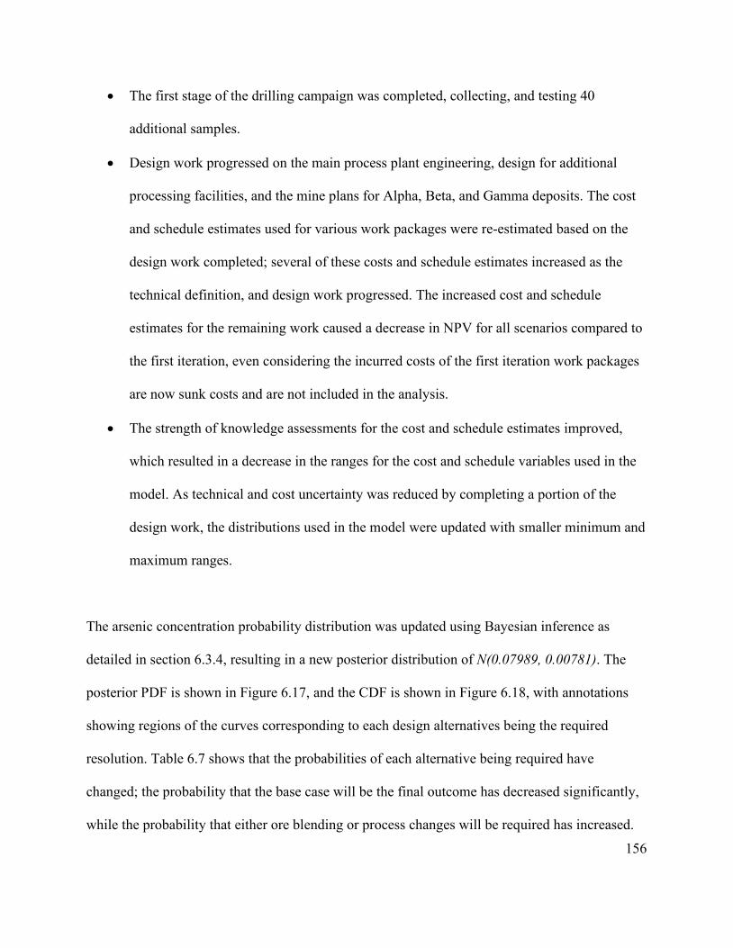
156

• The first stage of the drilling campaign was completed, collecting, and testing 40

additional samples.

• Design work progressed on the main process plant engineering, design for additional

processing facilities, and the mine plans for Alpha, Beta, and Gamma deposits. The cost

and schedule estimates used for various work packages were re-estimated based on the

design work completed; several of these costs and schedule estimates increased as the

technical definition, and design work progressed. The increased cost and schedule

estimates for the remaining work caused a decrease in NPV for all scenarios compared to

the first iteration, even considering the incurred costs of the first iteration work packages

are now sunk costs and are not included in the analysis.

• The strength of knowledge assessments for the cost and schedule estimates improved,

which resulted in a decrease in the ranges for the cost and schedule variables used in the

model. As technical and cost uncertainty was reduced by completing a portion of the

design work, the distributions used in the model were updated with smaller minimum and

maximum ranges.

The arsenic concentration probability distribution was updated using Bayesian inference as

detailed in section 6.3.4, resulting in a new posterior distribution of N(0.07989, 0.00781). The

posterior PDF is shown in Figure 6.17, and the CDF is shown in Figure 6.18, with annotations

showing regions of the curves corresponding to each design alternatives being the required

resolution. Table 6.7 shows that the probabilities of each alternative being required have

changed; the probability that the base case will be the final outcome has decreased significantly,

while the probability that either ore blending or process changes will be required has increased.

157

Figure 6.17 Probability density function of arsenic concentration in orebody, Iteration 2.

Figure 6.18 Cumulative distribution function of arsenic concentration in orebody, Iteration 2.

158

Table 6.7 Updated probabilities for alternative selection, Iteration 2.

Alternative Description Alternative Probabilities

Iteration 1 Iteration 2 Alternative 1 (Ax.1) No change required. 0.166 0.028 Alternative 2 (Ax.2) Ore blending required. 0.382 0.477 Alternative 3 (Ax.3) Process changes required. 0.452 0.495

The results of the second iteration model show that there is still a positive ENPV in pursuing the

adaptive scenario over the non-adaptive scenarios. Table 6.4 shows the adaptive scenario has an

ENPV of $399.9M, compared to the best performing non-adaptive response, “Scenario 3C –

Implement Process Change Alternative”, which has an ENPV of $397.6M. The best performing

of the non-adaptive responses has changed in the second iteration, with Scenario 3A no longer

being the highest NPV of the non-adaptive responses. This change is primarily due to the updates

in the arsenic probability distribution and the decrease in the probability that no change will be

required. However, the respective NPVs for each of the non-adaptive single alternative scenarios

3A, 3B, and 3C are still very clustered, as the additional cost of executing work packages in the

second iteration for Scenarios 3B and 3C is nearly equal to the value gained through schedule

acceleration. All the work packages included in Scenario 3A are included in the other scenarios,

so there is no penalty for completing unnecessary work in alternative 3A. Although the

probability of no changes being required has decreased considerably, there is still significant

uncertainty about which of the ore blending and process changes alternatives will be required.

The second iteration shows a decrease in the value of adaptivity compared to the first iteration.

This decrease is expected and intuitive. Since the adaptive scenario was pursued in the first

iteration, the designs for all the alternatives were advanced; in the second iteration, all scenarios

159

benefit from the work performed in the first iteration adaptive scenario. The benefit of this work

is reflected in the remaining work packages and activity diagrams for the non-adaptive scenarios.

The value of flexibility will tend to decrease as uncertainty decreases; as such, the value of

adaptivity decreases as new information gained reduces uncertainty in the system.

Table 6.8 ENPV for all modelled scenarios; Iteration 2

Description ENPV Scenario 2 Wait for Drilling Results $395.9M Scenario 3A Continue with Base Plan $397.4M Scenario 3B Implement Ore Blending Alternative $396.7M Scenario 3B Implement Process Change Alternative* $397.6M Scenario 4 Adaptive Response $399.9M Expected Value of Adaptivity $2.2M *denotes the highest ENPV non-adaptive alternative

While ENPV points to an expected value of adaptivity of $2.2M, the box whisker plot and CDF

in Figure 6.19 and Figure 6.20 provide more details on the range of possible outcomes and

distribution of results. Unlike the first iteration, the best performing non-adaptive response now

performs better at the lower cumulative probabilities than the adaptive response. Similar to the

expected NPV, this change is partly due to the updates in the arsenic probability model and the

NPV calculations for the alternatives within each scenario. Alternative 1 (Ax.1) has the highest

NPV amongst the three alternatives. In the first iteration, its inclusion in the model increased the

ENPV and the NPV results in the higher cumulative probabilities. As the probability of

Alternative 1 decreased in the second iteration, its contribution to the overall NPV has also

decreased. Since the Process Change alternative, Alternative 3 (Ax.3), has the lowest NPV

amongst the three alternatives, it is expressed in the lower cumulative probabilities. Pursuing

160

Scenario 3C results in the fastest implementation of Alternative 3, so it outperforms the adaptive

response in the lower region of the CDF.


Figure 6.20 NPV cumulative distribution, Iteration 2

The second iteration differs from the first as the adaptive scenario no longer has second order

stochastic dominance over the non-adaptive scenario. This is due to the slight overperformance

161

of the non-adaptive scenario at the lower cumulative probabilities. The VaR and VaG metrics are

summarized in Table 6.9.

Table 6.9 NPV Value at Risk and Gain (VaR/VaG) for (α=.05), Iteration 2

Description NPV VaR(0.05) Scenario 3C Implement Process Change Alternative $329.1M VaR(0.05) Scenario 4 Adaptive Response $326.9M Adaptive Response VaR(0.05) -$2.2M VaR(0.95) Scenario 3C Implement Process Change Alternative $462.8M VaR(0.95) Scenario 4 Adaptive Response $469.1M Adaptive Response VaG(0.95) $6.3M

Notwithstanding the changes in stochastic dominance and VaR/VaG, pursuing the adaptive

response is still the preferred decision with a higher ENPV than the non-adaptive responses. In

this iteration, pursuing the adaptive response enables the opportunity to improve project value if

the future arsenic drilling results show lower concentrations in the orebody. In addition to the

NPV results, the critical path duration of the adaptive response outperforms the non-adaptive

responses, shown in Table 6.10. When the value of adaptivity is positive but small, and the

adaptive scenario does not have first or second order stochastic dominance, a decision-maker

may wish to include schedule performance in their decision-making process. This hierarchy of

decision considerations makes sense in a project risk management setting: where two risk

resolution scenarios have similar ENPVs, neither scenario has first or second order stochastic

dominance, then a decision-maker may look to another differentiating factor of interest, such as

schedule or cost. When presented with equivalent scenarios on the metrics listed previously, the

one that achieves resolution faster will likely be preferred. Figure 6.21 shows the descending

CDF of the critical path duration.

162


Description Duration (TCP) Scenario 2 Wait for Drilling Results 3.16 years Scenario 3A Continue with Base Plan 3.05 years Scenario 3B Implement Ore Blending Alternative 3.10 years Scenario 3B Implement Process Change Alternative* 3.05 years Scenario 4 Adaptive Response 2.93 years Expected schedule reduction of Adaptivity 0.12 years *denotes the shortest duration non-adaptive alternative


Based on the analysis completed and the positive value of pursuing the adaptive approach

predicted in the second iteration of the adaptive model, the MineCo team implements the work

packages included in the second iteration adaptive scenario work plan. This includes the second

three-month drilling campaign to obtain 100 additional samples, advancing the remaining

engineering work for the main plant and the processing additions, and completing the mine plans

for Alpha, Beta, and Gamma deposits.

163

6.4.3 Third Adaptive Iteration

The improvement to information and knowledge gained in the second iterations and input into

the model for the third iteration includes the following:

• The second and final stage of the drilling campaign was completed, with 100 new

samples collected, resulting in 150 total samples.

• Work was completed on the main process plant engineering and the arsenic processing

circuit designs, and the mine plans for Alpha, Beta, and Gamma deposits.

• The cost and schedule estimates used for the procurement, construction, and mine

development work packages were updated based on the final detailed design. As the cost

and schedule estimates are based on construction-level drawings, the uncertainty around

quantities and unit costs decreased, resulting in improved strength of knowledge and

smaller ranges for the model variables.

The arsenic concentration probability distribution was updated with the new information from

the final 100 drill samples, again using Bayesian inference as detailed in section 6.3.4. The new

posterior distribution of the arsenic concentration is N(0.082879,0.00397) with a PDF in Figure

6.22 and an annotated CDF in Figure 6.23. Table 6.11 shows the updated probabilities for each

alternative, with significant changes from the second iteration. The probability that ore

processing will be the required alternative to resolve the risk has increased substantially.

164

Figure 6.22 PDF of arsenic concentration in orebody, Iteration 3

Figure 6.23 CDF of arsenic concentration in orebody, Iteration 3

Table 6.11 Updated probabilities for alternative selection, Iteration 3

Alternative Description Alternative Probabilities

Iteration 1 Iteration 2 Iteration 3 Alternative 1 (Ax.1) No change required. 0.166 0.028 0.000 Alternative 2 (Ax.2) Ore blending required. 0.382 0.477 0.234 Alternative 3 (Ax.3) Process changes required. 0.452 0.495 0.766

165

In the third adaptive iteration, the adaptive scenario no longer has the highest ENPV. Table 6.12

shows the ENPV values for all scenarios; the adaptive scenario ENPV of $379.7M is $8.5M less

than the best-performing non-adaptive alternative with an ENPV of $388.2M. As the adaptive

scenario is no longer the highest value alternative, the best response alternative has been

identified, and Scenario 3B should be pursued. This does not mean that the processing option

will necessarily be the required risk resolution. As shown in Table 6.11, there is still a 23.4%

probability that ore blending will resolve the problem. The model shows greater value in

pursuing a single alternative instead of multiple alternatives in parallel, but there is still

uncertainty in the system.

Table 6.12 ENPV for all modelled scenarios; Iteration 3

Description ENPV Scenario 3A Continue with Base Plan $381.6M Scenario 3B Implement Ore Blending Alternative $369.4M Scenario 3B Implement Process Change Alternative* $388.2M Scenario 4 Adaptive Response $379.7M Expected Value of Adaptivity -$8.5M *denotes the highest ENPV non-adaptive alternative

The third adaptive iteration was structured as six months to procure the processing plant

equipment and advance mine development. Work packages in the adaptive scenario included

procurement for all processing equipment and materials and mine development for Alpha, Beta,

and Gamma deposits. The cost of pursuing multiple alternatives in parallel is high in this

iteration, as the low-cost, long-duration engineering and design work packages are complete. The

remaining work is significantly higher-cost work packages for procurement and construction. In

this iteration, the costs of adaptivity outweighs the value gained through schedule acceleration,

166

as pursuing the adaptive scenario requires purchasing equipment and constructing infrastructure

that may not be required. At the end of this six-month iteration, there is still some reversibility in

the decision, as the sunk costs would only be related to equipment purchase. If the third iteration

had been structured to cover a more prolonged period from the start of procurement to

construction completion, the value in pursuing the processing scenario would have been even

greater than the adaptive scenario. It is expected that following an adaptive approach to

managing risks will eventually result in the adaptive scenario being a lower value than the non-

adaptive scenario; in fact, this is an objective of the process. After several iterations, the best

alternative should become apparent as learning and improved modelling reduces uncertainty in

the system while the cost of pursuing multiple competing options in parallel increases.

The CDF in Figure 6.25 shows that the non-adaptive scenario has a higher ENPV and

outperforms the adaptive scenario at the lower cumulative probabilities. The non-adaptive

scenario has second order stochastic dominance over the adaptive scenario and is the preferred

decision for both a risk-neutral and risk-averse decision-maker. Conversely, the adaptive

scenario is now the preference of a risk-seeking decision-maker, as it provides the flexibility to

implement the ore blending alternative faster, however improbable this outcome may be. The

simulation results are also shown in the box whisker plot in Figure 6.24.

167


Figure 6.25 NPV cumulative distribution function, Iteration 3

Table 6.13 and Figure 6.26 show that the adaptive scenario critical path is still the shortest

duration, at 2.65 years, compared to the higher value non-adaptive critical path duration of 2.79

years. The adaptive response has a shorter critical path because it is completing the mine

development work packages in parallel with the processing plant equipment procurement. Even

though it is unlikely that ore blending will be the required alternative, by completing these work

168

packages in parallel, the adaptive scenario will have a shorter duration than Scenario 3C if ore

blending is required. These results show that although the adaptive scenario reduces the expected

critical path, the cost to achieve this reduction is prohibitively high as it decreases the overall

value.


Description Duration (TCP) Scenario 3A Continue with Base Plan 3.11 years Scenario 3B Implement Ore Blending Alternative 3.07 years Scenario 3B Implement Process Change Alternative* 2.79 years Scenario 4 Adaptive Response 2.65 years Expected schedule reduction of Adaptivity 0.14 years *denotes the shortest duration non-adaptive alternative


169

6.5 Discussion and Conclusion

In this case study, an adaptive project risk management approach was used to manage a project

risk where the best risk resolution was not immediately identifiable. Managing this risk

adaptively required developing a system model to value the adaptive and non-adaptive

approaches and implementing the adaptive work plan iteratively while acquiring more

information about the risk. The results showed increased value from pursuing an adaptive

approach and that adaptivity can resolve risks faster while increasing value. These results are

significant as they show that pursuing a flexible approach to risk management through the

adaptive process can increase project value and limit potential downside risk.

6.5.1 Case Study Insights on the Adaptive Process

While each case study analyzed is unique, the following general insights gained through this case

study could provide guidance in applying the adaptive project risk management approach to

other cases:

• The incremental cost of pursuing an adaptive response must be less than the time-cost-of

money value created by schedule acceleration for the adaptive response to provide value.

This approach is most suitable when the parallel work packages undertaken in the

adaptive scenario are low-cost and long-duration, such as study, design, and engineering

packages.

• In the early iterations of the adaptive process, the adaptive approach can provide decision

pathways that limit downside risk while uncertainty is high. By pursuing the adaptive

approach in early iterations, the decision-maker can effectively hedge against making the

wrong decision. In this way, the adaptive response can function as insurance or as a “put”

170

option to limit downside losses. In subsequent iterations, the adaptive approach can also

function as a “call” option that would provide an opportunity to improve project value. In

the second iteration of the case study, the adaptive approach represented an opportunity

for increased project value if the arsenic concentration turned out to be lower than the

initial samples indicated. The results of this iteration showed that the adaptive approach

was able to capture potential upside without a significant increase to downside risk.

• The incremental value of the adaptive approach may be small if there are other types of

flexibility in the non-adaptive approaches. In this case study, deciding to pursue the non-

adaptive approaches only had a potential penalty of a three-month schedule impact, as the

decision to pursue any of the scenarios, adaptive or non-adaptive, would be revisited at

the end of the current stage of the drilling program. The non-adaptive approach still

included the new information in the decision process. If the non-adaptive approaches

were modelled as irreversible decisions, if the cost of reversing the decision was high, or

if the duration of the iterations were longer than three months, the incremental value of

the adaptive approach would have been larger. A key insight here is to examine how

much inherent flexibility there is in the structure of scenarios, iterations, and work

packages, and that all else being equal, the value of adaptivity will increase as the

iteration duration increases.

• The alternatives presented in this case were additions to the base project plan, not

modifications to the base project plan. If the alternatives to reduce the arsenic involved

considerable changes to the base project plan, there would have been a greater cost and

schedule penalty of both rework and sunk costs from deciding to continue implementing

the base plan.

171

• The value of adaptivity will tend to decrease through subsequent iterations, eventually

reaching a negative value. If the adaptive approach is pursued in the first iteration, all the

scenarios benefit from the work packages completed under this scenario when the second

iteration model is run. In effect, the adaptive scenario advances all the other scenarios

also. The information gained during the first iteration may reduce the uncertainty in the

system and the model, which will decrease the value of adaptivity. It is not strictly true

that the value of adaptivity will decrease as new information may change the cost and

schedule parameters of any of the work packages. However, pursuing an adaptive

approach will eventually have a negative value once the cost of pursuing multiple

alternatives in parallel is greater than the value gained through schedule acceleration.

This is seen in the case study in the third iteration, as the cost of procuring equipment and

constructing infrastructure that may not be required is prohibitively costly.

• Strength of knowledge assessments about both the risk characterization and the values

and distributions of model variables can help understand the uncertainty underlying the

valuation and identify opportunities for information gathering and knowledge

improvement. Low strength of knowledge can be used as a marker or indicator of areas

that require additional study or analysis in the adaptive process.

6.5.2 Effects of Varying Model Parameters/Inputs

While analyzing this case study, many of the model values and inputs were varied to determine

the effect on the model results, similar to a sensitivity analysis. Below is a brief description of

the most significant insights gained from this effort:

172

• Arsenic distribution uncertainty parameters: To determine if the amount of

uncertainty in the arsenic distribution would significantly affect the simulated value of

adaptivity, both the standard deviation and the mean value of the arsenic concentration

were varied to determine their impact on the simulation results. The standard deviation of

the arsenic concentration in the first iteration was varied across a broad range, with the

coefficient of variation from zero to 60% compared to the base coefficient of variation of

approximately 15%. It was not expected that this would increase the value of adaptivity

significantly, as the arsenic concentration distribution and the levels of arsenic capable of

being treated by the various alternatives were explicitly generated in the synthetic case

study data to give a high level of uncertainty in which alternative would be the successful

alternative. The results showed that as the coefficient of variation approached zero, the

value of adaptivity also decreased to zero. This is expected, as no uncertainty in the

arsenic distribution would result in the best alternative being immediately identifiable,

and thus no need for an adaptive and flexible response. The mean value of arsenic

concentration was also varied to see the effect on model output. As it was increased, the

probability that the “Process Change” alternative would be required increased, as it was

the response alternative most suitable for higher levels of arsenic concentration.

Increasing the mean value of arsenic decreased the value of the adaptive approach.

Interestingly, as the coefficient of variation for arsenic distribution was increased from

zero to 60%, the value of adaptivity hit a maximum value that corresponded to the

maximum schedule acceleration possible and the time-value-of-money from this

acceleration. This shows that irrespective of uncertainty in the system, there is a

173

maximum value of adaptivity that is governed by the structuring of the adaptive process

and the duration of adaptive iterations.

• Discount rate: The discount rate used in the model is 6%, as explained in Chapter 5. The

discount rate was varied in the model, from 0% to 12% in 2% increments. The value of

adaptivity increased and decreased with the discount rate. This result is expected, as the

value of adaptivity is driven primarily by the time-value-of-money and schedule

reductions to full production. If there is no time-value-of-money, there is no incentive to

accelerate the risk reduction duration to achieve full mine production.

• Cost and schedule variable ranges: The minimum and maximum values of the

triangular distributions for the cost and schedule model variables were varied to

determine their effect on the model outputs. The result was that the magnitude and

distribution of the simulated NPV changed, and the value of adaptivity varied slightly,

but the recommended decision simulated by the model did not change. This result is

because work packages and their cost/schedule variables were similar across different

scenarios, and each scenario included all three possible alternative outcomes. Changes to

the value and ranges of model variables affected all scenarios. This is useful in applying

the adaptive process in practice since it shows inaccuracies in these estimates driven by

lack of technical definition or time constraints may not significantly affect the decision

support the model provides since the inaccuracies are common between model scenarios.

174

6.5.3 Limitations of Analysis

There are some limitations to the analysis used in the case study that could guide improvements

or future work in the study of adaptive project risk management. These limitations are described

as follows:

• In this case study, the process change alternative was the most robust solution given that

it was capable of treating the higher concentrations of arsenic. A decision-maker with an

operations focus may wish to implement the most robust solution that is capable of

treating the highest levels of arsenic even if it is not the optimal solution based on current

modelling. The models only assume the current resources and reserves of the known

orebodies, not any future exploration discoveries and extensions to the Life-of-Mine

plans. Future exploration programs may find additional deposits with high levels of

arsenic that would not be economically viable without the processing facilities in place.

In this way, the processing facilities could give greater operational flexibility and provide

a method to unlock value in future discoveries by increasing the treatable level of arsenic

in the orebody. This was not considered in this case study, but it does represent another

source of flexibility and potential value to the mine.

• A potential hybrid solution of ore-blending and processing was not considered. Another

alternative could exist that includes minor changes to processing equipment coupled with

ore blending that brings arsenic to acceptable levels in the concentrate. The attractiveness

of a hybrid approach is that it could be lower cost than the processing-only alternative, or

it could be used together to treat even higher levels of arsenic than capable with a

processing-only approach.

175

Chapter 7: The Meadowbank SAG Mill

7.1 Introduction to the Case Study

The adaptive project risk management process was further explored through an additional case

study with data from a real risk management scenario on a greenfield project. As this case study

is based on actual events, it does not allow the same freedom to configure the case to flex and

test the adaptive approach as in the case study from Chapter 6. Instead, it provides the

opportunity to see how the adaptive process might be applied in a real setting. Also, unlike

Chapter 6, this case study only requires a single iteration of the adaptive process, which

simplifies the framing and analysis of the case. Finally, as the mine is currently in the production

ramp-up phase following commissioning, the scenarios modelled include operating and revenue

model variables, not just cost and duration variables as with the case study in Chapter 6.

7.1.1 Overview of Meadowbank Gold Mine

Meadowbank Complex is a gold mine located in the Kivalliq District of Nunavut in northern

Canada. It is owned and operated by Agnico Eagle Mines, a precious metals mining company

based in Canada with mining operations and development projects in several different countries

and continents. Agnico Eagle gained ownership of the Meadowbank project through its

acquisition of Cumberland Resources Ltd in 2007. Cumberland had previously completed a

Feasibility Study for Meadowbank and had progressed to the execution stage with the project,

including the start of detailed engineering, procurement of long-lead processing equipment, and

early works site construction. Figure 7.1 shows the location of Meadowbank and other Agnico

Eagle properties in Nunavut.

176

Figure 7.1 Location of Meadowbank and other Agnico Eagle properties in Nunavut Source: http://www.agnicoeagle.com Accessed: 12-Apr-2021

http://www.agnicoeagle.com/

177

Cumberland had already entered into purchase agreements for some of the long-lead processing

equipment. The grinding equipment, including a single SAG mill and ball mill, was part of the

long-lead equipment orders. Cancelling these purchase agreements and issuing new ones would

have cost and schedule impacts on the project and significantly delayed plant and surface

infrastructure construction, so there was limited opportunity to modify the size or capacity of the

grinding mills. Agnico Eagle proceeded with the existing long-lead orders and modified other

process equipment to increase plant capacity from the Feasibility Study levels of 7500 tonnes per

day (tpd) to 8500 tpd.

During start-up and production ramp-up of the processing plant, the Meadowbank team

experienced difficulty achieving the design throughput capacity of 8500 tpd in the SAG mill,

only reaching a threshold of 6500 tpd in the first few months of operations. The threat of not

achieving design throughput would lower revenue and reduce the profitability of the mine, which

posed a significant financial risk to Meadowbank. The actions undertaken to manage this risk

and achieve design throughput in the SAG mill are the focus of this case study.

A noteworthy aspect of this case study is that the Meadowbank team had already employed an

informal flexible approach in managing this risk. Although a formal structured process similar to

the method described in this dissertation was not used, the Meadowbank team pursued multiple

resolution alternatives, used information-gathering techniques to improve their knowledge, and

incorporated these observations into the decision-making process. Though this process was not

quantitatively analyzed and expressed, it shows a tacit appreciation of the benefits of

implementing a flexible approach to risk management based on experimentation and learning.

178

7.1.2 Starting up the Meadowbank SAG Mill

The Meadowbank project started detailed engineering and construction in 2007, with most

construction occurring in 2008 and 2009. Commissioning of the Meadowbank processing plant

was completed in February 2010. The original design for the comminution circuit included a

single stage of crushing followed by primary and secondary grinding with a SAG and Ball Mill

and a Pebble Crusher recirculation system. Following comminution, gold is extracted via gravity

concentration, cyanide leaching, and a carbon-in-pulp gold recovery circuit. Figure 7.2 shows a

simplified process flow diagram (PFD) of the processing plant with the comminution circuit and

the SAG mill highlighted. The ramp-up to full production was expected to take approximately

six months and achieve consistent throughput of 8500 tpd across the entire processing plant.

Difficulties with achieving design throughput in the SAG mill were noticed early in production

ramp-up. The SAG mill was designed to run in a closed-circuit system with a pebble crusher for

the critical-size recirculating load; however, the pebble crusher was unusable due to the high

magnetite concentration of the ore. The magnetite made it impossible for the recirculating system

conveyor belt magnets to remove the steel fragments from the SAG mill balls. Running the

pebble crusher without separating the steel ball fragments from the recirculating load would

cause significant damage to the pebble crusher (Muteb & Allaire, 2013).

179

Figure 7.2 Meadowbank process flow diagram without secondary crusher Source:(Muteb & Allaire, 2013)

180

With the pebble crusher inoperative, other operational modifications on the SAG Mill and

adjacent systems were attempted to resolve the issue through trial-and-error. These modifications

showed some increase to throughput but still fell far short of design throughput. After these

trials, a temporary crusher was installed to pre-crush SAG mill feed material. The objectives in

installing the temporary crusher were as follows:

1. To test if pre-crushing the feed materials could increase SAG mill throughput.

2. To improve short-term profitability by increasing overall production.

3. To pilot a crushing system to provide information for the design and investment

evaluation of a permanent secondary crushing system.

Design throughput of the SAG mill was achieved after three months with the temporary crushing

system. In December 2010, the purchase order was placed for the permanent secondary crusher.

Construction of the permanent crusher was completed in June 2011, with commissioning and

ramp-up to full design throughput taking approximately two months. Figure 7.3 shows a

simplified chronology of events from the completion of construction and commissioning until

ramp-up of the permanent crusher system. Figure 7.4 shows the Meadowbank process flow

diagram with the comminution systems and the permanent secondary crusher highlighted.

Figure 7.3 Chronology of events for the Meadowbank case study

Feb-10 Mar-10 Apr-10 May-10 Jun-10 Jul-10 Aug-10 Sep-10 Oct-10 Nov-10 Dec-10 Jan-11 Feb-11 Mar-11 Apr-11 May-11 Jun-11 Jul-11 Aug-11 Sep-11

Plant CommissioningStarted

Temporary Crusher Commissioned

Design Tonnage Achieved with Temporary Crushing

Decision on Permanent Crusher

Permanent Crusher Commissioned

OperatingModifications

Temporary Crusher Rampup

Permanent Crusher Engineering + Procurement

Permanent Crusher Fabrication, Construction, Commissioning

Crusher Rampup

181

Figure 7.4 Meadowbank process flow diagram with permanent secondary crusher. Source: http://www.agnicoeagle.com Accessed 18-Apr-21

http://www.agnicoeagle.com/

182

The objective for Meadowbank in managing this risk was to minimize the negative impact to

project and asset value while achieving full design throughput. An additional aim of

Meadowbank and Agnico Eagle outside of the risk management objectives was to provide a

platform for further plant increases beyond 8500 tpd. Satisfying this objective involved selecting

a higher capacity crusher than required strictly to meet the 8500 tpd requirement. This future

potential for expansion was not considered in this case study analysis as the costs of these

expansions were not known at the time, and the capacity for future expandability was not a risk

management objective.

7.1.3 Case Study Motivation and Methodology

The purpose of the case study is to explore an actual application of the adaptive risk management

process and gain general insights into the adaptive process by seeing it applied in a natural

context. Similar to the case study presented in Chapter 6, the Meadowbank case study includes

applying the adaptive framework and evaluation of the stochastic model.

This case is a suitable application of the adaptive process as it has the following characteristics:

• The inability to reach design capacity in the SAG mill was unexpected, and there was no

immediately identifiable best alternative to resolve it.

• The Meadowbank team tested multiple potential alternatives in an informal trial-and-

error and pilot test process.

• The scenario was amenable to experimentation and learning, which could then be

incorporated into the system model and used to support management decisions.

183

Case study data was acquired through interviews with key personnel, internal documents

provided by Agnico Eagle, and publicly available Annual Reports, Quarterly Results, and NI 43-

101 Technical Reports. The interviews with key personnel were done through email and

telephone and followed a semi-structured interview approach that allowed the events, actions,

and management judgements to be explored and detailed. The insights gained during the

interviews were supplemented with information obtained from the internal documents and

company reports.

While this case study analysis reflects and represents the actual events that took place, specific

details about the case study, including budgets and cost, schedule durations, production numbers,

and sequencing of activities, have been abstracted or simplified to make the case more tractable.

7.2 Framing the Adaptive Process

This section describes how the Meadowbank team would have managed this risk using an

adaptive project risk management process, as described in Chapter 4 of this dissertation. The

descriptions below include steps 1-5 of the adaptive process. The scenarios, alternatives, and

work packages introduced in this section are expanded upon in the description of the stochastic

model in Section 7.4.

The details in this section repeat some of the information already presented about the case study.

This is intentional and has been included so the available information about the risk and potential

responses can be interpreted through the adaptive framework.

184

7.2.1 Risk Emergence: SAG Mill Underperformance

Risk signals occurred in the early stages of ramp-up when Meadowbank experienced difficulties

in increasing SAG mill throughput in the initial two months of operations. These difficulties

were noticed through consistent lower-than-designed hourly and daily throughput and the

inability to achieve sustained increases to throughput. While these types of challenges are

commonplace in mill start-up, they are typically responsive to modifications and interventions

and are expected to be resolved during the ramp-up process.

7.2.2 Characterizing the Risk

The SAG mill is the entry point of crushed ore into the process plant and is upstream of all

extractive metallurgical processing systems. Reduced SAG mill throughput means reduced

overall plant throughput, fewer ounces of gold produced, and lower revenues. Operationally,

lower throughput results in higher than planned operating costs, which reduces profitability and

free cash flow from operations. Strategically, low free cash flow from operations results in

lower-than-expected investment in growth. Less funding for sustaining capital expansions and

new-target exploration limits the growth of new reserves, extension of minelife, and negatively

impacts Life-of-Mine Net Asset Value.

Quantifying the short-term impacts of this risk is straightforward and provides a useful reference

for the severity of impact if left unaddressed. A production shortfall of 2000 tpd results in

730,000 fewer tonnes processed and 71,000 fewer gold ounces produced annually. This

production decrease would result in a $USD 73M reduction in annual revenue, a 12.3% increase

in per tonne operating costs from 80.09 $USD/T to 89.95 $USD/T, and a 62% decrease in free

185

cash flow from $US 60.7M to $23.0M. Quantifying the long-term Life-of-Mine financial

impacts of operating at 6500 tpd is not necessary nor relevant. If the design throughput of 8500

tpd could not be achieved through any interventions or additions, the plant operating model

would be restructured to maximize profitability at 6500 tpd. It is also highly expected that this

risk can be resolved through one of the available alternatives.

The cause of this risk was thought to be well understood. The SAG mill feed material was too

large, the desired grind size distribution was not being reached, and the pebble crusher was

unable to crush the critical-size material in the recirculating load. The strength of knowledge

underlying this risk characterization is high. There is high confidence in the accuracy of risk

causes and risk impacts and an overall high level of knowledge and confidence in this risk

assessment. This high strength of knowledge underpinning the risk assessment results in greater

predictability and confidence in the efficacy of the proposed resolution alternatives.

7.2.3 Defining the Risk Management Decision Space

The risk management objective is to achieve design throughput while maximizing NPV from the

available alternatives. Using NPV as an objective rather than the time required to achieve design

throughput avoids selecting potential alternatives where design throughput is achieved faster but

at a higher cost and lower value than other alternatives. The decision constraints for managing

this risk include successful resolution and full production before the end of 2011. The cost of the

different alternatives is considered in the decision process, but alternatives with prohibitively

high costs relative to the potential loss of the production shortfall are not anticipated.

186

7.2.4 Framing the Design Alternatives

Only design alternatives within the process plant were considered, focusing on the SAG mill and

adjacent systems. Possible improvements in mining or primary crushing operations that would

achieve a smaller SAG mill feed size were not considered in the design process as they are

outside the process plant. The mine and primary crusher areas also did not have the capacity to

implement any changes to improve grinding performance as they were resolving start-up

challenges in their respective areas.

Based on these constraints, two potential alternatives were identified: improving SAG mill

grinding performance through the combination of several smaller improvements or reducing the

SAG mill feed size by installing an additional stage of secondary crushing between the primary

crusher and the SAG mill. The operating modifications would include various interventions such

as modifying the SAG mill liner, varying the mill ball charge, changing the grate spacing, vary

mill speed and density, and various other alternatives. The operating modifications are low-cost

and quick to implement, but there is low confidence that they will resolve the risk. Permanent

secondary crushing is high-cost and longer to implement, but there is high confidence that it will

adequately resolve the risk.

The work packages, costs, and durations for each alternative are detailed in section 7.3. The

operating modifications can be tested in a short trial phase, while the secondary crusher

alternative can be tested by piloting a small temporary crusher. While quite different from the

design of a permanent secondary crusher, the temporary crusher will allow testing to determine

how much reduction in size and what fraction of feed size must be pre-crushed to increase

187

throughput. The opportunity to make the temporary crusher a permanent fixture and avoid

constructing a new permanent secondary crusher is not a viable alternative; although it was able

to crush ore satisfactorily for a short period of time, reliability and performance issues would

have arisen due to the high usage of the crusher, the extreme arctic conditions, and the high

operating costs involved with material rehandling outside of the conveyor system.

Strength of knowledge assessments for the two design alternatives reflect the accuracy of cost,

schedule, and production estimates. The strength of knowledge in the operating modification

trials is low, as the Meadowbank team does not have sufficient information on which operating

modifications will work and what the effect on production and costs will be. The strength of

knowledge assessment for the crushing alternative is high. The cost and production estimates are

based on experience at other Agnico Eagle mines operating similar equipment. The strength of

knowledge assessments affects the ranges and distributions for work package variables in the

system model and simulations.

7.2.5 Aligning the Decision Space and the Design Alternatives

There are multiple alternatives to consider for this risk, and they can be structured into a parallel

iterative process, so an adaptive approach can be implemented. The operating modification trials

and temporary crushing pilot can be implemented while simultaneously advancing the design of

a permanent secondary crusher. Only a single iteration of the adaptive process is required, as the

operating modification trials and the temporary crusher pilot can be executed in the time required

to complete the permanent crusher sizing study and preliminary design. The best alternative to

pursue will be evident at the end of the first adaptive process iteration.

188

7.3 Stochastic Model Structure

The following section describes the different scenarios that are included in the model, the work

packages that are in each alternative, and how the case study model was developed for the

retrospective and prospective analysis.

7.3.1 Scenarios and Design Alternatives

Different scenarios for the Meadowbank case study represent different decision pathways or

methods to resolve the risk. The case study was reviewed through both a retrospective and

prospective lens. The retrospective analysis looks backwards and compares an adaptive response

to the actual events, while the prospective analysis compares the adaptive response to the

decision outcomes that were available at the onset of the risk management process.

Scenario 1 (S1): Project Baseline Plan

Scenario 1 is the project baseline plan for ramp-up to design throughput capacity of 8500 tpd.

This scenario represents the outcome had there been no difficulty achieving full design

throughput in the SAG Mill during ramp-up. This scenario was included in the model as it was

the target for the Meadowbank project team, but the results are not included in this chapter as

they do not influence the comparison of the adaptive and non-adaptive risk responses. Figure 7.5

shows an activity diagram for Scenario 1.

Figure 7.5 Activity diagram for Scenario 1: Base Plan

1 2 3 4 5 6 7 8 9 10 11 12 1 2 3 4 5 6 7 8 9 10 11 12

Production Ramp-up (TPR1, PPR1, FPR1, VPR1)

2010 2011

PR1

Begin Production Ramp-up

Full Production

189

Scenario 2 (S2): Actual Events

Scenario 2 models the actual events in the Meadowbank response. This scenario represents the

trial-and-error approach to operating modifications, installing the temporary crusher, and

designing and constructing a permanent crushing system. Figure 7.6 shows an activity diagram

for Scenario 2.

Figure 7.6 Activity diagram for Scenario 2: Actual Events

Scenario 3 (S3): Adaptive Response

Scenario 3 represents the events and actions pursued through an adaptive risk response to address

the SAG Mill throughput challenges. This scenario includes pursuing both potential alternatives

in parallel with the possible outcomes and associated probabilities. Figure 7.7 shows an activity

diagram for Scenario 3.

1 2 3 4 5 6 7 8 9 10 11 12 1 2 3 4 5 6 7 8 9 10 11 12


Operating Modification Trials (TOM2, POM2, FOM2, VOM2)

Temporary Crushing (TTC2, PTC2, FTC2, VTC2)

Permanent Crusher Engineering (TEC2, CEC2)

Permanent Crusher Procurement/Fabrication (TPC2, CPC2)

Construct Permanent Crusher (TCC2, CCC2)

Ramp-up Permanent Crusher (TRC2, PRC2, FRC2, VRC2)

Z

RC2

PR2

OM2

TC2

EC2

PC2

CC2

2010 2011


Full Production (with Permanent Crusher)

190

Figure 7.7 Activity diagram for Scenario 3: Adaptive Response

Scenario 4 (S4): Non-Adaptive Prospective Response

The prospective response scenario is a near-identical version of the actual events scenario but is

modelled at the onset of the risk management process while there was still uncertainty about

which of the design alternatives would be successful. Figure 7.8 shows an activity diagram of

Scenario 4.

Figure 7.8 Activity diagram for Scenario 4: Prospective Response

6 7 8 9 10 11 12 1 2 3 4 5 6 7 8 9 10 11 12



Temporary Crushing Stage 1 (TTC3, PTC3, FTC3, VTC3)

Crusher Sizing and Vendor Engineering (TCS3, CCS3)

Alt 3.1; p3.1=0.10

Alt 3.2; p3.2=0.90 Temporary Crushing Stage 2 (TTC3.2, PTC3.2, FTC3.2, VTC3.2)

Procure Permanent Crusher (TPC3.2, CPC3.2)

Crusher Infrastructure Engineering (TEC3.3, CEC3.3)

Construct Permanent Crusher (TCC3.2, CCC3.2)

Ramp-up Permanent Crusher (TRC3.2, PRC3.2, FRC3.2, VRC3.2)

2010 20111 2 3 4 5

OM3

TC3.2

PC3.2

EC3.2

CC3.2

RC3.2

PR3

TC3

CS3


Full Production (with Operating Modifications


1 2 3 4 5 6 7 8 9 10 11 12 1 2 3 4 5 6 7 8 9 10 11 12



Alt 4.1; p4.1=0.10

Alt 4.2; p4.2=0.90 Temporary Crushing (TTC4.2, PTC4.2, FTC4.2, VTC4.2)

Permanent Crusher Engineering (TEC4.2, CEC4.2)

Permanent Crusher Procurement/Fabrication (TPC4.2, CPC4.2)

Construct Permanent Crusher (TCC4.2, CCC4.2)

Ramp-up Permanent Crusher (TRC4.2, PRC4.2, FRC4.2, VRC4.2)

CC4.2

RC4.2

2010 2011

PR4

OM4

TC4.2

EC4.2

PC4.2

Z


Full Production (with Operating Modifications


191

7.3.2 Work Packages and Model Variables

While the scenarios all have similar work packages, the estimated values, distributions, and

sequencing of work packages differ between scenarios. Table 7.1 shows the work packages and

model variables for each work package, and a brief description of each work package is included

below.

Table 7.1 Work packages and model variables

Work Package Variable Symbol Units Production Ramp-up PR Duration T.PR Years

Production P.PR Tonnes/day Fixed Operating Costs F.PR $/Year Variable Operating Costs V.PR $/Tonne

Operating Modification Trials OM Duration T.OM Years Production P.OM Tonnes/day Fixed Operating Costs F.OM $/Year Variable Operating Costs V.OM $/Tonne

Temporary Crushing TC Duration T.TC Years Production P.TC Tonnes/day Fixed Operating Costs F.TC $/Year Variable Operating Costs V.TC $/Tonne Crusher Decision Duration T.Z Years

Crusher Sizing and Design CS Duration T.CS Years Cost C.CS $

Permanent Crusher Engineering EC Duration T.EC Years Cost C.EC $

Permanent Crusher Procurement PC Duration T.PC Years Cost C.PC $

Construct Permanent Crusher CC Duration T.CC Years Cost C.CC $

Ramp-up Permanent Crusher RC Duration T.RC Years Production P.RC Tonnes/day Fixed Operating Costs F.RC $/Year Variable Operating Costs V.RC $/Tonne

The descriptions of the work packages identified in Table 7.1 are as follows:

• Production Ramp-up (PR): This includes all activities required to ramp-up the

processing plant to design throughput of 8500 tpd. It includes ramp-up of individual sub-

systems and plant-wide debottlenecking and optimization.

192

• Operating Modification Trials (OM): This includes all the operating modifications

trialled by the operations team to increase SAG Mill throughput. The specific actions

included in these trials are defined in Section 7.2.4.

• Temporary Crushing (TC): This includes commissioning and operating the temporary

crusher in between the primary crushing and SAG mill systems. The capacity of the

temporary crusher allowed 1/3 of the SAG mill feed to be pre-crushed. The remaining 2/3

of the SAG feed came straight from the primary crusher without secondary crushing.

• Permanent Crusher Engineering/Crusher Infrastructure Engineering (EC): This

includes all activities required to specify, cost, and design the crusher and to be ready to

enter into a purchase agreement for the crusher fabrication, as well as engineering for all

ancillary infrastructures and services. In the adaptive scenario, the crusher sizing and

design is split into a separate work package, so the balance of engineering includes

infrastructure and ancillary services and systems.

• Crusher Sizing and Design (CS): This includes the preliminary studies, sizing, and

specification of the permanent secondary crusher and the vendor engineering required to

support a purchase agreement for only the crusher. This package only applies to the

adaptive scenario.

• Permanent Crusher Procurement (PC): This includes entering into a purchase

agreement for the secondary crusher, fabricating the crusher, and all transport and

logistics required to deliver the crusher components to the site to be ready for

construction.

• Construct Permanent Secondary Crusher (CC): This includes all assembly and

erection of the crusher equipment and construction of all related crusher facilities and

193

ancillary equipment, including the crusher building, equipment foundations, conveyors,

power supply, instrumentation, and plant services.

• Ramp-up Permanent Crusher (RC): This includes the ramp-up of the permanent

crusher system and the integrated ramp-up of the processing plant to achieve full design

capacity across the entire operation.

Global model variables that apply to various scenarios and alternatives have also been included

in the model. These include market variables such as gold price and foreign currency exchange

rates, metallurgical variables such as grade and recovery, and life of mine operating variables

such as production, operating costs, and sustaining capital costs. Similar to the case study in

Chapter 6, the Life-of-Mine NAV variables were not included in the stochastic simulation, and

the NAV included for each scenario was a deterministic value. This was done so the results and

insights from the adaptive response would not be overshadowed or masked by the effects of the

large range and magnitude of the NAV variables. As well, the revenue parameters included in

the ramp-up phase, such as gold price, recovery, and foreign exchange rates, were not included

in the simulation, and deterministic values were used instead. This was also done to highlight the

effects of the adaptive process on the simulation results.

7.3.3 Design Alternative Uncertainty Modelling

The stochastic model was developed according to the general model structure and description

provided in Chapter 5. The NPV of each scenario is calculated by summing the present values of

each work package included in the scenario plus the Life-of-Mine NAV for that scenario. For

scenarios with multiple alternatives, each model iteration also includes generating the probability

194

of which alternative will be required to resolve the risk. In the case study explored in Chapter 6,

this alternative selection in the model was based on the arsenic concentration probability

distribution of the orebody. New information gained through drilling and assaying during

successive iterations of the adaptive process was then used to update this probability distribution.

In the Meadowbank case, the probability distribution used in the model to select between

alternatives is based on expert judgement of the Meadowbank project team and their belief of

whether the operational modifications will work or whether additional crushing will be required.

There are only two outcomes – success and failure of the operating modification trials – which

can be modelled as a Bernoulli distribution, a binomial distribution of n=1, with probability p of

the operating modifications resolving the risk and probability q=1-p that crushing will be

required. The probability mass function of the Bernoulli distribution is expressed as:

1( , ) (1 ) k {0,1}k kf k p p p for−= − ∈ (31)

The Meadowbank team assessed the probability of success in the operating modification trials to

be p=0.10, and the corresponding probability of crushing being required as q=(1-p)=0.9. The

probability mass function resulting from these estimates is shown in Figure 7.9.

195

Figure 7.9 Probability mass function of operating modifications resolving the risk.

The Bernoulli distribution was incorporated into the model such that each simulation trial

returned the product of k and the NPV for alternative 1, and the product of (1-k) and the NPV of

alternative 2. The NPV for each simulation trial of a given scenario Si with two alternatives Ai.1

and Ai.2 can then be expressed as:

.1 .2( )( ) (1 )( )Si Ai AiNPV k NPV k NPV= + − (32)

Since k can only be either 0 or 1 for any simulation trial, only one of (k)(NPVAi.1 ) or

(k-1)(NPVAi.2) will be non-zero and will be included in the model simulation results.

7.4 Simulation Results

7.4.1 Retrospective Analysis

The retrospective analysis compares the actual approach taken to resolve this risk and compares

it to the adaptive response. The adaptive scenario used for the retrospective analysis differs

196

slightly from that presented in Figure 7.7; the uncertainty on which alternative would be

implemented was removed. This was done to have the same basis of comparison in the two

scenarios. By removing the uncertainty around the outcome, the comparison becomes a simple

time-cost trade-off. Table 7.2 shows a summary of the retrospective analysis results.

Table 7.2 Summary results of the retrospective analysis

Description ENPV ENPV: Scenario 2 Actual Events $314.9M ENPV: Scenario 3 Adaptive Response $326.5M Expected Value of Adaptive Management Response $11.6M

Figure 7.10 NPV box whisker plot of the retrospective analysis

197

Figure 7.11 NPV cumulative distribution function of the retrospective analysis

The box-whisker plot in Figure 7.10 shows the inter-quartile range, median, and mean values for

NPV of both the actual events and the adaptive scenario. Figure 7.11 shows the cumulative

distribution function of the NPV for both scenarios. As shown in these figures, the adaptive

response scenario outperforms the actual events across the entire cumulative distribution and

passes the test for first order stochastic dominance, as detailed in Chapter 6. This result is

expected, as the only way the adaptive approach would have a lower NPV is if the incremental

cost of pursuing the adaptive response was greater than the value obtained from accelerating the

schedule.

Figure 7.12 shows the descending cumulative distribution of the critical path durations for the

retrospective analysis. Again, it is expected that the adaptive approach will outperform the actual

events. The primary mechanism through which adaptivity increases value is by reducing the

duration to production; this has been achieved in the retrospective case by reducing the mean

critical path duration of risk resolution by 0.41 years (4.92 months.)

198

Figure 7.12 Critical Path cumulative distribution function (descending) for the retrospective analysis

An obvious shortcoming of the retrospective analysis is that with no uncertainty of outcome, the

adaptive approach - with its purposefully shorter critical path – will always outperform the actual

events. In contrast, the prospective analysis in the following section compares the adaptive and

non-adaptive responses where the outcome is uncertain in each scenario and is a more suitable

analysis for assessing the true potential value of the adaptive approach.

7.4.2 Prospective Analysis

The prospective analysis looks at the same case study from its onset and models the decisions

and outcomes that were available to Meadowbank. Uncertainty of outcome has been included in

both the adaptive and non-adaptive response scenarios as described in section 7.3.3 and as shown

in Figure 7.7 and Figure 7.8. Table 7.3 shows a summary of the retrospective analysis results.

199

Table 7.3 Summary results of the prospective analysis

Description ENPV ENPV: Scenario 4 Non-Adaptive Prospective Response $322.0M ENPV: Scenario 3 Adaptive Response $332.5M Expected Value of Adaptive Management Response $10.5M

Figure 7.13 and Figure 7.14 show the box-whisker plot and the cumulative distribution function

of both scenarios in the prospective analysis. These figures show the adaptive response

outperforming the non-adaptive response for most of the cumulative distribution function, while

the non-adaptive response outperforms at the higher cumulative probabilities above the P90

threshold. The outperformance of the non-adaptive response at the higher end of the cumulative

distribution is due to the shorter duration required to implement alternative 1 (operating

modifications) in both scenarios.

Figure 7.13 NPV box whisker plot of the prospective analysis

200

Figure 7.14 NPV cumulative distribution function of the prospective analysis

The adaptive response fails the first-order stochastic dominance test over the non-adaptive

scenario but passes the second-order test. This indicates that a risk-averse decision-maker would

prefer the adaptive response over the non-adaptive response. Analyzing value-at-risk (VaR) and

value-at-gain (VaG) also shows that a risk-averse decision-maker will prefer the adaptive

approach as it performs better at the lower cumulative probabilities, thus limiting the downside

risk. Table 7.4 shows the VaR and VaG values where α=0.05. These results also show an

asymmetry between the VaR and VaG of the adaptive and non-adaptive responses; the adaptive

response prevents downside loss to a much larger extent than it limits upside gain.

Table 7.4 NPV VaR and VaG for prospective analysis (α=.05)

Description NPV VaR(0.05) Scenario 4 Non-Adaptive Prospective Response $302.4M VaR(0.05) Scenario 3 Adaptive Response $318.0M Adaptive Response VaR(0.05) Improvement $15.6M VaG(0.95) Scenario 4 Non-Adaptive Prospective Response $388.9M VaG(0.95) Scenario 3 Adaptive Response $386.5M Adaptive Response VaG(0.95) Impairment -$2.4M

201

The critical path cumulative distribution functions of the adaptive and non-adaptive responses

provide a similar insight to the NPV results. The adaptive scenario fails the first-order stochastic

dominance test but passes the second-order stochastic dominance test over the non-adaptive

response, indicating it is the preferred choice for a risk-averse decision-maker. The expected

schedule reduction from pursuing an adaptive approach is 0.36 years, or 4.32 months, which is a

24% improvement over the non-adaptive response. The asymmetry between the difference in

duration of the adaptive and non-adaptive scenarios at the lower and higher cumulative

probabilities shows the adaptive process effectively limits the downside risk of schedule delays

while having a minimal negative effect on the upside potential for schedule acceleration. Figure

7.15 shows the critical path duration descending cumulative distribution functions.

Figure 7.15 Critical Path cumulative distribution function (descending) for the prospective analysis

The prospective analysis shows that the adaptive response increases value while reducing the

time to resolve the risk. While the value-creating mechanism of the adaptive process is primarily

due to schedule reduction in resolving the risk and accelerating commercial production, in this

202

case study, value is also increased by reducing the amount of time spent using the temporary

crusher to increase production. While it had an overall positive value to production, the

temporary crusher had higher operating costs than a permanent crusher, so any tonnes processed

with the temporary crushing system have lower operating margins than with the permanent

system.

7.4.3 Value of Information in Tests and Pilots

Both the operating modification trials and the temporary crushing campaign provide information

to the decision-maker on which alternative they should select. These two tests can be considered

to provide perfect information to the decision-maker. If the operating modification trials resolve

the production shortfall risk, then the techniques employed in the trials will simply be carried

forward into operations. Otherwise, temporary crushing will be piloted and implemented if

successful. It is expected that crushing will resolve the risk, although crushing has higher

incremental operating costs than the operating modifications. Value of information analysis has

been shown to increase project value and reduce capital risk when used to value the information

gained from pilot plant tests (Samis & Steen, 2020). Since these two tests provide perfect

information, the value gained by implementing these tests can be assessed using the expected

value of perfect information (EVPI) analysis as described by De Neufville (1990), which is be

defined as:

Test NoTestEVPI ENPV ENPV= − (33)

A decision tree was constructed with the possible scenarios and alternatives, as shown in Figure

7.16, to evaluate the EVPI expression in equation (33). This decision tree represents the decision

203

paths available to the decision-maker when there is no test information available. There is a

decision node for selecting the design alternative and an uncertainty node representing whether

the selected alternative resolved the risk or whether the other alternative would need to be

implemented.

Figure 7.16 Value of information decision tree with no test information available

With this decision tree, the value of perfect information calculation is straightforward. The test

information predicts the outcome; the predicted outcome is assigned a probability of 1 in the

revised decision tree, while the non-predicted outcome is assigned a probability of 0. The

simplified decision tree is shown in Figure 7.17.

Figure 7.17 Value of information decision tree with test information available

204

The scenarios and alternatives shown in these decision trees are described below, including

activity diagrams showing the sequencing and timing of work packages used to generate the

ENPV for each alternative. The work packages and model variables have not been described as

they are similar to those already described in section 7.3.2.

Scenario V1 (SV1): Decision to Implement Operating Modifications

Scenario V1 models the possible outcomes after the decision-maker has decided to implement

the operating modifications. Alternative V1.1 is the outcome where the operating modifications

are successful and allow ramp-up to full production; Alternative V1.2 is the outcome where the

operating modifications are not successful, and crushing must be pursued. This scenario closely

matches the Actual Events and Prospective Response scenarios described in previous sections for

the retrospective and prospective analysis, except no activity has been included for Tz, the time

for the decision-maker to evaluate the temporary crushing campaign before beginning design on

the permanent crushing system. Figure 7.18 shows the activity diagram for Scenario V1.

Figure 7.18 Activity diagram for value of information scenario V1 (SV1)

1 2 3 4 5 6 7 8 9 10 11 12 1 2 3 4 5 6 7 8 9 10 11 12

Production Ramp-up

Operating Modification Trials

Alt V1.1 Final Production Rampup

pV1.1=0.10

Alt V1.2 Production w/o Crushing

pV1.2=0.90 Permanent Crusher Engineering

Permanent Crusher Procurement/Fabrication

Construct Permanent Crusher

Ramp-up Permanent CrusherRC-V1.2

PD-V1.2

EC-V1.2

PC-V1.2

CC-V1.2

2010 2011

PR-V1

OM-V1

RU-V1.1

Full Production (with Operating Modification Costs)



205

Scenario V2 (SV2): Decision to Construct Permanent Crusher

Scenario V2 models the possible outcomes following the decision to proceed with the design,

fabrication, and installation of the secondary crusher. Alternative V2.1 is the outcome where the

crusher is constructed but either does not resolve the risk or is not required, and operating

modifications are then pursued. Alternative V2.2 is the outcome where the crusher is constructed

and is required. Although the most probable outcome of both scenarios V1 and V2 is that a

crusher will be required, it is unlikely that scenario V2 would be pursued ahead of scenario V1.

There is no significant incremental cost to pursuing scenario V1 and trialling the operating

modifications before constructing the secondary crusher. In contrast, in pursuing scenario V2,

there is the possibility – however improbable – of constructing a permanent crusher that is not

required to achieve design throughput. Figure 7.19 shows the activity diagram for scenario V2.

Figure 7.19 Activity diagram for value of information scenario V2 (SV2)

1 2 3 4 5 6 7 8 9 10 11 12 1 2 3 4 5 6 7 8 9 10 11 12

Production Ramp-up

Production w/o Crushing

Permanent Crusher Engineering

Permanent Crusher Procurement/Fabrication

Construct Permanent Crusher

Alt V2.2 Ramp-up Permanent Crusher

pV2.2=0.90

Alt V2.1 Operating Modification Trials

pV2.1=0.10 Final Production RampupRU-V2.1

PD-V2

EC-V2

PC-V2

CC-V2

RC-V2

OM-V2.1

2010 2011

PR-V2



206

Table 7.5 Probabilistic ENPV for value of information alternatives

Scenario Description Alternative Description (Ai) P(Ai) ENPV(Ai) Scenario V1 Decision: Operating Modifications

Alternative V1.1 Operating Modifications Sufficient 0.10 $389.0M

Scenario V1 Decision: Operating Modifications

Alternative V1.2 Crushing Required 0.90 $319.1M

Scenario V2 Decision: Permanent Crusher

Alternative V2.1 Operating Modifications Sufficient 0.10 $301.2M

Scenario V2 Decision: Permanent Crusher

Alternative V2.2 Crushing Required 0.90 $326.2M

Once the model has been developed and the scenarios evaluated as shown in Table 7.5, the value

of information can be calculated based on the definitions below for ENPVTest and ENPVNoTest.

1 2max( ( ), ( ))NoTest V VENPV ENPV S ENPV S= (34)

ENPV(SV1) and ENPV(SV2) are the expected net present values of the decision outcomes from

selecting either Scenario V1 or Scenario V2 and are expressed as:

1 1.1 1.1 1.2 1.2( ) ( ) ( ) ( ) ( ) $326.1V V V V VENPV S P A ENPV A P A ENPV A M= ⋅ + ⋅ = (35)

2 2.1 2.1 2.2 2.2( ) ( ) ( ) ( ) ( ) $323.6V V V V VENPV S P A ENPV A P A ENPV A M= ⋅ + ⋅ = (36)

If no test was available, the decision should be made to pursue scenario V1 as it has the higher

ENPV. This is also the intuitive decision choice; scenario V2 involves deciding to install the

crusher, including building the facilities and infrastructure to support it, while still uncertain if

required.

207

When a test gives perfect information, the probability of the test predicting either alternative as

the successful outcome is the same as the probability estimate that either alternative will

successfully resolve the risk, as shown in Figure 7.17. Thus, ENPVTest is:

1.1 1.1 2.2 2.2( ) ( ) ( ) ( ) $332.4Test V V V VENPV P A ENPV A P A ENPV A M= ⋅ + ⋅ = (37)

The simulation results for ENPVNoTest, ENPVTest, and EVPI are shown in Table 7.6.

Table 7.6 Expected Value of Perfect Information (EVPI) stochastic model results

Description Value ENPVNoTest (evaluated as per equations (35) and (36)) $326.1M ENPVTest (evaluated as per equation (37)) $332.4M Expected Value of Perfect Information (EVPI) $6.3M

These results show a positive value gained from the trials and pilots. In a situation where

temporary crushing was not justified based on its stand-alone economic benefits, a decision-

maker should be willing to forego up to $6.3M in NPV to gain the information provided by the

operating modification trials and the temporary crushing. Both the operating modification trials

and temporary crushing have no significant net costs, but both are non-zero in duration. The time

associated with performing these tests is what must be “paid” to gain the value of information.

Also, since no information in a practical setting can be considered truly perfect, this value should

be regarded as a maximum threshold that the decision-makers would be willing to forego.

Although Meadowbank did not undertake a formal value of information assessment, there was an

implicit recognition that the temporary crushing campaign provided valuable information to their

208

decision-making process. Firstly, it demonstrated that pre-crushing SAG mill feed would

increase mill throughput, which was widely considered accurate but not yet definitively proven.

Secondly, the information gained from temporary crushing could be used to reduce technical

uncertainty in the sizing and design of the permanent crusher and improve cost and schedule

estimates for crusher construction. This information acquisition was accounted for in the Actual

Events scenario described in section 7.3.1, where there was a delay of two months, Tz.2 in the

activity diagram, from when the temporary crusher was installed to when the decision was made

to design and purchase the permanent crusher. This time was used to evaluate the operations of

the temporary crusher. This two-month delay resulted in a value reduction of $4.48M, which can

be interpreted as the cost paid to acquire this information.

7.5 Case Study Conclusion

7.5.1 Discussion of Results

In this case study an adaptive approach to managing a technical project risk was explored to

determine if incorporating flexibility in risk response through adaptive project risk management

would minimize the negative impact to project and asset value resulting from the risk. The case

study found that pursuing an adaptive approach resulted in a 3.3% gain in project value and an

expected schedule reduction of 24% from 1.51 years to 1.15 years to achieve design throughput

compared to a non-adaptive prospective response. In addition to the improvements to project

value and schedule, the adaptive approach also limited downside risk on both schedule and

project value without considerably constraining the upside potential. Like the case study

explored in Chapter 6, the results of this case study provide general insights into how an adaptive

209

project risk management approach can be best designed and structured and when an adaptive

approach is most suitable:

• The adaptive process creates value by reducing the time required to implement a risk

resolution and acts as insurance or as a put option to limit downside risk. By pursuing

multiple resolution alternatives, the decision-maker avoids the risk of pursuing the wrong

alternative.

• When exploring design alternatives to resolving technical risks, experiments or tests to

validate multiple alternatives can be performed in parallel while simultaneously

advancing the development of these design alternatives. If the tests show the design

alternatives to be technically or economically infeasible, they can be abandoned ex-post.

This approach works best for activities such as engineering studies and laboratory

testwork, which are long-duration and low-cost activities relative to the overall project.

• The case study also shows that the adaptive approach can add value even in risk

situations with low uncertainty. In the case explored, there was a 90% probability that

crushing would be the eventual resolution outcome, yet the adaptive model indicated that

there was still value in exploring multiple options in parallel.

• The case study showed that a value of information analysis could be used in conjunction

with an adaptive risk management approach to determine the value or cost to be paid to

gain information in the risk management context. This is especially important in cases

where tests or experiments are required to validate specific alternatives, such as in this

case study, to help decision-makers understand the limits they should be willing to spend

to acquire this information.

210

7.5.2 Limitations of Analysis

In addition to the general limitations of the approach described in previous chapters, including

the suitability for certain types of project risks, there are limitations to the approach used in this

case study.

• The permanent secondary crusher was designed to enable plant expansion beyond the

desired design capacity of 8500 tpd, both as a stand-alone addition to the plant and when

used together with other plant improvements. If it were designed only to bring the plant

to 8500 tpd, the crusher would likely have been smaller and less expensive. This

incremental cost for future expandability was not considered in the analysis.

• A permanent secondary crusher would give the ability to increase plant throughput and

lower per tonne operating costs beyond the current Life-of-Mine valuation parameters.

Lower per tonne operating costs could improve mine economics by lowering the mining

cut-off grades, significantly increasing reserves, minelife, and Net Asset Value. This

potential for value creation was also not considered in the analysis.

• Meadowbank Complex is in a remote arctic location with considerable logistical

challenges for shipping material and equipment to the mine, as well as extreme winter

conditions for construction. Although the analysis of the actual events showed equipment

shipping and construction in winter, the resequenced scenarios did not make any

allowance for logistical, commercial, or environmental constraints that may have

influenced project schedule or cost outside of the project data provided by Meadowbank.

211

Chapter 8: Conclusion

8.1 Conclusion

This research aimed to develop project risk management processes and tools that provided better

risk responses for unforeseen and emerging risks. The motivation for this research came from

recognizing that current project risk management paradigms focused primarily on risk

assessment and analysis and did not sufficiently address managing and responding to risks that

emerged. This dissertation has focused on developing the framework and quantitative tools to

improve risk response by considering the uncertainty the underlies not only the risks but also the

feasibility and efficacy of risk responses. This dissertation has proposed an adaptive project risk

management framework and model that provides project decision-makers with flexibility by

pursuing multiple parallel risk resolution alternatives and addressing risk response uncertainty

through a stochastic model simulation. The three research questions introduced at the start of this

dissertation inspired and guided the research program into adaptive project risk management in

mining projects.

The first question focused on understanding how adaptive methods could be incorporated in

project risk management. This question was addressed through the adaptive project risk

management framework presented in this dissertation. The framework presents a structured,

iterative process that can be used to manage risks when the best risk response alternative is not

apparent. The framework was developed by integrating classical methods of project risk

management with adaptive management principles, adding in quantitative modelling techniques

to provide decision-makers with insight to guide decision-making through the adaptive process.

212

The second question focused on determining how quantitative tools and methods could support

the adaptive project risk management framework. This question was addressed by creating a

system model and stochastic simulation that provides decision-makers with insight into the value

of pursuing an adaptive response over a non-adaptive response. The system model uses a

stochastic simulation to account for the uncertainty in the efficacy or suitability of risk response

alternatives and the uncertainty in model variable estimates of cost and schedule for each risk

response alternative. In addition, the system model can be updated with new information from

risk response tests, experiments, or observations. The framework and system model were

explored and validated through two case studies involving unforeseen and emerging risks in

mining project development.

The third question aimed to understand how new perspectives on risk can improve

understanding, assessment, and management of project risks. This question was addressed

through both a survey of mining industry project professionals and the inclusion of new

perspectives on risk in the adaptive framework and model. The survey responses showed that

mining project professionals were responsive and favourable to the concepts embodied in the

new risk perspectives. A practical application of the new risk perspectives was included in the

adaptive framework and model, principally through explicit estimates of strength-of-knowledge

underlying the risk assessment and estimation of risk management model variables.

The contributions of the different elements of the research program and the key findings from the

case studies are discussed in the following section.

213

8.2 Contribution and Significance

The following section details the contribution and significance of the research and describes the

novel insights for each portion of the research program.

The survey was undertaken to fill a research gap that establishes the understanding of risk

management concepts, project risk management tools and methods used, and perceptions

towards the efficacy and suitability of these tools in the mining industry. Although the insights

from the survey are not directly connected to the development of the adaptive process and the

system model, they helped establish a baseline of information about risk management practices

in the mining industry. The survey contributes to knowledge by highlighting the understanding

and adoption of risk management practices in mining project development and can be used as a

platform for further research that empirically tests the efficacy of these tools and methods used

and for developing new approaches to risk. The survey also collected a wealth of qualitative data

on the perceived strengths, weaknesses, challenges, and improvements required for project risk

management. The qualitative data were coded and summarized into 12 key themes that will help

inform the development of risk management practices in the mining industry.

The proposed framework for adaptive project risk management improves the classical approach

to project risk management by providing a structured method to pursue multiple risk responses in

parallel. It contributes to two underserviced areas of project risk management research. Firstly, it

adds to the literature in implementing project risk management responses. Whereas much of the

project risk management research focuses on risk identification and analysis, this research aims

to improve risk resolution. It adds to the research in risk response by showing how uncertainty

214

can be considered through the inclusion of flexibility in risk response. Secondly, it identifies a

method to manage unforeseen and emerging risks, risks that were not previously identified and

where no responses have been planned. The framework also extends the adaptive management

literature by showing how risk management can be further strengthened through adaptive

principles and demonstrates additional applications of adaptive risk management in construction

and capital projects.

A stochastic continuous DCF model was proposed as a system model to quantify the value of

pursuing an adaptive risk response compared to a non-adaptive risk response. The model allows

decision-makers to consider uncertainty and embed flexibility in risk response. Uncertainty is

considered in the model in two ways: the uncertainty about which alternative will be the required

or selected risk response and the cost and schedule variable uncertainty for work packages

included in each alternative. This inclusion of uncertainty provides decision-makers with

additional insight into the relative performance of each risk resolution alternative. Finally, three

components of the system model can be iteratively updated with newly acquired information: the

uncertainty model governing alternative selection, work package cost and schedule variable

distributions, and additional scenarios, alternatives, and work packages can be added to the

model if required. The system model is simple, flexible, and provides a unique approach to

valuing flexibility in risk response.

The validation method of the proposed adaptive framework and model was through two case

studies of projects in the mining industry. The case studies validate the proposed approach by

comparing the effects on project value of pursuing an adaptive approach to risk response

215

compared to a non-adaptive approach. The case study in Chapter 6 was constructed to show how

information can be incorporated into the model through a multiple-iteration adaptive process. In

this case study, Bayesian updating was used to update the uncertainty model for risk response

selection through successive model iterations. Strength of knowledge assessments were used to

derive the probability ranges for model cost and schedule variables; as information and

knowledge improved through the successive adaptive iterations, strength of knowledge

assessments were updated to improve accuracy and decision-making insight from the model. The

Meadowbank case study in Chapter 7 investigated the adaptive project risk management process

using a real risk management example and real data provided by the case study industry partner.

This case study compared a single-iteration adaptive approach to actual events and demonstrated

that the adaptive approach improved project value and reduced the time required to resolve the

risk. As well, the adaptive approach was combined with value-of-information analysis to

structure a test and pilot campaign to inform the adaptive process.

Together the two case studies validate that the proposed adaptive project risk management

approach presented in this dissertation can improve risk management outcomes by minimizing

risk impact to project value. The case studies also provide valuable insight on how this approach

may be used for managing project management risks. These insights are included in the case

study chapters, but they are also summarized below:

1. The adaptive approach creates value by accelerating the time to risk resolution when the

best alternative to risk response is unknown. By pursuing multiple parallel alternatives,

the decision-maker does not lose time if they later realize they selected the wrong

alternative. The cost paid to pursue the adaptive approach is included in the analysis; the

216

time-cost trade-off measures if the value gained through schedule acceleration outweighs

the additional cost of pursuing adaptivity.

2. The adaptive response was of most value in the early adaptive iterations when uncertainty

was highest. The work packages executed in early iterations included long-duration low-

cost activities such as engineering and studies, which are most suitable for the adaptive

parallel structure. As uncertainty in the system decreased through acquired information

and improved knowledge, the value of adaptivity tended to decrease. As the low-cost

work packages were completed and higher cost work packages such as equipment

purchasing, construction, and mine development were required, the value of adaptivity

became negative, reflecting that the value creation through acceleration did not outweigh

the cost of building potentially unnecessary physical infrastructure.

3. In the early adaptive iterations, the adaptive risk response can outperform non-adaptive

responses in the lower probabilities of the cumulative distribution function of simulation

results. This result indicates that the adaptive response limits downside risk and shows

that this is the preferred response for a risk-averse decision-maker. This result can be

verified through stochastic dominance tests and Value-at-Risk and Value-at-Gain metrics.

The adaptive approach then works as insurance or a put option against downside loss

without significantly limiting potential upside gain if future events and conditions

become more favourable. The adaptive process was also shown in some instances to

provide a potential opportunity, as it outperformed in the higher cumulative probabilities

without sacrificing significant value in the lower cumulative probabilities.

217

8.3 Limitations and Future Work

The are many opportunities for future research to improve the adaptive project risk management

framework proposed in this dissertation. As the objective function of the system model is net

present value, and the work package model variable of cost and schedule are economic drivers,

the framework as proposed is only suitable for risks that have principally economic impacts. This

approach is not suitable for risks where the impact or harm is relative to the environment or

human safety as it requires assigning a cost to environmental damage or safety incidents. While

the goal of accelerating risk resolution is likely desirable in many risk management cases, using a

time-cost trade-off to evaluate the economic merit of an adaptive response is not suitable when

the primary concern is limiting potential harm to persons or the environment. The principles of

adaptive project risk management could be applied to these cases so that multiple risk response

options could be implemented with a formal process to include new information, but a suitable

objective function for the system model would need to be established. In the original applications

of adaptive management in ecology and resource management, the system model objective

functions typically considered non-economic metrics such as the size of animal populations.

Thus, it may be possible to apply the process to a wide range of project risks in mining should

the correct objective function(s) be identified.

This research only investigated whether the adaptive risk management process could be used to

improve risk management outcomes for a single hazard or threat. While multiple threats could be

addressed individually using an adaptive approach, this would result in several adaptive

processes and models being used in parallel to manage unique threats with the assumption that

each threat and risk management response is independent. Multiple threats could only be

218

managed through a single adaptive process if there was dependence or relation between the

threats, and they could be considered part of a system of related threats/risks. The scenarios and

alternatives developed in the adaptive approach would have to consider managing all the risks

and possible outcomes. This would increase the complexity of the response and modelling

required. The possibility of managing multiple related threats/risks using an adaptive approach

could be explored in future research, focusing on the dependence and changing characteristics of

related risks in a system as one or more risks emerge.

The single objective framework used NPV as the objective function to model value gained in the

adaptive approach. While NPV is generally the primary objective function of interest for project

decision-makers when evaluating investment decisions and time-cost trade-offs, it is likely an

incomplete measure of objectives. For example, consider a case where the adaptive scenario has

a slightly lower ENPV than the non-adaptive approach, but it resolves the risk and achieves

production faster than the non-adaptive response. The approach suggested in this dissertation

would be to select the non-adaptive response based on ENPV; however, the decision-maker may

tacitly assign a greater weighting to schedule performance. In this case, the value reduction

would be the cost paid to achieve schedule reduction. In cases where ENPV is equivalent

between risk response scenarios and stochastic dominance of VaR/VaG metrics cannot

significantly differentiate between alternatives, additional objective functions may need to be

considered. The value gained by adaptivity could be viewed similarly to the value of perfect

information as expressed in De Neufville (1990): the value of adaptivity predicted by the

adaptive system model would be the maximum amount willing to be sacrificed to further

accelerate risk resolution. This is especially important when considering how the project

219

schedule performs compared to initial baseline plans or if the project completion is forecast

around significant fiscal calendar milestones. A mining company may be willing to accept a

lower value risk response that completes the project in a specific quarter or year, for example, or

to achieve market guidance previously issued regarding project completion. Future work should

investigate a multiple objective framework with weighting of different objectives such as NPV,

cost, and schedule to better model decision-makers’ objectives. Of particular interest here would

also be the incentives of different decision-makers. In the proposed framework, NPV was

assumed to be the objective of the supposed sole project decision-maker. In reality, high-level

project decisions are made by a committee composed of individuals with potentially conflicting

incentives. Project Managers may favour solutions that perform best to project cost and schedule

performance. Mine General Managers may favour options that provide greater operational

simplicity, robustness to variable ore conditions and characteristics, or flexibility to manage

operational uncertainties. Chief Executive Officer would likely favour solutions that maximize

return on investment and increase share price and market capitalization.

Finally, the adaptive response scenario presented in the case study in Chapter 6 follows an “all-

or-nothing” approach to adaptivity. Even though only two technical alternatives were posited -

ore blending and processing – the adaptive response scenario included pursuing both

alternatives. In a case with several more alternatives, each alternative could be modelled to

demonstrate the value of including it in the adaptive response scenario. For example, there may

be high-cost alternatives with a low probability of success that individually have a negative

value. Their inclusion in the adaptive response scenario would reduce the overall modelled value

of pursuing the adaptive response. Finally, the time to investigate and pursue different

220

alternatives may be highly variable, so it might be beneficial to delay the pursuit of some

alternatives until later iterations of the adaptive process in case they are proven unnecessary in

earlier iterations. Investigating more detailed methods to structure and sequence the adaptive

process is necessary to see how more value could be gained through the adaptive response. A

mechanism for prioritizing or optimizing the group of alternatives included in the adaptive

scenario, or a progressive elaboration of alternatives, should be considered.

221

References

Abdel Aziz, A. M., & Russell, A. D. (2006). Generalized Economic Modeling for Infrastructure

and Capital Investment Projects. Journal of Infrastructure Systems, 12(1), 18–32.

Akintoye, A. S., & MacLeod, M. J. (1997). Risk analysis and management in construction.

International Journal of Project Management, 15(1), 31–38.

Alessandri, T. M., Ford, D. N., Lander, D. M., Leggio, K. B., & Taylor, M. (2004). Managing

risk and uncertainty in complex capital projects. The Quarterly Review of Economics and

Finance, 44(5), 751–767.

Apostolakis, G. (1990). The concept of probability in safety assessments of technological

systems. Science, 250(4986), 1359.

Askeland, T., Flage, R., & Aven, T. (2017). Moving beyond probabilities – Strength of

knowledge characterisations applied to security. Reliability Engineering & System Safety,

159, 196–205.

Association for the Advancement of Cost Engineering International. (2008a). Contingency

Estimating - General Principles.

Association for the Advancement of Cost Engineering International. (2008b). Risk Analysis and

Contingency Determination Using Range Estimating.

Association for the Advancement of Cost Engineering International. (2015). Total Cost

Management Framework: An Integrated Approach to Portfolio, Program, and Project

Management (H. L. Stephenson (ed.); 2nd ed.). Association for the Advancement of Cost

Engineering International.

Atkinson, T., Allington, R., & Cobb, A. (1996). Risk Management for Mining Projects. Mining

Technology, 78(897).

Australian Institute of Mining and Metallurgy. (2015). The Valmin Code - Australasian Code for

222

Public Reporting of Technical Assessments and Valuations of Mineral Assets.

Aven, T. (2010). On how to define, understand and describe risk. Reliability Engineering &

System Safety, 95(6), 623–631.

Aven, T. (2011). On the new ISO guide on risk management terminology. Reliability

Engineering & System Safety, 96(7), 719–726.

Aven, T., Baraldi, P., Flage, R., & Zio, E. (2014). Uncertainty in Risk Assessment: The

Representation and Treatment of Uncertainties by Probabilistic and Non-Probabilistic

Methods. John Wiley & Sons.

Aven, T., Vinnem, J. E., & Wiencke, H. S. (2007). A decision framework for risk management,

with application to the offshore oil and gas industry. Reliability Engineering and System

Safety, 92(4), 433–448.

Badri, A., Nadeau, S., & Gbodossou, A. (2012). A mining project is a field of risks: a systematic

and preliminary portrait of mining risks. International Journal of Safety and Security

Engineering, 2, 145–166.

Badri, A., Nadeau, S., & Gbodossou, A. (2013). A new practical approach to risk management

for underground mining project in Quebec. Journal of Loss Prevention in the Process

Industries, 26(6), 1145–1158.

Bertisen, J., & Davis, G. A. (2008). Bias and error in mine project capital cost estimation.

Engineering Economist, 53(2), 118–139.

Bjerga, T., & Aven, T. (2015). Adaptive risk management using new risk perspectives – an

example from the oil and gas industry. Reliability Engineering & System Safety, 134, 75–

82.

Böhle, F., Heidling, E., & Schoper, Y. (2016). A new orientation to deal with uncertainty in

projects. International Journal of Project Management, 34(7), 1384–1392.

223

Botin, J. A., Valenzuela, F., Guzman, R., & Monreal, C. (2015). A methodology for the

management of risk related to uncertainty on the grade of the ore resources. International

Journal of Mining, Reclamation and Environment, 29(1), 19–32.

British Columbia Securities Commission. (2011). National Instrument 43-101 Standards of

Disclosure For Mineral Projects (BC Reg 381/2005).

Canadian Environmental Assessment Agency. (2009). Adaptive management measures under the

Canadian Environmental Assessment Act. 11 pp.

Canadian Institute of Mining, M. and P. (2019). CIMVAL 2019.

Cardin, M. A., De Neufville, R., & Kazakidis, V. (2008). Process to improve expected value of

mining operations. Transactions of the Institutions of Mining and Metallurgy, Section A:

Mining Technology, 117(2), 65–70.

Carmichael, D. G. (2017). Adjustments within discount rates to cater for uncertainty—

Guidelines. The Engineering Economist, 62(4), 322–335.

Carmichael, D. G., & Balatbat, M. C. A. (2008). Probabilistic DCF Analysis and Capital

Budgeting and Investment—a Survey. The Engineering Economist, 53(1), 84–102.

Chapman, C. (2006). Key points of contention in framing assumptions for risk and uncertainty

management. International Journal of Project Management, 24(4), 303–313.

Chapman, C., & Ward, S. (2011). How to Management Project Opportunity and Risk (3rd ed.).

Wiley.

Chinbat, U., & Takakuwa, S. (2009). Using Simulation Analysis for Mining Project Risk

Management. Proceedings of the 2009 Winter Simulation Conference.

Choi, T. Y., Dooley, K. J., & Rungtusanatham, M. (2001). Supply networks and complex

adaptive systems: Control versus emergence. Journal of Operations Management, 19(3),

351–366.

224

Cooper, R., & O’Shea, B. (2015). Effective Front End Loading of Project to Support Equipment

Selection and Flow Sheet Optimisation. Proceedings of EMC 2015.

Cox, L. A. (2008). What’s wrong with risk matrices. Risk Analysis, 28(2), 497–512.

Cox, L. A. (2012). Confronting deep uncertainties in risk analysis. Risk Analysis, 32(10), 1607–

1629.

Cox, L. A., Babayev, D., & Huber, W. (2005). Some limitations of qualitative risk rating

systems. Risk Analysis, 25(3), 651–662.

De Beers. (2013). Gahcho Kue Mine Adaptive Management Plan (Attachment 13).

de la Mare, R. F. (1979). Modelling capital expenditure. Engineering and Process Economics, 4,

467–477.

De Meyer, A., Loch, C., & Pich, M. (2002). Managing Project Uncertainty - From Variation to

Chaos. MIT Sloan Management Review, 43(2), 60–67.

de Neufville, R. (1990). Applied Systems Analysis: Engineering Planning and Technology

Management. McGraw-Hill Publishing Company.

de Neufville, R., & Scholtes, S. (2011). Flexibility in Engineering Design. MIT Press.

Deleris, L. A., Bagchi, S., Kapoor, S., Katircioglu, K., Lam, R., & Buckley, S. (2007).

Simulation of adaptive project management analytics. 2007 Winter Simulation Conference.

Deleris, L. A., Katircioglu, K., Kapoor, S., Lam, R., & Bagchi, S. (2007). Adaptive Project Risk

Management. 2007 IEEE International Conference on Service Operations and Logistics,

and Informatics.

Engineers Canada. (2020). Public Guideline on Risk Management.

Environment Canada. (2009). Environmental Code of Practice for Metal Mines.

Ernst and Young. (2017a). Opportunities to Enhance Capital Productivity.

225

Ernst and Young. (2017b). Top 10 Business Risks Facing Mining and Metals 2017-2018.

Ernst and Young. (2021). Global Mining and Metals Top 10 Business Risks and Opportunities —

2021.

Espinoza, D., & Morris, J. W. F. (2013). Decoupled NPV: a simple, improved method to value

infrastructure investments. Construction Management and Economics, 31(5), 471–496.

Fang, C., & Marle, F. (2012). A simulation-based risk network model for decision support in

project risk management. Decision Support Systems, 52(3), 635–644.

Flage, R., & Aven, T. (2015). Emerging risk – Conceptual definition and a relation to black swan

type of events. Reliability Engineering & System Safety, 144, 61–67.

Floricel, S., Michela, J. L., & Piperca, S. (2016). Complexity, uncertainty-reduction strategies,

and project performance. International Journal of Project Management, 34(7), 1360–1383.

Flyvbjerg, B. (2006). From Nobel Prize to Project Management: Getting Risks Right. Project

Management Journal, 37(3), 5–15.

Flyvbjerg, B. (2008). Curbing Optimism Bias and Strategic Misrepresentation in Planning:

Reference Class Forecasting in Practice. European Planning Studies, 16(1), 3–21.

Flyvbjerg, B. (2014). What you should know about megaprojects and why: An overview. Project

Management Journal, 45(2), 6–19.

Galloway, P. (2004). Project Risk and Returns. CRU Conference 2004.

Gell-Mann, M. (1994). Complex Adaptive Systems. In Complexity: Metaphors, Models, and

Reality (pp. 17–45). Addison-Wesley.

Giezen, M., Bertolini, L., & Salet, W. (2015). Adaptive Capacity Within a Mega Project: A Case

Study on Planning and Decision-Making in the Face of Complexity. European Planning

Studies, 23(5), 999–1018.

226

Government of Yukon. (20021). Guidelines for Developing Adaptive Management Plans in

Yukon: Water-related components of quartz mining projects (Issue January). Government of

Yukon.

Haasnoot, M., Kwakkel, J. H., Walker, W. E., & ter Maat, J. (2013). Dynamic adaptive policy

pathways: A method for crafting robust decisions for a deeply uncertain world. Global

Environmental Change, 23(2), 485–498.

Haasnoot, M., van Aalst, M., Rozenberg, J., Dominique, K., Matthews, J., Bouwer, L. M., Kind,

J., & Poff, N. L. R. (2020). Investments under non-stationarity: economic evaluation of

adaptation pathways. Climatic Change, 161(3), 451–463.

Haque, M. A., Topal, E., & Lilford, E. (2017). Evaluation of a mining project under the joint

effect of commodity price and exchange rate uncertainties using real options valuation.

Engineering Economist, 62(3), 231–253.

Holland, J. H. (1992). Complex Adaptive Systems. Daedalus, 121(1), 17–30.

Holling, C. S. (1978). Adaptive Environmental Assessment and Management. John Wiley and

Sons.

Imperial Metals Inc. (2012). 2012 Technical Report on the Red Chris Copper-Gold Project.

International Organization for Standardization. (2018). ISO 31000: Risk Management -

Guidelines (Vol. 31000, p. 92). International Organization for Standardization.

International Risk Governance Council. (2015). IRGC Guidelines for emerging risk Governance,

Guidance for the governance of unfamiliar risks (Issue September). International Risk

Governance Council.

Jaafari, A. (2001). Management of risks, uncertainties and opportunities on projects: time for a

fundamental shift. International Journal of Project Management, 19(2), 89–101.

Jergeas, G. (2008). Analysis of the front-end loading of Alberta mega oil sands projects: Front-

227

End Loading of Alberta Mega Oil Sands Projects. Project Management Journal, 39(4), 95–

104.

Kaplan, S. (1997). The words of risk analysis. Risk Analysis, 17(4), 407–417.

Kaplan, S., & Garrick, B. J. (1981). On the quantitative definition of risk. Risk Analysis, 1(1),

11–27.

Khan, Z. (2013). Adaptive project risk management in low maturity organizations. PMI® Global

Congress 2013 - North America New Orleans, LA.

Klinke, A., & Renn, O. (2012). Adaptive and integrative governance on risk and uncertainty.

Journal of Risk Research, 15(3), 273–292.

Knight, F. (1921). Risk, Uncertainty, and Profit. Houghton Mifflin Company.

Kühn, C., & Visser, J. K. (2014). Managing Uncertaity in Typical Mining Project Studies. South

African Journal of Industrial Engineering, 25(2), 105–120.

Kuvshinikov, M., Pikul, P., & Samek, R. (2017). Getting big mining projects right: Lessons from

(and for) the industry. McKinsey & Company.

Kwakkel, J. H., Haasnoot, M., & Walker, W. E. (2016). Comparing Robust Decision-Making

and Dynamic Adaptive Policy Pathways for model-based decision support under deep

uncertainty. Environmental Modelling & Software, 86, 168–183.

Lawrence, P., & Scanlan, J. (2007). Planning in the Dark: Why Major Engineering Projects Fail

to Achieve Key Goals. Technology Analysis & Strategic Management, 19(4), 509–525.

Lee, J. Y., Burton, H. V, & Lallemant, D. (2018). Adaptive decision-making for civil

infrastructure systems and communities exposed to evolving risks. Structural Safety, 75, 1–

12.

Leitch, M. (2010). ISO 31000:2009--The new international standard on risk management. Risk

Analysis, 30(6), 887–892.

228

Lenfle, S. (2011). The strategy of parallel approaches in projects with unforeseeable uncertainty:

the Manhattan case in retrospect. International Journal of Project Management, 29(4), 359–

373.

Lenfle, S., & Loch, C. (2010). Lost roots: how project management came to emphasize control

over flexibility and novelty. California Management Review, 53(1), 32–55.

Lessard, G. (1998). An adaptive approach to planning and decision-making. Landscape and

Urban Planning, 40(1–3), 81–87.

Levardy, V., & Browning, T. R. (2009). An Adaptive Process Model to Support Product

Development Project Management. IEEE Transactions on Engineering Management, 56(4),

600–620.

Levy, H. (2016). Stochastic dominance: Investment Decision Making Under Uncertainty, 3rd

Edition. Springer International Publishing.

Lilford, E. (2010). Advanced Technologies for Mineral Project Valuation. Australian Institute of

Geoscientists.

Lilford, E., Maybee, B., & Packey, D. (2018). Cost of capital and discount rates in cash flow

valuations for resources projects. Resources Policy, 59(September), 525–531.

Lin, J., de Weck, O., de Neufville, R., & Yue, H. K. (2013). Enhancing the value of offshore

developments with flexible subsea tiebacks. Journal of Petroleum Science and Engineering,

102, 73–83.

Linkov, I., Satterstrom, F. K., Kiker, G., Batchelor, C., Bridges, T., & Ferguson, E. (2006). From

comparative risk assessment to multi-criteria decision analysis and adaptive management:

recent developments and applications. Environment International, 32(8), 1072–1093.

Linzey, M. P. ., Brotchie, J. ., & Nicholas, J. . (1973). A Systems Approach to Building Planning

and Design. Australian and New Zealand Conference on the Planning and Design of Tall

Buildings.

229

Liu, X., Mao, K., Wang, X., Wang, X., & Wang, Y. (2020). A modified quality loss model of

service life prediction for products via wear regularity. Reliability Engineering and System

Safety, 204(February), 107187.

Loch, C. H., Terwiesch, C., & Thomke, S. (2001). Parallel and sequential testing of design

alternatives. Management Science, 47(5), 663–678.

Maier, H. R., Guillaume, J. H. A., van Delden, H., Riddell, G. A., Haasnoot, M., & Kwakkel, J.

H. (2016). An uncertain future, deep uncertainty, scenarios, robustness and adaptation: How

do they fit together. Environmental Modelling & Software, 81, 154–164.

Mayer, Z., & Kazakidis, V. (2007). Decision Making in Flexible Mine Production System

Design Using Real Options. Journal of Construction Engineering and Management, 133(2),

169–180.

Mazri, C. (2017). (Re) Defining Emerging Risks. Risk Analysis, 37(11), 2053–2065.

McDaniels, T. L., & Gregory, R. (2004). Learning as an Objective within a Structured Risk

Management Decision Process. Environ. Sci. Technol., 38(7), 1921–1926.

Merrow, E. W. (2011). Industrial megaprojects: Concepts, strategies, and practices for success.

Wiley.

Miller, R., & Lessard, D. (2001). Understanding and managing risks in large engineering

projects. International Journal of Project Management, 19(8), 437–443.

Minto Explorations Ltd. (2018). Operations Adaptive Management Plan.

Moore, E. (2014). A Shortcut: Goldcorp and Redpath Explore New Underground Track to Link

Mine to Concentrator at Red Lake. CIM Bulletin.

Moyen, N., Slade, M. E., & Uppal, R. (1996). Valuing risk and flexibility. Resources Policy,

22(1–2), 63–74.

Muteb, P. N., & Allaire, J. (2013). Meadowbank Mine Process Throughput Increase. 45th

230

Annual Meeting of the Canadian Mineral Processors, January, 203–212.

Natural Resources Canada. (2020). Natural Resources: Major Projects Planned or Under

Construction-2020 to 2030.

Newman, A. M., Rubio, E., Caro, R., Weintraub, A., & Eurek, K. (2010). A Review of

Operations Research in Mine Planning. Interfaces, 40(3), 222–245.

Nisula, J. M. (2018). What could adaptive risk management look like in practice? In S. Haugen

(Ed.), Safety and Reliability – Safe Societies in a Changing World (pp. 2743–2749). CRC

Press.

Olechowski, A., Oehmen, J., Seering, W., & Ben-Daya, M. (2016). The professionalization of

risk management: What role can the ISO 31000 risk management principles play.


Olsson, N. O. E. (2006). Management of flexibility in projects. International Journal of Project

Management, 24(1), 66–74.

Pasman, H., & Rogers, W. (2018). How trustworthy are risk assessment results, and what can be

done about the uncertainties they are plagued with. Journal of Loss Prevention in the

Process Industries, 55, 162–177.

Paté-Cornell, M. E. (1996). Uncertainties in risk analysis: Six levels of treatment. Reliability

Engineering & System Safety, 54(2–3), 95–111.

Paté-Cornell, M. E. (2012). On “Black Swans” and “Perfect Storms”: Risk Analysis and

Management When Statistics Are Not Enough. Risk Analysis, 32(11), 1823–1833.

Pender, S. (2001). Managing incomplete knowledge: Why risk management is not sufficient.


Perminova, O., Gustafsson, M., & Wikström, K. (2008). Defining uncertainty in projects – a new

perspective. International Journal of Project Management, 26(1), 73–79.

231

Pich, M., Loch, C., & De Meyer, A. (2002). On Uncertainty, Ambiguity, and Complexity in

Project Management. Management Science, 48(8), 1008–1023.

Project Management Institute. (2017). A guide to the Project Management Body of Knowledge

(PMBOK guide) (6th ed.). Project Management Institute.

Puddicombe, M. S. (2006). The Limitations of Planning: The Importance of Learning. Journal of

Construction Engineering and Management, 132(9).

Purdy, G. (2010). ISO 31000:2009--Setting a new standard for risk management. Risk Analysis,

30(6), 881–886.

Racher, K. I., Hutchinson, N., Hart, D., Fraser, B., Clark, B., Fequet, R., Ewaschuk, P., & Cliffe-

Phillipsy, M. (2011). Linking environmental assessment to environmental regulation

through adaptive management. Integrated Environmental Assessment and Management,

7(2), 301–302.

Rademeyer, M. C., Minnitt, R. C. A., & Falcon, R. M. S. (2019). A mathematical optimisation

approach to modelling the economics of a coal mine. Resources Policy, 62, 561–570.

Ramasesh, R. V, & Browning, T. R. (2014). A conceptual framework for tackling knowable

unknown unknowns in project management. Journal of Operations Management, 32(4),

190–204.

Ranasinghe, M., & Russell, A. D. (1992). Analytical approach for economic risk quantification

of large engineering projects: validation. Construction Management and Economics, 10(1),

45–68.

Remer, D. S., Tu, J. C., Carson, D. E., & Ganiy, S. A. (1984). The state of the art of present

worth analysis of cash flow distributions. Engineering Costs and Production Economics,

7(4), 257–278.

RIST, L., CAMPBELL, B. M., & FROST, P. (2013). Adaptive management: where are we now.

Environmental Conservation, 40(1), 5–18.

232

Rolstadas, A., Hetland, P. W., Jergeas, G., & Westney, R. (2011). Risk Navigation Strategies for

Major Capital Project. Springer.

Rose, D., Meadows, D. G., & Westendorf, M. (2015). INCREASING SAG MILL CAPACITY

AT THE COPPER MOUNTAIN MINE THROUGH THE ADDITION OF A PRE-

CRUSHING CIRCUIT Dave Rose1; David G. Meadows2; Mike Westendorf3. Proceedings

of SAG 2015 Conference, 289–307.

Russell, A. D., & Ranasinghe, M. (1991). Decision framework for fast-track construction: A

deterministic analysis. Construction Management and Economics, 9(5), 467–479.

Samis, M., & Davis, G. A. (2014). Using Monte Carlo simulation with DCF and real options risk

pricing techniques to analyse a mine financing proposal. International Journal of Financial

Engineering and Risk Management, 1(3), 264.

Samis, M., Laughton, G., & Poulin, R. (2005). Using real options to value and manage a mine

expansion decision at a multi-zone deposit. CIM Bulletin, Volume 98,.

Samis, M., & Steen, J. (2020). Financial evaluation of mining innovation pilot projects and the

value of information. Resources Policy, 69, 101848.

Savolainen, J. (2016). Real options in metal mining project valuation: Review of literature.

Resources Policy, 50, 49–65.

Shortridge, J., Aven, T., & Guikema, S. (2017). Risk assessment under deep uncertainty: A

methodological comparison. Reliability Engineering & System Safety, 159, 12–23.

Singh, J., Ardian, A., & Kumral, M. (2021). Gold-Copper Mining Investment Evaluation

Through Multivariate Copula-Innovated Simulations. Mining, Metallurgy and Exploration,

38(3), 1421–1433.

Slade, M. E. (2001). Valuing Managerial Flexibility: An Application of Real-Option Theory to

Mining Investments. Journal of Environmental Economics and Management, 41(2), 193–

233.

233

Smith, L. D. (2002). Discounted cash flow analysis--methodology and discount rates. CIM

Bulletin, Volum 95,.

Smith, L. D. (2007). 2005 Survey of Evaluation Practices in the Mineral Industry. CIM

Magazine, Volume 2,.

Society for Risk Analysis. (2018a). Risk Analysis Fundamental Principles. In Society for Risk

Analysis.

Society for Risk Analysis. (2018b). SRA Glossary. In Society for Risk Analysis.

Society of Mining and Exploration. (2017). SME Valuation Standards 2017.

Sommer, S. C., & Loch, C. H. (2004). Selectionism and learning in projects with complexity and

unforeseeable uncertainty. Management Science, 50(10), 1334–1347.

South African Institute of Mining and Metallurgy. (2008). SAMVAL 2008.

Taleb, N. N. (2007). The Black Swan: The Impact of the Highly Improbable. Random House.

Tanchoco, J. M. A., Buck, J. R., & Leung, L. C. (1981). Modeling and discounting of continuous

cash flows under risk. Engineering Costs and Production Economics, 5(3–4), 205–216.

Taroun, A. (2014). Towards a better modelling and assessment of construction risk: Insights

from a literature review. International Journal of Project Management, 32(1), 101–115.

Teck Resources Limited. (2014). Elk Valley Water Quality Plan. In Report to British Columbia

Minister of Environment.

Topal, E. (2008). Evaluation of a mining project using Discounted Cash Flow analysis, Decision

Tree analysis, Monte Carlo Simulation and Real Options using an example. International

Journal of Mining and Mineral Engineering, 1(1), 62–76.

Tubis, A., Werbińska-Wojciechowska, S., & Wroblewski, A. (2020). Risk assessment methods

in mining industry - A systematic review. Applied Sciences (Switzerland), 10(15).

234

Walker, W., Marchau, V., & Swanson, D. (2010). Addressing deep uncertainty using adaptive

policies: Introduction to section 2. Technological Forecasting and Social Change, 77(6),

917–923.

Walters, C. J. (1986). Adaptive Management of Renewable Resources. MacMillan Publishing

COmpany.

Walters, C. J., & Hillborn, R. (1978). Ecological Optimization and Adaptive Management.

Annual Review of Ecology and Systematics, 9(1978), 157–188.

Walters, C. J., & Holling, C. S. (1990). Large-Scale Management Experiments and Learning by

Doing. Ecology, 71(6), 2060–2068.

Ward, S. (1999). Assessing and managing important risks. International Journal of Project

Management, 17(6), 331–336.

Ward, S., & Chapman, C. (2003). Transforming project risk management into project uncertainty


Werners, S. E., Wise, R. M., Butler, J. R. A., Totin, E., & Vincent, K. (2021). Adaptation

pathways: A review of approaches and a learning framework. Environmental Science and

Policy, 116(July 2020), 266–275.

Williams, B. K. (2011a). Adaptive management of natural resources—framework and issues.

Journal of Environmental Management, 92(5), 1346–1353.

Williams, B. K. (2011b). Passive and active adaptive management: approaches and an example.

J Environ Manage, 92(5), 1371–1378.

Williams, T. (1995). A classified bibliography of recent research relating to project risk

management. European Journal of Operational Research, 85(1), 18–38.

Williams, T. (1996). The two-dimensionality of project risk. International Journal of Project

Management, 14(3), 185–186.

235

Williams, T. (2005). Assessing and Moving on From the Dominant Project Management

Discourse in the Light of Project Overruns. IEEE Transactions on Engineering

Management, 52(4), 497–508.

Williams, T., Vo, H., Edkins, A., & Samset, K. (2019). A Systematic Literature Review: The

Front End of Projects. PMI White Paper.

Willumsen, P., Oehmen, J., Stingl, V., & Geraldi, J. (2019). Value creation through project risk


Wintle, B. A., & Lindenmayer, D. B. (2008). Adaptive risk management for certifiably

sustainable forestry. Forest Ecology and Management, 256(6), 1311–1319.

Wirkus, M. (2016). Adaptive Management Approach to an Infrastructure Project. Procedia -

Social and Behavioral Sciences, 226, 414–422.

Young, D., & Contreras, L. E. (1975). Expected Present Worths of Cash Flows Under Uncertain

Timing. The Engineering Economist, 20(4), 257–268.

Yzer, J. R., Walker, W., Marchau, V., & Kwakkel, J. H. (2014). Dynamic Adaptive Policies: A

Way to Improve the Cost Benefit Performance of Megaprojects? Environment and Planning

B: Planning and Design, 41(4), 594–612.

Zhang, H. (2011). Two Schools of Risk Analysis: A Review of past Research on Project Risk.

Project Management Journal, 42(4), 5–18.

Zwikael, O., & Ahn, M. (2011). The effectiveness of risk management: an analysis of project

risk planning across industries and countries. Risk Analysis, 31(1), 25–37.

236

Appendices

Appendix A Survey Documentation

A.1 Survey Questions and Summarized Responses

Q1.1: In which stage of the mining lifecycle do you have the most experience? Count % Exploration 9 4.5% Project development 151 75.1% Operations (including closure) 41 20.4% Total 201

Q1.2: Your experience is primarily with which type of company: Count % Mining company (exploration, project development, or mining operations) 106 52.7% Engineering/technical consulting 63 31.3% Construction contractor or field services contractor 12 6.0% Equipment/material supplier 4 2.0% Other professional services (accounting, law, management consulting, etc.) 11 5.5% Other (please indicate) 5 2.5% Total 201

Q1.3: What is the highest level of education you have completed? (If currently enrolled, highest degree received.)

Count %

Some secondary school, no graduation 2 1.0% Secondary school graduate 2 1.0% Some university credit, no degree 5 2.5% Trade/technical/vocational training 8 4.0% Associate degree or diploma 15 7.5% Bachelor's degree 101 50.3% Master's degree 63 31.3% Doctorate degree 5 2.5% Total 201

237

Q1.4: In what area is your professional or technical training? Count % Engineering 116 58.0% Geology 12 6.0% Business/Finance/Economics 36 18.0% Other Sciences 2 1.0% Arts/Humanities 3 1.5% Technical/Trades 12 6.0% Other 19 9.5% Total 200

Q1.5: Where have you done most of your work in the mining industry? Count % North America 125 62.2% South America 34 16.9% Europe 4 2.0% Asia 2 1.0% Africa 27 13.4% Australia/Oceania 9 4.5% Total 201

Q1.6: Which of the following best describes your current or most recent position? Count % Junior Functional/Professional (engineer, geologist, accountant, lawyer, etc.) 6 3.0% Senior Functional/Professional (engineer, geologist, accountant, lawyer, etc.) 60 29.9% Management (primary role is managerial, not technical/functional) 75 37.3% Senior Management/Executive 57 28.4% Board of Directors 3 1.5% Total 201

Q1.7: How many years of work experience do you have? Count % 0-5 2 1.0% 6-10 18 9.0% 11-15 35 17.5% 16-20 30 15.0% 21-25 34 17.0% 26-30 21 10.5% 31+ 60 30.0% Total 200

238

Q1.8: How many years of work experience do you have in the mining industry? Count % 0-5 16 8.0% 6-10 35 17.4% 11-15 54 26.9% 16-20 27 13.4% 21-25 25 12.4% 26-30 14 7.0% 31+ 30 14.9% Total 201

Q1.9: Chose the statement that best describes your exposure to project development in the mining industry (any stage of a project, including study, engineering, construction, or commissioning):

Count %

Some of my experience in mining is in project development. 40 19.9% About half of my experience in mining is in project development. 58 28.9% Most my experience in mining is in project development. 103 51.2% Total 201

Q1.10: What is your typical role on project teams? Count % Project support from corporate/operations function (not full-time on a project) 35 17.5% Functional project role (engineer, designer, purchasing agent, etc.) 39 19.5% Discipline Lead 27 13.5% Functional/Area Manager 34 17.0% Project Manager/Director 54 27.0% Project Sponsor 11 5.5% Total 200

Q2.1: How would you describe your overall knowledge of project risk management? Count % Not knowledgeable at all 2 1.00% Slightly knowledgeable 8 3.98% Moderately knowledgeable 90 44.78% Very knowledgeable 80 39.80% Extremely knowledgeable 21 10.45% Total 201

239

Q2.2: Have you taken any training or education in risk management? Count % No training or education in risk management. 23 11.44% Informal training program (workshop, workplace training, on the job training) 123 61.19% Formal professional development (multi-day course, professional certification) 42 20.90% Formal educational program (degree, diploma, certificate) 13 6.47% Total 201

Q2.3: Are you familiar with the content of typical project risk management documents? (e.g. policies, procedures, standards, guidelines, etc.)

Count %

Not familiar at all 2 1.00% Slightly familiar 14 6.97% Moderately familiar 75 37.31% Very familiar 85 42.29% Extremely familiar 25 12.44% Total 201

Q2.4: Does your company have written documentation on project risk management? (e.g. policies, procedures, standards, guidelines, etc.)

Count %


Q2.5: What types of project risk management documentation exist within your organization? Please check all that apply. (146 Responses)

Count %

Company policies 103 70.5% Company standards 110 75.3% Procedures or guidelines 128 87.7% Training documentation 67 45.9% Project-specific guidelines/procedures 99 67.8% Informal documentation (powerpoint presentations, emails, etc.) 86 58.9%

Note: Percentages are for the number of respondents that indicated their company had each type of document; respondents could select multiple responses. Only respondents who answered “Yes” to Q2.4 were shown this question.

240

Q2.6 How would you describe your level of knowledge of this project risk management documentation?

Count %

Not knowledgeable at all 1 0.7% Slightly knowledgeable 12 8.1% Moderately knowledgeable 60 40.5% Very knowledgeable 66 44.6% Extremely knowledgeable 9 6.1% Total 148

Q3.1: The best definition of risk in project management is:

Risk Definition (Q3.1) Count % Belief in Definition (Q3.2)

Only Best Several None Risk is the combination of the probability of an event occurring and the impact/outcome of that event. (Risk = Probability * Impact)

120 61.9% 16 70 34 0

Risk is the effect of uncertainty on objectives. 23 11.9% 3 14 6 0 Risk is the potential for harm or loss. 23 11.9% 5 12 6 0 Risk is uncertainty about and severity of the consequences of an activity with respect to something that people value.

24 12.4% 0 14 10 0

Other Definition (please indicate) 4 2.1% 0 0 3 1 Total 194 24 110 59 1 Q3.2: Select the statement below that best describes your answer to the previous question. (Included in the columns of the crosstab table)

"The definition I selected is the only suitable definition of risk." (Only) "There are several suitable definitions, but the one I picked is best." (Best) "Several of the definitions above are suitable, none of them can be distinguished as best." (Several) "None are suitable, hence I selected 'Other.'" (None)

Q3.3: What is your view on the nature of risks in project management? Count % Risks are potential threats; the impacts of risks occurring are negative. 60 30.9% Risks are potential opportunities; the impacts of risks occurring are positive. 0 0.00% Risks can be both potential threats or opportunities; the impacts of risks occurring can be both positive or negative.

129 66.5%

Other (please indicate) 5 2.6% Total 194

241

Q4.1: How many project risk assessments have you participated in? (e.g. workshops, meetings, questionnaires/surveys, interviews, etc.)

Count %

0 7 3.6% 1-5 48 24.7% 6-10 52 26.8% 11-15 26 13.4% 16-20 17 8.8% 21+ 44 22.7% Total 194

Q4.2: The project risk assessments you participated in were focused primarily on: Count % Identifying possible risk events, assessing their causes and consequences, and developing response plans.

55 29.7%

Identifying areas of budget and schedule uncertainty and calculating contingency allocations.

4 2.2%

Both of the above 123 66.5% Neither of the above 3 1.6% Total 185

Q4.3 - Do you believe that project risks assessments are effective in the following: Not Slightly Moderately Very Extremely Total Identifying a comprehensive list of risks

0 (0.0%) 4 (2.2%) 39 (21.2%) 104 (56.5%) 37 (20.1%) 184

Accurately identifying the causes of risks

1 (0.6%) 14 (7.7%) 79 (43.2%) 75 (41.0%) 14 (7.7%) 183

Accurately quantifying the probability of risks occurring

5 (2.7%) 38 (20.7%) 85 (46.2%) 47 (25.5%) 9 (4.9%) 184

Accurately identifying possible risk impacts

2 (1.1%) 11 (6.0%) 79 (43.4%) 76 (41.8%) 14 (7.7%) 182

Accurately quantifying risk impacts

7 (3.8%) 27 (14.8%) 86 (47.0%) 50 (27.3%) 13 (7.1%) 183

Accurately ranking and prioritizing risks

1 (0.6%) 17 (9.3%) 60 (33.0%) 78 (42.9%) 26 (14.3%) 182

Developing useful risk response plans

3 (1.7%) 23 (12.6%) 58 (32.9%) 72 (39.6%) 26 (14.3%) 182

242

Q4.4: Which of the following risk management tools/methods have you used in a project risk assessment? (n=182)

Count %

Risk Matrices 154 84.6% Risk Registers 150 82.4% Hazard and Operability Studies (HAZOP) 124 68.1% Monte Carlo Simulations 112 61.5% PERT Schedule Analysis 63 34.6% Failure Mode and Effects Analysis (FMEA) 53 29.1% Risk Bowtie Analysis 53 29.1% Fault Tree Analysis (FTA) 37 20.3% Event Tree Analysis (ETA) 30 16.5% Risk Data Quality Assessments 19 10.4% Delphi Technique 11 6.0% Vulnerability Analysis 9 4.9%

Note: Percent indicated is the percentage of the 182 respondents to this question who have used the tool/method.

Q4.5: With respect to the choices selected in the previous question, how often have these tools/methods be used in project risk assessments:

Never Sometimes Half Most Always Total Risk Matrices 0.0% 11.8% 7.8% 47.7% 32.7% 153 Risk Registers 0.0% 6.0% 7.4% 34.9% 51.7% 149 Hazard and Operability Studies (HAZOP)

0.8% 16.3% 13.8% 34.2% 34.9% 123


1.9% 58.5% 22.6% 13.2% 3.8% 53


243

Q4.6: In your opinion, how effective are these tools/methods at helping assess and manage project risks: Not Slightly Moderately Very Extremely Total Risk Matrices 0.0% 8.7% 34.7% 41.3% 15.3% 150 Risk Registers 2.1% 8.9% 32.9% 37.7% 18.5% 146 Hazard and Operability Studies (HAZOP)

0.0% 1.7% 20.7% 50.4% 27.3% 121


1.9% 13.2% 43.4% 35.9% 5.7% 53


Q4.7: What methods have you have used to analyze the probability of risk occurrence? (n=186)

Count %

Qualitative classification (e.g. low, medium, high) 157 84.4% Single point estimates (e.g. average, median, or expected values) 67 36.0% Multiple point estimates or probability ranges (e.g. maximum, minimum, and most likely)

110 59.1%

Probability distributions (e.g. probability density functions, cumulative probability distributions)

59 31.7%

Overlapping or imprecise ranges/distributions (e.g. fuzzy sets or possibility intervals) 11 5.9% Note: Percent indicated is the percentage of the 186 respondents to this question who have used the tool/method identified.

Q4.8 - How effective are these methods in helping understand and analyze the uncertainty associated with risks? (Same methods as listed in Q4.7)

Not Slightly Moderately Very Extremely Total Qualitative classification 2.0% 13.7% 45.8% 31.4% 7.2% 153 Single point estimates 7.5% 15.0% 64.2% 10.5% 3.0% 67 Multiple point estimates or probability ranges

0.0% 6.4% 42.2% 42.2% 9.2% 109

Probability distributions 1.7% 8.5% 23.7% 54.2% 11.9% 59 Overlapping or imprecise ranges/distributions

0.0% 18.2% 27.3% 36.6% 18.2% 11

244

Q4.9: Do you agree or disagree that assessing the two risk dimensions of probability and impact are sufficient to analyze risks?

Count %


Q4.10: Do you agree or disagree that combining probability and impact in a Risk Matrix to get a qualitative risk classification results in accurately ranked and prioritized risks?

Count %


Q4.11: Do you agree or disagree that expressing risk as a combination of probability and impact (risk = probability * impact) results in accurately ranked and prioritized risks?

Count %


Q4.12: Do you agree or disagree that expressing risk as a combination of probability and impact (risk = probability * impact) is adequate to analyze project risks with very low probabilities and extremely high impacts? (e.g. security/terrorism risks, catastrophic natural disasters, etc.)

Count %


245

Q5.1: In your experience in mining projects, how frequently do unexpected or unforeseen risks emerge during the project that were not previously identified in a risk assessment?

Count %


Q5.2: How effective are the project risk management methods you've used in helping manage these unexpected and unforeseen risks?

Count %

Not effective at all 9 4.97% Slightly effective 20 11.05% Moderately effective 104 57.46% Very effective 44 24.31% Extremely effective 4 2.21% Total 181

Q5.3: How often have risk indicators (e.g. signals, symptoms, or precursor events to a risk occurring) been specifically addressed during project risk assessments?

Count %


Note: The results of question 5.3 were used to branch to Q5.4 and Q5.5. Those who answered “Never” to Q5.3

were forwarded to Q5.5, those who answered anything else were forwarded to Q5.4.

Q5.4: In your experience, has specifically identifying risk indicators improved the following project risk management activities:

Definitely Not

Probably Not

Might or Might Not

Probably Yes

Definitely Yes

Total

Risk analysis 1.17% 3.51% 14.04% 52.05% 29.24% 171 Risk response planning 0.59% 4.14% 20.12% 48.52% 26.63% 169 Risk monitoring 0.59% 4.12% 18.24% 48.24% 28.82% 170 Risk controlling 1.18% 3.53% 24.12% 48.82% 22.35% 170

246

Q5.5: Do you believe that specifically identifying risk indicators would improve the following project risk management activities:

Definitely Not

Probably Not

Might or Might Not

Probably Yes

Definitely Yes

Total

Risk analysis 0.00% 9.09% 18.18% 63.64% 9.09% 11 Risk response planning 0.00% 27.27% 9.09% 45.45% 18.18% 11 Risk monitoring 0.00% 0.00% 18.18% 45.45% 36.36% 11 Risk controlling 0.00% 9.09% 18.18% 45.45% 27.27% 11

Q5.6: How often has the level of confidence in estimates of probability and impact been specifically addressed in project risk assessments?

Count %


Q5.7: In project risk management, uncertainty is best described as:

Uncertainty Definition (Q5.7) Count % Belief in Definition (Q5.8)

Only Best Both Neither The variability and lack of predictability in project parameters (cost, activity duration, performance variables, etc.)

93 51.4% 20 58 15 0

The lack of knowledge about the causes, likelihood, and consequences of possible future events.

81 44.8% 18 41 22 0

Other (Please indicate) 7 3.9% 0 1 2 4 Total 181 38 100 39 4 Q5.8: Choose the statement below that best describes your answer to the previous question. (Included in the columns of the crosstab table)

The statement I selected is the only suitable definition.(Only) Both are suitable definitions, but the one I picked is best. (Best) Both definitions are equally suitable; neither is better. (Both) Neither are suitable, hence I selected "Other." (None)

247

Q5.9: In project risk assessments, probability is best described as:

Probability Definition (Q5.9) Count % Belief in Definition (Q5.10)

Only Best Both Neither The relative frequency of an event occurring (how often it occurs divided by all possible outcomes, based on historical data, sampling, etc.)

62 34.3% 18 39 5 0

The degree of belief of whether an event will occur (based on expert judgement, predictive models, etc.)

111 61.3% 27 62 22 0

Other (please indicate) 8 4.4% 0 1 2 5 Total 181 45 102 29 5 Q5.10: Select the statement below that best describes your answer to the previous question. (Included in the columns of the crosstab table)

The statement I selected is the only suitable definition.(Only) Both are suitable definitions, but the one I picked is best. (Best) Both definitions are equally suitable; neither is better. (Both) Neither are suitable, hence I selected "Other." (None)

Note: There is no question Q5.11

Q5.12: Have you ever been exposed to the concept of strength of knowledge in project risk assessments?

Count %


Q5.13: Have you ever specifically assessed strength of knowledge in a project risk assessment?

Count %


Q5.14: Do you agree or disagree that assessing strength of knowledge would improve project risk assessments?

Count %


248

Q5.15: Do you agree or disagree that strength of knowledge is fluid and can change over time?

Count %


Q5.16: Do you agree or disagree that the potential impacts of a future risk are fluid and may change over time?

Count %


Q5.17 : Do you agree or disagree that the probability of a future risk occurring is fluid and may change over time?

Count %


Q5.18: In your experience, how often have the following elements been specifically addressed in a project risk assessment:

Never Sometimes Half Most Always Total Quantity of available data/information about a risk

8.84% 26.52% 18.23% 38.12% 8.29% 181

Quality of available data/information about a risk

8.89% 27.78% 21.67% 32.22% 9.44% 180

Ability to gain additional information about a risk

9.44% 28.89% 26.11% 27.22% 8.33% 180

249

Appendix B System Model Appendices

B.1 Continuous Cash Flow Profiles

The following figures show common cash flow profile (shape function) types used in the

continuous cash flow model:

Figure B.1.1 Uniform cash flow profile (shape function)

Figure B.1.2 Triangular gradient cash flow profile (shape function)

250

Figure B.1.3 Trapezoidal gradient cash flow profile (shape function)

A uniform profile is a constant rate over time; a gradient profile is a linearly increasing rate.

Gradient profiles can include a rate that starts from zero or an initial non-zero value, shown as

triangular and trapezoidal shapes. Cash flow profiles can be costs, revenues, or both.

Figure B.1.4 Trapezoidal cash flow profile showing interval ∆t

251

The cash flow during a small interval of time ∆t, as shown in Figure B1.4 is expressed as C(t)∆t,

where t is in the interval t1 ≤ t ≤ t2. The present value of this cash flow, using the discount rate r is

expressed as:

( ) rttPV C t te−

∆ = ∆ (B.1.1)

The sum of cash flows for all intervals of time ∆t from t1 to t2, as ∆t →0 is expressed as the

integral:

2

1

( )t

rt

t

PV e C t dt−= ∫ (B.1.2)

Work package schedule variables are typically expressed in activity durations and schedule

sequencing from predecessor work packages, rather than specific start and finish times.

Therefore, it is convenient to work in a local time frame specific to each package. This requires

establishing the cash flow function C(t) to represent the expenditure or revenue of the work

package in the local time frame, then integrating the function over the work package time

interval. The integral lower bound is set at zero and the upper bound at the work package

duration (t2-t1) to get the present value at the global time frame t=t1. This result is then

discounted by 1rte− to time t=0 to get the present value in the global frame, resulting in:

252

2 1

1

0

( )t t

rt rtPV e e C t dt−

− −= ∫ (B.1.3)

Returning to the uniform and gradient cash flow profiles introduced above, the present values of

these cash flow profile types are:

Uniform C(t)=F

2

1

trt

t

PV e Fdt−= ∫ (B.1.4)

Gradient “Triangular” C(t) = G(t)

2

1

( )t

rt

t

PV e G t dt−= ∫ (B.1.5)

Gradient “Trapezoid” C(t) = F+G(t)

2

1

( ( ))t

rt

t

PV e F G t dt−= +∫ (B.1.6)

253

Appendix C Case Study Documentation

C.1 Scenario Activity Diagrams

The following figures are the complete list of scenario activity diagrams for the case study

presented in Chapter 6.

Figure C.1.1 Scenario 1, Iteration 1


Figure C.1.3 Scenario 3A, Iteration 1

Scenario 1 - Base Case1 2 3 4 5 6 7 8 9 10 11 12 13 14 15 16 17 18 19 20 21 22 23 24 25 26 27 28 29 30 31 32 33 34

Engineering Procurement Construction (Main Plant)

Delay Start Mine Design Mine Development (A/G)

Scenario 2 - Non Adaptive Response "Wait for More Information"1 2 3 4 5 6 7 8 9 10 11 12 13 14 15 16 17 18 19 20 21 22 23 24 25 26 27 28 29 30 31 32 33 34

Alt2.1

p2.1 = 0.167

Alt2.2

p2.2 = 0.382

Alt2.3

p2.3 = 0.451

Drilling



Mine Development (A/G)


Delay Start Engineering Procurement Construction (Main Plant)

Mine Development (A/B/G)

Process Engineering Procurement Construction (Main Plant + Process Additions)


Mine Design

Scenario 3A - Decision Made "No Change"1 2 3 4 5 6 7 8 9 10 11 12 13 14 15 16 17 18 19 20 21 22 23 24 25 26 27 28 29 30 31 32 33 34

Alt3A.1

p3A.1 = 0.167

Alt3A.2

p3A.2 = 0.382

Alt3A.3

p3A.3 = 0.451

Construction (Main Plant)



DrillingEngineering

Engineering Procurement

Procurement Construction (Main Plant + Process Additions)


Procurement Construction (Main Plant)

Mine Design Mine Development (A/B/G)

Process Engineering

254

Figure C.1.4 Scenario 3B, Iteration 1

Figure C.1.5 Scenario 3C, Iteration 1


Scenario 3B - Decision Made "Ore Blending"1 2 3 4 5 6 7 8 9 10 11 12 13 14 15 16 17 18 19 20 21 22 23 24 25 26 27 28 29 30 31 32 33 34

Alt3B.1

p3B.1 = 0.167

Alt3B.2

p3B.2 = 0.382 Mine Design

Alt3B.3

p3B.3 = 0.451

Drilling



Process Engineering

Mine Design


Delay Start Mine Development (A/G)

Procurement Construction (Main Plant + Process Additions)


Scenario 3C - Decision Made "Process Change"1 2 3 4 5 6 7 8 9 10 11 12 13 14 15 16 17 18 19 20 21 22 23 24 25 26 27 28 29 30 31 32 33 34

Alt3C.1

p3C.1 = 0.167

Alt3C.2

p3C.2 = 0.382

Alt3C.3

p3C.3 = 0.451

DrillingProcess



Engineering Procurement Construction (Main Plant + Process Additions)


Delay Start Engineering Procurement Construction (Main Plant)


Scenario 4 - Adaptive Response1 2 3 4 5 6 7 8 9 10 11 12 13 14 15 16 17 18 19 20 21 22 23 24 25 26 27 28 29 30 31 32 33 34

Alt4.1

p4.1 = 0.167

Alt4.2 Engineering

p4.2 = 0.382

Alt4.3

p4.3 = 0.451

DrillingProcess

Mine DesignEngineering

Engineering



Engineering Procurement Construction (Main Plant + Process Additions)



Delay Start Procurement


255




Scenario 2 - Non Adaptive Response "Wait for more information"1 2 3 4 5 6 7 8 9 10 11 12 13 14 15 16 17 18 19 20 21 22 23 24 25 26 27 28 29 30 31 32 33 34

Alt2.1

p2.1 = 0.028

Alt2.2

p2.2 = 0.477

Alt2.3

p2.3 = 0.495


Mine DesignEngineering




Engineering



Engineering Procurement Construction (Main Plant + Process Addition)


Scenario 3A - Decision Made "No Change"1 2 3 4 5 6 7 8 9 10 11 12 13 14 15 16 17 18 19 20 21 22 23 24 25 26 27 28 29 30 31 32 33 34

Alt3A.1

p3A.1 = 0.028

Alt3A.2

p3A.2 = 0.477

Alt3A.3

p3A.3 = 0.495

Drilling Drilling


ProcessMine DesignEngineering Engineering

Procurement


Delay Start Procurement Construction (Main Plant)


Procurement Construction (Main Plant + Process Addition)


Scenario 3B - Decision Made "Ore Blending"1 2 3 4 5 6 7 8 9 10 11 12 13 14 15 16 17 18 19 20 21 22 23 24 25 26 27 28 29 30 31 32 33 34

Alt3B.1 Engineering

p3B.1 = 0.028

Alt3B.2

p3B.2 = 0.477

Alt3B.3

p3B.3 = 0.495

Drilling Drilling


ProcessMine Design Mine DesignEngineering

Procurement




Engineering Procurement Construction (Main Plant + Process Addition)


256



Scenario 3C - Decision Made "Process Change"1 2 3 4 5 6 7 8 9 10 11 12 13 14 15 16 17 18 19 20 21 22 23 24 25 26 27 28 29 30 31 32 33 34

Alt3C.1

p3C.1 = 0.028

Alt3C.2

p3C.2 = 0.477

Alt3C.3

p3C.3 = 0.495



Drilling Drilling



ProcessMine DesignEngineering Engineering

Procurement



Mine Design

Scenario 4 - Adaptive Response1 2 3 4 5 6 7 8 9 10 11 12 13 14 15 16 17 18 19 20 21 22 23 24 25 26 27 28 29 30 31 32 33 34

Alt4.1

p4.1 = 0.028

Alt4.2

p4.2 = 0.477

Alt4.3

p4.3 = 0.495




Procurement






257



Scenario 3A - Decision Made "No Change"1 2 3 4 5 6 7 8 9 10 11 12 13 14 15 16 17 18 19 20 21 22 23 24 25 26 27 28 29 30 31 32 33 34 35 36 37

Alt3A.1

p3A.1 = 0.000

Alt3A.2

p3A.2 = 0.234

Alt3A.3

p3A.3 = 0.766

Drilling Drilling

Procurement - Main Plant

ProcessMine Design Mine DesignEngineering Engineering

Delay Start Mine Dev (A/G



Delay Start Construction (Main Plant)


Procurement - Process Add Construction (Main Plant + Process Addition)

Mine Development (A/G) Early Finish

Scenario 3B - Decision Made "Ore Blending"1 2 3 4 5 6 7 8 9 10 11 12 13 14 15 16 17 18 19 20 21 22 23 24 25 26 27 28 29 30 31 32 33 34 35 36 37

Alt3B.1

p3B.1 = 0.000

Alt3B.2

p3B.2 = 0.234

Alt3B.3

p3B.3 = 0.766



ProcureMine Dev (A/B/G)



Delay Start



Procure Construction (Main Plant + Process Addition)


258



Scenario 3C - Decision Made "Process Change"1 2 3 4 5 6 7 8 9 10 11 12 13 14 15 16 17 18 19 20 21 22 23 24 25 26 27 28 29 30 31 32 33 34 35 36 37

Alt3C.1

p3C.1 = 0.000

Alt3C.2

p3C.2 = 0.234

Alt3C.3

p3C.3 = 0.766

Engineering Engineering


Mine Design Mine Design


Construction (Main Plant + Process Addition)


Procurement (Main Plant)Procurement (Process)




Scenario 4 - Adaptive Response1 2 3 4 5 6 7 8 9 10 11 12 13 14 15 16 17 18 19 20 21 22 23 24 25 26 27 28 29 30 31 32 33 34 35 36 37

Alt4.1

p4.1 = 0.000

Alt4.2

p4.2 = 0.234

Alt4.3

p4.3 = 0.766






Procurement - Main PlantProcurement - Process

Mine Dev (A/B/G)


Construction (Main Plant + Process Addition)


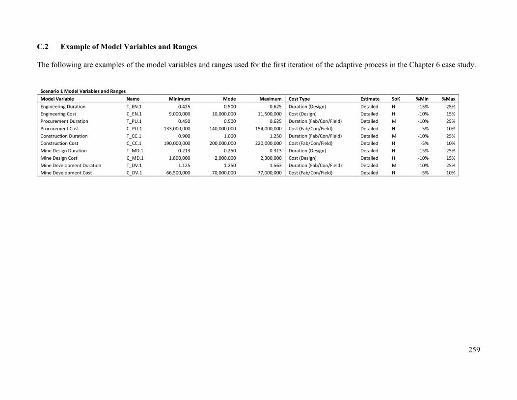
259

C.2 Example of Model Variables and Ranges

The following are examples of the model variables and ranges used for the first iteration of the adaptive process in the Chapter 6 case study.

Scenario 1 Model Variables and Ranges Model Variable Name Minimum Mode Maximum Cost Type Estimate SoK %Min %Max Engineering Duration T_EN.1 0.425 0.500 0.625 Duration (Design) Detailed H -15% 25% Engineering Cost C_EN.1 9,000,000 10,000,000 11,500,000 Cost (Design) Detailed H -10% 15% Procurement Duration T_PU.1 0.450 0.500 0.625 Duration (Fab/Con/Field) Detailed M -10% 25% Procurement Cost C_PU.1 133,000,000 140,000,000 154,000,000 Cost (Fab/Con/Field) Detailed H -5% 10% Construction Duration T_CC.1 0.900 1.000 1.250 Duration (Fab/Con/Field) Detailed M -10% 25% Construction Cost C_CC.1 190,000,000 200,000,000 220,000,000 Cost (Fab/Con/Field) Detailed H -5% 10% Mine Design Duration T_MD.1 0.213 0.250 0.313 Duration (Design) Detailed H -15% 25% Mine Design Cost C_MD.1 1,800,000 2,000,000 2,300,000 Cost (Design) Detailed H -10% 15% Mine Development Duration T_DV.1 1.125 1.250 1.563 Duration (Fab/Con/Field) Detailed M -10% 25% Mine Development Cost C_DV.1 66,500,000 70,000,000 77,000,000 Cost (Fab/Con/Field) Detailed H -5% 10%

260

Scenario 2 Model Variables and Ranges Model Variable Name Minimum Mode Maximum Cost Type Estimate SoK %Low %High Current Iteration Work Packages Drill and Assay Duration T_DA.2 0.213 0.250 0.338 Duration (Fab/Con/Field) Preliminary L -15% 35% Drill and Assay Cost C_DA.2 4,000,000 5,000,000 6,500,000 Cost (Fab/Con/Field) Preliminary L -20% 30% Alternative 1 No Change Engineering Duration T_EN.2.1 0.425 0.500 0.625 Duration (Design) Detailed H -15% 25% Engineering Cost C_EN.2.1 9,000,000 10,000,000 11,500,000 Cost (Design) Detailed H -10% 15% Procurement Duration T_PU.2.1 0.450 0.500 0.625 Duration (Fab/Con/Field) Detailed M -10% 25% Procurement Cost C_PU.2.1 133,000,000 140,000,000 154,000,000 Cost (Fab/Con/Field) Detailed H -5% 10% Construction Duration T_CC.2.1 0.900 1.000 1.250 Duration (Fab/Con/Field) Detailed M -10% 25% Construction Cost C_CC.2.1 190,000,000 200,000,000 220,000,000 Cost (Fab/Con/Field) Detailed H -5% 10% Mine Design Duration T_MD.2.1 0.213 0.250 0.313 Duration (Design) Detailed H -15% 25% Mine Design Cost C_MD.2.1 1,800,000 2,000,000 2,300,000 Cost (Design) Detailed H -10% 15% Mine Development Duration T_DV.2.1 1.125 1.250 1.563 Duration (Fab/Con/Field) Detailed M -10% 25% Mine Development Cost C_DV.2.1 66,500,000 70,000,000 77,000,000 Cost (Fab/Con/Field) Detailed H -5% 10% Alternative 2 Ore Blending Engineering Duration T_EN.2.2 0.425 0.500 0.625 Duration (Design) Detailed H -15% 25% Engineering Cost C_EN.2.2 9,000,000 10,000,000 11,500,000 Cost (Design) Detailed H -10% 15% Procurement Duration T_PU.2.2 0.450 0.500 0.625 Duration (Fab/Con/Field) Detailed M -10% 25% Procurement Cost C_PU.2.2 133,000,000 140,000,000 154,000,000 Cost (Fab/Con/Field) Detailed H -5% 10% Construction Duration T_CC.2.2 0.900 1.000 1.250 Duration (Fab/Con/Field) Detailed M -10% 25% Construction Cost C_CC.2.2 190,000,000 200,000,000 220,000,000 Cost (Fab/Con/Field) Detailed H -5% 10% Mine Design Duration T_MD.2.2 0.400 0.500 0.650 Duration (Design) Mixed M -20% 30% Mine Design Cost C_MD.2.2 3,400,000 4,000,000 4,800,000 Cost (Design) Mixed M -15% 20% Mine Development Duration T_DV.2.2 1.575 1.750 2.188 Duration (Fab/Con/Field) Mixed M -10% 25% Mine Development Cost C_DV.2.2 87,500,000 100,000,000 120,000,000 Cost (Fab/Con/Field) Mixed M -13% 20% Alternative 3 Process Changes Process Design Duration T_PD.2.3 0.188 0.250 0.338 Duration (Design) Preliminary L -25% 35% Process Design Cost C_PD.2.3 400,000 500,000 625,000 Cost (Design) Preliminary L -20% 25% Engineering Duration T_EN.2.3 0.400 0.500 0.650 Duration (Design) Mixed M -20% 30% Engineering Cost C_EN.2.3 9,350,000 11,000,000 13,200,000 Cost (Design) Mixed M -15% 20% Procurement Duration T_PU.2.3 0.450 0.500 0.625 Duration (Fab/Con/Field) Mixed M -10% 25% Procurement Cost C_PU.2.3 129,500,000 148,000,000 177,600,000 Cost (Fab/Con/Field) Mixed M -13% 20% Construction Duration T_CC.2.3 1.125 1.250 1.563 Duration (Fab/Con/Field) Mixed M -10% 25% Construction Cost C_CC.2.3 192,500,000 220,000,000 264,000,000 Cost (Fab/Con/Field) Mixed M -13% 20% Mine Design Duration T_MD.2.3 0.213 0.250 0.313 Duration (Design) Detailed H -15% 25% Mine Design Cost C_MD.2.3 1,800,000 2,000,000 2,300,000 Cost (Design) Detailed H -10% 15% Mine Development Duration T_DV.2.3 1.125 1.250 1.563 Duration (Fab/Con/Field) Detailed M -10% 25% Mine Development Cost C_DV.2.3 66,500,000 70,000,000 77,000,000 Cost (Fab/Con/Field) Detailed H -5% 10%

261

Scenario 3A Model Variables and Ranges Model Variable Name Minimum Mode Maximum Cost Type Estimate SoK %Low %High Current Iteration Work Packages Drill and Assay Duration T_DA.3A.0 0.213 0.250 0.338 Duration (Fab/Con/Field) Preliminary L -15% 35% Drill and Assay Cost C_DA.3A.0 4,000,000 5,000,000 6,500,000 Cost (Fab/Con/Field) Preliminary L -20% 30% Engineering Duration T_EN.3A.0 0.213 0.250 0.313 Duration (Design) Detailed H -15% 25% Engineering Cost C_EN.3A.0 4,500,000 5,000,000 5,750,000 Cost (Design) Detailed H -10% 15% Alternative 1 No Change Engineering Duration T_EN.3A.1 0.213 0.250 0.313 Duration (Design) Detailed H -15% 25% Engineering Cost C_EN.3A.1 4,500,000 5,000,000 5,750,000 Cost (Design) Detailed H -10% 15% Procurement Duration T_PU.3A.1 0.450 0.500 0.625 Duration (Fab/Con/Field) Detailed M -10% 25% Procurement Cost C_PU.3A.1 133,000,000 140,000,000 154,000,000 Cost (Fab/Con/Field) Detailed H -5% 10% Construction Duration T_CC.3A.1 0.900 1.000 1.250 Duration (Fab/Con/Field) Detailed M -10% 25% Construction Cost C_CC.3A.1 190,000,000 200,000,000 220,000,000 Cost (Fab/Con/Field) Detailed H -5% 10% Mine Design Duration T_MD.3A.1 0.213 0.250 0.313 Duration (Design) Detailed H -15% 25% Mine Design Cost C_MD.3A.1 1,800,000 2,000,000 2,300,000 Cost (Design) Detailed H -10% 15% Mine Development Duration T_DV.3A.1 1.125 1.250 1.563 Duration (Fab/Con/Field) Detailed M -10% 25% Mine Development Cost C_DV.3A.1 66,500,000 70,000,000 77,000,000 Cost (Fab/Con/Field) Detailed H -5% 10% Alternative 2 Ore Blending Engineering Duration T_EN.3A.2 0.213 0.250 0.313 Duration (Design) Detailed H -15% 25% Engineering Cost C_EN.3A.2 4,500,000 5,000,000 5,750,000 Cost (Design) Detailed H -10% 15% Procurement Duration T_PU.3A.2 0.450 0.500 0.625 Duration (Fab/Con/Field) Detailed M -10% 25% Procurement Cost C_PU.3A.2 133,000,000 140,000,000 154,000,000 Cost (Fab/Con/Field) Detailed H -5% 10% Construction Duration T_CC.3A.2 0.900 1.000 1.250 Duration (Fab/Con/Field) Detailed M -10% 25% Construction Cost C_CC.3A.2 190,000,000 200,000,000 220,000,000 Cost (Fab/Con/Field) Detailed H -5% 10% Mine Design Duration T_MD.3A.2 0.375 0.500 0.675 Duration (Design) Detailed L -25% 35% Mine Design Cost C_MD.3A.2 3,200,000 4,000,000 5,000,000 Cost (Design) Detailed L -20% 25% Mine Development Duration T_DV.3A.2 1.488 1.750 2.363 Duration (Fab/Con/Field) Mixed L -15% 35% Mine Development Cost C_DV.3A.2 87,500,000 100,000,000 120,000,000 Cost (Fab/Con/Field) Mixed M -13% 20% Alternative 3 Process Changes Process Design Duration T_PD.3A.3 0.188 0.250 0.338 Duration (Design) Preliminary L -25% 35% Process Design Cost C_PD.3A.3 400,000 500,000 625,000 Cost (Design) Preliminary L -20% 25% Engineering Duration T_EN.3A.3 0.200 0.250 0.325 Duration (Design) Mixed M -20% 30% Engineering Cost C_EN.3A.3 5,100,000 6,000,000 7,200,000 Cost (Design) Mixed M -15% 20% Procurement Duration T_PU.3A.3 0.450 0.500 0.625 Duration (Fab/Con/Field) Mixed M -10% 25% Procurement Cost C_PU.3A.3 129,500,000 148,000,000 177,600,000 Cost (Fab/Con/Field) Mixed M -13% 20% Construction Duration T_CC.3A.3 1.125 1.250 1.563 Duration (Fab/Con/Field) Mixed M -10% 25% Construction Cost C_CC.3A.3 192,500,000 220,000,000 264,000,000 Cost (Fab/Con/Field) Mixed M -13% 20% Mine Design Duration T_MD.3A.3 0.213 0.250 0.313 Duration (Design) Detailed H -15% 25% Mine Design Cost C_MD.3A.3 1,800,000 2,000,000 2,300,000 Cost (Design) Detailed H -10% 15% Mine Development Duration T_DV.3A.3 1.125 1.250 1.563 Duration (Fab/Con/Field) Detailed M -10% 25% Mine Development Cost C_DV.3A.3 66,500,000 70,000,000 77,000,000 Cost (Fab/Con/Field) Detailed H -5% 10%

262

Scenario 3B Model Variables and Ranges Model Variable Name Minimum Mode Maximum Cost Type Estimate SoK %Low %High Current Iteration Work Packages Drill and Assay Duration T_DA.3B.0 0.213 0.250 0.338 Duration (Fab/Con/Field) Preliminary L -15% 35% Drill and Assay Cost C_DA.3B.0 4,000,000 5,000,000 6,500,000 Cost (Fab/Con/Field) Preliminary L -20% 30% Mine Design Duration T_MD.3B.0 0.213 0.250 0.313 Duration (Design) Detailed H -15% 25% Mine Design Cost C_MD.3B.0 1,800,000 2,000,000 2,300,000 Cost (Design) Detailed H -10% 15% Alternative 1 No Change Engineering Duration T_EN.3B.1 0.425 0.500 0.625 Duration (Design) Detailed H -15% 25% Engineering Cost C_EN.3B.1 9,000,000 10,000,000 11,500,000 Cost (Design) Detailed H -10% 15% Procurement Duration T_PU.3B.1 0.450 0.500 0.625 Duration (Fab/Con/Field) Detailed M -10% 25% Procurement Cost C_PU.3B.1 133,000,000 140,000,000 154,000,000 Cost (Fab/Con/Field) Detailed H -5% 10% Construction Duration T_CC.3B.1 0.900 1.000 1.250 Duration (Fab/Con/Field) Detailed M -10% 25% Construction Cost C_CC.3B.1 190,000,000 200,000,000 220,000,000 Cost (Fab/Con/Field) Detailed H -5% 10% Mine Development Duration T_DV.3B.1 1.125 1.250 1.563 Duration (Fab/Con/Field) Detailed M -10% 25% Mine Development Cost C_DV.3B.1 66,500,000 70,000,000 77,000,000 Cost (Fab/Con/Field) Detailed H -5% 10% Alternative 2 Ore Blending Engineering Duration T_EN.3B.2 0.425 0.500 0.625 Duration (Design) Detailed H -15% 25% Engineering Cost C_EN.3B.2 9,000,000 10,000,000 11,500,000 Cost (Design) Detailed H -10% 15% Procurement Duration T_PU.3B.2 0.450 0.500 0.625 Duration (Fab/Con/Field) Detailed M -10% 25% Procurement Cost C_PU.3B.2 133,000,000 140,000,000 154,000,000 Cost (Fab/Con/Field) Detailed H -5% 10% Construction Duration T_CC.3B.2 0.900 1.000 1.250 Duration (Fab/Con/Field) Detailed M -10% 25% Construction Cost C_CC.3B.2 190,000,000 200,000,000 220,000,000 Cost (Fab/Con/Field) Detailed H -5% 10% Mine Design Duration T_MD.3B.2 0.188 0.250 0.338 Duration (Design) Detailed L -25% 35% Mine Design Cost C_MD.3B.2 1,600,000 2,000,000 2,500,000 Cost (Design) Detailed L -20% 25% Mine Development Duration T_DV.3B.2 1.488 1.750 2.363 Duration (Fab/Con/Field) Mixed L -15% 35% Mine Development Cost C_DV.3B.2 87,500,000 100,000,000 120,000,000 Cost (Fab/Con/Field) Mixed M -13% 20% Alternative 3 Process Changes Process Design Duration T_PD.3B.3 0.188 0.250 0.338 Duration (Design) Preliminary L -25% 35% Process Design Cost C_PD.3B.3 400,000 500,000 625,000 Cost (Design) Preliminary L -20% 25% Engineering Duration T_EN.3B.3 0.400 0.500 0.650 Duration (Design) Mixed M -20% 30% Engineering Cost C_EN.3B.3 9,350,000 11,000,000 13,200,000 Cost (Design) Mixed M -15% 20% Procurement Duration T_PU.3B.3 0.450 0.500 0.625 Duration (Fab/Con/Field) Mixed M -10% 25% Procurement Cost C_PU.3B.3 129,500,000 148,000,000 177,600,000 Cost (Fab/Con/Field) Mixed M -13% 20% Construction Duration T_CC.3B.3 1.125 1.250 1.563 Duration (Fab/Con/Field) Mixed M -10% 25% Construction Cost C_CC.3B.3 192,500,000 220,000,000 264,000,000 Cost (Fab/Con/Field) Mixed M -13% 20% Mine Development Duration T_DV.3B.3 1.125 1.250 1.563 Duration (Fab/Con/Field) Detailed M -10% 25% Mine Development Cost C_DV.3B.3 66,500,000 70,000,000 77,000,000 Cost (Fab/Con/Field) Detailed H -5% 10%

263

Scenario 3C Model Variables and Ranges Model Variable Name Minimum Mode Maximum Cost Type Estimate SoK %Low %High Current Iteration Work Packages Drill and Assay Duration T_DA.3C.0 0.213 0.250 0.338 Duration (Fab/Con/Field) Preliminary L -15% 35% Drill and Assay Cost C_DA.3C.0 4,000,000 5,000,000 6,500,000 Cost (Fab/Con/Field) Preliminary L -20% 30% Process Design Duration T_PD.3C.0 0.188 0.250 0.338 Duration (Design) Preliminary L -25% 35% Process Design Cost C_PD.3C.0 400,000 500,000 625,000 Cost (Design) Preliminary L -20% 25% Alternative 1 No Change Engineering Duration T_EN.3C.1 0.425 0.500 0.625 Duration (Design) Detailed H -15% 25% Engineering Cost C_EN.3C.1 9,000,000 10,000,000 11,500,000 Cost (Design) Detailed H -10% 15% Procurement Duration T_PU.3C.1 0.450 0.500 0.625 Duration (Fab/Con/Field) Detailed M -10% 25% Procurement Cost C_PU.3C.1 133,000,000 140,000,000 154,000,000 Cost (Fab/Con/Field) Detailed H -5% 10% Construction Duration T_CC.3C.1 0.900 1.000 1.250 Duration (Fab/Con/Field) Detailed M -10% 25% Construction Cost C_CC.3C.1 190,000,000 200,000,000 220,000,000 Cost (Fab/Con/Field) Detailed H -5% 10% Mine Design Duration T_MD.3C.1 0.213 0.250 0.313 Duration (Design) Detailed H -15% 25% Mine Design Cost C_MD.3C.1 1,800,000 2,000,000 2,300,000 Cost (Design) Detailed H -10% 15% Mine Development Duration T_DV.3C.1 1.125 1.250 1.563 Duration (Fab/Con/Field) Detailed M -10% 25% Mine Development Cost C_DV.3C.1 66,500,000 70,000,000 77,000,000 Cost (Fab/Con/Field) Detailed H -5% 10% Alternative 2 Ore Blending Engineering Duration T_EN.3C.2 0.425 0.500 0.625 Duration (Design) Detailed H -15% 25% Engineering Cost C_EN.3C.2 9,000,000 10,000,000 11,500,000 Cost (Design) Detailed H -10% 15% Procurement Duration T_PU.3C.2 0.450 0.500 0.625 Duration (Fab/Con/Field) Detailed M -10% 25% Procurement Cost C_PU.3C.2 133,000,000 140,000,000 154,000,000 Cost (Fab/Con/Field) Detailed H -5% 10% Construction Duration T_CC.3C.2 0.900 1.000 1.250 Duration (Fab/Con/Field) Detailed M -10% 25% Construction Cost C_CC.3C.2 190,000,000 200,000,000 220,000,000 Cost (Fab/Con/Field) Detailed H -5% 10% Mine Design Duration T_MD.3C.2 0.375 0.500 0.675 Duration (Design) Detailed L -25% 35% Mine Design Cost C_MD.3C.2 3,200,000 4,000,000 5,000,000 Cost (Design) Detailed L -20% 25% Mine Development Duration T_DV.3C.2 1.488 1.750 2.363 Duration (Fab/Con/Field) Mixed L -15% 35% Mine Development Cost C_DV.3C.2 87,500,000 100,000,000 120,000,000 Cost (Fab/Con/Field) Mixed M -13% 20% Alternative 3 Process Changes Engineering Duration T_EN.3C.3 0.400 0.500 0.650 Duration (Design) Mixed M -20% 30% Engineering Cost C_EN.3C.3 9,350,000 11,000,000 13,200,000 Cost (Design) Mixed M -15% 20% Procurement Duration T_PU.3C.3 0.450 0.500 0.625 Duration (Fab/Con/Field) Mixed M -10% 25% Procurement Cost C_PU.3C.3 129,500,000 148,000,000 177,600,000 Cost (Fab/Con/Field) Mixed M -13% 20% Construction Duration T_CC.3C.3 1.125 1.250 1.563 Duration (Fab/Con/Field) Mixed M -10% 25% Construction Cost C_CC.3C.3 192,500,000 220,000,000 264,000,000 Cost (Fab/Con/Field) Mixed M -13% 20% Mine Design Duration T_MD.3C.3 0.213 0.250 0.313 Duration (Design) Detailed H -15% 25% Mine Design Cost C_MD.3C.3 1,800,000 2,000,000 2,300,000 Cost (Design) Detailed H -10% 15% Mine Development Duration T_DV.3C.3 1.125 1.250 1.563 Duration (Fab/Con/Field) Detailed M -10% 25% Mine Development Cost C_DV.3C.3 66,500,000 70,000,000 77,000,000 Cost (Fab/Con/Field) Detailed H -5% 10%

264

Scenario 4 Model Variable Name Minimum Mode Maximum Cost Type Estimate SoK %Low %High Current Iteration Work Packages Drill and Assay Duration T_DA.4.0 0.213 0.250 0.338 Duration (Fab/Con/Field) Preliminary L -15% 35% Drill and Assay Cost C_DA.4.0 4,000,000 5,000,000 6,500,000 Cost (Fab/Con/Field) Preliminary L -20% 30% Process Design Duration T_PD.4.0 0.188 0.250 0.338 Duration (Design) Preliminary L -25% 35% Process Design Cost C_PD.4.0 400,000 500,000 625,000 Cost (Design) Preliminary L -20% 25% Mine Design Duration T_MD.4.0 0.213 0.250 0.313 Duration (Design) Detailed H -15% 25% Mine Design Cost C_MD.4.0 1,800,000 2,000,000 2,300,000 Cost (Design) Detailed H -10% 15% Engineering Duration T_EN.4.0 0.213 0.250 0.313 Duration (Design) Detailed H -15% 25% Engineering Cost C_EN.4.0 4,500,000 5,000,000 5,750,000 Cost (Design) Detailed H -10% 15% Alternative 1 No Change Engineering Duration T_EN.4.1 0.213 0.250 0.313 Duration (Design) Detailed H -15% 25% Engineering Cost C_EN.4.1 4,500,000 5,000,000 5,750,000 Cost (Design) Detailed H -10% 15% Procurement Duration T_PU.4.1 0.450 0.500 0.625 Duration (Fab/Con/Field) Detailed M -10% 25% Procurement Cost C_PU.4.1 133,000,000 140,000,000 154,000,000 Cost (Fab/Con/Field) Detailed H -5% 10% Construction Duration T_CC.4.1 0.900 1.000 1.250 Duration (Fab/Con/Field) Detailed M -10% 25% Construction Cost C_CC.4.1 190,000,000 200,000,000 220,000,000 Cost (Fab/Con/Field) Detailed H -5% 10% Mine Development Duration T_DV.4.1 1.125 1.250 1.563 Duration (Fab/Con/Field) Detailed M -10% 25% Mine Development Cost C_DV.4.1 66,500,000 70,000,000 77,000,000 Cost (Fab/Con/Field) Detailed H -5% 10% Alternative 2 Ore Blending Engineering Duration T_EN.4.2 0.213 0.250 0.313 Duration (Design) Detailed H -15% 25% Engineering Cost C_EN.4.2 4,500,000 5,000,000 5,750,000 Cost (Design) Detailed H -10% 15% Procurement Duration T_PU.4.2 0.450 0.500 0.625 Duration (Fab/Con/Field) Detailed M -10% 25% Procurement Cost C_PU.4.2 133,000,000 140,000,000 154,000,000 Cost (Fab/Con/Field) Detailed H -5% 10% Construction Duration T_CC.4.2 0.900 1.000 1.250 Duration (Fab/Con/Field) Detailed M -10% 25% Construction Cost C_CC.4.2 190,000,000 200,000,000 220,000,000 Cost (Fab/Con/Field) Detailed H -5% 10% Mine Design Duration T_MD.4.2 0.188 0.250 0.338 Duration (Design) Detailed L -25% 35% Mine Design Cost C_MD.4.2 1,600,000 2,000,000 2,500,000 Cost (Design) Detailed L -20% 25% Mine Development Duration T_DV.4.2 1.488 1.750 2.363 Duration (Fab/Con/Field) Mixed L -15% 35% Mine Development Cost C_DV.4.2 87,500,000 100,000,000 120,000,000 Cost (Fab/Con/Field) Mixed M -13% 20% Alternative 3 Process Changes Engineering Duration T_EN.4.3 0.200 0.250 0.325 Duration (Design) Mixed M -20% 30% Engineering Cost C_EN.4.3 5,100,000 6,000,000 7,200,000 Cost (Design) Mixed M -15% 20% Procurement Duration T_PU.4.3 0.450 0.500 0.625 Duration (Fab/Con/Field) Mixed M -10% 25% Procurement Cost C_PU.4.3 129,500,000 148,000,000 177,600,000 Cost (Fab/Con/Field) Mixed M -13% 20% Construction Duration T_CC.4.3 1.125 1.250 1.563 Duration (Fab/Con/Field) Mixed M -10% 25% Construction Cost C_CC.4.3 192,500,000 220,000,000 264,000,000 Cost (Fab/Con/Field) Mixed M -13% 20% Mine Development Duration T_DV.4.3 1.125 1.250 1.563 Duration (Fab/Con/Field) Detailed M -10% 25% Mine Development Cost C_DV.4.3 66,500,000 70,000,000 77,000,000 Cost (Fab/Con/Field) Detailed H -5% 10%

adaptive risk management in mining project development: a ...

Documents

Transcript of adaptive risk management in mining project development: a ...