Auto-Contractive Maps: An Artificial Adaptive System for Data Mining. An Application to Alzheimer...

Current Alzheimer Research, 2008, 5, 481-498 481

1567-2050/08 $55.00+.00 ©2008 Bentham Science Publishers Ltd.

Auto-Contractive Maps: An Artificial Adaptive System for Data Mining. An Application to Alzheimer Disease

1

Massimo Buscema1,*

, Enzo Grossi2, Dave Snowdon

3 and Piero Antuono

4

1Semeion Research Center, Rome, Italy;

2Bracco Medical Affairs Europe,Via E. Folli 50, 20134 Milan, Italy;

3Sanders-

Brown Center on Aging, Department of Preventive Medicine, College of Medicine, University of Kentucky, Lexington,

KY; USA; 4The Medical College of Wisconsin, 9200 West Wisconsin Avenue, Milwaukee, WI, USA

Abstract: This article presents a new paradigm of Artificial Neural Networks (ANNs): the Auto-Contractive Maps (Auto-

CM). The Auto-CM differ from the traditional ANNs under many viewpoints: the Auto-CM start their learning task with-

out a random initialization of their weights, they meet their convergence criterion when all their output nodes become

null, their weights matrix develops a data driven warping of the original Euclidean space, they show suitable topological

properties, etc. Further two new algorithms, theoretically linked to Auto-CM are presented: the first one is useful to evalu-

ate the complexity and the topological information of any kind of connected graph: the H Function is the index to measure

the global hubness of the graph generated by the Auto-CM weights matrix. The second one is named Maximally Regular

Graph (MRG) and it is an development of the traditionally Minimum Spanning Tree (MST). Finally, Auto-CM and MRG,

with the support of the H Function, are applied to a real complex dataset about Alzheimer disease: this data come from the

very known Nuns Study, where variables measuring the abilities of normal and Alzheimer subject during their lifespan

and variables measuring the number of the plaques and of the tangles in their brain after their death.

The example of the Alzheimer data base is extremely useful to figure out how this new approach can help to re design

bottom-up the overall structure of factors related to a complex disease like this.

Keywords: Artificial neural networks, contractive maps, artificial adaptive systems, theory of graph, minimum spanning tree, Alzheimer disease, nun study.

1. AUTO-CONTRACTIVE MAPS, H FUNCTION AND MAXIMALLY REGULAR GRAPH

1.1. Introduction

Investigating the pattern of correlations among large numbers of variables in large databases is certainly a quite difficult task, that is seriously demanding in both computa-tional time and capacity. The statistically-oriented literature has developed a variety of methods with different power and usability, all of which, however, share a few basic problems, among which the most outstanding are: the nature of the a-priori assumptions that have to be made on the data-generating process, the near impossibility to compute all the joint probabilities among the vast number of possible cou-ples and n-tuples that are in principle necessary to recon-struct the underlying process’ probability law, and the diffi-culty of organizing the output in an easily grasped, ready-to-access format for the non-technical analyst. The consequence of the first two weaknesses is the fact that when analyzing poorly understood problems characterized by heterogeneous sets of potentially relevant variables, traditional methods can become very unreliable when not unusable. The consequence of the last one is that, also in the cases where traditional

methods manage to provide a sensible output, its statement and implications can be so articulated to become practically un-useful or, even worse, easily misunderstood.

In this paper, we introduce a new methodology based on an Artificial Neural Network (ANN) architecture, the Auto Contractive Map (AutoCM), which allows for basic im-provements in both robustness of use in badly specified and/or computationally demanding problems, and output usability and intelligibility. In particular, AutoCMs ‘spatial-ize’ the correlation among variables by constructing a suit-able embedding space where a visually transparent and cog-nitively natural notion such as ‘closeness’ among variables reflects accurately their associations. Through suitable opti-mization techniques that will be introduced and discussed in detail in what follows, ‘closeness’ can be converted into a compelling graph-theoretic representation that picks all and only the relevant correlations and organizes them into a co-herent picture. Such representation is not actually con-structed through some form of cumbersome aggregation of two-by-two associations between couples of variables, but rather by building a complex global picture of the whole pattern of variation. Moreover, it fully exploits the topologi-

__________________________________ 1

The architecture of Auto Contractive Map (equations, topology and parameters) was ideated by Massimo Buscema at Semeion Research Center from 2000 to 2007. Auto Contrac-

tive Map is implemented in Buscema[2002], Buscema[2007] and Massini[2007b].

The Pruning Algorithm was ideated by Giulia Massini at Semeion Research Center in 2006. The Pruning Algorithm is implemented in Massini[2007a] and Buscema[2008].

The H Function was ideated by Massimo Buscema at Semeion Research Center in 2007. The H Function is implemented in Buscema[2008].

The Maximally Regular Graph (M.R.G.) was ideated by Massimo Buscema at Semeion Research Center in 2007. The M.R.G. is implemented in Buscema[2008].

*Address correspondence to this author at the Semeion Research Center, Rome, Italy; Bracco Medical Affairs Europe,Via E. Folli 50, 20134 Milan, Italy; E-mail: [email protected]

482 Current Alzheimer Research, 2008, Vol. 5, No. 5 Buscema et al.

cal meaningfulness of graph-theoretic representations in that actual paths connecting nodes (variables) in the representa-tion carry a definite meaning in terms of logical interdepend-ence in explaining the data set’s variability. We are aware of the fact that these techniques are novel and therefore not entirely understood so far in all of their properties and impli-cations, and that further research is called for to explore them. But at the same time we are convinced that their actual performance in the context of well-defined, well understood problems provides an encouraging test to proceed in this direction.

1.2. Learning Equations

The Auto Contractive Map (CM) presents a three layers architecture: an Input layer, where the signal is captured from the environment, an Hidden layer, where the signal is modulated inside the CM, and an Output layer by which the CM influences the environment according to the stimuli pre-viously received

1 (see Fig. (1)) [1,2].

Each layer is composed by N units. Then the whole CM is composed by 3N units. The connections between the Input layer and the Hidden layer are Mono-dedicated, whereas the ones between the Hidden layer and the Output layer are at maximum gradient. Therefore, in relation to the units the number of the connections Nc, is given by: Nc = N (N + 1).

Fig. (1). An example of a AutoCM with N=4

All the connections of CM may be initialized both by equal values and by values at random. The best practice is to initialize all the connections with the same positive value, close to zero.

The learning algorithm of CM may be summarized in four orderly steps:

1. Signal Transfer from the Input into the Hidden layer;

2. Adaptation of the connections value between the Input layer and the Hidden layer; *

3. Signal Transfer from the Hidden layer into the Output layer; *

4. Adaptation of the connections value between the Hidden layer and the Output layer.

(*): step 2 and 3 may take place in parallel.

We define as m[s]

the units of the Input layer (sensors), scaled between 0 and 1, as m

[h] the ones of the Hidden layer

and as m[t ]

the ones of the Output layer (system target). We

1 Buscema M., Squashing Theory and Contractive Map Network, Semeion Technical

Paper #32, Rome, 2007.

define v the vector of monodedicated connections , w the matrix of the connections between Hidden layer and Output layer, and n the discrete time of the weights evolution, or rather n is the number of cycles of elaboration that, starting from zero increases itself of a unit at each successive cycle:

Nn .

The signal forward transfer equations and the learning ones are four:

a. Signal transfer from the Input to the Hidden:

mi(n )

h[ ] = mis[ ] 1

vi(n )

C (1)

where C = Positive real number not lower than 1, named

Contractive Factor, and where (n) subscript has been omitted

from input layer units, these being constant at every elabora-

tion cycle.

b. Adaptation of the connections )(niv through the

( )niv trapping the energy difference generated by the equa-tion (1):

vi( n )

= mi

sm

i( n )

h( ) 1v

i( n )

C ; (2)

( 1) ( ) ( )n n ni i iv v v+

= + ; (3)

c. Signal transfer from the Hidden to the Output:

( )

( ) ( )

,[ ] 1 ;n

n n

Ni jh

i j

j

wNet m

C= (4)

( )

( ) ( )

[ ] [ ] 1n

n n

it h

i i

Netm m

C= . (5)

d. Adaptation of the connections ( ), ni jw through the

( ), ni jw

trapping the energy differences generated by the equation

(5):

wi, j

( n )

= mi( n )

[h] mi( n )

[t ]( ) 1w

i, j( n )

Cm

j( n )

[h] ; (6)

( 1) ( ) ( ), , ,n n ni j i j i jw w w+

= + (7)

Even a cursory comparison of (1) and (5) and (2-3), (6-7), respectively, clearly shows how both steps of the signal transfer process are guided by the same (contraction) princi-ple, and likewise for the two weight adaptation steps (for which we could speak of an energy entrapment principle).

Notice how the term ( )

[ ]

n

h

jm in (6) makes the change in the

connection ( ), ni jw proportional to the quantity of energy lib-

erated by node ( )

[ ]

n

h

im in favor of node ( )

[ ]

n

t

im . The whole learn-

ing process, which essentially consists of a progressive ad-

justment of the connections aimed at the global minimization

of energy, may be seen as a complex juxtaposition of phases

of acceleration and deceleration of velocities of the learning

signals (adaptations ( ), ni jw and

( )niv ) inside the ANN con-

��

��

��

��

�

�

Auto-Contractive Maps Current Alzheimer Research, 2008, Vol. 5, No. 5 483

nection matrix. To get a clearer understanding of this feature

of the AutoCM learning mechanics, begin by considering its

convergence condition:

limn

vi( n )

= C (8)

Indeed, when v

i( n )

= C , then ( )

0niv = (according to eq

2), and ( )

[ ] 0n

h

jm = (according to eq 1) and, conse-

quently,( ), 0ni jw = (as from eq 6): the AutoCM then con-

verges.

There are, moreover, four variables that play a key role in the learning mechanics of AutoCM. Specifically,

1.

i( n )

is the contraction factor of the first layer of AutoCM

weights:

( )

( )1

n

n

i

i

v

C=

As it is apparent from (1), the parameter C modulates the transmission of the Input signal into the Hidden layer by ‘squeezing’ it for given values of the connections; the actual extent of the squeeze is indeed controlled by the value of C, thereby explaining its interpretation as the contraction pa-rameter. Clearly, the choice of C and the initialization of the connection weights must be such that the contraction factor is a number always falling within the [0 , 1] range, and de-creasing at every processing cycle n, to become infinitesimal as n diverges.

2.

i, j( n )

is, analogously, the contraction factor of the second

layer of AutoCM weights which, once again given the ini-

tialization choice, falls strictly within the unit interval:

C

wn

n

ji

ji

)(

)(

,

, 1=

As for the previous layer, the value of the contraction factor is modulated by the contraction parameter C.

3. )(ni is the difference between the Hidden and the Input

nodes:

][][

)()(

h

i

s

ii nnmm=

It is a real function of n, and it always takes positive, decreasing values in view of the contractive character of the signal transfer process.

4. )(ni is, likewise, the difference between the Output and

the Hidden nodes:

][][

)()()(

t

i

h

ii nnnmm=

It is, by the same token, a real function with positive val-ues, decreasing in n.

The second step to gain insight into the AutoCM learning

mechanics is to demonstrate how, during the AutoCM learn-

ing phase, ( )niv describes a parabola arc, always lying in the

positive orthant. To see this, re-write equation (2) as:

vi( n )

= mi

sm

i

s1

vi( n )

C1

vi( n )

C=

= mi

sv

i( n )

C1

vi( n )

C

(2a)

Remembering how )(ni was defined, we can write

)(1)(

ni

i

C

vn

= and then further re-write (2a) as a function

of the contraction factor )(ni :

[ ]

[ ]

( ) ( ) ( )

( ) ( )

(1 ) (1 (1 ))

(1 )

n n n

n n

s

i i i i

s

i i i

v m

m

= =

=

(2b)

Keeping in mind the definition of )(ni , and letting the

values of the input layer units decrease along the unit inter-

val, one can easily check that the )(niv parabola arc (2b)

meets the following condition:

)()()(0

nnn iii Cv << (2c)

Equation (2c) tells us that the adaptation of the connec-

tions between the Input and Hidden layers, ( )niv , will be

always smaller than the adaptation that v

i( n )

needs to reach up

C. Actually, )()()()()1( nnnnn iiiii vCCvvv +=+=

+,

but from (2c) we know that 0)()( nn ii Cv , which

proves our claim. As a consequence, )(niv will never exceed

C. However, the convergence condition requires that

Cvni

n=

)(lim , which in turn implies the following:

( )

lim 0i nn

= , [ ] 0lim

)(

=h

n nim ,

[ ] 0lim)(

=t

n nim , (8)

[ ]s

in

mni

=)(

lim , and 0lim)(

=nin

In view of the contractive character of the signal trans-mission process at both of the AutoCM’s layer levels, com-bining equations (1) and (5) we can also write:

[ ]s

i

h

i

t

i mmmnn

][][

)()(; (1-5)

and in particular, we can reformulate them as follows:

)()(

][][

nn i

s

i

h

i mm = (1a)


and

=C

Netmm n

nn

i

i

s

i

t

i

)(

)()(1][][

(5a)

We are now in the position to clarify the relationship

between

vi( n )

and wi, j

( n )

. From equation (1-5), we can

stipulate:

)()(

][][

nn i

s

i

h

i mm = (1b)

where

i( n )

is a small positive real number;

and

)()()(

][][

nnn i

h

i

t

i mm = (5b)

where )(ni is another small positive real number. As already

remarked, such small positive numbers must become close to

0 as n diverges. We can also write

)()()()(

][][

nnn ii

s

i

t

i mm += . (5c)

At this point, we can easily reformulate equation (2) as:

vi( n )

= mi

sm

i( n )

h( ) 1v

i( n )

C =

i( n )

i( n )

(2d)

And, likewise, equation (6) as:

wi, j

( n )

= mi( n )

hm

i( n )

t( ) 1w

i, j( n )

C m

j( n )

h=

= i( n )

i, j( n )

mj

s

i( n )

(6b)

noting that

lim wi, j

( n )

= 0

0

(6e)

Plugging (6b) into (7) and remembering the definition of

the contraction factor ( ), ni j yields:

w

i, j( n+1)

= C 1i, j

( n )( ) +

i( n )

i( n )

mj

s

i( n )

(7a)

Finally, from (7a) and (8), we can conclude that:

)1(lim)()( ,, nn jiji

nCw = (7b)

In a nutshell, the learning mechanics of the AutoCM

boils down to the following. At the beginning of the training,

the Input and Hidden units will be very similar (see equation

(1)), and, consequently, ( )niv will be very small (see equa-

tion (2d)), while for the same reason )(ni (see its definition

above) at the beginning will be very big and ( ), ni jw bigger

than ( )niv (see equations (2d) and (6b)). During the training,

while v

i( n )

rapidly increases as the processing cycles n pile

up, m

i( n )

[h] decreases, and so do accordingly

)(ni and )(ni .

Consequently, ( ), ni jw rolls along a downward slope,

whereas ( )niv slows down the pace of its increase. When

)(ni becomes close to zero, this means that m

i( n )

[h] is now

only slightly bigger than ( )

[ ]

n

t

im (see equation (5b)). ( )niv is

accordingly getting across the global maximum of the equa-

tion [ ])()()(

)1(nnn ii

s

ii mv = , so once the critical point has

been hit, ( )niv will in turn begin its descent toward zero.

1.3. Auto CM: Theoretical Consideration

Auto Contractive Maps do not behave as a regular ANN:

a. They learn also starting from all connections set up with the same values. So they do not suffer the problem of the symmetric connections.

b. During training, they develop for each connection only positive values. Therefore, Auto CM do not present in-hibitory relations among nodes, but only different strengths of excitatory connections.

c. Auto CM can learn also in hard conditions, that is, when the connections of the main diagonal of the second con-nections matrix are removed. When the learning process is organized in this way, Auto CM seems to find a spe-cific relationships between each variable and any other. Consequently, from an experimental point of view, it seems that the ranking of its connections matrix is equal to the ranking of the joint probability between each vari-able and the others.

d. After learning process, any input vector, belonging to the training set, will generate a null output vector. So, the energy minimization of the training vectors is repre-sented by a function trough which the trained connec-tions absorb completely the input training vectors. Auto CM seems to learn to transform itself in a dark body.

e. At the end of the training phase ( 0, =jiw ), all the components of the weights vector v reach up the same value:

( )lim

nin

v C= . (8)

The matrix w, then, represents the CM knowledge about all the dataset.

It is possible to transform the w matrix also in probabilis-tic joint association among the variables m:

;

1

,

,

,

=

=N

j

ji

ji

ji

w

wp (9)


1)( ,

][==

N

i

ji

s

j pmP (10)

The new matrix p can be read as the probability of transi-tion from any state-variable to anyone else:

ji

s

j

t

i pmmP ,

][][ )( = . (11)

g. At the same time the matrix w may be transformed into a non Euclidean distance metric (semi-metric), when we train the CM with the main diagonal of the w matrix fixed at value N.

Now, if we consider N as a limit value for all the weights of the w matrix, we can write:

jiji wNd ,, = (12)

The new matrix d is also a squared symmetric matrix where the main diagonal represents the zero distance be-tween each variable from itself.

1.4. Auto CM and Minimum Spanning Tree

Equation (12) transforms the squared weights matrix of Auto CM into a squared matrix of distances among nodes. Each distance between a pair of node becomes, conse-quently, the weighted edge between these pair of nodes.

At this point, the matrix d may be analyzed trough the graph theory.

The Minimum Spanning Tree problem is defined as fol-lows: find an acyclic subset T of E that connects all of the vertices in the graph and whose total weight is minimized, where the total weight is given by

1

, ,

0 1

( ) ,N N

i j i j

i j i

d T d d= = +

= . (13)

T is called spanning tree, and MST is the T with the mini-mum sum of its edges weighted.

{ ( )}kMst Min d T= . (14)

Given a undirected Graph G, representing a d matrix of

distances, with V vertices, completely linked each other, the

total number of their edges (E) is:

( 1)

2

V VE = ; (15)

And the number of its possible tree is:

2VT V= . (16)

Kruskal in the 1956 found out an algorithm able to de-terminate the MST of any undirected graph in a quadratic number of steps, in the worse case [3]. Obviously, the Kruskal algorithm generates one of the possible MST. In fact in a weighted graph more than one MST are possible.

From conceptual point of view the MST represents the energy minimization state of a structure. In fact, if we con-sider the atomic elements of a structure as vertices of a graph

and the strength among them as the weight of each edge, linking a pair of vertex, the MST represents the minimum of energy needed because all the elements of the structure con-tinue to stay together.

In a closed system, all the components tend to minimize the overall energy. So the MST, in specific situations, can represent the most probable state where a system tends to.

To define the MST of a undirected graph, each edge of the graph has to be weighted. The equation (12) shows a way to weight each edge whose nodes are the variables of a dataset and whose weights of a trained AutoCM provides the metrics.

Obviously, it is possible to use any kind of AutoAssocia-tive ANN or any kind of Linear Auto-Associator to generate a weight matrix among the variables of a assigned dataset. But it is hard to train a two layer AutoAssociative Back Propagation with the weights main diagonal fixed (to avoid variables auto-correlation) [4-9]. In the most of the cases, the Root Mean Square Error stops to decrease after few epochs. Especially when the orthogonally of the records increase. And that is usual when it is necessary to weight the distance among the records of the assigned dataset. In this case, in fact, it is necessary to train the transposed matrix of the as-signed dataset.

By the way, if a Linear Auto-Associator is used, all the non linear association among variables will be lost.

So, actually, AutoCM seems to be the best choice to compute a complete and a non linear matrix of weights among variables or among records of any assigned dataset.

1.5. The Graph Complexity: the H Function

This degree of protection in a graph defines the rank of centrality of each node within the graph, when an iterative pruning algorithm is applied to the graph.

This algorithm was found and applied for the first time as a global indicator for a graph complexity by Giulia Massini at Semeion Research Center in 2006

2 [2].

Pruning Algorithm

Rank=0;

Do

{

Rank++;

Consi-der_All_Nodes_with_The_Minimum_Number_of_Links ();

Delete_These_Links();

Assign_a_Rank_To_All_Nodes_Without_Link(Rank);

Update_The_New_Graph();

Check_Number_of_Links();

} while at_least_a _link_is_present;




Higher the rank of a node, bigger is the centrality of its position within the graph. The latest nodes to be pruned are also the kernel nodes of the graph.

The pruning algorithm can be used also to define the quantity of graph complexity of any graph.

In fact, if we assume μ as the mean number of nodes

without any link in each iteration, during the pruning algo-

rithm, we can write the Hubness Index, 0H , of a graph with

N nodes as:

0 0

1; 0 2;H H

A

μ= < < (17)

where: 1

;M

i

i

ANd

M Mμ = = =

P

j

jTGSP

;1

A = number

of links of the graph (N-1 for tree graphs); M = number of

iterations of pruning algorithm; P = number of types of prun-

ing; Ndi = number of nodes without link at the j-th itera-

tion; STG j = series of pruning gradient types.

Using 0H , as global indicator, it is possible to define how much a graph is hub oriented. We show below three possible cases when N=6 (N=Number of Nodes):

Case 1 : H0 = 0.2 , – the tree is for 5

1 hub oriented –

Fig. (2), Case 1.

Case 2 : H0 = 1 , – the tree is completely hub oriented –

Fig. (3), Case 2.

Case 3 : H0 = 0.4 , – the tree is for 5

2 hub oriented –

Fig. (4), Case 3.

The simple equation (17) turns out to be correct also in

the limit case of a tree with only 3 nodes. In this case,

0 1H = applies, as in this type of tree is the limit case where

a hub collapses into a chain. This limit case has relevance

when the number of nodes x is odd and their topology is a

chain. Indeed:

IF

• S = progressive index for pruning cycles;

• G = gradient of the erased nodes at cycle j;

• L = number of links erased at cycle j;

• N* = number of erased nodes at cycle j;

THEN:

3212

)1(

2212

2211

*

x

NLGS

(18)

1][=

C

1

2][=

x

xCμ

xN C=

][

1

1

1

1

)1(

1

1

12][

][][][

0

+=

+==

x

x

xx

x

NH

C

CCC μ

. (19)

In other words:

0lim =Hx

. (20)

So, in the case of a “chain tree” composed of an odd

number of nodes, the last pruning cycle has to delete 3

nodes, representing the limit case where “hub tree” and

“chain tree” collapse into each other. In this condition, a

“chain tree” will present a 0H value always a little bigger

than 0. Increasing the number of the odd nodes in the “chain

tree”, this squared value decreases asymptotically to zero.

The H index, in any case, displays a structural difference

between trees composed of an even vs. an odd number of

nodes.

The H indicator (equation 17) represents the global hub-

ness of graph. When H=0, the tree is a one-dimensional line and its complexity is minimal. When H=1, the tree presents only one hub, and its complexity is the maximum than a tree can attain. The complexity of a graph, in fact, is connected to its entropy. The quantity of information in a graph is linked to the graph diameter and to the connectivity of the vertices: given the number of vertices, the shorter the diameter, the bigger the entropy. Starting from the classical notion of en-tropy we can thus write:

ln( );N

i i

i

E K p p= (21)

If we name ( )E G the topological entropy of a generic tree-graph, we can write:

� � � � � �

�

�

�

�

� �

�

�

� �

�

�


( ) ln ;N

i i

i

C CAE G

M A A= .)(0 << GE (22)

where: A = number of graph edges (N-1, when the graph is a tree); N = number of graph vertices; M = number of pruning cycles necessary to de-connect the graph com-pletely; Ci = degree of connectivity of each vertex.

The quantity iC

A measures the probability that a generic

node jC , where j i , has to be directly linked to the node

iC . This means that the entropy of a graph, ( )E G , will

increase when the number of vertices with a large number of

links increases. Accordingly, the probability to arrange the

links of N vertices, using a random process, into a linear

chain is the lowest. Therefore, the higher the number of

pruning cycles, M, needed for a graph, the smaller is graph

entropy. Equation (22) shows clearly that a “hub tree” has

more entropy than a “chain tree”. Consequently, when the H

index of a tree increases, its redundancy increases as well.

At this point, it is necessary to illustrate how the H Func-

tion and the corresponding topological entropy work for any

generic a-directed graph. According to the H Function, the

complexity of any graph is ruled by equation (17); in particu-

lar, we have: 00 2H< < .

More specifically, 0

10

2H< < for trees (with the excep-

tion of “star trees” for which 0 1H = ). For a regular graph,

the corresponding H Function lies in the interval:

01.6 2H < .

For any other kind of graph (except trees), the H Func-tion can take any value of the feasible interval, depending on its degree of symmetry: the more symmetric the graph, the

higher the corresponding H value. For the sake of clarity, let us now consider in detail how to compute the H Function and the topological entropy of a generic graph. We begin by introducing the concept of the Pruning Table, as an useful presentational tool:

1 1 11

... ... ... ...

k k k

M G L N

g l n

k g l n

where M is the counter of the pruning cycles; G is the gradi-ent of the M-th pruning cycle; L is the number of deleted links at the M-th pruning cycle; and N is the number of de-leted nodes at the M-th pruning cycle.

Take as an example the graph:

Fig. (6), Pruning example.

The corresponding pruning table will be:

1 1 2 2

2 1 1 1

3 2 3 3

M G L N

At this point, applying the equations (32) and (37), it is possible to compute the H Function and the topological en-tropy of this specific graph as:

Fig. (5). Equation 12. Hubness of a chain tree with odd number of vertices.

��

�

��

��

��

��

��

��

�

��

��

��

��

��

��

��

��

��

��

��

��

��

��

��

��

��

��

��

��

��

��

��

��

��

��

��

��

��

��

��

��

��

��

� �

�

� �


2

0

1 1 1 3(1 2) 1.5;

2 2 2

62;

3

1 2 1.5 1 10.33.

6 3

( ) ln 4.04561706.

P

TG j TG j

j j

Ni i

i

S SP

A

M

HA

c cAE G

M A A

μ

μ

= = = + = =

= = =

= = = =

= =

To help the reader familiarize with these computations, we report as an example of values of the H function and of the topological entropy for different graphs, each of which made of only 6 nodes:

Fig. (7). Chain: H=0.2; E(G)=3.5116.

Fig. (8). Star: H=1; E(G)=8.0471.

Fig. (9). Closed Star: H=1.7; E(G)=21.5253.

Fig. (10). Complete Graph: H=1.93; E(G)=32.9583.

Fig. (11). R-Graph (a): H=0.72; E(G)=9.4213.

Fig. (12). R-Graph (b): H=0.5; E(G)=7.1214.

Fig. (13). R-Tree: H=0.4; E(G)=4.5814.

It is easy to check how hubness and topological entropy, in the examples above, vary in ways that reflect, respec-tively, the graph’s depth of connectivity layers and the oc-currence of nodes with a large number of connections. No-tice also as the two measures need not always be concordant (compare e.g. the ‘star’ graph and the R-graph(a) above).

1.6. Auto CM and Maximally Regular Graph (M.R.G.)

The MST represents the nervous system of any dataset. In fact, the summation of the strength of the connection among all the variables represents the total energy of that system. The MST selects only the connections that mini-

mize this energy.

Consequently, all the links shown by MST are fundamen-tal, but not every fundamental link of the dataset is shown by MST.

Such limit is intrinsic to the nature of MST itself: every link able to generate a cycle into the graph is eliminated, however its strength.

To avoid this limit and to explain better the intrinsic complexity of a dataset, it is necessary to add more links to the graph according to two criteria:

� � � � � �

�

�

�

�

�

�

�

�

��

�

��

�

�

�

�

��

��

�

�

�

�

�

�

�

�

�

�

�


1. The new links have to be relevant from a quantitative point of view;

2. The new links have to be able to generate new cyclic

regular microstructures, from a qualitative point of view.

Consequently, the MST Tree-graph is transformed into an undirected graph with cycles. Because of the cycles, the new graph is a dynamic system, involving in its structure the time dimension.

This is the reason why this new graph should provide information not only about the structure but also about the functions of the variables of the dataset.

To build this new graph we need to proceed in this way:

1. Assume the MST structure as a starting point of the new graph;

2. Consider the sorted list of the connections skipped during the MST generation;

3. Estimate the H Function of the new graph each time we add a new connection to the MST structure, to monitor the variation of the complexity of the new graph at every step.

So, we have named Maximally Regular Graph (M.R.G.) the graph whose H Function is the highest, among all the graphs generated adding to the original MST the new connections skipped before to complete the MST itself

3.

Consequently, starting from the equation (17), the M.R.G. is given by the following equations:

Hi= f (G( A

p, N ));

Generic Function on a graph with Ap arcs e N Nodes/

(23)

Hi=μ

p p1

Ap

;

Calculation of H Function (H0 represents MST complexity)

(24)

MRG = Max{H

i}. graph with highest H (25)

i [0,1,2,..., R]; index of H Function

p [N 1, N , N + 1,..., N 1+ R];

index for the number of graph arcs

R 0,1,..,(N 1) (N 2)

2;

number of the skipped arcs during

the M.S.T. generation

The “R” variable is a key variable during the M.R.G. generation. “R” variable, in fact, could be also null, when the generation of M.S.T. implies no connections to be skipped. In this case, there is no M.R.G. for that dataset.

The “R” variable, further, makes sure that the last and consequently the weakest connection added to generate



M.R.G. is always more relevant that the weakest connection of M.S.T.

The M.R.G., finally, generates, starting from the M.S.T., the graph presenting the highest number of regular micro-structures using the most important connections of the dataset.

More the H Function selected to generate the M.R.G. is high, more meaningful the microstructures of the M.R.G..

2. AUTO-CM APPLIED TO AN ALZHEIMER

DISEASE DATASET FROM NUN STUDY

2.1. Materials and Methods

Both Neurofibrillary tangles (NFT) and neuritic plaques (NP) are the primary neuropathologic markers of Alz-heimer’s disease (AD), although they are highly prevalent in normal brain aging [10-13].

Many reports have described that there are fewer differ-ences in AD brain neuropathologic lesions between AD pa-tients and control subjects aged 80 years and older, as com-pared with the considerable differences between younger persons with AD and controls [14,15]. While there are dra-matic differences in neuropathologic lesion counts between middle-aged AD cases and controls, the difference in lesion counts, while significant, is of lesser magnitude in older adult AD cases and controls [14].

Advanced age at death is associated with somewhat less severe dementia and fewer senile plaques and neurofibrillary tangles [15].

Presently there is not a consensus on whether NFT con-stitute a specific effect of the disease or result, in part, from a non-specific age related process.

In fact, some investigators [16] have suggested that, since the NFT are very prevalent in the brains of non-demented older adults, the presence of NFT in the brain is not, by it-self, diagnostic of AD, and that NFT should be viewed as a later occurrence in the pathological progression of the dis-ease.

Overall, the exact role of NFT to AD, aging, and demen-tia remains unclear. Even universally accepted neuropa-thological criteria for Alzheimer’s disease differ on the diag-nostic role of NFT.

The current approach of determining different cut-off points for NFT and NP density and regional distribution do not allow a 100% sensitivity and specificity in discriminating between AD brains and control subjects with normal cogni-tive function.

Recent studies further suggest that NFT have a stronger correlation to cognitive function than NP, not only in AD but also in normal aging and mild cognitive impairment [10,12,17]. The degree of cognitive impairment is a function of the distribution of NTF within the brain [16]. In particular, the presence of high NFT density in the entorhinal and hip-pocampus neurons is strongly correlated to reduced cogni-tive performance in normal aging, whereas NFT formation in neocortical areas is associated with clinically overt AD [11,12,13,18].


Neuropathologic studies [11,12,13,18] have shown that the distribution of NFT in the human brain follows, in gen-eral, a predictable and hierarchical pattern whereas the dis-tribution of NP varies among individuals. Neurofibrillary pathology is initially limited to the hippocampus and the entorhinal cortex [12,18]. As the number of NFT increases in these areas, neurofibrillary pathology extends into the tem-poral cortex. Finally, tangles emerge and spread to the neo-cortical areas of the brain.

2.2. Database

The data for this analysis come from a prestigious study on Alzheimer Disease patients called “Nun study”. This is a longitudinal study on normal aging and AD. All subjects are catholic nuns in the “School Sisters of Notre Dame” congre-gation, living in seven regions of the United States.

Therefore, the sample was composed only of women, who were subjected to a series of cognitive and functional exams every year. All participants agreed to donate their brain for a postmortem examination.

At the time of their last cognitive exam, the participants were between ages 76 and 102 (mean age 87.77, standard deviation [SD] 6.14).

At the time of death, participants were between ages 76 and 103 (mean 88.72, SD 6.03). The last cognitive test, therefore, was carried out just prior to the date of death. The educational level of the participants was rather high: 14 women had 8 yr of schooling, 9 had 12, 54 had 16, and 40 had 18 yr of schooling.

The cognitive testing battery used in the Nun Study was the “Consortium to Establish a Registry for Alzheimer’s Disease” (CERAD) [19], which evaluates the capacity of memory, language, video-spatial ability, concentration,and orientation.

We have used the following criteria to define operatively four classes of subjects:

• Non demented, control subjects (NOLD): absence of significant cognitive function as documented by a MMSE score > 24 and /or by a concomitant absence of mild cognitive impairment of the amnesic type. Level of NFT and NP below specific cut-off ( see below).

Thirty six subjects matched these criteria.

• Pure AD patients: presence of impaired cognitive func-tion and clinical dementia. Values of NFT and NP in the neocortex and hippocampus above the following cut-off:

• Neurofibrillary Tangles in Neocortex: average value of neocortical NFT per mm

2 >1.0;

• Neurofibrillary Tangles in Hippocampus: average value of hippocampal NFT per mm

2 >10;

• Neuritic Plaques in Neocortex: maximum number of NP in the neocortex >1.5;

• Neuritic Plaques in Hippocampus: maximum num-ber of NP in the hippocampus >1.5.

These cut-off derive from a previous mathematical vali-dation of neuropathological values distribution observed in a previous study [20].

Twenty six patients fulfilled these criteria and they con-stitute the AD cases in this analyses.

• Demented non AD patients: presence of impaired cog-nitive function and clinical dementia; values of any pathologic biomarker below described cut-off. Nineteen subjects fulfilled these criteria.

• Mild cognitive impairment patients: presence of mild cognitive impairment of the amnestic type.

Thirty-six subjects fulfilled these criteria.

The data base included 13 descriptive variables and 4 target variables( diagnosis). They are reported in Table 1.

Table 1. Input Variables

1. Age in years at death

2. Years of attained education

3. Age in years at last cognitive exam

4. Number of Activities of Daily Living intact at last

exam(Demonstrates ability to walk 50 feet at last exam;Completes

dressing tasks without help at last exam;Demonstrates ability to stand

up from a seated position at last exam;Indicates ability to attend to

toileting needs without assistance at last exam;Completes eating and

drinking tasks without help at last exam)

5. Delayed Word Recall score at last exam

6. Constructional Praxis score at last exam

7. Verbal Fluency score at last exam

8. Boston naming test

9. Mini-Mental State Exam score at last exam

10. TangleNeocortex count

11. TangleHippo count

12. PlaqueNeocortex count

13. PlaqueHippo count

14. NormalOld

15. Pure AD

16. Presence of a MCI

17. Demented non AD

We transformed the 13 descriptive variables in 26 input variables constructing for each of the variable, scaled from 0 to 1, its complement as it is shown in Table 2

We have preprocessed the data set and developed a dis-tance matrix according to three different mathematical analy-sis: AutoCM; Euclidean, linear correlation. In the results sections we compare and comment the map obtained.


First of all, each variable of the original dataset was scaled into the [0,1] interval. This pre-processing scaling is necessary to make possible a proportional comparison among all the variables: in this way the AutoCM ANN will learn each variable of each pattern with a normalized value.

Table 2. Variables Transformation

Variables Complement

1. AgeExam 1- AgeExam

2. AgeDeath 1- AgeDeath

3. EdYears 1- EdYears

4. ADL 1- ADL

5. WRCL 1- WRCL

6. CNPR 1- CNPR

7. BOST 1- BOST

8. VRBF 1- VRBF

9. MMSE 1- MMSE

10. TangleNeocortex 1- TangleNeocortex

11. TangleHippo 1- TangleHippo

12. PlacqueNeocortex 1- PlacqueNeocortex

13. PlaqueHippo 1- PlaqueHippo

Working in this way, each value of the dataset represents the fuzzy membership with which each pattern belongs to any variable. By the way, we think useful to generate for each variable of each record a new twin variable, pointing out the membership of that variable in that record to the complement :

1.0 ;

record;

variable

k k

i iVar Var

k k th

i i th

=

=

=

This new pre-processing is very useful for the Auto-CM ANN learning process, also if it is a redundant operation: AutoCM, infact, has a non symmetric learning process: very sensitive to the numbers close to 1 and very insensitive to numbers close to 0. That is good from a probabilistic view-point, but sometime the absence of something means the presence of something else.

This is the reasons why at the end we have a dataset with 117 records and 26 variables + 4 diagnostic variables (Pure AD, Demented-non Alzheimer, MCI and Normal Old).

Auto CM spend about 100 epochs to learn the whole dataset (RMSE<0.00000001).

After the training the second weights matrix of Auto CM synthesizes all the relevant information about the dataset the strength of every variable with all the others (remind that this weights matrix is a squared, symmetric matrix and with null main diagonal).

At this point, first the MST filter is calculated on this matrix and after the Maximally Regular Graph.

3. RESULTS [21-25]

3.1. Maps Description and Comparison

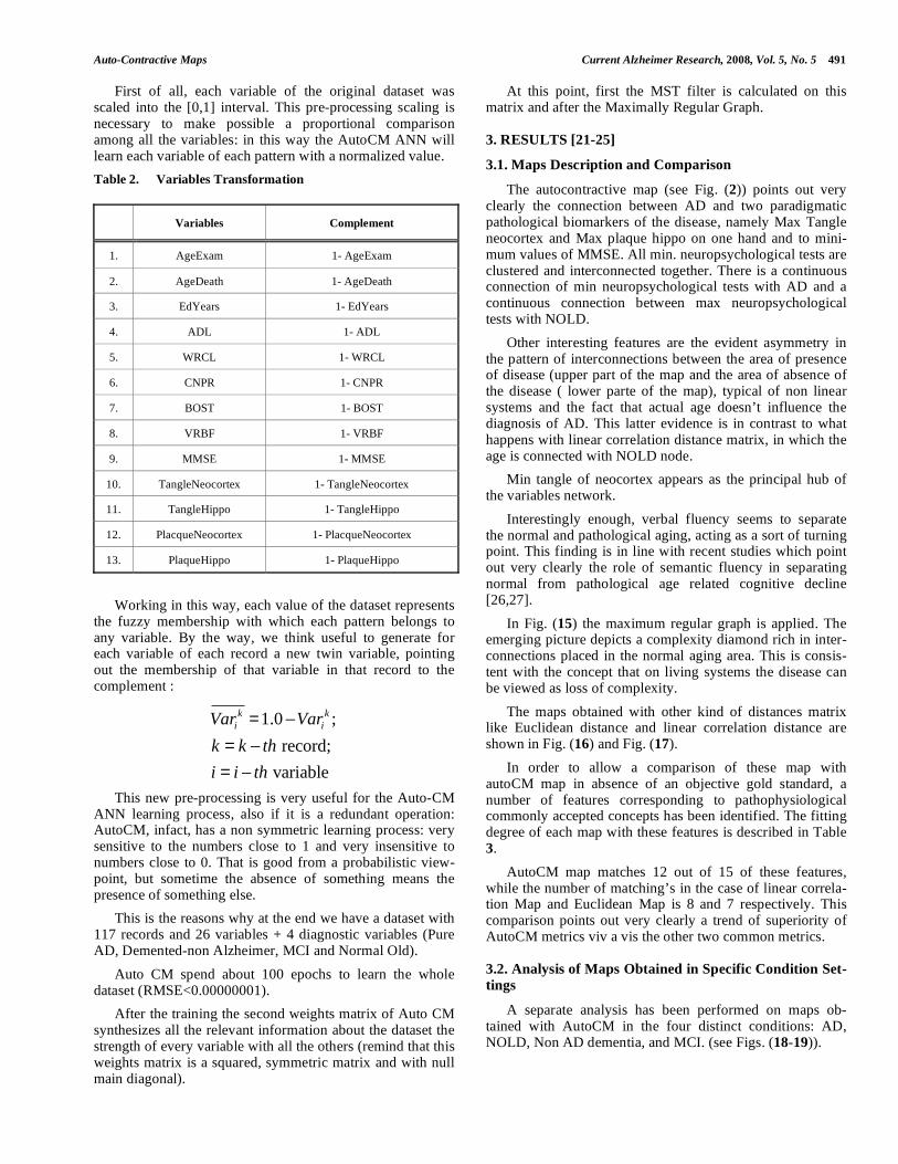
The autocontractive map (see Fig. (2)) points out very clearly the connection between AD and two paradigmatic pathological biomarkers of the disease, namely Max Tangle neocortex and Max plaque hippo on one hand and to mini-mum values of MMSE. All min. neuropsychological tests are clustered and interconnected together. There is a continuous connection of min neuropsychological tests with AD and a continuous connection between max neuropsychological tests with NOLD.

Other interesting features are the evident asymmetry in the pattern of interconnections between the area of presence of disease (upper part of the map and the area of absence of the disease ( lower parte of the map), typical of non linear systems and the fact that actual age doesn’t influence the diagnosis of AD. This latter evidence is in contrast to what happens with linear correlation distance matrix, in which the age is connected with NOLD node.

Min tangle of neocortex appears as the principal hub of the variables network.

Interestingly enough, verbal fluency seems to separate the normal and pathological aging, acting as a sort of turning point. This finding is in line with recent studies which point out very clearly the role of semantic fluency in separating normal from pathological age related cognitive decline [26,27].

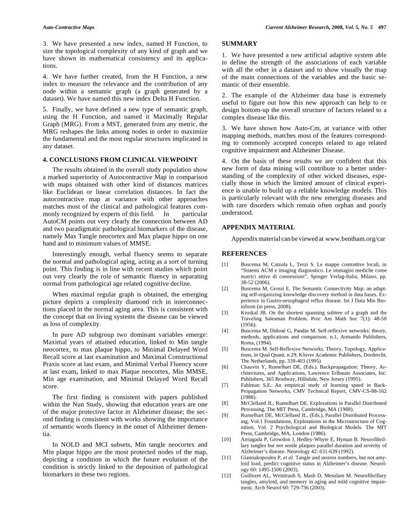
In Fig. (15) the maximum regular graph is applied. The emerging picture depicts a complexity diamond rich in inter-connections placed in the normal aging area. This is consis-tent with the concept that on living systems the disease can be viewed as loss of complexity.

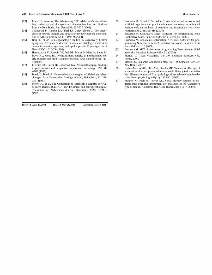
The maps obtained with other kind of distances matrix like Euclidean distance and linear correlation distance are shown in Fig. (16) and Fig. (17).

In order to allow a comparison of these map with autoCM map in absence of an objective gold standard, a number of features corresponding to pathophysiological commonly accepted concepts has been identified. The fitting degree of each map with these features is described in Table 3.

AutoCM map matches 12 out of 15 of these features, while the number of matching’s in the case of linear correla-tion Map and Euclidean Map is 8 and 7 respectively. This comparison points out very clearly a trend of superiority of AutoCM metrics viv a vis the other two common metrics.

3.2. Analysis of Maps Obtained in Specific Condition Set-

tings

A separate analysis has been performed on maps ob-tained with AutoCM in the four distinct conditions: AD, NOLD, Non AD dementia, and MCI. (see Figs. (18-19)).


Fig. (14). Connection between AD Max Tangle neocortex and Max plaque hippo and to minimum values of MMSE.

Fig. (15). AutoCM and Maximally Regular Graph: a complexity diamond rich in inteconnections placed in the normal aging area.

�� ! "#��$��%��&'�()** $

��$��%��&'�� ! "#��$��+,� ��$

��)��-$

��)��.�$

��)��/.�$��)��%0$

��)��12��"3$

��)�40��$

��#5$��+$ ��()** $

��)�60�-$

��)�%��&'�()** $

��)�� ! "#��$

��)��()** $

��)�%��&'�� ! "#��$

��)��+$

��)��#5$

�4��0��$

��.�$

��%0$��/.�$

��60�-$

�� 1$

��-$

�� +,��7$

��12��"3$

��+,� ��$

��)��-$

��%��&'�� ! "#��$ ��$

�� ! "#��$��%��&'�()** $

��)��.�$

��)��/.�$��)��%0$

��)��12��"3$

��)�40��$

��#5$��+$ ��)�60�-$

��()** $

��12��"3$

��)�%��&'�()** $

��)�%��&'�� ! "#��$

��)�� ! "#��$

��)��()** $

��)��+$

��)��#5$

��%0$

�4��0��$

��.�$ ��60�-$

�� 1$

��/.�$

��-$

�� +,��7$


Fig. (16). Map based on Euclidean distance matrix

Fig. (17). Map based on linear correlation distance matrix

��

��

��

��

��

��

��

��

��!"��#�

�� $%��

��&��

�'��(�

��)�

��'��(�

��

��

��

��

��

��

��!"��#�

��

� �$%� ��

� ��

��)�

��$�

��&��

�� $�

�� !�

��/.�$

��12��"3$��%0$ ��.�$

��-$

�� +,��7$

�4��0��$

��60�-$

�� 1$

��)��+$

��)��#5$

��)��()** $

��)�� ! "#��$

��)�%��&'�� ! "#��$

��)�%��&'�()** $

��+,� ��$

��)��-$

��)��.�$

��)�40��$��)�60�-$

��)��%0$ ��)��/.�$

��)��12��"3$

��%��&'�()** $

��$

�� ! "#��$

��%��&'�� ! "#��

��()** $

��+$��#5$


Table 3. Comparison of Three Mapping Methods According to 14 Pathophysiological Accepted Concepts

Distances matrix Feature

Linear correlation Euclidean AutoCM

Significant No. of degrees of separation between NOLD and MCI yes (4) no (2) yes (4)

Significant No. of degrees of separationbetween NOLD and AD yes (9) no (6) yes (9)

Continuous connection pathologic markers presence yes yes no

Continuous connection pathologic markers absence yes yes yes

AD linked with max tangles neocortex yes no yes

NOLD linked with min tangles neocortex no no no

AD Linked with Min neuropsychol test Yes (Min MMSE) yes (min MMSE) yes (min MMSE)

NOLD linked to max neuropsychol test No (max ADL) yes (maxWRCL) yes ( max WRCL)

Continuous connection neuropsychol test min with AD yes yes yes

Continuous connection neuropsychol test max with NOLD yes yes yes

Principal hub (tangle neocortex?) NO (max, min MMSE) No (MMSE, max VRBF) yes

Max education years linked to min tangles neocortex/and or NOLD No (Max CNPR) No (Min plaques neocortex) Yes

(Min Tangle neocortex)

Min education years linked to max tangles/and or AD No (Min CNPR) No (max plaque neocortex) No (Min VRBF)

Min VRBF as turning point between normal and pathological aging No yes yes

Asimmetry of interconnections in AD vs NOLD area No No yes

Total score 8 7 12

Fig. (18). Pure Alzheimer Disease map.

'��(

*+,-

��

*+,.

*+,/

*+.0

��&��

��

*+,.

��

��*+,/

*+,.

*+,.

��!1��#

�� *+,.

*+,/ *+,.

*+,.

*+,-

��$

*+,2

��) ��

��

��

��

��)

��&��

*+,,

��'��(*+,/

*+,.

��

*+,.

*+,.*+,.

*+,,

*+,3

��

��

��

*+,4

��!"��#

��

��

*+,0

*+,2��$


Fig. (19). Non Alzheimer dementia map.

Pure Alzheimer Disease (Fig. (18))

There are two dominant variables: Max education years, linked to Min tangle neocortex, to max plaque hippo (abso-lutely consistent with the overall map), to Min WRCL and Max CNPR, and Min VRBF, linked to max Claque neocor-tex, Min MMSE, Min age examination, and Min WRCL.

The first finding is consistent with papers published within the Nun Study, showing that education years are one of the major protective factor in Alzheimer disease; the sec-ond finding is consistent with works showing the importance of semantic words fluency in the onset of Alzheimer demen-tia.

Minimum education year is a marginal variable, as max tangles in Hippocampus.

Demented Non AD (see Fig.(19))

At variance with AD map, max education years are re-lated to max plaque neocortex, and is not influencing directly the tangles distribution in neocortex. The two hubs are Min tangle neocortex and MIn ADL. Max tangles in hippocam-pus are related to aging effect.

MCI (Fig. (20))

Max age at death is the turning point between normal aging and degenerative disease.

Min tangle neocortex and Min plaque hippo are the most protected nodes of the map, depicting a condition in which the future evolution of the condition is strictly linked to the deposition of pathological biomarkers in these two regions.

NOLD (Fig. (21))

Also in this condition, like MCI, Min tangle neocortex and Min plaque hippo are the most protected nodes of the map, depicting a condition in which the future evolution of the condition is strictly linked to the deposition of pathologi-cal biomarkers in these two regions.

Min semantic verbal fluency is the principal hub of the system, coordinating the biomarkers features on one hand and the maintenance of minimum values of other neuropsy-chological tests.

3. CONCLUSIONS FROM MATHEMATICAL VIEW-

POINT

In this paper we have presented new theoretical hypothe-ses, new mathematical algorithms and new criteria to meas-ure the complexity of the networks:

1. We have presented the math, the topology and the algo-rithm of a new ANN, named Auto Contractive Map (AutoCM). The AutoCM system reshapes the distances among variables or records of any dataset, considering their global vectorial similarities and consequently defining the specific warped space in which variables or records can work.

2. We have shown as a known filter as the MST can be used to cluster a distance matrix, generated from a dataset, in a very useful way.

��

*+,/

��

��

*+,2

��

*+,2 �� *+.-

��&��

��

��!"��#

*+,.*+,.

*+,.*+,/

*+,,

��'��(

*+,4

*+,.

��$

��

��

*+,.

*+,,

*+,,

*+,-

*+,0

��!"��#

��

*+,.

*+,0

��)

��

��

��

��$

*+,2

*+,2

��

��%��&'�� ! "#��

*+.2

�� ! "#��

*+,.

*+,.��

��

��

'��(

*+,5

*+,5

��&��


Fig. (20). MCI map.

Fig. (21). NOLD map.

��*+,. ��*+,.

*+,.

��!"��#

*+,2 *+,.

*+,2

��

'��(

*+,-

��

��

��*+,- � ��6�

*+,,*+,4

*+,,

��

*+,/

*+,.��

��'��(

*+,/*+,3

��

*+,4

��

*+,4

��*+..

��!"��#

�� &�7

*+.3

��

*+2/*+.. ��

��)

*+,0

��$

*+.5

*+23

��

��

*+,2 ��$��)

��&��

*+,2

��

��

��

��

��

��$

*+./

*+,/

��!"��#��*+.-

*+.3

��*+.0 ��

*+,-��'��(

*+,.

*+,/*+5.

��&��

*+,/ *+//

��

��

�� *+,, ��

*+,,

*+,,*+,,

*+,,

*+,,

�� !"

��

'��*+,0

��

��*+,,

��)

*+,,

��$

*+,2

*+,.

*+.,

*+24


3. We have presented a new index, named H Function, to size the topological complexity of any kind of graph and we have shown its mathematical consistency and its applica-tions.

4. We have further created, from the H Function, a new index to measure the relevance and the contribution of any node within a semantic graph (a graph generated by a dataset). We have named this new index Delta H Function.

5. Finally, we have defined a new type of semantic graph, using the H Function, and named it Maximally Regular Graph (MRG). From a MST, generated from any metric, the MRG reshapes the links among nodes in order to maximize the fundamental and the most regular structures implicated in any dataset.

4. CONCLUSIONS FROM CLINICAL VIEWPOINT

The results obtained in the overall study population show a marked superiority of Autocontractive Map in comparison with maps obtained with other kind of distances matrices like Euclidean or linear correlation distances. In fact the autocontractive map at variance with other approaches matches most of the clinical and pathological features com-monly recognized by experts of this field. In particular AutoCM points out very clearly the connection between AD and two paradigmatic pathological biomarkers of the disease, namely Max Tangle neocortex and Max plaque hippo on one hand and to minimum values of MMSE.

Interestingly enough, verbal fluency seems to separate the normal and pathological aging, acting as a sort of turning point. This finding is in line with recent studies which point out very clearly the role of semantic fluency in separating normal from pathological age related cognitive decline.

When maximal regular graph is obtained, the emerging picture depicts a complexity diamond rich in interconnec-tions placed in the normal aging area. This is consistent with the concept that on living systems the disease can be viewed as loss of complexity.

In pure AD subgroup two dominant variables emerge: Maximal years of attained education, linked to Min tangle neocortex, to max plaque hippo, to Minimal Delayed Word Recall score at last examination and Maximal Constructional Praxis score at last exam, and Minimal Verbal Fluency score at last exam, linked to max Plaque neocortex, Min MMSE, Min age examination, and Minimal Delayed Word Recall score.

The first finding is consistent with papers published within the Nun Study, showing that education years are one of the major protective factor in Alzheimer disease; the sec-ond finding is consistent with works showing the importance of semantic words fluency in the onset of Alzheimer demen-tia.

In NOLD and MCI subsets, Min tangle neocortex and Min plaque hippo are the most protected nodes of the map, depicting a condition in which the future evolution of the condition is strictly linked to the deposition of pathological biomarkers in these two regions.

SUMMARY

1. We have presented a new artificial adaptive system able to define the strength of the associations of each variable with all the other in a dataset and to show visually the map of the main connections of the variables and the basic se-mantic of their ensemble.

2. The example of the Alzheimer data base is extremely useful to figure out how this new approach can help to re design bottom-up the overall structure of factors related to a complex disease like this.

3. We have shown how Auto-Cm, at variance with other mapping methods, matches most of the features correspond-ing to commonly accepted concepts related to age related cognitive impairment and Alzheimer Disease.

4. On the basis of these results we are confident that this new form of data mining will contribute to a better under-standing of the complexity of other wicked diseases, espe-cially those in which the limited amount of clinical experi-ence is unable to build up a reliable knowledge models. This is particularly relevant with the new emerging diseases and with rare disorders which remain often orphan and poorly understood.

APPENDIX MATERIAL

Appendix material can be viewed at www.bentham.org/car

REFERENCES

[1] Buscema M, Catzola L, Terzi S. Le mappe contrattive locali, in “Sistemi ACM e imaging diagnostico. Le immagini mediche come

matrici attive di connessioni”, Spinger Verlag-Italia, Milano, pp. 38-52 (2006).

[2] Buscema M, Grossi E. The Semantic Connectivity Map: an adapt-ing self-organizing knowledge discovery method in data bases. Ex-

perience in Gastro-oesophageal reflux disease. Int J Data Min Bio-inform (in press, 2008).

[3] Kruskal JB. On the shortest spanning subtree of a graph and the Traveling Salesman Problem. Proc Am Math Soc 7(1): 48-50

(1956). [4] Buscema M, Didoné G, Pandin M. Self-reflexive networks: theory,

methods, applications and comparison. n.1, Armando Publishers, Roma, (1994).

[5] Buscema M. Self-Reflexive Networks. Theory, Topology, Applica-tions, in Qual Quant, n.29, Kluver Academic Publishers, Dordrecht,

The Netherlands, pp. 339-403 (1995) [6] Chauvin Y, Rumelhart DE, (Eds.). Backpropagation: Theory, Ar-

chitectures, and Applications, Lawrence Erlbaum Associates, Inc. Publishers, 365 Brodway, Hillsdale, New Jersey (1995).

[7] Fahlman S.E. An empirical study of learning speed in Back-Propagation Networks, CMV Technical Report, CMV-CS-88-162

(1988). [8] McClelland JL, Rumelhart DE. Explorations in Parallel Distributed

Processing, The MIT Press, Cambridge, MA (1988). [9] Rumelhart DE, McClelland JL, (Eds.), Parallel Distributed Process-

ing, Vol.1 Foundations, Explorations in the Microstructure of Cog-nition, Vol. 2 Psychological and Biological Models. The MIT

Press, Cambridge, MA, London (1986). [10] Arriagada P, Growdon J, Hedley-Whyte E, Hyman B. Neurofibril-

lary tangles but not senile plaques parallel duration and severity of Alzheimer’s disease. Neurology 42: 631-639 (1992).

[11] Giannakopoulos P, et al. Tangle and neuron numbers, but not amy-loid load, predict cognitive status in Alzheimer’s disease. Neurol-

ogy 60: 1495-1500 (2003). [12] Guillozet AL, Weintraub S, Mash D, Mesulam M. Neurofibrillary

tangles, amyloid, and memory in aging and mild cognitive impair-ment. Arch Neurol 60: 729-736 (2003).


[13] Riley KP, Snowdon DA, Markesbery WR. Alzheimer’s neurofibril-

lary pathology and the spectrum of cognitive function: findings from the Nun Study. Ann Neurol 51: 567-577 (2002).

[14] Tiraboschi P, Hansen LA, Thal LJ, Corey-Bloom J. The impor-tance of neuritic plaques and tangles to the development and evolu-

tion of AD. Neurology 62(11): 1984-9 (2004). [15] Berg L, et al. Clinicopathologic studies in cognitively healthy

aging and Alzheimer's disease: relation of histologic markers to dementia severity, age, sex, and apolipoprotein E genotype. Arch

Neurol 55(3): 326-35 (1998). [16] Haroutunian V, Purohit DP, Perl DP, Marin D, Khan K, Lantz M,

Davis KL, Mohs RC. Neurofibrillary tangles in nondemented eld-erly subjects and mild Alzheimer disease. Arch Neurol 56(6): 713-

8 (1999). [17] Petersen RC, Parisi JE, Johonson KA. Neuropathological findings

in patients with mild cognitive impairment. Neurology 1997; 48: A102 (1997).

[18] Braak H, Braak E. Neuropathological staging of Alzheimer related changes. Acta Neuropathol, Springer-Verlag, Heidelberg, 82: 239-

259 (1991). [19] Morris JC, et al. The Consortium to Establish a Registry for Alz-

heimer's Disease (CERAD). Part I. Clinical and neuropsychological assessment of Alzheimer's disease. Neurology 39(9): 1159-65

(1989).

[20] Buscema M, Grossi E, Snowdon D. Artificial neural networks and

artificial organisms can predict Alzheimer pathology in individual patients only on the basis of cognitive and functional status. Neu-

roinformatics 2(4): 399-416 (2004). [21] Buscema M. Contractive Maps. Software for programming Auto

Contractive Maps, Semeion Software #15, ver 2.0 (2007). [22] Buscema M. Constraints Satisfaction Networks. Software for pro-

gramming Non Linear Auto-Associative Networks, Semeion Soft-ware #14, ver 10.0 (2008).

[23] Buscema M. MST. Software for programming Trees from artificial networks, Semeion Software #38 v 5.1 (2008).

[24] Massini G. Trees Visualizer, Ver 3.0, Semeion Software #40, Rome, 2007.

[25] Massini G. Semantic Connection Map, Ver 1.0, Semeion Software #45, Rome, 2007.

[26] Forbes-McKay KE, Ellis AW, Shanks MF, Venneri A. The age of acquisition of words produced in a semantic fluency task can relia-

bly differentiate normal from pathological age related cognitive de-cline. Neuropsychologia 43(11): 1625-32. (2005).

[27] Murphy KJ, Rich JB, Troyer AK. Verbal fluency patterns in am-nestic mild cognitive impairment are characteristic of Alzheimer's

type dementia. Alzheimer Dis Assoc Disord 21(1): 65-7 (2007).

Received: April 16, 2008 Revised: May 28, 2008 Accepted: May 30, 2008

Auto-Contractive Maps Current Alzheimer Research, 2008, Vol. 5, No. 5 i

APPENDIX

AutoCM, MST, the H Function and the MRG: An

Example

Let us now consider a toy dataset to test how the previous formalism works in practice and what kind of insight it yields for a given problem. In what follows, we will guide the reader along a thorough illustration of the techniques introduced so far. We will work on the Gang dataset, a small, very well known and widely used dataset, made of 27 re-cords and 5 variables, and clearly modeled on the West Side

Story musical:

The structure of the dataset is the following:

• Gang = {Jets, Sharks};

• Age = {20’s, 30’s, 40’s};

• Education = {Junior School, High School, College};

• Status = {Married, Single, Divorced};

• Profession = {Pusher, Bookie, Burglar}.

Table 4. Gang Dataset

Name Gang Age Education Status Profession

ART Jet 40 JH Single Pusher

AL Jet 30 JH Married Burglar

SAM Jet 20 COL Single Bookie

CLYDE Jet 40 JH Single Bookie

MIKE Jet 30 JH Single Bookie

JIM Jet 20 JH Divorced Burglar

GREG Jet 20 HS Married Pusher

JOHN Jet 20 JH Married Burglar

DOUG Jet 30 HS Single Bookie

LANCE Jet 20 JH Married Burglar

GEORGE Jet 20 JH Divorced Burglar

PETE Jet 20 HS Single Bookie

FRED Jet 20 HS Single Pusher

GENE Jet 20 COL Single Pusher

RALPH Jet 30 JH Single Pusher

PHIL Sharks 30 COL Married Pusher

IKE Sharks 30 JH Single Bookie

NICK Sharks 30 HS Single Pusher

DON Sharks 30 COL Married Burglar

NED Sharks 30 COL Married Bookie

KARL Sharks 40 HS Married Bookie

KEN Sharks 20 HS Single Burglar

EARL Sharks 40 HS Married Burglar

RICK Sharks 30 HS Divorced Burglar

OL Sharks 30 COL Married Pusher

NEAL Sharks 30 HS Single Bookie

DAVE Sharks 30 HS Divorced Pusher

ii Current Alzheimer Research, 2008, Vol. 5, No. 5 Buscema et al.

Table 5. Binary Gang Dataset

Nome Jet Sharks 20 30 40 JH COL HS Single Married Divorced Pusher Bookie Burglar

ART 1 0 0 0 1 1 0 0 1 0 0 1 0 0

AL 1 0 0 1 0 1 0 0 0 1 0 0 0 1

SAM 1 0 1 0 0 0 1 0 1 0 0 0 1 0

CLYDE 1 0 0 0 1 1 0 0 1 0 0 0 1 0

MIKE 1 0 0 1 0 1 0 0 1 0 0 0 1 0

JIM 1 0 1 0 0 1 0 0 0 0 1 0 0 1

GREG 1 0 1 0 0 0 0 1 0 1 0 1 0 0

JOHN 1 0 1 0 0 1 0 0 0 1 0 0 0 1

DOUG 1 0 0 1 0 0 0 1 1 0 0 0 1 0

LANCE 1 0 1 0 0 1 0 0 0 1 0 0 0 1

GEORGE 1 0 1 0 0 1 0 0 0 0 1 0 0 1

PETE 1 0 1 0 0 0 0 1 1 0 0 0 1 0

FRED 1 0 1 0 0 0 0 1 1 0 0 1 0 0

GENE 1 0 1 0 0 0 1 0 1 0 0 1 0 0

RALPH 1 0 0 1 0 1 0 0 1 0 0 1 0 0

PHIL 0 1 0 1 0 0 1 0 0 1 0 1 0 0

IKE 0 1 0 1 0 1 0 0 1 0 0 0 1 0

NICK 0 1 0 1 0 0 0 1 1 0 0 1 0 0

DON 0 1 0 1 0 0 1 0 0 1 0 0 0 1

NED 0 1 0 1 0 0 1 0 0 1 0 0 1 0

KARL 0 1 0 0 1 0 0 1 0 1 0 0 1 0

KEN 0 1 1 0 0 0 0 1 1 0 0 0 0 1

EARL 0 1 0 0 1 0 0 1 0 1 0 0 0 1

RICK 0 1 0 1 0 0 0 1 0 0 1 0 0 1

OL 0 1 0 1 0 0 1 0 0 1 0 1 0 0

NEAL 0 1 0 1 0 0 0 1 1 0 0 0 1 0

DAVE 0 1 0 1 0 0 0 1 0 0 1 1 0 0

Table 6 . Gang Dataset Transposed

Name Art Al Sam Clyde Mike Jim Greg John Doug Lance George Pete Fred Gene Ralph Phil Ike Nick Don Ned Karl Ken Earl Rick Ol Neal Dave

Jet 1 1 1 1 1 1 1 1 1 1 1 1 1 1 1 0 0 0 0 0 0 0 0 0 0 0 0

Sharks 0 0 0 0 0 0 0 0 0 0 0 0 0 0 0 1 1 1 1 1 1 1 1 1 1 1 1

20 0 0 1 0 0 1 1 1 0 1 1 1 1 1 0 0 0 0 0 0 0 1 0 0 0 0 0

30 0 1 0 0 1 0 0 0 1 0 0 0 0 0 1 1 1 1 1 1 0 0 0 1 1 1 1

Auto-Contractive Maps Current Alzheimer Research, 2008, Vol. 5, No. 5 iii

(Table 6) contd….

Name Art Al Sam Clyde Mike Jim Greg John Doug Lance George Pete Fred Gene Ralph Phil Ike Nick Don Ned Karl Ken Earl Rick Ol Neal Dave

40 1 0 0 1 0 0 0 0 0 0 0 0 0 0 0 0 0 0 0 0 1 0 1 0 0 0 0

JH 1 1 0 1 1 1 0 1 0 1 1 0 0 0 1 0 1 0 0 0 0 0 0 0 0 0 0

COL 0 0 1 0 0 0 0 0 0 0 0 0 0 1 0 1 0 0 1 1 0 0 0 0 1 0 0

HS 0 0 0 0 0 0 1 0 1 0 0 1 1 0 0 0 0 1 0 0 1 1 1 1 0 1 1

Single 1 0 1 1 1 0 0 0 1 0 0 1 1 1 1 0 1 1 0 0 0 1 0 0 0 1 0

Married 0 1 0 0 0 0 1 1 0 1 0 0 0 0 0 1 0 0 1 1 1 0 1 0 1 0 0

Divorced 0 0 0 0 0 1 0 0 0 0 1 0 0 0 0 0 0 0 0 0 0 0 0 1 0 0 1

Pusher 1 0 0 0 0 0 1 0 0 0 0 0 1 1 1 1 0 1 0 0 0 0 0 0 1 0 1

Bookie 0 0 1 1 1 0 0 0 1 0 0 1 0 0 0 0 1 0 0 1 1 0 0 0 0 1 0

Burglar 0 1 0 0 0 1 0 1 0 1 1 0 0 0 0 0 0 0 1 0 0 1 1 1 0 0 0

First of all, it is necessary to transform each string variable into a Boolean one (see Table 5).

The new dataset is now made of 14 binary variables, most of which orthogonal to each other. As we want to use a AutoCM ANN to process the records, we must, as remarked above, transpose this matrix (see Table 6).

The dataset is then submitted to the AutoCM ANN for the learning session. The set is structured such that the vari-ables are the hyper-points and the records are the hyper-points coordinates. After about 30 epochs, the AutoCM, with a contractive factor of 6.19615221, is completely trained (RMSE=0.00000000) and the weights matrix reads as in Table 7.

Applying equation (12), we transform the weights matrix into a distance matrix (Table 8). We can therefore now com-pute the MST of the dataset, that turns out to be as in Fig. (22).

What does the MST tell us? It provides a ready-to-access spatialization of the complex pattern of associations among the variables that characterize each one of the Gang mem-bers, as well as their belonging to a specific Gang. In par-ticular, notice how the MST perfectly separates the two Gangs into sub-trees whose boundaries are marked, respec-tively, by Ike and Mike. Close-by subjects in the networks correspond to subjects that basically present close-by per-sonal characteristics; moreover, the tree structure clearly points out how specific subsets of subjects constitute sub-families of common traits within the large Gang family. Nothing like this neat, hands-on representation of variables association can be obtained by means of the today classic techniques.

Let us consider again the Gang dataset (Table 4) to com-pute its MRG (Fig. 11).

In this example, the H Function reaches its peak when the seventh of the connections skipped during the MST genera-tion is added back. So the MRG needs seven extra connec-tions to be added to the MST and, consequently, the H Func-tion value is almost 50% higher with respect to its value at the original MST (H(0)=10.99 vs. H(7)=15.38). It is then not

surprising that the structure of the two graphs turns out very different (Figs. 24-25).

The MRG carries a richer amount of information than the MST. The boundary between the two Gangs, i.e. between Jets and Sharks members, is now represented no longer by a couple of subjects, but rather by a cycle of four subjects: Neal and Ken are Sharks, while Doug and Mike are Jets. So, looking at the MRG, the edges between Jets and Sharks seem apparently to be fuzzy and negotiable, and in particular less clear-cut than in the MST case. But this appearance is very misleading. In fact, the four subjects lying on the border are all outliers in their respective Gangs: by placing them all on the border, this feature becomes much clearer and pro-vides a better insight of what makes a ‘typical’ Jet or Shark. Furthermore, Al, a member of the Jets Gang, is placed at the top of an autonomous circuit of links among four Jets mem-bers, as he is the head of a new virtual gang hidden into the Jets Gang. Looking at the MRG, moreover, we also receive more information about the internal structure of the two Gangs: because of the bigger number of cycles, the Jets Gang reveals itself as more complex and articulated that the Sharks Gang. Finally, the cycle including Don, Ol, and Phil represents a prototype of the Sharks member, whose features are very different from Jets subjects. In the same way, Jets show two different prototypes; the first is represented by the cycle including Gene, Sam, Fred and Pete; the second by the cycle including John, George, Lance and Jim.

According to the MRG, the structural features of each prototype may be stated as follows:

Prototype of Gang hybridization:

30 'Jets JuniorSchool

Single BookieSharks HighSchool

+ + + +

Prototype of Sharks member:

30'+ College + Married +Pusher

Burglar.

iv Current Alzheimer Research, 2008, Vol. 5, No. 5 Buscema et al.

Table 7. AutoCM Weights Matrix

Art Al Sam Clyde Mike Jim Greg John Doug Lance George Pete Fred Gene Ralph Phil Ike Nick Don Ned Karl Ken Earl Rick Ol Neal Dave

0.000 102.834 119.919 165.020 148.799 105.244 111.426 103.889 117.112 103.889 105.244 114.937 154.444 156.809 167.015 31.696 108.600 102.582 1.000 1.000 11.014 46.859 13.070 1.000 31.696 42.051 30.909

102.834 0.000 52.305 103.376 157.458 147.536 122.170 168.077 135.954 168.077 147.536 51.757 51.388 51.945 156.251 113.351 104.773 42.032 150.804 113.245 33.006 24.152 88.161 112.030 113.351 42.873 47.696

119.919 52.305 0.000 153.459 148.718 105.003 104.284 103.247 147.552 103.247 105.003 166.467 148.991 169.141 114.741 17.260 92.509 40.033 20.263 77.737 27.947 104.274 1.000 1.000 17.260 92.003 1.000

165.020 103.376 153.459 0.000 165.808 105.799 50.718 104.438 147.952 104.438 105.799 150.009 117.157 122.032 148.535 1.000 143.323 41.177 1.000 26.595 62.466 45.402 11.290 1.000 1.000 92.771 1.000

148.799 157.458 148.718 165.808 0.000 103.037 49.933 101.711 170.651 101.711 103.037 145.375 112.342 117.016 171.263 47.817 166.984 116.334 50.503 105.685 23.671 39.402 1.000 49.821 47.817 146.379 48.501

105.244 147.536 105.003 105.799 103.037 0.000 106.052 166.100 54.289 166.100 173.095 102.374 101.484 103.642 102.161 1.000 31.094 1.000 30.222 1.000 1.000 88.422 29.959 62.254 1.000 1.000 10.990

111.426 122.170 104.284 50.718 49.933 106.052 0.000 153.875 124.990 153.875 106.052 152.993 168.789 144.173 101.022 96.924 1.000 83.742 30.533 36.126 114.075 89.111 110.912 40.009 96.924 32.772 99.136

103.889 168.077 103.247 104.438 101.711 166.100 153.875 0.000 52.905 175.974 166.100 100.661 99.786 101.908 100.847 37.300 30.762 1.000 96.504 38.949 41.485 81.929 97.605 27.089 37.300 1.000 1.000

117.112 135.954 147.552 147.952 170.651 54.289 124.990 52.905 0.000 52.905 54.289 168.134 155.766 118.147 160.011 44.659 139.563 150.844 47.167 98.804 88.449 99.168 36.207 117.377 44.659 165.251 114.304

103.889 168.077 103.247 104.438 101.711 166.100 153.875 175.974 52.905 0.000 166.100 100.661 99.786 101.908 100.847 37.300 30.762 1.000 96.504 38.949 41.485 81.929 97.605 27.089 37.300 1.000 1.000

105.244 147.536 105.003 105.799 103.037 173.095 106.052 166.100 54.289 166.100 0.000 102.374 101.484 103.642 102.161 1.000 31.094 1.000 30.222 1.000 1.000 88.422 29.959 62.254 1.000 1.000 10.990

114.937 51.757 166.467 150.009 145.375 102.374 152.993 100.661 168.134 100.661 102.374 0.000 169.389 148.663 109.974 1.000 85.270 103.911 1.000 25.279 101.294 146.151 41.011 39.203 1.000 140.722 36.636

154.444 51.388 148.991 117.157 112.342 101.484 168.789 99.786 155.766 99.786 101.484 169.389 0.000 167.879 147.391 27.467 36.296 144.155 1.000 1.000 37.382 146.992 40.644 38.852 27.467 106.633 100.301

156.809 51.945 169.141 122.032 117.016 103.642 144.173 101.908 118.147 101.908 103.642 148.663 167.879 0.000 149.649 75.216 41.826 98.437 18.665 16.130 1.000 105.880 1.000 1.000 75.216 42.204 26.616

167.015 156.251 114.741 148.535 171.263 102.161 101.022 100.847 160.011 100.847 102.161 109.974 147.391 149.649 0.000 104.638 152.591 146.988 48.224 43.796 1.000 40.438 1.000 47.572 104.638 115.436 104.421

31.696 113.351 17.260 1.000 47.817 1.000 96.924 37.300 44.659 37.300 1.000 1.000 27.467 75.216 104.638 0.000 108.975 144.391 165.747 165.721 106.454 38.362 101.821 109.503 175.413 104.604 151.985

108.600 104.773 92.509 143.323 166.984 31.094 1.000 30.762 139.563 30.762 31.094 85.270 36.296 41.826 152.591 108.975 0.000 154.280 109.004 145.738 95.366 124.229 37.850 107.324 108.975 167.224 107.455

102.582 42.032 40.033 41.177 116.334 1.000 83.742 1.000 150.844 1.000 1.000 103.911 144.155 98.437 146.988 144.391 154.280 0.000 103.993 101.947 95.758 152.929 99.624 148.304 144.391 169.391 166.046

1.000 150.804 20.263 1.000 50.503 30.222 30.533 96.504 47.167 96.504 30.222 1.000 1.000 18.665 48.224 165.747 109.004 103.993 0.000 165.637 99.470 103.860 145.643 153.536 165.747 104.632 109.665

1.000 113.245 77.737 26.595 105.685 1.000 36.126 38.949 98.804 38.949 1.000 25.279 1.000 16.130 43.796 165.721 145.738 101.947 165.637 0.000 152.280 37.628 102.677 107.377 165.721 142.295 107.507

11.014 33.006 27.947 62.466 23.671 1.000 114.075 41.485 88.449 41.485 1.000 101.294 37.382 1.000 1.000 106.454 95.366 95.758 99.470 152.280 0.000 105.496 166.131 104.257 106.454 139.097 102.993

46.859 24.152 104.274 45.402 39.402 88.422 89.111 81.929 99.168 81.929 88.422 146.151 146.992 105.880 40.438 38.362 124.229 152.929 103.860 37.628 105.496 0.000 152.021 149.552 38.362 153.340 101.379

13.070 88.161 1.000 11.290 1.000 29.959 110.912 97.605 36.207 97.605 29.959 41.011 40.644 1.000 1.000 101.821 37.850 99.624 145.643 102.677 166.131 152.021 0.000 153.007 101.821 101.153 107.151

1.000 112.030 1.000 1.000 49.821 62.254 40.009 27.089 117.377 27.089 62.254 39.203 38.852 1.000 47.572 109.503 107.324 148.304 153.536 107.377 104.257 149.552 153.007 0.000 109.503 149.444 164.739

31.696 113.351 17.260 1.000 47.817 1.000 96.924 37.300 44.659 37.300 1.000 1.000 27.467 75.216 104.638 175.413 108.975 144.391 165.747 165.721 106.454 38.362 101.821 109.503 0.000 104.604 151.985

42.051 42.873 92.003 92.771 146.379 1.000 32.772 1.000 165.251 1.000 1.000 140.722 106.633 42.204 115.436 104.604 167.224 169.391 104.632 142.295 139.097 153.340 101.153 149.444 104.604 0.000 148.500

30.909 47.696 1.000 1.000 48.501 10.990 99.136 1.000 114.304 1.000 10.990 36.636 100.301 26.616 104.421 151.985 107.455 166.046 109.665 107.507 102.993 101.379 107.151 164.739 151.985 148.500 0.000

Table 8. AutoCM Distance Matrix


0.000 0.569 0.664 0.914 0.824 0.583 0.617 0.575 0.649 0.575 0.583 0.637 0.855 0.868 0.925 0.176 0.601 0.568 0.006 0.006 0.061 0.259 0.072 0.006 0.176 0.233 0.171

0.569 0.000 0.290 0.572 0.872 0.817 0.677 0.931 0.753 0.931 0.817 0.287 0.285 0.288 0.865 0.628 0.580 0.233 0.835 0.627 0.183 0.134 0.488 0.620 0.628 0.237 0.264

0.664 0.290 0.000 0.850 0.824 0.581 0.578 0.572 0.817 0.572 0.581 0.922 0.825 0.937 0.635 0.096 0.512 0.222 0.112 0.430 0.155 0.577 0.006 0.006 0.096 0.509 0.006

0.914 0.572 0.850 0.000 0.918 0.586 0.281 0.578 0.819 0.578 0.586 0.831 0.649 0.676 0.823 0.006 0.794 0.228 0.006 0.147 0.346 0.251 0.063 0.006 0.006 0.514 0.006

0.824 0.872 0.824 0.918 0.000 0.571 0.277 0.563 0.945 0.563 0.571 0.805 0.622 0.648 0.948 0.265 0.925 0.644 0.280 0.585 0.131 0.218 0.006 0.276 0.265 0.811 0.269

Auto-Contractive Maps Current Alzheimer Research, 2008, Vol. 5, No. 5 v

(Table 8) contd…


0.583 0.817 0.581 0.586 0.571 0.000 0.587 0.920 0.301 0.920 0.959 0.567 0.562 0.574 0.566 0.006 0.172 0.006 0.167 0.006 0.006 0.490 0.166 0.345 0.006 0.006 0.061

0.617 0.677 0.578 0.281 0.277 0.587 0.000 0.852 0.692 0.852 0.587 0.847 0.935 0.798 0.559 0.537 0.006 0.464 0.169 0.200 0.632 0.493 0.614 0.222 0.537 0.181 0.549

0.575 0.931 0.572 0.578 0.563 0.920 0.852 0.000 0.293 0.975 0.920 0.557 0.553 0.564 0.558 0.207 0.170 0.006 0.534 0.216 0.230 0.454 0.541 0.150 0.207 0.006 0.006

0.649 0.753 0.817 0.819 0.945 0.301 0.692 0.293 0.000 0.293 0.301 0.931 0.863 0.654 0.886 0.247 0.773 0.835 0.261 0.547 0.490 0.549 0.201 0.650 0.247 0.915 0.633

0.575 0.931 0.572 0.578 0.563 0.920 0.852 0.975 0.293 0.000 0.920 0.557 0.553 0.564 0.558 0.207 0.170 0.006 0.534 0.216 0.230 0.454 0.541 0.150 0.207 0.006 0.006

0.583 0.817 0.581 0.586 0.571 0.959 0.587 0.920 0.301 0.920 0.000 0.567 0.562 0.574 0.566 0.006 0.172 0.006 0.167 0.006 0.006 0.490 0.166 0.345 0.006 0.006 0.061

0.637 0.287 0.922 0.831 0.805 0.567 0.847 0.557 0.931 0.557 0.567 0.000 0.938 0.823 0.609 0.006 0.472 0.575 0.006 0.140 0.561 0.809 0.227 0.217 0.006 0.779 0.203

0.855 0.285 0.825 0.649 0.622 0.562 0.935 0.553 0.863 0.553 0.562 0.938 0.000 0.930 0.816 0.152 0.201 0.798 0.006 0.006 0.207 0.814 0.225 0.215 0.152 0.591 0.555

0.868 0.288 0.937 0.676 0.648 0.574 0.798 0.564 0.654 0.564 0.574 0.823 0.930 0.000 0.829 0.417 0.232 0.545 0.103 0.089 0.006 0.586 0.006 0.006 0.417 0.234 0.147

0.925 0.865 0.635 0.823 0.948 0.566 0.559 0.558 0.886 0.558 0.566 0.609 0.816 0.829 0.000 0.579 0.845 0.814 0.267 0.243 0.006 0.224 0.006 0.263 0.579 0.639 0.578

0.176 0.628 0.096 0.006 0.265 0.006 0.537 0.207 0.247 0.207 0.006 0.006 0.152 0.417 0.579 0.000 0.603 0.800 0.918 0.918 0.590 0.212 0.564 0.606 0.971 0.579 0.842

0.601 0.580 0.512 0.794 0.925 0.172 0.006 0.170 0.773 0.170 0.172 0.472 0.201 0.232 0.845 0.603 0.000 0.854 0.604 0.807 0.528 0.688 0.210 0.594 0.603 0.926 0.595

0.568 0.233 0.222 0.228 0.644 0.006 0.464 0.006 0.835 0.006 0.006 0.575 0.798 0.545 0.814 0.800 0.854 0.000 0.576 0.565 0.530 0.847 0.552 0.821 0.800 0.938 0.920

0.006 0.835 0.112 0.006 0.280 0.167 0.169 0.534 0.261 0.534 0.167 0.006 0.006 0.103 0.267 0.918 0.604 0.576 0.000 0.917 0.551 0.575 0.807 0.850 0.918 0.579 0.607

0.006 0.627 0.430 0.147 0.585 0.006 0.200 0.216 0.547 0.216 0.006 0.140 0.006 0.089 0.243 0.918 0.807 0.565 0.917 0.000 0.843 0.208 0.569 0.595 0.918 0.788 0.595

0.061 0.183 0.155 0.346 0.131 0.006 0.632 0.230 0.490 0.230 0.006 0.561 0.207 0.006 0.006 0.590 0.528 0.530 0.551 0.843 0.000 0.584 0.920 0.577 0.590 0.770 0.570

0.259 0.134 0.577 0.251 0.218 0.490 0.493 0.454 0.549 0.454 0.490 0.809 0.814 0.586 0.224 0.212 0.688 0.847 0.575 0.208 0.584 0.000 0.842 0.828 0.212 0.849 0.561

0.072 0.488 0.006 0.063 0.006 0.166 0.614 0.541 0.201 0.541 0.166 0.227 0.225 0.006 0.006 0.564 0.210 0.552 0.807 0.569 0.920 0.842 0.000 0.847 0.564 0.560 0.593

0.006 0.620 0.006 0.006 0.276 0.345 0.222 0.150 0.650 0.150 0.345 0.217 0.215 0.006 0.263 0.606 0.594 0.821 0.850 0.595 0.577 0.828 0.847 0.000 0.606 0.828 0.912

0.176 0.628 0.096 0.006 0.265 0.006 0.537 0.207 0.247 0.207 0.006 0.006 0.152 0.417 0.579 0.971 0.603 0.800 0.918 0.918 0.590 0.212 0.564 0.606 0.000 0.579 0.842

0.233 0.237 0.509 0.514 0.811 0.006 0.181 0.006 0.915 0.006 0.006 0.779 0.591 0.234 0.639 0.579 0.926 0.938 0.579 0.788 0.770 0.849 0.560 0.828 0.579 0.000 0.822

0.171 0.264 0.006 0.006 0.269 0.061 0.549 0.006 0.633 0.006 0.061 0.203 0.555 0.147 0.578 0.842 0.595 0.920 0.607 0.595 0.570 0.561 0.593 0.912 0.842 0.822 0.000

Fig. (22). The MST of the global network (H0=0.10989).

��

� ��7

��

��

�7�8

8��

��'��7�8

8��

�� 78�

� "��

�78�

��9:

��

:��:

(�� :��

��

��

��

;7�

:��:�

;��

vi Current Alzheimer Research, 2008, Vol. 5, No. 5 Buscema et al.

Fig. (23). Computing the MRG Hubness of the Gang Dataset.

Fig. (24). MST of the Gang dataset.

Fig. (25). MRG of the Gang dataset.

��

��

��

��

��

��

��

�

� �

��

��

��

��

��

��

��

��

��

��

��

��

��

�

��

�

��

��

� �

�

��

��

� � � � � � � � � � � � �

('88��339-)�:3

�;�/0;�$

�</(�$

�<7�$

�-��$ ��-$

��-2��$

�=��$��-$

��7=�$

�7=�$

��/>;$

�%��$

��0��$

�;��$�;0�;$

�.��$

�0�-%($

��0�$

��7�=$

��4�$

�07�=$

��/�$

��0-$

�=�0-$

�/-$

��$

�%(7-$

��

��

��

��

��

��

��

��

��

��

��

��

��

��

��

��

��

��

��

��

��

�8��

��

��7�8��'��

��

��

��7�8�

�8��

��

78��

��9:��78��

��(��:��:�

�:��

�� "��

��

�;��

�;7��

��

� ��:��:��

��7 �

Auto-Contractive Maps Current Alzheimer Research, 2008, Vol. 5, No. 5 vii

First prototype of Jets member:

20 ' .College Bookie

SingleHighSchool Pusher

+ + +

Second prototype of Jets member:

20 ' .Married

JuniorSchool BurglarDivorced

+ + +

Compared to the MST, therefore, the MRG adds all and only those extra features that are really useful in understand-ing the prototypes that are hidden into the database: in other words, it adds the optimal amount of complexity that is nec-essary to read the phenomenon. Dropping any information from the MRG would amount to oversimplifying the repre-sentation; adding more information would amount to mess-ing it up with irrelevant details.

Auto-Contractive Maps: An Artificial Adaptive System for Data Mining. An Application to Alzheimer...

Documents

Transcript of Auto-Contractive Maps: An Artificial Adaptive System for Data Mining. An Application to Alzheimer...