LUND UNIVERSITY

PO Box 117221 00 Lund+46 46-222 00 00

Adaptive Control -- A Way to Deal with Uncertainty

Åström, Karl Johan

1987

Document Version:Publisher's PDF, also known as Version of record

Link to publication

Citation for published version (APA):Åström, K. J. (1987). Adaptive Control -- A Way to Deal with Uncertainty. (Technical Reports TFRT-7345).Department of Automatic Control, Lund Institute of Technology (LTH).

Total number of authors:1

General rightsUnless other specific re-use rights are stated the following general rights apply:Copyright and moral rights for the publications made accessible in the public portal are retained by the authorsand/or other copyright owners and it is a condition of accessing publications that users recognise and abide by thelegal requirements associated with these rights. • Users may download and print one copy of any publication from the public portal for the purpose of private studyor research. • You may not further distribute the material or use it for any profit-making activity or commercial gain • You may freely distribute the URL identifying the publication in the public portal

Read more about Creative commons licenses: https://creativecommons.org/licenses/Take down policyIf you believe that this document breaches copyright please contact us providing details, and we will removeaccess to the work immediately and investigate your claim.

CODEN: LUTT.D2/(TFRT -7 545)lI-zz/(IsB7 )

ADAPTIVE CONTROL

-A way to deal with uncertainty

I(arl Johan Aström

Department of Automatic Control

Lund Institute of Technolory

Febmary 1987

Language

English

S ecu rity class ificat io n

Number of pages

22

Author(s)

Karl Johan Å.ström

Department of Automatic ControlLund Institute of TechnologyP.O. Box 1185-22100 Lund Sweden

ISSN and key title -TSBN

Recipient's notes

inform,ationS up pleme nt ary b iblio gra phical

Classifrcation systern index terms (if

Key w'ords

Abstræt

This paper was presented at the DFVLR International Seminar "IJncertainty and Control', in Bonn, F.R.G.,1985, and published in J. Ackerman (Ed.), "Uncertainty and Control', Lecture Notes in Control and Infor-mation Sciences, No. 70, Springer Verlag, 1g8b, pp. 191-1b2.

The paper approaches the uncertainty problem from the point of view of adaptive control. The uncertaintyis reduced by continuous monitoring of the ïesponse of the system to the control actions and appropriatemodifications of the control law. It is shown that this approach makes it possible to deal with uncertaintiesthat cannot be handled by high gain robust feedback control.

Title and subti¿le

Adaptive Control-A way to deal with uncertainty

Sponsonn6 o r ganisat io n

Superwisor

CODEN : LUTFD2/(TFRT-7345) / I-22 / (1.es7)

Document Number

Date- of issue

February 1987

Document nameINTERNAL REPORT

?'he teport rnay be ordered îrom the Departtnent of Automatic Control or bonowed througb tlrc university Library 2, Box 7070,5-221 03 Lund, .Sweden, Telex: SB24B lubbis lund.

C ODEN: LIIIIT'D Z(TFRT- 7 3 4 Ð n -22 / (79 87 )

ADAPTIVE CONTROL

-A way to deal with uncertainty

IGrt Johan Åstuöm

Reprint from J. Ackermøn (Ed), oUncertainty and Controlo,

Lecture Notes in Control and Informati,on Scíences, No. 70,

Sprínger-Verlag, 7985, pp. 13 1-L52.

Department of Automatic Control

Lund Institute of Technology

February 1987

¿{datr>tir¡e Corrtrol

¡A. \Â/alz to Þeal ra¡it-h Lfncertaint:z

Karl Johan Âström

Department of Automatic ControlLund Institute of Technology

Box 118, S-22L 00 Lund, Sweden

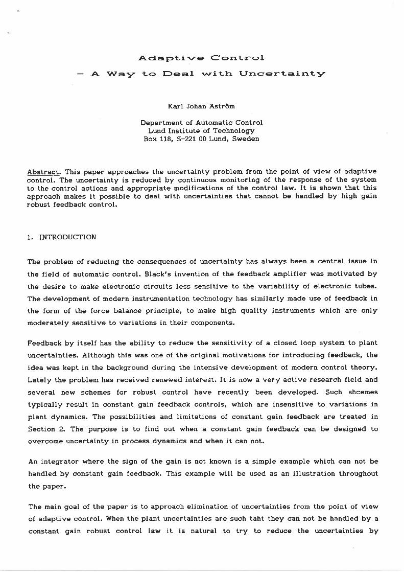
Abstract. This paper approaches the uncertainty problem from the point of view of adaptivecontrol. The uncertainty is reduced by continuous monitoring of the resPonse of the systemto the control actions and appropriate modifications of the control law. It is shown that thisapproach makes it possible to deal with uncertainties that cannot be handled by high gainrobust feedback control.

1. INTRODUCTION

The problem of reducing the consequences of uncertalnty has always been a central lssue in

the field of automatÍc sontrol. Black's invention of the feedback amplifier was motívated by

the desire to make electronic circuits less sensitive to the variabitity of elestronic tubes.

The development of modern instrumentation technology has similarly made use of feedback in

the form of the force balance principle, to make high quality instruments which are only

moderately sensitive to variations in their components.

Feedback by itself has the ability to reduce the sensitivity of a closed loop system to plant

uncertainties. Although this was one of the original motivations for introducing feedback, the

idea was kept in the background during the intensive development of modern control theory.

Lately the problem has received renewed interest. It is now a very active research field and

several new schemes for robust control have recently been developed. Such shcemes

typically result in constant gain feedback controls, whÍch are insensitÍve to variations in

plant dynamics. The possibilities and limitations of constant gain feedback are treated inSection 2. The purpose is to find out when a constant gain feedback can be designed to

overcome uncertainty in process dynamics and when it can not.

An integrator where the sign of the gain is not known is a simple example which can not be

handled by constant gain feedback. This example wÍll be used es an illustration throughout

the paper.

The main goal of the paper is to approach elimination of uncertainties from the point of view

of adaptive control. When the plant uncertainties are sucb taht they can not be handled by aconstant gain robust control law it is natural to try to reduce the uncertaintÍes by

ver

Fiqure 1. Simple feedback sYstem

experimentation and parameter estimation. Auto-tuning is a slmple technique' whfch has the

attractive feature that an appropriate input sÍgnal to the process is generated

automatically. The method has the additional benefit that parameter estimation and control

design are extremely simple to do. This is discussed in Section 3.

Auto-tuning is an intermittent procedure. The regulator has a special tuning mode, which is

invoked on the request of an operator or based on some automatíc diagnosis. Adaptive

control is a method which allows continuous reduction of the uncertalnties. An adaptive

regulator wíll continuously monitor the systems response to the control actions and modífy

the regulator appropriately. The charateristics of such control schemes are discussed in

Section 4. Two categories of adaptíve control laws, direct and indirect, are discussed in

some detail. Some theoretical results on the stabílity of adaptive control systems are

reviewed in SectÍon 5. It is found that the standard assumptions used to prove the stabilityof direct adaptive control schemes are such that robust high gaiin linear control could

equally well be apptied. Adaptive controllers are nonlinear feedback systems. There are

other types of nonlinear feedback systems, which also can deal with uncertainties. One type

is called universal stabitizer. Such a system is briefly dissussed in Section 6. Its capability

of dealing with an integrator with unknown gain is demonstrated.

Stochastic control theory is a general method of dealing with uncertainties. In Section 7 it is

shown how adaptive control laws can be derived from stochastic control theory. The example

wÍth the integrator having unknown gain is worked out in some detail.

2. LIMTTATIONS OF CONSTANT GATN FEEDBACK

Conventional feedback can deal with uncertainty in the form of disturbances and modeling

errors. Before discussing other techniques for dealing with uncertainty it is useful to

understand the possibilitíes and limitations of constant gain feedback. For thÍs purpose

consider the simple feedback system shown in Figure 1. Let GO be the nominal loop transfer

function. Assume that true loop transfer function is G = GO(l+L) due to model uncertainties.

Notice that l+L is the ratio between the true and nominal transfer functions.

Im (t.L)

Re (t*t)

Fiqure 2. The ratio between the true transfer function G(s) and the nomÍnal transferfunction GO(s) must be in the shaded region for those frequencies where GO(io) islarge.

The effect of uncertainties on the stability of the closed loop system will first be discussed.

The closed loop poles are the zeros of the equation

1+G (s) + 6 (s)L(s) - Oo o

Provided that the nominal system is stable it follows from Rouche's theorem that the

uncertainties will not cause instability provided that

lL(s) I Slr*cor"llF- (2. r,

on a contour which encloses the left half plane. The consequences of this inequality wÍIl now

be discussed. For large loop gains (2.1) reduces to

ll.(s) I 3 I

This means that the relative uncertainty l+L must be in the shaded area in Figure 2. Itfollows from Figure 2 that if the uncertainty in the phase of the open loop system is less thang in magnitude i.e.

larg(l+L) I S <9

then the closed loop system is stable provided that the magnitude of the relative uncertaintysatÍsfies

o<

For these frequencies where the loop gain is high it is thus necessary that the phase

uncertainty is less than 90o.

At the crossover frequency cr

reduces to

/2, t-coÉr .p

" where the loop gain GO(io") has unit magnitude equation (2.1)

lL ( ir¡ )ts ) (2.2)e m

where g* is the phase margin. At higher frequencies where the loop gain is less than one the

inequality (2.1) can be approximated by

lL(s) S

This means that large uncertaínties san be treated where the loop gain is significantly less

than one.

Stability is only a necessary requirement. To investigate the effect of uncertainty on the

performance of the closed loop system consider the transfer function from the command

signal to the output i.e.

lrlæt

+G Go 1+LG

o oo 1+G 1+GO+GOL o

Go1+G1 +GOL

The error in the closed loop transfer function is thus

L (2.3'c 1+GO+GOL

This error can be made small either by having a small open loop uncertaÍnty (L) or by

having a high loop gain (GO).

Equations (2.1) and (2.3) give the essence of high gain robust control. The open open loop

gain GO can be made large for those frequencies where the phase uncertainty is less than 90

degrees. At those frequencies the closed loop transfer funstion can be made arbitrarily close

to the specifications by choosing the gain sufficiently large. For those frequencies where the

uncertainty in the phase shift is larger than 90o the total loop gain must be made smaller

than one in order to maÍntain robustness. At the crossover frequency where the loop gain has

unit magnitude the allowable phase uncertainty is given by Q.21. The allowable unsertainty

depends critically on the phase margin g*. Assuming for example that it is desired to have

en error in the closed loop transfer function of at most tO% of. the crossover frequency. The

allowable phase margin is given in Table 1.

GG L

L

Table 1 - Maxfmum error in the open loop transfer function whlch glve at most 10 % error oÍthe closed loop transfer function at the crossover frequency.

9n 10 20 30 43 60

max lL I a. o77 o. o34 o. o52 o. 076 o. 100

Design techniques which can deal with uncertainty are given in Gutman

(1963), Horowitz and Sidi (1973), Leitmann (1990,1983), Kwakernaak (1985),

discussion of the multivariable case is given by Doyle and Stein (1981).

(19?9), Horowitz

çrüuet (198s). A

It is clear from the discussion above that in order to use robust high gain control it is

necessary that the transfer function of the plant has a phase uncertainty less than 90o forsome frequencies. Some examples which illustrate the limitations of high gain robust control

will now be discussed.

Example 2.1 - Time Delays

Consider a linear plant where the major uncertainty is due to variations in the time delay.

Assume that the time delay varies between Tmin "td T*"*. Furthermore assume that it is

required to keep the variations in the phase margin less than 20o. It then follows that the

cross-over frequency oc must satisfy

(,ùo.35

T Tmex mLn

The unsertainty in the time delay thus induees an upper bound to the achievable cross-over

frequency. ct

Example 2.2 - Mechanical Resonances

Mechanical resonances are associated with transfer functions of the type

2

G(s) 2È 2f,,r^lOs o

+ + (¡)

where the damping normally is very small. The phase of G changes rapidly from 0 to -1800

around oO. The gain also changes rapidly around oO. It increases from one to approximately

L/2 E and it increases ^" ,f;trz with increasing o. Variations in !, and o will thus givesubstantial phase uncertainty. To achieve robust linear control it is then necessary to make

sure that the loop gain is low around r0. This is typically achieved by a notch filter. tr

c

to2

Example 2.3 - Integrator Whose Sign is Unknown

An integrator whose sign is not known has elther a phase lag of 90o or 2?Ao. Such a system

can not be controlled using high gain robust control. c:

3. AUTO-TUNING

When the uncertafnty ls such that robust htgh gain feedback cannot be applted it ls natural totry to reduce the uncertainty by experimentation. Auto-tuning is a methodology for doing

this automatically. The principles are straightforward. A model of the process dynamics isdetermined by making an identification experiment where an input signal is generated and

applied to the process. The dynamics of the process is then determined from the results ofthe experiment. The controller parameters are then obtained from some design procedure.

Since the signal generation, the identification and the design can be made in many differentways there are many possible tuning procedures of this kind.

Auto-tuning is also useful in another context. There are ceses where is is much easier toapply an auto-tuner than to design a robust high gain controller Simple regulators with two

or three parameters can be tuned manually if there is not too much interaction between

adjustments of different parameters. Manual tuning is, however, not possible for more

complex regulators. Traditionally tuning of such regulators have followed the route of

modeling or identification and regulator design. This is often a time-consuming and costlyprocedure which can only be applied to important loops or to systems whish are made inlarge quantities.

Most adaptÍve techniques can be used to provide automatic tuning. In such applications the

adaptation Ioop is simply switched on and perturbation signals may be added. The adaptiveregulator is run untíl the performance is satisfactory. The adaptation loop is then

disconnected and the system is left running with fixed regulator parameters. Below we willdiscuss a specific auto-tuner which requires very little prior information and also has the

interesting property that it generates an appropriate test signal automatically. This isdiscussed further Ín Âstrõm and Hägglund (1984a). A nice feature of the technique dessrÍbed

below is that an input signal is generated automatically and that the parameter estimationand the control design are very simple. The input signal generated is automatically tuned tothe characteristics of the plant. It will have its energy concentrated around the frequencies

where the plant has phase lag of 1800.

The Basic Idea

A wide class of process control problems ean be described in terms of the intersection of the

Nyquist curve of the open loop system with the negative real axis, which is traditionally

T

0

-I

0 10 20 30 40Fiqure 3. Input and output signals for a linear system under relay control. The system has

the transfer function G(s) = 0.5(1-s)/s(s+1)(s+1).

described in terms of the critical gain k, and the critical period Tc. A method for

determining these parameters was described in Ziegler and Nichols (1943). It is done as

follows: A proportional regulator is connected to the system. The gain is gradually increased

until an oscillation is obtained. The gain when this occurs is the critical gain and the

frequency of the ossillation is the critical frequency. It is, however, diffÍcult to perform

this experiment in such a way that the amplitude of the oscillation is kept under control.

Relay feedback is an alternative to the manual tuning procedure. If the process Ís connected

to a feedback loop there will be an oscillation as is shown in Figure 3. The period of the

oscillation is approximately the critical period. The process gain at the corresponding

frequency is approximately given by

2nTpG t t-

etr=- 4dl (3. 1)

where d is the relay amplitude and a is the amplitude of the oscillation.

A simple relay control experiment thus gives the desired information about the process. This

method has the advantage that it is easy to sontrol the amplÍtude of the limit cycle by an

appropriate choice of the relay amplitude. A simple feedback from the output amplitude tothe relay amplitude makes it possible to keep the output amplitude fixed during the

experiment. Notice also that an input signal which is almost optimal for the estimation

problem is generated automatically. This ensures that the critical point can be determined

accurately.

When the critical point on the Nyquist curve is known, it is stralghtforward to apply the

classÍcal Ziegler-Nichols design methods. It is also possible to devise many other design

schemes that are based on the knowledge of one point on the Nyquist curve. The procedure

can be modified to determine other points on the Nyquist curve. An integrator may be

connected in the loop after the relay to obtain the point where the Nyquist curve Íntersects

Relay

PID

Process

-1

IuA

T

Fiqure 4. Block díagram of an auto-tuner. The system operates as a relay controller in thetuning mode (T) and as an ordinary PID regulator in the automatic control mode(A).

the negative imaginary axis. New design methods, which are based on such experiments, aredescribed in .4ström and Hägglund (1984b).

Methods for automatic determination of the freguency and the amplitude of the oscillationwill be given to complete the description of the estimation method. The period of an

oscillation can be determined by measuring the times between zero-crossings. The amplitudemay be determined by measuring the peak-to-peak values of the output. These estimationmethods are easy to implement because they are based on counting and comparisons only.More elaborate estimatÍon schemes like least squares estimatlon and extended Kalmanfiltering may also be used to determfne the amplitude and the freguency of the lÍmit cycleoscillation. SÍmulations and experiments on industrial processes have indicated that little isgained in practÍce by using more sophisticated methods for determining the amplitude andthe period.

A block dÍagram of a control system with auto-tuning is shown in Fígure 4. The system can

operate in two modes. In the tuning mode a relay feedback is generated as was discussedabove. When a stable limit cycle is established its amplitude and period are determined as

described above and the system is then switshed to the automatic control mode where a

conventional PID control law is used.

Practical Aspects

There are several practical problems which must be solved in order to implement an

auto-tuner. It is e.g. necessary to account for measurement noise, level adjustment,saturation of actuators and automatic adjustment of the amplitude of the oscillation. It may

be advantegeous to use other nonlinearities than the pure relay. A relay with hysteresis

gives a system which is less sensitive to measurement noise.

Measurement noise may give errors in detection of peaks and zero crossings. A hysteresls in

the relay is a simple way to reduce the influence of measurement noise. Filtering is another

possibility. The estimatÍon schemes based on least squares and extended Kalman filtering can

be made less sensitive to noíEe. Simpte detection of peaks and zero crossíngs in comblnatÍon

with an hysteresis in the relay has worked very well in practice. See e.g. Aström (1982).

The process output may be far from the desired equilibrium condition when the regulator is

switched on. In such cases it would be desirable to have the system reach its equilibrium

automatically. For a process with finite low-frequeney gain there is no guarantee that the

desired steady state will be achieved with relay control unless the relay amplitude is

sufficiently large. To guarantee that the output actualty reaches the reference value' it may

be necessary to introduce manual or automatic reset-

It is also desirable to adjust the relay amplitude automatically. A reasonable approach is to

require that the oscillation is a given percentage of the admissible swing in the output

signal.

Auto-Tuninq with Learninq

Auto-tuning is a simple way to reduce uncertainty by experimentation. In many cases the

characteristics of a process may depend on the operating conditions. If it is possible to

measure some variable whích correlates well with the changing process dynamics it is

possible to obtain a system with interesting characteristics by combining the auto-tuner

with a tabte look-up function. When the operating condition changes a new tuning is

performed on demand from the operator. The resulting perameters are stored in a table

together with the variable which characterizes the operating condition. When the process has

been operated over a renge covering the operating conditions the regulator parameters can

be obtained from the table. A new tuning is then reguired only when other conditions change.

A system of this type is semi-automatic because the decision to tune rests with the operator.

The system will, however, continue to reduce the plant uncertainty.

4. ADAPTIVE CONTROL

Adaptive control is another Ìvay to deal with uncertainties. A block-diagram of a typical

adaptive regulator is shown in Figure 5. The system can be thought of as composed of two

loops. The inner loop consists of the process and an ordinary linear feedback regulator. The

parameters of the regulator are adjusted by the outer loop, which is composed of a recursive

parameter estimator and a design calculation. To obtain good estimates it may also be

Process þarameters

Regulatorþarameters

U6

Fiqure 5. Block diagram of an adaptÍve regulator

necessary to introduce perturbation signals. This function is omitted from the fÍgure forsimplicity. Notice that the system may be reviewed as an automation of process modeling

and design where the process model and the control design is updated at each sampling

period.

The block labeled fregulator design" in Figure 5 represents an on-line solution to a design

problem for a system with known parameters. This underlying design problem can be solvedin many different ways. Design methods based on on phase- and amplÍtude margins,pole-placement, minimum variance control, linear quadratic gaussian control and otheroptÍmization methods have been considered, see Astrõm (1983). Robust design techniques can

of course also be used.

The adaptive regulator also contains a recursive parameter estimator. Many differentestimation schemes have been used, for example stochastic approxfmation, least squares,

extended and generalized least sguares, instrumental variables, extended Kalman filteringand the maximum liketihood method.

The adaptíve regulator shown in Figure 5 is called indirest or explicit because the regulatorparameters are updated indirectly via estimation of an explicit process model. It issometimes possible to reparameterize the process so that it can be expressed in terms of the

regulator parameters. This gives a significant simplification of the algorithm because thedesign calsulations ere eliminated. In terms of Figure 5 the block labelled design

calculations disappears and the regulator parameters are updated directly. The scheme isthen called a direct scheme. Direct and indirect adaptive regulators have differentproperties which is illustrated by an example.

Design

Regulator

Estimation

Processu

v

Example 3.1

Consider the dissrete time system descrlbed by

y(t+l) + ay(t) = bu(t) + e(t+l) + ce(t) l=... -1,O, 1,... (4' 1)

where te(t)l is a sequence of zero-mean uncorrelated random variables. If the parameters a,

b and c are known the proportÍonal feedback

u(t) = - Oy(t) = i: Y(t) (4.2)

minimizes the variance of the output. The output then becomes

y(t) = e(t) (4.3)

This can be concluded from the fotlowing argument. Consider the sit-uation at time t. The

variable e(t+l) is independent of y(t), u(t) and e(t). The output y(t) is known and the signal

u(t) is at our disposal. The variable e(t) can be computed from past inputs and outputs.

Choosing the variable u(t) so that the terms underlined in equation (4.1) vanishes thus makes

the variance of y(t+l) as small as possible. This gives (4.2) and (4.3). For further details' see

.{ström (1970).

Since the process (4.1) is characterized by three parameters a straightforward explicit

self-tuner would require estimation of three parameters. Estimation of the parameter c is

also a nonlinear problem. Notice, however, that the feedback law is characterized by one

parameter only. A self-tuner which estimates thÍs parameter can be obtained based on the

model

y(t+1)=Oy(t)+u(t) (4.4'

The least squares estÍmate of the parameter 6 in this model is given by

T y(k) ty(k+1) - u(k)l

e(t) k=l (4.5)

T Y (k)2

k=1

and the sontrol law is then given by

u(t) = - e(t)y(t) (4.6)

The self-tuning regulator given by (4.5) and (4.6) has some remarkable properties which can

be seen heuristically as follows. Equation (4.5) can be written as

t

t

ttty(t+1)y(t) I I t 2

t t t te(t) - 9(k) ly (k)k=1 k=1 k=1

Assuming that y is mean square bounded and that the estimate O(t) converges as t + o we get

I T (4.7't y(k+l)y(k) = Q

k=1

The adaptive algoríthm (4.5), (4.6) thus attempts to adjust the parameter ê so that the

correlation of the output at lag one is zero. If the system to be controlled is actuallygoverned by (4.1) it follows from (4.3) that the estimate will converge to the minimum

variance control law under the given assumption. This is somewhat surprising because the

structure of (4.4) which was the basis of the adaptive regulator is not compatible with the

true system (4.1). More details are given in Âström and Wittenmark (1973,1985) c¡

IndÍrect AdaptÍve Control

An advantage of indírect adaptive control is that meny dífferent desígn methods can be used.

The key issue in analysis of the indirect schemes Ís to show that the parameter estimates

converge. This will in general require that the model structure used is appropriate and thatthe input signal is persistently exciting. To ensure this it may be nesessary to introduceperturbation sígnals. Provided that proper excitation is provided there are no difficulties incontrolling an integrator whose gain may have different sign.

Direct Adaptive Control

The direct adaptive control schemes may work well even if the model structure used is not

correct as wa shown in Example 3. 1. The direct schemes will, however, require other

assumptions. Assume e.g. that the process to be controlled can be described by

A(q)y(t) = B(q)u(t) + v(t) (4.8)

where u is the input, y is the output, v is a disturbance and A9q) and B(q) are polynomials inthe forward shift operator. Stability of adaptive control of (4.8) have been given by Egardt(1979)' Fuchs (L979r, Goodwin et al. (1980), Gawthrop (1980), de Larminat (1979), Morse (1980),

and Narendra et al. (1980). So far the stability proofs are available only for some simplealgorithms. The following assumptions are crucial:

1 T

(.A1)

(A2t

I re(r tyz<*t - u(k)y(k) r

the relative degree d = deg A - deg B is known,

the sign of the leading coefficient bO of the polynomial B(q) is known,

tlin

(á,3)

(.â'4)

the estlmated model ls at least of the same order ag the processt

the polynomlal B has all zeros inslde the unlt disc.

The assumption A1 means that the time delay is known with a precision, which corresponds to

a sampling period. This is not unreasonable. For continuous time systems the assumption

means that the Together with assumption (42) it also means that the phase ís known at high

freguencies. tf this is the cese, it is possible to design a robust high gain regulator for the

problem, see Horowitz (1963), Horowitz and Sidi (1973), Leitmann (1979) and Gutman (1979).

For many systems like flexible aircraft, electromechanical servos and flexible robots, the

main difficulty in control is the uncertainty of the dynamÍcs at high frequencÍes, see Stein( 1980).

Assumption A3 is very restrÍctive, since it implies that the estimated model must be at least

as complex as the true system, whích may be nonlinear with distributed parameters. Almost

all control systems are in fact designed based on strongly simplified models. High freguency

dynamics are often neglected in the simplified models.

Assumption A4 is also crucial.. It arises from the necessity to have a model, which is linear

in the parameters in the direct schemes.

5. ROBUST ADAPTIVE CONTROL

For a long time the research on stabilÍty of adaptive control systems focussed on proofs of

global stability for all values of the adaptation gain. The results obtained under such

premises are naturally quÍte restrictlve. To get some insight into thÍs consider a continuous

time system described by

Y = G(P)u (5. 1)

where u is the input, y is the output, G Ís the transfer function of the system and p = d/dt isthe dífferential operator. Consider also the model reference adaptive control law given by

Tu=S I

(5.2)

e=v-v' 'm

where y is the desired model output, e the error and O a vector of adjustable parameters.'mThe components of the vector g are functions of the command signal. In a simple case, where

the regulator Ís a combination of a proportional feedback and a proportional feedforwardr g

becomes

deãT= - l{9e

g=[r-yl T

where r Ís the reference signal.

It follows from (5.1) and (5.2) that

$?- kerc(plsrer = ksy, (5.3)

This equation gives insÍght into the behavior of the system. Assume that the adaptation loop

is much slower than the process dynamics. The parameters then change much slower than the

regression vector g and the term OtplgTe in (3.3) can then be approximated by its averaçJe

i.e.

etplgTe ^s tG(plgTtel :e (5.4)

where rt-rt denotes time averages. Notice that the regression vector g depends on the

paremeters. The following approxÍmation to (5.3) Ís obtained

(5.5)

This is the normal situation because the adaptive algorithm is motivated by the fact the

parameters change slower than the other variables in the system under this assumption.

Notice, howerer, that it is not easy to guarantee that the parameters change slowly bychoosing k sufficiently small.

Equation (5.4) is stable if kgf CtplqTl is positive. This is true e.g. if G is strictly positivereal and if the input signal is persistently exciting. However, if the transfer function G(s) isstrictly positive real it is also possÍble to design a robust high gain feedback for the

system. We thus arrive at the paradox that the assumption required to show stability of the

adaptive system will allow the design of a robust feedbask. The assumption that G(s) isstrictly positive real is, however, not necessary as is shown by the following example.

Example 5.1

Consider a system where only a feedforward gain is adjusted and let the command signal be

a sum of sinusolds i.e.

og+ - ke(€)t'(pleTrelte o ksYm

f aosin ( oot )

n

r(t)k=1

Using the model reference algorithm given by (5.2) the parameter estimates satísfy

Assuming that the gain ls small and uslng everagês we find that the estímates are

approximately glven by

g9=krtl-el6(p)rctt

q9 = katlctt - el (5.6)

where

n(5.7 )

2k=1

The equation (5.6) is stable if a Ís posítive. Consider fírst the case of a slngle sinusoÍdal,

D = 1r the equation is then unstable if the frequency of the command signal is chosen so that

G(it¡_) has a phase-shift larger than 90o. If the input contains several frequencies it isn

necessary that the dominating contribution to (5.7) comes from frequencíes where the phase

of G(it¡) is less than 90o. ct

6. UNIVERSAL STABILIZERS

Adaptive control systems are nonlinear systems with a special structure. They are often

designed based on the idea of automating modelÍng and desÍgn. It is natural to ask if there

are other types of nonlinear sontrols whÍch also can deal with uncertainties in the process

model. A special class of systems wêre generated as attempts of solving the followingproblem which was proposed by Morse (1983). Consider the system

ü.dt =aY+bu

where a and b are unknown constants. Find a feedback law of the form

u = f (9, y)

dgm = g(0, y)

which stabilizes the system for all a and b. Morse conjectured that there are no rational fand g which stabilize the system. Morse's conjecture was proven by Nussbaum (1983) who

also showed that there exist nonrational f and g which stabilize the system, e.g. the

following functions

a 1 T eos[arg G(it^rn)I2é-l<

à

SA.èJo

è)

aL\a(J

I

0

0*¡È

c¡'ÈòS

-1

2

-4

-5

20 e-L\)\)

\3¡-s

I

00123 0r23

Fiqure 6. Simulation of an integrator with Nussbaum's control law.

f (g, y) = yêzeos I

g(o, y) 2v

This correspond to proportional feedback with the gain

k = e2sog g

Figure 6 shows a simulation of this control law applied to an integrator with unknown gain.

Notice that the regulator is initÍalized so that the gain has the wrong sign. In spíte of thisthe regulator recovers and changes the gain appropriately. Nussbaum's regulator is ofconsiderable principal interest because it shows that the assumption A2 is not necessary.

The control law is, however, not necessarily a good control law in a practical situationbecause it mãy generate quite violent control actions. The inÍtial conditions for the

simulation shown in Figure 6 were chosen quite carefully.

7. DUAL CONTROL THEORY

UncertaÍnties can also be captured using nonlinear stochastÍc control theory. The system and

its environment are then described by a stochastis model. To do so the parameters are

introduced as state variables and the parameter uncertainty is modeled by stochasticmodels. An unknown constant is thus modeled by the differential eguation

Uçu

Fiqure ?. Block diagram of an adeptive regulator obtained from stochastic control theory.

v

3?=0

with an initial distribution that reflects the parameter uncertainty. Parameter drift is

modeled by adding random variables to the right hand sides of the equations. A criterion isformulated as to minimize the expected value of a loss function, which Ís a scalar functÍon of

states and controls.

The problem of fínding a control, which minimizes the expected loss function, is diffÍcult.Under the assumption that a solution exists, a functional equation for the optimal loss

function can be derived using dynamic programming, see Bellman (1957,1961). The functional

equation, which is called the Bellman equation, is a generalÍzation of the Hamilton-Jacobi

equation in classical variational salculus. It can be solved numerically only in very simple

cases. The strusture of the optimal regulator obtained is shown in Figure 7. The controller

can be thought of as composed of two parts: a nonlinear estimator and a feedback regulator.

The estimator generates the conditíonal probability distribution of the state from the

measurements. ThÍs dístribution is called the hyperstate of the problem. The feedback

regulator is a nonlinear function, which maps the hyperstate into the spece of control

variables. This function can be computed off-line. The hyperstate must, however, be updated

on-line. The structural simplicity of the solution is obtained at the price of introducing the

hyperstate, which is a quantity of very high dimension. Updating of the hyperstate requires

in general solution of a complicated nonlinear filtering problem. Notice that there is no

distinction between the parameters and the other state variables in Figure 7. This means that

the regulator can handle very rapid parameter variations.

The optimal control law has interesting properties whieh have been found by solving a

number of specific problems. The control attempts to drive the output to its desired value,

but it will also introduce perturbations (probing) when the parameters are uncertain. This

improves the quality of the estimates and the future controls. The optimal control gives the

correct balanse between maintaining good control and small estimation errors. The name dual

Nonlinearfunction

Hyþerstate

Process

Calculationof

hyþerstate

control was coined by Feldbaum (1965) to express this property. Optimal stochastíc controltheory also offers other possibilities to obtain sophlsticated adaptive algorithms, see

Saridis (L977r.

It is interesting to compare the regulator in Figure 7 with the self-tuning regulator inFigure 5. In the adaptive regulator the states are separated into two groups, the ordinarystate variables of the underlying constant parameter model and the parameters which areassumed to vary slowly. In the optimal stochastic regulator there is no such distinction.There is no feedback from the variance of the estimate in the adaptive regulator although

this information is avaílable in the estimator. In the optimal stochastic regulator there isfeedback from the condÍtional distribution of parameters and states. The design calculations

in the adaptive regulator is made in the same way as if the parameters were known exactly.Finalty there are no attempts in the adaptive regulator to introduce the estimates when theyare uncertain. In the optimal stochastic regulator the control law is calculated based on thehyperstate which takes full account of uncertainties. This also introduces perturbatÍons when

estimates are poor. The comparison indicates that it may be useful to add parameter

uncertainties and probing to the adaptive regulator. A simple example íllustrates the dual

control law and some approximations.

Example 7.1

Consider a discrete time version of the integrator with unknown gain

y(t+1) =y(t) +bu(t) +e(t),

where u is the control, y the output and e normal (0ro") white noise. Let the crÍterion be tominimize the mean square deviation of the output y. This Ís a special case of the system inExample 3.1 with a = 1 and c = 0. When the parameters are known the optimal control law isgiven by (3.2) i.e.

(7. L'

(7.2'u(t) y(t)b

If the parameter b is assumed to be a random variable with a Gaussian prior distribution, the

conditional distribution of b, given inputs and outputs up to time t, is Gaussian with mean

b(t) and standard deviation d(t). The hyperstate is then charaeterized by the triple(y(t)rb(t),o(t)). The equations for updating the hyperstate are the same as the ordÍnaryKalman filtering equations, see Âström (19?0) and (1978).

Introduce the loss function

t+NVN -2 min E

\-2Lv Yt=ct euk=t+ I

(k) (7.3'

$rhere Y, denotes the data avaltabte at tlme t l.e. (y(t), y(t-l)r...). By lntroducing the

normallzed varlables

n - y/6., I = b/cÍ, tr -ur./y (7. 4'

it can be shown that V* depends on q and p only. The Bellman equation for the problem can

be wrÍtten as

Vr(q, p) = min UT(n, Ê, p) (7.3'

where

v (q,Ê) = oo

and

2U (n, Ê, p) ( n-pn ) +1+

T

where g is the normal probability density and

y=rì-pn+e / 1+ tË"1

2b= une

p +Ft 1+ tË"1

tË"1' * f vr-r(v, b)e(e)de 0'6'qt

- att

2

e

2pl(n,P) = arg min ( n-pn) +1+

sÉ.n

see .{strðm (1978}. When the minÍmization is performed the control law is obtained as

pT(n,P) = âFg min U, (n,Ê,t¡)

The minimization can be done analytically for T = 1. We get

(7.7 '

tË"]'] _LL*þ2

Transforning back to the original variables we get

u(t) (7.8)

This control law is called one-step control or myopic control because the loss function V,

only looks one step ahead.

I=-b(t)

û2ttrôât

bt(t)+6'<t)

For T > 1 the optimization can no longer be made analytically. lnstead we have to resort tonumerical calculations. For large values of T the solutlon can be approxfmated by

o. s6Ê +9,2 1.99p(n, þ) 2 +4 n>

2.2+0.089+p q(1.7 + P

The control law is an odd function in r¡ and p, see Âström and Helmersson (1983).

Some approximations to the optimal control law will also be dÍscussed. The certainty

equivalence control

u(t) - y(l)/b (7-9)

is obtained simply by takÍng the control law Q.24) for known parameters and substitutÍng the

parameters by their estimates. The self-tuning regulator can be interpreted as a certainty

equivalence sontrol. Using normalized variables the control law becomes

t¡ I (7.9',)

The myoplc control law (7.8) Is another approximation. This is also called cautlous control,

because in comparison with the certainty equivalence control Ít hedges and uses lower gain

when the estimates are uncertaln. Notice that all control laws are the same for large p i.e ifthe estimate is accurate. The optimal control law is close to the cautious control for large

control errors. For estimates with poor precision and moderate control errors the dual

control gives larger control ections than the other control laws.

A simulation of the dual control law for an integrator with variable gain is shown in Figureg. Notice that the gain varies by an order of magnitude Ín size and that it changes sign at

T = 2000. In spite of this the regulator have littte difficulty in controllíng the process. Also

notice that the regulator does probing well before the gain changes tÍme and that it jumps

between cautÍon and probing when the gain pesses through zero.

0

5

0

à

a.

o

è)

oL

s()

<-s-si

s

I

0

0 1000 2000 4000

Fiqure 8. Simulation of dual control law applled to integrätor wlth variable gain.

REFERENCES

Âström, K.J. (1970). Introduction to Stochastic Control Theory. Academic Press, New York.Âström, K.J. (1978). Stochastic Control Problems. In Coppel, W.A. (Ed.). Mathematical Control

Theory. Lecture Notes in Mathematics' Springer-Verlag' Berlin.Âström, K.J. (1982). Ziegler-Nichols auto-tuners. Report CODEN: LUTFD2/TFRT-3167, Dept. of

AutomatÍc Control, Lund Institute of Technology, Lund' Sweden.Âström, K.J. (1983). Theory and applícations of adaptive control - A survey. Automatica, vol.

19, pp. 4lt-487, t993.Âström, K.J., and T. Hägglund (1984a). Automatic tuning of simple regulators. Proceedings

IFAC 9th World Congress, Budapest, Hungary.Âstrõm, K.J., and T. Hägglund (1984b). Automatic tuning of simple regulators with

specifications on phase and amplitude marglns. Automatica, vol. 20, No. 5, Special Issueon Adaptive Control, pp. 645-651.

Âström, K.J., and B. Wittenmark (1973). On self-tuning regulators. Automatica, vol. 9, pp.185-199.

Aström, K.J., and B. Wittenmark (1985). The self-tuning regulators revisited. Proc. ?th IFACSymp. IdentifÍcation and System Parameter Estimation, York, UK.

BeIIman, R. (195?). Dynamic Programming. Princeton University Press.Bellman, R. (1961). Adaptive Processes - A Guided Tour. Princeton University Press.Doyle, J.C and G. Stein (1981). Multivariable feedback design: Concepts for a

Classical/Modern Synthesis. IEEE Trans. Aut. Control, vol. AC-ãO, pp. 4-16.

2

T

0

-1

10

3000

Egardt, B. (19?9). Stability of Adaptive Controllers. Lecture notes in Control and InformationSciences, Vol. 20' Springer-Verlag, Berlin.

Feldbaum, A.A. (1965). Optimat Control System. Academic Press, New York.Fuchs, J.J. (19?9). Commande adaptative directe des systemes linéaires discrets. These D-E-'

Univ. de Rennes, France.Gawthrop, P.J. (1980). On the stability and convergence of a self-tuning controller. Int. J.

Control, vol. 31, pp. 973-998.Goodwin, G.C., P.J. Ramadge, and P.E. Caines (1980). Discrete-time multivariable adaptive

control. IEEE Trans. Aut. Control, vol. AC-25, PP. 449-436-Grübet, G. (1985). Research on uncertainty and control at DFVLR. This symposium.Gutman, S. (19?9). Uncertain dynamical systems - Lyapunov min-max approach. IEEE Trans-

Aut. Control, vol. 24, pP. 437'443.Horowitz, I.M. (1963). Synthesis of Feedback Systems. Academic Press, New York.Horowltz, I.M., and M. Sidi (19?3). Synthesis of cascaded multipleloop feedback systems with

Iarge plant parameter ignorance. Automatica, vol. 9, PP. 599-600-Kwakernaak, H. (1985). Uncertain models and the design of robust control systems- This

symposium.Larminat, Ph. de (19?9). On overall stability of sertaín adaptive control systems. sth IFAC

Symp. on ldentification and System Parameter Estimation, Darmstadt' FRG.Leitmann, G. (19?9). Guaranteed asymptotic stabilíty for some linear systems with bounded

uncertainties. J. Dyn. Syst. Meas. Control, vol. 101, pp- 212-2t6.Leitmann, G. (1980). Þeterministic control of uncertain systems. Astronautica Acta, vol. 7'

pp. 1457-1461.LeÍtmann, G. (1983), Deterministic control of uncertaín systems. Proc. 4th Int. Conf.

Mathematical Modelling, Zurich. Pergamon Press' Ltd-Morse, A.S. (1980). Global stabilÍty of parameter-adaptive control systems. IEEE Trans- Aut.

Control, vol. AC-25' pp.433-439.Morse, A.S. (1983). Recent problems in parameter adaptive control. tn I.D. Landau, Ed-'

Outils et Modeles Mathematiques pour l'Automatique, l'Analyse de Systemes et leTraitement du SÍgnal. Editions NRS, vol. 3, pp. 733-?40.

Narendra, K.S., Y.-H. Lln, and L.S. Valavani (1980). Stabte adaptive controller design - PartII: Proof of Stability. IEEE Trans. Aut. Control, vol. AC-25, pp. 440-448.

Nussbaum, R.D. (1983). Some remarks on a conJecture in parameter adaptlve control. Systemsand Control Letters, vol. 3, PP. 243-246, t983.

Saridis, G.N. $977r. SeLf-Organizing Control of Stochastic Systems. Marcel Dekker, NewYork.

Stein, G. (1990). Adaptive flight control: A pragmatic víew. In K.S. Narendra and R.V.Monopoll, Eds., Applications of Adaptive Control. Academic Press, New York' pp.29t-3t2.

ZIegLer, J.G., and N.B. Nichols (1943). Optimum settings for automatic controllers. Trans.ASME, vol. 65, pp. 433-444.