Adaptive bandwidth provisioning with explicit respect to QoS requirements

Adaptive bandwidth provisioning with explicit

respect to QoS requirements*

Hung Tuan Tran*, Thomas Ziegler

Telecommunications Research Center Vienna (ftw.), Donaucity Strasse 1, 1220 Vienna, Austria

Received 28 October 2003; revised 17 December 2004; accepted 20 December 2004

Available online 7 January 2005

Abstract

We propose adaptive bandwidth provisioning schemes enabling quality of service (QoS) guarantees. To this end, we exploit periodic

measurements and traffic predictions to capture closely traffic dynamics. We make use of the Gaussian traffic model providing bounds for

QoS to derive the associated bandwidth demands. Moreover, special attention is paid to alleviating some typical problems with adaptive

provisioning like QoS degradations and signaling overhead. Analytical and simulative investigations using real traffic traces show that the

proposed schemes outperform previous ones.

q 2005 Elsevier B.V. All rights reserved.

Keywords: Bandwidth provisioning; Statistical QoS; Gaussian process

1. Introduction

QoS-aware bandwidth provisioning is certainly an

important issue regarding the profitable operation of service

providers. Network operators would like to attract custo-

mers by committing to QoS delivery, but at the same time

they prefer reasonable bandwidth provisioning, rather than a

too plentiful over-provisioning. Toward this two-fold aim,

QoS-aware adaptive bandwidth provisioning schemes

emerge as a promising solution having a wide range of

applicability. Plausible examples are QoS-aware bandwidth

allocation for traffic classes in the DiffServ architecture,

QoS-aware resizing of tunnels (e.g. MPLS tunnels, tunnels

in Virtual Private Networks, logical links in the Service

Overlay Networks [1] for providing end-to-end QoS over

inter domains), and QoS-aware capacity design for IP links.

Most of the work on bandwidth provisioning so far

simply use the link utilization as a basic factor for

0140-3664/$ - see front matter q 2005 Elsevier B.V. All rights reserved.

doi:10.1016/j.comcom.2004.12.020

* An earlier, abridged version of this paper appeared in the proceedings of

the 4th COST 263 International Workshop on Quality of Future Internet

Services, QoFIS’03.

* Corresponding author. Tel.: C43 1 505 28 30/50; fax: C43 1 505 28

30/99.

E-mail addresses: [email protected] (H.T. Tran), [email protected] (T. Ziegler).

provisioning. It means that a certain target link utilization

threshold (e.g. 50 or 70%, solely based on practical

experiments) is adopted, and bandwidth is added to or

released from the link based on the relation between the

current link utilization and the target threshold. In fact, this

kind of provisioning solution is widely used in practice by

backbone service providers [2], by VPN operators [3], and

by overlay network providers [1].

The drawback of the link utilization based provisioning

solution above is that the role of the adopted utilization level

on QoS achievements is not explicitly specified. In other

words, if we are given a QoS requirement, saying, e.g. that

only 1% of packets is allowed to encounter a delay

exceeding 10 ms, we do not know how to choose the right

value of the corresponding link utilization for provisioning

purpose.

The above observation gives us a motivation to elaborate

novel provisioning schemes with explicit respect to

statistical QoS requirements. Our main contribution in this

paper is the specification of how to adjust adaptively the

bandwidth of a given link to meet the given requirements on

objective QoS parameters, like packet loss and packet delay

probabilities. We develop novel adaptive provisioning

schemes whose features are based on traffic measurements,

the Gaussian traffic model, and appropriate traffic

Computer Communications 28 (2005) 1862–1876

www.elsevier.com/locate/comcom

http://www.elsevier.com/locate/comcom

H.T. Tran, T. Ziegler / Computer Communications 28 (2005) 1862–1876 1863

predictors. By testing the proposed schemes with real traffic

traces, and applying a well-defined analytical assessment

methodology, we show that they exhibit superiority over

some existing schemes, and indeed serve as promising

candidates for resource management tasks.

The paper is organised as follows. In Section 2, we

explain the specific details of our provisioning task and

propose two new provisioning schemes referred to as PS1

and PS2. Afterwards, in Section 3 we assess the perform-

ance of these two schemes. We work out the methodology

for the quantitative assessment and based on that, achieve

the performance evaluation in comparison with existing

provisioning alternatives using real traffic traces. The

detailed analysis of the obtained results in this section

triggers further enhancements of the proposed schemes.

Thus, in Section 4 we develop additional rules supporting

signalling overhead reduction. Also, we develop new traffic

prediction rules to avoid under-estimation of traffic, leading

to two new provisioning schemes referred to as PS1* and

PS1**. We demonstrate by trace driven simulation and by

theoretical arguments (the strict proof is found in Appendix

A) that these enhanced schemes indeed achieve much better

results than the existing schemes. In Section 5, we envision

some typical application areas of the proposed provisioning

schemes. In Section 6, we provide a brief overview on

related work, pointing out the added value of our schemes.

Finally, Section 7 concludes the paper.

2. Development of QoS-aware, adaptive provisioning

schemes

Our main provisioning task is to determine the

bandwidth allocated to the link satisfying the target QoS,

which is the packet level constraint

PrðdelayODÞ!e: (1)

Here, D and e are the given delay bound (excluding the

propagation delay) and the upper-bound for the violation

probability, respectively. Moreover, for economical band-

width usage, the bandwidth allocation should be done with

respect to the dynamics of the traffic the link accommo-

dates. In other words, we aim to achieve dynamic

provisioning, where the needed bandwidth amount is

adaptively adjusted from time to time, taking into account

the dynamics of the accommodated traffic. The total delay

is composed of queueing delay and transmission delay.

However, when the packet size is considerably small

compared to the link capacity c (which is particularly true

for high speed links), the transmission delay negligibly

contributes to the total delay. Thus, we can consider the

delay constraint (1) equivalent with the constraint on the

queue tail probability

PrðQODcÞ!e; (2)

where Q stands for the queue length, and c is the

bandwidth to be allocated.

In Section 2.1, we first briefly describe an estimation of

the queue tail probability (2), and then we present our two

preliminary provisioning schemes based on this estimation.

2.1. Estimation of the queue tail probability

using the Gaussian traffic model

For high speed links accommodating a huge number of

traffic flows, QoS-aware provisioning rules based on the

exact traffic description derived from exact characteristics

of individual flows collapse in a sense of practical

applicability. It is due to the exploration of state space

one could face. Therefore, an assimilated and tractable

model for the aggregate traffic should be preferred. From

this point of view, the Gaussian process has recently been

considered as a good candidate because it captures well

characteristics (multiplexing effects, correlation structure)

of the aggregate traffic while still being easily controllable

[4–6].

Specifically, [5] proposes the so called MVA (Maximum

Variance Asymptotic) bound for the tail probability of the

buffer fed by an input Gaussian process. Moreover, it is

shown therein that this asymptotic bound practically

behaves like a tight global upperbound for the queue tail

probability. Ref. [6] utilizes the MVA bound along with the

exact loss probability of a bufferless system to give an

estimation on the loss probability of a given system with a

finite buffer. Both papers present an analysis based on a

discrete time, fluid-flow queue which we briefly summarize

below.

Given a queue with the aggregate input rate ln and

service rate c at time n, define a stochastic process Xn as

Xn ZXn

kZ1

lk Kcn: (3)

For a buffer size x, define the normalized variance s2x;n of

Xn as

s2x;n :Z

VarfXng

ðx KEfXngÞ2; (4)

and let sx be the reciprocal of the maximum of s2x;n, i.e.

sx :Z1

maxnR1s2x;n

: (5)

We note that if the aggregate input rate ln is a Gaussian

process, so is Xn. Using the Gaussian property of Xn and the

so called dominant time scale approach [5], the MVA

bound, i.e. the bound on the queue tail probability P(QOx),

is given as eKsx=2. We will formally write

MVA_boundðEfXng;VarfXng; xÞ Z eKsx=2: (6)

The loss estimation (i.e. the loss probability PL(x) for

buffer size x) is given as g eKsx=2 [6]. Here, the term g is

Fig. 1. A binary search to compute the needed bandwidth amount.

H.T. Tran, T. Ziegler / Computer Communications 28 (2005) 1862–18761864

calculated as

g Z1ffiffiffiffiffiffiffiffiffi

2psp eðcK�lÞ2=2s2

ðN

cðr KcÞeðrK

�lÞ2=2s2

dr;

where �lZEflng, s2ZVarflngZClð0Þ and Cl(l) is the

autocovariance function of ln.

For the given value of n, nR1, the mean and variance of

Xn can be computed from the mean and the autocovariance

functions of the input rate as

EfXng Z nð �l KcÞ (7)

VarfXng Z nClð0ÞC2XnK1

lZ1

ðn K lÞClðlÞ: (8)

The presented MVA and loss bounds can be used to make

the mapping between the bandwidth to provision and QoS

requirements explicit. In the remainder of this paper we will

present MVA bound based (or equivalently, delay-based)

provisioning schemes. However, the same concept is

straightforwardly applicable to the loss or loss-delay

combination based provisioning as well.

2.2. Provisioning schemes combining use of the Gaussian

model, periodical measurements, and traffic predictions

The incipient point of our provisioning schemes is to

collect periodically the aggregate rate of the incoming traffic

in consecutive time slots with length t. Denote the traffic

rate measured in slot i by yi. Bandwidth provisioning is

performed at a larger time scale expressed in resizing

windows (or shortly, windows). One resizing window

consists of N measurement time slots. We compute the

mean and autocovariance functions of traffic over a given

window j as mjZPN

iZ1yðjÞi

N, and

CjðkÞ Z1

N Kk

XNKk

iZ1

ðyðjÞi KmjÞðy

ðjÞiCk KmjÞ

for k Z 0; 1;.;N K1:

The computed quantities enable us to capture the mean

and variance of the accumulated traffic process Xn by using

Eqs. (7) and (8) and in turn the MVA and loss bounds. At the

end of each resizing window we make a decision about the

bandwidth amount needed for the next resizing window. We

specify two schemes for this task.

PS1 scheme, delay-based, with prediction. In this

scheme, we propose to perform traffic prediction at the

end of each resizing window for the next one. We predict

both the mean rate of the aggregate traffic and the variance

of the cumulative process Xn. We opt for the exponential

smoothing (ES) technique for the prediction due to its

proven stability and suitability on trend prediction [7].

Formally, for the resizing window jC1 we predict

m�jC1 Z wmj C ð1 KwÞm�

j ; (9)

where w is the weighting parameter (0%w%1), m�j and mj

are the predicted and measured values of the mean rate for

the resizing window j, respectively. Similarly, for the

variance of the accumulated traffic, we predict

Var�fXn;jC1g Z w VarfXn;jgC ð1 KwÞVar�fXn;jg (10)

where Var*{Xn,j} and Var{Xn,j} (nZ0,1,.,NK1) are the

predicted and measured values of the corresponding

accumulated variance for the resizing window j, respect-

ively. We then use the predicted m�jC1 and Var*{Xn,jC1}

values as the inputs for the binary search presented in Fig. 1 to

define the needed bandwidth for the window jC1. In Fig. 1,

the MVA bound computation is symbolically denoted by the

function MVA_bound( ), as introduced earlier in (6). The

output of the binary search is the bandwidth amount assuring

that the achievable QoS is sufficiently close (expressed via

the parameter e*) to the target QoS requirements.

PS2 scheme: delay-based, without prediction. In this

scheme, we simply use the computed mj and Var{Xn,j} (nZ0,1.,NK1) as the input parameters of the binary search for

the needed bandwidth of the window jC1.

3. Performance evaluation of the new provisioning

schemes

In this section, we evaluate the operation of the proposed

provisioning schemes PS1 and PS2. Before going into the

detailed investigations, we delineate the testing scenarios in

use and our assessment methodology in Section 3.1.

3.1. Scenario settings and methodology for evaluations

In order to have a comparative baseline, we involve two

other existing provisioning schemes available from previous

work. We referred to them as PS3 and PS4 schemes.


PS3 scheme: utilization-based, without prediction. In this

scheme, link bandwidth regulation is based on the relation

between the link utilization threshold and the measured link

utilization in the last resizing window. According to the

proposal of Duan et al. [1], the bandwidth amount to be added

or released is measured in quota. One quota can be set to e.g.

bffiffiffiv

p, where v is the variance of the measured traffic rate. In

accordance with [1], we set the target link utilization to 0.8

and bZ0.6.

PS4 scheme: variance-based, without prediction. In this

scheme, the provisioned bandwidth for the next resizing

window is chosen to be mjCaffiffiffiffivj

p, where mj and vj are the

mean and variance in the current window j. The reason

behind this bandwidth setting and the concrete value of a is

that the scheme ensures that the aggregate traffic rate will

only exceed the chosen bandwidth with a probability

QðaÞZ ð1=2Þerfcða=ffiffiffi2

pÞ, where erfcðxÞZ ð2=

ffiffiffiffip

pÞÐN

x eKz2

dz.

This is the scheme by Duffield et al. [3]. In accordance with

[3], we set aZ3 (corresponding to the exceeding probability

Q(a)Z1.349!10K3).

We use three real traffic traces1 to produce the aggregate

load offered to the link. The MPEG trace is the trace of a

James Bond movie available from [8]. The BC-pAug89 trace

of Ethernet traffic is available from [9]. The WAN trace is a

wide-area TCP traffic trace dec-pkt-1 available also from

[9]. To generate the aggregate traffic with high multiplexing

degree, we merge 100 individual sources having the above

recorded traffic pattern. The starting time of each individual

source is randomly chosen to assure independency between

the sources.

We examine two scenarios of provisioning as regards the

scale of basic measurement time slots and resizing windows.

Namely, we consider resizing at small time scale, when each

resizing window contains 100 measurement time slots of

length 40 ms, i.e. resizing is done after each 4 s interval. In

this case, the provisioning is tested along 100 resizing

windows, meaning that the whole period of provisioning is

400 s. With resizing at large time scale, each time slot is

1200 ms, and resizing is done after each 100 slots, i.e. after

each 2 min. In this case, we test the provisioning schemes

along 13 resizing windows, meaning that the whole period of

provisioning is approximately half an hour.

We evaluate the performance of the schemes along two

parallel analysis aspects. In the simulative analysis, we

resort to trace-driven simulation to verify and evaluate the

performability of the provisioning schemes. The basic

scenario is that traffic according to the generated aggregate

trace is accommodated via a single link. The link capacity is

adjusted after each resizing window time and a value

computed off-line with the specific provisioning scheme

is assigned. We trace both the instantaneous queue length

at the queue (placed at the near-end of the link)

1 We process the original data traces so that the load over consecutive

time intervals with fixed length, i.e. the measurement slots, can be obtained.

and the queueing delay of individual packets. This data

collection enables us to compute the delay violation

probability for any given delay bound. Simulation results

will be reported later in Section 4.3.

For the analytical analysis, in order to evaluate

quantitatively the applied provisioning schemes, we intro-

duce the notion of Average Goodness Factor (AGF). This is

a measure of how fast and closely the provisioned

bandwidth follows the real traffic dynamics, while assuring

the target QoS. The basic idea is that in an ideal

provisioning case, the link utilization should be kept

constant at a fixed optimal level uopt. The concrete value

of uopt is chosen from the experiments gained by using the

Gaussian traffic model to deduce the relation between the

objective QoS parameters and the link utilization. For a

given resizing window j, let us denote the provisioned link

capacity by lj, the real aggregate traffic rate by rj. We then

define the Goodness Factor (GF) as follows:

GFj :Z

ðlj KrjÞ=rj

uopt

if lj%rj

rj=lj

uopt

if ljOrj and rj=lj%uopt

uopt

rj=ljif ljOrj and rj=ljOuopt

8>>>>>><>>>>>>:

(11)

This definition of the GF is motivated by the following

interpretations. Consider the severe under-provisioning

case when the provisioned link bandwidth is smaller than

the real traffic rate. The provision is then considered

‘wrong’, or equivalently it has a negative GF. The closer to

the real traffic rate the link capacity is, the ‘less wrong’ the

provision (i.e. its GF still remains negative but has a smaller

absolute value). On the other hand, for a given lj and rj

(lj%rj) the larger the optimal link utilization uopt, the larger

the GF value should be (because the under-provisioning has

less detrimental effect). These arguments are reflected on

the formulae ððlj KrjÞ=rjÞ=uopt. One can check that for two

different bandwidth values lð1Þj and lð2Þj , if lð1Þj O lð2Þj , then

ððlð1Þj KrjÞ=rjÞ=uopt O ððlð2Þj KrjÞ=rjÞ=uopt. Similarly, for two

different utilizations uopt1and uopt2

, if uopt1Ouopt2

, then

ððljKrjÞ=rjÞ=uopt1O ððljKrjÞ=rjÞ=uopt2

.

Now, consider the over-provisioning case when the

provisioned link capacity is larger than the real traffic rate,

and the utilization is below the optimal one, i.e. ljOrj and

rj/lj%uopt. This means that the link is somewhat over-

provisioned and decreasing the link capacity should result in

a better provisioning scheme. In other words, in this case the

GF should increase with the decrease of the provisioned link

capacity, which is reflected in the expression ðrj=ljÞ=uopt.

Similar arguments lead to the expression GFZuopt=ðrj=ljÞ

when the provisioned link capacity is larger than the real

traffic rate, but the actual link utilization is above the

optimal one, i.e. ljOrj and rj/ljOuopt.

Note that the GF value is either negative (the first case) or

positive but smaller than 1 (the latter two cases). The AGF is

Table 1

AGF values obtained with different prediction weights w

Small time scale Large time scale

w/Traffic MPEG WAN Ethernet MPEG WAN Ethernet

0.1 0.779 0.642 0.784 0.510 0.036 0.776

0.5 0.848 0.805 0.890 0.743 0.496 0.704

0.8 0.880 0.898 0.913 0.704 0.721 0.840

0.9 0.901 0.920 0.916 0.717 0.794 0.852

0.95 0.911 0.922 0.915 0.728 0.797 0.844

1 0.915 0.913 0.914 0.648 0.790 0.836


then obtained by averaging all individual GF values over the

resizing windows, AGFZPM

1 GFj=M, where M is the

number of resizing windows. The higher the degree of over-

provisioning or under-provisioning, the smaller the AGF

value. The minimum AGF value is K1/uopt, the maximum

AGF value is 1. Moreover, the closer the AGF to 1, the

better the provisioning scheme.

Regarding the choice of the weighting parameter w used

in Eqs. (9) and (10), we have calculated the AGF values we

can obtain with the PS1 scheme for a set of w values. The

results are reported in Table 1. As the numerical values in

Table 1 indicate, for the three specific traffic aggregates,

there is a value of w between 0.8 and 1 (note that setting

wZ1 is nothing but to switch from PS1 to PS2 scheme)

yielding the maximum AGF. Nevertheless, the table also

shows that this maximum AGF value is not significantly

bigger than other AGF values obtained with other choices of

w. We have also tried with adaptive setting of w, e.g. to

adjust it accordingly to the dynamics of the relative or

absolute bias between the current traffic load value and the

predicted load value. However, our several adaptive setting

attempts do not yield noticeable improvements of PS1, at

least for the traffic patterns WAN, MPEG and Ethernet we

use. For this reason, in the rest of the paper, if not stated

otherwise, we set wZ0.8, keeping in mind that there might

be a smart adaptive setting of w further improving the

goodness of our provisioning schemes.

In addition, if not stated otherwise, we set the initial

value of the link bandwidth to 150 Mbps. The input

parameters for the binary search in Fig. 1 are:

†
the delay bound DZ10 ms,
†
the desired delay violation probability eZ10K4,
†

2 We skip the figures about Ethernet and WAN traffic traces, because they

allow the same conclusions.

e*Z0.1, allowing a range of (10K0.1, 100.1) for the QoS

bias, i.e. the QoS is considered acceptable when the

actual delay violation probability is in the range of

(0.79e, 1.25e).

3.2. Investigations on the performance

of PS1 and PS2 scheme

Figs. 2 and 3 present the small time scale provisioning

for MPEG traffic. Fig. 2 depicts the measured aggregate

rate (mj), the predicted aggregate rate (m�j ), the

bandwidth provisioned by the PS1 and PS2 schemes

vs. the resizing windows. Fig. 3 depicts the measured

aggregate rate (mj), the predicted aggregate rate (m�j ),

and the bandwidth provisioned by the PS3 and PS4

schemes. Figs. 4 and 5 are the counterpart of Figs. 2 and

3, which present the large time scale provisioning for

MPEG traffic.2

Considering the figures, we see that the PS1, PS2, and

PS4 schemes capture very well the shape of the aggregate

traffic. The three schemes react fast and closely to

variations of the aggregate rate. PS1 and PS2 schemes

exhibit nearly the same behaviour, and in fact their curves

are hardly distinguishable (see Figs. 2 and 4). The PS3

scheme does not follow well all the traffic fluctuations, but

rather has a smooth shape with linear increase or decrease.

This is in accordance with the original intention of this

approach, i.e. adjusting bandwidth insensitively to small

short-time traffic fluctuation [1]. Since PS3 reacts slowly to

the changes of the traffic, one of the consequences from

this property is that it is very sensitive to the initial

provisioned bandwidth value. Thus, it needs a long time to

reach an acceptable state where over-provisioning or

under-provisioning becomes less aggravating (see, e.g.

Fig. 3, windows 1–35).

At a larger time scale when provisioning actions are

taken at every 2 min, we see that the PS3 scheme works

unacceptably (Fig. 5). It is due to the inadequate setting of

the quota volume through the parameter b. In fact, the AGF

assessment in Table 2 confirms that with bZ0.6, the PS3

scheme exhibits the poorest performance in comparison to

PS1, PS2 and PS4 schemes. The table also shows that the

PS4 scheme, though it still captures well the tendency of

the traffic rate, is outperformed by the PS1 and PS2

schemes. The cause of such poor performance of PS3 and

PS4 relies behind the concrete choice of their parameter a

(which is currently set to 3) and b. Intuitively, appro-

priately tuning parameters a and b probably leads to better

performance of PS4 and PS3, respectively. However, if we

do not have a reasonable mapping between the QoS

requirements and the needed link utilization then there is

no way to choose the right values of a and b. Thus, PS1

and PS2 schemes with their model-based mapping features

are definitely more suitable in case explicit QoS is

required.

In Table 2, we report the AGF values of the provisioning

schemes for different traffic scenarios. The value of uopt is

set to be the average value of the utilizations achievable

over all the resizing windows with the Gaussian traffic

model to meet the target QoS requirement. To make the

comparative evaluation more complete, we also include the

AGF of the static provisioning schemes, where bandwidth is

kept constant over the whole time. In the ‘bad’ scheme

Static-1, the bandwidth is fixed at 150 Mbps. In scheme

Fig. 2. Small time scale bandwidth provision for MPEG traffic, PS1 and PS2 schemes.

Fig. 3. Small time scale bandwidth provision for MPEG traffic, PS3 and PS4 schemes.


Static-2, with the rough knowledge on the aggregate rate of

traces, the bandwidth is fixed at 70, 250 and 200 Mbps for

MPEG, WAN and Ethernet traffic, respectively. Table 2

shows that the static schemes are in general outperformed

by the rest of the schemes. Moreover, the qualitative relation

between the AGF values of the schemes confirms all our

previous arguments. The PS3 scheme works unacceptably at

large time scale provisioning. PS1 and PS2 schemes have

nearly the same goodness and they are the best among the

tested schemes.

Beside the conclusion that the QoS-aware PS1 and PS2

schemes are better than the existing ones (including PS3,

PS4, and the static ones), it is to mention that there are still

questionable issues with PS1 and PS2. These issues are

concerned with signaling overhead and under-provisioning,

which are dealt in Section 4.

4. Further enhancing our provisioning schemes

4.1. Signalling reduction

From a practical point of view, the merit of any dynamic

provisioning scheme is judged by the tradeoff between

adjustment frequency and signalling overhead. On the one

hand, the higher the provisioning frequency, the better and

more accurate the resource allocation reflects the real traffic

dynamics. On the other hand, however, more adjustments

may require more signalling overheads (negotiations on

bandwidth amount, allocation and/or release of bandwidth),

which can have detrimental impacts on network

performance.

From the macroscopic point of view, the simplest way

to reduce signalling overhead is to skip non-critical

Fig. 5. Large time scale bandwidth provision for MPEG traffic, PS3 and PS4 schemes.

Fig. 4. Large time scale bandwidth provision for MPEG traffic, PS1 and PS2 schemes.


bandwidth adjustments. Therefore, we propose the follow-

ing potential solutions for scalability improvements. For

skipping downward adjustments, we consider that over-

provisioning is always less detrimental than under

provisioning. Thus, if the relative bandwidth bias remains

below a certain value (e.g. 5% of the current bandwidth

value), we could keep the current bandwidth amount and

do not perform deallocation. By doing this, a certain range

of over-provisioning is implicitly involved at the gain of

signalling effort.

For skipping upward adjustments, we introduce a certain

number of bandwidth levels. We refer to the difference

between two consecutive bandwidth levels as a bandwidth

interval. If both the current and the new bandwidth values

stay within the same bandwidth interval, we do not initiate

the upgrade process. This is based on the compromise that

within one bandwidth interval, we can tolerate a certain

degree of QoS degradation. The procedure checking the

impact of bandwidth interval’s size on QoS degradations is

done as follows. We compute first the needed bandwidth for

the next resizing window taking the required delay violation

probability into account. Afterward, we reduce the com-

puted bandwidth by the amount identical to one bandwidth

interval size and then recompute the delay violation

probability we should get. We use the ratio between the

recomputed violation probability and the original violation

probability as an QoS degradation index, which is depicted

in Figs. 6 and 7. We see that the bandwidth interval should

be chosen smaller than 1% of the mean aggregate rate to

ensure that the QoS degradation index is below 4–5. Note

that the small value of the desired delay violation

probability (in a range of 10K4 or even smaller) makes

Table 2

AGF values of different provisioning schemes


Scheme/traffic MPEG, uoptZ0.772 WAN, uoptZ0.890 Ethernet, uoptZ0.804 MPEG, uoptZ0.788 WAN, uoptZ0.781 Ethernet, uoptZ0.737

Static-1 0.368 0.123 0.422 0.403 K0.095 0.793

Static-2 0.778 0.721 0.751 0.734 0.722 0.683

PS1 0.880 0.898 0.913 0.704 0.721 0.840

PS2 0.916 0.914 0.914 0.683 0.803 0.848

PS3 0.750 0.830 0.841 0.443 K0.133 0.794

PS4 0.889 0.908 0.912 0.556 0.503 0.676


the QoS degradation index in a range of 1–4 considered

acceptable.

In Table 3, we present the needed adjustment number of

the considered provisioning schemes. The relative band-

width bias (applied for skipping downward changes) is

varied from 1 to 5%, the bandwidth interval (applied for

skipping upward changes) is chosen to be 2 Mbps for

Ethernet and WAN traffic trace, 0.4 Mbps for the MPEG

trace. Recall that if the signalling reduction rules are not

involved, then we would have to perform 100 bandwidth

adjustments. As can be seen in the table, the implication of

the proposed skipping rules indeed yields noticeable

signaling gains, which can be up to a range of 20–30%.

4.2. Under-estimation avoidance

Another problem with the PS1 scheme is the negative

effect of under provisioning. An observation can be made

when considering Fig. 2 from time to time, and Fig. 4, in

windows 3–7. Although use of the ES technique for

prediction enables a quite close track on the trend of the

actual traffic, there is a certain lag between the real traffic

rate and the predicted rate. This in turn induces the fact that

the predicted rate underestimates the real one in certain

cases.

Looking again at the expression of the MVA bound eKsx=2

and the derivation of sx in expressions (4) and (5), we can

see that given a constant delay requirement (or equivalently

for a fixed buffer size x), if we underestimate the mean

Fig. 6. QoS degradation index vs. bandwidth interval (small time scale).

or/and the variance of the cumulative variable Xn (compared

to the real values), we will underestimate the MVA bound.

This means that we have an over-optimistic QoS estimation.

As this underestimated MVA bound serves as the starting

point to search the bandwidth amount yielding the required

QoS, we will reserve less bandwidth than it is in fact

required (in case of upward bandwidth updates) or release

more bandwidth than actually necessary (in case of

downward bandwidth updates). In any case, mis-provision-

ing occurs and we shall eventually suffer from QoS

degradations.

The incipient point of observation is that the under-

estimation problem mainly occurs when the traffic trend

changes from decreasing to increasing. To remedy such

undesirable situations, we first reveal an important obser-

vation (see, e.g. again in Fig. 4, windows 3–7).

Lemma 4.1. With ES technique, if we have a predicted load

smaller than the current measured load, then this under-

estimation remains as long as the aggregate load exhibits

increasing trend.

Proof. Wehavetoprovethat ifmjC1OmjOmjK1andmj Om�j

then mjC1Om�jC1.

Exploiting the ES technique and the assumption on

under-estimation in window j, we have

m�jC1 Z wmj C ð1 KwÞm�

j !wmj C ð1 KwÞmj Z mj:

Fig. 7. QoS degradation index vs. bandwidth interval (large time scale).

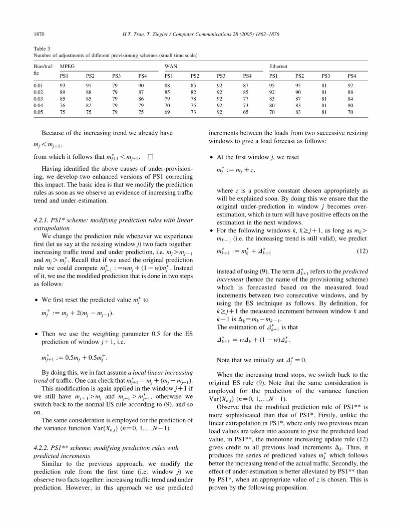
Table 3

Number of adjustments of different provisioning schemes (small time scale)

Bias/traf-

fic

MPEG WAN Ethernet

PS1 PS2 PS3 PS4 PS1 PS2 PS3 PS4 PS1 PS2 PS3 PS4

0.01 93 91 79 90 88 85 92 87 95 95 81 92

0.02 89 88 79 87 85 82 92 85 92 90 81 88

0.03 85 85 79 86 79 78 92 77 83 87 81 84

0.04 76 82 79 79 70 75 92 73 80 83 81 80

0.05 75 75 79 75 69 73 92 65 70 83 81 70


Because of the increasing trend we already have

mj!mjC1;

from which it follows that m�jC1!mjC1. ,

Having identified the above causes of under-provision-

ing, we develop two enhanced versions of PS1 correcting

this impact. The basic idea is that we modify the prediction

rules as soon as we observe an evidence of increasing traffic

trend and under-estimation.

4.2.1. PS1* scheme: modifying prediction rules with linear

extrapolation

We change the prediction rule whenever we experience

first (let us say at the resizing window j) two facts together:

increasing traffic trend and under prediction, i.e. mjOmjK1

and mjOm�j . Recall that if we used the original prediction

rule we could compute m�jC1 :ZwmjC ð1KwÞm�

j . Instead

of it, we use the modified prediction that is done in two steps

as follows:

†
We first reset the predicted value m�j to
mCj :Z mj C2ðmj KmjK1Þ:

†
Then we use the weighting parameter 0.5 for the ES
prediction of window jC1, i.e.

m�jC1 :Z 0:5mj C0:5mC

j :

By doing this, we in fact assume a local linear increasing

trend of traffic. One can check that m�jC1Zmj C ðmjKmjK1Þ.

This modification is again applied in the window jC1 if

we still have mjC1Omj and mjC1Om�jC1, otherwise we

switch back to the normal ES rule according to (9), and so

on.

The same consideration is employed for the prediction of

the variance function Var{Xn,j} (nZ0, 1,.,NK1).

4.2.2. PS1** scheme: modifying prediction rules with

predicted increments

Similar to the previous approach, we modify the

prediction rule from the first time (i.e. window j) we

observe two facts together: increasing traffic trend and under

prediction. However, in this approach we use predicted

increments between the loads from two successive resizing

windows to give a load forecast as follows:

†
At the first window j, we reset
m�j :Z mj Cz;

where z is a positive constant chosen appropriately as

will be explained soon. By doing this we ensure that the

original under-prediction in window j becomes over-

estimation, which in turn will have positive effects on the

estimation in the next windows.

†
For the following windows k, kRjC1, as long as mkOmkK1 (i.e. the increasing trend is still valid), we predict
m�kC1 :Z m�

k CD�kC1 (12)

instead of using (9). The term D�kC1 refers to the predicted

increment (hence the name of the provisioning scheme)

which is forecasted based on the measured load

increments between two consecutive windows, and by

using the ES technique as follows. By definition, for

kRjC1 the measured increment between window k and

kK1 is DkZmkKmkK1.

The estimation of D�kC1 is that

D�kC1 Z wDk C ð1 KwÞD�

k :

Note that we initially set D�j Z0.

When the increasing trend stops, we switch back to the

original ES rule (9). Note that the same consideration is

employed for the prediction of the variance function

Var{Xn,j} (nZ0, 1,.,NK1).

Observe that the modified prediction rule of PS1** is

more sophisticated than that of PS1*. Firstly, unlike the

linear extrapolation in PS1*, where only two previous mean

load values are taken into account to give the predicted load

value, in PS1**, the monotone increasing update rule (12)

gives credit to all previous load increments Dk. Thus, it

produces the series of predicted values m�k which follows

better the increasing trend of the actual traffic. Secondly, the

effect of under-estimation is better alleviated by PS1** than

by PS1*, when an appropriate value of z is chosen. This is

proven by the following proposition.

Fig. 8. Delay violation probability (MPEG traffic, small time scale).

Fig. 10. Delay violation probability (WAN traffic, small time scale).

Fig. 9. Delay violation probability (MPEG traffic, large time scale).

Fig. 11. Delay violation probability (WAN traffic, large time scale).

Fig. 12. Delay violation probability (Ethernet traffic, small time scale). Fig. 13. Delay violation probability (Ethernet traffic, large time scale).


Table 4

AGF values of PS1, PS2, PS1* and PS1** provisioning schemes


Scheme/traffic MPEG, uoptZ0.772 WAN, uoptZ0.890 Ethernet, uoptZ0.804 MPEG, uoptZ0.788 WAN, uoptZ0.781 Ethernet, uoptZ0.737

PS1 0.880 0.898 0.913 0.704 0.721 0.840

PS2 0.916 0.914 0.914 0.683 0.803 0.848

PS3 0.750 0.830 0.841 0.443 K0.133 0.794

PS4 0.889 0.908 0.912 0.556 0.503 0.676

PS1* 0.909 0.935 0.895 0.788 0.814 0.847

PS1** 0.883 0.915 0.870 0.739 0.847 0.855


Proposition 4.1. If z is chosen such that zO(1Kw)Dj,

whenever load under-estimation might happen, PS1**

performs better than PS1* in the sense that it produces a

smaller degree of under-estimation or does not under-

estimate at all.

Proof. See Appendix A.

4.3. Performance evaluation of the enhanced

provisioning schemes

We plot the delay violation probability as a function of

the delay bound in Figs. 8–13, which were obtained with

trace driven simulation for all the provisioning schemes we

have considered so far. The delay violation probability for

a given delay bound D is determined from the set of per-

packet delay samples collected in simulation according to

the formula:

PðdelayODÞ

ZNumber of delay samples with value bigger than D

Total number of delay samples:

In case of PS1** scheme, the specific delay bound

associated with the violation probability of 10K4 is

particularly marked in the figures.

The figures indeed demonstrate significant improvements

attainable with PS1* and PS1** schemes, ranking them to be

the best. The original target QoS P(delayO10 ms)!10K4 is

met closest by the PS1** scheme.3 Also note that the QoS

attained with simulation for the rest of schemes is worse

3 One can observe in Fig. 9 that in case of MPEG traffic, application of

large measurement slots leads to considerably worse QoS than the target

QoS. This is because the schemes assign the bandwidth calculated based on

large time scale (1200 ms) measurements, in which the smaller time scale

(40 ms) fluctuations are averaged out. In simulation, the traffic loads

measured in 40 ms slots, i.e. at a finer time granularity were used as the

input traffic. Consequently, the bandwidths allocated with regard only to

large time scale traffic dynamics fail to cope with small time scale traffic

fluctuations, resulting in worse QoS than the target QoS.

Our experiments have also indicated that measurement time slots with

length 40 ms prove to be a sufficient and reliable measurement granularity

applied in our provisioning schemes. Currently, we are working on the

consistent concept of the choice for the most proper measurement time

scale.

than the original QoS target, i.e. we only have

P(delayOD)!10K4 for such D value, which is significantly

larger than 10 ms. This QoS dissatisfaction is exactly due to

the effect of under-provisioning stemming from traffic under-

estimation during a certain number of windows which have

been investigated before in Section 4.2.

Table 4 reports the AGF values of all the provisioning

schemes. This is in fact Table 2 (presented earlier in Section

3.2) extended with the AGF values of schemes PS1* and

PS1**. Observe from Table 4 that in a major part of the

cases the PS1* and PS1** schemes have bigger AGF values

than other schemes, demonstrating their better goodness.

There remain some cases, when the obtained AGF values of

PS1* and PS1** scheme are slightly smaller than that of

PS1 and PS2 scheme. This is due to the degree of over-

dimensioning involved in PS1* and PS1** schemes at the

price of the QoS improvements. Note that in fact we do not

have extensive over-dimensioning. For example, in case of

the Ethernet traffic trace, the computed AGF values for

PS1* and PS1** are 0.895 and 0.870 in case of small time

scale provisioning, i.e. still in the range of the corresponding

AGFs of PS1 and PS2 (which is 0.91).

5. Potential applicability of the proposed provisioning

schemes

We briefly list in this section some typical scenarios, in

which the application of our provisioning is well con-

ceivable. The scenarios are namely (i) adaptive resizing of

high-speed LSPs (Label Switched Paths) in MPLS net-

works; (ii) adaptive resizing of customer-pipes in VPNs

(Virtual Private Networks); (iii) adaptive bandwidth

allocation of logical links in the Service Overlay Networks

architecture [1] for providing end-to-end QoS over inter

domains; (iv) and resizing of SLA between DiffServ

domains.

5.1. Resizing of LSPs in MPLS networks

In the context of MPLS technology, LSPs are considered

as tunnels accommodating the traffic over the MPLS

domain. By applying our provisioning schemes, for any

given tunnel the operator can adaptively resize the

allocated bandwidth in order to meet the required QoS of


the incoming traffic. The application will involve the

deployment of periodical traffic monitoring at the ingress

router of the LSP and the execution of our bandwidth

assignment scheme.

Note that signalling is required for bandwidth reassign-

ments. However, we can exploit the refresh messages in the

soft-state RSVP-TE [10], the current signalling protocol for

MPLS for this purpose.4 Thus, we do not need additional

signalling overhead compared to the current RSVP-TE

MPLS architecture to achieve QoS-aware adaptive

provisioning.

5.2. Resizing of customer pipes in VPN

(Virtual Private Networks)

Virtual Private Networks (VPN) is the concept of serving

a special group of customers (be they end users or

institutes). The service providers reserve bandwidths

between the end points to convey traffic demands.

The bandwidth is allocated using either pipe or hose

model [3]. In order to offer services competent with those of

networks of physical private lines, encryption and quality

guarantees are required to be delivered in VPNs. As long as

the pipe concept is followed, our proposed provisioning

schemes in fact provide an efficient solution for the

bandwidth management of the pipes, or in other words,

the virtual links.

Concerning the implementation issues, the same con-

siderations as in the LSPs case are valid. The concrete

signalling procedure to adapt the needed bandwidth depends

on the underlying technology of the given VPN. The

signalling protocol for example can be Beagle [11], or

RSVP. Note that the monitoring capability is required only

at the ingress router of the virtual link.

5.3. Resizing of SLA between DiffServ domains

One way for providing QoS over multiple network

domains is to deploy the DiffServ architecture in individual

network domains and employ peer-to-peer SLA (Service

Level Agreement) to control the traffic between neighboring

domains. Such SLAs specify the amount of traffic that can be

carried over the inter-domain link. Through this link, Virtual

Leased Lines (VLLs) can be established to ensure point-to-

point QoS. Our provisioning schemes apply to dynamic

resizing of such VLLs in order to meet the required QoS.

The signalling for bandwidth adjustments again is

resolved in a request-acknowledge manner involving edge

routers and an automated management entity like a

Bandwidth Broker (BB). The edge router of one domain

accomplishes traffic monitoring and initiates the bandwidth

adjustment request toward the BB. The BB processes

4 The default period between refreshing messages is 30 s but this value

can be configurable.

this request, carries out the re-assignment, updates its

databases if necessary, and sends back the acknowledge-

ment to the router.

5.4. Resizing of logical links in SON

(Service Overlay Networks)

Service Overlay Network (SON) is the alternative

concept for providing inter-domain end-to-end QoS [1].

SON is a network lying on the top of individual domains.

In SON, devices called service gateways are deployed in the

underlying domains and interconnected with logical links.

Each logical link is in fact a path comprising a series of IP

links in the underlying domains. The bandwidths of logical

links are purchased by SON from the underlying network

domains. By adaptively adjusting the bandwidth of the

logical links of the SON, efficient bandwidth management is

achievable which makes the SON deployment and operation

more profitable.

The traffic measurements have to be done at the service

gateways. This means that the monitoring capability should

be integrated into the software module of the gateways, as

similarly required for the ingress router in case of LSPs or

customer pipes of VPNs. In addition, signalling messages

must be exchanged between the gateways of the SON and

the routers of the underlying domains to declare and process

the bandwidth allocation and/or release requests. Note that

the application thus needs also the support of the underlying

networks.

6. Related work

There has been a large amount of work in the area of

adaptive bandwidth provisioning. Without the goal of

providing a complete survey, we briefly describe below

some recent provisioning schemes that share one or more

common aspects with our work.

Beyond the two already investigated schemes PS3 and

PS4 [1,3], [12] proposes a scheme to adaptively allocate the

bandwidth between bandwidth brokers of peer DiffServ

domains. This work has two common aspects with our work.

The first aspect is the aggregation nature of the accom-

modated traffic. The second aspect is the measurement-

based nature of the scheme, i.e. the aggregate traffic load is

collected in a timeslot-based manner and resizing is done in

a window-based manner. However, in spite of these

similarities, there are some major differences compared to

our schemes. Not only the specific techniques used in the

scheme of [12] (a discrete Kalman filter and a transient

analysis of a M/M/N queue) are different, but more

importantly is its special flow-oriented nature. In essence,

[12] assumes a priori fix and identical bandwidth require-

ment for each traffic flow. The bandwidth to be provisioned

thus is expressed in the number of flows. Because of the lack

of specifying how this per-flow bandwidth value could be


deduced from the packet level QoS, the scheme in [12]

cannot be directly used if the latter one is the target for

provisioning.

Ref. [13] is another recent work proposing a measure-

ment-based scheme for adaptive bandwidth allocation for

aggregate traffic. It advocates the use of Fractional Stable

Noise (i.e. the a-stable long-range dependent stochastic

process) as a model for the aggregate traffic. However, [13]

adopts this specific traffic model essentially only for having

an efficient linear traffic prediction, and not for the

derivation of mapping rules between QoS requirement and

bandwidth. The traffic prediction is namely based on the so

called minimum dispersion criterion, which relies in turn on

the properties of a-stable process. No explicit mapping

between packet level QoS requirements and bandwidth to be

provisioned is provided. Instead, the authors simply propose

to over-allocate the bandwidth with a certain over-allocating

factor. Consequently, in case packet level QoS requirements

are given as the target for provisioning, the scheme of [13]

can neither be directly applied.

Ref. [14] works out a provisioning scheme for VPN links

involving a specific traffic prediction called Linear Pre-

dictor with Dynamic Error Compensation (L-PREDEC).

The provisioning scheme uses the so called over-reservation

factor a to set the bandwidth to aserrCm, where serr is the

mean square error of the predictor, m is the measured mean

rate. However, this work does not provide any explicit

mapping between statistical QoS and bandwidth to be

provisioned. Again, if we are about to achieve a target

statistical QoS on packet delay, there is no means to choose

the right value of the over-provisioning factor a.

One of commercially available solutions for dynamic

bandwidth provisioning is the Cisco MPLS AutoBandwidth

allocator [15], where the local maximum approach is used.

The average traffic rate is sampled in each measurement

time slots. The bandwidth of a given MPLS tunnel is

adjusted after each configurable resizing interval compris-

ing a certain number of measurement time slots. The

bandwidth for the next resizing interval is set to the largest

average rate of the last interval. This provisioning scheme is

very simple, but may practically be inefficient due to the

lack of an explicit QoS-aware respect.

In summary, neither of the schemes available in [1,3,12–

15] is suitable for a direct use, when packet level statistical

QoS is considered as the explicit target for the provisioning

task. To our best knowledge, only the work from [16]

represents an alternative of our scheme. This work addresses

the same issue as ours, i.e. to provision a link given the

packet level delay violation probability as the target QoS

requirement. To relate this QoS requirement to the needed

bandwidth, [16] proposes to use the 2-scale Fractional

Brownian Motion traffic model. However, beside a different

traffic model, this work also differs from our work in several

points. The parameters of the traffic model are calculated

off-line from measurement data of traffic traces by means of

the technique of empirical linear regressions. Moreover,

unlike our solution, no sophisticated traffic prediction rules

are involved in the scheme of [16] to improve its

performance.

7. Conclusions

Our research was inspired by the fact that bandwidth

provisioning is done mostly in a utilization threshold based

manner. However, the role of the chosen utilization

threshold in QoS is often not tackled or even neglected

in previous research work. In contrast to this, we worked

out novel provisioning schemes that render the bandwidth

with explicit respect to the target QoS like packet delay

and packet loss ratio. We have first developed two novel

provisioning schemes called PS1 and PS2, incorporating

periodical measurements, predictions of traffic dynamics

and the Gaussian traffic model. Investigations based on our

trace driven simulation and on the AGF (Average

Goodness Factor) assessment have clearly shown the

advantage of the developed schemes compared to some

other existing ones.

Furthermore, the experiments with PS1 and PS2 schemes

have raised the need for further enhancement efforts

concerning signalling overhead reduction and avoidance

of under provisioning. Our efforts have resulted in two

improved versions of the PS1 scheme, to which we referred

to as the PS1* and PS1** schemes. Thorough investigations

confirm that these PS1* and PS1** schemes indeed perform

very well regarding both QoS achievement and economical

resource usage. As a summary, we conclude that

†
With our schemes, bandwidth is adaptively adjusted with
explicit regards to the live traffic dynamics and the target,

packet level statistical QoS. The bandwidth calculation

relies on a single binary search, which does not require

cumbersome computational efforts. Our schemes enables

efficient provisioning in the sense that they result in

neither excessive over-provisioning, nor severe under-

provisioning.

†
The proposed schemes bear a wide range of potential
applications. Whenever the aggregation degree of the

traffic is sufficiently high to justify the application of the

Gaussian model, and statistical QoS is desirable with

economical resource usage, the use of our schemes is

well grounded.

Some associated work items remain as topics requiring

further investigations. For example, we are currently

working on the insights into the effect of the length of

measurement time slots. We have stated earlier that the

proposed schemes work well with sufficiently fine granu-

larity of traffic load measurement, which for example is in

range of 40 ms. A rigorous concept of choosing the most

proper measurement granularity is the goal of our current

research.

Table A1

The number of windows where the prediction rule must be changed and

among them the number of those, where zZm�jK1 KmjK1 O ð1KwÞDj is

held

MPEG WAN Ethernet

Changed-windows 28 31 20


Acknowledgements

This work has been partly supported by the Austrian

government’s Kplus Competence Center Program, and by

the European Union under the E-Next Project

FP6-506869.
Proper-windows 15 16 17
Appendix A. Proof of Proposition 4.1

The proposition states that:

If z is chosen such that zO(1Kw)Dj, whenever load

under-estimation might happen, PS1** performs

better than PS1* in the sense that it produces a smaller

degree of under-estimation or does not underestimate

at all.

Proof. For clarity, we will add to the subindex of m* the

term PS1* or PS1** to indicate the scheme being applied to

get this predicted value.

Recall that the original prediction rule is changed in

window j. Keeping it in mind, we have the following

relation:

m�jC1;PS1�� Z m�

j;PS1�� CD�jC1

Z mj Cz CwDj C ð1 KwÞD�j

Z mj Cz CwDj ðremember that D�j is set to 0Þ

Omj CDj

Z mj C ðmj KmjK1Þ Z m�jC1;PS1�

(A1)

The above inequality is valid if we choose an appropriate

z, such that zO(1Kw)Dj. The inequality (A1) basically

means that if the traffic dynamics is such that changing the

prediction rule in window j according to PS1* scheme still

leads to under-estimation in widow jC1, then applying the

prediction rule of PS1** scheme surely brings either

smaller under-estimation or does not produce under-

estimation at all.

Now, let us consider the case when under-estimation

occurs again in window jCl(lO1), after the modified rule

has been applied in window j. We will show that using

PS1** scheme (i.e. applying the rule (12) from window j)

yields better performance than using PS1* scheme (i.e.

applying linear extrapolation in window j, and then the

normal ES technique (9) from window jC1 until window

jClK1).

Since from window j to window jCl, under-estimation

does not occur, the ES technique (9) is applied in PS1*

scheme from window jC1 until window jClK1. Thus, we

have

m�jC1;PS1� Z wmjClK1 C ð1 KwÞm�

jClK1;PS1�

!maxðm�jClK1;PS1� ;mjClK1Þ

Z m�jClK1;PS1� :

Recursively applying the above argument, it follows that

m�jCl;PS1� !m�

jClK1;PS1� !/!m�jC1;PS1� . Thus, because of the

inequality (A1) we arrive at


jC1;PS1�� (A2)

On the other hand, if PS1** scheme is applied from

window j, then due to rule (12) we have

m�jCl;PS1�� !m�

jC2;PS1�� !/!m�jCl;PS1�� (A3)

Combining (A2) and (A3) follows that


jCl;PS1�� ; (A4)

and this completes our proof. ,

Remark. In the analysis reported in the paper, we set

zZm�jK1KmjK1. With our specific traffic traces, we have

checked and seen that more than 50% of the cases when we

have to modify the prediction rule, the condition zZm�jC1K

mjK1O ð1KwÞDj is held. More precisely, over a period of

100 resizing windows, Table A1 shows the number of

windows in which we have to change the prediction rule

(referred to as changed-windows) and among them the

number of windows in which the above mentioned

inequality is true (proper-windows).

Despite that zO(1Kw)Dj is not always true, we obtain

fairly good results with PS1** scheme, which are still better

than those of PS1* scheme. This was demonstrated in

Section 4.3.

References

[1] Z. Duan, Z.-L. Zhang, Y.T. Hou. Service overlay networks: SLAs,

QoS and bandwidth provisioning, in: Proceedings of IEEE 10th

International Conference on Network Protocols (ICNP), 2002, pp.

334–343.

[2] K. Papagiannaki, N. Taft, Z.-L. Zhang, C. Diot. Long-term forecasting

of internet backbone traffic: observations and initial models, in:

Proceedings of IEEE INFOCOM, vol. 2, 2003, pp. 1178–1188.

[3] N.G. Duffield, P. Goyal, A. Greenberg. A flexible model for resource

management in virtual private networks, in: Proceedings of

SIGCOMM, 1999, pp. 95–108.


[4] R.G. Addie, M. Zukerman, T.D. Neame, Broadband traffic modeling:

simple solution to hard problem, IEEE Communications Magazine 36

(8) (1998) 88–95.

[5] J. Choe, N.B. Shroff, A central limit theorem based approach for

analyzing queue behavior in high speed networks, IEEE/ACM

Transactions on Networking 6 (5) (1998) 659–671.

[6] H.S. Kim, N.B. Shroff, Loss probability calculations and asymptotic

analysis for finite buffer multiplexers, IEEE/ACM Transactions on

Networking 9 (6) (2001) 755–768.

[7] W.S. Wei, Time Series Analysis, Addison-Wesley, 1990.

[8] MPEG traces. ftp-info3.informatik.uni-wuerzburg.de/pub/MPEG/

[9] The Internet traffic archive. http://ita.ee.lbl.gov/index.html

[10] D. Awduche, L. Berger, D. Gan, T. Li, V. Srinivasan, G. Swallow. RSVP-

TE: Extensions to RSVP for LSP Tunnels. RFC3209, December 2001.

[11] L.K. Lim, J. Gao, T.S. Eugene Ng, P.R. Chandra, P. Steenkiste,

H. Zhang, Customizable virtual private network service with QoS,

Computer Networks 36 (2001) 137–151.

[12] T. Anjali, C. Scoglio, G. Uhl, A new scheme for traffic estimation and

resource allocation for bandwidth brokers, Computer Networks 41 (6)

(2003) 761–777.

[13] M. Lopez-Guerrero, J.R. Gallardo, L. Orozco-Barbosa, D. Makrakis,

On the linear prediction of aggregate network traffic and its

application to dynamic resource management, Computer Communi-

cations 26 (12) (2003) 1341–1352.

[14] W. Cui, M.A. Bassiouni, Virtual private network bandwidth manage-

ment with traffic prediction, Computer Networks 42 (6) (2003)

765–778.

[15] Cisco MPLS AutoBandwidth Allocator for MPLS traffic

Engineering: A Unique New Feature of Cisco IOS

Software. http://www.cisco.com/warp/public/cc/pd/iosw/prodlit/

mpatbwp.htm

[16] C. Fraleigh, F. Tobagi, C. Diot. Provisioning IP backbone networks to

support latency sensitive traffic, in: Proceedings of INFOCOM, vol. 1,

2003, pp. 375–385.

http://ftp-info3.informatik.uni-wuerzburg.de/pub/MPEG/

http://ita.ee.lbl.gov/index.html

http://www.cisco.com/warp/public/cc/pd/iosw/prodlit/mpatbwp.htm

http://www.cisco.com/warp/public/cc/pd/iosw/prodlit/mpatbwp.htm

Adaptive bandwidth provisioning with explicit respect to QoS requirements

Documents

Transcript of Adaptive bandwidth provisioning with explicit respect to QoS requirements