active vibration control of composite structures - VTechWorks

ACTIVE VIBRATION CONTROL OF COMPOSITE STRUCTURES

by

Min- Yung Chang

Dissertation submitted to the Faculty of the

Virginia Polytechnic Institute and State University

in partial fulfillment of the requirements for the degree of

DOCTOR OF PHILOSOPHY

in

Engineering Mechanics

We

Nand ee

a,

M. S. Cramer cael Frederick

La. heca0inrKkl Lute

L. Meirovitch Ss R. H. Plaut

July, 1990

Blacksburg, Virginia

ACTIVE VIBRATION CONTROL OF COMPOSITE STRUCTURES

by

Min- Yung Chang

L. Librescu Chairman

Engineering Mechanics

(ABSTRACT)

The vibration control of composite beams and plates subjected to a travelling load

is studied in this dissertation. By comparing the controlled as well as uncontrolled re-

sponses of classical and refined structural models, the influence of several important

composite structure properties which are not included in the classical structural model

is revealed.

The modal control approach is employed to suppress the structural vibration. In

modal control, the control is effected by controlling the modes of the system. The con-

trol law is obtained by using the optimal control theory. Comparison of two variants

of the modal control approach, the coupled modal control (CMC) and independent

modal-space control (IMSC), is made. The results are found to be in agreement with

those obtained by previous investigators. The differences between the controlled re-

sponses as well as actuator outputs that are predicted by the classical and the refined

structural models are outlined in this work.

In conclusion, it is found that, when performing the structural analysis and control

system design for a composite structure, the classical structural models (such as the

Euler-Bernoulli beam and Kirchhoff plate) yield erroneous conclusions concerning the

performance of the actual structural system. Furthermore, transverse shear deforma-

tion, anisotropy, damping, and the parameters associated with the travelling load are

shown to have great influence on the controlled as well as uncontrolled responses of the

composite structure.

Acknowledgements

I wish to express my sincere gratitude to Dr. Liviu Librescu as my advisor and

teacher. From him, I have acquired much knowledge and insight into the modelling and

analysis of composite structures. His enthusiasm and direction have proved to be in-

valuable.

I would also like to thank Dr. M. S. Cramer, Dr. D. Frederick, Dr. L. Meirovitch,

Dr. R. H. Plaut, and Dr. J. N. Reddy for serving as members of my committee. I have

benefited very much from the courses that I have taken from them. Also, I would like

to add a special thanks to Dr. Meirovitch for providing me a thorough and complete

understanding of the important concepts in the control of structures.

I am indebted to Dr. Plaut for his time and effort to read the dissertation and make

many useful suggestions, and to Mr. Michael Smith, a fellow graduate student of the

ESM department, for providing some grammatical editing suggestions throughout the

text.

Additionally, I wish to acknowledge the partial financial support which I have re-

ceived from the ESM department as a graduate teaching assistant during my years at

Virginia Tech.

Acknowledgements iii

I would also like to thank my parents, brothers, and sister for their understandings

and unending support.

Finally, I would like to thank my wife Li-Jane for her patience and sacrifice through

these years, and my lovely daughter Jenny for providing me so much joy and comfort.

Acknowledgements iv

Table of Contents

Chapter 1 Introduction 2.0... . ccc cc cece eee ee ee eee eee eee eee eee eee ee eee eees 1

1.1 Background 2.0... . cece eee tenet eee ete eee ene e eens 1

1.2 Problem Description ......... cece cee cee ee ee ee eee eee eee eee e eens 5

Chapter 2 Governing Equations of Elastic Structures 2.2.0... . cee cece eee ee tees 9

2.1 Introduction 2.2... .... ccc ee ce ee ee ee eee eee eee eee eee eee 9

2.2 Equations of Motion of 3D Linear Elastic Bodies ......... 0... 0... cece ee eee 11

2.3 Governing Equations of Plates and Beams .. 1... .. cee cc ee nee ee tees 13

2.3.1 Introduction 2.0... ... cece ee eee ee eee ee eee ee ne ene 13

2.3.2 Displacements and Strains ..... 0... cee ec ee ee teen e eee eens 14

2.3.3 Stresses and Constitutive Relations ......... 2.0... cece eee ee eee eee eens 16

2.3.4 Two-Dimensional Equations of Motion ....... 0... . 0... eee ee eee ee ee eens 19

2.3.5 Governing Equations ....... cee cece eee eee eee eens 21

2.4 Direct Derivation of the Governing Equation of SLB .... 1... ee ee ee eee eee 31

Chapter 3 Eigensolutions and Uncontrolled Dynamic Responses ............. eee eeeees 36

3.1L Introduction 2.0... . ccc cc eee ee eee eee eet ee eee ee eee ee ee eee eee 36

Table of Contents Vv

3.2 Eigensolutions of Beams... 1... ee ec eee ete et ee tenet e eee aes 37

3.3 Dynamic Response of Beams ........ 0... cece eee eee ete ete eet e eens 43

3.4 Eigensolutions of Plates 20... cee ee ee nent e eee ees 55

3.5 Another Method of Finding Eigenfrequenckhs .......... 2... eee cee eee eee 63

3.6 Dynamic Response of Plates 2.0... . ee ec tee eee teen e eee 66

Chapter 4 Control System Design ........ ccc cc ccc cee eee eee ree erence eee eeese 74

4.1 Introduction . 0... ee tee eee eee eee nent eens 74

4.2 Linear Optimal Regulator 2.1... . eee ee te ete e ete eee nee 76

4.3 The Vibration Control of Beams «1... tee eee ene 85

4.3.1 Coupled Modal Control (CMC) ...... 0... cece ee ee ee ee enna 87

4.3.2 Independent Modal-Space Control (IMSC) ........ 0... . cece eee ee eee 89

4.3.3 Controlled Dynamic Response of Beams ... occ bee e eee e eens eennneeg 91

4.4 The Vibration Control of Plates 0... 0... ce ce ce eee tenet nee 96

Chapter 5 Results and Discussion ........ 0c csc cece ec cece cece r etree eee ee eeeses 99

5.1 Beams without Control 2... .... cee ee ee eee tt ete eee 104

S.1.1 Eigenfrequencies 2.0... cee eee ee ee tet eee eee eee eee 104

5.1.2 Uncontrolled Dynamic Response .......... 0... ccc cee ee teen e eee 115

5.2 Plates without Control 2.0... 2... eee eee tent e teens 131

5.2.1 Eigenfrequencies 2.0... cee ee ee eee eee eee ee eee ees 131

5.2.2 Uncontrolled Dynamic Response .......... 0... eee eee eee eee eee ees 131

5.3 Beams with Control 2.0... . ccc ee ete ee eee tee ene t ene 157

5.3.1 Closed-Loop Poles 2.1... ... ec cc cc eet ee eee eee e eens 157

5.3.2 Controlled Dynamic Response ............ 0. cece eee eee eee tee eens 172

5.3.3 Performance Index, Cost Kernel and Actuator Output ..................00.4. 196

5.4 Plates with Control 2.2... ce ne eee ee eee ee nee ete e eens 212

5.4.1 Controlled Dynamic Response ........... 0. cece eee eee eee teens 212

Table of Contents vi

5.4.2 Cost Kernel .... 0... ccc ce ee eee ee ee eee eee eee eee eee ee eee ees 224

5.4.3 Actuators’ Output 2.0... ce ee eee ete eee ee nen 238

Chapter 6 Conclusion and Recommendations .......... 00sec eee r cece see eeeees 249

Appendix Al: Nondimensional Form of the Governing Equation of Beams ............. 252

Appendix A2: Determining the Positiveness of an Expression ........... sce eeeeenes 255

Appendix A3: Derivation of Modal Equations ............ cee ec cere cece ene eenes 260

Appendix A4: Dimensionless Form of the Governing Equation of Plates .............. 266

Appendix B1: The Integral Solution Form of Linear Systems ......... 0.0.0 sec eeeees 269

REFERENCES 2... ccc cc ec ce eter eee reer eee eee teens 272

Table of Contents vii

Chapter | Introduction

1.1 Background

A great deal of theoretical and experimental work has been carried out in the area

of active structural vibration control in recent years (see, e.g., [1-23]). A good source

of information related to this problem can be found in text books [24,25] and review

articles [26,27]. These studies have revealed that the structural vibration can be sup-

pressed very effectively by means of the active control technique. The type of control

generally used is the feedback control whereby control forces and torques, which are

related to the displacements and velocities of the structure, are applied to the structure

in order to produce a desired response. Physically, these control inputs provide addi-

tional stiffness and damping to the controlled structure. In contrast to the passive vi-

bration control methods (i.e., shock absorbers, viscous dampers and damping layers

[28]), the active control approach provides a more effective way of controlling the

structural response. Active control is more versatile; control gains can be adjusted so

as to satisfy various performance criteria. Moreover, active control can improve the

Chapter | Introduction 1

structural response over a much broader frequency range; passive control is severely

limited to a narrow band. These desirable features, to name a few, make active control

very attractive to be used in controlling the response of a structure.

Quite often, in engineering applications, the structure’s vibration must be contained

within an admissible level or be suppressed totally. For example, controlling the vi-

bration of the structure is required:

e to reduce the large vibrational motion of structures that induces high local stresses

which may exceed the structure’s strength limit,

e to quickly suppress the slowly decaying vibration that is characteristic of a lightly

damped and/or highly flexible structure,

¢ to remove the unstable structural motion that may occur when nonconservative

forces are present (for example, flutter in the presence of aerodynamic and follower

forces) {29,30},

e to eliminate the disturbance in a system caused by the vibration of its supporting

structure; this is especially crucial for the system when a high precision is required,

e to reduce the level of noise induced by the structural vibration [31].

With the advent of the newly developed advanced composite materials such as

fiber-reinforced composites, new structural analysis techniques and design methods have

to be adopted. The use of the composite materials in modern engineering applications

(e.g., aeronautical vehicles, marine structures, space structures, robotics) is increasing

because composite materials provide many desirable properties. Among these are re-

sistance to chemical action, high fatigue resistance, high strength/rigidity in relation to

weight [32,33]. However, the composite material structures are generally heterogeneous,

anisotropic, and have high flexibility in transverse shear. It has been shown previously


[33-48] that the classical structural model, which is based on the theories such as

Bernoulli-Euler (beams), Kirchhoff (plates) [49] (which are also known as the classical

theory (CT)), may no longer adequately represent this type of structure. One impli-

cation of using the CT is that the structural member is assumed to possess an infinite

transverse shear rigidity, which contradicts the real properties that the composite struc-

ture exhibits.

Improvements of the classical structural model have been made by many research-

ers. Among the earlier contributors, one can cite, for example, Reissner [50] and Mindlin

[51] for plates, and Timoshenko [52] for beams. These authors incorporated the trans-

verse shear deformation effect in the structural model, while the latter two authors ad-

ditionally considered in their respective models the dynamic terms accounting for the

rotatory inertia effect. These structural theories are often referred to as the first-order

shear deformation theory (FOT).

Using the the structural model based on the FOT, better results of structural re-

sponses that were poorly predicted by its classical counterpart were obtained [36].

However, in some instances (e.g., the determination of transverse shear strains and

stresses), the FOT failed to yield satisfactory results [39,43-45]. This can be attributed

to the fact that there is only a first-order correction in the representation of in-plane

displacement fields in the FOT. As a result, it yields a uniform distribution of transverse

shear strains and stresses throughout the thickness of the structure (these quantities are

zero in the structural model based on the CT and can be recovered only through the use

of the three-dimensional stress equilibrium equations). However, a more accurate

characterization of these strain and stress components is that they vary parabolically

throughout the thickness of the structure. Because of such a discrepancy, shear cor-

rection factors [53] were introduced in the FOT model. The determination of shear

correction factors, however, becomes much more intricate for laminated composite


structures [54]. The requirement of using shear correction factors can be eliminated by

using the structural model based on the HOT.

In recent years, various higher-order refined theories (HOT) for structural modeling

have been developed (see [35,55-63] and the references contained therein). A great deal

of improvement in the prediction of the structural response has been achieved through

the use of the HOT, as opposed to that obtained from its FOT counterpart. Among

various HOTs, the one proposed by Librescu, Reddy [35,56,59] has certain advantages.

This theory incorporates the transverse shear deformation, transverse normal stress,

rotatory inertia as well as higher-order effects, while it yields a set of governing equations

having the same unknowns as the FOT. This feature arises from the stipulation of the

third-order in-plane displacement fields and the satisfaction of static boundary condi-

tions on the bounding planes. In this way, not only are governing equations expressed

in terms of a smaller number of dependent variables (same as those of the FOT) when

comparing with other HOTs, but also the transverse shear strain and stress components

exhibit parabolic distributions throughout the thickness of the structure. In view of the

latter property, there is no need for one to introduce the shear correction factors in this

theory. It has been shown [43-45] that the response of composite structures can be

predicted very accurately by using this higher-order theory.

With respect to response of a composite material structure, many previous studies

[33-48] showed that transverse shear deformation, as well as anisotropy and

heterogeneity, significantly influence the structural response. However, their effects on

the dynamic response of the composite structure which 1s actively controlled have not

been fully investigated. It is the goal of this study to obtain some important information

concerning the active vibration control of these new advanced composite structures.


1.2 Problem Description

Active control of the vibration of the structures made of advanced composite ma-

terials is the main subject of this research. A review of previous literature on this subject

indicates that most studies concerning the structural vibration control are restricted to

the cases involving conventional metallic structures. Work of limited scope has been

done in connection to the active vibration suppression of the composite structure [64,65].

The structural members investigated previously are only modelled within the framework

of the classical theory (CT), such as Bernoulli-Euler (beams) and Kirchhoff (plates)

theories. There are, however, a few vibration control-related studies that have been done

using a more accurate structural model [9,66-68]. But, the problem treated in these pa-

pers is only concerned with the isotropic structure modelled by the FOT, and there is

no attempt to make comparisons between the refined and classical models.

It is known that the structural model based on the CT adequately represents thin,

ordinary, metallic structures. However, it is inadequate for structures which are relatively

thick and/or are made up of new composite materials. Since composite structures ex-

hibit exotic properties, such as high degree of anisotropy and high flexibility in trans-

verse shear, a more refined structural model should be utilized. For the same reason,

when one is interested in the control of the vibration of the composite structure, using

a more accurate structural model could be crucial to predicting the performance of the

actually controlled system. Hence, one may expect that if the controller, which is used

to suppress the vibration of the structure, is designed based on the classical structural

model, one could obtain results which might not be reliable. It is the main focus of this

thesis to study such a problem. To state the problem differently, one may ask, “how is


the controlled response associated with the composite structure affected by the model-

ling error resulting from the use of the classical structural model ?”

One type of material that is of particular interest to the designer of aerospace vehi-

cles is pyrolitic graphite [69]. This material, which can be regarded as a transversely

isotropic material, has quite unusual properties. These include the high in-plane

Young’s to transverse shear moduli ratio (ranging from 20 to 50 or even higher in the

presence of a high temperature field), the increase of the strength to density ratio as the

temperature rises, and the thermal conductivity coefficient in the isotropic plane which

is many times greater than that in the planes normal to the isotropic plane (the ratio of

these coefficients ranges from 50 to 100) [33,69-72]. Such unusual properties render the

pyrolitic graphite type materials ideal to be used for the thermal protection of aerospace

vehicles.

The response of the structure made of pyrolitic graphite or, more generally, a

transversely isotropic material, was studied by Vinson, et al. [33,70-73], Librescu [35],

Ambartsumian [34], Brunelle [74-78], Chen and Doong [79]. In this thesis, the active

vibration control of a structure which is made of transversely isotropic materials sub-

jected to a travelling load is studied. Specifically, the following four types of structural

members will be considered:

1. single-layered transversely isotropic beams (SLB)

2. multilayered transversely isotropic beams (MLB)

3. single-layered transversely isotropic plates (SLP)

4. multilayered transversely isotropic plates (MLP)

There are various approaches to controlling the vibration of structures. One ap-

proach is modal control, whereby control of the structure is accomplished by controlling


its modes of vibration. For undamped structures, all the open-loop eigenvalues, gener-

ally known as poles, lie on the imaginary axis in the complex plane. In using the modal

control, the objective is to generate such feedback control forces and/or torques that

closed-loop poles will lie in the left half of the complex plane, thus causing the motion

of the structure to become asymptotically stable. Within modal control, one can dis-

tinguish between the case in which the design of the feedback forces is carried out for

all the controlled modes simultaneously [4] and the case in which the design is done for

each of the controlled modes independently [1,2]. The first case will be referred to as the

coupled modal control (CMC), while the second one proposed by Meirovitch [1,2] is

known as the independent modal-space control (IMSC). Both the CMC and IMSC

approaches will be considered in this study.

It is known [84,85] that the distributed structure, such as beams and plates, pos-

sesses an infinite number of modes. Although ideally one should control all these modes

to achieve the best control result, such a scheme may be impractical and/or too com-

plicated to be implemented. Since the dynamic response of structures is generally dom-

inated by lower modes and/or certain critical modes that tend to be destabilized, it is

adequate to control only these few modes. As a result, the structural vibration could

be effectively suppressed by using only a finite number of discrete-type force or torque

actuators.

The problem addressed in this dissertation is formulated and considered in the fol-

lowing way. In Chapter 2, the derivation of governing equations of the composite

beams and plates described earlier based on the higher order theory of Librescu and

Reddy [59] is presented. In these structural models, the transverse shear deformation,

transverse normal stress, rotatory inertia, as well as higher-order effects, are included.

In Chapter 3, eigensolutions (i.e., eigenfrequencies and eigenfunctions) are obtained by

solving the eigenvalue problem. Then, the uncontrolled dynamic response of structures

Chapter ! Introduction 7

is derived utilizing the modal analysis {84]. In Chapter 4, the system models derived from

modal equations for both CMC and IMSC approaches are described. Then, the vi-

bration suppression controller is designed using the linear optimal control theory [89,90].

The use of such a controller to control the structural vibration driven by a certain tran-

sient dynamic load is then analyzed.

In Chapter 5, several numerical examples are studied and their results are discussed.

All of the numerical results and simulations are carried out for structural members with

simply supported boundary conditions. In the first part of this chapter, the

eigenfrequencies as well as the uncontrolled dynamic responses of the structural models

based on the CT, FOT and HOT are analyzed and compared. In the second half, the

results of the vibration control of structures are given. In numerical examples, first, the

controller is designed for the structural model based on the CT (which will be referred

to as the nominal plant). Then, this controller is applied to the nominal plant as well

as the more accurate structural model based on the FOT or HOT (which will be called

the actual plant). Within this context, the modelling error and the influence of the pa-

rameters of the actual plant which may be uncertain or are subject to change are studied.

The results are then presented in the form of closed-loop pole locations, controlled vs.

uncontrolled responses, and some performance measures. Chapter 6 concludes this work

with some important conclusions on the present study and with recommendations for

future research.


Chapter 2 Governing Equations of Elastic Structures

2.1 Introduction

The structural member encountered in engineering applications often has the feature

that one or two of its geometric dimensions, for example the thickness, are much smaller

than the others. To analyze this type of structure, one might model them as one-

dimensional (1D) structural members using the beam theory, or as two-dimensional (2D)

structural members using the plate or shell theory. The advantage of using such models

is that the original three-dimensional (3D) problem is reduced to the corresponding 1D

or 2D one. Apparently, by considering the 1D or 2D model, the amount of work in-

volved in analysis is greatly reduced. In contrast, it might require an insurmountable

amount of work to analyze the structural member when it is treated as a three-

dimensional solid body.

It should be noted, however, that the structural model based on beam, plate, or shell

theory is only an approximate one (in the sense that it is an approximation of that de-

scribed by the three-dimensional theory). The accuracy of the solution predicted by us-

Chapter 2 Governing Equations of Elastic Structures 9

ing these models, hence, depends very much upon the assumptions being adopted in

each model. It is aimed at improving the accuracy of the solution predicted by these 1D

and 2D structural models that various refined beam, plate, and shell theories were de-

veloped. The previous theories are improved, for example, by removing some of the re-

strictions in the theory (such as Kirchhoff assumptions) and/or by considering a more

accurate representation of field variables (such as displacements and stresses).

The use of the refined theory, however, could result in the increase of the number

as well as of the order of governing equations. As a result, it would require more effort

to solve the problem than the case that uses the classical structural model. In view of

these facts, it seems important that one makes a judicious choice of the refined model

used in the analysis. One guideline for such a selection may be that with any chosen

refined structural model, the problem should remain manageable and, more importantly,

the structural responses of major concern that are determined should be accurate. For

example, when the interlaminar stresses are of major interest (as in the study of the de-

lamination problem of laminated composites), the selected refined model should be such

that the condition of continuity of displacements as well as of interlaminar stresses are

satisfied. However, in the case that only gross responses, such as displacements and

frequencies, are of major concern, the use of the more-complicated refined model might

not be justified. The reason for this is that some factors considered in the refinements

of the structural model might only have a very small influence on gross responses, while ~

the number and order of governing equations due to the inclusion of such factors are

increased greatly. Another important factor which should also be considered is that the

design and implementation of control systems could be hampered by the high order of

the system model. This will be discussed in a later chapter.

In the next section, the derivation of the stress equations of motion for three-

dimensional linear elastic bodies using Hamilton’s principle is considered. This is then


followed by the derivation of the governing equations of plates and beams using the

obtained 3D stress equations of motions.

2.2 Equations of Motion of 3D Linear Elastic Bodies

According to Hamulton’s principle, the stress equations of motion and associated

boundary conditions of 3D linear elastic bodies can be obtained from the following

variational equation [35]:

t

5I= | | | a! Sede — 5K - | slSVdA -| pB's vas | dt (2.2.1) L*t A, t

where K is the kinetic energy and is given by

k=4] oV,Wde (2.2.16) t

Various symbols and variables used in Eqs. (2.2.1) are defined as follows:

V = Vig, the displacement vector which is expressed in terms of the space

covariant base vectors of the undeformed body gz,

p mass density,

B= Big, the body force vector per unit mass of the undeformed body,

s=oin the components of the stress vector acting on the undeformed body,

a, e,, the components of the stress and strain tensor, respectively,


n, the components of the outward unit normal vector,

s' the components of s‘ prescribed on the part of A, of the boundary,

A, the remaining part of the boundary on which the displacement vector

V is prescribed,

6 the variation operator,

ly ty two arbitrary instants of time ¢ at which 6V, vanish.

It is known that if the elastic body is subjected to only small deformation, the strain

and displacement could be assumed to have the following linear relation:

ey = Vil) + Vil (2.2.2)

where the symbol (_ )||, denotes the space covariant derivative.

By considering the symmetry property of the stress tensor, applying the divergence

theorem, as well as performing the integration by parts, it was shown [35] that the vari-

ational equation, Eq. (2.2.1a), could be expressed as

61 = 61, + 61, =0 (2.2.3a)

where

61, = | i | [ol + o(B — V)J5 Vas | dt (2.2.36) & | “t

51, = inl Je — §)6 va | dt (2.2.3c)

According to Eqs. (2.2.3), the equations of motions and boundary conditions for linear

elastic bodies are given by


o'||, + p(B — VV) =0 (2.2.4)

if nol=s'=s' atA (2.2.4b) o

6Vi=0 at A, (2.2.4c)

Equations (2.2.4a) will be used in the derivation of the governing equations of plates and

beams shown in the next section.

2.3 Governing Equations of Plates and Beams

2.3.1 Introduction

The governing equations for the bending of symmetrically laminated plates were

obtained by Librescu and Reddy [59] based on a higher-order displacement field theory.

The emphasis of the word “displacement” is due to the fact that the theory is based on

the stipulation of a specific form of displacement fields. The other field variables such

as strains and stresses are then determined by using the kinematic and constitutive re-

lations. There are other structural theories such as the one proposed by Ambartsumian

[34] and by Reissner [50] where part of the displacement field as well as of the stress field

are postulated in the theory. For the comparison of various plate theories, see for ex-

ample [80].

According to the higher-order displacement field theory described in [59], for struc-

tural members such as plates and shells, the 3D displacement field variables could be


expanded in Taylor series form in terms of the thickness coordinate. The coefficients

of the series are the new unknowns (not depending on the thickness coordinate) to be

determined. Although there are an infinite number of terms in the Taylor series, in

practice only the first few terms in the series should be considered. The reason for this

is that the cost and effort of finding the solution of a problem increase tremendously as

more terms in the series are considered, and it is known from the asymptotic analysis

that since the thickness coordinate within the shell and plate has a relatively small value

(less than the thickness), the higher-order terms in the series generally have a smaller

effect on the solution.

Depending on the number of terms retained in the series, various higher-order dis-

placement field theories result [59-63]. In the following, the derivation of the governing

equations of symmetrically laminated plates based on a third-order displacement field

theory developed in [59] is reviewed.

2.3.2 Displacements and Strains

Since only the bending of plates is of interest here, according to the HOT described

in [59], the 3D displacement field could be expressed in terms of the thickness coordinate

x, as follows:

(1) (3) V(Xes X3p 0) = Xz Vg X yp 1) + (23) Ve(Xey D) (2.3.1a)

(0)

V3(Xu» X3y t) = V3(Xes t) (2.3.15)

where V, are the in-plane displacements and V, the transverse displacement.


It should be noted that here x, (i= 1, 2, 3) are the normal curvilinear coordinates,

in which x, (a = I, 2) denote the in-plane coordinates and x, the coordinate normal to

the plane x, = 0 (mid-plane of plates). Also, the Greek indices have values ranging from

1 to 2, while the Latin indices have values ranging from | to 3.

Due to the use of the normal curvilinear system of coordinates, for plates the fol-

lowing relations hold for metric tensors:

Exp = AaB, 823 = 943, 833 = 433 = 1 (2.3.2)

where g,, and a,, denote the components of the space and surface metric tensors, re-

spectively. Furthermore, there is no distinction between the space and surface differen-

tiations as well as between the covariant and contravariant components of a tensor.

The 3D strain components associated with the displacement field described by Eqs.

(2.3.1), according to Eq. (2.2.2), can be expressed as

(1) 3) Cup = X37 + (x4) erg (2.3.3a)

(0) 2) C3 =e + (x,)"2, (2.3.35)

€33 = 0 (2.3.3c)

ag 6 @ @ . . WheTe @,5, 29s C3» 243 are 2D strain components and are described by

My pO @ xp => (Vain + Mata) (2.3.4a)

(3) 1 (3) (3) exp => (Vaig + Vela) (2.3.4b)

(0) 1 (1) = (0) e3 = (Y, + Vs.) (2.3.4c)


@ 8) €43 = 3 Vi, (2.3.4a)

The single vertical stroke separating indices denotes the surface covariant derivative

2.3.3 Stresses and Constitutive Relations

Consider the case of the symmetrically laminated composite plate consisting of

2m + 1 uniform layers of anisotropic homogeneous materials (see Fig. 1). Furthermore,

assume that the material exhibits elastic symmetry with respect to the plane x, = con-

stant (i.e., the material is monoclinic). In this case, the generalized Hooke’s law for each

layer can be expressed as [35]

~ 33 oe = Ferre e. + Ee" oF

gp 3333

a | (03 ) 633 = F333 g op

where

~ 133 73348 ap _ pwnop _ ESSE

Eo = ~~ 73333

Chapter 2 Governing Equations of Elastic Structures

(2.3.5a)

(2.3.56)

(2.3.5c)

(2.3.5d)

16

ICU MAIS

Jt] JO

UOTZIAS SsotZ

“| aINsIy

(1 +z) |

(wz)

aue|d-piyy 4

I-wty reety

— =

Ox

itey \

(Z +

ut) ty

a

_-

ma

- ~~

(p+) |

| |

| “Yy

(uz) |

' ty

y

z i

{ i+ey

~-

zy ="y Z

|

(7)

()——}—"on

sadey

fy |

17 lastic Structures ~

“ Chapter 2 Governing Equations of F

Suppose that there are no shearing stresses and shear stress couples acting on the

bounding planes, Le.,

0 =0 at xy=tt 5 (2.3.6a)

[x30 ef. =0 (2.3.65)

where A denotes the total thickness of the laminate. Then, by making use of Eqs.

(2.3.3b), (2.3.4c-d), (2.3.5c) and (2.3.6), it can be shown that

(3) 4 ( (1) V = bu 5 (Yaat V;,) (2.3.7)

a

where 6, is a tracer identifying the contribution from the higher-order effect and takes

the value of | or 0 depending upon whether or not this effect is included in the model.

Transverse shear stresses, in view of Eqs. (2.3.3b), (2.3.4c-d), (2.3.5c) and (2.3.7), can

be expressed in terms of displacements as

(1) 0) @) o@ = BY, + V5. a + 3(x3) vp (2.3.8)

The transverse normal stress o% could be determined either from the constitutive relation

described by Eq. (2.3.5b) by letting e,, = 0, which is

= EPP eo, ,, (2.3.9)

or by integrating the 3D stress equation of motion (the body force is neglected)

3a 33 (0) o*|,+0°3=pV; (2.3.10)


with respect to x,. Following the latter approach and making use of Eq. (2.3.8), one

obtains

ax e+ (x, oO +K (2.3.14)

where K = K(x,, f) is a function resulting from the integration and can be determined by

using the condition of the known transverse load intensity (i.e., the pressure) existing at

the bounding planes x, = + h/2, while

(1) (0) 1 (0) 33 = pV, — ERY. “slat Va, 00 (2.3.16)

v, O38 =— E88 yy (2.3.11c)

The in-plane stresses o*, in view of Eqs. (2.3.3a), (2.3.5a) and (2.3.1la), can be expressed

as

7: w ) P33 G Pa EOP soy + (22) Cap | + 5a oy [xo +(x) 24K] (2.3.12)

where 6, 1s a tracer identifying the contribution from the o* effect.

2.3.4 Two-Dimensional Equations of Motion

It can be seen from previous sections that all stress and strain components depend

qd) (0)

only on three displacement unknowns, V, and V,. Hence, only three 2D equations of

motion that are associated with the bending state of stresses need be considered. These

equations can be found as follows:


First, the 3D equations of motion, Eqs. (2.2.4a), are written as two separate sets of

equations (the body forces are neglected). They are

oP | sto", —pl*=0 (2.3.13a)

o |, +0°,—pV’ =0 (2.3.130)

Multiplying Eqs. (2.3.13a) by x,, then integrating it through the thickness and perform-

ing the integration by parts, one obtains

3 Leb |p — LO — Safa) =9 (2.3.14a)

where 6,, taking the value of 1 or 0, is a tracer identifying the terms associated with the

rotatory inertia effect, while

A? ag Leh -| Wy x30" dx; (2.3.145)

h/2

h/2 Lo= | oo dx; (2.3.14c)

A/2 .. fo=| px3V,, dx; (2.3.14d)

—h/2

Note that to obtain Eqs. (2.3.14a), the condition of zero shear stress couples de-

scribed by Eq. (2.3.6b) is imposed. Equations (2.3.14a) represent the first two 2D

equations of motion associated with the bending state of stresses. The third equation

can be found by integrating Eq. (2.3.13b) through the thickness. This yields


Lola + Poo) — So) = (2.3.15a)

where

Poo Xe» 8) = F(X, h/2, 1) — F(X, — h/2, 1) (2.3.15b)

hi2 pV; dey (2.3.15)

2 =|

2.3.5 Governing Equations

To obtain the governing equations, first, the stress resultants L3, the stress couples

L?f as well as the inertia terms f4, and 4, are expressed explicitly in terms of the three

displacement unknowns. Then substituting these expressions into the 2D equations of

motion that were derived in the previous section, one obtains the governing equations

associated with the given laminate. These developments, however, will not be shown

here. For more details, see [59].

The laminates which will be studied in this thesis are those consisting of layers of

transversely isotropic materials. The layers are arranged in such a way that both

physico-mechanical and geometrical properties are symmetric with respect to the mid-

plane of the laminate, and all planes parallel to the mid-plane (containing the x, and x,

coordinate axes) are planes of isotropy (see Fig. 1). As a result, all the formulations

derived in previous sections still apply to this case, and the constitutive relations for

transversely isotropic materials can be treated as a special case of those described by

Eqs. (2.3.5).


It was shown in [35] that for transversely isotropic materials, the stiffness constants

can be expressed as

wo op? —_—-+-—_

a E 1 /¢ aw E E’ wpa E%P Ete gh? + gh gr) +—+—_*+—g Pe “

" Ann iw E E’

peek _ _E 1 aes BP 4 get) + gv? gif l+py {2 l—yp

E33 _ —r gv? E233 _ G'g** (2.3.16)

~H u E °F

E*X(1 — p)

where yu (and yw’) are the Poisson’s ratios, E(and £’) the Young’s moduli and

G (and G’) the shear moduli associated with the isotropy plane (and with the planes

normal to the isotropy plane), respectively.

It was shown [59] that the governing equations associated with the bending of

symmetrically laminated transversely isotropic plates can be recast into two decoupled

equations. One equation governs the interior solution, while the other governs the

boundary-layer effect (see also the discussion in [56,57] for the single-layered case).

These two equations can be expressed as

: B L’ | B F L’ .

D AAw — [p; — (=> — 8g => )Ap3] + Mo {w — [= + 63(—> — = 1A} S S S ivhg S

Mv vet (2.3.17a)

— 84 Mz Ati — 34S Bs + 84 — w = 0


x

0, -& M 6, =0 (2.3.17) s s

The rigidity and mass constants that appear in Eqs. (2.3.17a-b) are given by

C" 1 Cad eeenEl = ayn TAbnan + EOL — Hllhg — Msn] r=1

— oH = he (Emil — sma Mieney +) Boll - — Bey hey — Keay) r=]

m

S = 2G maine + YG ithe — hes] r=1

m

8 , 3 » p32 3 ~ On 3h? {G (m+1)%n41) + ».G nly ~ Persiy}

r=!

p' a2 =~ (Efnsrytinety + SEyche, — heyy} (2.3.17¢) r=1

B° 2

~ 3 {Eem-+iyRonety + Yeh, - heat) r=]

~ 9H OTS (z ime hyve) +) Balti - heal} r=1

E'm+iyt = Hon+1y) = E(t — ue)

_3,-8 Emi) Ene (met) yr) BH DEMG' we hd, — AP] M 15h? EF’ m+ — Hon+1y) hi +1) 7 EB’ (l — He ) ey

pa) Fenny mey 53 HofoFn 3 43 a) " (m+) + 2 7) iy — Prt yd


, m ,

F = 2 0 Ent (+t) At > Emo [he _ 2p 1

3 (m+!) Email —~ Hom+1)4 (n+l) ral ") E’ wll _ Hoy] ” Hh)

m

My = 2{0¢m+1)"n+1) + > -pinthey _ Arstyd } r=1

M *

1

m

2 3 3 3 => WPomsiymtty + > pmnthey — Aeaiyd}

r=

m

8 5 5 5 — On ~~? {P¢m+1)Mon+1) + > perthe, _ Acid}

LSA ral

m

* 2 3 3 3 M, = 3 {P¢m+1)n+1) + > Pantha _ eat}

r=]

* E E

1—

Furthermore, the symbols and parameters used in Eqs. (2.3.17) are defined as follows:

O4 the tracer identifying the rotatory inertia effect,

Os the tracer identifying the transverse normal stress (1.e., a3, ) effect,

On the tracer identifying the effect of the high order terms (i.e., the ones

associated with (x;)> where x, denotes the thickness coordinate) of the

in-plane displacement,

Q, the potential function associated with the boundary-layer effect,

we VJ, the transverse displacement,


A the 2D Laplace operator which in the Cartesian system of coordinates

‘s writ A= eG? oe? 1S written as A= Oxi + Oxy?’

Pw the mass density of the rth layer,

Ens Ew the Young’s moduli of the rth layer associated with the isotropy plane

and with the planes normal to the isotropy plane, respectively,

Ly KG) the Poisson’s ratios of the rth layer associated with the isotropy plane

and with the planes normal to the isotropy plane, respectively,

Gy, G'e the shear moduli of the rth layer associated with the isotropy plane and

with the planes normal to the isotropy plane, respectively,

Ps = Pr the transversal load intensity (measured per unit area).

It was shown [43] that the gross responses, such as displacements, frequencies and

stability, could be determined very accurately by considering only the single equation

that governs the interior solution, 1.e., Eq. (2.3.17a). More recently, it was verified ana-

lytically by Librescu [81] that when the plate is simply supported, the boundary layer

solution (which has the characteristic that it diminishes very rapidly as observed from

the boundary toward the center of the plate) is identically zero, and the solution ob-

tained from Eq. (2.3.17a) can be regarded as an exact one. Later, it will be shown that

in the case of single-layered isotropic plates and if the o,, effect is neglected, equation

(2.3.17a) is reduced to one similar to that obtained by Mindlin [51]. Furthermore, in the

case of single-layered isotropic beams and if the a,, effect is neglected, this equation is

reduced to that obtained by Levinson [82] (statics) and to the Timoshenko beam

equation [83] with the shear correction factor taken to be 5/6. It should also be men-

tioned that the equation governing bending of single-layered transversely isotropic

Timoshenko beams was derived by Brunelle [74], which can be treated as a special case

of Eq. (2.3.17a).


In what follows, the governing equations of single-layered plates, and of multilay-

ered as well as of single-layered beams, will be derived. These equations can be obtained

from Eq. (2.3.17a) as special cases. In later chapters, the obtained governing equations

will be used in the study of structural responses and of the vibration control problem.

For simplicity, the investigation is confined to the case of rectangular plates of constant

thickness and of beams having uniform rectangular cross section. The following no-

tations will be used :

ac) _ - ax, =(), , =1,2

a). at =()

In terms of the Cartesian system of coordinates, equation (2.3.17a) can be expressed as

. B L D (Wai, + 21122 + W222) — (3 — (“= — 0g ro )(P3,11 + P3,22)]

+. —~B | a a . . + Mj{w- to + 6;(— - Ss" )M(W 1, + W29)} — 64M, (Ww, + W2)) (2.3.18)

0

M, , MoM, — 64 WP3 +94 s" w=0

which is the governing equation for the bending motion of multilayered transversely

isotropic plates (MLP).

Three special cases derived from Eq. (2.3.18) are considered next.

Case a: Multilayered Transversely Isotropic Beams (MLB)

By letting ( ),=0 and E — E, equation (2.3.18) 1s reduced to


. B L +. - B FL... D wiry — {03 — (=> — 9g => )P3,11} + Mow — [> + 63( —> — = 133 Wn 3 S Bo oe IPS 0 5 B MS 1

MOM" Mt" (2.3.19)

— 54Mj i, + 54—— - 5, +f; =0 S S

Multiply Eq. (2.3.19) by 5 , the width of beam, and denote

~ bMoM, R,= d 0. 1

S

B, = bM>

C,=6M,| 2-+6, H-£& ))+6,04 Mo

D,=bD" (2.3.20a)

F=5-- 6, S S

Poe s

p= bp;

As a result, one can express Eq. (2.3.19) as (letting 1 > x)

5 4Ryid + Byid — Coie + DyW xxex =P — FP nx + 54Hp (2.3.206)

which is the governing equation for the bending motion of MLB.

Case b: Single-layered Transversely Isotropic Plates (SLP)


For single-layered plates, the governing equation can be obtained from Eq. (2.3.18)

by letting Away 7 A/2 and x )— 0. In this case, the expressions of stiffness and mass r=!

terms given by Eqs. (2.3.17c) are modified as follows:

co LE (4) -s 4 £ (+) - Eh? 3 1+n\2 Hsp l+n \ 2 30(1 + )

3

*ioe(h\_s 8 ofA) _~2Ch s=26(+) iu e(4) = 3

*___ ER 12(1 — p’)

- 2 E (hy 8 EF (k\__ EF B -}_£_ (4) _§ (4) _—fh 23.21 3 aw) \2 "5h? (1—w) \ 2 15(1 — 2) 23-21)

i _ 2 EG'p' h 3 5 8 EG'n' h 5 EG wh?

3 2 2 E'(1 =u) Hsp? E(1—H) ~ ISE(L =p)

r= ph? Ep’

12 E(l—p)

M, = ph

3 5 3 * 2 h h ph

Mase 2) ~eeasee( a) = As

3 * ph

Ty

According to Eqs. (2.3.18) and (2.3.21), the governing equation for the bending motion

of SLP is given by


Eh" h E WE (Wit + 2W 1122 + W 9222) a {P3 7 10(1 — 1) [ (1 + y)G’ a ose J

12(1 — 2’)

(P3,11 + P3,22)} + ph{w — fe [—4=— -5 HE ii + W5)} (2.3.22a) 3,11 3,22 10(1 — n) a + 2)G’ B 6E’ li 22

ph? ph? - ph? — OA (Mt + W 9) +04 9G ¥— O4 0G" ?3 =0

To obtain the governing equation corresponding to the FOT, one discards the terms

associated with the tracers 6, and 6, in Eqs. (2.3.18) and (2.3.21), and makes the sub-

stitution G’ — k?G’ (where &? denotes the shear correction factor). This yields

En? 1 PR E ———— (w + 2w +w )- _ te - 4

1201 — u2) Wd 1122 ,2222 {P3 12 i_ we eG" (P3141 P322)}

yA HE. pee + oh ib — Tye age (ar + Baad) — bay ar + aa) (2.3.226)

2y3 0. h2

+6 p 0

Ag 4 Daa P=

Comparing Eq. (2.3.22b) with Eq. (2.3.22a), one observes that Eq. (2.3.22b) with k?

taken to be 5/6 is identical to Eq. (2.3.22a) with 6, = 0 (i.e., the transverse normal stress

effect is neglected). Such a correspondence, however, cannot be found in the case of

multilayered plates where the shear correction factors generally depend on the scheme

of lamination.

Case c : Single-layered Transversely Isotropic Beams (SLB)

The governing equation for SLB can be obtained from Eqs. (2.3.22) by letting

( ),=0and1—y?—1. Replace the subscript 1 by x. Then for the HOT the governing

equation can be shown to be


Eh? WE woo£E . hE

wo OE . KLE p’ E .. — dz l-2 £ P3,xx] + ph(-— TO Gr - oe Slow EF 1} (2.3.23)

3 2,3 2 ph. ph «: ph* |

— 94 12 Wx + 04 10G’ w— 4 10G’ Pp; =9

For its FOT counterpart, one has

Eh WE . WE. phe. 12 W xxx — (P3 — 12k2G’ P3,xx) + ph(w — 12k2G’ W xx) — 04 12 W xx

2,3 2 (2.3.236) 46, ge _

4 12k°G’ “2G 3

In order to express the governing equations of beams (which is assumed to have a

rectangular cross section with width 5 and height A) in an appropriate form, the follow-

ing quantities are used:

p= bp, external transverse load intensity (measured per unit length)

A, = bh the cross sectional area of beams

3

L= es the moment of inertia of the cross sectional area of beams

Multiplying Eqs. (2.3.23) by 5 and in view of the definitions given above, for the HOT

one obtains

,

6pl, _ E yu E

-3IL4Q

45, inp oe Eg Ey 45 She 4° 5G’ P'SA,* G8 tp ET Pex PA 547 GP

Its FOT counterpart results as


pl, £E - pl, = —+6,pl,)w,,.+6, >—w

2? Gt PaPhexe + aa lL HE pl, ——p,,+6 ; A, x2gr "A 4 ag P

(2.3.246)

Equation (2.3.24b) is generally known as the Timoshenko beam equation [83]. Next, for

the purpose of comparison, the governing equation of SLB will be derived by the direct

method.

2.4 Direct Derivation of the Governing Equation of SLB

For simplicity, it is assumed that the beam has uniform rectangular cross section.

The Cartesian system of coordinates is chosen such that the x-axis coincides with the

axis of the beam, while the z-axis is in the transverse and the y-axis in the lateral di-

rections of the beam, respectively. Furthermore, one assumes that there is no lateral

motion and no torsional vibration about the x-axis. According to the higher-order dis-

placement field theory described earlier, one may postulate the displacement field as

follows:

U(x, z, t) = zu, (x, 1) + 27u3(x, t) (2.4.1a)

W(x, z, t) = w(x, 1) (2.4.15)

Here, U is the axial displacement and W the transverse displacement.


In this case, only two 3D stress equations of motion need be considered. They can

be expressed in terms of the Cartesian system of coordinates as (body forces are neg-

lected)

Fi + 9133 = pU : (2.4.2a)

9311 + 0333 = pW (2.4.25)

The nonzero strain components, in view of Eqs. (2.4.1), are given by

C11 ~ ax ZU) + zZ U3 x (2.4.3a)

1, dU , @ 1 es=a(Gotaazlut 327uy + Ww) (2.4.35)

The constitutive relations for transversely isotropic beams are

e,=—- 043 (2.4.4a)

G43 2e\3 = G (2.4.45)

a p’ €33 = > - -E O11 (2.4.4c)

Assume that there are no shear stresses and shear stress couples acting on the

bounding planes z = + /2, ie.,

o3=0 at z=+4 (2.4.5a)


[20,3], =0 (2.4.55)

Then, by making use of Eqs. (2.4.3b), (2.4.4b) and (2.4.5), it can be shown that

4 U3 = 3h (u, + W x) (2.4.6)

The transverse normal stress o,,; can be determined from the 3D stress equation of

motion described by Eq. (2.4.2b). Integrating Eq. (2.4.2b) with respect to the thickness

coordinate z, and taking into account Eqs. (2.4.3b), (2.4.4b) and (2.4.6), one obtains

, 4G’ 3 .: O33 = — OMe + Waele + Cn + Wad + pwz+c (2.4.7a)

where c = c(x, #) is the unknown function arising from the integration and can be shown

to be

I h h c(x, th) = > Jost > t) + 433(x, — 7 ak (2.4.76)

Next, define the 2D stress measures as follows:

Sp={? o3,d2=+G'A(u, + w 5 (2.4.8a) _h *)

2

(2.4.85)


Since there are two independent displacement unknowns, only two 2D equations of

motion need be considered. The first of these two equations can be found by integrating

Eq. (2.4.2b) with respect to z, which yields

Spx + P3 = Mo) w (2.4.9a)

where

h h P3(x, t) = 033(x, 2 ’ t) — 033(x, —_ 2 ’ t)

h

Mo) = a pdz (2.4.9c)

~ 2

Suppose that the mass density p is constant. Then, multiplying Eq. (2.4.9a) by 6 (the

width) and taking into account Eq. (2.4.8a), one obtains

2 3 G'A,(u, , + Wx) + p = pAw (2.4.10)

where 4, is the area of the cross section and p= bp,. To find the other 2D equation of

motion, first one multiplies Eq. (2.4.2a) by z. Then integrating the equation with respect

to z, performing the integration by parts and making use of Eqs. (2.4.5b) and (2.4.8), one

obtains

Sex _ Sp = balmy uy + may U3) (2.4.1 1a)

where 6, iS a tracer indicating the rotatory inertia effect, and


Ah

my = | * 2p dz, i=2,4 (2.4.11)

-2

Next, multiplying Eq. (2.4.1la) by 5/12 and taking into account Eqs (2.4.6), (2.4.8) and

(2.4.11b-c), one finds

EI, EI, Gin! EI, EI, G'p' (Go + BTS Be Mae (5 8 Se Mie 0.4.12)

LGA lu, + Ww.) — 6) ee 46 ( Oe, ow y=0 7 18 ST KE BD ED eT AN IS TL GQ

where /, is the area moment of inertia. In order to reduce the governing equations de-

scribed by Eqs. (2.4.10) and (2.4.12) into a single equation in terms of the transverse

displacement w, the following procedure is used:

First, one differentiates Eq. (2.4.12) with respect to x. This yields

El, El, G'u' El, El, G'u’

(Gq + OBS Br Wa (5 OB TS BM 60

I. ply’ pl, . (2.4.13) +7 Alu. + Wr) — 53

pl, .. . 12 Wax t Oat TS Mix — “GQ Wax) = 0

Next, equation (2.4.10) is used to replace all the wu, in Eq. (2.4.13). After some manipu-

lation of the equation, one obtains the following equation:

“ 6pl, E WOE “ 6p71, . ELW yxxx + PAW — { 5 [Gr oa elt oaPl Wax + 04 SG

(2.4.14)

61, E p’ E r Pp ., =P 34 loge B l—p BE Pax t Oa 5A, G’ P

Equation (2.4.14) differs only slightly (as indicated by a bar underneath the expression)

from Eq. (2.3.24), which was obtained as a special case of the plate’s equation.


Chapter 3 Eigensolutions and Uncontrolled Dynamic

Responses

3.1 Introduction

In this chapter, the eigensolutions and uncontrolled dynamic responses of composite

beams and plates described in Chapter 2 are studied. First, the eigenvalue problems as-

sociated with beams and plates are derived. Then, for simply supported boundary con-

ditions, the eigenfrequencies and eigenfunctions are found by solving the eigenvalue

problem. Afterwards, by making use of the modal analysis technique, the uncontrolled

dynamic responses of beams and plates subjected to a moving load are derived. Nu-

merical examples will be given in Chapter 5 where comparison of frequencies and of

forced responses predicted by using the structural model based on classical, first-order

as well as higher-order theories are made.

Chapter 3 Eigensolutions and Uncontrolled Dynamic Responses 36

3.2 Eigensolutions of Beams

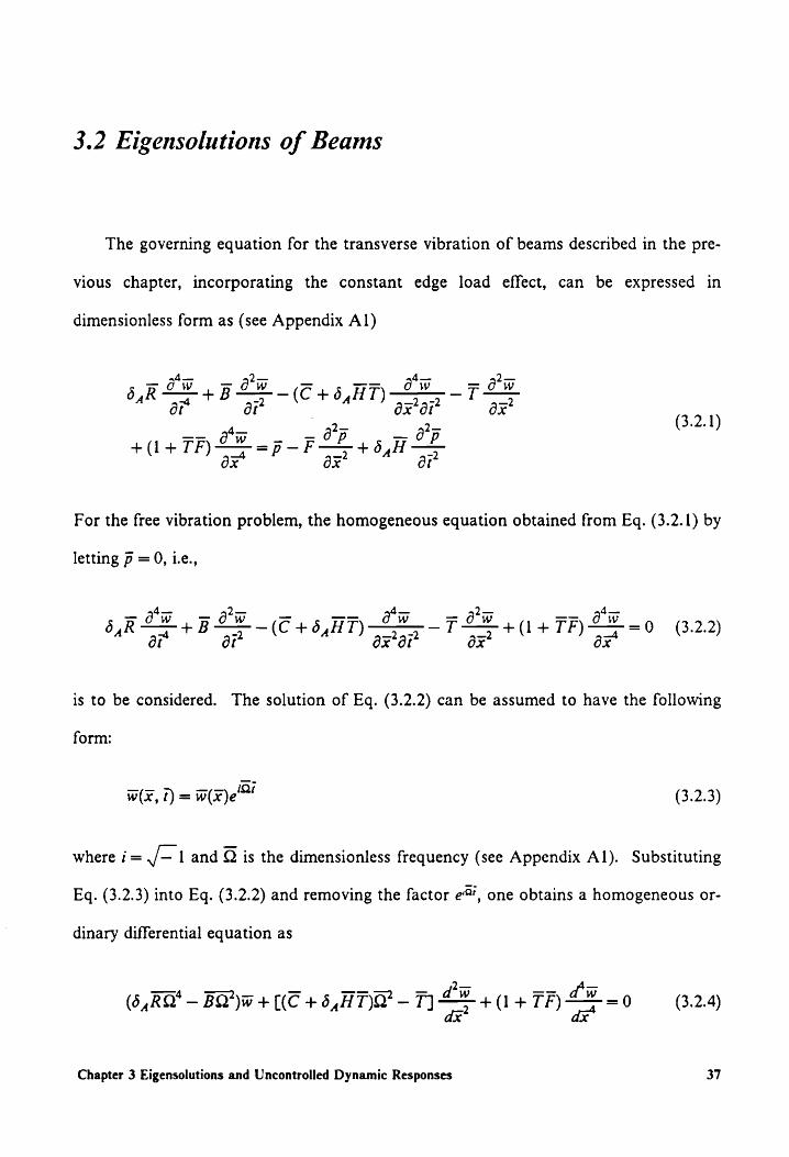
The governing equation for the transverse vibration of beams described in the pre-

vious chapter, incorporating the constant edge load effect, can be expressed in

dimensionless form as (see Appendix A1)

_ ats 2 ate _ ato 54R + B22 HT) =e - +

i f

aw _ ap _ ap (3.2.1)

+(1+TF) wet TP Ft ba Ox Ox Ot

For the free vibration problem, the homogeneous equation obtained from Eq. (3.2.1) by

letting p = 0, Le.,

ow 7 aw oo =aw oe +BY -(C+ 6441) a ~7FTO*8404THH=0 (3.2.2) 6,R “ar ar eer ax’ ax’

is to be considered. The solution of Eq. (3.2.2) can be assumed to have the following

form:

W(X, f) = w(x)e (3.2.3)

where i= J- 1 and Q is the dimensionless frequency (see Appendix Al). Substituting

Eq. (3.2.3) into Eq. (3.2.2) and removing the factor e, one obtains a homogeneous or-

dinary differential equation as

(6, RQ’ ~— BQ) w + [(C +6,HT)Q@ — T] £e 4(1¢+¢TAf2-0 = 63.24) dx"


This ordinary differential equation, together with the associated boundary conditions, is

called the eigenvalue problem [84].

It is known that the solution of Eq. (3.2.4) can be expressed as

w(x) = ae (3.2.5)

where @ is an arbitrary real constant. Substituting Eq. (3.2.5) into Eq. (3.2.4), and re-

moving the factor e”*, one obtains the following characteristic equation:

(1+ 7F\m + ((C +6,H1)Q* — Tm + (6,RQ' — BQ’) =0 (3.2.6)

The roots of this characteristic equation are found to be

—2 _ l _,;) a2 _ =Eys pOt _ RO? m= oe | O, + JO? - 411 + TF\(6,RQ! — BQ?) } (3.2.72)

where

0, =(C + 6,HT)Q -T (3.2.76)

Note: In order to simplify the notation, henceforth the bars which identify the

dimensionless quantities are removed except where it is necessary to make such a dis-

tinction.

Related to the eigensolutions of beams, two cases are considered

Case 1: 6, = 0 (i.e., the rotatory inertia effect is neglected)

In this case, Equations (3.2.7) are reduced to

m= | 1 + Jt +4(1+ TF)BQ") + (3.2.82)


Q,=CX’-T (3.2.8)

Denote

a? = W+TH | ~0,+/[0? +4(1 + TABQ? i (3.2.9a)

f= TT 12, + /[0? + 4(1 + TABQ?) } (3.2.96)

In view of Eqs. (3.2.7a), (3.2.8) and (3.2.9), one can express the roots of the character-

istic equation as

m, m=+.e (3.2.10a)

mM, m= + iB (3.2.10)

where a and # are real and positive. The general solution of Eq. (3.2.4) (with 6, =0),

according to Eqs. (3.2.5) and (3.2.10), is given by

w(x) = a, sinh ax + a, cosh ax + a; sin Bx + a, cos Bx (3.2.11)

Consider the case of simply supported beams. Their boundary conditions can be

shown to be

d° w(x) dx?

w(x) = = 0, atx=0, | (3.2.12)

Impose the above boundary conditions on the general solution given by Eq. (3.2.11).

Then, in order to have a nontrivial solution, one finds that the following frequency

equation


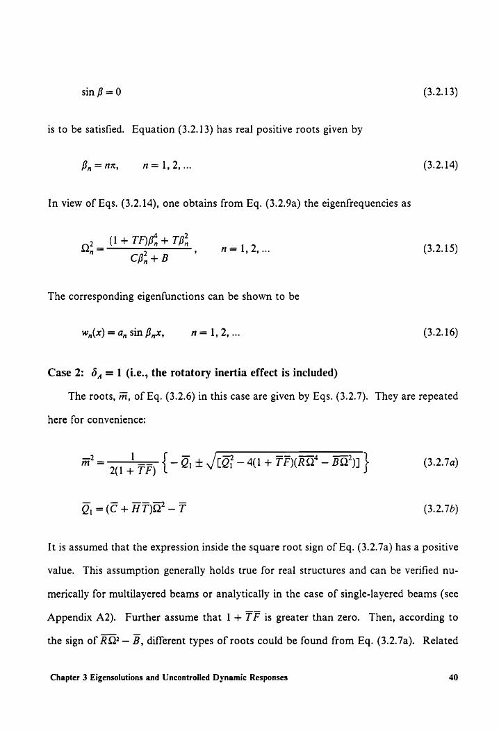
sin 8 =0 (3.2.13)

is to be satisfied. Equation (3.2.13) has real positive roots given by

Bb, =n7, n=1,2,... (3.2.14)

In view of Eqs. (3.2.14), one obtains from Eq. (3.2.9a) the eigenfrequencies as

_ (1+ TAB, + TB, Q?

. Cp.+B n=1,2,... (3.2.15)

The corresponding eigenfunctions can be shown to be

w,(x) =a, sin B,x, n=1,2,... (3.2.16)

Case 2: 6, =1 (i.e., the rotatory inertia effect is included)

The roots, m, of Eq. (3.2.6) in this case are given by Eqs. (3.2.7). They are repeated

here for convenience:

—2 _ l _,) a2 FE Pot _ RO2 m= oe | 0, + JO? - 4(1 + TF RQ! — BQ?) i (3.2.7a)

QO, =(C + HT)Q’ -T (3.2.76)

It is assumed that the expression inside the square root sign of Eq. (3.2.7a) has a positive

value. This assumption generally holds true for real structures and can be verified nu-

merically for multilayered beams or analytically in the case of single-layered beams (see

Appendix A2). Further assume that | + 7F is greater than zero. Then, according to

the sign of RQ? — B, different types of roots could be found from Eq. (3.2.7a). Related


to this, two cases are considered (again, the bar identifying the dimensionless quantities

is removed):

(A) RQ? — B<0, i.e, N2< +

As in Case 1, define

a? = a7 } ~0,+,/[0? —4(1+ TARO! — BO?) \ (3.2.17a)

p= 3+ 75 12 + /[0? —4(1 + TA(RO! — BQ%)] } (3.2.17b)

It should be noted, however, that Q, considered here is given by Eq. (3.2.7b). The roots

of the characteristic equation, in view of Eqs. (3.2.7) and (3.2.17), can be expressed as

mM, m=+a (3.2.18a)

mM, m= + if (3.2.18)

As a result, the general solution of Eq. (3.2.4) can be written as

w(x) = a, sinh wx + a, cosh ax + a; sin Bx + a, .cos Bx (3.2.19)

Note that although Eqs. (3.2.18) and (3.2.19) are the same as those given in Case 1, the

a and £ in these two cases are different.

(B) RQ? — B>0, ie, Q?> z

In this case, further define

ye WTA 12 ~ /[Q? - 41 + TA(RQ* — BO) \ (3.2.20)


where Q, is given by Eq. (3.2.7b). The roots of the characteristic equation, in view of

Eqs. (3.2.7a), (3.2.17b) and (3.2.20), can then be written as

m, m= + iy (3.2.21a)

mM, mM, = + iB (3.2.215)

where y and £ are real and positive. According to Eqs. (3.2.5) and (3.2.21), the general

solution of Eq. (3.2.4) can be expressed as

w(x) = a, sin yx + a, cos yx + a; sin Bx + a, cos Bx (3.2.22)

Consider the case of simply supported beams. It can be shown that for both Case

2A and Case 2B, there are two frequency spectra associated with each mode. They are

given by

Qin n= Ze {OF VG -4RO,)}, — 2=1,2,... (3.2.23a)

where

Q,=(C+ HTB, + B (3.2.236)

0,=(1+ TAS +TS, Brann (3.2.23c)

The eigenfunctions corresponding to these two frequency spectra are given by

w,(x) = a, sin B,x, n=1,2,... (3.2.24)

which are the same as those in Case 1.


Although for simply supported beams the expressions for eigenfrequencies as well

as eigenfunctions remain the same for the entire frequency range, this is not true for

other kinds of boundary conditions (see, for example, [86,87]). In the latter case, the

expression of eigenfunctions in Case 2A is different from that in Case 2B. The frequency

which separates Case 2A and Case 2B is known as the shear cut-off frequency [51]. This

frequency is equal to Q? = B/R for the beam considered here.

3.3 Dynamic Response of Beams

AS in section 3.2, two cases are considered.

Case 1:6,=0

For this case the governing equation of beams, equation (3.2.1), is reduced to

a’p =p-Poy (3.3.1)

aw ow aw ow Boe CTS Lt TT ar’ ax7ar? ax? ( *) ax4

Before applying the modal analysis technique to determine the dynamic response of

beams, first, one must find the orthogonality conditions associated with eigenfunctions

(for a more general discussion of this approach, see Appendix A3 and [84)]).

Orthogonality Conditions of Eigenfunctions

It was shown in section 3.2 that the eigensolutions (w,(x), Q,) must satisfy Eq. (3.2.4)

(with 6, = 0), 1e.,

dw, 4 > — BQrw,, = 0 (3.3.2)

dw, dx’

(1 + TF) + (CQ —T)


Suppose that (w, Q,) and (w, 22.) are two distinct pairs of eigensolutions and denote

a’w, 2

I],= ( — T) 2 _ BQ; w= 0 (3.3.3a)

dx

dw, d*w, 2 n= (1+ TA 1 +.(cQ?- Ty ~ BO} =0 (3.3.36)

In view of Eqs. (3.3.3), one can form an integral as

1

| (T1,w, -_ IT») dx =0 (3.3.4)

0

Performing the integration by parts on Eq. (3.3.4), one obtains the following equation:

2 nrnll dy ay,

0

dx

dw a dw, qd d d’w " w 4 d’w Ww ; (ma a hth Ga ae (3.3.9)

dx dx x dx

dw, dw dw dw 20 aM J { a] + CLQjw,—— — Qrw, dx — Jo + Tw — dx de 19

where [ ]} represents the difference between the values of the expression inside the

bracket evaluated at the boundaries | and 0.

Further assume that the terms associated with boundary conditions are zero, which

is true for beams with simply supported ends. Hence, from Eq. (3.3.5), one has

2 arnft,. dm ay (0? — 02) I (CA — + Bw) de =0 (3.3.6)


Since Q;4Q, was assumed, in view of Eq. (3.3.6), one finds the following orthogonality

condition:

[ct Bww,) dx =0 3.3.7 | dk at ww) dx = (3.3.7)

However, if i= / , equation (3.3.7) is no longer zero and will be denoted as N;:

N= [ye a 4 ato)" dx (3.3.8)

Next, consider the integral

I

| Mywjdx=0, 9 idj (3.3.9) 0

Equation (3.3.9), after integration by parts is carried out, can be expressed as

[ term fet pm of (co 4 Bu) d ttt aa t dx ax ~ 27} dx dx + Bim) ae

(3.3.10) dw, 1 dw, d’w

= (1+ TF) [— wa bo tle Lb — (CQ Nowy hy ae t J dx 70

In the case of simply supported beams, the boundary terms in Eq. (3.3.10) vanish and

one has


2 f' ler d’w, dw, 7 au dw, 1

ta ae dx dx *

(3.3.11) 2 1 dw; dw,

- 93] (C7 at Bum) dx =0 0

In view of Eqs. (3.3.7) and (3.3.11), one obtains another orthogonality condition:

I aw, dw, dw, dw, wh:

j (1 + TF) ie Tet TT ae dx = 0, ix] (3.3.12)

If i=, equation (3.3.12) is no longer zero. Then, from Eqs. (3.3.8) and (3.3.11) one has

2 2 1 1 dw; 2 dw, 2 -

= 5, i J+ 7H ated, i= 1,2... (3.3.13)

where Q, are the eigenfrequencies.

Modal Analysis and Dynamic Response

The modal analysis is a technique that makes use of the orthogonal property of

eigenfunctions to convert the governing equations of structures (which generally are

partial differential equations) into an infinite denumerable sets of uncoupled modal

equations. Because modal equations are a set of independent ordinary differential

equations, they are much easier to be used to study the response of structures. More-

over, since modal equations are related to the modes of vibration, the solution obtained

from these equations could provide a better insight of the structural vibration. In the

following, the procedure of deriving modal equations from the governing equation is il-

lustrated.


First, multiply Eq. (3.3.1) by an eigenfunction w, and integrate it through the whole

length of the beam. This yields

1 2 4 2 4 O'w Cw O*w Ow

Bm -—- C—_ — — TH (14+ T. w. ax ik ar ax’ar? ax’ iz ax* ’

(3.3.14) 1 a?

-| (p — F—4 )w, dx 0 Ox

According to the expansion theorem [84,85], w(x, rf) can be expressed in an infinite series

form as

w(x, ) = Daal )ea(*) (3.3.15) n=}

where w,(x) represent eigenfunctions and q,(t) are generalized coordinates (which are also

called natural coordinates [84,85]). Substituting Eq. (3.3.15) into Eq. (3.3.14), per-

forming the integration by parts and taking into account orthogonality conditions de-

rived earlier, one obtains the following modal equations that correspond to Eq. (3.3.1):

G+ Qh4=fe, r= 1,2,... (3.3.16a)

where

1 3?

fo=t | Ww, p-F— dx (3.3.165) N, Jo Ox

in which WN, are the norms defined by Eq. (3.3.8).

For convenience, the eigenfunctions are normalized as follows:


1

[ woo ae = l, r=1,2,... (3.3.17) 0

Denote ¢,(x) to be the normalized eigenfunctions which in the case of simply supported

beams can be shown to be

o,(x)=/2 sinBx, r=1,2,... (3.3.18)

In terms of the normalized eigenfunctions, the modal forces f,, can be expressed as

2 1 f? O"p fr =F | Op — FZ) dx (3.3.19a) ro Ox

where

N,= CB +B (3.3.195)

When the beam is assumed to exhibit the proportional viscous type damping, the

modal equations described by Eq. (3.3.16a) must be modified as (see Appendix A3)

Gr + 26,2,4,+ 2,°4,=far r=1,2,... (3.3.20)

where €, are the damping ratios. The solution of Eq. (3.3.20) can be shown to be [84]

e7 FH sin Qa,t G,(0) 1 ft. geen |: 1 at) = — | filo Fl) sin Q(t — t) dt t a,

g (3.3.21) +e ae) cos Q.,t + —==— sin a4} q,{0), r=1,2.,...

J1-@


where Q,, = Q,./1 — €2 denote the damped frequencies.

Next, the dynamic response of the simply supported beam that is initially at rest and

subjected to a traveling load is considered. The traveling load is defined as follows:

Pod(x — vt) coswmt, O< wl P(x, 1) = (3.3.22)

0, vti> 1

where 6( ) denotes the Dirac generalized function, p, is the amplitude, v is the traveling

velocity, and w is the forcing frequency. The modal forces, according to Eqs. (3.3.19)

and (3.3.22), are given by

(1+ BF) sin Bvt cos wt, O<ts 4 (3.3.23a)

J 2 po

N r Salt) =

and

Salt) = 0, i> (3.3.235)

In view of Eqs. (3.3.21) and (3.3.23), the generalized coordinates are found to be (note

that 4,(0) = 4,(0) =90 )

2 f

q(t) = Lm (1+ BF | eW FAM) sin Ot — 7) sin Bvt cos wr dr (3.3.24) r 0

for the time period O<¢<1/v. When ¢>1/v the beam is no longer subjected to the

traveling load. Hence, the beam is in free vibration whose amplitude will decay gradually

due to the presence of the small damping in the structure. The response for ¢> 1/v can

be determined from Eq. (3.3.24) by replacing the upper integration limit by I/v.

Case 2: 6, = 1


The governing equation of beams in this case is given by Eq. (3.2.1). For conven-

ience, it is repeated here:

ow w aw aw aw aw —7 + B= - (C+ AT) a7 iT 7 + (1+ TF) a

art ar? ax’ at Ox Ox 3 7 (3.2.1)

ax? ar?

First the conditions of orthogonality associated with eigenfunctions are derived.


As in Case 1, consider two different pairs of eigensolutions (w,, Q,) and (w,, Q,)

where Q, could represent either the first or the second branch of the frequency spectra.

In view of Eq. (3.2.4), the following relations hold true:

d°w, 4 2 I, =( ~T] — t (RQ* — BQ?)\w,=0 — (3.3.25a) x

d’w, 4 2 =(1 —T] wee + (RQ? — BQ2)w,=0 (3.3.256)

In view of Eqs. (3.3.25), an integral can be formed as

1 i} {TI,w, — I1,w,} ax =0 (3.3.26)

0

After performing the integration by parts and imposing the simply supported boundary

conditions on Eq. (3.3.26), one obtains

= dw,

dx (a? -92)| | Bn +(C+H th ax — (95 —Q )| Reem, dx=Q (3.3.27)

0


Since 2,40, the factor Q2? — Q? can be removed from Eq. (3.3.27) and one obtains

w, dw, 1 dw, 1 | | Burs + (C+ Hl) — \ ae (QF + Q?) | Rw,w,dx=0, Q,4Q, (3.3.28)

0 0

Now suppose that j=r=s (i.e, only the jth mode is considered) and let

Q,= Q,, and Q,=Q,, shown in Eq. (3.3.28). In this case, the integrals in Eq. (3.3.28)

yield positive real values and will be denoted as

1

Ny= | R(w))’ dx (3.3.29a) 0

N [43 recA ty a 3.3.29b y= J (mw) + (C+ HT) J" ¢ dx (3.3.295)

Then, according to Eqs. (3.3.28) and (3.3.29), the following relation is obtained:

N. 2 2 y Oy + Oy =a (3.3.30)

One should be reminded that Q,, is in the first spectrum (the one having the smaller

value) and Q,, in the second spectrum associated with the jth mode of vibration.

When the normalized eigenfunctions $(x) are used, equations (3.3.29) can be ex-

pressed as

Ny=R (3.3.31)

Noy =(C+ HT)B; + B (3.3.31)

Chapter 3 Eigensolutions and Uncontrolled Dynamic Responses $1

In view of Eqs. (3.3.30) and (3.3.31), one has

(C+ HTB; +B OQ, + Q3) = (3.3.32)

The validity of the above relation can be verified by using the eigenfrequencies given by

Eqs. (3.2.23).

However, if the modes are different (1.e., rs), according to Eq. (3.3.28) the follow-

ing orthogonality conditions

[42 c+ HT) ee el = 0 3.3.33 0 ww, + ( + T) dx dx x= (3.3. a)

1 | Rw,w, dx = 0 (3.3.335)

0

must be satisfied.

Next, consider an integral of the form

1

| II,w, dx =0 (3.3.34) 0

After performing the integration by parts and imposing the simply supported boundary

conditions on Eq. (3.3.34), one finds

1 | dw, dw 4 2 r 5 ar] Rw,w, dx — a] Kc + HT) Tk ax t Bw.) dx

{ patna be, pate ds |, =0 (3.3.35) + ; (1 + TF) me at +T— Ix


Taking into account the orthogonality conditions given by Eqs. (3.3.33), one obtains

from Eq. (3.3.35) another orthogonality condition:

1 dw, d’w, dw, dw, [usm me det +T ax dx dx =0

If r= s, equation (3.3.36) is no longer zero and will be denoted as

m= [a+ ry Sep ey = — —_— Ix * 0 dx* ax

Then, according to Eqs. (3.3.29), (3.3.35) and (3.3.37), one has

N,Q; — No,Q; + Ny, =0

The roots of Eq. (3.3.38) are given by

l / Qi, Q3, = 2M, {Nu + (N>,)° _ 4N,,N3, i

When normalized eigenfunctions $,(x) are used, equation (3.3.37) becomes

N3,=(1+ TAB, + TB;

(3.3.36)

(3.3.37)

(3.3.38)

(3.3.39)

(3.3.40)

It can be shown that when N,,, N,, and N,, in Eq. (3.3.39) are replaced by those given

by Eqs. (3.3.31) and (3.3.40), one obtains exactly the same eigenfrequencies described

by Eqs. (3.2.23).



Following the exact procedure described in Case 1, and imposing the simply sup-

ported boundary conditions as well as the orthogonality conditions of eigenfunctions,

one obtains the modal equations corresponding to Eq. (3.2.1) as

Gr + 119 + Ndr = Sar r=1,2,... (3.3.41a)

where

if ap ap =— — F—+ H— ) ax 3.3.415 Sar N,, 0 $,(p ox? ar ) ( )

N2, N3, = ; = 3.3.41c Nir Ni, N2r Ni, ( )

The impulse response function associated with the system described by Eqs. (3.3.41) can

be shown to be

sin Q),4-— I l 1.

(1) = sin Q 3.3.42 ” 03, — 23, Qs, Q), a ( )

Again, assume that the beam initially at rest is subjected to a traveling load defined

by Eq. (3.3.22). The modal forces can be found by substituting Eq. (3.3.22) into Eq.

(3.3.41b), which yields

J2 po Sit) = R {Tl + Fg? - H(" + Bev’) cos wr sin Bvt

—2Hwf,v sin wt cos Bvt}, O<est

(3.3.43a)

and


(3.3.43)

According to the convolution integral theorem, the generalized coordinates q(t) could

be determined from the following integral equation:

iA) = | O10 nr (3.3.44)

In what follows, the eigensolutions and uncontrolled dynamic response of plates are

studied.

3.4 Eigensolutions of Plates

The governing equation for the transverse vibration of plates can be expressed in

dimensionless form as (see Appendix A4)

5.2 ow 5 Ow on aw A <4 +B— a (C1 + 54HT)) a y (G+ 6,HT)— G5 Par

ot 7? x*ar at

-~(T,4 + ws Ty ow 7 )+ (D, + T)F)) “ +(2+T\F, + vod (3.4.1) ax ay’ ax’ ax ay

+ (D, + TF) ae PA ths —)45,H dy Ox oy

To find the eigensolutions, consider the free vibration problem described by

35 Chapter 3 Eigensolutions and Uncontrolled Dynamic Responses

5,R ae 5 2B W (C46 AT) 2 (C, +5,HT,) A A 1 ax" a7 2 A 2 ayer

2— 2— 4— 4—

-(F, 22 47,2%)+0,4 ees OW 247A + TFA 3.42) Ox Oy

ax’

Te + (Dy + TF) =0

The solution of Eq. (3.4.2) can be assumed to have the following form

(3.4.3) W(F, 7, 1) = w(x, pe

Substituting Eq. (3.4.3) into Eq. (3.4.2) and removing the factor e’, one obtains

(5, RQ ~ BQ*)w + (Q°(C, + 6,HT,) — Ty} xa x

aya OT Ow LE ew + {Q'(C, + 64HT)) — T3} a + ( —= (3.4.4)

ow 4—

+ (24+ TF, + LA) a+ (D, + T,F,) F =0 iy ay

Due to the presence of the term 0*w/dx?dy*, equation (3.4.4) cannot be solved by

using the method of the separation of variables. Introduce the nondimensional 2D

Laplace operator

a? 1 2 3 =fA= + 3.4.5 1 x? ( ep ) ay? ( )

Then, in the case that 7, = T; (hence, 7, = 7,72, ¢, = ¢,/¢,), equation (3.4.4) can be ex-

pressed as

(3.4.6a) 0, AAW + O,,Aw + O,,0 =0

56 Chapter 3 Eigensolutions and Uncontrolled Dynamic Responses

where

0,,=D,+ TF, (3.4.6)

Qn = (C, + 5 4HT,)Q -T, (3.4.6c)

On3 = 5 4RQ’ — BQ’ (3.4.64)

Equation (3.4.6a) can be written in a product form as

(A + G,,)(A + G,)w = 0 (3.4.7a)

where

{On + \/ Dp — 49y12p3 i (3.4.76) Gy, G Gy = a

P

Note: As before, for simplicity, the bars indicating the dimensionless quantities are re-

moved.

For eigensolutions of plates, two cases are considered.

Case 1:6, =0

Accordingly, equations (3.4.6b), (3.4.6c) and (3.4.6c) are reduced to

Q»1 = D, + TF, (3.4.82)

On = C,Q’ -T, (3.4.85)

Q,3 = — BQ? (3.4.8c)

respectively. Denote


Sf = FG {Opa + V Opa — On Opa } (3.4.94)

$= FH {On -V/ Oa — 4092 } (3.4.98)

The value of the expression inside the square root sign generally is positive (note when

T, 1S negative, 1.e., a compressive force, its magnitude is assumed to be far smaller than

that of the buckling load). In view of Eqs. (3.4.9), one could also express Eq. (3.4.7a)

as

(A + s?)(A — s?)w(x, y) = 0 (3.4.10)

Equation (3.4.10) can be written in the form of two separate equations as [84]

(A —s})w = w, (3.4.11a)

(A + s;)w, =0 (3.4.11)

Hence, the solution of Eq. (3.4.10) can be expressed as

w= Wht Wy (3.4.12)

where w, is the solution of the homogeneous equation

(A — s3)w, = [A + (is,)*]w, = 0 (3.4.13)

Equation (3.4.11b) has the same form as that obtained from the study of the transverse

vibration of thin uniform membranes [84]. It is also clear that the solution of Eq.

(3.4.13) could be found from that of Eq. (3.4.11b) by replacing s, by is, Here, i denotes

the imaginary unit ./—1.


It can be shown that the general solution of Eq. (3.4.10) is given by

w(x, y) =c, sin a,x sin ?pBy + c, sin a,x sin OpB yy

+c; cos a,x sin?’ pBhyy + cy cos a,x cos Opfiy

+ cs sinh a,x sinh ?pfay + ce sinh a,x cosh @pfy (3.4. 14a)

+ c7 cosh ax sinh /phoy + cg cosh a,x cosh ?pfoy

where

a+ Bias + B= 3 (3.4.14)

and a,, &, B,, B, are real and positive.

Consider the case of simply supported plates. The boundary conditions can be

shown to be

a*w w=—, =0 along x = 0, | (3.4.15a)

Ox

a7w w=" 9 along y=0, 1 (3.4.155)

y

Imposing the above boundary conditions on the general solution, in order to have a

nontrivial solution, one finds that the following frequency equations

sin a, = 0 | (3.4.162)

sin? pf, =0 (3.4. 165)

must be satisfied. These frequency equations have positive real solutions given by

Lim = mn, m=1,2,... (3.4.17a)


Bn=—z n=1,2,... (3.4.17)

According to Eqs. (3.4.9a), (3.4.14b) and (3.4.17), the eigenfrequencies associated with

mode (m, 2) can be shown to be

2 Diein+ Bin. Filein + Bin) + (tim + Bin) G.4.18) n — 1 e °

™ B+ C\(@im + Bin) B+ C\(im + Bin)

The eigenfunctions are obtained as

Wan(X, ¥) = Cnn SIN Max SiN ny, m,n=1,2,... (3.4.19)

Case 2:6,=1

In this case, one must consider Eqs. (3.4.6) and (3.4.7). The expression inside the

square root sign in Eqs. (3.4.7b), 1.e.,

Ona = Orn ~~ 4051 Qp3 (3.4.20)

= [(C, + 6,HT,)Q — T,} — 4(D, + T,F,)(6,RQ* — BQ),

generally can be assumed to be positive (when there are no edge loads, it can be shown

that C?—4D,R>0 is a sufficient condition for Q,, to be positive). Under this assump-

tion, it can be seen from Eqs. (3.4.7b) and (3.4.20) that G,, is always positive, while G,,

could be positive or negative depending on the sign of RQ?— B. These two cases are

discussed in the following:

(A) RQ?— B<0,ie., Q< =

Denote


3 = a {O50 + x Oa — 40pQpa } (3.4.21)

f= FH {Opa — \ Oa ~ 40n10rs } (3.4.216)

Hence, equation (3.4.6a) can be written in the same product form as Eq. (3.4.10). Asa

result, the general solution derived in Case 1 remains valid here. It should be empha-

sized, however, that although the same notations s, and s, are used in both cases, they

actually represent different quantities (in Case | , 6, = 0).

Consider the case of simply supported plates. Again, equations (3.4.16) and (3.4.17)

in Case | still apply to this case. According to Eqs. (3.4.14b), one has

aim + Bin = Simn (3.4.22)

Then, by making use of Eqs. (3.4.6b-d), (3.4.17), (3.4.21a) and (3.4.22), the

eigenfrequencies are obtained as

Qn» Vin = Soe (Ops F x) 3s — ARQ ps } (3.4.234)

where

Ons = B+ (Him + Bin(C, + HT;) (3.4.23)

One = (im + Bin(D + Ti, + Ti) (3.4.23¢)

The eigenfunctions are the same as those given by Eq. (3.4.19).

(B) RQ? — B>0, ie, Q? > +

In this case, further define


$= FO {Opa — \ Opa — 4010p | (3.4.24)

Equation (3.4.7a), in view of Eqs. (3.4.21a) and (3.4.24), can be written as

(A + s*)(A + s2)w(x, y) = 0 (3.4.25)

Following the procedure described in Case 1, one obtains the general solution of Eq.

(3.4.25), which can be expressed as

w(x, y) = c, sin a,x sin ?pfiy + c, sin a,x sin /pByy

+c; cos a,x sin? pBhy + cq cos a,x cos Opfyy

+ cs Sin a3x Sin OpBay + Cy SIN 43x COS OpBry (3.4.26a)

+ cz COS 03x Sin Hp ay + Cg COS 03x COS PpBay

where

af+ Bi =s7; 03+ Bp =53 (3.4.266)

Consider the case of simply supported plates. It can be shown that in this case the

following frequency equations are found:

sin a, sina; =0 (3.4.27)

sin ¢ pf, sin? pf; =90 (3.4.27)

Since s? ¥ s?, it can be seen from Eqs. (3.4.26b) that generally a? # a2 and f?# £3. Asa

result, according to Eqs. (3.4.27), the eigenfrequencies should be determined either from

sina, =0 (3.4.28a)

sin ?p6, =0 (3.4.285)


or from

sin a, =0 (3.4.29a)

sin ?pf, =0 (3.4.295)

Since Eqs. (3.4.28) are the same as those obtained in Case 2A, the eigenfrequencies given

by Eqs. (3.4.23) remain valid in the present case. Although not shown here, the same

results are obtained when Eqs. (3.4.29) are used. The eigenfunction expression obtained

in this case again is the same as that given by Eq. (3.4.19).

3.5 Another Method of Finding Eigenfrequencies

The analytical method of finding eigensolutions considered in the previous section

can be applied to the plate with various boundary conditions. However, it was shown

there that this approach will work only for the case in which the edge loads acting in two

in-plane directions are equal and have the the same sign. As for the cases with uniaxial

or unequal biaxial loads, the problem can not be solved by such a method. Since only

simply supported plates are treated here, the Navier’s method can be used to determine

the eigenfrequencies. In the latter approach, the restrictions on edge loads can be re-

moved. To apply Navier’s method, first, one chooses admissible functions of the fol-

lowing form (they were shown to be the eigenfunctions of the cases considered in section

3.4):

Waan(X) VY) = Cnn SiN Mrx Sin ny, m,n=1,2,... (3.5.1)


The admissible functions given by Eq. (3.5.1) satisfy the simply supported boundary

conditions.

Next, one expands w(x, y) in terms of these admissible functions as follows:

w(x,)) = >.) Cn, Sin max sin nny (3.5.2) m=) n=1

Substituting Eq. (3.5.2) into Eq. (3.2.4) and applying the Galerkin procedure [96], one

obtains

(6 4RQnn — BQan) — (mn) {(C, + 54HT,)Q7,, — Ty} — (nn)"{(Cy + 6 4HT,)Qran — Ty} + (mn)*(D, + TF;) (3.5.3) +n n'(2 + TF, + T2F;) + (na) (D, + TyFy) = 0

To obtain Eq. (3.5.3), the following orthogonality condition was used:

irl CmnCr | | Wmn(X Y)Wrs(X, y) dxdy = = OmrOns (3.5.4) 0~0

where 6,, denotes the Kronecker symbol which takes the value of | if r=s and zero

otherwise.

Based on Eq. (3.5.3), two cases are considered.

Case 1:6, =0

Accordingly, equation (3.5.3) 1s reduced to

{B+ C\(mn)* + C,(mn)3Q2,, = T,(mn)? + Ta(nny* + (D, + T,F,)(nny 3.5.5

+ (2+ 7, Fy + T,F,)(mn) (nz) + (Dy + T,F,)(nx)* (3.5.5)

From Eq. (3.5.5) one obtains the eigenfrequencies as


= 7 (T (a2, + or Bn) + (Dy + T.Fi)n [B+ C,(a?,+—)] R

or (3.5.6a)

] Tp 2 72 l Trp + [2+ 7, F,( —+— )]a2 Be + (— 4+ TF, — 2+ TA +a Memba + (py, ia Pr

where

t, 2 T, op = ey ’ Tp =¢2——- T, > Xp, = MT, B,=ann (3.5.65)

It can be shown that when 7,=1 one obtains the same result as that given by Eq.

(3.4.18).

Case 2: 6,=1

In this case, from Eq. (3.5.3) one finds

l Qanr Ginn = Fie 4 Ops F v/ Ops — ARQ ps } (3.5.72)

Here

Ops = B+ am(C, + HT) + BA(C, + HT) (3.5.76)

On = om 7} + BrTy + an( Dy + T,F;) 2 (3.5.7c)

+ a7,By(2 + TF + TF) + By(D, + TF)

If one lets 7, = 7,72 in Eqs. (3.5.7), one obtains the same results as given by Eqs.

(3.4.23).


3.6 Dynamic Response of Plates

Again, two cases are considered here.

Case 1:6,=0

Accordingly, the governing equation described by Eq. (3.4.1) is reduced to

a*w aw a*w aw a*w Be - ce ro IT +7,—% ar! axa? aytar? ia tf ay

+(D, + TF) 2% + (2+ 7, F,+ T,F,) + (Dy + T,F,) aw (3.6.1) Ox Ox’ dy oy

a’p a*p =p-(F, —— +i — P ( 1 ax? 2 ay )

As in the case of beams, first, the orthogonality conditions of eigenfunctions are derived


The eigensolution (w,,(X, y), S2nn) Satisfies Eq. (3.4.4) (with 6, =0 ), Le.,

4 4 4

O Wan O Wan O Win Tan = (D, + TF) 4 +(2+ 7, Fy + TF) 7. 2 + (D, + T,F,) —7—

Ox Ox dy 0 tw zw (3.6.2a)

+ (CQ, — T)) = + (C2Qiin — T) F 7 — BQrnWnn = 9

Let (w,,(x, y), Q,,) be another pair of eigensolutions such that 2,,4#Q,. Hence, one has

4 4 4

aw, aw, aw, IT,, = (Dy + Fy) a t+ (2 + TP + Thy) ary t+ (P21 + Thy)

Ox Ox’ dy oy > 2 (3.6.25)

2 0 Wrs 2 0 Wrs 2 + (C,2;, — T)) + (C,2;, — T) 7 BQ;,W,s = 0

ax? oy


Now form an integral as follows:

1fl

[ [thas Tenn Ady (3.6.3) 0~0

From Eq. (3.6.3), after performing the integration by parts and imposing the simply

supported boundary conditions, one obtains

3 Ow,, Onn OW OW m2) | C= ax Ox + C, ay ay —— + Bw,,Wnn? axdy=0 (3.6.4)

Since Q,, # Q,, was assumed, in view of Eq. (3.6.4) the following orthogonality condition

is obtained:

[I] c, itm Ors | Own Ors p dxdy =0 3.6.5 odo 1 Ox ox * 1 dy ay + WmnWrs xay = (3.6.5)

When m=n and r=s (hence Q,,=Q,,), the integral given by Eq. (3.6.5) is no longer

zero and will be denoted as

Nimn = | | | tau OWmn 4 cy Senn? + Ban} dxdy (3.6.6) 040 Ox oy

Next, examine the integral of the form

ipl | | Tans axdy = 0 (3.6.7) 00


From Eq. (3.6.7), after performing the integration by parts and imposing the simply

supported boundary conditions, one obtains

[ [iw + TF) oe on Sn 24 TF + TF.) Ws Onn odo ax? ax? pp SE" axdy axdy

os 8° Wan AW, OWmn OWrs Pn, + (D, + T,F,) — —— } dxdy (3.6.8)

ay |x ax °? ay

; , Ow dw,, a Saal [GEG GET + tan ad = 0

In view of Eqs. (3.6.5) and (3.6.8), another orthogonality condition

if oe Oran 6°w,. a? Wann J J {(D, + T,F,) — Ae — + (2+ T,F, + T,F,) = axdy “Gxay

3.6.9 Dee on, “au Wn rs 8Wmn Ore BW yy G9)

+ ( 2+ yf) —— ay? ay? ~ 4] ax Ox ~~ 42 éy éy } vay

is obtained. When m=randa=s, the integral given by Eq. (3.6.9) is no longer zero

and will be denoted as

2 2

N. =| [wo + TF OT Wrnn Y4 (24+ TF + Fy OW mn y 2mn 040 1 71 ax? 2 2° 1 axdy

, (3.6.10) (Dy + T)E ee = 7 ee ry Se YY de 2 2° 2 ay? 1 Ox 2 éy iy

Then, in view of Eqs. (3.6.6) and (3.6.10), one obtains from Eq. (3.6.8) the following re-

lation:

(3.6.11)



To find the modal equations corresponding to Eq. (3.6.1), first, let’s expand the

transverse displacement in the following form:

W951) = YY dal) Wan) (3.6.12) m=! n=]

where w,,,(x,y) denote the eigenfunctions and q,,(t) are the generalized coordinates.

Next, one substitutes Eq. (3.6.12) into Eq. (3.6.1) and applies the Galerkin procedure.

Then, performing the integration by parts, and imposing the orthogonality conditions

as well as the simply supported boundary conditions on this last equation, one obtains

Gan(t) + andmn(l) =Simn(0)s m,n=1,2,... (3.6.13a)

where

1 fir ap ap Lana) =A || ante — (Fi 2 + 2) dedy (3.6.136) Imn ¥9 40 Ox oy

It has already shown in section 3.4 that for simply supported plates the

eigenfunctions are described by

Wan(X, ¥) = Cnn, SIN Mrx sin ny

For convenience, the eigenfunctions are normalized such that

lft

I | we (x,y) dxdy = 1 (3.6.14) 0


Denoting the normalized eigenfunctions as @,,,(x, y), one has

Pm,(X, ¥) = 2 Sin mnx sin nny (3.6.15)

In terms of @,,,(x, y), the N,,,, can be shown to be

Nimn = Ci(mny + C,(nn)* + B (3.6.16)

When the plate is assumed to exhibit the proportional viscous type damping, the

modal equations described by (3.6.13a) must be modified as

Gal!) + 2 mnQmndmnlt) + Qn Inn) =Samn(), mi, n= 1,2,.. (3.6.17)

where €,,, are the damping ratios and /,,,(f) the modal forces given by Eq. (3.6.13b). The

solutions of Eqs. (3.6.17) when normalized eigenfunctions are used can be shown to be

l ‘ - —t). inall) = Ga | Lana(t}e~ A si Dapy(t~ 2) n

_ om +e iat} COS Qamnat + = sin nf Qmr(0) (3.6.18)

V Cmn

l

Qlamn

+ ebm! sin OQ annl Gm), r=,

where Q2,,,, = Q,,./1 — €2, denote the damped frequencies.

Assume that the plate initially at rest is subjected to a travelling load defined as

Po cos wt d(x —vt)dy—yo), OS tl

P(x, ) = (3.6.19) 0, ve> 1

The modal forces corresponding to p(x, y, f) can be found by using Eq. (3.6.13b). When

normalized eigenfunctions @,,,(x, y) are used, they could be expressed as


2Po COS wt 4 » . Samn*y) = —N {1 + F,(mz)° + F,(nz)"} sin mavt sin n7yp (3.6.20)

Imn

The generalized coordinates in this case are given by

2Po Imalt) ~~ N, mn {1+ F; (mn) + F,(nz)’} sin mave sin ntyo

Quinn (3.6.21) t

7 bmn mn | ermm® sin QQ mn(t — T) COS wt Sin mavt dt 0

Case 2: 6,=1

Consider two different sets of eigensolutions, (w,,(x, y), 2,,) and (w,,(x, y), Q,,).

Following the procedure that was used in the analysis of beams, for simply supported

plates one obtains the following orthogonality conditions of eigenfunctions:

ipl | | RWynW,s axdy = 0, (3.6.22a) 00

| | | (C+ HT) ome es 4 (Cy + HT) Ce o4y Ox Ox ae * ay ay (3.6.22b)

+ BwynW,s} dxdy = 0

and

2 2 2

[ [ @ +7, F) me Og 024 Ty + TF) odo 1 141 ax? ax? 142 24 1 axdy

o°w,, O° Wan 6°w,. OWan OWrs

axdy + (P2 + Taf) ay? ay’ +I ay Ox

OWmn OWrs ay dy } dxdy =0

(3.6.22c)

+ T,


Furthermore, the norms obtained are defined as follows:

ir |

Nimn = | | Rw? dxdy (3.6.23a) 0°0

ifi Cw Ow

Nomn = | | {(C, + HT,)( ay + (C, + HT.) za + Bw2,} dxdy (3.6.236) 00 y

and

8’ Wann y

Oxd

rel Ow, Nana | | (Ds + TEM St + 2+ THA + TA 9 (3.6.23c)

O° Worn

ay?

Ow Ow 2 2 2 + (D, + TF) y+ T(AY + , } dxdy

As in the case of beams, although there are two frequency spectra associated with

each mode, for simply supported plates one can express the transverse displacement in

a double series form as

w(x, y, t) = » > dnl ®nnl 9) (3.6.24)

m= n=!

To find the modal equations, first, one substitutes Eq. (3.6.24) into Eq. (3.4.1), applies

the Galerkin procedure and performs the integration by parts. Then, imposing on this

last equation the simply supported boundary conditions and taking into account the re-

lations described by Eqs. (3.6.22) and (3.6.23), one obtains

dmn() + Nimn4maD + NamnImnl!) = Samnl?) (3.6.25a)


where

(3.6.25)

1 {' { P_(F a°p r a°p ap ihn= w — — + F, —)+ H— > dxd 3.6.25c Sam) Nimn o%o mn ( 1 ax? 2 ay? ) or iy ( )

When normalized eigenfunctions are used, it can be shown that

Nimn = R (3.6.26a)

Nomn =(C, + HT;)(mn)* + (Cy + HT>)(nz)’ + B (3.6.26)

Nomn = (mn)T, + (nx)?T> + (ma)(nn)’(2 + TF, + T2F;) . : (3.6.26c) + (mn) (D, + T,F,) + (nz) (Dz + TF)

Assume that the plate initially at rest is subjected to a traveling load described by

Eq. (3.6.19). The modal forces obtained from Eq. (3.6.25c), when normalized

eigenfunctions @,,,(x, y) are used, are given by

2Po . 2 2 2 2 Lamn(%s ) = —Q— Sin nayo{[1 + (mn) F, + (n2)'F, — H(w" + mav’)] (3.6.27) cos wi sin mavt — 2Hwmny sin wt cos mrvt}

The generalized coordinates in this case can be obtained from the following integral

equation:

Imalt) = { (3.6.28) 0 nn ~ Qinn

| Samr{t) sin Qi malt _ t) sin Qo mnlt — T) d _ Tt

Qi mn Quinn


Chapter 4 Control System Design

4.1 Introduction

The modal control approach is employed to suppress the vibration of structural

member excited by a certain transient load. The modal control here means that the vi-

bration control is effected by controlling the modes of vibration. However, it is known

(and shown in the previous chapter) that the structural member possesses an infinite

number of modes of vibration. To effectively control all these modes, one might need

to use the distributed control actuator that can exert control inputs over the entire

structure. One type of actuators that might possess such a property is the piezoelectric

actuator [88]. The applications of this type of actuator has attracted a lot of investi-

gation recently. In the mean while the technique of using piezoelectric actuator is still

under development, and such an approach certainly could not universally be applied in

every structural problem that would require the use of control. In this study only

discrete-type actuators are considered.

Chapter 4 Control System Design 74

It is known that the structural vibration is dominated by the lower modes of vi-

bration which are characterized by low frequencies. Hence, generally one can suppress

the vibration very effectively by controlling only these dominant modes. It should be

noted, however, that by designing the control system based on an approximate model

where the effect of the higher modes of vibration is neglected leads to the undesirable

spillover effect [4]. It was shown by Balas [4] that the spillover effect may cause insta-

bility. The spillover effect, however, will not be considered in the present study. The

problem to be investigated here concerns mainly the effect of the modelling error on the

response of the structure which is actively controlled.

The modelling errors being considered are those due to the difference between the

nominal and actual plants, as well as that due to the variation of certain structural pa-

rameters. The nominal plant is the system model which is used to design the controller,

while the actual plant is the system that one actually controls. [In this thesis, the nomi-

nal plant is assumed to be the structural model based on the classical theory (CT) such

as Bernoulli-Euler (beams) and Kirchhoff (plates) theories, while the actual plant is as-

sumed to be that based on the higher-order theory (HOT). The aim hence is to evaluate

the validity of the use of the classical structural model for control system design as well

as to clarify the effect on controlled response of certain important structural parameters.

In this study the control law is designed by using the optimal control theory. In the

following section some theoretical background of optimal control theory applied to the

vibration contro] problem is reviewed. For more detail, see for example [89].


4.2 Linear Optimal Regulator

Assumed that the plant to be controlled only consists of the dominant modes of

vibration of the structural member. This system model incorporating the control inputs

can be expressed in state-variable form as follows:

u(t) = A u(t) + B z(t) + £9) (4.2.1)

where

u(t) the N x I state vector,

A the NV x N system matrix (constant),

B the N x M input matrix (constant),

z(t) the M x 1 control input vector,

£40) the N x | disturbance vector corresponding to the external load.

It is assumed that all the states are available for feedback. Since the objective of

control is to suppress the vibration of the structure, the problem can be formulated as

a linear regulator. The task, hence, is to design a controller which can regulate the states

of the system to be close to the trivial state (i.e., no vibrational motion) in a desired

manner. |

The performance index, which is to be minimized, associated with the linear regu-

lator problem is often chosen to have the following quadratic form:

J= > u(t) S u(t) + = [oo Q u(t) +.27(1) Rz0)dt (4.2.2)


where

yt the initial and final time (both are assumed fixed) of the intended con-

trolling period,

S the weighting matrix for the terminal states u(s,), and is constant, sym-

metric and non-negative definite,

Q the weighting matrix for states, and is constant, symmetric and non-

negative definite,

R the weighting matrix for control inputs, and is constant, symmetric and

positive definite.

It is also assumed that u(¢,) is free, and the states and control inputs are not bounded,

which must satisfy the system equation described by Eq. (4.2.1). The optimal control

law that minimizes the performance index J described by Eq. (4.2.2) with the dynamic

constraint given by Eq. (4.2.1) can be obtained as follows:

Depending on whether or not the external load is known a priori, two cases can be

considered.

Case I: External load f(t) is known

In this case, one can define an augmented performance index including the con-

straint equation given by Eq. (4.2.1) as

J, = > u’(t)Su(t) + J’ 1 + (u’Qu + z’Qz) + 1(Au+ Bz+f,— wy} dt (4.2.3)

where I,(r) is an N x 1 vector consisting of time-dependent Lagrange multipliers (referred

to as the costate vector ([89]).


Denote

, . 1 7 T. T. . g(u, u, Z, 15) = 7 (u Qu+z Rz) + 1,(Au + Bz + f, —u) (4.2.4)

Then the augmented performance index can be written as

t

J,(u, 0, 2,132) =u (1)Su(t) + | ‘e(u, a, 2,15 dt (4.2.5) ¢ ? fi fi 1)

The necessary conditions for the minimization of the functional J, can be found by set-

ting the first variation of Eq. (4.2.5) to zero, i. e.,

gy og T 4, 08 vr 98 \r.. , , 88 yr 98 vr 0 = 6J, = du’ (4)Su(t) + Sic ay) OUt( Ga) Oat (S—)'6z + ( ai) oe dt (4.2.6)

According to Eq. (4.2.4), one has

dg

= = Qut A’L, (4.2.7)

é = =-|, (4.2.76)

28 Re + BT 4.2.7 az + Bil, (4.2.7c)

og aL Au + Bz+f,—u (4.2.7)

¢c

Also, by performing the integration by parts and making use of Eq. (4.2.7b), the fol-

lowing relation


| < 5a dt = — | " 2 ( <2 )15u de + 17 (éo)5u(4g) — Ue Suls) (4.2.8)

is obtained. Equation (4.2.6), in view of Eq. (4.2.8), can be expressed as

c

_s,_[%- 98 8, 98 ar Og vr Og vr o=aie= fC aa ar ou SUt( Gr) 62+ (>) a dt 29)

+12 (éo)du(éo) + [u"(4)S — Iz (4) ]ou(t)

The necessary conditions that minimize J, in view of Eqs. (4.2.7) and (4.2.9), are found

to be

Qu+A1.+i.=0 (4.2.10a)

Rz + B’1.=0 (4.2.10b)

u=Au+ Bz+f, (4.2.10c)

Since the initial conditions u(é) are known and the terminal states u(z,) are assumed free,

according to Eq. (4.2.9) one obtains the following boundary conditions:

6u(fo)=0 (or u(t) = Up) (4.2.11a)

w (iS =U(y) (4.2.11)

Define the Hamiltonian ¥ as

#(u, Z, 131) = = (u7Qu + z’Rz) + (Au + Bz + f,) (4.2.12)


According to the definition given by Eq. (4.2.12), the necessary conditions of optimality

described by Eqs. (4.2.10) can be put into a more concise form as

j - 22

_ 040 0= a (4.2.13)

~ OF u= “al, (4.2.13c)

Now, if one is interested in the open-loop control, the corresponding open-loop

optimal control inputs and the optimal system response could be found by solving the

two-point-boundary-value-problem (TPBVP) described by Eqs. (4.2.10) and (4.2.11).

However, to find the optimal feedback control law that minimizes the same performance

index, One must express the control inputs given in Eqs. (4.2.10) in terms of the state

vector (the state feedback control is assumed here). It is worthy to note that although

the performance index obtained using the open-loop control approach is the same as

that of the feedback one, the performance of the control system that employs the feed-

back control generally is less sensitive to the influence of the external disturbance as well

as to the variation of the plant parameter.

To find the optimal feedback control law, first, one expresses Eqs. (4.2.10) as

a[% A —BR'B’|[u f, =| I= ; + (4.2.14)

LJ |-Q -A | [Lo

Denote to be the transition matrix [91] of the system described by Eq. (4.2.14) and let

it be partitioned according to the dimensions of u and ], as follows:


* a Y = (4.2.15)

Ya V2

The solution of the system described by Eq. (4.2.14) then can be expressed for given

terminal states as (see Appendix B1)

* ia i) Vialt— ’ “ [fre t) Wi2lt- ° *] = +{ dt (4.2.16)

L(t) Wart — t) Waolt—y | Ly) 4| Walt —t) Wo2(t— 7) | LO

If the boundary conditions given by Eq. (4.2.11b) are used, Equation (4.2.16) can also

be written as

ule) = Wyle — u(t) +¥ iat — Suts) + | Wale alle) ae (4.2.17) ly

M0) = dealt — uty) +Vaale— Su) + | Vaile ale) ae (4.2.176) 4

Solving for u(t) from Eq. (4.2.17a) and then substituting it into Eq. (4.2.17b), one ob-

tains the costate vector l, as

1() = K(z)u(s) + d(a) (4.2.18a)

where

K(t) = [Walt — t) + Walt — QSILY i (t - ) + Wilt -— QST" (4.2.185)


d(t) = — K(2) [vnc — t)f(t) dt + | Yoate — t)f(t) dr (4.2.18c)

‘f tf

The linear optimal control law, according to Eqs (4.2.10b) and (4.2.18a), can be ex-

pressed as

2(t) = — R'B’K(s)u(t) — R7'B’d(s) (4.2.19)

To determine K(t) and d(t) in Eq. (4.4.19), first, one differentiates Eq. (4.2.18) with

respect to time. This yields

l.=Ku+Ku+d (4.2.20)

Also, from Eqs. (4.2.10) and (4.2.18a), one has

i. =— Qu—A’(Ku +d) (4.2.21)

a= Au— BR B’L +f, (4.2.21)

Substituting Eqs. (4.2.21) into Eq. (4.2.20), one obtains

[K+ Q+A’K+ KA -— KBR 'B’K] u+ [d+ A’d— KBR 'B’d + Kf,] =0 (4.2.22)

Since the above equation holds for states u(s) at any time re [4, 4], the expressions in-

side the brackets must be zero, 1.e.,

=—Q-—A’K—KA+ KBR’ 'B’K (4.2.23)

4 T —lpT7, d=—(A’ — KBR’ 'B’)d-Kf, (4.2.23b)


Furthermore, according to Eqs. (4.2.11b) and (4.2.18a), one has

Sut) = K(s)u(sy + d(x) (4.2.24)

The terminal conditions of Eqs. (4.2.23), according to Eq. (4.2.24), are given by

K(1) =S (4.2.25a)

d(1) = 0 (4.2.25)

The K(t) and d(s) which appear in the optima! control law described by Eq. (4.2.19) can

be determined from Eqs (4.2.23) and (4.2.25) by solving these equations backward in

time. It should be noted that the optimal control law in this case consists of an open-

loop control (associated with d(t)) and a feedback one (associated with u(¢)).

Case II: External load f(t) is not known _a priori

It is assumed in this case that the structural member may be subjected to a certain

unexpected external transient load. Since the nature of the external load is not known

in advance and it is going to excite the structure for a short period of time only, there

is no rational way to design a controller that could totally eliminate the disturbance

produced by such a load as would be the case for Case J. However, due to the transient

nature of the load, the controller designed on the basis of the unforced structural system

(1.e., letting f{r) = 0. ) might be feasible to be used to suppress the structural vibration.

It will be shown later that this simple controller indeed is capable of reducing the am-

plitude of vibration during the forcing period (i.e., when the external load is still acting

on the structure), while it suppresses the vibration very rapidly after the external load is

removed. The optimal controller for the control system with f{7) = 0 can be obtained


as a special case of Case J. The optimal feedback control law described by Eq. (4.2.19),

in this case, is reduced to

z(t) = — R'B’K(a)u(s) (4.2.26)

where K(f) is the solution of Eq. (4.2.23a) (which is also known as the matrix Riccati

equation) whose boundary condition is given by Eq. (4.2.25a).

In the present study, only the Case JJ will be considered. Also, f, is taken to be zero,

t—oo,andS=0. If, furthermore, the plant is controllable [91] and A, B, R, Q are

constant, it was shown by Kalman [92] that K(s) approaches K, (a constant matrix).

This constant matrix can be obtained either as the steady-state solution of the matrix

Riccati equation described by Eq. (4.2.23a) or simply by solving the following matrix

algebraic Riccati equation (ARE)

~KA-—A’K,—Q+K,BR 'B’K, =0 (4.2.27)

The corresponding steady-state linear optimal control law is given by

z=—R'B’Ku (4.2.28)

and the performance index, in this case J, can be expressed as

J= | (u’Qu + z’Rz)dt (4.2.29) 0

i 2

It should be mentioned that although t,— co is assumed in deriving the steady-state

control law given by Eq. (4.2.28), the objective of control generally can be achieved

within a finite period of time by using this control law [89].


There are several existing algorithms for solving the ARE. The one that will be used

here is Potter’s approach [93]. This algorithm is based on the eigensolutions of the

Hamiltonian matrix which is the system matrix of Eq. (4.2.14). It might not be the most

efficient method [94]; however, for the low-order control system examined here, it is

shown to give reliable results.

In view of Eqs. (4.2.1) and (4.2.28), one can obtain the dynamic response of the

controlled system by solving the following equation:

u=(A—BR'B’K.u+f, (4.2.30)

In contrast to the poles of the uncontrolled system J(A) (which means the eigenvalues

of matrix A) , the closed-loop poles of the controlled system are /(A — BR-'B’K,) .

Next, the formulations related to vibration control of beams and plates are dis-

cussed.

4.3 The Vibration Control of Beams

It is known [52] that the contribution of the rotatory inertia effect to the flexural

motion is much smaller than that of transverse shear deformation. This will be evident

from the numerical results obtained in the next chapter. In addition, it was shown in the

previous chapter that if both rotatory inertia and transverse shear deformation effects

are included in the structural model, the order of the system is twice that of the system

without the rotatory inertia effect. The increase of the order of system, however, is un-

desirable from the point of view of the controller design [2]. Since the rotatory inertia

has only a negligible effect on the transverse vibration, it seems reasonable for the


purpose of control to neglect such a factor. In this thesis, the control problem being

studied will be confined to cases in which the rotatory inertia effect is neglected.

Assume that the lowest m modes need to be controlled. Hence, only the first n

modal equations of Eq. (3.3.20), 1e.,

G, + 2€,2,4,+ 274,=fin r=l2..4a (4.3.1)

where

a’p

=— wh o(p— Fa — dx (4.3.15)

N, = CB? +B (4.3. 1c)

are to be considered.

Also assume that in addition to the external disturbance p, there are M, and ™,

numbers of concentrated control forces and torques, respectively, applied along the span

of the beam. The control inputs denoted by p,(x, #), in this case, can be expressed as

M,

pAx,t) = > a()5(x — x) + S Hl08 (x — (4.3.2) ize] j=)

where 6( ) is the Dirac generalized function and 6’( ) denotes its partial derivative,

while a, and m, are the amplitudes of control forces and torques, respectively.

In view of Eq. (4.3.16) and letting p — p,, one obtains the modal control inputs as

a 1) 4(2) _ b,;a; + Lea, (4.3.3a)

im} j=l


where

(1) 1

by = WN, [o,(x) — Fo,"(~)], i= 1, My (4.3.35)

(2) 1

b= WN, C—$,'(x) + FO,"(x)], f=1, MQ (4.3.3c)

Incorporating the modal control inputs given by Eqs. (4.3.3) into Eqs. (4.3.1), one ob-

tains the following controlled modal equations:

G, + 2€,2,4, + 224, =fetSin r=1,2,..,0 (4.3.4)

Next, the coupled modal control (CMC) [4] and independent modal-space control

(IMSC) approaches [1,2] are briefly reviewed.

4.3.1 Coupled Modal Control (CMC)

To employ this approach, one expresses Eqs. (4.3.4) in state-variable form as (let

N=2n)

where

Uy = Ay Uy + Byz+f, (4.3.5a)

. ..T Uy = (915 + 5 Ine G9 + 9 In)

O I Ay =

a A, ™ Ag, NxN


Oo oO By=

Bn «6B i

(1) (1) bi, eos bi,

B,=| - ; (1) (1) bny eee onm, nx M,

| 2) (2) by eee iM,

Bo=| - , (2) (2) bn) eee OnM, nx M,

Z| Z=

Z, _|\(M, + M,)x1

A, = diag{Q?,...,Q2},.,

Ag, = diag{2€ ,Q.,, teey Ze nQrtnxn

~ ~ T

Z; = (4), ..., 4)

~ ~ T

Z, = (mm, eeey my,)

f= (0, ...O,Sins Sin)

(4.3.55)

in which O and I denote the zero and identity matrices, and },, and 6, are given by Eqs.

(4.3.3b) and (4.3.3c), respectively.

When only force actuators are used, equation (4.3.5a) 1s reduced to

Chapter 4 Control System Design

(1) Uy= Ay Uy + By Zz + fy (4.3.6a)

where

(1) 0 By= (4.3.65)

B,1 Nx M,

Similar expressions can be found for the cases in which only torque actuators are used.

According to the control system models described by Eqs. (4.3.5), one can design

a controller for all the modes to be controlled simultaneously. The physical control in-

puts z in this case are determined directly.

Next, the IMSC approach is described.

4.3.2 Independent Modal-Space Control (IMSC)

In contrast to the CMC approach described in the previous section, employing the

IMSC method, one is able to design a controller for each mode to be controlled inde-

pendently. One of the advantages of using the IMSC method is that the numerical work

involved in designing the controller becomes very simple. The feedback gains generally

can be obtained in closed form. This implies that less computational time is required

and the real-time implementation of the control algorithm is possible even for systems

of relatively high order. In this approach, modal control inputs instead of physical

control inputs are being designed. The actual control inputs are obtained in terms of

modal control inputs by solving a set of simultaneous linear algebraic equations. The

solution is exact if the number of control actuators 1s the same as the number of modes

being controlled. The performance of the control system certainly will degrade if the


number of the control actuators is less than the number of the modes that one wants to

control. Such a problem was investigated by Kim [95] in his Ph.D. dissertation. Here,

the case having the same number of actuators and controlled modes is assumed.

Let’s consider the controlled modal equations, Eqs.(4.3.4), which are

Gr + 26 22,9, + O24, =Sot fa r=i,2,..,2

Using the IMSC approach, every controlled modal equation is expressed in state-

variable form as follows:

v,=A,v,+b.f, + b. fi r=1,2,...,” (4.3.7)

where

| v= (4.3.76) q

and f,, and f;, are given by Eqs. (4.3.1b) and (4.3.3), respectively. Although uncontrolled

modal equations, equations (4.3.1a), are not coupled, the introduction of the control

could make these equations coupled to each other. However, it can be seen from Eqs.

(4.3.7) that controlled modal equations could become uncoupled if one chooses the

modal control input, f,, to be a function depending only on its associated modal states,

V,, 1.€.,


Ser = Sor) (4.3.8)

As a result, the controlled modal equations are uncoupled and the controller can be de-

signed for each mode to be controlled independently. Also, due to the fact that the order

of the controlled modal equation is low, one can design the controller much easily. Once

the modal control inputs are obtained (for example, by using the optimal control the-

ory), the physical control inputs can then be determined from Eqs. (4.3.3).

4.3.3 Controlled Dynamic Response of Beams

In this section, the procedure of obtaining the closed-loop response of the system

is discussed. It is assumed that the steady-state linear optimal control law described by

Eq. (4.2.28) is used. Two different ways of obtaining the controlled dynamic response

of beams corresponding to the CMC and IMSC approaches, respectively, are illustrated:

CMC Approach

Applying the control law, equation (4.2.28), to the system described by Eq. (4.3.5a),

one obtains

Uy = Ayuy + fy (4.3.9a)

where A, denotes the system matrix of the closed-loop system and is given by

Ay = Ay — ByR7'BLK, (4.3.9b)

One can obtain the solution of Eq. (4.3.9a) by directly employing the integral for-

mula described in Appendix Bl. Alternatively, one could first use the transformation


of states to decouple Eq. (4.3.9a) and then apply the integral formula to the transformed

matrix equation to obtain the solution of the new states. Afterward, applying the

transformation to this last solution, one obtains the solution of Eq. (4.3.9). More details

of this procedure can be found in books on linear system theory (e.g., (91]). The latter

approach will be adopted here, which is especially convenient for systems of high di-

mension.

The transformation matrix used to decouple Eq. (4.3.9a) 1s also known as the modal

matrix and can be expressed as

M = [m,, mM), eee y my] (4.3.10)

where m, are the right eigenvectors of the closed-loop system matrix, Ay. Also denote

the inverse of the matrix M as

M7! =[n,,m, ..., ny)” (4.3.11)

It will also be assumed that all the eigenvalues of Aj, (i.e., the poles of the closed-loop

system) are distinct. Define a diagonal matrix D as

D = diag{i,, A>; eee »An} (4.3.12)

where J, are the closed-loop poles. Then, it can be shown that the solution of Eq.

(4.3.9a) is given by [91]

Dip g—1 f 1 ut) = Me"M7'u,(0) + { Me™ M7 '£{t) dt (4.3.13) 0

Making use of Eqs. (4.3.10), (4.3.11) and (4.3.12), one can express Eq. (4.3.13) as


N t

ut) = > ema u,0) + { etm nlf (2) arf (4.3.14) r=] 0

Denote

m,n, =Sp,+ iS; (4.3.15a)

A,=—4,+ ip, (4.3.15)

where the ‘= ./—1 represents the imaginary unit. As a result, equation (4.3.14) can

also be written as

N

unt) = ) {e7 (Sp, COs ppt — Sj, Sin p,t)uy(0) r=|

t

+Sp, | 2) cos p(t — af {r) de (4.3.16) 0

t

-S r| e 2") sin a(t — t)f(2) dt} 0

For some types of external loads, the state vector u, can be determined in closed

form by using Eq. (4.3.16). It should be noted, however, that the eigenvalues and

eigenvectors of the closed-loop system used in Eq. (4.3.16) still have to be determined

using a certain algorithm implemented by the computer.

IMSC Approach

Since, in this case, only matrix equations of second order are involved, one can de-

termine the controlled response very easily. In addition, the solution of the algebraic

Riccati equations described by Eq. (4.2.28) can be obtained in closed form [1,2].


Denote r,, to be the weighting parameter for modal control inputs f,, and Q, the

weighting matrix for states v,, which is defined as

=| er i | (4.3.17)

Similar to the expression given by Eq. (4.2.29), the performance index of each mode us-

ing the IMSC method can be expressed as [1]

Lj 7, J,= ri, (v, Qv, + rw Sy) dt (3.4.18)

The corresponding matrix algebraic Riccati equation in this case can be written as

~KA,— A7K, — Q, + Kb,b/K, = 0 (4.3.19) phy — Ay By — RE Dee By .

where A, and b, are given by Eqs. (4.3.7b). The positive-definite solution of the Eq.

(4.3.19) can be shown to be

Ki, Ki, K,=| |) j (4.3.20a) Ki. Ky.

where

Ki,=- ro 9 _, | Qs + Bu (4.3.206)

J

Ky =- ro 260 - J 4eF OF + Qin + Kia (4.3.20c) Twi

Ki,K4, 2 Kj, = 26, Q) Ki, + Q7Ki, + oF — Qi (4.3.20d)


The optimal modal control input for the jth mode, in view of Eq. (4.2.28), is given

by

1 fy=- Fy be: Ky, (4.3.21)

Substituting Eq. (4.3.21) into Eq. (4.3.7a), one obtains the closed-loop modal equation

as

v= Ajy, + Bo Sy (4.3.22a)

where

* ] T,

By making use of Eqs. (4.3.7b) and (4.3.20a), system matrix Aj can be written as

. 0 1 AT=| NA (4.3.23a)

f 2 —Q? -2€Q,

where Q2, and ¢, denote the frequencies and damping ratios of the controlled system, re-

spectively, and are given by

A Ki _ 2 12 Q, QQ; + Tuy (4.3.235)

Lo yy F288

{= 2, Kia

2,] QQ) + Tw)

The closed-loop poles corresponding to the jth mode can be shown to be

(4.3.23c)


Ayyy day = — §)) EQ) Ej - I (4.3.24)

The controlled dynamic response of beams can be determined very easily by using Eqs

(4.3.22) and (4.3.23).

4.4 The Vibration Control of Plates

Following the same procedure considered in the case of beams, assume that the

modes associated with the following modal equations of Eqs. (3.6.17) need be controlled:

m=1,2,...,7 - : 2

mn + 26 mnsemnImn + QanImn = famns n=1,2,...,5

where

famn() = +7 [[¢ poe 22 ee dmn Nimn odo n\P 1 ax? 2 ay? Ly

in which

P mn(X, ¥) = 2 Sin mrx sin nzy

Nin = C\(mny? + C,(nz) + B

(4.4. 1a)

(4.4.16)

(4.1.1c)

(4.4.14)

Also assume that there are M, concentrated control forces, as well as M, and M,

concentrated control torques with their axes of torque parallel to the x and y axes, re-


spectively, being used to control the transverse vibration of plates. Then, the control

inputs, denoted by p,(x, y, f), can be expressed as

M

Pde Yst) = > Gt) 6x — x) 6y —y) i=]

+ > my(t) (x — x) 6'y —y) (4.4.2) =) M;

+) Migglt) 6'(x — xp) 5y — yy) k=!

where 6( ) is the Dirac generalized function and 6’( ) denotes the partial derivative of

this function; a, are the amplitudes of control forces, while m,, and m,, are the amplitudes

of control torques.

In view of Eqs. (4.4.1b) and (4.4.2) and letting p — p,, one obtains the modal control

inputs as

ht) ~3(2) 48) Fen) = 2 Pm 80+ 2 rg Fill) + Yi ing?) (4.4.34)

where

bron = v= {bon (* Zn. F, oe ) (4.4.36)

Dron = 7 - 26 + (- aoe + Fy ee ) (4.4.3)

bene = a - 20 + (- a + Fy on )t (4.4.3a)


The controlled modal equations can be expressed as

, m=1,2,...,7

Gmn + 2E mnstmnImn + QinnImn =fomn + famns 1 2 (4.4.4)

n=1,2,...,5

Based on Eas. (4.4.4), one can obtain the control system models corresponding to the

CMC and IMSC approaches. Further developments will be the same as in the case of

beams and will not be repeated here.


Chapter 5 Results and Discussion

In the numerical examples, simply supported three-layered as well as single-layered

beams and plates are studied. For three-layered cases, the thickness of the center layer

is assumed to be twice that of each outer layer. For the purpose of comparison, in ad-

dition to single-layered cases, the following laminates will also be considered.

Laminate A:

Ean, (Fey Eq) Eq) E.3) Gal= Gq Ja Gyo El = ea) = (1) (3) (2) (1) @)

Fay _ Fo (=@)-02 Ba, Egy Eq)

Laminate B:

Ea, (Fey Ex) Eu) E33) Gal = Gq Ja Ga Wl Bal Fee |= a) @) Q) al) (3) E E E @ _. aG mas Ea Egy Ea)

Chapter 5 Results and Discussion 99

Laminate C:

En, (Fey Eq Eu) Ex) Gal Ge Jo Ga Ea l= Fe |= (1) (3) (2) (1) (3)

Eq) Eu) (= Ey E’ = 5, YS l|=- Cri]

Q)

Laminate D:

Eu) (- Ew )=10 Fa io EO (- Es) Gay Oe 5 Gag 7 Fay Fe

Fo Fw (- Es) )- Ba Ey Ee

I wn

Note that laminates C and D correspond to the single-layered cases. For simplicity,

it is assumed that all Poisson ratios have the value of 0.25 and the mass densities are the

same for all layers. Furthermore, the damping ratios of uncontrolled structures as well

as the weighting parameters for control inputs and states (to be defined later) are as-

sumed to have the same value for all the modes being considered. The notations used

in figures are defined as follows:

At the time increment used in finding the values of the points on the curve

N; the total number of modes used in the numerical simulation

N, the number of modes being controlled

L the upper limit of the integral associated with the performance index

k? the shear correction factor used in the FOT

C; the dimensionless cost kernel which is the integrand of the performance

index with the factor 1/2 included


The origin of the coordinates of reference is chosen to be at one end of the beam,

while for rectangular plates the origin is located at the lower left corner. The structure

is assumed to be subjected to the travelling loads described earlier. For ease of reference,

the definitions of these loads are repeated here.

For beams,

Dy A(X —it)cosor, O< v7 <1 Pea-|

0, vi> 1

where

ae pot Po ELA , for SLB

Bp

= Po , for MLB

Dy

i =v. /=. for SLB

B “| ofor MLB

12D,

D=wf =, for SLB

B, = wht 2 for MLB 12D,

5(x) = 26(x)

For definitions of the other dimensionless quantities, see Appendix Al. Note that p, has

units of force.


For plates,

az, 7) {Ras Dene O<ir<l p(x, t) =

0, vi>l

where

¢ v P Dy = 12(11 —p’)( —+ (+)? —~,, for SLP Po= 12 — (FEN EY

i¢ = Por? for MLP

Dh

l—- 2

yf? for SLP

vh. |—2—, for MLP 12D

_ 2

w= ot, |Pt=*? tor sip E

a: =wh?t, |— =, for MLP

OV 12D

(x) =¢,6(x), d(¥) = 2,6(y)

v

See Appendix A4 for definitions of the other dimensionless quantities. Note that

Yo = 0.5 is chosen in the numerical examples.

In what follows, first, the eigenfrequencies and uncontrolled dynamic responses of

structures will be studied. All the displacements and velocities shown in figures are

measured at the midspan of the beam or at the center of the plate. The expressions for

dimensionless displacement and velocity being used are defined as follows:


For beams,

_ _ EA wx10° for SLB

Dg

_ Dip

= .

AR

wx10° for MLB

aw, EDLh ac Wp _ EIR 80 10? for SLB

-—2 x 10? for MLB

For plates,

_ 1 ¢ 2 Ex w, =——— (+ + y=" Fx 10° for SLP P1201 =p’) | 2 ?

_Dh_ | x 10° for MLP

~ Pot 12

Ow £ 2 a Pp l 1 h_\2 Eh” ow

ar 12(1 — p?) ( ¢, M ¢; ) Po @t for SLP


5.1 Beams without Control

5.1.1 Eigenfrequencies

In Figures 2-4, the eigenfrequencies are shown to be affected greatly by the E/G’

ratio. The difference between the frequencies predicted by the CT and HOT increases

as the E/G’ ratio becomes larger. Furthermore, such a discrepancy is found to be greater

for higher modes. As the beam becomes slender (i.e., the ?/A ratio is higher), however,

the difference between the frequencies predicted by the CT and HOT becomes smaller.

From these figures, one also observes that the effects of transverse normal stress

(5, = 1) and rotatory inertia (6, = 1) on the frequency Q, or on the lower branch of the

frequency spectra Q,, are very small.

It is shown in Figure 5 that the frequencies are strongly affected by the presence of

the edge load. The influence played by the edge load increases as the E/G’ ratio becomes

larger. It is known that the tensile edge load has the effect of raising frequencies, while

the compressive one lowers them. Figure 6 compares the second frequency spectra as

well as the shear cut-off frequency corresponding to two different 7/A ratios for a SLB.

It is shown that the frequencies associated with the beam having a larger ?/h ratio are

higher. The difference between the frequencies corresponding to these two ?/hA ratios

decreases as the E/G’ ratio becomes larger. It is observed that in each case the shear

cut-off frequency provides the lower bound for all second frequency spectra. Similar

results were obtained by Wu and Vinson [70].

In Figure 7, the influence of the ?/A ratio on the eigenfrequencies of a MLB (lami-

nate A) is illustrated. The difference between the frequencies predicted by the HOT, °


FOT and CT is shown to diminish for large ?/h ratios. In the case of thicker beams (e.g.,

¢?/h < 10), one observes a large difference between the results predicted by the CT and

refined theories. It is also found that the frequencies obtained from the FOT with

k? = 5/6 are closer than those of the FOT with k? = 2/3 to the frequencies predicted by

the HOT. The difference, however, is small and can only be observed for smaller ?/h

ratios and for higher modes.

The eigenfrequencies of different MLB predicted by using the HOT and CT are

compared in Figure 8. It is shown that for thicker beams (e.g., ?/h < 20), there is a sig-

nificant difference among the frequencies of three MLB obtained from the HOT, while

based on the CT, the same result is obtained for all three MLB. Furthermore, in this

case, the CT greatly underestimates the frequencies. In Figure 9, the effect of the edge

load is studied and comparisons are made between the HOT and CT. It is observed that

for the case with the compressive edge load (i.e., T =— 5) there is one ¢/h ratio corre-

sponding to the highest frequency.

The second frequency spectra and shear cut-off frequency for two different MLB

(laminates A and B) are compared in Figure 10. It is shown that the difference between

the frequencies of laminates A and B increases as the ?/h ratio becomes larger. The

difference between the second frequency spectra of each laminate, however, decreases

as the ?/h ratio becomes larger. Again, for each laminate, the shear cut-off frequency

provides the lower bound for all second frequency spectra.

Next, the uncontrolled dynamic response of beams subjected to a travelling load is

considered.

Chapter S Results and Discussion 105

Dime

nsio

nles

s Fr

eque

ncy,

&2,

(or

22,,

)

--——--— CT, 9,

(I[h = 4)

54 = 6, =6,,= 1 (HOT), Q,, O4= 0, Op = On = l (HOT), Q,

54 = 5, = 0, 6,,= 1 (HOT), 2,

2nd mode

0 am T T T T T T —T l

0 5 10 15 20 25 30 35 40 45 50

In-plane Young’s to Transverse Shear Moduli Ratio, £/G’

Figure 2. Eigenfrequencies (SLB; E/E’ = 5; T = 0)

Chapter 5 Results and Discussion 106,

3rd mode

(/h = 20)

64= 46, = 6, = 1 (HOT), Qa, eaten lenelaeteateton O4 = 0, Op =O = l (HOT), 2,

-— - —_—--- O4 = Op = 0, On = 1(HOT), Q,

-—--—CT, Q, :

lst |

1.4

1.27

~~, 1.07

Ic dus

2 la 0.87

2

5 0.6- fee

3

3 0.47 2 2

0.2 |

0.0 0

TT l T

ss) 10 15 20 25 30 35 40 45

In-plane Young’s to Transverse Shear Moduli Ratio, E/G’

Figure 3. Eigenfrequencies (SLB; see Figure 2)


50

107

0.6

J\ 3rd mode

Z

(I{h = 50)

———- 5, =d6,=64 = l (HOT), Que

7 ee ee 6,=0, b,=67= l (HOT), 2,

-—-—-- § ,= 5, =0, 5,,=1 (HOT), Q,

-- —— --— CT, 2,

\.. mode

/- mode

0.57

ied = S 0.47

[= ss Y

o zg 0.37

jem

¥ 2

2 0.27 g 2

0.17

0.0 | 4 J { t { to { {

3 10 15 20 25 30 35 40 45 50


Figure 4. Eigenfrequencies (SLB; see Figure 2)


3.0

2.8- pra mode

2.67

2.47 T = 10, HOT —------- T =0, HOT

2.2° -—-—-- TF =-5, HOT

2.07 --——--— T = 10, CT aL

I 18° ~

Y 5 1.67 = 2nd mode 9 4 vse = 1.4 TMNT te

wn — -< -- o-= = ae, oo eee w= © 6 — - -

% 1.27 5 3 1.07 g =.

= 0.87 Tee OTT ee

Q i ee TTT em

0.67 Ist mode 7 -— _

0.47 ¥

0.2 4 <a e rrreee ee ee oe ee ee

- —— ee ee ee we ee oe ee we

0.0 T T T T T T T T ]


Figure 5. Eigenfrequencies (SLB; HOT: 6,=0, 6,= 6,=1; E/E’ =5; ¢/h = 10)


100

90° ~-------- Ih = 30, 2, --——-- — Ih = 30, 2,

80" —— Ih = 10, &,, a -—-—-= Ih = 10, Q, = 707

Ip | 6&0

= g = 50° =

2 40- 2nd mode s 3 307 Ist mode z

207 “SASS Ee waaae elt

ean paSssnae sor ssaed 107

c= = ae oe ee ew aoe =


Figure 6. Second frequency spectra (SLB; HOT: 6,=6,=6,=1; E/E’ = 5; T = 0)


7

| b4=5,=6,,= 1 (HOT), Q,, 6 \ --------- 54 = 0, 6g =6,,= 1 (HOT), Q,

_ -—-—-- FOT (k’ = 5/6), Q, te | ———— FOT (kK? = 2/3), Q, 5 ‘ --——--— CT, 2,

Icy \ > ‘ = 47 \ 3 = 2 \

3 \ g 3+ 3rd mode

s | A. A 2° fo mode

~~ [ mode

17 —— |

Se / J

0 l l rT T ] ]

0 5 10 15 20 25 30 35 40 45

Length to Thickness Ratio, //h

Figure 7. Eigenfrequencies (NILB: laminate A; E/E’ = 5; T =0)


50

111

7

Type A laminate, HOT

6~ \ --------- Type B laminate, HOT

Be a — Type C laminate, HOT | -- —— --— Type A-C laminate, CT

37 ‘ \et \ a ‘

G9 47 = \ a \

237 | \ 5 \ \ 3rd mode

a 2 2nd mode

17

l 0 T T ! T l l

0 5 10 15 20 25 30 35 40 45


50

Figure 8. Eigenfrequencies (MILB; HOT: 6,=0, 6,= 6,=1; E/E’ =5; T = 0)


? Di

mens

ionl

ess

Freq

uenc

y 82

,

3 = i.

\ 3rd mode

2 _

2nd mode

1 -_

FT eS ST eee 0 I I T I I I T T l


Figure 9. Eigenfrequencies (NILB: laminate A; HOT: 6, = 0, 6,= 6, = 1; E/E’ =5)


Dimensionless

Freq

uenc

y,

2,,

(or

Q,)

45

407

35 7

307

25

20 -

157

107

Type A laminate, Q,,

-_—_-—- — Type A laminate, 2, —------~- Type B laminate, Q,,

-~———--— Type B laminate, Q “$s

3rd mode

7

_?

o” 73 o 0°44 o o o 2",

o? a) o a o” 2” ve

¢ 2 ose - 27.3 eo” o ZA

o “4 o oy, o 7" 4% s 2" eo

o 7738 ° -" Ls 7 ow, eos

oa

\ . 3rd mode ” -

hewn ~

”,

poe

a Ist mode ! l l

5 10 15 20 25 30 35 40 45 50


Figure 10. Second Frequency Spectra (MLB; HOT: 6,=6,=6, = 1; E/E’ =5; T =0)


5.1.2 Uncontrolled Dynamic Response

The displacement and velocity of a SLB determined by using the HOT and CT are

compared in Figures 11 and 12. It is seen that the responses are underestimated by the

CT. Furthermore, the rotatory inertia and transverse normal stress are found to have

negligible effect on the response. One should mention that since the equations used to

find the response of the structure are different for the cases with and without the

rotatory inertia (see Chapter 3), the match of the response curves of these two cases as

shown in the figures asserts the accuracy of the analysis presented here.

The displacements obtained from the HOT for different travelling velocities of the

external load are compared in Figure 13. A significant difference between the responses

during the free response period is observed. In Figure 14, the displacements of a SLB

subjected to different edge loads are compared. The displacement is obtained based on

the HOT. It is shown that the tensile edge load has the effect of reducing the amplitude

of the vibration.

It is shown in Figure 15 that the displacement could be greatly underestimated by

using the CT. The difference between the displacements predicted by the CT and HOT

is much greater for higher E/G’ ratios. In Figure 16, the effect of the forcing frequency

of the travelling load is illustrated. It is found that there can exist a critical forcing fre-

quency that causes a large increase in the amplitude of the vibration. The displacements

and velocities of a SLB for different E/G’ ratios are compared in Figures 17 and 18, re-

spectively. These results are similar to those shown in Figure 15.

The displacements and velocities of a MLB (laminate A) predicted by the CT, FOT

and HOT are compared in Figures 19 and 20, respectively. In Figure 21, the displace-

ments of a MLB (laminate B) obtained on the basis of these three theories are compared.


The difference between the responses obtained from these theories are found to be larger

for the case of the laminate B. One also observes here that the response predicted by

the FOT with A? = 5/6 is closer than that of the FOT with k? = 2/3 to the response ob-

tained from the HOT.

It is shown in Figure 22 that while the displacement predicted by the CT remains

the same for laminates A-D, very different displacement responses are obtained for these

laminates based on the HOT. The CT not only underestimates the displacement but

also is unable to detect a certain anisotropy and heterogeneity which are exhibited in the

laminated structure.

In Figure 23, the influence of the travelling velocity of the external load on the dis-

placement of a MLB (laminate B) predicted by the HOT is illustrated. There are some

similarities between the results obtained here and those shown in Figure 13 for a SLB.

In Figure 24, the influence of the forcing frequency of the travelling load on the dis-

placement of the same MLB considered in Figure 23 is studied. It is shown that a large

difference in displacements is found during the period of the free response.


|, __ forced 4 —_--—_—_—_—_——_- free response

70 response P

I |

BO

—

Oo

oOo i

i

—30 7

Dime

nsio

nles

s Di

spla

ceme

nt,

wp

oO wa

At=2 HOT: cases (a) — (c) T= —-80 T T ] T I T rT T

0 10 20 30 40 50 60 70 80 90 100

Dimensionless Time, f

Figure 11. Uncontrolled displacement (SLB; HOT: (a) 6,=6, =6,, = 1, (b) 6, = 0, 6, =6,, = 1, (c) 5, = 56, =0, 6,=1; E/E’ =5, E/G’ = 30, é =0; ¢/h= 10, T =0; o = 0, v = 0.04)


15

t-— forced __ ot free response response

1 me

= is >) ss

3 \ g Z \ > \

2-57 =

At =2 Ny = 20 HIOT: cases (a) — (c)

—-15 l yl l l l l l ! 0 10 20 30 40 50 60 70 80 90 100

Dimensionless Time, ¢

Figure 12. Uncontrolled velocity (SLB; see Figure 11)


Dime

nsio

nles

s Di

spla

ceme

nt,

wp

At =2

—707 N+ = 20 —80 T T T T T T T T T

0 10 20 30 40 50 60 70 80 90 100


Figure 13. Uncontrolled displacement_(SLB; HOT: 6,=0, 6,=6, = 1; E/E’ =5, E/G’ = 30, § = 0; ¢/h = 10, T = 0; @ = 0)


11071, _ forced -—— free response 1007 response

90- 30 - iy, “~ 70° /\ f

| 4 * / 4

aa ‘a \ fX phe* 90% j , 7 4 ji * 407 — 1 oy , i 4 fx

T=10 j ‘ : ‘

‘ * 4!

J At=2

—100 N- 20

—-1107

—-120 T T T I T T T l |

0 10 20 30 40 50 60 70 80 90 100


Figure 14. Uncontrolled displacement (SLB; HOT: 6,=0, 6, =6, = 1; E/E’ =5, E/{G’ = 30, € = 0.01; ¢/h = 10; @ = 0.25, v = 0.03)


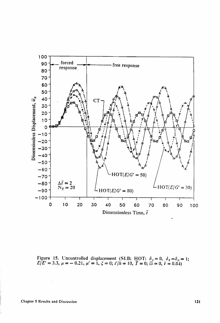
100

90 +

80 -

707

607

50 -

40 -

50 -

20 7

107

| Oo

Oo

‘a

—207

—307

—40 7

—507

—607

-—707

—80 7

—907

Dime

nsio

nles

s Di

spla

ceme

nt,

w,

forced a.

response

free response

At=2 Nr = 20

HOT(E/G’ = 50)

HOT(E/G’ = 80) HOT(E/G’ = 30)

—100

10 20

I

30

I T

40 90 60 70


Figure 15. Uncontrolled displacement (SLB; HOT: 6, E/E’ = 3.3, n= — 0.21, p’ = 1, €=0; Z/h = 10, T=0;


80 90

100

121

100

forced

response 90 L,___

807

707

60-

507

407

307

207

107

-10 * ‘ %

—20-

-—307

~407

-—507

—60- oad yo —-70°7

-—80- Ar=2 @ = 0.05

-90°-

—-100 ] T I T —T —T T T

0 10 20 30 40 50 60 70 80 90 100


«—_________ free response

i

x

pe

As

*

_

|

Dimensionless

Displacement,

wv,

Figure 16. Uncontrolled displacement (SLB: HOT: 6, =6, =06,,= 1; E/E’ =5, E/G’ = 30, § = 0; ?/h = 10, T = 0; v = 0.03)


~*———— forced response free response

GW Oo j

l oO l

Dimensionless

Displacement

l I

W

N

oO Oo

!

! —40 7

-507 HOT(E/G’ = 50)

-60 7

-70 T T ] T T l l

0 10 20 30 40 50 60 70 80 90 100


Figure 17. Uncontrolled displacement (SLB; HOT: 6,=0, 6,=6, = 1; E/E’ =5, ¢ = 0.05; 7/k = 10, T = 0; w = 0.1, ¥ = 0.02)


12

jo ———— forced response f 10-7 ree response

HOT(E/G’ = 50)

Dimensionless

Velocity,

dwv,/dt

\L Hor, oe = 10)

\

-87 _ HOT(E/G’ = 40

At= —107 Ny = 30

—-12 T T l rT T l TT

0 10 20 30 40 50 60 70 80 90 100


Figure 18. Uncontrolled velocity (SLB; see Figure 17)


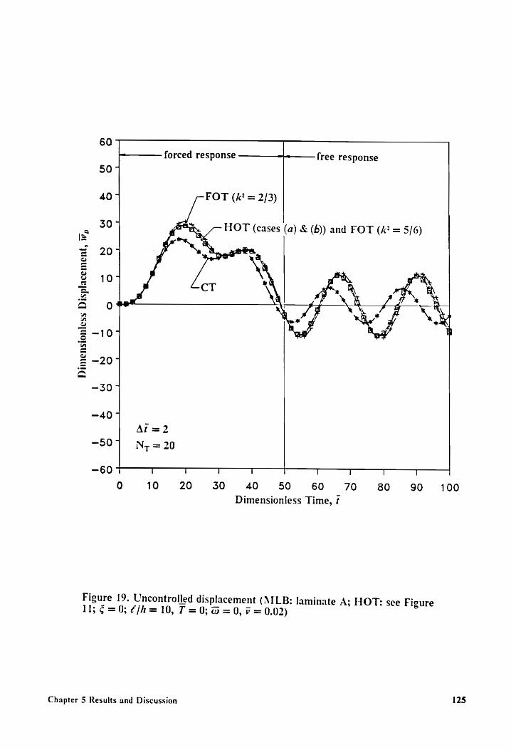
60 forced response

-———free response 507

407 FOT (A? = 2/3) 30° HOT (cases (a) & (6)) and FOT (4? = 5/6)

ae. \ a. BX

Lo: Ke KY MS —207

»Wp

20 -

107

Dimensionless

Displacement

—307

-—407

-50) N,=20

-60 T T T T T T T T

0 10 20 350 40 50 60 70 80 90 100


Figure 19. Uncontrolled displacement (MLB: laminate A; HOT: see Figure 11; ¢ =0; 7/4 = 10, T =0; @ = 0, ¥ = 0.02)


-«—————. forced response free response

FOT (k? = 2/3)

Dimensionless

Velo

city

, dw

,/dt

A? =2 HOT (cases (a) & (6)) and FOT (k? = 5/6)

-S7 N,=20

—6 I T yl

0 10 20 30 40 50 60 70 80 90

100


Figure 20. Uncontrolled velocity (\1LB; see Figure 19)


60

-~-———— forced response te free response 50 7

FOT (4? =2 4 i ( , /3)

A 50 - .

ix = 20- a

= ad

@ 10°

SB oO 2 3-107 E -20- &

—-307

-40 7

At =2

~S07 N,=20

—60 l ! l l I l 0 10 20 30 40 £50 60 70 80 90 100


Figure 21. Uncontrolled displacement (MILB: laminate B; others, see Fig- ure 19)


Dimensionless

Displacement,

iv,

80 79 }~———— forced response free response

607 CT (type A - D laminates)

507 | HOT (type D laminate)

407

i HOT (type B laminate)

—50 7

-601 Ar=2 ‘\ | . -794 Nr =20 HOT i pe C laminate)

—80 T T ! a | ] l

0 10 20 30 #40 = £50 60 70 80 90 100


Figure 22. Uncontrolled displacement (MILB; HOT: 5, =0, 5, =6,= 1; €=0.01; 7/h = 10, T = 0; w = 0.1, » = 0.02)

128 Chapter 5 Results and Discussion

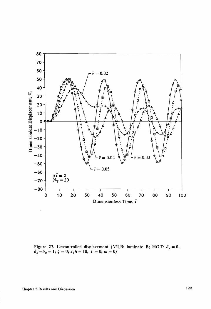
Ny = 20

Tat {uaa UpUSIC]

SSJUOISUIUNG —70-

—80

80 90 100 70 20 50 40 50 60


10

129

; @ =0) = 0 >€=0;¢/h=10, T Figure 23. Uncontrolled displacement (MILB: laminate B; HOT: 6, =0,

6, =0, = 1;


130

oon

” ao?

n

\. >»

\

0.35

- ~o"

-

100 90

0.02; others,

80

v

70

t 60 90

forced response a free response

\

“A a 4 ie -\ ‘ ‘ A

a

=2

Ny; = 20

At

30 40

Dimensionless Time,

20 10

4. Uncontrolled displacement (MILB: laminate B:

5

Pd

“Ty

T Tt

T T

T T

T T

Oo Aa

Oo 0

Oo oO

Oo OO

OO Oo

44 Suauaoypdsiq,

SsajUOIsuaig

oO 0

~—70-

—80

Co TE

Oo oOo

Oo 9

ree ey

see Figure 23) Figure


5.2 Plates without Control

5.2.1 Eigenfrequencies

The eigenfrequencies of a square SLP obtained by using the HOT and CT are

compared in Figures 25-27 for different thickness ratios ?7,/h. The results obtained here

are found to be similar to those of SLB shown in Figures 2-4. In Figure 28, the second

frequency spectra and the shear cut-off frequency of a SLP are illustrated. The results

are found to be similar to those of SLB shown in Figure 6.

Finally, the trend of the eigenfrequencies of plates shown in Figures 27-32 are found

to be similar to those of beams given in Figure 7-10.

5.2.2 Uncontrolled Dynamic Response

The displacements and velocities of a SLP predicted by the CT and HOT are com-

pared in Figures 33 and 34, respectively. It is shown that the responses are greatly

underestimated by the CT. Furthermore, the rotatory inertia as well as the transverse

normal stress are shown to have negligible effect on the responses.

Under the same loading condition, the displacements of a SLP for different aspect

ratios (i.e., 7,/?,) are illustrated in Figures 35-37. The difference between the displace-

ments predicted by the CT and HOT is shown to be affected very much by the aspect

ratio.


> 1

CA l

(¢,/2,= 1, 2,/h=5)

HOT (64 = 53 = 5) = 1), Qimn HOT (6, =0, Op =0n= 1), 2

HOT (6, =6,=0, 6 )

CT, Qqyin

ho 1

Dimensionless

Freq

uenc

y Q,

,,

(or

2,,,

,)

—_ i

(1, 2) and (2, 1) mode

w=), mn

oo

(1, 1) mode 0 T

0 5 10

T

15

[

20

J 1 i / |

25 50 55 40 45 50


Figure 25. Eigenfrequencies (SLP; E/E’ = 5; T, =T, = 0)


2.9

(2, 2) mode (2,/2, = 1, 2,/h = 10)

2.0 - ——_——_ HOT (5, = 5, = 5,= 1), Qin ao} HOT (54 = 0, 5g = 5), = 1), Qinn

-~-——-—— HOT (6, = 6, =0, 5,,= 1), Qian --——--—— _ CT, 2,

lo 1.54 oo «ao == "=o = es

1.0 -

(1, 2) and (2, 1) mode

Dime

nsio

nles

s Frequency

22,,,

(or

2,,,,)

ao On i

(1, 1) mode

0.0 V T T T T I T T T

Q 3 10 15 20 25 $0 35 40 45 £50


Figure 26. Eigenfrequencies (SLP; see Figure 25)


Dimensionless

Freq

uenc

y Q,

,,

(or

Q,,,

,)

1.0

0.8 -

0.4 -

0.25

HOT (5, = 6, = 6, =1),Q {mn

--------. HOT (54 = 0, 5p =5y,= 1), Qin -—————— oe HOT (6,=6,=0, 67 = 1), Qrr

-——--— CT, 2,

Loa 1) mode (7,/2, = 1, 2,/h = 30)

0.0 t | | D ! J { I i

5 10 15 20 25 30 55 40 45


Figure 27. Eigenfrequencies (SLP; see Figure 25)


50

134

100

i a f,[h = 30, Qann --——--— 9 ¢,/h = 30, Q,

_ 80° é,/h = 10, Qsng aa -—-——— ¢,/h = 10,2, = 707

i? 60 4 = 2, 2) mode

= 50 4

2 (1, 2) and (2, 1) mode % 40-7

= 304 = (1, 1) mode

Os a es *Sseesiiiiiiiisicsi:::'

107

Q l I 0 5 10 15 20 25 30 55 40 45 50


Figure 28. Second frequency spectra (SLP; E/E’ =5; 0,/?,= 1, T, = T, = 0)


> L

Dime

nsio

nles

s Fr

eque

ncy,

2,

(or

,,,,

)

’ «oe

GA l

(2, 2)

N i

_ 1

;

oS

HOT (54 = 5g = 51, = 1), Qin HOT (6,=0, 6,=6, = 1), Q,, FOT (k? = 5/6), Q,,, FOT (k? = 2/3), 2, CT, 2,,

mode

1, 2) and (2, 1) mode

(1, 1) mode

—

4 if i if l t tC

5 10 15 20 25 30 35 40 45 50

Length to Thickness Ratio, 7,//

Figure 29. Eigenfrequencies (MLP: laminate B; 7,/7,= 1, T, = T, = 0)


Dimensionless

Frequency

22,

~

1- So ~

Laminate A, HOT -----~~- - Laminate B, HOT -—-— Laminate C, HOT -—— --—— Laminate A - C, CT

(7,/0, = 1)

2, 2) mode

(1, 2) and (2, 1) mode

(1, 1) mode

20 25 30 35 40 45 50

Length to Thickness Ratio, 7,/h

Figure 30. Eigenfrequencies (MLP; HOT: 6, = 0, 6, =0, = 1; T, =T, = 0)


T, = T, = 10, HOT be nnn T, = T, =0, HOT ‘

es oe ee T, = T, = —4, HOT 44\ --——---—— F,=7,=10,CT

| \ a ‘ (7,/?,= 1)

234 \ z \\ \ & \ \

= \ . (2, 2) mode Sati \ \ 2 = (1, 2) and (2, 1) mode

(1, 1) mode

Length to Thickness Ratio, 7,/h

Figure 31. Eigenfrequencies (NILP: laminate B; HOT: 6, = 0, 6, =6,,= 1)


Dimensionless

Freq

uenc

y,

Q,,,

, (o

r Q)

)

45

pb Oo i

GW

on i

GW Oo 1

nO

on L

nh © 1

on 1

OQ !

on 1

Laminate A, Qynn -——-— Laminate A, Q,

(1, 2) and (2, 1) mode

. (1, 1) mode

oo nnnn ne. Laminate B, Quinn e , “2 Z -——--—- Laminate B, Q, Op te

(,/2, = 1) ee oe

oo”

Yo

fo

fo wee

7 - ore . . a

‘ i J I { | J t

S 10 1S 20 25 50 35 40 45

Length to Thickness Ratio, ?,/h

Figure 32. Second frequency spectra (NILP; see Figure 30)


50

139

50

<< forced —}»t_— free response response

40 -

30 -

207 CT

104

0 \ lh <2 — TT ~ wo ~

—40 - - [ At=2 HOT: cases (a) — (c) Ny(m = 5,2 =5) = 25

-

I oO i

Dimensionless

Displacement,

iv,

i N a 1

! W oO i

-S0 | ! | 4 an | 4 | { 1

0 10 20 50 40 90 60 70 80 90 100


Figure 33. Uncontrolled displacement (SLP; HOT: (a) 6,=6,=6,,= 1, (b) 0, =0, 6, =0, = 1, (c) 0, = 6,= 0, 6, = ls E/E’ =5, E/G’ = 50, & = 0; f,/h = 10, 7,/?, = 1, T= T, = 0; @ = 0.2, v = 0.04)


20

forced __ylg free response response

15-

| 107 CT

Ss = A\ . \ L.. 4 = fs 4 - a = 9 | | \- TI ORES ST

z —5 4

2 5

-10-

-157

At=2 N-(m = 5, = 5) = 25 HOT: cases (a) — (c) -~20 ' | : | T T rT T —

0 10 20 50 40 50 60 70 30 90 100


Figure 34. Uncontrolled velocity (SLP; see Figure 33)


70 j<—— forced response ——_—_ ag —— free response

Dime

nsio

nles

s Di

spla

ceme

nt,

w,

| I

1 GQ

nN

=

Co 0

0 0

Ll 1

i

| |

oO op

Oo Oo

1 L

{ nv

Oo 1

- C,/0,= 1 -707 At=2 fi /h= 10

-80 i i | oT t tO | I

0 10 20 30 40 50 60 70 80 90 100


Figure 35. Uncontrolled_displacement (SLP; HOT: 6,=0, 6,=6, = 1; E/E’ =5, ¢ = 0.05; 7, = T, = 0; @ = 0.25, v = 0.02)


Ca

oO

“<——— forced response free response

a

ws oa

o

1 t

- HOT(E/G’ = 60) | an

oO

i | i \ HOT(E/G’ = 40) bh oO i

» Wp |

HOT(E/G’ = 20) A © i =e

we

.

o

—_—

—-

N

oO

oO l

1

1 oOo oO

1

=

Dime

nsio

nles

s Di

spla

ceme

nt

Ar= é,/h = 10

rs

es

; ot

N DO

OO

PRP WN

90 0

9009

0 0

i 1

i 1

i i

I 0 oO

‘ } q \

0 10 20 50 40 SO 60 70 80 990 100

Dimensionless Time, tf

Figure 36. Uncontrolled displacement (SLP; see Figure 35)


80

70 5

60 -

50

40 -

—f—__—_— forced response

—~

N

Gi

Oo oO

Oo

l

l i

free response

HOT(E/G’ = 60)

HOT(E/G’ = 40)

{ Oo

Oo 1

Dimensionless

Displacement,

iv,

Ar=2 NrUn = 5,2 = 5) =25

rr

en rs

VY Oo

OW

RF

WwW

BN o

Oo 00

90 0

1 i

i 1

i i

HOT(E/G’ = 20)

,/0,=2 f {hk = 10

I ©a

o

| T I

10 20 50 o

—T !

80 90

{ 1 t

40 30 60 70


Figure 37. Uncontrolled displacement (SLP; see Figure 35)


100

144

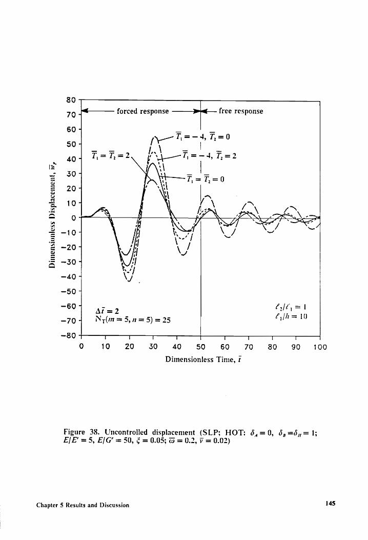
oa

oO

“<—_—_———- forced response free response

70 - 60 - 50 -

_ 404 = 30- 2 207 2 10; Eo 2 -10-

5 2

{ (

I l

t a

oO BP

Ws

N

mo Oo

A

AO OA

i

! 1

l l

- C,/¢, = l

Ar =2 =) _ ye éi[h = 10 —-704 Nyrln=5,n = 5) = 25

—80 T T T T T T tT

0 10 20 40 50 60 79 80 90


100

Figure 38. Uncontrolled displacement (SLP; HOT: 6,=0, 5,=6,= 1; E/E’ =5, E/G’ = 50, ¢ = 0.05; @ = 0.2, vy = 0.02)


60

90 5 > = 0.04

40 5 7 = 0.03 i

i 30 y= 0.02

= 20- 2

2 AAA AY 5 Oo SAA | x

o

= -20 4 7 = 0.05 5

~30 -

-40 +

At = 2 C,/0, = 1 Oy fh = 10 —60 1 I i ! l { \

0 10 20 30 40 30 60 70 80 90 100


Figure 39. Uncontrolled displacement (SLP; HOT: 5,=0, 6, =), = 1; E/E’ =5, E/G’ = 50, € =0; T,= T, = 0; @ = 0)


100

“<— forced response 3>—€— free response

80 +

60 - @=0 w@ = 0.25

wo =0.2

= 407

5 20 5

- 0

= -20-

S = —40 5

—60 5 o=0.1

—80- Ar=2 0,/?,=1 N =5,n=5)=25 2h = 10 (im = 5,n = 5) = 25

-100 T r r 0 10 20 30 40 #=.‘$S0- 60 70 80 890

Figure 40. Uncontrolled displacement (SLP; HOT: 6,=0, 6,=6, = 1; E/E’ =5, E/G’ = 50, é = 0; 7,



= T,=0; 7 = 0.03)

147

120 —<¢————. forced response —_ pe free response

100 -

39, (@ = 0.3) ‘\

Oo

I No Oo

I b oO

Dimensionless

Displacement,

i,

-—60-

—80 7

-1007 Ar=2 HOT (cases a & b)

Ny(m = 3,n = 5) = 25 and FOT (A° = 5/6)

-120 r T T T ] ] T

0 10 20 350 40 50 60 70 80 90 100


Figure 41. Uncontrolled displacement (\ILP: laminate B; HOT: see Figure 33; § =0; 7, = 7, = 0; @ = 0.3, v = 0.02)


100

“——— forced response —-——_ag— free response

80 5

60 -

= 404 A 5 / \ /\ = | [ \ g 207

{ \

7 [is /N So 0 t~ —- —

z | \ | \ = 4 | | = ~20°7 \ | |

g Vy — Vv J 5 -40-

HOT (cases a & b)

—60 - and FOT (k* = 3/6)

—-80 75

-100 l T T T ! ! l 0 10 20 50 40 50 60 70 80 90 100


Figure 42. Uncontrolled displacement (NILP: laminate B; see Figure 41)


Dimensionless

Displacement,

wp

50

“{——— forced response ae free response

40 -

(@ = 0.1)

305

FOT (4? = 2/3) 20 5 CT

10 -

“ “ ~~ 7

0 [St \ HM dicches iS \7 \7%

— | QO “4

HOT (cases a & b)

-20 5 and FOT (k” = 5/6)

—30 ~

“407 Ar = 2 ,/¢,=1 NyQn = 5,2 = 5) = 25 fi /h= 10

-50 1 t J J q if i 1

0 10 20 30 40 30 60 70 80 90 £100


Figure 43. Uncontrolled displacement (NILP: laminate B; see Figure 41)


50 “—__—— forced response -——_y>mq— free response

40 - (ow = 0) /\ FOT (A? = 2/3)

Yn

. He \\ Is / = 20° rc \ z , \

3 10> L\ TN LS™ = — =~ \ om \ ™~ /N

Ag _ WA A\ \ gs \ / NY / / 2 CT / \ = -10;7

2 HOT (cases a & b)

& -20- and FOT (k? = 5/6)

—30 4

—40 - At= f,/C,=1 Nr(n = 5, =5) = 25 2h = 10

-—50 T T T r TT !

0 10 20 50 40 20 60 70 80 90 100


Figure 44. Uncontrolled displacement (MILP: laminate B; see Figure 41)

Chapter 5 Results and Discussion 1S1

60

mg@— forced response ple free response

50 - | 40 - HOT (Laminate C)

rn oe 30- Nan HOT (Laminate B)

i 204 ‘ CT ( Laminate A - D )

Oo t

I Oo ©

l !

Dimensionless

Displacement,

wv,

20" \ HOT (Laminate D)

| ~S0° \ hs HOT (Laminate A)

ti! -40 7 Ww V/

-S07 Ar=2 (2/7, =1 Nr(m = 5,2 = 5) = 25 f,/h = 10

—60 l ! I

Q 10 20 50 40 50 60 79 80 90 100


|

Figure _45. Uncontrolled displacement (MLP; HOT: 6,=6,=6,= 1; é = T,=0; ® = 0.2, ¥ = 0.03)


The effect of different combinations of edge loads on the displacement of a square

SLP is illustrated in Figure 38. The displacement is determined based on the HOT. The

influence of the travelling velocity and forcing frequency of the external load are shown

in Figures 39 and 40 , respectively. In both cases, the displacement is obtained from the

HOT.

The displacements of a MLP (laminate B) obtained by using the CT, FOT and HOT

are compared in Figures 41-44 for different forcing frequencies of the travelling load.

In Figure 45, the displacement of four different laminates determined from the CT and

HOT are compared. The same trend as in the case of MLB is observed.

In the following, the control problems are considered.

The performance index which 1s chosen to be minimized is described in Chapter 4.

For convenience, it is repeated here. For the CMC approach, it is defined as

7-41] (a, Qty +2’ R,2) dt 0

where

_ _ _- T Uy = (4; 99 Ins Ty oo Qn)

_ — ~

Z= (a), vee yg ayy Mm, ceey my)"

The state weighting matrix Q is chosen as

Q A, O

| O A,

where


A, = diag{qy, Qi, tees FunS2n}

A, = diag{ yy, rong Fwnt

in which q,, are weighting parameters for states. For the IMSC approach, one has

| (Uy Quy +f R,f,) df 0

where

The control input weighting matrix is chosen as

R, = diag{ryy, + Twn}

where r,, are weighting parameters for control inputs. The performance index in this

case could also be expressed as [1,2]

- - - 41f - j=) 4, =>] (¥, Q,¥, + typ fr) dt

where

According to Eqs. (4.3.3), the modal control inputs f, are related to the physical

control inputs z by


where

B,, = [Bai Bia]

in which B,, and B,, are given by Eqs. (4.3.5b).

It can be seen that if the number of actuators and controlled modes are the same,

and if the control input weighting matrices in the CMC and IMSC approaches are re-

lated by

R.=B, R,B,

the performance indices obtained from both methods are identical. This condition was

derived by Meirovitch et al. [2].

For simplicity, in numerical examples the weighting parameters q,, are taken to be

1 and r,, are assumed to be the same for all the controlled modes. Furthermore, the

dimensionless cost kernel C; is defined as follows:

= l ~ = - Cr= > (Uy Qily +2” R,Z,)

for the CMC approach, while

n _ 1 _

Cr= a DF QT, + rr f)

for the IMSC approach.

The following dimensionless quantities are also used:


SLB:

an= a, a=

ars Elf ELny EL hy j,=- if) 7x 10%, c= i) Ex 10°

0 Po

MLB:

= D,h = = a ap= a, a= 2

Pot D,h

= ( (Dyhy x 10° TD = Crx

eo

SLP:

= 10 (1. hw Eh’ = ap = — (- ) o a oan) ee?) Po

= f, ¢ ~ a=12%1—p’y(— + yr ( \( 2, (F-) Ee

= Cr ti > hw E*h* 5 Cry = ———— (—)'( — * —_ «x 10 7 taal — wy 6 e,) pe

MLP:

= _ 10Dh = =_ fit, ~ ~ pol it 0, ° Dh

_ Diy oH p, 10°

(Po? 1¢2)

Next, the numerical results concerning the control of beams are discussed.


5.3 Beams with Control

5.3.1 Closed-Loop Poles

In Figures 46-49, the effects of the modelling error due to the use of the CT and the

variation of material properties on closed-loop poles are illustrated. Here, the CMC

approach with a diagonal control input weighting matrix and having the same number

of actuators and controlled modes is considered.

In Figure 46, both nominal (CT) and actual (HOT) plants have included the

damping (€ =0.1). It is found that both the stability margin (which is defined as the

horizontal distance from pole location to the imaginary axis) and the stiffness (which is

defined as the distance between the location of the pole and the origin of the axes) of the

actual system are smaller than those originally designed (by using the nominal plant).

The difference is shown to increase as the E/G’ ratio associated with the actual system

becomes larger.

It is shown in Figure 47 that when damping is neglected in both nominal and actual

plants, the stability margin remains unaffected, while there is a significant decrease in the

stiffness of the actual system compared with the nominal one. Since damping always

exists in the actual plant, the pole locations shown in Figure 47 at best could only be

regarded as those that will be obtained from the limiting case of the real system. If one

includes a certain amount of damping in the actual plant, while neglecting it in the

nominal plant, it is shown in Figure 48 that the stability margin of the actual plant be-

comes greater than that originally designed. However, the stiffness of the actual system

is still found to be smaller than that of the nominal one.


In Figure 49, both nominal and actual plants are modelled by using the HOT. It

is shown that if the E/G’ ratio of the actual plant is smaller than that selected for the

nominal plant, the stability margin as well as stiffness of the actual system could be

greater than those originally designed. In view of this result and that shown in Figure

48, It seems that if the damping is neglected and the largest possible E/G’ ratio is se-

lected in the nominal plant, the resulting control system will be more robust than those

considered in Figures 46-49.

In figures 50-58, the IMSC approach is employed. The results shown in these fig-

ures are similar to those of Figures 46-49 obtained from the CMC approach. The in-

fluence of modelling errors on the closed-loop poles locations for different 7/A ratios is

illustrated in Figures 50-51. The modelling errors being considered seem have less effect

on beams of higher 7/A ratios. The example considered in Figure 53 is the same as that

of Figure 52 except that the transverse normal stress is neglected here (i.e., 6, =0). One

observes that the effect of transverse normal stress could be ignored.


3.0

4 3rd mod 2.5 ilk = 10 rd mode—9s

2.0 - o\ E/G’=10 o

» 1.57 re 2

& 1.07 2nd mode -® c. . \ 100

5 a, 0.57

2 Ist mode —@

O 0.0 S g

E -9.571 © nominal plant (CT) rm x Ist mode

s -1.0- A 2nd mod actual plant = O 3rd mode | (HOT)

= —-1.57 Oo = o

D -—2.07

-—2.57 9

—-3.0 T T Tr T I

—1.2 -1.0 -0.8 -0.6 —0.4 —0.2 0.0

Real Part of Closed-Loop Poles

0.2

Figure 46. Closed-loop poles (SLB; HOT: 6,=0, 6,=6,=1; E/E’ =§, ¢ =0.1; T=0; CMIC: R, =r, 1, r, = 10, 3 force actuators at x = 0.25, 0.5, 0.75)


3.0

4 3rd mode ——e 2.5 ifh = 10

2.07 ao) E/G’ =10 o

2 1.57 5

. 1.07 2nd mode

= " _

Ss 05-4 | a . Ist mode G Ry

= 0.0 = y ae —_ 7

S 0.5 © nominal plant (CT) a * Ist mode tual plant = -1.07 A 2nd mode (HOD. an e © 3rd mode

= -1.57 a QO Q

—2.07

—2.57 e

-3.0 l T ! I !

—1.2 —1.0 —0.8 —0.6 —0.4 —0.2 0.0 0.2


Figure 47. Closed-loop poles (SLB; ¢ = 0; others, see Figure 46)


3.0

2.5 7 a= 10 3rd mode-®

2.0 ~ 5 E/G’ = 10

o

1.57 Q

o—2nd mode 1.07

\ 100

0.57 \ae— Ist mode

Imag

inar

y Pa

rt

of Cl

osed

-Loo

p Po

les

0.0

He

—O8.57 © nominal plant (CT, ¢ = 0)

-1.07 A 2nd mode actual plant

O 3rd mode | (HOT, ¢ =9.1) °

-1.57 a

oO —-2.07

—2.5 7 °

-3.0 i T —T | ]

-1.2 -1.0 -08 -06 -0.4 -0.2 0.0 0.2 Real Part of Closed-Loop Poles

Figure 48. Closed-loop poles (SLB; see Figure 46)


3.0

25°1 k= 10

2.07 o \ E/G’=10 o

S 1.57 q o & 1.07 3rd mode 100

= \ 2nd mode 3S 0.57

S Ist mode—*\ = 0.0 = *

& —9.57 © nominal plant (HOT, E/G’ = 50) > * Ist mode actual! S -1.07 4 2nd mode (HOD i) O 3rd mode

= -1.5- o Q

a —2.07

—2.57

-3.0 ] ] r— T I

—1.2 —1.0 —0.8 —0.6 —0.4 —0.2 0.0 0.2 Real Part of Closed-Loop Poles



7

6 - 3rd mode

Yh=4 5 ~

4 47 3 n\ EIG =5 e s § 2nd mode—* 4, S :

J 25 Ay = rN 5 1 Ist mode \ 100

= 0 c f E. f o © nominal plant (CT) {9 = 9+ x Ist mode t 1 A

‘So 2 A 2nd ma (HOD. ant o = 34 O 3rd mode 3 = Q

—4 7

-5-+

—67 °

-7 T ! ] ! l

—1.5 —1.2 —0.9 —0.6 —0.3 0.0 0.3


Figure 50. Closed-loop poles (SLB; HOT: 6,=0, 6,=6, = 1; E/E’ =5, ¢ =0.05; T = 0; INISC: r, = 10 )


2.0

1.57 lh =20

3rd mode E|G’ =5

, 1.0" = i)

un 100 = 2nd mode ¢ 4 5 08 “A =

Qo

zs Ist mode —g, O 0.0 Come 8

cS

c. -0.5- © nominal plant (CT) }

pT * Ist mode | actual plant cs A 2nd mode (HOT) = O 3rd mode

= 1.07

9

-1.57

—2.0 ] l l —T

—1.5 —1.2 —0.9 —0.6 -0.3 0.0 0.3



164 Chapter 5 Results and Discussion

3.0

4 3rd mode-o 2.5 Ih = 10

4 O \E/G’ =5 2.0 oO

os Oo

2 1.57 a a ss | 2nd mode-® 8 1.0 v 100

z 0.57 S Ist mode—@\

= 0.0 2 g

< —9-5) © nominal plant (CT)

= 0 3rd mode | (HOT)

| S7 Oo oO

—2.07 " ao

—2.5 7 °

-3.0 T —T r T

—-1.5 —1.2 -0.9 —-0.6 —0.3 0.0

Figure 52. Closed-loop poles (SLB; HOT: 6, =0, 6, =6, = 1; E/E’ = 10,


€=0.1; T= 0; IMSC: r, = 10 )


3.0

4 3rd mode —e 2.5 I[h = 10

a\ E/G’=5 2.0 7 o

oO 1.57

”“ 1.07 2nd mode 3h 2 . * 100

= 057 S Ist mode —e,

: 0.0 3

= 9-57 6 nominal plant (CT)

2 1.07 A dnote rer Pan : a O 3rd mode | (HOT) °

= -1.57 OG a QO

—2.0 4

—2.57 °

—-3.0 T T T T

—1.5 —1.2 -0.9 —0.6 —0.3 0.0 0.3


Figure 53. Closed-loop poles (SLB; HOT: 6,=6,=0, 6,= 1; others, see Figure 52)


3.0

4 3rd mode-© 2.5 ih = 10 o\ E/G=5 2.0 7 4

o 2 1.57

a. 2nd mode-a\a 1100

2 1.07 *\ —

> 2 0.57 s °° \

CO Ist mode-® S 0.0

a -0.57 . - , > . © nominal plant (CT, T = 0) g * Ist mode

‘Sy ~-1.07 A 2nd mode actual plant f S O 3rd mode | (HOT, T = 10)

™ =1.55

Oo -—2.07 Oo

a

—2.5 7 °

—3.0 T T T J T

-1.5 —1.2 -0.9 -—0.6 -0.3 0.0 0.3


Figure 54. Closed-loop poles (SLB; HOT: 6,=6,=0, 6,= 1; others, see Figure 52)


3.0

a 3rd mode-o 2.5 lh =10

2.0- o\ E/G’=5

oO

: 1.57 oD

c. 2nd mode—o Ss 1.07 \ ml = \ 100 9 0.57 © o ist mode—q

‘<= 0.0 S 3 & -0.5- _ > © nominal plant (CT, T =0) aq * Ist mode = 71.07 A 2nd mode actual plant 6 g O 3rd mode | (HOT, T =—3)

= 15> B Qo

~—2.0 7 o

—2.5 7 9

—3.0 l T T l

—-1.5 —1.2 —0.9 —0.6 —0.3 0.0 0.3


Figure 55. Closed-loop poles (SLB; HOT: 6,=6,=0, 6, = 1; others, see Figure 52)


3.0

2.5- th = 10 3rd mode—®

4 Qa {E/G’=5 2.0 4

7) Oo a o 3 1.5

oe J 2nd mode § 1.0 100

2 os: = lst mode —4;

‘ss 0.0 " |

> —0.5 7 © nominal plant (CT)

B-1.07 A Bile |atul ta g QO 3rd mode (HOT)

= -1.5- O o

o —2.07 0

-2.57 °

—3.0 T T yl T

-1.5 —-1.2 -0.9 -—0.6 -0.3 0.0 0.3


Figure 56. Closed-loop poles (SLB; HOT: 6, =5, = 0, 5,,= 1; € = 0; others, see Figure 52)


3.0

| 3rd mode—o 2.5 ih = 10 r

2.07 vo E/G’ =5 wn oO

2 1.57 - qoand mode

8 1.0 \ 100

x 2 0.57 5 wets: mode

= 0.0 : a,

= 79-57) © nominal plant (CT, € = 0) a * Ist mode = -1.0} A 2nd mode | ‘OT plant e O 3rd mode | (HOT, ¢ = 0.1) e = 1,57 a

oO

—2.07 4

—2.57 °

-—3.0 T T —T T

-1.5 1.2 -0.9 -0.6 -0.3 0.0 0.3 Real Part of Closed-Loop Poles

Figure 57. Closed-loop poles (SLB; HOT: 6, =6,=0, 6, = 1; others, see Figure 52)


3.5

© nominal plant (CT) 4 actual plant (HOT, type A laminate)

$3.07 x actual plant (HOT, type B laminate)

\ 2.5- (yh = 10} 820 0 00000 oO CGERGE

r, = 2.5 ——————_ r= 10

AA A &bL444 4 OAs 2

n

eg

o a

aq So °o

ml

ws 2.0- 3 2 3rd mode

v OA ASSAM) 4 Avena °o

t 1.5- i-4

a

c 6S Gece ccm =

= 1.0 2nd mode

ek Ok OR RE Oe INE REE

0.5 -

Ist mode _[S=3 2 2 29S 9 22s

0.0 T ! ! I —1.0 —0.8 —0.6 —0.4 —0.2 0.0 0.2


Figure 58. Closed-loop poles (MILB; HOT: 6, =6, =0, 6,,= 1; € = 0.005; INISC)


Besides the type of modelling errors already considered, the omission of the edge

load in the model could also have a stabilizing or destabilizing effect on the control

system. This is illustrated in Figures 54 and 55. It is shown that the neglect of the ex-

isting tensile load in the nominal plant has a beneficial effect, while if it is a compressive

edge, by neglecting it in the nominal plant the performance of the control system could

deteriorate. In Figures 56 and 57, the effect of damping is illustrated. Finally, in Figure

58 the closed-loop poles of two MLB (laminates A and B) are compared. The modelling

error seems to have a greater influence on the closed-loop poles associated with the

laminate B.

5.3.2 Controlled Dynamic Response

In Figures 59-65, the control of SLB by the CMC approach is considered.

The controlled displacements and velocities of nominal and actual plants compared

with those of the uncontrolled actual plant are shown in Figures 59 and 60, respectively.

It is found that the controlled responses are underestimated by the nominal plant which

is modelled based on the CT. The difference between the actual and nominal controlled

responses, however, diminishes very quickly as soon as the travelling load leaves the

structure. It is also illustrated here that the vibration amplitude could be reduced sig-

nificantly during the forcing period (i.e., while the travelling load is still acting on the

structure) by choosing proper feedback gains.

In Figures 61 and 62, the effect of the control input weighting parameter r, on the

controlled response is Ulustrated. When a relatively large r, is chosen, the resulting

feedback gain could be so small that the control loses its effect as indicated in Figure 62.

The controlled responses shown in Figure 63, although using fewer actuators, do not


differ too much from those of Figure 61 where the number of actuators is chosen to be

the same as that of controlled modes. The reason for this could be that the actuators

used in the example of Figure 63 are placed at the same effective locations on the beam

(especially the one located in the middle) as those in Figure 61. This, however, does not

mean that using fewer actuators is a better choice, since as will be shown later the

magnitudes of the actuator output in this case are higher.

In contrast to the case considered in Figure 63, both force and torque actuators are

used in the examples of Figures 64 and 65. It is shown that the difference between the

controlled nominal and actual plants becomes larger. An explanation of obtaining such

a result is that the torque actuator is more effective in bending the stiffer structure,

which is the case of the nominal plant modelled by the CT.

In Figures 66-72, the control of SLB by the IMSC approach is considered.

The displacements and velocities of the uncontrolled actual plant, controlled nomi-

nal and actual plants are compared in Figures 66 and 67, respectively. The effect of the

control input weighting parameter rv, on the controlled response is illustrated in Figures

68-72. It is found that when a relatively small 7, is chosen (which results in large feed-

back gains), the difference between the controlled nominal and actual plants disappears

as shown in Figures 68 and 69. In practice, however, the use of high feedback gains is

not always possible, which could be due to, for example, the constraints on control

hardwares or the stability problem related to unmodelled dynamics. In the other ex-

treme, if a very large r, is chosen, the controlled system virtually can be regarded as an

uncontrolled one as illustrated in Figure 72.

In Figures 73-76, the control of MLB by the CMC approach is considered.


70

60 SS with the moving load ———=-—— without the moving load

50 7

40-7 nominal plant: CT actual plant: HOT

307

207

-10°7 —20-

Dimensionless

Displacement,

w,

—30 7

controlled (actual plant)

-—40 7

-507 |- At=2 uncontrolled (actual plant)

-6o7 Nr=> N,=5

-70 —T T T_ T T— r l

0 10 20 30 40 50 60 70 80 90 £100

Dimensionless Time, t

Figure 59. Controlled and uncontrolled displacements (SLB; HOT: 6 6,=0,=1; E/E’ =5, E/G’=50, €=0.05; ¢/h=10, T=0; @ v= 0.02; CMC: R,=r, I, r, = 10~, 5 force actuators at x = 0.1, 0.25, 0.75, 0.9)


12 -—— with the moving load ———~~——- without the moving load

107

8°) nominal plant: CT 5 actual plant: HOT

4-

Dime

nsio

nles

s ve

loci

ty,

div,

/0t

controlled (nominal plant)


At=2 ~107 Nr =5 uncontrolled (actual plant)

=5 —-12 T T T l T T T T

0 10 20 30 40 50 60 70 80 90 100


Figure 60. Controlled and uncontrolled velocities (SLB; see Figure 59)


120 ~—__——— with the moving load

100-7 controlled (actual

1 lant 80 nominal plant: CT plan )

actual plant: HOT

607

40 -

207 "

Dimensionless

Disp

lace

ment

, w,

—407

—607

uncontrolled

80) tual plant

= controlled (nominal (actual plant)

Ar=2 plant) —1007 Nr =)

N,=5

—120 I , |


Figure 61. Controlled and uncontrolled displacements (SLB; HOT: 6, = 0, 6,=6,=1; E/E’ =5, E/G’=50, €=0.1; 2/h=10, T=0; D=0.2, vy = 0.01; CMIC: R, =r, 1, r, = 10-, 5 force actuators at x = 0.1, 0.25, 0.5, 0.75, 0.9)


120

~—_————— with the moving load - 1007

| _— controlled (actual

80 nominal plant: CT plant) actual plant: HOT

607

I= <= 407 2 =

>

a 207 k = 4

= O saqets,, fF

g

2-407 =

-—607

—&0 5 -_ 4 uncontrolled

At=2 controlled (nominal (actual plant) -1007 Np=5 plant)

N,=5

—-120 I T T I I 0 20 40 60 80 100 120

Dimensionless Time, 7

Figure 62. Controlled and uncontrolled displacements (SLB; CMC: r, = 10-75 others, see Figure 61)


120

Pe with the moving load 1007

controlled (actual 7 lant

80 nominal plant: CT plant) | actual plant: HOT

60

= |

= 40

= 2 207 ms a etn = O caea2te,, f, A ,

"2 -207

2-407 5

—60 7

—807 : uncontrolled

At =2 nlant) led (nominal (actual plant) —1007 T=)

N,=5

-120 I T T

0 20 40 60 80 100 120 Dimensionless Time, f

Figure 63. Controlled and uncontrolled displacements (SLB; CMC: 3 force actuators at x = 0.25, 0.5, 0.75; others, see Figure 61)


120

;>—————_ with the moving load 100 -

8071 nominal plant: CT actual plant: HOT

60 -

Dimensionless

Displacement,

w,

controlled |setuat plant)

i

es ¥

raF

-40 7

—-60-

~807 ~ uncontrolled Atr=2 controlled (nominal (actual plant)

-1007 Nr=5 plant) N.=5

-120 I T T T

0 20 40 60 80 100 Dimensionless Time, t¢

Figure 64. Controlled and uncontrolled displacements (SLB; CMC: 3 torque actuators at x = 0.0, 0.5, 1.0; others, see Figure 61)


120

179

120

with the moving load

1007


80°) nominal plant: CT actual plant: HOT

607

Dime

nsio

nles

s Di

spla

ceme

nt,

wp

—80- ; uncontrolled Ar=2 controlled (nominal (actual plant) -1007} Nr=5 plant)

N.=5 -120 I T !

0 20 40 60 80 100 120 Dimensionless Time, t

Figure 65. Controlled and uncontrolled displacements (SLB; CMC: | force actuator at x = 0.5 & 2 torque actuators at x = 0.1, 1.0; others, see Figure 61)


70

6077 With the moving load ———>-— without the moving load

507

407 nominal plant: CT 307 actual plant: HOT

207

7 107 Be

Dimensionless

Displacement,

w,

oO

—40- controlled (actual plant)

uncontrolled (actual plant) —70 T T T T T T T T

0 10 20 30 40 50 60 70 80 90 100


Figure 66. Controlled and uncontrolled displacements (SLB; HOT: 6, = 0, 6,=0,=1; E/E’ =5, E/G’=50, §€=0.05; ¢/h=10, T=0; w=0.1, v = 0.02; IMNSC: r, = 100)


12

10 -

87

~—— with the moving load =

nominal plant: CT 67) actual plant: HOT

without the moving load

Dimensionless

velo

city

, 0w

,/Od

t



—107 uncontrolled (actual plant)

-12 l | TT l l 0 10 20 30 40 50 60 70 80 8690

66)



100

Figure 67. Controlled and uncontrolled velocities (SLB; others, see Figure

182

120

100 re with the moving load

80" nominal plant: CT, ¢ =0 60 - actual plant: HOT, ¢ = 0.1

Fy ~ 407 2 =

>

8 207 3

z Oo 0 ¢ a a eS

n

3} ‘e -207 | 2

zg“ QO

S

-60-

g uncontrolled —80 _ . S / (actual plant)

af =< controlled (nominal -1007 i‘1T=> and actual plant)

N,=5

—120 ] l T l T—

0 20 40 60 80 100 120 Dimensionless Time, ¢

Figure 68. Controlled and uncontrolled displacements (SLB; HOT: 6, = 0, 6,=0,=1; E/E’ =5, E/G’=50; ?/h=10, T=0; o=0.2, v =0.01; IMSC: r, = 1.0)


120

1007

807

oO

© !

Dime

nsio

nles

s Displacement,

iv,

with the moving load

plant) controlled (actual

sof

nominal plant: CT, € =0 actual plant: HOT, € = 0.1

4 or

~407

—-60 uncontrolled

20. (actual plant)

Ar=2 | controlled (nominal

-1007 N;=5 plant) N,=5

—-120 T T ] 0 20 40 60 80 100 120


Figure 69. Controlled and uncontrolled displacements (SLB; IMSC: r, = 10; others, see Figure 68)


120

—__—_—_—___— with the moving load

1007

controlled (actual 80- lant)

nominal plant: CT, € =0 P 60 - actual plant: HOT, ¢ = 0.1

40-

20-7

Dimensionless

Displacement,

iv,

fo)

—-207

-407

-607

uncontrolled -~80-4 (actual plant)

Ar=2 |_ controlled (nominal —1007 Nr=5 plant)

N.=5

—-120 T l T TT T

0 20 40 60 80 100 120 Dimensionless Time, ¢

Figure 70. Controlled and uncontrolled displacements (SLB; IMSC: r, = 100; others, see Figure 68)


120

= with the moving load ~

1007 controlled (actual

80 - plant) nominal plant: CT, € =0

actual plant: HOT, ¢€ = 0.1 60 -

FS w 407 <& = >

S 20° A & ; eo,

Zz 0 A :

a = ~20- 2

@ —40-

a -607

-807 }

Ar=2 controlled (nominal uncontrolled

-1007 Nr=5 plant) (actual plant)

N.=5

~120 I T T T T

0 20 40 60 80 100 120


Figure 71. Controlled and uncontrolled displacements (SLB; INISC: r, = 10°; others, see Figure 68)


120

-————— with the moving load 1007

8071 nominal plant: CT, € =0

actual plant: HOT, € = 0.1 _ 607

I>

5 407 4

3 A a 207 \ a

2

a 0 4 y [ A wn \

Z 4 { 5S -207 <

2 A

&

-—607

| controlled and —80 uncontrolled

Ar=2 ~ controlled (nominal (actual plant) -1007 Ny=5 plant)

N,=5

—120 I T l T

0 20 40 60 80 100 120

Dimensionless Time, ft

Figure 72. Controlled and uncontrolled displacements (SLB; IMSC: r, = 10°; others, see Figure 68)


70

60 +*— With the moving load ———>— without the moving load

50 nominal plant: CT

404 actual plant: (a) HOT, (b) FOT (k? = 5/6), (c) FOT (k? = 2/3

Iz 307

S 20- 9 @ 10- = = S 0 ~ a

g = —107 = 5 —-20- & A -30 5 N— controlled (nominal plant)

—40 4 controlled (actual plant (a) & (b)) |

—501 Ar=2 controlled (actual plant (c)) Ny =5 |

-607 N,=5 uncontrolled (actual plant (a))

-70 I [ IT — 0 10 20 30 40 50 60 70 80 90

Figure 73. Controlled and uncontrolled displacements (M{LB: Laminate B: HOT: 6,=0, 6,=06,=1; §=0.01; ¢/h= 10, T=0; O=0.1, ¥ = 0.02; CMC: R. =r, I, r, = 10, 5 force actuators at x =0.1, 0.25, 0.5, 0.75, 0.9)



100

188

af with the moving load ———+-—— without the moving load

12-4 nominal plant: CT

so4 tual plant: (a) HOT, (b) FOT (k= 5/6), (c) FOT (k? = 2/3)

Dimensionless

Velo

city

, dw,/dt


-~10- controlled (actual plant (a) & (b))

| > 4 Ar=2 controlled (actual plant (c)) Nr =) |

-14747 N,=5 uncontrolled (actual plant (a))

—-16 | T l l l T TTT

0 10 20 30 40 50 60 70 80 90


Figure 74. Controlled and uncontrolled velocities (MILB: laminate B; see Figure 73)


180

160 -

140

1204 ---------- controlled (nominal plant) controlled (actual plant)

100 -

80-7

60 7

405

20 -

» Wp

with the moving load ——+ Without the moving load

—-——-—— uncontrolled (actual plant)

-20-

—~40-

—60-

-80-

-100-

-120-

-140-

-160- c

Dimensionless

Disp

lace

ment

ZzZe

3

low

Nad

-—180 T T

30 ! - T

40 50 60 70 80 90 100


Figure 75. Controlled and uncontrolled displacements (MILB: laminate B; HOT: 6,=0, 6, =6,= 1; § = 0.005; ¢/h = 10, T =0; @ = 9.2, v = 0.02; CMC: R, =r, BIB,)


180

160 |. with the moving load ———~-—— without the moving load

1407 ______ uncontrolled (actual plant) 1204 ----c oe controlled (nominal plant)

controlled (actual plant) 100 -

80 -

60-

40 -

20>

0

—20 “4

—40-7

—60 -

—80-

-100-

—-120- A

-14074 N

-1607 N —180 J ] I T

0 10 20 30 40 50 60 70 80 90 100


» Wp

Dimensionless

Displacement

Figure 76. Controlled and uncontrolled displacements (MILB: laminate B; CMC: | force actuator at x = 0.5 & 2 torque actuators at x = 0.0, 1.0; Others, see Figure 75)


70

60 LW With the moving load ——»<— without the moving load

50 - nominal plant: CT

40> actual plant: HOT

Is 30-

g 20- controlled (nominal plant) a = 1 0 | fered PS

GB 0 y x # = -107 “a ie : ee 3 —207 controlled (actual plant)

A —~30-

~40 - uncontrolled (actual plant)

—50 - At=2

N+ =5

—60 - N,=5

-70 l T T T 40 50 60 70 80 90 86100


° o7

ho ° wW °

Figure 77. Controlled and uncontrolled displacements (MILB: laminate A; HOT: 6,=0, 6,=6,=1; €=0.01; 7/h= 10, T=0; o=0.1, ¥ = 0.02; IMSC: r, = 10)


14 7——- with the moving load ——<t—— without the moving load

104 nominal plant: CT actual plant: HOT

Dimensionless

velocity,

div,/0t


| controlled (actual plant)

—§8 -

-10- uncontrolled (actual plant)

~194 At=2 127 Ny=5

-147 N,=5

—-16 l yl |

0 10 20 30 40 50 60 70 80 90 100


Figure 78. Controlled and uncontrolled velocities (MLB: laminate A; see Figure 77)


70

60 77 With the moving load ——>+— Without the moving load

50 -

nominal plant: CT 407 actual plant: HOT

|= 30-

S 204 =

Ss 3 107 a.

5 0 tPA By

3 = —10- 3 *Seas 5 —207

A -304 | controlled (nominal plant)

-—40 +


-501 Ar=2 | Nr =5 uncontrolled (actual plant)

-607 N,=5

-70 T r 0 10 20 30 40 50 60 70


100

Figure 79. Controlled and uncontrolled displacements (MLB: laminate B; see Figure 77)


14 7+—— With the moving load ———_+~——_ without the moving load

8 - actual plant: HOT

Dimensionless

Velo

city

, dw

,/0t

ON 5

nominal plant: CT



uncontrolled (actual plant)

0 10 20 30 40 50 60 70 80 20 100

Figure

{ { | { i | i { i

Dimensionless Time, 7

80. Controlled and uncontrolled velocities (MLB: laminate B; see Figure 77)

Chapter 5 Resul ts and Discussion 195


nal and actual plants for a MLB (laminate B) are compared in Figures 73 and 74, re-

spectively. The comparison is also made between the controlled responses predicted by

the FOT and by the HOT. The effect of the control input weighting parameter on the

controlled displacement response of the laminate B is illustrated in Figures 75 and 76.

It is shown that the difference between the controlled nominal and actual plants is

greater for the case with a larger control input weighting parameter. Furthermore, as

indicated in Figure 76, the use of fewer actuators results in an increase of the vibration

amplitude as well as a longer period of time for vibration to be suppressed.

In Figures 77-80, the control of MLB by the IMSC approach is considered.


nal and actual plants for a MLB (laminate A) are compared in Figures 77 and 78, re-

spectively, while those corresponding to the Laminate B are shown in Figures 79 and 80.

It is shown that for the chosen control input weighting parameter, there is almost no

difference between the controlled responses associated with the nominal and actual

plants. The first three closed-loop poles locations corresponding to these systems are

shown in Figure 58.

5.3.3 Performance Index, Cost Kernel and Actuator Output

The difference between the performance indices of the nominal and actual plants

becomes greater as the E/G’ ratio of the actual plant increases. This is shown in Figure

81 where the CMC approach is employed and in Figures 82-84 where the IMSC ap-

proach is considered. Also illustrated in Figures 81 and 82 are the effects of the edge

load and the transverse normal stress. It is found that the tensile edge load and trans-


verse normal stress have the effect of reducing the performance index. The influence of

the forcing frequency of the travelling load is illustrated in Figure 83, while the effect of

the travelling velocity of the external load is shown in Figure 84.

In Figures 85-90, the cost kernels of the nominal and actual plants are compared.

It is shown in Figure 85 that the transverse normal stress has the effect of reducing

the cost kernel, although the amount of decrease is negligible. In Figure 86, the effect

of the £/G’ is illustrated. The variation of the cost kernel with respect to time for dif-

ferent travelling velocities of the external load is shown in Figure 87. In Figure 88, the

cost kernel associated with two MLB (laminates A and B) are compared. The nominal

plant (which is the same for laminates A and B) underestimates the cost kernel.

The comparison between the CMC and IMSC approaches, as well as between the

nominal and actual plants is made for the case of a SLB and of a MLB (laminate B) in

Figures 89 and 90, respectively. It is shown that the cost kernel increases as the number

of actuators being used decreases. Similar results (in terms of performance index) were

obtained by Meirovitch et al. [2]. One also observes that the difference between the

nominal and actual plants increases as a result of using fewer actuators.

The outputs of the force actuator at the midspan of the beam for nominal and ac-

tual plants are compared in Figures 91-93.

The influence of the modelling error of different laminates on an actuator output is

illustrated in Figures 91 and 92 for control input weighting parameter r, = 10 and 100,

respectively. It is shown that for the case with 7, = 100, the amplitude of the actuator

output is smaller, while the difference between two laminates as well as between the

nominal and actual plants becomes greater. In Figure 93, the comparison is made be-

tween the IMSC and CMC approaches. It is shown that the actuator output of the case

with three actuators is much higher than that with five actuators. The controlled dis-

Chapter 5S Results and Discussion 197

placement responses corresponding to these cases are shown in Figures 75 and 76 (for

r, = 10).

One should be reminded that if the numbers of the actuators and controlled modes

are the same and if the control input weighting matrices for the CMC and IMSC ap-

proaches are related by R,= B’ R,B,, the controlled responses obtained from both ap-

proaches are the same. This is true no matter what type of actuators is used and where

they are placed as long as the system is controllable.

This, however, does not imply that the conditions concerning the types of actuators

and their locations are not important. It is known that the controllability of the system

depends strongly on the locations of the actuators. Since the controlled response is al-

ways the same for any combination of actuators as well as for any selection of their lo-

cations, one could choose the best set of actuators and their locations which minimizes

a certain criterion, while satisfying the constraints such as controllability and the maxi-

mum amplitude of the actuator output. This problem is left for future investigation.

Next, the control of plates is considered.


Performance

Index,

J,

16

-—— - —— nominal plant (CT)

14 actual plant (HOT)

125

O 1

co t

Ng

0 I ] T I — a T — 0 10 20 30 40 #450 60 70 ~=80 90 100

In-Plane Young’s to Transverse Shear Moduli Ratio, £/G’

Figure 81. Performance index (SLB; HOT: 6,=0, 6,=1; E/E’ =5, ¢ =0.05; 7/h = 10; o = 0.1, v = 0.02; CNIC: R.=r,_ I, r, actuators at x = 0.1, 0.25, 0.5, 0.75, 0.9)


10, 5 force

199

12

-——~--—— nominal plant (CT) actual plant (HOT)

107

6,=1,T7T=-]

me Bo Af=2 < tp= 100

= N,.=5

2 6- 5,=0, T=0 z B ’ —\

5 foe

> I

& a ll “I

ll o

0 10 20 30 40 50 60 70 80 90 100

In-Plane Young’s to Transverse Shear Moduli Ratio, E/G’

Figure 82. Performance index (SLB: HOT: 6,=0, 6,=1; E/E’ =5, € = 0.005; 7/h = 10; @ = 0.2, » = 0.02; INISC: r, = 10)


14

nominal plant (CT) actual plant (HOT)

12 -

oO i

Zoe

|

Un On

oO

i c=

x z 8- O 2

3 = 6- _ = w=0 3 Qu

45 @ = 0.25

| @=0.15 27 | — oo

0 T ] TIT tT — I 0 10 20 30 $40 £450 60 70 80 90 100

In-Plane Young’s to Transverse Shear Moduli Ratio, £/G’

Figure 83. Performance index (SLB; HOT: 56, =6,=0, 5, = 1; § = 0.005;

f/h = 10, T = 0; ¥ = 0.02; IMSC: r, = 10)


10

nominal plant (CT)

9570 —————. actual plant (HOT)

8-

Ai =2

N.=5

Performance

Index,

Jp

0 10 20 30 40 50 60

In-Plane Young’s to Transverse Shear Moduli Ratio, E/G’

Figure 84. Performance index (SLB; @ = 0.1; others, see Figure 83)


Af =2 fp= 100 Ne=5 actual plant, ¢ = 0.05

(HOT: 6, = 6, = 0, 6,,= 1)

Cost

Kernel,

Cro

Ww

0 l TT + T I —

0 10 20 30 40 50 60 70 80 90 100


Figure 85. Cost kernel (SLB; HOT: 6, =0, 6, = 1; E/E’ =5, E/G’ =50, €= 0.05; 7/h = 10, T = 0; o = 0.2, v = 0.02; INISC: r, = 100)


3.0

2.87 -——- nominal plant (CT) actual plant (HOT) Z

e

a ™ il

Mab

2.6 -

2.47

2.27

2.04 E/G’ = 80

1.8 -

1.65

1.4-

Cost

Kern

el,

C,,

1.27

1.0 - 7 BIG = 50

0.8 4 0-6 / \ _7 E|G’ = 20

ING OS 0.0 ! r

0 10 20 30 40 50 60 70 80 90 100


0.4 7

0.27 Figure 86. Cost kernel (SLB; HOT: 6,=6,=0, 6,=1; € = 0.005; f/k = 10, T =0; w = 0.2, v = 0.02; INISC: r, = 10)


2.0

-----------. nominal plant (CT) 1.87 ———— actual plant (HOT) Z

e

a

~ |

Hit

MN bo

Cost

Kernel,

C,,


Figure 87. Cost kernel (SLB; £/G’ = 50; others, see Figure 86)


1.6

-——— -— _ hominal plant (CT) 1.4- actual plant (HOT)

1.25 type B laminate

D ° i

type A laminate

Cost

Kern

el,

C,

oO Co Oo

n i

——TT

_—_

0.47 / \ \

Q.2-

=

a.

Ze

a “|

il Ute 0.0 SLO ] l l r !

0 10 20 30 40 50 60 70 80 90


Figure 88. Cost kernel (NILB; HOT: 6,=6,=0, 6,=1; € = 0.005; r, = 10) é/h= 10, T =0; @ = 0.2, » = 0.02; CMC: R. =r, B'B,,


100

206

10

aletateietetetnatetee nominal plant (CT) At= 2 97 —— actual plant (HOT) N,=5

8 -

CMC, 4 actuators 7 ~4

CMC, 3 actuators

Cost

Kernel,

C,p

on

CNIC & IMSC, 5 actuators

Lo CMC, 3 & 4 actuators

0 10 20 30 40 30 60 70 80 90 100


Figure 89. Cost kernel (SLB; HOT: 6,=6,=0. 6,=1; E/G’ =450, ¢=0.005; 7/h=10, T=0: O= 0.2, »=0.02; CMC: R, =r, BIB, 4 actuator case: 4 force actuators at t= 0.15, 0.35, 0.65, 0.85; 3 actuator case: 3 force actuators at x = 0.2, 0.5, 0.7; CNIC and IMSC: r, = 100)


5.0

wor ene ---- nominal plant (CT) At= 2 4.597 ——— actual plant (HOT) N,. =5

4.0 -

3.5 -

a -_ KS 3.0

2 CMC, 3 actuators & 2.57

5 2.07

1.55 CMC, 4 actuators

1.07

0.57 Wass ; d7-CMC & IMSC, 5 actuators

0.0 \ \ i

0 60 70 80 90 100

Dimensionless time, f

Figure 90. Cost Kernel (MILB: laminate B: HOT: 6,=6,=0, 6, = 1; €=0.005; 7/h=10, T=0; o=0.2, ¥=0.02; CMC: R,=r, BIB, 4 actuator case: 2 force actuators at x = 0.5, 0.75 & 2 torque actuators at x = 0.0, 1.0; 3 actuator case: | force actuators at x = 0.5 & 2 torque actuators at x = 0.0, 1.0; CMIC and IMSC: r, = 10)


1.0

-——- ——_ nominal plant (CT) 0.857 —— actual plant (HOT)

0.64 type B laminate

nee

= 0.47 type A laminate =.

5 0.2 -

i (\ S \ 2 0.0 j Pr

2 -0.2- a

=-0.4- Q

r, = 10 -0.6- Iy= l

-0.87 <At=2 N,=5

—1.0 I ! I I I 0 10 20 30 40 50 60 70 80 90 100


Figure 91. Actuator output (MLB; HOT: 6,=6,=0, 6,=1; €=0.005; f/h=10, T=0; @ = 0.2, * = 0.02; CMC: R, =r, B'B,, 5 force actuators at * = 0.1, 0.25, 0.5, 0.75, 0.9)


1.0

nominal plant (CT) 0.845 —@— actual plant (HOT)

0.6 ”

P~f

» 4p

0.4- type B laminate

type A laminate

Dimensionless

Actu

ator

Ou

tput

Ai =2 N.=5

| ° { | i | { 1 { {

20 30 40 50 60 70 80 90 100

Dimensionless Time,

Oo oO

Figure 92. Actuator output (MLB; see Figure 91)


1.0

wenn ------ nominal plant (CT) 0.87 ——— actual plant (HOT)

0.6 -

rg”

= 0.47

S oo. 0.2

= =

o 0.078% +H < : i

a -0.2 -

2-0.44 4 CMC & IMSC, 5 actuators o ne

r, = 10 CMC, 4 actuators —0.67 g=1

/> CMC, 3 actuators

-0.87 Ar=2 N,.=5

—1.0 I l T I T

0 10 20 30 40 50 60 70 80


90 100

Figure 93. Actuator output (MLB: Laminate B; 5 actuator case: 3 force actuators at x = 0.25, 0.5, 0.75 & 2 torque actuators at x = 0.0, 1.0; others, see Figure 90)

Chapter 5 Results and Discussion 21!

5.4 Plates with Control

In the case of plates, two types of torque actuators are considered and they are de-

fined as follows: the torque-I actuator is the actuator that produces a torque about an

axis parallel to the x-axis; the torque-II actuator produces a torque about an axis par-

allel to the y-axis.

5.4.1 Controlled Dynamic Response

For the CMC approach, when nine actuators are used, due to the selection of the

special control input weighting matrix, the controlled response remains the same no

matter what type of actuators is used or where they are located. In this case, the

actuators’ locations will not be stated explicitly. For convenience, when the location of

the actuator on the plate must be specified, it will be denoted as (x, y).

For the SLP considered in Figure 96, six force actuators are used. They are placed

at the following locations: (0.25, 0.5), (0.25, 0.8), (0.5, 0.8), (0.5, 0.5), (0.5, 0.25) and (0.8,

0.25). For Figure 97, three force actuators are used and are placed at (0.25, 0.8), (0.5,

0.5) and (0.8, 0.25).

For the MLP considered in Figure 101, six actuator placed at the following lo-

cations are used: two force actuators at (0.25, 0.75) and (0.5, 0.5); two torque-I

actuators at (0.5, 1) and (0.75, 0); two torque-II actuators at (0.5, 0) and (0.75, 1). For

Figures 102 and 103, when three actuators are used, they are located as follows: one

force actuator at (0.5, 0.5); one torque-I actuator at (0.5, 1); one torque-II actuator at

(0.5, 0).


The effect of control input weighting parameter on the controlled responses of the

nominal and actual plants is illustrated in Figures 94-102.

In Figure 94, the IMSC approach is employed. It is found that the controlled re-

sponse of the actual plant is more sensitive to the change of the control input weighting

parameter compared with that of the nominal plant. The same controlled responses are

obtained by using the CMC approach and are shown in Figure 95. Since different

methods are used to determine the controlled response in the CMC and IMSC ap-

proaches, the match of the results shown in Figures 94 and 95 asserts the accuracy of

the present analysis.

The examples considered in Figures 96 and 97 are the same as that of Figure 95

except that fewer actuators are being used. Compared with those of Figure 95, higher

amplitudes of controlled responses are obtained as a result of fewer actuators being used.

The increase of the amplitude is more pronounced for the case with larger control input

weighting parameter.

In Figure 98, the plate subjected to biaxial compressive loads is considered. The

introduction of additional compressive edge loads is shown to have greater effect on the

controlled response of the actual plant than on that of the nominal plant.

Results similar to those of SLP shown in Figures 95-97 are obtained for the case

of MLP (laminates A and B) and are presented in Figures 100-102. Finally, the influence

of the number of actuators on the controlled responses of the nominal and actual plants

is examined in Figure 103.


100 “€— with the moving load er Without the moving load

80 - -——_ - ——. uncontrolled (actual plant) ——-- controlled (nominal plant)

60 - —_————__ controlled (actual plant)

» Wp

Dimensionless

Displacement

—~60 4

At=2 9 actuators ; —807 Noun =3,n=3)=9 ¢,/h = 10: 2,/2, = 0.75

—100 7 T T T r T T

0 10 20 50 40 50 60 70 80 90 100


Figure 94. Controlled and uncontrolled displacements (SLP; HOT: 6, = 0, 6, =0, = 1; E/E’ =5, E/G’ = 50, € = 0.005; @ = 0.25, vy = 0.02; INISC)

. . 1 Chapter 5 Results and Discussion 214

100

80 -

60 -

40 - i

Dimensionless

Displacement,

Ww,

—60 -

At =2 -3807, Nrin=3,n=3)=9

N.C = 3, 2 = 3)

| “— with the moving load ——»—q— without the moving load

uncontrolled (actual plant) controlled (nominal plant) controlled (actual plant)

r, = 100

=9

9 actuators

T,=-l; T, = 0 —100 ] T

0 10 20

T—

50 40 20

J

60

1 i I

70 80 90 100


Figure 95. Controlled and uncontrolled displacements (SLP; CMC: R, =r, B'B,; others, see Figure 94)


100 —— With the moving load ito the moving load

80" -— - uncontrolled (actual plant)

--------— — controlled (nominal plant)

60 - controlled (actual plant)

bh

So 4

No

Oo 1

Dime

nsio

nles

s Di

spla

ceme

nt,

w,

o $

-—20-

~40 - r,=10

—60-

At=2 6 actuators _

—-805 N,Q =3,2=3)=9 E,/h = 10; 25/2, = 0.75

N.(in = 3,2 = 3) =9 T, =—1; 7, =0

—100 T T T T T T l rT

0 10 20 50 40 50 60 70 80 90 100


Figure 96. Controlled and uncontrolled displacements (SLP; CMC; see Figure 95)


Dime

nsio

nles

s Displacement,

w,

100

60 -

40 -

M€— With the moving load nie the moving load

80 - uncontrolled (actual plant)

----~+---- controlled (nominal plant)


r, = 100

—60 4

A\r=2 3 actuators —805 Nin =3,n=3)=9 fifi = 10; 7,/?, = 0.75

N.(in = 3,2 = 3) =9 T, =-1; T, =0

—-100 T T ] T T T T a

Q 10 20 30 40 50 60 70 80 90 100


see Figure 97. Controlled and uncontrolled displacements (SLP; CMC; Figure 95)


100 —— with the moving load PH without the moving load

80 5 -———- ——__ uncontrolled (actual plant) —————-—- controlled (nominal plant)

controlled (actual plant) 60 -

> Oo L

nN oO t

Dimensionless

Displacement,

w>

oO

-~20-

—40 -

~60 +4

At =2 9 actuators —-807 Ny-Un=3,n=3)=9 fy fh = 10; 23/7, = 9.75

N.Cn = 3,2 = 3)=9 T,=-1 T, = — 16/9

—100 T r I —r r

0 10 20 50 40 30 60 70 80 90 100


Figure 98. Controlled and uncontrolled displacements (SLP; CMC; _ see Figure 95)


90 m@—- With the moving load >with the moving load

40 - —-——-—— uncontrolled (actual plant) --+-.-—— -- controlled (nominal plant)

50 - ———_———— controlled (actual plant)

IZ 99 J r, = 100

10 5

1 o oo

l

Vw

Dimensionless

Displacement

r, = 10

—~20-

~30 4

~40 | Ar=2 9 actuators _ Ny(m = 3,n = 3) =9 o/h= 10; 2,/2?, = 0.75 N.(n = 3,2 = 3) =9 T, =—1; T, =0

-50 T I T yl ! l

0 10 20 50 40 50 60 70 80 90 100


Figure 99. Controlled and uncontrolled displacements (MLP: laminate A; HOT: 6,=0, 6,=0,=1; ¢=0.005; @=0.25, v=0.02; CMC:

R, = r, BIB,)


100 é— with the moving load epiition the moving load

80 - -—- - ——. uncontrolled (actual plant) —-———-—-- controlled (nominal plant)

60 - ——_———_. controlled (actual plant)

= 404 r, = 100 2 3 207

2 ix JX Js Ly Ls Z tao) Ny, ‘Vy ‘VS J

2-207 ° 5 5-404 10

~60 7

Ar =2 9 actuators . 807 Nid = 3,0 = 3) =9 ¢,[h = 10; 24/2, = 0.75

N.(n = 3,2 = 3)=9 T, =-1; 7, =0

—-100 T T r —T ! T T 0 10 20 50 40 50 60 70 80 90 100


Figure 100. Controlled and uncontrolled displacements (MILP: laminate B: CNIC; see Figure 99)


100

80 -

> Wp

—e— With the moving load Without the moving load

uncontrolled (actual plant) controlled (nominal plant) controlled (actual plant)

[\ Lf

Dimensionless

Displacement

Ls TONS Nee F FG Gy

—~60°-

_gnd At=2 6 actuators . 801 Ni(m = 3,n=3)=9 é,/h = 10; ¢,/¢, = 0.75

N.(in = 3,1 = 3)=9 T, =-1; 7, =0

—-100 T T T T T ) I

0 10 20 50 40 £50 60 70 80 90 100

Dimensionless Time, rf

Figure 101. Controlled and uncontrolled displacements (MLP: laminate B; CHIC; see Figure 99)


100 <— With the moving load aa without the moving load

807 -—— - uncontrolled (actual plant) ------— — controlled (nominal plant)

60 - controlled (actual plant)

2 40 r, = 100

3 20-

A 04 N [A [A LX aX 7 Yee 3 FV VV Vv

2 -20- 2 r, = 10

= -40-

-—60-

At =2 3 actuators —807 Noun =3,n=3)=9 fh = 10; 25/2, = 0.75

Nn = 3,2 = 3) =9 T, =-1; T, =0

-—100 T_ T T T_ T_T

0 10 20 50 40 50 60 70 30 990 100


Figure 102. Controlled and uncontrolled displacements (MILP: laminate B; CMIC; see Figure 99)


100

~~ eee

QO 1

Dimensionless

Displacement,

iv,

yat———_ with the moving tot the moving load

807

uncontrolled (actual plant) controlled (nominal plant)


Vt . , ; \ 7

Yo V VV Vv —-20-

CMC & IMSC, 9 actuators —40 +

—-60-

Af =2 ry =I . —380 Ny(n = 3,2 = 3)=9 Ey[h = 10; 22/4, = 0.75

N.(in = 3,2 = 3)=9 T, =—-1; T, =0

—100 T T T T | I t

0 10 20 50 40 50 60 70 80 90


100

Figure 103. Controlled and uncontrolled displacements (MLP: laminate B; CMC; see Figure 99)


5.4.2 Cost Kernel

Comparison is made between the cost kernels of the nominal and actual plants for

r, = 10 and | in Figures 104 and 105, respectively. A large difference between the cost

kernel of the nominal and actual plants is observed in both cases.

In Figures 106-109, the effects of ?,/h and E/G’ ratios, as well as the aspect ratio

¢,/¢,, are illustrated. It is found that when the plate become thinner, the difference be-

tween the cost kernels obtained from the nominal and actual plants becomes smaller as

shown in Figures 106 and 107. One also observes from Figures 107-109 that the differ-

ence between the nominal and actual plants for the plate with 7,/?, = 0.75 is greater than

the other cases.

In Figures 110-112, the influence of numbers of actuators on the cost kernel of the

nominal and actual plants is demonstrated. It is found that the cost kernel of the actual

plant is affected more than that of the nominal plant by the number of actuators being

employed.

In Figures 113- 116, the influence of the ?,/A and 7,/?, ratios on the cost kernels

associated with two MLP (laminates A and B) is illustrated. Results similar to the case

of SLP shown in Figures 106-109 are found.


r, = 10

At=2 NU = 3,2 = 3) =9

4° actual plant HOT (6, = Op = 0, On = 1)

aN \

a actual plant 8

IN 35 : HOT (6, = 0, 63 = 6,,;= 1)

z 3

5 94 nominal plant (CT)

1 + LS QS N T, =— 1; T; = QO

—_ /- NN 0 t r I I t , if i

0 10 20 50 40 50 60 70 80 90 100


Figure 104. Cost kernel (SLP; E/E’ = 5, E/G’ = 50, € = 0.005; @ = 0.25, vy = 0.02; IMSC)


Cost

Kernel,

C,p

2.5

ry =l Ai=2 N.(sn = 3, = 3) =9

2.0 -

actual plant

1.5 - HOT (0, = 6g = 0, 6,,= 1)

actual plant

1.0 -

nominal plant (CT)

0.54 /

r fy fh = 10; 7,/7, =1

ENON NYO T,=—1; 7, =0 0.0 I iT ! I yl

0 10 20 30 40 50 60 70 80 90


Figure 105. Cost kernel (SLP; IMISC; see Figure 104)


100

226

1.2

actual plant (HOT) -—— -——__ nominal plant (CT)

1.0 -

r, = 100

Atr=2 N,(t = 3,n =3)=9

, 9-85

IO z

E/G’ = 30 o

= 0.6- Z E/G’ = 20

C

= 10 0.45

0.27

0.0 ] l ] T r r f,|h = 20; ¢,/£, =1 T, = T, =- 1


100

Figure 106. Cost kernel (SLP; HOT: 6,=6,=0, 6,=1; & = 0.005; @ = 0.2, 7 = 0.02; IMSC)


5

actual plant (HOT) — ——- ——__ nominal plant (CT)

44 r,, = 100

Ar=2 Na = 3,n=3)=9

3

i ™ 3 “ a) a E/G’ = 30

z E/G’ = 20

co 24 E/G’ = 10

E/G’ =0 1 4

0 fh = 10; 2,/¢, = 1

T, = T, =— l

0 r l r . ! I

0 10 20 50 40 50 60 70 80 90 100


Figure 107. Cost kernel (SLP; IMSC; see Figure 106)


8

actual plant (HOT) - —— -——-_ nominal plant (CT)

7 ~

r, = 100

At =2 6 4 Nn = 3,0 = 3)=9

E/G’ = 30 aa

IO

3 = E 4. E/G’ = 20

z E/G’ = 10 OC

3 E/G’ =0

2 ~

14 ~ / Ci /h= 10; 04/0, = 0.75

J VV, \ T, =-1; T, = — 16/9 : A Ww:

Q ' I I i if { to

0 10 20 50 40 50 60 70 380 90 100


Figure 108. Cost kernel (SLP; IMSC; see Figure 106)


2.5

actual plant (HOT)

-—- nominal plant (CT)

r, = 100

4 At =2 2.0 N.( = 3,n = 3) =9

a E/G’ = 30

IO 1.54

= E/G’ =20 2

o 1.075 = 10

E/G’ =0

0.5 -

fy /h = 10; 7/2, = 1.25

T, =—1; T, = — 16/25

0.0 a T T T ! T

0 10 20 30 40 S50 60 #70 80 990


Figure 109. Cost kernel (SLP; INISC; see Figure 106)


100

4.0

—--—----— = nominal plant (CT)

5.6 - ———-__ actual plant (HOT)

3.27 At =2 N.(in = 3,2 = 3) =9

2.8 7 CNIC, 3 actuators

KS 2.44 z CMC, 6 actuators 3 2.07

z CMC & IMSC, 9 actuators ~ 1.67

1.25 CMC, 3, 6,9 actuators

& INISC, 9 actuators

/* /

/

50 40 50 60 70 80 90 100


Figure 110. Cost kernel (SLP; HOT: 6,=0, 6,=6,= 1: E/E’ =5, E/G’ = 30, ¢=0.008, ¢,/h=10, 7,/2,=0.75, T,=-1, T,=— 16/9; @ = 0.25, v = 0.02; CMC: R, =r, BJB,; CMC and IMSC: r, = 100)


5.0

--—----—-- nominal plant (CT) 4.54 ————— actual plant (HOT) r, = 100

At =2 Nm = 3,2 = 3) =9

4.0 -

3.57

- CMC, 3 actuators

RO 5.0 - _. CMC, 6 actuators

= 2.57 = CMC & IMSC, 9 actuators

5 2.04

CMIC, 3, 6, 9 actuators 1.575 / & IMSC, 9 actuators

f,/h = 10; 2/2, = 0.75

90 100


Figure 111. Cost kernel (MILP: laminate B; HOT: 6,=0, 6,=6,= 1; € = 0.005; @ = 0.25, » = 0.02; CMC: R, = r, B’B,)


9.0

~=---~ ~~. nominal plant (CT) 4.57 ———_ actual plant (HOT)

r, = 10

At=2 4.0 N.(n = 3,n = 3) =9

5.5 7

CNIC, 3 actuators

5.0 - |

CMIC, 6 actuators

CMIC & INISC, 9 actuators

Cost

Ke

rnel

, C,,

CNIC, 3, 6, 9 actuators

& INISC, 9 actuators

\ Z| = 10; ¢5/2, = 0.75

| t { i I l

40 50 60 70 80 90 100


Figure 112. Cost kernel (MLP: laminate B; see Figure 111)


1.0


0.8 - hy = 10

At=2 NU = 3,n = 3)=9

KS 0.65 HOT (Laminate B)

5 na HOT (Laminate A)

+ 0.44 CT (Laminates A & B)

0.2 4 WOW WY

0.0 T T T ] T ] T 0 10 20 50 40 30 60 70 80 90 100

Dimensionless Time, ft

Figure 113. Cost kernel (NILP; HOT: 6,=0, 6,=6,=1; ¢ = 0.005; @ = 0.35, v = 0.02; INISC)


12

nominal plant (CT)

ry = 10 actual plant (HOT) At =2

107 Nin =3,2=3)=9

\ |

a HOT (Laminate B)

oa 1

—_—_—

Cost

Kernel,

C,p

oO i

HOT (Laminate A)

CT (Laminates A & B) f[h = 10; 2,/2, = 0.75

0 - —I T T T t —T T t |

Q 10 20 390 40 50 60 70 380 90 100


Figure 114. Cost kernel (MILP; see Figure 113)


- —— - —— nominal plant (CT) actual plant (HOT) . "= !0

At =2 N.(n = 3,2 = 3) =9

4-

HOT (Laminate B) a

Ws 9 Z

= HOT (Laminate A)

Oo 2-

. (\ fh = 105 25/2, = 1.0

| CT (Laminates A & B)

1 «4 i

~N

Oo T T T T T T r

0 10 20 50 40 90 60 70 80 90 100

Dimensionless Time, rf

Figure 115. Cost kernel (MILP; see Figure 113)


2.0

1.6-

5 IO 1.2 9

Cost

Kernel,

° oo 1

0.47 0.0 +=

nominal plant (CT)

actual plant (HOT) Mw = 10 At=2 N.(in = 3,2 = 3)=9

aE

|__——— HOT (Laminate B)

I{OT (Laminate A)

CT (Laminates A & B)

10 20 50 40 30 60 70 80 90


Figure 116. Cost kernel (NILP; see Figure 113)


5.4.3 Actuators’ Output

For the numerical examples considered in this section, if nine actuators are used,

they are placed at the following locations of the plate: three force actuators at (0.25,

0.75), (0.5, 0.5) and (0.75, 0.75); three torque-I actuators at (0.25, 0), (0.5, 1) and (0.75,

0); three torque-II actuators at (0, 0.5), (1, 0.25) and (1, 0.75).

As defined earlier, the quantities inside the parentheses represent in the shown order

the nondimensional coordinates, x and y, respectively. —

In Figure 117, when using six actuators, they are placed at the following locations:

one force actuator at (0.5, 0.5); two torque-I actuators at (0.25, 0) and (0.75, 0); three

torque-II actuators at (0, 0.5), (1, 0.25) and (1, 0.75). If three actuators are used, they

are placed at the following locations: one force actuator at (0.5, 0.5); one torque-I

actuators at (0.75, 0); one torque-II actuator at (0, 0.5).

In Figures 118 and 119, when six actuators are used, they are located as follows:

two force actuators at (0.25, 0.75) and (0.5, 0.5); two torque-I actuators at (0.5, 1) and

(0.75, 0); two torque-II actuators at (0, 0.5) and (1, 0.75). If three actuators are used,

they are placed at the following locations: one force actuator at (0.5, 0.5); one torque-I

actuator at (0.5, 1); one torque-II actuator at (0, 0.5).

All the results obtained in this section correspond to the force actuator located at

(0.5, 0.5). |

Next, the numerical results are discussed. It is shown in Figures 117-119 that the

amplitude of the actuator increases as fewer actuators are used. An appreciable amount

of increase in the amplitude of the actuator output is observed in the case associated

with the actual plant.


Comparison of actuator outputs is made for different E/G’ ratios in Figure 120 and

for different MLP in Figures 121-124. In Figures 121-124, the effect of the aspect ratio

is also illustrated. Finally, in Figure 125, the influence of the control input weighting

parameter on the actuator output is demonstrated.


1.2

-—--—--- nominal plant (CT) actual plant (HOT)

0.8 7

mS CMC, 3 & 6 actuators

Z 0.44

ad ”

= ,

= 0.0 < b

2 -0.45

CMC & IMSC, 9 actuators

CMIC, 6 actuators

-0.8 7 CHIC, 3 actuators

At =2 Nn = 3,2 = 3) =9

-1.2 l ] rT l - I r I

0 10 20 50 40 50 60 70 80 90


Figure 117. Actuator output (SLP3; see Figure 110)


100

240

1.5

-—— nominal plant (CT)

1.2 - ——— actual plant (HOT)

0.9 - CMIC, 3 actuators

bs

= 0.65

© (0.34

= 0.0-

= -0.3-

2 -0.6 4

-Q.9 -

-1.2- ee > ¢,/h = 10; 2,/2, = 0.75 t= T— 1-7 —

N. (nt = 3, n=3)=9 T; — 1; T, 0

—1.5 ] T T T T T T T Tr

0 10 20 30 40 50 60 70 80 90

Figure 118. Actuator output (MLP: laminate B; HOT: 6, = 0, 6, =6, = 1;


é = 0.005; @ = 0.25, ¥ = 0.02; CMC: R, = r, B'B,)


100

241

------- nominal plant (CT) 4- ——___ actual plant (HOT)

3 ~

. CMC, 3 actuators rs

= 27 = CIC, 6 actuators

ZOO

Z QO

Z-1- cA

2-24 = CMC & IMSC, 9 actuators

—35 +

| r,= 10 - —4 Apa? Cy/h = 10: 2/2 = 0.75

N.(1 = 3, 2 = 3) =9 T,=—1; 7, =0 -5 I ' { i C t tf ‘

0 10 20 50 40 50 60 70 80 90 100


Figure 119. Actuator output (MLP: laminate B; see Figure 118)

Chapter 5 Results and Discussion. 242

5 -~----~.. nominal plant (CT)

44 actual plant (HOT)

E/G’ = 50 5 ~

ie £E/G’ = 30

z 2 - E/G’ = 10

= E/G’ =0

Ss ') £

2 ow;

g-17 5 5 -2-

—3°-

~47 are2 N.(m = 3,0 = 3) =9

-5 T —T | ' 0 10 20 50 40 50 60 70 80 90 100


Figure 120. Actuator output (SLP; HOT: 6,=0, 6,=6,=1; E/E’ =5, ¢ = 0.005; 7,/h= 10, 7,/¢,=0.75, T,=-1, T,=0; @=0.3, v =0.02; CMC: R, =r, B/B,, r, = 10; 9 actuators) a


5.0

2.5 7

2.0 4

1.5 5 —_

~

1.0 -

0.5 4

Q.0


HOT (Laminate B)

HOT (Laminate A)

CT A. A & B)

-0.5 -

-1.0-

Dimensionless

Actuator Output,

ay

—-1.57

—-2.0 7

r, = 100

“2.57 Ar=

N(an = 3,n=3)=

fi [h = 10: 25/2, = 0.75

-3.0

0 10 20 40 50 60


100

Figure 121. Actuator output (NILP; HOT: 6, =0, 6, =06,,= 1; ¢ = 0.005; = 0.35, » = 0.02; CMIC: R, = r, B7B,; 9 actuators)


nnd

244

-

~

Dimensionless

Actu

ator

Output,

ap

—-—-—~-~~— nominal plant (CT) actual plant (HOT)

HOT (Laminate B)

HOT (Laminate A)

CT (Laminates A & B)

r, = 10

At =2 Non = 3,n = 3) =9

2 jh = 10; 23/¢, = 0.75

t { § 4 } } I i ‘

10 20 30 40 50 60 70 80 90


Figure 122. Actuator output (NILP; see Figure 121)


100

245

5.0

9564 "TTT TTT nominal plant (CT)

, actual plant (HOT)

2.0 7

HOT (Laminate B) R 1 5 *

1.0- HOT (Laminate A)

0.57 oo”

on. % _

“ i

Q.0 oy - efor

Dimensionless

Actuator Output,

ay

-0.5 7 CT (Laminates A & B)

—1.0-5

—-1.5-

—2.0 7

r, = 10 - —2.54 s7=2 elh= 10; 7/7, = 0.5

Nn = 3,2 = 3)=9 T,=—-1; T,=0

—3.0 T T qT TT T— r Q 10 20 30 40 50 60 70 80 90 100


Figure 123. Actuator output (MILP; see Figure 121)


8

------~ —.- nominal plant (CT) 6 - ————_ actual plant (HOT)

HOT (Laminate B)

as «47

= HOT (Laminate A)

5 2; . CT (Laminates A & B)

<

5 -—2 ~

A

~4-

—& " r= 10 ! a] Ar=2 Pyjh= 10; 2,/?, = 1.25

N. (st = 3,2 = 3) =9 T,=—1; 7,=0 —8 T T T Tt l T TT T T

0 10 20 50 40 50 60 70 80 90 100


Figure 124. Actuator output (NILP; see Figure 121)

Chapter $5 Results and Discussion 247

HOT (Laminate B)

—_

~

Dimensionless

Actu

ator

Ou

tput

, a,

f,[h = 10; 2,/¢, = 0.75 At=2

Nn = 3,2 =3)=9 T, = —1; T, =0

—38 | t t i I J

0 10 20 350 40 20 60 70 80 90 100


Figure 125. Actuator output (MILP: laminate B; HOT: 5, = 0, 6,=6,=1; ¢ = 0.005; @ = 0.3, ¥ = 0.02; CMC: R, =r, B/B,; 9 actuators) n

Chapter S Results and Discussion

248

Chapter 6 Conclusion and Recommendations

Both classical and refined theories were used to model composite beams and plates.

Comparison was made between the controlled and uncontrolled structural responses

predicted by these two theories. The eigenfrequencies as well as the uncontrolled dy-

namic responses of the beam and plate subjected to a travelling load predicted by the

classical structural theory were found to be in great error for moderately thick structures.

The influence of the structural properties and the parameters associated with the trav-

elling load on the uncontrolled responses predicted by the CT and HOT was also dem-

onstrated.

It was shown that the controlled response, performance index (or cost kernel), and

actuator output were underestimated by the control system that used the classical

structural model. Hence, if a controller that is based on the classical structural model

is actually used to control a composite structure, the vibration of the structure will, in

some cases, exceed several times the level that was predicted by the classical structural

model. Furthermore, the actual outputs of some actuators will be so large that actuators

may saturate, which, of course, will yield an unsatisfactory performance or even failure

of the control system.

Chapter 6 Conclusion and Recommendations 249

It was shown that the controlled response, like the uncontrolled one, is affected

significantly by factors such as transverse shear deformation, lamination scheme, as well

as the parameters associated with the travelling load. The effect of damping and edge

loads was also illustrated.

From these results, one can conclude that, for effective vibration control of a com-

posite structure that is not thin, the control system should be designed exclusively on the

basis of refined structural model which includes the transverse shear deformation effect.

Furthermore, parameters which have a destabilizing effect (e.g., the E/G’ ratio,

compressive edge load) must be included in the model that is used to design the con-

troller. Also, factors such as damping, tensile edge load, and transverse normal stress

were shown to have beneficial effect on the performance of the controlled system. In

view of the influence of the £/G’ ratio and compressive edge load on closed-loop poles,

one can include the largest value of these parameter which may exist in the structure in

the control system design model. Such a consideration could lead to a more robust

system.

As thorough and complete as this investigation has tried to be, every discovery un-

covered has perpetrated another consideration for examination. It is fitting to conclude

with a few remarks and recommendations.

The first problem for further study is related to the spillover effect. A suggestion

has been made to increase the robustness as well as to improve the performance of the

control system. However, to ensure the stability of the system, the influence of the

spillover effect by the use of the inaccurate model needs to be examined.

A second problem of interest concerns the external load. It was shown that when

the structure is subjected to unknown transient type of loading, a controller which is

designed using the unforced system may still be effective for vibration suppression.

However, if the load persistently acts on the structure, and if small feedback gains are


chosen in the controller and if a feedforward loop that compensates the effect of the

external load is not included, then the vibration may exceed an acceptable level. If such

an external load is explicitly known, one might employ the control method described in

Chapter 4. However, the effect of the modelling error and the change of the parameter

associated with the known external load (e.g., a machine fixed on the structure operating

at different speed) on this type of controller requires further investigation.

Finally, it could be interesting to consider a more general type of composite struc-

ture in which the effects of the ply angle and stacking sequence including the various

structural couplings are examined. Under such a framework, the active vibration control

could be combined with the tailoring technique to achieve the best structural perform-

ance.


Appendix Al: Nondimensional Form of the

Governing Equation of Beams

The case of single-layered transversely isotropic beams (SLB) and of multilayered

transversely isotropic beams (MLB) are treated separately in the following:

Single-layered Transversely Isotropic Beams

Introduce dimensionless quantities identified by a bar as follows:

x=, wos 5 = rot /£, B= Ag’ “Ee? h’? PER’? “~@N Dp? OT? —~ 6 JI, ig yw’ z > 6 E

Se |G l—n E 5G

cu SSE KE = 64 c= $5 °8 6 — a) Fh a6, ~S 4p G

2— 2—

~ cap 7 =p—-F—~—+6,H — Al.2 ar ar ar a! ax oar (41.2)

Appendix Al: Nondimensional Form of the Governing Equation of Beams 252

In the case that the beam is subjected to the constant axial edge load, T (considered

positive in tension), equation (A1.2) must be slightly modified (by letting p > p + T) as

~Ow =0wW = —— aw —<=—«aw 6,R ~4 + B—(C + 64HT) we) —T 2

Ot Ot Ox’ Ot Ox (A1.3)

aw _. poIP go? | +(1+T7F =p — F —+6,H —

( ox axe * og?

a Te Here, T= ET’

For the free vibration analysis, one assumes the displacement to be of the following

form:

w(x, t) = w(x)e (A1.4)

where i=./—1 and Q is the natural frequency. Similarly, one could write the

dimensionless counterpart of Eq. (A1.4) as

w(E, 7) = w(x) (A1.5)

It can be shown, in view of Eqs. (A1.1), (A1.4) and (A1.5), that

Q=a¢. i= (A1.6)

Multilayered Transversely Isotropic Beams

Similar to the case of SLB, in this case, one defines nondimensional quantities as

follows:

Appendix Al: Nondimensional Form of the Governing Equation of Beams 253

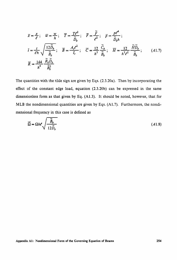
D,h

_ 12D, -~ A — CG - ine | —>. B= _ ca, H=

th B, r h B,

_ R,D R= 144 Reds B,

The quantities with the tilde sign are given by Eqs. (2.3.20a). Then by incorporating the

effect of the constant edge load, equation (2.3.20b) can be expressed in the same

dimensionless form as that given by Eq. (A1.3). It should be noted, however, that for

MLB the nondimensional quantities are given by Eqs. (A1.7). Furthermore, the nondi-

mensional frequency in this case is defined as

Appendix Al: Nondimensional Form of the Governing Equation of Beams

(A1.8)

254

Appendix A2: Determining the Positiveness of an

Expression

Denote the expression inside the square root sign of Eq. (3.2.7a) as

0, = 07 — 4(1 + TF) RQ — BQ’)

where

Substituting Eq. (A2.2) into Eq. (A2.1), one obtains

O,={(C + HT) — 41+ TF)R}Q’

+ {411 + TF)B —2(C + HT)T}Q° + T°

First, consider the case with T=0. As a result, equation (A2.3) is reduced to

O, = (C* — 4R)Q + 40?

Appendix A2: Determining the Positiveness of an Expression

(A2.1)

(A2.2)

(A2.3)

(A2.4)

255

From Eq. (A2.4), it can be seen that C?— 4R >0 is a sufficient condition for Q, to be

positive. One can check whether this condition is satisfied. From Appendix Al, for SLB

one has

= 6)E B’ E c-$) E- Fhe

5 . 6(l1—p) E' (A2.5)

— 6

R=-5 G'

Therefore,

=? ype, 36 E12 OE 1h EY CAR =r las G5 Ton BTU - SIF?

(A2.6) >£(36£ 12 12 £)

G' ‘25 G' 5 25 l—u E

Denote

> 36 E£ 12 12 4 E Os=95°G "5-25 I-n E (42.7)

It can be seen from Eq. (A2.6) that Q, > 0 is a sufficient condition for C?— 4R > 0 which

in turn is the condition to ensure Q,> 0 for the case with T= 0.

The condition Q, > 0 can be written as

, Ub

l-—yp

E35 ,1 E Gi > 3 + 3 E (A2.8)

It is evident that Eq. (A2.8) is satisfied for a wide range of practical composite material

properties.

One can specialize Eq. (A2.6) for the case of isotropic materials (i.e.,

E=F,G=G',p' =pand G=E/2(1+p)). It yields

Appendix A2: Determining the Positiveness of an Expression 256

C? — aR = 1 — (49 + 36 — 132u? — 96? + 144y*) (A2.9) 25(1 — 2)

It is known that for isotropic materials, the Poisson ratio » can only have values between

—1and0.5. Denote

Os = 49 + 36u — 1132p? — 96p? + 1144p" (A2.10)

Then for —1<y<0.5, it can be verified that Q,>0. Hence, if T= 0, for isotropic ma-

terials the condition C? — 4R > 0 is always satisfied.

Next, consider Eq. (A2.3) and denote ( T #0)

0O,=(C+HT) —-4(1+TF)R ee A211

=(C?—4R)+(2CH —4FR)T + H’°T° (

O, =4(1+ TF)B —2C+HT)T St A2.12

= 4B + (4BF —2C)T -2HT” ae)

As can be seen from Eq. (A2.3), Q,;>0and Q,>0 give a sufficient condition for

Q,>0. One can examine whether these relations are satisfied. First, equation (A2.11)

is considered. The coefficient of T in this equation, according to Appendix Al, can be

expressed as

cH —aFR 124 £ HE 6 E 2CH —4FR= Bap G {seu l—-n E 6 G (A2.13) 5

From Eq. (A2.13), one observes that

2CH —4FR <0 (A2.14)


is valid for large E/G’ values. However, it should be noted that the dimensionless

quantity T is a very small quantity according to its definition which is

IT) =| Fe << (A2.15) EI

This is true if

ITIeW<<El (A2.16)

The symbol | | denotes the absolute value of the quantity inside the vertical bars. It

can be seen, furthermore, from Eqs. (A2.6) and (A2.13) that one has

~ — A? — o_ [C’ — 4R] ~[—— (2CH — 4FR)) (A2.17)

Pr

for large E/G’ values, where the symbol ~ means the orders of magnitude of the quan-

tities on both sides are the same.

Consider beams with rectangular cross sections (having the width 5 and the depth

h). Hence, one has

—— =174/ (A2.18)

If, for example, ?/h = 10, in view of Eq. (A2.18), one can also express Eq. (A2.17) as

follows:

[C* —4R] ~ [2CH — 4FR]x 10° (A2.19)

In view of Eqs. (A2.16) and (A2.19), one finds that the relation

C*—4R >> |(2CH — 4FR)T| (A2.20)


should hold true in general. As a result, Q, is greater than zero.

Next, examine Eq. (A2.12). First, the coefficient of T in this equation is considered.

It can be expressed as

4BF —-2C =—+ = - + —_ + -2 (A2.21)

which is greater than zero if

, _# 6 l—u Food _E a >t = (A2.22)

Equation (A2.22) will be valid for a wide range of practical composite material proper-

ties since generally the value of E/G’ is quite large (for example, from 20 to 50). Fur-

thermore, comparing the orders of magnitude of terms in Eq. (A2.12), one finds that

2

— Ag ok 4B = 4—— > > | (4BF — 2C)T| (A2.23a)

4B >> |2HT"| (A2.236)

In view of Eqs. (A2.22) and (A2.23), generally one can regard Q, to be greater than zero.

From the above discussion, one concludes that for single-layered transversely

isotropic beams, practically Q, can be considered to be positive.


Appendix A3: Derivation of Modal Equations

The governing equation for bending motion of linear elastic structural members,

when the rotatory inertia is neglected but including the transverse shear deformation

effects, can be expressed in the following form (for simplicity, a one-dimensional struc-

tural member is assumed):

2

LCw(x,t)] + Col £ w(x,)] + My = w(x,0] = FLp(x,)] ont (A3.1a)

The boundary conditions are assumed to be homogeneous and denoted by

Bw(x,)]=0 on dt (A3.1)

where

L, the linear spatial differential operator associated with the elastic prop-

erty (stiffness) of the structure,

C, the linear spatial differential operator associated with the damping ef-

fect acting on the structure,

Appendix A3: Derivation of Modal Equations 260

M, the linear spatial differential operator associated with the inertia effect

of the distributed mass of the structure,

F, the linear spatial differential operator associated with the external

transverse load intensity, p(x,2),

w(x,t) the transverse displacement,

B, the linear spatial differential operator associated with the boundary

conditions,

t, OT the domain and boundary of the structure.

The essence of the modal analysis is to employ the orthogonal (biorthogonal)

properties of the eigenfunctions belonging to the self-adjoint (non-self-adjoint) system

[84,85] to decouple governing equations described by linear partial differential equations

into an infinite number of independent modal equations. Each modal equation is de-

scribed by a linear ordinary differential equation which can be solved much easily. The

aim, hence, is to find the general solution of the governing equations, which can be ex-

pressed in terms of the solutions of the modal equations.

The material described herein follows closely that in [84]. Assume that L, and M,

are both self-adjoint and positive definite (for the non-self-adjoint case, see [85]). First,

the free vibration problem is considered. The eigenvalue problem of undamped struc-

tures is (let w(x,0) = w(x)e™ )

L,[w]='M,[w] on +t (A3.2a)

with the boundary condition

Bw]=90 on dt (A3.26)


Assume that the eigenvalue problem is solved, and infinite denumerable sets of

eigenvalues and eigenfunctions, (Q?, w,(x)) , are available. In view of Eq. (A3.2a), for

any two distinct pairs of eigenvalues and eigenfunctions, (2, w,) and (2, w,) , one has

L,Lw,] = Q7M,[w,] (A3.3a)

L,[w,] = Q3M,Cw,] (A336)

Define

(u, Lov) = | uL,[vjdt (A3.4a)

(u, M,v) = | uM [v]dt (A3.4b)

where u and v are two arbitrary eigenfunctions. According to Eqs. (A3.3), one can form

an integral as

| owetptw _ w,L,[ws;])az = [ o2w.M,tw3 _ Ofw,M,Lw,])dt (A3.5)

In view of the definitions given by Eqs. (A3.4) and taking into account the self-adjont

property of the operators L, and , , ie.,

(u, Lov) = (v, Lpu) (A3.6a)

and


(u, M,v) = (v, M,u) (43.66)

where u and v are two arbitrary eigenfunctions, from Eq. (A3.5) one obtains

0 = (Q; ~ Q5)(W,, Mpw,) (A3.7)

Since it was assumed that Q,#Q, , according to Eq. (A3.7), the following orthogonal

relation is found:

(w,, Mw, =0, r#s (A3.8)

Furthermore, from Eqs. (A3.3a) and (A3.8), one obtains another orthogonal relation

(w,, L,w,))=0, r#s (A3.9)

However, when r=s, the value of (w,, \f,w,) is no longer zero. It is a positive number

(which is also referred to as the norm) for M, is positive definite. When the

eigenfunctions are normalized as

(w,, Mw, =1, r=1,2,... (A3.10)

then, in view of Eqs. (A3.3a) and (A3.10), one has

(W,, L,W,) = 22, r=1,2,... (A3.11) P

In terms of the normalized eigenfunctions defined by Eq. (A3.10), the orthogonal re-

lations, 1.e., Eqs. (A3.8) and (A3.9), together with Eqs. (A3.10) and (A3.11) can be

written in more compact form as

(W,, MpW,) = 5p (A3.12a)


(W,, LpW,) = 276, (A3.125)

where 6,, is the Kronecker symbol.

Next, one can derive the modal equations using the obtained eigensolutions and

orthogonal relations. According to the expansion theorem [84,85], the solution, w(x, 2),

can be expressed in the following form:

w(x, = > Wxa() (43.13) i=1

where w(x) are the normal modes defined by Eq. (A3.10) and q(t) are time-dependent

generalized coordinates.

Introducing Eq. (A3.13) into Eq. (A3.1a) and applying the Galerkin procedure [96],

in view of Eqs. (A3.12), one obtains

Gl) + Dorie) + Qa =L(, r= 1,2, (43.14a) i=l

where

Cy = (W,, CpW)) (43.146)

are damping coefficients and

S(t) = (Wp Fy p(x, 0) (A3.14c)


are generalized forces. Equations (A3.14a) represent an infinite set of coupled ordinary

differential equations where the coupling comes from the damping terms. However, in

a special case when

C,= aL, + aM, (A3.15)

where a, and a, are real constants, Equations (A3.14a) become decoupled. This can be

seen as follows:

A A

C1 = (W,, C,W))

A

=(w,, (aL, + a,M,) Ww)

A A

= ay (W,, L,w)) + a,(W,, M,w,)

= (4,2; + @)5,

Denoting the modal damping ratio of the rth mode as

b= (a,Q,? + a) r 20,

one can then express Eqs. (A3.14a) as follows:

G(t) + 2E,2.4(t) + Q¢(N=f(t), r=1,2,...

(A3.16)

(A3.17)

(A3.18)

These are the modal equations obtained under the assumption that the operator C, sat-

isfies the relation described by Eq. (A3.15).


Appendix A4: Dimensionless Form of the Governing

Equation of Plates

The case of single-layered transversely isotropic plates (SLP) and of multilayered

transversely isotropic plates (MLP) are considered separately in the following. For

4

convenience, the changes of notation, x, ~ x and x, > y, are made.

4

Single-layered Transversely Isotropic Plates

If the plate is assumed to be subjected to constant in-plane edge loads T, and 7,

(which are applied in the directions parallel to the x and y axes, respectively, and are

considered positive in tension), the governing equation given by Eq. (2.3.22a) must be

slightly modified by making the substitution, P3 > Pp; + T,w,,+ T,w,,. To convert the

resulting governing equation into a nondimensional form, the following dimensionless

quantities as defined are used:

eakX. get. cit. FES 1 “2p x f,' y=’ veh? R67? G’’

(2 fy. ed B=12 h (F y; DF ’ 2D,’

Appendix A4: Dimensionless Form of the Governing Equation of Plates 266

, _ é _

£5," £yi5). G=(yG;

AMEE ma G8 @i-w E (F, T, = T.

7, = 1201 — ey LAF pot, Rewa-Ayo i

Rares Hoy air (44.1)

U7 l - E H =———— ; fat /—4—, ora ail “1 V o(l—H)

P3 2 ce) 2 ! = 120 = 2) (yh

Making use of Eqs. (A4.1), one obtains the governing equation for the transverse vi-

bration of SLP in dimensionless form as

_ gt 2 6,R22 4 52H (645,87) Ce 7a ~(€, +6,HT,) Ge .

or’ ax*ér? yor

~ (F224 F244 FF) LE 4 BF oy 8 4.2 1 ar 2 ay 1 Fy ax’ 142 24 axay (A4.2)

Ho Pp ap 5 +(D, + TE =p-(F, +7, 2) 46,7 2 2 2) ay P ( ax? 2 ay 7) A ar

For the free vibration problem, the nondimensional frequency is defined as

2

Q= ar, Ee? (A4.3)

Multilayered Transversely Isotropic Plates

Similar to the case of SLP, the following nondimensional quantities are introduced:

Appendix Ad: Dimensionless Form of the Governing Equation of Plates 267

y= eo J. tL Ww _ 2,2 RD x= ¢, 9 J t, 9 Ww h , R 144( t} ) h* RB? ’

¢, 2 9 2 \2 C = 1 2 B= (ey Ga e Yes Gals

72 bt 7 TG. 5 “as = ~ 17 ~ oY 27 ~ 3 . (ih? B D D (44.4)

~ 4%. = J =~ F. <s_ F =|"); D ==; =—7,; ="-7; 1 (7, ) 2 D, 1 2 2 2

{ee Dp = B p= iz) py, t= c 12D ; B=0¢,) Be

Dh 1 B 12D

The quantities with the tilde sign are defined as follows:

~ MoM, ~ * ~

R= ——; B=M; D=D*,; S

~ : B F L’ .

C= Mol + 69( > - 1 + 54M; A4.5 SF MS “ (44)

~ * * ~ vf.

Fo4--5,4; A= S S S

while all the quantities with the star sign are given by Eqs. (2.3.17c).

Making use of the definitions given by Eqs. (A4.4), one can convert the governing

equation for the transverse vibration of MLP into the same dimensionless equation as

Eq. (A4.2).

Appendix A4: Dimensionless Form of the Governing Equation of Plates 268

Appendix B1: The Integral Solution Form of Linear

Systems

Consider the linear system which is expressed in state-variable form as follows:

x(t) = Ax(2) + f(a) (B1.1)

where the system matrix A is assumed constant. The solution of Eq. (B1.1) can be ex-

pressed in integral form for an arbitrary initial condition x(¢,) as [91]

X(t) = V(t — f)x(fo) + | ‘Y(t — a)f(x) de (B1.2) 4

where ‘Y(t — t) is the transition matrix. Two of the important properties of the transition

matrix are

F(t) — &) = F(q — B)Y(Q — 43) (B1.3)

Y(t — b) = ¥(Q - 4) (B1.4)

Appendix Bi: The Integral Solution Form of Linear Systems 269

To obtain the solution of Eq. (B1.1) in an integral form for given terminal states of the

process, x(t), one proceeds as follows:

First, let ¢ = ¢, in Eq. (B1.2), which results in

X(t) = ‘¥ (tp — f9)X(fo) + | "vy t)f(r) dr (B1.5)

Solving for x(t) from Eq. (B1.5) and substituting it into Eq. (B1.2), one obtains

x(t) = V(t— yey ofa _ | Wy- t)f(z) é|h f ; (B1.6)

+ | Y(t — t)f(z) at %

According to Eqs. (B1.3) and (B1.4), one has

V(t = to) ¥' (ty ~ tg) = ¥(t — bo) M(o — ) = ¥(E- 9) (B1.7)

Y(t — t)'¥(tp— t) = ‘P(t — 1) (B1.8)

Note also that for 4, < ¢ < t, (assume that the integrand is a continuous function of time)

| "wor — a)f(c) de = | ‘W(r— afl) de + | "V(r — tft) de (B19) lo ly t

Then, making use of Eqs. (B1.7), (B1.8) and (B1.9), one obtains from Eq. (B1.6)

Appendix B1: The Integral Solution Form of Linear Systems 270

x(t) = F(t — t)x(f) — [ve — t)f(r) dt

st (B1.10) = ¥(t— t)x(t) + | Y(t — t)f(t) dt

y

This final equation is used for Eq. (4.2.16).

Appendix B1: The Integral Solution Form of Linear Systems 271

REFERENCES

1. Meirovitch, L. and Baruh, H., “Control of Self-Adjoint Distributed-Parameter Sys-

tems,” Journal of Guidance, Control, and Dynamics, Vol. 5, No. 1, 1982, pp. 60-66.

2. Meirovitch, L., Baruh, H. and Oz, H., “Comparison of Control Technique for Large

Flexible Systems,” Journal of Guidance, Control, and Dynamics, Vol. 6, No. 4, 1983,

pp. 302-310.

3. Bennighof, J. K. and Meirovitch, L., “Active Vibration Control of a Distributed

System with Moving Support,” Journal of Vibration, Acoustics, Stress, and Reliability

in Design, Vol. 110, April 1988, pp. 246-253.

4. Balas, M. J., “Active Control of Flexible Systems,” Journal of Optimization Theory

and Applications, Vol. 25, No. 3, 1978, pp. 415-436.

5. Skidmore, G. R. and Hallauer, W. L., “Modal-Space Active Damping of a Beam-

Cable Structure: Theory and Experiment,” Journal of Sound and Vibration, Vol. 102,

No. 2, 1985, pp. 149-160.

6. Hallauer, W. L., Skidmore, G. R. and Gehling, R. N., “Modal-Space Active

Damping of a Plane Grid: Experiment and Theory,” Journal of Guidance, Control,

and Dynamics, Vol. 8, No. 3, 1985, pp. 366-373.

REFERENCES 272

10.

11.

12.

13.

14.

15.

Aubrun, J. N., Ratner, M. J. and Lyons, M. G., “Structural Control for a Circular

Plate,” Journal of Guidance, Control, and Dynamics, Vol. 7, No. 5, 1984, pp. 535-545.

Ulsoy, A. G., “Vibration Control in Rotating or Translating Elastic Systems,”

Journal of Dynamical Systems, Measurement, and Control, Vol. 106, March 1984, pp.

6-14.

Biswas, S. K., and Ahmed, N. U., “Stabilization of a Class of Hybrid Systems Aris-

ing in Flexible Spacecraft,” Journal of Optimization Theory and Applications, Vol. 50,

No. 1, 1986, pp. 83-108.

Fukuda, T., Arai, F., Hosogai, H. and Yajima, N., “Flexibility Control of Flexible

Structures (Modeling and Control Method of Bending-Torsion Coupled

Vibration),” JSME International Journal, Series III, Vol. 31, No. 3, 1988, pp.

575-582.

Murotsu, Y., Okubo, H., Matsumoto, H., Okawa, Y. and Terui, F., “Tendon Con-

trol System for Flexible Space Structures,” Bulletin of University of Osaka Prefecture,

Series A, Vol. 34, No. 1, 1985, pp 1-11.

Murotsu, Y., Okubo, H., Mitsuya, A. and Terui, F., “Tendon Control of Flexible

Structure - A Hardware Demonstration,” Bulletin of University of Osaka Prefecture,

Series A, Vol. 35, No. 2, 1986, pp. 101-109.

Meirovitch, L., Baruh, H., Montgomery, R. C. and William, J. P., “Nonlinear Na-

tural Control of Experimental Beams,” Journal of Guidance, Control, and Dynamics,

Vol. 7, No. 4, 1984, pp. 437-442.

Schaechter, D. B., “Hardware Demonstration of Flexible Beam Control,” Journal

of Guidance, Control, and Dynamics, Vol. 5, No. 1, 1982, pp. 48-53.

Schaechter, D. B. and Eldred, D. B., “Experimental Demonstration of the Control

of Flexible Structures,” Journal of Guidance, Control, and Dynamics, Vol. 7, No. 5,

1984, pp. 527-534.

REFERENCES 273

16.

17.

18.

19.

20.

21.

22.

23.

24.

25.

Schafer, B. E. and Holzach, H., “Experimental Research on Flexible Beam Modal

Control,” Journal of Guidance, Control, and Dynamics, Vol. 8, No. 5, 1985, pp.

597-604.

Walker, L. A. and Yaneske, P. P., “Characteristics of an Active Feedback System

for the Control of Plate Vibration,” Journal of Sound and Vibration, Vol. 46, No. 2,

1976, pp. 152-176.

Walker, L. A. and Yaneske, P. P., “The Damping of Plate Vibrations by Means of

Multiple Active Control Systems,” Journal of Sound and Vibration, Vol. 46, No. 2,

1976, pp. 177-193.

Chung, L. L., Reinhorn, A. M. and Soong, T. T., “Experiments on Active Control

of Seismic Structures,” Journal of Engineering Mechanics, Vol. 114, No. 2, Feb. 1988,

pp. 241-256.

Baz, A., Gilheany, J. and Steimel, P., “Active Vibration Control of Propeller

Shafts,” Journal of Sound and Vibration, Vol. 136, No. 3, 1990, pp. 361-372.

Firoozian, R. and Stanway, R., “Modelling and Control of Turbomachinery Vi-

brations,” Journal of Vibration, Acoustics, Stress, and Reliability in Design, Vol. 110,

Oct. 1988, pp. 521-527.

O’Donoghue, P. E. and Atluri, S. N., “Control of Dynamic Response of Continuum

Model of a Large Space Structure,” Computers & Structures, Vol. 23, No. 2, 1986,

pp. 199-209.

Wang, P. K. C., “Feedback Control of Vibrations in an Extendible Wing,” Dynamics

and Stability of Systems, Vol. 3, Nos. 3 & 4, 1988, pp. 109-133.

Meirovitch, L. Dynamics and Control of Structures, Wiley-Interscience, 1990.

Leipholz, H. H. E. and Abdel-Rohman, M., Control of Structures, Martinus Nijhoff

Publishers, 1986.

REFERENCES 274

N

_

‘ ~

26.

27.

28.

29.

30.

31.

32.

33.

34.

35.

36.

Nurre, G. S., Ryan, R. S., Scofield, H. N. and Sims J. L., “Dynamics and Control

of Large Space Structures,” Journal of Guidance, Control, and Dynamics, Vol. 7, No.

3, Sept.-Oct. 1984, pp. 514-526.

Yang, J. N. and Soong T. T., “Recent Advances in Active Control of Civil Engi-

neering Structures,” Probabilistic Engineering Mechanics, Vol. 3, No. 4, 1988, pp.

179-188.

Nashif, A. D., Jones, D. I. G. and Henderson, J. P., Vibration Damping, John Wiley

& Sons Inc., 1985.

Horikawa, H., Dowell, E. H. and Moon, F. C., “Active Feedback Control of a Beam

Subjected to a Nonconservative Force,” International Journal of Solid and Struc-

tures, Vol. 14, pp. 821-839.

Takahashi, M. and Slater, G. L., “Design of a Flutter Mode Controller Using Posi-

tive Real Feedback,” Journal of Guidance, Control, and Dynamics, Vol. 9, No. 3,

May-June 1986, pp. 339-345.

Fuller, C. R., “Active Control of Sound Transmission/Radiation from Elastic Plates

by Vibration Inputs: I. Analysis” Journal of Sound and Vibration, Vol. 136, No. 1,

1990, pp. 1-15.

Jones, R. M., Mechanics of Composite Materials, Hemisphere Publishing Co., New

York, 1975.

Vinson, J. R. and Chou, T. W., Composite Materials and Their Use in Structures,

Applied Science Publishers Ltd., London, 1975.

Ambartsumian, S. A., Theory of Anisotropic Plates, Technomic Publishing Co., 1970.

Librescu, L., Elastostatics and Kinetics of Anisotropic and Heterogeneous Shell - Type

Structures, Sijthoff & Noordhoff, The Netherlands, 1975.

Whitney, J. M., Structural Analysis of Laminated Anisotropic Plates, Technomic

Publishing Co., 1987.

REFERENCES 275

37.

38.

39,

40.

41.

42.

43.

44,

45.

Reddy, J. N., “On the Solutions to Forced Motions of Rectangular Composite

Plates,” Journal of Applied Mechanics, Vol. 49, June 1982, pp. 403-408.

Reddy, J. N. and Phan, N D.,“Stability and Vibration of Isotropic, Orthotropic and

Laminated Plates According to a Higher-Order Shear Deformation Theory,” Journal

of Sound and Vibration, Vol. 98, No. 2, 1985, pp. 157-170.

Sciuva, M. D., “Bending, Vibration and Buckling of Simply Supported Thick

Multilayered Orthotropic Plates: An Evaluation of a New Displacement Model,”

Journal of Sound and Vibration, Vol. 105, No. 3, 1986, pp. 425-442.

Craig, T. J. and Dawe, D. J., “Flexural Vibration of Symmetrically Laminated

Composite Rectangular Plates Including Transverse Shear Effect,” International

Journal of Solids and Structures, Vol. 22, No. 2, 1986, pp 155-169.

Whitney, J. M., “The Effect of Transverse Shear Deformation on the Bending of

Laminated Plates,” Journal of Composites, Vol. 3, July 1969, pp. 534-547.

Sun, C. T. and Whitney, J. M., “Dynamic Response of Laminated Composite Plates

Under Initial Stress,” AAA Journal, Vol. 14, No. 2, 1976, pp. 268-270.

Khdeir, A. A., Analytical Solutions for the Statics and Dynamics of Rectangular

Laminated Plates Using Shear Deformation Theory, Ph.D. Dissertation, 1986,

Virginia Polytechnic and State University.

Librescu, L., Khdeir, A. A. and Reddy, J. N., “A Comprehensive Analysis of the

State of Stress of Elastic Anisotropic Flat Plates Using Refined Theories,” Acta

Mechanica, Vol. 70, 1987, pp. 57-81.

Librescu, L. and Khdeir, A. A., “Analysis of Symmetric Cross-ply Laminated Elastic

Plates Using a Higher-order Theory: Part I - Stress and Displacement & Part II -

Buckling and Free Vibration,” Composite Structures, Vol. 9, 1988, pp. 189-213 &

259-277.

REFERENCES 276

46.

47.

48.

49.

50.

SI.

52.

33.

54.

55.

36.

Srinivas, S. and Rao, A. K., “Bending, Vibration and Buckling of Simply Supported

Thick Orthotropic Rectangular Plates and Laminates,” International Journal of Sol-

ids and Structures, Vol. 6, 1970, pp. 1463-1481.

Stein, M. and Jegley, D. C., “Effects of Transverse Shearing on Cylindrical Bending,

Vibration, and Buckling of Laminated Plates,” AJAA Journal, Vol. 25, No. 1, Jan.

1987, pp. 123-129.

Gordaninejad F. and Ghazavi, A., “Effect of Shear Deformation on Bending of

Laminated Composite Beams,” Journal of Pressure Vessel Technology, Vol. 111,

May 1989, pp. 159-164.

Timishenko, S. P. and Woinowsky-Krieger, S., Theory of Plates and Shells, 2nd

Edition, McGraw Hill, New york, 1959.

Reissner, E., “The Effect of Transverse Shear Deformation on the Bending of Elastic

Plates,” Journal of Applied Mechanics, Vol. 12, June 1945, A69 - A77.

Mindlin, R. D., “Influence of Rotatory Inertia and Shear on Flexural Motion of

Isotropic Plates,” Journal of Applied Mechanics, Vol. 18, March 1951, pp. 31-38.

Timoshenko, S. P., “On the Correction for Shear of the Differential Equation for

Transverse Vibration of Prismatic Bars,” Philosophical Magazine, Series 6, Vol. 41,

1921, pp. 744-746.

Cowper, G. R., “The Shear Coefficient in Timoshenko’s Beam Theory,” Journal of

Applied Mechanics, Vol. 33, June 1966, pp. 335-340.

Bank, L. C., “Shear Coefficients for Thin-Walled Composite Beams,” Composite

Structures, Vol. 8, 1987, pp. 47-61.

Librescu, L., “On the Theory of Anisotropic Elastic Shells and Plates,” [nternational

Journal of Solids and Structures, Vol. 3, 1967, pp. 53-68.

Librescu, L. and Reddy, J. N., “A Critical Review and Generalization of Transverse

Shear Deformable Anisotropic Plates Theories,” Euromech Colloquium 219, Refined

REFERENCES 277

57,

38.

59.

60.

61.

62.

63.

65.

Dynamical Theories of Beams, Plates, and Shells and Their Applications, Kassel, Sept.

23-26, 1986.

Reissner, E., “Reflections on the Theory of Elastic Plates,” Applied Mechanics Re-

views, Vol. 38, No. 11, Nov. 1985, pp. 1453-1464.

Green, A. E. and Naghdi, P. M., “A Theory of Laminated Composite Plates,” JMA

Journal of Applied Mathematics, Vol. 29, 1982, pp. 1-23.

Librescu, L. and Reddy, J. N., “A Few Remarks Concerning Several Refined Theo-

ries of Anistropic Composite Laminated Plates,” International Journal of Engineer-

ing Science, Vol. 27, No. 5, 1989, pp. 515-527.

Reddy, J. N., “A Simple High-Order Theory for Laminated Composite Plates,”

Journal of Applied Mechanics, Vol. 51, December 1984, pp. 745-752.

Lo, K. H., Christensen, R. M. and Wu, E. M., “A High-Order Theory of Plate De-

formation, Part 1: Homogeneous Plates & Part 2: Laminated Plates,” Journal of

Applied Mechanics, Vol. 44, December 1977, pp. 663-668 & 669-676.

Toledano, A. and Murakami, H., “A High-Order Laminated Plate Theory with Im-

proved In-Plane Responses,” International Journal of Solids and Structures, Vol. 23,

No. 1, 1987, pp. 111-131.

Chen, P. S. and Archer R. R., “Solution of a Twelfth Order Thick Plate Theory,”

Acta Mechanica, Vol. 79, 1989, pp 97-111.

. Adali, S., Sadek, I. S., Sloss, J. M. and Bruch, J. C., “Distributed Control of Layered

Orthotropic Plates with Damping,” Optimal Control Applications & Methods, Vol.

9, 1988, pp. 1-17.

Sadigh-Esfandian, R., Sloss, J. M. and Bruch, J. C., “Optimal Control of a Pre-

stressed, Orthotropic Thin Cylindrical Shell Subjected to a Constant Pressure at its

Interior Wall,” Journal of Sound and Vibration, Vol. 125, No. 1, 1988, pp. 123-130.

REFERENCES 278

66.

67.

68.

69.

70.

71.

72.

73.

74,

75.

76.

Sadek, I. S., Sloss, J. M., Bruch, J. C., Jr., and Adali, S., “Optimal Control of a

Timoshenko Beam by Distributed Forces,” Journal of Optimization Theory and Ap-

plications, Vol. 50, No. 3, September 1986, pp. 451-461.

Sadek, 1. S., Sloss, J. M., Bruch, J. C., Jr., and Adali, S., “Structural Control to

Minimize the Dynamic Response of Mindlin-Timoshenko Plates,” Journal of the

Franklin Institute, Vol. 324, No. 1, 1987, pp. 97-111.

Kim, J. U. and Renardy, Y., “Boundary Control of the Timoshenko Beam,” SIAM

Journal of Control and Optimization, Vol. 25, No. 6, November 1987, pp. 1417-1429.

Garber, A. M., “Pyrolitic Materials for Thermal Protection Systems,” Aerospace

Engineering, Jan. 1963, pp. 126-137.

Wu, C. I. and Vinson, J. R., “Free Vibrations of Plates and Beams of Pyrolitic

Graphite Type Materials,” AIJAA Journal, Vol. 8, February 1970, pp. 246-251.

Daugherty, R. L., Kliger, H. S. and Vinson, J. R., “Governing Equations for Shells

of Pyrolitic Graphite Type Materials,” AJAA Journal, Vol. 9, No. 3, March 1971,

pp. 508-510.

Zukas, J. A. and Vinson, J. R., “Laminated Transversely Isotropic Cylindrical

Shells,” Journal of Applied Mechanics, Vol. 38, June 1971, pp. 400-407.

Wu, C. I. and Vinson, J. R., “Influences of Large Amplitudes, Transverse Shear

Deformation, Rotatory Inertia on Lateral Vibrations of Transversely Isotropic

Plates,” Journal of Applied Mechanics, Vol. 36, 1969, pp. 254-260.

Brunelle, E. J., “The Statics and Dynamics of a Transversely Isotropic Timoshenko

Beams,” Journal of Composite Materials, Vol. 4, July 1970, pp. 404-416.

Brunelle, E. J., “Elastic Instability of Transversely Isotropic Timoshenko Beams,”

AIAA Journal, Vol. 8, No. 12, December 1970, pp. 2271-2273.

Brunelle, E. J., “Buckling of Transversely Isotropic Mindlin Plates,” AJAA Journal,

Vol. 9, No. 6, June 1971, pp. 1018-1022.

REFERENCES 279

77,

78.

79.

80.

St.

82.

83.

84.

85.

86.

87.

Brunelle, E. J., “Stability and Vibration of Transversely Isotropic Beams Under In-

itial Stress,” Journal of Applied Mechanics, September 1972, pp. 819-821.

Brunelle, E. J., “Statics of Transversely Isotropic Beams,” AJAA Journal, Vol. 10,

No. 8, August 1972, pp. 1083-1085.

Chen, L. W. and Doong, J. L., “Vibrations of an Initially Stressed Transversely

Isotropic Circular Thick Plate,” [nternational Journal of Mechanical Science, Vol. 26,

No. 4, 1984, pp. 253-263.

Noor, A. K. and Burton, W. S., “Assessment of Shear Deformation Theories,” Ap-

plied Mechanics Reviews, Vol. 42, No. 1, Jan. 1989, pp. 1-11.

Librescu, L. and Stein, M.,“A Geometrically Nonlinear Theory of Shear Deformable

Laminated Composite Plates and Its Use in the Postbuckling Analysis,” JICAS Pro-

ceedings, 1\CAS-88-5.2.4., Jerusaleum, Israel, Aug. 28 - Sept. 2, 1988.

Levinson, M., “A New Rectangular Beam Theory,” Journal of Sound and Vibration,

Vol. 74, No. 1, 1981, pp. 81-87.

Clough, R. W. and Penzien, J., Dynamics of Structures, McGraw-Hill, Inc., 1975.

Meirovitch, L., Analytical Methods in Vibrations, The Macmillan Co., New York,

1967.

Meirovitch, L., Computational Methods in Structural Dynamics, Sijthoff &

Noordhoff, The Netherlands, 1980.

Traill-Nash, R. W. and Collar, A. R., “The Effects of Shear Flexibility and Rotatory

Inertia on the Bending Vibration of Beams,” Quarterly Journal of Mechanics and

Applied Mathematics, Vol. 6, Part 2, 1953, pp. 186-222.

Huang, T. C., “The Effects of Rotatory Inertia and of Shear Deformation on the

Frequency and Normal Mode Equations of Uniform Beams with Simple End Con-

ditions,” Journal of Applied Mechanics, Vol. 28, December 1961, pp. 579-584.

REFERENCES 280

Vv,

88.

89.

90.

91.

92.

93.

94,

95.

96.

Crawley, E. F. and Luis, J. D., “Use of Piezoelectric Actuators on Elements of In-

telligent Structures,” AJAA Journal, Vol. 25, No. 10, 1987, pp. 1373-1385. Decem-

ber 1961, pp. 579-584.

Kirk, D. E., Optimal Control Theory, Prentice-Hall Inc., Englewood Cliffs, New

Jersey, 1970.

Kwakernaak, H. and Sivan, R., Linear Optimal Control Systems Wiley-Interscience,

New York, 1972.

Brogan W. L., Modern Control Theory, 2nd Edition, Prentice-Hall, Inc., 1985.

Kalman, R. E., “Contribution to the Theory of Optimal Control,” Sociedad

Mathematica Mexicana Boletin, 1960, pp. 102-119.

Potter, J. E., “Matrix Quadratic Solutions,” SIAM Journal on Applied Mathematics,

Vol. 14, No. 3, May 1966, pp. 496-501.

Arnold III, W. F. and Laub, A. J., “Generalized Eigenproblem Algorithms and

Software for Algebraic Riccati Equations,” Computer-Aided Control Systems Engi-

neering, Edited by M. Jamshidi and C. J. Herget, North-Holland, 1985.

Kim, Z. C., An Investigation of Methodology for the Control and Failure Identification

of Flexible Structures, Ph.D. Dissertation, 1986, Virginia Polytechnic and State

University.

Mikhlin, S. G., Variational Methods in Mathematical Physics, Translated by T.

Boddington, Pergamon Press, New York, 1964.

REFERENCES 281

VITA

The author was born on March 23, 1956 in Taiwan, R.O.C. He entered the Naval

Architecture and Marine Engineering Program at National Cheng Kung University at

Tinan, Taiwan in Aug. 1974, and received the B.S. degree in June 1978.

Upon graduation, he served two years of compulsory military service in the army.

After that he was employed as an assistant engineer by the United Ship Design and

Development Center at Taipei, Taiwan, from Aug. 1980 to Nov. 1982.

Then, he entered the M.S. program in Mechanical Engineering at State University

of New York at Buffalo in Jan. 1983, and obtained the M.S. degree in Aug. 1984. From

Feb. 1985 to Sept. 1985, he was employed as a mechanical design engineer by

Gulfstream Aerospace Corporation, Savannah, Georgia. He entered the Ph.D. program

in Engineering Mechanics at Virginia Polytechnic Institute and State University in Sept.

1985, and has studied toward the Ph.D. degree since then.

(Tw - “4 Chan |

Vita 282

active vibration control of composite structures - VTechWorks

Documents

Transcript of active vibration control of composite structures - VTechWorks