Active control of sound for improved music experience in vehicles
94
Michael Vanhoecke in vehicles Active control of sound for improved music experience Academiejaar 2012-2013 Faculteit Ingenieurswetenschappen en Architectuur Voorzitter: prof. dr. ir. Daniël De Zutter Vakgroep Informatietechnologie Master in de ingenieurswetenschappen: elektrotechniek Masterproef ingediend tot het behalen van de academische graad van Begeleiders: Mirjana Adnadevic, ir. Pieter Thomas Promotor: prof. dr. ir. Dick Botteldooren
-
Upload
khangminh22 -
Category
Documents
-
view
1 -
download
0
Transcript of Active control of sound for improved music experience in vehicles

Michael Vanhoecke
in vehiclesActive control of sound for improved music experience
Academiejaar 2012-2013Faculteit Ingenieurswetenschappen en ArchitectuurVoorzitter: prof. dr. ir. Daniël De ZutterVakgroep Informatietechnologie
Master in de ingenieurswetenschappen: elektrotechniekMasterproef ingediend tot het behalen van de academische graad van
Begeleiders: Mirjana Adnadevic, ir. Pieter ThomasPromotor: prof. dr. ir. Dick Botteldooren

Preface
Sound is a fascinating medium. During my stay at the Technical University of Denmark
in the first semester, I had the privilege of being introduced to their elaborate research
facilities, covering a broad range of sound-related applications. This master thesis was a
next step in employing my skills as an electronics engineer, to tackle a problem in the field
of audio.
My stay abroad also implied that this thesis had to be executed within a strict time
schedule. During the past 5 months all my time and energy was consumed by this project,
but the interesting topic resulted in a satisfied feeling at the end.
This work would not have been realized without the help of various people at Intec-
Acoustics whom I would like to thank.
Professor Botteldooren, for providing this interesting topic and the flexibility in my ap-
proach and schedule. Moreover, he could be counted on to tackle problems and to give
inspiration for new solutions.
Mima, for guiding me through my thesis and always keeping me motivated.
Pieter Thomas, for the help in building the amplifiers and proofreading my thesis.
Peter Guns, for the technical assistance in building the cabin and mounting the loudspeak-
ers.
Finally, I would like to express my appreciation to my family and friends surrounding me.
Special thanks to Fran for supporting me during all those evenings and weekends I was
working instead of doing more relaxing stuff together.
Michael Vanhoecke, 10/06/2013


Permissions
“De auteur geeft de toelating deze masterproef voor consultatie beschikbaar te stellen en
delen van de masterproef te kopieren voor persoonlijk gebruik.
Elk ander gebruik valt onder de beperkingen van het auteursrecht, in het bijzonder met
betrekking tot de verplichting de bron uitdrukkelijk te vermelden bij het aanhalen van
resultaten uit deze masterproef.”
“The author gives permission to make this master dissertation available for consultation
and to copy parts of this master dissertation for personal use.
In the case of any other use, the limitations of the copyright have to be respected, in
particular with regard to the obligation to explicitly state the source when quoting results
from this master dissertation”
Michael Vanhoecke, 10/06/2013


Active control of sound
for improved music experience in vehiclesby
Michael Vanhoecke
Master thesis submitted for obtaining the academic degree of
Master of Science in Electrical Engineering
Electronic Circuits and Systems
Academic year 2012-2013
Promotor: prof. dr. ir. D. Botteldooren
Supervisors: M. Adnadevic, Ir. P. Thomas
Faculty of Engineering and Architecture
Ghent University
Department of Information Technology - Acoustics
Head of Department: prof. dr. Ir. D. De Zutter
Summary
In this master thesis, the possibility of creating virtual 3D audio in a vehicle environmentis investigated. Based on the mechanisms of human sound source localization, binauralsignals can be used to present spatial information to the listener. For this, it is necessary tobe able to control the sound at the ears of a listener. However, when using loudspeakers,there is no passive channel separation present. Furthermore, multiple sound reflectionsin the cabin give rise to spectral deformation. To overcome this, an extended version ofthe crosstalk cancellation technique is introduced, to actively control the sound field atboth ears independently. Transfer functions from speakers to the ears are measured ina cabin and are used to design an inverse filter matrix. Different loudspeaker topologiesare tested to improve performance. A four channel system shows to have an improvedperformance over a basic two channel setup by including an additonal stereo dipole. Achannel separation higher than 20 dB is achieved in a frequency range of 200 Hz to 8 kHzat the optimal listening position while the rotational sweet spot is increased. ITD and ILDcues are tested to validate the quality of the 3D reproduction. The spatial information ispreserved for the optimal listening position using both setups. For a head rotation of 30°,the four channel system can also reproduce the correct ITD, but the increased sweet is notsufficient to reproduce the ILD.
Keywords
Virtual 3D audio, Crosstalk cancellation, Vehicle environment


Active control of sound for improved musicexperience in vehicles
Michael Vanhoecke
Supervisor(s): Mirjana Adnadevic, Pieter Thomas, Dick Botteldooren
Abstract— This article investigates the possibility of creating virtual 3Daudio in a vehicle environment. Based on the mechanisms of human soundsource localization, binaural signals can be used to present spatial infor-mation to the listener. However, when using loudspeakers, there is no pas-sive channel separation present. Furthermore, multiple sound reflectionsin the cabin give rise to spectral deformation. The crosstalk cancellationtechnique is implemented to actively control the sound field at both earsindependently. Transfer functions from speakers to the ears are measuredin a cabin and are used to design an inverse filter matrix. Different loud-speaker topologies are tested to improve the performance. A four channelsystem shows to have an improved performance over a basic two channelsetup by including an additonal stereo dipole. An improvement is notedin channel separation, sweet spot size, distortion and ability to reproducevirtual sources.
Keywords— Virtual 3D audio, Crosstalk cancellation, Vehicle environ-ment
I. INTRODUCTION
AUDIO in vehicles has always been a topic of interest. Al-most every car has its own sound system since listening to
music or the radio is the only type of entertainment that can becombined with driving a car. However, a vehicle is far from anideal listening environment. The audio spectrum is heavily in-fluenced by reflections on windows and resonances due to thesmall volume of the space. Moreover, speakers are often placedat non-conventional positions. [1]. An interesting approach toimprove the music experience is to create a virtual 3D audio en-vironment,making it possible to place sound sources anywherein space, without the need for a physical source to be present.Creating the exact sound field over a large area requires a lot ofloudspeakers and thus is impractical. Alternatively, the soundfield can be controlled only at the two ears of the listener to de-liver sound with spatial information. This method is referred toas binaural audio [2].
II. BINAURAL REPRODUCTION
Binaural signals can be obtained in two different ways. A firstway is to record them using an artificial head with microphonesat the places of the ear drums. A second way is to create a syn-thetic binaural signal by adding spatial information to a monosound. A key component in binaural audio is the Head-RelatedTransfer Function(HRTF). A set of HRTFs comprises the mainlocalization cues of the auditory system, being the interaurallevel and time differences and the monaural spectral deforma-tion introduced by the pinna. Convolving a mono signal witha set of HRTFs results in a pair of binaural signals, a processreferred to as binaural synthesis [2]. Binaural signals shouldbe delivered exactly at the ears, so they are suited to be usedwith headphones. However, headphones are not comfortable towear while driving a car. External loudspeakers can be used, butthis introduces the problem of crosstalk. Sound cannot be sent
to each ear independently anymore. The crosstalk cancellationtechnique is implemented to actively control the sound field atboth ears [2].
III. CROSSTALK CANCELLATION
A. Theory of Operation
A listening situation is characterized by a plant matrix H. Foran S channel loudspeaker setup, this is a 2×S matrix containingthe transfer functions from each of the speakers to both ears [3].The transfer functions include the speaker response, the head-related transfer function (HRTF) and the room influence. Theplant matrix describes the deformation of the sound before itreaches the ears. A filter matrix C is added before sound is sentto the speakers, to compensate for the plant matrix. A system inwhich the signals are delivered to the ears perfectly is describedby the unity matrix, so it is clear that the matrix C has to be theinverse of the plant matrix.
B. Inverse Filtering
It is generally very hard to calculate the exact inverse of theplant matrix. The response will be non-minimum phase becausesound is present in echoes resulting from room and pinna reflec-tions. Inverting a non-minimum phase response is only stablewhen being acausal, so a modelling delay has to be included[3]. Moreover, when deconvolving an impulse response, the op-timal filter is inevitable of infinite duration, which makes it notrealizable. The responses at the ears contain deep notches atcertain frequencies due to interference of reflections at the pin-nas and the room response. Hence, a perfect equalization wouldresult in a large amount of energy being sent to try to compen-sate for these notches. A method to calculate the inverse filtersis presented by Tokuno et al. [3] and combines least squaresinversion in the frequency domain and zeroth-order regulariza-tion. The solution for the crosstalk cancellation matrix is givenby
C = [HHH + βI]−1HH (1)
in which β is the regularization parameter. Regularization al-lows to control the effective duration of the filters and limit theenergy. It introduces a trade-off between performance and effortoptimization.
IV. VEHICLE SETUP
A cabin was built out of metal with a Plexiglas front windowand a roof made out of wooden panels in which the loudspeakersare mounted. Absorbent material is placed against the walls onthe inside of the cabin to create a realistic sound environment.

Fig. 1. Positions of the loudspeakers. The position of the head is marked with across
The positions of the loudspeakers are displayed in figure 1.The plant matrix is measured using a B&K HATS. The impulseresponses are truncated to 48000 samples to design the inversefilters. The transfer functions show a severe spectral deforma-tion. At low frequencies, peaks due to the resonances in thecabin are present, while at higher frequencies deep notches oc-cur, indicating destructive interference effects caused by roomand pinna reflections. There is no natural channel separation asa result of the the room influence. The system in the cabin isdesigned and tested for a limited frequency range of 80Hz to8000Hz.
V. RESULTS
In order to compare the efficiency of different setups, a linearsweep is sent to the left channel and different criteria are ex-tracted to quantify the performance. Ideally one would recoverthe sweep exactly at the left ear an record silence at the right ear.The channel separation gives the ratio of the sound level at theipsilateral ear to the level at the contralateral ear. The crosstalkfilters are designed for one specific position, so a movement ofthe head results in a reduced performance. The area in whichcrosstalk cancellation is achieved is called the sweet spot. Inthis work, only the rotational sweet spot is considered. Distor-tion is last property which is checked.A four channel system, comprising speakers 1,2,4,5, results inthe best performance. A channel separation over 20 dB wasachieved for the optimal listening position, which is a valuematching the (anechoic) performance of common systems [4].The two channel system with speakers 1 and 2 effectively can-cels crosstalk, but has a limited sweet spot for high frequencies.Speakers 4 and 5 are placed closely together and form a stereodipole [5]. They have a poor performance at low frequenciesbut result in a broad sweet spot for higher frequencies. Thefour channel systems manages to combine the assets of bothtwo channel systems. Results for the channel separation andfrequency response at the ears can be found in figures 2 and 3. Itcan be seen that there is almost no distortion, indicating that theinverse filtering also succeeds in equalizing the room response.The virtual 3D reproduction is tested by playing back binauralsignals through the crosstalk cancellation system and compar-ing the ITD and ILD of the recorded signals with those of theoriginal signals. At the optimal listening position, both the twochannel and four channel setup produce differences smaller thanthe human discrimination threshold. At a head rotation of 30 de-
grees, the cues are lost for the two channel setup, but the ITDis preserved with the four channel setup. Since the ITD cuedominates the ILD cue [2], the virtual source direction will bereproduced correctly for broadband sources.
102
103
−20
−10
0
10
20
30
40
Frequency (Hz)
Chan
nel
Sep
aration(dB)
0°10°20°30°
Fig. 2. Channel separation for different angles of head rotation calculated per1/3 octave band
102
103
−60
−40
−20
0
20
40
60
Frequency (Hz)
Mag
nitude(dB)
LeftRight
Fig. 3. Response at the two ears for a linear sweep throught the left channel
VI. CONCLUSION
A four channel crosstalk cancellation system was imple-mented in a vehicle environment, improving the performanceof a basic two channel setup. A channel separation over 20 dBwas achieved for the optimal listening position, matching com-mon systems [4]. Virtual source reproduction was correct for arotational sweet spot of 30 degrees, though only for broadbandsources. Subjective test should be performed to validate this.Further research consists of integrating the system in real-timeand possibly upgrading it to a dynamic system, which updatesthe inverse filters according to the position of the head.
REFERENCES
[1] A. Farina and E. Ugolotti, “Spatial equalization of sound systems in cars,”in Audio Engineering Society Conference: 15th International Conference:Audio, Acoustics and Small Spaces, 10 1998.
[2] W. Gardner, 3D Audio Using Loudspeakers. Springer, 1998.[3] H. Tokuno, O. Kirkeby,P. Nelson, and H. Hamada, “Inverse filter of sound
reproduction systems using regularization,” IEICE Transactions on Funda-mentals of Electronics, Communications and Computer Sciences, vol. 80,no. 5, pp. 809–820, 1997.
[4] B. Masiero, J. Fels, and M. Vorlander, “Review of the crosstalk cancellationfilter technique,” in International Conference on Spatial Audio, 2011.
[5] O. Kirkeby, P. Nelson, and H. Hamada, “Local sound field reproduction us-ing two closely spaced loudspeakers,” The Journal of the Acoustical Societyof America, vol. 104, no. 4, pp. 1973–1981, 1998.

Actieve geluidscontrole voor verbeterdemuziekervaring in voertuigen
Michael Vanhoecke
Supervisor(s): Mirjana Adnadevic, Pieter Thomas, Dick Botteldooren
Abstract—Dit artikel onderzoekt de mogelijkheid om virtuele 3D audiote creeren in een voertuigomgeving. Gebaseerd op de menselijke mechanis-men voor geluidslokalisatie, kunnen binaurale signalen gebruikt wordenom ruimtelijke informatie aan een luisteraar te presenteren. Wanneer erluidsprekers gebruikt worden, is er echter geen natuurlijke kanaalseparatieaanwezig. Bovendien resulteren reflecties in een ernstige spectrale vervor-ming. De crosstalk cancellation techniek wordt geımplementeerd om actiefhet geluid aan beide oren onafhankelijk te controleren. De transferfunctiesvan de luidsprekers tot de oren worden gemeten in een cabine and wordengebruikt om een inverse filter matrix te ontwerpen. Verschillende luidspre-keropstellingen worden getest om de performantie te verbeteren. Een vier-kanaals systeem vertoond een verbeterde performantie tegenover een basistweekanaals opstelling, door de toevoeging van een extra stereo dipool. Eris een verbetering in kanaalseparatie, sweet spot grootte, vervorming en demogelijkheid om virtuele bronnen te reproduceren.
Keywords—Virtuele 3D audio, Crosstalk cancellation, Voertuigomgeving
I. INTRODUCTIE
AUDIO in voertuigen is al sinds lang een onderwerp van in-teresse. Bijna elke auto heeft zijn eigen geluidssysteem,
aangezien naar muziek of de radio luisteren de enigste vorm vanontspanning is die kan gecombineerd worden met het besturenvan een auto. Een voertuig is echter verre van een ideale luis-teromgeving. Het audio spectrum wordt sterk beınvloed doorreflecties op ramen en resonanties door het kleine volume vande ruimte. Bovendien zijn luidsprekers vaak geplaatst op onge-wone posities [1]. Een interessante benadering om de muziek-ervaring te verbeteren is het creeren van een virtuele 3D audioomgeving, die toelaat om geluidsbronnen om het even waar teplaatsen zonder dat een physiche bron aanwezig moet zijn. Omhet geluidsveld exact te creeren over een groot gebied zijn eengroot aantal luidsprekers nodig, wat onpraktisch is. Een alter-natieve manier is om enkel het geluidsveld te controlleren aanbeide oren en geluid met ruimtelijke informatie af te leveren.Deze methode wordt binaurale audio genoemd [2].
II. BINAURALE REPRODUCTIE
Binaurale signalen kunnen verkregen worden op twee ver-schillende manieren. Een eerste manier is ze op te nemen meteen artificieel hoofd dat microfoons heeft op de plaats van detrommelvliezen. Een tweede manier is een synthetisch binau-raal signaal te creeren door ruimtelijke informatie toe te voegenaan een mono signaal. Een belangrijke component in binauraleaudio is de Head-Related Transfer Function(HRTF). Een setHRTFs bevat de belangrijkste lokalisatiemechanismen, zijndede interaural tijds- en niveauverschillen en de monaurale spec-trale vervorming door de oorschelp. De convolutie van eenmono signaal met een set HRTFs resulteerd in een paar binau-rale signalen, een techniek genaamd binaurale synthese [2].Binaurale signalen moeten exact aan de oren worden afgele-
verd en zijn dus geschikt om met een hoofdtelefoon te gebrui-ken. Hoofdtelefoons zijn echter niet comfortabel om te dra-gen tijden het besturen van een wagen. Externe luidsprekerskunnen worden gebruikt, maar dit introduceert het probleemvan crosstalk. Geluid kan nu niet meer onafhankelijk naar elkoor gestuurd worden. De crosstalk cancellation techniek wordtgeımplementeerd om het geluid aan beide oren actief te contro-leren [2].
III. CROSSTALK CANCELLATION
A. Werking
Een luistersituatie wordt gekarakteriseerd door een transfer-matrix H. Voor een S-kanaals luidspreker opstelling is dit een2 × S matrix die de transferfuncties van de luidsprekers tot deoren bevat [3]. The transferfuncties omvatten de response vande luidspreker, de HRTF en de invloed van de ruimte. De trans-fermatrix beschrijft de vervorming van het geluid voor het deoren bereikt. Een filter matrix C wordt toegevoegd voor dat hetgeluid naar de luidsprekers wordt gestuurd, om de transferma-trix te compenseren. Een systeem waarbij de signalen exact aande oren worden afgeleverd, wordt beschreven door de eenheids-matrix. Het is duidelijk dat de matrix C de inverse moet zijn vande transfermatrix.
B. Filterinversie
Het is doorgaans erg moeilijk om de exacte inverse van detransfermatrix te berekenen. De response zal niet-minimum-fase zijn, doordat er geluid aanwezig is in echo’s door reflectiesin de ruimte en op de oorschelpen. De inverse van een niet-minimum-fase respons is enkel stabiel wanneer ze acausaal is,bijgevolg moet een vertraging gemodelleerd worden [3]. Boven-dien zal bij de deconvolutie van een impulsantwoord, het opti-male filter van oneindige lengte zijn, waardoor het niet realiseer-baar is. De respons aan de oren bevat op bepaalde frequentiesscherpe pieken door de bijdragen van reflecties uit de ruimte ofop de oorschelp. Een perfecte egalisatie zou dus leiden tot eengrote hoeveelheid energie die nodig is die te compenseren. Eenmethode om de inverse filters te berekenen wordt voorgestelddoor Tokuno et al. [3] en combineert de kleinste-kwadraten in-versie met een regularisatie parameter. De oplossing voor decrosstalk cancellation matrix wordt gegeven door:
C = [HHH + βI]−1HH (1)
waarin β de regularisatieparameter is. Regularisatie laat toe omde effectieve lengte van de filters te reduceren en de energie telimiteren. Het introduceert een afweging tussen performantie enenergie optimalisatie.

IV. VOERTUIGOPSTELLING
Een cabine werd gebouwd uit metaal met een Plexiglas voor-uit en een dak gemaakt van houten panelen waarin de luidspre-kers worden gemonteerd. Absorberend materiaal wordt tegende wanden aan de binnenzijde geplaatst om een realistische ge-luidsomgeving te creeren. De posities van de luidsprekers wor-den getoond in figuur 1.
Fig. 1. Posities van de luidsprekers. De positie van het hoofd wordt aangeduidmet een kruis
De transfermatrix wordt opgemeten met een B&K HATS. Deimpulsantwoorden worden ingekort tot 48000 samples om deinverse filters te ontwerpen. De transfers functies vertonen eenernstige spectrale vervorming. Voor lage frequenties zijn pie-ker door de resonanties can de cabine te zien, terwijl scherpedalen aanwezig zijn voor hoge frequenties. Dit als gevolg vandestructieve interferentie, veroorzaakt door reflecties. Door deinvloed van de omgeving is er geen natuurlijke kanaaalseparatieaanwezig is. Het systeem in de cabine wordt getest voor eenfrequentiebereik van 80 8000Hz
V. RESULTATEN
Om de efficientie voor verschillende opstellingen te vergelij-ken, wordt een lineaire sweep door het linker kanaal gestuurden worden verschillende criterea afgeleid om de performantie tekwantificeren. Idealiter wordt de sweep exact gereproduceerdaan het linkeroor en is er stilte aan het rechteroor. De kanaalse-paratie geeft de verhouding van het geluidsniveau aan het ipsila-terale oor to het niveau aan het contralaterale oor. De crosstalkfilters worden ontworpen voor een specifieke positie, bijgevolgresulteert een beweging van het hoofd in een verminderde per-formantie. Het gebied waarin crosstalk cancellation wordt be-reikt wordt de sweet spot genoemd. Voor dit werk, wordt enkelde rotationele sweet spot in acht genomen. Vervorming is eenlaatste eigenschap die bekeken wordt.Een vierkanaals systeem, bestaande uit luidsprekers 1,2,4,5 le-vert de beste performantie. Een kanaalseparatie van meer dan20 dB werd bereikt voor de optimale luisterpositie. Dit is eenwaarde die overeenkomt met die van gebruikelijke (anechoi-sche) systemen. Het tweekanaals systeem met luidsprekers 1and 2 slaagt erin crosstalk effectief te onderdrukken, maar heefteen beperkte sweet spot voor hoge frequenties. Luidsprekers4 en 5 worden dicht bij elkaar geplaatst en vormen een stereodipool [5]. Ze hebben een slechte performantie voor lage fre-quenties, maar hebben een brede sweet spot voor hoge frequen-ties. Het vierkanaals systeem slaagt erin om de voordelen vanbeide tweekanaals systemen te combineren. Resultaten voor dekanaalseparatie en de frequentierespons aan de oren worden ge-
toond in figuren 2 en 3. Er is bijna geen distortie wat erop wijstdat de filterinversie er ook in slaagt de respons van de ruimte teegaliseren.De virtuele 3D reproductie wordt getest door binaurale signalenaf te spelen door het crosstalk cancellation systeem en de ITDen ILD van de opgenomen signalen te verglijken met die vande originele signalen. In de optimale luisterpositie resulterenzowel het tweekanaals als het vierkanaals systeem in verschil-len kleiner dan onderscheiden kunnen worden door de mens.Voor een hoofdrotatie van 30 graden gaan beide cues verlorenvoor het tweekanaals systeem, maar de ITD is bewaard voor hetvierkanaals systeem. Aangezien de ITD domineert over de ILD[2], zal de richting van de virtuele bron behouden blijven voorbreedbandige bronnen.
102
103
−20
−10
0
10
20
30
40
Frequency (Hz)
Channel
Sep
aration
(dB)
0°10°20°30°
Fig. 2. Kanaalseparatie voor verschillende hoofd rotaties berekend per tertsband
102
103
−60
−40
−20
0
20
40
60
Frequency (Hz)
Mag
nitude(dB)
LeftRight
Fig. 3. Respons aan de twee oren voor een lineare sweep door het linker kanaal
VI. CONCLUSIE
Een vierkanaals systeem werd geımplementeerd een voertui-gomgeving, met als resultaat een verbetering van de performan-tie tegenover een basis tweekanaals systeem. Een kanaalsepa-ratie van meer dan 20 dB werd bereikt voor de optimale luister-positie, gelijk aan gebruikelijke systemen [4]. De virtuele bronreproductie was correct voor een rotationele sweet spot tot 30graden, hoewel enkel voor breedbandige bronnen. Subjectievetests moeten worden uitgevoerd om dit te valideren. Verder on-derzoek bestaat uit het integreren van het systeem in real-timeen het mogelijks aanpassen tot een dynamisch systeem, dat deinverse filters aanpast naargelang de positie van het hoofd.

REFERENCES
[1] A. Farina and E. Ugolotti, “Spatial equalization of sound systems in cars,”in Audio Engineering Society Conference: 15th International Conference:Audio, Acoustics and Small Spaces, 10 1998.
[2] W. Gardner, 3D Audio Using Loudspeakers. Springer, 1998.[3] H. Tokuno, O. Kirkeby,P. Nelson, and H. Hamada, “Inverse filter of sound
reproduction systems using regularization,” IEICE Transactions on Funda-mentals of Electronics, Communications and Computer Sciences, vol. 80,no. 5, pp. 809–820, 1997.
[4] B. Masiero, J. Fels, and M. Vorlander, “Review of the crosstalk cancellationfilter technique,” in International Conference on Spatial Audio, 2011.
[5] O. Kirkeby, P. Nelson, and H. Hamada, “Local sound field reproductionusing two closely spaced loudspeakers,” The Journal of the Acoustical So-ciety of America, vol. 104, no. 4, pp. 1973–1981, 1998.


Contents
1 Introduction 1
2 3D Sound Localization and Reproduction 5
2.1 Spatial Hearing . . . . . . . . . . . . . . . . . . . . . . . . . . . . . . . . . 5
2.1.1 Source Direction extraction . . . . . . . . . . . . . . . . . . . . . . 5
2.1.2 Source Distance Estimation . . . . . . . . . . . . . . . . . . . . . . 9
2.2 Virtual 3D Sound Reproduction . . . . . . . . . . . . . . . . . . . . . . . . 9
2.2.1 Binaural Sound Synthesis . . . . . . . . . . . . . . . . . . . . . . . 11
2.2.2 Binaural Reproduction . . . . . . . . . . . . . . . . . . . . . . . . . 12
3 Crosstalk Cancellation 15
3.1 Theory of Operation . . . . . . . . . . . . . . . . . . . . . . . . . . . . . . 15
3.2 Inverse Filtering . . . . . . . . . . . . . . . . . . . . . . . . . . . . . . . . . 18
3.3 Stereo Dipole . . . . . . . . . . . . . . . . . . . . . . . . . . . . . . . . . . 20
4 Sound in a Vehicle Environment 23
4.1 Crosstalk Cancellation in Vehicles . . . . . . . . . . . . . . . . . . . . . . . 23
4.2 Loudspeaker Room Interaction . . . . . . . . . . . . . . . . . . . . . . . . . 24
4.2.1 Modal Theory . . . . . . . . . . . . . . . . . . . . . . . . . . . . . . 24
4.2.2 Reflections . . . . . . . . . . . . . . . . . . . . . . . . . . . . . . . . 26
5 System design 29
5.1 Modelling a vehicle cabin . . . . . . . . . . . . . . . . . . . . . . . . . . . . 29
5.2 Loudspeaker Topologies . . . . . . . . . . . . . . . . . . . . . . . . . . . . 31
5.3 Plant Matrix Measurements . . . . . . . . . . . . . . . . . . . . . . . . . . 32
5.4 Filter Design . . . . . . . . . . . . . . . . . . . . . . . . . . . . . . . . . . 34
5.5 Amplifier Design . . . . . . . . . . . . . . . . . . . . . . . . . . . . . . . . 35
5.5.1 Influence of amplifier characteristics . . . . . . . . . . . . . . . . . . 35
5.5.2 Circuit . . . . . . . . . . . . . . . . . . . . . . . . . . . . . . . . . . 37
5.5.3 Board design . . . . . . . . . . . . . . . . . . . . . . . . . . . . . . 41
5.5.4 Test . . . . . . . . . . . . . . . . . . . . . . . . . . . . . . . . . . . 42

xvi CONTENTS
6 Results 45
6.1 Crosstalk Cancellation Quality Measures . . . . . . . . . . . . . . . . . . . 45
6.1.1 Visualization using 1/3 Octave Bands . . . . . . . . . . . . . . . . . 47
6.2 System performance: Channel Separation and Sweet Spot . . . . . . . . . . 48
6.3 System performance: Distortion . . . . . . . . . . . . . . . . . . . . . . . . 57
6.4 Performance with Small Loudspeakers . . . . . . . . . . . . . . . . . . . . 57
6.5 Performance for Shorter Filters . . . . . . . . . . . . . . . . . . . . . . . . 60
6.6 3D Sound Virtualization . . . . . . . . . . . . . . . . . . . . . . . . . . . . 60
7 Conclusion 65
A EAGLE design TDA2050 69
B 1/3 Octave Bands 71
Bibliography 73
List of Figures 77

Chapter 1
Introduction
Audio in vehicles has always been a topic of interest. Almost every car has its own sound
system since listening to music or the radio is the only type of entertainment that can be
combined with driving a car. However, a vehicle is far from an ideal listening environment.
The audio spectrum is heavily influenced by reflections on windows and resonances due to
the small volume of the space. The loudspeakers have to be integrated in the design of
the car and cannot be placed at conventional heights and distances. Moreover, the setup
is usually asymmetric with respect to the listener, so a stereo setup cannot be used. A lot
of effort is put in the sound quality in car environments, illustrated by the many high-end
audio companies such as Bang&Olufsen, D+M and Bose being active in the market of
automotive audio solutions.
This master thesis will describe a way to create a 3D audio environment, making it pos-
sible to place sound sources anywhere in space. Reproducing the exact sound field over
a large area is not possible since this requires a high number of transducers surrounding
the listener, which cannot be realized in a vehicle. A more suitable approach is to only
reproduce the exact sound field in a limited area around the head of the listener. Using a
limited number of loudspeakers, such systems can produce virtual sources at places where
no physical sound source is present. This property is very interesting since this could
overcome the problem of oddly placed loudspeakers in a car. A possibility could for ex-
ample be to place virtual sources in front of the driver, forming a conventional stereo setup.
A possible way to present 3D audio is to make use of binaural signals. They consist
of a mono sound signal encoded with the spatial information of certain location. This
spatial information is contained in a set of Head-Related Transfer Functions. When two

2 CHAPTER 1. INTRODUCTION
binaural signals are delivered to the ears, a human will perceive the mono sound originating
from that particular location. It is crucial that the binaural signals are delivered exactly
to the ears without any deformation. This is fairly easy when using headphones since
the transducers are placed very close to the ears and no other sound is heard than the
correct binaural signals. When driving a vehicle it is not desirable to wear headphones
all the time, so regular loudspeakers have to be used. However, playing binaural signals
through separate loudspeakers results in sound perceived by both ears rather than just the
target ear. This effect is referred to as crosstalk. To solve this problem, the technique of
crosstalk cancellation will be used to actively control the sound at the ears of the listener,
so binaural signals can be delivered unchanged. Active control of sound refers to the use
of digital processing for driving sound sources and let them interfere with each other so
the sound field can be shaped, whereas passive control refers to effects such as reflection
and absorption.
Current commercial surround systems are already available ([1],[2]), but they are mainly
discrete surround systems. They consist of a multichannel system directing sound to
speakers placed at different locations in the car to create spatial sound. Their main added
value lies in the signal processing which creates the optimal sound for each speaker in
the car, starting from conventional audio formats. The crosstalk cancellation technique
was already implemented using a hardware DSP board in a car environment by Farina
[3]. Although a limited crosstalk cancellation was achieved, subjective tests showed that
listeners valued the system higher than a traditional sound system.
Goal
The goal of this master thesis is to create virtual 3D audio in a vehicle environment. For
this, the crosstalk cancellation technique will be implemented taking into account the in-
fluence of the environment. Transfer functions will be measured to characterize the sound
propagation from loudspeakers to the ears of the listener. These will be used to create a
filter matrix through which sound can be played back. Not only is it desired to be able
to steer sound to the ears separately, it is also beneficial if a flat frequency response is
obtained. The acoustic response of a vehicle generally introduces a severe deformation of
the sound, so the filters can be used to equalize this response.
Chapter 2 will explore the basics of human sound source localization and 3D sound repro-
duction. In chapter 3, the crosstalk cancellation technique will be discussed into detail.
Chapter 4 will discuss the influence of the environment on the sound propagation. In
chapter 5 the design of the system is discussed. Chapter 6 will then present the results of

3
the implemented crosstalk cancellation systems and capability of reproducing 3D sound.
In a last chapter, a short summary of the work is given and some perspectives for future
work.

4 CHAPTER 1. INTRODUCTION

Chapter 2
3D Sound Localization and
Reproduction
In a virtual 3D audio environment, an auditory event can be placed at a place where no
physical sound source is present. To present 3D sound to a listener there are basically two
approaches. A first solution is to produce the exact sound field in the space enclosing the
listener. However, this typically requires a high number of transducers. Since the input
of the human auditory system solely consists of the two acoustic signals at the ears, it
is sufficient to control the sound at the ears and deliver signals with localization cues to
create a virtual 3D sound. Systems based on this technique are referred to as binaural
reproduction. To deceive the human hearing one needs to be aware of the mechanisms
responsible for sound localization. Not only the physics but also psychoacoustic effects play
a major role [4]. It should be mentioned that sound localization in fact is an audiovisual
process. Visual cues can be very important, however, since the goal is controlling sound,
it is understandable that the focus will be on auditory cues. In this chapter the different
auditory mechanisms will be explored as well as possible ways to reproduce 3D sound.
2.1 Spatial Hearing
2.1.1 Source Direction extraction
The principal cues of sound localization are attributed to the differences of the sound at
the right and left ear. This looks evident since one has two ears at two different positions
and because of the analogy with the human vision where the two different images of the
eyes give the ability to see a 3D environment. The different interaural cues were already

6 CHAPTER 2. 3D SOUND LOCALIZATION AND REPRODUCTION
identified by Lord Rayleigh and resulted in the Duplex theory [5]. Two concepts can
be distinguished: the interaural time difference (ITD) and the interaural level difference
(ILD) [6]. When a sound source is positioned at one side of the head, the sound wave first
reaches the ipsilateral ear before reaching the contralateral ear. The difference in arrival
time is referred to as the ITD. Thus, the phase difference of the two signals at the ears
gives us information about the location of the source. This mechanism mainly works up to
frequencies of about 1500 Hz [4], the frequency at which the wavelength is similar to the
dimensions of the head. At higher frequencies the phase information becomes ambiguous
since the phase shift is more than one period, although there is still localization possible by
looking at time differences in the signal envelopes [6]. The difference in the sound pressure
level, referred to as the ILD, provides useful information at higher frequencies [4]. Due to
the shadowing effect of the head, the sound is attenuated at the contralateral ear and so
one perceives a sound coming from the side at which the ear receives the highest sound
level [6].
It quickly becomes clear that the ITD and ILD are insufficient to unambiguously determine
the position of a sound source. A well-known example is the case of front-back confusion
illustrated in figure 2.1. The source point S and its image S’ result in the same ILD and
ITD so the listener cannot determine whether the sound is originating from the back or
the front only using the interaural cues. In the more general case, points resulting in the
same ITD and ILD lie on a conical surface called the cone of confusion. The interaural
cues play an important role for sound localization in the horizontal plane [6].
Figure 2.1: Front-back reversal [7]
Additional spatial information is added in monaural spectral cues. Before reaching the
eardrums, sound is influenced by the upper-body, the head and more specific the outer ear.
This results in a spectral filtering of the incoming sound which adds spatial information

2.1. SPATIAL HEARING 7
to the signal [4]. The multipath reflections at the pinnas result in different interference
patterns depending on the direction of incidence, providing an extra cue for sound source
localization. Studies have shown that these spectral cues contribute significantly to both
elevation and front-back discrimination [8]. The spectral information and the interaural
cues are comprised in a set of transfer functions, the so-called Head-Related Transfer Func-
tions [6]. They consist of the transfer functions of a certain source point to both ears. For
example, the ITD is contained in the phase difference while the ILD influences the magni-
tude of the transfer functions. HRTFs can be recorded by using an artificial head which
has microphones at the places of the ear drums. Another possibility is to measure individ-
ualized HRTFs by placing small microphones in the ears. Each human has a unique shape
of the head, torso and ears and thus HRTFs are slightly different for each person. There
are databases available which contain extensive sets of HRTFs measured in an anechoic
environment for several points in space. Two widely spread databases are the CIPIC [9]
and the MIT [10] database. An example is shown in figure 2.2. At low frequencies spectral
shape for both ears is similar while the difference increases for higher frequencies due to
the shadowing effect of the head and pinna reflections. A broad peak can be seen around
2-3 kHz caused by the resonance of the ear canal. The sharp features at high frequencies
are the result of reflections at the pinna.
It is also possible to measure the transfer functions in a reverberant environment, but then
of course these are limited to the particular room. HRTF measurements can be divided in
two regions: a proximal region and a distal region [11]. Within the proximal region a high
accuracy is required to determine the transfer functions, while in the distal region only
the HRTF for a certain direction is needed and the distance is corrected for by adding an
attenuation factor.
A transfer function is strictly spoken a frequency domain function, while its time domain
counterpart is the Head-Related Impulse Response. However, the term ’HRTF’ will in
general be used to indicate the influence of the head.
When the previous cues still give rise to confusion, head movements can provide the extra
information needed to decide upon the the correct direction [8]. A listener tends to turn
his head if the auditory system has difficulties to localize a sound source, to get a second
point of reference. In the front-back reversal case displayed in figure 2.1, the head is turned
to the right side. If the interaural cues become smaller, so a smaller ILD and ITD, the
listener perceives sound coming from the front source, while increasing differences indicate
sound from the rear source. The dynamic cues are not limited to the interaural cues, also
shifting peaks or drops in the spectrum provide extra information.

8 CHAPTER 2. 3D SOUND LOCALIZATION AND REPRODUCTION
Figure 2.2: HRTF for a source azimuth angle of 30 degrees (to the right of the listener)
in the horizontal plane [8]. The solid line is the ipsilateral response, the dashed line is the
contralateral response
Room Influence
In a room, or any other type of enclosure, the sound reaching a listener not only consists
of the direct sound, but also of acoustic reflections at the walls or whatever object present.
These secondary sources could disturb the localization cues of the auditory system. How-
ever, it appears that reverberant environments have little effect on the ability of humans to
localize sounds [12]. A simple illustration hereof is the so-called precedence effect [4]. When
two subsequent sounds are perceived in a very short time interval, the perceived location is
determined by the first observed sound. This implies that the direct sound dominates over
reflections for source localization. Still, the reverberant sound contributes to the sound
level and the perceived spaciousness. This mechanism is also the key component of many
contemporary sound reinforcement systems in which a delay line is included in the nearest
speakers [13]. When the time interval between two coherent sounds is too small they are
perceived as one sound. A guess for the position is made depending on the amplitude
and time properties of both sounds. This process is referred to as summing localization
and provides the basis for stereophonic sound [4]. More room acoustic properties will be
addressed in section 4 when the vehicle environment will be discussed.

2.2. VIRTUAL 3D SOUND REPRODUCTION 9
2.1.2 Source Distance Estimation
Up until know, the mentioned auditory cues only provide information about the angle of
incidence. The human auditory system also attributes a distance to a sound source. An
important cue for distance estimation is the loudness of a sound. Since the sound pressure
of an acoustic wave decreases when propagating, nearby sources are perceived louder than
distant ones sending out the same energy [4]. The sound level not only depends on the
acoustic path, but also on the characteristics of the room. Thus, reverberation is another
aspect in distance estimation [14]. The ratio of direct sound to reflected sound gives
information about how close a source is situated [14]. The acoustic propagation generally
also depends on the frequency, so there are some spectral differences as well, but these
are only of minor importance. An interesting binaural cue is motion parallax [15] which
is in fact a dynamic cue. The already mentioned cues for direction estimation change
when moving the head, but this is more noticeably for nearby sources. So looking at the
variation of the cues, a distance estimation can be made. The parallax mechanism is also
used by the human vision to gain depth precision. Another cue is the familiarity of certain
sounds [4]. For example, humans know the characteristics associated to normal talking,
whispering and shouting which allows them to judge the distance.
2.2 Virtual 3D Sound Reproduction
The goal of a 3D audio system is to have the ability to position a sound source at an
arbitrary spot. When no physical sound source is present at that spot, a virtual source is
created. The systems can either try to reproduce the complete sound field, typically requir-
ing many transducers or reproduce the sound field at a limited area around the head. The
optimal listening position is referred to as the sweet spot. Rendering spatial audio can be
done by making use of the properties of the human auditory systems. As an introduction
the well-known stereophonic system will be addressed. Many basic ideas can be illustrated
with this simple audio setup.
A stereo setup, using two speakers, is strictly speaking a virtual sound system since it is
able to place sound in between the physical position of the two speakers. The auditory
mechanism allowing to do so is the summing localization effect which was already touched
when discussing the room influence. There are two possible ways to create stereo sound. A
first way is by recording sound with a stereo setup, which uses two microphones to respec-
tively record time or level differences. The similarity with the ITD and ILD discussion is
no coincidence. A second way is to transform a mono sound into a stereo sound by using

10 CHAPTER 2. 3D SOUND LOCALIZATION AND REPRODUCTION
volume or time panning techniques. If the mono sound is played simultaneously through
both loudspeakers at the same volume, the sound appears to be originating from a location
in between the two speakers. Raising the volume of one of the channels makes the sound
move towards that channel until the virtual source coincides with the speaker position.
Alternatively, introducing a delay to one of the channels pushes the sound towards the
opposite channel. For stereo sound, produced with a pair of speakers at an angle of ±30
degrees, there is a sweet spot. The stereo image is only optimal when the listener is placed
exactly in the median plane between the two speakers [16]. Consider an initial situation
with the virtual sound positioned in the center. Moving away from the sweet spot towards
one of the speakers makes the sound from that speaker arrive earlier and at a higher in-
tensity and thus causing the virtual source to move towards that particular speaker.
An extension of the stereo system can be found in conventional surround sound systems
such as the 5.1 surround system. 5 loudspeakers are placed around the listener with an
additional subwoofer. However, this system is still limited to the horizontal plane. More
spatial positions can be generated by adding even more speakers. They are in general
referred to as discrete surround systems [8]. Different techniques are used to determine the
contribution of each speaker. One of them is Vector Base Amplitude Panning [17].
Increasing the number of loudspeaker makes it possible to approach an exact reconstruc-
tion of the sound field. The concept of Wave Field Synthesis is based on the principle that
it is sufficient to know the wave front on a surrounding surface to know the wave field [18].
In practice, a large number of discrete loudspeakers are used to generate a wave front. The
source origin is the same for the complete listening area, so the system doesn’t suffer from
a sweet spot.
Ambisonics is another techniques which is able to exactly reproduce the sound field if
an infinite number of loudspeakers are placed on a sphere [19]. However, reduced order
system are implemented for practical reasons. A first order Ambisonics systems uses four
audio channels recorded with a soundfield microphone [8]. The microphone records the
omnidirectional sound pressure together with the pressure gradient along three directions.
These four channels are then used to recreate the sound field at the listening position. The
optimal reproduction is limited to a sweet spot however.
A very different way to render sound in three dimensions is making use of binaural sound,
which typically requires less transducers [8]. The sound field at both ears can be controlled
to present signals with spatial cues to a listener. The technique of binaural reproduction
is explored further below.
A number of sound systems combining multiple techniques also exist. An example is the
Ambiophonics system which combines binaural sound reproduction for the direct sound

2.2. VIRTUAL 3D SOUND REPRODUCTION 11
and early reflections with an array of surround speakers for adding room reverberation
[20].
2.2.1 Binaural Sound Synthesis
Binaural sound consists of sound signals which include spatial information cues. Much as
in the case of the stereo system, there are two possible ways of acquiring these signals. A
first option is to directly record them, a second option is to start from a monaural signal
and add spatial cues by convolving the mono signal with the HRTFs for a desired source
position. Binaural signals are recorded using a dummy head as shown in figure 2.3, to
simulate the upper body, head and ears. Microphones are present at the location of the
ear drum and thus directly measure what would be the input of the auditory system.
Figure 2.3: B&K Head and Torso Simulator
A synthetic binaural signal can be created by adding spatial information to a mono sound.
As illustrated before, the main localization cues are comprised in a set of HRTFs, thus
convolving a monaural signal with a set of HRTF results in a binaural signal. This process
is referred to as binaural synthesis [8]. The mathematical representation in the frequency
domain is as follows:
X =
[XL
XR
]=
[HL
HR
]·X = H ·X (2.1)
HL and HR are the transfer functions corresponding to a certain source position and X is
a mono sound signal. XL and XR are then binaural signals as if the mono source would
have been placed in that particular position. It is easy to extend this representation to a

12 CHAPTER 2. 3D SOUND LOCALIZATION AND REPRODUCTION
system with multiple inputs at different locations which allows to create a virtual sound
environment:
X =N∑i=1
HiXi (2.2)
Figure 2.4: Binaural synthesis for multiple sources
2.2.2 Binaural Reproduction
A second step in representing a virtual 3D environment to a listener is to play back the
binaural signals. Since an acoustic transfer function is already encoded in the sound, it
is necessary not to get any further deformation of the signal to achieve the desired effect.
A straightforward approach is to use headphones. The transducers are placed very close
to the ear so the transmission path has little influence on the sound. Binaural signals are
directly suited to be reproduced by headphones. However, headphones also suffer from
some drawbacks. First of all, they are not always comfortable to wear. Definitely, when
considering a vehicle environment, people prefer not to have anything attached to the head.
Another problem is that sound is often perceived inside the head. The most important
cues for an external sound image are individualized pinna cues, reverberation cues, dynamic
localization cues and corresponding visual cues [8]. This effect can also arise when using
loudspeakers, but is more frequently present in headphone listening.
A second approach, and the one followed in this master thesis, is to deliver binaural sound
using loudspeakers. The situation is now more complex since there is a severe deformation
of the source signal by the transmission path to the ear. A major issue introduced is the
problem of crosstalk. Sound from a certain loudspeaker is now perceived by both ears,

2.2. VIRTUAL 3D SOUND REPRODUCTION 13
which was not the case when using headphones. The approach taken will be to actively
control each listening channel by using a technique called crosstalk cancellation (CTC).
Digital filtering will allow to compensate for deformation of the sound, hence it will sound
like if a virtual headphone is created. The sound will be optimized for a single position of
the ears, so the playback will only be valid for a limited sweet spot. Only one listener will
be considered, although it is possible to do an extension to multiple listeners. However,
this increases the complexity enormously [8]. Crosstalk cancellation will be discussed into
detail in the next chapter.
The crosstalk technique has limited sweet spot. The filters are designed for the position of
the ears of the listener. When the listener’s head moves away from the ideal position, the
performance deteriorates and the spatial cues from the binaural signals are lost. Increasing
the sweet spot is an important aspect of ongoing research in crosstalk cancellation. A
dynamic system can be implemented using a head-tracker to update the filters to the
position of the head [21]. It is also possible to implement a dynamic binaural synthesis
[21]. Up to now, when binaural signals are delivered to a listener either a headphone or
the CTC technique, the sound source moves together with the head. If the position of the
head is tracked, the set of HRTFs for the binaural synthesis can be updated accordingly.

14 CHAPTER 2. 3D SOUND LOCALIZATION AND REPRODUCTION

Chapter 3
Crosstalk Cancellation
To introduce the concepts of crosstalk cancellation a classic two channel setup will be looked
at first. This setup has already been studied for decades [22] and allows to illustrate the
problems that arise when dealing with crosstalk. A review of the crosstalk cancellation
technique can be found in [23]. Filter inversion is the key component of the system and
will not be straightforward due to the ill-conditioned nature of the problem. The solution
will be applicable for multichannel problems as well. It is assumed that all systems in this
thesis are linear and time-invariant so they are fully determined by an impulse response or
the associated transfer function.
3.1 Theory of Operation
A listening situation for a two loudspeaker setup is depicted in figure 3.1. The goal is
to deliver a pair of binaural signals to the ears, but unlike when using headphones, there
are no separated paths to the ears. Sound from each loudspeaker reaches the ears and
this crosstalk has to be cancelled. A basic system can be characterized by a 2 × 2 filter
matrix, called the plant matrix, which contains the acoustic transfer functions from the
loudspeakers to the ears. These include the air propagation and head related transfer
function, but can also include speaker response and room influence, which has a major
influence in a vehicle environment. In a dynamic system, the plant matrix can be updated
according to the position of the listener. The filtering can be written down as follows:[EL
ER
]=
[HLL HRL
HLR HRR
]·[YL
YR
](3.1)
In which E is a vector of the signals delivered at each ear, Y is a vector of speaker signals

16 CHAPTER 3. CROSSTALK CANCELLATION
yL yR
eL eR
HLL
HLR HRL
HRR
Figure 3.1: Listening situation for a two loudspeaker setup
and H is the plant matrix. HAB denotes the transfer function from speaker A to ear B. To
get an equalization of this filtering by the plant matrix, the binaural signals X are filtered
by an extra 2× 2 matrix C before being sent to the speakers:[YL
YR
]=
[CLL CRL
CLR CRR
]·[XL
XR
](3.2)
When the binaural signals are exactly reproduced at the ears, E equals X and the com-
plete system is represented by the identity matrix. It becomes clear that the crosstalk
cancellation matrix should be the inverse of the plant matrix:
H ·C = H ·H−1 = I (3.3)
Thus, the solution for C can be found as:
C =
[HLL HRL
HLR HRR
]−1=
1
HLLHRR −HLRHRL
·[HRR −HRL
−HLR HLL
](3.4)
Equation 3.4 can be rewritten by dividing numerator and denominator by HLLHRR:
C =
[1/HLL 0
0 1/HRR
]·[
1 −ITFR
−ITFL 1
]1
1− ITFLITFR
(3.5)
where
ITFL =HLR
HLL
, ITFR =HRL
HRR
(3.6)

3.1. THEORY OF OPERATION 17
(a) General filter topology (b) Crosstalk cancellation by implementing
the inverse plant matrix. The discriminant
D = HLLHRR − HLRCRL. This form was
first represented by Schroeder and Atal [24]
Figure 3.2: Filter topologies
are called the interaural transfer functions and describe the difference in propagation to the
ears at the two sides of the head[25]. This notation allows to give a physical interpretation
to the crosstalk cancellation process [8]. The crosstalk cancellation is effected by the
interaural transfer functions present in the off-diagonal positions of the right-hand matrix.
The crosstalk is predicted by the -ITF terms and subtracted from the opposite channel.
For example, the right input signal is filtered with ITFR which predicts the crosstalk at
the left ear. As a result, an out-of-phase cancellation signal is sent to the left channel. The
common factor 1/(1− ITFLITFR) compensates for higher order crosstalk effects, because
each cancellation signal in turn results in crosstalk again, revealing the recursive nature
of the cancellation process. It is a power series in the product of the ITFs and it is clear
that the higher order crosstalk is the same for both channels. The left-hand matrix is a
diagonal matrix and equalizes the ipsilateral transfer functions.
When the number of speakers is increased, the plant matrix is non-square and thus it
doesn’t have an inverse. The notion of matrix inverse can be extended to non-square
matrices by introducing the Moore-Penrose pseudo-inverse:
C = [HHH]−1HH (3.7)
It can be easily verified that equation 3.7 reduces to the regular inverse of the matrix when
H is square and invertible:

18 CHAPTER 3. CROSSTALK CANCELLATION
C = [HHH]−1HH (3.8)
= H−1(HH)−1HH (3.9)
= H−1 (3.10)
The Moore-Penrose pseudo-inverse follows as the least-squares solution of a linear system
as presented in the next section [26]. Adding extra loudspeakers relaxes the constraints of
the inversion by adding an extra degree of freedom. When the 2× 2 is nearly singular for
example, adding a third loudspeaker can be beneficial.
3.2 Inverse Filtering
A numerical expression for the inverse of the plant matrix is generally very hard to calcu-
late. The impulse response will be non-minimum phase because sound is present in echoes
resulting from room and pinna reflections. Minimum-phase responses have their energy
concentrated in at the start. Due to the reflections it is possible that at certain frequencies,
the delayed sound is stronger than the direct sound, resulting in a non-minimum phase
response. They are characterized by poles or nulls outsides the unity circle [7]. Inverting a
non-minimum phase response is only stable when being acausal, so a modelling delay has
to be included [27]. Moreover, when deconvolving an impulse response, the optimal filter
is inevitable of infinite duration which makes it not realizable. Calculations of the filters in
the frequency domain using the Discrete Fourier Transform suffer from circular convolution
effects. Performing a convolution in discrete time results in a periodic summation of linear
convolutions, so overlapping periods can result in a wrong result. When multiplying in the
frequency domain, it is possible to avoid negative effects by using zero-padding. However,
when deconvolving responses by dividing in the frequency domain, zero-padding does not
help since it would have to be infinitely long. It is clear that the effective duration of the
filters has to be reduced to be realizable.
The responses at the ears contain deep notches at certain frequencies due to interference
of reflections at the pinnas and the room response. Hence, a perfect equalization would
result in a large amount of energy being sent to try to compensate for these notches. This
results in clipping or a serious decrease in dynamic range if the overall gain is reduced
[23]. At frequencies where the responses at both ears are almost equal, the plant ma-
trix is close to singular. A method to calculate the inverse filters is presented by Tokuno
et al. [27] and combines least squares inversion in the frequency domain and zeroth-order

3.2. INVERSE FILTERING 19
regularization. This method is preferentially employed due to its speed and robustness [28].
The inversion problem is displayed in block diagram form figure 3.3. The problem is not
limited to the 2 × 2 crosstalk situation described before, but can be treated as a general
multichannel inversion. u is a vector of T input signals, being the two binaural signals in
the more specific case of the crosstalk cancellation. v is a vector of S source input signals
to the original filter matrix H. This corresponds to an S loudspeaker setup with a plant
matrix defined by H. d and w are vectors of R desired and reproduced signals with e being
the resulting error. The performance in a crosstalk cancellation system is measured at the
two ears and thus R = 2. The matrices A, H and C are multichannel filtering matrices.
A is an R × T target matrix which can be taken equal to the identity matrix of order 2
because an exact reproduction at the ears is desired. However, a modelling delay is entered
to take into account the non-causal part of the inverse. H is the R × S plant matrix and
C the S × T crosstalk cancellation matrix which aims to minimize the error.
Therefore, a cost function J is defined (equation 3.11. A first term is the performance error
eHe, which is the traditional measure of how good the desired signals are approximated.
When only this term is considered, an exact least squares solution is obtained. The second
contribution is an effort penalty term βvHv in which β is a regularization parameter that
controls the relative weight of the effort term. The cost function is given by:
J = eHe + βvHv (3.11)
For β = 0 only the performance error is minimized while the effort is minimized for β going
to infinity. Filters which have a large amount of energy at certain frequencies to compensate
for notches have a high effort penalty and thus can be controlled by regularization. This is a
common technique used with the least-squares method and in machine learning terminology
is used as a way to prevent overfitting of data (cfr. [26]). An exact inverse of the plant
matrix, in least-squares sense, doesn’t necessarily perform better in reality since it would be
very sensitive to small errors in the plant matrix. It also turns out that β can also be used
to control the duration of the inverse filters [27]. Increasing the regularization shortens the
duration of the filter, which allows to avoid the undesirable wrap-around effect of circular
convolution. The solution for the least squares problem is given by:
C = [HHH + βI]−1HH (3.12)
Kirkeby et al. [27] describe a method to calculate stable, causal and finite filters:

20 CHAPTER 3. CROSSTALK CANCELLATION
Figure 3.3: Multichannel inversion problem
1. Calculate the N-point FFT of impulse responses in the system to become the R× Splant matrix H.
2. For each of the N values, calculate the S × T filter matrix C using equation 3.12.
3. Take the inverse FFT of each of the elements and apply a cyclic shift over N/2
samples to implement a modelling delay.
The exact value of the modelling delay is not critical nor is the value of the regularization
parameter. The rule of thumb is to choose the modelling delay equal to half the filter length
[27], implemented by the cyclic shift. The mentioned method only calculates N samples of
an inverse filter that is ideally infinitely long. The regularization parameter controls the
length of the filters, so an approximate filter is obtained by limiting the duration of the
inverse so it fits in these N samples. The advice is to limit the duration of the filter to
N/2 samples to prevent any negative circular convolution effects. The energy of the filter
is thus concentrated in the central part between N/4 and 3N/4.
3.3 Stereo Dipole
A particular implementation of a two channel crosstalk cancellation system is implemented
by using two closely spaced loudspeakers. This setup is commonly referred to as a stereo
dipole [29] and is discussed more into detail below. Crosstalk cancellation is achieved by
destructive interference of sound waves. Due to the recursive nature of the process as
indicated in section 3.1, many pulses are sent out to deliver just one pulse at the desired
ear. This causes interference patterns to be located around the head and thus limits the
sweet spot. When placing two speakers close together,the nature of the sound field is
changed completely. The speakers act as a dipole source for which the null is steered
to the ear at which cancellation is required. The inputs of the system will appear to be

3.3. STEREO DIPOLE 21
almost exactly out of phase, much as in the case of a real dipole. Figure 3.4 illustrates
the sound field for two different source spans. The target signal is a Hanning pulse with
its first zero at 6.4 kHz. In 3.4a a sequence of positive pulses from the left speaker and
a sequence of negative pulse from the right speaker can be seen. The first pulse is heard
by the left ear, while subsequent pulses cancel out at the ears alternately. It is clear that
the equalization zone is strictly limited due to copies of the signals being present around
the head. In 3.4b the reproduced sound field is very different. Due to the reduced source
span, subsequent pulses overlap resulting in only a single wave front arriving at the ears.
The sound is directed at the left ear and a cancellation zone is present at the right ear.
This extends the sweet spot zone significantly. The source inputs for the stereo dipole are
formed by overlapping adjacent pulses, which causes the amount of low-frequency energy
needed to increase compared to a setup with a wider source span. This makes the stereo
dipole mainly interesting to achieve a broader sweet spot for high frequencies. For an angle
of 10 degrees this is the case up to 11 kHz.
(a) 60 degree loudspeaker span (b) 10 degree loudspeaker span
Figure 3.4: The sound field produced by two sources to achieve crosstalk cancellation [29]
The example of the stereo dipole again shows that crosstalk cancellation is a frequency
dependent process. Gardner [8] looks at a frequency range of 100 Hz to 6000 Hz where
crosstalk cancellation has a good performance. For lower frequencies no localization cues
occur while at higher frequencies the transfer functions depend highly on slight variations
in the listening situation as well as the individual HRTFs of the listener. For higher

22 CHAPTER 3. CROSSTALK CANCELLATION
frequencies, the crosstalk cancellation is omitted and and an energy-compensation system
is proposed extend the range of the audio reproduction system. This technique is similar to
the panning of a source to the closest speaker and relies on the natural channel separation
which is present due to the shadowing of the head. However, it will appear that in a highly
reflective environment such as a vehicle, there is almost no natural channel separation
present, so this extension will not be valid. In this thesis, the filters are designed and
tested for a frequency range of 80 Hz to 8000 Hz. Crosstalk cancellation filters with a
matched plant matrix can usually deliver over 20 dB of channel separation in anechoic
environments [23]. The system implemented in a car by Farina [3], resulted in a channel
separation of 10 dB.

Chapter 4
Sound in a Vehicle Environment
4.1 Crosstalk Cancellation in Vehicles
General benefits of creating a virtual 3D environment using loudspeakers also apply when
being created in a vehicle environment. Spatial audio can be presented to a listener without
the need of wearing headphones, which is particularly uncomfortable when driving a car.
At the same time it is a very specific listening situation. According to Gardner [8] the
specific constraints of car audio systems are well suited for the technology. Most of the
time there is only one listener, the driver, which excludes the multi-user problem. Another
asset is that the position of the head is known a priori. Gardner states that head tracking
is not necessary [8]. However, a limited head movement is still possible. In this thesis, the
performance with respect to head rotation is considered. Farina [30] states that the sound
in cars is heavily influenced by the unusual position of the speakers. The path lengths can
be quite different for each speaker and the sound is arriving under an elevation angle. A
virtual environment could be used to equalize the system and place virtual loudspeakers
in front of the listener as in a convenient stereo setup. Farina also indicates that the
small volume of the compartment and highly reflecting surfaces, such as windows, produce
evident reflections and resonances, causing large alterations in the frequency response.
Crosstalk cancellation will allow to compensate for these spectral deformations and present
a nearly flat response to the listener. The aimed frequency range for crosstalk cancellation is
80 Hz to 8 kHz. For lower frequencies no localization cues occur and the control is limited
due to the resonance of the room. At higher frequencies the transfer functions depend
highly on slight variations in the listening situation as well as the individual HRTFs of the
listener. Due to the highly reflective environment, this effect is even more distinct.

24 CHAPTER 4. SOUND IN A VEHICLE ENVIRONMENT
4.2 Loudspeaker Room Interaction
4.2.1 Modal Theory
When sound is played in a room or small enclosure the boundary conditions imposed by the
walls result in the excitation of standing waves, referred to as the eigen modes of the room.
The resonant frequencies depend upon the dimension of the enclosure. As an illustration
one can look at the ideal case of a rectangular room with rigid surfaces [31]. A rectangular
box is only a crude approximation of the cabin, but it allows to get some feeling of what
is physically happening.
Assuming an ejωt time dependence, the wave equation in three dimensions is given by:
∂2p
∂x2+∂2p
∂y2+∂2p
∂z2+ k2p = 0 (4.1)
where p is the sound pressure and k is the wave number. The solution can be found by
separation of variables and can be written as:
p = X(x)Y (y)Z(z)ejωt (4.2)
and thus the wave equation becomes
1
X
∂2X
∂x2+
1
Y
∂2Y
∂y2+
1
Z
∂2Z
∂z2+ k2 = 0 (4.3)
The solution is independent and similar for each direction. In the x-direction this yields
the one-dimensional equation
1
X
∂2X
∂x2+ k2x = 0 (4.4)
for which the general solution is
X(x) = C cos(kxx+ φ) (4.5)
The boundary conditions are imposed by the rigid surfaces. This implies that the normal
component of the particle velocity should be zero at the surface:
ux = − 1
jωρ
∂p
∂x= 0 for x = 0 and x = lx (4.6)
This results in φ = 0 and kx = πnx/lx where nx = 0, 1, 2, 3, ...
Applying this boundary conditions in three dimensions gives the solution for the wave
equation

4.2. LOUDSPEAKER ROOM INTERACTION 25
p = p0 cos(πnxx
lx) cos(πny
y
ly) cos(πnz
z
lz) (4.7)
The eigen frequencies are then found as
fn =c
2
√(nx
lx)2 + (
ny
ly)2 + (
nz
lz)2 (4.8)
Depending on how many modes are excited, different types of modes can be distinguished
(in descending order of importance): axial modes are one-dimensional modes, tangential
modes are two-dimensional and oblique modes are three dimensional. A resonance results
in a sharp coloration of the frequency response. For higher frequencies, the resonances lie
very close to each other and modal theory is not relevant. Absorption is also higher so the
Q-factor of resonances is lower. As can be seen in equation 4.8 the resonance frequencies
are inversely proportional to the dimensions of the room and hence for the cabin will be
shifted upwards in the audible range. Some fundamental modes for a two dimensional
enclosure are shown in figure 4.1. It can be seen that the value of n corresponds to the
number of nodes in a certain direction. Since the normal component of the particle velocity
is zero at a rigid wall, the pressure reaches a maximum. This results in an anti-node at
the boundaries.
The transfer functions depend on the positions of loudspeakers and listener. If the listener
is situated in a node of a certain eigenmode, a notch will be present at the corresponding
frequency while the response shows a peak when situated at an anti-node. Loudspeakers
placed in a node are not able to excite that particular mode, but they can excite it effec-
tively when positioned at an anti-node. These effects can be noticed when comparing the
responses from loudspeaker at different positions. Figure 4.2 shows the frequency response
at the left ear for a speaker mounted in the back corner and a speaker mounted in the mid-
dle of the front panel. A big peak is present at 128 Hz in the response of the rear speaker.
Since it is placed in the corner it is likely to excite fundamental modes in different axial
directions which contribute to a big resonance. In the response of the front speaker there
is a peak as well, but less strong. A first peak is visible at 115 Hz, probably corresponding
to the top-down axial mode. The roof of the cabin measures 1.7 m by 1.4 m, the floor
measures 1.4 m by 1.4 m and the height is 1.5 m. Predicting the fundamental modes in the
top-down and left-right direction using equation 4.8 gives 114 Hz and 123 Hz respectively
which matches the response quite well. Higher order modes are harder to predict due to
the non-realistic model. Towards 200 Hz the response of the rear speaker rises, while that
of the front speaker falls in a deep notch. This could for example indicate a tangential
mode, which has anti-nodes in the corners and nodes in the middle (cfr. 4.1b). The front

26 CHAPTER 4. SOUND IN A VEHICLE ENVIRONMENT
(a) nx = 1 ny = 0 (b) nx = 1 ny = 1
(c) nx = 3 ny = 0 (d) nx = 3 ny = 2
Figure 4.1: Acoustic pressure modes in a rectangular enclosure [32]
wall consist of the window which is put under an angle. This influences the front-back
axial mode that would exist in a rectangular box. It could be expected that a mode exists
somewhere in between an axial front-back mode and a tangential mode also including the
roof and the floor.
4.2.2 Reflections
As mentioned before, modal analysis is not relevant at higher frequencies since modes are
closely spaced together. When the wave length becomes smaller the acoustic paths tend to
behave as rays and one can think in terms of reflections. If two correlated acoustic waves
arrive at the ear they can interfere constructively or destructively. (Which is of course also
the physical principle behind the crosstalk cancellation.) These can again cause peaks and
notches in the frequency response.
It is also instructive to look at the impulse response as shown in figure 4.3. The response
shown is the impulse response from the speaker in the back corner to the left ear. The
first peak is the strongest and is referred to as the direct sound. Subsequently, a number of

4.2. LOUDSPEAKER ROOM INTERACTION 27
102
103
−70
−60
−50
−40
−30
−20
−10
0
10
20
X: 128
Frequency (Hz)
Magnitude(dB)
X: 115.1
Front SpeakerBack Speaker
Figure 4.2: Response from two different speaker positions measured with the HATS
discrete reflections are observed. These are the early reflections and they come very short
after the direct sound due to the small dimensions of the space. The speed of sound in air
is 345 m/s and sound reflecting on one wall has an increased path length of less than half
a meter, so the first reflections arrive within milliseconds after the direct sound. For the
speakers placed further away from the side walls, these first reflections come slightly later.
The tail of the impulse response contains the late, more diffuse reflections which contribute
to the reverberant field. Careful inspection shows that a strong low frequent contribution
is present which decays more slowly. This corresponds to the resonance frequency visible
in the frequency response. For the front speaker for example, the resonance is less strong,
so the contribution is also less visible in the impulse response.

28 CHAPTER 4. SOUND IN A VEHICLE ENVIRONMENT
0 0.02 0.04 0.06 0.08 0.1−1
−0.8
−0.6
−0.4
−0.2
0
0.2
0.4
0.6
0.8
1
Time (s)
Figure 4.3: Impulse response from speaker in the back corner to the left ear

Chapter 5
System design
5.1 Modelling a vehicle cabin
(a) (b)
Figure 5.1: Cabin set-up
A cabin was made to represent a vehicle environment as shown in figure 5.1a. The shape
was designed to resemble an agriculture machine cockpit for ongoing research on active

30 CHAPTER 5. SYSTEM DESIGN
noise control. The construction is made out of metal with a Plexiglas front window and
a roof made out of wooden panels. The roof measures 1.7 m by 1.4 m, the floor measures
1.4 m by 1.4 m and the height is 1.5 m. Absorbent material is placed against the walls on
the inside of the cabin to create a realistic sound environment. Loudspeakers are mounted
in the wooden roof panels. This provides some flexibility for changing the speakers and
avoids the need of placing equipment inside the cabin which could influence the sound field.
Two types of speakers are used, mainly Visaton FR13 WP speakers and also some smaller
Visaton FRWS 5 SC speakers. Both have a high Q-factor and therefore are suited to be
used in an open-baffle mounting. The frequency responses are shown in figure 5.2.
Figure 5.2: Loudspeaker responses
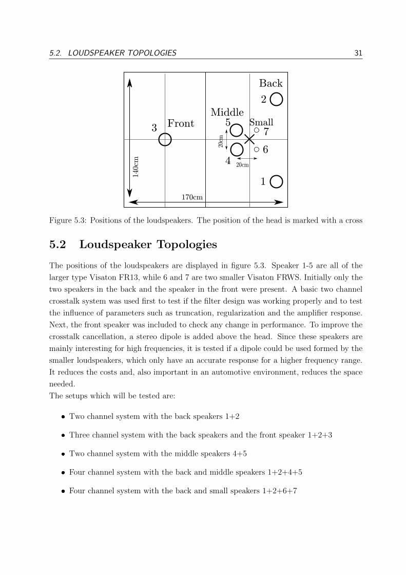
5.2. LOUDSPEAKER TOPOLOGIES 31
Figure 5.3: Positions of the loudspeakers. The position of the head is marked with a cross
5.2 Loudspeaker Topologies
The positions of the loudspeakers are displayed in figure 5.3. Speaker 1-5 are all of the
larger type Visaton FR13, while 6 and 7 are two smaller Visaton FRWS. Initially only the
two speakers in the back and the speaker in the front were present. A basic two channel
crosstalk system was used first to test if the filter design was working properly and to test
the influence of parameters such as truncation, regularization and the amplifier response.
Next, the front speaker was included to check any change in performance. To improve the
crosstalk cancellation, a stereo dipole is added above the head. Since these speakers are
mainly interesting for high frequencies, it is tested if a dipole could be used formed by the
smaller loudspeakers, which only have an accurate response for a higher frequency range.
It reduces the costs and, also important in an automotive environment, reduces the space
needed.
The setups which will be tested are:
Two channel system with the back speakers 1+2
Three channel system with the back speakers and the front speaker 1+2+3
Two channel system with the middle speakers 4+5
Four channel system with the back and middle speakers 1+2+4+5
Four channel system with the back and small speakers 1+2+6+7

32 CHAPTER 5. SYSTEM DESIGN
5.3 Plant Matrix Measurements
Characterizing the system is of utmost importance to design the compensation filters. To
determine the plant matrix, the impulse responses of different loudspeakers to both ears
were measured. When an input signal is presented to a device under test, the output can
be obtained by convolving the impulse response with the input:
y(t) = h(t) ∗ x(t) =
∫ +∞
−∞h(τ)x(t− τ)dτ (5.1)
In the frequency domain this corresponds to multiplying the input spectrum with the
transfer function:
X(f) = H(f) · Y (f) (5.2)
An impulse response can be determined by exciting each frequency and measuring the
response of the system. In theory a Dirac-pulse could be sent out which contains all
frequencies in a very short time interval. Inserting a Dirac δ function in 5.1 shows that the
impulse response is obtained instantly. However, it is in practice very hard to excite such a
pulse witch sufficient power at each frequency. For the deconvolution of the measured test
signal it is possible to use any excitation signal as long as it has enough energy in frequency
range of interest [33]. In this thesis a linear sweep was used. It excites each frequency,
starting at the lower ones, with the same amount of energy and thus the spectrum is
white. Equation 5.2 shows that the impulse response can be obtained by dividing the
spectrum of the output with the spectrum of the input signal and then using an inverse
FFT. A problem arising is that this method generates a lot of noise outside the range of
excitation. The spectrum of the input is very low outside the excited range and dividing
by this spectrum boosts these frequencies in the transfer function. Band-pass filtering can
be used to filter out this noise. Looking back at the time domain representation it can
be seen that the impulse response can also be obtained by convolving the output response
with the inverse filter of the input. For the linear sweep, the inverse filter is its time-inverse
since the spectrum is white. [33]. A convolution with a time-reversed signal is equivalent
to the cross-correlation:

5.3. PLANT MATRIX MEASUREMENTS 33
y(t) ∗ x(−t) =
∫ +∞
−∞y(τ)x(τ − t)dτ (5.3)
substituting u = τ − t
⇒ y(t) ∗ x(−t) =
∫ +∞
−∞y(t+ u)x(u)dτ (5.4)
def= Rxy(t) (5.5)
The operation is illustrated in figure 5.4. It is also advisable to switch to the frequency
domain at this point benefit from the reduced computation time due to the FFT. The
output and the inverse filter can be transformed and multiplied to obtain the transfer
function. Note that the time-inverse becomes the complex conjugate of the input in the
frequency domain.
Figure 5.4: Calculation of the impulse response for a white excitation signal [33]
Measurements were performed using a LabView interface. The test signals were sent out
using an external Terratec DMX sound card to an audio amplifier which drives the speak-
ers. A Bruel & Kjær Head and Torso Simulator was placed inside the cabin to record a
left and right ear signal. For the data acquisition a PXIe-1082 chassis with a PXIe-4498
slot from National Instruments was used. It takes the (preamplified) microphone signal
and feeds it back to LabView using an 24-bit ADC. The sampling frequency was put to
48 kHz. The linear sweep used had a duration of 60 s and ranged from 80 Hz to 8000 Hz.
The LabView program saves the input signal, but the delay to the output was not constant
each time a measurement was performed. When measuring two different speakers subse-
quently crucial phase information for the cancelling was lost. Therefore, it was decided

34 CHAPTER 5. SYSTEM DESIGN
to measure an analog voltage in the signal path and feed it back to a second input of
the PXI to use as a reference signal for the deconvolution. The voltage can be measured
at the output of the sound card allowing to include a compensation for the amplifier in
the filters. The plant matrix describing the system thus encompasses: amplifier response,
speaker response, room response and the HRTF. Since the response is part of the plant
matrix, they don’t need to be maximally flat, but a flat response relaxes the compensation
effort of the inverse filters.
5.4 Filter Design
FIR filters are designed based on the measured impulse responses in the plant matrix. The
impulse responses are band-pass filtered so any noise outside the range of excitation is
omitted. The impulse responses are truncated subsequently to 48000 samples correspond-
ing to a length of 1 s. This length allows the reverberant tail to drop below the noise floor
so no information is lost. The plant matrix is normalized to its maximum value for con-
venience. This only has an influence on the amplitude of the filters and doesn’t influence
the shape. The inverse filtering is performed in the frequency domain using 3.12, repeated
here:
C = [HHH + βI]−1HH (5.6)
This equation actually denotes a set of equations since the inversion is performed for each
frequency separately. The regularization parameter β is chosen so the length of the filter
is concentrated in the central part. An example of an inverse filter is shown in figure 5.5.
An optimal value has to be determined by trial and error but the exact value is not very
critical [27]. In this work a value of β = 0.05 was chosen. For a further improvement it
is advisable to use a frequency-dependent regularization parameter [34]. Using a single
parameter results in an attempt to equalize the response over the full frequency range.
However, the frequency bands outside the range of excitation have a low level in the
transfer function, so in the inverse filter they are boosted unnecessarily. By applying a
very large value for the regularization parameter in these regions, the inverse filters have
no energy outside the range of interest.
As a final step, the inverse filters are transformed back to the time domain and a cyclic
shift over half the length is applied. This implements a modelling delay and creates causal
filters.

5.5. AMPLIFIER DESIGN 35
0 1 2 3 4 5
x 104
−1
−0.8
−0.6
−0.4
−0.2
0
0.2
0.4
0.6
0.8
1
Samples (n)
Figure 5.5: Example of an inverse filter with its energy concentrated in the central part
5.5 Amplifier Design
5.5.1 Influence of amplifier characteristics
Initially, two types of Pioneer audio amplifiers were used to drive the speakers, a VSX-826
and a A-607R. The frequency responses of both were measured for the 80 Hz to 8000 Hz
excitation signal from the sound card and loaded with 4 Ohm. The responses are depicted
in figure 5.6. The VSX-826 has an almost perfectly flat response while the A-607R shows
a fairly big drop-off above 1 kHz. According to the specs, the response should be flat up
100 kHz so an internal component is probably failing. This is not necessarily a problem since
the amplifier characteristic can be a part of the plant matrix system and thus are equalized
as well. However, above 250 Hz the response also starts showing some modulation, probably
due to nonlinear effects in the amplifier. These nonlinearities cannot be compensated for,
since using impulse responses implies dealing with linear systems. Crosstalk will still be
possible, but as can be seen in figure 5.7, the performance for the same crosstalk system is
worse than with the other amplifier.
For this reason it was decided to build a set of new small mono amplifiers to be able to
test a multichannel set-up without having a limited performance due to the amplifier.

36 CHAPTER 5. SYSTEM DESIGN
102
103
35
40
45
50
55
Frequency (Hz)
Magnitude(dB)
A−607RVSX−826
Figure 5.6: Frequency responses of the Pioneer amplifiers. (The absolute value of the
magnitude has no significance.)
102
103
−60
−40
−20
0
20
40
60
Frequency (Hz)
Magnitude(dB)
LeftRight
(a)
102
103
−60
−40
−20
0
20
40
60
Frequency (Hz)
Magnitude(dB)
LeftRight
(b)
Figure 5.7: Comparison of the two channel crosstalk cancellation with the two different
Pioneer amplifiers. Measurements happened subsequently with the HATS at the same
position. A two channel system with speaker 1 and 2 in the back was used.

5.5. AMPLIFIER DESIGN 37
5.5.2 Circuit
The amplifier chip which was initially chosen is the TDA2050 from STMicroelectronics.
It is an audio class AB amplifier suited for hi-fi applications. It can deliver a high output
power over a wide range of input voltages and can be used with a single supply voltage.
This allows it to be used with a commercially available laptop power supply for example
and omits the need of including a dedicated power supply circuit. With a 20 V single supply
voltage the amplifier is able to deliver 5 W to an 8 Ohm load -the small speakers- and 8 W
to a 4 Ohm load -the big speakers- at which is more than sufficient for playback in the cabin.
The influence of the external components will be discussed next and simulated when pos-
sible. The amplifier is modelled in PSpice (cfr. figure 5.8) by an ideal op-amp and the
loudspeaker is modelled as a resistance in series with an inductor. The values correspond
to those from the FRWS 5 SC speaker.
Figure 5.8: PSpice simulation circuit
Bias Network
The power supply provides a bias voltage at the input of the amplifier. At DC we can
consider the capacitors to be open circuits. R1 and R2 form a resistive voltage divider
and since they are equal, the bias voltage will be half of the supply voltage. The input
impedance of the op-amp can be considered very high so no currents flow through R3 and
the bias voltage is produced at the non-inverting input. In the circuit the DC voltages are

38 CHAPTER 5. SYSTEM DESIGN
shown and verify the prediction. The power supply is decoupled for AC by C3 and C5.
These form the common combination of a larger capacitor able to store more energy and
a smaller one with a good high frequency response.
Input
At the input it is necessary to block DC-voltages because these would decrease the dynamic
range of the amplifier or even cause saturation. In a first approximation we can consider
C2 to be a short circuit at AC and since C2 is connected in parallel with R1 and R2 we
can also neglect the influence of these resistors. R3 is then connected to ground and a first
order high-pass filter, formed by C1 and R3, is present at the input. The cutoff frequency
can be found as:
fc =1
2πR3C1
=1
2π 2.2µF 22kΩ= 3.3 Hz (5.7)
Using the above value the assumptions about the other components can be checked. The
impedance of capacitor C2 at the cutoff frequency is:
Z =1
2πfcC2
=1
2π 3.3Hz 100µF= 482 Ω (5.8)
When put in parallel with two resistors of 22 kΩ, this leads to an impedance of 462 Ω. So
neglecting the two resistors only gives a minimal difference of less than 5%. In series with
a 22 kΩ resistor, the 482 Ω impedance is added so a total resistance of 22 482 Ω is obtained.
Neglecting the influence of the capacitor again results in a difference of less than 5% so the
assumption of R3 connected to ground is justified as well. The input transfer function is
simulated and depicted in figure 5.9a. The −3 dB mark appears to be close to 3 Hz as was
predicted.
Gain
The gain is determined by the feedback network formed by R4, R5 and C4. The non-
inverting amplifier topology has following transfer function:
G = 1 +R5
R4 + 1jωC4
= 1 +jωR5C4
jωR4C4 + 1(5.9)
≈ 1 +R5
R4
for high frequencies (5.10)
≈ 1 +22 kΩ
680 kΩ(5.11)
≈ 30.5 dB (5.12)

5.5. AMPLIFIER DESIGN 39
It is clear that the gain is mainly influenced by the R5-R4 ratio. The low-frequency cutoff
is determined by the R4-C4 combination and can be found as:
fc =1
2πR4C4
=1
2π 22µF 680Ω= 10.6 Hz (5.13)
The main reason for this high-pass filtering is to provide a proper DC-bias at the output
of the amplifier. At DC R4 is decoupled and R5 is the only component left in the feedback
path. This connects the output back to the input and results in unity gain. As a conse-
quence, the DC-bias at the input is reproduced at the output. The transfer function can
again be verified in PSpice (cfr. figure 5.9b).
Output
Since DC voltages could damage a loudspeaker, it is necessary to prevent them from going
to the output. C7 is a blocking capacitor which forms a high-pass filter together with the
resistance of the speaker. For an 8 Ohm speaker this becomes:
fc =1
2π 1000µF 8Ω= 20 Hz (5.14)
This is also observed when looking at the simulated transfer function from the output of
the amplifier to the speaker input in figure 5.9c.
There is also a Zobel-network present at the output, formed by R6 and C6. Since loud-
speaker impedances are generally inductive at higher frequencies because of the voice-coil
impedance, the load of the amplifier increases with frequency. A Zobel-network tries to
compensate for that by introducing a series RC combination in parallel with the output.
By choosing R6 equal to the loudspeaker impedance RLP and C6 = LLP/R2LP the am-
plifier would always see purely resistive load equal to the loudspeaker impedance. Since
a better model for a voice-coil would be a lossy inductor rather than an ideal one, some
more complicated calculations can be made [35]. Keeping an exact resistive value for the
load is mainly important when designing (passive) crossover networks. For the amplifier
it is important to maintain stability at higher frequencies and the Zobel-network can be
considered to be a low-pass filter. The recommended values in the datasheet introduce a
pole around 150 kHz to prevent ultrasonic oscillations.
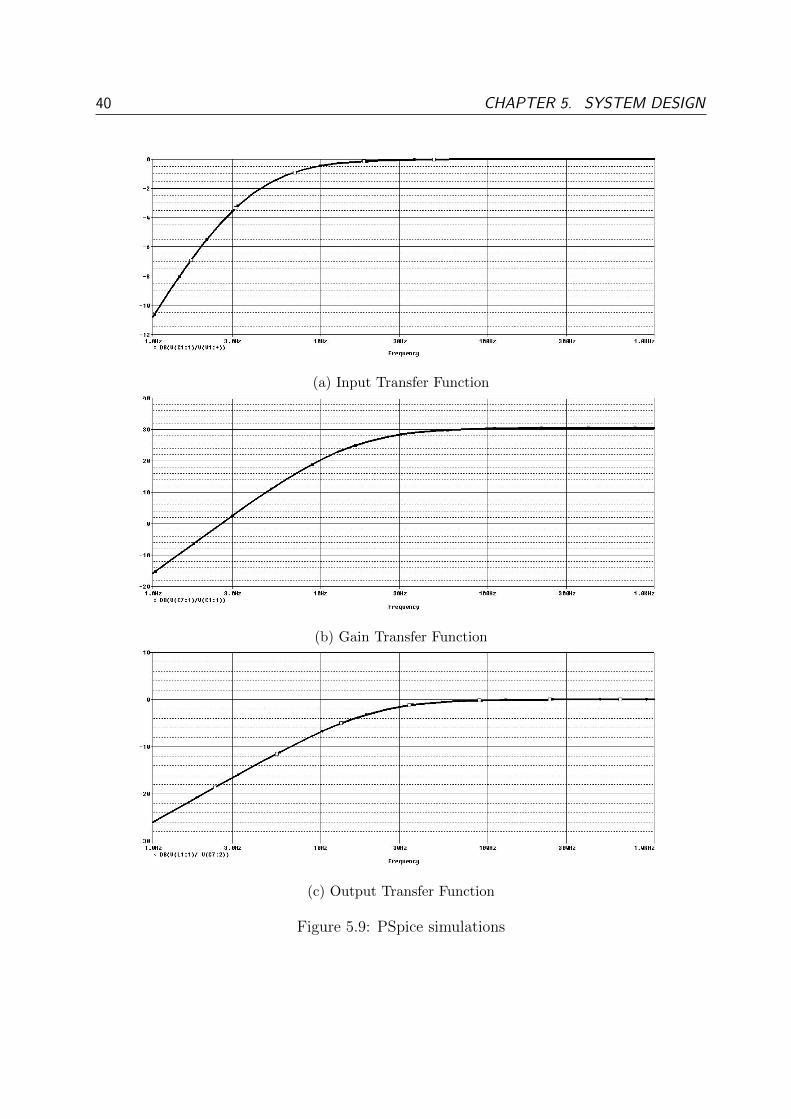
40 CHAPTER 5. SYSTEM DESIGN
(a) Input Transfer Function
(b) Gain Transfer Function
(c) Output Transfer Function
Figure 5.9: PSpice simulations

5.5. AMPLIFIER DESIGN 41
Second Design
A second design is made using an LM3875 amplifier chip from Texas Instruments. This
chip can be embedded with almost identical external components, but outperforms on
properties such as output power, distortion and noise floor. The LM3875 is able to deliver
up to 56 W into an 8 Ohm load at a distortion of 0.1%, while the TDA2050 can maximally
deliver 32 W into an 8 Ohm load at a distortion of 10%. The EAGLE schematic in figure
5.10 shows the final amplifier circuit. A series RC circuit with a pole around 150 kHz is
added in shunt with the feedback path. This lowers the gain at high frequencies and thus
increases the phase margin. Also a small capacitor is added across the input pins of the
amplifier. This capacitor forms a low-pass filter with the source impedance again to avoid
high frequency oscillations. Currents from the output lead could be coupled to the input
when the source impedance is high. The higher the source impedance, the lower the cutoff
frequency of the filter.
Figure 5.10: EAGLE schematic
5.5.3 Board design
EAGLE was used to make a PCB design. The schematic and layout design are depicted
in figures 5.10 and 5.11. The limited number of components made it possible to limit the
board to a one-layer design. The copper layer and the SMD components were put on the
bottom layer so through-hole components could be placed on the top. Screw terminals
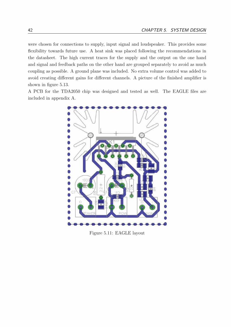
42 CHAPTER 5. SYSTEM DESIGN
were chosen for connections to supply, input signal and loudspeaker. This provides some
flexibility towards future use. A heat sink was placed following the recommendations in
the datasheet. The high current traces for the supply and the output on the one hand
and signal and feedback paths on the other hand are grouped separately to avoid as much
coupling as possible. A ground plane was included. No extra volume control was added to
avoid creating different gains for different channels. A picture of the finished amplifier is
shown in figure 5.13.
A PCB for the TDA2050 chip was designed and tested as well. The EAGLE files are
included in appendix A.
Figure 5.11: EAGLE layout

5.5. AMPLIFIER DESIGN 43
5.5.4 Test
The frequency response for both the TDA2050 and the LM3875 pcb was measured over a
20 to 20 kHz range for a 4 Ohm load impedance. The results are shown in figure 5.12. Both
amplifiers have a nearly flat response up to the high frequencies. The cutoff frequency is
around 40 Hz as predicted by equation 5.14 for a 4 Ohm load. The shape of the response
is the same for both amplifiers, indicating that it is primarily influenced by the external
components. The TDA2050 appears to be noisier than the LM3875 chip, though the 50 Hz
component of the power net is coupled more strongly in the latter. As can be seen the
next chapter, the amplifier perform good when used for the crosstalk cancellation system.
102
103
104
15
20
25
30
Frequency (Hz)
Magnitude(dB)
Figure 5.12: Amplifier frequency response. The absolute value of the magnitude has no
significance

44 CHAPTER 5. SYSTEM DESIGN
Figure 5.13: Finished amplifiers

Chapter 6
Results
This chapter covers the objective performance of the designed crosstalk cancellation system.
Filtered test signals were played back in the cabin and recorded with the HATS to measure
the quality of the crosstalk cancellation. Typical figures of merit are channel separation,
sweet spot size and spectral distortion. Binaural signals can be played back after being
filtered with the crosstalk filters and the quality of the reproduction can be quantified by
calculating the interaural differences.
6.1 Crosstalk Cancellation Quality Measures
The test setup used is similar to the one used for the determination of the plant matrix.
Signals can be filtered and played back in MatLab using the open source C library Portaudio
and an ASIO driver. ASIO allows to address the hardware directly, in this case the Terratec
sound card, and root the different channels to the corresponding outputs. The sound
is recorded with the HATS and the data is acquired in LabView through the National
Instruments data acquisition system.
Channel Separation
The goal of a crosstalk cancellation system is essentially to perfectly control which amount
of sound is sent to one ear without influencing the sound at the other ear. A criteria to
quantify this is the channel separation. When a signal is sent to one channel of the crosstalk
filters and nothing to the other, the ratio of the recorded sound level at the ipsilateral ear
to the sound level at the contralateral ear then allows to evaluate the performance. For
the tests a linear sweep is sent to the left channel, so ideally one would recover the sweep

46 CHAPTER 6. RESULTS
exactly at the left ear and record silence at the right ear. So if no directional cues are
attached to the emitted signal, the listener is not able to give a direction to that sound.
He only hears the original monaural sweep at the left ear and nothing at the right ear. In
practice this will be impossible to achieve and some crosstalk will always be present. The
system in the cabin is designed and tested for a frequency range of 80 Hz to 8000 Hz.
Sweet Spot
In a virtual 3D environment the sound is only reproduced at the spot of the ears. The
crosstalk filters are designed for a specific listening position and changing this position
results in a decrease in performance. An automotive listening situation has the advantage
that the position of the driver is known in advance, in contrast to applications where the
listener can freely move around. The driver can still move his head in a limited area in
which the performance deteriorates with respect to the optimal position. In the tests, only
the rotational sweet spot is considered. The channel separation up to an angle of 30 degrees
will be looked at. Since the listening situation is not perfectly symmetrical, rotations to
the left and right side will yield slightly different results. However, this will provide no
new insights so only the sweet spot for rotations to one side will be looked at. A dynamic
system could improve the sweet spot by adapting the filters to the position of the head.
Distortion
It is not only important to present the correct interaural differences to a listener, but it
is also desired to preserve the monaural characteristics of the sound. A sound system
tries to reproduce music without adding any spectral coloration which could change the
music experience. Moreover, in a binaural reproduction system, distortion could change
the spatial information contained in the spectral cues.
As a reference, the response measured with the HATS for a linear sweep through the left
loudspeaker in the back without any filtering is shown in figure 6.1. The shape of an HRTF
as in 2.2 can be recognized by the resonance of the ear canal at 2 kHz. The many sharp
peaks and dips show the big influence of the cabin environment. Unlike in the case of an
anechoic HRTF, there is no natural channel separation. At certain frequency ranges the
level at the contralateral ear is even higher than at the ipsilateral ear.

6.1. CROSSTALK CANCELLATION QUALITY MEASURES 47
102
103
−80
−70
−60
−50
−40
−30
−20
−10
0
10
20
Frequency (Hz)
Magnitude(dB)
LeftRight
Figure 6.1: Measured HATS-response from the left loudspeaker in the back without
crosstalk cancellation filtering
6.1.1 Visualization using 1/3 Octave Bands
The crosstalk cancellation results a rapidly varying response at the contralateral ear and
thus also results in cumbersome data for the channel separation. To reduce the resolution
and to be able to make comparisons between different sets, the frequency range is divided
into 1/3 octave band and the energy is calculated per band. The center frequencies for the
bands are spaced as
fn+1 =3√
2fn (6.1)
and feature a constant relative bandwidth. The bands are centered at 1000 kHz and are
given in B. The 80 and 8000 Hz bands are at the limit of the excited range so the value
is not fully valid. However, based on a more narrow band analysis, the level gives a good
indication of the channel separation so it is decided to include the outer bands in the plots.
An example is shown in 6.2. This approach is justified since the human auditory system
doesn’t have an infinite resolution either. An energy integration is performed in bands
much alike 1/3 octave bands [6].

48 CHAPTER 6. RESULTS
102
103
−40
−30
−20
−10
0
10
20
30
40
50
60
Frequency (Hz)
Chan
nel
Sep
aration
(dB)
Original data1/3 Octave band analysis
Figure 6.2: Comparison of the original channel separation and the 1/3 octave band average
6.2 System performance: Channel Separation and Sweet
Spot
The playback results for the static crosstalk cancellation system, for the different loud-
speaker topologies mentioned in the previous chapter, are shown in figures 6.3 - 6.6. For
each topology, the measured response at the ears for the linear sweep through the left
channel is displayed, as well as the channel separation for different angles of rotation while
keeping the inverse filters for the initial head orientation. The plant matrix was remea-
sured each time before a set of measurements to exclude errors from the positioning of the
HATS.
The first setup which was tested, was the two channel system using only speakers 1 and 2 in
the back. The crosstalk filters perform already pretty good at the central position. Above
200 Hz a channel separation of 18 to 25 dB achieved in the 1/3 octave bands. When the
head is rotated, the performance quickly decreases. The deterioration is quicker and more
severe for higher frequencies. This can be expected since the cancelling sound waves create
interference patterns with a spacing proportional to the wavelength. Rotating the head
can then more easily bring the ears from a maximum to a minimum or vice versa. This can
even lead to a larger amount of sound received at the right ear than at the left ear as is for

6.2. SYSTEM PERFORMANCE: CHANNEL SEPARATION AND SWEET SPOT 49
example the case for the 1/3 octave band centered at 2500 Hz. From the response at the
ears, it can been seen that the crosstalk cancellation is hard to realize at certain discrete
frequencies. These are the frequencies at which the inversion-problem is ill-conditioned.
This typically happens at frequencies where the measured transfer functions are almost
equal for both ears. The plant matrix is then almost singular, so a good inversion is hard
to obtain. It can be seen for example that the resonance peak of the cabin around 130 Hz
is hard to control. Small errors can also be introduced due to noise or non-stationarity of
the plant matrix.
In the next step, the front loudspeaker is added so now the filtering happens through a
three channel system. Figure 6.4 shows that the overall performance is improved by inclu-
sion of a third loudspeaker. The channel separation is now in the range of 18 to 30 dB in
the 1/3 octave bands from 200 Hz onwards. The response also shows the number of dis-
crete frequencies at which inversion is hard to realize is strongly reduced due to an added
degree of freedom. The rotational sweet spot is not increased much however. The response
decreases in a similar way to the two channel setup. This indicates that simply adding
loudspeakers will not necessarily result in an improvement of the sweet spot, so a careful
choice of the position should be taken into account.
As already mentioned in the previous chapter, a stereo dipole pair is tested as well. Pre-
vious research shows that this setup can realize a broad sweet spot at higher frequencies
at expense of a reduction in performance at the lower frequencies. The stereo dipole is
formed by the two middle speakers located above the head. The plots in figure 6.5 verify
the expected behavior. The performance of the crosstalk cancellation at the central posi-
tion is a lot worse than with the previous setups, but a clear improvement in the sweet
spot for frequencies above 2 kHz is achieved.
In a last setup, a four channel systems is tested which tries to combine the asset of two
setups. The system with the two back speakers has a good performance for low frequencies
but suffers from strong reduction at high frequencies when the head is rotated, whereas the
two middle speakers have a reduction in performance at the low frequencies while having
a broader sweet spot for high frequencies. The results are shown in figure 6.6. Crosstalk
cancellation is achieved over the full frequency range in the central position. From the
200 Hz band onwards the cancellation doesn’t drop below 21 dB matching the performance
of common systems in anechoic environments [23]. The response shows that the four
channel system doesn’t suffer from discrete frequencies at which the inversion cannot be
realized. The sweet spot is increased by including the middle speakers in comparison with
the the system only using the back speakers.
To have an overview of the performance of the systems, the results at the central position

50 CHAPTER 6. RESULTS
and at an angle of 30 degrees are plotted together for the different topologies in figure 6.7.
It is clear that the four channel system has the best overall performance and manages to
combine the assets of the middle and back loudspeaker positions.
A further improvement could consist of implementing a dynamic crosstalk cancellation sys-
tem. A head tracker would then need to be included to detect the position of the head and
update the plant matrix accordingly. Figure 6.8 shows the channel separation for a head
rotation of 30 degrees when the plant matrix is adapted to the orientation. The results for
the two channel system, using speaker 1+2, and the three channel system are compared
with the performance of the static crosstalk canceller for the 0 and 30 degrees rotation. It
can be seen that updating the plant matrix for the rotated head allows a gain of more than
20 dB for the highest frequencies. For the two channel system, the matched plant matrix
at 30 degrees has a decrease in performance up to 8 dB compared to the matched plant
matrix at 0 degrees. This caused by different positions of the loudspeakers if rotated. In
the limiting case of a rotation of 90 degrees, both loudspeaker are placed at one side of the
head, so it is hard to control the sound at the ear directed away from the speakers. The
three channel system doesn’t suffer from this problem since at least one speaker is always
placed one side of the ears. The plot shows that the plant matrix at 30 degrees results in
a comparable performance with the plant matrix for 0 degrees.

6.2. SYSTEM PERFORMANCE: CHANNEL SEPARATION AND SWEET SPOT 51
102
103
−60
−40
−20
0
20
40
60
Frequency (Hz)
Magn
itude(dB)
LeftRight
(a) Response at the two ears (0°)
102
103
−20
−10
0
10
20
30
40
Frequency (Hz)
Channel
Separation
(dB)
0°10°20°30°
(b) Channel separation for different angles
Figure 6.3: Two channel system with back speakers

52 CHAPTER 6. RESULTS
102
103
−60
−40
−20
0
20
40
60
Frequency (Hz)
Magn
itude(dB)
LeftRight
(a) Response at the two ears (0°)
102
103
−20
−10
0
10
20
30
40
Frequency (Hz)
Chan
nel
Sep
aration(dB)
0°10°20°30°
(b) Channel separation for different angles
Figure 6.4: Three channel system with back speakers and front speaker

6.2. SYSTEM PERFORMANCE: CHANNEL SEPARATION AND SWEET SPOT 53
102
103
−60
−40
−20
0
20
40
60
Frequency (Hz)
Magn
itude(dB)
LeftRight
(a) Response at the two ears (0°)
102
103
−20
−10
0
10
20
30
40
Frequency (Hz)
Chan
nel
Sep
aration(dB)
0°10°20°30°
(b) Channel separation for different angles
Figure 6.5: Two channel system with middle speakers

54 CHAPTER 6. RESULTS
102
103
−60
−40
−20
0
20
40
60
Frequency (Hz)
Magn
itude(dB)
LeftRight
(a) Response at the two ears (0°)
102
103
−20
−10
0
10
20
30
40
Frequency (Hz)
Chan
nel
Sep
aration(dB)
0°10°20°30°
(b) Channel separation for different angles
Figure 6.6: Four channel system with back speakers and middle speakers

6.2. SYSTEM PERFORMANCE: CHANNEL SEPARATION AND SWEET SPOT 55
102
103
−20
−10
0
10
20
30
40
Frequency (Hz)
Chan
nel
Separation
(dB)
Back LPBack+Front LPMiddle LPBack+Middle LP
(a) Channel separation when the head is not rotated
102
103
−20
−10
0
10
20
30
40
Frequency (Hz)
Channel
Sep
aration
(dB)
Back+Middle LPMiddle LPBack+Front LPBack LP
(b) Channel separation at an angle of 30 degrees
Figure 6.7: Comparison of channel separation and sweet spot for different loudspeaker
topologies

56 CHAPTER 6. RESULTS
102
103
−20
−10
0
10
20
30
40
Frequency (Hz)
Chan
nel
Separation
(dB)
30° dynamic CTC0°30° static CTC
(a) Comparison of the channel separation with dynamic and static crosstalk cancellation
for the two channel setup
102
103
−20
−10
0
10
20
30
40
Frequency (Hz)
Chan
nel
Sep
aration(dB)
30° dynamic CTC0°30° static CTC
(b) Comparison of the channel separation with dynamic and static crosstalk cancellation
for the three channel setup
Figure 6.8: Comparison of channel separation and sweet spot for different loudspeaker
topologies

6.3. SYSTEM PERFORMANCE: DISTORTION 57
6.3 System performance: Distortion
The frequency response at the left ear can be used to get an impression of the distortion in
the system. Since a linear sweep is used as an excitation signal, a system without distortion
would result in a perfectly flat response at the ear. Distortion occurs at frequencies at
which it is hard to realize the equalization of the plant matrix. Figure 6.9a shows the
shifted frequency responses for the different loudspeaker topologies at the central position.
The four channel system has the better crosstalk cancellation performance and thus also
has the least distortion. When the head is rotated, the performance decreases at higher
frequencies and this also introduces more distortion. Sharp notches and peaks are noticed
due to interference patterns. When the sweet spot is larger, these notches and peaks are
less present, so there is also less distortion. The responses at an angle of 30 degrees are
shown in 6.9b. Again the four channel system proves to result in the best performance.
When compared with the reference response in figure 6.1, the crosstalk cancellation results
in a major improvement in the distortion by equalizing the room response.
6.4 Performance with Small Loudspeakers
The four channel system showed the best performance by increasing the sweet spot at
higher frequencies by including a stereo dipole. This leads to the idea that the stereo
dipole speakers could be replaced by smaller speakers which only have a good frequency
response at higher frequencies. Figure 6.10 shows the results for a four channel system with
the smaller loudspeakers 6,7 and the back speakers 1,2. A very good channel separation
for the central position is noted, but there is almost no improvement in the sweet spot size
compared to the two channel system. This indicates that the cancellation is dominated by
the two back speakers. The small speakers have a lower power response than the bigger ones
so an equal contribution of the two types would require higher energy filters for the former.
The plant matrix takes level differences into account, but the inversion also limits the
energy in the filters. There is a trade-off between having a better performance, with more
energy sent to the smaller speaker, and less energy when mainly using the larger speakers
with a reduced performance. To improve the sweet spot one could maybe try to force
more energy in the smaller filters by introducing some channel-dependent regularization,
but this possibility was not explored any further. Another possible cause for the reduced
performance, could be different position of the stereo dipole. It is more to the back towards
the other speakers, compared to the original stereo dipole. The four speaker are then at
the same side of the head, so this topology could result in a more limited performance.

58 CHAPTER 6. RESULTS
102
103
−60
−40
−20
0
20
40
60
Frequency (Hz)
Magn
itude(dB)
Back LPBack+Front LPMiddle LPBack+Middle LP
(a) Frequency response at the left ear at an angle of 0 degrees
102
103
−60
−40
−20
0
20
40
60
Frequency (Hz)
Mag
nitude(dB)
Back LPBack+Front LPMiddle LPBack+Middle LP
(b) Frequency response at the left ear at an angle of 30 degrees
Figure 6.9: Comparison of the frequency responses for different loudspeaker topologies to
illustrate distortion

6.4. PERFORMANCE WITH SMALL LOUDSPEAKERS 59
102
103
−20
−10
0
10
20
30
40
Frequency (Hz)
Chan
nel
Separation
(dB)
(a) Channel separation for different angles
102
103
−20
−10
0
10
20
30
40
Frequency (Hz)
Channel
Separation
(dB)
Back+Small LPBack+Middle LPBack+Small LP 30°Back+Middle LP 30°
(b) Comparison of the two four channel setups
Figure 6.10: Four channel system with back speakers and small speakers

60 CHAPTER 6. RESULTS
6.5 Performance for Shorter Filters
A real time crosstalk canceller was previously developed at Intec Acoustics. The filtering
was based upon at database of HRTFs measured in an anechoic environment. The challenge
for integration with the current filters is that the transfer functions measured in the cabin
are a lot longer due to the reverberant environment. A length up to 1 s is needed before
the reverberant energy in the impulse response drops below the noise floor. In contrast
a measured HRTF in an anechoic chamber can be truncated until it has a duration of
only 11.6 ms. The real-time filtering is done in the frequency domain so the computation
speed depends on the block length of the FFT. Testing the application shows that 16384 is
the maximum block length that can be handled by the computer that is used. Increasing
the block length even further, results in audible artifacts because the computations do
not happen fast enough to fill the output buffer. The current filters have a length of
48000 samples so are not suited for the real-time application. Too shorten the filters, the
measured impulse responses could be truncated to 15000 samples before being inverted. A
decrease in performance can be expected since some relevant data in the impulse response
is cut away and generally also because the filter has a lower order. Figure 6.11 shows
the performance for two setups compared to the original filters. A slight reduction in the
channel separation can be noted. The four channel system suffers slightly less from the
reduction in filter length and proving another asset for this system. The maximum loss
is 4.5 dB for the four channel system while it is 5.5 dB for the two channel system. The
regularization parameter can be used to control the duration of the filters, but choosing
the regularization parameter higher than necessary results a strongly reduce performance,
before a substantial reduction in filter length is achieved. So it not advisable to use this
approach to get shorter filters. Moreover, in the current implementation, the inverse filters
are calculated in real-time and thus the inversion operation is a limiting factor. Shortening
the inverse filters will not gain much speed.
6.6 3D Sound Virtualization
Crosstalk cancellation was introduced as a technique to deliver binaural signals to the ears.
To create a 3D illusion, it is important that the spatial cues in the signals are preserved.
When the channel separation is not high enough, the binaural signals are deformed and
a wrong source position is perceived. In [36] a channel separation of 12 dB is stated as
sufficient to produce accurate virtual sources. However, in [37] a minimum value of 15 dB
to 20 dB is indicated, so the limit is implementation-dependent. As became clear in section

6.6. 3D SOUND VIRTUALIZATION 61
102
103
−20
−10
0
10
20
30
40
Frequency (Hz)
Channel
Separation(dB)
1500048000
(a) Two channel system with back speakers
102
103
−20
−10
0
10
20
30
40
Frequency (Hz)
Channel
Separation(dB)
4800015000
(b) Four channel system with back speakers
and middle speakers
Figure 6.11: Performance for shorter filters
2.1, many cues contribute to the sound localization mechanism in the auditory system. To
estimate the quality of the 3D reproduction, only the interaural level and time differences
are used. Binaural synthesis was performed using HRTFs from the CIPIC dataset [9] to
add spatial information to monaural music sample. The binaural signals were played back
in the cabin after being filtered with the crosstalk cancellation filters. The signals recorded
with the HATS can then be compared with the original binaural signals to estimate the
quality of the reproduction.
The ITD can be estimated by calculating the interaural cross-correlation between the left-
ear signal and the right-ear signal [38]. The time difference is then found as the time where
the cross-correlation is maximized. The threshold for untrained listeners to discriminate
differences in ITD at a frequency of 0.5 kHz [39]. This value can be used as a reference to
quantify the reproduction.
The ILD can be calculated by taking the ratio of the energy spectrum of the two binaural
signals:
ILD = 10(log)
f2∫f1
|Xleft(f)|2 df
f2∫f1
|Xright(f)|2 df
(6.2)
The integration range is chosen from 1 kHz to 5 kHz since in this region the ILD is a primary
62 CHAPTER 6. RESULTS
cue for localization [40]. As a reference, a threshold for discrimination between differences
in ILD is around 4 dB at 4 kHz for untrained listeners [39].
The generated virtual sources lie in the horizontal plane at following angles angles: 0°, 10°,
20°, 30°, 45° and 65°. The 0° source indicates a spot directly ahead of the listener, while
increasing angles indicate sources displaced to the right. Only sources in the horizontal
plane are considered since the interaural cues mainly provide spatial information in this
plane [6].
In table 6.1 and 6.2 the results are compared for the two channel system using loudspeakers
1+2 in the back and the four channel system also including loudspeaker 4+5 in the middle.
The differences are measured when the head is in the optimal position at an angle of 0
degrees and when the head is rotated over 30 degrees. At the optimal listening position
the reproduction of the ITD is nearly perfect for both systems. Only for the source at 10°
a difference is measured, but it is below the discrimination threshold. When the head is
rotated, the performance of the crosstalk cancellation is worse so the reproduction of the
ITD is less good. For the two channel system, differences occur up to almost 400µs and
the spatial information in the ITD cue will be lost. The four channel system provides a
broader rotational sweet spot and it can be seen that this results in lower differences in the
ITD. It can be seen that differences are just below or above the threshold, so the spatial
information is likely to be preserved.
For the ILD the results are again very good in the optimal listening position. The dif-
ferences are not higher than 1.1 dB which is below the threshold of 4 dB. For the head
rotated to 30 degrees, the differences are a lot higher. The increase in performance of
the four channel system is not enough in the frequency range which determines the ILD.
Previous research showed that, when the cues are conflicting, the ITD cue dominates over
the ILD cue [8]. Thus, for a broadband source, will be perceived correctly with the four
channel system.
It is clear from the results that a matched plant matrix results in a very good reproduction
of the interaural cues. When a dynamic crosstalk system is used which adapts the plant
matrix to the head position, it can be expected that ITD and ILD will be preserved for
other positions than the optimal listening position.

6.6. 3D SOUND VIRTUALIZATION 63
Source position 2 channel 4 channel
0° 0 µs 0 µs
10° 21 µs 21 µs
20° 0 µs 0 µs
30° 0 µs 0 µs
45° 0 µs 0 µs
65° 0 µs 0 µs
(a) Head rotation 0°
Source position 2 channel 4 channel
0° 125 µs 42 µs
10° 228 µs 63 µs
20° 292 µs 84 µs
30° 375 µs 42 µs
45° 292 µs 62 µs
65° 354 µs 62 µs
(b) Head rotation 30°
Table 6.1: Differences in ITD when crosstalk cancellation is performed with the two channel
system (LP 1-2) and the four channel system (LP 1-2 + 4-5) for the head in the optimal
position at 0° and for a head rotation of 30°
Source position 2 channel 4 channel
0° 0.27 dB 0.17 dB
10° 0.33 dB 0.36 dB
20° 0 dB 0.2 dB
30° 0.5 dB 0.4 dB
45° 0.8 dB 0.3 dB
65° 1.1 dB 0.5 dB
(a) Head rotation 0°
Source position 2 channel 4 channel
0° 0.16 dB 7.5 dB
10° 4.87 dB 12.2 dB
20° 11.7 dB 11.0 dB
30° 17.2 dB 17.54 dB
45° 19.4 dB 19.13 dB
65° 23.3 dB 21.2 dB
(b) Head rotation 30°
Table 6.2: Differences in ILD when crosstalk cancellation is performed with the two channel
system (LP 1-2) and the four channel system (LP 1-2 + 4-5) for the head in the optimal
position at 0° and for a head rotation of 30°

64 CHAPTER 6. RESULTS

Chapter 7
Conclusion
In this thesis the possibility of creating virtual 3D audio in a vehicle environment is in-
vestigated. Binaural signals can be used, but for this it is necessary to be able to control
the sound at the ears of a listener. Measurements in the cabin show that the sound field
is heavily influenced by the environment. Reflections and resonances result in spectral de-
formation of the sound and absence of natural channel separation. The desired control is
obtained with the use of the crosstalk cancellation technique. The unwanted contribution
from a loudspeaker at the contralateral ear is cancelled with sound from a second speaker.
The impulse responses from the loudspeakers to the ears are measured in the cabin and
used for the design of an inverse filter matrix. An exact inverse is not realizable, so approx-
imated filters are calculated using a least squares method combined with a regularization
parameter.
A channel separation above 18 dB in the 200 Hz to 8 kHz range was already obtained at
the central position using a classic two channel system, approaching the performance of
20 dB of common systems in anechoic environments [23]. When the head was rotated,
the performance quickly decreased above 1 kHz, indicating a limited sweet spot. It was
tried to improve the system by implementing a multichannel loudspeaker system. A set of
small audio amplifiers was built to guarantee an identical amplification for each channel and
overcome problems with combining commercial amplifiers. Different multichannel crosstalk
cancellation systems have been investigated. The results for the three loudspeaker setup
showed that channel separation can be improved by increasing the number of transducers,
but the increase in sweet spot was limited. Additional loudspeakers were added in a specific
topology. Two closely spaced loudspeakers, forming a stereo dipole, were mounted above
the head. Crosstalk cancellation with these two speakers provides a broad rotational sweet
spot at high frequencies while it has a bad performance at low frequencies, confirming

66 CHAPTER 7. CONCLUSION
what is written in literature [29]. A four channel system was designed, combining the
stereo dipole with the initial two channel system. This results in a channel separation over
21 dB above 200 Hz and an increased sweet spot due to the two closely spaced speakers. A
dynamic crosstalk could prove to be a major improvement for the sweet spot by updating
the plant matrix according to the head position. A multichannel system is preferred since
this allows to have at least one loudspeaker at each side of the head. However, a head-
tracker needs to be included to update the plant matrix.
The crosstalk cancellation also has the asset of equalizing the room response, causing a
less distorted sound at the ears. The more crosstalk cancellation is achieved, the more flat
is the response. This implies that more distortion is present when the head is rotated. To
minimize the distortion, the four channel system proves to be the best choice.
Since the stereo dipole is meant to increase the high frequency performance, it is tested if
smaller loudspeakers can be used, which don’t need to have a response extending to the low
frequencies. Results show that the channel separation is not as good as for the regular four
channel system. Almost no improvement in the rotational sweet spot is noticed compared
to the two channel system, so it is thought that the sound field is dominated by the larger
speaker due to the higher output power. For future work it could be considered to look at
a way to increase the relative amount of energy going to the small speakers, for example
by introducing a channel-dependent regularization parameter. It also possible that the
different positioning of the speakers influence the performance negatively.
The capability of rendering virtual 3D sound is tested by synthesizing virtual sources and
playing back the binaural signals in the cabin using the crosstalk cancellation systems. To
quantify the 3D reproduction, the differences in ITD and ILD between the original binau-
ral signals and the reproduced signals at both ears are calculated for a number of source
positions. A comparison between the two channel and the four channel systems showed
that both spatial cues are preserved for the optimal listening position. The differences
are below the discrimination thresholds for untrained listeners. When the head is rotated
over an angle of 30 degrees, the differences become higher. Neither of the cues can be
reproduced correctly by the two channel setup. The four channel setup renders differences
in ITD which are close to the threshold, so the spatial information is likely to be preserved.
It is not capable of reproducing the correct ILD, indicating that the increase in rotational
sweet spot is not sufficient at higher frequencies. Since the ITD dominates ILD, broadband
sources will still be perceived correctly [8]. The human hearing is a complex process com-
prising not only the interaural differences. Physics, but also psychoacoustic effects play an
important role. Therefore, future work should include subjective experiments with listen-
ers judging the capability of creating virtual 3D sources and comparing the sound quality

67
of the systems. In the crosstalk implementation in a car by Farina [3], a 10 dB channel
separation is already sufficient to outperform a traditional audio system in subjective tests.
Another aspect to be looked at, is the integration of the designed filters in the real-time
application. Tests showed that the length of the filters can be reduced at the expense of a
small reduction in performance. Informal tests with these filters showed real-time filtering
can be executed without artifacts, but tests need to be done to validate if the filtering
is performed correctly. Other ways of reducing the filter length could be investigated as
well. A passive optical head tracker, compatible with the real-time software, was found.
The head-tracker can be included in the real-time system to create a dynamic crosstalk
cancellation system, further improving the virtual 3D environment.

68 CHAPTER 7. CONCLUSION
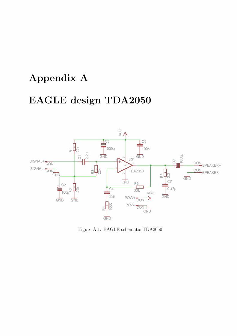
Appendix A
EAGLE design TDA2050
Figure A.1: EAGLE schematic TDA2050

70 APPENDIX A. EAGLE DESIGN TDA2050
Figure A.2: EAGLE layout TDA2050

Appendix B
1/3 Octave Bands
fl (Hz) f0 (Hz) fu (Hz)
70.8 80 89.1
89.1 100 112
112 125 141
141 160 178
178 200 224
224 250 282
282 315 355
355 400 447
447 500 562
562 630 708
708 800 891
891 1000 1122
1122 1250 1413
1413 1600 1778
1778 2000 2239
2239 2500 2818
2818 3150 3548
3548 4000 4467
4467 5000 5623
5623 6300 7079
7079 8000 8913


Bibliography
[1] Auro-Technologies, “Auro-3d.” http://www.auro-technologies.com.
[2] SRS, “Car audio.” http://www.circlesurround.com.
[3] C. Varani, E. Armelloni, and A. Farina, “Implementation of a double stereodipole
system on a dsp board ’ experimental validation and subjective evaluation inside a
car cockpit,” in Audio Engineering Society Convention 115, 10 2003.
[4] J. Blauert, Spatial Hearing - Revised Edition: The Psychophysics of Human Sound
Localization. The MIT Press, 1996.
[5] L. Rayleigh, “On our perception of sound direction,” 1907.
[6] C. Plack and D. Moore, The Oxford Handbook of Auditory Science: Hearing. Olp
Series, Oxford University Press, 2010.
[7] M. Teschl, “Binaural sound reproduction via distributed loudspeaker systems,” Mas-
ter’s thesis, University of Music and Performing Arts Graz, 2000.
[8] W. Gardner, 3D Audio Using Loudspeakers. Springer, 1998.
[9] CIPIC, “Hrtf database.” http://interface.cipic.ucdavis.edu/ last checked: May 2013.
[10] W. Gardner, “Hrtf database.” http://sound.media.mit.edu/resources/KEMAR.html
last checked: May 2013.
[11] D. S. Brungart and W. M. Rabinowitz, “Auditory localization of nearby sources. head-
related transfer functions,” The Journal of the Acoustical Society of America, vol. 106,
pp. 1465–1479, 1999.
[12] S. Devore, A. Ihlefeld, K. Hancock, B. S. Cunningham, and B. Delgutte, “Accurate
Sound Localization in Reverberant Environments Is Mediated by Robust Encoding of
Spatial Cues in the Auditory Midbrain,” Neuron, vol. 62, pp. 123–134, Apr. 2009.

[13] M. Barron, Auditorium Acoustics and Architectural Design: Michel Barron. E & FN
Spon, 1993.
[14] Y. C. Lu and M. Cooke, “Binaural Distance Perception Based on Direct-to-
Reverberant Energy Ratio,” in Proc. International Workshop on Acoustic Echo and
Noise Control, Sept. 2008.
[15] Y.-C. Lu and M. Cooke, “Motion strategies for binaural localisation of speech sources
in azimuth and distance by artificial listeners,” Speech Communication, vol. 53, no. 5,
pp. 622 – 642, 2011.
[16] J. Rodenas, R. Aarts, and A. Janssen, “Derivation of an optimal directivity pattern
for sweet spot widening in stereo sound reproduction,” The Journal of the Acoustical
Society of America, vol. 113, pp. 267–278, 01/2003 2003.
[17] V. Pulkki, “Virtual sound source positioning using vector base amplitude panning,”
J. Audio Eng. Soc, vol. 45, no. 6, pp. 456–466, 1997.
[18] G. Theile and H. Wittek, “Wave field synthesis : A promising spatial audio rendering
concept,” Acoustical science and technology, vol. 25, pp. 393–399, nov 2004.
[19] M. Noisternig, A. Sontacchi, T. Musil, and R. Holdrich, “A 3d ambisonic based bin-
aural sound reproduction system,” in Audio Engineering Society Conference: 24th
International Conference: Multichannel Audio, The New Reality, 6 2003.
[20] A. Farina, R. Glasgal, E. Armelloni, and A. Torger, “Ambiophonic Principles for the
Recording and Reproduction of Surround Sound for Music,” Preprint of the Audio
Engineering Society for the 19th International Conference, 2001.
[21] M.-S. Song, C. Zhang, D. Florencio, and H.-G. Kang, “An interactive 3-d audio system
with loudspeakers,” Trans. Multi., vol. 13, pp. 844–855, Oct. 2011.
[22] B. B. Bauer, “Stereophonic earphones and binaural loudspeakers,” J. Audio Eng. Soc,
vol. 9, no. 2, pp. 148–151, 1961.
[23] B. Masiero, J. Fels, and M. Vorlander, “Review of the crosstalk cancellation filter
technique,” in International Conference on Spatial Audio, 2011.
[24] M. Schroeder and B. Atal, “Computer simulation of sound transmission in rooms,”
Proceedings of the IEEE, vol. 51, no. 3, pp. 536–537, 1963.

[25] H. Møller, “Fundamentals of Binaural Technology,” Applied Acoustics, vol. 36,
pp. 171–218, 1992.
[26] C. M. Bishop, Pattern Recognition and Machine Learning. Springer-Verlag New York,
Inc., 2006.
[27] H. Tokuno, O. Kirkeby, P. Nelson, and H. Hamada, “Inverse filter of sound reproduc-
tion systems using regularization,” IEICE Transactions on Fundamentals of Electron-
ics, Communications and Computer Sciences, vol. 80, no. 5, pp. 809–820, 1997.
[28] F. Bozzoli, E. Armelloni, A. Farina, and E. Ugolotti, “Effects of the background
noise of the perceived quality of car audio systems,” in Audio Engineering Society
Convention 112, 4 2002.
[29] O. Kirkeby, P. A. Nelson, and H. Hamada, “Local sound field reproduction using
two closely spaced loudspeakers,” The Journal of the Acoustical Society of America,
vol. 104, no. 4, pp. 1973–1981, 1998.
[30] A. Farina and E. Ugolotti, “Spatial equalization of sound systems in cars,” in Audio
Engineering Society Conference: 15th International Conference: Audio, Acoustics and
Small Spaces, 10 1998.
[31] J. H. Rindel, “Fundamentals of acoustics and noise control.” Lecture Notes, 2010.
Technical University of Denmark.
[32] F. Agerkvist, “Electroacoustic transducers and systems.” Lecture Notes, 2012. Tech-
nical University of Denmark.
[33] D. Havelock, S. Kuwano, and M. Vorlander, Handbook of Signal Processing in Acous-
tics v.1. Springer, 2008.
[34] O. Kirkeby, P. Rubak, P. A. Nelson, and A. Farina, “Design of cross-talk cancellation
networks by using fast deconvolution,” in Soc. Convention in Munich, pp. 8–11, 1999.
[35] W. M. Leach, Jr., “Impedance compensation networks for the lossy voice-coil induc-
tance of loudspeaker drivers,” J. Audio Eng. Soc, vol. 52, no. 4, pp. 358–365, 2004.
[36] M. R. Bai and C.-C. Lee, “Objective and subjective analysis of effects of listening
angle on crosstalk cancellation in spatial sound reproduction,” The Journal of the
Acoustical Society of America, vol. 120, no. 4, p. 1976, 2006.

[37] Y. Parodi and P. Rubak, “Objective evaluation of the sweet spot size in spatial sound
reproduction using elevated loudspeakers,” Journal of the Acoustical Society of Amer-
ica, vol. 128, pp. 1045–1055, Sept. 2010.
[38] J. Nam, J. Abel, and J. O. Smith, “A method for estimating interaural time difference
for binaural synthesis,” in the 125th Audio Engineering Society Convention, AES,
AES, 10/2008 2008. .
[39] B. A. Wright and M. B. Fitzgerald, “Different patterns of human discrimination learn-
ing for two interaural cues to sound-source location,” Proceedings of the National
Academy of Sciences, vol. 98, no. 21, pp. 12307–12312, 2001.
[40] R. Nicol, Binaural Technology. AES monograph, Audio Engineering Society, 2010.

List of Figures
2.1 Front-back reversal [7] . . . . . . . . . . . . . . . . . . . . . . . . . . . . . 6
2.2 HRTF for a source azimuth angle of 30 degrees (to the right of the listener)
in the horizontal plane [8]. The solid line is the ipsilateral response, the
dashed line is the contralateral response . . . . . . . . . . . . . . . . . . . 8
2.3 B&K Head and Torso Simulator . . . . . . . . . . . . . . . . . . . . . . . . 11
2.4 Binaural synthesis for multiple sources . . . . . . . . . . . . . . . . . . . . 12
3.1 Listening situation for a two loudspeaker setup . . . . . . . . . . . . . . . . 16
3.2 Filter topologies . . . . . . . . . . . . . . . . . . . . . . . . . . . . . . . . . 17
3.3 Multichannel inversion problem . . . . . . . . . . . . . . . . . . . . . . . . 20
3.4 The sound field produced by two sources to achieve crosstalk cancellation [29] 21
4.1 Acoustic pressure modes in a rectangular enclosure [32] . . . . . . . . . . . 26
4.2 Response from two different speaker positions measured with the HATS . . 27
4.3 Impulse response from speaker in the back corner to the left ear . . . . . . 28
5.1 Cabin set-up . . . . . . . . . . . . . . . . . . . . . . . . . . . . . . . . . . . 29
5.2 Loudspeaker responses . . . . . . . . . . . . . . . . . . . . . . . . . . . . . 30
5.3 Positions of the loudspeakers. The position of the head is marked with a cross 31
5.4 Calculation of the impulse response for a white excitation signal [33] . . . . 33
5.5 Example of an inverse filter with its energy concentrated in the central part 35
5.6 Frequency responses of the Pioneer amplifiers. . . . . . . . . . . . . . . . . 36
5.7 Comparison of the two channel crosstalk cancellation with the two different
Pioneer amplifiers. Measurements happened subsequently with the HATS
at the same position. A two channel system with speaker 1 and 2 in the
back was used. . . . . . . . . . . . . . . . . . . . . . . . . . . . . . . . . . 36
5.8 PSpice simulation circuit . . . . . . . . . . . . . . . . . . . . . . . . . . . . 37
5.9 PSpice simulations . . . . . . . . . . . . . . . . . . . . . . . . . . . . . . . 40

5.10 EAGLE schematic . . . . . . . . . . . . . . . . . . . . . . . . . . . . . . . 41
5.11 EAGLE layout . . . . . . . . . . . . . . . . . . . . . . . . . . . . . . . . . 42
5.12 Amplifier frequency response. . . . . . . . . . . . . . . . . . . . . . . . . . 43
5.13 Finished amplifiers . . . . . . . . . . . . . . . . . . . . . . . . . . . . . . . 44
6.1 Measured HATS-response from the left loudspeaker in the back without
crosstalk cancellation filtering . . . . . . . . . . . . . . . . . . . . . . . . . 47
6.2 Comparison of the original channel separation and the 1/3 octave band average 48
6.3 Two channel system with back speakers . . . . . . . . . . . . . . . . . . . . 51
6.4 Three channel system with back speakers and front speaker . . . . . . . . . 52
6.5 Two channel system with middle speakers . . . . . . . . . . . . . . . . . . 53
6.6 Four channel system with back speakers and middle speakers . . . . . . . . 54
6.7 Comparison of channel separation and sweet spot for different loudspeaker
topologies . . . . . . . . . . . . . . . . . . . . . . . . . . . . . . . . . . . . 55
6.8 Comparison of channel separation and sweet spot for different loudspeaker
topologies . . . . . . . . . . . . . . . . . . . . . . . . . . . . . . . . . . . . 56
6.9 Comparison of the frequency responses for different loudspeaker topologies
to illustrate distortion . . . . . . . . . . . . . . . . . . . . . . . . . . . . . 58
6.10 Four channel system with back speakers and small speakers . . . . . . . . . 59
6.11 Performance for shorter filters . . . . . . . . . . . . . . . . . . . . . . . . . 61
A.1 EAGLE schematic TDA2050 . . . . . . . . . . . . . . . . . . . . . . . . . . 69
A.2 EAGLE layout TDA2050 . . . . . . . . . . . . . . . . . . . . . . . . . . . . 70