Acoustic Echo Cancelling and Noise Suppression with ... - DiVA

Research Report 4/99

Acoustic Echo Cancelling and NoiseSuppression with Microphone Arrays

by

Nedelko Grbic, Mattias Dahl,Ingvar Claesson

Department of Telecommunicationsand Signal ProcessingUniversity of Karlskrona/RonnebyS-372 25 RonnebySweden

ISSN 1103-1581ISRN HKR-RES�99/4�SE

Acoustic Echo Cancelling and Noise Suppression with Microphone Arrays

by Nedelko Grbic, Mattias Dahl, Ingvar Claesson

ISSN 1103-1581ISRN HKR-RES�99/4�SE

Copyright © 1999 by Nedelko Grbic, Mattias Dahl, Ingvar ClaessonAll rights reservedPrinted by Psilander Grafiska, Karlskrona 1999

Abstract

This report presents a method to achieve acoustic echo canceling and noise sup-

pression using microphone arrays. The method employs a digital self-calibrating

microphone system. The on-site calibration process is a simple indirect calibration

which adapts in each speci�c case to the environment and the electronic equipment

used. The method also continuously reduces environmental disturbances such as

car engine noise and fan noise. The method is primarily aimed at hands free mobile

telephones by suppressing the hands free loudspeaker and car cabin noise simulta-

neously. The report also contains an evaluation of the impact of echo and noise

suppression on a real conversation, accomplished in a car using a microphone array.

Contents

1 Introduction 3

2 Working Scheme for the Adaptive Echo Canceling and Noise Sup-

pressing Beamformer 5

2.1 Phase 1 - The Gathering Process . . . . . . . . . . . . . . . . . . . . 5

2.2 Calibration signals . . . . . . . . . . . . . . . . . . . . . . . . . . . 8

2.3 Phase 2 - The Operating Mode . . . . . . . . . . . . . . . . . . . . . 8

2.3.1 Idle/I-mode . . . . . . . . . . . . . . . . . . . . . . . . . . . 8

2.3.2 Transmit/TX-mode . . . . . . . . . . . . . . . . . . . . . . . 9

2.3.3 Receive/RX-mode . . . . . . . . . . . . . . . . . . . . . . . . 9

2.3.4 Double Talk/DT-mode . . . . . . . . . . . . . . . . . . . . . 9

2.4 Calibration Signal Levels . . . . . . . . . . . . . . . . . . . . . . . . 10

3 Evaluation Conditions 12

3.1 Car Environment . . . . . . . . . . . . . . . . . . . . . . . . . . . . 12

3.2 Microphone con�gurations . . . . . . . . . . . . . . . . . . . . . . . 12

4 Implementation 14

4.1 Algorithm Implementation . . . . . . . . . . . . . . . . . . . . . . . 14

4.2 Normalized Least Mean Square (NLMS) algorithm . . . . . . . . . 14

4.3 Fully Connected Neural Network . . . . . . . . . . . . . . . . . . . 15

4.4 Optimal Least Square solution to the normal equations . . . . . . . 15

5 Evaluation 18

5.1 Neural Network - Performance Evaluation . . . . . . . . . . . . . . 19

5.2 Normalized Least Mean Square - Performance Evaluation . . . . . . 20

5.3 Calibration process - Calibration Signal Level . . . . . . . . . . . . 20

5.4 Noise Suppression, LS-solution - Performance Evaluation . . . . . . 20

5.5 Echo Canceling, LS-solution - Performance Evaluation . . . . . . . 21

5.6 Calibration Sequence Length - Performance Evaluation . . . . . . . 21

1

6 Summary and Conclusions 22

A Figures-Evaluation 24

2

Chapter 1

Introduction

Far-end speech

Loudspeaker

Acoustic echo

Acoustic echo path

Near-end speech

Near-end speech signal

Far-end speech signal

Microphone

Near-end speech

Environment noise

Near-end speaker

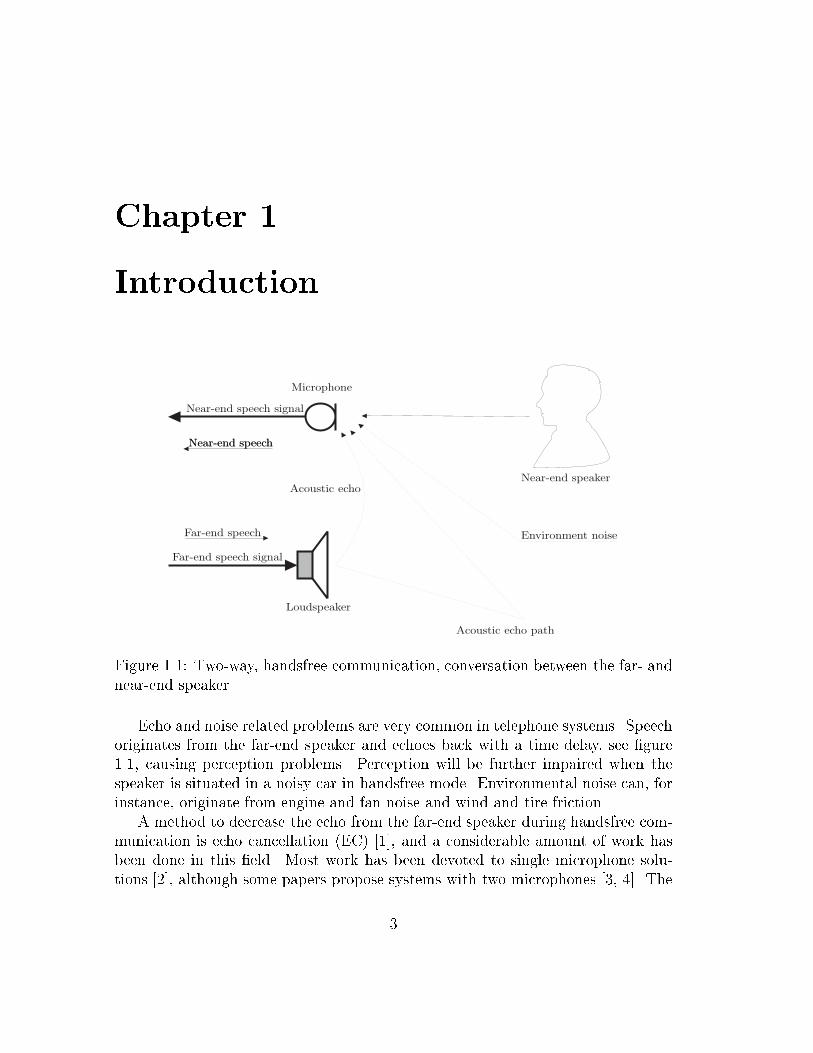
Figure 1.1: Two-way, handsfree communication, conversation between the far- and

near-end speaker.

Echo and noise related problems are very common in telephone systems. Speech

originates from the far-end speaker and echoes back with a time delay, see �gure

1.1, causing perception problems. Perception will be further impaired when the

speaker is situated in a noisy car in handsfree mode. Environmental noise can, for

instance, originate from engine and fan noise and wind and tire friction.

A method to decrease the echo from the far-end speaker during handsfree com-

munication is echo cancellation (EC) [1], and a considerable amount of work has

been done in this �eld. Most work has been devoted to single microphone solu-

tions [2], although some papers propose systems with two microphones [3, 4]. The

3

acoustic echo and noise canceller introduced in [5] is further evaluated here. The

method is not based on conventional array theory [6, 7], but relies on an indirect

calibration [8] by gathering data from the actual environment. The calibration

developed here will take on a slightly di�erent form. Di�erent adaptive algorithms

will be compared and evaluated in this report.

The system is aimed at mobile hands free communication systems, and it there-

fore should also take into account the near �eld in a small enclosure. The near �eld

is di�cult to describe in an a-priori model. This brings up the solution of employing

gathered signal-information from the real target and jammer positions. Obviously

these gathered signals contain useful information about the acoustic environment

as well as electronic equipment, such as microphones, ampli�ers, A/D-converters

and anti-aliasing �lters. Other important information is the microphone element

geometry and other spatial and spectral information inherent in the gathered tar-

get and jammer signals. Instead of calculating a large number of statistical a-priori

information from the gathered data, we will merely use the signals as they appear

during the operating phase.

The methods evaluated in this report are a Normalized Least Mean Square

(NLMS) algorithm, a fully connected Neural Network algorithm, and an optimal

Least Square solution to the normal equations where the gathered data are consid-

ered as deterministic signals, i.e. the correlations are estimated directly from the

data.

4

Chapter 2

Working Scheme for the Adaptive

Echo Canceling and Noise

Suppressing Beamformer

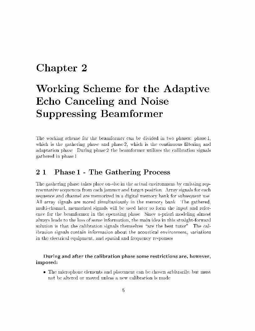
The working scheme for the beamformer can be divided in two phases: phase 1,

which is the gathering phase and phase 2, which is the continuous �ltering and

adaptation phase. During phase 2 the beamformer utilizes the calibration signals

gathered in phase 1.

2.1 Phase 1 - The Gathering Process

The gathering phase takes place on-site in the actual environment by emitting rep-

resentative sequences from each jammer and target position. Array signals for each

sequence and channel are memorized in a digital memory bank for subsequent use.

All array signals are stored simultaniously in the memory bank. The gathered,

multi-channel, memorized signals will be used later to form the input and refer-

ence for the beamformer in the operating phase. Since a-priori modeling almost

always leads to the loss of some information, the main idea in this straight-forward

solution is that the calibration signals themselves \are the best tutor". The cal-

ibration signals contain information about the acoustical environment, variations

in the electrical equipment, and spatial and frequency responses.

During and after the calibration phase some restrictions are, however,

imposed:

� The microphone elements and placement can be chosen arbitrarily, but must

not be altered or moved unless a new calibration is made.

5

x1(t)

x2(t)

xM(t)

x1 [n]

x2 [n]

xM [n]

MemoryJammercalibrationsignals

MemoryTargetcalibrationsignals

Anti-Aliasingand

A/D conversion

Figure 2.1: Target calibration signals recording.

6

x1(t)

x2(t)

xM(t)

x1 [n]

x2 [n]

xM [n]

MemoryJammercalibrationsignals

MemoryTargetcalibrationsignals

Anti-Aliasingand

A/D conversion

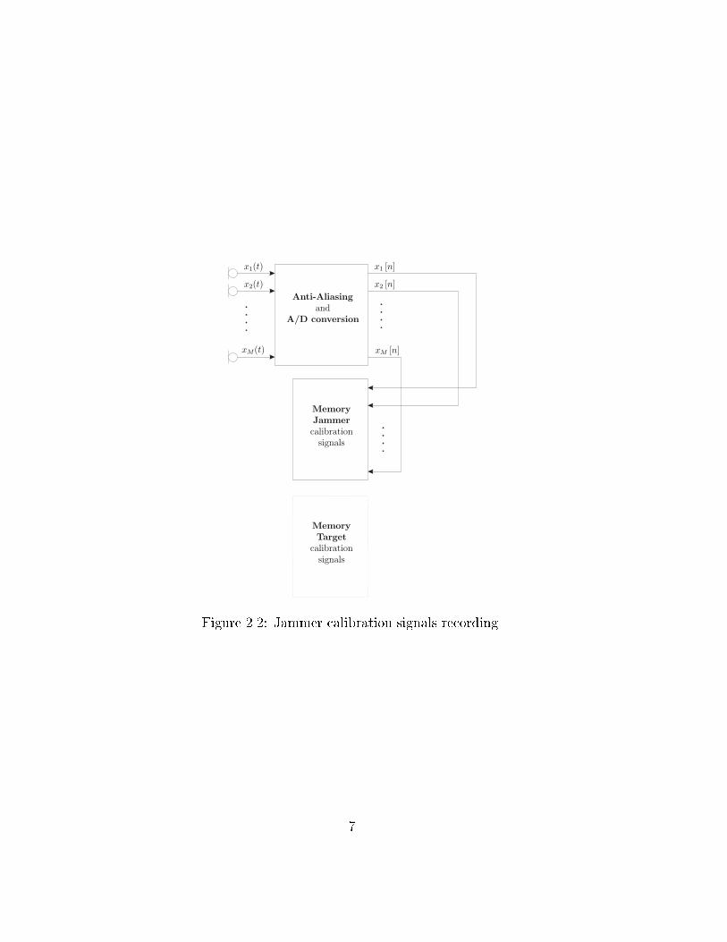
Figure 2.2: Jammer calibration signals recording.

7

� The equipment must be time invariant.

� A fair signal to noise ratio during gathering is necessary.

2.2 Calibration signals

The gathered calibration signals must arrive from the desired/unwanted (target/jammer)

positions, and the signals must contain approximately the same spectral content

as a real target/jammer signal. There are di�erent methods to facilitate these

conditions. A simple approach is to collect human utterances from the target po-

sition. A di�erent kind of calibration procedure is to place loudspeakers in the

desired/unwanted positions and let the loudspeakers emit, one at a time, at or

colored bandlimited noise, or gathered speech (see �gures 2.1 and 2.2).

2.3 Phase 2 - The Operating Mode

A telephone conversation can be divided into four modes: Idle, Receive, Transmit

and Double Talk mode.

2.3.1 Idle/I-mode

During the I-mode only car noise exists, i.e. there is no speech from the near or

far-end speaker.

Near-end speaker: quiet

Far-end speaker: quiet

Upper beamformer: Copy of LB

Lower beamformer: Adaptation on

Environmental noise impinges on each of the microphone elements in the mi-

crophone array, and is added with virtual near- and far-end speech signals, i.e. the

memorized signals. Note that the noise signals have passed through the same elec-

tronic equipment as the memorized signals. The virtually gathered speech signals

represent a speaker talking from the correct environment/position and a handsfree

loudspeaker, gathered with high SNR. These sets of signals are mixed and comprise

the inputs to the adaptive �lters (see �gure 2.3). The desired signal for the adaptive

�lters is formed by a suitable combination of the memorized target signals only.

The adaptive algorithm now has access to all the information needed to adapt the

�lters both in the spatial- and frequency-domain.

8

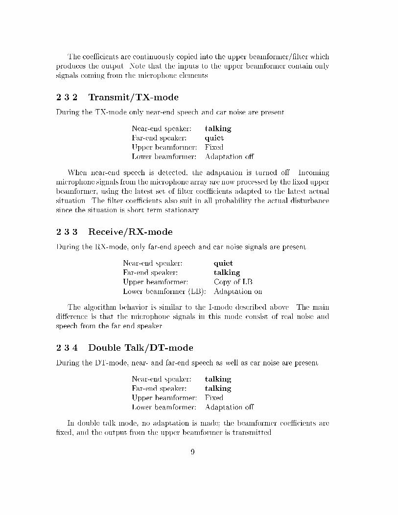
The coe�cients are continuously copied into the upper beamformer/�lter which

produces the output. Note that the inputs to the upper beamformer contain only

signals coming from the microphone elements.

2.3.2 Transmit/TX-mode

During the TX-mode only near-end speech and car noise are present.

Near-end speaker: talking

Far-end speaker: quiet

Upper beamformer: Fixed

Lower beamformer: Adaptation o�

When near-end speech is detected, the adaptation is turned o�. Incoming

microphone signals from the microphone array are now processed by the �xed upper

beamformer, using the latest set of �lter coe�cients adapted to the latest actual

situation. The �lter coe�cients also suit in all probability the actual disturbance

since the situation is short term stationary.

2.3.3 Receive/RX-mode

During the RX-mode, only far-end speech and car noise signals are present.

Near-end speaker: quiet

Far-end speaker: talking

Upper beamformer: Copy of LB

Lower beamformer (LB): Adaptation on

The algorithm behavior is similar to the I-mode described above. The main

di�erence is that the microphone signals in this mode consist of real noise and

speech from the far-end speaker.

2.3.4 Double Talk/DT-mode

During the DT-mode, near- and far-end speech as well as car noise are present.

Near-end speaker: talking

Far-end speaker: talking

Upper beamformer: Fixed

Lower beamformer: Adaptation o�

In double talk mode, no adaptation is made; the beamformer coe�cients are

�xed, and the output from the upper beamformer is transmitted.

9

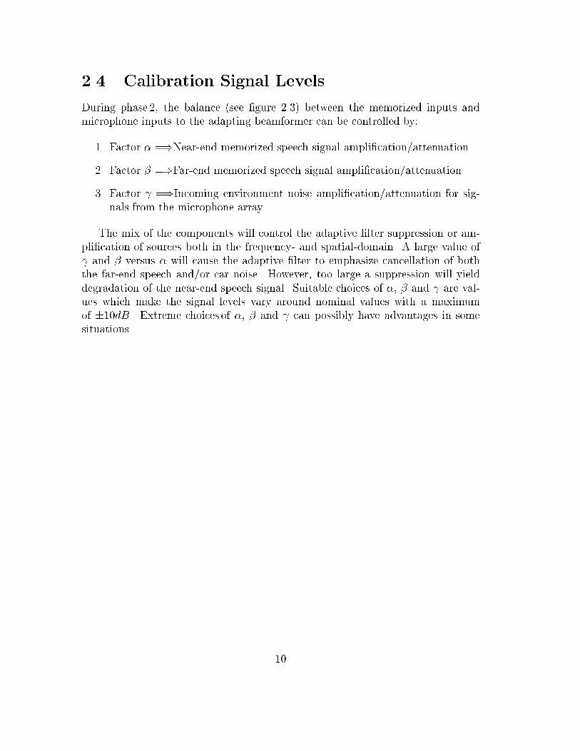
2.4 Calibration Signal Levels

During phase 2, the balance (see �gure 2.3) between the memorized inputs and

microphone inputs to the adapting beamformer can be controlled by:

1. Factor � =)Near-end memorized speech signal ampli�cation/attenuation.

2. Factor � =)Far-end memorized speech signal ampli�cation/attenuation.

3. Factor =)Incoming environment noise ampli�cation/attenuation for sig-

nals from the microphone array.

The mix of the components will control the adaptive �lter suppression or am-

pli�cation of sources both in the frequency- and spatial-domain. A large value of

and � versus � will cause the adaptive �lter to emphasize cancellation of both

the far-end speech and/or car noise. However, too large a suppression will yield

degradation of the near-end speech signal. Suitable choices of �; � and are val-

ues which make the signal levels vary around nominal values with a maximum

of �10dB. Extreme choices of �; � and can possibly have advantages in some

situations.

10

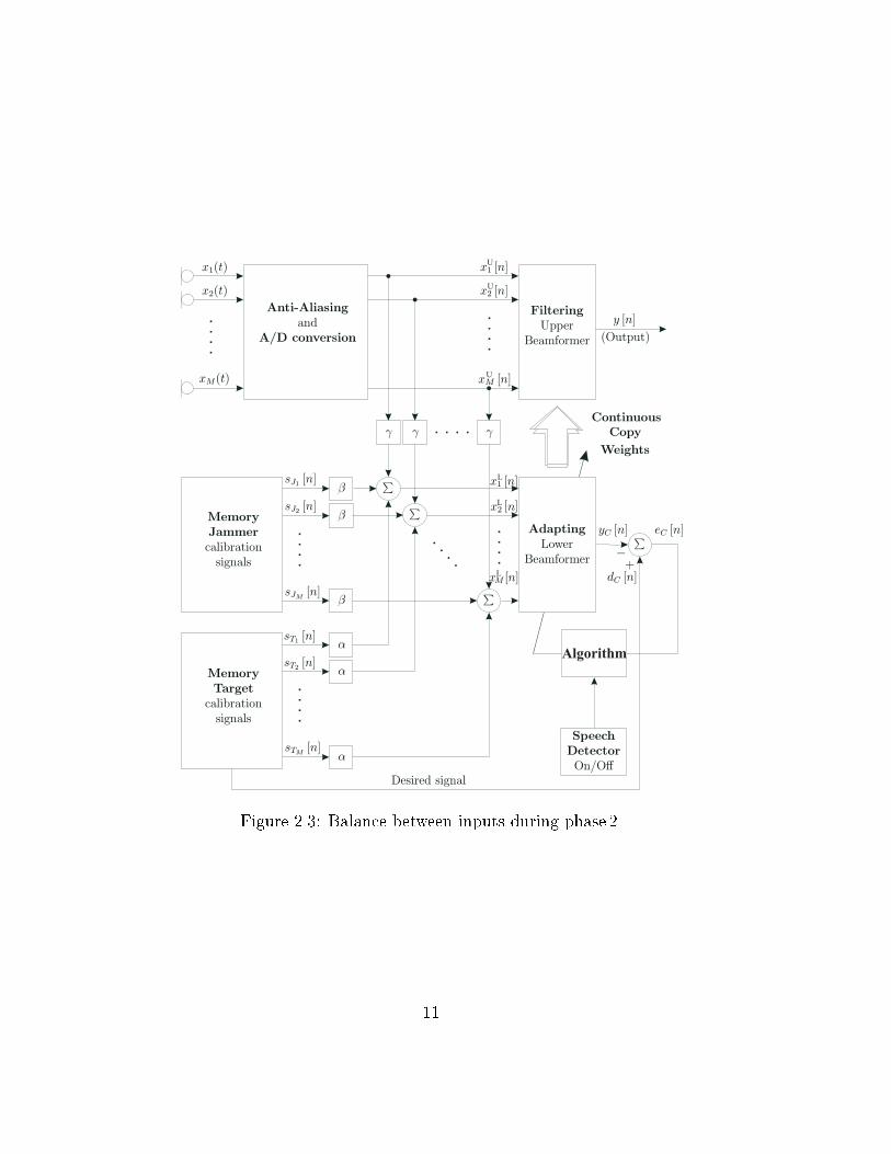
Figure 2.3: Balance between inputs during phase 2.

11

Chapter 3

Evaluation Conditions

3.1 Car Environment

The performance evaluation of the acoustic noise and echo canceling beamformer

was made in a Volvo 940 GL station wagon. Data was gathered on a multichannel

DAT-recorder with a sample rate of 12 kHz, and with a 5 kHz bandwidth. In order

to facilitate simultaneous driving and recording, a loudspeaker was mounted in the

passenger seat to simulate a real person's speaking.

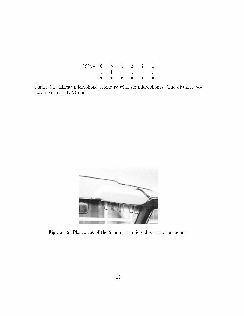
3.2 Microphone con�gurations

The microphones used in the evaluation were high quality Sennheiser microphones,

and six of them were mounted at on the visor. The distance between the speaker

position and the microphone array was 350 mm. The mounting of the linear array

can be seen in �gures 3.1 and 3.2. This con�guration were used throughout the

evaluation.

12

Mic:# 6 5 4 3 2 1

# # # # # #

� � � � � �

Figure 3.1: Linear microphone geometry with six microphones. The distance be-

tween elements is 50 mm.

Figure 3.2: Placement of the Sennheiser microphones, linear mount.

13

Chapter 4

Implementation

The data gathered from the multichannel DAT recorder was converted into Mat-

lab format, which is a conventionally used mathematics software package. The

evaluation part of the report is based on this data and all processing is done in

Matlab.

4.1 Algorithm Implementation

The lower beamformer according to �gure 2.3 has been adapted to a sequence of

band-limited noise emitted from the jammer and target positions and actual noise

in the car by making a recording of the six microphones. The resulting weights

have then been used in the upper beamformer in order to enhance the target speech

with regard to echo and noise. In the evaluation of the algorithms the parameter

L, used in the following sections, is set to 256.

4.2 Normalized Least Mean Square (NLMS) al-

gorithm

A conventional NLMS algorithm with L �lter taps for every microphone is used.

The training is done in epochs, i.e. the same training set is used iteratively. The

stepsize is normalized to the mean power of all microphone signals, furthermore the

stepsize is decreased during epochs. With FIR-�lters the output from the upper

beamformer is given by

y [n] =MXm=1

wTmx

Um [n] ; (4.1)

14

where xUm[n] denotes an L-by-1 input vector from the m-th microphone element

in the upper beamformer, and wm denotes the L-by-1 corresponding �lter weight

vector. Overscript T stands for vector transpose. The total number of �lter weights

is ML.

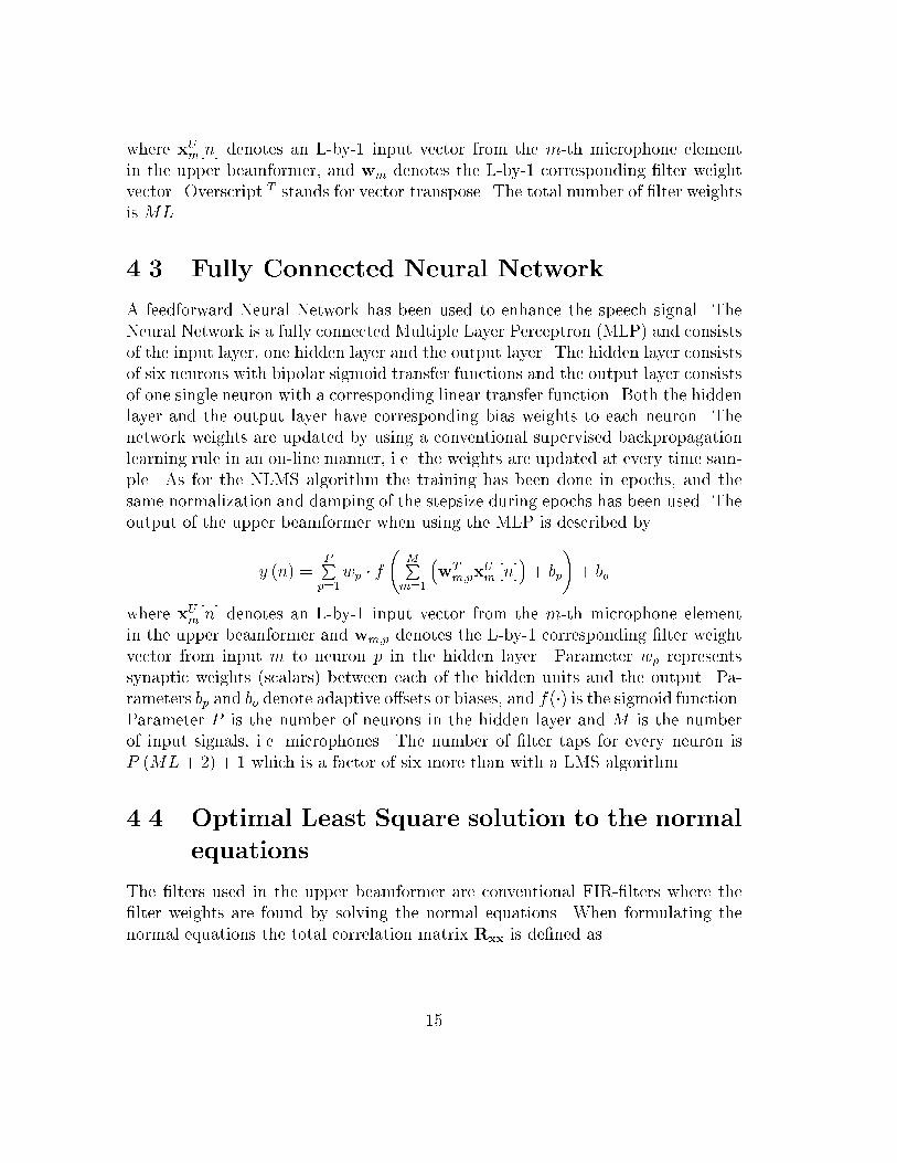
4.3 Fully Connected Neural Network

A feedforward Neural Network has been used to enhance the speech signal. The

Neural Network is a fully connected Multiple Layer Perceptron (MLP) and consists

of the input layer, one hidden layer and the output layer. The hidden layer consists

of six neurons with bipolar sigmoid transfer functions and the output layer consists

of one single neuron with a corresponding linear transfer function. Both the hidden

layer and the output layer have corresponding bias weights to each neuron. The

network weights are updated by using a conventional supervised backpropagation

learning rule in an on-line manner, i.e. the weights are updated at every time sam-

ple. As for the NLMS algorithm the training has been done in epochs, and the

same normalization and damping of the stepsize during epochs has been used. The

output of the upper beamformer when using the MLP is described by

y (n) =PPp=1

wp � f

MPm=1

�wTm;px

Um [n]

�+ bp

!+ bo

where xUm[n] denotes an L-by-1 input vector from the m-th microphone element

in the upper beamformer and wm;p denotes the L-by-1 corresponding �lter weight

vector from input m to neuron p in the hidden layer. Parameter wp represents

synaptic weights (scalars) between each of the hidden units and the output. Pa-

rameters bp and bo denote adaptive o�sets or biases, and f(�) is the sigmoid function.

Parameter P is the number of neurons in the hidden layer and M is the number

of input signals, i.e. microphones. The number of �lter taps for every neuron is

P (ML + 2) + 1 which is a factor of six more than with a LMS algorithm.

4.4 Optimal Least Square solution to the normal

equations

The �lters used in the upper beamformer are conventional FIR-�lters where the

�lter weights are found by solving the normal equations. When formulating the

normal equations the total correlation matrix Rxx is de�ned as

15

Rxx =

0BBBB@Rx1x1 Rx1x2 : : : Rx1x6

Rx2x1 Rx2x2 : : : Rx2x6...

.... . .

...

Rx6x1 Rx6x2 : : : Rx6x6

1CCCCA

where

Rxixj =

0BBBB@

rij(0) rij(1) rij(2) : : : rij(L� 1)

rij(1) rij(0) rij(1) : : : rij(L� 2)...

.... . .

......

rij(L� 1) rij(L� 2) : : : : : : rij(0)

1CCCCA

and

rij(k) =1

N

N�k�1Xn=0

xi(n)xj(n + k) ; k = 0; 1; ::::L� 1

which is a biased cross-correlation estimator due to the constant normalization

factor but gives constant varianse for all lags. This estimator is appropriate for

both deterministic and random data, so no decision regarding the form of the data

is necessary. Parameter N is the total number of time samples in the correlation

estimates. Parameter L is the number of �lter taps in the FIR-�lters.

By arranging the �lter vectors wm as a column vector

W = [wT1wT

2: : : wT

6]T

and formulating a cross-correlation vector between the desired signal d(n) and the

input signals xm(n) as

Gxd = [g1 g2 : : : g6]T

where

gi = [gi(0) gi(1) : : : gi(L� 1)]

and

gi(k) =1

N

N�k�1Xn=0

xi(n)d(n+ k) ; k = 0; 1; ::::L� 1

16

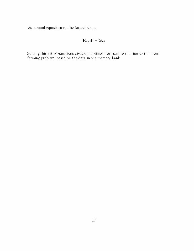
the normal equations can be formulated as

RxxW = Gxd

Solving this set of equations gives the optimal least square solution to the beam-

forming problem, based on the data in the memory bank.

17

Chapter 5

Evaluation

Performance evaluation from the Volvo is illustrated in Appendix A �gures A.1-

A.14

Common information for all plots are:

� Near-end speech, coming from the drivers seat is denoted \Speech Male/Female".

� Far-end speech echo, i.e. handsfree loudspeaker or jammer speech, is denoted

\Echo Male/Female".

� All signals are within a bandwidth of 5 kHz.

� The calibration signals are at noise within the bandwidth.

� All sequences are of 8 second duration.

� All �gures begin with 8 second sequence of the unadapted single microphone

signal from position 4, i.e. the plain un�ltered single channel microphone

signal.

� The results are presented as short time (20 ms) power estimates in dB.

In the adaptation phase (phase 2) the control parameters �; �; can be con-

trolled in order to supress or amplify the sources both in frequency and spatial

domains. The Memory-Signal-to-Interference Ratio MSIR is controlled by the

ratio between � and � by:

MSIR = 10 log

0BBB@

MPm=0

NPn=1

(� � sTm [n])2

MPm=0

NPn=1

(� � sJm[n])2

1CCCA ;

18

where sT and sJ denote the memorized calibration signals for target and jammer,

respectively. In the handsfree mode this corresponds to the speaker, usually placed

in the front seat, and the handsfree loudspeaker in the middle of the instrument

panel, directed towards the driver. The number of microphones in the array, M , is

6, while the number of samples, N , varies between 2400� 48000 in the memorized

calibration sequence.

In addition, the MSNR for the calibration phase is de�ned as:

MSNR = 10 log

0BBB@

MPm=0

NPn=1

(� � sT [n])2

MPm=0

NPn=1

( � sD[n])2

1CCCA ;

where sT and sD denote the memorized calibration signals for the target and the

actual ambient disturbances. In the car environment sD corresponds to environ-

mental car noise such as engine-, wind- and tire friction.

Keeping � �xed at 0 dB and varying � and in dB units will a�ect the MSIR

and the MSNR by the same amount.

During the �ltering phase, or the evaluation mode, the true signal level for the

jammer is used, i.e SIR = 0 dB, and for noise disturbance, SNR = �5 dB has

been used in order to make it possible to subjectively decide if any distortion is

present. This reduction does not a�ect the suppression levels in the linear cases at

all and these levels are not noticeably a�ected in the non-linear case.

The sound �les corresponding to the �gures in Appendix A, �gures A.1-A.14,

are available in .wav- format from http://www.hk-r.se/isb.

5.1 Neural Network - Performance Evaluation

The Neural Network (MLP) has been trained by using a sequence of 4800 sample

records for each input signal and the desired signal. The input signals were created

by recording an emission of band-limited at noise from the jammer and target

positions and actual noise on the six microphones in the car, while driving. The

target (desired) signals were created by doing the same recording on microphone

4 while the car was parked and the emission was done from the target position

alone, see �gure 2.3. The sequence was iterated for 1000 epochs and the stepsize

was damped exponentially from 0.1 in the �rst epoch to 0.0001 in the last epoch.

The balance parameters �, �, and were �xed at 0 dB.

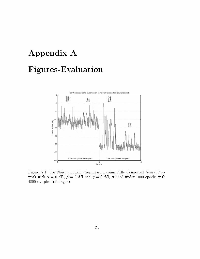
The result is shown in �gure A.1, and it can be seen that a suppression of

approximately 15 dB is achieved for both echo and noise.

19

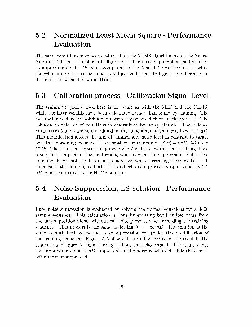
5.2 Normalized Least Mean Square - Performance

Evaluation

The same conditions have been evaluated for the NLMS algorithm as for the Neural

Network. The result is shown in �gure A.2. The noise suppression has improved

to approximately 17 dB when compared to the Neural Network solution, while

the echo suppression is the same. A subjective listener test gives no di�erences in

distortion between the two methods.

5.3 Calibration process - Calibration Signal Level

The training sequence used here is the same as with the MLP and the NLMS,

while the �lter weights have been calculated rather than found by training. The

calculation is done by solving the normal equations de�ned in chapter 4.4. The

solution to this set of equations is determined by using Matlab. The balance

parameters � and are here modi�ed by the same amount while � is �xed at 0 dB.

This modi�cation a�ects the mix of jammer and noise level in contrast to target

level in the training sequence. Three settings are compared, (�; ) = 0dB; 5dB and

10dB. The result can be seen in �gures A.3-A.5 which show that these settings have

a very little impact on the �nal result, when it comes to suppression. Subjective

listening shows that the distortion is increased when increasing these levels. In all

three cases the damping of both noise and echo is improved by approximately 1-2

dB, when compared to the NLMS solution.

5.4 Noise Suppression, LS-solution - Performance

Evaluation

Pure noise suppression is evaluated by solving the normal equations for a 4800

sample sequence. This calculation is done by emitting band-limited noise from

the target position alone, without car noise present, when recording the training

sequence. This process is the same as letting � = �1 dB. The solution is the

same as with both echo- and noise suppression except for this modi�cation of

the training sequence. Figure A.6 shows the result where echo is present in the

sequence and �gure A.7 is a �ltering without any echo present. The result shows

that approximately a 22 dB suppression of the noise is achieved while the echo is

left almost unsuppressed.

20

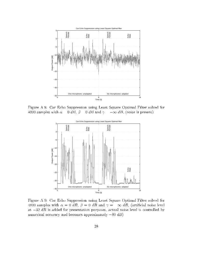
5.5 Echo Canceling, LS-solution - Performance

Evaluation

Echo canceling is evaluated in the same manner as with pure noise suppression but

with �1 dB when recording the training sequence. Figures A.8-A.9 show the

result with and without noise present (of course, some noise is always present). It

can be seen that the noise component is left almost unsuppressed while the echo

component is reduced by approximately 25 dB.

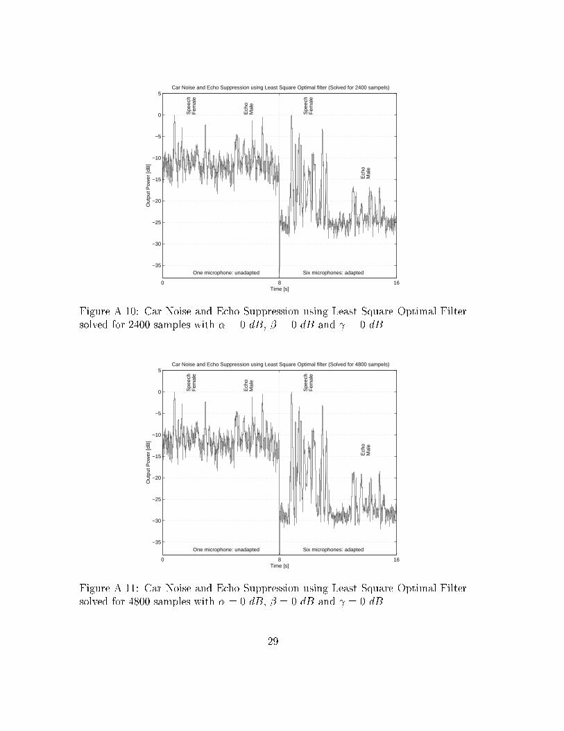
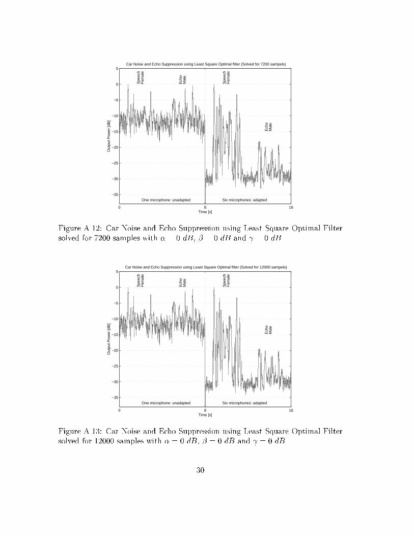
5.6 Calibration Sequence Length - Performance

Evaluation

The least square solution to both echo and noise suppression by solving the normal

equations is done here with varying length of the training sequence. The balance

parameters �, � and are held at nominal values, i.e. they are at 0 dB. Fig-

ures A.10-A.14 show the resulting suppression for di�erent selections of training

sequence length. It can be seen that increasing the training length from 12000

samples to 48000 gives only slightly better performance. The resulting suppression

with a training set of 48000 samples is approximately 20 dB for both echo and

noise. Subjective listening indicates that the distortion is small.

21

Chapter 6

Summary and Conclusions

The best resulting suppression was approximately 20 dB for both echo and noise.

This result was achieved by solving the normal equations to the beamforming prob-

lem.

The structure with non-linearities in the adaptive �lter, the Neural Network, gives

no extra performance in spite of the large number degrees of freedom, i.e. a factor

of six more weights than with the NLMS.

The scheme of training the adaptive �lter in epochs, for both NLMS and the

MLP, and by decreasing the stepsize during epochs, gives better results than by

increasing the length of the training set accordingly, compare [5]. Further, by in-

creasing the level of both � and in comparison to �, when solving the normal

equations, no extra echo and noise suppression is attained, while the distortion is

increased. The mix between echo canceling and noise suppression can be controlled

by the relative levels of disturbance, i.e. by controlling �, �, . Here, the situa-

tions of letting � and equal zero are evaluated, respectively. The result is that

when � equals zero no major echo suppression is attained, and when equals zero

no major noise reduction is attained. Approximately 25 dB echo suppression is

achieved when solving the normal equations for pure echo canceling with correla-

tion estimates based on 4800 data samples. For pure noise suppression with the

same conditions approximately 22 dB suppression is achieved.

Solving the normal equations for a 48000 sample training set gives only a slightly

better result than for a training set of 12000 samples. This indicates that further in-

creasing of the length of the training set may not increase the resulting disturbance

suppression.

22

Bibliography

[1] B.Widrow, S. D. Stearns, \Adaptive Signal Processing", Prentice Hall, 1985.

[2] M. Sondhi and W. Kellermann, \Adaptive Echo Cancellation for speech signal",

Chapter 11 in Advances in Speech Signal Processing, Edited by S. Furui and

M. Sondhi, Dekker, New York, 1992.

[3] Sen M. Kuo, Zhibing Pan, \Adaptive Acoustic Echo Cancellation Microphone",

J. Acoust. Soc. Am., vol 93, no 3,March 1993, pp 1629-1636.

[4] M. Rainer, P. Vary, \Combined acoustic echo cancellation dereverberation and

noise reduction: a two microphone approach", Ann. T�el�ecommun., 49, no. 7-8,

1994, pp 429-438.

[5] M. Dahl, I. Claesson, \Acoustic Echo Cancelling with Microphone Arrays",

Research Report 2/95, Feb. 1995.

[6] I. Claesson, S. Nordholm, \A Spatial Filtering Approach to Robust Adaptive

Beamforming", IEEE Transactions on Antennas and Propagation, vol. 40, no.

9., Sept 1992.

[7] S. Nordebo, I. Claesson, S. Nordholm, \Adaptive Beamforming: Spatial Filter

Designed Blocking Matrix", IEEE Journal of Oceanic Engineering, vol. 19, no.

4, Oct. 1994

[8] S. Nordebo, I. Claesson, S. Nordholm, B. A. Bengtsson \ `In situ' Calibrated

Adaptive Microphone Array", Research Report 2/94, ISSN 1103-1581.

23

Appendix A

Figures-Evaluation

0 8 16−35

−30

−25

−20

−15

−10

−5

0

5Car Noise and Echo Suppression using Fully Connected Neural Network

Time [s]

Out

put P

ower

[dB

]

One microphone: unadapted Six microphones: adapted

Spe

ech

Fem

ale

Ech

oM

ale

Spe

ech

Fem

ale

Ech

oM

ale

Figure A.1: Car Noise and Echo Suppression using Fully Connected Neural Net-

work with � = 0 dB, � = 0 dB and = 0 dB, trained under 1000 epochs with

4800 samples training set

24

0 8 16−35

−30

−25

−20

−15

−10

−5

0

5Car Noise and Echo Suppression using Normalized LMS

Time [s]

Out

put P

ower

[dB

]


Spe

ech

Fem

ale

Ech

oM

ale

Spe

ech

Fem

ale

Ech

oM

ale

Figure A.2: Car noise and echo Suppression using Normalized LMS algorithm with

� = 0 dB, � = 0 dB and = 0 dB, trained under 1000 epochs with 4800 samples

training set

0 8 16−35

−30

−25

−20

−15

−10

−5

0

5Car Noise and Echo Suppression using Least Square Optimal filter

Time [s]

Out

put P

ower

[dB

]


Spe

ech

Fem

ale

Ech

oM

ale

Spe

ech

Fem

ale

Ech

oM

ale

Figure A.3: Car Noise and Echo Suppression using Least Square Optimal Filter

solved for 4800 samples with � = 0 dB, � = 0 dB and = 0 dB

25

0 8 16−35

−30

−25

−20

−15

−10

−5

0


Time [s]

Out

put P

ower

[dB

]


Spe

ech

Fem

ale

Ech

oM

ale

Spe

ech

Fem

ale

Ech

oM

ale



0 8 16−35

−30

−25

−20

−15

−10

−5

0


Time [s]

Out

put P

ower

[dB

]


Spe

ech

Fem

ale

Ech

oM

ale

Spe

ech

Fem

ale

Ech

oM

ale



26

0 8 16−40

−35

−30

−25

−20

−15

−10

−5

0

5Car Noise Suppression using Least Square Optimal filter

Time [s]

Out

put P

ower

[dB

]


Spe

ech

Fem

ale

Ech

oM

ale

Spe

ech

Fem

ale

Ech

oM

ale

Figure A.6: Car Noise Suppression using Least Square Optimal Filter solved for

4800 samples with � = 0 dB, � = �1 dB and = 0 dB, (echo is present)

0 8 16−40

−35

−30

−25

−20

−15

−10

−5

0

5Car Noise Suppression using Least Square Optimal filter

Time [s]

Out

put P

ower

[dB

]


Spe

ech

Fem

ale

Spe

ech

Mal

e

Spe

ech

Fem

ale

Spe

ech

Mal

e

Figure A.7: Car Noise Suppression using Least Square Optimal Filter solved for

4800 samples with � = 0 dB, � = �1 dB and = 0 dB, (no echo present)

27

0 8 16−35

−30

−25

−20

−15

−10

−5

0

5Car Echo Suppression using Least Square Optimal filter

Time [s]

Out

put P

ower

[dB

]


Spe

ech

Fem

ale

Ech

oM

ale

Spe

ech

Fem

ale

Ech

oM

ale

Figure A.8: Car Echo Suppression using Least Square Optimal Filter solved for

4800 samples with � = 0 dB, � = 0 dB and = �1 dB, (noise is present)

0 8 16−35

−30

−25

−20

−15

−10

−5

0

5Car Echo Suppression using Least Square Optimal filter

Time [s]

Out

put P

ower

[dB

]


Spe

ech

Fem

ale

Ech

oM

ale

Spe

ech

Fem

ale

Ech

oM

ale

Figure A.9: Car Echo Suppression using Least Square Optimal Filter solved for

4800 samples with � = 0 dB, � = 0 dB and = �1 dB, (arti�cial noise level

at �32 dB is added for presentation purposes, actual noise level is controlled by

numerical accuracy and becomes approximately �80 dB)

28

0 8 16

−35

−30

−25

−20

−15

−10

−5

0

5Car Noise and Echo Suppression using Least Square Optimal filter (Solved for 2400 sampels)

Time [s]

Out

put P

ower

[dB

]


Spe

ech

Fem

ale

Ech

oM

ale

Spe

ech

Fem

ale

Ech

oM

ale



0 8 16

−35

−30

−25

−20

−15

−10

−5

0


Time [s]

Out

put P

ower

[dB

]


Spe

ech

Fem

ale

Ech

oM

ale

Spe

ech

Fem

ale

Ech

oM

ale



29

0 8 16

−35

−30

−25

−20

−15

−10

−5

0


Time [s]

Out

put P

ower

[dB

]


Spe

ech

Fem

ale

Ech

oM

ale

Spe

ech

Fem

ale

Ech

oM

ale



0 8 16

−35

−30

−25

−20

−15

−10

−5

0


Time [s]

Out

put P

ower

[dB

]


Spe

ech

Fem

ale

Ech

oM

ale

Spe

ech

Fem

ale

Ech

oM

ale



30

0 8 16

−35

−30

−25

−20

−15

−10

−5

0


Time [s]

Out

put P

ower

[dB

]


Spe

ech

Fem

ale

Ech

oM

ale

Spe

ech

Fem

ale

Ech

oM

ale



31

Acoustic Echo Cancelling and Noise Suppression with ... - DiVA

Documents

Transcript of Acoustic Echo Cancelling and Noise Suppression with ... - DiVA