Acoustic chemometrics for fluid flow quantifications - II: a small constriction will go a long way

ACOUSTIC CHEMOMETRICS FOR FLUID FLOWQUANTIFICATIONS—II: A SMALL CONSTRICTION WILL GO

A LONG WAY

KIM H. ESBENSEN1* BJØRN HOPE2, THORBJØRN T. LIED1, MATHS HALSTENSEN1, TOREGRAVERMOEN1 AND KENNETH SUNDBERG3

1Applied Chemometrics Research Group (ACRG), Telemark Technological R&D Centre (Tel-Tek) and TelemarkInstitute of Technology (HIT), Department of Process Technology (TF), Porsgrunn, Norway

2Sensorteknikk A/S, Bærum, Oslo, Norway3RAISIO Chemicals OY, Raisio, Turku, Finland

SUMMARY

A new approach for non-invasive quantitative measurement of volume flow rate, multicomponent mixtureconcentrations as well as density and other physico-chemical intensive parameters of liquid mixtures flowing inpipelines is presented, based on novel application extensions of the well-known orifice plate principle(extensively used for flow measurement in pipes). By deliberately transgressing the conventional usage limits,the orifice plate configuration may now also be used for a range of new measurement types, all based on acousticsensor technology. R&D has been carried out since 1987 by Sensorteknikk A/S and since 1994 in collaborationwith ACRG.

The acoustic chemometricsconcept is characterized by easy ‘clamp-on’ deployment of acoustic sensors(primarily accelerometers), followed by an essential, integrated signal analysis/multivariate calibration datamodelling, well known from chemometrics. The signal analysis step in this endeavour is often critical althoughrarely outside conventional electrical engineering scopes. We present three fluid/fluid or fluid/solid mixtureapplication type cases: (1)trace oil-in-water determination (representingone-analyte systems); (2) jet-fuel/glycol mixture determination (representingtwo-analyte systems); (3) paper-pulp constituent(s) determination(representinganalyte–interferents systems). We also describe extension studies of these first quantitative acousticchemometrics forays, e.g. for alternative measurement of (conventional) flow velocities of both fluid/fluid andfluid/solid (slurries) systems (average volume flow rate of heterogeneous multiphase systems), for flow regimecharacterization and for measurement of the effective in-line density of (fluid/fluid and fluid/solid) mixtures.There would appear to be a vast potential for technological and industrial applications of this new type ofacoustic chemometric process and product characterization/monitoring. Copyright 1999 John Wiley & Sons,Ltd.

KEY WORDS: acoustic sensor technology; acoustic chemometrics; orifice plate extensions;chemometrics; multivariate calibration; analyte predictions; measurement technology;industrial applications

JOURNAL OF CHEMOMETRICSJ. Chemometrics13, 209–236 (1999)

* Correspondence to: K. H. Esbensen, ACRG, Telemark Institute of Technology, Department of Process Technology,Porsgrunn, Norway.Contract/grant sponsor: HIT-TF.Contract/grant sponsor: Royal Norwegian Research Council.Contract/grant sponsor: Tel-Tek.Contract/grant sponsor: BRITE-EURAM III.

CCC 0886–9383/99/030209–28 $17.50Copyright 1999 John Wiley & Sons, Ltd.

Received 22 September 1998Accepted 1 March 1999

INTRODUCTION: DIFFERENTIAL FLOWMETERS AND BEYOND

Quantitative measurement of flow rates of materials through pipelines is of paramount importance ina wide range of technological and industrial settings. This includes—but is in no way limited to—chemical industries, the oil and gas industry, the mineral, steel and food industries (in general,process industries) and is no less important in public utility sectors (e.g. waste treatment) as well as inenvironmental technologies etc. There are available a large and bewildering number of types offlowmeters for point measurements, volume measurements (volume flow rate), mass flow rate etc.,and the problem of choosing the right instrumentation for any specific application is not trivial. Thearea of ‘principles of measurement systems’ constitutes a basic prerequisite for very many complexengineering endeavours, and there are consequently a score of modern, well-reputed textbooks in thisarea. Suffice here to refer to only one, which may serve as a general reference in this context, theeminent textbook of Bentley.1

Fluid flow in enclosed tracts in general and internal fluid flow in regular cross-sectioned pipelinesin particular have received an almost unlimited R&D interest throughout all of the history of theengineering sciences—for very obvious technological reasons. In this paper we do not pretend toaddress all of this immense area; we of course have to restrict ourselves—the following curtails theefforts and results reported in this paper.

. Circular-sectioned, straight pipelines of ‘medium dimensions’ (diameters in the cm–dm range).

. Pipeline materials: conventional (cast-iron, copper, steel, alloys), i.e. all results reported herepertain to metal inner pipeline wall materials—which is important w.r.t. the kind of flowregimens that can be realized (laminar; transitional, turbulent flow regimens), especially in the(near-wall) boundary regions. So far we have investigated systems with a Reynold’s numberRetypically>104, corresponding to fully developed turbulent flow conditions at the position of ouracoustic chemometric recordings.

. Only liquid states are covered in this report. Liquidsflow when subjected to shear stresses,likewise low-viscosity solid/fluid mixtures (suspensions, dilute slurries); see Reference 2 forgas/solid systems.

. Only incompressible materials have been investigated, i.e. it is assumed that the type ofcompression experienced in the orifice plate measurement configurations used here does not leadto any significant changes in the density of the materials being characterized.

Fromfluid dynamicsthe most important conservation principle for the present applications is thetotal energy conservation for an incompressible fluid, which for horizontal, straight pipelines reducesto thevolume flow rate conservationprinciple

A1v1d1 � A2v2d2 �1�

where A is the cross-sectional area,v is the velocity andd is the density at locations 1 and 2respectively. Ford1 = d2, equation (1) is themass flow rate conservationlaw.

Bentley1 (Chap. 12) develops the pertinent theoretical descriptions of the archetypal D/P(differential pressure) volume flowmeters, the Venturi tube and the orifice plate (Figure 1), the twoby-far most common volume flowmeters in use. A first description of the common principle for bothtypes is simple—aconstrictionis placed in the pipeline, reducing the effective inner cross-sectionalarea of the conduit. This extremely simplistic interaction with the flowing medium results in a quiterefined measurement possibility opening up however, based on the fact that a significant differentialpressure drop is developed across the constricting element. For the sudden constriction of the orificeplate, for example, the cross-sectional area (� D2/4, whereD is the pipe diameter) is typically

210 K. H. ESBENSENET AL.

Copyright 1999 John Wiley & Sons, Ltd. J. Chemometrics, 13, 209–236 (1999)

forcefully reduced to about 0⋅6 (�d2/4, whered is the flowmeter inner diameter) at the plane of the so-calledvena contracta1 (see also further dicussions below). Both the Venturi tube and the orifice platedevices make use of the resulting pressure differential across the flow constriction. The technicalmeasurement problem is simply how to infer the volume flow rate accurately enough from themeasured differential pressures at two pressure tappings.

In reality, however, this quantitative calibration between the differential pressure and thecorresponding volume flow rate is anything but simple. This is an intrinsically non-linear relationship,although usually tractable; much worse: proper localization of the most optimal set of pressure-measuring tappings is almost an ‘art’. It has also been found necessary to introduce at least twoempirical corrections factors—C, the discharge coefficient, andE, the velocity-of-approach factor—in order to arrive at a practical D/P–v equation.1 Not only that, but these correction factors both havecomplex, partly interrelated dependences on the type of flowmeter used, the flow regimen, theReynolds number, etc. In general, extensive empirical technical tables or calibrated computersoftware have to be used in individual cases. The complete command of differential pressureflowmetering is no small feat, but a rather intricate technological challenge for any new generation ofengineering students. Still—as is evident in the non-disputed, successful widespread use of suchdevices—differential pressure flowmeters are by far the most often used techniques for volume(mass) flow rate quantification, but with some (very) notable provisos.

1. The inner piping walls must be as smooth as possible, lest significant interfering boundary layercomplications arise; these are of course primarily related to the friction along the inner walls.The assumption of frictionless flow actually does not hold up completely in reality, but for themore successful D/P flowmeters a reasonable near-zero andconstantfriction realization wouldappear not to hamper their actual use, and in many practical cases it is meaningful to speak of anaverage velocity across the cross-section of the pipeline.

2. There isalwayssome permanent pressure loss (�PP) across a constrictive flow obstructionowing to these frictional effects, either along the inner walls and/or due to inner friction effectsin the liquid itself. Internal friction is also pronounced for flowing multiphase mixtures (solid/fluid and gas/liquid mixtures). The pressure drop may result in extra pumping energy beingneeded (the extra costs may even be economically significant for large installations). Thispermanent pressure loss for the orifice plate is relatively severe compared with other principlessuch as the Venturi and the Dall tube, but the orifice plate’s simplicity and its consequent veryinexpensive general costs often still make it preferable (it is e.g. available in absolutely ‘any

Figure 1. Two most used differential pressure (D/P) flowmeter principles, based on flow constriction. Left:designedflow constriction—the Venturi tube. Right:forcedconstriction—the orifice plate. Note back-circulationcells andvena contractafor the orifice plate. Also note disposition of the essential pressure tappings for

measuring the pressure differential

ACOUSTIC CHEMOMETRICS—II 211


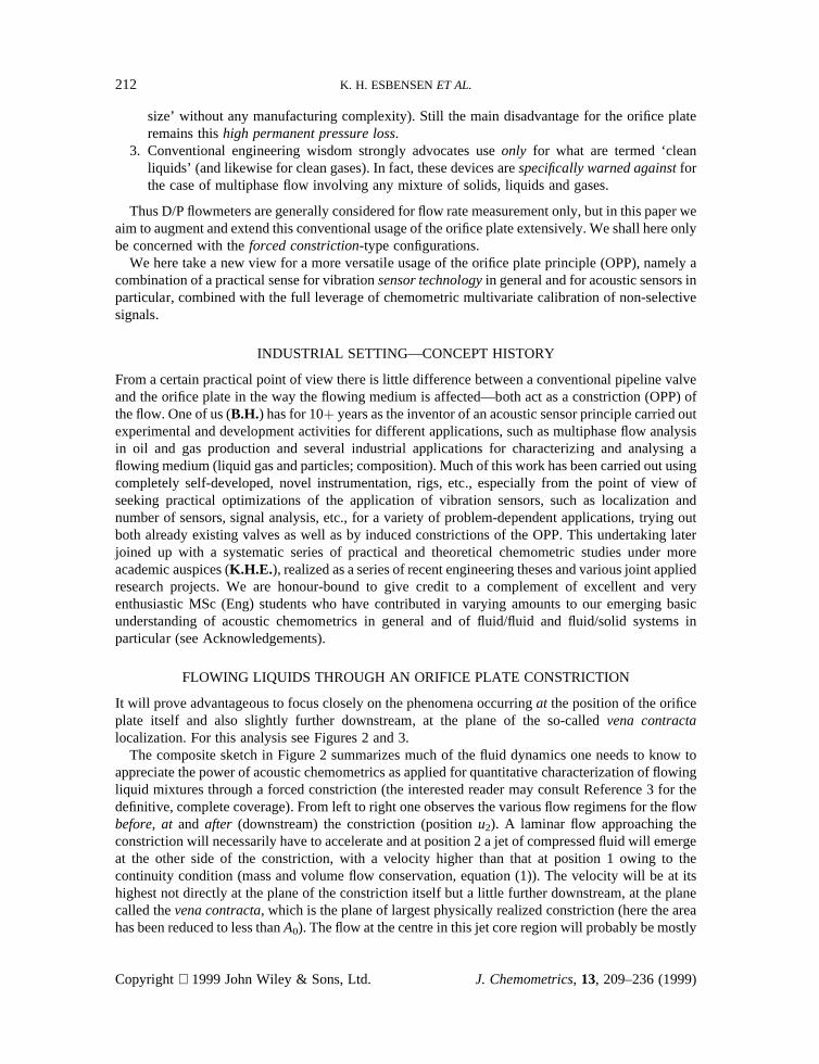
size’ without any manufacturing complexity). Still the main disadvantage for the orifice plateremains thishigh permanent pressure loss.

3. Conventional engineering wisdom strongly advocates useonly for what are termed ‘cleanliquids’ (and likewise for clean gases). In fact, these devices arespecifically warned againstforthe case of multiphase flow involving any mixture of solids, liquids and gases.

Thus D/P flowmeters are generally considered for flow rate measurement only, but in this paper weaim to augment and extend this conventional usage of the orifice plate extensively. We shall here onlybe concerned with theforced constriction-type configurations.

We here take a new view for a more versatile usage of the orifice plate principle (OPP), namely acombination of a practical sense for vibrationsensor technologyin general and for acoustic sensors inparticular, combined with the full leverage of chemometric multivariate calibration of non-selectivesignals.

INDUSTRIAL SETTING—CONCEPT HISTORY

From a certain practical point of view there is little difference between a conventional pipeline valveand the orifice plate in the way the flowing medium is affected—both act as a constriction (OPP) ofthe flow. One of us (B.H.) has for 10� years as the inventor of an acoustic sensor principle carried outexperimental and development activities for different applications, such as multiphase flow analysisin oil and gas production and several industrial applications for characterizing and analysing aflowing medium (liquid gas and particles; composition). Much of this work has been carried out usingcompletely self-developed, novel instrumentation, rigs, etc., especially from the point of view ofseeking practical optimizations of the application of vibration sensors, such as localization andnumber of sensors, signal analysis, etc., for a variety of problem-dependent applications, trying outboth already existing valves as well as by induced constrictions of the OPP. This undertaking laterjoined up with a systematic series of practical and theoretical chemometric studies under moreacademic auspices (K.H.E.), realized as a series of recent engineering theses and various joint appliedresearch projects. We are honour-bound to give credit to a complement of excellent and veryenthusiastic MSc (Eng) students who have contributed in varying amounts to our emerging basicunderstanding of acoustic chemometrics in general and of fluid/fluid and fluid/solid systems inparticular (see Acknowledgements).

FLOWING LIQUIDS THROUGH AN ORIFICE PLATE CONSTRICTION

It will prove advantageous to focus closely on the phenomena occurringat the position of the orificeplate itself and also slightly further downstream, at the plane of the so-calledvena contractalocalization. For this analysis see Figures 2 and 3.

The composite sketch in Figure 2 summarizes much of the fluid dynamics one needs to know toappreciate the power of acoustic chemometrics as applied for quantitative characterization of flowingliquid mixtures through a forced constriction (the interested reader may consult Reference 3 for thedefinitive, complete coverage). From left to right one observes the various flow regimens for the flowbefore, atand after (downstream) the constriction (positionu2). A laminar flow approaching theconstriction will necessarily have to accelerate and at position 2 a jet of compressed fluid will emergeat the other side of the constriction, with a velocity higher than that at position 1 owing to thecontinuity condition (mass and volume flow conservation, equation (1)). The velocity will be at itshighest not directly at the plane of the constriction itself but a little further downstream, at the planecalled thevena contracta, which is the plane of largest physically realized constriction (here the areahas been reduced to less thanA0). The flow at the centre in this jet core region will probably be mostly



laminar. Exactly where turbulence sets in is a matter for ongoing research, as theoretical derivationsinvariably do not express an exact fit with reality,3 but downstream the jet configuration will veryquickly break down completely and a regimen of turbulent flow will develop (between localizationsu2 andu3), also due to interaction with the characteristicbackcirculation cellswhich are developed inthe areas near the pipeline walls close to the constriction. In region 3 a fully developed turbulent flowwill always be present for all the currently interesting approach velocities (i.e. we are not concernedwith downstream laminar flow situations/applications). The term ‘turbulent flow’ needs to becarefully defined: ‘Motion of an irregular flow condition in which the various quantities show arandom variation with the time and space co-ordinates, but so that statistically significant averagevalues can be discerned’.4 An alternative view is: ‘Turbulence is an irregular eddying motion in

Figure 2. Schematic overview of turbulence phenomena developing downstream of orifice plate flowconstriction; see text for details. In the bottom part are depicted the cross-sectional velocity distributions at fourlocationsbeforeandat the orifice plate itself, as well as in thearea offully developedturbulence(u3), in whichthe random or chaotic velocity distribution is evident. Further downstream (u4) the flow gradually reverts to its

pre-orifice plate laminar flow regimen (transitional regimen)



which velocity and pressure pertubations occur about their mean values; these pertubations areirregular or random, even chaotic, in time and space, with components extending smoothly over anextensive continuous hierarchy of scales or frequencies so that they must be characterized bystatistical means’.5

Across the constriction the static pressure drops severely at position 2—the Bernoulli effectexplains that as the kinetic pressure goes up as the flow passes through the constriction, the potentialenergy (the static pressure) necessarily must go down here where the flow is manifested by high(er)velocities. The sum of the static and the dynamic pressure isnot constant over the constrictionhowever, as a differential pressure drop across the constriction will be produced (� PP). This is amanifestation of an energy loss associated with the turbulent flow regimen—this energy loss willmainly show up asvibrational energy in the total system (orifice plate/pipeline walls/flowingmedium) and will partly also show up as heat loss. Figure 2 shows clearly how the sum of the staticand the dynamic pressure drops across the constriction. This pressure differential can also be seen asrepresenting a new, potential information source for another type of flowing medium quantification—and which, as shall be amply demonstrated below, is much more information-rich than merely withrespect to the average flow rate as in the conventional D/P flowmeters.

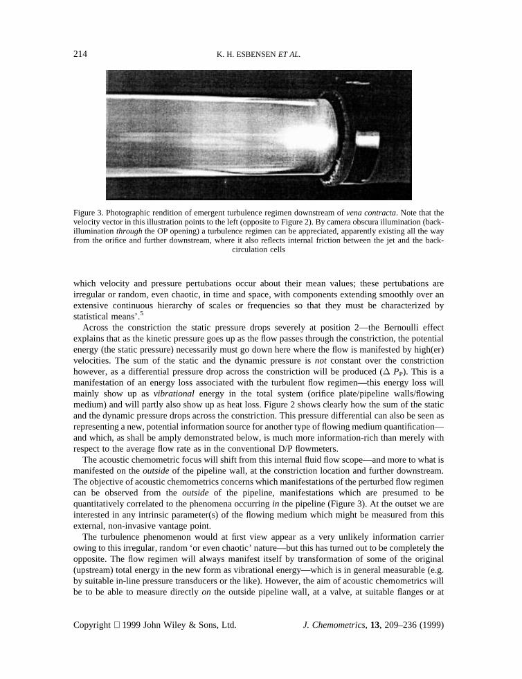
The acoustic chemometric focus will shift from this internal fluid flow scope—and more to what ismanifested on theoutsideof the pipeline wall, at the constriction location and further downstream.The objective of acoustic chemometrics concerns which manifestations of the perturbed flow regimencan be observed from theoutside of the pipeline, manifestations which are presumed to bequantitatively correlated to the phenomena occurringin the pipeline (Figure 3). At the outset we areinterested in any intrinsic parameter(s) of the flowing medium which might be measured from thisexternal, non-invasive vantage point.

The turbulence phenomenon would at first view appear as a very unlikely information carrierowing to this irregular, random ‘or even chaotic’ nature—but this has turned out to be completely theopposite. The flow regimen will always manifest itself by transformation of some of the original(upstream) total energy in the new form as vibrational energy—which is in general measurable (e.g.by suitable in-line pressure transducers or the like). However, the aim of acoustic chemometrics willbe to be able to measure directlyon the outside pipeline wall, at a valve, at suitable flanges or at

Figure 3. Photographic rendition of emergent turbulence regimen downstream ofvena contracta. Note that thevelocity vector in this illustration points to the left (opposite to Figure 2). By camera obscura illumination (back-illumination throughthe OP opening) a turbulence regimen can be appreciated, apparently existing all the wayfrom the orifice and further downstream, where it also reflects internal friction between the jet and the back-

circulation cells



similar external constricting construction details. Such measurements need not necessarily besimple—indeed, one would expect quite the opposite because of the very nature of the inherentlycomplex turbulence phenomenon. As it will transpire, however, a combination of modern vibrationsensor technology, conventional engineering signal analysis and chemometric multivariatecalibration is quite up to the job.

ACOUSTIC CHEMOMETRICS (AC)

The development of the downstream flow regimen—for the present theoretical point of view—can beconsidered as dependent upon (amongst other factors) the upstream approach velocity of the flowingmedium, the contrast between the pipeline diameter (D) and the constriction hole diameter (d), i.e.,D/d, the the physical form of the orifice opening, the temperature and viscocity of the flowing mediumas well as the composition of the flowing mixture(s). The aim for acoustic chemometrics will be toaddress, in principle, all these factors. A more fully developed concept ofacoustic chemometricscanbe expressed in the following compact form.

The ‘constriction’ acoustic chemometric approach makes use of sensor-specific domaintransformations of one or more acoustic sensor signals characterizing avibration spectrum of aturbulence regimendeveloped downstream of a pipeline constriction (designed or forced), asX-inputfor a chemometric multivariate calibration of parametersY related to the flowing liquid medium, e.g.flow velocity, analyte/mixture concentration(s), density, temperature or other physical or colloidalcharacteristics.

The main features of a parallel development track of ‘non-constricting’ acoustic chemometrics

Figure 4. (a) Generic data path flow sheet in acoustic chemometrics; see text for details. (b) Example of resultingraw FFT spectrum obtained, used asX-data in PLS-R.X-variables (nos 0–250) onX-axis reflect the frequencyrange 0–25 kHz. The two spectra shown correspond to oil concentrations of 11 and 27 ppm (see Figure 10)



were recently also laid out in a companion paper;2 these two papers complement each other, but mayof course be read independently.

INSTRUMENTATION

The acoustic chemometric data path principally includes four main elements.

1. Sensor technology: type/number of sensor(s); mounting; positioning; etc.2. Data acquisition: cabling; signal conditioning; amplification; filtering; A/D conversion.6

3. Signal analysis/domain transformation:7 FFT, AMT (angle measure technique),6 wavelets ofthe X-data (standard regression terminology).

4. Multivariate calibration w.r.t. the parameter(s) of interest (Y-variables). Figure 4(a) is aschematic flow sheet showing ageneric data pathfrom the acoustic phenomenon to the finalmultivariate calibration model, including future prediction facilities.

The main types of acoustic sensors include a suite of generic accelerometers (usually standardindustrial units are quite sufficient) as well as more specialized units (proprietary). Both portablerecorders as well as desktop or lab-bench PC-based data I/O links are in widespread use. Wheneverpossible the use of direct PC-based data acquisition boards is preferable,7 but pilot studies in the field,frequently taking place under severely non-optimal conditions, often necessitate rugged and durablesolutions, DAT recorders, etc.

All HW solutions are backed by the powerful LabVIEW SW system (National Instruments Inc.),8

allowing for problem-dependent construction of dedicated virtual instruments. LabVIEW is used tocontrol the necessary signal conditioning and the final data acquisition—often also to calculatestandard on-line domain transformations such as the fast Fourier transform (FFT). Forethought andexperience are often needed in the estimation of the relevant domain transformation to achieve anoptimal frequency representation of the time domain signals (Figure 4(b) ).

The success of many sophisticated multivariate measurement techniques (e.g. in spectroscopy) isin no small measure due to application of the versatile multivariate PLS regression approach. Owingto thenon-selectivenature of types of multivariate instruments, chemometrics is often indispensableand becomes an integral part of such measurement concepts. Although chemometrics originates fromchemistry, it is now also a generic discipline of much more general data analytical applicationpotential. In the present context the combination of applied engineering, signal analysis, electronicsand chemometrics forms a particularly strong example of a new interdisciplinary foray into acompletely virgin territory—acoustic chemometric monitoring and control of industrial, laboratoryand scientific processes attended by a suitable ‘noise output’. As we aim to demonstrate the potentialappears to be large indeed.

EXPERIMENTAL DESIGNS IN AC METHODOLOGY DEVELOPMENT

With the use of systematicexperimental designit is possible to gain much quantitative informationeven at a low experimental effort. In chemometrics, usually one form or other of traditionalorthogonal designs (e.g. full or reduced factorial design) is used initially in order to pinpoint which(major and interaction) factors display a significant effect on the response, i.e. screening designs. Forfollow-up work there is a wide variety of subsequent optimization designs.9 The random designconcept is a flexible and efficient alternative design method2 which can be used for both screening andoptimization purposes when dealing with complex systems—a useful alternative e.g. when there aremany variables and levels to be investigated and/or when the desired number of levels for eachvariable is different. The random design is phenomenologically closely related to the type of optimalspace-filling designs, although the total number of runs can be more relaxed.



The central tenet is to use uncoded design variables and to randomly select levels for each factor orvariable from within appropriately specified minimum and maximum limits—and to interpretresponse relationships using a standard PLS regression. With this approach the experimental factorsare assured a maximum degree of interaction (correlation) support as well as a quite satisfactory near-optimal spread in the (X,Y)-variance directions. The random design has been found useful forregression modelling of many of our kind of complex technological systems, as it is sure to span theentire set of ranges in the operating domain, especially as concerns interactions. This also results in asatisfactory range covering in theY-domain (see, e.g. Figure 14). The random design approach allowsfor the full PLS advantage of using the appropriately validated optimal number of components—inopposition to the so-called fully orthogonal designs in which only one PLS component is needed.With the random design one is free to choose practically any number of experiments to be carriedout—often just a fraction more experiments than the traditional absolute minimum for a comparablescreening design, typically a total of less than some 25% more runs. This is the price to pay in orderalso to be able to go directly from initial experimentation to the final PLS regression evaluation. In thepresent context we have been able to obtain very useful information with a typical number of runs ofthe order of 20–30 or less. All initial AC implementation/recording optimization (see below) wasmostly based on traditional screening designs, while most subsequent application runs for the mostpart were based on the random design approach.

Very many basic investigations have been carried out in order to facilitate a general basis forestablishing accurate and representative AC recording/data acquisition/signal analysis optimizations,e.g. regarding accelerometer/amplification/filtering responses, etc. It is of course imperative toacquire acoustic signals with the highest possible quality, and this is affected by signal conditioningoptimization, etc., grounding, gain setting, optimal filter cut-off frequencies as well as by problem-dependent amplification gain settings. In order to optimize practicalPSD (power spectral density)estimation of the signal by means of its fast Fourier Transformation (FFT), the number ofperiodograms (temporaryPSD) used to produce representative averagePSDsand the number ofsamples used to compute each periodogram are two essential parameters, which were also subjectedto experimental design optimization for individual measurement contexts. The use of a frame size of4096 together with 75 averages proved to be useful to average data acquisition parameters over manyof our typical stationary acoustic signals. Concern also has to be taken when estimating thePSDsinorder to preserve the information and minimize ‘spectral leakage’.10 There is no particular need to goany further into FFT theory for the present practical purposes; if necessary, the complete backgroundcan easily be located.10

DATA MODELLING: PLS REGRESSION

The AC regression models are to be developed through multivariate calibration (PLS-R). Thesemodels describe the relationship between the acousticX-spectra and the measuredY-characteristics ofinterest and are typically to be used for future real-time predictions of the pertinentY-parameter(s)—perhaps to serve in an on-line MSPC context or the like. In this paper we are exclusively concernedwith process/product monitoring possibilities though.

Multivariate calibration in general is dealing with the two matricesX and Y, containing theindependent input variables (X) and the dependent response or output variables (Y). The inputvariables may well be correlated (which is certainly the case here with thePSDspectra) and thereforenot suited for standard ML regression analysis. Partial least squares regression (PLS-R) handles thissituation with conviction (see literature below). It is of course of critical importance that the (X,Y)-data containrelevant prediction informationfor the relationships to be modelled, which in the presentcase has been verified abundantly by a score of AC studies in our laboratory. Descriptions of the two



most frequently used methods, principal component analysis (PCA) and partial least squaresregression (PLS-R), need not be given here; details can be found in References 11–14.

The two multivariate calibration matrices in the present experimental context contain the FFTspectra in theX-block (PSD spectra), while theY-vector(s) correspond to the particular parameter(s)of interest. The presentX-data contain the optimally recorded, relevantly signal-analysed (Fourier-transformed) acoustic spectra, characterizing a well-spanning set of operating conditionsrepresentative for technological and industrial process/product characterization, to be calibratedagainst the relevantY-vector(s).

All PLS modelling in this paper exclusively used the UNSCRAMBLER.15

ACOUSTIC CHEMOMETRIC OPP TO QUANTIFY MULTIPHASE/MULTICOMPONENTSYSTEMS

Acoustic chemometric OPP is now to be used for multicomponent or multiphase mixture systemswhich display enough essential similarities to the fluid dynamically ‘clean liquids’ detailed above thatsimilar flow regimens through the constricting element(s) will result. In other words, AC wants tomake use of the OPP in an exploratory, empirical sense by simply trying out this new, externalmeasurement principle in practice—in the laboratory as well as in pilot industrial and technologicalapplication settings. Our current AC drive has been carried out as a closely knitted two-track, parallelendeavour, with basic investigations in the laboratory and concomitant trials in real-world plantsettings.

It was early on decided to build an experimental rig (see Figure 5) on which to carry out basicresearch on the physics of AC specifically restricted to thenon-cavitating regimen;all results

Figure 5. Schematic outline of experimental HITAFF rig on which most studies reported here have been carriedout. The rig allows realistic flow conditions to be studied at ‘Measurement zone 1 or 2’ (this paper). Allexperimental mixing of fluid/solid components takes place both in the tank as well as through the necessary

number of fill rig/tank passages to reach homogeneity



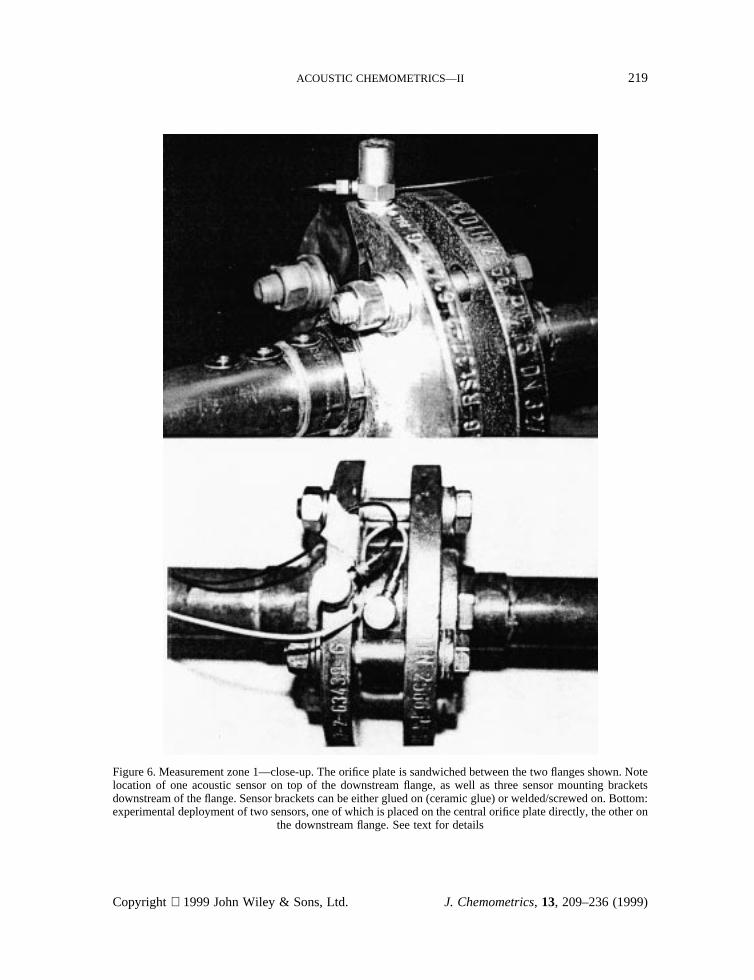
Figure 6. Measurement zone 1—close-up. The orifice plate is sandwiched between the two flanges shown. Notelocation of one acoustic sensor on top of the downstream flange, as well as three sensor mounting bracketsdownstream of the flange. Sensor brackets can be either glued on (ceramic glue) or welded/screwed on. Bottom:experimental deployment of two sensors, one of which is placed on the central orifice plate directly, the other on

the downstream flange. See text for details



presented here exclusively pertain to this flow regimen. (It should be noted that a larger, pilot plant-scale, experimental rig for multiphase investigations also in the cavitating regimen resides atSensorteknikk A/S.)

THE HITAFF EXPERIMENTAL RIG—OPTIMIZATION OF AC MEASUREMENTTECHNOLOGY

Figure 5 shows a schematic overview of the layout of the non-cavitating HITAFF experimental rig. Apositive displacement pumping unit ensures a reasonable pumping capacity, which translates intorealizable approach velocities in the interval 0–3 m s71, with a continuous variable actuator—thusany velocity in this interval is easily attainable for the experimentalist. The rig is equipped with amixing tank in which almost any compositional fluid mixture can be prepared with comparable ease;the tank plus rig volume totals some 130 l. Great care is always needed to ensure effective, completemixing, at best already in the tank, but it is of course also useful to have the entire volume circulatinga sufficient number of times through the rig before commencing actual AC experiments (‘wetting’ thesystem).

Figure 6 shows details of the singular most important part of the rig, the experimental ACmeasurement zone, in which a wide array of orifice plates, valves, etc. can be fitted. It shows e.g.details of an orifice plate sandwiched between two mounting flanges, which allows for speedysubstitution of OP inserts (e.g. with differentvena contractadiameters, etc.). Figure 6 showsexamples of some of the extensive series of sensor localizations which have been carried out in thissetting—amongst other things, sensor localizations both on the OP itself and on the downstreamflange, as well as on the pipeline wall at various downstream distances from the constriction.

With this general framework a large series of systematic studies have been carried out during the

Figure 7. Final optimized acoustic chemometric orifice plate/sensor configuration. Optimal sensor locationcorresponds to A applied directly on the OP (either glued on or welded on); locations B and C are suboptimal for

most situations



last 3–4 years. Focus has been on the following influencing factors:

(i) approach velocity(ii) sensor location(iii) number of sensors (one to four sensors)(iv) type of sensor(v) OP constriction opening diameter (also alternative opening geometries, e.g. cone shape)(vi) fluid mixture composition(vii) type of mounting of sensor (bracket, welded-on, glued-on, screwed-in)(viii) temperature (constant or varying—will vary in industrial applications).

There are actually even more potential experimental factors than these eight, which on occasionalso have been invoked, but this list suffices to illustrate that the way to go about experimenting withAC in this setting needs a solid understanding of the concepts and a good practical knowledge ofproper experimental design. All standard statistical designs used in these works are based on theprogram MODDE, version 4⋅0 from Umetrics.16 Clearly, full seven- or eight-factor designs are notpractically realizable given this rig and its construction, but extensive use has been made of selectedfractional factorial designs for the many forays into the matters of optimizing the recordingparameters of acoustic chemometrics as defined above, in order to keep the total experimental work—even with a healthy supply of MSc students—at a reasonable level. More recent work has specificallyconcentrated on investigating the effects of the supposed major factors: approach velocity,D/d (forconstantD the constriction diameterd is varied), constriction cross-section geometry (cylindrical,cone-shaped) and mixture composition(s). The amount of work behind this deceptively simplearrangement was not trivial, but will forever remain buried in a series of MSc theses.

For a wide range of the above experimental factors, especially w.r.t. to the most relevant velocityand D/d ratios, the ‘best’ configuration turned out to be that in Figure 7, which shows the finaloptimixed configuration for most of the studies reported below: one sensor, directly clamped on theconstriction ‘valve’ itself, usually in the simple orifice plate configuration shown.

We are now in a position to present three major results, each of which addresses one specificflowing fluid-type situation, and all of which show a very promising potential for AC.

AC CALIBRATION FOR TRACE OIL-IN-WATER CONCENTRATION

Norwegian—and indeed many other countries’—oil companies and environmental protectionauthorities have for many years requested a rugged, non-expensive, maintenance-free and accuratemethod for routinetrace oil-in-water determination—there is a truly huge market for such amonitoring device. Very many attempts have been made to try to deliver—but nearly, if not all havefailed in one or more of these stringent demands (if nothing else than defaulting for economicreasons). We decided that acoustic chemometrics should address itself to this task as its first seriousattempt to come of age. We here present a first, fully validated multivariate calibration model forpredictingtraceconcentrations of oil-in-water in the very demanding interval 0–40 ppm. The oil usedwas petroleum grade (‘pure’) diesel oil-in-water—this was our ‘test system’ for all the aboveoptimizations.

Suffice here to relate that many other models with calibration intervals spanning significantlylarger intervals (0–500 ppm or more) were naturally also targeted, but since these intervals are much‘easier’ to model (spanning much larger concentration intervals, no non-linear effects are detectedother than which could be easily coped with by some pertinent preprocessing), and especially becausethe 0–40 ppm interval is the only really valid testground for this methodology owing to therequirements of the pertinent oil companies/environmental department authorities, this is actually the



Figure 8. Multivariate calibration for oil-in-water concentrations (0–40 ppm); full cross-validation. Close to 50%of theX-variance can be used to successfully model more than 97% of theY-variance—using four PLS factors.Statistics pertain to aregression fit(predicted vs. reference values). This is an early result; later refining made fora higher percentage ofX-variance being directly correlated to theY-reference data structure. Note how threecontiguous ‘high-w’ bandwidths appear easily distinguishable—an example of the kind of variable selection

optimization often used for final prediction models



only oil-in-water model result that need be presented here—we are confident that the potential will(almost) speak for itself.

In this model each of the eight concentration levels represents the average of eight individualreplicates. With only eight objects, of course, full cross-validation was the only option. We are verypleased that such an impressive accuracy and precision could be arrived at, which frankly was notwithin even our most hopeful wishes beforehand. For thefitted regressionrelation of this ‘predicted’(Y) vs. measured (X)’ plot (Figure 8) a squared correlation of 0⋅998 is achieved; the slope is 1⋅04 andthe offset is70⋅08 ppm (compared over the calibration range 0–40 ppm). The RMSEP is 0⋅75 ppm.Thus the RMSEP, which we conventionally express in %-points relative to the effective calibrationmid-range level (here 17⋅5 ppm), is hereless than 4⋅5% rel. uncertainty. This is naturally a resultpertaining to the best obtainable laboratory conditions. Still, a cross-validated result should not standalone, of course.

Subsequently this type of trace oil-in-water AC prediction model has been investigated a good dealmore, focusing on the stability of the predictive abilities, using e.g. completely new data sets for theall-important test set validation, etc.—and still relative prediction errors arewithin 10%–15%atsimilar low concentration levels, even at the worst of conditions (hours up to several days ofdowntime separating the calibration and the test data sets; dismounting/remounting of the sensors;etc.). There is also a very large stock of corroborating evidence from the complementary cavitatingregimen rig experimentation on the same trace oil-in-water systems, most often using NorthSea crudeoil proper. Here even scaled-down versions of oil production platform-type choke-valves, etc. wereused as the constricting elements, making the reality of the experiments virtually perfect with respectto real oil-producing platform settings. Much of the detail of this work is still partly under wraps, butthe above %-RMSEPs can be substantiated and confirmed without sacrificing any proprietary clauses.

The results presented should make a solid case of demonstrating that the novel acousticchemometric approach for fluid/fluid mixtures is very much in parallel with those presented earlier forgas/solid mixtures.2 A relative error of about 10%–12% at these extremely low concentrations is wellwithin the specifications of the requirements for such a routine methodology. The method is currentlybeing introduced to the marketplace.

Below we now present several other results, applied on a series of increasingly more ‘difficult’situations. The aim will be to investigate simultaneous calibration for two analytes (in water) andcalibration for one or more analytes in the presence of severeinterferents. For example, when willtwo or more analytes activelyinterferewith each other, destroying the possibility to separate theirindividual signals—even using multivariate calibration?

WHAT MAKES THE PRESENT FLUID/FLUID ACOUSTIC CHEMOMETRICS WORK?

Why is it possible to model (via multivariate calibration)—and with such accuracy and precision—such small quantities of oil? The answer may well come as a surprise. It is well known that only verysmall amounts of oil (truly onlytrace concentrations) are needed in order to reduce the effectivesurface tension of water very significantly. For example, think of an oil film, only a few molecules inthickness, which in all but the most extreme instances is enough to produce a remarkable reduction ofthe wave heights on any wind-buffeted water surface—sea, lake or river surface (this is in fact whatmakes it so easy to spot oil spills by remote sensing from aeroplanes or satellite platforms). Onewould actually have great difficulty findingany othersubstance which influences the surface tensionof water as much as oil does. Thus for oil the above results would appear easily understandable—butwhat about other substances of equal industrial and technological interest? As luck would have it, theoil phenomenon actually also carries much of an impact as concerns what liesbeyondthe oil/watermixture success of acoustic chemometrics.



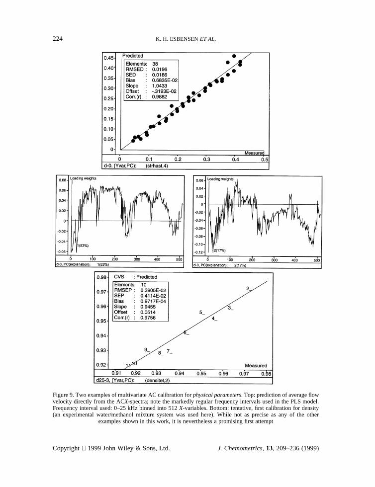
Figure 9. Two examples of multivariate AC calibration forphysical parameters. Top: prediction of average flowvelocity directly from the ACX-spectra; note the markedly regular frequency intervals used in the PLS model.Frequency interval used: 0–25 kHz binned into 512X-variables. Bottom: tentative, first calibration for density(an experimental water/methanol mixture system was used here). While not as precise as any of the other

examples shown in this work, it is nevertheless a promising first attempt



Any substance which similarly influences the surface tension of water will also make a contributiontowards changing the effective surface tension of the flowing mixture, be this in the form of anemulsion, a solution, etc. Actually, the exact physical form of the mixture is not of particular practicalinterest for the present applications point of view—so long as the AC principles work! This will ofcourse always be adequately assessed by the proper validation procedures for the predictivemultivariate calibration models developed.

Changing the effective surface tension of the flowing medium will be necessity also change theresulting turbulence vibration spectrum, as revealed by the FFT spectra. Even the small(est) change inthis full-spectrum signal is usually more than enough when subjected to a subsequent multivariatecalibration stage (PLS-R); witness, for example, the accuracy and precision obtained in Figures 8, 10and 11.

We are now in a position to start going for a more general understanding of the physical phenomenbehind the generation of selective turbulence spectra. In general the FFT transform delineation of theturbulence regimen will be a selective (though certainly not exclusive) reflection of

. the composition of the mixture/emulsion/slurry (composition influences the surface tension)

. the velocity of the emerging jet (influenced by the viscosity of the mixture)

. the temperature (influences the surface tension significantly)

. the density of the mixture/emulsion/slurry (partlyconfoundedwith the temperature influence).

These factors may easily be modelled by ‘inverse causal calibration’.11 If the pertinentX-spectra arecausally influenced by a specific of the above factors, it is easy to set up a corresponding multivariatecalibration model for this same factor. TheX-spectra arebona fidereflections of the pertinent factor’sinfluence—e.g. the concentration of a particular analyte—even though the detailed physicalmechanism may not be known (yet).

For this discussion, assuming constant temperature, constant flow velocity, constant density, etc.(all of which will not result in any loss of generality), a more fully developed understanding of thegeneral AC measurement principles opens up. Even though the actual data path for the signalsadmittedly is comparatively complex (Figure 4), it is by no means more complex than for manyother comparable measurement principles and their technical realizations.1 The physicalphenomenon modelled is here explicitly used in the ‘backward causal’ mode of Martens andNaes:11 indirect calibration. The AC approach makes use of all the full-spectrum advantagesavailable to multivariate instrumentation calibration. The compound but simple physical/engineering/data analysis context for the generation of this type of diagnostic spectrum will sufficefor broadening the understanding of the potential for still more general applications, e.g. forextending to other types of influencing analytes, or to several simultaneous analytes, or even tocalibration in the presence of active interferents.

Summing up, an acoustic chemometric phenomenological master equation (meaning that the FFTspectra are afunction of these factors—and probably more) can be written asFFT spectrum(X) = F (velocity, composition, temperature, density, OP configuration, …)This is to be relatedto the standard PLS-R data modelling master equationPLS-R: Y-parameter = PLS-R (FFT X-spectrum) Together these equations encompass many of the desired augmentation/extensionpossibilities sought. It may for example be appreciated how the AC principle (and instrumentation)can now be ‘tuned in’ forany of the influencing parameters in the first equation.

For example, this is why it comes as no surprise that thesame X-spectra used for trace oilquantification can also be used—simultaneously—for velocity calibration, as seen in Figure 9.Furthermore, it will also be apparent why there have been found found promising possibilities forother physical parameter quantification, e.g. density calibration, which is also depicted in Figure 9(though not fully explored yet).



Below follow still more demanding AC prediction tasks, first augmenting for quantitative chemicalconcentration calibration of fluid/fluid mixtures.

AC FOR JET-FUEL/GLYCOL-IN-WATER

Building on the satisfying results for oil-in-water determinations, the focus soon turned to

Figure 10. One-analyte calibration forjet-fuel (eight concentration levels); five replicate measurements at eachlevel. Cross-validation shows three PLS components optimal: approximately 63% of theX-variance is used toexplain 99% of theY-variance. Calibration range 0–100 ppm corresponds to the Norwegian Aviation Agency

authorities’ environmental monitoring requirements. Baseline jet-fuel study—no glycol present in system



environmental applications. Quantitative monitoring of environmentally harmful substances is also asituation in which the analyte (: harmful substance)-in-water often is the culprit one would like tomonitor, accurately, precisely and inexpensively (there aremanypollution point sources these days).While this is also an excellent opportunity for the kind of AC rig experimentation shown above in thelaboratory, direct in-field, routine applications are the ultimate goal. Similar measurement principlesusing e.g. a calibrated integrated nozzle/accelerometer unit can easily be envisaged, which has the

Figure 11. One-analyte calibration forglycol (eight concentration levels). Note drastically larger calibrationrange 0–3000 ppm (authorities’ environmental monitoring requirement for this analyte). Cross-validation; two

PLS components used. Baseline glycol study—no jet-fuel present in system



Figure 12.Two-analyte case(both jet-fuel and glycol present):jet-fuel calibration. Cross-validation leads to sixPLS components being optimal. Jet-fuel cannot be calibrated with comparable accuracy and precision (cf. Figure10) in this more restricted calibration range (0–60 ppm), but shows enough promising detail to merit further

R&D. Note how 80% of theX-variance actually explains 94% of theY-variance in this context



potential of being really inexpensive—an integrated nozzle/accelorometer/calibrated chip: a ‘smartsensor’ looms in the immediate future as a very desirable market issue.

Thus, as our second major example of the developments of acoustic chemometrics, we now presentselected highlights from the two-analytes-in-water regimen, as realized by ajet-fuel/glycol-in-watersystem. This system was also chosen for its direct application potential. Glycol is the main agent inde-icing sprays used on aeroplane surfaces before take-off in winter climates, and jet-fuel leakagesare to nobodys liking, so routine surveillance against these substances is naturally a must in anymodern airport environmental programme. Ultimately one would like to be able to measure each ofthese two contaminants, irrespective of the concentration of the other—preferentially with onesensor, if possible.

Initially the same HITAFF rig set-up as that for oil-in-water was used, and—interestinglyenough—only with a slightly different optimal velocity. In fact, the exact same orifice opening turnedout to be most useful also in this case. The main point of interest now is: can two simultaneouspredictive models be established?—and if yes, how well can the predictive abilities be compared withthose of the individual one-analyte models? This two-analyte-in-water problem might enter a regimenin which there may occur significantinteraction effectsbetween the two analytes themselves.A priorithere would not necessarily be any guarantee that their individual influence on the total systemsurface tension might also be individually decomposable, multivariate calibration notwithstanding.We decided to try our hands on full two-factor experiments with from six to eight levels for eachanalyte. While we have not yet solved all problems in this regimen, the results below neverthelessagain speak clearly for themselves to the trained chemometric eye (Figures 10–13).

On the basis of these four interrelated results, it can be concluded that there would not appear to beany very significantly harmful interacting effects—at least not in the jet-fuel/glycol-in-water system.As would be expected, a significantly larger number of PLS components are needed to model theY-variance in both the cases where two analytes are present simultaneously, but—most interestingly—the level to which theY-variance is modelled only shows a decrease by some 5%–10%, which is veryencouraging. Thismight bode well for the general possibilities for simultaneous multicomponentacoustic chemometric quantification, but it is of course early days yet, and many more studies areneeded. We may note though that a very satisfactory proportion of the totalX-variance available(65%–80%) is used in these AC calibrations. This strongly indicates that the present AC methodologyis already close to the target with respect to relevance and validity of theX-measuring technology alsofor this more complex system.

At this point in time we have initiated further similar investigations in order to start building up amore systematic experience, and already there are some salient questions emerging. What is thespecific nature of the analytes which lend themselves to be decomposable, i.e. which lend themselvesto such successful PLS1 calibration in the presence of other, similar analytes? Are there significantcommonalities between their chemical types?—or are there telling differences? What aboutinterferents?

ANALYTE(S)–INTERFERENTS: IS THERE A LIMIT TO AC?

The last example is designed to illustrate a still more complex situation, again with two (or evenmore) analytes present, but which is now augmented with active interferents, which arecertainalso toinfluence the surface tension of the total mixture. Initial collaborations with the Finnish RAISIOChemicals OY company have resulted in AC results for some selected ‘paper-pulp’ systems, whichindeed are very complex chemico-physical systems in relation to the above. The first results presentedbelow are representative for the kind of significant interaction that has to be addressed in this type ofindustrial system, and are thus—hopefully—able to reveal some insights into what, for the time



Figure 13.Two-analyte case(both jet-fuel and glycol present):glycol calibration. Glycol in this more demandingcalibration range (0–150 ppm) (cf. Figure 11) shows very promising prediction results; see statistics offittedregression line. Cross-validation leads to five PLS components optimal, at which 77% of theX-variance is used to

explain 94% of theY-variance



being, is by far the most complex AC system investigated so far. The main new factor in this system isthe presence of a significant proportion of solid particles in addition to the complex fluid mixtures.

Paper-pulp systems can—for the present purpose—be characterized (extremely simply) as verydilute water-based slurries, with about 2%–5% dry matter (paper fibres), in which an industry-relatedspecific set of chemicals (together with various physical characteristics of the colloidal systems aswell) are routinely measured in the analytical laboratory of many paper-mills and papermanufacturing plants—both for process monitoring and process control purposes, as well as forenvironmental protection purposes. There is a widespread interest in more easily obtainable analyses

Figure 14. Eleven-segment cross-validated multivariate calibration prediction for paper-pulp ‘component S’ inreference range 0–350 ppm. A five-component PLS model was found optimal. Note excellent predictionassessment statistics offitted regression line (r2 = 0⋅92, slope = 0⋅88) for this very complex system. Bottom:w1-

loading spectrum, showing many well-defined coherent frequency bands in the range 0–25 kHz



(routine monitoring—no laboratory) and/or in more rapid analytical results (in-line process control).We here limit ourselves to showing only one particular calibration, and for reasons that we have hadto cryptify the exact nature of the analyte in question, here we simply call it ‘component S’.

Figures 14 and 15 show the resulting AC calibration for component S, following the samemethodology as above, based on real-world paper-pulp mixtures prepared by RAISIO. The acousticchemometric analysis was again carried out on the HITAFF rig, of course now with the appropriatelyoptimized AC parameters for this system (different OP opening, flow velocity, etc.). Component Swas modelled for by using the ‘random design’ approach, as witnessed by the satisfactory spreadalong the calibration range in Figure 14.

Figure 15. (X,Y)-variance explained for paper-pulp ‘component S’ PLS model. A five-component PLS model isindicated by the validation. 92% of theY-variance is explained by (only) 45% of theX-variance, reflecting the

severecomplexityof this system



The dominant part of theY-modelling is due to the first PLS component, which neverthelessaccounts for only 22% of theX-variance. The particular (X, Y)-variance vs. number of PLScomponents plot shown in Figure 15 is archetypical of acomplex systembeing modelled by PLSregression. In this situation there is a lot ofX-variance captured by the AC (FFT) spectra which isnotcorrelated to theY-data (some 55% in fact). Thus even though component 2 increases theY-variancemodelled by almost 10%, for the three ‘extra’ PLS components (3–5) theY-prediction model onlygains some 5% additional variance explained collectively, while these four components togetheraccount for more than 30% of theX-variance. More than half of what has been captured by theacoustic sensor in this case is of no interest for component S whatsoever and is rightfully dischargedby the PLS model. Additional insight into this system comes from similar PLS models for a numberof other ‘significant pulp components’ (to be revealed in the nearer future). With these results, interestin further developing the AC approach for industrial use has received a very strong boost.

FUTURE RESEARCH

These satisfactory first results for a new measurement technique clearly meritsomeafterthought. Inour studies we have not only pursued the empirical application line exemplified above. Many morescientific questions appear on the agenda immediately.

. How is the ‘acoustic’ vibration generated in the first place: thephysicsbehind it all?

. How exactly are the ‘analytes’ causing the (composite) surface tension effects?

. What is thephysical reasonbehind the (apparent) decomposability of these compound effects?

. What are the systematics of successful applications?—which are the types of successfulanalytes?

. What are thelimits of AC applications?

We infer that a closer look at the details of the fluid dynamics of these augmented multicomponentOP systems will prove advantageous, especially when contemplating what modifications might becalled for in order to tackle even more complex physico-chemical systems; for example, mixtureswith multicomponent concentrations all well above the trace levels, say at 10%–30% concentrationsfor each component (analyte), or systems with similarly high concentrations of interferents. Surely alimit exists for what complexity can be tackled by AC.

A fundamental understanding of the physics behind the vibration generation (the physics/fluiddynamics behind the generation of the turbulence from the orifice plate downstream) is absolutelyessential. How come one is able also to pick up diagnostic vibrations alreadyat the constricting OPelement itself (Figures 6 and 7) when it was originally believed that the turbulence principally sets infirst at thevena contracta? For this kind of study,M. Halstensenconstructed thegradientOP systemdepicted in Figure 16. This device allows detailed study of several combinations of flow direction andmultisensor deployment.

The frequency spectrum (loading weights) of the successful PLS models carries a lot ofinformation related to these questions. The physical interpretation of such decomposed spectra is notstraightforward, since they are dependent on all the above influencing factors, and it is very prematurehere to go into these matters at any length. We may only point—quite descriptively—to a fewcomparative results, as seen by the loading weight spectra for the three major applications discussedin this paper. The first two, oil-in-water and jet-fuel/glycol-in-water, are perhaps the most comparableset-ups, as they pertain to very similar AC recording conditions (same OP configuration, rel. identicalapproach velocity, same temperature regimen), but of course these are twovery differentchemicalsystems in themselves. Figures 8, 10 and 11 detail that these two types of loading weight spectraindeed are not particularly similar (althoughsomeinteresting commonalities may seem to exist),



illustrating that this endeavour in all likeliness is not going to be simple. By a final comparison,Figures 12–14 actually show somewhat more similarw1-spectra for these (much more) complex two-analyte (many-analyte) systems—even though here also more complex patterns emerge which are notimmediately open to interpretations. One must not be discouraged, however—these are so differentsystems with so many experimental factors differing that similarities are absolutely not to be expectedin abundance here. What are called for are of course systematic studies, using strictly definedexperimental designs which allow for more direct and thus more meaningful comparisons to be made.

For this type of interpretative study the distribution of the most influencing frequencies in the rangeinvestigated here, 0–25 kHz, is but a coarse reflection of the details of the physics behind the quasi-chaotic hierarchy of superposed vibrational scales. Interpretation of the main operative ‘frequencybands’ will certainly have to go hand-in-hand with a deeper understanding of both the fluid dynamicsas well as the influencing agents responsible for the ‘diagnostic-selective’ modification of theturbulence phenomenon.

STOP PRESS

Initial numerical simulation studies (performed only after the first writing of this paper) would

Figure 16. Gradient orifice plate device (‘trumpet mouthpiece’), constructed byM. Halstensen, for more detailedstudies of the specifics of generation of AC turbulence. Note how reversal of flow directions will allowturbulence generationwithout the presence of back-circulation cells (in the ‘2’ flow direction) to be studied.Bottom: gradient OP device installed in ‘measurement zone 2' (cf. Figure 5), equipped with two accelerometers



indicate that the question of the orifice plate–turbulence relationships may soon well become lessenigmatic than what has been laid down as the basis for all the experimentalization reported above.There would appear to be good reasons to expect a ‘useful’ vibration coupling also to the orificeopening itself—besides downstream of thevena contracta. Alas, an already long enough paper doesnot allow further details here, but these results will of course be presented as quickly as possible.Figure 17, our very first computer simulation of the turbulence generation of a fluid passing throughthe present type of cylindrical orifice plate opening, will hopefully suffice to convince the reader thatthe turbulence regimen indeed would appear to be suitable for clamp-on acoustic chemometriccharacterization, from the orifice plate itself and several pipe diameters downstream—in excellentagreement with our empirical findings.

EPILOGUE

We have shown three major successful empirical multivariate calibration developments of the newacoustic chemometric principle at work—for quantification of concentration/mixture fractions ofcomponents in flowing fluids and mixtures. Along the way we have also obtained good evidence formany other potential targets for the same acoustic chemometric approach, such as density, velocityand flow regimen characterization. However, there is much more to be done. We believe that we havein fact witnessed the birth of a new, potentially widely applicable general technique,acousticchemometrics, destined to go far—in technology in general and in industrial applications inparticular—while there would also appear to be a broad academic challenge of more fundamentalstudies still to be pursued.

ACKNOWLEDGEMENTS

The following MSc (Eng) students are gratefully credited for their thesis efforts and countless hoursin our laboratories, but certainly also for their loyal and very friendly contributions to building upACRG. For the record, eleven out of the 14 MSc (Eng) theses below are in Norwegian, but all are onrecord at ACRG.

1995: Kent H. Hjelmen1996: Per Oswald, Paul-Erling Lia, Andre´ Bautz, Arild Saudland, Per-Einar Rosenhave, Thorbjørn

Lied1997: Birger Evensen, Jørild Svalestuen, Maths Halstensen;1998: Jørn Steinsletten, Anne Berdal, Magne Berge, Tore Gravermoen.

Bjørn Hope (Sensorteknikk A/S) is the inventor and sole holder of a world patent regarding thefundamental principles behind the concept for external quantitative characterization of in-line

Figure 17. Simulation of turbulence generation in half-width orifice plate with circular opening; contours showturbulence intensity (highest intensity = black). Simulation based on approach velocity equal to typical HITAFFstudies reported above. From left to right, observe that turbulence isalsodeveloped close to the orifice plate



mixtures flowing in pipelines as perturbed by an existing or forced ‘constricting construction detail’.ACRG gratefully acknowledges senior engineer Talleiv Skredtveit, machine-shop chief

extraordinaire (HIT-TF), for his invaluable involvement and never-ending help regarding theHITAFF rig in general, the gradient OP device in particular (Figure 16) and many, many othercontributions.

ACRG acknowledges part-funding for the HITAFF rig materials from HIT-TF as well as part-funding from the Royal Norwegian Research Council (NFR) for some of the studies reported here.We also thank Tel-Tek for organizational as well as economic help—dealing administratively withACRG is not easy, we know—and especially acknowledge managing director Ynge Stentun.

RAISIO Chemicals OY acknowledges funding from ‘BRITE-EURAM III program, project GreenPaper’, which in part lies behind the paper-pulp preliminary results shown above. Anne Norstro˜m isgratefully acknowledged for her valuable contributions to analysing both ‘Component S’ and manyother constituents.

Bang & Olufsen Technology A/S, Struer, Denmark is gratefully acknowledged for permission touse a modified version of an illustration as a basis for Figure 2 here—from a reproduction fromReference 17.

Professor Morten C. Melaaen (Telemark Institute of Technology, Institute of Process Technology)is gratefully acknowledged for permission to prepublish the results of his initial computer simulations(Figure 17). The results of this collaborative work will be presented elsewhere in full.

REFERENCES

1. J. P. Bentley,Principles of Measurement Systems, Longman, London (1995).2. K. H. Esbensen, M. Halstensen, T. T. Lied, A. Saudland, J. Svalestuen, S. de Silva and B. Hope, ‘Acoustic

chemometrics—from noise to information’,Chemometrics Intell. Lab. Syst.44, 61–76 (1998).3. A. J. Ward-Smith,Internal Fluid Flow, Clarendon Press, Oxford (1980).4. J. Hinze,Turbulence, 2nd edn, McGraw-Hill, New York (1975).5. P. P. Stein,A Physical and Physiological Basis for the Interpretation of Cardiac Auscultation: Evaluations

Based Primarily on the Second Sound and Ejection Murmurs, pp. 219–221, Futura, New York (1981).6. K. H. Esbensen, K. Hjelmen and K. Kvaal, ‘The AMT approach in chemometrics—first forays’,J.

Chemometrics, 10, 569–590 (1996).7. DAQ AT-MIO/AI E Series—User Manual, National Instruments Corp. (1996).8. LabVIEW1 4⋅0 for Windows 95—User Manuals, National Instruments Corp. (1996).9. G. E. P. Box, W. G. Hunter and J. S. Hunter,Statistics for Experimenters, Wiley, New York (1978).

10. I. C. Ifeachor and B. W. Jervis,Digital Signal Processing, a Practical Approach, Addison-Wesley, Reading,MA (1993).

11. H. Martens and T. Næs,Multivariate Calibration, Wiley, Chichester (1989) reprinted 1994.12. S. Wold, C. Albano, W. J. Dunn III, U. Edlund, K. H. Esbensen, P. Geladi, S. Helberg, E. Johansen, W.

Lindberg and M. Sjøstrøm, ‘Multivariate data analysis in chemistry’, inChemometrics, Mathematics andStatistics in Chemistry, ed. by B. R. Kowalski, pp. 17–95, Reidel, Dordrecht (1984).

13. P. Geladi and B. R. Kowalski, ‘Partial least squares regression: a tutorial’,Anal. Chim. Acta, 185, 1–17(1986).

14. K. Esbensen, S. Scho˜nkopf and T. Midtga˚rd, Multivariate Analysis—A Training Package, Camo AS,Trondheim (1994) (3rd printing 1998 ).

15. The UNSCRAMBLER—User Manual, Camo AS, Trondheim (1995).16. MODDE (Graphical Software for Design of Experiments), Umetri/Umetrics (1997).17. M. Sugawara, ‘Stenosis: theoretical background’, inBlood Flow in the Heart and Large Vessels, ed. by M.

Sugawara, F. Kajiya, A. Kitabatake and H. Matsuo, pp. 97–104, Springer, Tokyo (1989).



Acoustic chemometrics for fluid flow quantifications - II: a small constriction will go a long way

Documents

Transcript of Acoustic chemometrics for fluid flow quantifications - II: a small constriction will go a long way