A

WRITE UP

ON

PROPAGATION OF SOUND IN FLUIDS

BY

AJAYI DAVID OLUSHEYE ARC/04/3171AND

OYEGOKE ADENIYI SUNDAY ARC/04/3225

SUBMITTED TO

THE DEPARTMENT OF ARCHITCTURE,

SCHOOL OF ENVIRONMENTAL TECHNOLOGY,

FEDERAL UNIVERSITY OF TECHNOLOGY.

AKURE, ONDO-STATE.

COURSE TITLE-ENVIRONMENTAL CONTROL III (ACOUSTIC)

COURSE CODE-ARC 507

COURSE LECTURER-

PROF. O. O. OGUNSOTE.

MARCH 2009

TABLE OF CONTENTS

1.0 Introduction.

1.1 Sound propagation in fluid

2.0 The Propagation of Sound

3.0 Sound Propagation in a Cylindrical Duct with Compliant

Wall

3.1 Analysis

4.0 Fast Sound Propagation in Binary Fluid Mixtures

5.0 Speed of Sound in Fluid

6.0 Stagnation and Sonic Properties of Sound Waves

6.1 Case Study 1: Adiabatic Flow

6.2 Case Study 2: Sonic Flow (Ma=1)

7.0 Conclusions

References

1.0 INTRODUCTION

1.1 Sound propagation in a fluid

Sound waves are traveling pressure waves in a fluid (gas or

a liquid). Consequence of this is that

there can be no sound propagation in vacuum. We verify this

by showing that an otherwise noisy personal alarm device

becomes completely silenced when placed in a vacuum.

Corresponding to the pressure wave is a displacement wave

s(x-vt) of atoms from where they would be if there had been

no sound propagating. The relationship between the

displacement wave and the deviation from average pressure is

a characteristic property of the fluid:

Note that ds/dx rather than s appears on the right hand side

of the equation because ds/dx measures the deformation of

the fluid from equilibrium: A constant s simply corresponds

to an overall displacement of the fluid. The negative sign

is there because a contraction ds/dx<0 gives an increase in

pressure and thus a positive p. B is called the bulk modulus

of the fluid and has dimensions of a pressure. It can be

shown that

 

where

is the ratio of the constant pressure to the constant volume

specific heat. We shall return to Eq. 12 later in the

course.

To derive the wave velocity in a fluid we write Newton's

second law for a cylindrical slice of thickness and area

A. The force on this slice is

We also calculate

Newton tells us to equate F and ma and this gives us the

wave-equation

From which we conclude that the speed of sound is

 

Neglecting the we could immediately have written down

this formula based on dimensional analysis or an analogy

with the previously derived expression for the wave-velocity

on a taut string. The formula was first derived by Newton

himself. Putting in numbers we get for air at ambient

pressure ( , , )

which is indistinguishable from the measured value

. Note that we have derived the interesting

result that at constant pressure the velocity of sound is

greater in a light than a heavy gas.

2.0 The Propagation of sound

Sound is a sequence of waves of pressure which propagates

through compressible media such as air or water. (Sound can

propagate through solids as well, but there are additional

modes of propagation). During their propagation, waves can

be reflected, refracted, or attenuated by the medium. The

purpose of this experiment is to examine what effect the

characteristics of the medium have on sound.

All media have three properties which affect the behavior of

sound propagation:

1. A relationship between density and pressure. This

relationship, affected by temperature, determines the

speed of sound within the medium.

2. The motion of the medium itself, e.g., winds.

Independent of the motion of sound through the medium,

if the medium is moving, the sound is further

transported.

3. The viscosity of the medium. This determines the

rate at which sound is attenuated. For many media, such

as air or water, attenuation due to viscosity is

negligible.

What happens when sound is propagating through a medium

which does not have constant properties? For example, when

sounds speed increases with height? Sound waves are

refracted. They can be focused or dispersed, thus increasing

or decreasing sound levels, precisely as an optical lens

increases or decreases light intensity.

One way that the propagation of sound can be represented is

by the motion of wave fronts-- lines of constant pressure

that move with time. Another way is to hypothetically mark a

point on a wave front and follow the trajectory of that

point over time. This latter approach is called ray-tracing

and shows most clearly how sound is refracted.

In the simulation which follows, the effects of the medium

on sound propagation can be visualized. The user can

generate a variety of sound-speed profiles and wind-speed

profiles by clicking on the profile choices and dragging the

red dots to establish amplitudes. Two sound sources are

available: a spherical source, in which initial sound waves

emanate uniformly in all directions; and a planar source, in

which initial sound waves emanate in a single direction. The

location of the source and it orientation can be changed by

dragging the red dots. Sound propagation in this simulation

is in two dimensions; and media profiles depend on height

only. Pressing 'Start' will begin the simulation.

Propagation is represented both by rays (black) and wave

fronts (red). Note that the sound speed C0 is artificially

low to accentuate the effects of the medium. (Sound speed in

air is nominally 340m/s; in water, 1500m/s.) Data, including

sound speed, wind speed, and derivatives, may be obtained by

clicking anywhere within the orange propagation field.

3.0 Sound propagation in a cylindrical duct with compliant

wall

There have been many applications that deal with sound

propagation in a compliant wall duct. These range from

hydraulic applications (i.e. water hammer) to biomechanical

applications (i.e. pressure pulse in an artery). In working

with sound propagation in a circular duct, the duct wall is

often assumed to be rigid so that any pressure disturbance

in the fluid has no effect on the wall. However, if the wall

is assumed to be compliant, i.e. wall deformation is

possible when a pressure disturbance is encountered, then,

this will change the speed of the sound propagation. In

reality, the rigid wall assumption will be valid if the

pressure disturbance in the fluid, which is a function of

the fluid density, is very small so that the deformation of

the wall is insignificant. However, if the duct wall is

assumed to be thin, i.e. ~ 1/20 of the radius or smaller, or

if the wall is made of plastic type of material with low

Young’s modulus and density, or if the fluid contained is

“heavy”, the rigid wall approximation is no longer true. In

this case, the wall is assumed to be compliant.

In the book by Morse & Ingard [1], the wall stiffness is

defined as K_w and this is the ratio between the pressure

disturbances, p, to the fractional change in cross-sectional

area of the duct, produced by p. Of course this pressure

disturbance p is not static and the inertial of the wall has

to be considered. Because the deformation of the wall is due

to the pressure disturbances in the fluid, this is a typical

fluid-structure interaction problem, where the pressure

disturbances in the fluid cause the structural deformation,

which in turn, modifies the pressure disturbances. Unlike

sound propagate in a duct with a rigid wall where sound

pressure travels down the tube axially; part of the pressure

is used to stretch the tube radially. Clearly, because of

the inclusion of tube wall displacement, this becomes a

fluid-structure interaction problem.

3.1 Analysis

In this analysis, it is expected that the speed of the

propagation will depend on the material properties of the

tube wall, i.e. Young’s modulus and the density. Also, as

the analysis unfolds, it will become apparently clear that

the speed of propagation will vary with excitation

frequency, unlike wave propagation in a rigid-wall tube.

Fluid

Two simplified fluid equations will be considered here:

and

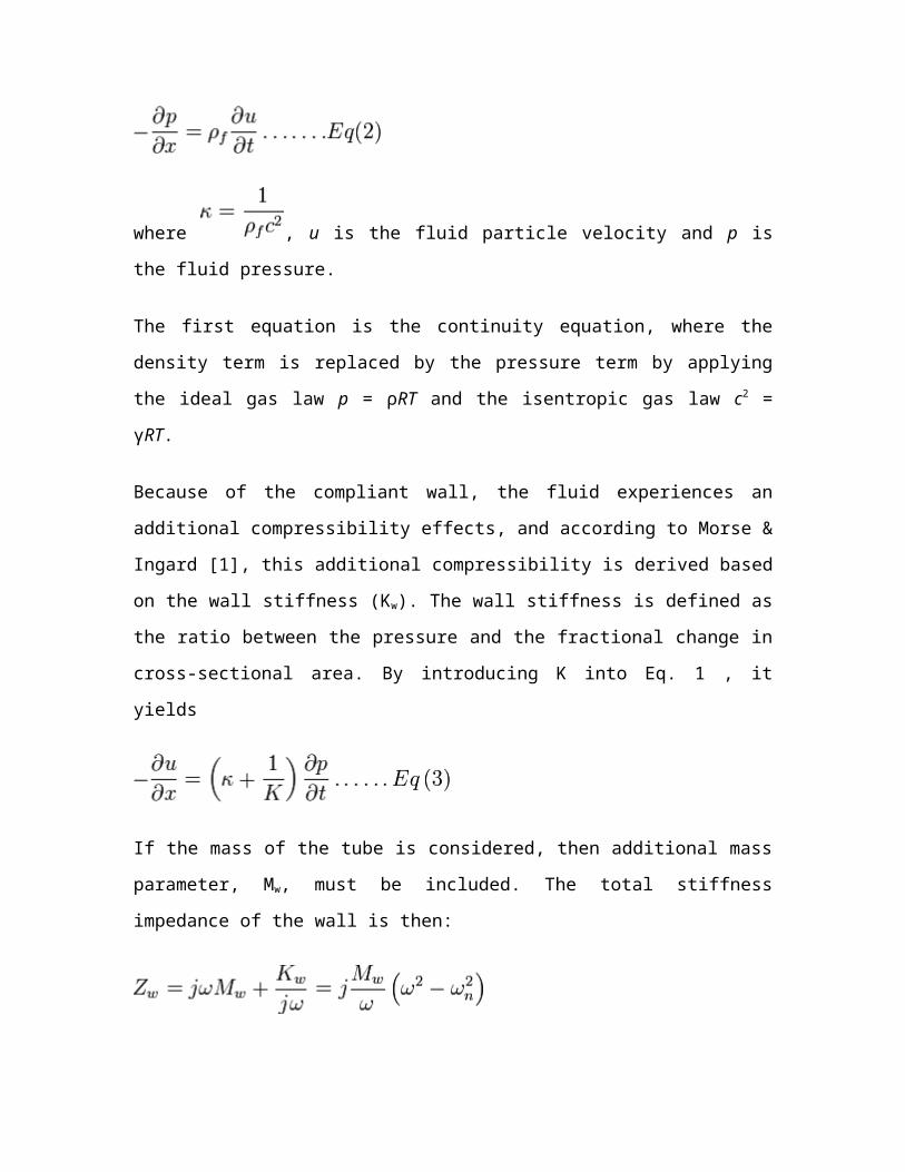
where , u is the fluid particle velocity and p is

the fluid pressure.

The first equation is the continuity equation, where the

density term is replaced by the pressure term by applying

the ideal gas law p = ρRT and the isentropic gas law c2 =

γRT.

Because of the compliant wall, the fluid experiences an

additional compressibility effects, and according to Morse &

Ingard [1], this additional compressibility is derived based

on the wall stiffness (Kw). The wall stiffness is defined as

the ratio between the pressure and the fractional change in

cross-sectional area. By introducing K into Eq. 1 , it

yields

If the mass of the tube is considered, then additional mass

parameter, Mw, must be included. The total stiffness

impedance of the wall is then:

Treating this wall impedance as a compliance term (i.e. K =

jω Zw), and substitute back into Eqn 3 yields

Here, .

Furthermore, by taking out kappa, the expression becomes

After some manipulation, it yields

Where

For rigid wall, as , , , hence,

, which leads back to Equation 1 .

If the impedance analogy is used, i.e. pressure is the

voltage and the velocity the current, then

, where C is the compliance of the wall per

unit length.

The speed of the sound is then determined by , hence

Here, cp is the phase velocity and it depends on the

excitation frequency, ω, the acoustic wave is dispersive.

When the excitation frequency is below the natural

frequency, ωn, the phase speed is lower than that of the

free wave speed in fluid.

The next step is to identify Kw and Mw, which will be

determined through structural response.

Structure

Assume the under formed tube has a diameter of D and after

deformation, it becomes . The area change in this

case is . The ratio between the two is

. Hence, the wall stiffness is then

.

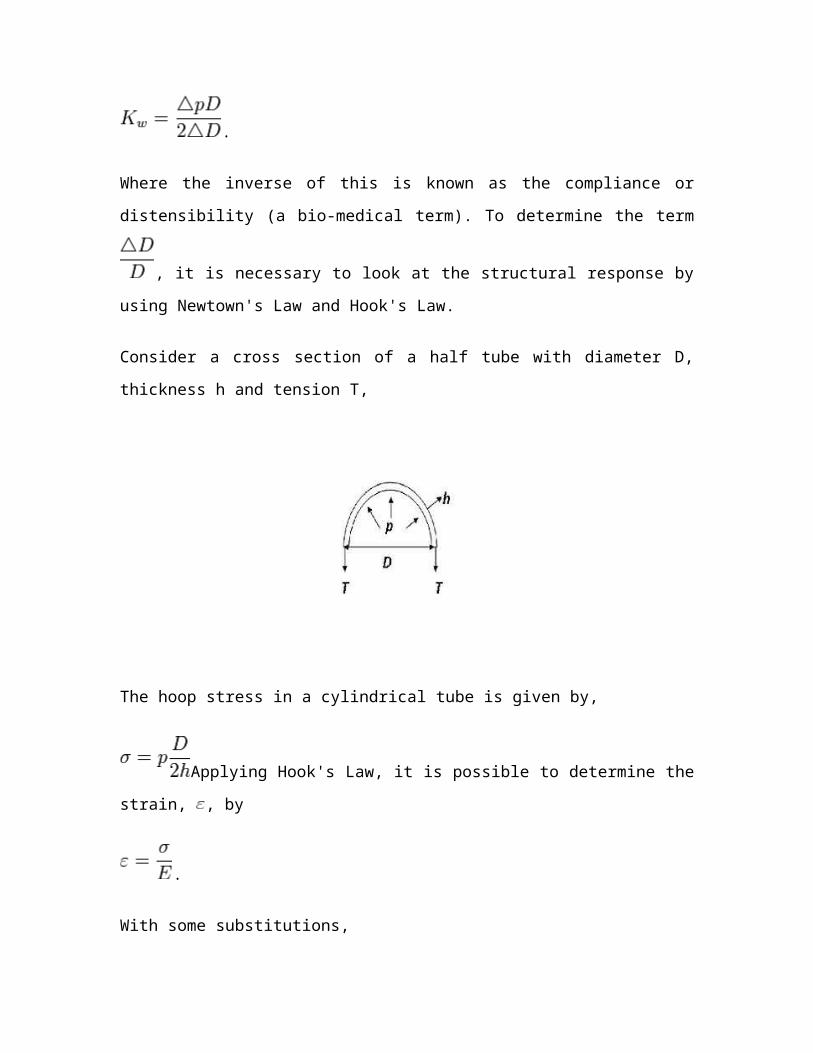
Where the inverse of this is known as the compliance or

distensibility (a bio-medical term). To determine the term

, it is necessary to look at the structural response by

using Newtown's Law and Hook's Law.

Consider a cross section of a half tube with diameter D,

thickness h and tension T,

The hoop stress in a cylindrical tube is given by,

Applying Hook's Law, it is possible to determine the

strain, , by

.

With some substitutions,

For small strain,

Hence,

This is the wall stiffness, a function of only the tube

elastic properties.

Mass of the tube per unit length is considered, then

Mw = ρsπh(D + h)

Finally, it is possible to plot the phase speed and the wall

impedance verse the excitation frequency.

Discussions

In the simulation the thickness to diameter ratio, is 0.1,

the material is steel with and E = 2x1011Pa. The

fluid contained inside is assumed to be air with

and the free wave speed of .

In this diagram, the 'o' denotes the real part of the phase

speed and the '+' denotes the imaginary part of the phase

speed. The straight line shows the sound speed in air with a

numerical value of . In this plot, propagation of

wave is possible only if the phase speed is real. There are

two important frequencies that deserve a close attention.

The first is the natural frequency of the empty structure,

i.e. ωn and the natural frequency of the fluid loaded

structure, ω1. In this plot, ωn = 450Hz while ω1 = 550Hz.

Unlike 1-D wave propagation in a rigid duct where the

propagation speed is a constant, the phase speed depends on

the excitation frequency. It shows that the propagation

speed decreases as the excitation frequency approaches to

ωn. Between ωn and ω1, the phase speed is imaginary, which

means no wave can propagate in between these two

frequencies. As soon as the frequency increases pass ω1, the

phase speed is greater than the free wave speed of 343 m/s.

As the excitation frequency increases, the phase speed

approaches to the free wave speed.

When the excitation frequency is increased, the parts of the

fluid energy are used to excite the tube, until the

excitation frequency matches ωn. Beyond ωn, no true wave

propagation is possible because in between these two

frequencies.

For a very rigid tube, i.e. E = 2x1020Pa , the phase speed is

exactly the free wave speed in air, which is a constant.

This agrees with what have been discussed before for a 1-D

wave propagation in a rigid duct.

When the stiffness is reduced to 1/100 of the steel, there

are numerous differences than the steel tube. First, at the

low frequency, the phase speed is slower. This is because

the lower wall stiffness, the more the wall can be

stretched, hence can absorb more energy. Also, the system

has a much lower ωn and ω1.

From the above analysis, it is possible to conclude the

following:

1. The stiffness, the wall thickness and the density of the

tube affects the phase speed dramatically.

2. A reduction in stiffness reduces the propagation speed at

low frequencies. The wave also becomes evanescent at much

lower frequency. This is because the natural frequency is

reduced. As the stiffness increases, the propagation speed

approaches to that of the free wave speed regardless of the

frequency region. This is the case of rigid wall.

3. The propagation speed of a wave in a duct with compliant

wall is dispersive as it depends greatly on the frequency.

The phase speed differs significantly than that of in a

rigid wall.

4.0 FAST SOUND PROPAGATION IN BINARY FLUID MIXTURES

Binary fluid mixtures are fluids consisting of two

different components. As for simple (one component) fluids,

the main experimental probes for the study of these

properties of binary mixtures are light and neutron

scattering. To connect the dynamics with scattering

experiments one can use the kinetic theory of fluids. I have

applied the kinetic theory to binary mixtures where the

atomic masses of the molecules of the two components are

very different (disparate-mass binary mixtures). I have

studied both dilute (gaseous) mixtures and dense mixtures.

In the description of the dynamics of the fluid through the

density-density correlation functions, one can introduce

modes, which can be thought of as the different channels by

which the correlations decay in time. Some modes are

propagating, in the sense that they describe propagating,

and damped processes. Others are not propagating, and

describe diffusive, purely damped processes. The results

concern the appearance of a fast propagating mode, in

disparate-mass binary mixtures, in a vast range of

densities, from dilute gas mixtures to rather high (liquid)

densities. This fast mode appears beyond the hydrodynamic

regime. One can call this mode fast sound, because, like

ordinary sound, it propagates, but it is faster. The most

important point is that the fast sound is associated with

dynamics of the light component only. In the thesis I

explain how this phenomenon could be observed in light and

neutron scattering experiments. If it is detected in actual

scattering experiments on disparate-mass binary mixtures it

would be the first time that a non hydrodynamic mode in a

fluid is clearly "seen".

5.0 SPEED OF SOUND IN FLUID

The so-called sound speed is the rate of propagation of a

pressure pulse of infinitesimal strength through a still

fluid. It is a thermodynamic property of a fluid.

A pressure pulse in an incompressible flow behaves like that

in a rigid body. A displaced particle displaces all the

particles in the medium. In a compressible fluid, on the

other hand, displaced mass compresses and increases the

density of neighboring mass which in turn increases density

of the adjoining mass and so on. Thus, a disturbance in the

form of an elastic wave or a pressure wave travels through

the medium. If the amplitude and therefore the strength of

the elastic wave is infinitesimal, it is termed as acoustic

wave or sound wave.

Figure 39.1(a) shows an infinitesimal pressure pulse

propagating at a speed " a " towards still fluid (V = 0) at

the left. The fluid properties ahead of the wave are p,T and

, while the properties behind the wave are p+dp, T+dT and

. The fluid velocity dV is directed toward the left

following wave but much slower.

In order to make the analysis steady, we superimpose a

velocity " a " directed towards right, on the entire system

(Fig. 39.1(b)). The wave is now stationary and the fluid

appears to have velocity " a " on the left and (a - dV) on

the right. The flow in Fig. 39.1 (b) is now steady and one

dimensional across the wave. Consider an area A on the wave

front. A mass balance gives

Fig 1.1: Propagation of a sound wave

(a) Wave Propagating into still Fluid        (b) Stationary

Wave

This shows that

        (a) if dρ is positive.

        (b) A compression wave leaves behind a fluid moving

in the direction of the wave (Fig. 1.1(a)).

        (c) Equation (1.1) also signifies that the fluid

velocity on the right is much smaller than the wave speed "

a ". Within the framework of infinitesimal strength of the

wave (sound wave), this " a " itself is very small.

Applying the momentum balance on the same control

volume in Fig. 1.1 (b). It says that the net force in

the x direction on the control volume equals the rate

of outflow of x momentum minus the rate of inflow of x

momentum. In symbolic form, this yields

In the above expression, Aρa is the mass flow rate. The

first term on the right hand side represents the rate of

outflow of x-momentum and the second term represents the

rate of inflow of x momentum.

Simplifying the momentum equation, we get

If the wave strength is very small, the pressure change is

small.

Combining Eqs (1.1) and (1.2), we get

The larger the strength of the wave, the faster the

wave speed; i.e., powerful explosion waves move much faster

than sound waves. In the limit of infinitesimally small

strength, we can write

Note that

(a) In the limit of infinitesimally strength of sound wave,

there are no velocity gradients on either side of the wave.

Therefore, the frictional effects (irreversible) are

confined to the interior of the wave.

(b) Moreover, the entire process of sound wave propagation

is adiabatic because there is no temperature gradient except

inside the wave itself.

(c) So, for sound waves, we can see that the process is

reversible adiabatic or isentropic.

So the correct expression for the sound speed is

For a perfect gas, by using of , and , we

deduce the speed of sound as

For air at sea-level and at a temperature of 150C, a=340

m/s

6.0 STAGNATION AND SONIC PROPERTIES OF SOUND WAVES

The stagnation properties at a point are defined as

those which are to be obtained if the local flow were

imagined to cease to zero velocity isentropically. As

we will see in the later part of the text, stagnation

values are useful reference conditions in a

compressible flow.

Let us denote stagnation properties by subscript zero.

Suppose the properties of a flow (such as T, p , ρ etc.) are

known at a point, the stagnation enthalpy is, thus, defined

as

Where h is flow enthalpy and V is flow velocity

For a perfect gas , this yields,

Which defines the Stagnation Temperature

Now, can be expressed as

Since,

If we know the local temperature (T) and Mach number (Ma) ,

we can find out the stagnation temperature T0 .

Consequently, isentropic(adiabatic) relations can be

used to obtain stagnation pressure and stagnation

density as

Values of and as a function of Mach number can

be generated using the above relationships and the tabulated

results are known as Isentropic Table .

Note that in general the stagnation properties can vary

throughout the flow field.

Let us consider some special cases:-

6.1 Case study 1: Adiabatic Flow:

(From eqn 1.1) is constant throughout the flow. It

follows that the are constant throughout an adiabatic

flow, even in the presence of friction.

Hence, all stagnation properties are constant along an

isentropic flow. If such a flow starts from a large

reservoir where the fluid is practically at rest, then the

properties in the reservoir are equal to the stagnation

properties everywhere in the flow Fig (2.1)

Fig 2.1: An isentropic process starting from a reservoir

6.2 Case study 2: Sonic Flow (Ma=1)

The sonic or critical properties are denoted by asterisks:

p*, ρ*, a*, and T* . These properties are attained if the

local fluid is imagined to expand or compress isentropically

until it reaches Ma = 1.

Important-

The total enthalpy, hence T0 , is conserved as long as the

process is adiabatic, irrespective of frictional effects.

From Eq. (2.1), we note that

This gives the relationship between the fluid velocity V,

and local temperature (T), in an adiabatic

Considering the condition, when Mach number, Ma=1, for a

compressible flow we can write from Eq. (40.2), (40.3) and

(40.4),

For diatomic gases, like air , the numerical

values are

The fluid velocity and acoustic speed are equal at

sonic condition and is

0r

7.0 CONCLUSION

An understanding of the nature of sound waves is

essential to discussion on acoustics. Sound waves are

longitudinal waves originating from a source and conveyed by

a medium. Sound is a disturbance, or wave, which moves

through a physical medium (such as air, water or metal) from

a source to cause the sensation of hearing in animals. Sound

is the sensation of the medium acting on the ear. The source

can be a vibrating Solid body such as the string of a guitar

or the membrane of a drum, but it can also be a vibrating

gaseous medium, such as air in a whistle. The medium may be

either a fluid or a solid.

18

REFERENCES

Morse & Ingard (1968): "Theoretical Acoustics", Princeton

University Press, Princeton, New Jersey

Aments, W. S., (1953): Sound Propagation in Gross

Mixtures. Acoustic. Sot.

Amer., v.25.P.638.

Biot, M. A., (1956a): Theory of Propagation of

Elastic waves in a Fluid-

Saturated Porous Solid, Part I: J.

Freudenthal, A. M., (1958): The Mathematical Theories of

the Inelastic Continuum,

First Part: Encyclopedia of physics,

v.6, p.267.

"http://en.wikibooks.org/wiki/engineering acoustics/sound

propagation in a cylindrical duct with compliant wall