A WAVE MODEL FOR SIMULATING VESSELEFFECTING SHALLOW WATER WAVES IN A

MARITIME SIMULATOR

Shabir MohamedUniversity of ColomboSchool of Computing

University of Colombo - Sri Lankahttp://www.ucsc.cmb.ac.lk

Email: shabir.tck@gmail.com

Dr. Chamath KeppitiyagamaUniversity of ColomboSchool of Computing

University of Colombo - Sri LankaEmail: chamath@ucsc.lk

Mr. Damitha SandaruwanModelling & Simulation Group

University of ColomboSchool of Computing

University of Colombo - Sri LankaEmail: dsr@ucsc.lk

Abstract—In modeling of the ocean wave effects in a MaritimeSimulator, the area of shallow water waves has taken precedencein recent times. Our study experiments the possibilities ofovercoming the barrier of high computation shallow water wavemodels that cannot be used for real time applications. Quotingfrom literature there exists three main approaches to model oceanwaves: 1) Geometrical Description Models, 2) Spectral Models &3) Physical based numerical models. The interest of this researchis towards models that are able to achieve high accuracy in termsof the wave properties; thus allowing to accurately depict waveconditions. It is the approach of numerically solved physical basedmodels (from those mentioned above) that can solve for waveparameters with high accuracy. The challenge imposed by suchaccurate models is the computation complexity that results in longprocessing time. Hence, they are not the most suitable choice forreal-time simulators. Our study experiments the possibility ofa solution to this problem by restricting the simulation area toonly that which has an impact on the vessel and by introducingcell reductions. The results obtained within the duration of thisstudy, reveal that maintaining an optimal accuracy with suchmesh-restrictions is not feasible and further efforts needs to beput in terms of parallel/gpu processing, profiling & etc.

I. INTRODUCTION

Since the advent of high order computation and computergraphics, simulations of real world phenomena have taken tocontribute in many areas. Also, they have evolved to a level ofusage for making critical decisions, user training on sensitiveenvironments, strategic planning and efficient predictions etc.Consequently, the need for optimum accuracy & flawlessrepresentation arose. One important area of such simulationsis the field of Oceanography. The study of maritime environ-ments can be categorized into Natural Phenomena(Wind, Waveand Light effects) and Physical Elements(Vessels, Tug boats,Floating bodies, Oil refineries) in the ocean environment.On a next level when simulating ocean waves, we have thedivide between Deep Ocean Waves and Shallow WaterWaves. Given the complexity of fluid motions in the naturalworld, simulations in this discipline tend to be complicatednaturally[9].

A. Research Motivation

When it comes to maritime simulators, the key purpose isto train new pilots to get used to the marine environment atdifferent sea conditions. As a result they are expected to beable to judge the behavior of the sea surface, understand themotion of the vessel and to make appropriate decisions. Thesimulator ultimately serves the purpose of catering to the needfor a real-life experience of different scenarios for new & oldpilots. One such important scenario is the vessel motion andmaneuvering in shallow or depth effective water conditions.Given the effect of depth, on the energy carried by the shallowwater waves, changes in the depth can have huge impacts onthe wave parameters such as height and velocity. In a maritimesimulator which is tested in environments closer to shallowwave conditions, it is of importance to be able to get theseessential wave parameters right.

B. Research Scope

Simulations in itself has two different branches. Onefocuses on producing results that is perceptively very muchcloser to the real-world scenario whilst the objective of theother is to provide results that are numerically precise &accurate. As for simulations that are solely user-experiencecentered, the focus would be to achieve perceptively realis-tic output [Ex: Movies, PC/Console Games]. However, forscenarios where the simulation output is used for predictivedecision making and for subsequent simulations, accurateresults are expected. Hence for such cases, it is necessary toaccurately model the final outcome of the simulation. It isnoteworthy that the final output of the simulation is highlydependent on the underlying mathematical model that is usedto calculate the fundamental “wave properties” (i.e in the caseof Oceanographic modeling). These wave properties are thenused in the upper layers of the simulation to account for thevarious wave effects.

Our focus in this research is towards shallow-waterwave models that are used in maritime simulators. Suchmodels demand the accuracy (described above), given thattheir utility is towards sensitive decision making scenar-ios. Hence, our study is concentrated towards the various

underlying mathematical models that produces the wave prop-erties required in the modeling and simulation of the shallow-water surface. Quoting from literature there exists three mainapproaches to model ocean waves: 1) Geometrical Descrip-tion Models(constructed using periodic functions), 2) SpectralModels (using empirical data from Oceanic researches) &3) Physical based models (from Computational Fluid Dynam-ics(CFD) based on numerical models).

It is noteworthy that only the approach of numericallysolved physical based models (from the 3 approaches men-tioned above) can provide wave parameters with high accuracy.Hence, this experiment is constrained to such physically basednumerical models (based on CFD). The main focus of ourstudy is towards a wave model that considers ”depth” as anintegral parameter in its calculations. The challenge imposedby such accurate models is the computation complexity thatresults in long processing time. Hence, they are not the mostsuitable choice for real-time simulators. Upon successfullyimplementing our proposed “depth” effective shallow-waterwave model, we experiment its applicability towards real-timeexecution.

II. BACKGROUND

Ocean waves are primarily an effect of energy transmissionfrom atmospheric winds onto the water particles in the deepocean surface. The more specific shallow-water waves aregenerated as a result of this energy being conducted to theshore from the deep ocean waves. The Shallow Water Waveshas its unique characteristic of the depth of the water volumeeffecting the wave surface and hence, the wave motion too.The distinction between deep and shallow water waves hasnothing to do with absolute water depth. It is determinedby the ratio of the water’s depth to the wavelength of thewave. The change from deep to shallow water waves occurswhen the depth of the water, d, becomes less than one halfof the wavelength of the wave, λ. When d is much greaterthan λ/2 we have a deep-water wave or a short wave. Whend is less than λ/2 we have a shallow-water wave or a longwave[19]. Deep ocean waves can be predicted using thewave models developed based on fore-casted wind spread.These models are based on the equations from the laws ofconservation. Depth integrating these equations, produces themodel required for depth effective shallow water waves. Byadding the finite-depth effects of shoaling, bottom frictionand refraction shallow water waves can be simulated[3].

The numerical equations based on which the wave modelsare designed can be categorized according to how they arederived[7]:

• Models based on Potential Flow Theory: Green NaghdiEquations, Boussinesq Equations, Mild Slope Equations

• Models based on the Laws of Conservation: Energybalanced, Complete Navier-Stokes Equations

The models based on the potential flow theory can besolved much quickly with less computation power. However,this advantage is at the expense of the accuracy in the waveproperties; since these equations are derived under some closedcondition with several assumptions on the basic fluid motion

in concern. On the other hand, the Navier-Stokes Equations isvery powerful in terms of the numerical precision when solvedfor the wave characteristics. This in turn has the drawback oftaking very long execution time and computation power, giventhe complexity of these equations.

A. Shallow-Water Equations

There term Shallow-Water Equations is used in twodifferent contexts. The first is the shallow-water equationsderived from the basic principals of conservation of mass andmomentum with fluid height or depth as a dependant variable.The second is one which is derived from existing numericalmodels by integrating it over the depth field.

1) Derived from Mass & Momentum principals: Thisform of the shallow water equations are derived by applyingthe laws of conservation of mass and momentum over thedepth/height field of the water. This form of the equationis a very basic model and is not common in oceanographicmodeling of shallow-water waves.

2) Derived from existing numerical models: These mostcommon and realistic models used in maritime environmentsinclude terms that describe the topography of the ocean floor,the Coriolis force resulting the earth’s rotation and possiblyother external forces. These are models derived from theother sophisticated numerical equations(mentioned earlier).These equations are of two different types: Phase Averagedand Phase Resolving models.

• Phase Averaged Models: are obtained via extending theEnergy & Action balance equations by adding the requiredphysical processes. Examples of such models can be foundin [4]&[6]. The energy spectra of the wave are modeled,whilst the phases are assumed to be uniformly distributed.However, this method is numerically inefficient if theresults are used to account for non-linear wave effects[1].

• Phase Resolving Models: are based on the Mass & Mo-mentum balance equations. Since the phase information islost in a phase averaged models, phase resolving modelsare widely used and more preferred because their ability tocalculate accurate wave properties. Examples of these mod-els include ones that are based on Hamiltonian Equations([12][16]), Boussinesq Equations ([14][5][10]) and Mild-Slope Equations ([2][15][8]). Each of these phase-resolvingmodels have their own limitations. The mild-slope equationscan calculate efficiently regular waves, but it cannot dealwith irregular waves such as wind driven waves. On the otherhand, Boussinesq-type models are able to deal with irregularwaves over varying bathymetry and allowing nonlinearity,but these models are limited by their accuracy in dispersionrelation. In general they don’t support wave generationby wind and do not take ”depth” as a parameter in itscalculations.

In addition to these models, the Shallow-Water Equationscan be derived from the Navier-Stokes Equations as well.It is acquired by depth integrating the NSE. This derivationgives accurate results for the wave parameters over a chang-ing bathymetry. However, this model poses the problem ofcomputational expensiveness and as a result, long processingtime.

There exists multiple “Deep-Ocean-Wave” models devel-oped based on the Navier-Strokes Equations. Maheshya etal.[20] in their work have produced a hybrid approach tosimulate deep ocean waves in real time with sound math-ematical results. They have derived a mathematical modelfor wind generated waves via Computational Fluid Dynamicsmethods. However, there is still a void for “Shallow-Water-Wave” models based on the depth averaged Navier-Stokesequations. This is primarily because such models require theproper study of the scenario & the scope of its implementationand usage. Only a model bounded by a specific contextyields feasible to be used as an accurate model for shallowconditions; also can allow further investigation towards real-time application. In our study we design and implement a-depth averaged Navier-Stokes Equation- based “Shallow-Water-Wave” model and seek the possibilities of overcomingthe barrier towards real-time to some extent using possiblecell manipulation techniques.

III. DESIGN & IMPLEMENTATION

A. Design Assumptions

As discussed earlier the implementation of a Shallow-Water model has to be done in accordance to a specificcontext, so that we can experiment its capabilities towardsreal-time application. Hence the following design assumptionsare made with respect to the overall model:

• Wave generation is only an effect of the surface stressapplied by wind on the Deep ocean surface at sea states ofB-S ≤ 5.

• Shallow-Water waves are a result of Deep ocean Waveenergy propagating into shallower conditions.

• No energy is lost due to divergence or convergence of thewave.

◦ no energy loss due to bottom friction or viscouseffects

◦ no energy is lost/added by wind as the wavepropagates through shallow waters

• Vessel is aligned in a direction parallel to that in which thewave propagates.

• Simulation area does not contain a physical boundary - iscontinued by some ocean area.

The last two assumptions define the scenario in which themodel is to be set. We implement our model in an environmentof the harbor waiting area. In order to define & limit thearea of the simulation we study the distance from the vessel

up-to which the waves has an impact on the vessel. Thus wedefine our simulation space as a rectangular grid encompassingthe vessel (explained later). If we are to consider any vessel-alignment angle, then our rectangular shaped simulation areawould also differ accordingly. Consequently, the need risesto calculate different boundary conditions at every boundarypoint of the grid. This leads to an overhead of computationtime and space. Hence, we assume that the vessel is alwaysaligned parallel to the wave propagation direction making thesimulation grid unchanged with a uniform boundary layer. Wealso mention that the simulation space is not disturbed by anyphysical boundaries in order to negate the effects of reflectivewaves.

B. Scope Limitations

As per our objective to achieve real-time application ofthe model implemented, we consider the scope to be limitedto the following conditions.

• Layout of the model is restricted to only an area that has aneffect on the vessel

• Constant depth ocean bed (space near harbor waiting area)

• Flat bathymetry with no topological changes

• Sea states of Beaufort Scale ≤ 5

• Hull shape of the vessel is identical to a cuboid

These scope limitations are defined such that we reducethe complexity of the calculations. We implement our modelto have a constant depth grid. However, we have includedthe option of setting up of a sloping/gradient ocean bed ifnecessary in future. Also in the scope of our research, wehave left out all changes in the topology of the ocean bed andconsider it to be smooth. In addition, a cuboid-shaped vesselis considered in order to efficiently define the grid boundaries(explained later).

C. Shallow-Water Equations

The depth averaged Navier-Stokes Equations results in thefollowing, also known as the Shallow-Water Equation:

∂(hU)∂t +∇.(hUTU) + f ∗ hU = −|g|h∇(h+ h0 + 1

ρ [τs − τb + F ])

Note that this equation is derived taking into consideration theeffect of the “Coriolis force” due to earth’s rotation. Giventhat our simulation space is restricted to only a specific areaaround the vessel, the effects of this force is minute. This isbecause our simulation grid is very small compared to theearth’s surface and the duration of the simulation is limited.Hence, we do not take this force into consideration in ourmodel. In addition to this, we also reduce these equationsto not consider the effects of the surface stress(τ ) & bottomfriction(F ) as per our design assumptions. Thus, the equationused in our model reduces to:

∂(hU)∂t +∇.(hUTU) + hU = −|g|h∇(h+ h0)

D. Implementation Module

A suitable implementation platform had to be chosenfor our model. Our focus was keenly set towards availableCFD packages with the key consideration being towards thenumerical precision of any solver. Various such packages (Ex:Fenics Project, SU2, Freefem, Gerris, OpenFOAM, PyClaw,GeoClaw etc) were tried out before concluding on the choiceof OpenFOAM CFD Package. Two primary reasons for thischoice were:

1) OpenFOAM has an existing solver for transientShallow-Water Equations

2) Fully open-source and has an extensivedocumentation

E. Hardware

The experiments were carried out in an off the shelf PC,used for academic research at the University of ColomboSchool of Computing.

• Processor: Intel Core i7-3770, 3.4 Ghz Processor

• RAM: 8 GB

• Cache L3: 3MB

• GPU: Gallium 0.4 on NVE7

• Storage: 500 GB

F. Design Plan

Setting up of a Base Grid for the Wave Model

Changes to the Base grid and

extract the results

Analyse results for accuracy &

real-time capability

Shallow WaterWave Modelbased on N-S

equations

Pre-Simulation Case

The design process of our study took the flow portrayed above.We started off by studying the scenario-of-implementation ofour model. Based on this study we designed and implementeda Base Model to solve for wave properties in Shallow-Waterconditions. This Base Model was tuned to have the optimalsettings in accordance to the wave conditions at Beaufort Scale≤ 5. The result is our “Shallow-Water-Wave” model basedon the Navier-Stokes Equations with depth consideration. Asdepicted by the diagram above we have implemented a Pre-Simulation Model in order to calculate the accurate boundaryconditions to be set to our Base Model. The Pre-SimulationModel is designed in accordance to actual sea conditions inorder to deduce the boundary values precisely.

Upon successfully implementing the Base Model andvalidating the results produced for accuracy, we introducefurther modifications/changes to the settings of the model.

Subsequently, we experiment the modified model for run-time applicability. We also study the results produced toanalyze its deviation from the outputs of the Base Model.We carry out these modification-analysis steps iteratively toinfer the possibilities of achieving real-time capabilities whilstmaintaining the accuracy of the wave properties produced.

G. Model Setup

Harbor Waiting Area

70m

40mGrid

Structure Pier

d=30m d=20m d=15m

250m

d=Wavelength/2

Deep OceanState

Shallow WaterState

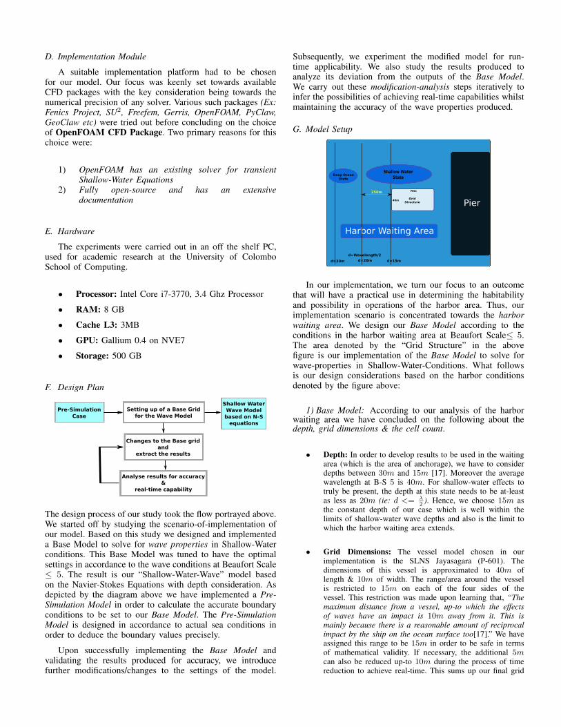
In our implementation, we turn our focus to an outcomethat will have a practical use in determining the habitabilityand possibility in operations of the harbor area. Thus, ourimplementation scenario is concentrated towards the harborwaiting area. We design our Base Model according to theconditions in the harbor waiting area at Beaufort Scale≤ 5.The area denoted by the “Grid Structure” in the abovefigure is our implementation of the Base Model to solve forwave-properties in Shallow-Water-Conditions. What followsis our design considerations based on the harbor conditionsdenoted by the figure above:

1) Base Model: According to our analysis of the harborwaiting area we have concluded on the following about thedepth, grid dimensions & the cell count.

• Depth: In order to develop results to be used in the waitingarea (which is the area of anchorage), we have to considerdepths between 30m and 15m [17]. Moreover the averagewavelength at B-S 5 is 40m. For shallow-water effects totruly be present, the depth at this state needs to be at-leastas less as 20m (ie: d <= λ

2). Hence, we choose 15m as

the constant depth of our case which is well within thelimits of shallow-water wave depths and also is the limit towhich the harbor waiting area extends.

• Grid Dimensions: The vessel model chosen in ourimplementation is the SLNS Jayasagara (P-601). Thedimensions of this vessel is approximated to 40m oflength & 10m of width. The range/area around the vesselis restricted to 15m on each of the four sides of thevessel. This restriction was made upon learning that, “Themaximum distance from a vessel, up-to which the effectsof waves have an impact is 10m away from it. This ismainly because there is a reasonable amount of reciprocalimpact by the ship on the ocean surface too[17].” We haveassigned this range to be 15m in order to be safe in termsof mathematical validity. If necessary, the additional 5mcan also be reduced up-to 10m during the process of timereduction to achieve real-time. This sums up our final grid

to be 70m long and 40m wide.

• Cell-Count: The cell count for the initial setup is fixed at 15cells per meter. This number is chosen such that the solverexecutes without failure/errors whilst an optimum level ofaccuracy can be reached with the calculations made. Setting15 cells/meter gives 1050(15 ∗ 70) cells along the length ofthe ship and 600(15∗40) cells along its width. A single layerof such a setup will be made up of an area of 630, 000 cells.

At sea states <= 5 in the B-S, the average wave length is39.7m and the average height is 1.8m [18]. If we considerapproximations of 40m and 2m respectively, then the heightvariation of the wave (assumed to be a sine curve) until 1

4(10m) of its wavelength is from 0m to 2m. This depicts thatthere is 0.2m of height gain at every 1m interval. Hence,we can conclude that on a grid with 15 cells/meter everycell on average would resolve a height of 0.2m

15= 1.33cm.

Increasing the value of cells/meter to 20 would result anincrease of approximately 490, 000 more cells per layer.This change effects the number of calculations per loop andsubsequently the overall complexity. On the other hand theheight resolution per cell only increases by a fraction to1cm from 1.3cm (a refinement of 3mm). If we pick a valuedouble of this (30cells/meter), then the height resolutionis refined only to 0.67cm whilst the no of total cells inthe grid increases by approximately 1, 890, 000. Hence, ourselection of 15 cells/meter is very efficient considering thetrade-offs between the accuracy gain by finer meshes andthe complexity to resolve them. In addition multiple runsof the initial case showed that the solver converged withoutany errors only at 15 cells per meter.

The figure above is a depiction of the grid setup of ourBase Model. Note that the depth of the simulation case isdenoted by a single cell of 15m in the z direction. The heightfields generated on each of these cells provide the heightof the wave at each point across the grid. In terms of thecomplexity of the calculations, it is the optimal choice whichgives us just a single layer grid. On the other hand in termsof the “effect on accuracy”, this approximation sets a constantvelocity at each point throughout the depth of the oceanfor 15m. In shallow water conditions the vertical pressuregradients are nearly hydrostatic, and horizontal pressuregradients are due to the displacement of the pressure surface,implying that the velocity field is nearly constant throughoutthe depth of ocean water [21]. Thus, the effects of taking asingle cell along the water depth is also justified.

2) Pre-Simulation Model: For successful execution of theBase Model it is necessary to accurately deduce its boundaryvalues. From the figure provided under Section G-Model Setup,we see that the area preceding the base grid structure from30m to 15m is part of the harbor waiting area. We recall thatshallow water conditions starts only at depths of 20m in seastates of Beaufort Scale ≤ 5 (i.e wavelength(40)

2 ). Thus, thepreceding 250m expanse of the ocean of our Base-Grid (asper the figure in section G) is to be treated to have shallow-water behavior whilst the rest is of deep-ocean. Hence, wedesign a Pre-Simulation Model (in accordance to the actualconditions of this 250m expanse of shallow-water) to deducethe boundary values for our Base Model in advance.

We have set the “mesh length” of the Pre-Simulation Model tobe 400m(> 250m) in length to ensure close-to-real depictionof the harbor environment. The values marked in red are onesthat define the mesh and the black ones denote the definitionof the case properties. As it is evident from the figure above,we have also designed this case to have a sloped bathymetryfrom the beginning of the grid up until the 250th meter wherethe depth reduces to 15m. The following 150m(400 − 250)is set to have a constant depth of 15m. Defining the depthto a uniform 15m after 250 meters in, is done to resemblethe actual scenario of our Base Model. Hence, the naturalbathymetry setting within the harbor waiting area is achievedby the above setup. We calculated the boundary values for thePre-Simulation Model based on the wave energy explanationsgiven in the studies of Mason et.al[11]. We also account forthe “influence of the modification in the particle flow patternon wave velocity in shallow-waters by the term

√tanh( 2πd

L )”.Thus, the boundary velocity of our Pre-Simulation Model isset to 5.88629ms−1.

We set the “timeStep(∆t)” for our simulations to be0.001s. Hence, data collected produces values for 1000 unitsin just 1 second. Also, a ∆t of 0.001s ensures a reasonablenumber of iterations per frame, when a single second isdivided into multiple frames. Finally, this value is well withinthe range of CFL ≤ 1. The CFL condition will not be negatedas long as the velocity does not increase by a factor of 10(which will not happen under the current sea state)[13].

With the above settings we executed our Pre-SimulationModel first. During its execution, we probed across the widthof the grid at 250m from the inlet (i.e the boundary of entryinto our Base Model) for the wave-properties produced. ThePre-Simulation Model was run for 90s(≈ 250m

5.88ms−1 × 2) togenerate boundary values of multiple wave trains for our Base

Model . We mapped the data collected from this execution tothe boundary of our Base Model . We then let the solver runover our Base Model for 1s with a write-interval of 0.04s. Thisis such that we can produce 25( 1

0.04 ) units of data which isequivalent to the framerate for real-time execution. We analyzewhether 1sec of the Base Model can be executed under 1secto produce 25 such data-units. If so we would have reachedreal-time capacities.

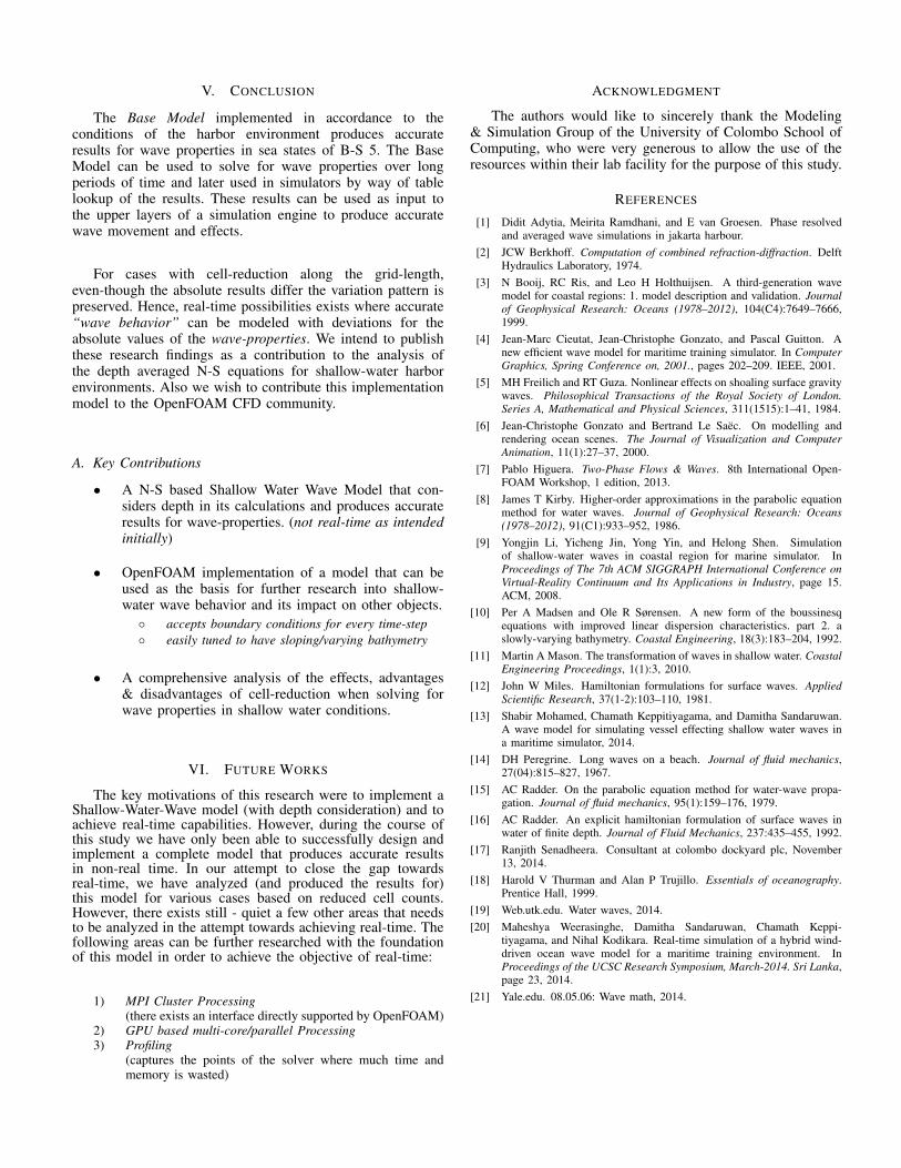
H. Cell-Reduction Mechanism

23.5 23.0 22.9 22.7 23.0 23.3 23.5 23.6 23.0 22.9 22.8 23.4 23.5 23.1 23.4 23.7

23.2 22.9 22.8 22.8 23.1 23.4 23.5 23.3 22.9 22.8 23.1 23.4 23.3 23.2 23.5

16

15

46.5

45.9

45.6

45.7

46.3

46.8

47.1

45.9

45.7

46.2

46.9

46.6

46.5

47.1

46.6divide by 2mask size = 2

Cell Count reduction: 15 -> 14Data Units: 16 -> 15

Reducing cell-count across the 40m width (wave inlet) of thegrid poses new challenges. Since our boundary values areuser-generated-values (from the outputs of the Pre-SimulationModel), we have exactly 16 units (16 units because: A cellcount of 15 per meter, means 16 edges all together. Hence wehave a data value at each of these edges.) of data per meter.Thus, reducing the no.of.cells per meter across the wave-inletdemands these values to be reduced to a scale equal to thenew no.of.cells per meter of the Base Model. We addressthis issue by introducing a simple convolution mechanismon the data points resulting from the Pre-Simulation Model.To reduce the cell count by 1 we introduce a mask of size2(1 + 1). We then slide the mask across an array of theoriginal values and average the units within the mask bythe length(2) of the mask. The no of resulting data valuesreduces by 1, when the mask has reached the end of the array.Please refer our thesis ([13]) for complete explanation of thealgorithm.

IV. RESULTS & EVAUATION

A. Pre-Simulation Model

The results for the wave-height variation at the 250m lineof the Pre-Simulation Model is given next. There is a linearincrease of the height field up until approximately 13.5s. Then,there is a sudden leap upwards to almost close to 24m. In thesubsequent time-steps, the height variation oscillates betweena max and a min value. The power of the energy transmittedat the Deep-Shallow water border is not completely felt at adistance as long as 250m initially. However, as a result ofenergy conduction between colliding adjacent water particlesa portion of this energy is felt at the 250m line. This energyincreases as the wave propagates in. As a result of this steadyincrease in the energy felt at the 250m mark, the wave heightis also seen to increase at a steady rate. Once the wave actuallyreaches our boundary of interest there is a sudden leap in theheight field. And then the total height continues to oscillates

between a maxima and a minima (similar to a wave). The totalheight does not fall back down to its original value because wehave multiple wave trains propagating inwards continuously.

0 5 10 15 20 25 30

1618

2022

2426

28

Variation of Wave Height at 250 meters

Pre−Simulation CaseTime

Tota

l Hei

ght

H = 2 − 3meters

0 5 10 15 20 25 30

02

46

8

Variation of Wave Velocity−X at 250 meters

Pre−Simulation CaseTime

Wav

e V

eloc

ity−

X

U = 7.85764ms−1

The figure above is a similar plot to show the variationof “wave velocity’s X-component” (i.e: component in thedirection towards the harbor) over time. The above also depictsthe same phenomena as to how the wave velocity varies withtime and goes by the same explanation.

• Wave Height: It can be observed in the formerfigure, that the difference between the “maximum”and the “minimum” values of the Total WaveHeight is between approximately 5 − 6 meters.Thus we have the actual Height of the wave to be≈ ( 5

2 −62 ) = (2.5 − 3) meters. This is exactly the

bounds of the upper limit for the Wave height atBeaufort Scale ≤ 5.

• Wave Velocity: The latter of the two figures depictsthat the Wave Velocity oscillates between the “mini-mum” of ≈ 3− 4ms−1 and the “maximum” velocityof ≈ 7 − 8ms−1. We substitute the upper-limits forwave properties in the sea states equal to B-S 5, onto the (Power=Energy*Velocity) equation explainedin [11],[13]. This calculation produces a velocity of7.85764ms−1. Hence, we see that our output forvelocity also falls within the upper range that definessea states of B-S ≤ 5.

B. Base Model

The red line is drawn across at 25m which is the approximateupper limit of all recorded heights and the green line at 21mwhich is the approximate lower limit. We see that the variationof the height field is always within these bounds. Thus, we caninfer that the maximum possible difference between any twowave crests is ≈ 25− 21 = 4m. So, the “upper bound” of thewave heights produced by the execution of our optimal BaseModel is 2m. By comparing this to the B-S table we ensurethat the results produced confirm to the actual height levels inB-S ≤ 5.

Note that, we are only interested in the maximum valuesfor velocity. As long as they confirm to the upper boundsof the sea-state of B-S ≤ 5, we are complacent. Hence weonly analyze the upper limits here. The red line denoting theupper limit(at B-S ≤ 5) is drawn across at 8ms−1. We seethat, the velocity is within this limit throughout the simulation.

C. Cell Reduced Execution

1) Cell Reduction along the grid-length:

We analyze each wave property by plotting its variation underthe optimal case & the cell-reduced case on top of each other.The optimal Base Case results are plotted in “black” and thecell-reduced case currently under consideration is plotted in“red”. By doing so, we examine how closely does the resultsof the cell-reduced case fits on top of the optimal Base Case.

This plot also allows us to get a graphical idea as to howsimilar the variation pattern of the property is (over time) inboth cases.

It can be noted (from the figure above) that the rangeslowly shrinks as the no.of.cells per meter along thegrid-length is reduced; thus showing a slight differencebetween the optimal case plot and the cell-reduced caseunder consideration. However, the most significant factthat we learn is that, the “red” plot continues to (almostalways) follow the same pattern as that of the optimal baseCase. Hence, we understand that even-though cell-reduction(along the grid-length) yields erroneous results in terms ofthe absolute height, the overall behavior (i.e height fieldvariation) of the wave property is preserved.

2) Cell Reduction along the grid-width:

We learn from the overlay graphs presented above, thatthere is a vast variation in the results produced for caseswhere the cell-count is modified across the grid-width. Thisis an expected outcome, because the boundary values usedfor these cases are not the original ones obtained from ourPre-Simulation Model. Rather, these are values produced bythe convolution of the original boundary data based on amask equal to the cell-reduction size.

D. Run-Time Analysis

Analysis of the run-time showed that there is an approxi-mate gain between 130s and 180s at every reduction of a singlecell (regardless of along which direction the cell-reduction wasdone). However, the gain as the cell-count is reduced from14 to 13 is higher than that of the rest. Moreover, even asthe cell-count is reduced to 1 cell along either of the grid-directions (length or width), the time taken for the solver torun to completion is still 105s ≈ 1min and 45secs. Thisdenotes the minimum duration to simulate 1sec of our BaseModel. Thus, we provide an analysis to the variation of wave-properties and the run-time caused by cell-manipulations onthe model. Please refer our thesis [13] for further explanationon the results obtained.

V. CONCLUSION

The Base Model implemented in accordance to theconditions of the harbor environment produces accurateresults for wave properties in sea states of B-S 5. The BaseModel can be used to solve for wave properties over longperiods of time and later used in simulators by way of tablelookup of the results. These results can be used as input tothe upper layers of a simulation engine to produce accuratewave movement and effects.

For cases with cell-reduction along the grid-length,even-though the absolute results differ the variation pattern ispreserved. Hence, real-time possibilities exists where accurate“wave behavior” can be modeled with deviations for theabsolute values of the wave-properties. We intend to publishthese research findings as a contribution to the analysis ofthe depth averaged N-S equations for shallow-water harborenvironments. Also we wish to contribute this implementationmodel to the OpenFOAM CFD community.

A. Key Contributions

• A N-S based Shallow Water Wave Model that con-siders depth in its calculations and produces accurateresults for wave-properties. (not real-time as intendedinitially)

• OpenFOAM implementation of a model that can beused as the basis for further research into shallow-water wave behavior and its impact on other objects.

◦ accepts boundary conditions for every time-step◦ easily tuned to have sloping/varying bathymetry

• A comprehensive analysis of the effects, advantages& disadvantages of cell-reduction when solving forwave properties in shallow water conditions.

VI. FUTURE WORKS

The key motivations of this research were to implement aShallow-Water-Wave model (with depth consideration) and toachieve real-time capabilities. However, during the course ofthis study we have only been able to successfully design andimplement a complete model that produces accurate resultsin non-real time. In our attempt to close the gap towardsreal-time, we have analyzed (and produced the results for)this model for various cases based on reduced cell counts.However, there exists still - quiet a few other areas that needsto be analyzed in the attempt towards achieving real-time. Thefollowing areas can be further researched with the foundationof this model in order to achieve the objective of real-time:

1) MPI Cluster Processing(there exists an interface directly supported by OpenFOAM)

2) GPU based multi-core/parallel Processing3) Profiling

(captures the points of the solver where much time andmemory is wasted)

ACKNOWLEDGMENT

The authors would like to sincerely thank the Modeling& Simulation Group of the University of Colombo School ofComputing, who were very generous to allow the use of theresources within their lab facility for the purpose of this study.

REFERENCES

[1] Didit Adytia, Meirita Ramdhani, and E van Groesen. Phase resolvedand averaged wave simulations in jakarta harbour.

[2] JCW Berkhoff. Computation of combined refraction-diffraction. DelftHydraulics Laboratory, 1974.

[3] N Booij, RC Ris, and Leo H Holthuijsen. A third-generation wavemodel for coastal regions: 1. model description and validation. Journalof Geophysical Research: Oceans (1978–2012), 104(C4):7649–7666,1999.

[4] Jean-Marc Cieutat, Jean-Christophe Gonzato, and Pascal Guitton. Anew efficient wave model for maritime training simulator. In ComputerGraphics, Spring Conference on, 2001., pages 202–209. IEEE, 2001.

[5] MH Freilich and RT Guza. Nonlinear effects on shoaling surface gravitywaves. Philosophical Transactions of the Royal Society of London.Series A, Mathematical and Physical Sciences, 311(1515):1–41, 1984.

[6] Jean-Christophe Gonzato and Bertrand Le Saec. On modelling andrendering ocean scenes. The Journal of Visualization and ComputerAnimation, 11(1):27–37, 2000.

[7] Pablo Higuera. Two-Phase Flows & Waves. 8th International Open-FOAM Workshop, 1 edition, 2013.

[8] James T Kirby. Higher-order approximations in the parabolic equationmethod for water waves. Journal of Geophysical Research: Oceans(1978–2012), 91(C1):933–952, 1986.

[9] Yongjin Li, Yicheng Jin, Yong Yin, and Helong Shen. Simulationof shallow-water waves in coastal region for marine simulator. InProceedings of The 7th ACM SIGGRAPH International Conference onVirtual-Reality Continuum and Its Applications in Industry, page 15.ACM, 2008.

[10] Per A Madsen and Ole R Sørensen. A new form of the boussinesqequations with improved linear dispersion characteristics. part 2. aslowly-varying bathymetry. Coastal Engineering, 18(3):183–204, 1992.

[11] Martin A Mason. The transformation of waves in shallow water. CoastalEngineering Proceedings, 1(1):3, 2010.

[12] John W Miles. Hamiltonian formulations for surface waves. AppliedScientific Research, 37(1-2):103–110, 1981.

[13] Shabir Mohamed, Chamath Keppitiyagama, and Damitha Sandaruwan.A wave model for simulating vessel effecting shallow water waves ina maritime simulator, 2014.

[14] DH Peregrine. Long waves on a beach. Journal of fluid mechanics,27(04):815–827, 1967.

[15] AC Radder. On the parabolic equation method for water-wave propa-gation. Journal of fluid mechanics, 95(1):159–176, 1979.

[16] AC Radder. An explicit hamiltonian formulation of surface waves inwater of finite depth. Journal of Fluid Mechanics, 237:435–455, 1992.

[17] Ranjith Senadheera. Consultant at colombo dockyard plc, November13, 2014.

[18] Harold V Thurman and Alan P Trujillo. Essentials of oceanography.Prentice Hall, 1999.

[19] Web.utk.edu. Water waves, 2014.[20] Maheshya Weerasinghe, Damitha Sandaruwan, Chamath Keppi-

tiyagama, and Nihal Kodikara. Real-time simulation of a hybrid wind-driven ocean wave model for a maritime training environment. InProceedings of the UCSC Research Symposium, March-2014. Sri Lanka,page 23, 2014.

[21] Yale.edu. 08.05.06: Wave math, 2014.