A variational method for the recovery of dense 3D structure from motion

Robotics and Autonomous Systems 55 (2007) 597–607www.elsevier.com/locate/robot

A variational method for the recovery of dense 3D structure from motion

Hicham Sekkati, Amar Mitiche∗

Institut national de la recherche scientifique, INRS-EMT, Place Bonaventure, 800, rue de la Gauchetiere ouest, Suite 6900, Montreal, Quebec, Canada, H5A 1K6

Received 3 March 2005; received in revised form 16 November 2006; accepted 16 November 2006Available online 19 December 2006

Abstract

The purpose of this study is to investigate a variational formulation of the problem of three-dimensional (3D) interpretation of temporalimage sequences based on the 3D brightness constraint and anisotropic regularization. The method allows movement of both the viewingsystem and objects and does not require the computation of image motion prior to 3D interpretation. Interpretation follows the minimizationof a functional with two terms: a term of conformity of the 3D interpretation to the image sequence first-order spatio-temporal variations, and aterm of regularization based on anisotropic diffusion to preserve the boundaries of interpretation. The Euler–Lagrange partial differential equationscorresponding to the functional are solved efficiently via the half-quadratic algorithm. Results of several experiments on synthetic and real imagesequences are given to demonstrate the validity of the method and its implementation.c© 2007 Published by Elsevier B.V.

Keywords: Image sequence analysis; Optical flow; 3D from 2D; Anisotropic regularization

1. Introduction

The recovery of the shape of real objects from imagemotion, referred to as structure from motion perception, is afundamental problem in computer vision. It occurs in manyuseful applications such as robotics, real object modeling, 2D-to-3D film conversion, augmented reality rendering of visualdata, internet and medical imaging, among others.

Computer vision methods which compute image motionbefore recovering structure are known as two-stage or indirectmethods. Those which compute structure without prior imagemotion estimation are known as direct methods. Direct methodsuse an explicit model of image motion in terms of the 3Dvariables to be estimated. For instance, in this study weassume that environmental objects are rigid and we expressimage motion in terms of the parameters of rigid motion anddepth.

One can also make a distinction between dense and sparserecovery of structure from motion. Sparse recovery, wheredepth is computed at a sparse set of points of the imagepositional array, has been the subject of numerous well-documented studies [1–5]. Dense recovery, however, where one

∗ Corresponding author.E-mail address: [email protected] (A. Mitiche).

0921-8890/$ - see front matter c© 2007 Published by Elsevier B.V.doi:10.1016/j.robot.2006.11.006

seeks to compute a depth and 3D motion over the whole im-age positional array, has been significantly less researched inspite of the many studies on dense estimation of image motion[6–8], understandably so, however, because practical applica-tions have appeared latterly.

This study addresses the problem of dense recoveryof structure from motion, more precisely the problem ofestimating dense maps of depth and 3D motion from a temporalsequence of monocular images. One must differentiate thisproblem from the problem of estimating depth in stereoscopy([9,10], for instance). Although one can argue that thetwo problems are conceptually similar because one can beconsidered a discrete version of the other, their input and theprocessing of this input are dissimilar. As indicated in [11],one can readily see a difference from an abstract point ofview, because stereoscopy implies the geometric motion ofdisplacement between views, and image temporal sequencesthe kinematic notion of motion of the viewing system andviewed objects. A displacement is defined by an initial positionand a final position, intermediate positions being immaterial.Consequently, the notions of time and velocity are irrelevant.With motion, in contrast, time and velocity are fundamentaldimensions. One can also readily see a difference from amore practical point of view, because both the viewing systemand viewed objects can move when acquiring temporal image

http://www.elsevier.com/locate/robot

mailto:[email protected]

http://dx.doi.org/10.1016/j.robot.2006.11.006

598 H. Sekkati, A. Mitiche / Robotics and Autonomous Systems 55 (2007) 597–607

sequences and all motions that occur enter 3D interpretation,which is not the case in stereoscopy. At the least, thisleads to computational complications. For instance, assumingthat environmental objects are rigid and images are sized640 × 480, there can be over 2 million variables to evaluateat each instant of interpretation (six for the screw of motionfunction and one for depth, an evaluation at each point of theimage positional array). The number of these variables canbe reduced if some form of motion-based segmentation enters3D interpretation [11,12]. Such a process, however, is itselfcomputationally quite intensive.

There are limitations common to all methods that seek a3D interpretation from a sequence of image spatio-temporalvariations:

(a) Because motion-based 3D interpretation requires percep-tion of motion, an obvious limitation is that such an inter-pretation is not possible when the surfaces to be interpretedare not in motion relative to the viewing system or havenon-textured projections, i.e., exhibit no sensible spatio-temporal variations. For such surfaces, depth is indetermi-nate unless propagated from neighboring textured surfaces.Regardless of how underlying computations manage inde-terminacy, schemes that aim to preserve the 3D interpre-tation boundaries prevent, to some extent, the propagationof interpretation to non-textured surfaces from neighboringtextured surfaces.

(b) To any interpretation consistent with a sequence, spatio-temporal variations corresponds a one-parameter family ofsolutions differing in scale.

(c) Direct implementation of a solution that refers to imagemotion presumes small-range motion. For large motions,some form of multiresolution processing must enter theinterpretation.

Within the general topic of motion analysis, relatively fewstudies have addressed the subject of dense 3D interpretationof temporal image sequences. Most of these do not allowfor object motion, assuming that the viewing system aloneis in movement [13–21]. As indicated in [11], when theviewing system moves but environmental objects do not, theproblem is simpler and 3D interpretation can be inferred by anindirect method which recovers depth following least-squaresestimation of 3D motion. The interpretation of scenes whereobject movement can occur was investigated in [11,12,22,23].

The variational method in [12] follows the minimumdescription length principle [24,25]. Environmental objects areassumed to be rigid, and this direct method seeks to partitionthe image domain into regions of constant depth and 3D motionby minimizing an objective function that measures the cost inbits to code the length of the boundaries of the partition andthe conformity of the 3D interpretation to the image sequencespatio-temporal variations within each region of the partition.The necessary conditions for a minimum of the objectivefunction result in a large-scale system of nonlinear equationssolved by continuation.

The purpose in [11] was to investigate joint rigid 3D-motionsegmentation and 3D interpretation by functional minimization.

The functional contained a term of conformity of the 3Dinterpretation to the image sequence spatio-temporal variations,a term of regularization of depth, and a term of regularityof segmentation boundaries. The Euler–Lagrange equationsof minimization were solved by an iterated greedy algorithmwhich included active curve evolution and level sets.

The purpose of this study is to investigate a new varia-tional method of 3D interpretation of image sequences, intro-duced briefly in [26], which brings to bear the anisotropic reg-ularization theory developed in [7] for image motion estima-tion by a variational method. The formal analysis in [7] de-termined diffusion functions from anisotropic smoothing con-ditions which preserved image motion boundaries. The anal-ysis also led to the half-quadratic algorithm for solving effi-ciently the equations of the variational image motion estima-tion method. Here we present a direct method of 3D interpreta-tion of temporal image sequences based on the minimizationof an energy functional containing two characteristic terms:one term evaluates the conformity of a rigidity-based 3D inter-pretation to the sequence spatio-temporal variations; the otheris an anisotropic regularization term on 3D interpretation us-ing the Aubert function. Minimization of the objective func-tional follows the Euler–Lagrange equations solved via the half-quadratic algorithm adapted to these equations. The method al-lows movement of both the viewing system and environmentalobjects as in [11,12]. It generalizes [26] to general rigid motion,relaxes the assumption of piecewise constant 3D variables [12],and is an alternative to level sets [11] of significantly lowercomputional cost.

The remainder of this paper is organized as follows. Inthe next section we describe the imaging model and statethe equations of the motion field induced by rigid motion.From these, we write the brightness constraint equation tobe used subsequently. Section 3 is devoted to recovering the3D interpretation for the case of a translational 3D motion.Section 4 generalizes the method for general rigid motion,resulting in a model for solving the most general case: arbitrarymotion of a viewing system relative to an environment ofmoving rigid objects. Section 6 describes several experimentalresults with both synthetic and real image sequences.

2. Rigidity-based constraint equation of direct methods

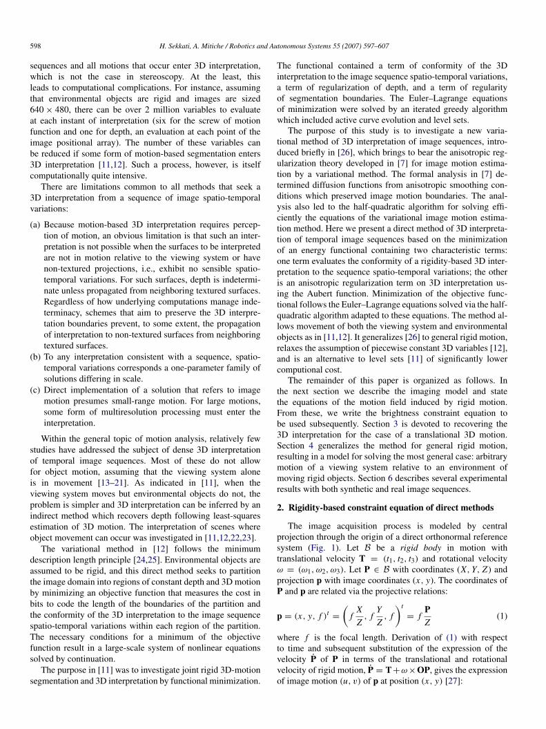
The image acquisition process is modeled by centralprojection through the origin of a direct orthonormal referencesystem (Fig. 1). Let B be a rigid body in motion withtranslational velocity T = (t1, t2, t3) and rotational velocityω = (ω1, ω2, ω3). Let P ∈ B with coordinates (X, Y, Z ) andprojection p with image coordinates (x, y). The coordinates ofP and p are related via the projective relations:

p = (x, y, f )t =

(f

X

Z, f

Y

Z, f

)t

= fPZ

(1)

where f is the focal length. Derivation of (1) with respectto time and subsequent substitution of the expression of thevelocity P of P in terms of the translational and rotationalvelocity of rigid motion, P = T+ω×OP, gives the expressionof image motion (u, v) of p at position (x, y) [27]:

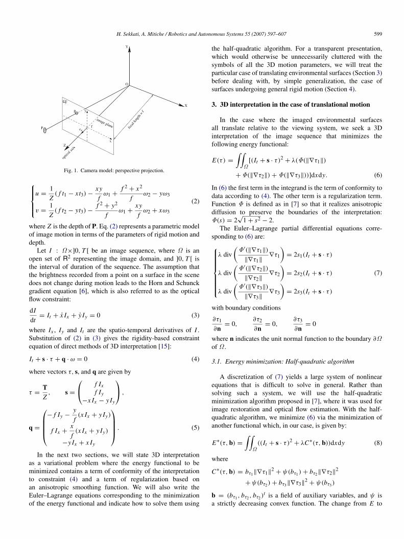
H. Sekkati, A. Mitiche / Robotics and Autonomous Systems 55 (2007) 597–607 599

Fig. 1. Camera model: perspective projection.

u =

1Z( f t1 − xt3)−

xy

fω1 +

f 2+ x2

fω2 − yω3

v =1Z( f t2 − yt3)−

f 2+ y2

fω1 +

xy

fω2 + xω3

(2)

where Z is the depth of P. Eq. (2) represents a parametric modelof image motion in terms of the parameters of rigid motion anddepth.

Let I : Ω×]0, T [ be an image sequence, where Ω is anopen set of R2 representing the image domain, and ]0, T [ isthe interval of duration of the sequence. The assumption thatthe brightness recorded from a point on a surface in the scenedoes not change during motion leads to the Horn and Schunckgradient equation [6], which is also referred to as the opticalflow constraint:

dI

dt= It + x Ix + y Iy = 0 (3)

where Ix , Iy and It are the spatio-temporal derivatives of I .Substitution of (2) in (3) gives the rigidity-based constraintequation of direct methods of 3D interpretation [15]:

It + s · τ + q · ω = 0 (4)

where vectors τ, s, and q are given by

τ =TZ, s =

f Ixf Iy

−x Ix − y Iy

,

q =

− f Iy −

y

f(x Ix + y Iy)

f Ix +x

f(x Ix + y Iy)

−y Ix + x Iy

. (5)

In the next two sections, we will state 3D interpretationas a variational problem where the energy functional to beminimized contains a term of conformity of the interpretationto constraint (4) and a term of regularization based onan anisotropic smoothing function. We will also write theEuler–Lagrange equations corresponding to the minimizationof the energy functional and indicate how to solve them using

the half-quadratic algorithm. For a transparent presentation,which would otherwise be unnecessarily cluttered with thesymbols of all the 3D motion parameters, we will treat theparticular case of translating environmental surfaces (Section 3)before dealing with, by simple generalization, the case ofsurfaces undergoing general rigid motion (Section 4).

3. 3D interpretation in the case of translational motion

In the case where the imaged environmental surfacesall translate relative to the viewing system, we seek a 3Dinterpretation of the image sequence that minimizes thefollowing energy functional:

E(τ ) =

∫∫Ω

[(It + s · τ)2 + λ(Φ(‖∇τ1‖)

+Φ(‖∇τ2‖)+ Φ(‖∇τ3‖))]dxdy. (6)

In (6) the first term in the integrand is the term of conformity todata according to (4). The other term is a regularization term.Function Φ is defined as in [7] so that it realizes anisotropicdiffusion to preserve the boundaries of the interpretation:Φ(s) = 2

√1 + s2 − 2.

The Euler–Lagrange partial differential equations corre-sponding to (6) are:

λ div(

Φ′(‖∇τ1‖)

‖∇τ1‖∇τ1

)= 2s1(It + s · τ)

λ div(

Φ′(‖∇τ2‖)

‖∇τ2‖∇τ2

)= 2s2(It + s · τ)

λ div(

Φ′(‖∇τ3‖)

‖∇τ3‖∇τ3

)= 2s3(It + s · τ)

(7)

with boundary conditions

∂τ1

∂n= 0,

∂τ2

∂n= 0,

∂τ3

∂n= 0

where n indicates the unit normal function to the boundary ∂Ωof Ω .

3.1. Energy minimization: Half-quadratic algorithm

A discretization of (7) yields a large system of nonlinearequations that is difficult to solve in general. Rather thansolving such a system, we will use the half-quadraticminimization algorithm proposed in [7], where it was used forimage restoration and optical flow estimation. With the half-quadratic algorithm, we minimize (6) via the minimization ofanother functional which, in our case, is given by:

E∗(τ,b) =

∫∫Ω((It + s · τ)2 + λC∗(τ,b))dxdy (8)

where

C∗(τ,b) = bτ1‖∇τ1‖2+ ψ(bτ1)+ bτ2‖∇τ2‖

2

+ψ(bτ2)+ bτ3‖∇τ3‖2+ ψ(bτ3)

b = (bτ1 , bτ2 , bτ2)t is a field of auxiliary variables, and ψ is

a strictly decreasing convex function. The change from E to


E∗ is justified by a duality theorem [7]. Function ψ is relatedimplicitly to function Φ in such a way that, for all real a > 0,the unique value b which minimizes ba2

= ψ(a) is givenby [28]:

b = Φ′(a)/2a. (9)

This result, and the fact that

- for a fixed τ, E∗(τ,b) is convex in b- for a fixed b, E∗(τ,b) is convex in τ

are at the core of the half-quadratic algorithm, an iterated two-step greedy minimization algorithm. The first step consists ofcomputing the minimum of E∗ with respect to b with τ fixed,followed by finding the minimum of E∗ with respect to τ withb fixed. These two steps are repeated until convergence. Thehalf-quadratic algorithm reads as follows:

The first step, which consist of computing b(n+1)=

arg minb E∗(τ (n),b), is equivalent to finding the minimum of∫∫Ω

C∗(τ,b)dxdy.

According to (9), the value of b which minimizes thisfunctional is computed analytically following (9) and is, here,reached for bF

= (bFτ1, bFτ2, bFτ3)t , where:

bFτ1

=Φ′(‖∇τ1‖)

2‖∇τ1‖=

1√1 + ‖∇τ1‖

2= g(‖∇τ1‖)

bFτ2

=Φ′(‖∇τ2‖)

2‖∇τ2‖=

1√1 + ‖∇τ2‖

2= g(‖∇τ2‖)

bFτ3

=Φ′(‖∇τ3‖)

2‖∇τ3‖=

1√1 + ‖∇τ3‖

2= g(‖∇τ3‖).

(10)

The second step, which computes τ (n+1)= arg minτ

E∗(τ,b(n+1)), consists of finding the minimum of∫∫Ω((It + s · τ)2 + λC∗(τ,bF ))dxdy.

The Euler–Lagrange equations corresponding to thisfunctional are deduced in the same way as (7) and are givenbyλ div(bF

τ1∇τ1) = s1(It + s · τ)

λ div(bFτ2

∇τ2) = s2(It + s · τ)

λ div(bFτ3

∇τ3) = s3(It + s · τ)

(11)

with boundary conditions

∂τ1

∂n= 0,

∂τ2

∂n= 0,

∂τ3

∂n= 0.

Table 1 summarizes the algorithm.Note that, because τ = T/Z ,T and Z can be recovered only

up to a scale factor, i.e., only relative depth and the direction oftranslation can be recovered (see Section 5).

3.2. Discretization

We discretize the image domain Ω into a unit-spacing gridD with points indexed by (i, j) i = 1, . . . , N , j = 1, . . . ,M .

Table 1Minimization by the half-quadratic algorithm

τ (0) ≡ 0Repeat

b(n+1)= arg minb E∗(τ (n),b)

τ (n+1)= arg minτ E∗(τ,b(n+1))

n = n + 1Until covergence

The divergence terms in (11) can be discretized as in [29]. Foreach (i, j) ∈ D we have:

[div(bFτk

∇τk)]i, j ' β[bNτk

∇N τk + bS

τk∇

Sτk

+ bEτk

∇Eτk + bW

τk∇

W τk]i, j (12)

where 0 ≤ β ≤14 is a coefficient for numerical stabilization

scheme; N , S, E,W are the mnemonic subscripts for north,south, east and west. These subscripts put on the operator∇ indicate nearest-neighbor difference in the correspondingdirection:

∇N τk(i, j) ≡ τk(i − 1, j)− τk(i, j)

∇Sτk(i, j) ≡ τk(i + 1, j)− τk(i, j)

∇Eτk(i, j) ≡ τk(i, j + 1)− τk(i, j)

∇W τk(i, j) ≡ τk(i, j − 1)− τk(i, j).

(13)

The coefficients bNτk, bSτk, bEτk, bWτk

can be approximated bythe equations

bNτk(i, j) ' g(|∇N τk(i, j)|)

bSτk(i, j) ' g(|∇Sτk(i, j)|)

bEτk(i, j) ' g(|∇Eτk(i, j)|)

bWτk(i, j) ' g(|∇W τk(i, j)|).

(14)

The discretized version of (11) is then the system:

α[bNτk

∇N τk + bS

τk∇

Sτk + bEτk

∇Eτk + bW

τk∇

W τk]i, j

= [sk(It + s · τ)]i, j (15)

for k = 1, 2, 3 and where α = λβ. With this discretization wehave, at each (i, j) ∈ D:αbτ1 + s2

1 s1s2 s1s3

s1s2 αbτ2 + s22 s2s3

s1s3 s2s3 αbτ3 + s23

τ1τ2τ3

=

ατ1 − s1 Itατ2 − s2 Itατ3 − s3 It

(16)

where the coefficients τk and bτk are given by

τk(i, j) = bNτk(i, j)τk(i − 1, j)+ bS

τk(i, j)τk(i + 1, j)

+ bEτk(i, j)τk(i, j + 1)+ bW

τk(i, j)τk(i, j − 1)

bτk (i, j) = bNτk(i, j)+ bS

τk(i, j)+ bE

τk(i, j)+ bW

τk(i, j).

(17)


Coefficients τk and bτk are computed using the neighborhoodof (i, j). Solving (16) gives, at each (i, j) ∈ D,

τ1 =1

bτ1

(τ1 − s1q)

τ2 =1

bτ2

(τ2 − s2q)

τ3 =1

bτ3

(τ3 − s1q)

(18)

where

q =s1bτ2 bτ3τ1 + s2bτ1 bτ3τ2 + s3bτ1 bτ2τ3 + bτ1 bτ2 bτ3 It

αbτ1 bτ2 bτ3 + s21 bτ2 bτ3 + s2

2 bτ1 bτ3 + s23 bτ1 bτ2

.

When (18) is written for all (i, j) ∈ D, we obtain alarge sparse system of linear equations which can be solvedefficiently using the Gauss–Seidel algorithm [30].

4. 3D interpretation for general rigid motion

A functional similar to (6) can be written for general rigidmotion, i.e., a composition of instantaneous translation androtation. The extension is straightforward. We will do somenotation change so that the formulation will have a compactform. We construct the two six-dimensional (6D) vectors r andρ via the concatenations r = [s,q] and ρ = [τ, ω]. Then Eq.(4) becomes:

It + r · ρ = 0. (19)

The energy functional to be minimized becomes:

E(ρ) =

∫∫Ω

[(It + r · ρ)2 + λ

6∑i=1

Φ(‖∇ρi ‖)

]dxdy (20)

where the positive real constant λ controls the degree ofdiffusion across boundaries in ρ. Here, again, we considerinstead of (20) the minimization of the following energyfunctional defined through the auxiliary 6D field b = bρ i

6i=1:

E∗(ρ,b) =

∫∫Ω((It + r · ρ)2 + λC∗(ρ,b))dxdy (21)

where

C∗(ρ,b) =

6∑i=1

(bρi ‖∇ρi‖2+ ψ(bρi )).

At each pixel (i, j) of the discrete grid D, we have thefollowing equation between the value of ρ at (i, j) and the valueof ρ and image data of points in the neighborhood of (i, j):

Bρ = c. (22)

The elements of the 6 × 6 matrix B and the 6 × 1 vector care given by:

Bkl = δklαbρk + rkrl

ck = αρk − rk It(23)

where we have set α = λβ, δkl is the Kronecker symbol, andρk and bρk have the same expressions as in Eq. (17). The

resolution of the linear system (22), for each pixel, is performedby singular value decomposition rather than explicitly as in (18)for the case of translational motion. We then proceed with thehalf-quadratic minimization in a manner identical to the case oftranslational motion. The only difference here is that we havea vector of unknown variables of higher dimension (six insteadof three).

5. Recovery of relative depth and image motion

Following convergence of the half-quadratic algorithm,relative depth, as well as image motion, are recovered directlyfrom the six components of ρ (see Section 4 for notation). Asmentioned earlier, the translation and depth can be recoveredonly up to a scale factor. When T 6= 0, scale can be fixed byimposing the constraint ‖T‖ = 1. Depth is then given by

1Z

=

√ρ2

1 + ρ22 + ρ2

3 (24)

and image motion byu = fρ1 − xρ3 −

xy

fρ4 +

f 2+ x2

fρ5 − yρ6

v = fρ2 − yρ3 −f 2

+ y2

fρ4 +

xy

fρ5 + xρ6.

(25)

6. Experimental verification

We ran several experiments on synthetic and real sequencesto verify the validity of the method and its implementation. Wegive four examples.

Reconstructed objects are displayed using gray-levelrendering and anaglyphs of stereoscopic images constructedfrom the estimated depth. An anaglyph of a stereoscopic imageconstructed from an image of the monocular sequence andits corresponding estimated depth map is a direct, convenientmeans of evaluating the results of a 3D interpretation. Theimpression of depth that one gets from an anaglyph is perhapsnot of the same quality as with a video display using a schemesuch as synchronized LCD glasses. However, anaglyphs are agood, inexpensive, and easily accessible alternative. Anaglyphsare best viewed when printed on good-quality photographicpaper. When viewing on a cathode ray tube (CRT) screen,a TIFF or EPS format (used here) is better with full-colorresolution. Stereoscopic images are constructed from an imageand its corresponding depth map by a simple scheme describedin the Appendix. The anaglyphs were generated using thealgorithm in [31] (courtesy of Eric Dubois). Included in theresults is the optical flow reconstructed from the algorithm’soutput (Eq. (1)), compared to the optical flow computed directlyby the Horn and Schunck method, and to ground truth for theexamples for which it is available. For proper viewing, opticalflow is scaled before display.

In each experiment we used two consecutive frames. The 3Dinterpretation field (τ ) is initialized to zero. The coefficient λwhich weighs the functional regularization term is determinedexperimentally by viewing the estimated structure both as a


Fig. 2. (a) A frame of the Marbled-block sequence; (b) ground-truth image motion.

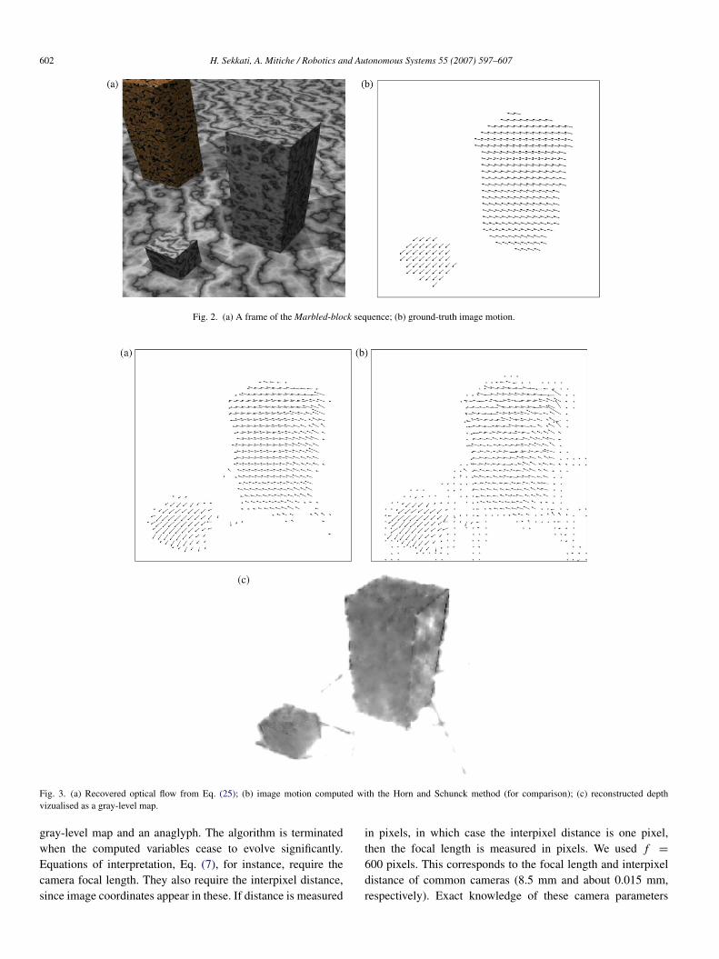
Fig. 3. (a) Recovered optical flow from Eq. (25); (b) image motion computed with the Horn and Schunck method (for comparison); (c) reconstructed depthvizualised as a gray-level map.

gray-level map and an anaglyph. The algorithm is terminatedwhen the computed variables cease to evolve significantly.Equations of interpretation, Eq. (7), for instance, require thecamera focal length. They also require the interpixel distance,since image coordinates appear in these. If distance is measured

in pixels, in which case the interpixel distance is one pixel,then the focal length is measured in pixels. We used f =

600 pixels. This corresponds to the focal length and interpixeldistance of common cameras (8.5 mm and about 0.015 mm,respectively). Exact knowledge of these camera parameters


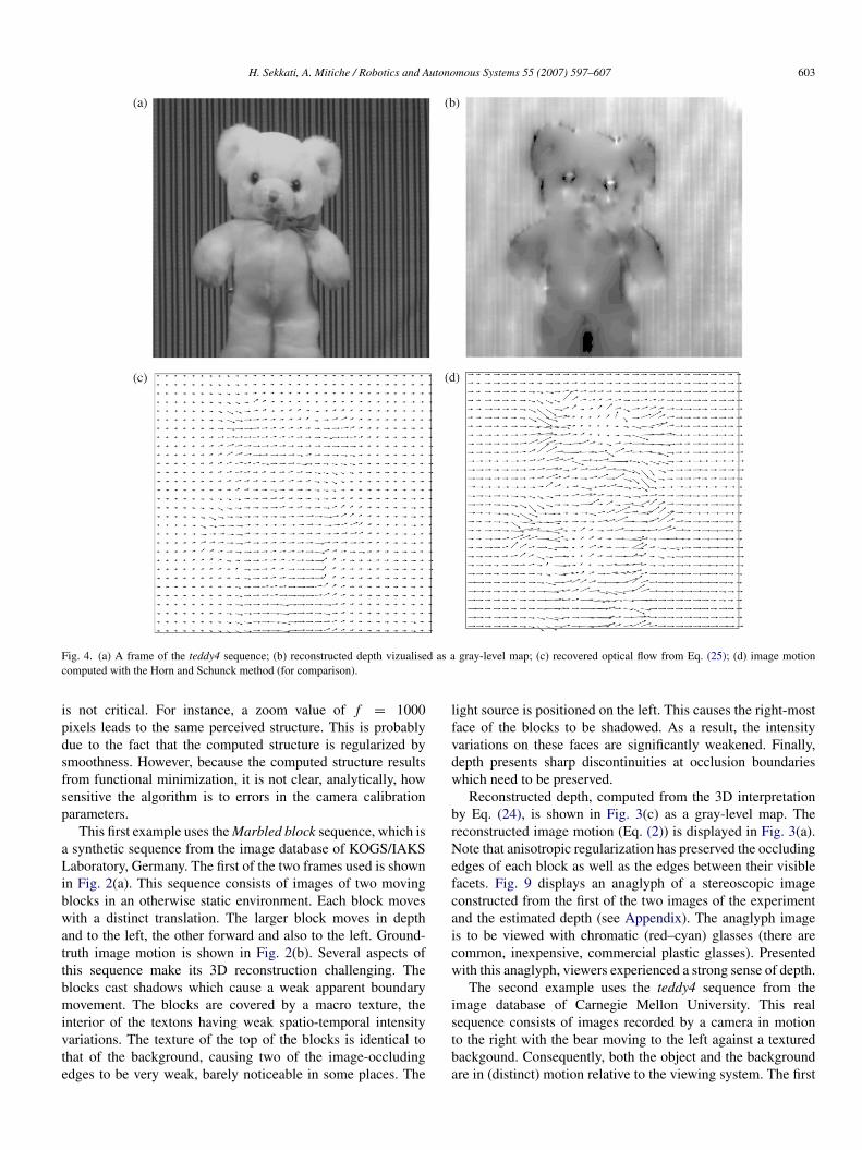
Fig. 4. (a) A frame of the teddy4 sequence; (b) reconstructed depth vizualised as a gray-level map; (c) recovered optical flow from Eq. (25); (d) image motioncomputed with the Horn and Schunck method (for comparison).

is not critical. For instance, a zoom value of f = 1000pixels leads to the same perceived structure. This is probablydue to the fact that the computed structure is regularized bysmoothness. However, because the computed structure resultsfrom functional minimization, it is not clear, analytically, howsensitive the algorithm is to errors in the camera calibrationparameters.

This first example uses the Marbled block sequence, which isa synthetic sequence from the image database of KOGS/IAKSLaboratory, Germany. The first of the two frames used is shownin Fig. 2(a). This sequence consists of images of two movingblocks in an otherwise static environment. Each block moveswith a distinct translation. The larger block moves in depthand to the left, the other forward and also to the left. Ground-truth image motion is shown in Fig. 2(b). Several aspects ofthis sequence make its 3D reconstruction challenging. Theblocks cast shadows which cause a weak apparent boundarymovement. The blocks are covered by a macro texture, theinterior of the textons having weak spatio-temporal intensityvariations. The texture of the top of the blocks is identical tothat of the background, causing two of the image-occludingedges to be very weak, barely noticeable in some places. The

light source is positioned on the left. This causes the right-mostface of the blocks to be shadowed. As a result, the intensityvariations on these faces are significantly weakened. Finally,depth presents sharp discontinuities at occlusion boundarieswhich need to be preserved.

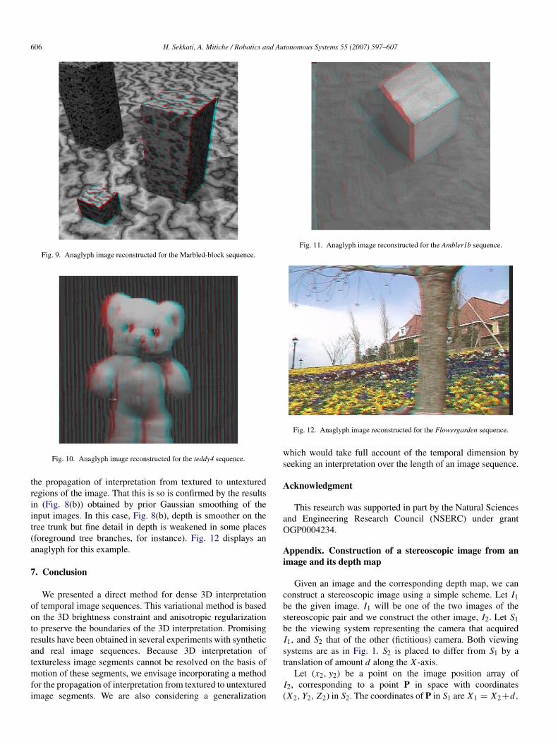
Reconstructed depth, computed from the 3D interpretationby Eq. (24), is shown in Fig. 3(c) as a gray-level map. Thereconstructed image motion (Eq. (2)) is displayed in Fig. 3(a).Note that anisotropic regularization has preserved the occludingedges of each block as well as the edges between their visiblefacets. Fig. 9 displays an anaglyph of a stereoscopic imageconstructed from the first of the two images of the experimentand the estimated depth (see Appendix). The anaglyph imageis to be viewed with chromatic (red–cyan) glasses (there arecommon, inexpensive, commercial plastic glasses). Presentedwith this anaglyph, viewers experienced a strong sense of depth.

The second example uses the teddy4 sequence from theimage database of Carnegie Mellon University. This realsequence consists of images recorded by a camera in motionto the right with the bear moving to the left against a texturedbackgound. Consequently, both the object and the backgroundare in (distinct) motion relative to the viewing system. The first


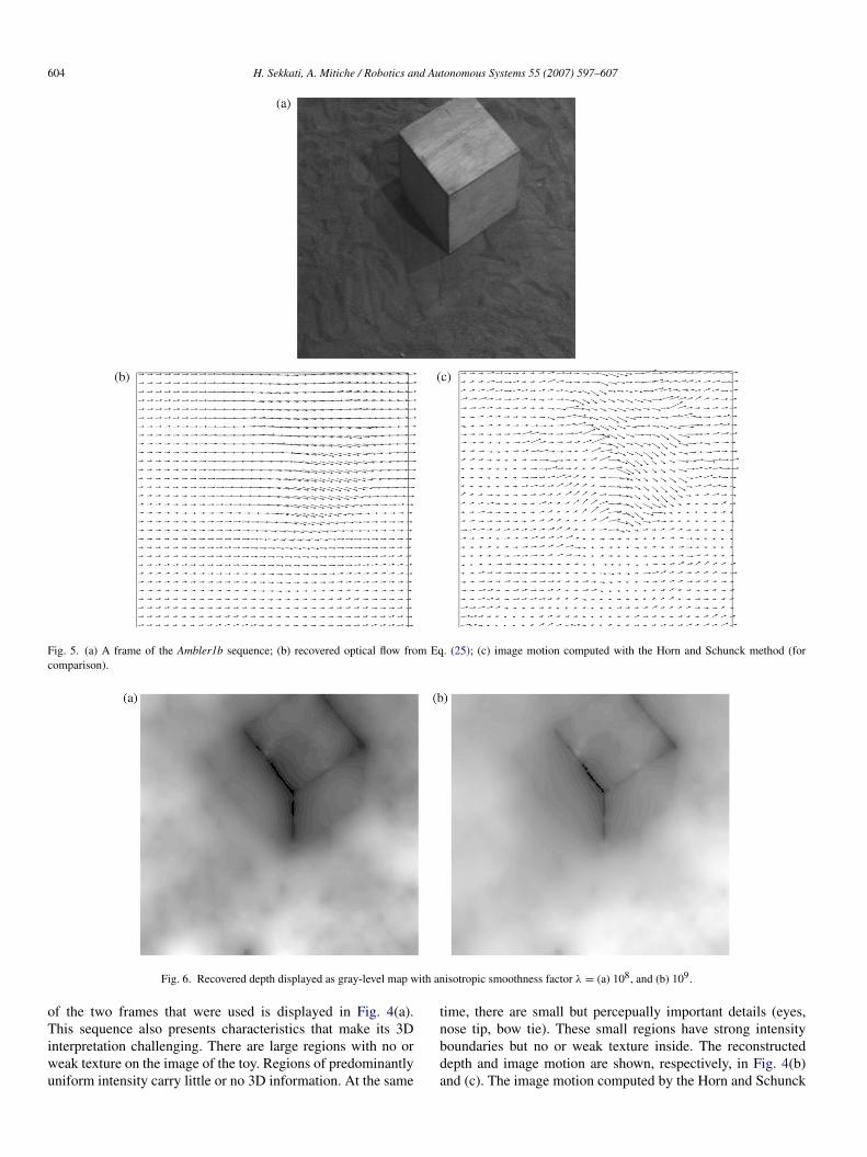
Fig. 5. (a) A frame of the Ambler1b sequence; (b) recovered optical flow from Eq. (25); (c) image motion computed with the Horn and Schunck method (forcomparison).

Fig. 6. Recovered depth displayed as gray-level map with anisotropic smoothness factor λ = (a) 108, and (b) 109.

of the two frames that were used is displayed in Fig. 4(a).This sequence also presents characteristics that make its 3Dinterpretation challenging. There are large regions with no orweak texture on the image of the toy. Regions of predominantlyuniform intensity carry little or no 3D information. At the same

time, there are small but percepually important details (eyes,nose tip, bow tie). These small regions have strong intensityboundaries but no or weak texture inside. The reconstructeddepth and image motion are shown, respectively, in Fig. 4(b)and (c). The image motion computed by the Horn and Schunck


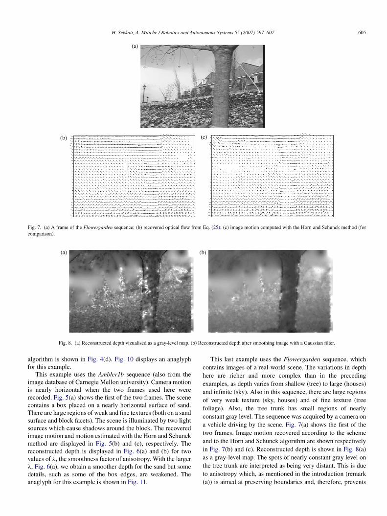
Fig. 7. (a) A frame of the Flowergarden sequence; (b) recovered optical flow from Eq. (25); (c) image motion computed with the Horn and Schunck method (forcomparison).

Fig. 8. (a) Reconstructed depth vizualised as a gray-level map. (b) Reconstructed depth after smoothing image with a Gaussian filter.

algorithm is shown in Fig. 4(d). Fig. 10 displays an anaglyphfor this example.

This example uses the Ambler1b sequence (also from theimage database of Carnegie Mellon university). Camera motionis nearly horizontal when the two frames used here wererecorded. Fig. 5(a) shows the first of the two frames. The scenecontains a box placed on a nearly horizontal surface of sand.There are large regions of weak and fine textures (both on a sandsurface and block facets). The scene is illuminated by two lightsources which cause shadows around the block. The recoveredimage motion and motion estimated with the Horn and Schunckmethod are displayed in Fig. 5(b) and (c), respectively. Thereconstructed depth is displayed in Fig. 6(a) and (b) for twovalues of λ, the smoothness factor of anisotropy. With the largerλ, Fig. 6(a), we obtain a smoother depth for the sand but somedetails, such as some of the box edges, are weakened. Theanaglyph for this example is shown in Fig. 11.

This last example uses the Flowergarden sequence, whichcontains images of a real-world scene. The variations in depthhere are richer and more complex than in the precedingexamples, as depth varies from shallow (tree) to large (houses)and infinite (sky). Also in this sequence, there are large regionsof very weak texture (sky, houses) and of fine texture (treefoliage). Also, the tree trunk has small regions of nearlyconstant gray level. The sequence was acquired by a camera ona vehicle driving by the scene. Fig. 7(a) shows the first of thetwo frames. Image motion recovered according to the schemeand to the Horn and Schunck algorithm are shown respectivelyin Fig. 7(b) and (c). Reconstructed depth is shown in Fig. 8(a)as a gray-level map. The spots of nearly constant gray level onthe tree trunk are interpreted as being very distant. This is dueto anisotropy which, as mentioned in the introduction (remark(a)) is aimed at preserving boundaries and, therefore, prevents


Fig. 9. Anaglyph image reconstructed for the Marbled-block sequence.

Fig. 10. Anaglyph image reconstructed for the teddy4 sequence.

the propagation of interpretation from textured to untexturedregions of the image. That this is so is confirmed by the resultsin (Fig. 8(b)) obtained by prior Gaussian smoothing of theinput images. In this case, Fig. 8(b), depth is smoother on thetree trunk but fine detail in depth is weakened in some places(foreground tree branches, for instance). Fig. 12 displays ananaglyph for this example.

7. Conclusion

We presented a direct method for dense 3D interpretationof temporal image sequences. This variational method is basedon the 3D brightness constraint and anisotropic regularizationto preserve the boundaries of the 3D interpretation. Promisingresults have been obtained in several experiments with syntheticand real image sequences. Because 3D interpretation oftextureless image segments cannot be resolved on the basis ofmotion of these segments, we envisage incorporating a methodfor the propagation of interpretation from textured to untexturedimage segments. We are also considering a generalization

Fig. 11. Anaglyph image reconstructed for the Ambler1b sequence.

Fig. 12. Anaglyph image reconstructed for the Flowergarden sequence.

which would take full account of the temporal dimension byseeking an interpretation over the length of an image sequence.

Acknowledgment

This research was supported in part by the Natural Sciencesand Engineering Research Council (NSERC) under grantOGP0004234.

Appendix. Construction of a stereoscopic image from animage and its depth map

Given an image and the corresponding depth map, we canconstruct a stereoscopic image using a simple scheme. Let I1be the given image. I1 will be one of the two images of thestereoscopic pair and we construct the other image, I2. Let S1be the viewing system representing the camera that acquiredI1, and S2 that of the other (fictitious) camera. Both viewingsystems are as in Fig. 1. S2 is placed to differ from S1 by atranslation of amount d along the X -axis.

Let (x2, y2) be a point on the image position array ofI2, corresponding to a point P in space with coordinates(X2, Y2, Z2) in S2. The coordinates of P in S1 are X1 = X2+d,


Y1 = Y2, and Z2 = Z1. The image of P in the image domain ofI1 are, according to our viewing system model (Fig. 1):

x1 = fX1

Z1(26)

y1 = y2. (27)

Because depth has been estimated, coordinates (x1, y1) areknown. Image I2, which will be the second of the stereoscopicpair, is then constructed as follows:

I2(x2, y2) = I1(x1, y1) (28)

where x1 is the x-coordinate of the point on the image positionalarray of I1 with x coordinate closest to x1. Alternatively, onecan use interpolation. However, we found it unnecessary forour purpose here.

References

[1] J. Aggarwal, N. Nandhakumar, On the computation of motion from asequence of images: A review, Proceedings of the IEEE 76 (8) (1988)917–935.

[2] T. Huang, A. Netravali, Motion and structure from feature correspon-dences: A review, Proceedings of the IEEE 82 (2) (1994) 252–268.

[3] O. Faugeras, Three Dimensional Computer Vision: A Geometric Viewpoint, MIT Press, Cambridge, MA, 1993.

[4] A. Mitiche, Computational Analysis of Visual Motion, Plenum Press,New York, 1994.

[5] A. Zisserman, R. Hartley, Multiple View Geometry in Computer Vision,Cambridge University Press, Cambridge, MA, 2000.

[6] B. Horn, B. Schunk, Determining optical flow, Artificial Intelligence 17(1–3) (1981) 185–203.

[7] G. Aubert, R. Deriche, P. Kornprobst, Computing optical flow viavariational thechniques, SIAM Journal of Applied Mathematics 60 (1)(1999) 156–182.

[8] A. Mitiche, P. Bouthemy, Computation and analysis of image motion:A synopsis of current problems and methods, International Journal ofComputer Vision 19 (1) (1996) 29–55.

[9] J. Mellor, S. Teller, T. Lozano-Perez, Dense depth map from epipolarimages, in: DARPA Image Understanding Workshop, 1997, pp. 893–900.

[10] Z. Marco, J. Victor, H. Christensen, Constrained structure and motionestimation from optical flow, in: International Conference on PatternRecognition, vol. 1, Quebec, 2002, pp. 339–342.

[11] H. Sekkati, A. Mitiche, Joint dense 3D interpretation and multiple motionsegmentation of temporal image sequences: A variational framework withactive curve evolution and level sets, in: International Conference onImage Processing, Singapore, 2004, pp. 549–552.

[12] A. Mitiche, S. Hadjres, MDL estimation of a dense map of relative depthand 3D motion from a temporal sequence of images, Pattern Analysis andApplications (6) (2003) 78–87.

[13] G. Adiv, Determining three-dimensional motion and structure fromoptical flow generated by several moving objects, IEEE Transactions onPattern Analysis and Machine Intelligence 7 (4) (1985) 384–401.

[14] S. Negahdaripour, B. Horn, Direct passive navigation, IEEE Transactionson Pattern Analysis and Machine Intelligence 9 (1) (1987) 168–176.

[15] B. Horn, E. Weldon, Direct methods for recovering motion, InternationalJournal of Computer Vision 2 (2) (1988) 51–76.

[16] R. Laganiere, A. Mitiche, Direct Bayesian interpretation of visual motion,Journal of Robotics and Autonomous Systems 14 (4) (1995) 247–254.

[17] R. Chellappa, S. Srinivasan, Structure from motion: Sparse versus

dense correspondance methods, in: International Conference on ImageProcessing, vol. 2, Kobe, Japan, 1999, pp. 492–499.

[18] Y. Hung, H. Ho, A Kalman filter approach to direct depth estimationincorporating surface structure, IEEE Transactions on Pattern Analysisand Machine Intelligence 21 (6) (1999) 570–575.

[19] S. Stein, M. Shashua, Model-based brightness constraints: On directestimation of structure and motion, IEEE Transactions on Pattern Analysisand Machine Intelligence 22 (9) (2000) 993–1005.

[20] S. Srinivasan, Extracting structure from optical flow using the fast errorsearch technique, International Journal of Computer Vision 37 (3) (2000)203–230.

[21] T. Brodsky, C. Fermuller, Y. Aloimonos, Structure from motion: Beyondthe epipolar constraint, International Journal of Computer Vision 37 (3)(2000) 231–258.

[22] F. Martinez, J. Benois-Pineau, D. Barda, Extraction of the relative depthinformation of objects in video sequences, in: International Conference onImage Precessing, Chicago, IL, 1998, pp. 948–952.

[23] F. Morier, H. Nicolas, J. Benois, D. Barda, H. Hanson, Relative depthestimation of video objects for image interpolation, in: InternationalConference on Image Precessing, 1998, pp. 953–957.

[24] J. Rissanen, Modeling by shortest data description, Automatica 14 (1978)465–471.

[25] Y. Leclerc, Constructing simple stable descriptions for image partitioning,International Journal of Computer Vision 3 (1) (1996) 73–102.

[26] H. Sekkati, A. Mitiche, Dense 3D interpretation of image sequences:A variational approach using anisotropic diffusion, in: InternationalConference on Image Analysis and Processing, Mantova, Italy, 2003.

[27] H. Longuet-Higgins, K. Prazdny, The interpretation of a moving retinalimage, Proceedings of the Royal Society of London, Series B 208 (1981)385–397.

[28] D. Geman, G. Reynolds, Constrained restoration and the recovery ofdiscontinuities, IEEE Transactions on Pattern Analysis and MachineIntelligence 14 (3) (1993) 367–383.

[29] P. Perona, J. Malik, Scale space and edge detection using anisotropicdiffusion, IEEE Transactions on Pattern Analysis and MachineIntelligence 12 (7) (1981) 629–639.

[30] P. Ciarlet, Introduction a l’analyse numerique matricielle et al’ optimisation, fifth ed., Masson, Paris, 1994.

[31] E. Dubois, A projection method to generate anaglyph stereo images,in: Proc. International Conference on Acoustics, Speech, and SignalProcessing, vol. III, Salt Lake City, USA, 2001, pp. 1661–1664.

Dr. Hicham Sekkati received the M.Sc. and Ph.D.degrees in 2003 and 2005 from the Institut Nationalde la Recherche Scientifique (INRS-EMT), Montreal,Canada. The subject of his Ph.D. thesis was variationalsegmentation and 3D interpretation of monocularimage sequences. In 2005, he joined the ComputerVision Laboratory at the University of Miami, FL, asa postdoctoral associate, pursuing research on opti-acoustic image processing for underwater applications.

Prof. Amar Mitiche holds a Licence Es Sciencesin mathematics from the University of Algiers anda Ph.D. in computer science from the Universityof Texas at Austin. He is currently a professorat the Institut National de Recherche Scientifique(INRS), department of telecommunications (INRS-EMT), in Montreal, Quebec, Canada. His researchis in computer vision. His current interests includeimage segmentation, motion analysis in monocular and

stereoscopic image sequences (detection, estimation, segmentation, tracking,3D interpretation) with a focus on level set methods, and written textrecognition with a focus on neural networks methods.

A variational method for the recovery of dense 3D structure from motion

Documents

Transcript of A variational method for the recovery of dense 3D structure from motion