Linear Algebra and its Applications 418 (2006) 551–564www.elsevier.com/locate/laa

A variant of Jensen’s inequality of Mercer’s typefor operators with applications

A. Matkovic a, J. Pecaric b ,∗, I. Peric c

a Department of Mathematics, Faculty of Natural Sciences, Mathematics and Education,University of Split, Teslina 12, 21000 Split, Croatia

b Faculty of Textile Technology, University of Zagreb, Pierottijeva 6, 10000 Zagreb, Croatiac Faculty of Food Technology and Biotechnology, University of Zagreb, Pierottijeva 6,

10000 Zagreb, Croatia

Received 24 October 2005; accepted 28 February 2006Available online 2 May 2006Submitted by R.A. Brualdi

Abstract

A variant of Jensen’s operator inequality for convex functions, which is a generalization of Mercer’sresult, is proved. Obtained result is used to prove a monotonicity property for Mercer’s power means foroperators, and a comparison theorem for quasi-arithmetic means for operators.© 2006 Elsevier Inc. All rights reserved.

AMS classification: 47A63; 47A64

Keywords: Jensen’s operator inequality; Monotonicity; Power means; Quasi-arithmetic means

1. Introduction

For a given a < b, let x = (x1, . . . , xk) be such that a � x1 � x2 � · · · � xk � b and w =(w1, . . . , wk) be nonnegative weights such that

∑kj=1wj = 1. Mercer [3] proved the following

variant of Jensen’s inequality.

∗ Corresponding author.E-mail addresses: anita@pmfst.hr (A. Matkovic), pecaric@hazu.hr (J. Pecaric), iperic@pbf.hr (I. Peric).

0024-3795/$ - see front matter ( 2006 Elsevier Inc. All rights reserved.doi:10.1016/j.laa.2006.02.030

552 A. Matkovic et al. / Linear Algebra and its Applications 418 (2006) 551–564

Theorem A. If f is a convex function on [a, b] then

f

a + b −k∑j=1

wjxj

� f (a)+ f (b)−k∑j=1

wjf (xj ).

For a > 0 the (weighted) power means Mr(x,w) are defined as

Mr(x,w) =

(k∑j=1

wjxrj

) 1r

, r /= 0,

exp

(k∑j=1

wj ln xj

), r = 0.

In [4] Mercer defined the family of functions

Qr(a, b, x) =[ar + br −Mr

r (x,w)] 1r , r /= 0,

ab

M0(x,w), r = 0

and proved the following.

Theorem B. For r < s, Qr(a, b, x) � Qs(a, b, x).

In this paper we consider similar inequalities in a more general setting. To do this we needsome well known results. The first one is Löwner–Heinz inequality (see for example [5, p. 9]).

Theorem C. Let A and B be positive operators on a Hilbert space H. If A � B, then Ap � Bp

for all p ∈ [0, 1].

In [5, p. 220, 232, 250] the following theorems are also proved.

Theorem D. Let A,B be positive operators on a Hilbert space H with Sp(A) ⊆ [m1,M1], andSp(B) ⊆ [m2,M2] for some scalars Mj > mj > 0 (j = 1, 2). If A � B, then the followinginequalities hold:

(i) for all p > 1:K(m1,M1, p)A

p � Bp,

K(m2,M2, p)Ap � Bp,

(ii) for all p < −1:K(m1,M1, p)B

p � Ap,

K(m2,M2, p)Bp � Ap,

where a generalized Kantorovich constant K(m,M,p) is defined by

K(m,M,p) = (mMp −Mmp)

(p − 1)(M −m)

(p − 1

p

Mp −mp

mMp −Mmp

)pfor all p ∈ R.

A. Matkovic et al. / Linear Algebra and its Applications 418 (2006) 551–564 553

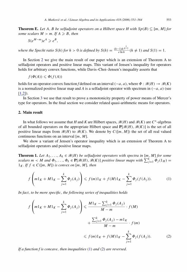
Theorem E. Let A,B be selfadjoint operators on a Hilbert space H with Sp(B) ⊆ [m,M] forsome scalars M > m. If A � B, then

S(eM−m)eA � eB,

where the Specht ratio S(h) for h > 0 is defined by S(h) = (h−1)h1h−1

e ln h (h /= 1) and S(1) = 1.

In Section 2 we give the main result of our paper which is an extension of Theorem A toselfadjoint operators and positive linear maps. This variant of Jensen’s inequality for operatorsholds for arbitrary convex functions, while Davis–Choi–Jensen’s inequality asserts that

f (�(A)) � �(f (A))

holds for an operator convex function f defined on an interval (−a, a), where � : B(H) → B(K)is a normalized positive linear map and A is a selfadjoint operator with spectrum in (−a, a) (see[1,2]).

In Section 3 we use that result to prove a monotonicity property of power means of Mercer’stype for operators. In the final section we consider related quasi-arithmetic means for operators.

2. Main result

In what follows we assume that H and K are Hilbert spaces, B(H) and B(K) are C∗-algebrasof all bounded operators on the appropriate Hilbert space and P[B(H),B(K)] is the set of allpositive linear maps from B(H) to B(K). We denote by C([m,M]) the set of all real valuedcontinuous functions on an interval [m,M].

We show a variant of Jensen’s operator inequality which is an extension of Theorem A toselfadjoint operators and positive linear maps.

Theorem 1. Let A1, . . ., Ak ∈ B(H) be selfadjoint operators with spectra in [m,M] for somescalars m < M and �1, . . .,�k ∈ P[B(H),B(K)] positive linear maps with

∑kj=1 �j (1H ) =

1K. If f ∈ C([m,M]) is convex on [m,M], then

f

m1K +M1K −k∑j=1

�j (Aj )

� f (m)1K + f (M)1K −k∑j=1

�j (f (Aj )). (1)

In fact, to be more specific, the following series of inequalities holds

f

m1K +M1K −k∑j=1

�j (Aj )

�M1K −∑k

j=1 �j (Aj )

M −m· f (M)

+∑kj=1 �j (Aj )−m1K

M −m· f (m)

� f (m)1K + f (M)1K −k∑j=1

�j (f (Aj )). (2)

If a function f is concave, then inequalities (1) and (2) are reversed.

554 A. Matkovic et al. / Linear Algebra and its Applications 418 (2006) 551–564

Proof. Since f is continuous and convex, the same is also true for the function g : [m,M] → Rdefined by g(t) = f (m+M − t), t ∈ [m,M]. Hence, the following inequalities hold for everyt ∈ [m,M] (see for example [6, p. 2]):

f (t) � t −m

M −m· f (M)+ M − t

M −m· f (m),

g(t) � t −m

M −m· g(M)+ M − t

M −m· g(m).

Since m1H � Aj � M1H for j = 1, . . . , k and∑kj=1 �j (1H ) = 1K , it follows that m1K �∑k

j=1 �j (Aj ) � M1K . Now, using the functional calculus we have

g

k∑j=1

�j (Aj )

�∑kj=1 �j (Aj )−m1K

M −m· g(M)+ M1K −∑k

j=1 �j (Aj )

M −m· g(m)

or

f

m1K +M1K −k∑j=1

�j (Aj )

�∑kj=1 �j (Aj )−m1K

M −m· f (m)+ M1K −∑k

j=1 �j (Aj )

M −m· f (M)

= f (m)1K + f (M)1K

−[M1K −∑k

j=1 �j (Aj )

M −m· f (m)+

∑kj=1 �j (Aj )−m1K

M −m· f (M)

]. (3)

On the other hand, using the functional calculus we also have

f (Aj ) � Aj −m1HM −m

· f (M)+ M1H − Aj

M −m· f (m).

Applying positive linear maps �j and summing, it follows that

k∑j=1

�j (f (Aj ))�∑kj=1 �j (Aj )−m1K

M −m· f (M)+M1K −∑k

j=1 �j (Aj )

M −m· f (m). (4)

Using inequalities (3) and (4), we obtain desired inequalities (1) and (2).The last statement follows immediately from the fact that ifϕ is concave then −ϕ is convex. �

3. Applications to Mercer’s power means

We suppose that:

(i) A = (A1, . . . , Ak), where Aj ∈ B(H) are positive invertible operators with Sp(Aj ) ⊆[m,M] for some scalars 0 < m < M .

(ii) � = (�1, . . . ,�k), where �j ∈ P[B(H), B(K)] are positive linear maps with∑kj=1 �j (1H ) = 1K .

A. Matkovic et al. / Linear Algebra and its Applications 418 (2006) 551–564 555

(iii) �(m,M,p) = K(mp,Mp, 1p) = p(mpM−Mpm)

(1−p)(Mp−mp)((1−p)(M−m)mpM−Mpm

) 1p

, for 0 < m < M

and p ∈ R, p /= 0. Set: �(m,M, 0) = limp→0 �(m,M,p) = S(Mm

) = M−mlnM−lnm

exp(m(1+lnM)−M(1+lnm)

M−m)

.

We define, for any r ∈ R

Mr(A,�) :=

[mr1K +Mr1K −

k∑j=1

�j (Arj )]1r , r /= 0,

exp

((lnm)1K + (lnM)1K −

k∑j=1

�j (ln(Aj ))

), r = 0.

Observe that, since 0 < m1H � Aj � M1H , it follows that:

• 0 < mr1H � Arj � Mr1H holds for all r > 0,• 0 < Mr1H � Arj � mr1H holds for all r < 0,• (lnm)1H � ln(Aj ) � (lnM)1H (j = 1, . . . , k).

Applying positive linear maps �j and summing, it follows that:

• 0 < mr1K �∑kj=1 �j (Arj ) � Mr1K , for all r > 0,

• 0 < Mr1K �∑kj=1 �j (Arj ) � mr1K , for all r < 0,

• (lnm)1K �∑kj=1 �j (ln(Aj )) � (lnM)1K ,

since∑kj=1 �j (1H ) = 1K . Hence, Mr(A,�) is well defined.

Furthermore, we define, for any r, s ∈ R

S(r, s,A,�) :=

[Mr1K−SrMr−mr ·Ms + Sr−mr1K

Mr−mr ·ms] 1s, r /= 0, s /= 0,

exp(Mr1K−SrMr−mr · lnM + Sr−mr1K

Mr−mr · lnm), r /= 0, s = 0,[

(lnM)1K−S0lnM−lnm ·Ms + S0−(lnm)1K

lnM−lnm ·ms] 1s, r = 0, s /= 0,

where Sr = ∑kj=1 �j (Arj ) and S0 = ∑k

j=1 �j (ln(Aj )). It is easy to see that S(r, s,A,�) is alsowell defined.

Theorem 2. Let r, s ∈ R, r < s.

(i) If either r � −1 or s � 1, then

Mr(A,�) � Ms(A,�).

(ii) If −1 < r and s < 1, then

Mr(A,�) � �(m,M, s) · Ms(A,�).

Proof. (i) Step 1: Suppose that 0 < r < s and s � 1.Applying the inequality (1) to the convex function f (t) = t

sr (note that s

r> 1 here) and

replacing Aj , m and M with Arj , mr and Mr , respectively, we have

556 A. Matkovic et al. / Linear Algebra and its Applications 418 (2006) 551–564

mr1K +Mr1K −k∑j=1

�j (Arj )

sr

� ms1K +Ms1K −k∑j=1

�j (Asj ). (5)

Raising both sides to the power 1s(0 < 1

s� 1), it follows from Theorem C that

Mr(A,�) � Ms(A,�).

Step 2: Suppose that r < 0 and s � 1.Applying the inequality (1) to the convex function f (t) = t

sr (note that s

r< 0 here) and

proceeding in the same way as in Step 1, we have

Mr(A,�) � Ms(A,�).

Step 3: Suppose that r = 0 and s � 1.Applying the inequality (1) to the convex function f (t) = exp(s · t) and replacing Aj , m and

M with ln(Aj ), lnm and lnM , respectively, we have

exp

s(lnm)1K + (lnM)1K −

k∑j=1

�j (ln(Aj ))

� exp(s lnm)1K + exp(s lnM)1K −

k∑j=1

�j (exp(s ln(Aj )))

= ms1K +Ms1K −k∑j=1

�j (Asj ) (6)

or

[M0(A,�)]s � [Ms(A,�)]s .Raising both sides to the power 1

s(0 < 1

s� 1), it follows from Theorem C that

M0(A,�) � Ms(A,�).

Step 4: Suppose that r < s < 0 and r � −1.Applying the inequality (1) to the convex function f (t) = t

rs (note that r

s> 1 here) and

replacing Aj , m and M with Asj , ms and Ms , respectively, we havems1K +Ms1K −k∑j=1

�j (Asj ))

rs

� mr1K +Mr1K −k∑j=1

�j (Arj ). (7)

Raising both sides to the power − 1r(0 < − 1

r� 1), it follows from Theorem C that

[Ms(A,�)]−1 � [Mr(A,�)]−1.

Hence, we have

Mr(A,�) � Ms(A,�).

Step 5: Suppose that s > 0 and r � −1.

A. Matkovic et al. / Linear Algebra and its Applications 418 (2006) 551–564 557

Applying the inequality (1) to the convex function f (t) = trs (note that r

s< 0 here) and

proceeding in the same way as in Step 4, we have

Mr(A,�) � Ms(A,�).

Step 6: Suppose that s = 0 and r � −1.Applying the inequality (1) to the convex function f (t) = exp(r · t) and replacing Aj , m and

M with ln(Aj ), lnm and lnM , respectively, we have

exp

r(lnm)1K + (lnM) 1K −

k∑j=1

�j (ln(Aj ))

� exp(r lnm)1K + exp(r lnM)1K −

k∑j=1

�j (exp(r ln(Aj )))

= mr1K +Mr1K −k∑j=1

�j (Arj ) (8)

or

[M0(A,�)]r � [Mr(A,�)]r .Raising both sides to the power − 1

r(0 < 1

r� 1), it follows from Theorem C that

[M0(A,�)]−1 � [Mr(A,�)]−1.

Hence, we have

Mr(A,�) � M0(A,�).

(ii) Step 1: Suppose that 0 < r < s < 1.In the same way as in (i) Step 1 we obtain inequality (5). Observe that, since ms1K �∑kj=1 �j (Asj ) � Ms1K , it follows thatms1K � ms1K +Ms1K −∑k

j=1 �j (Asj ) � Ms1K . Rais-

ing both sides of (5) to the power 1s( 1s> 1), it follows from Theorem D (i) that

Mr(A,�) � K

(ms,Ms,

1

s

)Ms(A,�).

Step 2: Suppose that 0 = r < s < 1.In the same way as in (i) Step 3 we obtain inequality (6). With the same observation as in (ii)

Step 1 and raising both sides of (6) to the power 1s( 1s> 1), it follows from Theorem D (i) that

M0(A,�) � K

(ms,Ms,

1

s

)Ms(A,�).

Step 3: Suppose that −1 < r < s < 0.Applying reversed inequality (1) to the concave function f (t) = t

sr (note that 0 < s

r< 1 here)

and replacing Aj , m and M with Arj , mr and Mr , respectively, we obtain reversed inequality (5).

Observe that, sinceMs1K �∑kj=1 �j (Asj ) � ms1K , it follows thatMs1K � ms1K +Ms1K −∑k

j=1 �j (Asj ) � ms1K . Raising both sides of reversed (5) to the power 1s( 1s< −1), it follows

from Theorem D (ii) that

558 A. Matkovic et al. / Linear Algebra and its Applications 418 (2006) 551–564

Mr(A,�) � K

(Ms,ms,

1

s

)Ms(A,�).

Since K(M,m, p) = K(m,M,p) (see [5, p. 77]), we have

Mr(A,�) � K

(ms,Ms,

1

s

)Ms(A,�).

Step 4: Suppose that −1 < r < s = 0.Applying the inequality (1) to the convex function f (t) = 1

rln t and replacing Aj , m and M

with Arj , Mr and mr , respectively, we obtain

1

rln

mr1K +Mr1K −k∑j=1

�j (Arj )

� (lnm)1K + (lnM)1K −k∑j=1

�j (ln(Aj ).

Observing that both sides have spectra in [lnm, lnM], it follows from Theorem E that

Mr(A,�) � �(m,M, 0)M0(A,�).

Step 5: Suppose that −1 < r < 0 < s < 1.In the same way as in (i) Step 2 we obtain inequality (5). With the same observation as in (ii)

Step 1 and raising both sides of (5) to the power 1s( 1s> 1), it follows from Theorem D (i) that

Mr(A,�) � K

(ms,Ms,

1

s

)Ms(A,�). �

If we use inequalities (2) instead of the inequality (1), then we have the following results:

Theorem 3. Let r, s ∈ R, r < s.

(i) If s � 1, then

Mr(A,�) � S(r, s,A,�) � Ms(A,�).

If r � −1, then

Mr(A,�) � S(s, r,A,�) � Ms(A,�).

(ii) If −1 < r and s < 1, then

1

�(m,M, s)· Mr(A,�) � S(r, s,A,�) � �(m,M, s) · Ms(A,�).

Proof. (i) Step 1: Suppose that 0 < r < s and s � 1.Applying inequalities (2) to the convex functionf (t) = t

sr (note that s

r� 1 here) and replacing

Aj , m and M with Arj , mr and Mr , respectively, we havemr1K +Mr1K −k∑j=1

�j (Arj )

sr

� Mr1K − Sr

Mr −mr·Ms + Sr −mr1K

Mr −mr·ms

� ms1K +Ms1K −k∑j=1

�j (Asj ). (9)

A. Matkovic et al. / Linear Algebra and its Applications 418 (2006) 551–564 559

Raising these inequalities to the power 1s(0 < 1

s� 1), it follows from Theorem C that

Mr(A,�) � S(r, s,A,�) � Ms(A,�).

Step 2: Suppose that r < 0 and s � 1.Applying inequalities (2) to the convex function f (t) = t

sr (note that s

r< 0 here) and pro-

ceeding in the same way as in Step 1, we have

Mr(A,�) � S(r, s,A,�) � Ms(A,�).

Step 3: Suppose that r = 0 and s � 1.Applying inequalities (2) to the convex function f (t) = exp(s · t) and replacing Aj , m and M

with ln(Aj ), lnm and lnM , respectively, we have

exp

s(lnm)1K + (lnM)1K −

k∑j=1

�j (ln(Aj ))

� (lnM)1K − S0

lnM − lnm· exp(s lnM)+ S0 − (lnm)1K

lnM − lnm· exp(s lnm)

� exp(s lnm)1K + exp(s lnM)1K −k∑j=1

�j (exp(s ln(Aj )))

= ms1K +Ms1K −k∑j=1

�j (Asj ) (10)

or

[M0(A,�)]s � [S(0, s,A,�)]s � [Ms(A,�)]s .Raising these inequalities to the power 1

s(0 < 1

s� 1), it follows from Theorem C that

M0(A,�) � S(0, s,A,�) � Ms(A,�).

Step 4: Suppose that r < s < 0 and r � −1.Applying inequalities (2) to the convex functionf (t) = t

rs (note that r

s� 1 here) and replacing

Aj , m and M with Asj , ms and Ms , respectively, we havems1K +Ms1K −k∑j=1

�j (Asj )

rs

� Ms1K − Sr

Ms −ms·Mr + Sr −ms1K

Ms −ms·mr

� mr1K +Mr1K −k∑j=1

�j (Arj ).

Raising these inequalities to the power − 1r(0 < − 1

r� 1), it follows from Theorem C that

[Ms(A,�)]−1 � [S(s, r,A,�)]−1 � [Mr(A,�)]−1.

Hence, we have

Mr(A,�) � S(s, r,A,�) � Ms(A,�).

560 A. Matkovic et al. / Linear Algebra and its Applications 418 (2006) 551–564

Step 5: Suppose that s > 0 and r � −1.Applying inequalities (2) to the convex function f (t) = t

rs (note that r

s< 0 here) and pro-

ceeding in the same way as in Step 4, we have

Mr(A,�) � S(s, r,A,�) � Ms(A,�).

Step 6: Suppose that s = 0 and r � −1.Applying inequalities (2) to the convex function f (t) = exp(r · t) and replacing Aj , m and M

with ln(Aj ), lnm and lnM , respectively, we have

exp

r(lnm)1K + (lnM)1K −

k∑j=1

�j (ln(Aj ))

� (lnM)1K − S0

lnM − lnm· exp(r lnM)+ S0 − (lnm)1K

lnM − lnm· exp(r lnm)

� exp(r lnm)1K + exp(r lnM)1K −k∑j=1

�j (exp(r ln(Aj )))

= mr1K +Mr1K −k∑j=1

�j (Arj )

or

[M0(A,�)]r � [S(0, r,A,�)]r � [Mr(A,�)]r .Raising these inequalities to the power − 1

r(0 < 1

r� 1), it follows from Theorem C that

[M0(A,�)]−1 � [S(0, r,A,�)]−1 � [Mr(A,�)]−1.

Hence, we have

Mr(A,�) � S(0, r,A,�) � M0(A,�).

(ii) Step 1: Suppose that 0 < r < s < 1.In the same way as in (i) Step 1 we obtain inequalities (9). Observe that, since mr1K �∑kj=1 �j (Arj ) � Mr1K andms1K �

∑kj=1 �j (Asj ) � Ms1K , it follows thatms1K � [mr1K +

Mr1K −∑kj=1 �j (Arj )]

sr � Ms1K and ms1K � ms1K +Ms1K −∑k

j=1 �j (Asj ) � Ms1K .

Raising inequalities (9) to the power 1s( 1s> 1), it follows from Theorem D (i) that

K

(ms,Ms,

1

s

)−1mr1K +Mr1K −

k∑j=1

�j (Arj )

1r

�[Mr1K − Sr

Mr −mr·Ms + Sr −mr1K

Mr −mr·ms

] 1s

� K

(ms,Ms,

1

s

)ms1K +Ms1K −k∑j=1

�j (Asj )

1s

,

A. Matkovic et al. / Linear Algebra and its Applications 418 (2006) 551–564 561

or

�(m,M, s)−1Mr(A,�) � S(r, s,A,�) � �(m,M, s)Ms(A,�).

Step 2: Suppose that 0 = r < s < 1.In the same way as in (i) Step 3 we obtain inequalities (10). Observe that, since (lnm)1K �

(lnm)1K + (lnM)1K −∑kj=1 �j (ln(Aj )) � (lnM)1K and ms1K �

∑kj=1 �j (Asj ) � Ms1K ,

it follows that

ms1K � exp

s(lnm)1K + (lnM)1K −

k∑j=1

�j (ln(Aj ))

� Ms1K

and ms1K � ms1K +Ms1K −∑kj=1 �j (Asj ) � Ms1K . Raising inequalities (10) to the power

1s( 1s> 1), it follows from Theorem D (i) that

�(m,M, s)−1M0(A,�) � S(0, s,A,�) � �(m,M, s)Ms(A,�).

Step 3: Suppose that −1 < r < s < 0.Applying reversed inequalities (2) to the concave function f (t) = t

sr (note that 0 < s

r< 1

here) and replacing Aj , m and M with Arj ,mr andMr , respectively, we obtain reversed (9). With

the same observation as in Step 1 and raising reversed (9) to the power 1s( 1s< −1), it follows

from Theorem D (ii) that

�(m,M, s)−1Mr(A,�) � S(r, s,A,�) � �(m,M, s)Ms(A,�).

Step 4: Suppose that −1 < r < s = 0.Applying inequalities (2) to the convex function f (t) = 1

rln t (note that 1

r< 0 here) and

replacing Aj , m and M with Arj , mr and Mr , respectively, we obtain

1

rln

mr1K +Mr1K −k∑j=1

�j (Arj )

� Mr1K − Sr

Mr −mr· lnM + Sr −mr

Mr −mr· lnm

� (lnm)1K + (lnM)1K −k∑j=1

�j (ln(Aj )).

Observe that, since r < 0,Mr1K � mr1K +Mr1K −∑kj=1 �j (Arj ) � mr1K and (lnm)1K �∑k

j=1 �j (ln(Aj )) � (lnM)1K , it follows that

lnm � 1

rln

mr1K +Mr1K −k∑j=1

�j (Arj )

� lnM

and (lnm)1K � (lnm)1K + (lnM)1K −∑kj=1 �j (ln(Aj )) � (lnM)1K . Now, it follows from

Theorem E that

S(elnM−lnm)−1Mr(A,�) � S(r, 0,A,�) � S(elnM−lnm)M0(A,�).

562 A. Matkovic et al. / Linear Algebra and its Applications 418 (2006) 551–564

Step 5: Suppose that −1 < r < 0 < s < 1.Applying inequalities (2) to the convex functionf (t) = t

sr (note that s

r< 0 here) and replacing

Aj , m and M with Arj , mr and Mr , respectively, we obtain inequalities (9). Proceeding in thesame way as in Step 1, we have

� (m,M, s)−1 Mr(A,�) � S(r, s,A,�) � �(m,M, s)Ms(A,�). �

Remark 1. Some considerations in Theorems 2 and 3 can be shortened using obvious prop-erties M−s(A−1,�) = Ms(A,�)−1 and S(−s,−r,A−1,�) = S(s, r,A,�)−1, where A−1 =(A−1

1 , . . . , A−1k ).

Remark 2. Since obviously S(r, r,A,�) = Mr(A,�), inequalities in Theorem 3 (i) give us

S(r, r,A,�) � S(r, s,A,�) � S(s, s,A,�), r < s, s � 1

and

S(r, r,A,�) � S(s, r,A,�) � S(s, s,A,�), r < s, r � −1.

An open problem is to give the list of inequalities comparing “mixed means” S(r, s,A,�) inremaining cases.

4. Quasi-arithmetic means of Mercer’s type

Let A and � be as in the previous section. Let ϕ,ψ ∈ C([m,M]) be strictly monotonicfunctions on an interval [m,M]. We define

Mϕ(A,�) = ϕ−1

ϕ(m)1K + ϕ(M)1K −k∑j=1

�j (ϕ(Aj ))

.Observe that, since m1H � Aj � M1H , it follows that

• ϕ(m)1H � ϕ(Aj ) � ϕ(M)1H if ϕ is increasing,• ϕ(M)1H � ϕ(Aj ) � ϕ(m)1H if ϕ is decreasing.

Applying positive linear maps �j and summing, it follows that

• ϕ(m)1K �∑kj=1 �j (ϕ(Aj )) � ϕ(M)1K if ϕ is increasing,

• ϕ(M)1K �∑kj=1 �j (ϕ(Aj )) � ϕ(m)1K if ϕ is decreasing,

since∑kj=1 �j (1H ) = 1K . Hence, Mϕ(A,�) is well defined.

A function f ∈ C([m,M]) is said to be operator increasing if f is operator monotone, i.e.,if A � B implies f (A) � f (B), for all selfadjoint operators A and B on a Hilbert space H withSp(A), Sp(B) ⊆ [m,M]. A function f ∈ C([m,M]) is said to be operator decreasing if −f isoperator monotone.

A. Matkovic et al. / Linear Algebra and its Applications 418 (2006) 551–564 563

Theorem 4. Under the above hypotheses, we have

(i) if either ψ ◦ ϕ−1 is convex and ψ−1 is operator increasing, or ψ ◦ ϕ−1 is concave andψ−1 is operator decreasing, then

Mϕ(A,�) � Mψ(A,�). (11)

In fact, to be more specific, we have the following series of inequalities

Mϕ(A,�)

� ψ−1

(ϕ(M)1K −∑k

j=1 �j (ϕ(Aj ))

ϕ(M)− ϕ(m)· ψ(M)

+∑kj=1 �j (ϕ(Aj ))− ϕ(m)1K

ϕ(M)− ϕ(m)· ψ(m)

)� Mψ(A,�) (12)

(ii) if either ψ ◦ ϕ−1 is concave and ψ−1 is operator increasing, or ψ ◦ ϕ−1 is convex andψ−1 is operator decreasing, then inequalities (11) and (12) are reversed.

Proof. Suppose that ψ ◦ ϕ−1 is convex. If in Theorem 1 we let f = ψ ◦ ϕ−1 and replace Aj , mand M with ϕ(Aj ), ϕ(m) and ϕ(M), respectively, then we obtain

(ψ ◦ ϕ−1)

ϕ(m)1K + ϕ(M)1K −k∑j=1

�j (ϕ(Aj ))

�ϕ(M)1K −∑k

j=1 �j (ϕ(Aj ))

ϕ(M)− ϕ(m)· (ψ ◦ ϕ−1)(ϕ(M))

+∑kj=1 �j (ϕ(Aj ))− ϕ(m)1K

ϕ(M)− ϕ(m)· (ψ ◦ ϕ−1)(ϕ(m))

� (ψ ◦ ϕ−1)(ϕ(m))1K + (ψ ◦ ϕ−1)(ϕ(M))1K −k∑j=1

�j ((ψ ◦ ϕ−1)(ϕ(Aj ))).

or

ψ

ϕ−1

ϕ(m)1K + ϕ(M)1K −k∑j=1

�j (ϕ(Aj ))

�ϕ(M)1K −∑k

j=1 �j (ϕ(Aj ))

ϕ(M)− ϕ(m)· ψ(M)+

∑kj=1 �j (ϕ(Aj ))− ϕ(m)1K

ϕ(M)− ϕ(m)· ψ(m)

� ψ(m)1K + ψ(M)1K −k∑j=1

�j (ψ(Aj )). (13)

564 A. Matkovic et al. / Linear Algebra and its Applications 418 (2006) 551–564

If ψ ◦ ϕ−1 is concave then we obtain the reverse of inequalities (13).If ψ−1 is operator increasing, then (13) implies (12). If ψ−1 is operator decreasing, then

the reverse of (13) implies (12). Analogously, we get the reverse of (12) in the cases whenψ ◦ ϕ−1 is convex and ψ−1 is operator decreasing, or ψ ◦ ϕ−1 is concave and ψ−1 is operatorincreasing. �

References

[1] M.D. Choi, A Schwarz inequality for positive linear maps on C∗-algebras, Illinois J. Math. 18 (1974) 565–574.[2] C. Davis, Schwartz inequality for convex operator functions, Proc. Amer. Math. Soc. 8 (1957) 42–44.[3] A.McD. Mercer, A variant of Jensen’s inequality, JIPAM 4 (4) (2003), Article 73.[4] A.McD. Mercer, A monotonicity property of power means, JIPAM 3 (3) (2002), Article 40.[5] T. Furuta, J. Micic-Hot, J. Pecaric, Y. Seo, Mond-Pecaric Method in Operator Inequalities, Element, Zagreb, 2005.[6] J.E. Pecaric, F. Proschan, Y.L. Tong, Convex Functions, Partial Orderings, and Statistical Applications, Academic

Press, Inc., 1992.