A unified description of localization for application to large-scale tectonics

A unified description of localization for application

to large-scale tectonics

Laurent G. J. Montesi and Maria T. Zuber1

Department of Earth, Atmospheric, and Planetary Sciences, Massachusetts Institute of Technology, Cambridge,Massachusetts, USA

Received 16 May 2000; revised 14 August 2001; accepted 19 August 2001; published 7 March 2002.

[1] Localized regions of deformation such as faults and shear zones are ubiquitous in the Earth’slithosphere. However, we lack a simple unified framework of localization that is independent of themechanism or scale of localization. We address this issue by introducing the effective stressexponent, ne, a parameter that describes how a material responds to a local perturbation of aninternal variable being tested for localization. The value of ne is based on micromechanics. Alocalizing regime has a negative ne, indicating a weakening behavior, and localization is strongerfor more negative 1/ne. We present expressions for the effective stress exponent associated withseveral mechanisms that trigger localization at large scale: brittle failure with loss of cohesion,elastoplasticity, rate- and state-dependent friction, shear heating, and grain-size feedback in ductilerocks. In most cases, localization does not arise solely from the relation between stress anddeformation but instead requires a positive feedback between the rheology and internal variables.Brittle mechanisms (failure and friction) are generally described by neof the order of �100. Shearheating requires an already localized forcing, which could be provided by a brittle fault at shallowerlevels of the lithosphere. Grain size reduction, combined with a transition from dislocation todiffusion creep, leads to localization only if the grain size departs significantly from its equilibriumvalue, because either large-scale flow moves rocks through different thermodynamic environmentsor new grains are nucleated. When shear heating or grain-size feedback produce localization, 1/necan be extremely negative and can control lithospheric-scale localization. INDEX TERMS: 8160Tectonophysics: Rheology—general; 3220 Mathematical Geophysics: Nonlinear dynamics; 5104Physical Properties of Rocks: Fracture and flow; 5120 Physical Properties of Rocks: Plasticity,diffusion, and creep; KEYWORDS: Localization, shear zones, rheology, earthquake, dynamics

1. Introduction

[2] Extensive geological and geophysical observations indicatethat tectonic deformation in the Earth’s lithosphere is not uniformbut is localized. Localized shear zones range in scale from micro-scopic cracks and foliation to brittle faults, ductile shear zones,even to entire plate boundaries. Whereas the microscopic processesleading to shear localization have been studied in the field and inthe laboratory, the manner by which these processes influencelarge-scale tectonics has only rarely been assessed [Hobbs et al.,1990; Burg, 1999], partly because of the great variety of theselocalization processes and partly because of their complexity. Toremedy this situation, we derive a general framework for the studyof localization based on the effective stress exponent of a rheo-logical system, ne. This quantity characterizes the non-linearbehavior of a rheological system and provides a measure oflocalization efficiency. As this measure is defined independentlyof the actual variables involved during localization, it allows theimportance of different localizing processes for large-scale tecton-ics to be evaluated. We will show how to compute the effectivestress exponent for processes associated with localized shear zonesor faults in the lithosphere.[3] Defining a localized shear zone is subjective. In contrast to

fluid-like behavior, it implies that some measure of deformation

(e.g., strain, strain rate) is significantly heterogeneous in a givenregion, often being greatly enhanced within a narrow area. Thescale of observation is important to define localization. Forinstance, the 1000-km-wide deformation area in the Central IndianBasin is a diffuse, or nonlocalized, plate boundary [Gordon, 2000]but deformation within it is concentrated on localized faults[Weissel et al., 1980]. Faults themselves reveal a fluid-like gouge[Sibson, 1977]. At yet smaller scales, localized slip surface andmicrocracks are apparent [Simpson, 1984; Scholz, 1990]. In thispaper, we address localization from the point of view of large-scaletectonics. When deriving the effective stress exponent, we considera micromechanical localization process, but we are interested onlyin its apparent behavior at larger scales. In this paper, the effectivestress exponent characterizes a material with a fault or a shear zonein it, not the fault or the shear zone itself.[4] Faulting has been included in numerous geodynamical

models but rarely in a self-consistent way. Frequently, faults areconsidered as predefined boundaries in otherwise elastic, viscous,or plastic models [Dahlen and Suppe, 1988; Melosh and Williams,1989; Beaumont and Quinlan, 1994; Beekman et al., 1996; Zhongand Gurnis, 1996]. Although preexisting structures have a greatimportance in tectonic deformation, this approach lacks generalityin that it concerns only a specific geometry and does not addressthe origin of these faults. In other studies, faulting is included onlya posteriori, by applying a failure criterion to a continuum model[Anderson, 1905; Hafner, 1951; Comer et al., 1985; Zuber, 1995].The results of these models are questionable beyond initial faultingas they neglect how the development of these faults influences thestress field [Buck, 1990; Schultz and Zuber, 1994; Gerbault et al.,1998]. Finally, a few studies applied slip line theory to lithospheric

JOURNAL OF GEOPHYSICAL RESEARCH, VOL. 107, NO. B3, 10.1029/2001JB000465, 2002

1Also at Laboratory for Terrestrial Physics, NASA Goddard SpaceFlight Center, Greenbelt, Maryland, USA.

Copyright 2002 by the American Geophysical Union.0148-0227/02/2001JB000465$09.00

ECV 1 - 1

deformation [Ode, 1960; Tapponnier and Molnar, 1976; Lin andParmentier, 1990; Regenauer-Lieb and Petit, 1997]. In thisapproach, the trajectory of discontinuities of the flow field ispredicted. However, slip line theory implies a continuum of sliplines rather than individual faults. Slip line solutions suffer fromnonuniqueness and are restricted to rigid-plastic materials [Hill,1950]. None of these approaches consider the dynamic evolutionof stress field during the development of these faults.[5] Recently developed damage theories [Bercovici, 1998;

Tackley, 2000] and elasto-visco-plastic models [Poliakov et al.,1994; Buck and Poliakov, 1998; Gerbault et al., 1998; Lavier et al.,1999; Branlund et al., 2000] do follow the dynamic evolution oflocalized deformation, but they require numerical methods to solverealistic problems. Hence the need is great for quasi-analyticalanalyses that provide physical foundations for more complexmodels. For instance, one- and two-dimensional shear zone models[Tackley, 1998] as well as a boundary layer theory of mantleconvection including dynamic localization [Bercovici, 1993] wereconstructed using the self-lubricating rheologies introduced byBercovici [1993]. The effective stress exponent defined in thisstudy provides a general framework of localization that allows thecomparison of analytical models, numerical models, and geologicalobservations, although they may not use the same localizationmechanism. A first quasi-analytical model that utilizes the conceptof effective stress exponent is presented elsewhere [Montesi,2002].[6] Before introducing the effective stress exponent, we define

three categories of localizing behavior: inherited, imposed, anddynamic localization. The effective stress exponent is important inthe context of dynamic localization. We present how the effectivestress exponent relates to other approaches to localization, such asthe bifurcation analysis [Rice, 1976; Needleman and Tvegaard,1992] and self-lubricating rheologies [Bercovici, 1993]. Then, afterreviewing briefly the different microscopic mechanisms of local-ization, we present the mathematical expressions of the effectivestress exponent for several of these mechanisms. We choose togroup these mechanisms into (1) localization during failure,including the laws of elastoplasticity often studied in relation withthe bifurcation approach to localization; (2) localization duringfrictional deformation, including rate- and state-dependent frictionlaws and processes linked to the granular aspects of fault gouge;and (3) localization in the ductile regime, including shear-heatingor grain-size feedbacks, which might contribute to the formation ofductile shear zones at deeper levels in the lithosphere.

2. Effective Stress Exponent and OtherConcepts of Localization

2.1. Types of Localization

[7] We define three ways by which localized deformation mayoccur. In the first, termed inherited localization, the deformingmedium is initially heterogeneous. Localization is controlled by thepreexisting structure of the lithosphere, especially by preexistingzones of weakness such as alteration and damage zones, plutonicintrusions, sutures, or greenstone belts. The second, imposedlocalization, occurs when the medium is homogeneous, but itsboundaries are not, resulting in local stress enhancements. Again,localization depends on the preexisting configuration. For instance,major faults in Tibet originate at the corners of the Indian tectonicindenter [Tapponnier and Molnar, 1976]. Finally, in dynamiclocalization, deformation localizes as the properties of the mediumevolve the deformation. Dynamic localization requires that defor-mation is ‘‘easier’’ at locations where deformation has beenenhanced. We quantify what ‘‘easier’’ means with the effectivestress exponent. Dynamic localization does not require that thegeometry of the localizing material or its surroundings be specifiedad hoc. Certainly, the lithosphere is not a perfectly uniformmedium, and it is not stressed uniformly, but we assume that at

large scale these heterogeneities are sufficiently regular to appearas a uniform fabric. In that case, dynamic localization results in oneof the embedded heterogeneities dominating the deformation.

2.2. Localization and Effective Stress Exponent

[8] Dynamic localization occurs via a feedback between amaterial’s rheology and its deformation field. In general, therheology relates a set of variables {ci}, the rheological system,that describe the state of a parcel of the material, to its strength s:

s ¼ s cif gð Þ � ð1Þ

The most commonly used variables ci include strain, strain rate,chemical composition, temperature, and pressure. They may alsoinclude variables describing the integrated history or, equivalently,the current physical or chemical state of the material element. Here,each ci and s are scalars which may be invariants of more generaltensorial quantities.[9] One of these variables, c0, is identified as the localizing

quantity. Dynamic localization of c0 occurs if, when c0 isperturbed from an equilibrium value by dc0, the system of internalvariables adjusts in such a way that an additional increment of c0 isgenerated, which pushes c0 even further from its original equili-brium value. In particular, if both s and c0 are positive, theresponse of the material that brings localization is a weakeningone; the sign of the strength changes, ds, is opposite to the sign ofdc0.[10] For the case where c0 is the plastic strain ep, Drucker

[1952] proposed that a material is stable if the work done by anincrement of strain is positive, dsijdeij

p > 0. Localization occursotherwise. This criterion was subsequently extended by Hill [1958]and Drucker [1959]. On the other hand, Mandel [1966] favored theuse of the tangent modulus A, a fourth-order tensor that relatesincrements of strain and stress, in a criterion for localization.Stability is ensured if A is positive definite. A stable material inthe sense of Mandel is also stable in the sense defined by Drucker[1952, 1959]. However, Mandel’s definition implies that a materialis unstable if any eigenvalue of A is negative, even if Drucker’scriterion for stability is verified. Identifying localization withmaterial instability, Mandel’s criterion is a necessary conditionfor localization, whereas Drucker’s criterion is sufficient for local-ization. Rudnicki and Rice [1975] and Rice [1976] extended thedefinition of Ato include the effects of a planar discontinuityimbedded in the deforming medium. When |A| = 0, the deformationfield undergoes a bifurcation expressed by different deformationstates across the discontinuity. Localization arises through thecoupling between different components of the strain and stressincrement tensors by the discontinuity, although the constitutivebehavior of the material is stable.[11] These analyses indicate that not all the components of the

strain and stress tensors become unstable under the same con-ditions and that the coupling between the variables involved in therheology is important. Building on the work by Mandel [1966] andRudnicki and Rice [1975], we consider that two scalar measures ofthe strain and stress tensors localize when the tangent modulusrelating them, considering coupling of other internal variables orgeometrical relations such as potential discontinuity, indicatesweakening. For instance, we refer to the localization of the shearstrain exz with the normal stress szz, both being positive values ifdszz/dexz < 0. Coupling is implicit in the use of the total derivativeif more than one variable appears in equation (1). Moreover, theuse of strain in the localization criterion is generalized to anyquantity c0 of the rheological system. Although we present onlyexamples where c0 is the strain or the strain rate in this paper, it isconceptually any variable, such as the temperature or the chemistryof a pore fluid.[12] The generalized tangent modulus, A = ds/dc0, is computed

from the rheology (equation (1)), where s is either a component or an

ECV 1 - 2 MONTESI AND ZUBER: UNIFIED APPROACH TO LOCALIZATION

invariant of the stress tensor. RephrasingMandel’s [1966] criterion,which assumes s > 0, quantities c0 > 0 for which A < 0 localize.[13] Beyond a general criterion for localization, we seek a

measure of localization efficiency to compare different localizationprocesses. Hence we scale the generalized tangent modulus by thecurrent state of deformation, s and c0, and define the effectivestress exponent, ne, by

1

ne� c0

sdsdc0

: ð2Þ

The effective stress exponent gives the relative importance of thedynamic evolution of strength with respect to its current values.Therefore dynamic localization occurs for negative ne and isstrongest for more negative 1/ne.[14] When localization is weak (1/ne ! 0�), it has little effect

on the stress field; localized shear zones may be traced a posteriorion a stress field derived from continuum mechanics. If, on theother hand, localization is strong (1/ne! �1), localization dom-inates the deformation. That regime is not accessible by continuummechanics. The perfectly plastic limit, where strength is invariantof c0, corresponds to 1/ne = 0. It bridges the localizing andnonlocalizing regimes. The condition 1/ne = 0 also indicates thebifurcation points of the deformation history, where two deforma-tion states coexist, one being continuous, the other may have anactive discontinuity [Rudnicki and Rice, 1975; Rice, 1976; Needle-man and Tvegaard, 1992]. Hobbs et al. [1990] pointed that in thatcase, localization requires dynamic weakening of the deformationfield that includes an active discontinuity, i.e., 1/ne < 0 for therelationship between the loading and strain when the discontinuityis active.[15] When 0 < 1/ne < 1, the ratio s/c0 decreases with c0. This

ratio correspond to the apparent modulus or apparent viscosity ifc0 is a strain or a strain rate, respectively. Therefore the materialsoftens where c0 is increased, so that further increases of stressresult in enhanced deformation in that region. Changing c0 by dc0

creates a heterogeneity that can bring inherited localization(section 2.1) even though the material strengthens and dynamiclocalization is not possible. We call the softening-related local-ization that is possible at 0 < 1/ne < 1 progressive localization. Itmay result in a localized shear zone, but unlike dynamic local-

ization, the stress in that shear zone is higher than in its surround-ings. The stress in some natural ductile shear zones is indeed higherthan in its surrounding [Jin et al., 1998], and localization in theductile field may be progressive rather than dynamic, as ourmicromechanics-based approach also indicates (section 7).[16] Although Smith [1977] did not consider the possibility of ne

being negative, he showed that a general nonlinear viscous rheologyis characterized by an effective stress exponent. If h � s=_e is the(secant) viscosity at a given strain rate, small perturbations of strainrate behave as if they obey an effective viscosity h/ne [Smith,1977]. If ne < 0, the negative effective viscosity of theseperturbations results in a weaker perturbed material.[17] The use of the total derivatives ds/dc0 in (2) indicates that

although we address the localization of a particular variable c0, theresponse of the whole system of internal variables {ci} is consid-ered (Figure 1). We define the apparent rheology as the relationbetween c0 and s that takes into account the response of the fullsystem {ci} to changes in c0. In practice, it is often required totruncate the system to a limited number of suitably chosenvariables. Previously, Poirier [1980] and Hobbs et al. [1990]emphasized the difference between the direct response of thestrength to a variation of c0 and the total response of the system{ci}. In most of the cases presented below, deformation does notlocalize solely from the direct relation between c0 and s, which isusually strengthening, but requires the feedback of other internalvariables (Figure 1). Some of the coupling may result from thegeometry of the material considered, especially when a planardiscontinuity is embedded in the material [Rudnicki and Rice,1975; Rice, 1976].[18] In fact, only a subset of the system of internal variables

depends on c0. For those, it is possible to write ci as a function ofc0 and to define dci/dc0. The other variables cannot participate inthe localization of c0 and may be considered constant as theperturbation is applied. However, these variables may be importantin determining the strength s and therefore the intensity of local-ization. As an example, let us consider a system where the strengthdepends on the strain rate, temperature, and pressure and examineits stability with respect to the strain rate. If the strain rate increase,the temperature increases as well because a fraction of themechanical work is converted into heat, but the pressure may bebuffered. Therefore the derivative in (2) includes the variation ofstrength with strain (a strengthening term) and temperature

σ

χ0

χ1

dχ1

dχ0

dσ/dχ0

∂σ/∂χ0

Figure 1. Yield surface s(c0,c1), where c0 and c1 are two internal variables that represent for instance strain rateand temperature. The strength increases if only c0 is perturbed (dashed arrow, @s/@c0 > 0), but the system responsemay include also a change of c1 induced by c0, so that the total response is weakening (thick arrow, dc0/dc1 < 0).The darker region of the yield surface indicate negative stress exponent, or localization.

MONTESI AND ZUBER: UNIFIED APPROACH TO LOCALIZATION ECV 1 - 3

(a weakening term) but not with pressure, which is to a large extentuncoupled from the strain rate. Localization is possible if thetemperature change dominates over the strain rate change, butthe intensity of localization depends on the initial strength of thematerial, which depends on the pressure as well as the initialtemperature and strain rate.

2.3. Arresting Localization

[19] Using an effective stress exponent, ne, to characterize thebehavior of a rheological system suggests that its apparent rheologycan be approximated by a power law relation c0 / sne ; ignoringthe details of the coupling between the internal variables. Such arheology follows the same spirit as, for instance, the dislocationcreep law, a power law between stress and strain rate that does notexplicit the details of dislocation motions. While this approach canbe useful in infinitestinal perturbation analyses [Smith, 1977;Montesi, 2002], one must exert caution when the system is locallyfar from its original configuration. Indeed, a power law with anegative stress exponent predicts that localization continues untilone of the two singularities s = 1 or s = 0 is reached [Melosh,1976; Tackley, 1998], resulting in one infinitely thin shear zone.[20] However, the concepts of tangent modulus and effective

stress exponent imply that the perturbation of the variable under-going localization is infinitesimal. Therefore the evolution of ne aslocalization progresses must be considered if the end result oflocalization is sought. For instance, the thickness of a shear band ora plate boundary may be dictated by the point where ne becomespositive within the localized deformation zone. Once nonlinearitiesin the system are taken into account, the effective stress exponentof a localizing system certainly becomes positive before theirrealistic singularities mentioned above are reached. In addition,other parameters that may be considered fixed at the onset oflocalization might become important when localization is ongoing.For instance, grain growth [Kameyama et al., 1997] and volatileincorporation [Regenauer-Lieb, 1999] might stabilize shear zonesformed by shear heating. Fault rotation may stabilize frictionalsliding [Sibson, 1994]. The stress exponent must be negative onlyover a specific domain of the c0�s space.

2.4. Self-Lubricating Rheology

[21] At the largest scale relevant for Earth sciences the globaldeformation field is localized at plate boundaries, which appearweaker than plate interiors. The associated viscosity heterogene-ities allow for toroidal motion as well as the poloidal motion drivenby convection in the mantle [Bercovici et al., 2000]. To producedynamically the weakening associated with a plate boundary,Bercovici [1993, 1995] introduced a self-lubricating (modifiedCarreau) rheology:

h ¼ gþ _e2� �1

21r�1ð Þ

; ð3Þ

where _e is the second invariant of the strain rate tensor, h is theviscosity, and g and r are constitutive parameters. The strength ofsuch a material is s ¼ 2h_e from which we compute

dsdx_e

¼ s_eþ 1=r � 1ð Þs_e

gþ _e2ð4Þ

Then the inverse effective stress exponent for self-lubricatingrheologies is

1

ne¼

g�_e2 þ 1=r

g=_e2 þ 1� ð5Þ

Dynamic localization occurs when 1/ne<0, or �g�_e2 < 1=r < 0

(Figure 2).

[22] The self-lubricating rheology is actually an apparent rheol-ogy that approximates the weakening due to shear heating [White-head and Gans, 1974; Bercovici, 1993] or damage accumulation[Bercovici, 1998; Tackley, 1998, 2000]. An alternative effectiverheology could be a power law relation between strain rate andstress, with stress exponent ne. However, self-lubricating rheolo-gies have an advantage over such power laws in that theystrengthen at low strain rate [Bercovici, 1995; Tackley, 1998].Neither the power law nor the self-lubricating rheology are validat high strain rates, as they cannot be differentiated in the limit_e ! 1, with ne r < 0. Nonlinearities in the feedback mechanismor additional physical mechanisms should produce ne > 0 in thatlimit.

2.5. Coupling Between Localizing and Nonlocalizing Systems

[23] It is not realistic to consider all the possible couplingsrelevant for a particular rheological system. For instance, elasticstrains are always present in a deforming continuum but are notalways included in the analyses to follow. As elasticity is strength-ening, it might prevent localization in an otherwise localizingsystem. In this section, we show how subsets of the rheologicalsystem {ci}, one localizing and the other nonlocalizing withrespect to a deformation variable c0, can be coupled. Then weaddress the particular case where the nonlocalizing system iselastic.[24] Rheological subsystems parameterized by the variable c0

may be coupled in two ways: internally, in which case, c0 isadditive, or externally, in which case s is additive. If couplingis internal, the total c0 is the sum of the contribution from thelocalizing system c0

l and the contribution from the nonlocalizingsystem c0

nl:

c0 ¼ cl0 þ cnl

0 � ð6Þ

The effective stress exponents for the localizing and nonlocalizingparts of a rheological system are ne

l < 0 and nenl > 0, respectively,

defined by (2) using successively c0l and c0

nl as c0. The effectivestress exponent for the total system is:

ne ¼cl0

c0

nle þcnl0

c0

nnle � ð7Þ

If, on the other hand, coupling is external, c0l = c0

nl = c0, and thetotal strength of the material is the sum of a contribution from the

10-3 10-3 0.1 1 10 102 103

-1-0.8-0.6-0.4-0.2

00.20.40.60.81

Inve

rse

effe

ctiv

e st

ress

exp

onen

t, 1/

n e

r=1r=-1

r=100

r=-100

Strain rate ε/γ1/2

Figure 2. Inverse effective stress exponent for self-lubricatingrheology with r = 100 (solid line), r = 1 (dashed line), r = �1,(dotted line), r = �100 (dash-dotted line). Circles show the limit oflocalizing domain when r is negative _e2

�g ¼ �r

� �.


localizing system sl and a contribution from the nonlocalizingsystem snl:

s ¼ snl þ sl � ð8Þ

Then the effective stress exponent becomes

1

ne¼ snl

s1

nnleþ sl

s1

nle� ð9Þ

[25] In particular case where c0 is the strain the nonlocalizingpart of the system may be elastic. The elastic strain ee is related tothe strength by

s ¼ G ee � ð10Þ

where G is an apparent rigidity modulus appropriate for the loadingconditions. This gives ne

nl = 1. When coupling is internal, the totalstrain, e, is the sum of ee and a strain from the localizing part of therheological system, el. Equation (7) becomes

ne ¼ 1þ el

enle � 1

� �¼ nle þ

sGe

1� nle� �

� ð11Þ

The inverse effective stress exponent 1/ne is more negative for finiteGthan it is the rigid limit (G ! + 1): When coupled internally,elasticity enhances localization. Physically, the weakening asso-ciated with an increase of el decreases the supported stress and withit the elastic strain. As the total strain is the localizing variable, thisis compensated by higher el and further weakening: The system ismore unstable than in the absence of elastic effects.[26] When elasticity is coupled externally to a localizing sys-

tem, e = ee = se/G, with se the stress supported by the elasticsystem. The localizing system supports a stress sl. The totalstrength of the coupled system is s = se+ sl, and its effectivestress exponent is

1

ne¼ 1þ sl

s1

nle� 1

� �¼ 1

nleþ Ge

s1� 1

nle

� �� ð12Þ

Although (12) is quite similar to (11) for internal coupling, thecoupled system does not localize if G is large, i.e., when theelastic subsystem is too stiff to accommodate the enhanceddeformation. Indeed, stiff machines have been used in experi-mental rock mechanics to determine the full strain-stress curvesaround yield in spite of the instability related to strain weakening[Cook, 1981].

3. Microscopic Localization Mechanisms

[27] Many micromechanical processes occur in associationwith localized shear zones and faults in natural examples andlaboratory studies. In section 3.1–3.4 we present the mathemat-ical expressions for the effective stress exponents of thesemechanisms. In many of these examples, localization does notarise solely from the rheology but also from the coupling ofseveral internal variables. Therefore it is useful to first reviewhow these processes lead to localization. We group the local-ization mechanisms according to whether they occur with brittlefailure, elastoplastic deformation, frictional sliding, or ductilecreep. Additional feedback processes can be imagined, someenhancing localization, such as the development of anistrophywith strain [Poirier, 1980] or the growth of ductile voids[Bercovici et al., 2001b], others reducing it, such as strainhardening [Burg, 1999] or fault rotation [Sibson, 1994]. However,

we limit this study to the processes discussed below. Theparameters and variables involved in the localization processesconsidered herein are compiled in Table 1.

3.1. Failure-Related Processes

[28] Failure of intact rocks is associated with localized featuressuch as cracks, faults, and plastic shear bands. Upon failure, arock may lose some of its strength, either by growth of micro-cracks in low-porosity rocks or breakdown of a diagenetic matrixfor less consolidated sedimentary rocks [Paterson, 1978; Lockner,1995]. In particular, the cohesion of the rock is reduced. Weak-ening in that type of brittle failure is explicit, and it may seemredundant to compute effective stress exponents in this case. Wewill do so only for comparison with other mechanisms andbecause the mathematical simplicity of this example provides agood introduction to the procedure involved in computing effec-tive stress exponents.

3.2. Localization in Elastoplastic Materials

[29] Upon failure, a material may deform by a combination ofelastic and plastic strains. Even if plastic flow does not reduce theyield strength, the combination of elastic and plastic deformationcan produce a bifurcation in the deformation field and result inlocalized deformation [Rudnicki and Rice, 1975; Needleman andTvegaard, 1992]. We will show that an elastoplastic material mayhave negative effective stress exponent even though its yieldstrength is not reduced.[30] Localization in elastoplastic materials occurs because the

volume changes associated with loading are different from thatprovided by increments of plastic strain. The plastic volumechange and shear strain are related by the dilation angle y,whereas the loading shear stress and pressure are relatedthrough the yield criterion by the angle of internal friction,j. Unlike the majority of metals considered in mechanicalengineering, j 6¼ y for rocks [Mandl, 1988] (however, Mandl[1988] noted that conjugate faulting brings an additional degreeof freedom, so that an apparent dilation angle at large scalemay be such that y = j). As y is smaller than j, shearing ona failure plane does not produce enough dilation, resulting inelastic unloading of the normal stress [Vermeer and de Borst,1984]. Therefore plastic shearing leads to more failure, anddeformation localizes. The occurrence and efficiency of local-ization depend on the elastic properties of the material as wellas on the plastic flow laws.[31] Because the plastic strain is the integral of strain

increments that occur when the yield criterion is verified [Hill,1950; Lubliner, 1990], the quantities s and c0 tested forlocalization depend on the loading history of the material andon the angle q between the principal directions of stress andthe plane along which deformation localizes. Fractures in rocksare observed at q = 0 (axial spitting) at low confining pressure[Griggs and Handin, 1960; Paterson, 1978] and at qj = p/4�j/2,which is the angle where the failure criterion is maximum[Anderson, 1951; Sibson, 1994]. However, in laboratory experi-ments using sand, shear bands are also observed at the anglesqy = p/4�y/2 and qa = p/4�(j + y)/4, which correspond to thedirections where the strain increment in the shear band iscollinear to the loading direction and where the postbifurcationmacroscopic weakening is maximum, respectively [Vermeer,1990]. Recently, compaction bands (q = p/2) have beenobserved in the field and in the laboratory [Antonellini et al.,1994; Olsson, 1999]. We will show that the effective stressexponent either changes sign or passes through extreme at eachof these angles.[32] Bifurcation analysis predicts that discontinuities in an

elastoplastic material arise spontaneously at given points in theloading [Rudnicki and Rice, 1975; Rice, 1976]. However, to bevisible at large scale, the discontinuous state must be weaker that


the continuous material [Hobbs et al., 1990], i.e. have negativestress exponent. Hence we will determine ne for cases where adiscontinuity divides a given material into an elastic part and anelastroplastic part. Bifurcation analysis predicts localization at qjand qy [Vermeer, 1990].

3.3. Friction and Gouge Processes

[33] Once a fault is formed, it slides at a stress level dictatedby the laws of frictional sliding. With its long geologicalhistory the brittle outer layer of the Earth, or schizosphere[Scholz, 1990], is riddled with faults to the point that it may beviewed as a continuum obeying the laws of friction at thetectonic scale [Brace and Kohlstedt, 1980]. However, not allfaults are equally active and localization for a frictional materialis expressed as an increase of the deformation taken by a givenfault. Thus localization is insured by the relative weakness of themost active faults. Indeed, laboratory studies indicate that activefaults are weaker than inactive ones [Rabinowicz, 1951]. At thegeological scale some studies indicate that major faults such asthe San Andreas Fault may be weaker than their surroundings[Zoback et al., 1987], although a consensus is still lacking[Scholz, 2000].[34] A probable microscopic explanation of why active faults

are weak involves the evolution of fault gouge [Scholz, 1990]. Asfault gouge becomes indurated and stronger if stationary, activityon fault, quantified by the fault offset, reduces its coefficient offriction [Rabinowicz, 1951]. Alternatively, the combination oftime-dependent healing and strain-dependent weakening producesapparent stain rate weakening [Dieterich, 1978], and fault ‘‘activ-ity’’ may be better described by a sliding velocity rather than ashear strain since activation [Scholz, 1990].[35] The most successful constitutive laws of friction to date are

the rate- and state-dependent frictions laws (RSDF) [Scholz, 1990].Beyond steady state velocity weakening or strengthening effects,RSDF laws produce transient effects that are important for earth-quake mechanics [Dieterich, 1992; Marone, 1998] and make theeffective stress exponent time-dependent. This is because theyinvolve two rheological variables: the instantaneous sliding veloc-ity and a state variable q that evolves either with slip [Ruina, 1983]or time [Dieterich, 1979].[36] After giving the expressions for the effective stress expo-

nent of a material that obeys the RSDF laws, we will address twophysical processes in the granular fault gouge that may be at theorigin of the state variable evolution. The first is purely mechan-ical. The fault gouge dilates as it shears, requiring more work thanneeded to overcome only the frictional resistance. Therefore theapparent coefficient of friction is higher than actual one [Frank,1965; Orowan, 1966]. Localization can occur if the dilation ratedecreases with shear, so that the apparent coefficient of friction ondecreases, although the actual coefficient of friction does not.However, this process needs to be modulated by the effect offluids within the gouge that, if undrained, resist dilation. Thesecond localization mechanism is thermal. The gouge, and espe-cially its fluid portion, dilates when heated. Hence the heatproduced by shearing may weaken the fault [Shaw, 1995] and leadto localization.

3.4. Ductile Mechanisms

[37] At sufficiently high temperatures, rocks flow like viscousfluids through dislocation and diffusion creep. Although exper-imentally derived rheologies are usually strain rate strengthening[Evans and Kohlstedt, 1995], localized shear zones are acommon occurrence in ductile rocks [Ramsay, 1980]. Local-ization is made possible by the response to a perturbation ofstrain rate of internal variables other than the strain rate. Twopossible localization mechanisms are shear heating and recrys-tallization, where localization occurs through a feedback intemperature or grain size.

Table 1. Parameters and Variables Used

Mechanism Symbol Quantity

VariablesPlasticity and s stressbrittle failure ee elastic strain

ep plastic straine total strain

Friction V sliding velocitym coefficient of frictionq state variable

d, s slipt time since velocity perturbationv gouge volumeg shear strainsn normal stresspf pore fluid pressurese effective normal stressQ shear-induced heat

Ductile regime s stress

_e total strain rate

_eD strain rate accomodated by dislocation creep

_eG strain rate accomodated by diffusion creep

d grain sizeD equilibrium grain sizeh viscositye strain

T, q temperature (with and without dimension,respectively)

H, H heat generation (with and without dimension,respectively)

t, time

ParametersSelf-lubrication g characteristic square strain rate

r weakening coefficientLoss of sy initial strengthcohesion sf final strength

�s strength lossec characteristic plastic strain for cohesion lossG elastic modulus

Elastoplasticity j internal friction anglec cohesionu dilation angler ratio of Lame parametersv ratio of first to second invariant of strain

incrementr ratio of first to second invariant of stress

incrementq angle between the reference axes (plane of

discontinuity) and principal strain (stress)direction

Friction ms static coefficient of frictionmd dynamic coefficient of friction

Dc, D charateristic sliding distancesk external stiffnessa velocity dependence coefficientb state dependence coefficientc steady state velocity weakening coefficientKf fluid capacitya heat transfer coefficienttd heat diffusion timescale

Shear heating B preexponential factorn stress exponentQ activation energyRG gas constant

Grain-size n stress exponent (dislocation creep)feedback AD prexponential factor (diffusion creep)

m grain-size dependence exponent(diffusion creep)

p stress exponent (diffusion creep)AG preexponential factor (diffusion creep)r stress exponent of the equilibrium grain sizeD0 preexponential factor of equilibrium grain sizeR ratio of diffusion over dislocation creepR0 R for grain size d0eT characteristic strain for grain-size evolution


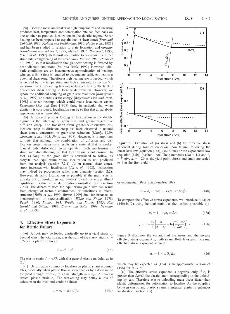
[38] Because rocks are weaker at high temperature and shearingproduces heat, temperature and deformation rate can feed back onone another to produce localization in the ductile regime. Shearheating has been proposed to explain ductile shear zones [Brun andCobbold, 1980; Fleitout and Froideveau, 1980; Hobbs et al., 1986]and has been studied in relation to plate formation and orogeny[Froideveau and Schubert, 1975; Melosh, 1976; Bercovici, 1993;Schott et al., 1999]. Heat must accumulate to overcome the directstrain rate strengthening of the creep laws [Poirier, 1980; Hobbs etal., 1986], so that localization though shear heating is favored bynear-adiabatic conditions [Bai and Dodd, 1992]. However, adia-batic conditions are an instantaneous approximation of heating,whereas a finite time is required to accumulate sufficient heat in apotential shear zone. Therefore a high heating rate is needed, whichis favored by low temperature and high strain rate. In section 7.1we show that a preexisting heterogeneity such as a brittle fault isneeded for shear heating to localize deformation. However, weignore the additional coupling of grain size evolution [Kameyamaet al., 1997] or stored elastic energy [Regenauer-Lieb and Yuen,1998] to shear heating, which could make localization easier.Regenauer-Lieb and Yuen [1998] show in particular that whenelasticity is considered, localization can be so fast that an adiabaticapproximation is reasonable.[39] A different process leading to localization in the ductile

regime is the interplay of grain size and grain-size-sensitivediffusion creep. The transition from grain-size-insensitive dis-location creep to diffusion creep has been observed in naturalshear zones, concurrent to grain-size reduction [Handy, 1989;Jaroslow et al., 1995; Jin et al., 1998]. However, it is importantto note that although the combination of diffusion and dis-location creep mechanisms results in a material that is weakerthan if only dislocation creep operated, each mechanism isstrain rate strengthening, so that localization is not ensured. Infact, as long as the grain size is constrained to follow itsrecrystallized equilibrium value, localization is not predictedfrom our analysis (section 7.2.1). As in natural shear zones,stress increases with localization [Jin et al., 1998], localizationmay indeed be progressive rather than dynamic (section 2.2).However, dynamic localization is possible if the grain size isinitially out of equilibrium and evolves toward the recrystallizedequilibrium value at a deformation-controlled rate (section7.2.2). The departure from the equilibrium grain size can resultfrom change of tectonic environment or transitions in micro-structure [Tullis et al., 1990; Rutter, 1999] due, for instance, tometamorphism or neocrystallization [White and Knipe, 1978;Beach, 1980; Rubie, 1983; Brodie and Rutter, 1985; FitzGerald and Stunitz, 1993; Brown and Solar, 1998; Newmanet al., 1999].

4. Effective Stress Exponentsfor Brittle Failure

[40] A rock may be loaded elastically up to a yield stress sybeyond which the total strain, e, is the sum of the elastic strain ee =s/G and a plastic strain ep:

e ¼ ee þ ep � ð13Þ

The elastic strain ee = s/G, with G a general elastic modulus as in(10).[41] Deformation commonly localizes as plastic strain accumu-

lates, especially when plastic flow is accompanies by a decrease ofthe yield strength from sy to a final strength sf = sy� �s over acritical plastic strain ec. The weakening may betray a loss ofcohesion in the rock and could be linear

s ¼ sy ��s ep=ec ð14aÞ

or exponential [Buck and Poliakov, 1998]

s ¼ sy ��s 1� exp �ep=ecð Þ½ � � ð14bÞ

To compute the effective stress exponents, we introduce (14a) or(14b) in (2), using the total strain e as the localizing variable c0:

ne ¼ 1� ecsy�e�s ; ð15aÞ

ne ¼ 1� ece

ss� sf

� lns� sf�s

� �� ð15bÞ

Figure 3 illustrates the variation of the stress and the inverseeffective stress exponent ne with strain. Both laws give the sameeffective stress exponent at yield:

ne ¼ 1� ecG=�s ; ð16Þ

which may be expected as (15a) is an approximate version of(15b) for s sy.[42] The effective stress exponent is negative only if ec is

greater than �s/G, the elastic strain corresponding to the unload-ing by �s. Therefore elastic unloading must occur faster thanplastic deformation for deformation to localize. As the couplingbetween elastic and plastic strains is internal, elasticity enhanceslocalization (section 2.5).

0 2 4 6 8 10 12 140

0.2

0.4

0.6

0.8

1

1.2

Total strain εG/σy

Str

ess

σ/σ y

0 2 4 6 8 10 12 14

-0.5

0

0.5

1

Total strain εG/σy

Inve

rse

effe

ctiv

e st

ress

exp

onen

t 1/n

e

εp=ε

cG/σ

y

yiel

d

σf /σy

a)

b)

Figure 3. Evolution of (a) stress and (b) the effective stressexponent during loss of cohesion upon failure, following thelinear loss law (equation (14a)) (solid line) or the exponential law(equation (14b)) (dashed line). The parameters (�s = 1/3 and ec= 7) give ne = �20 at the yield point. Stress and strain are scaledto 1 at the first yield.


[43] For �s = 20 MPa and G = 30 GPa, the minimum ec is oforder 0.6 � 10�3. Buck and Poliakov [1998] used ec = 0.03 to 0.3,or ne �450 to �45, to study localization of deformation at mid-ocean ridge spreading centers and produced realistic lookingabyssal hills.

5. Effective Stress Exponent for ElastoplasticMaterials

5.1. Flow Theory of Plasticity

[44] Before addressing localization for elastoplastic materials,we find it useful to review the basics of the flow theory of plasticityin two dimensions [Hill, 1950; Lubliner, 1990]. First, we define thestress and strain vectors

s ¼

sxxsxysyysyx

0BB@

1CCA; e ¼

exxexyeyyeyx

0BB@

1CCA: ð17Þ

The strain in (17) is the total strain, the sum of an elastic strain,which is related to the instantaneous stress by the stiffness matrix,D, and a plastic strain. The plastic strain accumulates when a yieldcriterion is verified. Here we assume that yielding follows a Mohr-Coulomb failure law:

f ¼ sII � sI sin j� c cos j ¼ 0 ; ð18Þ

where sI and sII are the first and second invariants of the stresstensor, j is the internal friction angle, and c is the cohesion(Figure 4) [Vermeer and de Borst, 1984]. The more familiarcriterion f = ss � sn tan j � c, with ss and sn the shear andtangential stresses on a failure plane, is equivalent to (18), assumingthat there exists a fabric of planes in the material with their normaloriented at qq = p/4 � j/2 from the direction of the leastcompressive stress, the most favorable orientation for failure. If thefabric is pervasive, the material is considered a continuum. We donot include explicit hardening or weakening in the failure criterion.

[45] The direction of plastic strain increments is determined bythe flow potential g; plastic strain increments are proportional to

rsg; where r

sdenotes the gradient taken in an orthonormal base

describing the space of stress vectors. It is customary to take

g ¼ sII � sI sin y ; ð19Þ

where y is the dilation angle [Vermeer and de Borst, 1984; Mandl,1988]. The strain field resolved on a plane includes generally shearand dilatant motion. Hence the plastic strain increment is coaxial tothe stress increment only if the plane is at an angle qy = p/4 � y/2from the least compressive stress (Figure 4a). If plasticity isnonassociated (j 6¼ y), that plane is different from the failureplane. Therefore the strain and stress increments are incompatible,which leads to localization [Rudnicki and Rice, 1975; Vermeer andde Borst, 1984].[46] The amplitude of the elastoplastic strain increment is such

that the material stays at yield. Hence, increments of stress andtotal strain are related by ds = M� de (Appendix A1) [Vermeer andde Borst, 1984], with

M ¼ D � 1�rsg

rsf T � D

rsf T � D � r

sg

24

35 ; ð20Þ

5.2. Localization in a Continuous Elastoplastic Medium

[47] We first address localization in a continuous mediumloaded elastically to yield. Potential discontinuities will be consid-ered in section 5.3. Loading is achieved by cumulative strainincrements de = E de, where E is a shape vector and de is themagnitude of each increment. The second strain invariant is used asde, and E is parameterized by v, the ratio of volume change to de,and by the angle q between the reference axes and the principaldirections of strain:

E ¼ 1

2

vþ cos 2qsin 2q

v� cos 2qsin 2q

0BB@

1CCA � ð21Þ

Mos

t com

pres

sive

stre

ss

Least compressivestress

ψ

θ

a)

σ0

ρ=1

ρ=0.5ρ=0

ρ=-1

σII

σI

ϕ

c cos ϕ

b)

θ+ψ/2−π/4

Figure 4. (a) Geometry used in the treatment of elastoplastic materials. The parameter q is the angle between theprincipal stress directions (large arrows) and the normal to a reference plane (thick line). Shearing on that plane isaccompanied by dilation, so that the direction of motion on that plane makes an angle y, the dilation angle, with theplane. The principal strain directions (smaller arrows) differ from the principal stress direction unless qj = qy. (b)Loading trajectories. The prestress is s0, and r is the ratio between the first and second invariants of stress incrementsup to the yield envelope (thick line). When the loading is defined as a strain (section 5.2), it is parameterized by s0and v, the ratio of first to second strain, which is related to r before yielding by r = (1 + l/G) v, with l and G as theLame parameters.


Loading in pure shear corresponds to v = 0 and uniaxial loadingcorresponds to v = 1 (one principal strain increment is null). Usingthe elastic stiffness matrix D and a possible prestress s0, the stressat yield is s0+ nD � E de, with n the number of increments neededto reach the yield point. Any value of v is admissible if thecohesion is nonzero (Figure 4b). The Lame parameters l and Gand their ratio r = l/G characterize D (Appendix A1). Nolocalization is possible during the elastic loading stage (ne = 1).[48] At yield, a new strain increment brings a stress increment

ds = M � E de, with M defined in (20). As s is a tensor, we mustdefine a measure s against which we test for localization. Hence theeffective stress exponent ns measures the possible weakening of s �s that arises from a change of de. Using (2) and (20), we obtain

1

ns¼ s �M � E

s�s0n de

þ s � D � E � ð22Þ

[49] For the sake of simplicity, we assume in what follows thats0 is 0, or at least transparent to the measure s, as is the case forhydrostatic pressure if s measures a shear stress. We investigatedseveral measures of stress and present our results for the localizationof shear stress sxy (sT = [0,1,0,0]) and normal stress sxx (sT =[1,0,0,0]). The effective stress exponents for these measures are

nxy ¼1þ 1þ rð Þ sin y sin j

1þ rð Þ sin y� vð Þ ð23aÞ

nxx ¼ nxycos 2q� v 1þ rð Þcos 2qþ 1=sinj

; ð23bÞ

respectively. Each effective stress exponent addresses the localiza-tion of the external strain imposed on an elastoplastic material, inrelation to a given internal measure of stress. Hence it does notconcern the behavior of a potential shear zone inside the materialbut rather how the material that includes that shear zone is seenfrom a larger scale.[50] Localization of strain and sxy occurs when sin y < v,

regardless of whether the material is associated or not; localizationdemands that the volume changes associated with shearing on theplane are different for the loading system (expressed by v) and theelastoplastic material (expressed by sin y). In agreement with ourresult, Vermeer and de Borst [1984] determined that y must benegative (compaction) for localization to occur in a pure shear strainfield (v = 0). For a Poisson solid (r = 1) with j = 30� and y = 0�, as istypical or rocks, and v between 0 and 1, 1/nxy is between 0 and�1/2.[51] Although localization using sxy does not depend on the

orientation of shearing planes, localization using sxx does. Hencethe apparent weakening of the material of the material is aniso-tropic. Figure 5 shows how nxx varies with q for different values ofv. Axial splitting (q = 0) and compaction bands (q = p/2) arefavored over shear failure, as nxx passes through extrema at q = jp/2with j an integer. Compaction bands are further unlikely as theyrequire v < �1/(1 + r). On the other hand, axial splitting is a realpossibility as it needs 1/(1 + r) > v > sin y. However, the effect ofthe prestress remains to be determined: In experiments, axialsplitting is prevented by a small confining pressure.[52] It may be argued that localization requires nxx = nxy < 0 as,

in that case, the strength lost during localization is tensor coaxialwith the stress increments during the loading. However, nxx = nxy <0 is verified only if sin y sin j (1 + r) < �1, which requires thatplastic flow be compactive (y < 0).

5.3. Localization in an Elastoplastic MediumWith a Planar Discontinuity

[53] We now consider the case of an elastoplastic material witha potential planar discontinuity, as in the bifurcation analysis or

Rudnicki and Rice [1975]. The material is loaded elastically anduniformly to yield, at which point the discontinuity may separate aportion of the material that behaves elastoplastically from anotherthat remains elastic [Vermeer, 1990]. Elastoplastic strain incre-ments are given by (20). No explicit weakening or hardening isincluded in the flow law, but the activation of the discontinuitymay reduce the overall strength of the material in which it isembedded; as in section 5.2, we address only the apparent behaviorof the material as seen from a larger scale.[54] The loading is now defined by stress increments ds =

SdsII, with dsII the increment of the second invariant of the stresstensor and S a shape vector parameterized by r, the ratio betweenthe variation of first and second stress invariants, and q the anglebetween the normal of the plane and the direction of leastcompressive stress (Figure 4b):

S ¼ 1

2

r� cos 2qsin 2q

rþ cos 2qsin 2q

0BB@

1CCA ; ð24Þ

[55] We define a reduced plastic increment matrix M0 thatrelates the free components of strain increments within the band,dexx and dexy, to dsII. The other component of the strain incrementtensor, deyy, and the components dsxx and dsxy of the stressincrement tensor are transmitted across the potential discontinuity(Appendix A2) [Rudnicki and Rice, 1975; Vermeer, 1990]. We thentest for the localization of dexy and dexx for which we define theeffective stress exponents nxy and nxx, respectively.[56] Assuming no prestress (e = D�1� SdsII) and using de =M0 �

SdsII in (2), we obtain (Appendix A2 and Figure 6)

nxy ¼ cos22q� sin jþ sin yð Þcos 2qþ sin jh

sin y

þ 2þ r

1þ r1þ r sin jð Þ

icos 2q� sin jð Þ

hcos 2q� sin yð Þ

i�1

ð25aÞ

0 20 40 60 80Projection angle θ

nxx

-20

-15

-10

-5

0

5

10

15

20

Effe

ctiv

e st

ress

exp

onen

t ne

nxy

ν=1.0

ν=0.3

ν=0.0

ν=-1.0

Figure 5. Effective stress exponent of an elastoplastic materialwithout discontinuity for localization of strain and either (left)shear stress or (right) normal stress. Stress is resolved on a planewith its normal at an angle q to the least compressive stress; v is theratio of volumetric strain over the second invariant of strain. Solidline is v = 1; dashed line is v = 0.2; dotted line is v = 0; and dash-dotted line is v = �1. Prepared for j = 30�, y = 6�, r = 1, and noprestress.


nxx ¼ 1þ rð Þcos3 2q�

þ r� 1þ rð Þ sinjþ sinyð Þ½ �cos2 2qþ 2þ 1þ rð Þsinj sinyþ r sinj� sinyð Þ½ �cos 2qþ2 1þ rð Þsinyþ r 3þ 2rð Þsinj sinyg�f cos 2q� sinjð Þ cos 2q� sinyð Þ½r� 1þ rð Þcos 2q�g�1:

ð25bÞ

[57] Both 1/nxy and 1/nxx are null when the determinant of M0

is zero, that is, when the discontinuity is oriented at qj = p/4 �j/2 and qy = p/4 � y/2 from the loading directions. Thiscondition marks the bifurcation criterion of Rudnicki and Rice[1975]. Although the material does not weaken at this point, itallows the formation of a discontinuity [Vermeer, 1990]. Inaddition, 1/nxx is null as the elastic strain increment change signsat cos 2q = r/(1 + r). The numerator of nxx can also be zero forrealistic conditions (Figure 6b), but the numerator of nxy does notchange sign unless j approaches 90� and y approaches �90�,which are not unrealistic values (Appendix A2).[58] Localization of exy is most efficient at qa = p/4 � (j + y)/4

where 1/nxy is minimum [Vermeer, 1990]. The localization of exx isstrongest localization where 1/nxx ! �1. However, this drasticlocalization may not occur spontaneously because nxy is positivefor these values (not all components of the deformation field tendto localize) and, as it is not related to the condition for spontaneousdiscontinuity formation, |M0| = 0 [Rudnicki and Rice, 1975], therequired discontinuity may be unavailable in the material. If thereis a preexisting discontinuity at the angle for which 1/nxx ! 1, thedrastic localization of the normal strains may happen. This mightexplain the compaction bands documented by Antonellini et al.[1994] and Olsson [1999], as 1/nxx ! 1 at q = 90� for r = 1 and r= 0. However, this explanation is unlikely because compactionbands are observed in materials where r 6¼ 0 and because thedivergence of nxx is suppressed with confining pressure, whereascompaction bands are observed only with significant confiningpressure [Olsson, 1999]. Compaction bands are more likely tooriginate at the vertex between two yield envelopes [Issen andRudnicki, 2001; Wong et al., 2001], a feature of the yield criterionthat we do not consider herein.[59] In Figure 7 we present a section through the maps of

effective stress exponent of Figure 6 at q = qa, where both nxy andnxx are negative and 1/nxy is minimum. For realistic rock param-eters (r = 1, q = 30�, y = 6�), 1/nxy increases with r from roughly�0.0525 to �0.0175, while 1/nxx decreases to �0.02. A good

value where both effective exponents are similar is ne �50, andr 0.75.

6. Effective Stress Exponents for Localizationin Frictional Materials

6.1. Static and Dynamic Friction

[60] A frictional material is one that deforms by sliding onmany faults, so that it may be viewed as a continuum with astrength obeying the friction laws. Its deformation field localizes asa particular fault becomes more active than the others. Thisrequires that active faults be weaker than less active or inactiveones, possibly because the dynamic coefficient of friction, md, islower than the static coefficient of friction, ms. Rabinowicz [1951]proposed that the transition from ms to md occurs over a criticalsliding distance DC. If the coefficient of friction decreases linearlywith sliding distance ds, we obtain

ne ¼ 1� msms � md

DC

d; d < DC ; ð26Þ

with d the imposed displacement, different from ds because ofelastic deformation. This formula is similar to (14a) for localizationupon failure (Figure 3) with the loss of strength interpreted as adecrease of coefficient of friction rather than as a loss of cohesion.In either case, external coupling with a stiff loading system canprevent localization (section 2.5), as is done experimentally tostudy the details of the weakening occurring upon failure or faultactivation [Cook, 1981]. From (12), stabilization occurs when k,the rigidity of the loading apparatus, exceeds (ms�md)/DC, which isthe rate at which m decreases with displacement [Scholz, 1990,equation 2–24].[61] In order to model the healing faults as their activity ceases

it may be better to associate the weakening of active faults withtheir sliding velocity V. Dieterich [1972, 1978] proposed that thecoefficient of friction m during sliding depends on the shearingvelocity V as

m ¼ m0 � c � ln V=V0ð Þ ð27Þ

with m0 and V0 the reference coefficient of friction and velocity andca material constant. Using (2) with V as c0 and m as s, theeffective stress exponent is

0 10 20 30 40 50 60 70 80 90-1

-0.8-0.6-0.4-0.2

00.20.40.60.81

Discontinuity angle θ

Inverse effective stress exponent 1/nxx

Load

ing

para

met

er ρ

b)

0.4

0.1

0.3

0.20.1

0 10 20 30 40 50 60 70 80 90-1

-0.8-0.6-0.4-0.2

00.20.40.60.81

Discontinuity angle θ

Inverse effective stress exponent 1/nxy

Load

ing

para

met

er ρ

a)

0.3

0.2

0.1 0.1

0.6

0.5

0.4

0.3

0.2

Figure 6. Contours of inverse effective stress exponent for localization of (a) shear strain and (b) normal strain foran elastoplastic material with a discontinuity at angle q from the principal directions of loading. The loading parameterr is ratio of first to second invariant of the stress perturbation. The thick lines mark changes of sign of ne, withcontours at every 0.01 to a maximum of 2. The region of negative stress exponent is shaded. the darker shading showswhere both nxy and nxx are negative. It is assumed that r = 1, j = 30�, and y = 6� and no prestress.


ne ¼ �m=c: ð28Þ

For values typical of rocks (m 0.75 and c 0.003), ne is �250.[62] Localized velocity can be expressed by localized regions

that deform more or less uniformly in time (faults, intense shearzones) or nonlocalized regions where deformation is temporallylocalized (stick-slip motion, earthquakes). In reality, both occur,and the interpretation of localized velocity may differ depending onwhether one is interested in earthquake mechanics or tectonicmodeling.

6.2. Rate- and State-Dependent Friction

[63] Transient effects of frictional behavior can be incorporatedthrough the formalism of rate- and state-dependent friction laws(RSDF) [Scholz, 1990; Marone, 1998], where the coefficient offriction m depends on the displacement velocity V and on a statevariable q, which may indicate the age of granular contacts [Diet-erich, 1979] or the integrated slip history of the fault [Ruina,1983]. The friction law

m ¼ m0 þ a ln V=V0ð Þ|fflfflfflfflfflfflffl{zfflfflfflfflfflfflffl}Direct Effect

þ b ln V0q=Dð Þ|fflfflfflfflfflfflfflffl{zfflfflfflfflfflfflfflffl}State Evolution

ð29Þ

is coupled to an evolution law for the state variable, of the formproposed by Dieterich [1979]:

dqdt

¼ 1� V qD

ð30aÞ

or, alternatively, by Ruina [1983]:

dqdt

¼ �V qD

lnV qD

� �; ð30bÞ

where D is a critical distance related to the macroscopicstructure of the fault gouge and possibly to DC encountered insection 6.1. The parameters V0 and m0 are reference values ofsliding velocity and friction coefficient, and a and bare materialparameters. In steady state, q = D/V in either case, and (29)becomes (27), with c = b–a.

[64] The rheological system involved in the RSDF laws iscomposed of the two variables, q and V. The velocity is thequantity that localizes in out treatment of frictional materialsobeying the RSDF laws. As the state variable depends onthe integrated history of velocity, we must specify a studycase, whereby a perturbation in velocity is sustained for alltime t > 0. Initially, the state variable is at equilibrium. Weobtain (Appendix B)

1

ne¼ 1

ma� b

D

qV1� exp �Vt

D

� �� : ð31Þ

[65] An illustrative example evolution of ne upon perturbationof sliding velocity is given in Figure 8. Initially, the effective stressexponent is positive because of the stabilizing direct effect (a > 0).However, if b > a, ne changes sign after timr tc because of theevolution of the state variable, with

tc �D

Vln 1� a

b

� �� ð32Þ

For velocity to localize in a material obeying the RSDF laws thevelocity perturbation must be held for at least tc.[66] In the infinite time limit the effective stress exponent tends

toward the value for steady state sliding (equation (28), ne �250). This value is probably the most relevant for large-scalegeodynamics, where long timescales are involved. However, earth-quakes mechanics are dominated by the transient behavior [Diet-erich, 1992; Marone, 1998]. If the RSDF includes more than onestate variable [Gu et al., 1984; Gu and Wong, 1994; Blanpied et al.,1998], it may be stable in the steady limit, but there can be a timewindow when the material is apparently weakening [Montesi et al.,1999].

6.3. Fault Gouge and Pore Fluid Effects

6.3.1. Apparent coefficient of friction and dilatancy.[67] One physical aspect of fault gouge mechanics that mayexplain the weakening of active faults is the dilation of gougeupon shearing [Frank, 1965; Orowan, 1966; Marone et al., 1990].Gouge dilation works against the effective normal stress, se = sn �pf, where sn is the normal stress imposed on the fault and pf is thepressure of a pore fluid within the gouge. The energy needed fordilation is provided by the loading, in particular by the shear stresst. Therefore, the apparent friction coefficient ma = t/se is higher

-1 -0.8 -0.6 -0.4 -0.2 0 0.2 0.4 0.6 0.8 1-0.05

-0.04

-0.03

-0.02

-0.01

0

Loading parameter ρ Inve

rse

effe

ctiv

e st

ress

exp

onen

t 1/n

e

1/nxx

1/nxy

Figure 7. Effective stress exponents as a function of loadingparameter r for the same case as Figure 6 and perturbation angle q =p/4 �(j + y)/4 for which localization is strongest in the regionwhere both nxy and nxx are negative. Prepared for j = 30� an y = 6�.

0 0.5 1 1.5 2 2.5 3 3.5 4 4.5 5-0.5

0

0.5

1

Time tV/DInve

rse

effe

ctiv

est

ress

expo

nent

1/n e

b=a/2b=3a/2

Figure 8. Evolution of the inverse effective stress exponent aftera jump of sliding velocity using the rate- and state-dependentfriction laws. Solid line is b = 3a/2, steady state weakening.Dashed line is b = a/2, steady state velocity strengthening. Thethick horizontal segments indicate the steady state limit (equations(27) and (28)). The vertical line is the approximate tc limit from(32). It is assumed that a = 1, m0 = 1, and dv/v = 0.01.


than the actual friction coefficient m. On the basis of suchthermodynamic considerations, Frank [1965] proposed

ma ¼ mþ dv=dg ; ð33aÞ

with v the volume of the gouge and g the shear strain [see alsoEdmond and Paterson, 1972; Marone et al., 1990]. In contrast,Orowan [1966], taking into account the change of direction of themicroscopic friction force between gains as they climb onto oneanother, derived

ma ¼mþ dv=dg

1� m dv=dg� ð33bÞ

Localization is possible if the dilation rate dv/dg decreases withstrain [Frank, 1965; Edmond and Paterson, 1972; Fischer andPaterson, 1989; Marone et al., 1990].[68] On the other hand, dilation decreases the pore fluid

pressure and therefore increases the effective normal stress [Rey-nolds, 1885; Frank, 1965], thereby stabilizing slip [Rice, 1975;Rudnicki, 1979]. The capacity of the fluid is defined as Kf = �dpf /dv. Physically, the fluid capacity represents not only the compres-sibility of the fluid, which is very small if the pore fluid is liquid,but also the ability of the fluid to circulate in the gouge and toexchange with the surrounding wall rocks [Rudnicki, 1979; Rud-nicki and Chen, 1988]. If the gouge is highly permeable, fluidpressure gradients cannot be sustained and Kf tends toward zero,even if the fluid is incompressible.[69] This rheological system is composed of the gouge

volume, the shear strain, and the pore fluid pressure. We testfor the localization of the shear strain, g, with respect to theshear stress. In addition, we consider only the initiation ofsliding, so that g = t/G, with G the shear modulus of intactgouge. Hence the effective stress exponents is

1

ne¼ 1

G

dhadg

se � hadpf

dg

� �� ð34Þ

Replacing ma by (33a) and (33b), respectively, and using Kf =�dpf /dv, we obtain

1

ne¼ se

G

d2v

dg2þ Kf

G

dv

dgmþ dv

dg

� �ð35aÞ

for Frank’s [1965] theory, and

1

ne¼ se

G

1þ m2

1� m dv=dgð Þ2d2v

dg2þ Kf

G

dv

dg

mþ dv=dg

1� m dv=dgð35bÞ

for Orowan’s [1966] theory. Figure 9 shows how the effectivestress exponent varies in function of the dilation rate for severalvalues of the parameter d2v/dg2 se/Kf. The dilation rate is limited todv/dg > �m for Frank’s theory and 1/m > dv/dg > �m for Orowan’stheory by the condition that ma > 0.[70] If the gouge is fully drained (Kf = 0), localization requires

that d2v/dg2< 0, i.e., that the dilation rate decrease with strain[Frank, 1965; Marone et al., 1990]. However, for Frank’s theory,the stabilizing effect of pressure changes brings an upper limit tothe dilation rate that can localize. Beyond that, the pressure changedominates and localization is impossible. However, changes ofpore fluid pressure can help the system localize if the gougecompacts. Indeed, the pore fluid pressure increases as the gougecompacts, supporting more of the normal stress. Hence localizationis possible in a compacting gouge (dv/dg < 0) if d2v/dg2 sn/Kf < m2/4 (Figure 9). Indeed, dynamic weakening of an undrained fault

gouge undergoing compaction was observed by Blanpied et al.[1992]. Changes of pore fluid pressure has less effect in Orowan’stheory. In particular, they cannot change the domain of dilation ratethat localize or not, although localization is generally less strongwhen the pore fluid effects are taken into account.[71] More rigorous treatments of fluid flow in a deforming

matrix exist [Rudnicki and Chen, 1988; Segall and Rice, 1995]. Forinstance, Sleep and Blanpied [1994] showed that compaction,resulting from ductile creep in the fault gouge driven by theoverpressurization of the pore fluid, is sufficient to destabilizefault slip. At high temperatures, the matrix is assumed to deformviscously [McKenzie, 1984; Spiegelman, 1993; Bercovici et al.,2001a]. In that case, porosity (or damage) and surface tensioninteract to concentrate a fluid phase to a localized band [Bercoviciet al., 2001b]. How the band would affect the strength of thematerial in which it forms has not yet been discussed.

6.3.2. Pore fluid heating. [72] Pore fluids promotelocalization if their pressure increases with either strain orstrain rate. In the previous paragraph, pressure increased if thegouge compacted. Alternatively, pore fluid pressure increases asthe fluid dilate if it is heated by the deformation. Shaw [1995],following Sibson [1973] and Lachenbruch [1980], proposed thatthe normal stress sn on a fault gouge decreases linearly with theheat Q as

sn ¼ s0n � aQ ; ð36Þ

with a a coefficient and sn0 the value without deformation. Heat

may diffuse away over the timescale td but is replenished at a rateproportional to mv, where v is the shearing velocity on the fault.The approximations that td is small (steady state conductive) orthat td is large (adiabatic heating) result in weakening withvelocity v or slip s, respectively [Shaw, 1995]. The correspondingexpression for s are

s ¼ ms0n1þ tdmav

; ð37aÞ

s ¼ ms0nexp �am sð Þ ; ð37bÞ

-0.5 0 0.5 1 1.5 2-20

-15

-10

-5

0

5

10

15

20

d2v/dγ2.σe /Kf

-30

-6

3

Dilation rate dv/dγ

Inve

rse

effe

ctiv

e st

ress

exp

onen

t (G

/Kf 1

/ne)

µ=0.8

dv\d

γ=µ

com

pact

ing

dila

ting

Figure 9. Inverse effective stress exponent for a fault gouge as afunction of the compaction/dilation according to Frank [1965](thick lines) or Orowan [1966] (thin lines) theories with m = 0.8and several values of the dilation rate d2v/dg2, pore fluid pressurepf, and fluid capacity Kf.


with effective stress exponents

1

ne¼ �1

1þ 1=tdma v; ð38aÞ

1=ne ¼ �am s � ð38bÞ

The effective stress exponent is negative for all finite a. As a is notdetermined, it is difficult to address whether elastic effects wouldstabilize this mechanism of localization or not.

7. Effective Stress Exponent for LocalizationDuring Ductile Creep

7.1. Shear Heating

7.1.1. General analysis. [73] Shearing a rock at the rate _eand stress s (rock strength) releases energy by viscous dissipation,a fraction b of which is converted into heat H:

H ¼ bs_e � ð39Þ

As the strength of ductile rocks is temperature-activated, the heatanomaly due to a local increase of strain rate can weaken the rockand localize the strain rate. The rheology of ductile rocks is suchthat

s ¼ B_e1=n exp 1=nqð Þ ; ð40Þ

where n is the stress exponent (not to be confused with the effectivestress exponent ne) and B is a material constant. The rheologicaltemperature q is defined as q = TRG/Q, with T the absolutetemperature, RG the gas constant, and Q the activation energy. Weignore for now additional dependencies of B on grain size (fordiffusion creep), chemical activity, etc. Then, (40) introduced in (2)with _e as c0 gives

1

ne¼

_es

@s@ _e

þ @s@q

@q@ _e

� �¼ 1

n1�

_eq2

@q@ _e

� �� ð41Þ

[74] The temperature is influenced by the strain rate through theheat produced by shearing. Perturbing the heat production by dHchanges the temperature by

dT ¼ T dH ; ð42Þ

where the coefficient T is the heat retention factor that may dependon the size of the perturbation and the time t since its onset, as wellas on the thermal properties of the rock and the geometry of theperturbation. For instance, if heat retention is adiabatic, we have

T ¼ t=rC ; ð43Þ

with r the density and C the thermal capacity of the rock. If heatconduction is included, the temperature anomaly depends ondistance from the perturbation [Carlslaw and Jaeger, 1959]. Onlythe temperature change at the location of the perturbation, dT, isimportant for shear-heating feedback. We define dT as the averagetemperature anomaly within a thickness d, small but finite, of theperturbation origin, which is identified with the perturbation‘‘size’’. More specifically, we use the formula for a planar heatsource continuously active from time 0 (onset of the perturbation)to t [Carlslaw and Jaeger, 1959, equation 10.4.9] to compute

T ¼ t

rCerf

d

2ffiffiffiffikt

p þ d

2ffiffiffiffikt

p exp�d2

4kt� d2

2kterfc

d

2ffiffiffiffikt

p�

; ð44Þ

with k the thermal conductivity of the material.[75] The linear relation between the anomalies of heat produc-

tion and temperature (42) is valid when dH is small. It gives

@T

@ _e¼ T @H

@ _e¼ bT s 1þ 1

n

� �: ð45Þ

Then the effective stress exponent (41) becomes

1

ne¼ 1

n1� 1þ 1

n

� �Hq2

� ; ð46Þ

where H is a nondimensional heat production defined as

H ¼ T HRG=Q � ð47Þ

[76] In the q–H space, contours of effective stress exponentfollow parabolas (Figure 10). High temperatures are stable becausethe low strength of the rock generates only a little heat; shearheating is not efficient enough to overcome the direct strengtheningeffect of increasing the strain rates. As H depends on stress andthus on temperature by (40) H and q are not independentlycontrolled.

7.1.2. Application to Earth materials. [77] The importanceof localization by shear heating in the lithosphere is evaluatedusing a set of experimentally derived rock rheologies. We use theflow laws of Gleason and Tullis [1995] for quartzite, Caristan[1982] for diabase, Mackwell et al. [1998] for ultradry diabase, andKarato et al. [1986] for olivine in the dislocation creep regime. Inaddition, we use the results of Dimanov et al. [1998] forplagioclase deforming in the diffusion creep regime, assuming afixed grain size of 0.1 mm.[78] The effective stress exponent for shear heating is shown in

Figure 11 as a function of temperature, assuming a strain rate of10�15 s�1 and t 104 K W�1. If the heat retention is total(adiabatic conditions), t = t/rC 104 K W�1 corresponds roughlyto a perturbation active during 1000 years, in a rock of density r 3000 kg m�3 and heat capacity C 1000 J kg�1 K�1.

0 0.1 0.2 0.3 0.4 0.5 0.6 0.7 0.8 0.9 10

0.2

0.4

0.6

0.8

1

1.2

1.4

1.6

1.8

2

Temperature θ=TR/Q

Hea

t Gen

erat

ion

=

βσε

R/Q

0

0.3-0

.5

-1

-2

Figure 10. Contours of inverse effective stress exponent 1/nefor shear heating with n = 3, as a function of thegeneralized coordinates q and H (see section 7.1.1). Contoursare plotted every 0.1 down to �2. Contours are dashed wherene > 0 (no localization). The thick line marks the transition tolocalization (1/ne = 0).


Although very strong localization is predicted (1/ne < �1), itrequires temperatures below 300�C except for the example ofdiffusion creep. However, ductile flow is replaced by brittle failureor a high stress deformation mechanism such as Peierl’s creep atthese temperatures. If T was higher, the maximum temperature forlocalization would increase, but heat losses by conduction could beimportant, as the implied time to hold the perturbation would belonger. Higher strain rates also help localization, but they do notoccur spontaneously in the Earth’s lithosphere.[79] A more interesting question is what heat retention factor t

is needed for localization, given a flow law, the deformation rateand the ambient temperature. Once t is known, we invert (43) or(44) to obtain the minimum time (or, equivalently, the criticalstrain ec) during which the perturbation has to be active to allowlocalization (Figure 12). Because localization is favored at lowtemperature, we use the temperature at the brittle-ductile transi-tion for a given flow law, calculated following Brace andKohlstedt [1980] for a geotherm of 30 K km�1 and assuminghorizontal shortening. Therefore, the temperature increases withstrain rate and varies with rock type.[80] Under the adiabatic assumption, localization may occur

after 3–6% strain, with little dependence on the strain rate(Figure 12). Heat loss can only increase the time during whicha perturbation must be held before it triggers localization. Toinclude heat losses in the analysis, we assume a planar perturba-tion (equation (44)), k = 1 mm2.s�1, and follow one of twoassumptions regarding the perturbation size d:

1. The perturbation width does not depend on strain rate: d = 1km. The adiabatic assumption is valid for large strain rates(Figure 12), but for _e < 10�14s�1, the time for which theperturbation must be sustained before localization occurs isprohibitively long.

2. The perturbation width is inversely proportional to thestrain rate so that the velocity across the perturbed region is afraction f = 1% of a total velocity v = 30 mm yr�1 typical ofplate tectonics:

d ¼ fv=_e � ð48Þ

The adiabatic limit occurs at small strain rate, where the perturba-tion width is large. The time for localization is always longer than 1Myr.

[81] Localization is improbable at low strain rates. The adiabaticlimit requires perturbation widths in excess of 100 km at 10�16 s�1.Even if the plane approximation made to derive (44) remainedvalid for shear zones so wide, holding such a perturbation for atleast 1 Myr, the minimum time required for localization, wouldprobably indicate a preexisting material heterogeneity. Hence thelocalization should be regarded as inherited rather than dynamic.On the other hand, high strain rates permit localization of thinperturbations after a time short compared to tectonic timescales. Akilometer-thick shear zone can be considered adiabatic at strainrates in excess of 10�12 s�1. Such strain rates occur in thecontinuity of brittle faults. Then localization requires perturbationsheld for only 1000 years, which is of the same order as theearthquake cycle.[82] We conclude that shear heating does not arise spontane-

ously in the lithospere but requires preexisting heterogeneities. Inparticular, it is possible beneath seismogenic faults. The relation ofductile shear zones and brittle faults has been pointed previouslyfrom field evidence [Ramsay, 1980; Sibson, 1980; Wittlinger et al.,1998]. Certainly, some additional feedback processes may increasethe likelihood of localization. In particular, Regenauer-Lieb andYuen [1998] included elasticity and showed that a thermal crackcan develop after <1 Myr, fed by the release of stored elastic strainenergy. However, other feedback processes that we also neglectedhere can stabilize localization.

7.2. Onset of Diffusion Creep

[83] Several deformation mechanisms can coexist in ductilerocks. For instance, dislocation creep and diffusion creep involvethe motion of two different types of microscopic defects [Ranalli,1995]. They probably add to one another, although one oftendominates the total strain rate. As diffusion creep depends on grainsize, and the grain size may evolve due to dislocation motions, it ispossible to devise a feedback mechanism by which ductile rockssoften. But do they weaken as well? Is the effective stress exponentnegative? In what follows, we first assume that the grain sizeadjusts instantaneously to its stress-dependent recrystallized equi-

0 100 200 300 400 500 600 700 800 900 1000-1

-0.8

-0.6

-0.4

-0.2

0

0.2

0.4

0.6

0.8

1

Temperature (˚C)

Inve

rse

effe

ctiv

e st

ress

exp

onen

t 1/n

e

GT

DiCa

MCKw

Figure 11. Application of shear heating feedback to several rocktypes, assuming _e= 10�15 s�1 and T = 104 K W�1. Flow lawsare GT, quartzite without melt [Gleason and Tullis, 1995]; Ca,diabase [Caristan, 1982]; Di, plagioclase in diffusion creep regime,with 0.1 mm grain size [Dimanov et al., 1998]; MC, dry Columbiadiabase [Mackwell et al., 1998]; Kw, synthetic olivine aggregates[Karato et al., 1986].

10-18 10-16 10-14 10-12 10-10 10-80.01

0.1

1

10

Strain Rate (s-1)

Crit

ical

str

ain

1 ye

ar

1 ka

1 G

a

1 M

a

GT

DiCa

MCKw

Adiabatic

Constantperturbation

sized 2/κ=1012s

Constantboundaryvelocity(fv)2/κ=10-16s-1

Figure 12. Critical strain for localization by shear heating as afunction of strain rate with various flow laws (style matchingFigure 11) at the brittle-ductile transition assuming a 30 K km�1

geotherm and horizontal compression. The lowest set correspondsto adiabatic heating. The others include conduction, assumingeither fixed perturbation size (critical strain increasing at low strainrate) or fixed boundary velocity (critical strain increasing at highstrain rate). The thin diagonal lines show the time needed to reachthe instability at the unperturbed strain rate.


librium value and find that dynamic localization is impossible.When the equilibrium assumption is relaxed, localization throughgrain-size feedback is allowed.

7.2.1. Grain size at equilibrium. [84] The total strain rateof a rock undergoing simultaneously dislocation and diffusioncreep, _e, is the sum of a dislocation creep strain rate

_eD ¼ ADsn ; ð49Þ

and a diffusion creep strain rate

_eG ¼ AGd�msp ; ð50Þ

where AD, AG, n, m, and p are material parameters and d is thegrain size of the material. Additional dependencies on temperature,chemical composition, water and oxygen fugacity, etc., areignored.[85] Stress-dependent dislocation motion induces recrystalliza-

tion of grains that competes with kinetic grain growth, so that thegrain size evolves toward an equlibrium value D:

D ¼ D0s�r � ð51Þ

If grain size evolution is rapid, d = D. The effective stress exponentis then derived from (2) with _e ¼ _eD þ _eG as the localizingvariable:

ne ¼s_e

@ _e@s

þ dD

ds@ _e@d

� �¼ nþ pþ mrð ÞR

1þ Rð52Þ

with R the ratio of strain rate accomodated by diffusion creep overthe strain rate accommodated by dislocation creep:

R ¼_eG_eD

¼ AGD�m0

AD

spþmr�n � ð53Þ

[86] The effective stress exponent is always positive, regard-less of the stress or the temperature; the latter enters in thecoefficients AD and AG. In fact, ne is bounded by n at low stress

(dislocation-dominated limit) and p + mr at high stress (diffusion-dominated limit) (Figure 13). Dislocation creep dominates at lowstress if p + mr > n because the large equlibrium grain sizemakes diffusion creep inefficient. The alternative assumption thatthe grain size is fixed at an initial value gives (52) as well, withr = 0. However, diffusion creep dominates at small strains if dis fixed [Karato et al., 1986; Handy, 1989; Jin et al., 1998].Weakening (ne < 0) never occurs because neither the dislocationcreep law nor the diffusion creep law weaken individually.[87] Although dynamic localization is not possible, the effective

stress exponent is always more than 1 and increases with stress.Hence progressive localization is possible. We recall from section2.2 that progressive localization requires that a perturbed materialis softer than in its initial configuration. Hence a further overallincrease of stress activates preferentially the perturbed location.However, the initial perturbation is not able to start a runawayprocess in that material. A localized shear zone may develop butonly if externally applied stress increases. Indeed, Jin et al. [1998]documented that the stress in a natural shear zone was higher thanin its surroundings; localization by grain-size feedback may beprogressive. In that case, localized shear zones are little more thanflow markers and do not influence significantly large-scale tec-tonics unless another localization process is simultaneously active.

7.2.2. Nonequilibrium grain size. [88] In section 7.2.1 thegrain size was fixed at its equilibrium value D (equation (51)).However, this assumption may not be valid if the stress or thetemperature vary rapidly due to tectonic motions [Kameyama etal., 1997; Braun et al., 1999] or if grain nucleation is important.We now suppose instead that the grain size of the material isinitially at d0 6¼ D and evolves toward equilibrium. A perturbationin strain rate changes both the equilibrium grain size and the rate ofgrain-size evolution, so that a perturbed location may appearweaker after a given time.[89] Following Kameyama et al. [1997] and Braun et al.

[1999], we assume that the grain size evolves toward the equili-brium value D according to

_d

dt¼ �

_eDeT

d � Dð Þ ; ð54Þ

where eT is a critical strain. Unlike previous authors, we includeonly the strain rate accommodated by dislocation creep in (54):Grain size evolves only due to dislocation motion. Then the grainsize d at time t is

d ¼ d0 �Z t

0

_eDeT

d � Dð Þdt � d0 �_eDteT

d0 � Dð Þ � ð55Þ

The approximation is valid for ADsnt/eT � 1. By making this

assumption we underestimate the time required to reach a certain dstarting from d0. If larger values of t are of interest, the system ofequations must be solved numerically [Braun et al., 1999].[90] Inserting (49), (50), and (55) into (2) the effective stress

exponent becomes

ne ¼nþ R0p� ADsnmLt=eT

1þ R0

; ð56Þ

with R0 the value or R for grain size d0:

R ¼ AGd�m0 sp=ADsn � ð57Þ

and L a localization parameter given by

L ¼ D0

d0s�r pþ n� r � R0 nþ R0pð Þ

1þ R0

� �� p� nþ R0 nþ R0pð Þ

1þ R0

�

ð58Þ

100 200 300 400 500 600 700 800 9000

1

2

3

4

5

6

Stress (MPa)

Effe

ctiv

e st

ress

exp

onen

t ne

0

600 80010001200

Figure 13. Effective stress exponent for superimposed disloca-tion and diffusion creep with grain sized at the equilibriumrecrystallization value. No dynamic localization is predicted.Vertical lines indicate the stress where _eD ¼ _eG. Each curve isfor given temperature. Rheology is from Karato et al. [1986],and equilibrium grain size is from van der Wal et al. [1993].


In deriving (56)–(58) we used several times the approximation thatAD snt/eT � 1.[91] At the onset of the stress perturbation, the effective stress

exponent is positive, as demanded by the dislocation and diffusioncreep laws, but the evolution of grain size toward equilibrium,being enhanced in regions of high _e, results in a weaker rock after acritical time tC (Figure 14) given by

tC=eT ¼ nþ Rpð Þ=ADsnmL � ð59Þ

Localization through grain-size feedback is possible only when Lispositive. This excludes a region near the equilibrium grain size; notonly the perturbation must be held for a time longer than tC, but theinitial grain size must be sufficiently far from equilibrium.Immediately outside of the range of initial grain sizes for whichlocalization does not occur, the approximation of small time madein (55) is not valid, which makes the time needed for localizationeven longer than shown in Figure 14. Hence the domain wherelocalization is not possible is larger than for strictly L > 0. Thesmall time approximation corresponds to Lm/n+ Rp � 1 but Lm/n+ Rp � 3 if the initial grain size is larger than its equilibrium value.Localization may be possible only if the initial grain size is at least1 order of magnitude smaller than its equilibrium value.[92] Departure from the equilibrium grain size may arise from

rapid variations of the thermo-chemical environment of the rock.For instance, localization in the grain size evolution models ofBraun et al. [1999] requires a thermal history corresponding touplift to drive the system out of equilibrium. Alternatively, smallgrain sizes arise a new grains are nucleated. For instance, Rutter[1999] documents a transient weakening in laboratory experimentson marble at the onset of recrystallization, which could lead to

localization at tectonic scale. New grains are also nucleated duringmetamorphism and noecrystallization, all of which often beendocumented in conjunction with natural shear zone [White andKnipe, 1978; Beach, 1980; Rubie, 1983; Brodie and Rutter, 1985;Fitz Gerald and Stunitz, 1993; Newman et al., 1999].

8. Conclusions

[93] The importance of localization of deformation can beaddressed within a unified framework with the help of the effectivestress exponent, ne. That quantity measures how the apparentrheology of a system of internal variable, {ci}, responds to aperturbation of one of these variables, c0. To compute the effectivestress exponent (equation (2)), the coupling between c0 and theother internal variables must be assessed, as well as direct responseof the strength of the material to a perturbation of c0. In ourexamples of sections 4–7, c0 has been the strain or the strain rateundergone by a rock.[94] The sign of ne is a criterion for localization: Localization

requires ne < 0, or dynamic weakening of the material. The value ofne indicates the efficiency of localization: localization is moreefficient for 1/ne more negative. The transition from nonlocalizingbehavior to localizing behavior occurs at 1/ne = 0, called theperfectly plastic limit.[95] Most instances of localized shear deformation in the Earth’s

lithosphere rely on the feedback between the rock strength and aninternal variable that is not always explicit when the rheology isdescribed. It could be the elastic strain, coupled with plasticdeformation; the geometry of a potential discontinuity; a variabledescribing the state of fault gouge in frictional sliding regime; ortemperature or grain size variations in ductile rocks. All these

Starting grain size (mm)

Str

ess

(MP

a)

Critical time at 800˚C

10-4 10-3 10-2 10-1 1 10 1021

10

100

1000 Equilibrium grain size

1010

1012

1014

1016

1010

1012 1014 1016

108

Figure 14. Contours of time t/eT (in seconds) needed to reach localization for the superimposed dislocation anddiffusion creep at 800�C, in function of initial grain size and imposed stress while the grain size evolves toward theequilibrium value (similar set of rheologies as in Figure 13). Localization is impossible near the equilibrium grain size(darker shade). The lighter shade indicates the region where ADs

n/eT > 1, where our small time approximation loosesits validity and the time for localization is even larger than shown.


processes give negative ne, although in some cases (rate-and state-dependent friction laws, shear heating, and grain size feedback), it isnecessary for the perturbation to be held for longer than a criticaltime for the material to be weaker than in the unperturbed state. InTable 2, we compile the expressions for the effective stress expo-nents derived in sections 4–7. The main aspects of localization bythese mechanisms are summarized below.1. Upon brittle failure, the strength of a rock decreases, either

from loss of cohesion (section 4) or through the interactionbetween plastic and elastic strains (section 5) with ne �50 to �2.2. For friction constitutive behavior, the rate- and state

dependent friction laws gives ne �250 (section 6.1). As velocitylocalizes, both spatial and temporal localization are predicted.Perturbations must be maintained for more than a critical time tc(section 6.2) to overcome the stabilizing direct velocity effect.3. For the ductile regime, localization arises through feedbacks

between the flow laws and temperature (section 7.1) or grain size(section 7.2). However, localization through shear heating requiresa preexisting heterogeneity, such as a shallower brittle fault.Localization by grain size feedback requires large deviations fromthe equilibrium recrystallized grain size. If it can be initiated,localization in the ductile regime is potentially strong.

Appendix A: Elastoplastic MediumWith Discontinuity

A1. Elastoplastic Increment Matrix

[96] The elastic compliance matrix relating the strain andstress vectors defined in (17) is parameterized by the Lameparameters l and G:

D ¼ G

2þ r 0 r 0

0 2 0 0

r 0 2þ r 0

0 0 0 2

0BB@

1CCA ; ðA1aÞ

D�1 ¼ 1

G

2þr4 1þrð Þ 0 2þr

4 1þrð Þ 0

0 1=2 0 02þr

4 1þrð Þ 0 2þr4 1þrð Þ 0

0 0 0 1=2

0BB@

1CCA ; ðA1bÞ

where r = l/G.[97] The elastoplastic strain increment matrix, M, has two parts

(equation (20)). The first is the elasticity matrix D. The secondstems from the plastic strain increment. The direction of the stressincrement due to plastic flow is

D � rsg ¼

1þ rð Þsin yþ cos 2qsin 2q

1þ rð Þsin y� cos 2qsin 2q

0BB@

1CCA ; ðA2Þ

and its magnitude is rsf TDde=d; so that the material stays at yield.

Using

D � rsf ¼

1þ rð Þsin jþ cos 2qsin 2q

1þ rð Þsin j� cos 2qsin 2q

0BB@

1CCA ; ðA3Þ

we obtain

d ¼ rsf T � D � r

sg ¼ 1þ 1þ rð Þ sin j sin y � ðA4Þ

A2. Effect of a Discontinuity

[98] Let us consider an external stress increment as defined in(24) and a planar discontinuity with its normal oriented in the xdirection separating a region deforming elastically from a regiondeforming elastoplastically. The components of the stress incre-ment dsxy and dsyy are transmitted across the discontinuity. There-fore, in the elastoplastic domain, dsxy and dsyy are given by (24)but dsxx is unknown.[99] In the elastoplastic domain the stress increment verifies

ds = M� de, with M defined in (20) and de a strain increment yetbe determined. If there is no slip, deyy is transmitted across thediscontinuity:

deyy ¼1

2G 1þ rð Þ r� 1þ rð Þ cos 2qð Þ � ðA5Þ

The two remaining components of the strain increment, dexx anddexy, are determined from the equations for dsxy and dsyy. Weobtain a set of two equations with two unknowns:

S1dsII ¼ AGdexx þ BGdexy;

S2dsII ¼ CGdexx þ DGdexy;ðA6Þ

S1 ¼ rþ cos 2q� r� 1þ rð Þcos 2q2 1þ rð Þ

� r � 1þ rð Þ fsin j� cos 2q½ � 1þ rð Þ sin yþ cos 2q½ �1þ 1þ rð Þ sin j sin y

� �;

S2 ¼ sin 2q

� 1þ r� 1þ rð Þ cos 2q½ � 1þ rð Þ sin j� cos 2q½ �2 1þ rð Þ 1þ 1þ rð Þ sin j sin y½ �

� �;

A ¼ 2þ r � 1þ rð Þ sin jþ cos 2q½ � 1þ rð Þ sin yþ cos 2q½ �1þ 1þ rð Þ sin j sin y

;

B ¼ �2 sin 2q1þ rð Þ sin yþ cos 2q

1þ 1þ rð Þ sin j sin y;

C ¼ �sin 2q1þ rð Þ sin jþ cos 2q

1þ 1þ rð Þ sin j sin y;

D ¼ 2� 2sin2 2q

1þ 1þ rð Þ sin j sin y�

The solutions of this system of equations are given by

dexx ¼

S1 B

S2 D

A B

C D

dsII ; dexy ¼

A S1C S2

A B

C D

dsII � ðA7Þ

We compute

A B

C D

¼ 1þ rð Þ cos 2q� sin jð Þ cos 2q� sin yð Þd

; ðA8aÞ


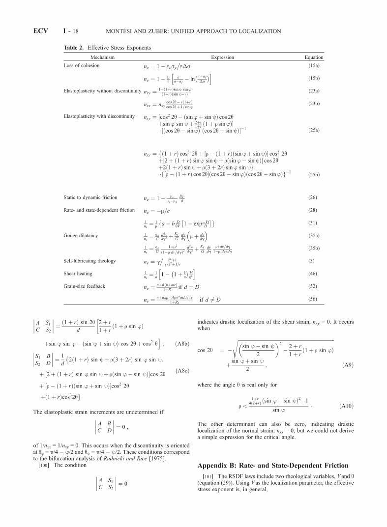
A S1C S2

¼ 1þ rð Þ sin 2qd

2þ r


� þsin j sin j� sin jþ sin yð Þ cos 2qþ cos2 q

i; ðA8bÞ

S1 B

S2 D

¼ 1

d2 1þ rð Þ sin yþ r 3þ 2rð Þ sin j sin y

�:

þ 2þ 1þ rð Þ sin j sin yþ r sin j� sin yð Þ½ �cos 2q

þ r� 1þ rð Þ sin jþ sin yð Þ½ �cos2 2q

ðA8cÞ

þ 1þ rð Þcos32q!

The elastoplastic strain increments are undetermined if

A B

C D

¼ 0 ;

of 1/nxx = 1/nxy = 0. This occurs when the discontinuity is orientedat qj = p/4 � j/2 and qy = p/4 � y/2. These conditions correspondto the bifurcation analysis of Rudnicki and Rice [1975].[100] The condition

A S1C S2

¼ 0

indicates drastic localization of the shear strain, nxy = 0. It occurswhen

cos 2q ¼ �

ffiffiffiffiffiffiffiffiffiffiffiffiffiffiffiffiffiffiffiffiffiffiffiffiffiffiffiffiffiffiffiffiffiffiffiffiffiffiffiffiffiffiffiffiffiffiffiffiffiffiffiffiffiffiffiffiffiffiffiffiffiffiffiffiffiffiffiffiffiffiffiffiffiffiffiffiffiffiffi�sin j� sin y

2

�2

� 2þ r


s

þ sin jþ sin y2

; ðA9Þ

where the angle q is real only for

r <1þr

4 2þrð Þ sin j� sin yð Þ2�1

sin j� ðA10Þ

The other determinant can also be zero, indicating drasticlocalization of the normal strain, nxx = 0, but we could not derivea simple expression for the critical angle.

Appendix B: Rate- and State-Dependent Friction

[101] The RSDF laws include two rheological variables, V and q(equation (29)). Using V as the localization parameter, the effectivestress exponent is, in general,

Table 2. Effective Stress Exponents

Mechanism Expression Equation

Loss of cohesion ne ¼ 1� ecsy�e�s (15a)

ne ¼ 1� ece

ss�sf

� lns�sf�s

� �h i(15b)

Elastoplasticity without discontinuity nxy ¼ 1þ 1þrð Þsiny sinj1þrð Þ siny�vð Þ

(23a)

nxx ¼ nxycos 2q� v 1þrð Þcos 2qþ 1=sinj

(23b)

Elastoplasticity with discontinuity nxy ¼ cos2 2q� sinjþ sinyð Þ cos 2q½þsinj sinyþ 2þr

1þr1þ r sinjð Þ�

� cos 2q� sinjð Þ½ cos 2q� sinyð Þ��1 ð25aÞ

nxx ¼ 1þ rð Þ cos3 2q�

þ r� 1þ rð Þ sinjþ sinyð Þ½ � cos2 2qþ 2þ 1þ rð Þ sinj sinyþ r sinj� sinyð Þ½ � cos 2qþ2 1þ rð Þ sinyþ r 3þ 2rð Þ sinj sinyg�f r� 1þ rð Þ cos 2q½ � cos 2q� sinjð Þ cos 2q� sinjð Þg�1 ð25bÞ

Static to dynamic friction ne ¼ 1� msms�md

DC

d(26)

Rate- and state-dependent friction ne ¼ �m=c (28)

1ne¼ 1

m a� b DqV 1� exp�Vt

D

# $� !(31)

Gouge dilatancy 1ne¼ se

Gd2vdg2

þ Kf

Gdvdg

mþ dvdg

� �(35a)

1ne¼ se

G1þm2

1�m dv=dgð Þ2d2vdg2

þ Kf

Gdvdg

mþdv=dg1�m dv=dg

(35b)

Self-lubricating rheology ne ¼ g�

_e2þ1g=_e2þ1=r

(3)

Shear heating 1ne¼ 1

n1� 1þ 1

n

� �Hq2

ih(46)

Grain-size feedback ne ¼ nþR pþmrð Þ1þR

if d ¼ D (52)

ne ¼ nþR0p�ADsnmLt=eT1þR0

if d 6¼ D (56)


1

ne¼ V

m@m@V

þ @m@q

dqdV

� �¼ 1

maþ b

V

qdqdV

� �� ðB1Þ

[102] As q is an integral function of the velocity history(equations (30a) and (30b)), the effective stress exponent dependson time and on the specific q-V history. We consider two specificcases. In the first (section 6.1), q remains at equilibrium qo = D/V,which corresponds to the limit t ! 1 or D ! 0. In that case,

dq=dV ¼ �q=V ; ðB2Þ

1=ne ¼ a� bð Þ=m ¼ c=m � ðB3Þ

In the other case (section 6.2) the system is initially at equilibriumat velocity V and q = D/V, but for t > 0, the sliding velocity is V +dV. As the velocity does not depend on time for t > 0, the stateevolution laws (equations (30a) and (30b)) can be integrated andgive

Dieterich law q ¼ D

V þ dVþ x

DdV

V V þ dVð Þ ; ðB4aÞ

Ruina law q ¼ D

V þ dV1þ dV

V

� �x

; ðB4bÞ

with x = exp[�t(V + dV )/D] For dV � V both evolution laws give

dqdV

� D

V�1þ exp �Vt

D

� �� ; ðB5Þ

which, substituted in (B1), gives (31).

[103] Acknowledgments. We thank Oded Aharonson, Mark Behn,Muriel Gerbault, Brad Hager, Greg Hirth, Chris Marone, Jim Rice, JackWisdom, and Wenlu Zhu for sharing their insight on the various physicalprocesses included in this study and Paul Tackley and Alexei Poliakov fortheir reviews. We are particularly indebted to David Bercovici, who wentwell beyond the call of duty to help us clarify the paper. Supported byNASA grant NAG5-4555.

ReferencesAnderson, E. M., The dynamics of faulting, Trans. Edinburgh Geol. Soc., 8,387–402, 1905.

Anderson, E.M., The Dynamics of Faulting and Dike Formation, Oliverand Boyd, White Plains, N. Y., 1951.

Antonellini, M. A., A. Aydin, and D. D. Pollard, Microstructure of defor-mation bands in porous sandstones at Arches National Park, Utah, J.Struct. Geol., 16, 941–959, 1994.

Bai, Y., and B. Dodd, Adiabatic Shear Localization: Occurrences, The-ories, and Applications, Pergamon, New York, 1992.

Beach, A., Retrogressive metamorphic processes in shear zones with specialreference to the Lewisian complex, J. Struct. Geol., 2, 257–263, 1980.

Beaumont, C., and G. Quinlan, A geodynamic framework for interpretingcrustal-scale seismic-reflectivity patterns in compressional orogens, Geo-phys. J. Int., 116, 754–783, 1994.

Beekman, F., J. M. Bull, S. Cloetingh, and R. A. Scrutton, Crustal faultreactivation facilitating lithospheric folding/buckling in the central indianocean, in Modern Developments in Structural Interpretation, Validationand Modelling, edited by P. G. Buchananand D. A. Nieuwland, Geol.Soc. Spec. Publ., 99, 251–263, 1996.

Bercovici, D., A simple model of plate generation from mantle flow, Geo-phys. J. Int., 114, 635–650, 1993.

Bercovici, D., A source-sink model of the generation of plate tectonics fromnon-Newtonian mantle flow, J. Geophys. Res., 100, 2013–2030, 1995.

Bercovici, D., Generation of plate tectonics from lithosphere-mantle flowand void-volatile self-lubrication, Earth Planet. Sci. Lett., 154, 139–151,1998.

Bercovici, D., Y. Ricard, and M. A. Richards, The relation between mantledynamics and plate tectonics: A primer, in The History and Dynamics of

Global Plate Motions, Geophys. Monogr. Ser., vol. 121, edited by M. A.Richards, R. G. Gordon, and R. D. van der Hilst, pp. 1–46, AGU,Washington D. C., 2000.

Bercovici, D., Y. Ricard, and G. Schubert, A two-phase model for compac-tion and damage, 1, General theory, J. Geophys. Res., 106, 8887–8906,2001a.

Bercovici, D., Y. Ricard, and G. Schubert, A two-phase model for compac-tion and damage, 3, Applications to shear localization and plate bound-ary, J. Geophys. Res., 106, 8925–8940, 2001b.

Blanpied, M. L., D. A. Lockner, and J. D. Byerlee, An earthquake mechan-ism based on rapid sealing of faults, Nature, 358, 574–576, 1992.

Blanpied, M. L., C. J. Marone, D. A. Lockner, J. D. Byerlee, and D. P.King, Quantitative measure of the variation in fault rheology due to fluid-rock interactions, J. Geophys. Res., 103, 9691–9712, 1998.

Brace, W. F., and D. L. Kohlstedt, Limits on lithospheric stress imposed bylaboratory measurements, J. Geophys. Res., 85, 6248–6252, 1980.

Branlund, J., K. Regenauer-Lieb, and D. A. Yuen, Fast ductile failure ofpassive margins from sediment loading, Geophys. Res. Lett., 25, 1989–1992, 2000.

Braun, J., J. Chery, A. N. B. Poliakov, D. Mainprice, A. Vauchez, A.Tommasi, and M. Daignieres, A simple parameterization of strain loca-lization in the ductile regime due to grain size reduction: A case study forolivine, J. Geophys. Res., 104, 25,167–25,181, 1999.

Brodie, K. H., and E. H. Rutter, On the relationship between deformationand metamorphism, with special reference to the behavior of basic rocks,in Metamorphic Reactions; Kinetics, Textures, and Deformation, Adv.Phys. Geochem., vol. 4, edited by A. B. Thompson and R. C. Rubie,pp. 138–179, Springer-Verlag, New York, 1985.

Brown, M., and G. S. Solar, Shear-zone systems and melts: Feedbackrelations and self-organization in orogenic belts, J. Struct. Geol., 20,211–227, 1998.

Brun, J.-P., and P. R. Cobbold, Strain heating and thermal softening incontinental shear zones: A review, J. Struct. Geol., 2, 149–158, 1980.

Buck, W. R., Comments on ‘‘origin of regional, rooted low-angle normalfaults’’ by A. Yin, Tectonics, 9, 545–546, 1990.

Buck, W. R., and A. N. B. Poliakov, Abyssal hills formed by stretchingoceanic lithosphere, Nature, 392, 272–275, 1998.

Burg, J.-P., Ductile structures and instabilities: Their implications for Var-iscan tectonics in the Ardennes, Tectonophysics, 309, 1–25, 1999.

Caristan, Y., The transition from high temperature creep to fracture inMaryland Diabase, J. Geophys. Res., 87, 6781–6790, 1982.

Carlslaw, H. S., and J. C. Jaeger, Conduction of Heat in Solids, 2nd ed.,Oxford Univ. Press, New York, 1959.

Comer, R. P., S. C. Solomon, and J. W. Head III, Mars: Thickness of thelithosphere from the tectonic response to volcanic loads, Rev. Geophys.,21, 61–92, 1985.

Cook, N. G. W., Stiff testing machines, stick slip sliding, and the stability ofrock deformation, in Mechanical Behavior of Crustal Rocks, Geophys.Monogr. Ser., vol. 24, edited by N. L. Carter et al., pp. 93–102, AGU,Washington, D. C., 1981.

Dahlen, F. A., and J. Supp, Mechanics, growth, and erosion of mountainbelts, in Processes in Continental Lithospheric Deformation, edited byS. P. Clark Jr., B. C. Burchfield, and J. Suppe, Spec. Pap. Geol. Soc.Am., 218, 161–178, 1988.

Dieterich, J. H., Time-dependent friction in rocks, J. Geophys. Res., 77,3691–3697, 1972.

Dieterich, J. H., Time-dependent friction and the mechanics of stick-slip,Pure Appl. Geophys., 116, 790–806, 1978.

Dieterich, J. H., Modeling of rock friction, 1, Experimental results andconstitutive equations, J. Geophys. Res., 84, 2161–2168, 1979.

Dieterich, J. H., Earthquake nucleation on faults with rate- and state-depen-dent strength, Techtonophysics, 322, 115–134, 1992.

Dimanov, A., G. Dresen, and R. Wirth, High-temperature creep of partiallymolten plagioclase aggregates, J. Geophys. Res., 103, 9651–9664, 1998.

Drucker, D. C., A more fundamental approach to plastic stress-strain rela-tions, Proc. U.S. Natl. Conf. Appl. Mech., 1st, 487–491, 1952.

Drucker, D. C., A definition of stable inelastic material, J. Appl. Mech., 26,101–106, 1959.

Edmond, J. M., and M. S. Paterson, Volume changes during the deforma-tion of rocks at high pressures, Int. J. Rock Mech. Mining Sci. Geomech.Abstr., 9, 161–182, 1972.

Evans, B., and D. L. Kohlstedt, Rheology of rocks, in Rock Physics andPhase Relations: A Handbook of Physical Constants, AGU Ref. Shelf,vol. 3, edited by T. J. Ahrens, pp. 148–165, AGU, Washington, D. C.,1995.

Fischer, G. J., and M. S. Paterson, Dilatancy during the deformation ofrocks at high temperatures and pressures, J. Geophys. Res., 94, 17,607–17,617, 1989.

Fitz Gerald, J. D., and H. Stunitz, Deformation of granitoids at low meta-morphic grade, I, Reactions and grain size reduction, Tectonophysics,221, 269–297, 1993.


Fleitout, L., and C. Froideveau, Thermal and mechanical evolution of shearzones, J. Struct. Geol., 2, 159–164, 1980.

Frank, F. C., On dilatancy in relation to seismic sources, Rev. Geophys., 3,485–503, 1965.

Froideveau, C., and G. Schubert, Plate motion and structure of the conti-nental asthenosphere: A realistic model of the upper mantle, J. Geophys.Res., 80, 2553–2564, 1975.

Gerbault, M., A. N. B. Poliakov, and M. Daignieres, Prediction of faultingfrom the theories of elasticity and plasticity: What are the limits?, J.Struct. Geol., 20, 301–320, 1998.

Gleason, G. C., and J. Tullis, A flow law for dislocation creep of quartzaggregates determined with the molten salt cell, Tectonophysics, 247, 1–23, 1995.

Gordon, R. G., Diffuse oceanic plate boundaries: Strain rates, verticallyaveraged rheology, and comparisons with narrow plate boundaries andstable interiors, in The History and Dynamics of Global Plate Motions,Geophys. Monogr. Ser., vol. 121, edited by M. A. Richards, R. G. Gordon,and R. D. van der Hilst, pp.143–159, AGU, Washington, D. C., 2000.

Griggs, D., and J. Handin, Observations on fracture and a hypothesis ofearthquakes, in Rock Deformation, edited by D. Griggs and J. Handin,Mem. Geol. Soc. Am., 79, 347–364, 1960.

Gu, J.-C., J. R. Rice, A. Ruina, and S. T. Tse, Slip motion and stability of asingle degree of freedom elastic system with rate and state dependentfriction, J. Mech. Phys. Solids, 32, 167–196, 1984.

Gu, Y., and T.-f. Wong, Non-linear dynamics of the transition from stablesliding to cyclic stick-slip in rock, in Nonlinear Dynamics and Predict-ability of Geophysical Phenomena, Geophys. Monogr. Ser., vol. 83,edited by W. I. Newman, A. Gabrielov, and D. L. Turcotte, pp. 15–35,AGU, Washington, D. C., 1994.

Hafner, W., Stress distributions and faulting, Geol. Soc. Am. Bull., 62, 373–398, 1951.

Handy, M. R., Deformation regimes and the rheological evolution of faultzones in the lithosphere: The effects of pressure, temperature, grain sizeand time, Tectonophysics, 163, 119–152, 1989.

Hill, R., The Mathematical Theory of Plasticity, Clarendon, Oxford, Eng-land, 1950.

Hill, R., A general theory of uniqueness and stability in elastic-plasticsolids, J. Mech. Phys. Solids, 6, 236–249, 1958.

Hobbs, B. E., A. Ord, and C. Teyssier, Earthquakes in the ductile regime?,Pure Appl. Geophys., 124, 309–336, 1986.

Hobbs, B. E., H.-B. Muhlhaus, and A. Ord, Instability, softening and loca-lization of deformation, in Deformation Mechanisms, Rheology and Tec-tonics, edited by R. J. Knipe and E. H. Rutter, Geol. Soc. Spec. Publ., 54,143–165, 1990.

Issen, K. A., and J. W. Rudnicki, Theory of compaction bands in porousrocks, Phys. Chem. Earth, Part A, 26, 95–100, 2001.

Jaroslow, G. E., G. Hirth, and H. J. B. Dick, Abyssal peridotite my-lonites: Implications for grain-size sensitive flow and strain localiza-tion in the oceanic lithosphere, Tectonophysics, 256, 17–37, 1995.

Jin, D., S.-I. Karato, and M. Obata, Mechanisms of shear localization inthe continental lithosphere: Inference from the deformation microstruc-tures from the Ivrea zone, northwest Italy, J. Struct. Geol., 20, 195–209, 1998.

Kameyama, M., D. A. Yuen, and H. Fujimoto, The interaction of viscousheating with grain-size dependent rheology in the formation of localizedslip zones, Geophys. Res. Lett., 24, 2523–2526, 1997.

Karato, S.-I., M. Paterson, and J. Fitz Gerald, Rheology of synthetic olivineaggregates: Influence of grain size and water, J. Geophys. Res., 91,8151–8176, 1986.

Lachenbruch, A., Frictional heating, fluid pressure, and the resistance tofault motion, J. Geophys. Res., 85, 6097–6112, 1980.

Lavier, L. L., W. R. Buck, and A. N. B. Poliakov, Self-consistent rolling-hinge model for the evolution of large-offset low-angle normal faults,Geology, 27, 1127–1130, 1999.

Lin, J., and E. M. Parmentier, A finite amplitude necking model of rifting inbrittle lithosphere, J. Geophys. Res., 95, 4909–4923, 1990.

Lockner, D. A., Rock failure, in Rock Physics and Phase Relations: AHandbook of Physical Constants, AGU Ref. Shelf, vol 3, edited by T.J. Ahrens, pp. 127–147, AGU, Washington, D. C., 1995.

Lubliner, J., Plasticity Theory, Macmillan, Old Tappan, N. J., 1990.Mackwell, S. J., M. E. Zimmerman, and D. L. Kohlstedt, High temperaturedeformation of dry diabase with application to tectonics on Venus,J. Geophys. Res., 103, 975–984, 1998.

Mandel, J., Conditions de stabilite et postulat de Drucker, in Rheology andSoil Mechanics, edited by J. Kravtchenko and P. M. Sirieys, pp. 58–68,Springer-Verlag, New York, 1966.

Mandl, G., Mechanics of Tectonic Faulting, Dev. Struct. Geol., vol. 1,Elsevier Sci., New York, 1988.

Marone, C. J., Laboratory-derived friction law and their application toseismic faulting, Annu. Rev. Earth Planet. Sci., 26, 643–696, 1998.

Marone, C. J., C. B. Raleigh, and C. H. Scholz, Frictional behavior andconstitutive modeling of simulated gouge, J. Geophys. Res., 95, 7007–7025, 1990.

McKenzie, D. P., The generation and compaction of partially molten rock,J. Petrol., 25, 713–765, 1984.

Melosh, H. J., Plate motion and thermal instability in the asthenosphere,Tectonophysics, 35, 363–390, 1976.

Melosh, H. J., and C. A. Williams, Mechanics of graben formation incrustal rocks: A finite-element analysis, J. Geophys. Res., 94, 13,961–13,973, 1989.

Montesi, L. G. J., Localization instability and the origin of regularly-pacedfaults in planetary lithospheres, Ph.D. thesis, 296 pp., Mass. Inst. ofTechnol., Cambridge, 2002.

Montesi, L. G. J., C. J. Marone, G. Hirth, and S. L. Karner, Frictionalproperties and microstructure of simulated diabase gouge at temperaturesup to 400�C, Eos Trans, AGU, 80(46), Fall Meet. Suppl., F689, 1999.

Needleman, A., and V. Tvegaard, Analyses of plastic flow localization inmetals, Appl. Mech. Rev., 45, S3–S18, 1992.

Newman, J., W. M. Lamb, M. R. Drury, and R. L. M. Vissers, Deformationprocesses in a peridotite shear zone: Reaction-softening by a H2O-defi-cient, continuous net transfer reaction, Tectonophysics, 303, 193–222,1999.

Ode, H., Faulting as a velocity discontinuity in plastic deformation, Mem.Geol. Soc. Am., 79, 293–321, 1960.

Olsson, W. A., Theoretical and experimental investigation of compactionbands in porous rock, J. Geophys. Res., 104, 7219–7228, 1999.

Orowan, E., Dilatancy and the seismic focal mechanism, Rev. Geophys., 4,395–404, 1966.

Paterson, M. S., Experimental Rock Deformation-The Brittle Field, Spring-er-Verlag, New York, 1978.

Poirier, J.-P., Shear localization and shear instability in materials in theductile field, J. Struct. Geol., 2, 135–142, 1980.

Poliakov, A. N. B., H. J. Herrman, Y. Y. Podladchikov, and S. Roux, Fractalplastic shear bands, Fractals, 2, 567–581, 1994.

Rabinowicz, E., The nature of the static and kinetic coefficients of friction,J. Appl. Phys., 22, 1373–1379, 1951.

Ramsay, J. G., Shear zone geometry, a review, J. Struct. Geo., 2, 83–99,1980.

Ranalli, G., Rheology of the Earth, 2nd ed., Chapman and Hall, New York,1995.

Regenauer-Lieb, K., Dilatant plasticity applied to the Alpine collision:Ductile void growth in the intrapate area beneath the Eifel volcanic field,Geodynamics, 27, 1–21, 1999.

Regenauer-Lieb, K., and J.-P. Petit, Cutting of the European continentallithosphere: Plasticity theory applied to the present Alpine collision, J.Geophys. Res., 102, 7731–7746, 1997.

Regenauer-Lieb, K., and D. A. Yuen, Rapid conversion of elastic energyinto plastic shear heating during incipient necking of the listhosphere,Geophys. Res. Lett., 24, 2737–2740, 1998.

Reynolds, O., On the dilatancy of media composed of rigid particles incontact, Philos. Mag., 20, 469–481, 1885.

Rice, J. R., On the stability of dilatant hardening for saturated rock masses,J. Geophys. Res., 80, 1531–1536, 1975.

Rice, J. R., The localization of plastic deformation, in Theoretical andApplied Mechanics, edited by W. T. Koiter, pp. 207–220, North-Holland,New York, 1976.

Rubie, D. C., Reaction-enhanced ductility: The role of solid-solid univar-iant reactions in deformation of the crust and mantle, Tectonophysics, 96,331–352, 1983.

Rudnicki, J. W., The stabilization of slip on a narrow weakening fault zoneby coupled deformation-pore fluid diffusion, Bull. Seismol. Soc. Am., 69,1011–1026, 1979.

Rudnicki, J. W., and C.-H. Chen, Stabilization of a rapid frictional slip on aweakening fault by dilatant hardening, J. Geophys. Res., 83, 4745–4757,1988.

Rudnicki, J. W., and J. R. Rice, Conditions for the localization of deforma-tion in pressure-sensitive dilatant materials, J. Mech. Phys. Solids, 23,371–394, 1975.

Ruina, A. L., Slip instability and state variable friction laws, J. Geophys.Res., 88, 10,359–10,370, 1983.

Rutter, E. H., On the relationship between the formation of shear zones andthe form of the flow law for rocks undergoing dynamic recrystallization,Tectonophysics, 303, 147–158, 1999.

Scholz, C. H., The Mechanics of Earthquakes and Faulting, CambridgeUniv. Press, New York, 1990.

Scholz, C. H., Evidence for a strong San Andreas Fault, Geology, 28, 163–166, 2000.

Schott, B., D. A. Yuen, and H. Schmeling, Viscous heating in heteroge-neous media as applied to the thermal interaction between the crust andmantle, Geophys. Res. Lett., 26, 513–516, 1999.


Schultz, R. A., and M. T. Zuber, Observations, models, and mechanisms offailure of surface rocks surrounding planetary surface loads, J. Geophys.Res., 99, 14,691–14,702, 1994.

Segall, P., and J. R. Rice, Dilatancy, compaction, and slip instability of afluid-infiltrated fault, J. Geophys. Res., 100, 22,155–22,171, 1995.

Shaw, B. E., Frictional weakening and slip complexity in earthquake faults,J. Geophys. Res., 100, 18,239–18,251, 1995.

Sibson, R. H., Interaction between temperature and pore fluid during earth-quake faulting and a mechanism for partial or total stress relief, Nature,243, 66–68, 1973.

Sibson, R. H., Fault rocks and fault mechanisms, J. Geol. Soc. London, 133,191–213, 1977.

Sibson, R. H., Transient discontinuities in ductile shear zones, J. Struct.Geol., 2, 165–171, 1980.

Sibson, R. H., An assessment of field evidence for ‘‘Byerlee’’ friction, PureAppl. Geophys., 142, 645–662, 1994.

Simpson, C., Borrego Springs-Santa Rosa mylonite zone: A late Cretaceouswest-directed thrust in southern California, Geology, 12, 8–11, 1984.

Sleep, N. H., and M. L. Blanpied, Ductile creep and compaction: A me-chanism for transiently increasing fluid pressure in mostly sealed faultzones, Pure Appl. Geophys., 143, 9–40, 1994.

Smith, R. B., Formation of folds, boudinage, and mullions in non-New-tonian materials, Geol. Soc. Am. Bull., 88, 312–320, 1977.

Spiegelman, M., Flow in deformable media, part 1, Simple analysis, J.Fluid Mech., 247, 17–38, 1993.

Tackley, P. J., Self-consistent generation of tectonic plates in three-dimen-sional mantle convection, Earth Planet. Sci. Lett., 157, 9–22, 1998.

Tackley, P. J., Mantle convection and plate tectonics: Toward an integratedphysical and chemical theory, Science, 288, 2002–2007, 2000.

Tapponnier, P., and P. Molnar, Slip-line field theory and large-scale con-tinental tectonics, Nature, 264, 319–324, 1976.

Tullis, J., L. Dell’Angelo, and R. A. Yund, Ductile shear zones from brittleprecursors in feldspathic rocks: The role of dynamic recrystallization, inThe Brittle-Ductile Transition in Rocks, Geophys. Monogr. Ser., vol. 56,edited by A. G. Duba et al., pp. 67–82, AGU, Washington D. C., 1990.

van der Wal, D., P. Chopra, M. Drury, and J. F. Gerald, Relationshipsbetween dynamically recrystallized grain size and deformation conditionsin experimentally deformed olivine rocks, Geophys. Res. Lett., 20, 1479–1482, 1993.

Vermeer, P. A., The orientation of shear bands in biaxial tests, Geotechni-que., 40, 223–236, 1990.

Vermeer, P. A., and R. de Borst, Non-associated plasticity for soils, concreteand rock, Heron, 29, 1–63, 1984.

Weissel, J. K., R. N. Anderson, and C. A. Geller, Deformation of the Indo-Australian plate, Nature, 287, 284–291, 1980.

White, S. H., and R. J. Knipe, Transformation and reaction-enhanced duc-tility in rocks, J. Geol. Soc. London, 165, 513–516,1978.

Whitehead, J. A., and R. F. Gans, A new, theoretically tractable earthquakemodel, Geophys. J. R. Astron. Soc., 39, 11–28, 1974.

Wittlinger, G., P. Tapponnier, G. Poupinet, M. Jiang, D. Shi, G. Herquel,and F. Masson, Tomographic evidence for localized lithospheric shearalong the Altyn Tagh fault, Science, 282, 74–76, 1998.

Wong, T., P. Baud, and E. Klein, Localized failure modes in a compactantporous rock, Geophys. Res. Lett., 28, 2521–2524, 2001.

Zhong, S., and M. Gurnis, Interaction of weak faults and non-Newtonianrhelogy produces plate tectonics in a 3D model of mantle flow, Nature,383, 245–247, 1996.

Zoback, M. D., M. L. Zoback, V. Mount, J. Suppe, J. P. Eaton, and J. H.Healy, New evidence on the state of stress of the San Andreas Faultsystem, Science, 238, 1105–1111, 1987.

Zuber, M. T., Wrinkle ridges, reverse faulting, and the depth of penetra-tion of lithospheric strain in Lunae Planum, Mars, Icarus, 114, 80–92,1995.

��L. G. J. Montesi and M. T. Zuber, Department of Earth, Atmospheric, and

Planetary Sciences, Massachusetts Institute of Technology, Cambridge, MA02139, USA. ([email protected]; [email protected])


A unified description of localization for application to large-scale tectonics

Documents

Transcript of A unified description of localization for application to large-scale tectonics