A unified approach to the generation of semantic cues for sports video annotation

ARTICLE IN PRESS

0165-1684/$ - se

doi:10.1016/j.sig

�CorrespondiE-mail addre

(W.J. Christma1Now at Visi

tion, 201 Wash

5300, USA.2Now at Silv

Balmain, 2041,

Signal Processing 85 (2005) 357–383

www.elsevier.com/locate/sigpro

A unified approach to the generation of semantic cues forsports video annotation

K. Messer, W.J. Christmas�, E. Jaser, J. Kittler,B. Levienaise-Obadia1, D. Koubaroulis2

Centre for Vision, Speech and Signal Processing, University of Surrey, Guildford GU2 7XH, UK

Received 1 August 2002; received in revised form 1 March 2003

Abstract

The use of video and audio features for automated annotation of audio-visual data is becoming widespread. A major

limitation of many of the current methods is that the stored indexing features are too low-level—they relate directly to

properties of the data. In this work we apply a further stage of processing that associates the feature measurements with

real-world objects or events. The outputs, which we call ‘‘cues’’, are combined to enable us to compute directly the

probability of the object being present in the scene. An additional advantage of this approach is that the cues from

different types of features are presented in a homogeneous way.

r 2004 Elsevier B.V. All rights reserved.

Keywords: Video summarisation; Video annotation

1. Introduction

The ever increasing popularity of sport meansthat there is a vast amount of sports footage beingrecorded every day. Ideally, all this sports video

e front matter r 2004 Elsevier B.V. All rights reserve

pro.2004.10.008

ng author.

ss: [email protected]

s).

on Technologies Laboratory, Sarnoff Corpora-

ington Road, CN 5300, Princeton NJ 08553-

erbrook Research Pty Ltd., 393 Darling St.,

NSW, Australia.

should be annotated, and the meta-data generatedon it should be stored in a database along with thevideo data. Such a system would allow an operatorto retrieve any shot or important event within ashot at a later date. Also, the level of annotationprovided by the system should be adequate tofacilitate simple text-based queries. Such a systemhas many uses, for example in the production oftelevision sport programmes and documentaries,and in ensuring the preservation of our culture.Due to the large amount of material being

generated, manual annotation is both imprac-tical and very expensive. However, automatic

d.

www.elsevier.com/locate/sigpro

ARTICLE IN PRESS

K. Messer et al. / Signal Processing 85 (2005) 357–383358

annotation is a very demanding and an extremelychallenging computer vision task as it involveshigh-level scene interpretation.Perhaps the most well known automatic video

annotation system reported in the literature isVirage [35]. Virage has an open framework whichallows for the integration of many audio and videoanalysis tools in real time and places the data intoan industry-standard database such as Informix orOracle. However, the number of analysis toolsavailable is limited, although always expanding.The main problem with Virage is that no effort hasbeen made to bridge the gap between theinformation provided by the low-level analysistools and the high-level interpretation of the video,which is required for our application.The work of Saur et al. [28] is specific to some

form of sports annotation, including the use ofcamera motion to help in the automatic annotationof basketball. Mo et al. utilise state transitionmodels, which include both top-down and bottom-up processes, to recognise different objects in sportsscenes [21]. In [16] work has been undertaken todistinguish between sports and non-sports MPEGcompressed video. Finally, MIT have been workingon the analysis of American football video [12].Several authors report a three-stage approach to

semantic annotation, in contrast to the usualapproach of some type of classifier applied to theoutput of a set of feature detectors (e.g. theBayesian network approach of [34]). In Qian et al.[25] the authors describe a three-level approach tosemantic event detection. The three levels roughlycorrespond to the feature detection, cue detectionand final classification stages of our method. Forthe low-level features they use texture and colouranalysis, together with simple global and objectmotion features. In contrast to our method, in theintermediate level, a single neural-net-based meth-od incorporates all of the low-level features togenerate a low-level semantic annotation for thewhole shot. Also, in their method, hard decisionsare made at the intermediate level.In Naphade et al. [22], a three-level approach is

also employed. The intermediate-level stage (whichgenerates data structures called ‘‘multijects’’)exploits temporal context by the use of a develop-ment of hidden Markov models. Also they express

the output of this stage in a probabilistic sense,although a hard decision is made about thepresence or otherwise of the multijects. Thistechnique is developed in Naphade and Huang[23]. Here the authors use spatio-temporal seg-mentation to identify regions of consistent fea-tures. In the final stage they use a Bayesiannetwork to generate higher-level semantic annota-tion from the multijects.The ASSAVID project [1] is concerned with the

development of a novel system which will generatesemantic annotation of sports audio-visual materi-al. This annotation segments the sports video intosemantic categories (e.g. type of sport, eventwithin the sport) and permits the user to formulatequeries to retrieve events that are significant tothat particular sport. ASSAVID will provide thecomplete system. The engine will consist of a set ofsoftware tools to aid an operator in the generationof the high-level annotation for incoming sportsvideo. These tools are based on a set of lower-levelaudio and video analysis tools, which we term cuedetectors. A contextual reasoning engine will thenbe used to analyse the output of these cue detectorsand attach semantic information to the videobeing analysed. The generated meta-data andvideo data will then be stored in a database whichis based on a mixture of IBM’s Media360 andInformix. ASSAVID will also provide a Javagraphical user interface to the database which willallow the user to browse the video, view sequencesand generate story boards, formulate queries andanalyse and modify the generated indices.In this paper we also present a three-stage

approach to semantic annotation. In this work, theoutput of the intermediate level is what we term‘‘cues’’. Each cue detector can be broken downinto two parts: a conventional feature detector,and a classifier. The feature detector providesfeatures of for example colour, texture, motioncontent, or audio spectrum. The classifier is thentrained, using the features from a specific detectoras input, to recognise real-world concepts such asgrass, weight-lifter, etc., which we denote as cues.Each cue detector presents its output in aconsistent manner, regardless of the type of featuredetector or classifier; this enables disparate cues tobe combined easily for higher-level feature and

ARTICLE IN PRESS

K. Messer et al. / Signal Processing 85 (2005) 357–383 359

event detection, and is one of the strengths of theASSAVID system. The cue output is also prob-abilistic: we regard it important to avoid makinghard decisions about the presence or absence ofcues at this stage. The cue-based approach is notspecific to our project; it can readily be used inother applications by providing the relevant train-ing data (in the form of video and audio samples)and then running the existing classifier trainers.The work described in this paper describes part

of the ASSAVID project: namely the use of visualcues to determine the type of sport being played in acompilation of Olympics footage. The paper isstructured as follows. In the next section there is abrief discussion of the user requirements thatprovided the direction of the ASSAVID project. InSection 3 we develop the methodology for the cue-based approach. We describe in Section 4 the videoanalysis tools used to derive the cues, and in Section5 the classifier used to identify the sports discipline.The experiments performed to evaluate these tech-niques are presented in Section 6. Finally in Section7 we discuss our findings and present conclusions onthe cue-based approach for event detection.

2. User requirements

An investigation into the user requirements for asports annotation system was carried out withinthe Sports Department at the BBC. It was foundthat two separate logging (meta-data creation)processes are currently used when analysing thesports video and this functionality will need to beprovided by ASSAVID. These are termed produc-tion logging and posterity logging.Production logging is when there is a need to

perform some of the annotation in real time, as theevent is actually happening. This is usually due totime pressures to get a BBC sports programmemade as quickly as possible. Currently thisannotation is made manually and is mainlyfocused on marking shots for inclusion in asubsequent programme. For example, excitingfootball shots from a Saturday afternoon matchare marked for inclusion into the Saturday nightfootball highlights programme, ‘‘Match of theDay’’. As the loggers cannot stop the action while

they are writing the log there is a tendency to skipinformation, make errors and forget importantfacts. Therefore, the nature and format of theselogs make them unsuitable for use in any long-term archiving.Posterity logging is typically performed off-line,

i.e. after the event has happened. There are fewertime constraints on how quickly the annotationneeds to be built and the major aim is to get a verydetailed description of the sports video beingarchived. The higher quality this log, the moreaccurate and efficient any subsequent retrievalbecomes. Again, at present these logs are done byhand by skilled librarians. However, this approachis very time consuming. For example, it is notuncommon for a 1 h sequence to take over 10 h toindex fully.At first, ASSAVID is concerned with supporting

the posterity logging process. However, many ofthe techniques being developed for this process arecapable of running in real time, and hence will bedirectly applicable to the production logging.Many different annotation tasks for the loggingwere identified for ASSAVID, of which some ofthe more important ones are:

�
Shot change detection. � Shot description (e.g. camera movement, lenseffects and framing terms).
�
Identification and classification of sport (e.g.football, tennis, interview).
�
Event identification within sport (e.g. goals,headers, race start. red cards etc.).
�
Sports personality detection (e.g. Alan Shearer,Tim Henman).
�
Audio Descriptors (e.g. crowd cheering/booing,gunshot).
As one can see from the above list some of thesetasks require a high-level of understanding of thevideo being analysed.

3. Cue detection

3.1. Introduction

The type of information that is typicallyextracted from audio-visual data and then used

ARTICLE IN PRESS


to annotate it is the output of a set of featuredetectors. The particular feature detectors used areoften chosen because they are able to provide usefuland powerful discrimination for a wide variety ofsituations. Many of the MPEG-7 descriptors fallinto this category. However no attempt is made torelate the feature detector outputs to what we ashumans recognise in the same audio-visual materi-al. Bearing this in mind, we introduce here theconcept of a visual cue, for two reasons:

(i)
as a means of relating the outputs of thesevisual feature detectors to actual objectsappearing and events taking place in the scenethat has been recorded, and
(ii)
to enable us to relate the outputs of severalvery different feature detection methods withina single measurement framework.
Thus the process of detecting cues in a scene, usingthe output of a feature detector as the source data,can be viewed as bridging the gap between thelower-level features traditionally used for audio-visual database annotation, and semantic objects.We now develop the cue concept further,

describing in more detail what we mean by theterm ‘‘cue’’, and showing how it is implemented inpractice. In the next subsection we elaborate onthe notion of a cue, and define some of the relatedterms. In the following subsection (Section 3.3) wediscuss the generation of cue evidence from featuredetector outputs from a more theoretical perspec-tive. Finally in Section 3.4 we outline the stepsrequired for a practical implementation of cuetraining and cue evidence generation.

3.2. Cue vocabulary

What do we mean by a ‘‘cue’’? A cue is anaudio-visual event, i.e. something happening, orthe appearance of an object, at a particular timeand spatial location in the scene that has beenrecorded. Examples of cues could be: grass, sky,swimming pool lanes, referee’s whistle, sprintrunning frequency, boxing ring ropes. This con-trasts with typical feature detector outputs: tex-ture, colour histograms, periodic motion, globalmotion, all of which we use as inputs to our cuegeneration processes.

Our task is to generate evidence for the presenceof a cue in a scene, using the output of a featuredetector as data. Thus it is apparent that there alsohas to be some kind of training process, toassociate particular feature detector outputs withthe cue in question. Each feature detector can beassociated with several different cues: by theirnature feature detectors are often designed to begeneral-purpose, while the cues are typically fairlyspecific.We introduce some relevant terms:A/V data: the raw audio-visual data as decoded

from the ASSAVID DV tapes.Cue evidence: the representation, as a real value

(or pair of values), of the evidence for the presenceof a cue. The time of occurrence and (optionally,for visual cues) location within the image are alsoincluded. The representation as real values, ratherthan classifier labels, is seen as crucial: thegeneration of labels requires the use of thresholds,which in turn would discard information that weregard as valuable. The use of thresholds will bedelayed until the contextual reasoning packagethat combines the evidence for the various cues.

Cue template: a piece of A/V data (e.g. region ofan image, image sequence, audio clip) thatcontains only the cue and nothing else, used fortraining.

Classifier: an algorithm that can be trained toassociate the output from a feature detector with aparticular cue. In the context of cues, a classifiergenerates a single scalar output (normally real-valued), rather than classifying into a set ofdiscrete states.

Method: a particular feature detector, withassociated classifier, e.g. neural network colour/texture; texture codes; multimodal colour. Anindividual method may be used to generate severaldifferent cue representations, by training theclassifier to recognise different cues.

Cue detector: the software that generates the cueevidence from the A/V data.

3.3. Creating cue evidence from measurements

3.3.1. The basis

In this section we describe the mechanismwhereby evidence for the presence of cues can be

ARTICLE IN PRESS


generated from the outputs of the feature detec-tors. We assume that a feature detector method(feature detector + associated classifier) generatesa series of scalar values fmg: The classifier has beentrained separately for each relevant cue so that theoutput m discriminates between A/V data thatdoes or does not contain the cue.The objective is to use a single classifier output

measurement m to estimate the probability of thepresence of a cue C. Since the values fmg aresamples of some underlying random variable M,we can use Bayes’ rule:

PðCjmÞ ¼pðmjCÞPðCÞ

pðmjCÞPðCÞ þ pðmjCÞPðCÞ: (1)

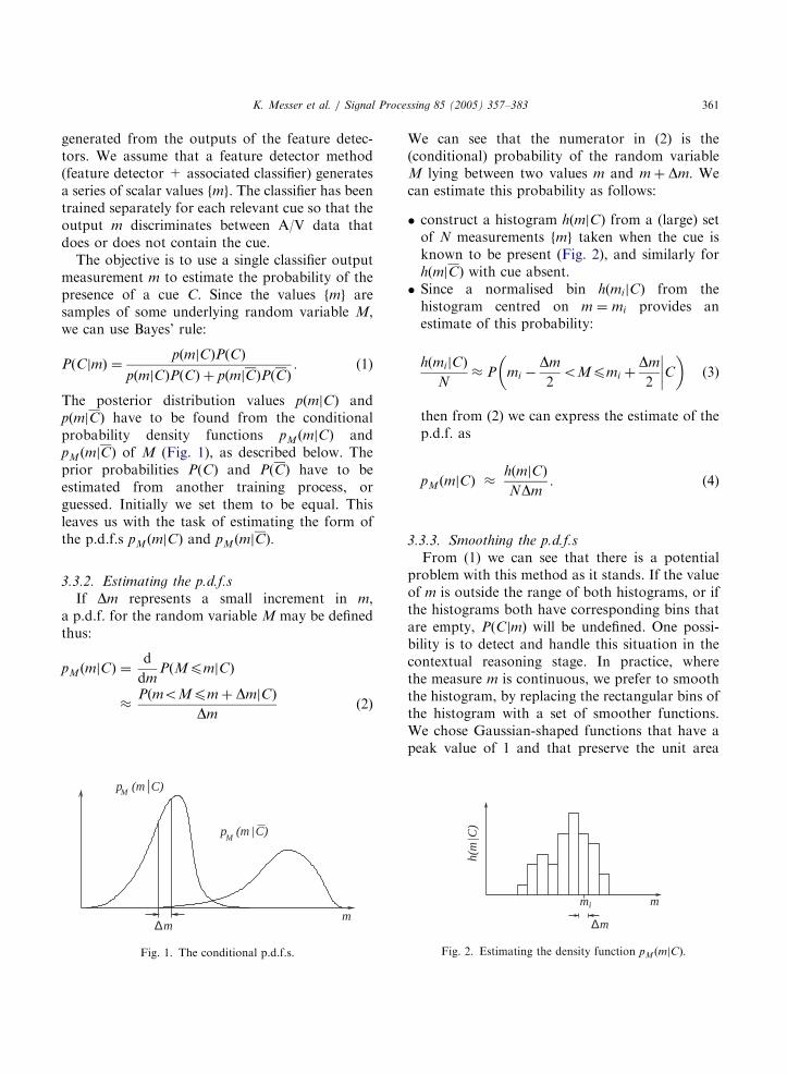
The posterior distribution values pðmjCÞ andpðmjCÞ have to be found from the conditionalprobability density functions pMðmjCÞ andpMðmjCÞ of M (Fig. 1), as described below. Theprior probabilities PðCÞ and PðCÞ have to beestimated from another training process, orguessed. Initially we set them to be equal. Thisleaves us with the task of estimating the form ofthe p.d.f.s pM ðmjCÞ and pM ðmjCÞ:

3.3.2. Estimating the p.d.f.s

If Dm represents a small increment in m,a p.d.f. for the random variable M may be definedthus:

pMðmjCÞ ¼d

dmPðMpmjCÞ

PðmoMpm þ DmjCÞ

Dmð2Þ

p (m C)M

|

p (m C)M|

m∆m

Fig. 1. The conditional p.d.f.s.

We can see that the numerator in (2) is the(conditional) probability of the random variableM lying between two values m and m þ Dm: Wecan estimate this probability as follows:

�
construct a histogram hðmjCÞ from a (large) setof N measurements fmg taken when the cue isknown to be present (Fig. 2), and similarly forhðmjCÞ with cue absent.
�
Since a normalised bin hðmijCÞ from thehistogram centred on m ¼ mi provides anestimate of this probability:
hðmijCÞ

N P mi

Dm

2oMpmi þ

Dm

2

��C� �

(3)

then from (2) we can express the estimate of thep.d.f. as

pMðmjCÞ hðmjCÞ

NDm: (4)

3.3.3. Smoothing the p.d.f.s

From (1) we can see that there is a potentialproblem with this method as it stands. If the valueof m is outside the range of both histograms, or ifthe histograms both have corresponding bins thatare empty, PðCjmÞ will be undefined. One possi-bility is to detect and handle this situation in thecontextual reasoning stage. In practice, wherethe measure m is continuous, we prefer to smooththe histogram, by replacing the rectangular bins ofthe histogram with a set of smoother functions.We chose Gaussian-shaped functions that have apeak value of 1 and that preserve the unit area

h(m

C)

|

im

m∆

m

Fig. 2. Estimating the density function pM ðmjCÞ:

ARTICLE IN PRESS


appropriate to a density function estimate. Henceour histogram estimate becomes:

hðmjCÞ ¼X

i

hðmijCÞ exp pm mi

Dm

� �2� � ;

(5)

where mi is the abscissa of the centre of the ithhistogram bin. A useful consequence of this is that,when the corresponding bins are both empty, thecue estimates will be biased in favour of the p.d.f.that has significant energy nearer to the value of m.Most of the classifiers developed (or under

development) for this project fit into the modeldescribed above. The current exception is theMNS method (Section 4.3), where the classifiergenerates an output that cannot meaningfully bemapped onto R; therefore for this method p.d.f.smoothing cannot sensibly be used.

3.4. The ‘‘generalised’’ cue evidence generation

process

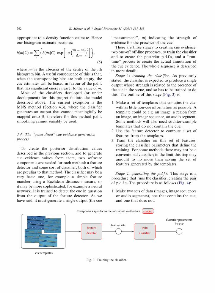
To create the posterior distribution valuesdescribed in the previous section, and to generatecue evidence values from them, two softwarecomponents are needed for each method: a featuredetector and some sort of classifier, both of whichare peculiar to that method. The classifier may be avery basic one, for example a simple featurematcher using a Euclidean distance measure, orit may be more sophisticated, for example a neuralnetwork. It is trained to detect the cue in questionfrom the output of the feature detector. As wehave said, it must generate a single output (the cue

Components specific to the

feature

detector

cue templates

Fig. 3. Training t

‘‘measurement’’, m) indicating the strength ofevidence for the presence of the cue.There are three stages to creating cue evidence:

two one-off off-line processes, to train the classifierand to create the posterior p.d.f.s, and a ‘‘run-time’’ process to create the actual annotation ofthe cue evidence. The whole sequence is describedin more detail:

Stage 1: training the classifier. As previouslystated, the classifier is expected to produce a singleoutput whose strength is related to the presence ofthe cue in the scene, and so has to be trained to dothis. The outline of this stage (Fig. 3) is:

1.

fea

in

he c

Make a set of templates that contains the cue,with as little non-cue information as possible. Atemplate could be e.g. an image, a region froman image, an image sequence, an audio segment.Some methods will also need counter-exampletemplates that do not contain the cue.

2.
Use the feature detector to compute a set offeatures from the templates.
3.
Train the classifier on this set of features,storing the classifier parameters that define thetraining. For some methods there may not be aconventional classifier; in the limit this step mayamount to no more than saving the set offeatures generated by the templates.
Stage 2: generating the p.d.f.s. This stage is aprocedure that runs the classifier, creating the pairof p.d.f.s. The procedure is as follows (Fig. 4):

1.
Make two sets of data (images, image sequencesor audio segments), one that contains the cue,and one that does not.
ture sets

dividual method are

classifier parametersfor cue

train

classifier

shaded

lassifier.

ARTICLE IN PRESS

feature setsmeasurements

cue

Components specific to the individual method are Timecodes for

images (or sequences)ground-truthed for cue

m{ }

for cueclassifier parameters

createhistograms

shaded

detector

feature

run

classifierwith cues

without cues

Fig. 4. Generating the p.d.f.s.

feature setsmeasurements

cue

Components specific to the individual method are

Timecodes forimages (or sequences)

ground-truthed for cue- if testing,

evidencecue

classifier / cueparameters

generate

valuesp.d.f.

m{ }

shaded

featuredetector

classifierrun

Fig. 5. Generating the cue evidence values.


2.
Run the feature detector and classifier on thetwo data sets, generating two sets of cuemeasurements.
3.
Generate a pair of histograms from the two setsof cue measurements. These histograms consti-tute the data used to estimate the pair of p.d.f.s.(3), (4).
Stage 3: testing/annotation. The system is nowready to generate cue evidence data. The featuredetector, classifier and cue evidence generation arerun on the test data set, using the p.d.f. pairs togenerate pairs of p.d.f. values from the classifieroutput (Fig. 5):

1.
Run the feature detector and classifier on thetest data set, generating a set of cue measure-ments.
2.
Create the cue evidence from the cue measure-ments and the p.d.f. data, in the form of a set ofp.d.f. value pairs together with any otherinformation such as time-codes, location etc.
This stage is run on this data set for all of the cuesof the various methods, as a single process. Iftesting, a further independent set of ground truthdata for the cues is needed for this stage.

3.5. Conclusions

In summary we have described a process forextracting evidence of the presence of real-worldsports-related cues from the audio-visual material.Two main processes are involved: feature extrac-tion, and evidence generation from a classifier

ARTICLE IN PRESS


process. The cue representation provides threeadvantages over a feature-based approach:

�
a more compact representation (two valuesinstead of a feature vector)
�
a unified representation (p.d.f. values instead ofdisparate feature vector values)
�
a higher-level representation
4. Visual cues

For the ASSAVID system many different cuedetection methods are being developed, includingimage-based, video-based and audio-based. In thispaper we present three image-based methods:‘‘Neural Net’’ (NN), ‘‘Texture Codes’’ (TC) and‘‘Multimodal Neighbourhood Scheme’’ (MNS).These methods all operate on images sampledfrom the video stream. Typically we sample thevideo stream at a rate of 1 frame/s. Thus the cuesrepresent the audio-visual content at a particularmoment, even though some of the future methodsthat we are developing will use local temporalinformation, for example to generate a frequencyspectrum. The wider use of the temporal context isdeferred until the contextual reasoning stage. Thissystem contrasts therefore with for example the‘‘Multiject’’ concept [22], which captures temporalcontext through the use of hidden Markov modelsat a relatively low level. In some related systems(e.g. [23]), the methods operate on segmentedimages. However we wished to avoid the need forimage segmentation, as we found it difficult toidentify a segmentation method that would re-liably generate useful segmentations throughoutthe video material. The methods used here wereselected because each of them operates globally onthe image, without the need for segmentation.In each case, the algorithm can be broken down

into two principal components: a feature detector,and a classifier or matcher stage that generates thecue measurement. There may optionally be anobject locator, which in addition to improving theclassification or matching, provides informationabout the position of the object in the image. Eachmethod can be used to form a number of different

cue detectors provided that appropriate trainingdata is available. Each of the three methods usedfor the experiments in this paper is described inturn.

4.1. Neural network-based cues using combined

colour and texture

Each neural network-based cue is a trainedneural network sensitive to that type of cue. As themethod uses both colour and texture information,in order for the cue to be useful the cue must havestrong colour and/or texture information. Cuesthat are suitable for this method include therecognition of for example athletics track, grass,sky, tennis court and swimming pools.In the rest of this subsection the colour and

texture feature descriptors employed for thismethod are described in detail and the classifierprocesses required to train and use each cue ispresented.

4.1.1. Feature extraction

Consider an image I of width c and height r forwhich a user wishes to compute a set of colour andtexture features. For every pixel pðk;lÞ in the image(apart from boundary regions) a correspondingfeature vector fðk;lÞ ¼ fy1; y2 . . . ydg of d dimensionsis computed, where 1pkpr and 1plpc: Thisfeature vector contains information about thelocal texture and colour properties in thelocal neighbourhood of pðk;lÞ: For these cuesfour different types of texture feature extractorand one colour feature extractor have beenemployed to obtain the feature measurements y1to yd : A brief summary of these are given inTable 1. A more detailed description of eachfeature extractor then follows. As one can see, foreach pixel 33 different features are computed, i.e.d ¼ 33:When training the classifier (Section 4.1.2), the

features are extracted for every pixel in thetemplate (apart from border regions). Whenrunning the classifier, the image is more coarselysampled: a Sobol sampler [6] is used, extracting1% of the pixels randomly from each image.

The discrete cosine transform: Consider the three1-dimensional DCT vectors shown in Eq. (6) of

ARTICLE IN PRESS

Table 1

Table of the four different feature extractors used to calculate

the values in the feature vector

Feature extractor Feature values Image type

Discrete cosine

transform

y1 to y9 Grey-level

Gabor transform y10 to y17 Grey-level

Wavelet transform y18 to y21 Grey-level

Intensity-based y22 to y33 Colour and

grey-level


length N ¼ 3:

u1 ¼ ½1:0; 1:0; 1:0�; u2 ¼ ½1:0; 0:0;1:0� and

u3 ¼ ½1:0;2:0; 1:0�: ð6Þ

From these, nine 3 3 masks, di; can begenerated using Eq. (7):

dið�; �Þ ¼ upð�Þ uqð�Þ; (7)

where i ¼ p þ ðq 1ÞN for 1pp; qpN: The out-put, yðk; lÞ; of channel i at image position ðk; lÞ isgiven by

yiðk; lÞ ¼XN1

a¼0

XN1

b¼0

dða þ 1; b þ 1Þ xðk a; l bÞ:

(8)

This will produce nine transformed images. Onthese images the local variance in a23 23 window is computed. The values obtainedare the feature measurements. Table 2 shows eachof the nine masks used to obtain the transformedimages. Further information on these features canbe found in [32].

Gabor filters: Gabor filters are widely used as atexture filter because of their parallel in humanphysiology. They operate as follows.First the image is transformed into the fre-

quency domain using a Fast Fourier Transform.This transformed image is then multiplied by a setof Gabor filter masks. These masks form two semi-circles of filters, spaced at 45�; covering approxi-mately one half of the 2-D frequency plane. Themasks are chosen such that the highest centrefrequency remains below the Nyquist frequencyand the support of the largest filter support iscompatible with the image size. The Gabor filtermasks are governed by four parameters: radial

centre frequency f 0; preferred orientation y0;radial frequency bandwidth Bu and the orientationbandwidth By: The filters are obtained fromEq. (9):

Gðu; vÞ ¼ exp2p2½ðu0f 0Þ

2s2xþðv0syÞ2�; (9)

where ðu0; v0Þ ¼ ðu cos y0 þ v sin y0;u sin y0 þv cos y0Þ are the rotated coordinates and

sx ¼1

f 0p

ffiffiffiffiffiffiffiffiln 2

2

rð2Bu þ 1Þ

ð2Bu 1Þ; (10)

sy ¼1

f 0p tanBy2

ffiffiffiffiffiffiffiffiln 2

2

r: (11)

Table 3 shows the values of the parameters used toobtain the filters.These filtered images are then transformed back

to the spatial domain using the inverse Fouriertransform, and the modulus of the complex pixelvalues retained. The local variance of each pixel ina sliding 23 23 window is then calculated. Theobtained values are the feature values.More information on Gabor filters can be found

in [14,3,13,31].Wavelet transform: Consider the two 1-dimen-

sional Wavelet vectors of length N ¼ 6:

h ¼ ½0:333; 0:807; 0:460;0:135;

0:085; 0:035� and ð12Þ

g ¼ ½0:035; 0:085;0:135;

0:460; 0:807;0:333�: ð13Þ

From these, four 6 6 masks, di are constructed(see Table 4). The output, y, of channel i is thengiven by the convolution of the 2-D mask di withthe image x:

yi ¼ x n di: (14)

This will produce 4 transformed images (Table4). On these images the local variance in a23 23 window is computed. These obtainedvalues are the feature measurements.More information on the wavelet transform can

be found in [7].Intensity features: These features are computed

for each of the red, green and luminance planes. A23 23 window R is slid over the image. At each

ARTICLE IN PRESS

Table 2

The nine DCT masks

dct1 ¼

1 1 1

1 1 1

1 1 1

264

375 dct2 ¼

1 0 1

1 0 1

1 0 1

264

375 dct3 ¼

1 2 1

1 2 1

1 2 1

264

375

dct4 ¼

1 1 1

0 0 0

1 1 1

264

375 dct5 ¼

1 0 1

0 0 0

1 0 1

264

375 dct6 ¼

1 2 1

0 0 0

1 2 1

264

375

dct7 ¼

1 1 1

2 2 2

1 1 1

264

375 dct8 ¼

1 0 1

2 0 2

1 0 1

264

375 dct9 ¼

1 2 1

2 4 2

1 2 1

264

375

Table 3

The eight Gabor filters

Feature f 0 y0 Bu By

gab1 0.125 0.0 1.5 45.0

gab2 0.125 45.0 1.5 45.0

gab3 0.125 90.0 1.5 45.0

gab4 0.125 135.0 1.5 45.0

gab5 0.35 0.0 1.5 45.0

gab6 0.35 45.0 1.5 45.0

gab7 0.35 90.0 1.5 45.0

gab8 0.35 135.0 1.5 45.0

Table 4

The four wavelet masks

Feature Mask

wlt1 d1 ¼ hT:hwlt2 d2 ¼ hT:gwlt3 d3 ¼ gT:hwlt4 d4 ¼ gT:g


position a histogram hðiÞ is formed. This is done,by counting the number of occurrences of eachpixel value. The normalised histogram is given byPðiÞ ¼ hðiÞ=N where N is the total number of pixelswithin the window. Four statistics are thencomputed on this histogram, creating 12 vectorcomponents in all.

�
Mean
m ¼X255i¼0

i:PðiÞ: (15)

�
Variance
s2 ¼X255i¼0

ði mÞ2:PðiÞ: (16)

�
Energy
Measures the homogeneity of the histo-gram. Takes large values when the histo-gram has a few bins largely filled and smallvalues when many bins are partially filled.

E ¼X255i¼0

PðiÞ2: (17)

�
Entropy
This is a measure of the information contentof a histogram and takes values accordingto how smooth the histogram is

H ¼X255i¼0

PðiÞ: log½PðiÞ� (18)

Further information on these intensity featurescan be found in [10].

4.1.2. The cue classifier

Training the classifier: A 33 input, five hiddenunit and single output unit neural network istrained using a ground-truthed, two class data set.The first class contains data samples computed onthe image areas containing exclusively the cue. Forexample, if the chosen cue is grass then this class

ARTICLE IN PRESS


should contain only feature vectors correspondingto grass pixels in a set of training images. Thesecond class contains feature vectors from trainingimage areas which are known not to contain pixelsof the cue of interest. This step has to be operatorguided. The network is then trained using theback-propagation algorithm [2], setting the outputto fire when a feature vector from the cue ispresented at the input and output not to fire whena feature vector from non-cue is presented.

Running the classifier: To compute the cue on atest image (e.g. keyframe) the same set of thirty-three colour and texture features are computed forpixels in the test image. Each test pixels featurevector is then presented to the trained network andthe value of the output observed. A high valueindicates that the feature vector is more similar toa feature vector from the cue. A low valueindicates non-similarity to the cue.To compute the measurement value m, intro-

duced in Section 3.3.1, the mean network outputof the pixels input feature vectors over the wholeimage is currently used, for convenience. However,other ways of combining the network outputscould be investigated.

4.2. Cues based on texture codes

Texture can be exploited as a rich source ofinformation when annotating sports images. Forinstance, the grass present on football pitches orthe water present in water-sports are both char-acterised by specific textural properties. Certaintextural descriptors, such as those we are using inthis module, have also a natural ability to describeobjects, by encoding the structural properties ofareas of the image.

texturefilter

test imageindexing/ hashing

templatetraining da

Fig. 6. The texture cue

In this module, the feature extraction consists ofa texture filter followed by an indexing module.The feature matching unit consists of two parts: acoarse matching process and a localisation process(Fig. 6). In the cue training mode, templates(regions from keyframes) are selected for each cue.These templates are analysed by the texture filterand indexing submodules, and the results stored asthe training output data. In the annotation mode,the test image is again analysed by the texture filterand indexing submodules, and the test imagetexture indices are compared with those of thecue prototype in the coarse matching process. Thelocalisation process then identifies the areas of theimage which the selected templates match mostclosely. The localisation process yields a matchconfidence for each template, and the highestconfidence is retained as a match confidence forthe cue. The components are now described inmore detail.


Texture filter: The texture codes method uses abank of Gabor filters as the basic filtering element,similar to those used in the neural net method(Section 4.1). Since this method relies exclusivelyon the Gabor filter outputs to provide its features,we include a third semi-circle of 4 filters to providebetter frequency resolution, making 12 filters in all.Each ring then has a frequency bandwidth of oneoctave.Gabor filters by themselves do not yield

illumination invariant responses; hence we nor-malise the filter outputs. We assume a linear modelfor changes in lighting condition: if I1 and I2 aretwo images differing by the lighting conditions,then I2ðx; yÞ ¼ aI1ðx; yÞ þ b: By setting to zero the

measurecue evidence

detection:

localisation

coarse detection

ta

evidence module.

ARTICLE IN PRESS


zero frequency component of the filter, we canremove the constant component b: The scalingcomponent a is then removed by normalising asfollows: at each pixel, the energy Eiðx; yÞ of the ithfilter response is divided by the average energy ofall the N filter responses at that pixel:

E0iðx; yÞ ¼

Eiðx; yÞPNj¼1Ejðx; yÞ

: (19)

Each energy response is thus weighed against thepool of all of the filter responses. This normal-isation approach has been supported by physiolo-gical research and models of texture perception[11], and its effectiveness confirmed in [18]. Theresponse is expressed as an amplitude, by takingthe square root of the response:

Tiðx; yÞ ¼ffiffiffiffiffiffiffiffiffiffiffiffiffiffiffiE0

iðx; yÞq

(20)

Finally, we linearly smooth the texture representa-tion. This step attenuates local fluctuations, andeffectively reduces the spread of the texturefeatures associated with homogeneous regions inthe texture space. Currently we use a simplerectangular averaging window of size 25 25pixels, which corresponds approximately to thesupport of the lowest-frequency filters in ourGabor set.

Indexing module: Each image is then indexed tocreate a set of compact descriptors. The texturefilter yields a 12-D feature space, where eachdimension corresponds to the normalised ampli-tude axis of one Gabor filter. We partition thisspace into fixed hypercubes, so that we can assigna ‘‘texture code’’ to any pixel in an image byconsidering in which hypercube the 12-D normal-ised energy vector obtained at that pixel falls. Thecode consists of the concatenated 12 quantisednormalised energies obtained from the filter bank,so that each pixel is associated with one corner ofthe hypercube into which it falls. Following [17],we are currently using a uniform quantisationscheme for the partitioning of the 12-D filter space.The codes are stored in two different forms:

�
as an ‘‘annotation table’’ (a hash table) for thecoarse matching. For each image associated witha given cue, we note each code found in this
image and its frequency. If the frequency isbelow a fixed threshold the code is discarded;otherwise it is added to a hash table we refer toas the ‘‘annotation table’’. This table stores thekeys (indices) of the texture codes found in thetemplate. We use a quantisation step of 0.2 forthe codes stored in the hash table.

�
as a ‘‘code image’’ for the localisation process.In order to achieve a further data reduction, wepartition the image into ð3 3Þ non-overlappingneighbourhoods and record only the codeoccurring the most frequently in each neigh-bourhood. We use a finer quantisation step of0.015 for the codes stored in the code images: thelocalisation process will be more precise withfiner codes.
This annotation table and associated code imagerepresent the detected features for this method.

4.2.2. Matching module

In the training mode, the feature detector(comprising texture filter and indexing module) isused to extract annotation tables and code imagesfrom a set of image regions (templates) thatrepresent the cue, one table and code image foreach template. These represent the training outputdata for the cue, and are stored as in effect theequivalent of the classifier parameters in the neuralnet method.In annotation (i.e. ‘‘testing’’) mode, the image

is first analysed and indexed in the same fashionas the cue templates. It is then passed to thematching submodule which performs twooperations: a coarse cue matching, and a cuelocalisation.

Coarse matching: The coarse matching processconsists in retrieving from a cue’s annotation tablethe subset of templates which are most likely to bevisually similar to an area of the image beingannotated. Such a retrieval is based on similaritymeasures which enable partial comparisons, anddue to the hashed structure of the annotationtables, this process can be quite fast. Morespecifically, the texture codes extracted from animage are looked up in the annotation tableassociated with the cue. For each code extractedfrom the image and present in the table, a list of

ARTICLE IN PRESS


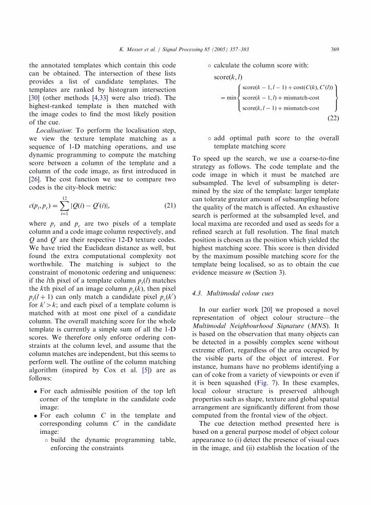
the annotated templates which contain this codecan be obtained. The intersection of these listsprovides a list of candidate templates. Thetemplates are ranked by histogram intersection[30] (other methods [4,33] were also tried). Thehighest-ranked template is then matched withthe image codes to find the most likely positionof the cue.

Localisation: To perform the localisation step,we view the texture template matching as asequence of 1-D matching operations, and usedynamic programming to compute the matchingscore between a column of the template and acolumn of the code image, as first introduced in[26]. The cost function we use to compare twocodes is the city-block metric:

cðpt; pcÞ ¼X12i¼1

jQðiÞ Q0ðiÞj; (21)

where pt and pc are two pixels of a templatecolumn and a code image column respectively, andQ and Q0 are their respective 12-D texture codes.We have tried the Euclidean distance as well, butfound the extra computational complexity notworthwhile. The matching is subject to theconstraint of monotonic ordering and uniqueness:if the lth pixel of a template column ptðlÞ matchesthe kth pixel of an image column pcðkÞ; then pixelptðl þ 1Þ can only match a candidate pixel pcðk

0Þ

for k04k; and each pixel of a template column ismatched with at most one pixel of a candidatecolumn. The overall matching score for the wholetemplate is currently a simple sum of all the 1-Dscores. We therefore only enforce ordering con-straints at the column level, and assume that thecolumn matches are independent, but this seems toperform well. The outline of the column matchingalgorithm (inspired by Cox et al. [5]) are asfollows:

�
For each admissible position of the top leftcorner of the template in the candidate codeimage:
�
For each column C in the template andcorresponding column C0 in the candidateimage:� build the dynamic programming table,enforcing the constraints
� calculate the column score with:

scoreðk; lÞ

¼ min

scoreðk 1; l 1Þ þ costðCðkÞ;C0ðlÞÞ

scoreðk 1; lÞ þmismatch-cost

scoreðk; l 1Þ þmismatch-cost

8>><>>:

9>>=>>;

ð22Þ

� add optimal path score to the overalltemplate matching score

To speed up the search, we use a coarse-to-finestrategy as follows. The code template and thecode image in which it must be matched aresubsampled. The level of subsampling is deter-mined by the size of the template: larger templatecan tolerate greater amount of subsampling beforethe quality of the match is affected. An exhaustivesearch is performed at the subsampled level, andlocal maxima are recorded and used as seeds for arefined search at full resolution. The final matchposition is chosen as the position which yielded thehighest matching score. This score is then dividedby the maximum possible matching score for thetemplate being localised, so as to obtain the cueevidence measure m (Section 3).

4.3. Multimodal colour cues

In our earlier work [20] we proposed a novelrepresentation of object colour structure—theMultimodal Neighbourhood Signature (MNS). Itis based on the observation that many objects canbe detected in a possibly complex scene withoutextreme effort, regardless of the area occupied bythe visible parts of the object of interest. Forinstance, humans have no problems identifying acan of coke from a variety of viewpoints or even ifit is been squashed (Fig. 7). In these examples,local colour structure is preserved althoughproperties such as shape, texture and global spatialarrangement are significantly different from thosecomputed from the frontal view of the object.The cue detection method presented here is

based on a general purpose model of object colourappearance to (i) detect the presence of visual cuesin the image, and (ii) establish the location of the

ARTICLE IN PRESS

Fig. 7. Example variations of appearance in desired images for a search for coke cans.


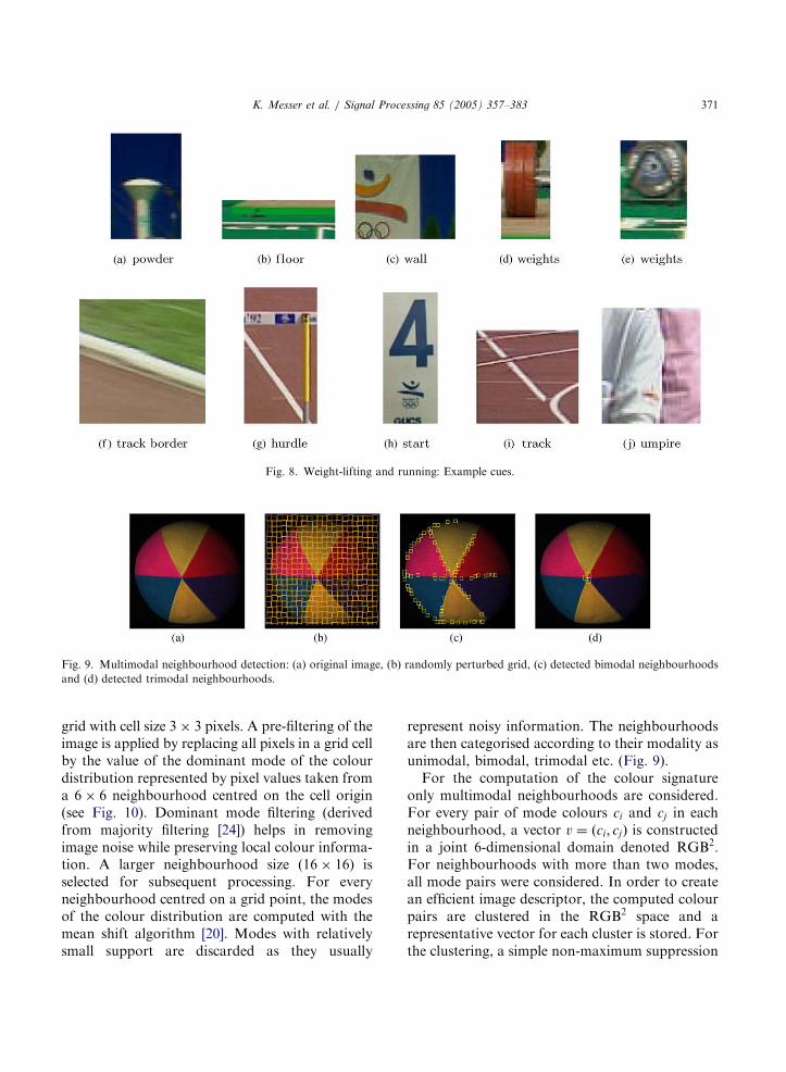
cues in the image. Some examples of cues whichare of interest in the context of the ASSAVIDproject are shown in Fig. 8. As in the previousmethod, the training process involves the extrac-tion of a set of features from a set of exampleimages showing the cue. For the cues based on thismethod, the cue training data is in the form of‘‘MNS signatures’’ taken from small regions oftraining images that contain only the cue to bedetected. In the annotation mode, the signature ismatched with measurements taken from the inputimages. From the match, information about thepresence and location of the cue in the image isobtained.In the remainder of this subsection, we discuss

the details of the feature extraction and matchingmodules.


Overview: Consider an image region consistingof a small compact set of pixels. The shape of theregion is not critical for our application. Forconvenience, we use regions defined as neighbour-hoods around a central point. Depending on thedistribution of the colour values in such a region,we characterise it as either a unimodal or amultimodal neighbourhood.A cue model is derived from measurements

computed from multimodal neighbourhoods ofone or more example images of the cue. Local

colour structure is represented by illuminationinvariant features computed from these measure-ments. The mean shift algorithm [9] is invoked toefficiently locate the peaks of the density functionin the RGB colour space.

Local processing guarantees graceful degrada-tion of performance with respect to occlusion andbackground clutter, without a need for imagesegmentation or edge detection. Multimodal (asopposed to unimodal) neighbourhoods are moreinformative in terms of colour content. The modevalues used for the computation of the invariantsare robustly filtered, stable values [19].Computing illumination invariant features from

unimodal neighbourhoods is possible under cer-tain assumptions [8]. Nevertheless, computation ofinvariants from multimodal neighbourhoods isrelatively straightforward; therefore we discardthe unimodal neighbourhoods. Little informationis lost since colours from unimodal neighbour-hoods are also usually present in the multimodalones. In particular, multimodal neighbourhoodswith more than two modes provide good char-acterisation of objects like the ball in Fig. 9(c) andcan result in efficient recognition on the basis ofonly a few features.The representation of cue appearance is flexible,

effectively using the constraints imposed by theillumination change model which in turn isdictated by the application environment. The sizeof the resulting MNS signature depends on thecomplexity of the image it describes. Typical sizesof MNS signatures are a few bytes for simplescenes, a few hundreds for more complex images.

Details of the feature extraction: The imageplane is covered by a set of overlapping smallcompact regions. Rectangular neighbourhoodswere selected since they facilitate simple and fastprocessing of the data. Image processing takesplace only for a subset of overlapping imageneighbourhoods defined by a dense rectangular

ARTICLE IN PRESS

Fig. 8. Weight-lifting and running: Example cues.

Fig. 9. Multimodal neighbourhood detection: (a) original image, (b) randomly perturbed grid, (c) detected bimodal neighbourhoods

and (d) detected trimodal neighbourhoods.


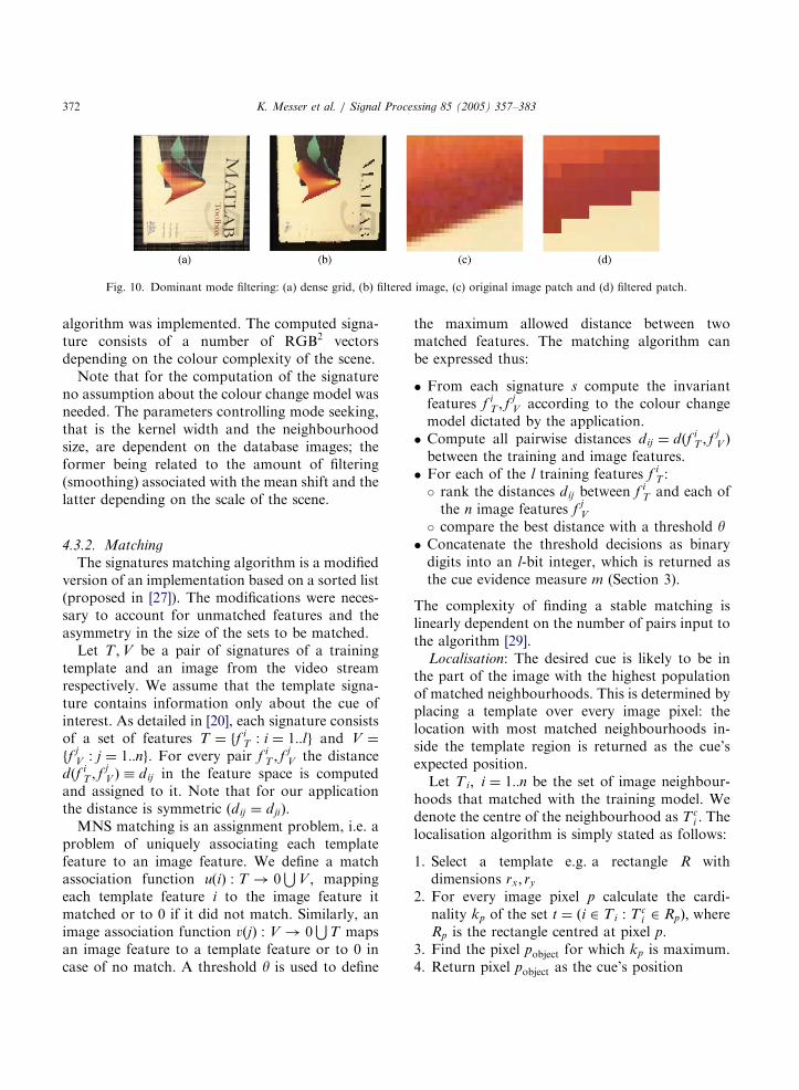
grid with cell size 3 3 pixels. A pre-filtering of theimage is applied by replacing all pixels in a grid cellby the value of the dominant mode of the colourdistribution represented by pixel values taken froma 6 6 neighbourhood centred on the cell origin(see Fig. 10). Dominant mode filtering (derivedfrom majority filtering [24]) helps in removingimage noise while preserving local colour informa-tion. A larger neighbourhood size (16 16) isselected for subsequent processing. For everyneighbourhood centred on a grid point, the modesof the colour distribution are computed with themean shift algorithm [20]. Modes with relativelysmall support are discarded as they usually

represent noisy information. The neighbourhoodsare then categorised according to their modality asunimodal, bimodal, trimodal etc. (Fig. 9).For the computation of the colour signature

only multimodal neighbourhoods are considered.For every pair of mode colours ci and cj in eachneighbourhood, a vector v ¼ ðci; cjÞ is constructedin a joint 6-dimensional domain denoted RGB2:For neighbourhoods with more than two modes,all mode pairs were considered. In order to createan efficient image descriptor, the computed colourpairs are clustered in the RGB2 space and arepresentative vector for each cluster is stored. Forthe clustering, a simple non-maximum suppression

ARTICLE IN PRESS

Fig. 10. Dominant mode filtering: (a) dense grid, (b) filtered image, (c) original image patch and (d) filtered patch.


algorithm was implemented. The computed signa-ture consists of a number of RGB2 vectorsdepending on the colour complexity of the scene.Note that for the computation of the signature

no assumption about the colour change model wasneeded. The parameters controlling mode seeking,that is the kernel width and the neighbourhoodsize, are dependent on the database images; theformer being related to the amount of filtering(smoothing) associated with the mean shift and thelatter depending on the scale of the scene.

4.3.2. Matching

The signatures matching algorithm is a modifiedversion of an implementation based on a sorted list(proposed in [27]). The modifications were neces-sary to account for unmatched features and theasymmetry in the size of the sets to be matched.Let T ;V be a pair of signatures of a training

template and an image from the video streamrespectively. We assume that the template signa-ture contains information only about the cue ofinterest. As detailed in [20], each signature consistsof a set of features T ¼ ff i

T : i ¼ 1::lg and V ¼

ffjV : j ¼ 1::ng: For every pair f i

T ; fjV the distance

dðf iT ; f

jV Þ � dij in the feature space is computed

and assigned to it. Note that for our applicationthe distance is symmetric (dij ¼ dji).MNS matching is an assignment problem, i.e. a

problem of uniquely associating each templatefeature to an image feature. We define a matchassociation function uðiÞ : T ! 0

SV ; mapping

each template feature i to the image feature itmatched or to 0 if it did not match. Similarly, animage association function vðjÞ : V ! 0

ST maps

an image feature to a template feature or to 0 incase of no match. A threshold y is used to define

the maximum allowed distance between twomatched features. The matching algorithm canbe expressed thus:

�
From each signature s compute the invariantfeatures f i
T ; fjV according to the colour change

model dictated by the application.
� Compute all pairwise distances dij ¼ dðf i
T ; fjV Þ

between the training and image features.
� For each of the l training features f i
T :� rank the distances dij between f i

T and each ofthe n image features f

jV

� compare the best distance with a threshold y
� Concatenate the threshold decisions as binarydigits into an l-bit integer, which is returned asthe cue evidence measure m (Section 3).
The complexity of finding a stable matching islinearly dependent on the number of pairs input tothe algorithm [29].

Localisation: The desired cue is likely to be inthe part of the image with the highest populationof matched neighbourhoods. This is determined byplacing a template over every image pixel: thelocation with most matched neighbourhoods in-side the template region is returned as the cue’sexpected position.Let Ti; i ¼ 1::n be the set of image neighbour-

hoods that matched with the training model. Wedenote the centre of the neighbourhood as Tc

i : Thelocalisation algorithm is simply stated as follows:

1.
Select a template e.g. a rectangle R withdimensions rx; ry
2.
For every image pixel p calculate the cardi-nality kp of the set t ¼ ði 2 Ti : Tc
i 2 RpÞ; whereRp is the rectangle centred at pixel p.

3.
Find the pixel pobject for which kp is maximum. 4. Return pixel pobject as the cue’s position

ARTICLE IN PRESS


5. Sports classifier

Let us suppose that we want to build a system torecognise a set of S different sports. The systemdesign is such that the recognition of the sport isperformed on a shot by shot basis.If we assume that for each sport we have already

ground-truthed a set of Q representative frameswhich are indicative of that sport, in total therewill be N ¼ S Q different ground-truthedimages. Fig. 11 shows some example images whichare indicative of their sport.Also, let us suppose that we have a set of C

trained cue-detectors. This set of cue detectorscould contain cue-detectors built using the neuralnet (NN), texture code (TC) and/or multi-modalneighbourhood signatures (MNS) methods. Thecues have been chosen such that they arerepresentative of objects occurring within thesports that the system is trying to categorise.Each of the N images then have this set of C cue-

detectors applied to them. So from each image avector xs

q ¼ ½x1;x2; x3; . . . ;xC � can be constructedwhere 1pqpQ and 1pspS: The elements ofthese vectors are computed by the followingformula (from (1), assuming a prior probabilityPðCÞ ¼ 1

2):

x ¼pðmjCÞ

pðmjCÞ þ pðmjCÞ: (23)

These vectors can then be used to construct alabelled dataset X of N points. Using this labelleddataset enables us to train any one of a number of

Fig. 11. Indicative images of tennis, track ev

supervised classifiers. For these experiments asimple multi-layer neural network was used. Thetraining input vectors for this classifier are thevectors of dataset X and the number of networkoutputs is equal to the number of sports. Theneural network was trained with the back-propa-gation algorithm using momentum.Once we have a trained classifier we can then use

it to analyse unknown sports video material. Thisis achieved by applying the same C cue detectorson the images taken at 1 s intervals within thesports video shot under investigation. The result-ing set of feature vectors are then applied to thetrained neural network inputs and the sum of theindividual outputs observed. The sport with thecorresponding highest mean output is the labelused to classify the shot. Fig. 12 shows theoperation of the sports classifier.

6. Experiments

The BBC provided the ASSAVID project withDV digital video tapes taken from the 1992Barcelona Olympics. Just over 5 h of this materialwas manually ground-truthed. This process in-volved first grabbing a frame every second of videofrom the DV digital tapes and storing it on disk.These frames were then manually segmented intoshots and each shot was manually assigned asports label. This data formed the basis of ourexperiments.

ents, swimming, cycling and yachting.

ARTICLE IN PRESS

Neural Net

Texture Codes

Tra

ined

neu

ral n

etw

ork

Sum

net

wor

k ou

tput

s

Sport label

Input frames of video shot

MNS

Cue Detectors Sports Classifier

Fig. 12. The shot sports classifier.

Fig. 13. Comparison of different training approaches.

Table 5

The number of different cue-detectors used from each method

Method # cue detectors


6.1. Evaluation of the cue training

Currently we have trained and tested cues foreach of the three methods described in Section 4:

Neural Net (NN) 12

Texture Codes (TC) 9
�
MNS 39
Neural Network (NN), which uses simpletexture and colour features
�
Texture Codes (TC), which uses a sophisticatedtexture representation, including some structuralinformation
�
Multimodal Neighbourhood Signatures (MNS),which uses colour combinations
We found that considerable skill was required totrain good-quality cues, as their effectiveness reliesheavily on carefully chosen examples from the test

ARTICLE IN PRESS


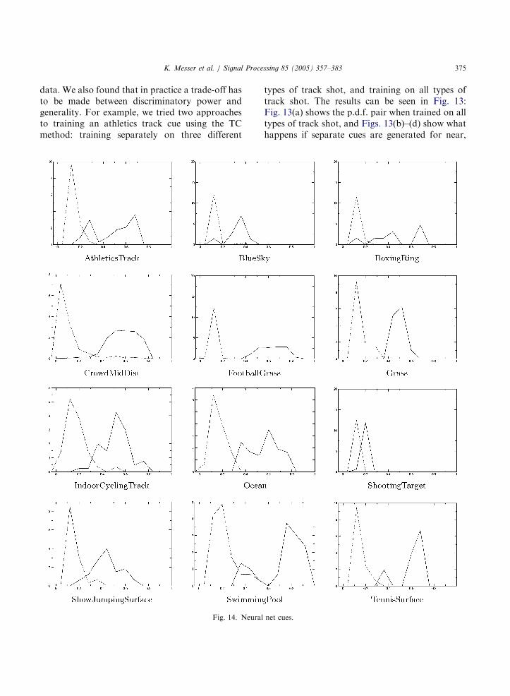
data. We also found that in practice a trade-off hasto be made between discriminatory power andgenerality. For example, we tried two approachesto training an athletics track cue using the TCmethod: training separately on three different

Fig. 14. Neural

types of track shot, and training on all types oftrack shot. The results can be seen in Fig. 13:Fig. 13(a) shows the p.d.f. pair when trained on alltypes of track shot, and Figs. 13(b)–(d) show whathappens if separate cues are generated for near,

net cues.

ARTICLE IN PRESS

Fig. 15. Texture code cues.


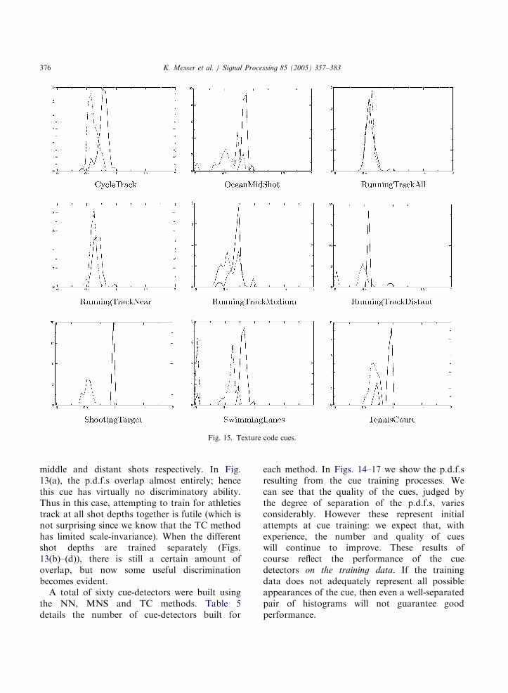
middle and distant shots respectively. In Fig.13(a), the p.d.f.s overlap almost entirely; hencethis cue has virtually no discriminatory ability.Thus in this case, attempting to train for athleticstrack at all shot depths together is futile (which isnot surprising since we know that the TC methodhas limited scale-invariance). When the differentshot depths are trained separately (Figs.13(b)–(d)), there is still a certain amount ofoverlap, but now some useful discriminationbecomes evident.A total of sixty cue-detectors were built using

the NN, MNS and TC methods. Table 5details the number of cue-detectors built for

each method. In Figs. 14–17 we show the p.d.f.sresulting from the cue training processes. Wecan see that the quality of the cues, judged bythe degree of separation of the p.d.f.s, variesconsiderably. However these represent initialattempts at cue training: we expect that, withexperience, the number and quality of cueswill continue to improve. These results ofcourse reflect the performance of the cuedetectors on the training data. If the trainingdata does not adequately represent all possibleappearances of the cue, then even a well-separatedpair of histograms will not guarantee goodperformance.

ARTICLE IN PRESS

Fig. 16. Multimodal neighbourhood signature cues (i).


6.2. Evaluation of the sports classifier

Table 6 shows which sports were represented inthe Olympics video material, and how much

material for each sport was available. Due to thelimited amount of footage available for some ofthe sports it was decided to build a classifier todistinguish between the seven sports of boxing,

ARTICLE IN PRESS

Fig. 17. Multimodal neighbourhood signature cues (ii).


cycling, hockey, swimming, tennis, track eventsand yachting.The cue-detectors described in Section 6.1 were

applied to all the images taken from the sevensports. Seven different sport classifiers were then

constructed using all the different combinations ofthese cue-detection methods (i.e. NN, MNS, TC,NN+MNS, NN+TC, MNS+TC, NN+MNS+TC). This was done using only the data taken fromthe first half of the video.

ARTICLE IN PRESS


The remaining 382 video shots were thenclassified using the different sport classifiers andcue-detection methods. Table 7 shows the numberof correctly and incorrectly classified shots. As onecan see the best individual cue-detection method is

Table 6

Manual ground-truthing of sports video

Sport Amount of material

Swimming 00:25:09:00

Track events 01:29:29:00

Boxing 00:11:27:00

Cycling 00:16:41:00

Gymnastics 00:01:22:00

Hockey 00:24:48:00

Tennis 00:09:20:00

Yachting 00:13:09:00

Judo 00:00:13:00

Medal ceremony 00:51:27:00

Others 01:06:43:00

Total 05:09:48:00

Table 7

Classification of shots and correct classification rate using

different combinations of cue-detection methods

Correct Incorrect Performance

Neural Net (NN) 247 135 0.65

Texture Codes (TC) 168 214 0.44

MNS 222 160 0.58

NN and TC 247 135 0.65

NN and MNS 266 116 0.70

TC and MNS 130 252 0.34

NN, TC and MNS 123 259 0.32

Table 8

Confusion matrix for sports classification for Neural Net. Error¼ 0:3

Boxing Cycling Hockey S

Boxing 38 0 1

Cycling 6 14 4

Hockey 36 3 81

Swimming 8 4 0 5

Tennis 4 0 0

Track events 1 3 1

Yachting 1 5 1

the neural net which achieved a correct classifica-tion performance of 0:65: The texture code methodwas the worst with a disappointing performance of0:44: The combination of the NN and MNSachieved the highest performance of 0:70:Using all the three cue-detection methods

resulted in the lowest performance of 0:32: As allthe cue-detectors were employed, the neural net-work classifier used for the sports classifica-tion had a input dimensionality of sixty. Due tothe limited amount of training material, thenumber of samples available for training somesports was too low (around one-hundred) toaccurately estimate all of the free parameters ofthe network. If we had a sufficient number oftraining samples we would expect that the resultusing all three methods would at least match thebest results obtained and would hopefully improvethe performance. Elsewhere [15] we show thatuseful improvements can be made by combiningmultiple classifiers.Tables 8, 9, 10 show the confusion matrices for

the NN, MNS and TC cue-detection methods,respectively, whilst Table 11 shows the confusionmatrix when using the NN and MNS cue-detectorstogether.

6.3. Refining the ground-truth

By analysing in more detail the shots that weremis-classified, it was found that many of the shotswere not really representative of the ground-truthsport. For example, many were of close-up shotsof the players involved or were crowd shots. Fig.18 shows sample images taken from four such mis-classified shots.

5

wimming Tennis Track events Yachting

1 0 4 0

0 0 11 0

5 0 13 1

8 1 2 4

0 2 4 0

0 6 19 0

5 0 0 35

ARTICLE IN PRESS

Table 9

Confusion matrix for sports classification for MNS. Error¼ 0:42

Boxing Cycling Hockey Swimming Tennis Track events Yachting

Boxing 21 1 0 8 0 10 4

Cycling 0 3 1 2 0 16 13

Hockey 0 3 78 5 5 41 7

Swimming 0 4 1 56 0 7 9

Tennis 0 0 1 0 4 5 0

Track events 0 1 0 3 0 25 1

Yachting 0 2 5 2 0 3 35

Table 10

Confusion matrix for sports classification for Texture Codes. Error¼ 0:66


Boxing 17 4 0 1 0 22 0

Cycling 4 9 5 1 0 13 3

Hockey 7 14 56 2 0 57 3

Swimming 9 6 8 40 0 8 6

Tennis 2 0 2 0 2 4 0


Yachting 9 2 3 2 0 11 20

Table 11

Confusion matrix for sports classification for Neural Net and MNS. Error¼ 0:30


Boxing 36 0 1 4 0 2 1

Cycling 1 19 3 3 0 6 3

Hockey 8 17 88 8 1 3 14

Swimming 1 5 0 65 0 1 5

Tennis 0 1 1 3 4 1 0


Yachting 1 8 0 4 0 0 34

Fig. 18. Images taken from some mis-classified shots. The first two are close ups of the sportsman involved. The other two are of

crowd scenes.


ARTICLE IN PRESS


For this reason the shots containing close upsand crowd scenes were taken out of the test dataset and the above set of experiments repeated.Table 12 and 13 shows the performance rates. Thistime the NN combined with MNS gave the topperformance, of 0:84; an increase of 0:14:

7. Conclusions and further work

In this paper we have described part of theASSAVID system [1], for the annotation of sportsvideo. This system is based on the concept ofcues, which allow us to extract high-level informa-tion from sets of low-level features computed onthe incoming sports video data. Three of thevisual cue methods were then outlined, togetherwith a method for using these cues to classify thetype of sport being played. The system wasshown to work well on video sequences contain-ing a selection of boxing, cycling, hockey, swim-ming, track events, tennis and yachting, with a

Table 12

Classification of shots and correct classification rate using

different combinations of cue-detection methods

Correct Incorrect Performance

Neural Net (NN) 182 54 0.77

Texture Codes (TC) 91 145 0.38

MNS 166 70 0.70

NN and TC 199 37 0.84

NN and MNS 184 52 0.78

TC and MNS 64 172 0.27

NN, TC and MNS 59 177 0.25

Table 13

Confusion matrix for sports classification for Neural Net and MNS a

Boxing Cycling Hockey S

Boxing 12 0 0

Cycling 1 15 2

Hockey 0 1 70

Swimming 1 0 0 4

Tennis 0 0 0

Track events 0 8 0

Yachting 0 8 0

correct classification performance of 84% beingachieved.The neural-net approach was a first attempt at a

sports classifier. A difficulty with this approach isobtaining sufficient (and sufficiently varied) train-ing data, and we feel that the recognition ratecould be enhanced further by using a morecomprehensive range and more representative cuesfor classifier training. Also more training data andcues would allow the system to recognise moresports. In addition we are investigating some rule-based classifier methods, including both probabil-istic and deterministic approaches.We realise that there are several types of shots

that are of little use for sports classification: close-ups, interviews (sometimes), medal ceremonies(sometimes), crowd shots. We need to be able toidentify all of these shot types, and apply sometemporal contextual reasoning to merge informa-tion from neighbouring shots.The system is still under development: within

ASSAVID we are currently developing a variety ofother cue methods, including ‘‘Speech Keywords’’,‘‘Text Keywords’’, ‘‘Non-speech Audio’’, ‘‘MotionActivity’’ and ‘‘Periodic Motion’’. We are alsodeveloping other algorithms to make other typesof decision about events happening within theaudio-visual material.

Acknowledgements

This work was performed within the frameworkof the IST-1999-13082 ASSAVID Project fundedby the European IST Programme.

fter a finer resolution of ground-truthing. Error=0:16

wimming Tennis Track events Yachting

0 0 0 1

1 0 4 0

2 0 1 0

6 0 0 3

0 2 0 0

0 0 20 0

4 0 0 34

ARTICLE IN PRESS


References

[1] Automatic segmentation and semantic annotation of

sports videos, European IST Programme: Project IST-

1999-13082 ASSAVID: http://www.cordis.lu/ist/ka4/tesss/

projects.htm.

[2] C. Bishop, Neural Networks for Pattern Recognition,

Clarendon Press, Oxford, UK, 1996.

[3] A.C. Bovik, M. Clark, W.S. Geisler, Multichannel texture

analysis using localized spatial filters, IEEE T-PAMI 12 (1)

(January 1990) 55–73.

[4] M. Cover, J.A. Thomas, Elements of Information Theory,

Willey Series in Telecommunications, Wiley, New York,

1990.

[5] I.J. Cox, S. Hingorani, S.B. Raow, A maximum likelihood

stereo algorithm, Comput. Vision Image Understand. 63

(3) (1996) 542–567.

[6] W.H. Press, et al., Numerical Recipes in C: the Art of

Scientific Computing, second ed., Cambridge University

Press, Cambridge, 1992.

[7] N. Fatemi-Ghomi, P. Palmer, M. Petrou, Performance

evaluation of texture segmentation algorithms based on

wavelets, Preceedings of the Workshop on Performance

Characteristics of Vision Algorithms, Fourth European

Conference on Computer Vision, Cambridge, April 1996,

pp. 99–119.

[8] G. Finlayson, G. Schaefer, Constrained dichromatic

colour constancy, in: D. Vernon (Ed.), Proceedings of

the Sixth European Conference on Computer Vision,

Lecture Notes in Computer Science, vol. 1842, Springer,

Berlin, Germany, June 2000, pp. 342–358.

[9] K. Fukunaga, L. Hostetler, The Estimation of the

Gradient of a Density Function, with Applications in

Pattern Recognition, in: IEEE Transactions in Informa-

tion Theory, 1975, pp. 32–40.

[10] R.M. Haralick, K. Shanmugam, I. Dinstein, Textural

features for image classification, IEEE Trans. Systems

Man Cybernetics 3 (November 1973) 610–621.

[11] D.J. Heeger, E.P. Simoncelli, J.A. Movshon, Computa-

tional models of cortical visual processing, Proc. Natl.

Acad. Sci. USA 93 (1996) 623–627.

[12] S.S. Intille, A.F. Bobick, A framework for representing

multi-agent action from visual evidence, Proceedings of the

National Conference on Artificial Intelligence (AAAI),

July 1999.

[13] A.K. Jain, F. Farrokhnia, Unsupervised texture segmenta-

tion using gabor filters, Pattern Recognition 24 (12) (1991)

1167–1186.

[14] J.G. Daugman, Uncertainty relation for resolution in

space-spatial frequency and orientation optimized by two-

dimensional visual cortical filters, J. Opt. Soc. Amer. 2

(1985) 1160–1169.

[15] J. Kittler, M. Ballette, W.J. Christmas, E. Jaser, K.

Messer, Fusion of multiple cue detectors for automatic

sports video annotation, Joint IAPR International Work-

shops on Statistical, Syntactical and Structural Pattern

Recognition (SSSPR), 2002.

[16] V. Kobla, D. DeMenthon, D. Doermann, Identifying

sporst video using replay, text and camera motion features,

SPIE Storage and retrieval for Media Database 2000,

2000, pp. 332–342.

[17] B. Levienaise-Obadia, W. Christmas, J. Kittler,

Defining quantisation strategies and a perceptual

similarity measure for texture-based annotation and

retrieval, in: IEEE (Ed.), Proceedings of the ICPR’2000,

September 2000.

[18] B. Levienaise-Obadia, J. Kittler, W. Christmas, Compara-

tive study of strategies for illumination-invariant texture

representations, in: SPIE, editor, Proceedings of the

Storage and Retrieval for Video and Image Databases

VII, January 1999.

[19] J. Matas, Colour object recognition, Ph.D. Thesis,

University Of Surrey, 1995.

[20] J. Matas, D. Koubaroulis, J. Kittler, Colour image

retrieval and object recognition using the multimodal

neighbourhood signature, in: Proceedings of the 6th

ECCV, June 2000, pp. 48–64.

[21] H. Mo, S. Satoh, M. Sakauchi, A study of image

recognition using similarity retrieval, in: First Interna-

tional Conference on Visual Information Systems (Vi-

sual’96) 1996, pp. 136–141.

[22] M.R. Naphade, T. Kristjansson, B. Frey, T.S. Huang,

Probabilistic multimedia objects (multijects): A novel

approach to video indexing and retrieval in multimedia

systems, in: Proceedings of the International Conference

on Image Processing, 1998.

[23] M.R. Naphade, T.S. Huang, Semantic video indexing

using a probabilistic framework, in: Proceedings of the

International Conference on Pattern Recognition, 2000,

pp. 83–88.

[24] K. Park, Il-Dong Yun, S. Uk Lee, Color image retrieval

using a hybrid graph representation, J. Image Vision

Comput. 17 (7) (1999) 465–474.

[25] R. Qian, N. Hearing, I. Sezan, A computational approach

to semantic event detection, in: Computer Vision and

Pattern Recognition, 1999.

[26] A.L. Ratan, W.E.L. Grimson, W.M. Wells III,

Object detection and localization by dynamic

template warping, Int. J. Comput. Vision 36 (3) (2000)

131–147.

[27] R. Sara, The class of stable matchings for computational

stereo, Technical Report CTU-CMP-1999-22, Czech

Technical University, 1999.

[28] D.D. Saur, Y.-P. Tan, S.R. Kulkarni, P.J.

Ramadge, Automated analysis and annotation of

basketball video, in: SPIE Storage and Retrieval for

Still Image and Video Databases V, vol. 3022, 1997,

pp. 176–187.

[29] R. Sedgewick, Algorithms, Addison Wesley, Reading,

MA, 1988.

[30] M.J. Swain, D.H. Ballard, Color indexing, Internat.

J. Comput. Vision 7 (1) (1991) 11–32.

[31] T. Tan, On colour texture analysis, Ph.D. Thesis,

University of Surrey, 1994.

http://www.cordis.lu/ist/ka4/tesss/projects.htm

http://www.cordis.lu/ist/ka4/tesss/projects.htm

ARTICLE IN PRESS


[32] T. Tan, J. Kittler, On colour texture representation and

classification, in: Proceedings of the second International

Conference on Image Processing, Singapore, 1992,

pp. 390–395.

[33] A. Tversky, Features of similarity, Psychol. Rev. 84 (4)

(July 1997) 327–352.

[34] N. Vasconcelos, A. Lippman, Bayesian modeling

of video editing and structure: Semantic features for

video summarization and browsing, in: Proceedings

of the International Conference on Image Processing,

1998.

[35] Virage Inc. http://www.virage.com.

http://www.virage.com

A unified approach to the generation of semantic cues for sports video annotation

Documents

Transcript of A unified approach to the generation of semantic cues for sports video annotation