A  TLD  STUDY  OF  ACUROS  XB  FOR  LUNG  SBRT    USING  A  LUNG  SUBSTITUTE  MATERIAL

   

             

 SUBMITTED    

BY    

Roger  Soh  Cai  Xiang  (U0940009B)    

SUPERVISOR:    Assoc  Prof  Lee  Cheow  Lei  James  

 CO-­‐SUPERVISOR:  

Assoc  Prof  Phan  Anh  Tuan      

     

DIVISION  OF  PHYSICS  &  APPLIED  PHYSICS  SCHOOL  OF  PHYSICAL  AND  MATHEMATICAL  SCIENCES  

   

A  final  year  project  report  presented  to    

Nanyang  Technological  University  in  partial  fulfilment  of  the    requirements  for  the  

Bachelor  of  Science  (Hons)  in  Physics  /  Applied  Physics  Nanyang  Technological  University  

   

May 2013

  2  

Abstract  

Purpose:  The  recent  development  of  a  new  photon  transport  algorithm,  Acuros  XB,  

has   shown   good   potential   to   be   an   alternative   to   the   benchmark,   Monte   Carlo  

method.  The  advantage  of  Acuros  XB  (AXB)  is  in  regions  of  significant  heterogeneity  

where   it   has   been   shown   to   be   almost   equivalent   to   Monte   Carlo   and   generally  

better  than  other  advanced  model-­‐based  algorithms.  This  project  focuses  on  the  use  

of  Thermoluminesence  Dosimeters  (TLDs)  for  the  validation  of  AXB  on  Lung  SBRT.  

A  comparison  between  AXB,  AAA  (Anisotropic  Analytical  Algorithm,  Varian  Medical  

Systems,   USA),   and   physical   TLD   measurements   in   a   lung   substitute   material  

(composition  cork)  will  be  studied.  

Methods:   A   thorough   study   was   first   done   to   prepare   and   calibrate   TLDs   for  

measurement.  Next,  a  study  of  clinical  cases  was  done  to  determine   the   treatment  

parameters  and  phantom  dimensions  for  Lung  Stereotactic  Body  Radiation  Therapy  

(SBRT)  cases.  Two  multilayered  slab  phantom,  consisting  of  combinations  of  Plastic  

WaterTM   (CIRS,   Norfolk,   VA)   and   composition   cork   was   then   built   for   TLD  

measurement.   A   corresponding   virtual   phantom   was   created   in   the   clinical  

treatment   planning   system.   Presence   of   bone   is   not   considered   in   this   study.   The  

phantom  dose  distributions  of  field  sizes  2x2,  5x5,  and  10x10  cm2  for  6  MV  photon  

beams  were   then   analysed   by   comparison   of   TLD  measurements   on   the   phantom  

against  AXB  and  AAA  calculations  on  the  virtual  phantom.  

  3  

Results:   TLDs   were   carefully   calibrated   and   the   best   linear   dose   response   range  

was   found   to   be  between  0.1-­‐1.0  Gy.  All   Lung   SBRT   treatments  were  delivered   at  

6MV  with  field  sizes  ranging  from  5x5  to  10x10  cm2.  2x2  cm2  field  size  was  included  

to   study   small   stereotactic   field   effects   in   lung  medium.  Overall   TLD   results   show  

that  AXB  was  better  than  AAA  in  the  lung  medium  and  the  lung  to  tissue  interfaces.  

Conclusion:  AXB  was  found  to  be  an  accurate  algorithm  for  lung  correction.  Based  

on   TLD   measurements,   it   is   accurate   for   AXB   dose   calculation   in   Lung   SBRT,   on  

areas    where  smaller  field  sizes  (<  10x10  cm2)  are  normally  used.  

Keywords:  Acuros,  TLD,  Lung  SBRT,  composition  cork  

  4  

Acknowlegments  When I was young, I loved superheroes from DC and Marvel comics (well, I still do). As

most superheroes have a certain involvement in the sciences, it inspired me to have this

thirst for scientific knowledge, in the hope that I might be a superhero too. One of them is

Dr. Bruce Banner, or commonly known as the Incredible Hulk. He was an extremely

intelligent radiation physicist, who was later irradiated accidentally with gamma

irradiation, transforming him into a big, green Goliath with incredible strength. Needless

to say, the Incredible Hulk uses his powers to fight crime, protect the innocent and save

the world. Being a medical physics student, I handle high doses of radiation everyday, so

as to contribute my research to help benefit the life of a cancer patient. It made me realize

that I am as close as I can get to be Bruce Banner. I am living my dream. I will like to use

this opportunity to thank the people who have helped me achieve this dream.

First of all, I will like to thank my supervisor Professor James Lee Cheow Lei, for being a

very supportive mentor to me. He is gentle, generous and patient, yet authoritative, driven

and just. He has done beyond his call as a supervisor, and even created an opportunity for

me to present my work in a Master’s Level medical physics conference as an

undergraduate. I was full of gratitude the moment I heard I won the award as one of the

best presenters. Without his guidance, this FYP will not be possible.

I will like to thank my co-supervisor Professor Phan Anh Tuan, who was also very

supportive of my work. Despite his busy schedule, he took the time to guide and show me

on how I should present my work, especially to those in the academia who are not in the

medical field. On top of that, he also showed his great support in sending me to the

medical physics conference.

I will like to thank Professor Yigal Horowitz, from Ben Gurion University, Beersheva,

Israel. He is a world-reknown expert in thermoluminesence dosimetry and author of three

volume books. Our paths crossed when I was stuck at my project and decided to e-mail

  5  

my problems to the authors of several publications I have cited. To my surprise, Professor

Horowitz replied by giving several pointers on how I should carry on with my project.

His pointers were right-on and the project was resumed. We maintained an e-mail

conversation until he saw the end of my project. I was really blessed and wish that I could

thank him personally someday.

I will like to thank Mr. Ang Khong Wei, Mr. Jerome Yap Haw Hwong and Ms. Wendy

Chow Wan Li. They are the medical physicists in National Cancer Centre Singapore

(NCCS), who have guided and mentored me in a fatherly and motherly manner. Many

times they have went beyond the call of duty by staying back after working hours, so as

to ensure our safety in handling the radiotherapy equipment.

I also like to thank my course mates, Mr. Melvin Chew Ming Long, Mr. Phua Jun Hao

and Mr. Tay Guan Heng, for all the fun times, the bad times, the happy times and the

busy times we had in NCCS. We have grown a lot by learning from one another through

this period.

I also will like to acknowledge my parents and my beloved girlfriend Ms. Chua Joo Leng,

who although have no idea what my project is about, showed continuous prayers, support

and encouragement to me. Without their emotional support, this would not have been

possible.

Lastly, I will like to thank God for being sovereign, by guiding me like “a lamp to my

feet and a light to my path” (Psa 119:105). To God be the glory.

  6  

Contents  ABSTRACT  ................................................................................................................................................  2  ACKNOWLEGMENTS  ..............................................................................................................................  4  CONTENTS  ................................................................................................................................................  6  1   INTRODUCTION  ...............................................................................................................................  8  1.1   MOTIVATION  ...................................................................................................................................................  8  1.2   OBJECTIVE  .......................................................................................................................................................  9  1.3   SCOPE  OF  THE  PROJECT  ..............................................................................................................................  10  

2   THE  PHYSICS  OF  RADIOTHERAPY  ..........................................................................................  11  2.1   INTRODUCTION  TO  RADIOTHERAPY  ........................................................................................................  11  2.2   RADIATION  DOSIMETRY  ............................................................................................................................  13  2.2.1   Absorbed  Dose  ......................................................................................................................................  13  2.2.2   Linear  Accelerators  ............................................................................................................................  14  

2.3   RADIATION  TREATMENT  SETUPS  .............................................................................................................  18  2.3.1   Source  Surface  Distance  (SSD)  Setup  .........................................................................................  18  2.3.2   Source  Axis  Distance  (SAD)  Setup  ...............................................................................................  19  

2.4   PHOTON  BEAMS  ..........................................................................................................................................  21  2.5   SUMMARY  .....................................................................................................................................................  24  

3   THERMOLUMINESENCE  DOSIMETERS  ..................................................................................  25  3.1   INTRODUCTION  TO  TLDS  ..........................................................................................................................  25  3.1.1   A  General  Model  of  Thermoluminesence  Dosimetry  ...........................................................  27  3.1.2   Characteristics  of  TLDs  ....................................................................................................................  29  3.1.3   TLD  Reader  ............................................................................................................................................  30  3.1.4   TLD  Glow  Curve  ...................................................................................................................................  32  3.1.5   TLD  setup  for  radiotherapy  ............................................................................................................  34  

3.2   TLD  MEASUREMENT  METHODS  ................................................................................................................  38  3.2.1   Element  Correction  Coefficient  .....................................................................................................  38  3.2.2   Reader  Calibration  Factor  and  Absorbed  Dose  .....................................................................  42  3.2.3   Selection  of  Calibration  and  Field  Dosimeters  .......................................................................  44  3.2.4   Linearity  of  TLD  readings  ...............................................................................................................  45  

3.3   SUMMARY  .....................................................................................................................................................  47  4   DOSE  CALCULATION  ALGORITHMS  ........................................................................................  49  4.1   ANISOTROPIC  ANALYTICAL  ALGORITHMS  (AAA)  ................................................................................  51  4.2   ACUROS  EXTERNAL  BEAM  (AXB)  ...........................................................................................................  53  4.2.1   Computed  Tomography  (CT)  number  –  mass  density  relationship  ..............................  54  

4.3   LUNG  STEREOTACTIC  BODY  RADIATION  THERAPY  (SBRT)  ..............................................................  57  4.4   SUMMARY  .....................................................................................................................................................  62  

   

  7  

5   APPLICATION  OF  TLD  TO  VALIDATE  ACUROS  XB  FOR  LUNG  SBRT  ............................  64  5.1   BACKGROUND  OF  STUDY  ...........................................................................................................................  64  5.2   METHODOLOGY  ...........................................................................................................................................  67  5.2.1   Dose  Calculation  ..................................................................................................................................  67  5.2.2   Setup  of  the  Lung  Phantom  ............................................................................................................  68  5.2.3   TLD  Calibration  and  measurement  positions  ........................................................................  70  

5.3   RESULTS  AND  DISCUSSIONS  ......................................................................................................................  72  5.3.1   Challenge  encountered  in  preliminary  TLD  study  ................................................................  72  5.3.2   Perturbation  Factors  for  TLDs  ......................................................................................................  72  5.3.3   Verification  of  AXB  and  AAA  with  TLD  measurements  ......................................................  76  5.3.4   Discussions  .............................................................................................................................................  77  

5.4   SUMMARY  .....................................................................................................................................................  82  6   CONCLUSION  ..................................................................................................................................  84  6.1   SUMMARY  .....................................................................................................................................................  84  6.2   FUTURE  WORKS  ..........................................................................................................................................  87  

7   REFERENCES  ..................................................................................................................................  88  APPENDIX  ..............................................................................................................................................  91  I.   CAVITY  THEORY  ...............................................................................................................................................  91  II.   ACUROS  XB  SOLUTION  METHODS  ...............................................................................................................  93  III.  APPENDIX  REFERENCES  ...............................................................................................................................  105  

   

  8  

 

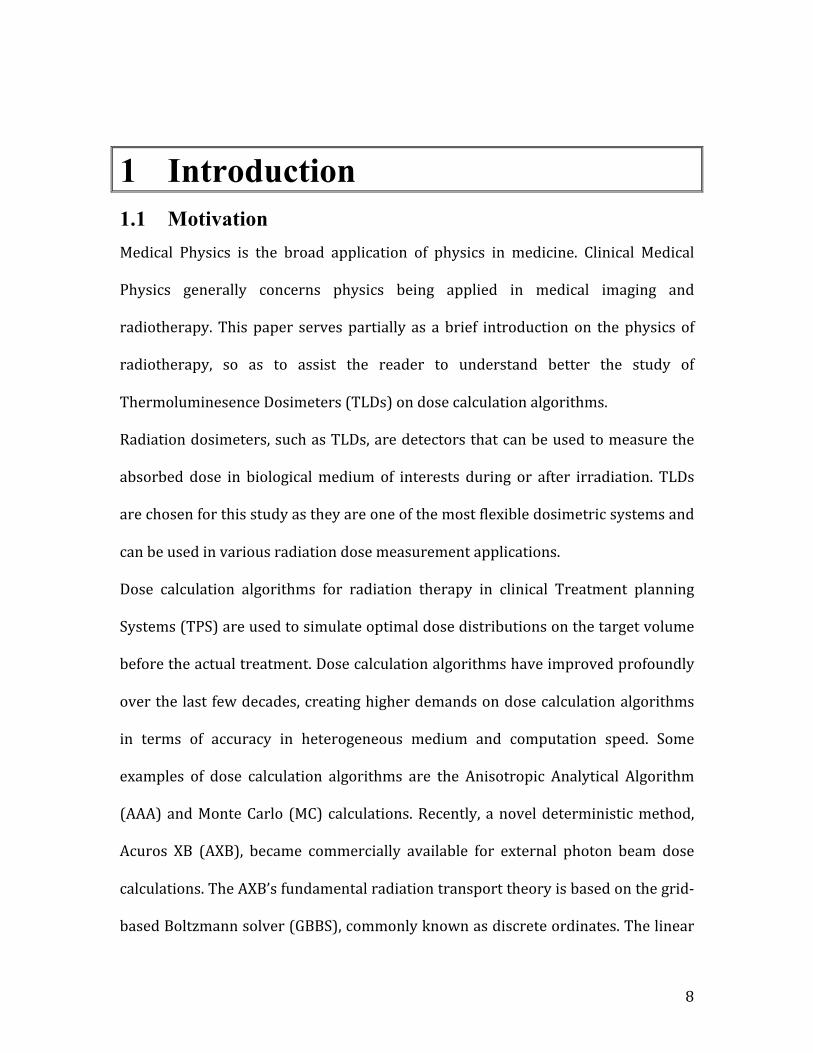
1 Introduction 1.1 Motivation Medical   Physics   is   the   broad   application   of   physics   in   medicine.   Clinical   Medical  

Physics   generally   concerns   physics   being   applied   in   medical   imaging   and  

radiotherapy.  This  paper   serves  partially   as   a  brief   introduction  on   the  physics   of  

radiotherapy,   so   as   to   assist   the   reader   to   understand   better   the   study   of  

Thermoluminesence  Dosimeters  (TLDs)  on  dose  calculation  algorithms.  

Radiation  dosimeters,  such  as  TLDs,  are  detectors  that  can  be  used  to  measure  the  

absorbed   dose   in   biological  medium   of   interests   during   or   after   irradiation.   TLDs  

are  chosen  for  this  study  as  they  are  one  of  the  most  flexible  dosimetric  systems  and  

can  be  used  in  various  radiation  dose  measurement  applications.  

Dose   calculation   algorithms   for   radiation   therapy   in   clinical   Treatment   planning  

Systems  (TPS)  are  used  to  simulate  optimal  dose  distributions  on  the  target  volume  

before  the  actual  treatment.  Dose  calculation  algorithms  have  improved  profoundly  

over  the  last  few  decades,  creating  higher  demands  on  dose  calculation  algorithms  

in   terms   of   accuracy   in   heterogeneous   medium   and   computation   speed.   Some  

examples   of   dose   calculation   algorithms   are   the   Anisotropic   Analytical   Algorithm  

(AAA)  and  Monte  Carlo   (MC)  calculations.  Recently,   a  novel  deterministic  method,  

Acuros   XB   (AXB),   became   commercially   available   for   external   photon   beam   dose  

calculations.  The  AXB’s  fundamental  radiation  transport  theory  is  based  on  the  grid-­‐

based  Boltzmann  solver  (GBBS),  commonly  known  as  discrete  ordinates.  The  linear  

  9  

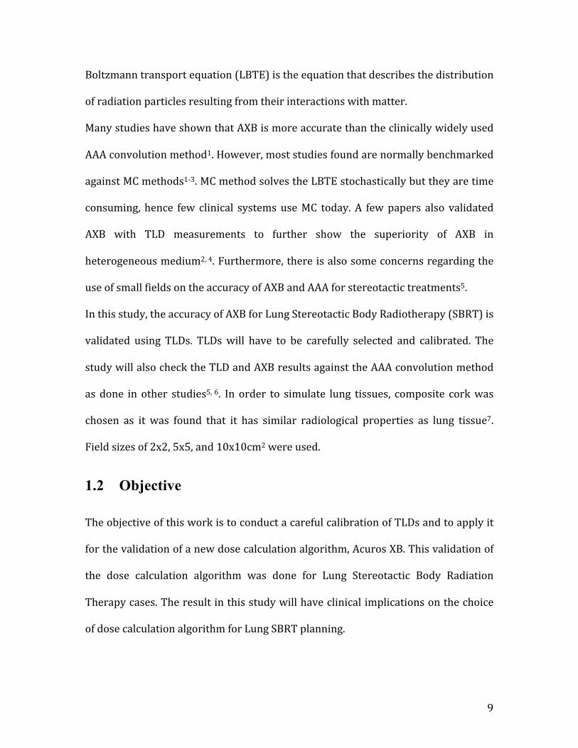
Boltzmann  transport  equation  (LBTE)  is  the  equation  that  describes  the  distribution  

of  radiation  particles  resulting  from  their  interactions  with  matter.  

Many  studies  have  shown  that  AXB  is  more  accurate  than  the  clinically  widely  used  

AAA  convolution  method1.  However,  most  studies  found  are  normally  benchmarked  

against  MC  methods1-­‐3.  MC  method  solves  the  LBTE  stochastically  but  they  are  time  

consuming,   hence   few   clinical   systems  use  MC   today.   A   few  papers   also   validated  

AXB   with   TLD   measurements   to   further   show   the   superiority   of   AXB   in  

heterogeneous  medium2,  4.  Furthermore,  there  is  also  some  concerns  regarding  the  

use  of  small  fields  on  the  accuracy  of  AXB  and  AAA  for  stereotactic  treatments5.  

In  this  study,  the  accuracy  of  AXB  for  Lung  Stereotactic  Body  Radiotherapy  (SBRT)  is  

validated   using   TLDs.   TLDs  will   have   to   be   carefully   selected   and   calibrated.   The  

study  will  also  check  the  TLD  and  AXB  results  against  the  AAA  convolution  method  

as  done   in   other   studies5,  6.   In   order   to   simulate   lung   tissues,   composite   cork  was  

chosen   as   it   was   found   that   it   has   similar   radiological   properties   as   lung   tissue7.  

Field  sizes  of  2x2,  5x5,  and  10x10cm2  were  used.  

1.2 Objective  The  objective  of  this  work  is  to  conduct  a  careful  calibration  of  TLDs  and  to  apply  it  

for  the  validation  of  a  new  dose  calculation  algorithm,  Acuros  XB.  This  validation  of  

the   dose   calculation   algorithm   was   done   for   Lung   Stereotactic   Body   Radiation  

Therapy  cases.  The  result  in  this  study  will  have  clinical  implications  on  the  choice  

of  dose  calculation  algorithm  for  Lung  SBRT  planning.    

   

  10  

1.3 Scope of the project  The  physics  of  radiotherapy  will  be  briefly  covered  in  Chapter  2  of  this  paper.  This  

will  include  radiation  dosimetry  such  as  the  concept  of  absorbed  dose,  the  usage  of  

linear  accelerators  and  the  characteristics  of  photon  beams.  

 

An   introduction   of   Thermoluminesence   Dosimetry   will   be   covered   in   Chapter   3.  

The   characteristics   of   TLDs,   TLD   reading   equipment   and   TLD   measurement  

methods  will  be  covered.  A  short  study  on  the  calibration  of   the  TLDs  will  also  be  

presented.  

 

Dose  calculation  algorithms  such  as  AAA  and  AXB  will  be  covered  in  Chapter  4.  The  

focus   in   this  chapter   is  on   the  clinical  use  and   implications  of   the  dose  calculation  

algorithm.  Note  that  the  mechanics  of  the  dose  calculation  algorithms  is  not  within  

the   scope   of   this   paper,   however,   details   of   AXB   is   covered   in  Appendix   II.   The  

creation   of   the   Lung   SBRT   phantom,   including   the   virtual   phantom,   will   also   be  

covered  in  this  chapter.  

 

Lastly,  Chapter  5  will  cover  the  validation  of  AXB  and  AAA  using  TLDs.  Through  this  

validation,  the  implications  of  using  different  algorithms  in  a  Lung  SBRT  treatment  

will   be   evaluated.   Perturbation   factors   for   of   TLDs   for   lung   medium  will   also   be  

explained  and  applied  to  the  measurement.  

   

  11  

2 The Physics of Radiotherapy 2.1 Introduction to Radiotherapy  Physics  is  extremely  essential  in  cancer  therapy.  For  example,  radiotherapy  was  first  

used  to  treat  breast  cancer  patients  shortly  after  the  discovery  of  X-­‐rays  by  German  

physicist,   Wilhelm   Röntgen.   Currently,   radiotherapy   is   a   common   form   of   cancer  

treatment  for  most  cancer  cases.  Basically,  it  involves  having  a  high-­‐energy  photon  

beam  directed  towards  a  cancer  patient’s  tumor.  

 

Cells   are   damaged  when   irradiated   as   radiation   forms   extremely   reactive   radicals  

within  the  cell.  These  radicals  cause  the  DNA  bonds  to  be  chemically  broken  down,  

resulting  in  the  cell’s  inability  to  reproduce.  With  increased  dosage,  the  probability  

of  sterilizing  cells  increases.  However,  both  the  malignant  cells  and  the  healthy  cells  

will  experience  the  same  damage  when  irradiated.  Thus,  there  is  a  need  to  spare  the  

healthy  cells  during  irradiation.  

 

Thankfully,  there  is  a  minor  contrast  in  the  radiation  response  of  malignant  cells  and  

healthy  cells.  This  difference  in  radiation  response  prevents  the  healthy  cells  within  

the  target  volume,  and  the  nearby  tissues,  from  being  destroyed.  This  phenomenon  

is  probably  due  to  several  reasons  such  as  the  cell’s  radiosensitivity  and  differences  

in   the   genetic   mechanism   that   is   affected   by   radiation8.   In   order   to   magnify   this  

radiation   response,   radiation   is  delivered   in   small  doses  per   treatment,   termed  as  

  12  

fractions.  Such  an  approach  generally  allows  therapeutic  advantage  as  compared  to  

a  single  radiation  treatment.  

In  a  normal  radiotherapy  treatment,  usually  30  fractions  of  around  2  Grays  (Gy)i  are  

used.   A   usual   treatment   last   approximately   5   to   8   weeks   where   each   fraction   is  

treated   once   a   day.   Frequency   of   the   treatment   may   be   increased  

(hyperfractionated),   by   delivering   the   fractions   twice   daily,   or   decreased   by  

delivering  higher  doses  in  lesser  fractions  (hypofractionated).  

The   second   approach   for   reducing   radiation   damage   is   to   decrease   the   dose  

delivered   to   healthy   tissues.   This   can   be   done   by   proper   radiation   treatment  

planning  and  shaping  of  the  radiation  beam  as  discussed  in  2.2.2.  

                                                                                                               i Radiation absorbed dose is defined as the energy imparted per unit mass of the irradiated

  13  

2.2 Radiation Dosimetry  Radiation dosimetry generally involves finding out how much energy is deposited in a

given medium due to ionizing radiation. In this section we will define some dosimetric

quantities below.

2.2.1 Absorbed Dose

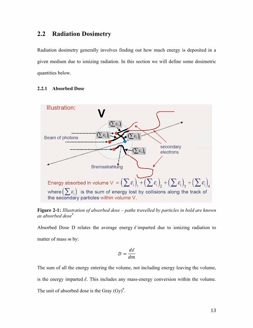
Figure 2-1: Illustration of absorbed dose – paths travelled by particles in bold are known as absorbed dose9  Absorbed Dose D relates the average energy 𝜀  imparted due to ionizing radiation to

matter of mass m by:

𝐷 =𝑑𝜀𝑑𝑚

The sum of all the energy entering the volume, not including energy leaving the volume,

is the energy imparted 𝜀. This includes any mass-energy conversion within the volume.

The unit of absorbed dose is the Gray (Gy)9.

DOSIMETRIC QUANTITIESAbsorbed dose

  14  

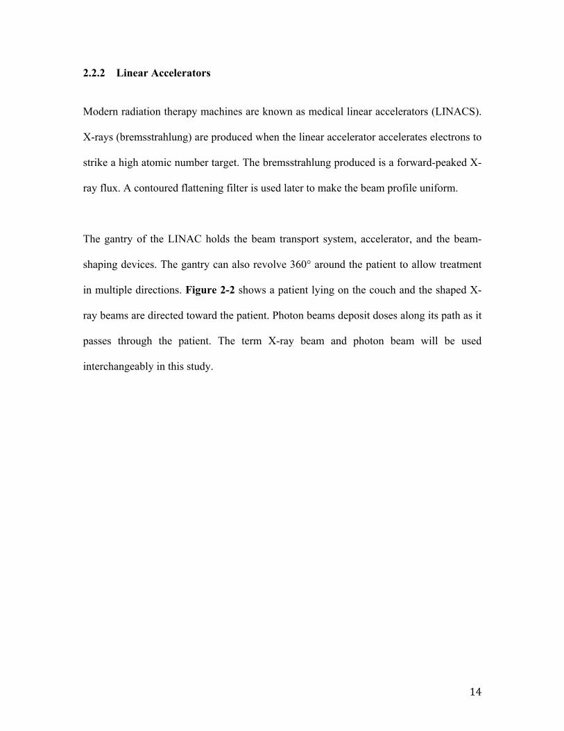
2.2.2 Linear Accelerators

 Modern radiation therapy machines are known as medical linear accelerators (LINACS).

X-rays (bremsstrahlung) are produced when the linear accelerator accelerates electrons to

strike a high atomic number target. The bremsstrahlung produced is a forward-peaked X-

ray flux. A contoured flattening filter is used later to make the beam profile uniform.

The gantry of the LINAC holds the beam transport system, accelerator, and the beam-

shaping devices. The gantry can also revolve 360° around the patient to allow treatment

in multiple directions. Figure 2-2 shows a patient lying on the couch and the shaped X-

ray beams are directed toward the patient. Photon beams deposit doses along its path as it

passes through the patient. The term X-ray beam and photon beam will be used

interchangeably in this study.

  15  

Figure 2-2: Illustration of the Linear Accelerator (LINAC) 8, 10

In radiation physics, there is some terminology that is used often to describe several

calibration points. In this section, such terminology will be introduced.

The primary transmission ionizing chamber in the LINAC measures in terms of monitor

units (MUs).

Applications of Thermoluminescent Dosimeters in Medicine 433

Fig. 11. Illustration of dose to normal tissues outside of the actual treatment field during the radiotherapy deliveryto a head and neck cancer patient.

problems taking into account individual variations in body shape and size. It is importantto caution that positional uncertainties in the placement of the TLDs in regions of highdose gradient may lead to inaccurate interpretation of the results.

Quality assurance for individual patients. With the advent of very complex radiotherapytechniques such as Intensity Modulated Radiation Therapy (IMRT) it has become com-mon practice to verify the treatment delivery sequence for individual patients. In IMRT theradiation treatment is delivered using multiple radiation fields each segmented into manysub-fields. As such, a total target dose may be delivered using many small abutting fieldsegments with an overall incident dose that is an order of magnitude larger than the result-ing dose. The ‘mix and match’ is complex and the fluency distribution in individual fieldscannot intuitively verified. Therefore, it is common practice to accurately verify the dosein IMRT treatment using a dosimeter that can determine the dose at one or more points(typically including the prescription point). Ionization chambers are usually used in thesemeasurements but they are bulky and fragile. TLDs can be appropriate especially for smallvolumes with homogeneous dose distributions. In these circumstances which may arise insimultaneous in-field boost scenarios (Fogliata et al., 2003) small detectors such as TLDsmay be the detector of choice. The measurements can be performed on a flat solid waterphantom or on an anthropomorphic phantom as previously described.In addition to point dose measurements, the dose distribution in one or more planes

through the target region can be of interest. An alternative to film may be sheets of TLdosimeters as shown in Figure 12 (courtesy of Keithley Instruments) (Iwata et al., 1995).Although not yet in common practice, medical physicists are searching for a replacementfor radiographic film in these applications since film processing has become less widelyavailable due to the increasing use of digital radiography.

  16  

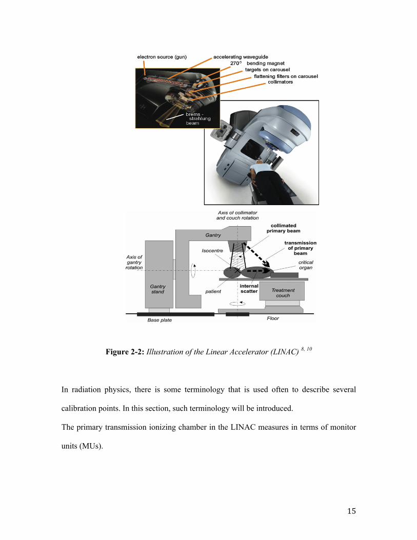
Typically, in a standard calibration setup,

• 1 MU corresponds to dose of 1cGy

• delivered in a water phantom at the depth dose maximum (zmax , Figure 2-3)

• on a central beam axis

• for 10x10cm2 field

• at a source-surface distance (SSD) or source-axis distance (SAD)

Figure 2-3: A typical depth dose profile. Regions between depth = 0cm to zmax is known as the build-up region. The depth dose maximum is at zmax. This is the point in the depth dose profile where beams are calibrated    

PENETRATION OF PHOTON BEAMS INTO PATIENTBuildup region

Build  up  Region  

  17  

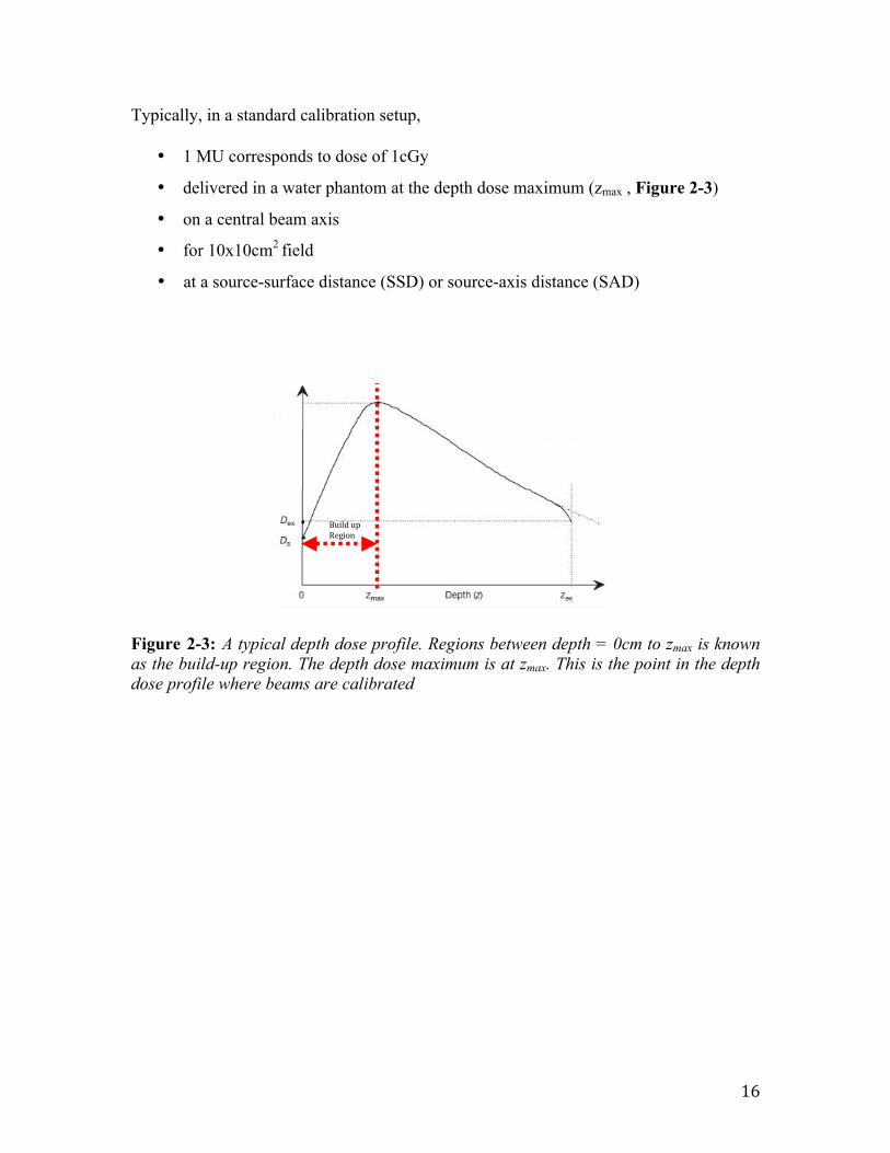
Figure 2-4: Diagram showing the setup of the central beam axis and the definition of SSD (left)9, and the setup of a 10x10cm2 field on a Plastic WaterTM phantom (right). A phantom is a mass of material that used to simulate radiological effects on biological tissue. Water and Plastic WaterTM is often used to in medical physics to simulate human adipose tissue.    

Figure 2-5: Illustration on a) how a photon beam is shaped b) lateral dose profile of the shaped beam at various depths9, this will be discussed further in section 2.4.

GAMMA RAY BEAMS AND GAMMA RAY UNITSDose delivery with teletherapy machines

(80cm for Co60 machines)

SSD = Source-Surface Distance

SDD = Source-Diaphragm Distance

 

Beam collimationLINACS

(Assuming a flat surface on water)

b)  a)  

  18  

2.3 Radiation treatment setups

2.3.1 Source Surface Distance (SSD) Setup

 

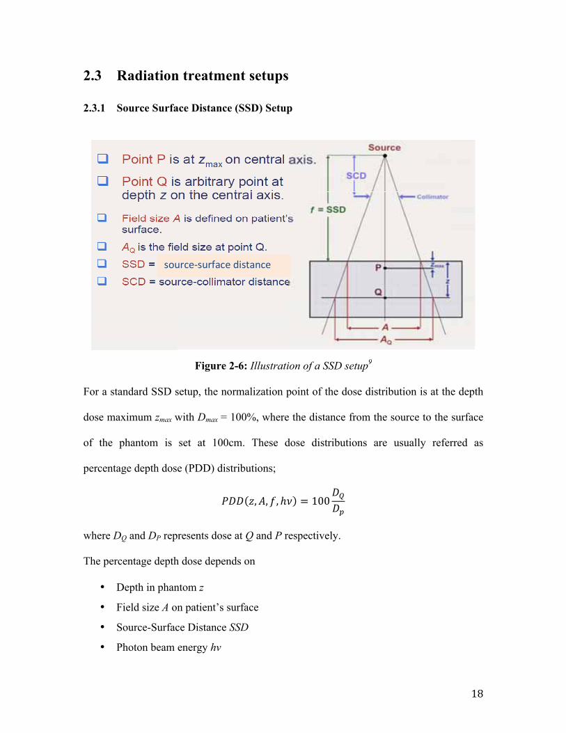
Figure 2-6: Illustration of a SSD setup9  For a standard SSD setup, the normalization point of the dose distribution is at the depth

dose maximum zmax with Dmax = 100%, where the distance from the source to the surface

of the phantom is set at 100cm. These dose distributions are usually referred as

percentage depth dose (PDD) distributions;

𝑃𝐷𝐷 𝑧,𝐴, 𝑓, ℎ𝜈 = 100𝐷!𝐷!

where DQ and DP represents dose at Q and P respectively.

The percentage depth dose depends on

• Depth in phantom z

• Field size A on patient’s surface

• Source-Surface Distance SSD

• Photon beam energy hν

RADIATION TREATMENT PARAMETERS

source-­‐surface  distance  

  19  

2.3.2 Source Axis Distance (SAD) Setup

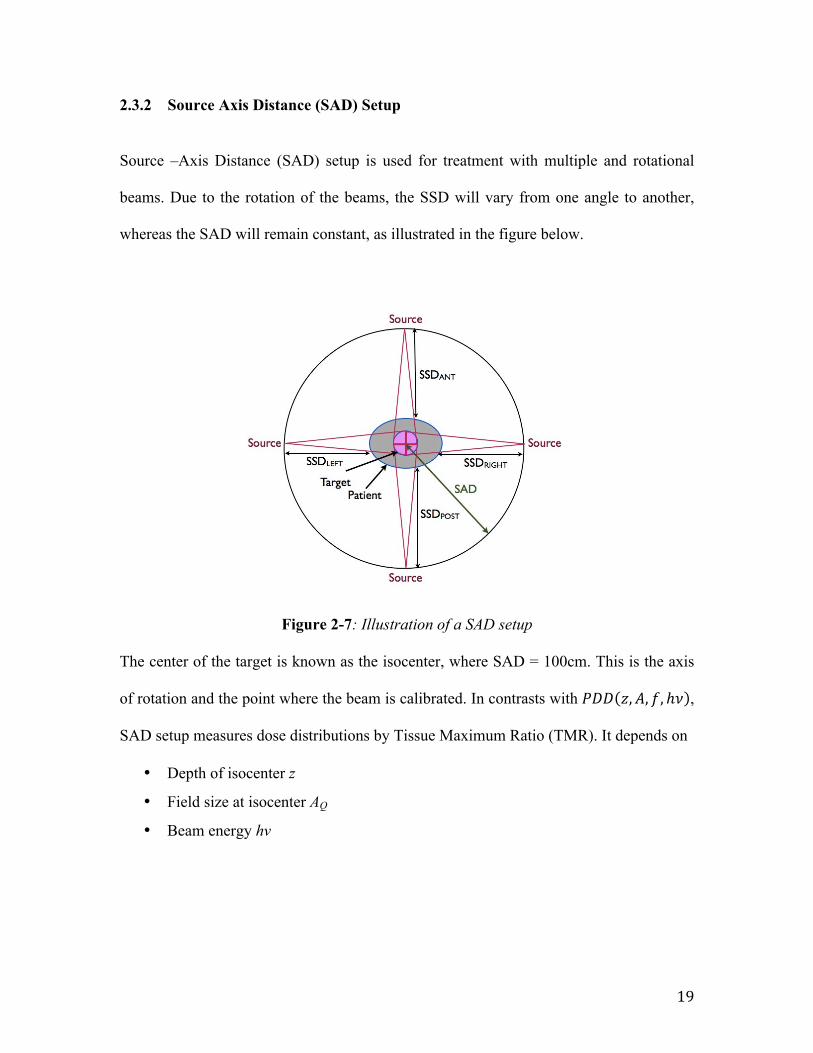
 Source –Axis Distance (SAD) setup is used for treatment with multiple and rotational

beams. Due to the rotation of the beams, the SSD will vary from one angle to another,

whereas the SAD will remain constant, as illustrated in the figure below.

Figure 2-7: Illustration of a SAD setup  The center of the target is known as the isocenter, where SAD = 100cm. This is the axis

of rotation and the point where the beam is calibrated. In contrasts with 𝑃𝐷𝐷 𝑧,𝐴, 𝑓, ℎ𝜈 ,

SAD setup measures dose distributions by Tissue Maximum Ratio (TMR). It depends on

• Depth of isocenter z

• Field size at isocenter AQ

• Beam energy hν

  20  

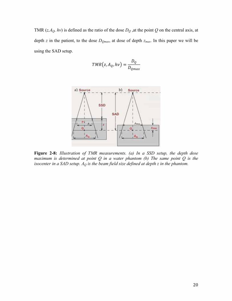
TMR (z,AQ, hν) is defined as the ratio of the dose DQ ,at the point Q on the central axis, at

depth z in the patient, to the dose DQmax, at dose of depth zmax. In this paper we will be

using the SAD setup.

𝑇𝑀𝑅 𝑧,𝐴! , ℎ𝜈 =𝐷!

𝐷!"#$

Figure 2-8: Illustration of TMR measurements. (a) In a SSD setup, the depth dose maximum is determined at point Q in a water phantom (b) The same point Q is the isocenter in a SAD setup. AQ is the beam field size defined at depth z in the phantom.

CENTRAL AXIS DEPTH DOSES IN WATER: SAD SETUPTissue-phantom ratio TPR and Tissue-maximum ratio TMR

a)   b)  

  21  

2.4 Photon Beams Factors that affect a single photon beam are:

1. beam energy (photon energy)

2. beam direction (beam angle with respect to a point within the patient)

3. beam intensityii

4. shape of the fieldiii

5. beam profileiv

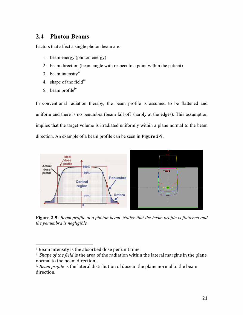
In conventional radiation therapy, the beam profile is assumed to be flattened and

uniform and there is no penumbra (beam fall off sharply at the edges). This assumption

implies that the target volume is irradiated uniformly within a plane normal to the beam

direction. An example of a beam profile can be seen in Figure 2-9.  

Figure 2-9: Beam profile of a photon beam. Notice that the beam profile is flattened and the penumbra is negligible  

                                                                                                               ii  Beam  intensity  is  the  absorbed  dose  per  unit  time. iii  Shape  of  the  field is  the  area  of  the  radiation  within  the  lateral  margins  in  the  plane  normal  to  the  beam  direction. iv  Beam profile is  the  lateral  distribution  of  dose  in  the  plane  normal  to  the  beam  direction.

OFF-AXIS RATIOS AND BEAM PROFILES

  22  

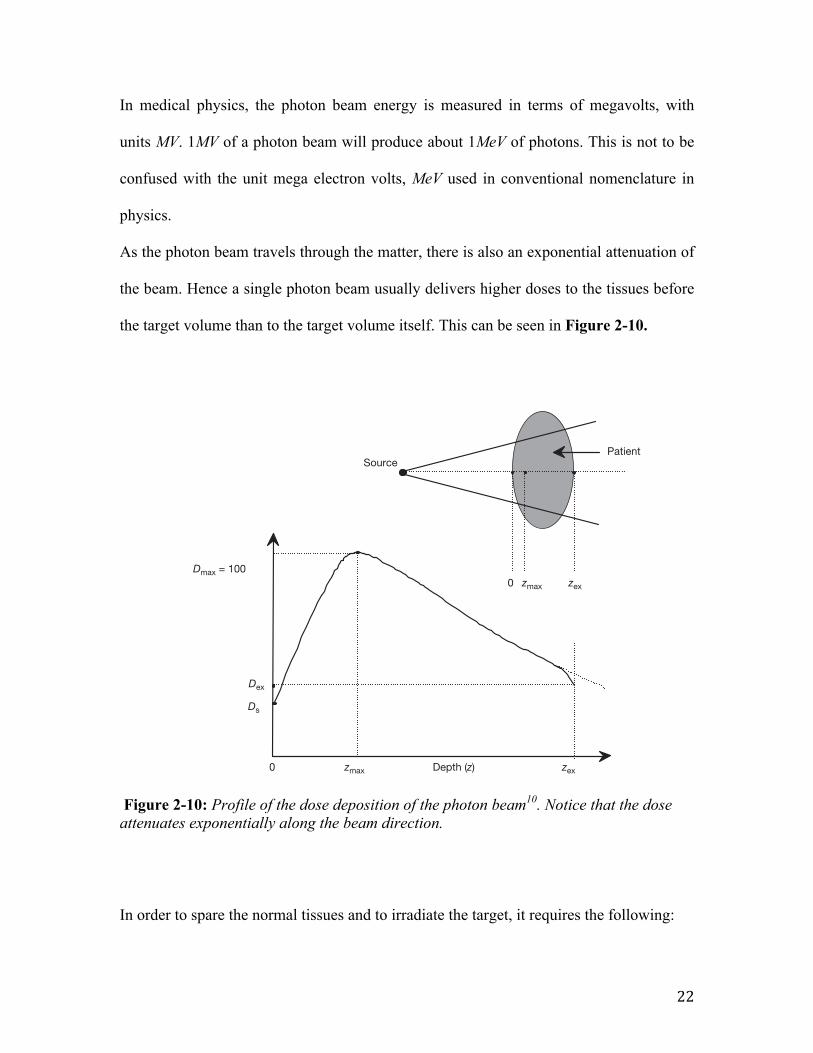
In medical physics, the photon beam energy is measured in terms of megavolts, with

units MV. 1MV of a photon beam will produce about 1MeV of photons. This is not to be

confused with the unit mega electron volts, MeV used in conventional nomenclature in

physics.

As the photon beam travels through the matter, there is also an exponential attenuation of

the beam. Hence a single photon beam usually delivers higher doses to the tissues before

the target volume than to the target volume itself. This can be seen in Figure 2-10.

Figure 2-10: Profile of the dose deposition of the photon beam10. Notice that the dose attenuates exponentially along the beam direction.

In order to spare the normal tissues and to irradiate the target, it requires the following:

CHAPTER 6

170

The functions are usually measured with suitable radiation detectors in tissue equivalent phantoms, and the dose or dose rate at the reference point is determined for, or in, water phantoms for a specific set of reference conditions, such as depth, field size and source to surface distance (SSD), as discussed in detail in Section 9.1.

A typical dose distribution on the central axis of a megavoltage photon beam striking a patient is shown in Fig. 6.3. Several important points and regions may be identified. The beam enters the patient on the surface, where it delivers a certain surface dose Ds. Beneath the surface the dose first rises rapidly, reaches a maximum value at depth zmax and then decreases almost exponentially until it reaches a value Dex at the patient’s exit point. The techniques for relative dose measurements are discussed in detail in Section 6.13.

0

Ds

Source

0

Patient

Dmax = 100zmax zex

Dex

zmax Depth (z) zex

FIG. 6.3. Dose deposition from a megavoltage photon beam in a patient. Ds is the surface dose at the beam entrance side, Dex is the surface dose at the beam exit side. Dmax is the dose maximum often normalized to 100, resulting in a depth dose curve referred to as the percentage depth dose (PDD) distribution. The region between z = 0 and z = zmax is referred to as the dose buildup region.

  23  

• Medical images to indicate the margins of the tumor and affected critical organs

• Patient positioning and immobilization

• Treatment planning – determination of the procedures in delivering the dose to the

tumor and shielding critical organs and healthy tissues. A computer simulation of

the treatment will be done to simulate the treatment procedures and fractionation

schemes

Treatment planning and evaluation is done virtually as it is able to simulate:

• Output of the LINAC

• interaction of radiation with matter - absorbed dose

• patient geometry

• the required number of beams from desired direction(s)

• dose distribution in the patient.

In summary, the planning process is the task of determining the method to treat a patient

with a virtual therapy machine, with the assumption that it is a good simulation of the

actual treatment. The treatment planning process will be discussed further in later

chapters.

   

  24  

2.5 Summary  The end goal in radiation physics is to create an optimum situation where the radiation

dose is targeted at a target volume, with the appropriate amount of dose, and yet

minimizing dose to critical organs and healthy tissues.

The concept of absorbed dose is introduced as the relationship between the average

energy 𝜀  imparted by ionizing radiation to matter of mass m.

Modern radiotherapy machines are known as Linear Accelerators. LINAC creates the

high energy X-ray beam for radiotherapy. Several parameters of the photon beams are

introduced such as depth dose maximum and monitor units.

Lastly, there are two different radiation treatment setups, source-surface distance (SSD)

and source-axis distance (SAD). In this paper, we will use the SAD setup.

  25  

3 Thermoluminesence Dosimeters 3.1 Introduction to TLDs Radiation dosimeters are used to measure absorbed dose in a medium of interest during

or after irradiation. Absorbed dose is determined by the radiation dosimeter response. The

average absorbed dose in the medium can be related to the absorbed dose in the

dosimeter sensitive volume, by using several theoretical considerations, such as cavity

theory (Appendix I). Ionization chambers, films, MOSFET detectors, semiconductor

diodes, and thermoluminescent dosimeters (TLDs) are some examples of radiation

dosimeters.

Thermoluminescence dosimetry is one of the most flexible dosimetric systems and can be

used in various radiation dose measurement applications. It was reported that the first

medical use of TLD was in 1953 by Daniels et al.11

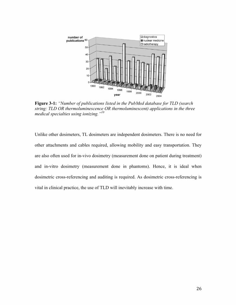
Mobit et al10 did a study and indicated that “radiotherapy is by far the most important

area in medicine where TLD is used”. It was shown in the study that “about 10 times

more papers are published annually concerning the use of TLD in radiotherapy

applications in comparison to using TLD for diagnostic procedures”   10 (Figure 3-1).

These include in-vivo dosimetry, which involve dose measurements done on patients and

in phantoms.

  26  

Figure 3-1: “Number of publications listed in the PubMed database for TLD (search string: TLD OR thermoluminescence OR thermoluminescent) applications in the three medical specialties using ionizing.”10

Unlike other dosimeters, TL dosimeters are independent dosimeters. There is no need for

other attachments and cables required, allowing mobility and easy transportation. They

are also often used for in-vivo dosimetry (measurement done on patient during treatment)

and in-vitro dosimetry (measurement done in phantoms). Hence, it is ideal when

dosimetric cross-referencing and auditing is required. As dosimetric cross-referencing is

vital in clinical practice, the use of TLD will inevitably increase with time.

Applications of Thermoluminescent Dosimeters in Medicine 413

1. Introduction

Thermoluminescence dosimetry (TLD) has a long history in medicine. Daniels (Danielset al., 1953), one of the pioneers of TLD, reported the first ‘medical’ application of TLDover half a century ago: “The crystals were swallowed by the patient (who had receivedan injection containing radioactive isotopes), recovered one or two days later, and the ac-cumulated dosage in roentgens was measured by matching thermoluminescence intensitywith that produced in crystals by a known roentgen dosage”.However, despite its many advantages, the use of TLD in medical applications has stag-

nated over the last few decades. Figure 1 shows the number of publications on TLD in threemedical subspecialties. The figure shows the publications listed with the keywords “TLD”,“thermoluminescent” or “thermoluminescence dosimetry” and a reference to radiotherapy,diagnostic radiology or nuclear medicine as listed in the PubMed database. The number ofpublications on the use of TLD in the medical field has stayed more or less constant overthe last 15 years (and beyond) despite increasingly complex irradiation geometries and anincreasing need for quality assurance and treatment dose verification.Figure 1 also indicates that radiotherapy is by far the most important area in medicine

where TLD is used. About 10 times more papers are published annually concerning theuse of TLD in radiotherapy applications than in diagnostic procedures. While most ofthe applications in diagnostic procedures are concerned with radiation protection in oneform or another, there are many more applications in radiotherapy. These include dosemeasurements in phantoms and directly on patients (“in vivo” dosimetry).The structure of the present chapter reflects this to a certain degree: after a very con-

cise discussion of some of the theoretical features of TLD relevant to medical applications,a brief overview of TLD applications in radiation protection is presented. This is followedby sections on the three most important areas of application in radiation medicine: radio-therapy, diagnostic radiology and nuclear medicine. The section on dosimetric intercom-

Fig. 1. Number of publications listed in the PubMed database for TLD (search string: TLD OR thermolumines-cence OR thermoluminescent) applications in the three medical specialties using ionizing.

  27  

3.1.1 A General Model of Thermoluminesence Dosimetry

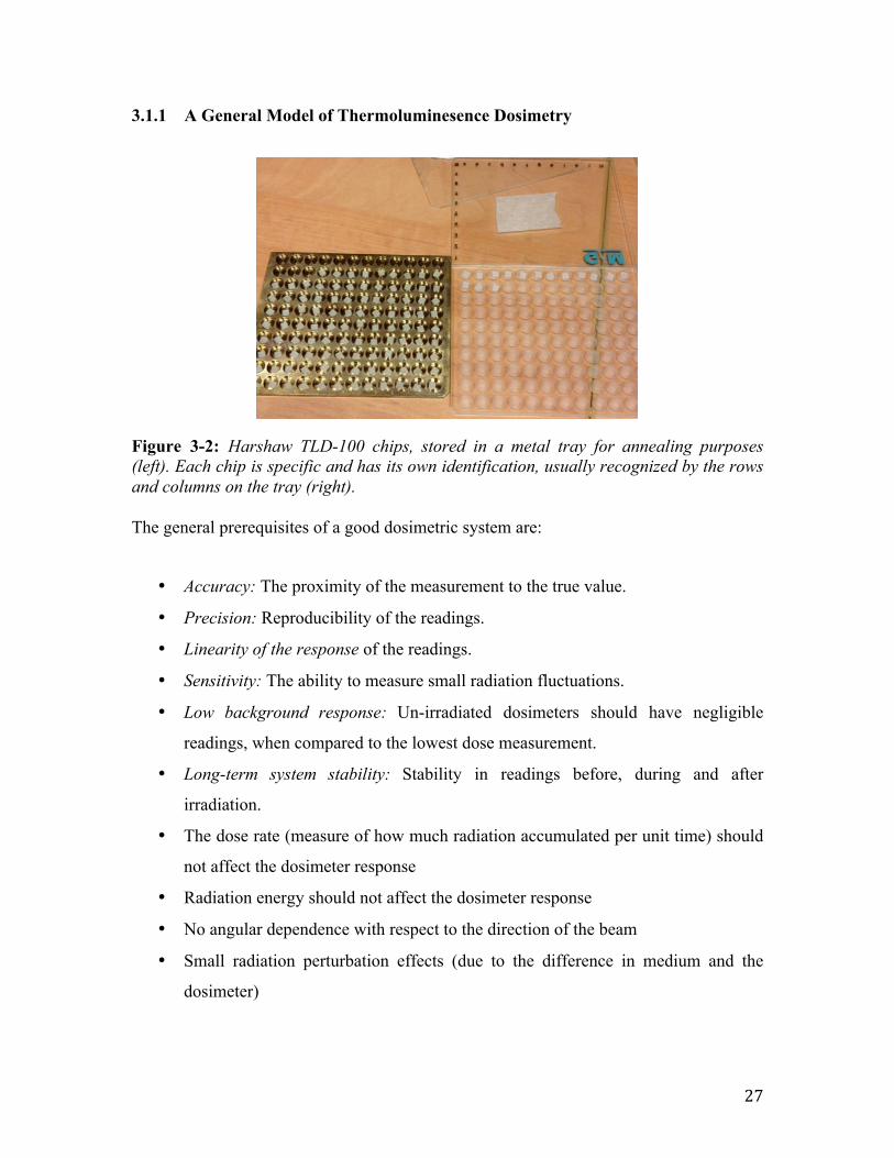
Figure 3-2: Harshaw TLD-100 chips, stored in a metal tray for annealing purposes (left). Each chip is specific and has its own identification, usually recognized by the rows and columns on the tray (right).  The general prerequisites of a good dosimetric system are:

• Accuracy: The proximity of the measurement to the true value.

• Precision: Reproducibility of the readings.

• Linearity of the response of the readings.

• Sensitivity: The ability to measure small radiation fluctuations.

• Low background response: Un-irradiated dosimeters should have negligible

readings, when compared to the lowest dose measurement.

• Long-term system stability: Stability in readings before, during and after

irradiation.

• The dose rate (measure of how much radiation accumulated per unit time) should

not affect the dosimeter response

• Radiation energy should not affect the dosimeter response

• No angular dependence with respect to the direction of the beam

• Small radiation perturbation effects (due to the difference in medium and the

dosimeter)

  28  

There are other important factors such as cost, easy usage and the ability of the dosimeter

to provide an instant reading. It is indeed difficult for dosimetric systems to meet all of

the above requirements. However, depending on the dosimetric application, optimum

measurement capability can be achieved by balancing the advantages and disadvantages

of the chosen dosimetric system.

Advantages of thermoluminescence dosimetry

• Relatively cheap and easy to use

• Able to reuse

• Versatile – Depending on the radiation therapy dose measurement

applications, TLDs are available in many forms such as rods, chips, powder,

cards and discs to suit the situation

• Small perturbation of the radiation field due to its small size. Perturbation

effects can be corrected (Chapter 5.4.1)

• High spatial resolution

• No angular dependence

• No dependence on temperature and pressure of the environment

• TLDs are stand alone detectors and require no electrical connections

Disadvantages of thermoluminesence dosimetry systems

• For accurate dosimetry, significant effort is required for calibration

• Fading of the radiation induced signal will increase with time

• Fragile, care is needed in handling TLDs

• Precision of the measurements require strict operational procedures

• TLDs must be annealed and re-calibrated

• Long annealing process (~4 hours)

• Readings will be lost after readout

  29  

3.1.2 Characteristics of TLDs

 In this paper, the TLDs used were Harshaw TLD-100 chips, which are Lithium Fluoride

crystals doped with Magnesium and Titanium ( LiF:Mg,Ti ). TLD-100 are often used

clinically for measurements of radiation dose as it has an effective atomic number of 8.2,

which is close to that of water or biological tissue10.

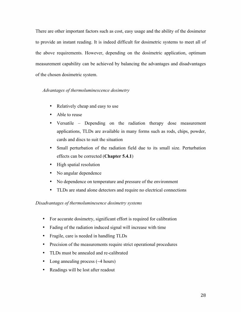
Figure 3-3: Diagram of the themoluminesence process12

Thermoluminesence (TL) crystals contain impurities (dopants) that disrupt the order of

the crystal lattice, creating trapping sites. These dopants provide additional energy levels

between the valance band and conduction band of the TL material. When irradiated, free

electrons and holes are excited may be trapped in these trapping sites. During the growth

process of the TLDs, the impurities are doped into their crystal structure with extremely

low concentration. In the case of TLD-100, the concentration of Ti is ~10ppm (parts per

million). When the TL material is heated, trapped electrons /holes will be released due to

the vibration of the atoms in the crystal lattice. The diagram of the thermoluminesence

process is shown in Figure 3-3 and Figure 3-4.

2. Theory

2.1. Thermoluminescence Dosimetry - A general model

Luminescence is a process in which, a material that is irradiated, absorbs

energy which is then emitted as a photon in the visible region of the electromagnetic

spectrum. Thermoluminescence is a form of luminescence in which heat is given to

the material which results in light emission [4].

In a crystal, electrons (e-) are found in the valence band (see figure 2.1.1a).

When the material is irradiated, e- move from the valence to the conduction band

where they move freely. Therefore, a hole (h) remains in the valence band (absence of

electron) which can also move inside the crystal. Due to impurities and doping of the

crystal, e- and h traps are created in the band gap between the valence and the

conduction band. Thus e- and h are trapped at defects (figure 2.1.1b). If these traps are

deep, the electrons and holes will not have enough energy to escape. By heating the

crystal their energy is increased, they leave the traps and recombine at luminescence

centers. As a result light is then emitted (figure 2.1.1c) [4-5].

(a) (b) (c)

Figure 2.1.1: The mechanism of TL dosimetry [5].

A TLD can be considered as an integrating detector in which the number of e-

and h, which are trapped, is the number of the e-/h pairs which are produced during

the exposure. Preferably, every trapped e-/h emits one photon. Consequently, the

number of emitted photons is equal to the number of charge pairs, which are also

proportional to the dose which is absorbed by the crystal [6].

3

  30  

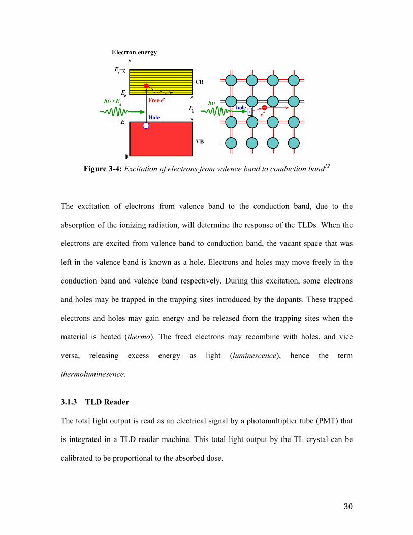
Figure 3-4: Excitation of electrons from valence band to conduction band12

The excitation of electrons from valence band to the conduction band, due to the

absorption of the ionizing radiation, will determine the response of the TLDs. When the

electrons are excited from valence band to conduction band, the vacant space that was

left in the valence band is known as a hole. Electrons and holes may move freely in the

conduction band and valence band respectively. During this excitation, some electrons

and holes may be trapped in the trapping sites introduced by the dopants. These trapped

electrons and holes may gain energy and be released from the trapping sites when the

material is heated (thermo). The freed electrons may recombine with holes, and vice

versa, releasing excess energy as light (luminescence), hence the term

thermoluminesence.

3.1.3 TLD Reader

The total light output is read as an electrical signal by a photomultiplier tube (PMT) that

is integrated in a TLD reader machine. This total light output by the TL crystal can be

calibrated to be proportional to the absorbed dose.

Electrons and holes in silicon crystalElectrons and holes in silicon crystal

• WhenȱaȱphotonȱbreaksȱaȱSiȬSiȱ bond,ȱaȱfreeȱelectronȱandȱaȱ

holeȱinȱtheȱSiȬSiȱbondȱisȱ created.

• Aȱphotonȱwithȱanȱenergyȱgreaterȱ thanȱbandgapȱenegyȱ(Eg

)ȱcanȱ exciteȱanȱelectronȱfromȱtheȱ

valenceȱbandȱtoȱtheȱconductionȱ band.

26

  31  

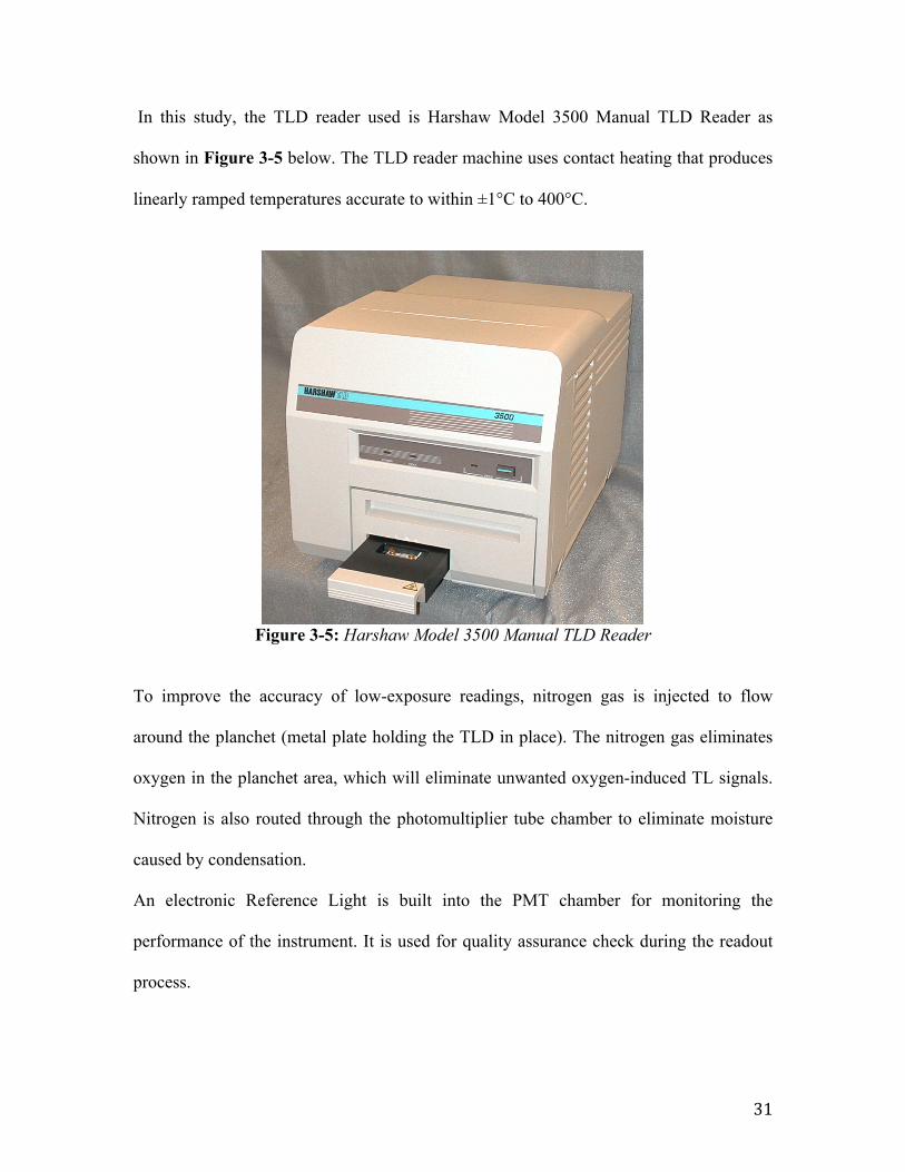
In this study, the TLD reader used is Harshaw Model 3500 Manual TLD Reader as

shown in Figure 3-5 below. The TLD reader machine uses contact heating that produces

linearly ramped temperatures accurate to within ±1°C to 400°C.

Figure 3-5: Harshaw Model 3500 Manual TLD Reader

To improve the accuracy of low-exposure readings, nitrogen gas is injected to flow

around the planchet (metal plate holding the TLD in place). The nitrogen gas eliminates

oxygen in the planchet area, which will eliminate unwanted oxygen-induced TL signals.

Nitrogen is also routed through the photomultiplier tube chamber to eliminate moisture

caused by condensation.

An electronic Reference Light is built into the PMT chamber for monitoring the

performance of the instrument. It is used for quality assurance check during the readout

process.

Model 3500 Manual TLD Reader with WinREMS3500-W-O-0805 Page 1-1

Operator’s Manual

Figure 1.1 Model 3500 Manual TLD Reader

1.0 System OverviewThe Harshaw Model 3500 Manual TLD

Reader is a PC-driven, manually-operated,tabletop instrument for thermoluminescentdosimetry (TLD) measurement. Iteconomically provides both high performanceand high reliability, and it complies with thelatest International Standards Organization(ISO) requirements. The 3500 reads onedosimeter per loading and accommodates avariety of TL configurations, including chips,disks, rods, and powder.

The system consists of two majorcomponents: the TLD Reader and theWindows Radiation Evaluation and Manage-ment System (WinREMS) software residenton a personal computer (PC), which isconnected to the Reader via a serialcommunications port .

1.1 TLD ReaderThe Reader's basic external components

include a front control panel consisting ofthree LED status lights and a Readpushbutton, a sample drawer assembly thatfeatures an interchangeable planchet and abuilt-in Reference Light for periodicmonitoring of Reader performance, and adrawer for neutral density filters. The rearpanel houses a voltage-selectable power inputmodule with fuse access, an instrument Resetbutton, a fitting for nitrogen gas tubing, anRS-232-C serial communication port, and arecessed pressure sensor adjusting screw.

The Reader uses contact heating with aclosed loop feedback system that produceslinearly ramped temperatures accurate towithin ±1o C to 400o C in the standard Reader,or 600o C with the High Temperature option.The Time Temperature Profile (TTP) is user-1.0 System Overview (cont’d)

  32  

3.1.4 TLD Glow Curve

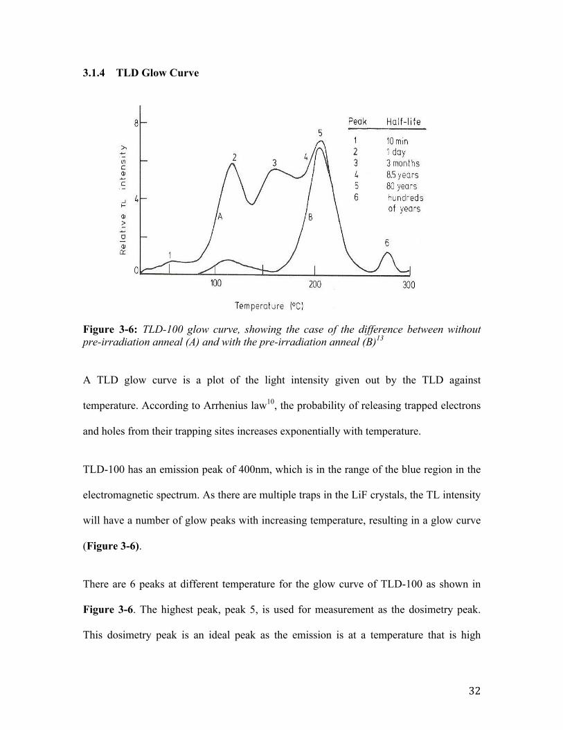
Figure 3-6: TLD-100 glow curve, showing the case of the difference between without pre-irradiation anneal (A) and with the pre-irradiation anneal (B)13

A TLD glow curve is a plot of the light intensity given out by the TLD against

temperature. According to Arrhenius law10, the probability of releasing trapped electrons

and holes from their trapping sites increases exponentially with temperature.

TLD-100 has an emission peak of 400nm, which is in the range of the blue region in the

electromagnetic spectrum. As there are multiple traps in the LiF crystals, the TL intensity

will have a number of glow peaks with increasing temperature, resulting in a glow curve

(Figure 3-6).

There are 6 peaks at different temperature for the glow curve of TLD-100 as shown in

Figure 3-6. The highest peak, peak 5, is used for measurement as the dosimetry peak.

This dosimetry peak is an ideal peak as the emission is at a temperature that is high

dose is the 5th peak. The dosimetry peak should have large enough temperature in

order not to be affected by the room temperature but also not to high in order not to be

affected by the black body emission of the TLD disc. The half-life of each peak is also

shown on figure 2.4.1.

Figure 2.4.1: Glow curve of TLD100 (A) – after pre-heating procedure (B) The half-lives of each

peak can also be seen. [4]

The problem is that at low temperatures the fading is high. Thus electrons

have enough energy to leave the traps and de-excite without the need of heat. That

affects the sensitivity of the dosimeter. It is possible to transfer the TL sensitivity of

low temperatures to the dosimetry peak by pre-heating just before the read-out. Thus

the background signal is removed and therefore, the dosimetry peak is much more

distinct (figure 2.4.1-curve B).

After the TLDs are read-out, they are annealed in order to ensure the signal

has been completely removed and the TLD is again ready for use. For the TLD100

the annealing is not as simple, as it is first heated at 4000C for an hour and then at

800C for 16 to 24 hours. If the used annealing temperature is more than 4000C the

sensitivity of the material is reduced [4].

The area under the glow curve, after the appropriate calibration, corresponds

to the absorbed dose which is measured using the TLD reader. If the rate of the

9

  33  

enough, so that it is not affected by room temperatures, and low enough, so that it is not

influenced by the TLD’s black body emission. Unlike the other peaks, fading of peak 5 is

slow as it has a long half-life, which is ideal for measurement, as shown in Figure 3-6.

At low temperatures, electrons may gain enough energy to escape the trapping sites and

de-excite without much increase in temperature. This causes a problem, as it will affect

the sensitivity of the dosimeter. The solution is to remove the peaks at low temperatures

by pre-heating the TLDs before readout. This pre-heating also removes the background

signal, resulting the dosimetry peak (peak 5) to be much more distinct as shown in

Figure 3-6 (curve B)

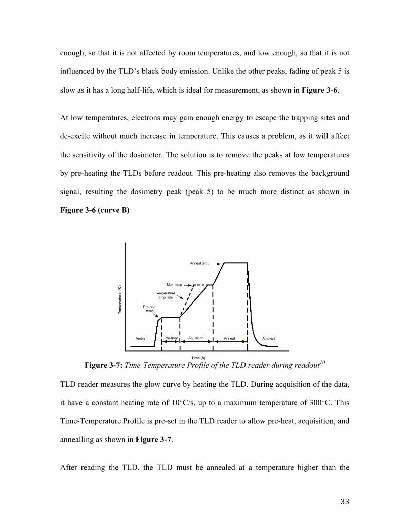
Figure 3-7: Time-Temperature Profile of the TLD reader during readout10  TLD reader measures the glow curve by heating the TLD. During acquisition of the data,

it have a constant heating rate of 10°C/s, up to a maximum temperature of 300°C. This

Time-Temperature Profile is pre-set in the TLD reader to allow pre-heat, acquisition, and

annealling as shown in Figure 3-7.

After reading the TLD, the TLD must be annealed at a temperature higher than the

TLD MaterialDOSM-0-N-1202-001 Page 1

Standard TTP Recommendations1 IntroductionThis technical notice consists ofHarshaw standard Time TemperatureProfile Recommendation tables for thefollowing TLD materials:

TLD Material See TableTLD-100; LiF:Mg,Ti 1TLD-100H; LiF:Mg,Cu, P 2TLD-200; CaF2:Dy 3TLD-300; CaF2:Tm 4TLD-400; CaF2:Mn 5TLD-500; Al2O3:C 6TLD-600; 6LiF:Mg,Ti 7TLD-600H; 6LiF:Mg,Cu, P 8TLD-700; 7LiF:Mg,Ti 9TLD-700H; 7LiF:Mg,Cu, P 10TLD-800; Li2B4O7:Mn 11TLD-900; CaSO4:Dy 12

Use these tables when setting up yourTime Temperature profile for yourappropriate TLD material and Reader.

The typical Time-Temperature Profile(TTP) diagram is shown in Figure 1. Theheating cycle normally consists ofPreheat, Acquisition, Anneal, and Coolsegments. Preheat is applied to segregatethe light generated from low-energytraps to minimize fade effect.Dosimetrically significant data aregenerated and stored during theAcquisition segment. To ensure currentexposures do not contribute tosubsequent measurements, the Annealcycle is applied. This has the effect ofremoving signal residual. The heatingcycle applied helps to establish thereproducibility of the dosimeter.

Figure 1 Typical Time-Temperature Profile (TTP) Diagram

  34  

readout temperature (400°C for 1 hour and 100°C for 3 hours for TLD-100). This

annealing process releases any trapped electrons and holes that are not released during

readout so that the TLD could be reused for subsequent measurements.

3.1.5 TLD setup for radiotherapy

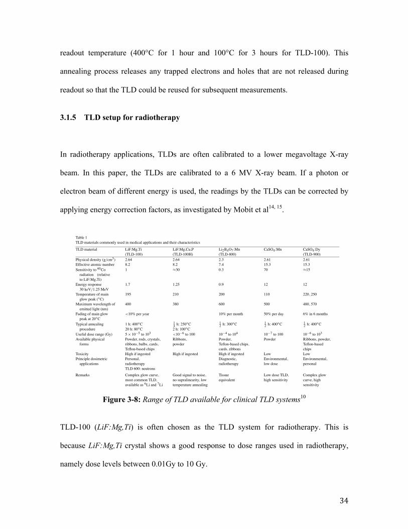
In radiotherapy applications, TLDs are often calibrated to a lower megavoltage X-ray

beam. In this paper, the TLDs are calibrated to a 6 MV X-ray beam. If a photon or

electron beam of different energy is used, the readings by the TLDs can be corrected by

applying energy correction factors, as investigated by Mobit et al14, 15.

Figure 3-8: Range of TLD available for clinical TLD systems10

TLD-100 (LiF:Mg,Ti) is often chosen as the TLD system for radiotherapy. This is

because LiF:Mg,Ti crystal shows a good response to dose ranges used in radiotherapy,

namely dose levels between 0.01Gy to 10 Gy.

ApplicationsofThermolum

inescentDosim

etersinMedicine

417

Table 1TLD materials commonly used in medical applications and their characteristics

TLD material LiF:Mg,Ti LiF:Mg,Cu,P Li2B4O7:Mn CaSO4:Mn CaSO4:Dy(TLD-100) (TLD-100H) (TLD-800) (TLD-900)

Physical density (g/cm3) 2.64 2.64 2.3 2.61 2.61Effective atomic number 8.2 8.2 7.4 15.3 15.3Sensitivity to 60Coradiation (relativeto LiF:Mg,Ti)

1 !30 0.3 70 !15

Energy response30 keV/1.25 MeV

1.7 1.25 0.9 12 12

Temperature of mainglow peak ("C)

195 210 200 110 220, 250

Maximum wavelength ofemitted light (nm)

400 380 600 500 480, 570

Fading of main glowpeak at 20"C

<10% per year 10% per month 50% per day 6% in 6 months

Typical annealing 1 h: 400"C 14 h: 250

"C 12 h: 300

"C 12 h: 400

"C 12 h: 400

"Cprocedure 20 h: 80"C 2 h: 100"C

Useful dose range (Gy) 5# 10$5 to 103 <10$6 to 100 10$4 to 104 10$7 to 100 10$6 to 103Available physicalforms

Powder, rods, crystals,ribbons, bulbs, cards,Teflon-based chips

Ribbons,powder

Powder,Teflon-based chips,cards, ribbons

Powder Ribbons, powder,Teflon-basedchips

Toxicity High if ingested High if ingested High if ingested Low LowPrinciple dosimetricapplications

Personal,radiotherapyTLD 600: neutrons

Diagnostic,radiotherapy

Environmental,low dose

Environmental,personal

Remarks Complex glow curve,most common TLD,available as 6Li and 7Li

Good signal to noise,no supralinearity, lowtemperature annealing

Tissueequivalent

Low dose TLD,high sensitivity

Complex glowcurve, highsensitivity

Selected references Cameron et al., 1961;Mansfield, 1976;Horowitz, 1990, 1993;Kron et al., 1993

Zha et al., 1993;Horowitz, 1993

Horowitz et al., 1980;Horowitz, 1981, 1984

Bjarngard et al.,1976

Yamashita et al., 1971;Horowitz, 1984

  35  

As shown in Figure 3-2, each TLD is specific and is issued an identification, which is

marked by an alphabet (e.g. A,B,C,D,…) and a number (1 to 10), indicated on the

aluminum or plastic tray.

Quality assurance checks are done for the TLDs in order to select the reliable TLDs for

dosimetric experiments. These initial checks includes the following considerations:

• Visual check of any TLDs with chipped corners and discolouration

• TLD response uniformity

• TLD glow curves

• TLD reading reproducibility

• TLD linearity and supralinearity readings

It is important to examine the dose response for TLDs in radiation therapy applications.

In high precision applications, it is necessary to recalibrate the TLD before each

measurement. The operation procedure in handling the TLDs is shown in the diagram

below.

  36  

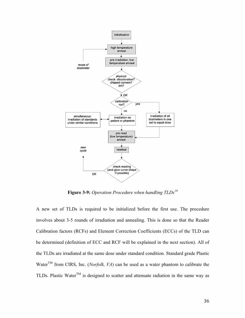
Figure 3-9: Operation Procedure when handling TLDs16

A new set of TLDs is required to be initialized before the first use. The procedure

involves about 3-5 rounds of irradiation and annealing. This is done so that the Reader

Calibration factors (RCFs) and Element Correction Coefficients (ECCs) of the TLD can

be determined (definition of ECC and RCF will be explained in the next section). All of

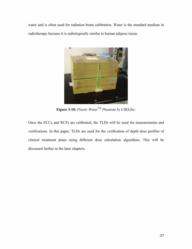
the TLDs are irradiated at the same dose under standard condition. Standard grade Plastic

WaterTM from CIRS, Inc. (Norfolk, VA) can be used as a water phantom to calibrate the

TLDs. Plastic WaterTM is designed to scatter and attenuate radiation in the same way as

422 P.N. Mobit and T. Kron

Fig. 5. Flow diagram illustrating the use of TL dosimeters.

The typical read-out procedure involves a pre-read anneal, which empties low energytraps, thereby reducing errors introduced by the fading of the TL signal. For LiF:Mg,Ti atypical pre-read anneal involves heating the detector to a temperature of 150!C and main-taining this temperature for 10 s. The details of the read-out procedure are somewhat arbi-trary and depend on the parameters of TL signal to be evaluated. In general, it is sufficientto determine the area under glow peaks IV and V of LiF:Mg,Ti to achieve the accuracy andreliability required for clinical dosimetry. In this case a stepped heating process is adequatein which the dosimeters are heated to 270!C for at least 10 s. It is worthwhile mentioningthat the heating rate employed to heat the samples to 270!C can affect the summed lightintensity of peaks IV and V due to a process called thermal quenching.

  37  

water and is often used for radiation beam calibration. Water is the standard medium in

radiotherapy because it is radiologically similar to human adipose tissue.

Figure 3-10: Plastic WaterTM Phantom by CIRS,Inc.

Once the ECCs and RCFs are calibrated, the TLDs will be used for measurements and

verifications. In this paper, TLDs are used for the verification of depth dose profiles of

clinical treatment plans using different dose calculation algorithms. This will be

discussed further in the later chapters.

  38  

3.2 TLD measurement methods

3.2.1 Element Correction Coefficient

TLDs may differ from one another in terms of Thermoluminesence Efficiency (where

Thermoluminenesce Efficiency (TLE) is defined as the emitted TL light intensity per unit

of absorbed dose). This can be corrected by calculating the individual Element

Correction Coefficients (ECCs) for each TLD. By applying ECCs, the spread of TLE will

be reduced from 10-15% to a low percentage of 1-2%.17

The ECC could be calculated by relating the TLE of each TLD of the sample TLD

population (called Field Dosimeters) to the average TLE of a small subset of the sample

TLD population that is used for calibration (called Calibration Dosimeters). The ECC

will correct the TLE of the Field Dosimeters to the mean value of the Calibration

Dosimeters group, accounting for any response difference between TLDs.

  39  

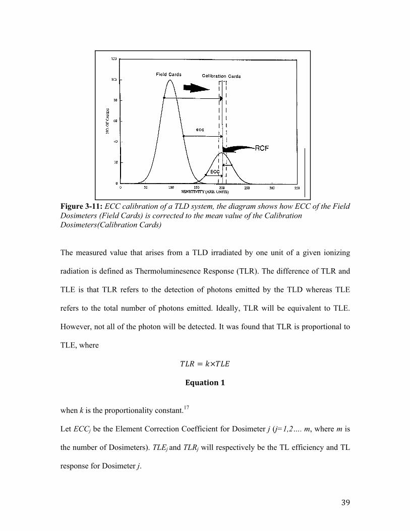
Figure 3-11: ECC calibration of a TLD system, the diagram shows how ECC of the Field Dosimeters (Field Cards) is corrected to the mean value of the Calibration Dosimeters(Calibration Cards)

The measured value that arises from a TLD irradiated by one unit of a given ionizing

radiation is defined as Thermoluminesence Response (TLR). The difference of TLR and

TLE is that TLR refers to the detection of photons emitted by the TLD whereas TLE

refers to the total number of photons emitted. Ideally, TLR will be equivalent to TLE.

However, not all of the photon will be detected. It was found that TLR is proportional to

TLE, where

𝑇𝐿𝑅 = 𝑘×𝑇𝐿𝐸

Equation  1  

when k is the proportionality constant.17

Let ECCj be the Element Correction Coefficient for Dosimeter j (j=1,2…. m, where m is

the number of Dosimeters). TLEj and TLRj will respectively be the TL efficiency and TL

response for Dosimeter j.

Harshaw Dosimetry SystemALGM-0-C-0398 Page 29

System Calibration Procedure

Figure 9Internal Calibration of a TLD System

7.0 Calibration Methodology (cont'd)7.1 Element Correction Coefficients(cont'd)

Note that the ECC values for the FieldDosimeters would have been the same hadthey been generated at the same time as theCalibration Dosimeters' ECCs or at any othertime since the C values from (10) and (11)would have been canceled out in (12).

Once ECCs for the Field Dosimeters havebeen generated and applied, their TL efficiency(sensitivity) is virtually equal to the mean TLefficiency of the Calibration Dosimeters, and,as a result, all the dosimeter population willhave virtually the same TL efficiency, asshown in Figure 9. When new dosimeters areadded to the population, their TL efficiencycan be set to be virtually equal to the existingdosimeter population by generating ECCs forthe new dosimeters. The only parameterwhich must remain constant is the inherentsensitivity of the Calibration Dosimeters that

are being used. Extensive testing by BICRONand by our customers has shown, however,that the TL dosimeters used here can besubjected to hundreds of reuse cycles withoutany noticeable change in their TL efficiency.

Note that the radiation source used forgenerating the ECCs for the Field Dosimetersdoes not have to be the same one used forgenerating the ECCs for the CalibrationDosimeters, provided that a subset ofCalibration Dosimeters is exposed to the sameradiation field as the Field Dosimeters whoseECCs are being generated. Also note thatthere is no need for the dosimeters to bemounted in their holders during irradiation,since the only purpose of this irradiation is toinduce an excitation in the TL material, whichwill result in a measurable TL signal that isproportional to the TL efficiency of the TLdosimeter. Furthermore, no attempt has beenmade yet to correlate this TL response to anykind of "real" dose units.

  40  

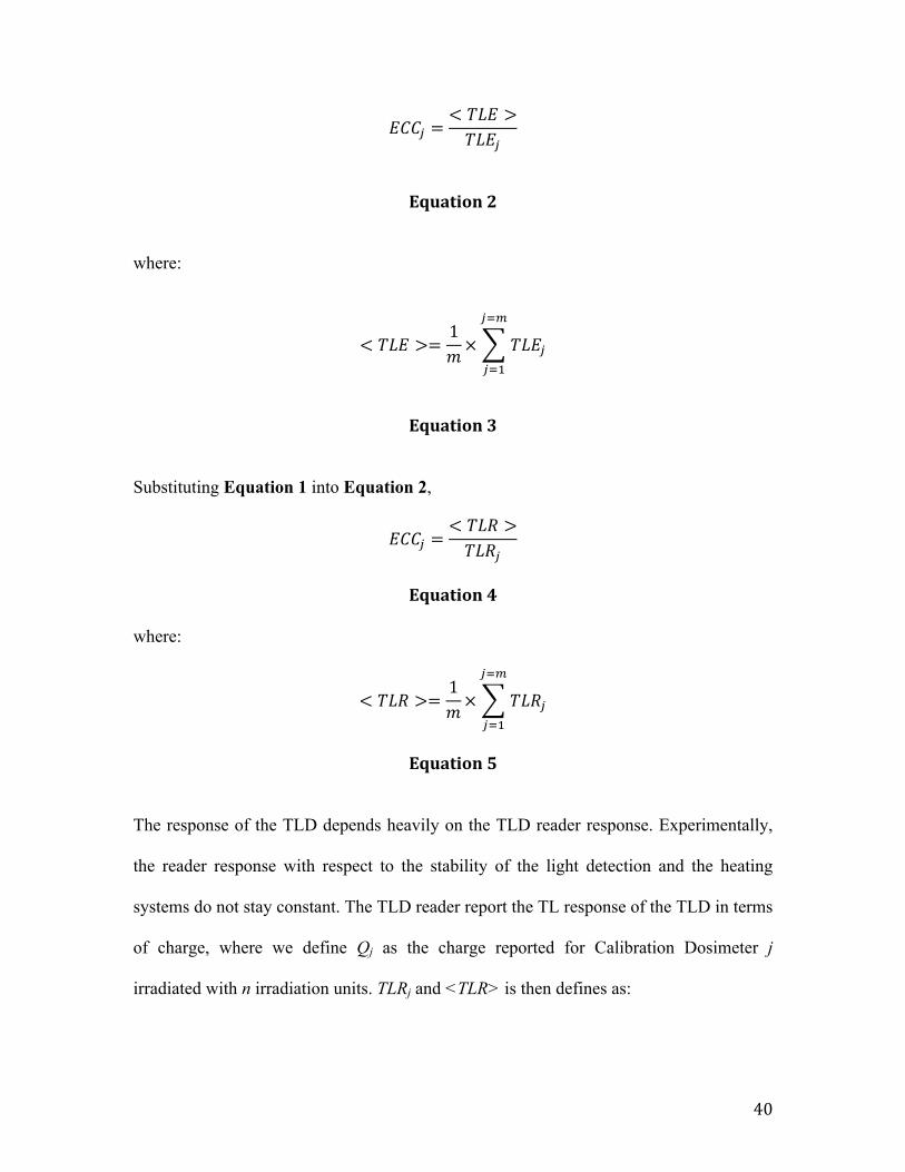
𝐸𝐶𝐶! =< 𝑇𝐿𝐸 >𝑇𝐿𝐸!

Equation  2  

where:

< 𝑇𝐿𝐸 >=1𝑚× 𝑇𝐿𝐸!

!!!

!!!

Equation  3  

Substituting Equation 1 into Equation 2,

𝐸𝐶𝐶! =< 𝑇𝐿𝑅 >𝑇𝐿𝑅!

Equation  4    

where:

< 𝑇𝐿𝑅 >=1𝑚× 𝑇𝐿𝑅!

!!!

!!!

Equation  5  

The response of the TLD depends heavily on the TLD reader response. Experimentally,

the reader response with respect to the stability of the light detection and the heating

systems do not stay constant. The TLD reader report the TL response of the TLD in terms

of charge, where we define Qj as the charge reported for Calibration Dosimeter j

irradiated with n irradiation units. TLRj and <TLR> is then defines as:

  41  

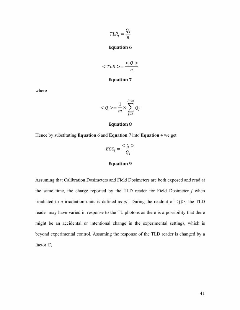
𝑇𝐿𝑅! =𝑄!𝑛

Equation  6  

< 𝑇𝐿𝑅 >=< 𝑄 >𝑛

Equation  7    

where

< 𝑄 >=1𝑚× 𝑄!

!!!

!!!

Equation  8    

Hence by substituting Equation 6 and Equation 7 into Equation 4 we get

𝐸𝐶𝐶! =< 𝑄 >𝑄!

Equation  9  

Assuming that Calibration Dosimeters and Field Dosimeters are both exposed and read at

the same time, the charge reported by the TLD reader for Field Dosimeter j when

irradiated to n irradiation units is defined as qj´. During the readout of <Q>, the TLD

reader may have varied in response to the TL photons as there is a possibility that there

might be an accidental or intentional change in the experimental settings, which is

beyond experimental control. Assuming the response of the TLD reader is changed by a

factor C,

   

  42  

< 𝑄 > ´ = C  ×  < 𝑄 >

Equation  10    

and

𝑞!´ = C  ×  𝑞!

Equation  11  

where qj is the unchanged charge of Field Dosimeter j and <Q>´ is the average reported

charge of the Calibrated Dosimeters under the new changed environmental settings.

Hence, by substituting Equation 10 and Equation 11 we see that

𝐸𝐶𝐶! =< 𝑄 > ´𝑞´!

Equation  12  

3.2.2 Reader Calibration Factor and Absorbed Dose

In order to convert TL photons to measurable electric signals (in terms of charge), the

ratio between the average TL response of the Calibration Dosimeters and the irradiated

radiation quantity L can be found. This ratio is defined as Reader Calibration Factor

(RCF). It will account for the conditions of the experimental settings during

measurement, correcting for any stochastic changes in the experiment. It also acts as the

main link between the TL response in terms of charge and the absorbed dose, D, in terms

of Gray.

  43  

𝑅𝐶𝐹 =< 𝑄 >𝐷

Equation  13  

To accurately obtain the RCF, it is important to reproduce the readings of the Calibration

Dosimeters by periodically calibrating it to sources that are traceable to recognized

absorbed dose standards. By substituting Equation 13 into Equation 12

𝐸𝐶𝐶! =𝑅𝐶𝐹×𝐿𝑞!

Equation  14    And hence, the dose response for Dosimeter j will be

𝐷! =𝑞!×𝐸𝐶𝐶!𝑅𝐶𝐹

Equation  15  

  44  

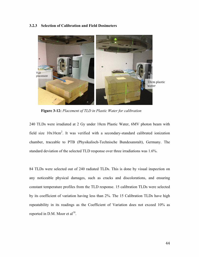
3.2.3 Selection of Calibration and Field Dosimeters

Figure 3-12: Placement of TLD in Plastic Water for calibration

240 TLDs were irradiated at 2 Gy under 10cm Plastic Water, 6MV photon beam with

field size 10x10cm2. It was verified with a secondary-standard calibrated ionization

chamber, traceable to PTB (Physikalisch-Technische Bundesanstalt), Germany. The

standard deviation of the selected TLD response over three irradiations was 1.6%.

84 TLDs were selected out of 240 radiated TLDs. This is done by visual inspection on

any noticeable physical damages, such as cracks and discolorations, and ensuring

constant temperature profiles from the TLD response. 15 calibration TLDs were selected

by its coefficient of variation having less than 2%. The 15 Calibration TLDs have high

repeatability in its readings as the Coefficient of Variation does not exceed 10% as

reported in D.M. Moor et al18.

TLD  placement  

10cm  plastic  water  

  45  

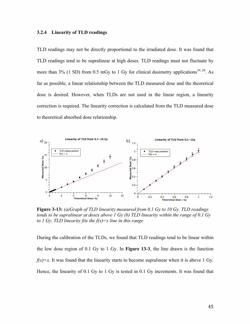
3.2.4 Linearity of TLD readings

 TLD readings may not be directly proportional to the irradiated dose. It was found that

TLD readings tend to be supralinear at high doses. TLD readings must not fluctuate by

more than 3% (1 SD) from 0.5 mGy to 1 Gy for clinical dosimetry applications19, 20. As

far as possible, a linear relationship between the TLD measured dose and the theoretical

dose is desired. However, when TLDs are not used in the linear region, a linearity

correction is required. The linearity correction is calculated from the TLD measured dose

to theoretical absorbed dose relationship.

Figure 3-13: (a)Graph of TLD linearity measured from 0.1 Gy to 10 Gy. TLD readings tends to be supralinear at doses above 1 Gy (b) TLD linearity within the range of 0.1 Gy to 1 Gy. TLD linearity fits the f(x)=x line in this range

During the calibration of the TLDs, we found that TLD readings tend to be linear within

the low dose region of 0.1 Gy to 1 Gy. In Figure 13-3, the line drawn is the function

f(x)=x. It was found that the linearity starts to become supralinear when it is above 1 Gy.

Hence, the linearity of 0.1 Gy to 1 Gy is tested in 0.1 Gy increments. It was found that

a)   b)  

  46  

TLD measurements deviated from linearity by less than 3%. The results found are

consistent as reported in several studies19-21.

  47  

3.3 Summary

To summarize the theoretical framework of TLDs, we will need to have several

considerations.

Firstly, we have to recognize the advantages and disadvantages of having a TLD

dosimetric system. It is possible to obtain optimum measurement capability when TLDs

are applied for the appropriate dosimetric application.

TLDs are lithium fluoride crystals that are doped, in the case of TLD-100, with

magnesium and titanium. This creates trapping sites for excited electrons when TLD is

irradiated. During readout, these electrons de-excite and releases excess energy as light.

This response of the TLD is proportional to the dose absorbed and can be read using a

TLD reader.

TLD reader reads the TLD measurements in a plot of TL intensity against temperature,

which is known as the glow curve. The dosimetry peak of the glow curve will be the TL

response.

Calibration and Field dosimeters were chosen by visual inspection, their response values

and temperature profiles. The selection of TLDs allows proper calibration for high

precision measurement.

  48  

During calibration, the ECCs and the RCFs of the TLDs are determined. ECC corrects

the Thermoluminesence Efficiency differences between TLDs, where as RCF corrects

stochastic errors between each round of measurement.

Lastly, it was found that TL response is linear at dose region 0.1Gy to 1 Gy. Above 1 Gy,

linearity correction is required.

  49  

4 Dose Calculation Algorithms

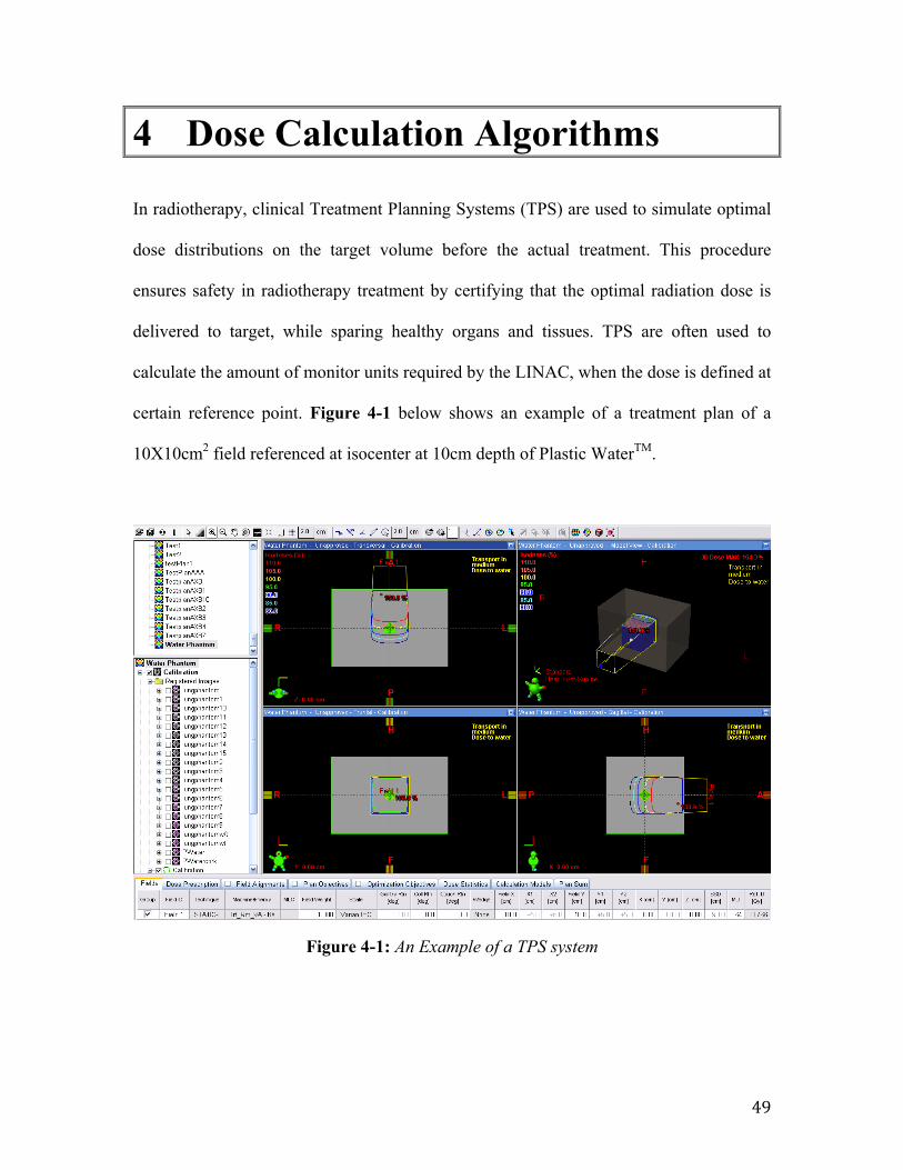
In radiotherapy, clinical Treatment Planning Systems (TPS) are used to simulate optimal

dose distributions on the target volume before the actual treatment. This procedure

ensures safety in radiotherapy treatment by certifying that the optimal radiation dose is

delivered to target, while sparing healthy organs and tissues. TPS are often used to

calculate the amount of monitor units required by the LINAC, when the dose is defined at

certain reference point. Figure 4-1 below shows an example of a treatment plan of a

10X10cm2 field referenced at isocenter at 10cm depth of Plastic WaterTM.

Figure 4-1: An Example of a TPS system

  50  

Modern TPS uses advanced dose calculation algorithms to calculate the dose

distributions in heterogeneous medium. Based on the calculation algorithm used, the

accuracy and the amount of time taken to generate the dose distribution will vary.

Currently, the golden standard for dose calculation algorithm is by Monte Carlo (MC)

calculations1, 3-5, 22. However, due to the complexity of modern radiotherapy, the

calculation time required by MC is significant and thus may not be suitable for clinical

use.

There is an increasing demand on dose calculation accuracy for treatment planning

optimization for heterogeneous medium. Hence, one of the current clinical dose

calculation algorithm is the Anistropic Analytical Algorithm (AAA)5, 23-27, which is

efficient and sufficiently accurate to be used clinically.

Since 2008, Transpire Inc. wrote a new dose calculation algorithm known as Acuros

XBTM, to improve the efficiency and accuracy for radiotherapy applications1, 2, 5, 28-30. We

will further investigate both AAA and Acuros XB further below. The validation of both

algorithms with TLDs will be done in the subsequent chapter.

  51  

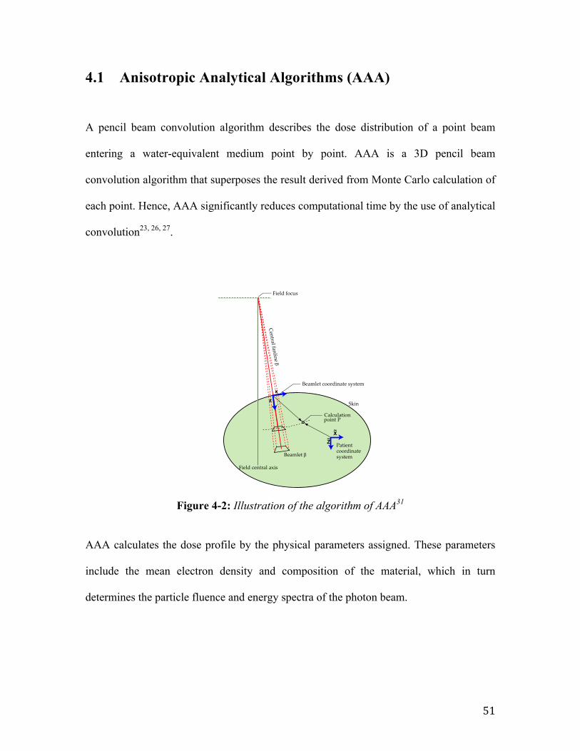
4.1 Anisotropic Analytical Algorithms (AAA)

A pencil beam convolution algorithm describes the dose distribution of a point beam

entering a water-equivalent medium point by point. AAA is a 3D pencil beam

convolution algorithm that superposes the result derived from Monte Carlo calculation of

each point. Hence, AAA significantly reduces computational time by the use of analytical

convolution23, 26, 27.

Figure 4-2: Illustration of the algorithm of AAA31

AAA calculates the dose profile by the physical parameters assigned. These parameters

include the mean electron density and composition of the material, which in turn

determines the particle fluence and energy spectra of the photon beam.

100 Eclipse Algorithms Reference Guide

Figure 13 Coordinates in Patient Coordinate System and Beamlet Coordinate System on X–Z Plane

TheȱbroadȱclinicalȱbeamȱisȱdividedȱintoȱfiniteȬsizeȱbeamletsȱE.ȱTheȱsideȱlengthȱofȱtheȱbeamletȱcorrespondsȱtoȱtheȱresolutionȱofȱtheȱcalculationȱgridȱonȱtheȱisocenterȱplane.

TheȱdoseȱcalculationȱisȱbasedȱonȱtheȱconvolutionsȱoverȱtheȱbeamletȱcrossȬsectionsȱseparatelyȱforȱtheȱprimaryȱphotons,ȱextraȬfocalȱphotonsȱ(secondȱsource),ȱscatterȱfromȱhardȱwedges,ȱandȱforȱelectronsȱcontaminatingȱtheȱprimaryȱbeam.ȱTheȱdoseȱisȱconvolvedȱbyȱusingȱtheȱphysicalȱparametersȱdefinedȱforȱeveryȱbeamletȱE.

AllȱdepthȬdependentȱfunctionsȱusedȱinȱtheȱbeamletȱconvolutionsȱareȱcomputedȱalongȱtheȱcentralȱfanlineȱofȱtheȱbeamletȱusingȱtheȱdepthȱcoordinateȱz.ȱLateralȱdoseȱscatteringȱdueȱtoȱphotonsȱandȱelectronsȱisȱdefinedȱonȱtheȱsphericalȱshellȱperpendicularȱtoȱtheȱcentralȱfanlineȱofȱtheȱbeamlet.ȱTheȱAAAȱmakesȱtheȱassumptionȱthatȱtheȱdoseȱresultingȱ

Fieldȱfocus

Skin

BeamletȱE

Fieldȱcentralȱaxis

Beamletȱcoordinateȱsystem

Patientcoordinatesystem

Centralȱfanline�E

x

Z

X

z

~

~

CalculationpointȱP

  52  

AAA approximates the broad clinical beam by dividing it into finite‐size beamlets as

shown in Figure 4-2. The length of the beamlet is determined by the resolution of the

calculation grid on the isocenter plane.

Therefore, the calculation is determined by the convolution of the interaction for every

beamlet. The central fanline of the beamlet is the source where all depth‐dependent

functions are computed. A modeled spherical shell perpendicular to the central fanline of

the beamlet approximates lateral dose scattering due to photons.31

Currently, AAA is used as the clinical dose calculation algorithm in National Cancer

Center Singapore. This dose algorithm has been validated and concluded that it has good

agreement between calculated and measured dose data with deviations smaller than 1%

for standard field sizes (10x10cm2)24.

  53  

4.2 Acuros External Beam (AXB)

Radiotherapy dose calculations can also be determined accurately using deterministic

solutions to the coupled system of linear Boltzmann transport equations (LBTEs)32-35.

The coupled system of LBTEs can be solved stochastically by Monte Carlo methods

using information from its particle histories. The second method is to use grid-based

LBTE solution methods by implementing discretization of photon and electron fluences

in space, energy, and angle so as to allow a deterministic solution of the transport of

radiation through matter. Through this second method, Attila® (Transpire Inc.) have

developed a new dose calculation algorithm so as to achieve both efficiency and

accuracy, and modify it specifically for radiotherapy applications. Acuros XBTM

algorithm (Transpire Inc.) has recently been implemented by Varian Medical Systems in

the Eclipse Treatment Planning Systems and was recently released for clinical dose

calculations.

Vassiliev et al35 investigated the accuracy of the AXB by comparing it with Monte Carlo

calculations36. Their study found an excellent ±2% agreement in depth dose profiles

through a heterogeneous unit density phantom and ±2% agreement in 99.9% of voxels.

Bush et al30 have concluded that AXB algorithm is capable of modeling radiotherapy

dose deposition with accuracy that is comparable to Monte Carlo.

In external photon beam radiotherapy, AXB is able to accurately account for the effects

of heterogeneities such as lung tissue, air, bone and other implants may significantly

  54  

influence the dose distribution in the patient, especially in the presence of small or

irregular fields.

4.2.1 Computed Tomography (CT) number – mass density relationship

The fundamental data used by AXB are macroscopic atomic cross sections. A

macroscopic cross section is the probability that an interaction will occur per unit path

length of particle travel. Macroscopic cross sections are composed from two values: the

interaction’s microscopic cross section and the mass density of the material.

In order to perform a calculation, AXB must know the macroscopic cross section of each

element in its computational grid. The treatment planning system provides AXB with a

mass density and material type in each voxel of the image grid by referring to a CT

Calibration Curve. A CT calibration curve relates the CT number of the material with the

material’s density. Hence, it is essential to calibrate and derive a CT calibration curve

accurately for AXB dose calculation.

X-ray Computed Tomography measures the attenuation of x-ray beams passing through

sections of a body through different angles. By having these measurements, the CT is

able to reconstruct the body virtually. For each given pixel, the CT determines a relative

linear attenuation coefficient, µeff (r), for each spatial coordinate. It is then normalized to

the linear attenuation coefficient of the reference material, water37-39.

  55  

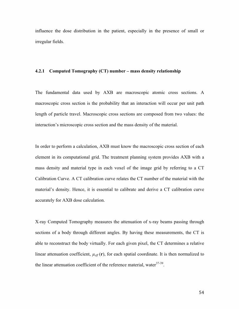
𝐻𝑈 𝒓 =𝜇!"" 𝒓 − 𝜇!""

!!!

𝜇!""!!! −  𝜇!""!"#

Equation 16

CT numbers are known as Hounsfield Units (HU) 37 as shown in Equation 16 above. By

obtaining the HU of different materials of known densities and chemical compositions,

the CT calibration curve can be determined.

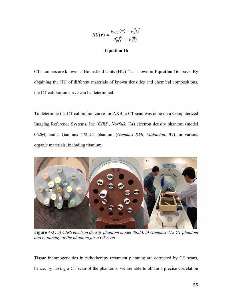
To determine the CT calibration curve for AXB, a CT scan was done on a Computerized

Imaging Reference Systems, Inc (CIRS , Norfolk, VA) electron density phantom (model

062M) and a Gammex 472 CT phantom (Gammex RMI, Middleton, WI) for various

organic materials, including titanium.

Figure 4-3: a) CIRS electron density phantom model 062M, b) Gammex 472 CT phantom and c) placing of the phantom for a CT scan

Tissue inhomogeneities in radiotherapy treatment planning are corrected by CT scans,

hence, by having a CT scan of the phantoms, we are able to obtain a precise correlation

a)   b)   c)  

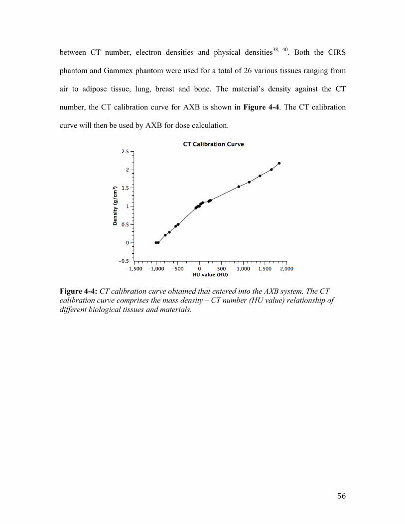
  56  

between CT number, electron densities and physical densities38, 40. Both the CIRS

phantom and Gammex phantom were used for a total of 26 various tissues ranging from

air to adipose tissue, lung, breast and bone. The material’s density against the CT

number, the CT calibration curve for AXB is shown in Figure 4-4. The CT calibration

curve will then be used by AXB for dose calculation.

Figure 4-4: CT calibration curve obtained that entered into the AXB system. The CT calibration curve comprises the mass density – CT number (HU value) relationship of different biological tissues and materials.

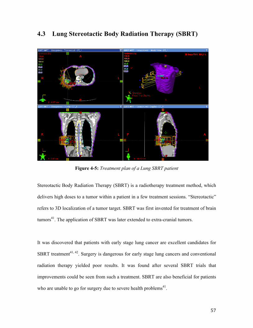
  57  

4.3 Lung Stereotactic Body Radiation Therapy (SBRT)

Figure 4-5: Treatment plan of a Lung SBRT patient

Stereotactic Body Radiation Therapy (SBRT) is a radiotherapy treatment method, which

delivers high doses to a tumor within a patient in a few treatment sessions. “Stereotactic”

refers to 3D localization of a tumor target. SBRT was first invented for treatment of brain

tumors41. The application of SBRT was later extended to extra-cranial tumors.

It was discovered that patients with early stage lung cancer are excellent candidates for

SBRT treatment41, 42. Surgery is dangerous for early stage lung cancers and conventional

radiation therapy yielded poor results. It was found after several SBRT trials that

improvements could be seen from such a treatment. SBRT are also beneficial for patients

who are unable to go for surgery due to severe health problems41.

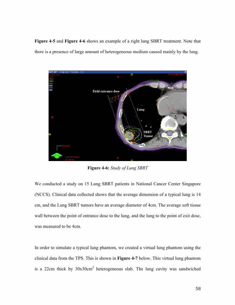
  58  

Figure 4-5 and Figure 4-6 shows an example of a right lung SBRT treatment. Note that

there is a presence of large amount of heterogeneous medium caused mainly by the lung.

Figure 4-6: Study of Lung SBRT

We conducted a study on 15 Lung SBRT patients in National Cancer Center Singapore

(NCCS). Clinical data collected shows that the average dimension of a typical lung is 14

cm, and the Lung SBRT tumors have an average diameter of 4cm. The average soft tissue

wall between the point of entrance dose to the lung, and the lung to the point of exit dose,

was measured to be 4cm.

In order to simulate a typical lung phantom, we created a virtual lung phantom using the

clinical data from the TPS. This is shown in Figure 4-7 below. This virtual lung phantom

is a 22cm thick by 30x30cm2 heterogeneous slab. The lung cavity was sandwiched

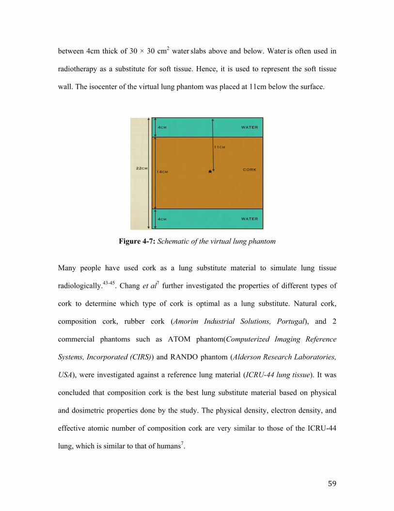
  59  

between 4cm thick of 30 × 30 cm2 water slabs above and below. Water is often used in

radiotherapy as a substitute for soft tissue. Hence, it is used to represent the soft tissue

wall. The isocenter of the virtual lung phantom was placed at 11cm below the surface.

Figure 4-7: Schematic of the virtual lung phantom

Many people have used cork as a lung substitute material to simulate lung tissue

radiologically.43-45. Chang et al7 further investigated the properties of different types of

cork to determine which type of cork is optimal as a lung substitute. Natural cork,

composition cork, rubber cork (Amorim Industrial Solutions, Portugal), and 2

commercial phantoms such as ATOM phantom(Computerized Imaging Reference

Systems, Incorporated (CIRS)) and RANDO phantom (Alderson Research Laboratories,

USA), were investigated against a reference lung material (ICRU-44 lung tissue). It was

concluded that composition cork is the best lung substitute material based on physical

and dosimetric properties done by the study. The physical density, electron density, and

effective atomic number of composition cork are very similar to those of the ICRU-44

lung, which is similar to that of humans7.

Isocenter set at 11cm below Surface

lung - 14cm Water - 4cm

PDD measurment:2cm before interfaceat interface2cm after interfaceIsocenter

0.01cm3 water

MEASUREMENTS

22cm

4cm

4cm

14cm

11cm

WATER

WATER

CORK

Wednesday, March 6, 13

  60  

Figure 4-8: Result showing composite cork having similar dosimetric properties to lung tissue standard, ICRU-447.

Therefore, composite cork was used to simulate the lung cavity in this study. The lung

cavity was simulated virtually in the TPS by using composite cork material with physical

density 0.27g/cm3 and CT number -743, as reported by Chang et al7.

With the virtual phantom, a physical lung phantom was built by having a composite cork

cavity sandwiched between 4cm thick of 30 × 30 cm2 Plastic WaterTM slabs above and

below as shown in Figure 4-9. The composite cork material used was 14 pieces of 15 ×

15cm2 1cm thick slabs. The density of the composite cork material was measured and

verified to be 0.27 g/cm3.

composition cork results are used here to represent a known(C%, H%, O%) of lung material. Other lung simulationmaterials may be used to compare other factors (e.g., EDG)and how they will alter the dosimetric characteristics. This

will be further explained in Sec. IV. In Fig. 3(b), it is explicitthat there is negligible effect from physical density on thelarger field size. Other lung materials exhibited an analogoustrend. In an effort to determine if factors other than the phys-ical density affected the dosimetric characteristics, we fixedthe physical density value at 0.26 g/cm3 (identical to ICRU-44 lung) for each of the test materials; the results are shownin Fig. 4. The PDD curve of all materials for all field sizeswere lower than ICRU-44 lung; however, the RANDO lungwas the lowest. By comparing physical properties fromTable I, it is concluded that this is due to the lower EDG ofthe test materials (3.18! 1023 electrons/g for RANDO, and3.23–3.25! 1023 electrons/g for others) than that of theICRU-44 lung (3.35! 1023 electrons/g).

The hydrogen atom has an electron density nearly twicethat of other atoms. As seen in Table I, the weight fraction ofthe hydrogen of the ICRU-44 is 10.3% compared to 5.74%of RANDO and 7.69%–8.45% of the other materials. We

FIG. 2. Percentage depth dose (PDD) of the water-lung materials-water con-figuration per Fig. 1; Field sizes for (a) 1! 1 cm2 (b) 10! 10 cm2, and (c)dose differences (%) of lung substitutes (compared to ICRU-44 lung) atZ" 5 cm for various field sizes.

FIG. 3. PDD curves for various simulated physical densities (0.15–0.3 g =cm3)of the composition cork, for field sizes (a) 1! 1cm2 and (b) 10! 10 cm2.

2017 Chang et al.: Comparison of cork and others as lung substitutes 2017

Medical Physics, Vol. 39, No. 4, April 2012

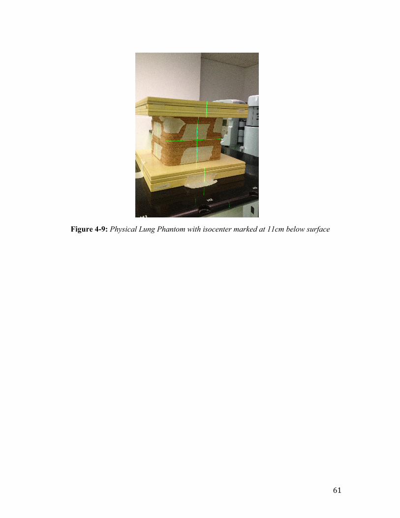
  61  

Figure 4-9: Physical Lung Phantom with isocenter marked at 11cm below surface

  62  

4.4 Summary

In summary, several dose calculation algorithms and its concepts are highlighted in this

chapter. Treatment planning systems are used clinically to simulate the radiation dose

within a body before treatment. This procedure is essential as it ensures the safety and

efficiency of radiotherapy. Currently the algorithm benchmark in the TPS is the Monte

Carlo algorithm. However, Monte Carlo requires significant computation time and is not

readily available clinically.

Anistropic Analytical Algorithm is a clinical algorithm that is widely used today due to

its short computation time. It is an algorithm that superposes the result derived from

Monte Carlo calculation of each point beam dose distribution entering a water-equivalent

medium.

Another algorithm similar in accuracy to Monte Carlo is the Acuros External Beam

algorithm, which calculates the dose distribution by solving the Linear Boltzmann

Transport Equation via a deterministic solution of the transport of radiation through

matter.

The fundamental data used by AXB are dependent on the CT number and mass density of

the material irradiated. Hence, the CT calibration curve of the AXB algorithm in this

study was calibrated by using the CIRS electron density phantom (model 062M) and a

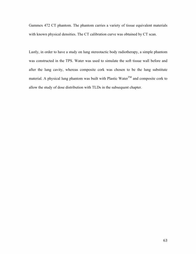
  63  

Gammex 472 CT phantom. The phantom carries a variety of tissue equivalent materials

with known physical densities. The CT calibration curve was obtained by CT scan.

Lastly, in order to have a study on lung stereotactic body radiotherapy, a simple phantom

was constructed in the TPS. Water was used to simulate the soft tissue wall before and

after the lung cavity, whereas composite cork was chosen to be the lung substitute

material. A physical lung phantom was built with Plastic WaterTM and composite cork to

allow the study of dose distribution with TLDs in the subsequent chapter.

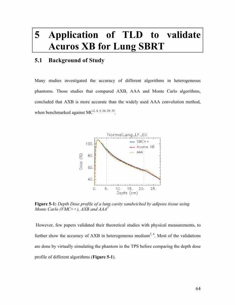
  64  

5 Application of TLD to validate Acuros XB for Lung SBRT

5.1 Background of Study

Many studies investigated the accuracy of different algorithms in heterogeneous

phantoms. Those studies that compared AXB, AAA and Monte Carlo algorithms,

concluded that AXB is more accurate than the widely used AAA convolution method,

when benchmarked against MC2, 4, 5, 24, 29, 35.

Figure 5-1: Depth Dose profile of a lung cavity sandwiched by adipose tissue using Monte Carlo (VMC++), AXB and AAA3

However, few papers validated their theoretical studies with physical measurements, to

further show the accuracy of AXB in heterogeneous medium2, 4. Most of the validations

are done by virtually simulating the phantom in the TPS before comparing the depth dose

profile of different algorithms (Figure 5-1).

Figure 3 EGSnrc and VMC++ comparison. Depth dose curves (DD) at -4 cm off-axis for the SF, 6X case in Normal Lung, Light Lung and Bonefor EGSnrc and VMC++.

Figure 4 Depth dose curves (DD) at -4 cm off-axis. Dose to medium calculations for VMC++, Acuros XB version 10, and AAA in phantom A. Incolumns: Normal Lung, Light Lung, Bone; in rows: SF and LF for 6X, SF and LF for 15X.

Fogliata et al. Radiation Oncology 2011, 6:82http://www.ro-journal.com/content/6/1/82

Page 7 of 15

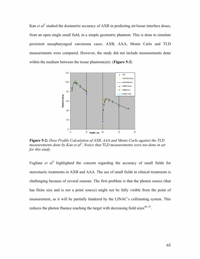
  65  

Kan et al2 studied the dosimetric accuracy of AXB in predicting air/tissue interface doses,

from an open single small field, in a simple geometric phantom. This is done to simulate

persistent nasopharyngeal carcinoma cases. AXB, AAA, Monte Carlo and TLD

measurements were compared. However, the study did not include measurements done

within the medium between the tissue phantom(air). (Figure 5-2)

Figure 5-2: Dose Profile Calculation of AXB, AAA and Monte Carlo against the TLD measurements done by Kan et al2. Notice that TLD measurements were not done in air for this study.

Fogliata et al5 highlighted the concern regarding the accuracy of small fields for

stereotactic treatments in AXB and AAA. The use of small fields in clinical treatments is

challenging because of several reasons. The first problem is that the photon source (that

has finite size and is not a point source) might not be fully visible from the point of

measurement, as it will be partially hindered by the LINAC’s collimating system. This

reduces the photon fluence reaching the target with decreasing field sizes46, 47.

4709 Kan, Leung, and Yu: Impact of Acuros XB on IMSRT for NPC 4709

infrared optical system. IMSRT planning was performed withthe Eclipse planning system using sliding window technique.

The final dose calculations of the original patient planswere performed by AAA with inhomogeneity correction us-ing 1.0 mm grid resolution. AXB dose calculation using 1.0mm grid resolution of each plan was performed retrospec-tively using exactly the same monitor units and MLC leafmovement setting as the corresponding AAA plan. Dose–volume histograms (DVHs) were produced for all plans sothat the doses to the PTV and OARs could be analyzed. Forthe PTV, the maximum dose, minimum dose, the coveragerepresented by V>95% (the volume receiving more than 95%of the reference dose), V>100% and the hot areas representedby V>110% were reported and compared between the predic-tion from the two algorithms. For the OARs, the dose encom-passing 1% (D1%) and 5% (D5%) of the volumes for brainstem, spinal cord, optic chiasm, optic nerve, and the meandoses to lens were also reported and compared. The plan con-formity was evaluated through comparisons using the con-formation number, CN, which was defined as the product ofVT,ref/VT and VT,ref/Vref, where VT,ref represents the volumeof the target receiving a dose equal to or greater than the ref-erence dose; VT represents the physical volume of the target,and Vref represents the total tissue volume receiving a doseequal to or greater than the reference dose.15 The referencedose used to compute the CN is the prescription dose. Thefirst ratio assesses quality of target coverage, and the secondratio assesses the amount of healthy tissue being involved inthe reference dose. The higher the CN values, the better theconformity. A CN value of 1 represents perfect conformity.

III. RESULTS

III.A. Verification of PDD in the rectangular phantomwith air cavity

It is seen from Figs. 3(a) to 3(c) that the Monte Carlo sim-ulated PDD data matched quite closely to the TLD measuredPDD. The results from the calculations using AAA are in-adequate to predict accurately the secondary build-up at andalso the first 1 cm beyond the distal interface between air andsolid water from 2 ! 2 to 5 ! 5 cm2 fields. If taking the mea-sured data by TLD as the reference (the accuracy of the TLDmeasurement was about 3%), the PDD measured at the dis-tal air/solid water interface was 16.3%, 23.3%, and 38.2% forthe 2 ! 2, 3 ! 3, and 5 ! 5 cm2 field, respectively, whilethose predicted by AAA using 1.0 mm grid size (AAA1.0 mm)were 57.1%, 60.0%, and 64.0%, respectively. The overesti-mation of PDD at the distal interface by AAA1.0 mm was upto 41% when 2 ! 2 cm2 field was used. On the other hand,significant improvement in predicting the secondary build-upcurves by AXB was observed. Overestimations of PDD byAXB were still observed at the distal air/solid water inter-face. The predicted PDD was 22.5%, 26.7%, and 45.5%, re-spectively, when using 1.0 mm grid size. The distal interfacePDD was overestimated by about 6% for 2 ! 2 cm2 by AXBusing 1.0 mm grid size (AXB1.0 mm). However, at depths 2mm or more beyond the distal interface, the predicted PDD

FIG. 3. The predicted percentage depth dose curves predicted by AAA andAXB compared to the measured and Monte Carlo simulated data using therectangular phantom for (a) 2 ! 2 cm2, (b) 3 ! 3 cm2, and (c) 5 ! 5 cm2

fields. The measured data and Monte Carlo simulated data were from Kanet al. (Ref. 7).

Medical Physics, Vol. 39, No. 8, August 2012

  66  

The second problem is that the fields might be small when compared to the maximum

lateral range of secondary electrons. This will result in a high dependence of the

computed and delivered dose on the density of the irradiated media48, 49.

Lastly, according to Bragg-Gray Cavity theory15, 50, an ideal dosimeter must be small

when compared to the field size of the beam, so that the dosimeter will not perturb the

fluence of the particles in the medium. However, at small fields, such ideal dosimeters

does not exist51.

Hence, in this study, the motivation is to validate the accuracy of AXB for Lung

Stereotactic Body Radiotherapy, in small, medium and standard field sizes, using TLDs.

This study will also check the results obtained against the AAA convolution method as

done in previous studies2, 4, 5, 24, 29, 35. The lung dose is of particular interest because it

relates to complications arising from high dose treatment to the tumor52.

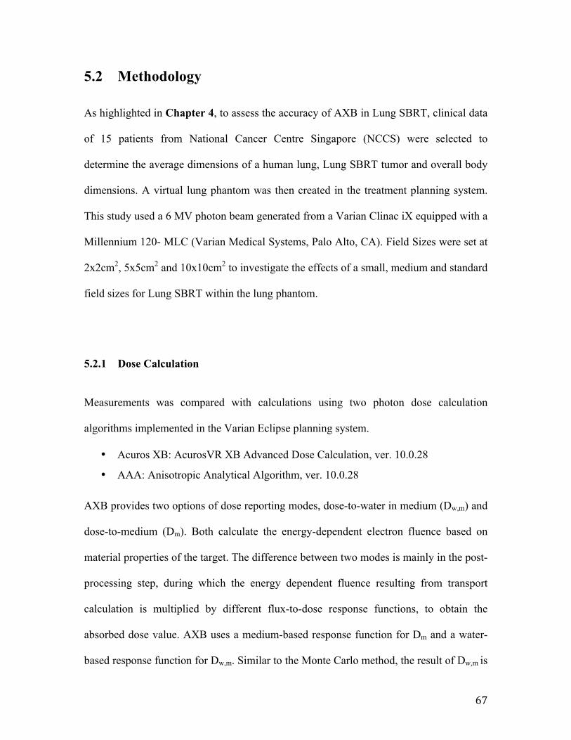
  67  

5.2 Methodology  As highlighted in Chapter 4, to assess the accuracy of AXB in Lung SBRT, clinical data

of 15 patients from National Cancer Centre Singapore (NCCS) were selected to

determine the average dimensions of a human lung, Lung SBRT tumor and overall body

dimensions. A virtual lung phantom was then created in the treatment planning system.

This study used a 6 MV photon beam generated from a Varian Clinac iX equipped with a

Millennium 120- MLC (Varian Medical Systems, Palo Alto, CA). Field Sizes were set at

2x2cm2, 5x5cm2 and 10x10cm2 to investigate the effects of a small, medium and standard

field sizes for Lung SBRT within the lung phantom.

5.2.1 Dose Calculation

 Measurements was compared with calculations using two photon dose calculation

algorithms implemented in the Varian Eclipse planning system.

• Acuros XB: AcurosVR XB Advanced Dose Calculation, ver. 10.0.28

• AAA: Anisotropic Analytical Algorithm, ver. 10.0.28

AXB provides two options of dose reporting modes, dose-to-water in medium (Dw,m) and

dose-to-medium (Dm). Both calculate the energy-dependent electron fluence based on

material properties of the target. The difference between two modes is mainly in the post-

processing step, during which the energy dependent fluence resulting from transport

calculation is multiplied by different flux-to-dose response functions, to obtain the

absorbed dose value. AXB uses a medium-based response function for Dm and a water-

based response function for Dw,m. Similar to the Monte Carlo method, the result of Dw,m is

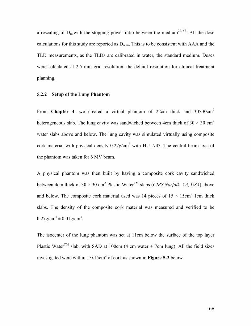
  68  

a rescaling of Dm with the stopping power ratio between the medium22, 53. All the dose

calculations for this study are reported as Dw,m. This is to be consistent with AAA and the

TLD measurements, as the TLDs are calibrated in water, the standard medium. Doses

were calculated at 2.5 mm grid resolution, the default resolution for clinical treatment

planning.

5.2.2 Setup of the Lung Phantom

 From Chapter 4, we created a virtual phantom of 22cm thick and 30×30cm2

heterogeneous slab. The lung cavity was sandwiched between 4cm thick of 30 × 30 cm2

water slabs above and below. The lung cavity was simulated virtually using composite

cork material with physical density 0.27g/cm3 with HU -743. The central beam axis of

the phantom was taken for 6 MV beam.

A physical phantom was then built by having a composite cork cavity sandwiched

between 4cm thick of 30 × 30 cm2 Plastic WaterTM slabs (CIRS Norfolk, VA, USA) above

and below. The composite cork material used was 14 pieces of 15 × 15cm2 1cm thick

slabs. The density of the composite cork material was measured and verified to be

0.27g/cm3 ± 0.01g/cm3.

The isocenter of the lung phantom was set at 11cm below the surface of the top layer

Plastic WaterTM slab, with SAD at 100cm (4 cm water + 7cm lung). All the field sizes

investigated were within 15x15cm2 of cork as shown in Figure 5-3 below.

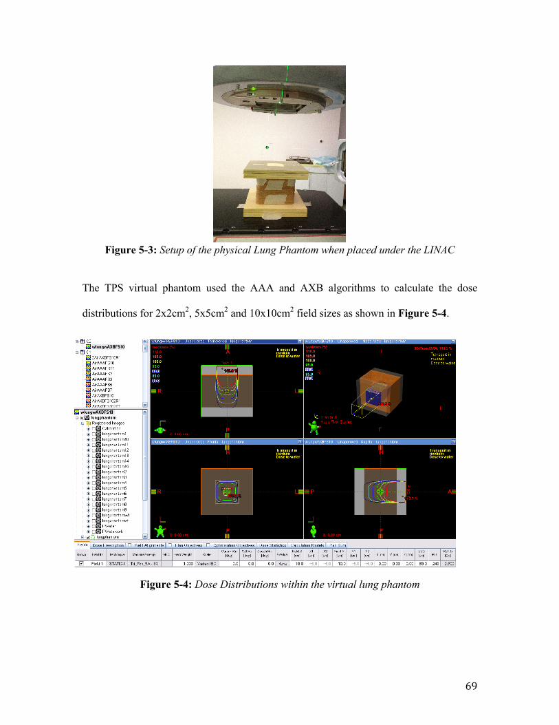
  69  

Figure 5-3: Setup of the physical Lung Phantom when placed under the LINAC

The TPS virtual phantom used the AAA and AXB algorithms to calculate the dose

distributions for 2x2cm2, 5x5cm2 and 10x10cm2 field sizes as shown in Figure 5-4.

Figure 5-4: Dose Distributions within the virtual lung phantom

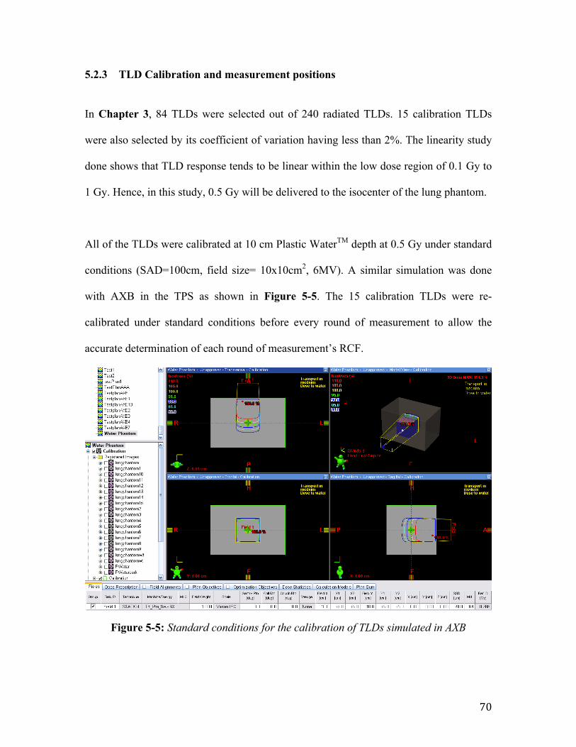
  70  

5.2.3 TLD Calibration and measurement positions

 In Chapter 3, 84 TLDs were selected out of 240 radiated TLDs. 15 calibration TLDs

were also selected by its coefficient of variation having less than 2%. The linearity study

done shows that TLD response tends to be linear within the low dose region of 0.1 Gy to

1 Gy. Hence, in this study, 0.5 Gy will be delivered to the isocenter of the lung phantom.

All of the TLDs were calibrated at 10 cm Plastic WaterTM depth at 0.5 Gy under standard

conditions (SAD=100cm, field size= 10x10cm2, 6MV). A similar simulation was done

with AXB in the TPS as shown in Figure 5-5. The 15 calibration TLDs were re-

calibrated under standard conditions before every round of measurement to allow the

accurate determination of each round of measurement’s RCF.

Figure 5-5: Standard conditions for the calibration of TLDs simulated in AXB  

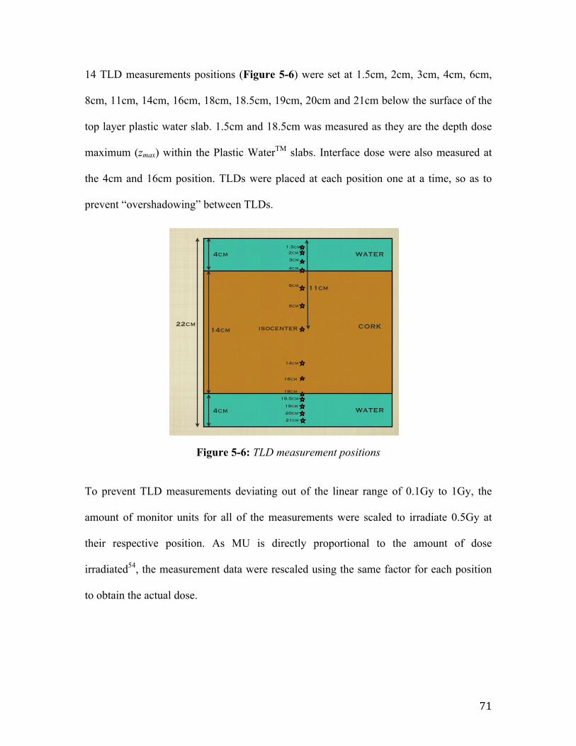
  71  

14 TLD measurements positions (Figure 5-6) were set at 1.5cm, 2cm, 3cm, 4cm, 6cm,

8cm, 11cm, 14cm, 16cm, 18cm, 18.5cm, 19cm, 20cm and 21cm below the surface of the

top layer plastic water slab. 1.5cm and 18.5cm was measured as they are the depth dose

maximum (zmax) within the Plastic WaterTM slabs. Interface dose were also measured at

the 4cm and 16cm position. TLDs were placed at each position one at a time, so as to

prevent “overshadowing” between TLDs.

Figure 5-6: TLD measurement positions

To prevent TLD measurements deviating out of the linear range of 0.1Gy to 1Gy, the

amount of monitor units for all of the measurements were scaled to irradiate 0.5Gy at

their respective position. As MU is directly proportional to the amount of dose

irradiated54, the measurement data were rescaled using the same factor for each position

to obtain the actual dose.

Isocenter set at 11cm below Surface

lung - 14cm Water - 4cm

PDD measurement:2cm before interfaceat interface2cm after interfaceIsocenter

0.01cm3 water volume of density 2.64g/cm3 as simulated TLD

MEASUREMENTS

22cm

4cm

4cm

14cm

11cm

isocenter

1.5cm

WATER

WATER

CORK

2cm

3cm

4cm

6cm

8cm

14cm

16cm

18cm

18.5cm

19cm

20cm

21cm

Wednesday, March 13, 13

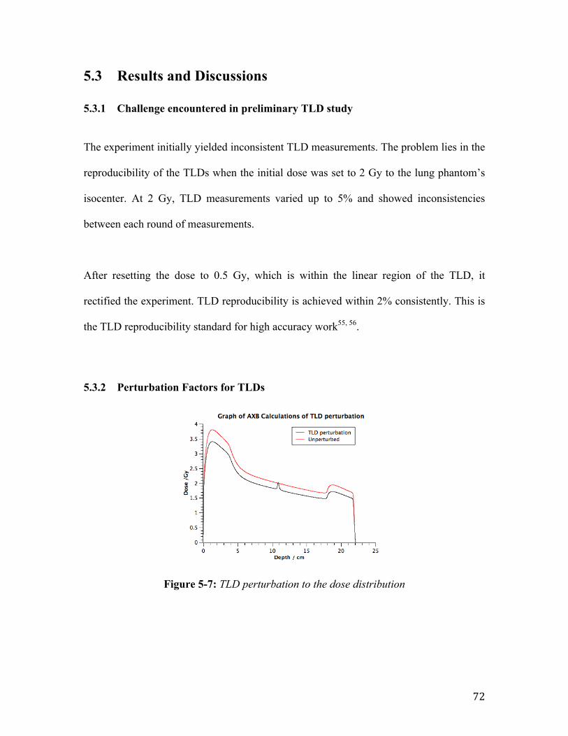
  72  

5.3 Results and Discussions

5.3.1 Challenge encountered in preliminary TLD study

 The experiment initially yielded inconsistent TLD measurements. The problem lies in the

reproducibility of the TLDs when the initial dose was set to 2 Gy to the lung phantom’s

isocenter. At 2 Gy, TLD measurements varied up to 5% and showed inconsistencies

between each round of measurements.

After resetting the dose to 0.5 Gy, which is within the linear region of the TLD, it

rectified the experiment. TLD reproducibility is achieved within 2% consistently. This is

the TLD reproducibility standard for high accuracy work55, 56.

5.3.2 Perturbation Factors for TLDs

Figure 5-7: TLD perturbation to the dose distribution

factor[9] and reader calibration factor (RCF).[11,12] Following da Rosa et al. [9] who used Monte Carlo simulation, the TLD perturbation factors in lung were calculated with AXB by inserting a small water volume of 0.01cm3 drawn in the dimension of the TLD and positioned in composite cork. The density of the water volume was taken to be 2.64 g/cm3, which is the density of TLD-100. The TLD-100 is assumed to be radiological water equivalent as its effective atomic number (8.14) is sufficiently close to biological tissues.[13] The grid resolution used was 1.0 mm given the small volume. The corrected TLD doses were then compared with the predicted dose by AXB and AAA. All dose calculations were performed to deliver 2 Gy to the isocenter.

III. RESULTS

A. Perturbation factor caused by TLD in lung (AXB)

Fig.3: TLD PDD perturbation in AXB

Table 1 Perturbation Factors from AXB

Material Depth/cm Perturbation factor

Plastic Water 2 None

Plastic Water 4 None

Composite Cork 6 1.077

Composite Cork 11 1.102

Composite Cork 16 1.084

Composite Cork 18 1.086

Plastic Water 20 None

It was found that the AXB predicted perturbation factor was 1.102 at isocentre as shown in Fig.3. This perturbation factor was calculated by the shift in PDD predicted in AXB. In order to calculate the factor in the other positions within composite cork, the normalization point was fixed at isocentre and the difference in the peak reading and the unperturbed PDD was calculated. Results are shown in Table 1. Perturbations within composite cork ranges from 1.077-1.102.

B. Verification of PDD in the lung substitute phantom

Fig.4: TLD PDD comparison of 2×2cm2 field size

It is seen from Fig.4 that the AXB data matches closely to the TLD measured PDD to within an average of 2.2%. The results from the calculations using AAA are generally good (to within 2.4%) but the greatest deviation is 7% (as compared to 2.5% in AXB) occured at 2cm after the water/cork interface. Uncertainties associated with the TLD measurement was estimated at 5%, which is due largely to the repeatability of the measured dose per cycle relative to dose measured in first cycle.[14]

IV. DISSCUSSIONS

Some previous investigations showed that AXB was capable of accounting for specific material composition of the media, which would result in improved accuracy of dose calculation in heterogeneous media, as compared to the commonly used AAA.[3,15] The TLD verification of AXB using a lung substitute material is an important step to determine the reliability of AXB for small field Lung SBRT. However, TLD-100, with its finite dimensions and relatively higher density, causes significant perturbation in a low-density lung medium. This has to be accounted for. AXB proved to be self consistent as shown in the accuracy of the corrected TLD readings. Final results from the lung

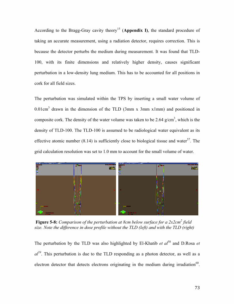
  73  

According to the Bragg-Gray cavity theory15 (Appendix I), the standard procedure of

taking an accurate measurement, using a radiation detector, requires correction. This is

because the detector perturbs the medium during measurement. It was found that TLD-

100, with its finite dimensions and relatively higher density, causes significant

perturbation in a low-density lung medium. This has to be accounted for all positions in

cork for all field sizes.

The perturbation was simulated within the TPS by inserting a small water volume of

0.01cm3 drawn in the dimension of the TLD (3mm x 3mm x1mm) and positioned in

composite cork. The density of the water volume was taken to be 2.64 g/cm3, which is the

density of TLD-100. The TLD-100 is assumed to be radiological water equivalent as its

effective atomic number (8.14) is sufficiently close to biological tissue and water57. The

grid calculation resolution was set to 1.0 mm to account for the small volume of water.

Figure 5-8: Comparison of the perturbation at 8cm below surface for a 2x2cm2 field size. Note the difference in dose profile without the TLD (left) and with the TLD (right)

The perturbation by the TLD was also highlighted by El-Khatib et al58 and D.Rosa et

al59. This perturbation is due to the TLD responding as a photon detector, as well as a

electron detector that detects electrons originating in the medium during irradiation60.

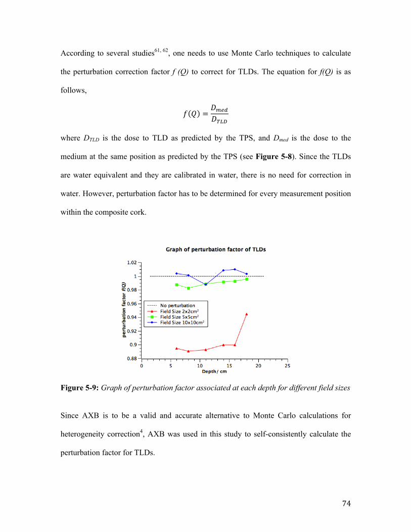
  74  

According to several studies61, 62, one needs to use Monte Carlo techniques to calculate

the perturbation correction factor f (Q) to correct for TLDs. The equation for f(Q) is as

follows,

𝑓 𝑄 =𝐷!"#𝐷!"#

where DTLD is the dose to TLD as predicted by the TPS, and Dmed is the dose to the

medium at the same position as predicted by the TPS (see Figure 5-8). Since the TLDs

are water equivalent and they are calibrated in water, there is no need for correction in

water. However, perturbation factor has to be determined for every measurement position

within the composite cork.

Figure 5-9: Graph of perturbation factor associated at each depth for different field sizes

Since AXB is to be a valid and accurate alternative to Monte Carlo calculations for

heterogeneity correction4, AXB was used in this study to self-consistently calculate the

perturbation factor for TLDs.

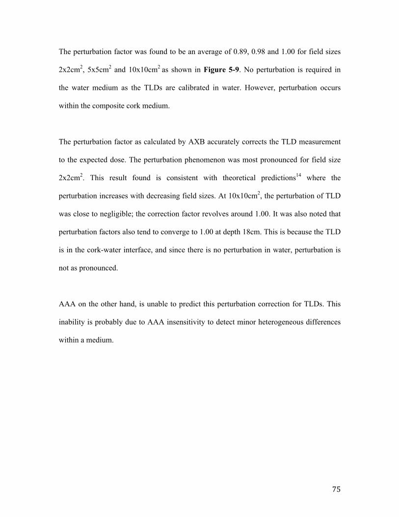
  75  

The perturbation factor was found to be an average of 0.89, 0.98 and 1.00 for field sizes

2x2cm2, 5x5cm2 and 10x10cm2 as shown in Figure 5-9. No perturbation is required in

the water medium as the TLDs are calibrated in water. However, perturbation occurs

within the composite cork medium.

The perturbation factor as calculated by AXB accurately corrects the TLD measurement

to the expected dose. The perturbation phenomenon was most pronounced for field size

2x2cm2. This result found is consistent with theoretical predictions14 where the

perturbation increases with decreasing field sizes. At 10x10cm2, the perturbation of TLD

was close to negligible; the correction factor revolves around 1.00. It was also noted that

perturbation factors also tend to converge to 1.00 at depth 18cm. This is because the TLD

is in the cork-water interface, and since there is no perturbation in water, perturbation is

not as pronounced.

AAA on the other hand, is unable to predict this perturbation correction for TLDs. This

inability is probably due to AAA insensitivity to detect minor heterogeneous differences

within a medium.

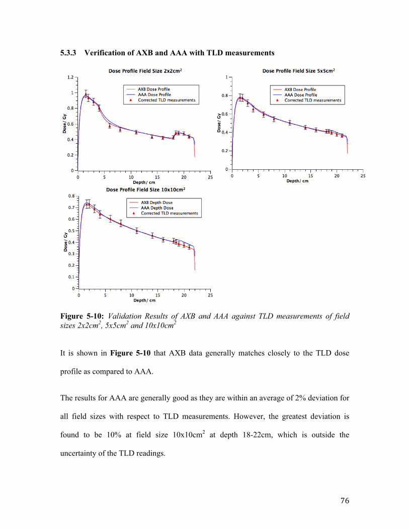
  76  

5.3.3 Verification of AXB and AAA with TLD measurements

 

Figure 5-10: Validation Results of AXB and AAA against TLD measurements of field sizes 2x2cm2, 5x5cm2 and 10x10cm2

It is shown in Figure 5-10 that AXB data generally matches closely to the TLD dose

profile as compared to AAA.

The results for AAA are generally good as they are within an average of 2% deviation for

all field sizes with respect to TLD measurements. However, the greatest deviation is

found to be 10% at field size 10x10cm2 at depth 18-22cm, which is outside the

uncertainty of the TLD readings.

  77  

AXB dose in lung phantom is better than AAA as its deviation have an average of 1% for

all field sizes with respect to the TLD measurements. Its greatest deviation is 5% at field

size 2x2cm2 at depth 8cm, but it is still within the uncertainty of TLD measurement. This

result found is consistent with theoretical validation of AXB with Monte Carlo

simulations1, 4, 30.

Uncertainties associated with the TLD measurement was estimated at 5%. Besides the

reproducibility of ±2%3, 63, factors that affect this uncertainty are errors associated when

determining the perturbation factor of the TLD, variation of TLD density, variation in

density of different slices of composite cork, and the placement of TLDs on the planchet

in the TLD reader during readout. An estimation of overall 5% uncertainty is therefore

reported in this study. This will be discussed further in the next section.

5.3.4 Discussions

 Some previous investigations showed that AXB, accounting for specific material

composition of the medium, have improved accuracy of dose calculation in

heterogeneous media, as compared to the widely used AAA3, 30. The TLD verification of

AXB is an important step to determine the reliability of AXB for small field Lung SBRT.

Since AXB is a simulation of the dose distribution, it must be benchmarked against the

physical dose measurement of a radiation dosimeter.

The TLD dosimetric system has been calibrated for high precision measurements as far

as possible to be the benchmark for this validation. However, TLD-100, with its finite

  78  

dimensions and relatively higher density, causes significant perturbation in a low-density

lung medium, which is especially so in small fields. The determination of the

perturbation factors may incur some errors to the TLD measurements.

Table 5-1: Percentage error in calculating TLD perturbation factor  

Density g/cc

% diff density

Perturbation Factor % error

2.638 0% 0.901 0.004 2.506 95% 0.904 -0.6 2.374 90% 0.910 -0.05 2.771 105% 0.897 -1.39 2.903 110% 0.894 -1.77

TLDs may differ in density from one another due to manufacturing fault as there is ±15%

sample-to-sample uniformity as reported by Radiation Products Design, Inc64. By

assuming that TLDs may have a 10% density variation from its default density

2.64g/cm3, there may be a percentage error of the perturbation factor up to 1.7% as

shown in Table 1 above.

The composite cork chosen may also differ in density between slices. Even though that

15 slices of composite cork have an average density of 0.27g/cm3, density of each

individual slices calculated may vary up to 3%. The density was calculated by measuring

the mass and volume of each slice of composite cork individually.

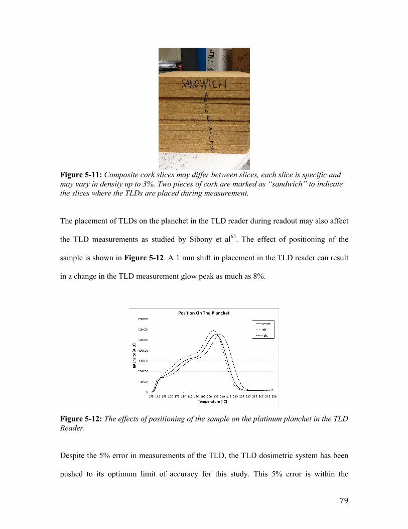
  79  

Figure 5-11: Composite cork slices may differ between slices, each slice is specific and may vary in density up to 3%. Two pieces of cork are marked as “sandwich” to indicate the slices where the TLDs are placed during measurement.

The placement of TLDs on the planchet in the TLD reader during readout may also affect

the TLD measurements as studied by Sibony et al65. The effect of positioning of the

sample is shown in Figure 5-12. A 1 mm shift in placement in the TLD reader can result

in a change in the TLD measurement glow peak as much as 8%.

Figure 5-12: The effects of positioning of the sample on the platinum planchet in the TLD Reader.

Despite the 5% error in measurements of the TLD, the TLD dosimetric system has been

pushed to its optimum limit of accuracy for this study. This 5% error is within the

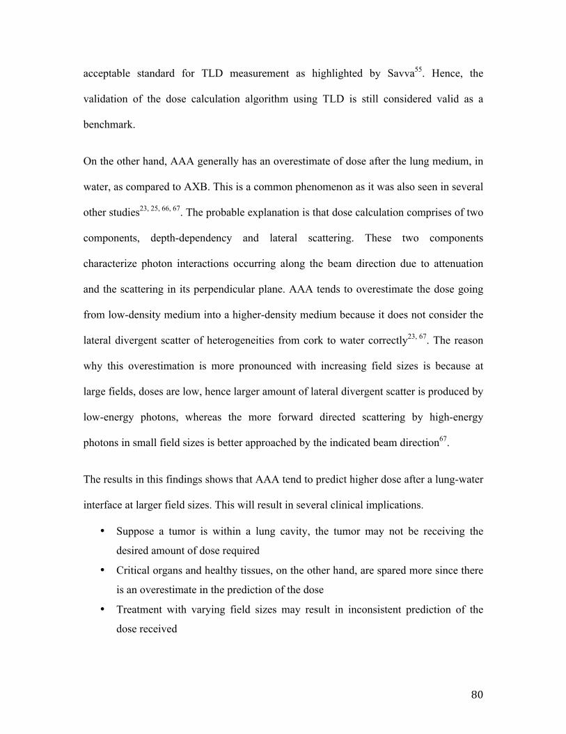
  80  

acceptable standard for TLD measurement as highlighted by Savva55. Hence, the

validation of the dose calculation algorithm using TLD is still considered valid as a

benchmark.

On the other hand, AAA generally has an overestimate of dose after the lung medium, in

water, as compared to AXB. This is a common phenomenon as it was also seen in several

other studies23, 25, 66, 67. The probable explanation is that dose calculation comprises of two

components, depth-dependency and lateral scattering. These two components

characterize photon interactions occurring along the beam direction due to attenuation

and the scattering in its perpendicular plane. AAA tends to overestimate the dose going

from low-density medium into a higher-density medium because it does not consider the

lateral divergent scatter of heterogeneities from cork to water correctly23, 67. The reason

why this overestimation is more pronounced with increasing field sizes is because at

large fields, doses are low, hence larger amount of lateral divergent scatter is produced by

low-energy photons, whereas the more forward directed scattering by high-energy

photons in small field sizes is better approached by the indicated beam direction67.

The results in this findings shows that AAA tend to predict higher dose after a lung-water

interface at larger field sizes. This will result in several clinical implications.

• Suppose a tumor is within a lung cavity, the tumor may not be receiving the

desired amount of dose required

• Critical organs and healthy tissues, on the other hand, are spared more since there

is an overestimate in the prediction of the dose

• Treatment with varying field sizes may result in inconsistent prediction of the

dose received

  81  

However, Lung SBRT cases are delivered with multiple beams from many directions

(Figure 4-5). This may cause the dose differences to be averaged out when using

conventional AAA algorithm. This is a subject of further study.

AXB has proven to be accurate and self-consistent as shown in our TLD measurements.

Final results from the lung substitute phantom shows that AXB’s accuracy under

electronic disequilibrium condition for small field size (2x2cm2) is better than AAA. This

validates the theory that AXB is an accurate dose algorithm as reported in several

studies3, 28. It should be considered for clinical application for Lung SBRT.

  82  

5.4 Summary

In this chapter, AXB was validated for Lung SBRT using TLD-100 and checked against

AAA, in a lung substitute phantom. The motivation for this study was that many papers

have validated AXB by simulating the dose in the TPS without physical measurements.

The lung phantom was built by having a slab of 14cm composite cork sandwiched by

4cm slabs of Plastic Water. The dimensions of the phantom were obtained by taking the

average dimensions of 15 Lung SBRT patients treated in National Cancer Center

Singapore. Composite cork was chosen as a lung substitute material, as it was found to

have similar radiological properties as lung tissue.

TLDs were calibrated at 0.5Gy under standard condition in 10cm Plastic Water. 0.5Gy

was then delivered to lung isocenter as it was found to be within the linear range of the

TLD response. 14 TLD measurement positions were placed within the lung phantom,

including the water-cork (lung) interfaces and the lung isocenter.

It was found that TLD-100, with its finite dimensions and relatively higher density,

causes significant perturbation in a low-density lung medium. This has to be accounted

for each of the field sizes. AXB was used to calculate the perturbation factor for TLDs in

this study. As field sizes decreases, the perturbation of the TLD increases. The AXB

perturbation factors also validates its accuracy to correct the TLD readings and hence its

self-consistency.

  83  

AXB data generally matches closely to the TLD dose profile as compared to AAA. The

perturbation factor as calculated by AXB accurately corrects for the TLD measurement

back to the expected dose. Uncertainties associated with the TLD measurement was

estimated at 5%. These errors include the ±2% reproducibility, the variation of density in

TLDs, variation in density of different slices of composite cork, and also the placement of

TLDs on the planchet in the TLD reader during readout.

AAA generally has an overestimate of dose after lung medium in water and this becomes

more pronounced with increasing field sizes. This is due to divergent scatter between

heterogeneous interfaces that is not accounted for in the AAA model.

TLD measurements have shown that the AXB results are more accurate than AAA in

lung. Results obtained imply that AXB should be considered for clinical application in

Lung SBRT treatment.

  84  

6 Conclusion 6.1 Summary

The end goal of physics in radiotherapy is to treat a target volume with the appropriate

amount of dose and yet minimizing dose to healthy tissues and critical organs. A brief

introduction of the physics of radiotherapy was done in Chapter 2, to help readers

understand some key concepts pertaining to radiation physics.

 The objective of this work is to study thermoluminesence dosimeters and apply them to

validate a new the dose calculation algorithm, Acuros XB. This validation of the dose

calculation algorithm was done for Lung Stereotactic Body Radiation Therapy cases. The

result in this study will have clinical implications on the use of the appropriate algorithms

for Lung SBRT cases.

In Chapter 3, a study was done on thermoluminence dosimetry. Through the calibration

and selection of TLDs, we determined several correction factors such as Reader

Correction Factor and Element Correction Coefficient. These are essential to obtain an

accurate measurement using TLDs. The linearity response of the TLDs was also

investigated.

Dose calculation algorithms were introduced in Chapter 4. Two dose calculation

algorithms, Anistropic Analytical Algorithm and Acuros XB, was studied. AAA is a

clinical algorithm that is widely used today. AXB is a new dose calculation algorithm,

  85  

and was reported that it has excellent agreement with the gold standard for dose

calculation today, which is Monte Carlo calculation. AXB depends on the CT number –

mass density relationship to account for heterogeneities within a medium. A CT

calibration curve was obtained by having a CT scan of 2 different electron density

phantoms.

A lung phantom was built to simulate Lung SBRT cases. In earlier studies, composite

cork was found to be the best lung substitute material. Plastic WaterTM was used to

simulate soft tissue wall before and after the lung cavity.

Lastly, we validated AXB and AAA by taking 14 TLD measurements within the lung

phantom in Chapter 5. It was found that the high-density TLD cause significant

perturbation within the low-density lung medium. Hence, the TLD measurements have to

be corrected by a perturbation factor calculated using AXB. AAA, on the other hand, is

unable to determine this factor due to limitations in the algorithm.

It was found that AXB agrees with TLD measurements better than AAA. AAA tends to

have an overestimation in water after the low-density lung medium, and this phenomenon

was more pronounced with increasing field sizes. This is due to lateral divergent

scattering at low photon doses at large field sizes, as compared to forward directed

scattering in high photon doses at small field sizes. By such an overestimation, there will

be clinical implications when using AAA for Lung SBRT. For example, a tumor may not

be receiving the desired dose as there is an overestimation using AAA. However,

  86  

conventional Lung SBRT is delivered with multiple beams from many directions. This

might have caused the dose differences to be averaged out, self- correcting it to the

desired dose. Further studies could be done to investigate this implication.

 

  87  

6.2 Future Works

In this study, AAA overestimated the doses after the low-density lung medium at large

field sizes. However, this prediction was after a 14cm lung cavity. Most Lung SBRT

cases have a tumor at intermediate depths, such as after 5cm of lung cavity. Investigation

can be done to study the overestimation of AAA in a small tumor inserted at a mid-lung

position.

Most Lung SBRT cases are done using 4D-CT scans. Conventional CT scans simulate

the patient’s lung volume by compiling several image slices of the lung volume.

However, due to the respiratory motion of the patient, it is impossible to determine the

position of the tumor. A 4D-CT scan comprises of a large number of individual CT scans

obtained at various phases of the respiratory cycle68. This approach images the movement

of the tumor with respiration and it helps to determine an accurate internal margin for the

tumor. Hence, future works could create a lung phantom that is able to simulate the

respiratory movement of a patient. Further validation of AXB and AAA could be done

using TLDs on 4D-CT Lung SBRT.

A new version of AXB (ver. 11) will also be ready in the future. A comparison of AXB

and AAA from version 11 with AXB and AAA from version 10 can be done to

investigate the improvements in lung cases.

  88  

7 References  1.   T.  Han,  F.  Mourtada,  K.  Kisling,  J.  Mikell,  D.  Followill  and  R.  Howell,  Med.  Phys.  

38,  2651–2664  (2011).  2.   M.  W.  K.  Kan,  L.  H.  T.  Leung  and  P.  K.  N.  Yu,  Med.  Phys.  39  (8)  (August  2012).  3.   A.  Fogliata,  G.  Nicolini,  A.  Clivio,  E.  Vanetti  and  L.  Cozzi,  Radiation  Oncology  6  

(82)  (2011).  4.   A.   Fogliata,   G.   Nicolini,   A.   Clivio,   E.   Vanetti,   P.   Mancosu   and   L.   Cozzi,   Phys.  

Med.  Biol.  56,  1879-­‐1904  (2011).  5.   A.  Fogliata,  G.  Nicolini,  A.  Clivio,  E.  Vanetti  and  L.  Cozzi,  Am.  Assoc.  Phys.  Med.  

38  (11)  (2011).  6.   Tao  Han,  Firas  Mourtada,  Kelly  Kisling,  Justin  Mikell,  David  Followill,  Rebecca  

Howell,  Med.  Phys.  39  (4)  (2012).  7.   K.-­‐P.  Chang,  S.-­‐H.  Hung,  Y.-­‐H.  Chie,  A.-­‐C.  Shiau  and  R.-­‐J.  Huang,  Med.  Phys.  39  

(4)  (2012).  8.   M.  Goitein,  Radiation  Oncology:  A  Physicist's-­‐Eye  View.  (Springer,  2008).  9.   E.   B.   Podgorsak,   Radiation   Oncology   Physics:   A   Handbook   for   Teachers   and  

Students.  (IAEA,  2005).  10.   Paul   N.   Mobit   ,   Great   Lakes   Cancer   Institute   ,McLaren   Regional   Medical  

Center   and   Tomas   Kron,   Peter   MacCallum   Cancer   Centre,   Department   of  Physical   Sciences,   in   MICRODOSIMETRIC   RESPONSE   OF   PHYSICAL   AND  BIOLOGICAL   SYSTEMS   TO   LOW-­‐   AND  HIGH-­‐LET   RADIATIONS:   THEORY   AND  APPLICATIONS  TO  DOSIMETRY,  edited  by  Y.  Horowitz  (Elsevier  B.V,  2006).  

11.   F.  Daniels,  Boyd,  C.  and  Saunders,  Science  117,  343–349  (1953).  12.   J.   V.   Dam   and   G.   Marinello,   in   ESTRO   (ESTRO,   Mounierlaan   83/12   –   1200  

Brussels  (Belgium),  2006).  13.   McKinlay,   Thermoluminescence   dosimetry-­‐Medical   Physics   Handbooks   5.  

(Bristol:  Adam  Hilger  Ltd,  1981).  14.   P.  N.  Mobit,  A.  E.  Nahum,  Philip  Mayles,  Joint  Department  of  Physics,  Institute  

of  Cancer  Research  and  Royal  Marsden  NHS  Trust,   and  U.   Sutton  SM2  5PT,  Phys.  Med.  Biol.  41,  979-­‐993  (1996).  

15.   P.  N.  Mobit,  P.  Mayles,  Alan  E  Nahum,  Joint  Department  of  Physics,  Institute  of  Cancer  Research  and  Royal  Marsden  NHS  Trust,  Sutton  and  U.  SM2  5PT,  Phys.  Med.  Biol.  41,  387-­‐398  (1996).  

16.   T.  Kron,  Australas.  Phys.  Eng.  Sci.  Med.  18,  1-­‐25  (1994).  17.   Saint-­‐Gobain   Industrial   Ceramics,   Inc.,   Harshaw   Dosimetry   System,   (TLD  

Reader,   REMS,   and   Dose   Computation   Algorithm),   System   Calibration  Procedure,  USA  (1998).  

18.   D.  M.  Moor,  B.  Horspool  and  R.  P.  Stokes,  Radiation  Measurements  43,  533–537  (2008).  

19.   International  Commission  on  Radiological  Protection.  Radiological  Protection  and  Safety  in  Medicine,  ICRP  Publication  73  (Annals  of  ICRP  26  (2).)  (1996).  

20.   T.  Rivera,  Applied  Radiation  and  Isotopes  10,  1016  (2012).  

  89  

21.   Y.   S.   Horowitz   and   H.   Datz,   presented   at   the   American   Institute   of   Physics  conference  Proceedings,  2011  (unpublished).  

22.   L.  A.  R.  d.  Rosa,  S.  C.  Cardoso,  L.  T.  Campos,  V.  G.  L.  Alves,  D.  V.  S.  Batista  and  A.  .Facure,  Journal  Of  Applied  Clinical  Medical  Physics  11  (1)  (2010).  

23.   E.   Sterpin,   M.   Tomsej,   B.   De   Smedt,   N.   Reynaert   and   S.   Vynckier,   Medical  Physics  34,  1665  (2007).  

 24.   A.  Fogliata,  G.  Nicolini,  E.  Vanetti,  A.  Clivio  and  L.  Cozzi,  Physics   in  Medicine  and  Biology,  51,  1421–1438  (2006).  

25.   C.   M.   Bragg   and   J.   Conway,   Radiotherapy   and   Oncology   81   (3),   315-­‐323  (2006).  

26.   K.   Breitman,   S.   Rathee,   C.   Newcomb,   B.   Murray,   D.   Robinson,   C.   Field,   H.  Warkentin,  S.  Connors,  M.  Mackenzie,  P.  Dunscombe  and  G.  Fallone,   Journal  Of  Applied  Clinical  Medical  Physics  8  (2)  (2007).  

27.   H.  S.  Rønde  and  L.  Hoffmann,  Acta  Oncologica  48,  209-­‐215  (2009).  28.   S.  Rana  and  K.  Rogers,  Journal  of  Medical  Physics  38  (1),  9-­‐14  (2013).  29.   T.  Han,  F.  Mourtada,  K.  Kisling,  J.  Mikell,  D.  Followill  and  R.  Howell,  Med.  Phys.  

39  (4)  (2012).  30.   K.  Bush,  M.  Gagne,  S.  Zavgorodni,  W.  Ansbacher  and  W.  Beckham,  Med.  Phys.  

38  (4)  (April  2011).  31.   Varian   Medical   Systems,   Inc.,   Eclipse   Algorithms   Reference   Guide   (P/N  

B502679R01B,  document  version  2.0),  Finland  (2010).  32.   K.  A.  Gifford,  J.  Horton,  T.  Wareing,  G.  Failla  and  F.  Mourtada,  Phys.  Med.  Biol.  

51,  2253-­‐2265  (2006).  33.   K.  A.  Gifford,  M.  Price,  J.  Horton,  T.  Wareing  and  F.  Mourtada,  Phys.  Med.  Biol.  

35,  2279-­‐2285  (2008).  34.   O.  N.  Vassiliev,  T.  Wareing,   I.  M.  Davis,   J.  McGhee,  D.  Barnett,   J.  Horton,  K.  A.  

Gifford,  G.  Failla,  U.  Titt  and  F.  Mourtada,  Int.  J.  Radiat.  Oncol.,  Biol.,  Phys.  72,  220-­‐227  (2008).  

35.   O.   N.   Vassiliev,   T.   Wareing,   J.   McGhee,   G.   Failla,   M.   R.   Salehpour   and   F.  Mourtada,  Phys.  Med.  Biol.  55,  581-­‐598  (2010).  

36.   B.  R.  Walters,  I.  Kawrakow  and  D.  Rogers,  2005.  37.   G.  N.  Hounsfield,  Med.  Phys.  7  (4)  (1980).  38.   U.  Schneider,  E.  Pedroni  and  A.  Lomax,  Phys.  Med.  Biol.  41,  111-­‐124  (1996).  39.   H.  Bornefalk,  Phys.  Med.  Biol.  57,  N83-­‐N87  (2012).  40.   C.   Constantinou,   J.   C.   Harrington   and   L.   A.   DeWed,  Med.   Phys.  19,   325-­‐327  

(1992).  41.   D.  Loiselle,    (Global  Resource  for  Advancing  Cancer  Education,  2012).  42.   S.   M.   Carey,   A.   Katz   and   L.   S.   Constine.,   in   Seminars   in   radiation   oncology  

(2006),  Vol.  16.  43.   M.  J.  P.  Brugmans,  A.  v.  d.  Horst,  J.  V.  Lebesque  and  B.  J.  Mijnheer,  Int.  J.  Radiat.  

Oncol.,  Biol.,Phys.  43,  893-­‐904  (1999).  44.   A.  Mesbahi,  Iran.  J.  Radiat.  Res.  6,  70-­‐76  (2008).  45.   E.  K.  Osei,   J.  Darko,  A.  Mosseri  and   J.   Jezioranski,  Med.  Phys.  30,  2706-­‐2714  

(2003).  46.   E.  Sham,  J.  Seuntjens,  S.  Devic  and  E.  B.  Podgorsak,  Med.  Phys.  35,  3317-­‐3330  

(2008).  

  90  

47.   I.  J.  Das,  G.  X.  Ding  and  A.  Ahnesjö,  Med.  Phys.  35  (1)  (2007).  48.   J.  C.  Chow,  M.  Seguin  and  A.  Alexander,  Med.  Phys.  32,  759-­‐765  (2005).  49.   J.  Dutreix,  A.  Dutreix  and  M.  Tubiana,  Phys.  Med.  Biol.  10,  177-­‐190  (1965).  50.   O.  T.  Ogunleye,  F.  H.  Attix  and  B.  R.  Paliwal,  Phys.  Med.  Biol.  25  (2),  203-­‐213  

(1980).  51.   M.  Bucciolini,  F.  B.  Buonamici,  S.  Mazzocchi,  C.  D.  Angelis,  S.  Onori  and  G.  A.  P.  

Cirrone,  Med.  Phys.  30  (8)  (2003).  52.   P.   A.   Kupelian,   R.   Komaki   and   P.   Allen,   International   Journal   of   Radiation  

Oncology,Biology  and  Physics  36  (3)  (1996).  53.   V.  Siebers,  P.  J.  Keall,  A.  E.  Nahum  and  R.  Mohan,  45  983-­‐995  (2000).  54.   Swiss  Society  of  Radiobiology  and  Medical  Physics,   in  Recommendations  No.  

11   (Schweizerische   Gesellschaft   für   Strahlenbiologie   und   Medizinische  Physik,  2003).  

55.   A.   Savva,   Master   of   Science   in   Radiation   Detection   and   Instrumentation  Thesis:   Personnel  TLD  monitors,   their   calibration  and   response,  University   of  Surrey, Department  of  Physics,  2010.  

56.   B.  Rathbone,  Hanford  External  Dosimetry  Technical  Basis  Manual  PNL-­‐  MA-­‐842,  US:  Pacific  Northwest  National  Laboratory,  2007.  

57.   C.   Furetta,     Handbook   of   Thermoluminescence:   Second   Edition,(World  Scientific  Publishing  Co.  Pte.  Ltd.,  2010).  

58.   E.  El-­‐Khatib,  J.  Antolak  and  J.  Scimger,  Med.  Phys.  19  (2)  (1992).  59.   S.   C.   C.   L.A.R.   da   Rosa,   L.T.   Campos,   V.G.L.   Alves,   and   A.   F.   D.V.S.   Batista,  

Journal  Of  Applied  Clinical  Medical  Physics  11  (1)  (2010).  60.   J.  G.  Holt,  G.  R.  Edelstein  and  T.  E.  Clark,  Phys.  Med.  Biol.  20  (4)  (1975).  61.   D.  W.  O.  Rogers,   in  Clinical  Dosimetry  Measurements   in  Radiotherapy,   edited  

by  D.  W.  O.  Rogers  and  J.  E.  Cygler  (Medical  Physics  Publishing,  2009).  62.   B.  Reniers,  F.  Verhaegen  and  S.  Vynckier,  Phys.  Med.  Biol.  49  (8)  (2004).  63.   R.   L.   Hill   and   B.   A.   Rathbone,     (US:   Pacific   Northwest   National   Laboratory,  

2010).  64.   Radiation   Products   Design   Inc.,   Harshaw   TLD-­‐100   Chips   Online   Catalogue,  

accessed  19  Mar  2013  65.   D.  Sibony,  Y.  S.  Horowitz  and  L.  Oster,  2013  (unpublished).  66.   M.  R.  Arnfield,  C.  H.  Siantar,  J.  Siebers,  P.  Garmon,  L.  Cox  and  R.  Mohan,  Med.  

Phys.  27  (6)  (2000).  67.   A.   V.   Esch,   L.   Tillikainen,   J.   Pyykkonen,   M.   Tenhunen,   H.   Helminen,   S.  

Siljamäki,  J.  Alakuijala,  M.  Paiusco,  M.  Iori  and  D.  P.  Huyskens1,  Med.  Phys.  33,  4130-­‐4148  (2006).  

68.   T.  Pan,  T.-­‐Y.  Lee,  E.  Rietzel  and  G.  T.  Y.  Chen,  Med.  Phys.  31  (2)  (2004).    

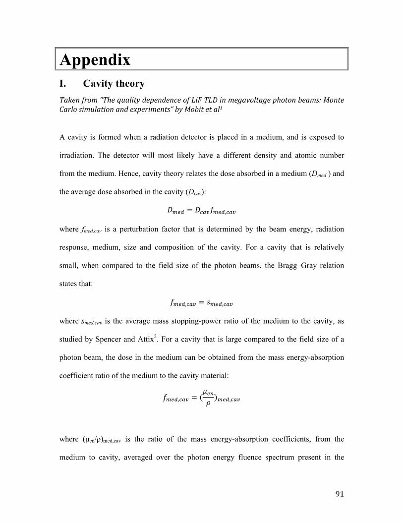
  91  

Appendix I. Cavity theory Taken  from  “The  quality  dependence  of  LiF  TLD  in  megavoltage  photon  beams:  Monte  Carlo  simulation  and  experiments”  by  Mobit  et  al1      A cavity is formed when a radiation detector is placed in a medium, and is exposed to

irradiation. The detector will most likely have a different density and atomic number

from the medium. Hence, cavity theory relates the dose absorbed in a medium (Dmed ) and

the average dose absorbed in the cavity (Dcav):

𝐷!"# = 𝐷!"#𝑓!"#,!"#

where fmed,cav is a perturbation factor that is determined by the beam energy, radiation

response, medium, size and composition of the cavity. For a cavity that is relatively

small, when compared to the field size of the photon beams, the Bragg–Gray relation

states that:

𝑓!"#,!"# = 𝑠!"#,!"#

where smed,cav is the average mass stopping-power ratio of the medium to the cavity, as

studied by Spencer and Attix2. For a cavity that is large compared to the field size of a

photon beam, the dose in the medium can be obtained from the mass energy-absorption

coefficient ratio of the medium to the cavity material:

𝑓!"#,!"# = (𝜇!"𝜌 )!"#,!"#

where (µen/ρ)med,cav is the ratio of the mass energy-absorption coefficients, from the

medium to cavity, averaged over the photon energy fluence spectrum present in the

  92  

medium. This expression ignores the perturbation effects or interface effects that may

occur by the introduction of the detector material into a different medium as it then

becomes heterogeneous medium insert3, 4.

Burlin5 theorized a general cavity theory for photons for all sizes, which approaches the

Spencer–Attix theory in the small-size limit and the ratio of the mass energy-absorption

coefficient for very large cavities. According to this theory

𝑓!"#,!"# = 𝑑𝑠!"#,!"# + (1− 𝑑)(𝜇!"𝜌 )!"#,!"#

where d is a weighting factor which gives (1−d) the contribution to the total dose from

electrons generated by photon interaction in the cavity. Burlin’s cavity equation has been

critically examined and modified by Horowitz et al6 and Almond and McCray7. These

theoretical predictions may vary considerably as they are based on empirical fits to

experimental findings.

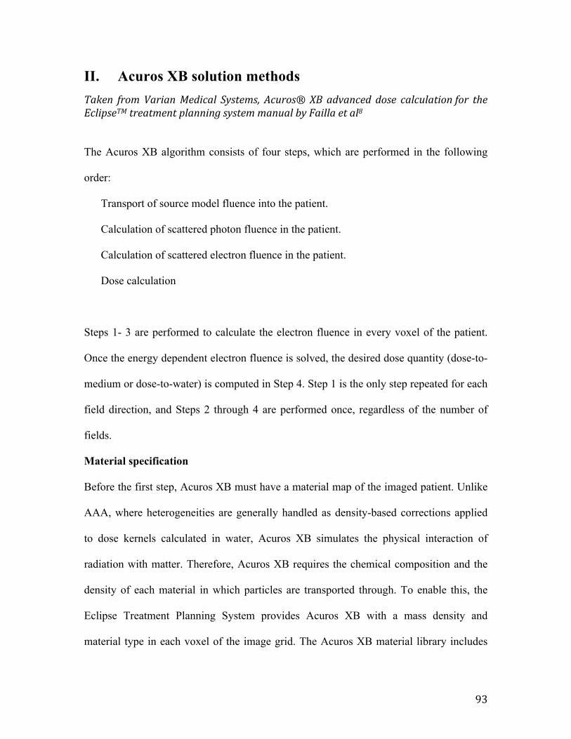
  93  

II. Acuros XB solution methods Taken   from  Varian  Medical   Systems,   Acuros®   XB   advanced   dose   calculation  for   the  EclipseTM  treatment  planning  system  manual  by  Failla  et  al8      The Acuros XB algorithm consists of four steps, which are performed in the following

order:

Transport of source model fluence into the patient.

Calculation of scattered photon fluence in the patient.

Calculation of scattered electron fluence in the patient.

Dose calculation

Steps 1- 3 are performed to calculate the electron fluence in every voxel of the patient.

Once the energy dependent electron fluence is solved, the desired dose quantity (dose-to-

medium or dose-to-water) is computed in Step 4. Step 1 is the only step repeated for each

field direction, and Steps 2 through 4 are performed once, regardless of the number of

fields.

Material specification

Before the first step, Acuros XB must have a material map of the imaged patient. Unlike

AAA, where heterogeneities are generally handled as density-based corrections applied

to dose kernels calculated in water, Acuros XB simulates the physical interaction of

radiation with matter. Therefore, Acuros XB requires the chemical composition and the

density of each material in which particles are transported through. To enable this, the

Eclipse Treatment Planning System provides Acuros XB with a mass density and

material type in each voxel of the image grid. The Acuros XB material library includes

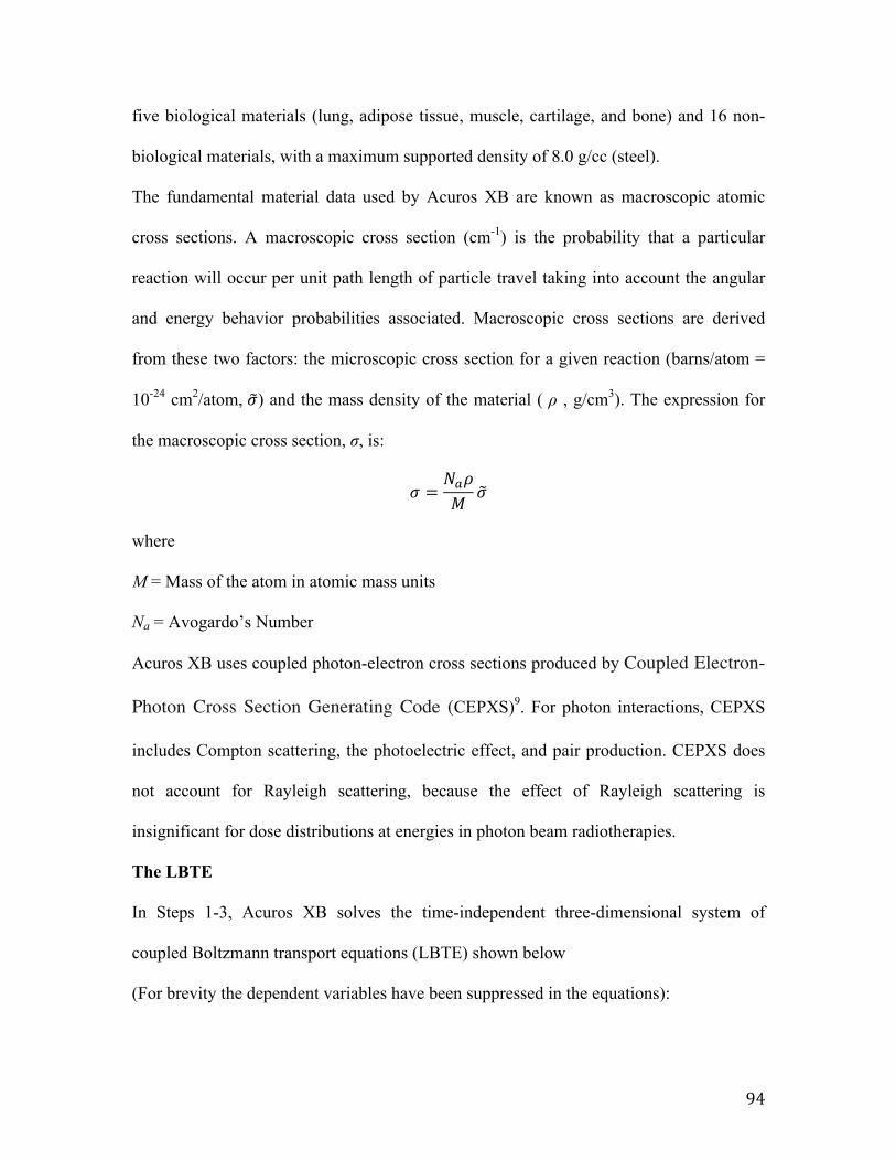
  94  

five biological materials (lung, adipose tissue, muscle, cartilage, and bone) and 16 non-

biological materials, with a maximum supported density of 8.0 g/cc (steel).

The fundamental material data used by Acuros XB are known as macroscopic atomic

cross sections. A macroscopic cross section (cm-1) is the probability that a particular

reaction will occur per unit path length of particle travel taking into account the angular

and energy behavior probabilities associated. Macroscopic cross sections are derived

from these two factors: the microscopic cross section for a given reaction (barns/atom =

10-24 cm2/atom, 𝜎) and the mass density of the material ( ρ , g/cm3). The expression for

the macroscopic cross section, σ, is:

𝜎 =𝑁!𝜌𝑀 𝜎

where

M = Mass of the atom in atomic mass units

Na = Avogardo’s Number

Acuros XB uses coupled photon-electron cross sections produced by Coupled Electron-

Photon Cross Section Generating Code (CEPXS)9. For photon interactions, CEPXS

includes Compton scattering, the photoelectric effect, and pair production. CEPXS does

not account for Rayleigh scattering, because the effect of Rayleigh scattering is

insignificant for dose distributions at energies in photon beam radiotherapies.

The LBTE

In Steps 1-3, Acuros XB solves the time-independent three-dimensional system of

coupled Boltzmann transport equations (LBTE) shown below

(For brevity the dependent variables have been suppressed in the equations):

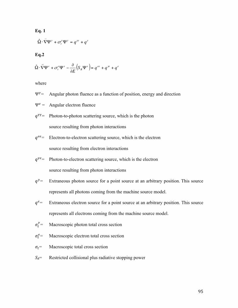
  95  

Eq. 1

Eq.2

where

Ψ!= Angular photon fluence as a function of position, energy and direction

Ψ! = Angular electron fluence

𝑞!!= Photon-to-photon scattering source, which is the photon

source resulting from photon interactions

𝑞!!= Electron-to-electron scattering source, which is the electron

source resulting from electron interactions

𝑞!"= Photon-to-electron scattering source, which is the electron

source resulting from photon interactions

𝑞!= Extraneous photon source for a point source at an arbitrary position. This source

represents all photons coming from the machine source model.

𝑞!= Extraneous electron source for a point source at an arbitrary position. This source

represents all electrons coming from the machine source model.

𝜎!!= Macroscopic photon total cross section

𝜎!!= Macroscopic electron total cross section

𝜎!= Macroscopic total cross section

SR= Restricted collisional plus radiative stopping power

2 0 | V A R I A N M E D I C A L S Y S T E M S

Acuros XB uses coupled photon-electron cross sections produced by CEPXS [ref.

4]. For photon interactions, CEPXS includes Compton scatter (also known as inco-

herent scatter), the photo-electric effect, and pair production. CEPXS does not

account for Rayleigh scatter (also known as coherent scatter), the effect of which is

insignificant for dose distributions at energies typical in photon beam radiotherapies.

The LBTE

In Steps 1 through 3, Acuros XB solves the time-independent three-dimensional

system of coupled Boltzmann transport equations (LBTE) shown below (for brevi-

ty the dependent variables have been suppressed in the equations):

Eq. 1

Eq. 2

where

= Angular photon fluence (or fluence if not time integrated), ,

as a function of position, , energy, E, and direction,

= Angular electron fluence,

= Photon-to-photon scattering source, , which is the photon

source resulting from photon interactions

= Electron-to-electron scattering source, , which is the electron

source resulting from electron interactions

= Photon-to-electron scattering source, , which is the electron

source resulting from photon interactions

= Extraneous photon source, , for point source ,

at position

This source represents all photons coming from the machine source model.

= Extraneous electron source, , for point source ,

at position

This source represents all electrons coming from the machine source model.

= Macroscopic photon total cross section, , units of cm-1

= Macroscopic electron total cross section, , units of cm-1

= Macroscopic total cross section, , units of cm-1

= Restricted collisional plus radiative stopping power, ),( ErSR!

RS

),( Ert!"t"

),( Eret

!"et"

),( Eryt

!"yt"

pr!

p)ˆ,( #Eqeeq

pr!

p)ˆ,( #Eq yyq

)ˆ,,( #Erq ye !yeq

)ˆ,,( #Erqee !eeq

)ˆ,,( #Erq yy !yyq

)ˆ,,( #$ Ere !e$

),,(ˆ %&'=#

),,( zyxr =!)ˆ,,( #$ Ery !($

( ) ,ˆ eeeeeR

eet

e qqqSE

++=$))

*$+$+,# ("!

, ˆ (((((( " qqt +=$+$+,#!

2 0 | V A R I A N M E D I C A L S Y S T E M S

Acuros XB uses coupled photon-electron cross sections produced by CEPXS [ref.

4]. For photon interactions, CEPXS includes Compton scatter (also known as inco-

herent scatter), the photo-electric effect, and pair production. CEPXS does not

account for Rayleigh scatter (also known as coherent scatter), the effect of which is

insignificant for dose distributions at energies typical in photon beam radiotherapies.

The LBTE

In Steps 1 through 3, Acuros XB solves the time-independent three-dimensional

system of coupled Boltzmann transport equations (LBTE) shown below (for brevi-

ty the dependent variables have been suppressed in the equations):

Eq. 1

Eq. 2

where

= Angular photon fluence (or fluence if not time integrated), ,

as a function of position, , energy, E, and direction,

= Angular electron fluence,

= Photon-to-photon scattering source, , which is the photon

source resulting from photon interactions

= Electron-to-electron scattering source, , which is the electron

source resulting from electron interactions

= Photon-to-electron scattering source, , which is the electron

source resulting from photon interactions

= Extraneous photon source, , for point source ,

at position

This source represents all photons coming from the machine source model.

= Extraneous electron source, , for point source ,

at position

This source represents all electrons coming from the machine source model.

= Macroscopic photon total cross section, , units of cm-1

= Macroscopic electron total cross section, , units of cm-1

= Macroscopic total cross section, , units of cm-1

= Restricted collisional plus radiative stopping power, ),( ErSR!

RS

),( Ert!"t"

),( Eret

!"et"

),( Eryt

!"yt"

pr!

p)ˆ,( #Eqeeq

pr!

p)ˆ,( #Eq yyq

)ˆ,,( #Erq ye !yeq

)ˆ,,( #Erqee !eeq

)ˆ,,( #Erq yy !yyq

)ˆ,,( #$ Ere !e$

),,(ˆ %&'=#

),,( zyxr =!)ˆ,,( #$ Ery !($

( ) ,ˆ eeeeeR

eet

e qqqSE

++=$))

*$+$+,# ("!

, ˆ (((((( " qqt +=$+$+,#!

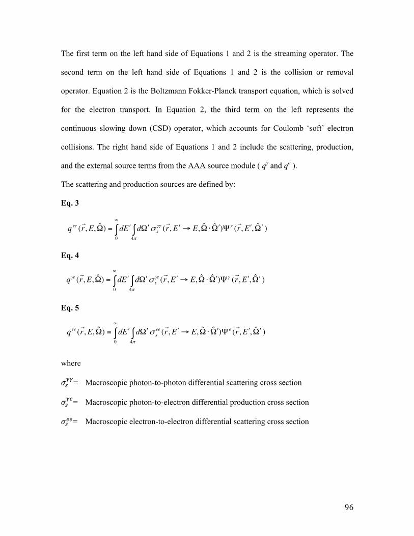
  96  

The first term on the left hand side of Equations 1 and 2 is the streaming operator. The

second term on the left hand side of Equations 1 and 2 is the collision or removal

operator. Equation 2 is the Boltzmann Fokker-Planck transport equation, which is solved

for the electron transport. In Equation 2, the third term on the left represents the

continuous slowing down (CSD) operator, which accounts for Coulomb ‘soft’ electron

collisions. The right hand side of Equations 1 and 2 include the scattering, production,

and the external source terms from the AAA source module ( qγ and qe ).

The scattering and production sources are defined by:

Eq. 3

Eq. 4

Eq. 5

where

𝜎!!!= Macroscopic photon-to-photon differential scattering cross section

𝜎!!"= Macroscopic photon-to-electron differential production cross section

𝜎!!!= Macroscopic electron-to-electron differential scattering cross section

2 1 | V A R I A N M E D I C A L S Y S T E M S

The first term on the left hand side of Equations 1 and 2 is the streaming oper-

ator. The second term on the left hand side of Equations 1 and 2 is the collision or

removal operator. Equation 2 is the Boltzmann Fokker-Planck transport equation,

which is solved for the electron transport. In Equation 2, the third term on the left

represents the continuous slowing down (CSD) operator, which accounts for

Coulomb ‘soft’ electron collisions. The right hand side of Equations 1 and 2

include the scattering, production, and the external source terms from the AAA

source module ( and ).

The scattering and production sources are defined by:

Eq. 3

’

Eq. 4

Eq. 5

where

= Macroscopic photon-to-photon differential scattering cross section

= Macroscopic photon-to-electron differential production cross section

= Macroscopic electron-to-electron differential scattering cross section

The basic assumptions used in Equations 1 and 2 are briefly summarized as fol-

lows: Both charged pair production secondary particles are assumed to be elec-

trons instead of one electron and one positron. Also, the partial coupling technique

is assumed, whereby photons can produce electrons, but electrons do not produce

photons. Regarding the latter, the energy from Bremsstrahlung photons is

assumed to be negligible and is discarded.

These assumptions have only a minor effect on the energy deposition field, and

are similar to those employed in clinical Monte Carlo codes. A primary assumption

of Equation 2 is that the Fokker-Planck operator (of which the CSD operator is

the first order term), is used for Coulomb, or “soft”, interactions that result in

small energy losses. Catastrophic interactions that result in large energy losses are

represented with the standard Boltzmann scattering. This can be seen as the deter-

ministic equivalent to electron condensed history models in Monte Carlo.

ees!

es"!

""! s

) ,ˆ,,()ˆˆ,,( )ˆ,,(40

#$$%#$&#'$#$$=# !!(

ErEErdEdErq eees

ee '''

)

!

) ,ˆ,,()ˆˆ,,( )ˆ,,(40

#$$%#$&#'$#$$=# !!(

ErEErdEdErq es

e ''' "

)

"" !

)ˆ,,()ˆˆ,,( )ˆ,,(40

#$$%#$&#'$#$$=# !!(

ErEErdEdErq s

''' "

)

"""" !

eq"q

2 1 | V A R I A N M E D I C A L S Y S T E M S

The first term on the left hand side of Equations 1 and 2 is the streaming oper-

ator. The second term on the left hand side of Equations 1 and 2 is the collision or

removal operator. Equation 2 is the Boltzmann Fokker-Planck transport equation,

which is solved for the electron transport. In Equation 2, the third term on the left

represents the continuous slowing down (CSD) operator, which accounts for

Coulomb ‘soft’ electron collisions. The right hand side of Equations 1 and 2

include the scattering, production, and the external source terms from the AAA

source module ( and ).

The scattering and production sources are defined by:

Eq. 3

’

Eq. 4

Eq. 5

where

= Macroscopic photon-to-photon differential scattering cross section

= Macroscopic photon-to-electron differential production cross section

= Macroscopic electron-to-electron differential scattering cross section

The basic assumptions used in Equations 1 and 2 are briefly summarized as fol-

lows: Both charged pair production secondary particles are assumed to be elec-

trons instead of one electron and one positron. Also, the partial coupling technique

is assumed, whereby photons can produce electrons, but electrons do not produce

photons. Regarding the latter, the energy from Bremsstrahlung photons is

assumed to be negligible and is discarded.

These assumptions have only a minor effect on the energy deposition field, and

are similar to those employed in clinical Monte Carlo codes. A primary assumption

of Equation 2 is that the Fokker-Planck operator (of which the CSD operator is

the first order term), is used for Coulomb, or “soft”, interactions that result in

small energy losses. Catastrophic interactions that result in large energy losses are

represented with the standard Boltzmann scattering. This can be seen as the deter-

ministic equivalent to electron condensed history models in Monte Carlo.

ees!

es"!

""! s

) ,ˆ,,()ˆˆ,,( )ˆ,,(40

#$$%#$&#'$#$$=# !!(

ErEErdEdErq eees

ee '''

)

!

) ,ˆ,,()ˆˆ,,( )ˆ,,(40

#$$%#$&#'$#$$=# !!(

ErEErdEdErq es

e ''' "

)

"" !

)ˆ,,()ˆˆ,,( )ˆ,,(40

#$$%#$&#'$#$$=# !!(

ErEErdEdErq s

''' "

)

"""" !

eq"q

2 1 | V A R I A N M E D I C A L S Y S T E M S

The first term on the left hand side of Equations 1 and 2 is the streaming oper-

ator. The second term on the left hand side of Equations 1 and 2 is the collision or

removal operator. Equation 2 is the Boltzmann Fokker-Planck transport equation,

which is solved for the electron transport. In Equation 2, the third term on the left

represents the continuous slowing down (CSD) operator, which accounts for

Coulomb ‘soft’ electron collisions. The right hand side of Equations 1 and 2

include the scattering, production, and the external source terms from the AAA

source module ( and ).

The scattering and production sources are defined by:

Eq. 3

’

Eq. 4

Eq. 5

where

= Macroscopic photon-to-photon differential scattering cross section

= Macroscopic photon-to-electron differential production cross section

= Macroscopic electron-to-electron differential scattering cross section

The basic assumptions used in Equations 1 and 2 are briefly summarized as fol-

lows: Both charged pair production secondary particles are assumed to be elec-

trons instead of one electron and one positron. Also, the partial coupling technique

is assumed, whereby photons can produce electrons, but electrons do not produce

photons. Regarding the latter, the energy from Bremsstrahlung photons is

assumed to be negligible and is discarded.

These assumptions have only a minor effect on the energy deposition field, and

are similar to those employed in clinical Monte Carlo codes. A primary assumption

of Equation 2 is that the Fokker-Planck operator (of which the CSD operator is

the first order term), is used for Coulomb, or “soft”, interactions that result in

small energy losses. Catastrophic interactions that result in large energy losses are

represented with the standard Boltzmann scattering. This can be seen as the deter-

ministic equivalent to electron condensed history models in Monte Carlo.

ees!

es"!

""! s

) ,ˆ,,()ˆˆ,,( )ˆ,,(40

#$$%#$&#'$#$$=# !!(

ErEErdEdErq eees

ee '''

)

!

) ,ˆ,,()ˆˆ,,( )ˆ,,(40

#$$%#$&#'$#$$=# !!(

ErEErdEdErq es

e ''' "

)

"" !

)ˆ,,()ˆˆ,,( )ˆ,,(40

#$$%#$&#'$#$$=# !!(

ErEErdEdErq s

''' "

)

"""" !

eq"q

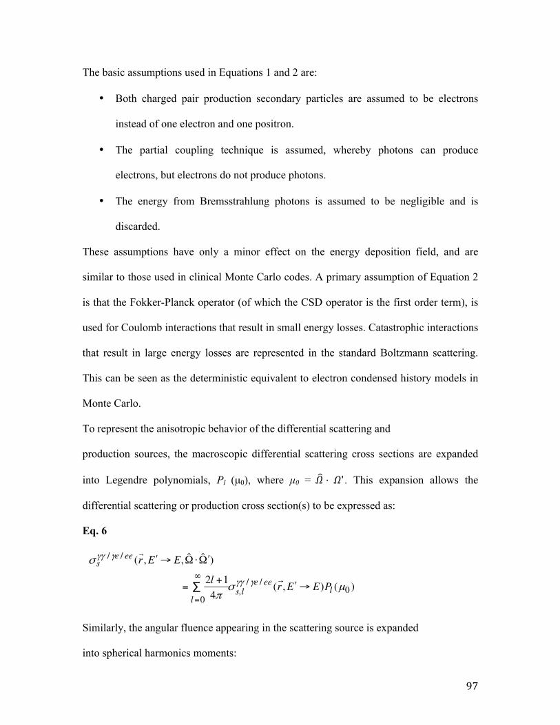
  97  

The basic assumptions used in Equations 1 and 2 are:

• Both charged pair production secondary particles are assumed to be electrons

instead of one electron and one positron.

• The partial coupling technique is assumed, whereby photons can produce

electrons, but electrons do not produce photons.

• The energy from Bremsstrahlung photons is assumed to be negligible and is

discarded.

These assumptions have only a minor effect on the energy deposition field, and are

similar to those used in clinical Monte Carlo codes. A primary assumption of Equation 2

is that the Fokker-Planck operator (of which the CSD operator is the first order term), is

used for Coulomb interactions that result in small energy losses. Catastrophic interactions

that result in large energy losses are represented in the standard Boltzmann scattering.

This can be seen as the deterministic equivalent to electron condensed history models in

Monte Carlo.

To represent the anisotropic behavior of the differential scattering and

production sources, the macroscopic differential scattering cross sections are expanded

into Legendre polynomials, Pl (µ0), where µ0 = 𝛺 ⋅  𝛺ʹ. This expansion allows the

differential scattering or production cross section(s) to be expressed as:

Eq. 6

Similarly, the angular fluence appearing in the scattering source is expanded

into spherical harmonics moments:

2 2 | V A R I A N M E D I C A L S Y S T E M S

To represent the anisotropic behavior of the differential scattering and

production sources, in a mathematically practical manner, the macroscopic

differential scattering cross sections are expanded into Legendre polynomials,

, where . This expansion allows the differential scattering

or production cross section(s) to be expressed as:

Eq. 6

,

Similarly, the angular fluence appearing in the scattering source is expanded

into spherical harmonics moments:

Eq. 7

where

= Spherical harmonic functions

= Angular indices

= Spherical harmonics moments of the angular fluence, calculated as:

where * denotes the complex conjugate

= Macroscopic electron-to-electron differential scattering cross section

Equations 6 and 7 are exact. Additionally, for purely isotropic scattering, l = 0

is also exact. However, Acuros XB sets a limit on the scattering order, l !7, and

hence the number of spherical harmonic moments kept in the scattering/produc-

tion source. Using the Legendre addition theorem, the scattering and production

sources become:

Eq. 8

! ! "= !=

"

#$=

#7

0 0,,

//,

//

).ˆ('),()',('

)ˆ,,(

l

l

lmmlml

eeels

eee

YErEErdE

Erq

$$

$

%& '''

'''

ees&

),'ˆ,()ˆ('4

*," #(#)#

*

,ErYd ml$

),(, Erml )$%

ml,

)ˆ(, #mlY

)ˆ(),()ˆ,,( ,0

, #))=#))( ! !"

= !=ml

l

l

lmml YErEr

$$% ,

)(),(4

12

)ˆˆ,,(

0//

0

//

+&*

&

'''

'''

leee

s,ll

eees

PEErl

EEr

$)+

=

#),#$)

!"

=

$

$

#),#= ˆ0+)( 0+lP

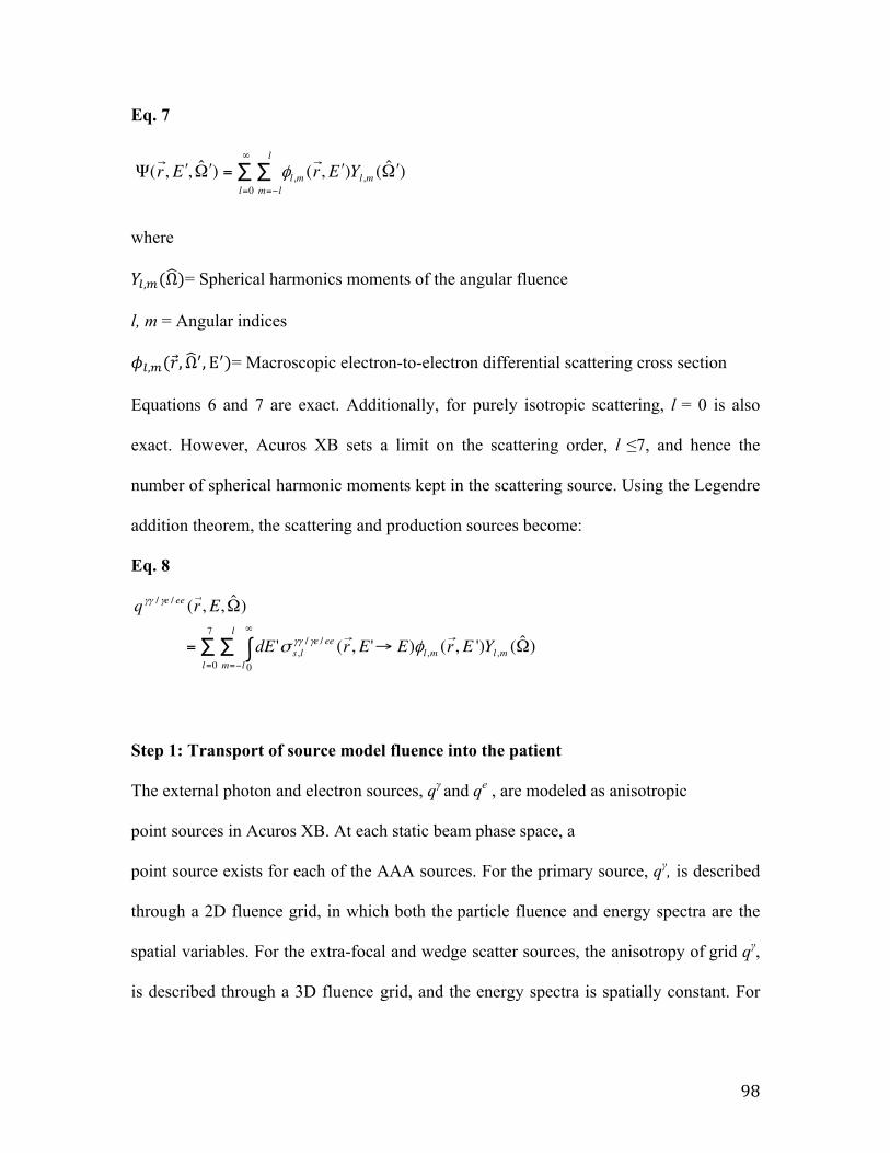
  98  

Eq. 7

where

𝑌!,!(Ω)= Spherical harmonics moments of the angular fluence

l, m = Angular indices

𝜙!,!(𝑟,Ω!,E!)= Macroscopic electron-to-electron differential scattering cross section

Equations 6 and 7 are exact. Additionally, for purely isotropic scattering, l = 0 is also

exact. However, Acuros XB sets a limit on the scattering order, l ≤7, and hence the

number of spherical harmonic moments kept in the scattering source. Using the Legendre

addition theorem, the scattering and production sources become:

Eq. 8

Step 1: Transport of source model fluence into the patient

The external photon and electron sources, qγ and qe , are modeled as anisotropic

point sources in Acuros XB. At each static beam phase space, a

point source exists for each of the AAA sources. For the primary source, qγ, is described

through a 2D fluence grid, in which both the particle fluence and energy spectra are the

spatial variables. For the extra-focal and wedge scatter sources, the anisotropy of grid qγ,

is described through a 3D fluence grid, and the energy spectra is spatially constant. For

2 2 | V A R I A N M E D I C A L S Y S T E M S

To represent the anisotropic behavior of the differential scattering and

production sources, in a mathematically practical manner, the macroscopic

differential scattering cross sections are expanded into Legendre polynomials,

, where . This expansion allows the differential scattering

or production cross section(s) to be expressed as:

Eq. 6

,

Similarly, the angular fluence appearing in the scattering source is expanded

into spherical harmonics moments:

Eq. 7

where

= Spherical harmonic functions

= Angular indices

= Spherical harmonics moments of the angular fluence, calculated as:

where * denotes the complex conjugate

= Macroscopic electron-to-electron differential scattering cross section

Equations 6 and 7 are exact. Additionally, for purely isotropic scattering, l = 0

is also exact. However, Acuros XB sets a limit on the scattering order, l !7, and

hence the number of spherical harmonic moments kept in the scattering/produc-

tion source. Using the Legendre addition theorem, the scattering and production

sources become:

Eq. 8

! ! "= !=

"

#$=

#7

0 0,,

//,

//

).ˆ('),()',('

)ˆ,,(

l

l

lmmlml

eeels

eee

YErEErdE

Erq

$$

$

%& '''

'''

ees&

),'ˆ,()ˆ('4

*," #(#)#

*

,ErYd ml$

),(, Erml )$%

ml,

)ˆ(, #mlY

)ˆ(),()ˆ,,( ,0

, #))=#))( ! !"

= !=ml

l

l

lmml YErEr

$$% ,

)(),(4

12

)ˆˆ,,(

0//

0

//

+&*

&

'''

'''

leee

s,ll

eees

PEErl

EEr

$)+

=

#),#$)

!"

=

$

$

#),#= ˆ0+)( 0+lP

2 2 | V A R I A N M E D I C A L S Y S T E M S

To represent the anisotropic behavior of the differential scattering and

production sources, in a mathematically practical manner, the macroscopic

differential scattering cross sections are expanded into Legendre polynomials,

, where . This expansion allows the differential scattering

or production cross section(s) to be expressed as:

Eq. 6

,

Similarly, the angular fluence appearing in the scattering source is expanded

into spherical harmonics moments:

Eq. 7

where

= Spherical harmonic functions

= Angular indices

= Spherical harmonics moments of the angular fluence, calculated as:

where * denotes the complex conjugate

= Macroscopic electron-to-electron differential scattering cross section

Equations 6 and 7 are exact. Additionally, for purely isotropic scattering, l = 0

is also exact. However, Acuros XB sets a limit on the scattering order, l !7, and

hence the number of spherical harmonic moments kept in the scattering/produc-

tion source. Using the Legendre addition theorem, the scattering and production

sources become:

Eq. 8

! ! "= !=

"

#$=

#7

0 0,,

//,

//

).ˆ('),()',('

)ˆ,,(

l

l

lmmlml

eeels

eee

YErEErdE

Erq

$$

$

%& '''

'''

ees&

),'ˆ,()ˆ('4

*," #(#)#

*

,ErYd ml$

),(, Erml )$%

ml,

)ˆ(, #mlY

)ˆ(),()ˆ,,( ,0

, #))=#))( ! !"

= !=ml

l

l

lmml YErEr

$$% ,

)(),(4

12

)ˆˆ,,(

0//

0

//

+&*

&

'''

'''

leee

s,ll

eees

PEErl

EEr

$)+

=

#),#$)

!"

=

$

$

#),#= ˆ0+)( 0+lP

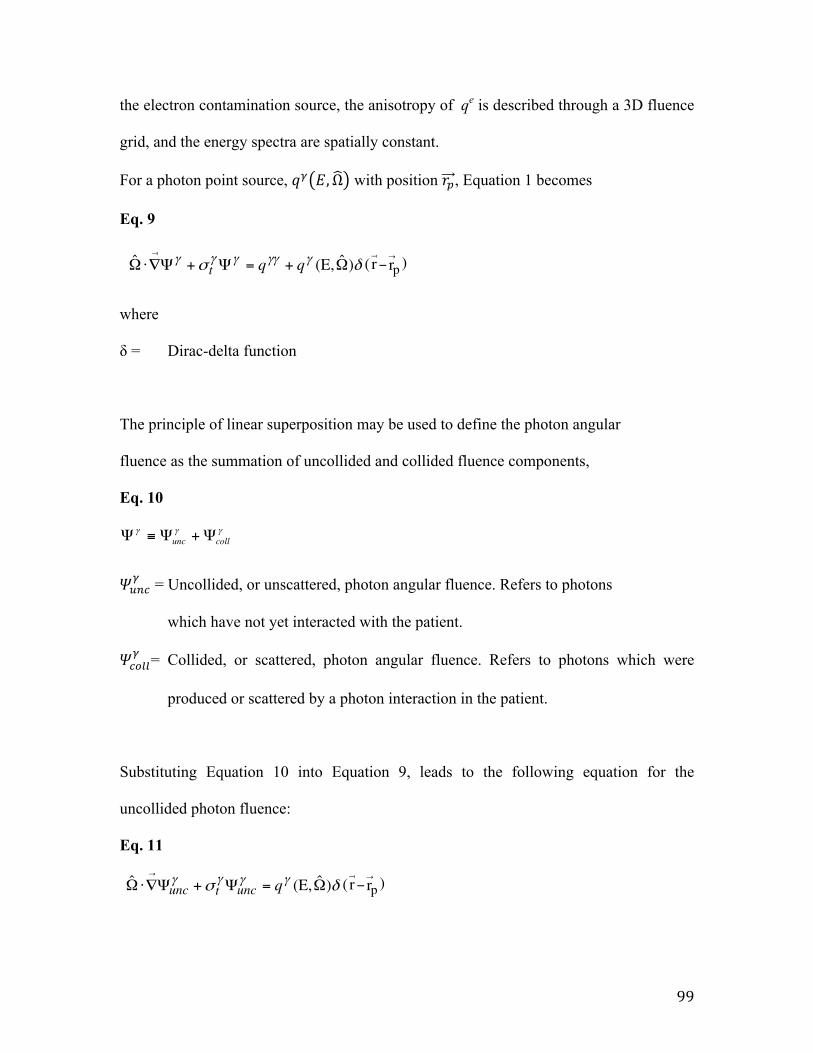
  99  

the electron contamination source, the anisotropy of qe is described through a 3D fluence

grid, and the energy spectra are spatially constant.

For a photon point source, 𝑞! 𝐸,Ω with position 𝑟!, Equation 1 becomes

Eq. 9

where

δ = Dirac-delta function

The principle of linear superposition may be used to define the photon angular

fluence as the summation of uncollided and collided fluence components,

Eq. 10

𝛹!"#! = Uncollided, or unscattered, photon angular fluence. Refers to photons

which have not yet interacted with the patient.

𝛹!"##! = Collided, or scattered, photon angular fluence. Refers to photons which were

produced or scattered by a photon interaction in the patient.

Substituting Equation 10 into Equation 9, leads to the following equation for the

uncollided photon fluence:

Eq. 11

2 3 | V A R I A N M E D I C A L S Y S T E M S

Step 1: Transport of source model fluence into the patient

The external photon and electron sources, and , are modeled as anisotropic

point sources in Acuros XB. At each static beam phase space (i.e. control point), a

separate point source exists for each of the AAA sources. For the primary source,

the anisotropy of is described through a 2D fluence grid, in which both the

particle fluence and energy spectra are spatially variable. For the extra-focal and

wedge scatter sources, the anisotropy of is described through a 3D fluence

grid, and the energy spectra is spatially constant. For the electron contamination

source, the anisotropy of is described through a 3D fluence grid, and the ener-

gy spectra is spatially constant. All point sources are located at the target for the

respective control point.

For a photon point source, located at position, , Equation 1

becomes:

Eq. 9

where

= Dirac-delta function

The principle of linear superposition may be used to define the photon angular

fluence as the summation of uncollided and collided fluence components,

Eq. 10

,

where

= Uncollided, or unscattered, photon angular fluence. Refers to photons

which have not yet interacted with the patient/phantom.

= Collided, or scattered, photon angular fluence. Refers to photons which

were produced or scattered by a photon interaction in the patient/

phantom.

Substituting Equation 10 into Equation 9, leads to the following equation for

the uncollided photon fluence:

Eq. 11

)ˆ(E,ˆ!

"# $$$$ %=&+&'(% qunctunc , rp!

r!

( ))

$coll&

$unc&

$$$collunc &+&*&

"

,r)ˆ(E,ˆp!!

"# $$$$$$ %+=&+&'(% qqt r!

( ))

pr!

ˆ,( %)Eq$

eq

yq

yq

eqyq

2 3 | V A R I A N M E D I C A L S Y S T E M S

Step 1: Transport of source model fluence into the patient

The external photon and electron sources, and , are modeled as anisotropic

point sources in Acuros XB. At each static beam phase space (i.e. control point), a

separate point source exists for each of the AAA sources. For the primary source,

the anisotropy of is described through a 2D fluence grid, in which both the

particle fluence and energy spectra are spatially variable. For the extra-focal and

wedge scatter sources, the anisotropy of is described through a 3D fluence

grid, and the energy spectra is spatially constant. For the electron contamination

source, the anisotropy of is described through a 3D fluence grid, and the ener-

gy spectra is spatially constant. All point sources are located at the target for the

respective control point.

For a photon point source, located at position, , Equation 1

becomes:

Eq. 9

where

= Dirac-delta function

The principle of linear superposition may be used to define the photon angular

fluence as the summation of uncollided and collided fluence components,

Eq. 10

,

where

= Uncollided, or unscattered, photon angular fluence. Refers to photons

which have not yet interacted with the patient/phantom.

= Collided, or scattered, photon angular fluence. Refers to photons which

were produced or scattered by a photon interaction in the patient/

phantom.

Substituting Equation 10 into Equation 9, leads to the following equation for

the uncollided photon fluence:

Eq. 11

)ˆ(E,ˆ!

"# $$$$ %=&+&'(% qunctunc , rp!

r!

( ))

$coll&

$unc&

$$$collunc &+&*&

"

,r)ˆ(E,ˆp!!

"# $$$$$$ %+=&+&'(% qqt r!

( ))

pr!

ˆ,( %)Eq$

eq

yq

yq

eqyq

2 3 | V A R I A N M E D I C A L S Y S T E M S

Step 1: Transport of source model fluence into the patient

The external photon and electron sources, and , are modeled as anisotropic

point sources in Acuros XB. At each static beam phase space (i.e. control point), a

separate point source exists for each of the AAA sources. For the primary source,

the anisotropy of is described through a 2D fluence grid, in which both the

particle fluence and energy spectra are spatially variable. For the extra-focal and

wedge scatter sources, the anisotropy of is described through a 3D fluence

grid, and the energy spectra is spatially constant. For the electron contamination

source, the anisotropy of is described through a 3D fluence grid, and the ener-

gy spectra is spatially constant. All point sources are located at the target for the

respective control point.

For a photon point source, located at position, , Equation 1

becomes:

Eq. 9

where

= Dirac-delta function

The principle of linear superposition may be used to define the photon angular

fluence as the summation of uncollided and collided fluence components,

Eq. 10

,

where

= Uncollided, or unscattered, photon angular fluence. Refers to photons

which have not yet interacted with the patient/phantom.

= Collided, or scattered, photon angular fluence. Refers to photons which

were produced or scattered by a photon interaction in the patient/

phantom.

Substituting Equation 10 into Equation 9, leads to the following equation for

the uncollided photon fluence:

Eq. 11

)ˆ(E,ˆ!

"# $$$$ %=&+&'(% qunctunc , rp!

r!

( ))

$coll&

$unc&

$$$collunc &+&*&

"

,r)ˆ(E,ˆp!!

"# $$$$$$ %+=&+&'(% qqt r!

( ))

pr!

ˆ,( %)Eq$

eq

yq

yq

eqyq

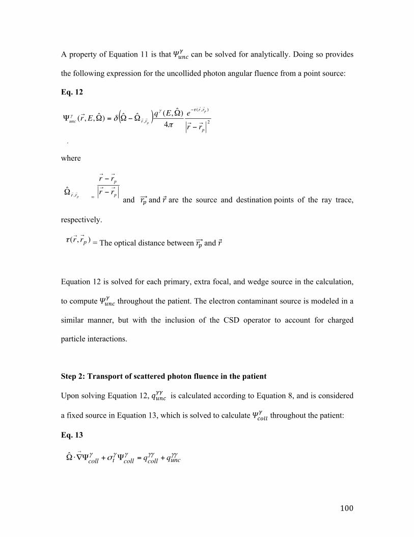
  100  

A property of Equation 11 is that 𝛹!"#! can be solved for analytically. Doing so provides

the following expression for the uncollided photon angular fluence from a point source:

Eq. 12

where

and 𝑟!  and 𝑟 are the source and destination points of the ray trace,

respectively.

= The optical distance between 𝑟!  and 𝑟

Equation 12 is solved for each primary, extra focal, and wedge source in the calculation,

to compute 𝛹!"#! throughout the patient. The electron contaminant source is modeled in a

similar manner, but with the inclusion of the CSD operator to account for charged

particle interactions.

Step 2: Transport of scattered photon fluence in the patient

Upon solving Equation 12, 𝑞!"#!! is calculated according to Equation 8, and is considered

a fixed source in Equation 13, which is solved to calculate 𝛹!"##! throughout the patient:

Eq. 13

2 4 | V A R I A N M E D I C A L S Y S T E M S

A property of Equation 11 is that can be solved for analytically. Doing

so provides the following expression for the uncollided photon angular fluence

from a point source:

Eq. 12

,

where

= , where and are the source and destination

points of the ray trace, respectively.

= The optical distance (measured in mean-free-paths) between and .

Equation 12 is solved for each primary, extra focal, and wedge source in the cal-

culation, to compute throughout the patient. The electron contaminant

source is modeled in a similar manner, but with the inclusion of the CSD operator

to account for charged particle interactions.

Step 2: Transport of scattered photon fluence in the patient

Once Equation 12 is solved, is calculated according to Equation 8, and is

considered a fixed source in Equation 13, which is solved to compute

throughout the patient:

Eq. 13

where

= First scattered photon source. Refers to photons which are created or scat-

tered from the first photon interaction inside the patient/phantom.

= Secondary scattered photon source. Refers to photons which are created or

scattered from secondary photon interactions inside the patient/phantom.

yycollq

yyuncq

, ˆ !!!!!!! " unccollcolltcoll qq +=#+#$%&'

!coll#

!!uncq

!unc#

pr'

r'),( prr

''(

r'

pr'

p

p

rr

rr''

''

)

)

prr''

,&̂

( )2

),(

, 4)ˆ,(ˆˆ)ˆ,,(

p

rr

rruncrr

eEqEr

p

p ''

'

''

''

)

&&)&=&#

)(!!

*+

!unc#

2 4 | V A R I A N M E D I C A L S Y S T E M S

A property of Equation 11 is that can be solved for analytically. Doing

so provides the following expression for the uncollided photon angular fluence

from a point source:

Eq. 12

,

where

= , where and are the source and destination

points of the ray trace, respectively.

= The optical distance (measured in mean-free-paths) between and .

Equation 12 is solved for each primary, extra focal, and wedge source in the cal-

culation, to compute throughout the patient. The electron contaminant

source is modeled in a similar manner, but with the inclusion of the CSD operator

to account for charged particle interactions.

Step 2: Transport of scattered photon fluence in the patient

Once Equation 12 is solved, is calculated according to Equation 8, and is

considered a fixed source in Equation 13, which is solved to compute

throughout the patient:

Eq. 13

where

= First scattered photon source. Refers to photons which are created or scat-

tered from the first photon interaction inside the patient/phantom.

= Secondary scattered photon source. Refers to photons which are created or

scattered from secondary photon interactions inside the patient/phantom.

yycollq

yyuncq

, ˆ !!!!!!! " unccollcolltcoll qq +=#+#$%&'

!coll#

!!uncq

!unc#

pr'

r'),( prr

''(

r'

pr'

p

p

rr

rr''

''

)

)

prr''

,&̂

( )2

),(

, 4)ˆ,(ˆˆ)ˆ,,(

p

rr

rruncrr

eEqEr

p

p ''

'

''

''

)

&&)&=&#

)(!!

*+

!unc#

2 4 | V A R I A N M E D I C A L S Y S T E M S

A property of Equation 11 is that can be solved for analytically. Doing

so provides the following expression for the uncollided photon angular fluence

from a point source:

Eq. 12

,

where

= , where and are the source and destination

points of the ray trace, respectively.

= The optical distance (measured in mean-free-paths) between and .

Equation 12 is solved for each primary, extra focal, and wedge source in the cal-

culation, to compute throughout the patient. The electron contaminant

source is modeled in a similar manner, but with the inclusion of the CSD operator

to account for charged particle interactions.

Step 2: Transport of scattered photon fluence in the patient

Once Equation 12 is solved, is calculated according to Equation 8, and is

considered a fixed source in Equation 13, which is solved to compute

throughout the patient:

Eq. 13

where

= First scattered photon source. Refers to photons which are created or scat-

tered from the first photon interaction inside the patient/phantom.

= Secondary scattered photon source. Refers to photons which are created or

scattered from secondary photon interactions inside the patient/phantom.

yycollq

yyuncq

, ˆ !!!!!!! " unccollcolltcoll qq +=#+#$%&'

!coll#

!!uncq

!unc#

pr'

r'),( prr

''(

r'

pr'

p

p

rr

rr''

''

)

)

prr''

,&̂

( )2

),(

, 4)ˆ,(ˆˆ)ˆ,,(

p

rr

rruncrr

eEqEr

p

p ''

'

''

''

)

&&)&=&#

)(!!

*+

!unc#

2 4 | V A R I A N M E D I C A L S Y S T E M S

A property of Equation 11 is that can be solved for analytically. Doing

so provides the following expression for the uncollided photon angular fluence

from a point source:

Eq. 12

,

where

= , where and are the source and destination

points of the ray trace, respectively.

= The optical distance (measured in mean-free-paths) between and .

Equation 12 is solved for each primary, extra focal, and wedge source in the cal-

culation, to compute throughout the patient. The electron contaminant

source is modeled in a similar manner, but with the inclusion of the CSD operator

to account for charged particle interactions.

Step 2: Transport of scattered photon fluence in the patient

Once Equation 12 is solved, is calculated according to Equation 8, and is

considered a fixed source in Equation 13, which is solved to compute

throughout the patient:

Eq. 13

where

= First scattered photon source. Refers to photons which are created or scat-

tered from the first photon interaction inside the patient/phantom.

= Secondary scattered photon source. Refers to photons which are created or

scattered from secondary photon interactions inside the patient/phantom.

yycollq

yyuncq

, ˆ !!!!!!! " unccollcolltcoll qq +=#+#$%&'

!coll#

!!uncq

!unc#

pr'

r'),( prr

''(

r'

pr'

p

p

rr

rr''

''

)

)

prr''

,&̂

( )2

),(

, 4)ˆ,(ˆˆ)ˆ,,(

p

rr

rruncrr

eEqEr

p

p ''

'

''

''

)

&&)&=&#

)(!!

*+

!unc#

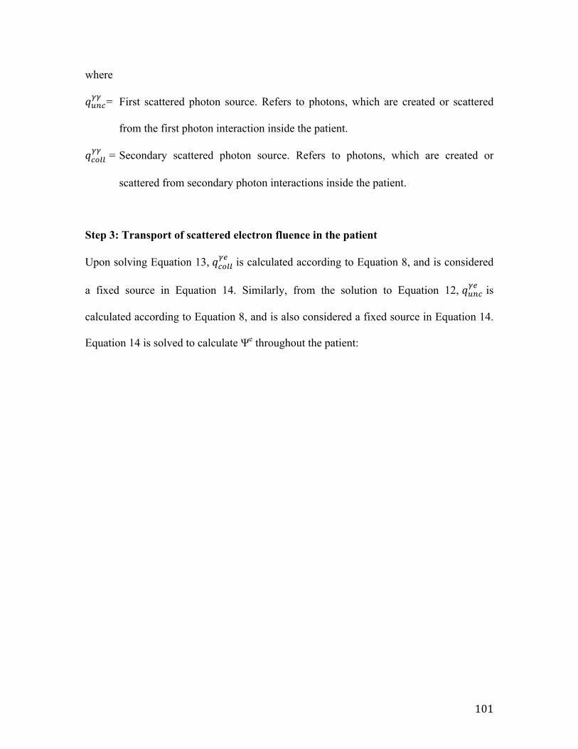
  101  

where

𝑞!"#!! = First scattered photon source. Refers to photons, which are created or scattered

from the first photon interaction inside the patient.

𝑞!"##!! = Secondary scattered photon source. Refers to photons, which are created or

scattered from secondary photon interactions inside the patient.

Step 3: Transport of scattered electron fluence in the patient

Upon solving Equation 13, 𝑞!"##!" is calculated according to Equation 8, and is considered

a fixed source in Equation 14. Similarly, from the solution to Equation 12, 𝑞!"#!" is

calculated according to Equation 8, and is also considered a fixed source in Equation 14.

Equation 14 is solved to calculate Ψe throughout the patient:

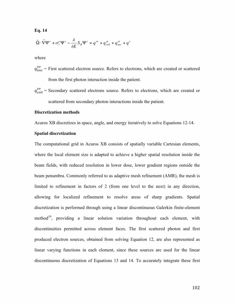
  102  

Eq. 14

where

𝑞!"#!" = First scattered electron source. Refers to electrons, which are created or scattered

from the first photon interaction inside the patient.

𝑞!"##!" = Secondary scattered electrons source. Refers to electrons, which are created or

scattered from secondary photon interactions inside the patient.

Discretization methods

Acuros XB discretizes in space, angle, and energy iteratively to solve Equations 12-14.

Spatial discretization

The computational grid in Acuros XB consists of spatially variable Cartesian elements,

where the local element size is adapted to achieve a higher spatial resolution inside the

beam fields, with reduced resolution in lower dose, lower gradient regions outside the

beam penumbra. Commonly referred to as adaptive mesh refinement (AMR), the mesh is

limited to refinement in factors of 2 (from one level to the next) in any direction,

allowing for localized refinement to resolve areas of sharp gradients. Spatial

discretization is performed through using a linear discontinuous Galerkin finite-element

method10, providing a linear solution variation throughout each element, with

discontinuities permitted across element faces. The first scattered photon and first

produced electron sources, obtained from solving Equation 12, are also represented as

linear varying functions in each element, since these sources are used for the linear

discontinuous discretization of Equations 13 and 14. To accurately integrate these first

2 5 | V A R I A N M E D I C A L S Y S T E M S

Step 3: Transport of scattered electron fluence in the patient

Once Equation 13 is solved, is calculated according to Equation 8, and is

considered a fixed source in Equation 14. Similarly, from the solution to Equation

12, is calculated according to Equation 8, and is also considered a fixed

source in Equation 14. Equation 14 is solved to compute throughout the

patient:

Eq. 14

where

= First scattered electron source. Refers to electrons which are created or scat-

tered from the first photon interaction inside the patient/phantom.

= Secondary scattered electrons source. Refers to electrons which are created

or scattered from secondary photon interactions inside the patient/phan-

tom.

Discretization methods

Acuros XB discretizes in space, angle, and energy to iteratively solve Equations 12

through 14, the methods of which are discussed below.

Spatial discretization

The computational grid in Acuros XB consists of spatially variable Cartesian ele-

ments, where the local element size is adapted to achieve a higher spatial resolution

inside the beam fields, with reduced resolution in lower dose, lower gradient

regions outside the beam penumbra. Commonly referred to as adaptive mesh

refinement (AMR), the mesh is limited to refinement in factors of 2 (from one

level to the next) in any direction, allowing for localized refinement to resolve areas

of sharp gradients. Spatial discretization is performed through using a linear dis-

continuous Galerkin finite-element method [ref. 1], providing a linear solution

variation throughout each element, with discontinuities permitted across element

faces. The first scattered photon and first produced electron sources, obtained from

solving Equation 12, are also represented as linear varying functions in each ele-

ment, since these sources are used for the linear discontinuous discretization of

Equations 13 and 14. To accurately integrate these first scattered sources, the ana-

lytic solution is computed at a density inside the primary beam and penumbras of

at least 8 ray traces per output grid voxel.

yecollq

yeuncq

, ˆ eeunc

ecoll

eeeR

eet

e qqqqSE

+++=!""

#!+!$%& ''()

e!

yeuncq

yecollq

  103  

scattered sources, the analytic solution is computed at a density inside the primary beam

and penumbras of at least 8 ray traces per output grid voxel.

Energy discretization

Energy discretization is performed through the standard multigroup method10, which is

used in both the energy dependence of Equations 12 and 13 and the Boltzmann scattering

in Equation 14. In energy, the energy derivative of the continuous slowing down (CSD)

operator in Equation 14 is discretized using the linear discontinuous finite-element

method11. The Acuros XB cross section library includes 25 photon energy groups and 49

electron energy groups, although not all groups are used for energies lower than 20 MV.

Angular discretization

For the spatial transport of the scattered particle field, the discrete ordinates method is

used to discretize in angle10. The discrete ordinates method consists of requiring

Equations 13 and 14 to hold for a fixed number of directions, Ω! . These discrete

directions are chosen from an angular quadrature set that also serves to compute the

angular integrals in Equation 5 for the generation of the scattering source. Square-

Tchebyshev legendre quadrature sets are used and the quadrature order ranges from N=4

(32 discrete angles) to N=16 (512 discrete angles). The angular quadrature order varies

both by particle type and energy. Higher energy particles have longer mean free paths, or

ranges for electrons, and thus for each particle type, the angular quadrature order is

increased with the particle energy.

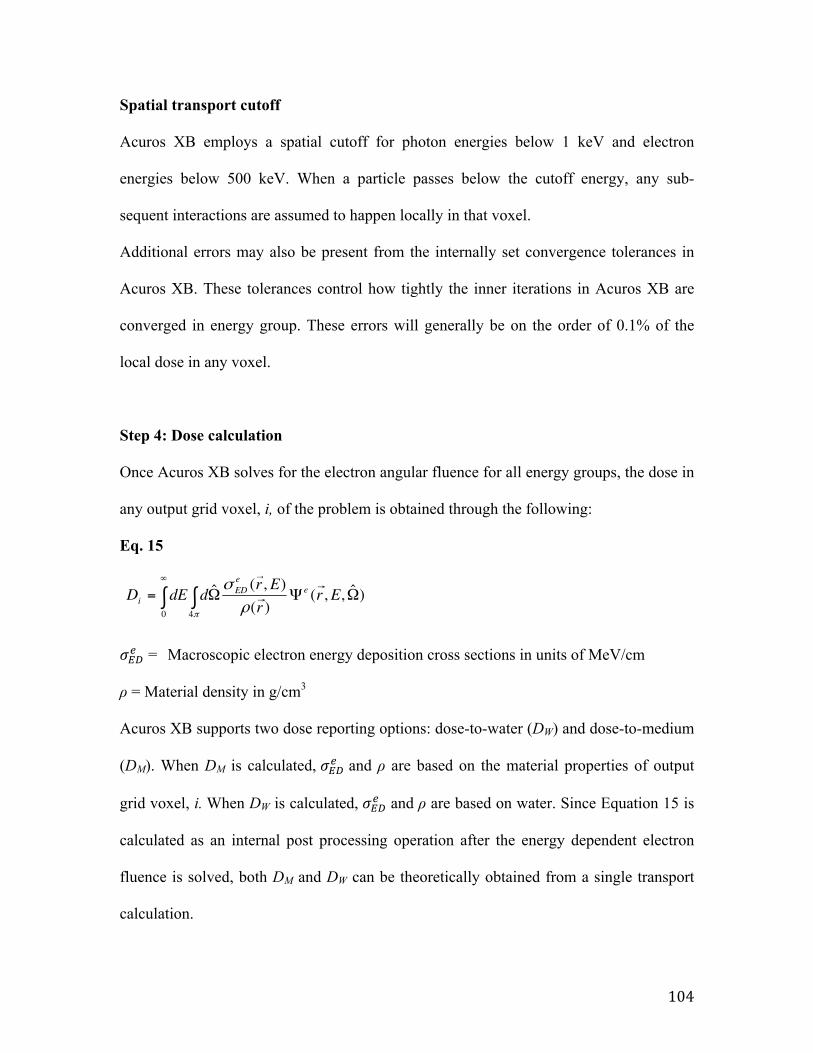
  104  

Spatial transport cutoff

Acuros XB employs a spatial cutoff for photon energies below 1 keV and electron

energies below 500 keV. When a particle passes below the cutoff energy, any sub-

sequent interactions are assumed to happen locally in that voxel.

Additional errors may also be present from the internally set convergence tolerances in

Acuros XB. These tolerances control how tightly the inner iterations in Acuros XB are

converged in energy group. These errors will generally be on the order of 0.1% of the

local dose in any voxel.

Step 4: Dose calculation

Once Acuros XB solves for the electron angular fluence for all energy groups, the dose in

any output grid voxel, i, of the problem is obtained through the following:

Eq. 15

𝜎!"! = Macroscopic electron energy deposition cross sections in units of MeV/cm

ρ = Material density in g/cm3

Acuros XB supports two dose reporting options: dose-to-water (DW) and dose-to-medium

(DM). When DM is calculated, 𝜎!"! and ρ are based on the material properties of output

grid voxel, i. When DW is calculated, 𝜎!"! and ρ are based on water. Since Equation 15 is

calculated as an internal post processing operation after the energy dependent electron

fluence is solved, both DM and DW can be theoretically obtained from a single transport

calculation.

2 7 | V A R I A N M E D I C A L S Y S T E M S

Step 4: Dose calculation

Once Acuros XB solves for the electron angular fluence for all energy groups, the

dose in any output grid voxel, i, of the problem is obtained through the following:

Eq. 15

,

where

= Macroscopic electron energy deposition cross sections in units of MeV/cm

= Material density in g/cm3

Acuros XB supports two dose reporting options: dose-to-water (DW) and dose-

to-medium (DM). When DM is calculated, and are based on the materi-

al properties of output grid voxel, i. When DW is calculated, and are

based on water. Since Equation 15 is calculated as an internal post processing oper-

ation after the energy dependent electron fluence is solved, both DM and DW can

be theoretically obtained from a single transport calculation.

!eED"

!eED"

!

eED"

)ˆ,,()(

),(ˆ40

#$#= !!%

Err

ErddED e

eED

i

&

&

&

!"

'

  105  

III. Appendix References 1.   P.  N.  Mobit,  P.  Mayles,  Alan  E  Nahum,  Joint  Department  of  Physics,  Institute  of  

Cancer  Research  and  Royal  Marsden  NHS  Trust,  Sutton  and  U.  SM2  5PT,  Phys.  Med.  Biol.  41,  387-­‐398  (1996).  

2.   L.  V.  Spencer  and  F.  H.  Attix,  Radiat.  Res.  3,  239-­‐254  (1955).  3.   A.  G.  Carlsson,  Acta  Radiol.  Suppl.  (332)  (1973).  4.   G.  Bertilsson,  University  of  Lund,  1975.  5.   T.  E.  Burlin,  Br.  J.  Radiol.  39,  727-­‐734  (1966).  6.   Y.   S.   Horowitz,   M.   Moscovith   and   A.   Dubi,   Phys.   Med.   Biol.   28,   829-­‐840  

(1983).  7.   P.  R.  Almond  and  K.  McCray,  Phys.  Med.  Biol.  15,  355-­‐342  (1970).  8.   G.  A.  Failla,  T.  Wareing,  Y.  Archambault  and  S.  Thompson,  California,  USA.  9.   L.  Lorence,  J.  Morel  and  G.  Valdez,  SAND89-­‐1685,Sandia  National  Laboratory  

(1989).  10.   E.  E.  Lewis  and  W.  F.  Miller,  Wiley,  New  York  (1984).  11.   T.  A.  Wareing,  J.  E.  Morel  and  J.  M.  McGhee,  Trans  Am.  Nucl.  Soc.,  Washington  

D.C.  83  (2000).