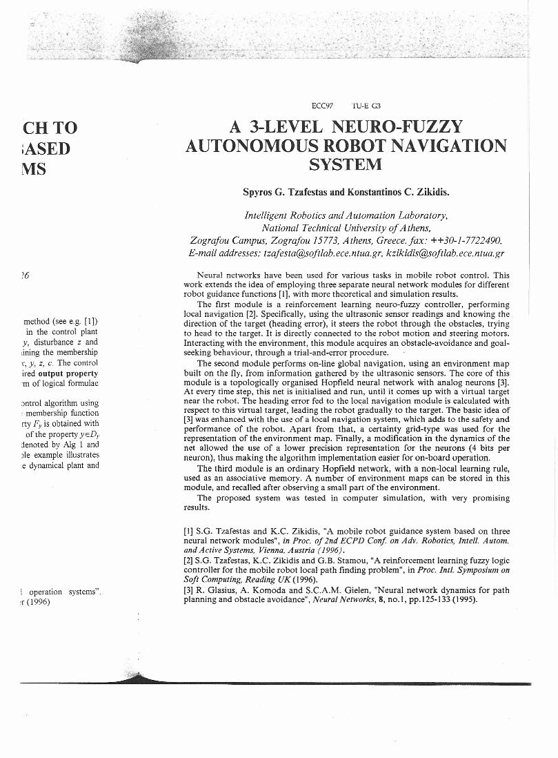
A three-level neurofuzzy autonomous navigation system
7
" ., 1; ~, .• -=:~~~ -~=~- ~::.* '-<-- CHTO :ASED MS ?6 method (see e.g, [1]) in the control plant y, disturbance z and .ining the membership r, y, z, c. The control ired output property 'm of logical formulae ontrol algorithm using : membership function rty F, is obtained with of the property y=D; jenoted by AJg 1 and ole example illustrates re dynamical plant and 1 operation systems", .r (1996) ", -,' ECC97 TIJ-E G3 A 3-LEVEL NEURO-FUZZY AUTONOMOUS ROBOT NAVIGATION SYSTEM Spyros G. Tzafestas and Konstantinos C. Zikidis. Intelligent Robolics and Automation Laboratory, National Technical University of A thens, Zografou Campus, Zografou 15773, Athens, Greece.fax: ++30-1-7722490, E-mail addresses: [email protected], [email protected] Neural networks have been used for various tasks in mobile robot control. This work extends the idea of employing three separate neural network modules for different robot guidance functions [1], with more theoretical and simulation results. The first module is a reinforcement learning neuro-fuzzy controller, performing local navigation [2]. Specifically, using the ultrasonic sensor readings and knowing the direction of the target (heading error), it steers the robot through the obstacles, trying to head ta the target. It is directly connected ta the robot motion and steering motors. Interacting with the environment, this module acquires an obstacle-avoidance and goal- seeking behaviour, through a trial-and-errer procedure. The second module performs on-line global navigation, using an environ ment map built on the fly, from information gathered by the ultrasonic sensors. The core of this module is a topologically organised Hopfield neural network with analog neurons [3]. At every time step, this net is initialised and run, until it cornes up with a virtual target near the robot. The heading error fed to the loc_alnavigation module is calculated with respect ta this virtual target, leading the robot gradually to the target. The basic idea of [3] was enhanced with the use of a local navigation system, which adds ta the safety and performance of the robot. Apart from that, a certainty grid-type was used for the representation of the environment map. Finally, a modification in the dynamics of the net allowed the use of a lower precision representation for the neurons (4 bits per neuron), thus making the algorithm implementation easier for on-board operation. The third module is an ordinary Hopfield network, with a non-local learning rule, used as an associative memory. A number of environment maps can be stored in this module, and recalled after observing a small part of the environment. The proposed system was tested in computer simulation, with very promising results. [1] S.G. Tzafestas and K.C. Zikidis, "A mobile robot guidance system based on three neural network modules", in Proc. of 2nd ECP D Con! on Adv. Robotics, Intell. A utom. and Active Systems, Vienna, Austria (1996). [2] S.G. Tzafestas, K.C. Zikidis and G.B. Stamou, "A reinforcement learning fuzzy logic controller for the mobile robot local path finding problem", in Proc. Intl. Symposium on Soft Computing, Reading UK (1996). [3] R, Glasius, A. Komoda and S,C.A. M, Gielen, "Neural network dynamics for path planning and obstacle avoidance", Neural Networks, 8, no. l, pp.125-133 (1995). ---- '-âII> _
Transcript of A three-level neurofuzzy autonomous navigation system
" .,1; ~, .•-=:~~~-~=~-~::.*'-<--
CHTO:ASEDMS
?6
method (see e.g, [1])in the control plant
y, disturbance z and.ining the membershipr, y, z, c. The controlired output property'm of logical formulae
ontrol algorithm using: membership functionrty F, is obtained withof the property y=D;
jenoted by AJg 1 andole example illustratesre dynamical plant and
1 operation systems",.r (1996)
",-,'
ECC97 TIJ-E G3
A 3-LEVEL NEURO-FUZZYAUTONOMOUS ROBOT NAVIGATION
SYSTEMSpyros G. Tzafestas and Konstantinos C. Zikidis.
Intelligent Robolics and Automation Laboratory,National Technical University of A thens,
Zografou Campus, Zografou 15773, Athens, Greece.fax: ++30-1-7722490,E-mail addresses: [email protected], [email protected]
Neural networks have been used for various tasks in mobile robot control. Thiswork extends the idea of employing three separate neural network modules for differentrobot guidance functions [1], with more theoretical and simulation results.
The first module is a reinforcement learning neuro-fuzzy controller, performinglocal navigation [2]. Specifically, using the ultrasonic sensor readings and knowing thedirection of the target (heading error), it steers the robot through the obstacles, tryingto head ta the target. It is directly connected ta the robot motion and steering motors.Interacting with the environment, this module acquires an obstacle-avoidance and goal-seeking behaviour, through a trial-and-errer procedure.
The second module performs on-line global navigation, using an environ ment mapbuilt on the fly, from information gathered by the ultrasonic sensors. The core of thismodule is a topologically organised Hopfield neural network with analog neurons [3].At every time step, this net is initialised and run, until it cornes up with a virtual targetnear the robot. The heading error fed to the loc_alnavigation module is calculated withrespect ta this virtual target, leading the robot gradually to the target. The basic idea of[3] was enhanced with the use of a local navigation system, which adds ta the safety andperformance of the robot. Apart from that, a certainty grid-type was used for therepresentation of the environment map. Finally, a modification in the dynamics of thenet allowed the use of a lower precision representation for the neurons (4 bits perneuron), thus making the algorithm implementation easier for on-board operation.
The third module is an ordinary Hopfield network, with a non-local learning rule,used as an associative memory. A number of environment maps can be stored in thismodule, and recalled after observing a small part of the environment.
The proposed system was tested in computer simulation, with very promisingresults.
[1] S.G. Tzafestas and K.C. Zikidis, "A mobile robot guidance system based on threeneural network modules", in Proc. of 2nd ECP D Con! on Adv. Robotics, Intell. A utom.and Active Systems, Vienna, Austria (1996).[2] S.G. Tzafestas, K.C. Zikidis and G.B. Stamou, "A reinforcement learning fuzzy logiccontroller for the mobile robot local path finding problem", in Proc. Intl. Symposium onSoft Computing, Reading UK (1996).[3] R, Glasius, A. Komoda and S,C.A. M, Gielen, "Neural network dynamics for pathplanning and obstacle avoidance", Neural Networks, 8, no. l, pp.125-133 (1995).
---- '-âII> _
A 3-LEVEL NEURO-FUZZYAUTONOMOUS ROBOT NAVIGATION SYSTEM
Spyros G. Tzafestas and Konstantinos C. Zikidis.Intelligent Robotics and Automation Laboratory, National Technical University of Athens,
Zografou Campus, Zografou 15773, Athens, Greece. fax: ++30-1-7722490.E-mail addresses: [email protected], [email protected]
neural networks (various kinds), fuzzy logic, and geneticalgorithms [4-7].ln the proposed system, a reinforcementlearning neuro-fuzzy controller is used for local path
Mobile robot control is a quite active research area. ln fmding. Fuzzy logic . suits well with the inherentthis context the tenu 'control' has a broad meaning that uncertainty of ultrasonic sensor readings, neural networksincludesmany different controls such as lower levelmotor ofIer the desirable features that were mentioned before,control, and ''behaviour'' control, where behaviour and reinforcement learning enables the mobile robot torepresents more complicated tasks, e.g. obstacle leam by itself interacting with the real environment andavoidance or goal seeking. ln tbis :paper, a 3-neural thus take into account sensor and motor inconsistencies,network module system is presented, for three different and eliminates the need for training patterns.aspects of mobile robot control. The first is a The second and most important module is the globalreinforcement learning neuro-fuzzy controller that takes navigation module (g.n.m.). Generally, global navigationon the low level control of the mobile robot, trying to is performed off-line, relying on a priori, globalavoid obstacles and head to a target, utilizing ultrasonic information about the environment, and is based onsensor readings (local navigation). The second module is a analytical techniques, e.g., configuration space method [8]topologically ordered Hopfield neural network, wbich and potential fields [9]. ln [10] Glasius, Komoda andperforms global navigation, using a sensor-built Gielen proposed a method for on-line global navigationenvironment map. The third module is an associative by which a topologically organised Hopfield-type neuralmemory Hopfield network, with a non-local Iearning rule, network guides the robot safely and efficiently to thewhere environment maps can be stored. When triggered, target, taking into account the position of the target andtbis module tries to match and complete the so far . the obstacles. This approach has sorne similarities to theobserved part of the environment with one of the known idea of using pre-wired VLSI to represent the environmentmaps. The performance of tbis 3-1evelnavigation system with the obstacles [Il]. However, sorne memorywas tested in computer simulation runs and proved to be requirements and computational precision problems aroseefficient and robust. Aspects of computer simulation and in the simulation of the method proposed in [10], due tocomputational requirements are discussed. the extremely bigh precision needed to represent the
neuron state values. The work presented here follows thebasic idea of [10],modified to relieve the computationalrequirements, and combined with a certainty grid-typerepresentation of the environment [12]. This environmentrepresentation is the eligibility factor matrix and is a mapbuilt on the fly, utilising ultrasonic sensor information,and odometry, for mobile robot positioning.
The third module is the map recall module (m. r.m.) .This is a Hopfield neural network with a non-locallearning rule [13],used as an associative memory. Whenactivated, the network is initialized with information fromthe part of the environment explored so far.The net is leftto run, and if it converges to one of the aIready storedmaps, the eligibility factor matrix can be completed, andthe robot can go straight to the target, without furtherexploration. This module is an add-ongiving an extrafunction to the robot, and is not crucial for its basicoperation.
The proposed system was tested by computersimulation experiments, in various environments, taking
Abstract
1. Introduction
A single neuron is a very simple aImost naive --processing element. However, when neurons aggregatetogether fonning a neural network, unexpected processingcapabilities -arise, with unique characteristics, such aslearning ability, generalisation, fault tolerance and fastresponse. The idea of using three separate neural networkmodules for difIerent operations in mobile robot guidancewas presented in [1]. ln tbis work, tbis approach iscompleted with more simulation and also theoretic results.
The first module is the local navigation module(l.n.m.), Local navigation or local path fmding is anelementary task for mobile robots: using informationfrom its ultrasonic sensors the mobile robot tries to avoidcollision with obstacles and possibly looks for a target.The approaches used so far include force field methods[2,3], and more recently, 'soft computing' methods, like
into account the inherent uncertainty of ultrasonicsensors. The robot always found the target, even in maze-like environments, where a local navigation system (likethe l.n.m. alone) was not able to guide a robot to the goal.The same is true in the case of moving target or slowlymoving obstacles. Above all, the computationalrequirements of all modules are fairly smaU.
This 3-level system can control an autonomous agentto perform several functions. It can also be a part of ahigher level intelligent mobile robot control system,exhibiting more complicated behaviours, like ''bring foodto nest," ''push box," "follow wall," etc. However, theproblem of accurate absolute positioning remains a vitalproblem in mobile robot systems.
E
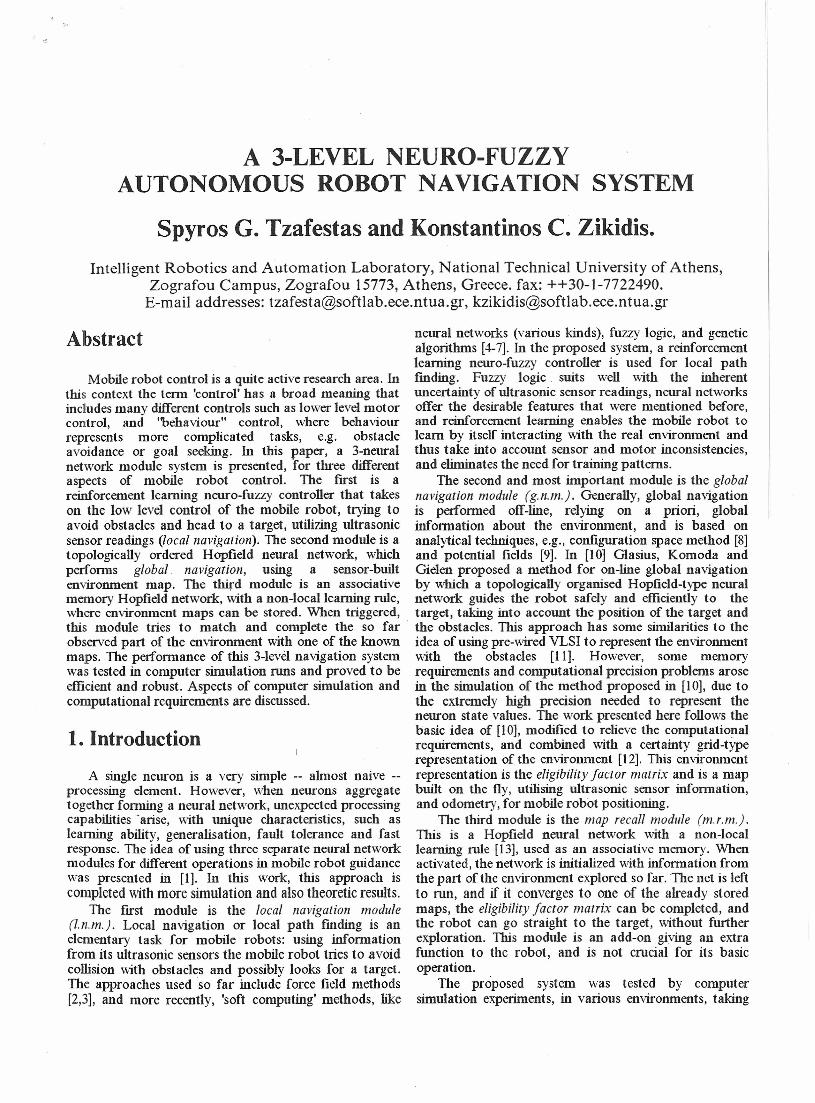
Figure 1: The robot-car and its sensor lobes and suit s,for forward and backward movement.
2. The robot model
The robot model used in the simulation is like a smallcar, 10 length units long and 3 units wide. The maximumangle of the steering wheels is ±45°. A positive anglecorresponds to a left tum. The controlling algorithm hascontrol over the steering angle, the direction of movement(forward-backward), and the speed to a lesser extend.
Ten ultrasonic sensors were used, with maximumrange 62 units and minimum range 4units. The lobes aresupposed to be 150wide. To simulate the ultrasonic wavelobe, 10 distance levels were used. Whenever one of thesensors reads the lowest distance level (4 units) the robothas approached an obstacle beyond a safety limit, and issupposed to have failed. The second distance level (8units) causes reversing of direction. If the robot movesforward and one of its sensors reads a second leveldistance, the robot starts moving backwards, and vice-versa. This is a simple way to overcome the limitedmaneuverability of a car-like robot, which cannot tum onthe spot. Motion is also reversed when the target islocated in the opposite direction of movement.
AlI sensors are used to build the map, thus exploitingthe maximum possible information. However, a kind ofpreprocessing is performed in the sensor readings forobstacle avoidance, in order to keep the number of thel.n.m. inputs low and discard unwanted information.Therefore, sensors form 'suits'; all sensors on the right sidegive one reading (the minimum value) and allleft sensorsgive their minimum. ln this way, only three distancereadings are fed to the obstacle avoidance algorithm: left,right, and front. Furthermore, high value readings (i.e.away) from the lateral sensors are ignored, since an
obstacle located to the side of the robot cannot be adanger. ln backward movement, the sensor suits are morecomplicated, since an obstacle located to the rear-left ofthe car requires the same maneuver as an obstacle locatedto the right, near the car: the steering wheels should tumto the right while the car is moving backwards. ln Figurel, one can see the 10full sensor lobes, as well as the sensorsuits for the forward movement (Left, Front, Right) , andalso for the backward movement (Left, Back, Right).
The speed is approximately 4 units per time step. It isreduced when the robot approaches obstacles, turnsabruptly, or moves backwards. This is the robot modelused in the present work, also used in [6]and [1].
3. The Local Navigation Module
As mentioned above, the l.n.m. is a neuro-fuzzycontroUer. The controlling algorithm is ASAFES2 [14],which is based on the Sugeno fuzzy reasoning method orfunctional reasoning [15].ASAFES2 assumes a partitionof the domain into a number of fuzzy sets, and tries toestablish a fuzzy rule in the form of a linear equation ineach subdomain, with the help of neural algorithms. Theoutput value is a weighted average of the output values ofeach activated fuzzy rule. The advantages of ASAFES2are fast learning, human-like reasoning, and goodperformance with few rules. On the other hand, the maindrawback is the curse of dimensionality: the complexity ofthe algorithm increases exponentially with the number ofinput variables. Also, in the form used in the presentstudy, it does not perform structure identification.
ln order to perform reinforcement learning, it is usedin an 'actor-critic' configuration [16]: the critic networktransforms the 'raw' feedback from the environment into amore informative, heuristic signal that is exploited by theactor network. ln this way, the controlling algorithmleams by a trial-and-error procedure, interacting directlywith the environment. The need for training patterns iseliminated and the specifie characteristics of the sensorsand actuators are taken into account.
This architecture is applied directly to mobile robotmotor control, using as inputs the (preprocessed) sensorreadings and the heading error, i.e. the angle required forthe robot to tum to head straight to the target, which issupposed to be given. The output is fed to the steeringmotor (properly scaled and limited to [-45°,+45°]).
The feedback from the environment is a single scalarand serves as an evaluation of the algorithm performance.ln many cases of reinforcement learning control tasks, thefeedback cannot be available before a series of actions hastaken place. For example, a feedback could be only afailure signal when the robot collides with an obstacle,and a success signal when the robot is away fromobstacles and is heading to the target. ln this case, thefeedback contains too little information, and thealgorithm would require extremely long training times todiscover and leam the desired behaviour. Thus, areinforcement signal is fed to the algorithm at the end ofevery time step, containing information that enables thealgorithm to discover quickly and acquire an obstacle
avoidance behaviour, and consequently a goal seekingbehaviour. A more analytic discussion of these issues canbe found in [6].
The l.n.m. is trained independently before being usedin the 3-levelnavigation system. If the heading error is setto zero, the robot simply wanders in the free space.
4. The Global Navigation ModuleThis module is a Hopfield neural network, with
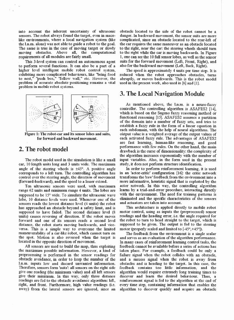
analog neurons, topologically ordered to represent theenvironment. ln every time step, the Hopfield network ofthe g.n.m. is mu and finally comes up with a virtual targetplaced near the robot. The heading error fed to the l.n.m.is caIculated with respect to this virtual target and not theactual target. ln this way the robot follows the virtualtarget, which eventually becomes the actual target (Figure2 depicts a similar biological system). Note that at everytime step a Hopfield net is initialised and mu, until itproduces a meaningful result. This might seem verycomplicated and time consuming, but simulation resultsindicate that it is not prohibitive; on the contrary it ismuch simpler and reliable than other analytic navigationtechniques.
localnavigation
module
globalnavigation
module
1
'\virtualtarget
Figure 2: The heading error fed to the local navigationmodule is calculated with respect to the virtual target
offered by the global navigation module.
The environment is represented on a lattice-likenetwork. ln the computer simulation, the environmentcovered a 640x380 square units area. To simplifycaIculations, al: 10 scale is used, and in tbis way the mapis represented by a rectangular grid of 64x38 analogneurons, whose states take values in [0,I]. The state valueof the neuron corresponding to the target position isalways set to unity. ln [10] the states of the neuronscorresponding to obstacles are clamped to the value ofzero. One can imagine a binary matrix with the size of theHopfield net (64x38), where Osrepresent obstacles and lsrepresent free space. At each Hopfield net iteration, thestate of each neuron is multiplied with the correspondingelement, and thus the states of the obstacle-neurons areset to 0, while the rest remain unaffected.
ln the present system, the environment map isconstructed on the way using the ultrasonic sensorreadings, assuming that the position and orientation ofthe mobile robot can be caIculated from dead reckoning.The information gathered by the sensors is not accurate,due to poor directionality, frequent misreadings andspecular reflections [2,3]. Therefore it is not wise to use abinary matrix to represent the environment. Hence, the
idea of the eligibility factor matrix was employed, allowingthe elements of the environment matrix to take real valuesin [0,1].The bigher the eligibility factor of an element, thehigher the probability that the corresponding area is freespace. Issues concerning the construction of the eligibilityfactor matrix (which is the environment map) will be dealtwith in the next section.
The number of neurons in the net is 64x38=2432. If amatrix representation is assumed also for the Hopfieldnetwork, then sij and eij are the state and the eligibility ofthe neuron located in the (i)th column and the G)th row.The weight connections are symmetric, excitatory(positive) and prohibit self-coupling. The importantditIerence from the ordinary Hopfield network is that theconnections are short ranged, allowing each neuron toreceive activation only from the eight neighbouring ones:neuron (i,j) receives activity only from neurons(i +k , j +1), k = -1,0,1,/ = -1,0,1, b:./. Connection weightsbetween neighbouring neurons are equal to one, and aIlother connections (including self coupling ones) are zero.
ln the case of discrete-time dynamics, the equationgiving the state of each neuron is:
s!i(t+l)=f[a·e.!i· :~>i+kj+/(t>I (1)k=-I,OJ/=-1,0,1Ikl+l~>O
where a is a parameter controlling the gain of the neuronsand f is a function. Updating the neuron states can takeplace in paraIlel, asynchronously (one at a time, atrandom), or sequentiaIly. Both parallei and sequentialupdating were tested. Even though the latter was the mostcomputationally effective, some problems wereencountered, and thus the parallel update was used.
......... ............................•...........................
11~~llliill:I:III: •••:iiw····~!:::::::·::II.I·I............. ,,, .:::::::::::::::::::::::::::" : ::'.::::::::........................... . ..•.................................... . .................................... ................................. .......................................................................................... . .................................. . ................................... . .................................................................................................................................................................::::::::::::::::::::::;:::::::::::::::::::::::::::::::::::::::
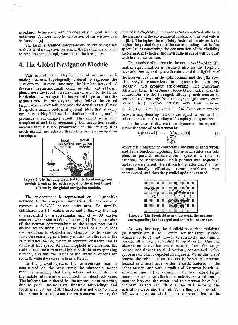
Figure 3: The Hopfield neural network: the neuronscorresponding to the target and the robot are shown.
At every time step, the Hopfield network is initialised(all neurons are set to 0, except for the target neuron,which is set to 1), and allowed to mu freely, updating inparallei all neurons, according to equation (1). One canobserve an 'activation wave' starting from the targetneuron and flowing to aIl directions, constrained in freespace areas. This is depicted in Figure 3. When tbis 'wave'reaches the robot neuron, the net is frozen. AlI neuronslocated in a small area (within a circle centered on therobot neuron, and with a radius of 3-neuron length, asshown in Figure 3) are examined. The next virtual targetneuron is the one with the higher activity provided that aIlneurons between the robot and this neuron have higheligibility factors (i.e. there is no wall between theactivation wave and the robot). ln tbis way, the robotfollows a direction which is an approximation of the
gradient. Moreover, the trajectory of the robot is smooth,and abrupt turns, that would be the result of assigningonly adjacent neurons as virtual targets, are avoided.This is repeated until the robot reaches the actual target.
According to [10], in a similar situation of a 2-dimensional environment where each neuron receivesactivity from its 8 neighbours, the parameter a must takevalues in [0,0.125), to guarantee stability and uniquenessof the equilibrium state. For the function f, the linear andthe tanh(x) function were tested. It is true that in the caseof the linear function, when a ~ 0.125 (=1/8), the networkis unstable and the neuron states take infinite values.However, if a bounded function is employed, the neuronscannot take inftnite values, even if a ~ 0.125.
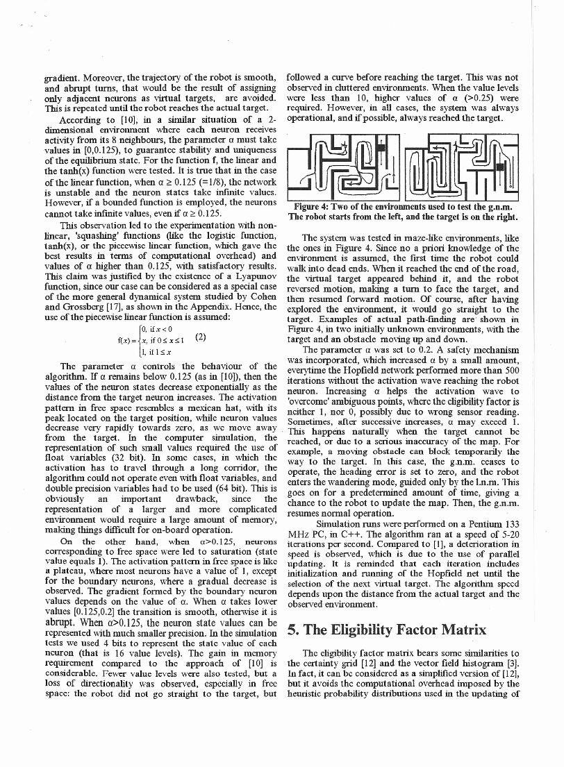
This observation led to the experimentation with non-linear, 'squashing, functions (like the logistic function, The system was tested in maze-like environments, liketanh(x), or the piecewise linear function, which gave the the ones in Figure 4. Since no a priori knowledge of thebest resuIts in terms of computational overhead) and environment is assumed, the first time the robot couldvalues of a higher than 0.125, with satisfactory results. walk into dead ends. When it reached the end of the road,This claim was justified by the existence of a Lyapunov the virtual target appeared behind it, and the robotfunction, since our case can be considered as a special case reversed motion, making a turn to face the target, andof the more general dynamical system studied by Cohen then resumed forward motion. Of course, after havingand Grossberg [17], as shown in the Appendix. Hence, the explored the environment, it would go straight to theuse of the piecewiselinear function is assumed: target. Examples of actual path-fmding are' shown in
10, if x < ° Figure 4, in two initially unknown environments, with the
f(x) = x, if 0:::; x s 1 (2) target and an obstacle moving up and down.The parameter a was set to 0.2. A safety mechanism
Lif l s » db Ilwas incorporated, which increase a y a sma amount,The parameter a controls the behaviour of the everytime the Hopfield network performed more than 500
algorithm. If a rernains below 0.125 (as in [10]),then the iterations without the activation wave reaching the robotvalues of the neuron states decrease exponentially as the neuron. Increasing a helps the activation wave todistance from the target neuron increases. The activation 'overcome' ambiguous points, where the eligibilityfactor ispattern in free space resembles a mexican hat, with its neither l, nor 0, possibly due to wrong sensor reading.peak located on the target position, while neuron values Sometimes, after successive increases, a may exceed 1.decrease very rapidly towards zero, as we move away . This happens naturally when the target cannot befrom the target. ln the computer simulation, the reached, or due to a serious inaccuracy of the map. Forrepresentation of such small values required the use of example, a moving obstacle can block temporarily thefloat variables (32 bit). ln sorne cases, in which the way to the target. ln this case, the g.n.m. ceases toactivation has to travel through a long corridor, the operate, the heading error is set to zero, and the robotalgorithm could not operate even with float variables, and enters the wandering mode, guided only by the l.n.m. Thisdouble precision variables had to be used (64 bit). This is goes on for a predetermined arnount of time, giving aobviously an important drawback, since the chance to the robot to update the map. Then, the g.n.m.representation of a larger and more complicated resumes normal operation.environment would require a large amount of memory, Simulation runs were performed on a Pentium 133making things difficult for on-board operation. MHz PC, in C++. The algorithm ran at a speed of 5-20
On the other hand, when a>O.125, neurons iterations per second. Compared to [1], a deterioration incorresponding to free space were led to saturation (state speed is observed, which is due to the use of parallelvalue equals 1). The activation pattern in free space is like updating. It is reminded that each iteration inc1udesa plateau, where most neurons have a value of l , except initialization and running of the Hopfteld net until thefor the boundary neurons, where a graduaI decrease is selection of the next virtual target. The algorithm speedobserved. The gradient formed by the boundary neuron depends upon the distance from the actual target and thevalues depends on the value of a. When a takes lower observed environment.values [0.125,0.2]the transition is smooth, otherwise it isabrupt. When a>O.125, the neuron state values can berepresented with much smaller precision. ln the simulationtests we used 4 bits to represent the state value of eachneuron (that is 16 value levels), The gain in memoryrequirement compared to the approach of [10] isconsiderable. Fewer value levels were also tested, but aloss of directionality was observed, especially in freespace: the robot did not go straight to the target, but
followed a curve before reaching the target. This was notobserved in cluttered environments. When the value levelswere less than 10, higher values of a (>0.25) wererequired. However, in aIl cases, the system was alwaysoperational, and ifpossible, always reached the target.
Figure 4: Two of the environments used to test the g.n.m.The robot starts from the left, and the target is on the right.
5. The Eligibility Factor MatrixThe eligibility factor matrix bears sorne similarities to
the certainty grid [12] and the vector fteld histogram [3].ln fact, it can be considered as a simplified version of [12],but it avoids the computational overhead imposed by theheuristic probability distributions used in the updating of

the certainty values of the cells (e1ements).ln the eligibility factor matrix approach, the elements
take values in [0.1]. A value of 1 corresponds to freespace, while 0 corresponds to an obstacle area. Initially,the whole environment is assumed to be free space. Atevery time step, all sensors are sampled. Suppose that asensor detects an obstacle in a distance of d length units.Uncertainty increases with distance. SOt let k = d/max d •where maxd is the maximum detection range of thesensors (in our case maxd=62). Then, the followingupdatings take place. on the eligibility factors of theelements lying on the acoustic axis of the sensor:
1. For all elements witbin a distance lower than d:eij=k.eij+(l-k)
2. For the e1ement in a distance equal to d: eij = k· eij
ln tbis way, the eligibility factor of elementscorresponding probably to free space (obstacle area) isincreased (decreased), by an amount depending on thedistance from the robot. ln order to keep the memoryrequirements low, the e1ements of the eligibility factormatrix were represented by 15 value levels (4 bits). The16th level indicates unseen area.
Since planning is based on building a map, anaccurate positioning technique is required. The proposedguidance system was tested on simulation only, where themobile robot position was accurate1y known, and wasassumed to be calculated with the use of dead reckoning.However it is well known that in the real world, deadreckoning leads to unbounded errors. ln other words,global navigation depends entirely on an efficient absolutepositioning technique.
6. The Map Recall ModuleThis is a separate ordinary Hopfield net used as an
associative memory, trying to recall and complete apartially observed environment. This net has also 64x38neurons, with a one-to-one correspondence to the neuronsof the g.n.m. net. The net in tbis module is represented bya vector v. whose e1ements vi' i= 1.2•...•2432. take thevalues {-1.0.+1}. -1 represents free space, +1 is obstaclearea, and 0 means 'don't know', and is used in theinitialization of the net to prevent unseen areas frombiasing the out come.
The simple Hebbian rule aImost always converged tospurious states [18]. because of correlations between thepatterns. A non-Iocalleaming rule was used [13], yie1dinga capacity of N patterns, where N is the number ofneurons. According to tbis rule, the weight matrix W issymmetric and probibits self coupling:
1 p p
if j;t J'. W.. = - "" I;~ .1;': . (çl) ,else Wii = 0'J N L,;L,;, J Il'
p.=1 ,'=1
Here ç~is the (i)th e1ement of the (fl)th training pattern, p
is the number of training patterns, and (C-1) is theinverse of the overlap matrix defmed by:
C~v = ~tc,,:'c,;1=1
The updating equation is:
Vi =sgnQ:::w. ,vj}j
where sgn(x) is the signum function.Each time the net was initialised, all neurons
corresponding to positions with eligibility factors bigherth an 0.5, were assigned a value of -1. while all neuronswith corresponding eligibility factors lower th an 0.5 wereassigned the value of +1. Neurons corresponding tounexplored areas were assigned the value of zero. ln ourcase the weight matrix is quite large. while the number ofpatterns is rather small (p=6). SOt instead of storing theweights, they were calculated each time they were needed.The sequential updating was preferred.
The time required for a complete iteration of thenet (i.e., for updating all neurons) was less than 1.5minute. on the same computer. The net showed excellentperformance and converged always to the right pattern.most times in a single iteration. after observing only asmall fraction of the environment. The recalled pattern isused to correct and complete the eligibility factor matrix.
7. ConclusionA 3-module navigation system was presented. AIl
modules were implemented by neural network structures.A reinforcement neuro-fuzzy controller was used for localnavigation acquiring an obstacle avoidance and goalseeking behaviour via a trial and error procedure. Atopologically organised Hopfie1d net was the core of theglobal navigation module, yie1ding excellent results in allsituations. Finally, a usual Hopfield net was used as anassociative memory able to store a large number of mapsand recall a map, even when only a small fraction has
. been observed. The computer simulation results were veryencouraging.
8. AppendixAccording to [17] a global Liapunov function can be
defmed for N-dimensional competitive dynamical systemsthat can be written in the form:
N
x; = a;(xJ[h;(xJ- LCDe ·dk(xdJ. i=I.2 •...•N. (3)k=1
where the coefficients cij form a symmetric matrix,
a.(x.)~O, and ~d(xd~O. i.e. the function d(x) is1 1 dX
k
monotone. This Liapunov function is:N JX 1 N
V(x) = -L' b;(ç)d;(ç)d{ + - LC,kdj(Xj)ddXk);=1 0 2 j,k=1
Our case belongs to tbis category as shown be1ow.ln the equations that follow, the values of the neuron
states are not represented in matrix form (sif)' as was thecase in equation (1), but in vector notation. So, theneuron state values are represented as s il i= 1•...•N. whereN is the number of neurons (in our case 64x38=2432).H'Zowever, the notion of "neighbourhood" pertains to the
matrix representation of neurons. Let:N
xj(t) = L wif 'Sj(l) = LSj (1)j=l neighbouring
neurons
where W Ii is the connection weight from neuron (i) toneuron (j). Note that these connection weights aresymmetric, excitat ory , and short range. Namely:W if = W jj = 1 ifI neurons (i) and (j) are neighbours and i:;tj,
otherwise wif = O. Therefore, the state of each neuron,which equals the summation of the state values multipliedby the respective connection weights, over the whole set ofneurons, is reduced to adding the state values of theneighbouring neurons. Consider equation (1) without theeligibility factor ejj, with vector notation:
sj(t+l)=f[a· LSj{t»)=:>neighbouring
neurons
d ~~-Sj(t) = Sj(l+I)-Sj(l) =f[a· LSj(t»)-Sj(t) <=>dl neighbouring
neurons
.!!..-Sj(t) = f[a·xj(t»-Sj(t)dt
Summing up over the whole set of neurons andmultiplying by the corresponding weights yields:
N d N N
~!Vif' dt Sj(t) = ~ wij ·f[a,xj(t» - ~ w!i''Sj(t) <=>
d N N
dt ~ wij 'Sj(t) = ~ wij ·f[a,xj(t»- xj(t) <=>
d N-xj(t) = L wif .f[a,xj(t»)- x/t)dt j=l .
Setting aj(xj) = +1, h;(xj) = -Xj' dj(x) = f(a·x), andcij = -wij' equation (3) becomes:
d N-x· = "w ... f(a·x.).-x.dt 1 L... y } 1
j=l
which is equation (6), with the time parameter suppressed.ln the above syllogism, the parameter a did not play
any role. Consequently, the global stability of the systemdescribed by equation (1) does not depend on the valuesof this parameter, as long as the values of the neuronstates remain bounded. Since the non-linear function f(x)is bounded, the proposed system is globally stable. Thesystem proposed in [10] has to satisfy the conditiona<0.125, because otherwise, in the case of the linear(unbounded) neuron output function, it does not satisfythe elementary eriterion of BIBO stability: a boundedstimulation from the target neuron yields inftnite neuronstate values.
9. References[1] S. G. Tzafestas and K. C. Zikidis, "A mobile robotguidance system based on three neural network modules",in Proc. of 2nd ECPD Con! on A dv. Robotics, Intell.Autom. and Active Systems, Vien na, Austria (1996).[2] J. Borenstein and Y. Koren, "Real-time obstacleavoidance for fast mobile robot", IEEE Trans. Syst.,
Man, Cyber., 19,no.5,pp. 1179-1187(1989).[3] J. Borenstein and Y. Koren, "The Vector FieldHistogram - Fast obstacle avoidance for mobile robots",IEEE Journal of Robotics and Automation, 7, no. 3, pp.278-288 (1991).[4] R. Bielwald, "A neural network controller for thenavigation and obstacle avoidance of a mobile robot", inNeural Networks for Robotic Control, A.M.S. Zalzala andA.S. Morris, eds., Ellis Horwood, Hertfordshire UK 1996.[5] H. R. Beom and H. S. Cho, "A sensor-basednavigation for a mobile robot", IEEE Trans. Syst., Mail,Cyber., 25, no.3, pp: 464-477 (1995).[6] S.G. Tzafestas, K.C. Zikidis and G.B. Stamou, "Areinforcement learning fuzzy logic controller for themobile robot local path finding problem", in Proc. Intl.Symposium on Soft Computing, Reading UK (1996).[7] IEEE Trans. Syst., Man, Cyber., 26, no. 3 (Specialissue on learning autonomous robots, June 1996).[8] T. Lozano-perez and M. A. Wesley, "An algorithm forplanning collision-free paths among the polyhedral
(5) obstacles", Communications of the A CM, 22, no. 10,pp.560-570 (1979).[9] O. Khatib, "Real-time obstacle avoidance formanipulators and mobile robots", Int. 1. of RoboticsResearch, 5, no. l, pp. 90-98 (1986).[10] R. Glasius, A. Komoda and S.C.A.M. Gielen,"Neural network dynatnics for path planning and obstacleavoidance", Neural Networks, 8, no.I, pp.125-133 (1995).[Il] L. Tarassenko, M. Brownlow, G. Marshall, J. Tombsand A. Murray, "Real-time autonomous navigation usingVLSI neural networks", in Adv. in Neural ln! Proc. Syst.3, R. P. Lippmann, J. E. Moody and D. S. Touretzky,Eds., Morgan Kaufmann, San Mateo, CA (1990).[12] A Elfes, "Sonar-based real-world mapping andnavigation", IEEE J. of Robotics and Autom., RA-3, no.3,pp. 249-265 (1987).[13] I. Kanter and H Sompolinsky, "Associative recall ofmemory without errors", Physical Review A 35, no. l ,pp.380-392 (1987).[14] K.C. Zikidis and A.V. Vasilakos, "A.S.AF.ES.2: anovel, neuro-fuzzy architecture for fuzzy computing,based on functional reasoning", Fuzzy Sets and Systems83 pp.63-84 (1996).[15] T. Takagi and M. Sugeno, "Fuzzy identification ofsystems and its application to modeling and control",IEEE Trans Syst., Man, Cybern., 15, pp. 116-132 (1985).[16] AG. Barto, R.S. Sutton, and C.W. Anderson,''Neuronlike adaptive elements that can solve difficultlearning control problems", IEEE Trans Syst., Man,Cybern., 13, no. 5, pp.834-846 (1983).[17] M. A. Cohen and S. Grossberg, "Absolute stability ofglobal pattern formation and parallel memory storage bycompetitive neural networks", IEEE Trans. on Syst., Mailand Cybern. 13, no.5, pp. 815-826 (1983).[18] S. Haykin, ''Neural networks, a comprehensivefoundation", Macmillan College Publ, Comp., NY (1994).
(4)
(6)