Autonomous Onboard Guidance and Navigation Performance ...

Autonomous Onboard Guidance and Navigation Performancefor Earth to Mars Transfer Missions

by

Peter J. Neirinckx

S.B., Massachusetts Institute of Technology (1990)

Submitted to the Department of Aeronautics and Astronauticsin partial fulfillment of the requirements for the degree of

Master of Science in Aeronautics and Astronautics

at the

MASSACHUSETTS INSTITUTE OF TECHNOLOGY

January 1992

@ Peter J. Neirinckx, 1992. All rights reserved.

Author ........ .................................. 4.... ... ....Department of Aeronautics and Astronautics

January 16, 1992

Certified by .............................................:. ..........,..-....... ..Professor Richard H. Battin

Adjunct Professor. of Aeronautics and AstronauticsThesis Supervisor

Certified by...............

Certified by................

Principal Member,

Kenneth M. SpratlinGroup Leader, The Charles Stark Draper Laboratory, Inc.

Technical Supervisor

.... .......... Y z..- Iey........ ... .Sfanley W. Shepperd

Technical Staff, The Charles Stark Draper Laboratory, Inc.Technical Supervisor

Accepted by ............................ ............ ... ........ ............. ......SProfessor Harold Y. Wachman

MAs4 ':Fs ~u'ma Chairman, Departmental Graduate Committee

,F ~ 0 1992

I ýý -r - . - -• '•-''•- .•..

UiBRAki6S

Autonomous Onboard Guidance and Navigation Performance

for Earth to Mars Transfer Missions

by

Peter J. Neirinckx

Submitted to the Department of Aeronautics and Astronauticson January 16, 1992, in partial fulfillment of the requirements

for the degree ofMaster of Science in Aeronautics and Astronautics

Abstract

In preparation for manned missions to Mars, autonomous onboard guidance and nav-igation is studied as a backup to ground-based navigation systems. A survey of theliterature indicates that autonomous interplanetary navigation is viable and desirable.However, due to the reliability and accuracy of ground-based methods, little has beendone in this area. for the past two decades. Since that time, the accuracy and reliabilityof onboard navigation instruments have improved significantly. A refinement of the olderstudies is performed by developing an interplanetary autonomous navigation and guid-ance (AG&N) computer simulation. A linear error covariance analysis provides the basisfor the simulation, and an Earth to Mars Hohmann transfer mission defines the base-line interplanetary trajectory. The development is extensively detailed, and citations areprovided to promote future reference.

The interplanetary simulation is coupled to an existing Mars approach computer simula-tion [Shepperd, S. W., et al, Onboard Preaerocapture Navigation Performance at lMars,AAS Paper 91-119, 1991]. Both the interplanetary and approach performances for asample Mars a.eroca.pture mission are examined based on several convenient figures-of-merit. It is found that the mission can be performed successfully using only AG&Nduring the entire mission. A parameter sensitivity analysis is also performed, resultingin a more comprehensive understanding of the AG&N problem. Further investigationsare suggested.

Thesis Supervisor: Professor Richard H. BattinTitle: Adjunct Professor of Aeronautics and Astronautics

Technical Supervisor: Kenneth M. SpratlinTitle: Group Leader, The Charles Stark Draper Laboratory, Inc.

Technical Supervisor: Stanley W. ShepperdTitle: Principal Member, Technical Staff, The Charles Stark Draper Laboratory, Inc.

Acknowledgments

I am truly grateful to CSDL for the opportunity to have pursued my studies at MIT

and to have gained so much experience in the astrodynamics field. I would like to thank

Professor Dick Battin for his inspirational teaching. Space exploration continues in the

world today in part because of the excitement Professor Battin fosters. I would like

to recognize and thank Stan Shepperd for his support, patience, and insightful guidance

throughout the past months. Ken Spratlin and Tim Brand deserve many thanks for their

helpful directions and the original thesis concept. Much appreciation is also conveyed to

Wayne McClain for his initial help at CSDL and for his encouragement of further pursuits.

To my mother and father, I would like to especially express my gratitude. Their con-

tinued love and devotion I deeply cherish. They, along with Sandra, John, and Cheryl,

are my foundation. To all the friends along the way who have shared of themselves and

have lent an ear: thank you Anthony, Catherine, Cindy, Dennis, Kate, Steve, Susan and

many more!

I would like to dedicate this thesis to my grandfathers, Wilmer Kenney and Edward

Neirinckx.

This report was prepared at The Charles Stark Draper Laboratory, Inc. under NASA

Contract NAS9-18426. Publication of this report does not constitute approval by the

Draper Laboratory or the sponsoring agency of the findings or conclusions contained

herein. It is published for the exchange and stimulation of ideas.

I hereby assign my copyright of this thesis to The Charles Stark Draper Laboratory,

Inc., Cambridge, Massachusetts.

Peter Joseph Neirinckx

Permission is hereby granted by The Charles Stark Draper Laboratory, Inc., to the

Massachusetts Institute of Technology to reproduce any or all of this thesis.

List of Acronyms and Symbols

Note: A bold-face, lower-case symbol indicates a vector quantity while a bold-face, upper-

case symbol indicates a matrix quantity. The magnitude or trace of the symbol is indi-

cated by normal-face text.

Symbol Description

AG&N autonomous (interplanetary) guidance and navigationDSN Deep Space NetworkECRV exponentially correlated random variableEI entry interface (atmosphere at 125 kilometers above Martian surface)FOM figure-of-meritFOV field-of-viewfps feet per secondGPS Global Positioning Systemhrs hoursIMU inertial measurement unitKF Kalman filterLOS line-of-sight (generally to Mars), LOS coordinate system (with x = LOS

direction and z = angular momentum direction of the s/c trajectory)LVLH local vertical / local horizontal coordinate system (with y = radial

direction and z = trajectory angular momentum direction)m/s meters per secondOD orbit determinationPN process noiserms root mean squarels•c arcsecondss/c spacecraftSOI sphere of influence at MarsTCM Trajectory Correction Maneuverwrt with respect to

a semi-major axis (of trajectory or error ellipsoid)b semi-minor axis (of error ellipsoid); bias percentageB linear guidance matrixe state uncertainty vector, eccentricity vectorE state covariance matrixDD velocity correction uncertainty matrixDV velocity correction matrixAv state uncertainty vectorh periapse altitude; angular momentum magnitudeh measurement sensitivity vector; angular momentum vector

i

IkAMN

Qrlo

t

xEx

XZ

orbit inclinationidentity matrix of appropriate dimensionKalman gain vectoraerocapture FOMcompatibility matrixintegrated process noise matrixgravitational constant (solar or Martian); microangle between error ellipsoid semi-major axis and(linear) state transition matrixprocess noise matrixinertial position vectorstandard deviation (or 3o), equal to (three times)

quantities with zero mean valuestimeunit vectorinertial velocity vectorstate vectoractual state error vectorestimated state error vector6 x 6 mean squared actual error matrix, position and velocity6 x 6 position and velocity error correlation matrix (actual to estimated)

Subscripts

actE

fIhIImneas71077n

ppolerefrel

Superscripts

Description

actualellipticalfinal (nominal SOI or periapse)angular momentumhyperbolicmeasurednominalperiapseMars rotational axisreference value, nominalMars relative

Description

degrees

value immediately after a measurement or TCMfirst total time derivativesecond total time derivativethird total time derivativetranspose

defined x axis

the rms value for

List of Figures

2-1 The State Uncertainty Vector ...... .. . .. .............. . 11

2-2 Relative Geometry for the Optical Measurement ............... 27

2-3 Example Star Tracker Pixel Array ................... ... 28

2-4 Geometry of the Same-Plane Centroid Bias .................. 29

3-1 Minimizing the Cost of VTOA Guidance ................... 44

3-2 The Compensation Vector for VTOA Guidance ............... 45

3-3 Plot of Equation 3.37 ............................. 47

3-4 Periapse Altitude Sensitivity to State Errors in a Mars LOS Coordinates 47

4-1 The Baseline Hohmann Trajectory ....................... 58

4-2 Geometry of the Deimos sightings ................... ... .. 60

4-3 Linear Approximation to Obtain the Process Noise Velocity Components 63

4-4 Simulation Flowchart ............................. 66

4-5 Aerocapture Accuracy Requirements (1) at Entry Interface ........ 67

4-6 Aerocapture Accuracy Requirements (2) at Entry Interface ........ 68

4-7 Cartoon of a 1 SOL Orbit .......................... 68

4-8 Current Position Uncertainties in Mars LOS Coordinates ......... . . 70

4-9 Current Position Uncertainties in LVLH Coordinates. ......... . 70

4-10 LOS and LVLII Coordinate Definitions .................... 71

4-11 Position Uncertainties in LVLH Coordinates: No Navigation ....... 71

4-12 Planetary Distances and LOS Rates for the Hohmann Transfer. ...... . 73

4-13 Final Approach for the Hohmann Transfer ............... . . . 73

4-14 Optical Angular Diameters of the Planets .................. 7.5

4-15 Optical Angular Diameters of the Mars System ............... . . 75

4-16 SOI Position Uncertainties in Mars LOS coordinates ............ . . 76

4-17 Position Error Ellipsoid Cross-Section in the Mars LOS Frame ....... .76

4-18 Position Error Ellipsoids at the SOI, at EI, and at Periapse ........ .. 77

4-19 Effect of Dynamics on Errors With No Navigation During Mars Approach 77

4-20 Periapse Altitude and Inclination Uncertainties ............... .78

4-21 SOI Position Uncertainties in Mars LOS coordinates: Baseline simulation

without course corrections .......................... 79

4-22 Current RMS Velocity Uncertainties in Mars LVLH Coordinates ..... . 79

4-23 SOI Velocity Uncertainties in Mars LVLH Coordinates ........... 81

4-24 Periapse Altitude and Inclination Dispersions Showing FTOA Targeting

Accuracy ........... ...... ................... 81

4-25 FTOA Cost to Correct for LOS Errors ................... 82

4-26 Baseline Performance for Three Cases of the Approach Simulation . . . . 84

4-27 Baseline Performance for The Optical Case of the Approach Simulation . 85

4-28 Relative Geometry of the Error Ellipsoid for Approach Navigation . . . . 85

5-1 Approach Navigation Figures-of-Merit for Variational Case 2 ........ 93

5-2 LOS Position Uncertainties for Variational Case 3 .............. 94

5-3 LVLH Velocity Uncertainties for Variational Case 3 ............. 94

5-4 Approach Navigation Figures-of-Merit for Variational Case 7 ....... 96

5-5 Mars Observer Trajectory: x-y planar projections .............. 100

5-6 Sprint Trajectory: x-y Planar Projections ................... 101

5-7 Approach Navigation Figures-of-Merit for Variational Case 12 ...... 101

5-8 Earth-LOS Current Position Uncertainties: Doppler tracking of Earth

without optical measurements ...................... .. 103

5-9 Earth-LOS Current Position Uncertainties: Range tracking of Earth with-

out optical measurements .......................... 104

5-10 Approach Navigation Figures-of-Merit for Variational Case 16 ...... 106

6-1 Monte Carlo Simulations Varying a Four TCM Schedule .......... 112

D-1 Coordinate System for Minimizing the Velocity Correction ......... 127

D-2 Solution for the Optimal Velocity Correction ................. 128

E-1 LOS Position Uncertainties for a Case with No Earth Measurements . .. 134

E-2 LOS Velocity Uncertainties for a Case with No Earth Measurements . . . 134

List of Tables

4.1 Two-Body Initial Conditions For The Baseline Mission ........... 59

4.2 A Priori Error Covariance (Eo) Diagonals .................... 62

4.3 The Effects of Time Step on the Process Noise Integral (N) Approximation 64

4.4 Components of the Baseline Scenario .................... 65

4.5 Course Corrections for the Baseline Run ................... 80

4.6 Inertial Error Covariance and State for Mars Approach Hand-Over .... 83

5.1 Performance for Variations About the Baseline Scenario at the SOI, EI,and Periapse (Part 1) ............................. 88

5.2 Performance for Variations About the Baseline Scenario at the SOI, EI,and Periapse (Part 2) .................. .......... 89

5.3 Description of Objectives for the Variational Cases ............. 90

5.4 Approach Navigation Performance for Four Variational Cases ....... 91

5.5 Initial Conditions for the Mars Observer Variation: Inertial Coordinates. 99

5.6 Initial Conditions for the Sprint Orbit Variation: Inertial Coordinates... 100

E.1 List of Variations About Case 9 ................ ....... 133

E.2 List of Variations About Case 9, No Consider or Guidance States . . . . 133

Contents

1 Introduction

1.1 Background and Motivation . . . . .

1.2 Performance Analysis Objectives . .

1.3 Method and Assumptions . . . . . .

1.4 Thesis Overview.............

2 Navigation Theory

2.1 Choice of State Variables . . . . . . .

2.2 Linear Filter Development . . . . . .

2.2.1 Consider States . . . .....

2.3 State Propagation............

2.3.1 Position and Velocity States .

2.3.2 Bias States ..........

2.3.3 Propagation of the Covariance

2.3.4 Process Noise .........

2.3.5 Performance Parameters . . .

2.4 Observation Models...........

2.4.1 Optical Measurements . . . .

2.4.2 Radiometric Measurements. .

2.4.3 Optimum Measurement Selecti,

2.5 Navigation Instrument Errors . .

. . . . . . . . . .

. . . . . . . . . ...........

..........

. . . . . . . . . .

..........

Matrix. . . . . . ...........

. . . . . . . . . .Matrix ......

. . . . . . . . . .. . . . . . . . . .

on & Scheduling

. . . . . . . . . .

3 Guidance Theory

3.1 Impulsive Assumption ............................

3.2 Fixed Time-of-Arrival Guidance .......................

3.2.1 The Dispersion Matrix ........................

35

36

36

39

3.2.2 Potential Guidance Accuracy . . .

3.3 Variable Time-of-Arrival Guidance . . . .

3.4 Periapse Altitude and Inclination Guidance

3.4.1 Periapse Only ............

3.4.2 Periapse and Inclination . . . . . .

3.5 Burn Execution Errors . . . . . . . . . . .

3.5.1 Known and Unknown Errors . . . .

3.5.2 Three Models ............

3.6 Course Correction Scheduling . . . . . . .

4 Typical System Performance

4.1 Baseline Mission ....................

4.1.1 The Nominal Trajectory ............

4.1.2 Navigational Design ..............

4.1.3 Guidance Design ................

4.1.4 Summary ....................

4.2 Navigation Performance Requirements . . . . . . . .

4.3 Simulation Results & Analysis . . . . . . . . . . . . .

4.3.1 Interplanetary Navigation . . . . . . . . . . .

4.3.2 Mars Approach Navigation . . . . . . . . . . .

4.3.3 Summ ary ....................

5 Variational System Performance and Sensitivity

5.1 Navigational Sensitivities to Error Sources . . . .

5.1.1 Mechanical Error Sources . . . . . . . . .

5.1.2 Environmental and Filter Error Sources ..

5.2 Sensitivities to the Environment . . . . . . . . . .

5.2.1 Modified Measurement Schedule . . . . . .

5.2.2 Alternate Mission Trajectory . . . . . . . .

5.2.3 Inclusion of Radiometric Data . . . . . . .

5.2.4 Backup System Role ............

5.3 Guidance Sensitivities . . . . . . . . . . . . . . .

5.3.1 Mechanical Error Sources . . . . . . . . .

5.3.2 Alternate Guidance Scheme . . . . . . . .

Analysis

. . . 0 0

. . . 0. ° ,

..... o

87

92

92

95

95

95

98

102

102

104

105

105

5.3.3 Modified Correction Schedule .................... 107

6 Conclusions 109

6.1 General Summary ................... ............ 109

6.2 Summary of Sensitivity Results . . . . . . . . . . . . . . . . . . . . . . . 110

6.3 Future Research ................................ 111

Bibliography 113

A Extensions to Process Noise Derivation 117

B Alternate Guidance Methods 120

C Time of Periapse Passage Sensitivity 124

D Nominal Orbit Construction 125

E Variations on Earth Measurements 131

Chapter 1

Introduction

The United States has recently expressed a renewed interest in sending a human crew to

the planet Mars. As with the Apollo moon missions, the concern for crew autonomy has

surfaced. Especially in the event of problems, it may be desirable for the spacecraft (s/c)

to have the ability to perform navigation or trajectory maneuvers not under ground-

based mission control. An onboard interplanetary autonomous guidance and navigation

(AG&N) system is required to accomplish this goal. An autonomous system is one in

which all navigational measurements and calculations are performed using instruments

onboard the s/c; guidance is by definition an onboard problem'. Because of power

limitations, only optical measurements of stars and other heavenly bodies generally fit the

autonomous description. Other data types such as 1-way radiometric measurements can

also be considered as supplemental, though not truly autonomous. This thesis presents

a detailed AG&N system description and performance analysis in order to determine the

feasibility of such a system when applied to a Mars mission.

1.1 Background and Motivation

The concept of interplanetary AG&N is not new. Numerous studies have been conducted

beginning in the early 1960's to explore AG&N capabilities [2], [6], [17], [26], [40]. Indeed,

the concept has been demonstrated to some extent by the Mariner '71 mission [10].

Recent surveys of earth-orbiting AG&N capabilities were made in 1983 [12], 1984 [5],

1 A guidance capability acts through the propulsion system which is a physical component of thespacecraft.

and 1985 [27]. This thesis brings together many of the techniques and results from those

reports. Several sources will be cited often and are considered complementary reading.

The studies are by Cicolani et al. [6], [40], and Shepperd, et al. [33]. Battin's textbook [3]

is also a useful source.

The number of interplanetary AG&N studies, however, began to decline in the early

seventies2 . The Deep Space Network (DSN) began to provide ground-based tracking for

the infrequent unmanned interplanetary missions. The DSN worked (and still performs)

very well, providing excellent coverage, reliability, and most importantly, accuracy. As a

result, few studies have applied current autonomous instrument accuracies to the inter-

planetary navigation problem. This thesis intends to show that with these new instru-

ments, autonomous navigation provides adequate performance support for interplanetary

navigation and guidance. In particular, the interplanetary mission studied in this the-

sis is one in which the capture into Mars orbit is accomplished through an aerocapture

maneuver instead of propulsive capture. Since aerocapture imposes tighter guidance and

navigation accuracy requirements, less restrictive missions are assumed to be adequately

supported if a similar aerocapture mission can be supported.

Guidance mechanisms and accuracies have also improved over the past twenty years.

The coupling between interplanetary guidance and navigation performance becomes an

important issue when considering that the interplanetary spacecraft may be large, re-

quiring long burns with active control. This thesis addresses this issue by means of a

dispersion analysis.

The primary motives for studying the interplanetary AG&N problem are to update

the general knowledge of AG&N capabilities and to consider the possibility of a backup

system to the DSN. Other motivations exist and are briefly described below.

Motivation Summary and Problem Statement

This thesis is motivated by the presence of the following possibilities:

* Especially for a manned mission, a backup AG&N system is always desirable. Au-

tonomous navigation could be used to supplement the DSN, act as a system backup,

or replace it entirely in certain cases.

2 Distinguished from Earth-bound AG&N where numerous studies have been performed, especially inthe 1980's with the advent of the Global Positioning System.

* Previous studies have made certain approximations due to computational consid-

erations. In order to keep the problem simple, some AG&N covariance studies

did not include process noise or estimated only a small number of states. Current

computational facilities can support more complex analysis.

* On-board navigation instrumentation accuracies have improved since the last stud-

ies. Also, the interplanetary mission objectives and requirements have changed

significantly (i. e. can an AG&N system provide accuracies sufficient to support

aerocapture?). The former studies do not indicate a capability to handle the new

requirements. Verification of mission support with current capabilities is needed.

* The DSN is expensive to operate [12]. If a reliable cost-effective alternative system

with comparable performance exists, it should be investigated.

* The ability of a s/c to maneuver autonomously in interplanetary space could also

facilitate new applications. Specifically, future missions may involve multiple s/c

in flight at one time which ground-based systems may not be able to efficiently

support. Furthermore, small (robotic) spacecraft that could fly safely under their

own control, temporarily or continuously, would be a step toward the increased

exploration of the solar system.

1.2 Performance Analysis Objectives

Given the above motivation for autonomous navigation of interplanetary spacecraft, the

focus logically switches to answering the following question:

Problem Statement: "Can present-day autonomous guidance and navigation instru-

mentation provide sufficient interplanetary trajectory accuracy for a successful aerocap-

ture mission?"

A study by Shepperd, et al.[33] has previously analyzed the autonomous Mars ap-

proach (approximately two days prior to Mars atmosphere entry interface) navigation

problem, with interplanetary navigation provided by the DSN. This thesis essentially

extends the autonomous approach performance analysis to the interplanetary Earth to

Mars trajectory in an attempt to answer the Problem Statement and demonstrate the

current capabilities of AG&N for general interplanetary missions.

Also, by interpreting the Problem Statement as a feasibility philosophy, a baseline

mission should be chosen such that if the requirements are not met for that mission, it can

then be assumed that the requirements cannot be met for other missions. A secondary

objective of the study is to provide some insight into the system performance through

trajectory dynamics, geometry variations, and guidance/navigation interaction.

1.3 Method and Assumptions

An AG&N simulator has been developed in the HAL/S programming language on an

IBM 3090 mainframe computer at The Charles Stark Draper Laboratory, Inc. The simu-

lation and baseline mission constitutes various assumptions about the guidance hardware,

navigation instrumentation, and their inherent accuracies. The baseline autonomous nav-

igation is accomplished only through optical measurements. The computer simulation

performs a linear covariance analysis on the associated guidance and navigation errors.

As such, the analysis is only valid when the linearity assumptions are justified. The

output of such a simulation is a statistical representation of the performance that can be

expected from any mission similar to the nominal baseline mission.

For a successful mission, it is generally desired that the spacecraft position and veloc-

ity errors be kept small in order to keep the fuel and structure costs down. The ability

to maintain or sustain small errors is the purpose of navigation and the goal of guidance.

The definition of "small" is somewhat ambiguous, but generally means that if the Tay-

lor series of a function is taken, the quadratic and higher order terms can be neglected

since they are much "smaller" than the linear term. This "linearization" assumption is

paramount in this thesis. Linearization makes the effects of deviating from the nominal3

trajectory transparent. In other words, "error" terms evaluated off the nominal, but at

the same time, tend to have similarly valued derivatives. This effect is useful when trying

to get a qualitative feel for the effectiveness of AG&N for different missions.

To make a linear assumption, some knowledge of both the error type and the error's

functional relationships with desired quantities are needed. The particular types of errors

from navigational inaccuracies, guidance inaccuracies, and elsewhere are diverse but do

share an important characteristic. These error sources are generally stochastic in na-

ture and can be modeled as having Gaussian distributed values with zero means. Since

3 The constant portion of the function's Taylor series.

the desired quantities such as terminal miss uncertainty have been linearized about the

nominal, they are linear combinations of the state error variables. The desired quantities

are then Gaussian as well, and the AG&N analysis need only consider the covariances of

the quantities of interest to get a complete statistical description of the desired parame-

ters. A covariance analysis is then the appropriate methodological tool for this study. In

particular, the standard Kalman Filter (KF) has been chosen to optimally incorporate

the navigational measurements. The guidance equations are also incorporated into this

formulation. Though a deterministic Monte Carlo study can obtain similar results, that

method is very inefficient because of the large number of computer simulations required.

In contrast, the structure for this study is a linear error covariance analysis which requires

only a single run.

Below is a brief list of the assumptions made in this thesis. The list is intended

to enable the reader to interpret the derivations and results in the following chapters

appropriately and to formulate future work concisely.

Major Assumptions

* As with most other referenced studies, movement of the s/c with respect to (wrt) the

Sun and planets will be governed by two-body (conic) dynamics. The planets' orbits

are also conic. In addition, a patched-conic technique is used to propagate through

the Mars sphere-of-influence (SOI), itself another mathematical approximation.

* Any equations describing various error quantities will be linearized about the nomi-

nal mission trajectory by assuming the errors are small with respect to the nominal

value but much larger than the second-order terms.

* Navigational measurements that require stellar direction vectors will use ficticious

stars conveniently located. It is believed that the added complexity of adding a

star catalog to the simulation is unnecessary. A sufficient number of adequate

magnitude real stars can be found near a strategically placed ficticious star. Being

near the ficticious star means that the first-order navigation sensitivity to star

position should be the same. In other words, the information derived from either

real or ficticious star is essentially identical.

* Trajectory Correction Maneuvers (TCM's) are applied impulsively. It is important

to distinguish between correction maneuvers and rocket firings that exist as part of

the precomputed nominal path (e. g. plane change maneuvers or injection burns).

Some missions require some form of continuous thrusting or multiple impulsive

thrusts4 as part of the nominal path so that the target can be reached in a timeshorter than a free-fall path5. The nominal trajectories of this study avoid using

any maneuvers as part of the reference trajectory.

* Error sources are modeled as either white noise or exponentially correlated random

variables (ECRV). Their statistics will be given in later sections.

1.4 Thesis Overview

This thesis simulates an AG&N system to analyze its performance capabilities. Chap-

ters 1, 2, and 3 draw from the various cited works to describe the nominal mission and

develop the simulator. The detail of these chapters is such that the they are also intended

to serve as a guide for future linear covariance studies. Chapter 4 applies the simulator

to a baseline mission in order to show the feasibility of AG&N. Chapter 5 then performs

a sensitivity analysis on the system in order to determine the critical assumptions made

and their characteristic effect(s) on the AG&N system performance. Chapter 6 summa-

rizes the major points of this thesis and provides suggestions for further study. Lastly,

there are five appendices which elaborate on various topics from the main text.

4It is possible for a single injection burn to result in a sprint trajectory, but it would be very costly.SAn orbit that requires an impulsive injection burn.

Chapter 2

Navigation Theory

The purpose of navigation is to take measurements of the surrounding environment in

order to improve the current knowledge of the vehicle state (position and velocity). Due

to the presence of random errors in the measurements, only an approximate knowledge

can be obtained. However, the use of an optimal filter to incorporate the measurement

information minimizes the error in the knowledge of the state. This chapter discusses the

particular quantities to be estimated, the choice of filter, processing of measurements,

and the error sources modeled in the linear covariance simulator developed for this thesis.

2.1 Choice of State Variables

This section describes those key state parameters that are to be included in the estimation

process. In theory, all the variables and parameters of the problem are random variables

and should be estimated since, in fact, every "constant" physical quantity has been

measured' and is subject to random measurement errors. Additionally, the errors in the

random values are generally modeled as Gaussian with a zero mean value. Thus, all

biases in the variables and parameters must also be estimated by the filter. In order

to keep the problem tractable, only those quantities that are essential to the study of

navigation performance are included in the generalized state vector, x.

An important aerocapture performance parameter, or figure-of-merit (FOM), is the

periapse altitude, hp, of the s/c at the target planet (see [331). This and other performance

parameters can be derived from knowledge of the s/c position and velocity vectors, r and

1With finite resolution.

v, and the gravitational parameter pL of the sun or planet. Both r and v must be

estimated, but the gravitational parameter error is not estimated in this study. The

position and velocity vectors of the planets in the sun-centered inertial system will also

be considered known and not included in the estimated state. Any quantity that is not

estimated in the simulation is considered to be known to a sufficient degree, or have such

a small effect on the quantities of interest, that their value's uncertainty will not affect

the navigation system performance results.

Errors produced by the navigation instruments are of interest because they often have

a significant impact on the errors in the state estimate. The primary measurement type

used for interplanetary navigation is the optical angle measurement between two heav-

enly bodies (usually a star and a planet). The errors in measuring the angle (including

finding the centroid of the planet) are estimated. Specifically, the errors in the angle

measurements are modeled as an unknown random bias for each of the two components

on the pixel array. The errors arise from several sources and will be discussed in Sec-

tion 2.5. The errors are grouped together as a single white noise source and modeled

as an exponentially correlated random variable (ECRV). The errors in determining the

centroid are also modeled as ECRV's for each of the two components. Centroiding errors

arise from the accuracy to which the shape of the lit limb of the planet can be defined.

Included in the state vector are components to estimate inaccuracies in radiometric

measurements. These are not included for the baseline study (which relies on optical

data only; see Chapter 4), but are used for several variational simulations in Chapter 5.

Doppler and range data are 1-way 2 as opposed to 2-way where Earth stations return

signals to the s/c. The 1-way measurements are less accurate than the 2-way for two

reasons. First, the clock hardware accuracy onboard the s/c generally has higher long

and short period frequency drift rates than the Earth-based hardware. Second; with

a 2-way measurement, any relative bias that exists between the Earth and s/c based

clocks can be eliminated. Of course, the 2-way measurement cannot be included here as

a truly autonomous measurement. With 1-way measurements, the estimated quantities

are Doppler and range biases as well as s/c clock drift (which can be thought of as a

range bias drift rate).

2Earth transmits and the s/c receives.

The 15 dimensional generalized state vector used in this thesis is defined as:

r

v

01

02

ecb1

ecb2

mcb1

mcb 2

db

rb

rd

: inertial position vector

: inertial velocity vector

: x-axis star tracker angle bias

: y-axis star tracker angle bias: x-axis Earth centroid bias

S : y-axis Earth centroid bias

: x-axis Mars centroid bias: y-axis Mars centroid bias: Doppler velocity bias

: range distance bias

: range drift rate

2.2 Linear Filter Development

In a performance analysis, estimating the actual state is not a concern. Rather, quan-

tifying the state error behavior in response to navigation (and guidance) system errors

is of concern. In other words, the specific path is less important than the path of the

errors. A Kalman Filter (KF) uses the statistics of the measurement errors as part of a

weighted-least-squares state estimation process. Utilizing the covariance update portion

of the KF provides the analysis a foundation from which to statistically describe the state

errors without processing actual measurements or obtaining actual estimates of the state

variables.

Of the various possible Kalman techniques of processing the measurements, a Sequen-

tial KF is chosen 3. The Extended KF, requiring an estimated state, is not chosen, nor is

a higher order filter since the errors are expected to be small.

The construction of the Kalman Filter as applied to this analysis begins with the

definition of the state error vector, e, as the difference between the estimated and ac-

tual state vectors. The error vector contains the quantities to be minimized by the

incorporation of measurements. Under the linear assumption of small deviations from a

SA Sequential KF is used for most preliminary performance studies because the measurements neednot be stored.

x

(precomputed) nominal trajectory, the equivalent expression is given in Equation 2.1.4

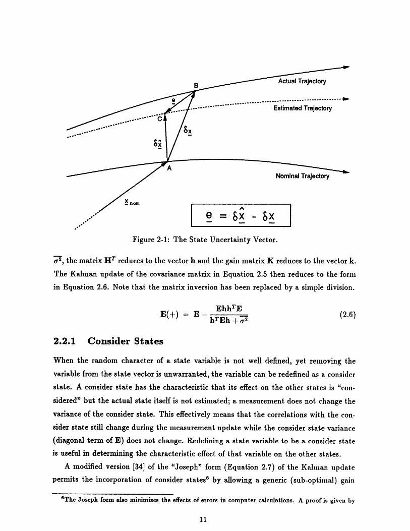
A graphical representation of this equation using only three states is given in Figure 2-1.

e = ,X- x = (xno + bX) - (xnom± + ) = bi - SX (2.1)

The vector being estimated is actually 6x. For an unbiased estimator (filter), the mean

error in the estimate is zero. Thus, e post-multiplied by its transpose is exactly its

covariance, E. This relationship is shown in Equations 2.2 and 2.3. Note that the E

matrix is symmetric.

= SiX-6x = 0 (2.2)

E - (e - )(e - )T = eeT (2.3)

The Kalman Filter uses the E matrix, the sensitivity matrix s of the measurement

(H) and the measurement error statistics matrix (R) to weight each measurement in

such a way as to optimally estimate the state. The matrix form of the sensitivities

and measurement statistics will be given in Sections 2.4 and 2.5, respectively. The

measurements in this study are taken to occur at discrete moments in time instead

of continuous measurements. Equations 2.4 and 2.5 are the standard discrete form of

the Kalman covariance update (see Gelb [14], pg. 110). The matrix K is the Kalman

gain matrix that adjusts the "weight" given the measurement. The matrix H is the

measurement sensitivity matrix described in Section 2.4. The "+" denotes the matrix

just after the measurement.

K = EHT[HEHT + R]-I (2.4)

E(+) = (I - KH)E (2.5)

The matrix I is the identity matrix commensurate in size with E. For a scalar

measurement (such as the angle between lines-of-sight to a star and a planet) of variance

4In a purely navigational analysis, 6x is taken to be zero. However, guidance is also to be examinedin Chapter 3 and requires six additional states in the state vector describing 6x, now non-zero.

sAlso called the measurement partial, but more correctly, the Jacobian.

Actual Trajectory

Nominal Trajectory

-nom Ae = e 8xeFigure 2-1: The State Uncertainty Vector.

r2 , the matrix HT reduces to the vector h and the gain matrix K reduces to the vector k.

The Kalman update of the covariance matrix in Equation 2.5 then reduces to the form

in Equation 2.6. Note that the matrix inversion has been replaced by a simple division.

EhhTEE(+) = E - hTE (2.6)hTEh + 02

2.2.1 Consider States

When the random character of a state variable is not well defined, yet removing the

variable from the state vector is unwarranted, the variable can be redefined as a consider

state. A consider state has the characteristic that its effect on the other states is "con-

sidered" but the actual state itself is not estimated; a measurement does not change the

variance of the consider state. This effectively means that the correlations with the con-

sider state still change during the measurement update while the consider state variance

(diagonal term of E) does not change. Redefining a state variable to be a consider state

is useful in determining the characteristic effect of that variable on the other states.

A modified version [34] of the "Joseph" form (Equation 2.7) of the Kalman update

permits the incorporation of consider states6 by allowing a generic (sub-optimal) gain

'The Joseph form also minimizes the effects of errors in computer calculations. A proof is given by

vector k'. The form is also computationally efficient with no matrix multiplies. The new

gain vector (for a 3 x 3 example) is given by Equation 2.8.

E(+) = (I - khT)E (I- khT)T + •~kkT (2.7)

k' [kik2

0

For this case, the updated covariance is

ell

e12

e13

e12 e13

e22 e23

e23 0

(2.9)

(2.8)

The form for the update equation is now

E(+) = E- (wwT _ wIwT)

hTw +C 2

0 (h )(k - k)w'= 0 = (hrEh+ •,2)(k- k')

W3

The inclusion of a consider

optimal gain. Another way of

By including the factor (1 + P)

measurements can be reduced.

state changes the gain from the optimal gain to a sub-

achieving a similar effect is through "underweighting."

in the calculation for the gain matrix, the sensitivity to

kunderweighting = (1 +)hEh + (2.11)(1 + +)hTEhT + +(2

Typical values for / are between 0.0 and 0.2. Underweighting is typically used when

the operating region has become somewhat non-linear. Reducing the sensitivity keeps

the filter from optimistically estimating the state far from the nominal. Non-linearity is

not expected in the interplanetary case so the factor P is not included in the simulator.

Battin [3], pg. 677.

where

w= Eh,

(2.10)

Underweighting is more often used for sub-optimal "tuning" of onboard filters rather

than in pre-mission covariance analysis.

2.3 State Propagation

Once E has been updated at a specific time by one or more discrete measurements, it

must be propagated in time to the next measurement time. This is done by linearizing

the equations of motion for the position and velocity errors about the nominal trajectory,

and assuming a linear form for the other bias states. This section gives the propagation

equations first for position and velocity errors, then for the bias states, and finally for

the covariance matrix E itself.

2.3.1 Position and Velocity States

The two-body non-linear equations of motion (EOM) for position and velocity are

r = v v = -9r (2.12)

where ir, is the unit position vector. A simple Kepler routine is used to evaluate the EOM

at any time given the initial conditions. Linearizing about the nominal state, x,,,,, the

first order linear differential equation for propagating state errors is

6x = F(t)bx (2.13)

where

F = G 0 (2.14)

and G is the gravity gradient matrix given by

G = 3u r (2.15)

Equations 2.13, 2.14, and 2.14 will be important when deriving the propagation equa-

tion for E in Sections 2.3.3 and 2.3.4.

Large Time Step Formulation

The propagation of the state via direct integration becomes cumbersome if at each point

along the trajectory, the effect of a measurement on some performance criteria at the

end of the trajectory is checked. The number of calculations is then nearly squared7 .

An alternative method is via the state transition matrix, T(tl, to). The state transition

method propagates the state error vector from time to to time tl in a single step. The

matrix is found by linearizing the state at time tl about the reference state at to.

x (t,x(to)) = X(t1,x,,ef(to)) + (X(to)- xre(to)) + 02 (6xo) (2.16)

xVo)=X(t 0o)IXretE) 6x

(tx1 t(2.17)

6X ~ x 1 = (tl,to)6Xo (2.18)

The cartesian form for 41 is well known. Shepperd's [35] derivation is implemented

in the simulator to propagate the state just after a measurement to the Mars encounter

date. Two other possibilities exist for calculating the 4I matrix.

Element Formulation

For very large time steps, generally on the order of multiple orbits, an element formulation

is often used. In this case, a different development for the measurement partials from the

previous section is necessary. The advantage of using a two-body element formulation is

that f is generally very simple; differing from the identity matrix by only one component.

Using the equinoctal element set, let

'The total number of integration steps would become: N = n(n + 1)/2 where n is the previousnumber.

100000

010000

0 01000 0 pelement 0 = a = -1.5 At - (2.19)

0 0 0 1 00 a5

000010

a00001

where a is the semi-major axis. The above matrix reserves the first element for the

semi-major axis and the sixth for the mean anomaly difference. After the simple prop-

agation for small deviations in the elements, the results can then be transformed into

cartesian coordinates. Shaver [32] gives the necessary transformation (Jacobian) matrix

if equinoctal elements are used.

Small Time Step Formulation

Of course, 4 can be applied to small time steps as well as large time steps. The transition

matrix is related to the dynamics matrix F by differentiating Equation 2.18, and using

Equation 2.13 to get

I = F l(to, to) = I (2.20)

In theory, this may be integrated to get f(tx, to). However, for short time spans, F can

be taken to be approximately constant so that, as shown by Gelb (see [14], pg. 60)

4(tl,to) = eFat (2.21)

Further, the short time step assumption allows Equation 2.21 to be linearized" as

O(tl,to) - I + FAt (2.22)

2.3.2 Bias States

The other filter states - biases - must also be propagated in time to the next measurement

time. A bias can be thought of as either constant or varying in time. If time varying,

'However, the time step allowing F to be considered constant may be different from the size of thetime step allowing this next linearization step.

it is generally both stochastic and a continuous function 9. In that case, the state bias

values, being continuous functions, are considered well correlated with their immediately

prior values. However, they are also considered largely uncorrelated with values distant

in time (having large r, where r = tl - to); having noisy characteristics. An exponential

autocorrelation function (0,, = _2e-M1l)1o with an appropriate choice of time constant P/

is a very useful mathematical model of this characteristic. The noise that forces the bias

to change is taken to be white noise. For linear propagation, the propagation equation

for each scalar bias state is

= Fx + Gn (2.23)

where F and G are constant, and n is the instantaneous value of the noise. This form is

precisely that of a first-order Gauss-Markov Process or ECRV (exponentially correlated

random variable). To find F and G, the simple shaping filter problem must be solved. The

desired ECRV power spectral density o,, is the Fourier transform of the autocorrelation

function, or

2s) = =T2,8q (2.24)

With 4o as the spectral amplitude of the white noise, the linear propagation equation

for a ECRV is

S= -PX + 0o n (2.25)

The second term of Equation 2.25 will be dealt with in Section 2.3.4 as process noise.

The first term has the same form as Equation 2.14 and yields the state transition matrix

for the bias states

e,,,v(t, to) = exp(-f3(tl - to)) (2.26)

The 15 x 15 F and 4 matrices for the entire state vector are

9 For a fine enough time scale. The function may look discontinuous on practical scales.10For a stationary process where T2 is the mean squared value of the error in the bias.

Fr,v 0

F = o [ (2.27)

0 --rd

4(tj, to) =

0]r,v 0e- o* ( x-to) 0

(2.28)

0 e-# ,(t -t-)

2.3.3 Propagation of the Covariance Matrix

The propagation of the error covariance matrix can be accomplished with the use of

the state transition matrix or through direct integration. The propagation of the actual

state and the estimated state differ by the addition of an extra term (process noise) to

the actual state propagation equation. The extra term will be discussed in the following

section (2.3.4) as it requires a detailed explanation. The propagation of the state error

vector is then given by

el = ai - x1 = O(t1,to)6:o - (tl,to)6xo = (t1,to)6, (2.29)

By post-multiplying Equation 2.29 by its transpose and taking the expectation, the

propagation equation for the error covariance becomes:

E(t 1) = "(t, to)E(to)•4"(tx,to) (2.30)

Gelb (see [14], pg. 77) shows that the equivalent differential equation is:

E(t) = F(t)E(t) + E(t)FT(t) (2.31)

Equation 2.31 is one form of the matrix Riccati equation. Both of these equations requirethe initial condition E(to) = Eo.

2.3.4 Process Noise

The above discussion has been limited to modeling only the dynamic effects of the equa-

tions of motion. In fact, however, the s/c is influenced by other unmodeled forces such as

gravitation from the planets, solar wind, s/c ventings and outgassings, jet firings for at-

titude control or momentum dumps, and aspherical geopotential effects near both Earth

and Mars. Run-time truncation (finite word length computer) error is also a source of

error11. Generally these effects are very small and considered perturbative forces, having

only a small effect on the two-body trajectory. In a detailed simulation, models describing

each force can be implemented. However, the models are not included in this simulation

for two reasons.

First, little additional insight is gained when the navigation problem includes these

extra force models. Considering that the navigation problem is primarily concerned with

the state error vector characteristics, and that all variables and parameters are evaluated

on the nominal path for this linearized study, the effects of the extra forces on the

state error vector is equivalent to merely using a slightly different trajectory. Secondly,

the extra force models generally require a significant amount of processing. For the

navigation problem, the important issue is the portion of the perturbing forces which

cannot be modeled, or will not be modeled as a matter of practicality. By lumping the

uncertainties of the various models into a single term called "process noise" (PN) 12, and

adding the term to the propagation equation in an appropriate manner, the navigation

problem is assured to be more realistic.

Position and Velocity

The process noise vector n must be included in the propagation equation for the actual

position and velocity state errors. The estimated state error vector is not subject to

process noise.

"x = F(t)6x + n (2.32)

~t = F(t)6^ (2.33)

e = 6i5- bx (2.34)

11Mease [27] claims that finite word length is the dominant error source for a detailed modeling ofgeostationary satellites.

12Rather than completely neglecting the perturbing forces.

The vector n is usually assumed to be white noise entering only into the three velocity

components of the equation of motion. The propagation of the E matrix is found by ap-

plying the matrix superposition integral to Equation 2.34, multiplying by its transpose,

taking the expectation, reordering the integration, taking the state error to be uncorre-

lated with the noise, and noting the form for the autocorrelation function for white noise.

The resulting propagation equation is

E1 l= (t1 ,to) Eo~T(t1,to) + t (tl,r) Q T(tl,r)dr (2.35)

0o 0with, Q -

0o I

where $Po is the spectral density of the white noise (the total value of the lumped un-

modeled uncertainties) in units of length squared per time cubed. Gelb (see [141, pg. 77)

derives both Equation 2.35 and the matrix differential equation for E:

E = FE + EFT + Q (2.36)

Appendix A provides an explicit derivation of this equation. Direct integration of

Equation 2.13 is the primary method used for covariance propagation in the simulation.

A fourth-order Runge-Kutta integration scheme is used. Since only the deviations from

the nominal state are considered and those deviations are small, an integration step size

of approximately 1/100th of the orbital period is used to obtain results with negligible

second-order error. The typical measurement frequency (and thus largest integration

step size) will be one day which is on the order of 1/400th of the orbital period.

Before both Equation 2.35 and 2.36 can be used by the simulator, the matrices Qand N must be assigned. The value for Q used is 1.05 x 10-1nm2/s3 for Mars approach

navigation [33]. The value for interplanetary space is expected to be lower as the various

perturbations due to the near-Martian environment are practically nil. The matrix N

on the other hand is much more difficult to assign. For this reason, Equation 2.36 is the

preferred method for propagation.

An analytical evaluation of the noise covariance matrix N is difficult for general

Q(t). However if Q(t) can be considered constant over the time span At = tL - to,

an expression is possible (see McClain [25]). If this span is equal to the time step of

the integrator for Equation 2.36, then the integration and state transition methods are

equivalent. McClain's study uses an element formulation to simplify the quadrature

in N (see Equation 2.35). In this formulation, Q is not defined as above, but as a

small percentage of the combined solar radiation pressure and Jupiter perturbative forces

converted via Gauss' Variation of Parameters into an element representation.

Alternatively, it is possible to find an approximation of N(At) by expanding it in a

Taylor series and truncating the series after the fourth term. The derivation is shown in

Appendix A with the result being

I At34ol L At2' I ]N= [ 3

2 1(2.37)[ At2 t oI AttoI + At3(, oG

In Chapter 4 it is shown that for an Earth-Mars Hohmann transfer, At can be between

15 and 20 days at any point on the transfer and achieve final errors within 99 percent

of those values resulting from direct integration. This means that, in the absence of

frequent (e. g. daily) measurements, the state transition propagation formulation can be

used instead of the direct integration formulation when it is desired to see how the current

state knowledge propagates out to Mars (see Section 2.3.3). Equation 2.37 is used instead

of the analytic N of Equation 2.35 since its value of io is consistent with that of the

integration method.

Measurement Bias States

The second term in Equation 2.25 gives the form for the process noise of an ECRV. The

constant multiplying the vector n can be carried outside the integrals of Equation 2.35 so

that the effect on N is to be multiplied by the square of the constant. Doing so cancels

out the spectral density of the white noise, o, in Equation 2.38. Thus, for an ECRV, the

process noise term is independent of the "size" of the white noise driving the variation

in the parameter. The values of Q and N (now scalars) are given as

Qecro -~ 2 2,23au2 2-2#, (2.38)

N = o (2.39)Necrv= QC.c,u e 'dr = ( e'^)(2.39)

Equation 2.39 is possible since F for an ECRV is simply -P , leading to a simple solution

for 9 13. Note that a value of infinity for 8 indicates that the process noise between the

states at to and t is uncorrelated, while a value of zero indicates the states are fully

correlated (colored); indicating a pure bias.

Summary:

Process noise is intended primarily to account for unmodeled and unmodelable dynam-

ics. A truly optimal filter estimates all of the factors influencing the system - in effect,

estimating the entire universe. Process noise is also useful as a guard against filter

divergence 4 .

2.3.5 Performance Parameters

It is often of interest to examine the errors at the terminal time' 5 when evaluating the

performance of the navigation system. For example, suppose the present uncertainty,

propagated to the terminal point without any more measurements, indicates that the

s/c will be outside a pre-defined aerocapture window. This suggests that the current

navigation accuracy has not yet achieved the required performance and that further

navigation is necessary. Propagation to the terminal point shows the effects of current

errors on the terminal errors. This ability is often useful because it permits important

mission parameters such as periapse altitude'" and inclination at the target planet to

be seen as functions of the present navigation performance. The errors in these two

parameters are the figures-of-merit (FOM) for the present problem; lower values indicate

better performance.

Aerocapture is a more restrictive type of capture than a propulsive capture. Thus,

high performance navigation is required to meet the capture requirements and thereby

gain the fuel savings of aerocapture over a thrusting capture. Shepperd, Fuhry, and

Brand [33] define the requirements for aerocapture and show that success is dependent

largely on the vacuum periapse altitude error of the approach trajectory which corre-

sponds to the flight path angle and altitude errors at entry interface (EI). This section

1 SFor a stationary process, to can be set to zero.'4 See Section 2.2.1.16A terminal condtion other than time is also useful."leeriapse altitude equals the periapse radius minus the planetary radius.

develops the conic partials of the periapse altitude and orbit inclination wrt position

and velocity on the hyperbolic Mars approach trajectory. Then, under the assumption

of small deviations, periapse altitude uncertainties can be related to current state un-

certainties through Equation 2.40. Inclination uncertainty can be found in a similar

manner.

6• = Oh, 1 E (2.40)

Derivation of Periapse Altitude Sensitivity

The vector partial of the periapse altitude, h,, wrt the Mars-relative position and velocity

is desired. Using the well-known formulas for the orbital semi-major axis, a, and the

eccentricity e, hp, can be expressed as a function of the state vectors r and v.

2 VTV 1a-1 2 - - [v x (r x v) -= u,] (2.41)

h, = a(1- e) - rM (2.42)

where rM is the mean radius of Mars. The desired sensitivity vector is simply

Oh. a o8a= [(1- e) - a] Or av (2.43)

ax ae aeOr Wv

where the semi-major axis partials are

a = 2a2 'T _a = 2a2'V (2.44)Or r3 Ov it

It is convenient to break the triple cross product of Equation 2.41 into the sum of two

vectors and differentiate to get the following eccentricity partials:

Oe V ) I - vvT + U rf] (2.45)

Or LrL r

Oe = [2rvT - vrT _ (ryT) I (2.46)(v A

Derivation of Inclination Sensitivity

If h designates the Mars-relative momentum vector and ^poe is the unit vector in the

direction of the spin axis of Mars, then the orbital inclination is defined as

hos T h 00 < i < 180' (2.47)cos po Uoe__

Taking the partial wrt r results in Equation 2.48. Using the cross product matrix1l ,

designated with a superscript z, the equation can be rearranged and given by Equa-

tion 2.49.

. . Oi- sin i OOr

[ o.]Tl'

= 1 hh-UpoIe [h h3V

OhOr (2.48)

(2.49)= hn-vx i (\AIpole)-_polh sin i i

cosi

The partial wrt velocity can be found in a similar manner. By

the inclination partial wrt the state may be summarized by

Oiax

with,

1h sin i

defining a new vector w,

vxr(2.50)

(2.51)w = cos ifh - Uipole

An obvious problem can be seen

higher order solution is needed.

when the nominal inclination is zero. In this case, a

2.4 Observation Models

This section describes the measurement types considered in this study and derives the

measurement sensitivity vector h for each type. Three types are described: optical data,

from a star tracker, 1-way Doppler measurements of the s/c relative velocity (range-

17For example, h = -v x r = -vwr = [vi]T r; here vy is a 3 x 3 matrix.

rate), and 1-way ranging measurements. Of these, only optical data is considered truly

autonomous since it does not rely on any sort of cooperative ground-support.

2.4.1 Optical Measurements

The primary measurement type considered here is the central angle between a star at

infinite distance18 and the centroid of a planetary body. Knowing the position of the

near body, the direction of the star, and the angle between them places the s/c on the

surface of a cone whose axis is in the star's direction. A second measurement using a

different star and approximate knowledge of the s/c's present position places the s/c on

the line-of-sight vector between the s/c and the near body. A second near body must

be used to locate the s/c along the line-of-sight. For this problem, Earth and Mars

are used as the near bodies. As will be shown, these two near bodies provide adequate

navigational information for the Earth-to-Mars transfer mission. Venus, however, could

provide a significant measurement source for an inbound trajectory, depending on its

location during that mission. For several reasons, the Sun has also not been chosen. First,

the Sun would require an additional instrument onboard the s/c; a sun tracker, quite

different from a star tracker by design, not theory' 9. Second, while better centroiding

of the solar disk is possible, the overall system accuracy (covariance reduction), which is

more sensitive to the long optical lever arm from the s/c to the Sun, is worse.

Two additional points must be made concerning the Sun and optical measurements.

First, suppose the s/c is near Mars and observing the Earth. It is possible that the

position of the Earth is such that the Sun occults or washes out the Earth. In addition,

the combined motion of the s/c and the Earth may prolong the occultation for days,

possibly weeks. The same is true for a near-Earth s/c observing Mars. Fortunately,

the effect is naturally avoided for manned mission scenarios. This mission generally

requires a relatively direct transfer of short duration. The possible geometries under

these restrictions do not permit the Sun to occult either planet.

The second point concerns the availability of stars near the sun. Lundberg [23] states

that, "even when a well designed sun shade is used, star sensors are typically inoperable

to within 30 to 60 degree of the sun." Obviously this effect places operational constraints

8sFor a complete mission design, errors in parallax and stellar direction should be taken into consid-eration, especially for interplanetary missions.

'9Sun sensors have been developed with 10 s'c accuracy - see Lundberg [23]

on the mission, yet in practice has almost no effect on the s/c's ability to navigate.

There are a number of possible designs for the angle measuring system, each with

advantages and disadvantages. One possibility is to use two independent star trackers,

each obtaining one of the visual bodies. If the measurements are not simultaneous, then

an inertial measurement unit (IMU) is required to track the motion of the s/c between

measurements. Another setup is to use only a single tracker, either narrow or wide field-

of-view (FOV), to target one body and then rotate the tracker boresight to the next

target. The single star tracker could be moved mechanically in a gimbaled platform

configuration or via slewing the entire s/c in a strap-down configuration. The platform

configuration is generally more accurate and does not require the fuel expenditure of

the strap-down type. Both configurations require the involvement of an IMU since the

measurements are not simultaneous.

Alternatively, the star and planet could be both placed within the FOV of the tracker.

The greatest advantage of this setup would be to eliminate the errors introduced by

IMU involvement. However, the disadvantages are significant as well. By placing the

two bodies in the same FOV, the size of the star catalog must be large to include the

lower magnitude stars. When using faint stars, there is always a risk of confusion and

the possibility of not being able to pick up the star at all. The problems of centroiding

remains for all device setups. For this analysis, the differences between the configurations

lie only in the choice of states to be estimated and in the accuracy chosen for the star

tracker (see Section 2.5).

Some trade-offs must be considered when choosing the mechanical configuration.

Lundberg [23] makes several points:

Large field of view instruments will have a relatively low resolution com-

pared to small field of view instruments, but the small field of view instru-

ments will require a greater pointing accuracy to view the intended target.

Also, in the case of strapdown instruments, a small field-of-view instrument

will not have a target in sight for as long of time as a large field-of-view

instrument will.

Other possible types of optical measurements use two near bodies, horizon detection,star-landmark angles, and star elevation angles. These have not been implemented for theinterplanetary navigation simulation since the latter two are only effective (and possible)near the planet, and the former is ineffective compared to the star-planet measurement

for geometrical reasons 20.

Sensitivity with Respect to Position and Velocity

When a measurement is taken, the partial derivative of the measurement wrt the state,

evaluated at the nominal state, is used by the filter to improve the error covariance as

described in Section 2.2. With .ta,, and ii,, representing the unit vectors from the s/c

to the star and planet to the s/c, and A representing the angle between the two vectors,

the measurement partial can be derived, beginning with

rre•Tcos A = st ,,aer (2.52)

andOrrel Orrel Orrel T -T

TIuOrrOrscre l rel (2.53)

Taking the derivative of Equation 2.52 wrt the inertial position vector, r,/c, yields Equa-

tion 2.54.

BA

fa cos A - rdr sin A (2.54)Ure Icos A-rIs Or,/C Ustar (2.54)

Rearranging gives

OA 1 [cosA B re+ At, (2.55)

ar/C rel sin A

The measurement partial h is to be evaluated on the nominal path at the measurement

time. In this analysis, the angle A is assumed to be 900 for each of two star measurements

in orthogonal directions. Figure 2-2 shows the measurement geometry. There are two

reasons for making this simplification. First, by fixing the angle, no extensive star catalog

need be implemented or searched by the simulator. Though this might seem to suggest

that obtaining both star and planet in the FOV has been eliminated, this is not the case.

In fact, the specific angle is largely unimportant until A becomes very small2 .

So far, the timing of the measurements has been assumed to be exactly known. Of

course, errors in the onboard clock actually exist. If the timing errors are expected to be

20For the missions studied, a significant portion of the journey yields little geometry variation andnear 180* orientations for inner planets and large lever arms for outer planets.

21 As Battin(see [3], pg. 635) proves, the sensitivity of the measurement to errors in computation isgreatest when the error is small as is readily seen by the sine term in the denominator of Equation 2.55

LOS

Figure 2-2: Relative Geometry for the Optical Measurement: A single planet-star mea-surement places the s/c on the surface of a cone. A second cone (measurement using thesame planet but different star) places the s/c on the line-of-sight unit vector with theplanet. Further measurements with the same planet do not help. In the present analysis,each cone is flattened into a plane.

large, they should probably be estimated in the state since these errors can significantly

affect the accuracy of optical measurements during conditions where the observation

geometry is changing rapidly. Battin ([3], pg. 641) provides an example of how the

measurement partials would change with the inclusion of timing errors. Results of studies

that include timing errors are given in [2] and [39]. Timing biases (and drifts) are not

expected to be a problem for the interplanetary portion of the journey and are not

modeled in this analysis. For the same reason, biases in the position (ephemeris) of the

planet and direction of the star are not modeled.

Sensitivity With Respect to Angle and Centroid Biases

While the partial of the angle wrt velocity is zero, the partials wrt the angle and centroid

biases are not. Figure 2-3 shows the typical arrangement of the measurement wrt the

internal coordinates of the star tracker and pixel array. Though all four biases exist for

any one measurement 22, only two of the biases will be observable if the measured angle

SP is aligned with either X or Y axis. This arrangement"2 is necessary since actual stars

22The determination of the centroid determines the attitude of the angle wrt the pixel alignment.2 30r a different but constant arrangement.

X - axis

Y - axis

.. .. . .N X. . .. . . ... \. \....\.......

G b* Nr *

SP

*A* ota

Figure 2-3: Example Star Tracker Pixel Array: The origin is at O while the actual inertialtracker origin is aligned to Ob. The measurement biases are 01, 02 and the centroid biasesare cbl, cb2. Two assumptions made in this analysis are that - = 900 and SP = 00 or900.

are not used by the simulator. The partial of the in-plane angle wrt an out-of-plane

bias is zero. The partial of the angle wrt the same-plane angle bias is simply one (a

one-dimensional unit vector). The partial of the angle wrt the same-plane centroid bias

is easily derived. If the ratio of the centroid bias to the relative distance to the planet is

small, then the error in the angle due to the bias is approximately

Aact =Ameaa +tan- 1 bdAmes + bd(2.56)t = A100D 100D (2.56)

where b is the bias in units of percent, d is the planet diameter, and D is the distance to

the planet center as shown in Figure 2-4. The measurement partial is now a scalar and

is given by

OA,,t dOb 100D

h T = (2.57)

(NOT TO SCALE)

old

Figure 2-4: Geometry of the Same-Plane Centroid Bias: D is the distance to the planetcenter and d is the mean planet diameter.

2.4.2 Radiometric Measurements

Under certain circumstances, 1-way ranging and range-rate (Doppler) measurements

qualify to some extent as autonomous data types. Here, the radiometric measurement

signal is transmitted from a known position and velocity and received by the s/c. The

data is then 1-way; received by the spacecraft. Though the s/c will necessarily have

its own transmitter used for communication, the transmitter is not used for navigation

since autonomy is assumed. The measurement partial hT is readily derived for range

measurements, but for Doppler measurements it is more involved as may be seen below.

The measurement partial of range wrt position has already been given in Equa-

tion 2.53. The range drift is modeled as a consider state, and the partial wrt the velocity

is zero. Battin [3] presents a clear derivation of the measurement partial for Doppler

data beginning with Equation 2.58

rreg

rl Vrel cos 0 = rrel ' Vrel (2.58)

Taking the derivative wrt both position and velocity, the desired partial is found in

Equation 2.59. Rearranging gives a better form of the Doppler measurement partial:

AM

?k

T ( rel VreT T

hdoppler -=e [ V 1 (rl re (2.60)

2.4.3 Optimum Measurement Selection & Scheduling

At any one time, a number of possible observations can be made. Not only are various

optical and radiometric measurement types available, but so are various stars, planets,

and transmitter locations (i. e. not only the DSN locations but possibly a communications

orbiter at Mars). Of course, not all combinations are possible at any one time, nor

would nearly identical observations yield additional information. Selecting a certain

combination for each moment in time that yields the most beneficial information becomes

important when few measurements can be made or when a large accuracy disparity exists

between the measurements. Battin (see [3], pages 687-694) provides a foundation for

optimizing the measurement type selection and schedule.

Optimization of the measurement selection can be accomplished with regard to posi-

tion error, velocity error, upcoming course correction error, or any other condition. Since

the simulation uses no real stars (only fictitious stars placed in pre-set optimal directions;

see Section 2.4), there is no need to implement an optimum selection scheme.

The optimization of the entire measurement schedule differs from a complete set of

singularly optimum measurements. Rather, an optimum schedule is one which allows

the terminal performance parameters to be minimized. Optimization of the measure-

ment schedule requires a priori knowledge of the measurement errors and of the guidance

errors. Real-time optimization is thus impossible but can be approximated by an iter-

ative off-line simulation. Of the studies investigated, most attempt to "optimize" the

measurement schedule only by eliminating those measurements that would obviously

yield no new information. Only Denham [9] has attempted to explicitly optimize the

schedule. Amazingly, Denham also treats the problem of optimal velocity scheduling

(see Section 3.6) in conjunction with the optimal measurement problem. This simulator

does not implement an optimization scheme. Instead, many measurements (relative to

previous studies) are taken so that those near-optimal measurements will be included in

the schedule.

2.5 Navigation Instrument Errors

This section discusses in detail present-day optical navigation instruments and their

associated sources of error. Accuracies for radiometric data will also be quoted.

Optical Instrument Errors

There are many error sources which limit a star tracker's ability to provide accurate

angle information. One particular error source, measuring the direction to the planet

center-of-mass, or centroiding, is a major contributor to star tracker error. For an out-

bound journey, it is likely that the Earth will be nearly new (as opposed to full) wrt

the s/c at some point along the trajectory. This has a large impact on the detectability

and centroiding capability of the sensor. For this study, the instrument error will be

considered as either a constant detection (and centroiding capability) or as the root-

mean-square (rms) average capability. Duxbury [11] breaks centroiding errors down into

more specific components:

1. Limb darkening

2. Marked albedo variations near the lit limb

3. Atmospheric uncertainties: altitude, composition, etc.

4. Algorithm defining the lit limb

5. Uncertainties in the target planet figure and spin axis orientation wrt the instrumentcoordinate system

6. Differences between the planet optical center and center-of-mass

7. Electrical and optical geometric distortion of the image

8. Photometric distortion of the image due to image plane sensitivity nonuniformities

9. Instrument calibration errors

Stanton et al. [37] cites a figure of 1% of the target diameter as having been achieved

for regularly shaped images for the ASTROS II star tracker. This will be the value used

for the baseline case discussed in Chapter 4. Other tracker errors arise from several

sources [23]:

* Spacecraft motion and mechanical jitter in maintaining star tracker boresight align-ment with the target centroid (especially true for manned spacecraft)

* The accuracy to which the bore axis is known in relation to the tracker pixel array

* All other mechanical alignment accuracies resulting in transformation errors

* Errors in the star catalogs may be on the order of 1 sec

* Parallax uncertainties for nearby stars (the modeled stellar parallax is 2 x 0.76 sefor Alpha Centauri)

There are three recent studies by Armstrong [1], Lundberg [23], and Stanton [37] that

cover the development of optical star tracking devices up to 1987. Between the three,

they offer over 150 further citations covering the accuracies of optical star trackers since

the early 1970's. Below is a list of five star trackers and their characteristics. All track-

ers are based on charge-coupled device (CCD) technology, perhaps the most significant

navigational development since the late 1960's.

1. The ASTROS tracker developed by the Jet Propulsion Laboratory:

* A 2.2 x 3.5 degree FOV, 340 x 512 CCD array* Measured noise at 0.3 sie, uncalibrated accuracy of 4 sie (la)

* Power consumption of 38 Watts

* Observable visual magnitudes from -0.8 to 8.2

2. The Retroreflector Field Tracker (RFT) developed by Ball Aerospace:

* A 8 x 8 degree FOV, 256 x 256 Charge Injection Device array

* Measured noise at 0.23 is' (0.5 s update), uncalibrated accuracy of 4 s- (10)


* Observable visual magnitudes from 0 to 6

3. The MADAN tracker developed by TRW:

* A 7.4 x 7.4 degree FOV, 324 x 324 CCD array

* Uncalibrated accuracy of 2.6 is (lo) for a 5.26 mean star magnitude


* Optics are defocused to give a. 2.5 pixel diameter star image which allowssubpixel position interpolation to approximately 1/50 pixel

4. HEAO-2 Mission Star Trackers:

* Employs three trackers, each with a 2 x 2 degree FOV

* Capable of viewing stars from magnitude 2 to magnitude 9

* 1.5 s~i (lo) accuracy after calibration

5. The ASTROS II tracker developed by the Jet Propulsion Laboratory:

* Developed for the deep-space environment: emphasizes low power and mass

* 256 x 256 CCD array


* Uncalibrated accuracy at 8.25 sie (lo)

* Able to track a point source to 10 mrad diameter,

* -3 to 10 visual magnitude.

Armstrong states that star tracker "accuracy is typically 1/20 pixel or better, giving

each tracker the potential for meeting star tracker requirements of 1 to 2 se." These

high tracker accuracies2 4 are in actuality rarely achievable even after on-orbit calibration

if it is necessary to incorporate the IMU into the measurement process as discussed in

Section 2.4. In this case, the IMU drift and its associated uncertainty that occurs between

the two sightings of a single measurement can be a significant factor in overall optical

measurement accuracy. To counter the gross effects of the drift uncertainty, an IMU

alignment (essentially a star tracker sighting) is performed periodically. Additionally,an error is associated with the alignment as well. A drift rate of 0.020/hour (1l) [24J

results in a 5 ise error after just 4.2 minutes. It is seen that the trade off between a

system incorporating an IMU and a system where both star and planet are measured

simultaneously on the same array can be large. With one system, a greater number of

bright stars can be acquired and tracked, but the IMU degrades the overall navigational

accuracy. With the other system, overall accuracy is improved but few stars are available,and acquisition is difficult. Though less accurate, the IMU and bright star combination

is more conducive to autonomous navigation according to Shepperd, et al. [33].

Radiometric Errors

Radiometric measurements are largely dependent on the stability of the signal fre-quency and the on-board clock characteristics. Jordan [16] cites a number of other major

24Lowes [21] states a 10 s'c (lo-) sextant accuracy in 1968.

error sources for radiometric data such as station location, polar motion, variation in

Earth rotation rate, ionospheric effects, and tropospheric effects25. As discussed previ-

ously, the errors are grouped for this analysis into a Doppler velocity bias, a 1-way range

bias, and a range drift parameter, all modeled as ECRV's. The range bias is due to

clock offsets, whereas the Doppler bias and range drift are due to clock drift rates. The

values for la radiometric errors have declined in the past two decades. Cicolani [6] cites

2-way ranging accuracies of 5.0 m plus 7.67 x 10-' meters per meter noise with no bias.

More recent data [24] gives ranging accuracies of 20 m bias and 1.4 x 10- 8 meters per

meter noise. One-way ranging accuracies are expected to have greater biases on the order

of 10 km because the timing errors between the transmitting and receiving clocks are

not canceled out26. The range drift value is calculated from the clock drift error times

the speed of light. For a Efratom Rubidium oscillator, the stability over one second is

approximately 1.0 x 10-11 seconds per second and 1.0 x 10 -120r -13 days per day [24].

The lo noise value for the range drift is then 0.003 m/s.

Range-rate accuracies have also improved. Cicolani [6] cites range-rate accuracies of

0.1 m/s noise with no bias. More recent data [24] gives ranging accuracies of 0.01 m/s

bias and 0.01 m/s noise. For comparison, two-way ranging and Doppler noise values are

15 meters and 0.001 m/s respectively [41].

2sNote that none of these error sources are modeled in the present analysis.28A clock drift of 1.0 x 10- 11 seconds per second yields a light time error of approximately 10 km.

Chapter 3

Guidance Theory

While navigation provides the spacecraft with an estimate of state deviations from a

nominal trajectory, "guidance laws" provide the capability to return the spacecraft to

that nominal trajectory. Cicolani [7] and Tempelman [39] both discuss linear impulsive

guidance laws in detail. This chapter discusses several laws, or schemes, that implement

linear impulsive velocity (Av) corrections - or Trajectory Correction Maneuvers (TCM's)

- and their associated execution errors. Also, an attempt is made to reduce the total fuel

costs associated with the course corrections by scheduling the TCM dates along the

trajectory. These laws require the 6 x 6 (position and velocity) state transition ma.trix

between the initial time (time of TCM application), tl, and the time at which the desired

end conditions are to be met, t2. The state transition matrix will be partitioned a.s

(t, t) 4k4 (3.1)

In the absence of process noise, the 4 and integration propagation formulations are

identical. However, the use of 4 is computationally more efficient for the relatively long

time intervals typically found in guidance and, more importantly, the 4 matrix allows

the guidance laws to be expressed in a general linearized form. An additional notational

covenience is to redefine for this chapter E, e, and bx, etc. as the six dimensional (position

and velocity) portions of their original 15 dimensional definitions.

Guidance theory is complex and intertwined with navigation. Ideally, guidance targets

the desired end condition and attempts to minimize the total Av and minimize the end

condition errors caused by the correction execution errors. These performance criteria

will be detailed further in Chapters 4 and 5.

3.1 Impulsive Assumption

This thesis follows the lead of most other interplanetary studies and approximates the

applied rocket thrust as an impulsive velocity correction instead of using a continuous

thrusting scheme such as cross-product steering to correct for state errors. If the burn

duration is short compared to the mission length, the impulsive TCM approximation is

perfectly adequate. The effects of the burn errors are of primary concern, with the total

burn cost being a secondary concern. Though the difference between 10 and 100 meters

per second total cost is significant, it is found that the burns are relatively small' com-

pared to pre-planned trajectory maneuvers such as injection, plane change, and capture

burns. Since aerocapture does not require a capture burn, the total mid-course correction

fuel cost is the more important factor. Also, a 10 m/s burn may last at most 1000 seconds

(s/c engines are expected to be proportionate to s/c mass). When compared with the

duration of the mission (approximately 10 million seconds for a sprint trajectory) and the

propagation method's step size, the impulsive burn assumption seems quite reasonable.

3.2 Fixed Time-of-Arrival Guidance

The most simple linear impulsive guidance law is Fixed Time-of-Arrival (FTOA) Guid-

ance. Here the desired end condition is to null any terminal position errors at the nominal

time of arrival (6rf = 0). The terminal velocity deviations are unconstrained. The deriva-

tion given by Murtagh et al.2 is simple and easy to follow. The derivation begins with

the position error at the nominal time of arrival as a result of the present state errors.

The position error at the nominal time of arrival after a velocity correction is denoted

by the "+".

Sr1 = F,6r + 426v (3.2)

6rf = 4,1r+ +4 26v+ (3.3)

An impulsive velocity correction implies that

1Usually less than 10 m/s. If a 1 cm/s error can cause a 1000 km final error, a 1 cm/s burn cancorrect for a 1000 km final error.

2[28], appendix D.

Av = 6v+ - v and 6r+ = 6r (3.4)

Equation 3.3 is now solved for the velocity correction resulting in

Av = 41' (b6r -~ r - 4 26v) (3.5)

Inserting the desired condition, 5ry = 0, into Equation 3.5, the expression for the FTOA

guidance law and the 3 x 6 guidance matrix, B, is given by

Avio = [-@I'1 -I] 6x = B6x (3.6)

The velocity correction to be applied is computed on-board the s/c with the estimated

state error, or AA^ftol = B 6S. The statistical representation of ^ftoa then depends not

only on the covariance of e, but also on the "covariance" of bx, the actual state errors

(recall Equation 2.1, page 10; 6S = e + 6x ). Thus, the dispersion matrix X, the

actual state correlation matrix is introduced3 by Equation 3.7. The characteristics of the

X matrix will be discussed in Section 3.2.1, but for the moment it is assumed that X is

available.

X _ =SxxT (3.7)

The Atý vector is a stochastic quantity whose descriptive correlation matrix may be

defined as

DV = AVA2T = B (e + 6x)(e + 6 x)T BT (3.8)

Equation 3.8 can be reduced to known quantities in the case of an unbiased estimator4 .

Battin finds that by pre-multiplying biT by e and taking the expectation gives

e(e + 6x)T = E + exT = 0 (3.9)

or

ebxT = -E (3.10)

aFollowing Battin's notation [3], pg. 681.4[3], pg. 677: e6•iT = 0 if either e or bi is initially zero.

The correlation matrix of the estimated velocity correction may then be rewritten as

DV = B(X - E)BT (3.11)

An additional quantity, though not necessary for the analysis, is the uncertainty in the

estimated velocity correction, DD.

DD - (AV - B6x)(AV - B6x)T = BEBT (3.12)

As Battin points out, "a velocity correction having a large uncertainty should not be

commanded if it is possible to improve the estimate substantially by future observations'."

Indeed, Battin gives a guidance scheduling scheme based on an rms velocity correction

uncertainty percentage and will be discussed briefly in Section 3.6.

Effects of the Course Correction

Once the course correction is calculated, it needs to be implemented. The errors that

are inevitably introduced by the TCM, called execution errors, are discussed further in

Section .3.5. The present discussion assumes the execution errors are zero. If the errors

are zero, then the state uncertainty remains unchanged.

E+ = E- (3.13)

The velocity components of the dispersion matrix, however, are modified.

6x+ = Sx+MBi: = (I+ MB)6x + MBe (3.14)

0where, M =

The matrix M is a "compatibility" matrix which applies the three dimensional correction

vector to the appropriate velocity positions in the state vector. Multiplying by the

transpose and using Equation 3.10 gives the updated dispersion matrix after the TCM

execution,

1[3], pg. 684

X+ = (I + MB)(X - E)(I + MB)T + E (3.15)

3.2.1 The Dispersion Matrix

This section discusses the definition, initialization, and propagation of the dispersion

matrix, X. The dispersion matrix is defined as the mean squared value of the actual

state errors 6x (position and velocity). Figure 2-1 on page 11 shows how the dispersion

state is related to the uncertainty state. Note that since 6x does not have a true mean

value, X may not be called a covariance matrix, but rather a mean squared correlation

matrix. An initial value for X is obtained by considering the initial estimated state error

j6 (not the uncertainty e) to be zero.

bx = 6x*-e, X x6xbx T , X0 = Eo (3.16)

The dispersion matrix propagates in exactly the same way as the error covaria~nce

matrix (position and velocity portion). However, if IMU drifts/biases and accelerometer

biases were also being estimated as part of the full state vector, X would propagate

differently6 . Using the state transition matrix propagation formulation as an example, it

is possible to write

E2 = I(t 2, t) El IT(t 2 , tl) + NX2 = .I(t2,tl) X1 IT(t 2,tl)+ N

This similarity suggests that these two equations can be put into a single equation

by incorporating the dispersion states into the full state vector. If this is done, one must

consider the possible effects of correlations between e and 6x. The assumption that the

noise is uncorrelated with anything other than itself leads to

Z = e6xT Z2 = 4(t 2 ,tl) Z1 IT(t 2 , tl) - N (3.18)

and

0 = bdiX = e, +6x x 0 = E + Z +Z + X (3.19)

"Kriegsman [18] gives a good explanation of IMU parameter estimation inclusion in the navigationcovariance matrix.

If Eo is symmetric, then Zo can be seen to be both symmetric and opposite in sign

to Eo: Zo = -Eo. For the position and velocity components at times tl and t2,

TE2 Z2 i [ El Z, F 0 N -NZ2 X2 O Z1 XJ 0 [ -N N

(3.20)

An analogous statement would hold for the differential propagation formulation. Now the

question is whether or not this propagation notation is necessary, especially in light of the

excessive zero multiplications. Although the G&N problem in this simulator is coupled

through the E matrix directly affecting X (Eqn. 3.15), and X indirectly affecting E

through execution errors (see Section 3.5), Z affects neither E or X in propagation or

thrust. Thus, why should Z be carried in the simulation at all?

The answer lies in the assumption of impulsive burns. In reality, the actual dispersion

state is only affected through propagation and the TCM's7 . If the simulation were to

estimate IMU errors and/or thrust errors to produce the burn, a non-impulsive propaga-

tion through the TCM would be accomplished through a different 4 (or F) which would

contain elements multiplying the Z correlations in the calculation of X. If this situation

is true, the form for Equation 3.11 may no longer be valid since Z has changed. A more

appropriate form would then be

DV = B(X+ E + Z + ZT )BT (3.21)

In addition to having to update Z, the equations for the update of X would also be

different (see Eqns. 3.22 and 3.23) while the update for E would remain unchanged.

X + = (I+ MB)X(I+ MB)T + MBE(MB)T +

(I + MB)ZT(MB) T + (MB)Z(I + MB)T (3.22)

Z+ = Z(I+ MB)T + E(MB)T (3.23)

7X is not directly affected by measurement incorporation since the actual state remains on its courseregardless of instrument readings and moves from that course only when a force acts on the s/c.

In this analysis, IMU errors are not part of the state and the TCM's are taken

as impulsive, negating the necessity for the propagation form in Equation 3.20. The

advantage of including the dispersion states in the full state vector is, for this simulator,

purely notational and not computational.

3.2.2 Potential Guidance Accuracy

It is typically thought that in the absence of execution errors and propagation process

noise, an FTOA velocity correction would null the position dispersions at the terminal

point. Indeed, if the pre-maneuver state is known perfectly, this would be true. However,

the state is known only to within the navigation uncertainty; thus, there is an uncertainty

in the calculated (best estimate) of the commanded Av. The matrix DD, the covariance

of the estimated velocity correction, is that uncertainty. DD is useful in gauging the

current efficiency of the burn and can be thought of as the "accuracy" of the TCM.

However, if the goal is to intercept at a point, the TCM accuracy should be taken as the

terminal miss at the desired target point. The following derivation shows that at any one

time, the guidance is limited by the navigation. The concept of a maneuver nulling the

terminal position dispersions in the absence of execution errors and process noise must

be abandoned when placed in a navigation-covariance analysis setting.

Let X- and X+ be the dispersion matrix before and after a velocity correction with

no execution errors. Let Xf be the dispersion at the final time. The error covariance,

E, does not change during the maneuver. No process noise is used in the propagation

of X + . It is desired to find Xf as a function of the present E and determine if, for a

FTOA correction, the final position dispersion is zeroed. Equation 3.15 is expanded by

partitioning the matrices into four 3 x 3 partitions as was done for the state transition

matrix

X+ = X_ -(x - E)~T~ E T + E2-[~' 1 (X- - El) + E3 -1If(X- - E,)f T-T + E4

(3.24)

Xf = ,(t1 ,to)X+4(t7,to)T (3.25)

Xf, = OX( t + 4 2X3f + 4X T + + 2X+ (3.26)

Next, the propagation Equation 3.25 is expanded to get Equation 3.26. Then Equa-

tion 3.24 is inserted into Equation 3.26. Canceling terms results in

Xf, = 41E,1 + 4 2E3 T + E3 1E2 T + f 2E4

= [(t,tto) E 4(tf, to)](1:s,1:3,)- position components (3.27)

Therefore, the best possible final position dispersion is exactly the partition of the present

navigation uncertainty propagated to the final time. For example, if the present uncer-

tainty of rms 30 km results in a 180 km final uncertainty after propagation (again, without

process noise), then the lowest rms dispersion attainable at the target with the guidance

scheme is 180 km.

3.3 Variable Time-of-Arrival Guidance

In the previous section the s/c was guided to an end condition at a fixed time. If

instead the time at which the s/c is to intercept its desired location is not constrained,

considerable fuel can be saved. This scheme is call Variable Time-of-Arrival (VTOA)

Guidance. Allowing time to "slip" is a useful tool if time is not a critical end condition.

Doing so provides a free parameter which can be used to minimize the TCM cost. FTOA

guidance is a deterministic problem: there are three end conditions and three control

variables - the thrust (Av) components. VTOA guidance uses the extra degree of freedom

to guide for the next most desirable condition: minimum fuel cost8 .

Murtagh et al. ([28], Appendix D) extends his FTOA derivation to the VTOA case in

a clear manner. The derivation begins with Equation 3.5. Instead of having brf = 0 ,the

linear approximation is made that bSr = -vfbt for some small, yet to be determined,

value of 6t. Here, v1 is the relative velocity of the s/c wrt the target (planet) at the

nominal time of arrival.

The new end condition is inserted into Equation 3.5 to get

Avt,, = 12 ' (-vj6t r-1 6r - 26v) (3.28)

8Fuel cost is just the magnitude of the estimated Av.

which can be rewritten as

Avvtoa = AVftoa - 921 Vb6t (3.29)

Next, Equation 3.29 is pre-multiplied by its transpose to get the squared magnitude

of the burn cost.

AVtoa = AVto - 2wTAvftoa6t + wTw6t 2 (3.30)

wherew = ilvf (3.31)

The derivative of the squared burn cost wrt 6t is taken and set to zero. The resulting

equation is solved for 6t and re-inserted into Equation 3.29. Lastly, the VTOA course

correction is found by pre and post multiplying the FTOA burn by an idempotent matrix:

0 = -2wTAvifoa + 2wTw6t (3.32)

Avo = WvtoaAVtT (3.33)

where

Wietoa I WW T(3.34)

DVvtoa = AVvtoaAVo = WvtoaDVftoaWto (3.35)

with WvtoBfto being the VTOA guidance matrix. The concept of minimizing the

correction vector is show graphically in Figure 3-1.

Murtagh points out that, "the extra degree of freedom may be used to control an

additional terminal deviation if desired," rather than using it to minimize the burn cost,

and gives an example for the flight-path angle. Gossner [15] develops this concept further

into a generalized scheme which will be used in the next section to develop two other

guidance schemes.

The Compensation Vector

In the VTOA problem the dispersions at the nominal time of arrival will always be

FTOA

VTOA, ..- \

Figure 3-1: VTOA Guidance: The vector w represents the locus along which a coursecorrection vector must terminate in order that the final position error be nulled. Obvi-ously, the minimum correction is perpendicular to w. The time deviation 6t is in genericunits.

larger than the FTOA dispersions. Because the time of intercept has been moved, the

time at which the guidance law attempts to zero the dispersions has been moved. This

new time is not the nominal time of arrival. Figure 3-2 shows this relationship. A

modified dispersion matrix X' is needed to reflect that the dispersions at the actual

VTOA intercept point are not large in an absolute sense, just large wrt the nominal

trajectory. Define the modified dispersion matrix to be

X' - aar (3.36)

Since only 6t2 is really known, the time (t + bt) of the actual intercept point is

unknown. Therefore, the simulation can advance only to the point at the nominal time

of arrival. Since the transition matrix from t,,, to tf is dependent on the knowledge of

bt, FC is approximated by AB and the compensation vector is defined on the path OB

rather than OC. With these successive approximations, it is easy to see that the vector

a is well approximated by the vector c, the FTOA dispersion. Thus, when analyzing the

dispersion in the VTOA problem, the FTOA dispersions give the desired information;

how far the s/c deviates from the path that targets the end point. The matrix X' is the

FTOA dispersion matrix and is updated using the DVft,, matrix but with the VTOA

execution errors (see Section 3.5). Note that in the calculations for the mean squared

velocity correction DVvtoa , the unprimed X is still used.

(NOT TO SCALE)

Figure 3-2: VTOA Guidance: The vector XE is the actual VTOA dispersion at thenominal time of arrival. The point C is the new intercept point. The vector C•E is thedesired quantity - the modified dispersion at the intercept point. The vector AC- is thevelocity of the target times bt. The vector b is the "compensation vector" (b = F-C).

3.4 Periapse Altitude and Inclination Guidance

This section gives several schemes for nulling an inclination and/or periapse altitude

error (see Section 2.3.5) at the target planet. These schemes are grouped under the

term "periapse guidance." The objective of a periapse guidance scheme is to null the

required states with a velocity correction costing less than either the FTOA or VTOA

methods. The emphasis is given since it shall be shown that both FTOA and VTOA

methods effectively null the periapse altitude (and to some extent, inclination) error.

The schemes presented here have been developed for this thesis and are only a small

subset of any number of schemes that might come under the label "periapse guidance."

The two schemes utilized in this thesis are derived here and the system performance for

each will be presented in Chapter 5. Several other methods are given in Appendix B.

Before beginning the derivations of the two schemes, a few issues must be addressed.

Depending on the guidance scheme, the state transition matrix 4 may be the product of

an elliptical (IE, to the Mars sphere-of-influence (SOI)) and a hyperbolic (OH, from the

SOI to the nominal periapse) transition matrix due to the patched conic approximation

being made. Each scheme will state explicitly the time at the target condition; either

SOI or periapse.

I

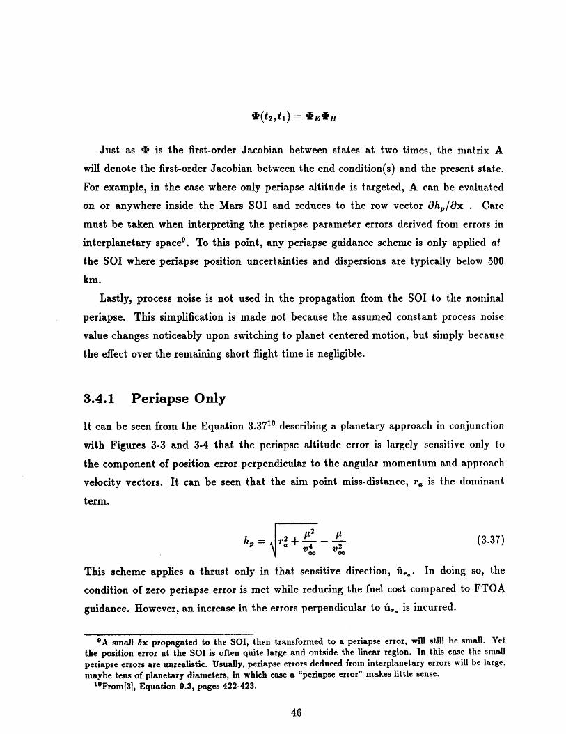
l(t 2,1t) = I7EIH

Just as 4 is the first-order Jacobian between states at two times, the matrix A

will denote the first-order Jacobian between the end condition(s) and the present state.

For example, in the case where only periapse altitude is targeted, A can be evaluated

on or anywhere inside the Mars SOI and reduces to the row vector hp/Ox . Care

must be taken when interpreting the periapse parameter errors derived from errors in

interplanetary spaces. To this point, any periapse guidance scheme is only applied at

the SOI where periapse position uncertainties and dispersions are typically below 500

km.

Lastly, process noise is not used in the propagation from the SOI to the nominal

periapse. This simplification is made not because the assumed constant process noise

value changes noticeably upon switching to planet centered motion, but simply because

the effect over the remaining short flight time is negligible.

3.4.1 Periapse Only

It can be seen from the Equation 3.371o describing a planetary approach in conjunction

with Figures 3-3 and 3-4 that the periapse altitude error is largely sensitive only to

the component of position error perpendicular to the angular momentum and approach

velocity vectors. It can be seen that the aim point miss-distance, r, is the dominant

term.

r2+ _ tL (3.37)

This scheme applies a thrust only in that sensitive direction, fi,,. In doing so, the

condition of zero periapse error is met while reducing the fuel cost compared to FTOA

guidance. However, an increase in the errors perpendicular to Ui,. is incurred.

9 A small 6x propagated to the SOI, then transformed to a periapse error, will still be small. Yetthe position error at the SOI is often quite large and outside the linear region. In this case the small

periapse errors are unrealistic. Usually, periapse errors deduced from interplanetary errors will be large,maybe tens of planetary diameters, in which case a "periapse error" makes little sense.

10From[3], Equation 9.3, pages 422-423.

8000

7000

5000

4000

3000

....... .... .. ........ .. .... ..... .. . ... .. .. ... ....... . .............. ... .. ... ....... .......... ..... ...... ....V................. 12 KM SEC

V 2 K /I SEC

--"3000 4000 5000 6000 7000 8000 9000 10000 11000

ra

Figure 3-3: Plot of Equation 3.37 for v~ of 2 -+ 12 km/s: Deviation from linearity beginsto show only below the surface of Mars with each curve finally reaching the origin (0, 0).The value for rM, the Mars mean radius, is 3393.4 km.

. 0-

S..w

4I C!

L-0L

0-a0

4),,

L - I VIII I I I300.0 250.0 200.0 150.0 100.0 50.0 0.0

Time to Encounter (days)Figure 3-4: Periapse Altitude Sensitivity to State Errors in a Mars LOS Coordinates:(coordinate definitions on page 71 and in List of Symbols) Z sensitivity is similar to theY sensitivity. The curves represent the peria.pse error produced by a mid-course 1000 kmor 0.1 mm/s uncertainty or dispersion for the Hohmann transfer described in Chapter 4.

rM

a 1000 m along X Line-of-Sightv 1000 m along y Line-of-Sighto 0.0001 m/s along X Line-of-Sighto 0.0001 m/s along Y Line-of-Sight

................. ..... ...... ......

I

Oa.C- w 1

Let T be the matrix that transforms from sun-centered inertial coordinates at the

SOI to a system such that the second component is aligned with the aim-point miss unit

vector ir,,

Ut,

Ub ] Ub = U, X iUh

where iih and i~, are the Mars centered inertial Mars-relative angular momentum and

velocity unit vectors respectively. A transformed position error vector is defined from the

propagated position error at the SOI as brr Tr,0o . To null h,, the second component

of 6 rT is set to zero so that the desired inertial position error at the SOI br',i is

1

6roi = T' 0

1

= T

O]0 T6r,o,

1

which yields the idempotent matrix form

br8,i =I - F 5r,0

(3.38)

(3.39)

Next, the propagation equation back to time

equation solved for Sv, using Wr, = tro.

to is applied to both sides and the

(3.40)165r' + ' 26V' = I- bilT] [ 16ro + , 26 0o]

Canceling terms gives

with

Av = 6v' - 6v, = B6xj

B = -12U'fibUb[1 21

(3.41)

(3.42)

Three points must be made about this method of obtaining Av. First, while the

method has nulled h, at the SOI, the method can be applied anywhere inside the SOI as

well requiring 4 to include a hyperbolic portion. Second, the method does not incorporate

any means to explicitly minimize the velocity correction. However, since the scheme is

effectively burning out only part of the error, the cost should be less than that of the

standard FTOA scheme. Lastly, the error is strictly FTOA.

3.4.2 Periapse and Inclination

This scheme is analogous to the FTOA - VTOA relationship presented earlier in this

chapter. Instead of guiding for the three end conditions b5r, 5r2, br 3 = 0 at periapse,

the desired conditions are 6hp, Si, 6t, = 0 , where 6t, is the nominal time of periapse

passage11. These new conditions can be met anywhere along the hyperbolic approach

trajectory since they are orbital parameters which, for conic propagation, do not change

after the TCM (in the absence of perturbing accelerations, i. e. process noise). However,

propagation to the SOI is still required. First, Sxsoj is transformed with the sensitivity

matrices A1 and A2 , defined as

Or Ov

A 1 = i A2 = I (3.43)

Or Ov

Solving the following equation for 6v yields the fixed time of arrival Equation 3.45.

[Shp0 = i = [A 2 A] IFx (3.44)

Avp~a, = [C - I] x (3.45)

C = -(A1k2 + A24 4 )-1 (A1,I + A2 I 3 ) (3.46)

Next, by letting &t, vary, the cost of the course correction can be minimized. A step

not shown in the previous sequence is expanded without setting St, to zero.

'v6 = (AlI 2 + A2 4)-1 0 t, - (A1 1 + A2 03) bri (3.47)

Now, if Equation 3.47 is divided into two parts, the VTOA method of Section 3.3 can be

11 8tO/Ox is undefined at periapse (see Appendix C).

followed.

Avvtoa = AVftoa + Wbtp (3.48)

w = (Alz2 + A2'4)-1 0 (3.49)

1

Avvtoa = wrw ftoa (3.50)

3.5 Burn Execution Errors

When the onboard system implements a TCM, burn execution errors result. The er-

rors may arise from fuel inconsistencies, inaccurate timing and pointing of the burn,

accelerometer errors, nozzle buffeting and a number of other sources. This section de-

scribes three ways to model and group these errors as well as show their effects on the

knowledge of the s/c state. This section is a very important part of this study, since

it provides the coupling between the navigation and guidance problems. The effects of

execution error on the accuracy of the final s/c state are shown in Chapter 5.

3.5.1 Known and Unknown Errors

There are two important types of execution errors: "known" and "unknown." Known

errors are the difference between the planned burn and the thrust actually sensed by

the IMU. Unknown errors are the difference between the sensed thrust and the actual

thrust. If the TCM is not sensed, there are only unknown errors. The distinction is im-

portant because, depending on the execution method, known and unknown errors affect

the state uncertainty and dispersion matrices differently. The execution method is one of

three general types: open-loop/modeled, open-loop/sensed, or closed-loop/sensed. Each

of these can be further broken down into two groups depending on whether or not param-

eters associated with the thrust and control (if any) are included in the estimated state.

For example, in the present simulator, no thrust scale factors, accelerometer scale factors

or biases, IMU misalignments or drifts, or clock drifts or biases are modeled as filter

states. But their effects are accounted for by process noise. The "open-loop/modeled"

option then becomes "open-loop/unsensed."

Basically, the sum of the known and unknown errors affects the dispersion matrix,

X, while only the unknown errors affect the uncertainty covariance matrix, E. In an

open-loop/sensed system the engine errors are measured but not acted upon (controlled

or countered). By assigning the engine errors and the measurement accuracy statisticallyindependent values (77 and C), the effects on E and X are independent and given below.

The next section will discuss how to obtain 71 and C.To show the effects, the errors 7 and C are first added to the velocity components

of Equation 3.14 and 6e+ = 6e. Assuming the errors are uncorrelated with either thedispersion or uncertainty vectors, Equations 3.13 and 3.15 become:

E+ = E+MNAMT (3.51)

X+ = (I + MB)(X - E)(I + MB)T + E + MNBMT (3.52)

where

NA = (T NB = + NA (3.53)

An open-loop/unsensed system means that the errors are completely unknown. A

closed-loop/sensed system assumes that the known errors are largely canceled out, leaving

mostly unknown errors. The errors inherent in these two methods will be different in

that the source of the errors will be different; engine and timing errors on the one hand,

and measurement errors on the other. For a well designed feedback system, the closed-

loop errors are presumably smaller. However, since the errors are integrated in time, this

conclusion is not necessarily correct. In both these cases NA r NB

3.5.2 Three Models

As mentioned previously, the execution method determines the source of the errors. This

section discusses the derivation of NA and NB. The matrix NA for a sensing system is

first considered. The statistics for NA should combine the effects of the uncertainties in

the IMU package. If biases and/or drifts associated with the IMU are estimated in the

state, a formulation for NA must be devised. This simulator, however, does not include

those states. Instead NA is assigned a certain value [6] [28], and a Gaussian uncorrelated

spherical distribution is assumed:

NA = C21 (3.54)

If the system is closed-loop, then Ns - NA . Otherwise, NB must be found as a

function of the statistics of the engine errors. By grouping the errors into magnitude and

direction errors, White et al. 12 extends Battin's derivationl 3 to include cut-off, or timing

errors. Cut-off errors become the dominant error source for small burns. Magnitude errors

can be thought of as proportional errors, and direction and cut-off errors as fixed errors.

By assuming each of the errors are Gaussian and uncorrelated with each other, White et

al. comes up with the following formula:

NB = + DV + 2 (I - DV) (355)C2 2 2

where c2 is the trace of DV and T2, 72, and E2 are the variances of the magnitude,

direction, and cut-off errors, usually given in percent, radians, and meters per second,

respectively.

The third system option is if the TCM is not sensed at all. In this case, NA = NB

where NB is calculated from Equation 3.55.

3.6 Course Correction Scheduling

The problem of deciding the time at which to implement a course correction is prob-

ably the most troublesome in designing an AG&N mission. Four conditions should be

considered when deciding to apply a course correction.

1. Is the magnitude above the minimum value executable by the engines? (Can the

correction be produced?)

2. Is the uncertainty in the TCM a significant percentage of the actual burn size?

How well is the maneuver aiming for the correct condition?

3. Is the amount of execution error a sizable portion of the correction itself and is the

time-to-go large enough to propagate these errors (with or without the presence of

12See [40], pg. 28, Appendix A.1aSee [2], pg. 682

subsequent TCM's) into significant final errors?

4. By applying the correction at the present time, will the sum total cost of all TCM's

be minimized?

Obviously, the first condition is the only necessary condition, while the latter are listed in

order of increasing desirability. This section develops two tools that give an approximate

answer for the second and fourth questions.

The first tool is presented by Battin 14. Here a ratio of the rms uncertainty in the

course correction to the rms size of the course correction is used as way of determining

whether or not to execute the course correction. If the ratio is below, say, 10%, then the

calculated burn should be executed. This condition may be written as

v/trace(DD) Strace(DD) 10% (3.56)Vtrace(DV)

The percentage could be allowed to change during the flight, presumably increasing as

the navigational accuracy improves, since it is the navigation accuracy that drives the

overall guidance accuracy. The drawbacks to this method are threefold. First, a course

correction must be calculated at each point on the trajectory and checked against the

criteria. Second, the date of the TCM is unknown prior to the beginning of the mission

since the mission navigation has not yet begun. Third, there is no guarantee that a.

correction will not be selected that is unreasonably large (though a check could be easily

implemented).

A second method, first given by Lawden [19] [20], selects the dates of the TCM's so

that the total correction cost is minimized (an "optimum schedule"). Cicolani [6] presents

a clear derivation of Lawden's scheme for FTOA guidance, and Murtagh [291 presents an

extension for VTOA and sub-optimal scheduling. Murtagh [30] gives fair treatment of

the assumptions made and describes the optimum scheduling problem as follows:

Given that N velocity corrections are to be executed between the time

of injection tl and the time of arrival at the target t2 , find the sequence of

these execution times such that the sum of the rms velocity corrections is a

minimum, subject to the constraint that the miss distance following the last

correction is equal to some specified value.

14[4], pg. 318.

The solution to the optimum scheduling problem depends upon both the

navigation system configuration and the guidance system configuration. Be-

cause of the dependence on the navigation system, the general problem is of

such complexity that no analytical solution has yet been proposed.

However, certain simplifying assumptions are made by Murtagh/Lawden in their

method that mitigates this problem. The method's assumptions are:

1. The correction schedule is independent of the observation schedule after the first

correction; effectively this means that DV = BXBT instead of Equation 3.11.

2. The cut-off error is the dominant execution error and is spherically distributed,

leading to DV -' trace(DV) I , or effectively, NB - F2 I. This is not true for

the first TCM. Modifying the first correction date and thus the post-burn miss can

keep the future TCM's small, so that this assumption remains valid.

3. The errors in making a correction are small compared to the actual correction. This

means that instead of Equation 3.52, Equation 3.15 is used. And, if assumption 1

is valid, Equation 3.52 is reduced further to

X+ = (I + MB)X(I + MB)T (3.57)

which means the desired target condition is actually attained, counter to the dis-

cussion in Section 3.2.2.

4. Perhaps the most restrictive assumption lies with the approximation

I 2(t1 , t) = (tf - t)I. This is essentially the same approximation used for VTOA

guidance. For very small velocity dispersions this may be valid over certain dura-

tions. For interplanetary trajectories, however, the assumption is clearly not valid.

The effect of the assumptions is to limit the scheme to a region where the trajectory is

nearly a straight line. Lawden's scheme is as follows:

1. Choose the date tx of the first correction, preferably close to injection to limit the

effects of large velocity dispersions. Time must be given to the navigation system to

provide accurate state (and thus correction) information. Obtain cl, the magnitude

of the rms velocity correction, and mi, the magnitude of the rms final miss after

the first correction.

2. Choose m., the desired magnitude of the rms final miss after the last correction.

3. Choose n, the number of course corrections to be implemented. The optimum

number is given by Lawden as

n = 1 +ln(Mi) (3.58)

4. Calculate the schedule with

i-I

tgo, = ( for i = 2,...,n. (3.59)

where tgo is the time to go before ma is to be attained.

In essence, the entire schedule is a function of ti. A quick computation for a typical

interplanetary trajectory shows that Lawden's method is unrealistic or impossible; either

the second TCM date is to be before the launch, or m, must be smaller than a reasonable

(autonomous) navigation system could provide.

A more intuitive scheduling logic is used in the Mars Observer [41] TCM scheduling.

Four scheduled burns occur on days 10, 30, 130, and 347 of the 356.9 day journey. The

first two TCM's concentrate on correcting for previous burn errors (injection and the

first TCM, respectively). The second two TCM's concentrate on correcting for orbit

determination errors built up throughout the interplanetary cruise.

TCM-2 is essentially a clean-up maneuver for TCM-1. At this point in

the mission, OD errors are not significant. TCM-3 corrects the execution

errors of TCM-2 and for the OD errors up to that point. The final trajectory

correction, was chosen to be near encounter so that execution errors would

not have time to propagate, and OD errors would dominate. The 10-day limit

before injection was set so that there would be sufficient time to improve the

orbit knowledge and update the MOI (Mars Orbit Injection)" s burn param-

eters before MOI. This limit also allows a period to perform an emergency

burn if necessary."'

I'The Mars Observer uses a propulsive capture rather than an aerocapture.16 See [41], pages 5-13

Lastly, Stern and Potter [38) give a different approach to the optimum scheduling

problem. Theirs is an interesting, deterministic approach not a.pplicable to this thesis

but is worth noting. Though few approximations are made, Stern's solution is graphical

and difficult to derive for a schedule containing more than two maneuvers.

Chapter 4

Typical System Performance

This chapter provides an example of interplanetary AG&N capabilities. A baseline mis-

sion and navigation system is defined and, by means of the computer simulation, the

performance is analyzed. The results of the simulation provide initial conditions for the

Mars approach simulation described in Reference [33]. A performance analysis of the

baseline scenario is made using defined figures-of-merit (FOM) for both the interpla~n-

etary simulation and the approach simulation. The analysis begins at the navigational

level followed by a guidance analysis. Chapter 5 presents some performance results forvariations about the baseline run.

4.1 Baseline Mission

In defining the baseline scenario, an attempt has been made to select those values that

both represent current technology and a realistically scheduled mission. The nominal

two-body trajectory of the s/c is defined first. Next, various navigation parameters suchas error statistics and an observation schedule are given. Lastly, the guidance errorstatistics and a correction schedule are presented.

4.1.1 The Nominal Trajectory

A Hohmann transfer is chosen as the baseline trajectory to provide the nominal positionand velocity vectors. Since the Hohmann transfer requires the smallest possible injectionvelocity (the factor driving fuel costs), it is assumed that an actual mission would be near-Hohmann. The paths of Earth and Mars are assumed circular and in the same plane as

the Hohmann path with the transfer going from Earth to Mars. The out-bound journey

is selected because it is probably the more difficult. Figure 4-1 shows the interplanetary

journey.

1.5

1

p 0.5

0

-0.5

-1

-1.5

2-

Figure 4-1: The Baseline Hohmann Trajectory: The spacecraft is labeled with the circle.Lines-of-sight connect the spacecraft and the planets at intervals of 12.9 days.

For this analysis, the transfer path cannot be a simple Hohmann or intercept path

produced by a Lambert routine since periapse altitude, h.p, and inclination, i , require-

ments at Mars are also to be met. The nominal values for hP and i are 20 kilometers

altitude1 and 45 degrees, respectively [33]. A patched conic method 2 is needed to match

the interplanetary position and velocity at the SOI with the Mars relative hyperbolic

state that results in the desired hp and i. Appendix D gives such a method. The initial

states for the spacecraft, Earth, and Mars in sun-centered inertial coordinates are given

in Table 4.1. The trajectory is inclined to the ecliptic by 0.06310.

Of course, Hohmann transfers do not occur in practice. In fact, missions generally

include broken-plane maneuvers and/or retargeting to further reduce fuel costs and meet

impact probability requirements. These considerations would change the nominal pa.th

in much the same way as would choosing an entirely different Lambert trajectory. By

1Above the Mars equitorial radius of 3393.4 km.2 Motion within the Earth's SOI is considered to be sun-centered - not influenced by the Earth.

58

.... ....

ii

.'' ... .. .

Spacecraft:

Earth:

Mars:

Position (km) Velocity (km/s)x 8.77750238e+4 3.27679774e+1y -1.49344822e+8 -8.03470642e-3z -3.47638576e+3 -3.61019597e-2x O.Oe+O 2.97846928e+ 1y -1.49597927e+8 O.Oe+Oz - 0O.Oe+O O.Oe+0Ox 1.59325053e+8 1.72559756e+1y -1.63011178e+8 1.66865771e+1z 0.0e+O O.Oe+O

p,,, = 1.32712499e + 11 km-/s 2

Table 4.1: Initial Conditions For The Three Bodies In Motion: Inertial Coordinates. Thegravitational constant for the Sun is also given.

selecting alternate single-impulse trajectories, more complex trajectories are represented

in the sensitivity analysis portion of this study (Chapter 5). Thus, the choice of a simple

Hohmann transfer as the baseline mission should not be considered overly simplistic.

4.1.2 Navigational Design

Covered here are those parameter values discussed in Chapter 2 that are necessary to

completely specify the navigation system. Staying within the scope of this thesis, "navi-

gation" (measurements) occur only on the interplanetary portion of the journey; namely

from the post-injection point to the Mars SOI. An analysis of the remainder of the

journey, from the SOI on down to entry interface and periapse, will be covered by the

simulation described in [33] and presented in Section 4.3.2.

Measurement Schedule

In the interest of maintaining autonomy, the baseline navigation system takes only optical

measurements. Sightings of both Earth and Mars are taken once each day, beginning at

the start of the journey up until the Mars SOI. Other studies [6], [28] take measurements

much more infrequently in deep space with the frequency increased nearer the planet.

By choosing a schedule that is more uniform, the sensitivity to measurements during

certain times of the journey are more readily obtained. Specifically, insights into the

sensitivity of the navigation to geometries created by planetary positions and planetary

motion (dynamics) can be gained.

Two measurements are assumed to be taken simultaneously for each planet (total-

ing four measurements). Each measurement pair measures the central angle between

the planet and two stars with mutually orthogonal lines-of-sight as previously shown in

Figure 2-2 on page 27.

Deimos is expected to become visible (visual magnitude of approximately 5) at about

26 days prior to Mars encounter3 for a Hohmann trajectory4 . Thus, at a more conser-

vative 20 days prior to encounter, Deimos optical measurements are subtituted for Mars

measurements. Twenty days is chosen instead of 26 to reflect the "slower" transfers

of Chapter 5 without modifying the baseline setup. The substitution is an attempt to

include the increasingly beneficial geometry variations Deimos provides as the s/c ap-

proaches Mars. In addition, because Deimos is a much smaller body, the centroiding

error effects are considerably smaller (though the centroid error itself is larger as a per-

centage of body diameter). Deimos has an approximately 30 hour orbit about Mars at

a mean distance of 23,459 kin. Measurements are taken at 15 hour intervals to obtain

Deimos at its maximum separation. Figure 4-2 shows the measurement configuration

for two Deimos sightings. At that point, Earth measurements are also taken at 15 hour

intervals for programming convenience. Mars measurements are not continued, as the

Deimos measurements provide better information.

LOS to Deimos @ 0 Hours D

.---.----- Mars LOS

SIC LOS to Deimos @ 15 Hours D

Figure 4-2: Geometry of the Deimos sightings: Mars-Deimos LOS is perpendicular tothe s/c-Mars LOS.

8"Encounter" is use here loosely as meaning the point at which the s/c crosses the Mars SOI.4 See Shepperd [36].

A Priori Covariance

Obviously, if only optical measurements are being taken, no radiometric parameters are

to be estimated in the state. The remaining states (see Section 2.1) have a priori statistics

as shown in Table 4.2. Each state is assumed to be completely uncorrelated with all other

states resulting in a diagonal matrix. There are several points that must be made about

the values of Table 4.2:

* The magnitudes of the a priori position and velocity errors (uncertainties and dis-

persions) depend largely on where the injection burn takes place. If the injection

burn starts in low Earth orbit (LEO), it may be possible to use the Global Position-

ing System (GPS) to reduce the post-burn state errors dramatically. The position

values given here are representative of an injection burn of 2.98 km/s performed

without benefit of GPS updates. In any case, it will be shown in the next chapter

that overall navigation performance is relatively insensitive to initial conditions (as

might be expected). For comparison, Murtagh [30] (1969) cites injection errors of 4

miles (6.4 km) and 16 fps (4.9 m/s). In addition, the lo s values used by Yen in [41]

for the Mars Observer mission are: 1.74, 1.86, and 2.25 kilometers and 6.2, 6.4, and

4.0 meters per second (no correlations) in Earth line-of-sight coordinates.

* Later in the trajectory, when Deimos is substituted for Mars, any correlations that

have formed with the Mars centroid biases are set to zero. Also, the lo centroid

biases are set to 10 percent" to reflect the 12 km diameter, oblong shape of Deimos.

* In order to show the effect of the chosen star tracker setup, a figure of 5.0s' (1oa) is

chosen for the unestimated angle bias values. The figure is reasonable if it is assumed

that an IMU realignment is done just before the star tracker measurements.

Consider States

All the states except position and velocity are considered out for the baseline run. Refer-

ring to Section 2.2.1, this means that the (15 x 1) w' vector contains zeros for the first

six positions. The reason the angle and centroid biases are considered out is related to

SFor quantities with zero mean values, the root mean squared (rms) value is equivalent to the lrvalue. The state error values are assumed to have zero means in the unbiased filter formulation.

'See [33], pg. 12, and [37].

Table 4.2: A Priori Error Covariance (Eo) Diagonals

the baseline measurement frequency assumed. With measurements taken only once per

day, it should be expected that bias values would not be correlated from one measure-

ment to the next. This effect could be modeled by an ECRV with a small time constant7,

but his would require a correspondingly small integration time step. A better way to get

the same effect is to treat these states as pure biases (infinite time constant) but do not

estimate them (consider them out). Thus, consider states are seen to be just a clever

way of adding noise to the system. As a reference for this approach, Ferguson [12], also

considers out all states except position and velocity in a study of Earth orbiting satellites.

Process Noise

The Q matrix, described in Section 2.3.4, is a diagonal matrix (no correlations) for

the baseline case. Also, because the bias terms are modeled as ECRV's with infinite

correlation time8 , the entire 15 x 15 process noise matrix has only three non-zero terms:

the three components corresponding to velocity. Each velocity component is chosen to be

white noise with an rms value of 7.76 x 10-1 2(m/s)2 /s which translates into approximately

35 meters of position error per day. Different values can be chosen by considering the

following simplified analysis.

If the dynamics are nearly linear over the time span from tl to t2, then the square

root of the velocity component of Q, or q,, times the time step, is the velocity error at

the end of the time step. The position error is just the integral over the time:

"A very small time constant would tend to reduce the biases to pure (white) noise.8 Though the process noise for these states is zero, the la value of the biases remain at the a priori

values throughout the simulation because they are not estimated (consider states).

State la0 A Priori ErrorInertial Position 2 km, each axisInertial Velocity 2 m/s, each axisx-Axis Angle Bias 5 s-y-Axis Angle Bias 5 secEarth Centroid Biases 1 %Mars Centroid Biases- 1 %Radiometric States 0

v - q(t- ) and rz - 6v 2 (t2 - tl) (4.1)

Figure 4-3 illustrates this point. If the position error at the end of the time is assigned,

q, can be found. It is seen from Figure 4-3 that at t3, the position error is approximately

four times the previous position error. This last feature is reflected in actual runs where

the a priori covariance is set to zero. The linear assumption, however, breaks down

rapidly after the second time step.

Velodty Error

6,V2

I I Iti t 2 t 3

Figure 4-3: Linear Approximation to Obtain the Process Noise Velocity Components

Oftentimes it is desirable to see the effects of current errors at Mars encounter (as if

no further measurements were made). To do this efficiently, the state transition propa-

gation method can be used. However, because of process noise, the propagation must be

broken up into several steps. Table 4.3 shows the validity of the process noise integral N

approximation given in Equation 2.37, on page 20, for various time steps over the whole

Earth/Mars transfer interval. The 17 day time step shows a deviation of less than one

percent, and is the time step used. A similar test made for a time of flight of 50 days

revealed approximately the same deviation for a 25 day time step9 .

Measurement Statistics

The characteristics of the high quality trackers described near the end of Chapter 2 arecombined to form the general characteristics of the baseline tracker. After calibration,and by using a "defocusing" technique to obtain sub-pixel accuracy [37], the star tracker

'The total error for the second test was only about 14 km per axis (le). Once navigation is included,the basis for choosing a time step based on percent deviation can be relaxed here in favor of an absolutedeviation since the errors introduced by navigation will be considerably larger than 14 km.

Table 4.3: The Effects of Time Step on the Process Noise Integral (N) Approximation:The last row represent the same time step as the state integration method and have thesame values as that method.

should be able to achieve low sec accuracy. A figure of 5 se (lr) is chosen as the star

tracker measurement accuracy for the baseline test case primarily as a result of IMU

drift. Chapter 5 investigates the performance with a 10 i~e tracker.

4.1.3 Guidance Design

Covered here are those parameter values discussed in Chapter 3 that are necessary to

completely specify the baseline guidance setup. First are the general characteristics of

any single course correction, followed by a schedule of the TCM dates.

All TCM's executed during the interplanetary portion of the baseline mission are

assumed to be of the FTOA type targeted for the nominal time of periapse. The guidance

matrix, B, therefore incorporates both the elliptical interplanetary state transition matrix

and the hyperbolic planetary state transition matrix.

The model explaining the implementation of a TCM is given by the "open-loop/sensed"

description of Section 3.5.2. Sensor errors result in (unknown) execution errors of 0.01

m/s 10. Mechanical errors cause a fixed cut-off error of 0.01 m/s along with propor-

tional errors of 1% magnitude and 10 thrust direction error"1 (all lo, each axis). These

last three figures are slightly larger than those predicted' 2 for large robotic s/c such as

'oSee [40], and [27]."libid.12See [22].

Time Step SOI Mars LOS Position Error (kin)At (days) x y z

256.8 145.28 145.28 145.28128.4 281.29 174.84 103.6351.2 214.34 383.91 83.3025.6 355.14 275.11 80.5217.1 365.78 262.15 79.988.5 368.30 258.88 79.654.3 368.55 258.48 79.572.0 368.59 258.40 79.551.0 368.60 258.38 79.54

Galileo and CRAF/Cassini: fixed errors of 0.001 m/s each axis, proportional errors of

1-2% magnitude, and 3-5 mrad direction.

For the baseline run, neither Battin's or Lawden's course correction scheduling ineth-

ods have been chosen. Rather, the scheduling logic presented by the Mars Observer's [41]

TCM plan (see Section 3.6) has been empirically modified somewhat to yield an approx-

imately minimum total fuel cost schedule. As a proportion of the total time between

injection and the Mars SOI, the course correction schedule is given as four TCM's at 30,

55, 95 and 100 percent; or days 77, 141, 243, and 256 respectively. Chapter 5 discusses

the implications of varying this schedule with regard to total fuel cost.

4.1.4 Summary

Table 4.4 is a brief summary of the parameters comprising the baseline case as presented

in the previous two sections. These parameters enter into the simulation, as described

by the simple flowchart in Figure 4-4.

Baseline Setup1) Modified HIohmann Transfer: hp = 20 kin, i = 450, Approx. 256 Day

Transfer to Mars SOI with Planets in Circular Orbits2) Optical Measurements of Earth and Mars Each Day3) Deimos Measurements Substituted for Mars at 20 Days Before SOI Intercept

and Increase Measurements to Once Per 15 Hours4) All Angle Measurements to stars 900 Away From LOS to Body

(Alternating In-Plane, Out-of-Plane)5) Process Noise at 7.76 x 10- 12 m2 /s3 Per Axis6) 5 s'e star trackers Noise and Bias (lo)7) 1% Planet Centroid Biases (Deimos at 10%) (lo)8) All Biases Modeled as Pure Biases and Consider States9) 2 km Position, 2 m/s Velocity; Uncorrelated A Priori Covariance, Per Axis

10) TCM Dates Set at 30, 55, 95, 100 % of Total Transfer Time11) "Open-Loop, Sensed" Burn Model with: 1% Magnitude, 10 Direction, (10')

and 0.01 m/s Cut-Off, and 0.01 m/s Measurement Errors, Per Axis (l)12) All TCM's Use FTOA Guidance

Table 4.4: Components of the Baseline Scenario: All error, noise, and bias values are la.

Propagation and update (measurement) of the error covariance is accomplished byEquations 2.36, 2.6, and the appropriate measurement partial of Section 2.4. If the time

Figure 4-4: Simulation Flowchart

at which a TCM is to occur is past, the burn is calculated with Equation 3.11 and the

desired guidance (scheme) matrix and implemented by Equations 3.51 and 3.52. The

current statistics are printed with the transformed statistics at encounter through Equa-

tions 2.35 and 2.40. This process is repeated until encounter where the final covariance

is passed to the Mars approach simulator.

4.2 Navigation Performance Requirements

Requirements for the interplanetary AG&N system are simply that it meet the aerocap-

ture accuracy navigation requirements defined in [33]. Figure 4-5 (from [331) defines the

performance envelope for the baseline run as meeting a 500 km altitude circular target

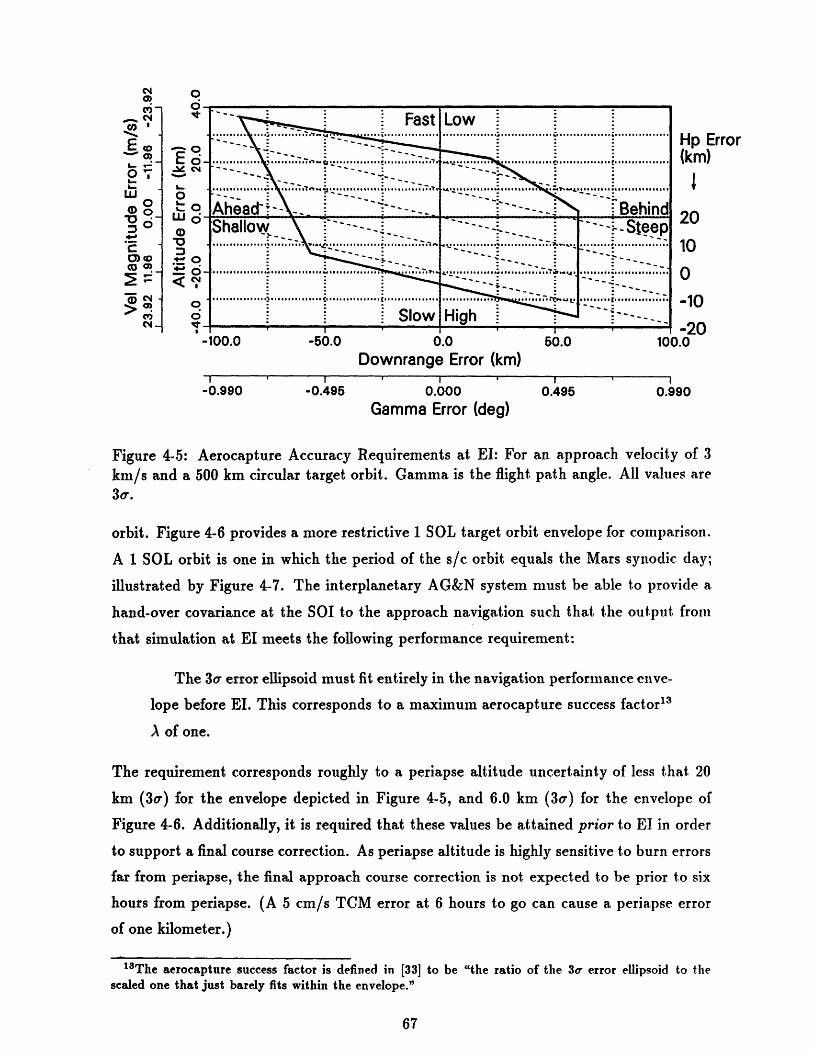
Fast.. . . . . . ... .. .. .. . .=F

a

........ ....... .........'I.............

........... ......... .. 1 .,

................ ........... ............ C..... .......

Slow

Low

....................... .......

................ ........ ".7... ... ..

A ............... ............. ..

............... . ,,, y, •, :... ,,,,

High

. Beninda-- Steep........ ...................

" " . . . . . .... ..................... .I

-100.0 -50.0 0.0 50.0 101Downrange Error (km)

S,..

-0.990I 1

-0.495 0.000Gamma Error (deg)

I.0.495

Hp Error(km)

I20

10

0

-10-20

0.0

0.990

Figure 4-5: Aerocapture Accuracy Requirements at EI: For an approach velocity of 3km/s and a 500 km circular target orbit. Gamma is the flight path angle. All values are3o.

orbit. Figure 4-6 provides a more restrictive 1 SOL target orbit envelope for comparison.

A 1 SOL orbit is one in which the period of the s/c orbit equals the Mars synodic day;

illustrated by Figure 4-7. The interplanetary AG&N system must be able to provide a

hand-over covariance at the SOI to the approach navigation such that the output from

that simulation at El meets the following performance requirement:

The 3a error ellipsoid must fit entirely in the navigation performance enve-

lope before EI. This corresponds to a maximum aerocapture success factor'3

A of one.

The requirement corresponds roughly to a periapse altitude uncertainty of less that 20

km (3a) for the envelope depicted in Figure 4-5, and 6.0 km (3u) for the envelope of

Figure 4-6. Additionally, it is required that these values be attained prior to El in order

to support a final course correction. As periapse altitude is highly sensitive to burn errors

far from periapse, the final approach course correction is not expected to be prior to six

hours from periapse. (A 5 cm/s TCM error at 6 hours to go can cause a periapse error

of one kilometer.)

x'The aerocapture success factor is defined in [33] to be "the ratio of the 3o- error ellipsoid to thescaled one that just barely fits within the envelope."

................. • .......... ,..':,•,

,

7

°r

--·

.. Fast Low

9 Ahead-: Behind

Shalllow - . - SteepSh o ............ ........ .............o -... ·............. .. l... ... . .................. ...... . . ... ......... ....... . .. ... ..............

................ ... ....................... ... ...............

i Slow High-100.0 -50.0 0.0 50.0 10(

Downrange Error (km)• .......

-0.495 0.000Gamma Error (deg)

0.495

Hp Error(km)

20

10

0-10

-200.0

0.990

Figure 4-6: Aerocapture Accuracy Requirements at EI: For ankm/s and a 1 SOL target orbit. Gamma is the flight path angle.

s/c

approach velocity of 3All values are 3oa.

To Sun

Figure 4-7: Cartoon of a 1 SOL Orbit: This elliptical orbit is designed so that an objecton the surface of the planet is observed under the same lighting conditions on each orbitat periapse, but from a slightly different direction. It is also possible to have rationalmultiples of this orbit (i. e. 1/3, 1/5, 1/7 ... SOL orbits).

68

-0.990

Since it will be shown that for reasonable guidance schemes the guidance accuracy

nearly matches the navigation accuracy, the above requirements also apply to guidance

performance. However, as guidance "performance" also includes total fuel cost, the

remaining system requirement is roughly defined as maintaining the total Avt under 50

m/s.

4.3 Simulation Results & Analysis

This section is divided into two portions: interplanetary autonomous navigation (and

guidance), and Mars approach navigation. The former presents the performance of the

baseline AG&N system described in this thesis. The second portion uses the simulator

developed and tested in [33] to continue the navigation down from the SOI to El in order

to fully assess the performance of the prior interplanetary navigation.

4.3.1 Interplanetary Navigation

The following plots present the performance of the baseline AG&N simulation. Specif-

ically they show the effects of autonomous interplanetary navigation measurements on

the uncertainties and dispersions of the s/c state. Figures 4-8 and 4-9 show the current

position uncertainties in the Mars line-of-sight (LOS) and sun-centered local-vertical, lo-

cal horizontal (LVLH) coordinate systems, as defined in Figure 4-10 (these frames alignl4

near the end of the transfer). The LVLH x, y, and z components are also known as the

downtrack, vertical (track), and crosstrack components, respectively. These figures can

be compared against Figure 4-11 which provides a example of what would happen if no

navigation were performed during the mission.

The initial "hump" seen in Figures 4-8 and 4-9 is due to initial conditions (particularly

velocity IC's) and the middle "hump" is due to the s/c remoteness from any planet,resulting in relatively poor measurements. It is interesting to note that the dynamics for

the baseline Hohmann mission first increase the out-of-plane uncertainties but then drive

them back down. This is a direct consequence of having a mission duration of exactly

one half an orbit about the Sun.

It is useful to compare the errors in these systems to determine the regions where

"4Actually, 180* rotated about the z axis.

O0

O-

O 0-

CO-

0-

Qoo

00.

300.0 260.0 200.0 150.0 100.0 50.0 0.0Time to Encounter (Days)

Figure 4-8: Current RMS Position Uncertainties in Mars LOS Coordinates: Baselinecase. The inclusion of Deimos measurements causes a slight jump in the errors and ismarked with a "D".

o

W

Eo.

E0.r 00-

00

C;

to-OIto0*00Q0-C0

0.60-

0

0.


Figure 4-9: Current RMS Position Uncertainties in LVLH Coordinates: Baseline Case.The inclusion of Deimos measurements causes a slight jump in the errors and is markedwith a "D". Final values for the x,y,z components are: 11.93, 235.75, and 11.74 kin. Thefinal LOS values of the previous figure are approximately the same.

A Along LOS UncertaintiesV In Plane Perpendicular Uncertaintieso Out of Plane Uncertainties

A (x) Downtrack UncertaintiesV (y) Vertical Uncertainties (radial)o (z) Crosstrack Uncertainties

A

....................

~~~D....... . .. . .. .. .. ......

.....................

.....................

.. ........ ...... .

XLVLHOrbit of Mars\1I

ytosPlane Perpendicular)

Ktos (Along LOS)

44

Path of S/C

Figure 4-10: LOS and LVLH Coordinate Definitions: Travel is counterclockwise. They component of the LVLH frame is parallel with the position vector of the s/c. The xcomponent of the LOS frame is parallel with the Mars relative position vector of the s/c.The z components of each system are out of the plane of the paper (angular momentumndirection).The LVLH x,y, and z components are also known as the downtrack, vertical(track), and crosstrack components, respectively

200.0 150.0 1

Time to Encounter (Days)00.0 50.0

Figure 4-11: RMS Position Uncertainties in LVLH Coordinates: No Navigation. Clearly,the errors rise to a point where linearity is in question. Note that if guidance does notcorrect for dispersions, then the actual state of the craft will deviate from the nominalin a like fashion.

* (x) Downtrack Uncertainties* (y) Vertical Uncertainties (radial)S(z) Crosatrack Uncertainties

..:.. ..................... ............ ......

qr Id

X

E

oI-0

a-0•

300.0 250.0%

........................... ...................... ..... .................. ......... .............. ............. ............. . ............

................. ........................ .............. .............................. ... .............. ........ ·. · ···..·.· ·.....

I - 1I1

"geometry" and "dynamics" play important roles in the decreasing or increasing the

uncertainties. Good geometry means that the orientation of the s/c and planet(s) is

favorable for navigational measurements to reduce the position uncertainties. The Mars

line-of-sight (LOS) frame best shows the effects of Mars measurements. Geometry effects

are best seen in a LOS frame. The effects of sun-centered, two-body dynamics on the

covariance are best seen with the aid of a local-vertical, local-horizontal (LVLH) frame.

The concept of geometry is important in interpreting Figure 4-8. Geometry and

instrument accuracy largely control the degree of accuracy that optical navigation is

able to achieve. The overall measurement accuracy is proportional to the star tracker

instrument accuracy and inversely proportional to the distance to the observed near body

(see Equation 2.55 on page 26). Figure 4-12 shows the range to each planet as a function

of time on the Hohmann path. Figure 4-12 also shows the LOS rates for both Earth and

Mars throughout the mission. Three important points are exhibited in the figure:

1. As expected for an intercept-type trajectory, the LOS rate (angular rate of LOS

direction) of Mars approaches zero at the encounter as may be seen in Figures 4-12

and 4-13.

2. The LOS rate for the Earth is relatively large at the end of the transfer, making

Earth measurements a possibly significant (see Chapter 5) source of information.

The effect is moderated however by the increasing distance (optical lever arm) to

the Earth.

3. A zone exists where both LOS rates are very low and little information is expected

to be gathered by navigation. Indeed, this time correlates well with the second

"hump" in Figures 4-8 and 4-9.

As is seen in Figure 4-8, optical data provides information about the position com-

ponents of the s/c perpendicular to the line-of-sight to the planet, but little information

along the LOS direction. However, once the measurement(s) has been taken at a par-

ticular point, no further state information can be gathered until the geometry changes

due to dynamics"5 . The measurement range must change and/or the line-of-sight to the

planet must change. Since correlations between the components exist, the more effective

15 However, many (nearly) simultaneous measurements would of course make it possible to reduce theinstrument bias covariance.

O

0

4-

o

oi00

4-

0;

Time to Go (days)

r

-o

4-.o

C)(U

00)4-,

coerr"

C,0

.0

Time to Go (days)

Figure 4-12: Planetary Distances and LOS Rates for the Hohmann Transfer.

-2.5 -2 -1.5 -1 -0.5 0

Distances in km xO10

Figure 4-13: Final Approach for the Hohmann Transfer: LOS spacing of 5.18 days.

.oý.w

way to reduce the error is for the line-of-sight to change"s . The rate at which the line-

of-sight changes is thus another important guide to interpreting the performance of the

interplanetary navigation.

Optical accuracy is also dependent on effective centroiding of the bodies which is

also a function of range (see Equation 2.57 on page 2.57) as well as angular diameter.

Figure 4-14 shows the angular diameters of both Earth and Mars as a function of time.

Figure 4-15 shows two things. First, although the Deimos centroid bias is high (10%),

its angular size is quite small (angular size at SOI is 10 sli). Thus the measurement

accuracy is not significantly affected until only a few days from Mars. Second, the Mars-

Deimos lever arm is a full degree at 15 days to SOI and rapidly growing. This suggests

that Deimos should be able to provide some significant information through its geometry

variation. The effect is detailed further in the next chapter.

Having described the measurement effects on the current performance, it is desirable

to know the measurement effects on the final state and the performance figures-of-merit.

Figure 4-16 shows the current predicted uncertainties at the Mars SOI as a function of

time to encounter. This view of the navigational performance is instructive since it shows

the best currently attainable hand-over accuracy of the approach simulation. It is also

instructive to plot the position performance at entry interface (EI), as does the approach

navigation. However, due to a rapid change in the orientation of the error ellipsoid wrt

the LOS frame just prior to periapse"7 , plotting the projected El errors in an LOS frame

is not particularly helpful'.

An even better illustration is made by dropping the out-of-plane component entirely

and displaying the 2-D error ellipsoid cross-section in the LOS frame during the final

approach. Figure 4-17 depicts the ellipsoids where it is clear that the Mars/Deimos

measurements are rapidly reducing the in-plane perpendicular component while Earth

measurements and correlations help reduce the LOS component. The LOS error is much

larger than the other (two) component(s). Fortunately, the LOS error does not strongly

influence the periapse altitude error, the important aerocapture performance parameter.

Figure 4-18 shows the final error ellipsoid at the SOI as well as after propagating it

1'lndeed, the only way the LOS error component is reduced by optical measurements of a single nearbody is through correlations.

"lThe "curved" portion of the approach hyperbola.'8 Instead, an LVLH representation would be more informative. But just as an LOS representation

does not display useful information near the planet, an LVLH representation does not display well themeasurement effects during the interplanetary phase.

1600

1400

1200

1000

800

600

400

200

50 100 150

Time to Go (days)

200 250

Figure 4-14: Optical Angular Diameters of the Planets with Inset Magnification:Earth = solid, Mars = dashed.

0 50 100 150

Time to Go (days)

200 250 300

Figure 4-15: Optical AngularDeimos = dashed, Mars-Deimos

Diameters with InsetDistance = dot-dash.

Magnification: Mars = solid,

I • I

300I0 - -- - .---------- ,,--W,

k I

--

40

30 i i .... i........................ ......... . ...

- E

.... : .................. .... :-"............. o,,. - ...

so 100 1S0 2O 250 300-~

`~~~i----------------- _~_

0

00E.W..0to

01WC

0

00.c-O

O

n

v

Time to Encounter (Days)

Figure 4-16: SOI RMS Position Uncertainties in Mars LOS coordinates: At day 200 thescale is changed for clarity (right-hand vertical axis). The "D" indicates the bending inthe curves caused by the inclusion of Deimos measurements. Compare with Figure 4-8

EI...

0.LLICoL

(1)0)CtDco

C

-1800.0 -900.0 0.0 900.0 1800.0Along LOS Error (km)

Figure 4-17: Position Error Ellipsoid Cross-Section in the Mars LOS Frame on Days:200, 208, 216, 224, 232, 240, 248, 256. The direction to Mars is indicated by the solidarrow, and the direction to Earth is indicated by the open arrows at each date.

0Ci0-,1.

-.OEo6~~0-(NL-

O0

L

-cooI..

C

3o0

oat

-600.0 -300.0 0.0 300.0 600.0(1h) Radial Error (km)

Figure 4-18: RMS Position Error Ellipsoids at the SOI, at EI, and at Periapse: Theparameters for the ellipse at the SOI are: a = 235.75 kin, b = 11.60 kin, and -89.32".The parameters for the second ellipse are: a = 495.75 kin, b = 9.81 kin, and -11.11.The parameters for the ellipse at periapse are: a = 501.95 km, b = 10.24 km, and -0.15".

down to El and periapse. The semi-major and semi-minor axes as well as the rotation

of the major axis about the LVLH frame are a, b, 0, respectively. Figure 4-19 shows

that the ellipse remains somewhat aligned with the trajectory in the absence of mea-

surements and that the component of the ellipse perpendicular to the trajectory remains

very nearly constant while the other component gets "smeared out" along the trajectory.

The error component perpendicular to the trajectory is, to a good approximation (see

Equation 3.37), equivalent to the periapse error.

Hyerbolic Aworoach Tralectory

Figure 4-19: Effect of Dynamics on Errors With No Navigation During Mars Approach

The actual propagated periapse and inclination errors are given in Figure 4-20. These

77

I l

.................. i................. ................. .................

00


Figure 4-20: RMS Periapse Altitude and Inclination Uncertainties: SOI Final values of10.3227 km and 0.1054 degrees respectively. Again, the "D" marks the noticeable effectof including Deimos measurements.

values are valid not only at the SOI, but at EI and periapse as well because of the smearing

effect previously described. The errors prior to day 134 grow to be as large as 39,800

km and 7980 at injection. These large values are well outside the linear assumption and

are not shown since they are statistical nonsense; a 1000 km error for a 125 km nominal

entry interface altitude could well mean the s/c is below the planet surface.

Guidance Effects

The effect of course corrections on the navigational accuracy can be seen by comparing

Figures 4-16 and 4-21. Figure 4-21 shows the position accuracies when no guidance is

implemented in the simulation. The curvature of the position accuracy plot has hardly

changed. However, the difference can be seen in the final error values of 235.75 km versus

187.52 km, respectively, for the LOS components. To a certain degree, then, the accuracy

of interplanetary navigation is independent of the guidance accuracyl 9 . The converse is

in no way true.

Figure 4-22 shows the velocity uncertainties for the baseline case as a function of time.

The effects of the TCM's cannot be readily seen. However, if the velocity uncertainties

t 9Validating an assumption of Lawden's from the end of Chapter 3.


Figure 4-21: SOI RMS Position Uncertainties in Mars LOS coordinates: Baseline simu-lation without course corrections. Final z, y, and z values: 11.44, 187.52, and 11.36 kin,respectively. The final periapse altitude error for this case is 9.7746 km (lo).

ol'

0~ oEz

o

0co

>0-0'C

000.o co>o~

'-40fi

300.0 250.0 200.0 160.0 1Time to Encounter (Days)

100.0 50.0

Figure 4-22: Current RMSand z values: 1.796, 1.814,

Velocity Uncertainties in Mars LVLII Coordinates: Final x, y,and 1.779 cm/s, respectively.

I (x) Downtrack UncertaintiesS V (y) Vertical Uncertainties (radial)o (z) Crosstrack Uncertainties

',~-c ~

-- ~---- -- --

..................... · · ·

at the SOI are plotted (see Figure 4-23) the errors in measuring the last two burns

are noticeable. This is guidance's effect on navigation. The effects of the TCM's are

more dramatically shown by the periapse parameter dispersions in Figure 4-24. It is

here that the combined effects of navigation accuracy and burn execution accuracy on

guidance performance can be seen. For example, if the last two corrections were not

implemented, the delivered (actual) periapse altitude accuracy would be approximately

950 kilometers (lo) and clearly unacceptable. Each "jump" corresponds to one of the pre-

assigned TCM's. Table 4.5 gives the rms burn size and uncertainty for each correction.

In Chapter 3 it was seen that the navigation accuracy determines the absolute guidance

accuracy.

Table 4.5: RMS Course Corrections for the Baseline Run

Referring to Figure 4-8, it is seen that the pre-assigned TCM dates correspond to

certain navigation accuracies. The first TCM, instead of being very close to injection,

occurs just after the "humps" in the position and velocity uncertainties. This fortunate

placement is dependent both on the high initial velocity errors and on the poor navigation

in deep space. If, for example, the velocity errors were not so large, poor deep space

navigation might still provide the accuracy needed to target correctly earlier on in the

mission. The sensitivity analysis in Chapter 5 does not go so far as to vary two parameters

such as initial conditions and course correction schedule at the same time2 .

The second, third, and fourth TCM follow a simpler pattern. Specifically, they are

placed appropriately to enable guidance to correct for terminal errors without waiting

for further navigation improvement. The extra wait is critical as seen in Figure 4-25. A

balance is reached between waiting for the improved navigation accuracy and the fuel

cost which diverges near the end of the trajectory. Kohlhase [17] describes this waiting

period as the available reaction time for a maneuver.

2 0This is an example of the complexity of the TCM scheduling problem as stated in Section 3.6

TCM Day Size (m/s) Uncertainty (m/s)1 77 6.671 0.9802 141 2.209 0.2623 243 2.482 0.2604 256 1.186 1.182Total: 12.5477 2.684

o

300.0 25( 50.0 0.0Time to Encounter (Days)

Figure 4-23: SOI RMS Velocity Uncertainties in Mars LVLH Coordinates: The day ofeach TCM is marked. The final TCM, at zero days to encounter, is not marked. The

final values for this plot are the same as those of the previous plot.

0-7

An Periapse Alt. D0o Inclination Dis;

..... ... ..... .. ..

150.0 12(Time to Encounter (Days)

Figure 4-24: RMS Periapse Altitude and Inclination Dispersions Showing FTOA Tar-geting Accuracy: Only the last three TCM's are shown, though the accuracy of the firstmaneuver are seen at the upper left.

81

a (x) Downtrack Uncertaintiesv (y) Vertical Uncertainties (radial)o (z) Crosstrack Uncertainties

............................................... .

0-gE rd-0

re0)

4-.Coc

4,-

'-4

0·j

0.

........................i

U

0

00

0ado

oo.0

O0O-0o

E

COo C-

nolo

.00-&- o0.C

O0.

|

r

1 4A

L)V_

O

co

E4--.

OO

0


Figure 4-25: FTOA Cost to Correct for LOS Errors (lo): e. g. an in-plane perpendicularerror of 1000 km costs 1.75 m/s to correct at 200 days to go, but costs 2.6 m/s at 50days to go. The inset show a blow-up of the flat portion of the main plot. The linearguidance matrix B is essentially a Lambert solution matrix which, for a Hohmann transfercontains a tra.nsfer pla.ne ambiguity. The plane "chosen" is one which drastically differsin inclination from the nominal path. The difference shows in the large Av requiredof a plane change. The plot has been generated by targeting for the SOI (encounter).Therefore, the infinite values at 0.0 are not shown in the figure.

4.3.2 Mars Approach Navigation

The ultimate measure of the performance of interplanetary AG&N for the baseline case

lies with a successful aerocapture at Mars. Figure 4-5 shows2 1 that a periapse altitude

error lower than approximately 20 km (3o) is required for a successful capture into a

500 km circular target orbit. Further navigation down from the SOI is needed since the

interplanetary performance, as seen in Figure 4-20 has not achieved this level by a factor

of 1.5.

Periapse altitude error more directly controls the error in the final (sub-SOI) TCM

and plays only part of the role in aerocapture success2 2 . Rather, the entire three sigma

error ellipse must fit within the requirements envelope. The FOM describing this feature

21The upper left corner of the requirements box has the lowest (3o) periapse altitude.22Inclination is not a necessary measure of aerocapture success and has been provided in the previous

sections to show that the plane of the aerocapture is controllable.

(A), is approximately 45 times too large at the SOI. This difference provides a stronger

motive for approach navigation.

The nominal relative state vector and error covariance at SOI of the interplanetary

simulation are sufficient to initialize the Mars approach simulation. The values of the

parameters passed to the approach simulation are listed in Table 4.6. A noteworthy

discrepancy exists at hand-over between the two simulations. The interplanetary simula-

tion ends its simulation at the SOI for this trajectory which occurs at approximately 2.3

days from the nominal periapse. The approach simulation, however, is set to begin at

precisely 2.0 days from EI (EI occurs only minutes before periapse) on a slightly different

trajectory with a hyperbolic excess velocity of 3.0 km/s 23. The difference is not expected

to be significant however, as the linear sensitivities about either orbit should be sinmi-

lar. Also the extra 0.3 days of observations do not significantly improve the navigation

performance.

Position (m2 ) Velocity (m2/s2 )5.557e + 10 -7.695e + 08 1.618e + 08 1.810e + 03 1.516e + 03 -1.028e + 02

- 1.407e + 08 -2.232e + 06 -3.072e + 01 3.061e + 01 1.421e + 00- - 1.402e + 08 5.195e + 00 4.431e + 00 7.839e + 01- - - 3.290e - 04 5.115e - 06 -2.631c - 06S- 2.864e - 04 -3.050e - 06S- 3.527e - 04

Table 4.6: Symmetric Inertial Error Covariance and Mars-Relative Inertial State forInitialization of the Mars Approach Simulation

The approach simulator uses optical measurements of Deimos as it's baseline navi-

gation measurement. Radiometric data from a communications (comm) orbiter in syn-

chronous equatorial orbit are also provided in a separate simulator for comparison. A

third simulator that combines both optical and radiometric data is available as well.

These three simulators include in their covariance, states for the position and velocity

2'The interplanetary trajectory has a Mars-relative hyperbolic excess velocity of 2.9 km/s.

Relative Position (km) Relative Velocity (m/s)x -5.7723240e + 05 2.5688409e + 03y -1.6745310e + 00 -2.3651928e + 01z 1.1012889e - 09 2.3659641e + 01

error of Deimos, and a Mars gravitational parameter error in addition to the state of the

interplanetary approach vehicle. Additional states are for the comm orbiter position and

velocity are also used for the radiometric case.

Figure 4-26 shows the evolution of the two FOM's for the approach simulations. The

periapse error FOM performance for the radiometric case is worse than the optical case

because it cannot sense well the error perpendicular to the s/c - comm orbiter LOS

(nearly equivalent to periapse error) until the LOS changes rapidly near EI. Conversely,

the A FOM performance for the optical case is worse than the radiometric case because

it cannot sense well the s/c - Deimos LOS error component.

0 1.4 - 0

2 cli

0LL 0

O0o04,

0

,)(0I..(0-000

0,

48.0 36.0 24.0 12.0 0.0 48.0 38.0 24.0 12.0 0.0Time to El (hr) Time to El (hr)

Figure 4-26: Baseline Performance for Three Cases of the Approach Simulation: All casesuse the 500 km capture requirements. The final value for the periapse altitude error andA for the optical case are 2.88 km and 0.42.

Figure 4-27 shows the 3o error ellipsoid evolution beginning at 12 hours to entry

interface (EI)24 . It can be seen from Figure 4-28 that the ellipsoid is nearly aligned with

the Mars LOS at 2 hrs from EI. This geometry, due to the additional measurements,

differs from the orientation of Figure 4-19. Not until 2 hrs before entry interface (EI) is a,

successful aerocapture assured (3a ~ 99.73%) for the optical only case. This is the point

at which linear navigation suggests that more measurements are no longer required for

2 4Entry interface with the atmosphere is defined to be 125 km [33].

84

E

(D -C401

c-oacoC

4.00-0

IL

,-s(/)•

bO o

o-

A OpticalV Radio Rangeo Optical+ Range ........... ..

. . . . . .

t OpticalSRadio Range

Optical + Range

L 9 a

..--. .Fast........... ........ ....... .... .........

AheadShallow................,

Si S.....low..Slow

-150.0

Low................ ................ ................ .. .......... ......... .... ..... .... ..... ..... . ... ..... .....

Behind--Steep......

....

...... .

High -- -

0.0Downrange Error (km)

150.0 3C

0

E d--Y co

-2.970 -1.485 0.000Gamma Error (deg)

1.485 2.970

Figure 4-27: Baseline Performance for The Optical Case of the Approach Simulation: 3f"

Ellipsoids at 12, 9, 6, 3, 0 hours before El. The ellipse is contained entirely within the

500 km circular capture orbit requirements box at 2 hours to EI. The ellipsoid at 9 hrs is

set at -12.6 degrees from the LVLH frame and the ellipsoid at El is set at -30.5 degrees.

Periapse

Periapse Uncertainty - ahp

Figure 4-28: Relative Geometry of the Error Ellipsoid for Approach Navigation

85

Hp Error(km)

6030O

-30

-60)0.0

0-

oc

01

-300.0

v Z•E --2

Wr- -.- -1 I • ' ' . .

-

LU lp-ý -

-I-"

6;-9

II

success. Of course, further measurements can only reduce the covariance. By combining

both radiometric and optical types, this level of state knowledge is attained much sooner

at 27.5 hrs to go.

Returning to the optical-only case, the time at which the 3ar periapse altitude error

falls below the required 20 km occurs at 22.0 hrs; well before the A requirement is

attained. This is not true for the radiometric only case. The ability to have accurate

periapse knowledge is important in considering the timing of the final TCM. The sooner

an adequate accuracy is attained, the lower the correctional maneuver costs. Since the

interplanetary guidance has been shown to maintain the s/c close to the nominal, this

TCM is not expected to be large as shown in [33] even as late as six hours before EI.

In fact, the final TCM should be delayed so as to reduce the effects of burn execution

errors so long as the total fuel cost remains low. The 20 km periapse altitude error

"requirement" becomes somewhat less important than the A FOM.

4.3.3 Summary

It has been shown that interplanetary AG&N provides adequate performance for a suc-

cessful aerocapture mission resulting in a 500 km circular orbit about Mars. However,

to arrive at this performance level, many assumptions defining the baseline mission have

been made. Obviously, many, if not all, of the baseline parameters will change during

actual mission design. In order to infer the applicability of interplanetary AG&N to other

missions, Chapter 5 varies the key assumptions and parameters in a sensitivity analysis

of the baseline mission.

Chapter 5

Variational System Performance

and Sensitivity Analysis

The previous chapter discussed the performance for what is thought to be a very rea-

sonable baseline mission. The purpose of this chapter is to ascertain whether or not

that case is overly sensitive to any of the assumptions that define the baseline. This

is accomplished by varying each key parameter in the system, one at a time, and then

comparing the resulting system performances with the nominal results. The parameters

that are to be varied in this sensitivity analysis are listed in Table 4.4 (page 65). Ofthe many possible variations about the baseline, 21 have been chosen and are grouped

into three sections: Navigation Error Source Variations, Environment Variations, and

Guidance Variations.

A detailed analysis similar to that for the baseline run for each variation would be

impractical. Therefore, several key performance quantities for all the variational runs

are tabulated so that, when grouped together, the relative importance of any particular

parameter is apparent. Tables 5.1 and 5.2 summarize the overall performance of inter-planetary navigation and guidance variations while Table 5.3 summarizes the objective

of each case. Table 5.4 describes the approach navigation performance for four of the

variations.

Run DescriDtion:

Baseline

10 Arcsec Star Tracker

2 km, 2 cm/sec InitialCondition (Errors)5% Planet Centroid Bias

2x Process Noise

0.01x Process Noise

No Deimos Measurements

Substitute Deimos for MarsMeasurements at 5 Days to GoDrop Earth Measurementsat 20 Days to Go2x Measurement FrequencyUntil 20 Days to GoMars Observer Orbit

Sprint Orbit

Include Radiometric from Earth

Include Radiometric from Earth(Doppler Only, No Range)Begin Trajectory withRadiometric I.C.'s At 64 Days to Go

LVLH Position Uncertainties (km)& Ellipsoids (km,km,deg)

SOl El at 125 km

x (dt) y (vt) z (ct) x (dt) y (vt) z (ct)a b phi a b phi

11.93 235.73 11.74 486.46 96.03 5.99235.75 11.60 -89.32 495.75 9.81 -11.1122.34 314.22 22.29 650.09 131.42 10.90

314.23 22.29 -89.71 663.00 17.76 -11.3311.78 231.27 11.59 477.28 94.26 5.84

231.28 11.46 -89.33 486.41 9.57 -11.1212.70 289.32 12.45 5986.18 118.02 6.86

289.34 12.15 -89.27 607.65 11.22 -11.1512.13 255.04 11.89 526.19 103.41 6.09

255.06 11.66 -89.25 536.16 9.94 -11.0711.72 212.54 11.59 438.73 87.20 5.88

212.55 11.52 -89.42 447.21 9.64 -11.18

495.98 31.09

116.6150.43

Ia F~68.40

237.79237.78

68.3768.37

-89.52499.37508.67515.07524.42459.54468.27518.87527.81646.30661.03145.16148.19198.46202.5585.6187.48

6.23-10.97

9.05-10.84

5.76-11.08

6.39-10.56

10.66-12.12

5.84-11.63

5.87-11.54

5.73-11.94

13.29242.7520.06

251.4311.58

222.7313.02

264.4314.14

456.1111.4169.0911.4794.6911.3439.81

242.7112.49

251.3418.87

222.7111.22

264.3210.44

456.0712.5769.0911.4194.6811.4739.8011.33

13.03-88.93

20.10-88.4411.39

-89.2611.97

-88.3114.74

-89.1911.42

-89.8511.4889.9311.33

-89.21

97.3410.0899.6314.3690.499.43

97.108.87

139.3011.8231.28

9.4841.59

9.5220.27

9.32

No Burn Execution Errors 11.44 187.52 11.36 387.43 - 77.67 5.60187.52 11.34 -89.55 395.03 9.15 -11.26

VTOA, Last Burn 11.93 235.73 11.74 486.46 96.03 5.99(Time Deviation: 0.023 Hours) 235.75 11.60 -89.32 495.75 9.81 -11.11Guide for Periapse & Inc., Last Burn 11.93 235.73 11.74 486.46 96.03 5.99(Time Deviation: 0.347 Hours) 235.75 11.60 -89.32 495.75 9.81 -11.11Guide for Periapse Only, Last Burn 11.93 235.73 11.74 486.46 96.03 5.99

235.75 11.60 -89.32 495.75 9.81 -11.11VTOA All 4 Burns 11.93 235.73 11.74 486.46 96.03 5.99(Total Time Deviation: 8.925 Hours) 235.75 11.60 -89.32 495.75 9.81 -11.113 Burn, Correction Schedule 11.69 231.96 11.52 478.92 94.85 5.74(30, 55, 100 %) 231.97 11.42 -89.38 488.13 9.40 -11.155 Burn, Correction Schedule 11.93 235.88 11.74 486.77 96.09 5.99(5, 30, 55, 95, 100 %) 235.90 11.60 -89.32 496.07 9.81 -11.11

Table 5.1: Performance for Variations About the Baseline Scenario at the SOI, EI, andPeriapse (Part 1): Each Variation is numbered 2 through 22. The first grouping (1-6)varies navigational error sources. The second group (7-15) varies the measurement envi-

ronment. The last group (16-22) varies the guidance errors, scheme, and schedule. All

values are lor. Uncertainties: "dt": downtrack, "vt": vertical (radial), "ct": crosstrack.

495.98507.00

31.09-12.031

."rL,3.•.I iv.v -v. I I I I .. UbU

515.43 53.56 24.90 53.558 0.547 53.610 0.547 12.513515.55 52.42 -1.23 1.272514.73 10.53 4.99 10.526 0.105 10.815 0.109 12.572514.73 10.53 0.00 1.218530.36 15.06 7.25 15.057 0.154 15.365 0.157 12.839530.36 15.01 0.13 1.263474.07 9.89 4.62 9.890 0.101 10.101 0.104 11.468474.07 9.84 -0.12 1.118532.85 10.39 5.18 10.396 0.107 10.509 0.109 10.240532.87 9.29 0.50 1.371666.30 12.31 9.70 12.310 0.153 16.215 0.206 18.345666.30 12.31 -0.03 3.987150.38 10.06 4.68 10.064 0.103 10.139 0.104 7.542150.40 9.88 -0.73 0.359205.47 10.16 4.71 10.165 0.104 10.256 0.105 7.839205.48 9.92 -0.62 0.48588.91 9.86 4.59 9.856 0.101 9.937 0.101 1.69688.93 9.69 -1.116 0.222

400.23 9.77 4.48 9.775 0.100 9.775 0.101 12.202400.24 9.54 -0.30 0.940501.95 10.32 4.80 10.323 0.105 10.426 0.107 11.809501.95 10.24 -0.15 0.085501.95 10.32 4.80 10.323 0.105 10.425 0.107 11.811501.95 10.24 -0.15 0.086501.95 10.32 4.80 10.323 0.105 10.441 0.107 11.741501.95 10.24 -0.15 0.072501.95 10.32 4.80 10.323 0.105 10.418 0.108 5.383501.95 10.24 -0.15 0.085494.32 9.95 4.60 9.948 0.102 33.026 0.343 24.471494.32 9.82 -0.19 1.163502.27 10.32 4.80 10.323 0.105 10.613 0.109 12.702502.27 10.24 -0.15 1.183

Table 5.2: Performance for Variations About the Baseline Scenario at the SOI, EI, andPeriapse (Part 2): Each Variation is numbered 2 through 22. The first grouping (1-6)varies navigational error sources. The second group (7-15) varies the measurement envi-ronment. The last group (16-22) varies the guidance errors, scheme, and schedule. Allvalues are lar. Uncertainties: "dt": downtrack, "vt": vertical (radial), "ct": crosstrack.

LVLH Position Uncertainties (km) Parameter Errors at SOl, El, Periapse Total AV& Ellipsoids (km,km,deg) and Last Burnd....... •i al......t.....................(............ .Un.a.ity

x (dt) y (vt) z (ct) alt. (km) incl. (deg) alt. (km) incl. (deg) (m/s)a b phiI•////////• ///////• •///////• •////,•,•/////-- --------------------/////////

501.95 10.32 4.80 10.323 0.105 10.613 0.109 12.548501.95 10.24 -0.15 1.182671.93 19.04 8.73 19.038 0.194 19.420 0.199 16.261671.94 18.52 -0.38 1.577492.51 10.08 4.68 10.078 0.103 10.343 0.106 2.286492.51 9.99 -0.15 - 1.160615.35 11.88 5.50 11.879 0.121 12.471 0.130 17.856615.35 11.71 -0.18 1 1.447542.77 10.43 4.88 10.429 0.107 10.750 0.111 12.652542.77 10.38 -0.10 1.280452.93 10.21 4.71 10.206 0.104 10.464 0.108 12.4344593) 0 100 i -021 1 06 A '

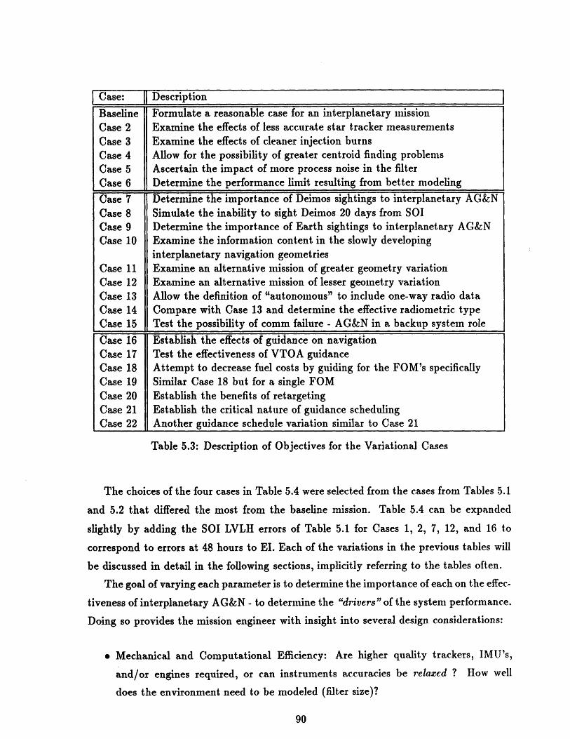
Case: DescriptionBaseline Formulate a reasonable case for an interplanetary missionCase 2 Examine the effects of less accurate star tracker measurementsCase 3 Examine the effects of cleaner injection burnsCase 4 Allow for the possibility of greater centroid finding problemsCase 5 Ascertain the impact of more process noise in the filterCase 6 Determine the performance limit resulting from better modeling

Case 7 Determine the importance of Deimos sightings to interplanetary AG&NCase 8 Simulate the inability to sight Deimos 20 days from SOICase 9 Determine the importance of Earth sightings to interplanetary AG&NCase 10 Examine the information content in the slowly developing

interplanetary navigation geometriesCase 11 Examine an alternative mission of greater geometry variationCase 12 Examine an alternative mission of lesser geometry variationCase 13 Allow the definition of "autonomous" to include one-way radio dataCase 14 Compare with Case 13 and determine the effective radiometric typeCase 15 Test the possibility of comm failure - AG&N in a backup system role

Case 16 Establish the effects of guidance on navigationCase 17 Test the effectiveness of VTOA guidanceCase 18 Attempt to decrease fuel costs by guiding for the FOM's specificallyCase 19 Similar Case 18 but for a single FOMCase 20 Establish the benefits of retargetingCase 21 Establish the critical nature of guidance schedulingCase 22 Another guidance schedule variation similar to Case 21

Table 5.3: Description of Objectives for the Variational Cases

The choices of the four cases in Table 5.4 were selected from the cases from Tables .5.1

and 5.2 that differed the most from the baseline mission. Table 5.4 can be expanded

slightly by adding the SOI LVLH errors of Table 5.1 for Cases 1, 2, 7, 12, and 16 to

correspond to errors at 48 hours to EI. Each of the variations in the previous tables will

be discussed in detail in the following sections, implicitly referring to the tables often.

The goal of varying each parameter is to determine the importance of each on the effec-

tiveness of interplanetary AG&N - to determine the "drivers" of the system performance.

Doing so provides the mission engineer with insight into several design considerations:

* Mechanical and Computational Efficiency: Are higher quality trackers, IMU's,

and/or engines required, or can instruments accuracies be relaxed ? How well

does the environment need to be modeled (filter size)?

* Mission Design: Optimal scheduling of measurement types and dates, and schedul-

ing of TCM types and dates.

More detailed and/or specific case studies can be formulated more efficiently given

insight into the interplanetary AG&N drivers. Lastly, the obvious drivers are grouped

into dominant navigation parameters that minimize the SOI position uncertainty. The

velocity uncertainties are not explicitly important though they do implicitly reveal them-

selves through the periapse parameter uncertainties. Dominant guidance drivers fall into

two groups: parameters that minimize total fuel cost and parameters that minimize the

difference between the periapse parameter uncertainties and dispersions.

Periapse Alt. Error <= 20 km (3 o- ) Figure-of-Merit (FOM) <= 1Variation ............................ at: (hours to El) . at (hours to El)

Optical RadioRangelOpt. & Radio Optical RadioRangeOpt. & RadioBaseline 22.00 6.00 25.50 2.00 6.17 27.50

7 j 15.50 5.17 17.50 2.00 5.33 17.50Case.12 18.00 5.67 23.50 2.00 5.83 25.0

Case 16 24.00 6.33 29.50 2.00 6.67 30.50

X-Y Position Error Ellipsoids @ El wrt LVLH (Optical Approach Navigation Only)Variation: at 24 Hours to El at El

a (km b ........ .. hi(degrees)I a (kmn) b (kin) Jphi(degrees)Baseline 317.22 6.63 -11.29 5.75 2.11 -30.50

Case7 322.82 8.60 -11.46 5.84 2.14 -31.23

Case 16 281.40 6.30 -11.37 5.70 2.07 -30.47

Table 5.4: Approach Navigation Performance for Four Variational Cases: The top tablelists, for four selected variational runs, the times at which the periapse altitude error (30r)dives below 20 km and the aerocapture figure-of-merit (A) dives below 1. As each casemeets these conditions, interplanetary AG&N is deemed successful for these cases. Thelower table, shows that the approach navigation reduces the SOI errors in such a way tomake the variational cases indistinguishable at EI. This is largely due to the increasingstrength of Deimos measurements as the s/c approaches Mars. Without explicitly simu-lating the 1 SOL capture orbit, it can also be seen that the ellipsoid at El just fits insidethe second requirements box of Figure 4-7 on page 68, also indicating success.

5.1 Navigational Sensitivities to Error Sources

Errors enter the navigation portion of the analysis through the finite resolution of the star

tracker, IMU drift, the planet centroiding problem, initial conditions (errors), and process

noise. These errors drive the entire navigation problem away from the deterministic case

(perfect world). This section describes the navigation performance of several error source

variations. The errors can be roughly grouped as "mechanical" errors - errors inherent in

the present navigation sensor technology; "environmental" - those errors which cannot

be controlled, only modeled; and "filter" - errors artificially introduced by the estimation

process. These groupings help clarify the analysis.

5.1.1 Mechanical Error Sources

Referring to the variational results, it is clear that the star tracker accuracy has the

greatest influence on navigation performance, while injection (a priori) velocity errors

have the greatest influence on total fuel cost. Case 2 changes the star tracker measurement

accuracy to 10 0s (1)o from 5 s . The angle bias mean value is also changed to 10 sec.

It is seen that the periapse parameter uncertainties are nearly doubled. The relationship

between the non-LOS error components and the star tracker accuracy is nearly linear.

The fact that this relationship does not hold for the LOS component shows that state

errors along the LOS are driven by correlations more than by Earth measurements. Note

also that a significant 30% increase in fuel cost is incurred by doubling the measurement

error.

The approach navigation performance for this important case is presented in Ta-

ble 5.41 and Figure 5-1. The periapse altitude uncertainties are displaced upwards from

those in Figure 4-26 on page 84 for the baseline case by a factor of two. The aerocapture

success FOM, on the other hand behaves in a similar manner.

Case 3 supposes that the injection velocity errors are smaller by a factor of 100 (more

precise engine control is available), reducing both uncertainty and dispersion covariance

initial conditions. If a post-injection hand-off covariance is minimized from navigation

information from the GPS system with the original injection velocity errors is assumed,

then only the uncertainty portion of the covariance would be reduced. Notice tha.t the

1Note that due to the optimal Deimos measurement geometry assumed by the approach simulator,and an IMU alignment at 2 hrs to go, all the variations produce a 2 hrs A crossing.

0LL

CL00

0Ur,a.0)0,0I.0o

Time to El (hr) Time to El (hr)

Figure 5-1: Approach Navigation Figures-of-Merit for Variational Case 2

navigation performance (Figure 5-1) is changed very little from the baseline (Figure 4-

26). As shown by Figures 5-2 and 5-3 2, deep-space navigation has no real ability to

reduce velocity errors that are already below the attainable level of optical interplanetary-

type measurements. Additionally, since velocity errors largely drive position errors, the

position errors also remain small enough that Mars measurements alone are able to reduce

the errors. Dropping the Earth measurements entirely for this case may have the same

result.3 Navigation performance is NOT, then, driven by initial condition errors.

Of course, with much more accurate mid-course state information, the scheduled

TCM's correct for smaller present errors through smaller sized burns (and smaller asso-

ciated execution errors). The guidance also targets more accurately and thereby reduces

the size of all subsequent TOM's. These combined effects result in a drastic cost reduction

for the mission from 12.5477 to 2.2860 m/s, a savings of 82%.

2To compare these figures, refer to Figures 4-8 and 4-22 on pages 70 and 79.SDropping Earth measurements when the a priori errors are large, however, allows the errors to grow

enough that Mars measurements cannot fully reduce the errors to the baseline level.

N

07E0

o0C 0-u0

00

0-

oOo

I.0 150.0 1


Figure 5-2:values are:

0C4

U)

E6-ica0

00

c

4.2

0000C

.ao*0

> &

00

(lo) LOS Position Uncertainties for Variational11.78, 231.27, and 11.59 km respectively.

Case 3: Final x,y, and z

.0 160.0 1


Figure 5-3: (lr) LVLH Velocity Uncertainties for Variational Case 3: Final x, y, and zvalues are: 1.72, 1.81, 1.71 cm/s respectively. Effects of the four TCM's are marked. Thefourth TCM occurs at zero days to encounter.

94

a Along LOS Uncertaintiesv In Plane Perpendicular Uncertainties0 Out of Plane Uncertainties

~1~

300.0 200. I00.0 50.0 0.0

A (x) Downtrack UncertaintiesV (y) Vertical Uncertainties (radial)0 (z) Crosstrack Uncertainties

................... ....................... i..... ............. ................ ................................ ........................

I3300.0 260.0 200. 100.0 50.0

I I, _. .

1

.................... ........................ ........................ ........................ ........... ..... ' ' ' ' '

........ ................ .. .............. ................ ..... .. . .. ..... . ..... ........

I-250.0

.................

.......... . ........

-r

5.1.2 Environmental and Filter Error Sources

Centroiding errors result from both filter and environmental factors. The filter con-

tributes to this error source through limitations in the centroiding algorithm (onboard

software). The environment component of this error source results from the irregular

physical shapes of the planets and moons, and also from the surface albedo variations.

The 1% (la) value used for the planetary centroid bias has been increased to 5% for

Case 4 (although the centroid bias for Deimos is kept at 10%) to test for sensitivity to

that assumption. Of the error sources, centroid errors have the second largest effect on

both navigational and guidance performance: 15% increase in periapse altitude error and

42% increased total fuel cost.

Process noise (PN) is similar to centroid errors in that it has both environmental

and filter error source qualities. PN is included to account for the environmental effects

of solar wind and radiation pressure variations and errors, gravitational constant error,

and planet ephemerides errors and the inadequate modeling of these states in the filter.

Cases 5 and 6 vary the process noise value used for state propagation. By comparing

Case 6 and the baseline run, it is seen that PN drives the out-of-plane error during the

interplanetary phase, and the downtrack error during the hyperbolic approach. However,

PN is not considered an overall major error source for the navigation system.

5.2 Sensitivities to the Environment

The second group of variational test cases listed in Tables 5.1 and 5.2 illustrate how the

baseline navigation system reacts to optical measurement scheduling, and to changes in

the nominal trajectory. Cases 7 through 10 modify the optical measurement body and the

measurement frequency. Cases 11 and 12 modify the mission trajectory. Cases 13 and 14

include radiometric measurement types, and Case 15 alters the simulation starting point

along the trajectory. These cases test the AG&N performance sensitivity to controllable

parameters.

5.2.1 Modified Measurement Schedule

Case 7 and 8

Deimos measurements have a strong effect on the periapse altitude knowledge generated

by the interplanetary AG&N system. As seen by the delayed FOM crossings in Table 5.4

and Figure 5-4, the absence of Deimos measurements also has a significant impact on the

(optical) final approach performance. The effect is seen best in the disparity between the

downtrack position error component at the SOI of Case 7 and the baseline case; 68.40

km and 11.93 km respectively. As shown in the previous chapter, the downtrack error

component most directly reflects the periapse error. Note also that the vertical error has

increased as well which is probably best explained by the fact that during the process

of switching from Mars to Deimos measurements, the angle bias and Mars centroid bias

correlations with other states are zeroed. Since the Mars LOS estimation is primarily

accomplished through correlations, there is a brief period which is needed to build these

correlations back up so that the LOS errors can again be estimated.

48.0 38.0 24.0Time to El (hr)

-712.0 48.0 36.0 24.0

Time to El (hr)


It is interesting to note from Case 8 that if Deimos is picked up at five (rather than 20)

days prior to SOI, accuracies nearly as good as the baseline result. This behavior should

actually be expected since even Case 7 (Deimos picked up at SOI - approximately two

days from EI) yields favorable approach performance. Note that the vertical accuracies

are slightly worse for the same reason given above for Case 7.

96

a OpticalV Radio Range0 Optical + Range

-.-. ..........

. . . . .. . . . . .

0O

o-

0I._

o -

o-

a

ECcoC

co.a

(D0

16ý00,

03

12.0 0.0-ISI I r

0.0

Case 9

In order to understand the role of the launch planet during optical measurements, Case 9

ceases Earth measurements with 20 days before encounter although Deimos is still substi-tuted for Mars. Note that all three of the SOI LVLH error components have increased as

has the periapse error. By referring to the Earth LOS vectors in Figure 4-17 on page 76,

it is seen that the Earth does help reduce the Mars LOS error component near the end

of the trajectory. Since the errors are less than those of Case 2, a successful aerocapture

can be expected.

This explanation for the position uncertainty reduction at encounter inadequatelydescribes the effects of Earth measurements on the total AG&N performance. For this

reason, several other simulations were made varying the scheduling of Earth measure-

ments. The results of these variational cases are presented in Table E.1 in Appendix E.

The runs indicate several influences which are described below:

* At least for the current sub-optimal simulator4 , Earth measurements are unneces-

sary from the point of view that only the periapse altitude is the critical parameter.

It is seen that lower h, uncertainties than the baseline case are obtained if Earth

measurements are not utilized during the mission even though the actual multi-

dimensional state error ellipsoid still consistently shrinks with the use of Earth

measurements. This counter intuitive result is probably due to the fact that the

simulator is sub-optimal (see [31]). It seems that the correlations between the

cartesian position components and the velocity components match in such a way

that this one-dimensional "slice" (Sh,) is increased, at least for this particular mis-

sion construction (i. e. consider states, Hohma~nn dynamics, and Earth observation

geometry).

* However, Earth measurements are needed in order to provide guidance accuracy.

To support the first two TCM's that reduce the majority of the dispersion error,Earth measurements must be utilized as they are the best source of navigational

information at the beginning of the mission. Whether or not Earth measurements

are used, the final uncertainties and dispersions are below that of variational Case 2

and 7. Therefore, a successful aerocapture can be expected.

4 Due to the presence of consider states.

* Appropriate deletion of certain Earth measurements during the mission can lead to

nearly the same overall performance as the baseline case. For example, Earth mea-

surements during the final few days significantly reduce the position error ellipsoid

due to the rapidly changing observation geometry while mid-course measurements

add very little information.

The role that the launch planet plays in interplanetary (optical) AG&N is more impor-

tant to guidance efficiency than to navigational performance but can play an extremely

useful navigational role. The example demonstrates the importance of understanding the

purpose and effect of (sub-optimal) consider states and of optimal selection measurements

(see Section 2.4.3).

Case 10

It is always possible to reduce to state errors by taking more measurements. However, in

this case, only slight improvement occurs which is to say that enough measurements are

being taken for simulation purposes. While an actual mission has plenty of time to take

more measurements, the potential improvement would have to be weighed against such

drawbacks as having to power up the IMU s. Case 10 doubles the optical measurement

frequency of Earth and Mars to twice a day for each planet, but only results in the

periapse altitude error decreasing by 4.2% .

5.2.2 Alternate Mission Trajectory

The importance of the nominal mission trajectory is based on the fact that all the sen-

sitivity matrices of the simulation are evaluated on that path. An example of mission

dependence, explained in Section 4.3.1 (see Figure 4-11), is the unique dynamical in-

fluence on the out-of-plane errors for a Hohmann transfer. An obvious variation of the

baseline is to examine a different trajectory. Two trajectories are chosen in order to

capture both greater geometry variations and faster dynamics than the Hohmann path

represents. Both paths are out-bound paths from Earth to Mars. In-bound trajectories

would, however, provide a much greater geometry variation for sightings on the planets,

including Venus.

"Again, the IMU is used as a reference during a measurement for the present measurement set-up.

Case 11

The first mission variation chosen is that of the Mars Observer (see [24]) which begins

on August 20, 1990 and ends on August 12, 1991. The mission initial conditions are

presented in Table 5.5. The planetary initial states are found from actual ephemerides

given by Danby [8]. This trajectory results in a wider geometry variation than the

baseline Hohmann mission (see Figure 5-5). Knowing the almanac ephemerides for the

planets, a Lambert transfer for these dates gives a trajectory with inclination of 2.2840

degrees to the ecliptic and travels through 217.3 degrees of arc. The only significant

simulation result of this variation is that the total fuel cost is 18% less. The navigation

uncertainties are similar to the baseline case. The second trajectory variation has a much

greater effect on the performance of the AG&N system.

Spacecraft:

Earth:

Mars:

Position (km) Velocity (km/s)x 1.26867537e+8 1.65408705e+1y -8.15081199e+7 2.87421708e+1z 1.94646274e+5 -1.32253359e+0x 1.27251706e+8 1.56451191e+1y -8.19623704e+7 2.49334251e+1z 0.Oe+0 0.Oe+0x 2.073009536e+8 -2.42486634e+0y 2.90442755e+7 2.60613684e+1z -4.48132898e+6 6.06243139e-1

Table 5.5: Initial Conditions for the Mars Observer Variation: Inertial Coordinates.

Case 12

The most likely type of manned-mission to Mars will be a "sprint" type trajectory to

minimize the flight duration effects on the crew. The mission start date is March 13, 2016,and the encounter is on August 27, 2016. The mission initial conditions are presented

in Table 5.6. The trajectory, presented in Figure 5-6, is inclined to the ecliptic plane by

2.0850 degrees, and travels through approximately 123.7 degrees of arc.

The SOl crosstrack errors for this case are a significant 93% greater than the baseline

case and the periapse altitude error rises by 19%. Additionally, the total fuel cost in-

creases by 46% - the second largest change of any variational run. This case also exhibited

9

Figure 5-5: Mars Observer Trajectory: x-y Planar Projections. Spacing between points:13.73 days.

the second largest out-of-plane error at periapse (9.7 km (1o)). An approach simulation

was performed for this case resulting in the figures-of-merit histories of Figure 5-7. Again

the approach navigation shows that the variation can be accommodated successfully.

The errors for this case may actually be greater than are presented here due to

the SOI hand-over mismatch between the simulators described in Section 4.3.2. The

sprint trajectory case has a hyperbolic excess velocity of 4.812 km/s which is significantly

different than the approach simulator's assumed 3.0 km/s approach. Thus, the duration

Spacecraft:

Earth:

Mars:

Table 5.6: Initial Conditions for the Sprint Orbit Variation: Inertial Coordinates.

100

Position (km) Velocity (km/s)x -1.47503794e+8 -6.81976416e+0y 1.70638244e+7 -3.16028043e+1z -1.60005580e+5 -1.17463094e+0x -1.47712570e+8 -3.93440258e+0y 1.72216245e+7 -2.97021054e+1z O.Oe+O O.Oe+0Ox -2.13587548e+8 1.19672213e+1y -1.09699480e+8 -1.94786146e+1z 2.96750736e+6 -7.01644095e-1

1.5

0.5

0

-0.5

-1

-1.5

.)

Figure 5-6:days.

Sprint Trajectory: x-y Planar Projections. Spacing between points: 8.35

48.0 36.0 24.0Time to El (hr)

(O(I)a

0j0c0

U)0

a)

0.012.0 48.0 38.0 24.0

Time to El (hr)


101

............ ·~.............

.. .. .. ... .. ... .. .. . ... .. ... .. ... .. ... .. .... ... .. .

·.. ...... .. . ...

& OpticalI Radio Range* Optical + Range .

12.0 0.0

-

-

i'

.A-

................. ................................ ·; ···- · ·- ··.· -... ; .·.. ... .....

........................... .............

-1 I ,-qIF

of the approach is less, the navigational accuracies are reduced, and the linear sensitivities

are different. A better match and further investigation of this case is recommended for

future work.

5.2.3 Inclusion of Radiometric Data

The possibility of receiving 1-way Doppler and ranging information on-board the s/c

by sampling a pure tone or coded pulse sent from Earth must be considered. In the

case of Doppler data, the scheme is simple and would not require a sophisticated system

such as the DSN to emit the tone, and therefore might qualify as an autonomous data

type. Case 13 includes both measurement types, while Case 14 adds only Doppler. The

interplanetary AG&N filter includes range bias and drift states as well as a Doppler bias

state. Modeled as ECRV considered states, their respective la noise values are 1.4 x 10-8

meter per meter of range, 0.003 m/s , and 0.01 m/s (refer to Section 2.5 for citations).

The la bias values are taken to be equal to the noise values.

Both measurement types are quite powerful in reducing the Earth LOS error as shown

in Figures 5-8 and 5-9 where variations using only radiometric measurements are pre-

sented. It is doubtful that these cases could support aerocapture since, upon reaching

Mars, the errors are larger than the optical baseline navigation system. Cases 13 and 14

show that the only significant change in uncertainty accuracy is in the radial direction -

improvements of 71% and 60% respectively. The use of radiometric data does not signifi-

cantly reduce periapse altitude or inclination errors. However, a significant improvement

over the baseline case is seen in fuel cost (nearly a 40% decrease). This drastic change

occurs because the FTOA guidance scheme used has attempted to null all three compo-

nents of the periapse position error which, until now, has contained a large component in

the downtrack direction. A variation left for future study is to apply the third guidance

scheme of Section 3.4 to Case 13. It is expected that the change between that run and

Case 13 will not be as great as the difference between Case 19 and the baseline case.

5.2.4 Backup System Role

Placing this section under the heading "Sensitivities to the Environment" in an attempt to

explain performance sensitivity to a controllable parameter is perhaps strange. However,

communication failure, explored by Case 15, can only be considered "controllable" by

102

O0

E o00

0

Oo0-6

C;0aoS0,0.

300.0 260.0 200.0 160.0o 100.0 6.0 0.oTime to Encounter (Days)

Figure 5-8: RMS Earth-LOS Current Position Uncertainties: Doppler tracking of Earthwithout optical measurements. Note that the LOS system is not wrt Mars, but wrtthe Earth and that no optical measurements are taken. Also note that the out-of-planecomponent is much larger than the two components shown. However, the out-of-planecomponent follows a nearly identical path as the out-of-plane component of the othervariational cases - the out-of-plane component dynamics reduce the error near the end.The final zx,y, and z position errors are 162.70, 234.42, and 113.30 kin, respectively. (Theellipsoid parameters are: a = 268.47 km , b = 96.67 kin, and q = 58.500.) The final z, y,and z velocity errors are 34.24, 1.55, and 37.25 cm/s, respectively (considerably largerthan the baseline final velocity errors). The final periapse altitude and inclination errorsare 93.19 km and 0.951 degrees.

making the comm link more reliable. Case 15 is presented here only to continue the

logical progression of Section 5.2.

The start of Case 15 is at 64 days (1/4 of the transfer time) before the SOI. The a

priori position and velocity covariance is a diagonal matrix with values representative of

Earth radiometric tracking up until that point. The LVLH lo- values are: 40.0,40.0, and

100.0 km position, and 0.005, 0.010, and 0.020 m/s velocity. These figures are taken from

the running values for Case 13, though actual DSN tracking is expected to be somewhat

more accurate. Correlation terms are not included.

The navigational performance at the SOI in this case is similar to the baseline case. Of

course, the fuel cost is much lower since the initial conditions are much smaller. It is left

103

A Along LOS Uncertaintiesv In Plane Perpendicular Uncertainties0 Out of Plane Uncertainties

..... .... .......................... ................ ................I .............. I ...................... .

I

.......................

...........

................................................. .......................... ...................................................

................... ........·· ·· ·...·..... .................... ...~. . ................... . ....... .........

I- I I I I .

00

Eo

io

CI-

C4

0 c0W-40

6.


Figure 5-9: RMS Earth-LOS Current Position Uncertainties: Range tracking of Earth

without optical measurements. Note that the out-of-plane component is not shown. The

final z,y, and z position errors are 113.70, 81.25, and 108.46 km, respectively. (The

ellipsoid parameters are: a = 118.40 km , b = 74.24 km, and 0 = 20.970.) The final x,y,and z velocity errors are 20.98, 1.46, and 21.62 cm/s, respectively. The final periapse

altitude and inclination errors are 78.68 km and 0.803 degrees.

for future study to determine the performance should no hand-off covariance be available.

Two other runs were performed at 138 and 192 days before the SOI. The applied diagonal

a priori covariances were 30.0,30.0, and 200.0 km position, and 0.005,0.010, and 0.010

m/s velocity, and 20.0,20.0, and 200.0 km position, and 0.005,0.005, and 0.010 m/s

velocity, respectively. The additional runs performed as well as Case 15. The performance

degradation when used as a back-up system may be more noticeable for a faster trajectory

for reasons similar to those given in Case 12 above. These tests again indicate that the

navigation performance is not terribly sensitive to initial conditions.

5.3 Guidance Sensitivities

The third group of variational runs listed in Tables 5.1 and 5.2 involve changing the

guidance errors, guidance scheme, and guidance schedule. In general, guidance perfor-

mance matches the accuracy of the navigation system performance. This fact is seen

104

a Along LOS UncertaintiesV In Plane Perpendicular Uncertaintieso Out of Plane Uncertainties

.....................

..... ...............

I

................................................. ........................ ........................ ........................

.. ........... .. ........ ............................... ............ .. ............. ........ .... ....... ........... ...

I II I I

by comparing the periapse altitude and inclination uncertainties with the corresponding

dispersions. For the baseline case, there is only a 3% difference. The one exception is

Case 21 where there is a drastic 232% difference'. This exception can easily be avoided

with proper mission planning. It can be concluded that for future studies, guidance need

not be an explicit part of the study. However, this bold assertion is only true if it ca.n

be proven that the coupling between navigation and guidance resulting from execution

errors is either not significant, or can be modeled or approximated (e. g. by increasing

the process noise). This last link is the subject of variational Case 16.

5.3.1 Mechanical Error Sources

Without burn execution errors, the coupling between guidance and navigation does not

exist; guidance merely follows the navigation accuracy. Case 16 results in a 20% im-

provement in downtrack accuracy and a 5% improvement in periapse altitude accuracy,

at encounter over the baseline mission. A 6% drop in fuel cost is also achieved. As seen

in Figure 5-10 and Table 5.4, the approach performance is also slightly better than the

baseline case. However, it is questionable whether or not these differences are significant.

An increase in execution errors has not been attempted as a variational case. It is con-

ceivable that much larger burn execution errors might adversely affect the navigational

performance. In fact, it would be an interesting problem to find the upper limit of accept-

able burn errors. On the other hand, the errors quoted in the baseline case are fairly well

established, and engine technology can only improve.. It is therefore suggested that even

over interplanetary trajectories, guidance is not a significant portion of the interplanetary

autonomous navigation problem for well designed TCM schemes and schedules. Scheme

and schedule variations are covered next.

5.3.2 Alternate Guidance Scheme

The primary purpose of testing various guidance schemes is to improve the disparity

between the periapse (or state) uncertainties and dispersions, and/or to reduce fuel costs.

But, as stated previously, the baseline FTOA scheme has only a 3% difference between

the uncertainties and dispersions. Thus, the variational schemes presented below are a.n

attempt to investigate more efficient fuel usage without destroying the guidance accuracy.

'Case 12 also has a relatively minor 32% difference.

105

ECr-

D

0-o- 10

a,.CotD

In"6

Q

48.0 36.0 24.0 12.0 0.0 48.0 38.0 24.0 12.0 0.0Time to El (hr) Time to El (hr)


Cases 17, 18, and 19 each vary the guidance scheme only for the fourth interplanetary

TCM. Obviously, any fuel savings must be a direct result of the respective modified

guidance scheme. Of the three, Case 19 shows the most fuel savings; about 4% total, or

a 32% reduction of the fourth baseline TCM (see Table 4.5, pg. 80). Since the last TCM

occurs just after the last navigational measurement is taken, the state uncertainties at the

SOI, EI, and periapse are identical. Their periapse parameter dispersions, however, each

show slight improvement over FTOA guidance, though the difference is not significant.

Use of an alternate guidance scheme achieves only the reduction in total fuel cost; of at

least 6% for each case.

Case 20 applies the VTOA guidance scheme to all four of the interplanetary TCM's.T

A great savings in fuel cost (57%) is realized with no loss of navigational or guidance

accuracy. While the result appears to reaffirm the conclusion that burn execution errors

play only a small role in overall accuracy, it must be remembered that the four TCM's

are all smaller and are thus cause relatively smaller execution errors. In addition, it

should be stressed that the region of linearity for VTOA corrections is unclear for the

Mars approach s .

'The time deviation for the first TCM of Case 20 is 97.7% (8.72 hours) of the total change.'In nine hours, Mars has moved 777,000 km, which is far from the nominal trajectory on which the

106

0LL<00

U,ca

0OL.

0.0r00a,

Even so, useful information is still provided by Case 20 even if outside the linear

region. VTOA guidance is essentially retargeting with small time deviations. Case 20

implies that by rectifying the nominal trajectory to a different nominal (one that targets

the desired end state or condition at a different time that is also commensurate with the

estimated trajectory), considerable fuel savings should result. Of course, this cannot be

done in a error covariance setting as the sign of the time deviation is unknown as is the

estimated state.

The four schemes investigated show that guidance accuracy is not a major issue in

choosing the guidance scheme. Rather, the issue is choosing the scheme that reduces

the fuel cost. Of course, this conclusion may or may not apply to missions that differ

significantly from the baseline Hohmann transfer such as the sprint trajectory of Case 12.

5.3.3 Modified Correction Schedule

As explained in Chapter 3, designing a TCM schedule is not a clearly defined process.

In keeping with the theme of varying the baseline case, Cases 21 and 22 present only

single parameter variations from the baseline schedule (all TCM's remain under FTOA

guidance). Navigation performance for these two cases differs only slightly from the

baseline. Even though the size of the burns for Case 21 are relatively large, the ability

of the navigation system to handle the larger execution errors is demonstrated. It is

also clear that while guidance scheduling is somewhat nebulous, it is critical to guidance

performance.

The third scheduled TCM is eliminated for Case 21. In doing so, the guidance system

loses a majority of its final targeting capability. The periapse dispersion has increased

threefold and the fuel cost doubled. As seen before in Figure 4-25 (pp. 82), the cost

to correct state deviations rises dramatically as the target is approached. The final

TCM becomes the largest burn (15.591 m/s) because it must correct, only two days

before the target, for errors that have accumulated since the second TCM. The third and

fourth baseline TCM's can now be seen to have acted in concert". To show this tie, anadditional variational case was run without the fourth TCM but retaining the original

third TCM. In that case, it is found that the navigational accuracies are nearly identicalto the baseline case, and the total burn cost is simply the baseline minus the original cost.

107

VTOA sensitivities are evaluated.9 This was described in Section 4.1.3.

of the last burn, 11.362 m/s. However, the guidance performance is significantly worse

than Case 21: 54.395 km periapse altitude error and 0.555 degrees inclination error. It

is conceivable, however, that a three TCM schedule can be found that obtains nearly

the same accuracies as the baseline case with only a marginal fuel cost increase. To

do so would require some fine tuning of the TCM placement as well as maintaining the

functional relationship between the last two burns.

While a large performance sensitivity to the guidance schedule is exhibited in Case 21,

Case 22 shows little sensitivity. Here, a fifth TCM of 2.63 m/s has been inserted at 13

days after injection. The sizes of the remaining four corrections change to 4.200, 2.203

2.484, and 1.187 m/s respectively. The original TCM has essentially been split into two

TCM's with no gain in performance. Under different conditions, however, a fifth burn

could prove very effective, especially since the extra TCM need not occur before the first

TCM. In fact, the entire schedule should be changed. But this is exactly the guidance

scheduling problem which is not within the scope of this thesis. More detailed study of

TCM scheduling is left for future study.

108

Chapter 6

Conclusions

The performance analysis of the interplanetary autonomous guidance and navigation

conducted by this thesis has revealed several noteworthy results. Additional insight

into the problem has been provided by the sensitivity study of Chapter 5. This Chapter

summarizes those results and insights, and suggests several directions for further research

into the interplanetary AG&N problem.

6.1 General Summary

The purpose of this thesis has been to determine if interplanetary autonomous navigation

is able, in a primary or back-up role, to support with sufficient accuracy an aerocapture

mission to Mars. The level of accuracy for several figures-of-merit that describe the

character of a typical mission determine the success of the AG&N system. The results

of Chapter 4 show that the two primary FOM's, a 3o periapse altitude error h, of 20

km, and an aerocapture success ratio A) of unity, are achievable by the baseline AG&N.

Briefly stated, this thesis shows that autonomous interplanetary navigation appears to

be able to adequately support outbound Mars aerocapture missions and, consequently,

less restrictive (non-aerocapture) missions.

However, the above conclusion must be qualified somewhat. The analysis is based

on numerous assumptions and approximations as listed in Section 1.3, page 4. Obvi-

ously, the results of this thesis are only valid within the boundaries of the assumptions.

Furthermore, the modeling of the environment and instrumentation does not include a,

large number of possible error sources that could influence the performance of an ac-

tual mission. Some examples of error sources are solar wind, planet/moon ephemerides,

109

parallax, n-body gravitational attraction, clock errors, IMU misalignment, and a multi-

tude of other sources. Burn execution errors could also be modeled with more fidelity.

Another point of contention lies with the assumed value for the process noise. Though

the present AG&N analysis substitutes a rough value for process noise to account for

a grouped effect of these and all other sources1, the unmodeled disturbing accelerations

on an actual mission may differ considerably. Therefore, although interplanetary AG&N

appears feasible, further study of the problem is warranted.

6.2 Summary of Sensitivity Results

The variational runs of Chapter 5 can be thought of as the first step towards "further

study" in that they serve as guidelines for additional AG&N research. Several important

conclusions can be drawn from that sensitivity analysis and are listed below:

* State accuracy at periapse is highly sensitive to:

1. Star tracker accuracy

2. Centroid bias accuracy

3. Availability of Deimos sightings

4. Earth measurements: The Earth can still be a substantial source of opticalinformation at great distances if the LOS geometries are favorable.

5. Rapid orbital dynamics (less sensitive to slow dynamics)

* Terminal interplanetary navigation performance is highly sensitive to:

1. All the above items

2. Process noise

3. Radiometric data availability

4. Burn execution errors

* Navigation performance is less sensitive to:

1. Initial conditions

2. Measurement frequency

3. TCM (guidance) scheme and scheduling

4. Distance at which Deimos is visible (as long as it can be eventually discerned)

1Though it has been seen in variational Case 5 that performance is somewhat insensitive to increasedprocess noise.

110

* Guidance performance is limited by navigational performance.

* Guidance performance is highly sensitive to:

1. TCM scheduling

2. Rapid orbital dynamics

* Total fuel cost is sensitive to:

1. Star tracker accuracy

2. Centroid bias accuracy

3. Initial conditions

4. Rapid orbital dynamics

5. Radiometric data availability

6. TCM scheduling

* Approach navigation performance is robust.

6.3 Future Research

The simple covariance analysis of this thesis provides a useful piece of information: that

autonomous interplanetary guidance and navigation is capable of supporting fairly high

accuracy missions. However, further research using a higher fidelity simulator is needed

to verify a particular mission's performance. Other issues also need to be addressed.

Some suggestions for further detailed study are listed below:

* Develop a single simulator to carry the error covariance through the SOI to avoidthe mismatching between the simulators.

* Determine a worst case scenario for Mars approach performance and extrapolatethis to a worst case scenario for the interplanetary AG&N performance. The sce-nario might be to determine the case for the present performance boundary or totighten the boundary for the present AG&N set-up.

* Consider the performance parameters evaluated at a. state condition other thantime. Implement guidance schemes targeting for a periapse condition rather thanthe nominal time of periapse (see Appendix B).

* Include additional filter states to model the items mentioned in Section 6.1. Includean actual star catalog.

* Investigate the problem of optimal burn scheduling. Possibly even examine theeffects of initial conditions or burn execution errors on the optimal schedule.

111

* Perform a trade study for higher accuracy star trackers versus total fuel cost in anattempt to reduce mission expense.

* Significant performance improvement is possible if radiometric data can be includedfrom a Mars comm orbiter for Mars approach navigation. This would be especiallyvaluable if measurements could be obtained 5 to 10 days prior to EI. The powerrequirements for this situation requires further investigation.

* Continue to explore the relationship between navigation uncertainties and the sizeof the course corrections. This might entail extending a 1960 study by Battin [2](see Figure 6-1) in an attempt to quantify the characteristics of the seeminglyabsolute boundary for this nebulous relationship.

* Consider trajectories characteristic of continuous ion or nuclear propulsion. Thisresults in a significantly different trajectory, and provision is needed for a navigationsystem which models and/or measures in a continuously thrusting environment.

6 7 8 9 10 11 12 13 14 15 16

Meters per Second

Figure 6-1: Monte Carlo Simulations Varying a Four TCM Schedule: Four TCM datesare chosen at random over the entire transfer and entered into the simulation. Theresulting rms position dispersion is plotted against the rms total fuel cost. The dottedcurve represents a hypothesized absolute boundary for the particular mission used.

112

:0

0% I 0 0 -6 ... - " .... ... .. ·- ·-.. ·-.... .. .. .......

00

0

0

' . ............. . . . . . ... ..... ..... .. ............... . .. .. .. . .. .. ... ... . .. .. .. .. .. . .. .

. ................................................................... ........ ................. ..........................

...... .. .. .... ..... .... ... ..... .. ... .... ...... ..... . ....... ...... ....... .... ... ...... ....... ........ .I ... .. .... ..... .. .. .....

. ............... ........ ... ............:........... ... ... .......... ................ ......

.......................... ........................... ................. ........ ..... .

III

lim7-I .r,Avv

Bibliography

[1] Armstrong, R..W., D.A. Staley, A Survey of Current Solid State Star Tracker Tech-nology, The Journal of the Astronautical Sciences, Vol. 33, #4, pages 341-352,October-December 1985.

[2] Battin, R.H., A Comparison of Fized and Variable Time of Arrival Navigation forInterplanetary Flight, MIT Instrumentation Laboratory, Cambridge, MA, R-283,May, 1960.

[3] Battin, R.H., An Introduction to the Mathematics and Methods of Astrodynamics,AIAA, Inc., New York, New York, 1987.

[4] Battin, R.H., Astronautical Guidance, McGraw-Hill Book Co., New York, NewYork, 1964.

[5] Chory, M.A., et al., Autonomous Navigation - Where Are We in 1984, 84-1826,AIAA Guidance & Control Conference, Seattle, August 20-22, 1984.

[6] Cicola.ni, L.S., Interplanetary Midcourse Guidance Using Radar Tracking and On-Board Observation Data, NASA Technical Note, TN D-3623, September, 1966.

[7] Cicolani, L.S., Linear Theory of Impulsive Velocity Corrections for Space MissionGuidance, NASA Technical Note, TN D-3365, April, 1966.

[8] Danby, J.M.A., Fundamentals of Celestial Mechanics, Willmann-Bell, Inc., Rich-mond, VA, 2 nd ed., 1988.

[9] Denham, W.F., J.L. Speyer, Optimal Measurement and Velocity Correction Pro-grams for Midcourse Guidance, AIAA Journal, Vol. 2, #5, paper 63-222, June 17,1963.

[10] Duxbury, T.C., C.II. Acton Jr., On-Board Optical Navigation Data from Mariner'71, Navigation, Vol. 19, #4, pages 295-307, Winter, 1972-73.

[11] Duxbury, T.C., A Spacecraft-Based Navigation Instrument for Outer Planet Mis-sions, Journal of Spacecraft, Vol. 7, #8, August, 1970.

[12] Ferguson, J.R. Jr., Autonomous Navigation of USAF Spacecraft, Ph.D. Dissertation,The University of Texas, Austin, December 1983.

113

[13] Fuhry, D., Autonomous Navigation of USAF Spacecraft, Ph.D. Dissertation, TheUniversity of Texas, Austin, December 1983.

[14] Gelb, A. (Ed.), Applied Optimal Estimation, MIT Press, Cambridge, MA, 1974.

[15] Gossner, J.R., An Analytic Method of Propagating a Covariance Matrix to a Ma-neuver Condition for Linear Covariance Analysis During Rendezvous, S.M. Thesis,Department of Aeronautics and Astronautics, Massachusetts Institute of Technol-ogy, June, 1991.

[16] Jordan, J.F., G.A. Madrid, G.E. Pease, The Effects of Major Error Sources onPlanetary Spacecraft Navigation Accuracies, AIAA Conference Paper, # 70-1077,1970.

[17] Kohlhase, C.E., Autonomous Navigation Preparations for Future Unmanned SpaceMissions, Navigation, Vol. 22, #1, Spring, 1975.

[18] Kriegsman, B.A., Navigation-System Simulator for NASA LaRC, UnnumberedMemo, Charles Stark Draper Laboratory, March 3, 1987.

[19] Lawden, D.F., Optimal Programme for Correctional Manoeuvres, Astronautica Acta,Vol. 6, #4, pages 195-205, 1960.

[20] Lawden, D.F., Rocket Trajectory Optimization: 1950-1963, Journal of Guidance,Vol. 14, #4, pages 705-711, July-August, 1991.

[21] Lowes, F.B., T.B. Murtagh, Navigation and Guidance Systems Performance forThree Typical Manned Interplanetary Missions, NASA Technical Note, TN D-4629,July, 1968.

[22] Thurman, S.W., S.E. Matousek, Mars Approach Trajectory and Navigation SystemDesign for Aerobrake Vehicles, Lunar/Mars Navigation Working Group, 3"d Meet-ing, Jet Propulsion Laboratory, Pasadena, July 25, 1991.

[23] Lundberg, J.B., A Study of Autonomous Navigation Systems, Center for Space Re-search, The University of Texas, Austin, December, 1986.

[24] Mars Rover Sample Return Mission Navigation Systems Studies, Part I.B - OpticalNavigation Study, CSDL, Inc., Cambridge, MA, CSDL-P-2828, October, 1988.

[25] McClain, W.D., Process Noise Modeling for Interplanetary Navigation Error Anal-ysis, CSDL Intralab Memorandum (Draft), September 17, 1990.

[26] McDonald, W.T., R.G. Stern, Space Navigation, Navigation, Vol. 19, #4, Winter,1967-68.

[27] Mease, K.D., M.S. Ryne, L.J. Wood, An Approach to Autonomous, Onboard OrbitDetermination, The Journal of the Astronautical Sciences, Vol. 33, #2, pages 163-178, April-June, 1985.

114

[28] Murtagh, T.B., F.B. Lowes, V.R. Bond, Navigation and Guidance Analysis of aMars Probe Launched from a Manned Flyby Spacecraft, NASA Technical Note, TND-4512, April, 1968.

[29] Murtagh, T.B., Off-Optimum Timing of Interplanetary Midcourse Guidance Ma-neuvers, Automatica, Vol. 7, pages 567-575, Pergamon Press, 1971.

[301 Murtagh, T.B., Optimum Interplanetary Midcourse Velocity Correction Schedules,Technical Paper, 10th Joint Automatic Control Conference, Boulder, CO, August5-7, 1969.

[31] Setterlund, R.H., New Insights into Minimum Variance Reduced Order Filters, Jour-nal of Guidance, Vol. 11, #6, pages 495-499, Nov.-Dec. 1988.

[32] Shaver, J.S., Formulation and Evaluation of Parallel Algorithms for the Orbit De-termination Problem, Ph.D. Thesis, Department of Aeronautics and Astronautics,Massachusetts Institute of Technology, March, 1980.

[33] Shepperd, S.W., D.P. Fuhry, T.J. Brand, Onboard Preaerocapture Navigation Per-formance at Mars, CSDL, Cambridge, MA, AAS 91-119, 1991.

[34] Shepperd, S.W., Private Communication, CSDL, Cambridge, MA, 1991.

[35] Shepperd, S.W., Universal Keplerian State Transition Matrix, Celestial Mechanics,Vol. 35, pages 129-144, 1985.

[36] Shepperd, S.W., Memorandum on Deimos Visibility, CSDL, unpublished writtencommunication.

[37] Stanton, R.H., et al., Optical Tracking Using Charge-Coupled Devices, Optical En-gineering, Vol. 26, #9, September, 1987.

[38] Stern, R.G., J.E. Potter, Optimization of Midcourse Velocity Corrections, Experi-mental Astronomy Laboratory, MIT, Cambridge, MA, RE-17, November, 1965.

[39] Tempelman, W., Linear Guidance Laws for Space Missions, Guidance, Navigationand Control Conference, Snowmass, CO, AIAA Paper 85-1915, August 19-21, 1985.

[40] White, J.S., G.P. Callas, L.S. Cicolani, Application of Statistical Filter Theory tothe Interplanetary Navigation and Guidance Problem, NASA Technical Note, TND-2697, March, 1965.

[41] Yen, C.L., W.H. Blume, Mars Observer Planetary Constants and Models (prelim-inary), Jet Propulsion Laboratory, Pasadena, CA, D-3444, July 1, 1986. Also see:pages 515-541, Journal of Spacecraft and Rockets, Vol.28, No.5, Sept-Oct, 1991;

115

Appendix A

Extensions to Process Noise

Derivation

A.1 Alternate Derivation for Equation 2.36

This section derives the error covariance propagation Equation 2.36 from Equation 2.35.

The derivation below does not involve taking the limit as At -+ 0 as do both Gelb [14]

and R.G. Brown'. The derivative of the propagation equation with respect to time is

first found.

= I(t, to) Eo •T(t, to) + N

t= (t, r) Q pT(t, r) dr(A.1)

(A.2)

By taking Eo as constant and

found that

by applying Leibnitz's Rule to the second equation, it is

E = F(t)4(t, to) Eo qT(t, to) + ,(t, to) Eo 4T(t, to)FT(t) + N (A.3)

N = g (t, r) Q pT(t, )] dr

1An Introduction to Random Signal Analysis and Kalman Filtering, John Wiley & Sons, New York,1983.

117

at at0+[ (t,t)Q.(t,t)] Q ( dt + [(t,to) Q +'(t, to)] (A.4)

With to constant and 4(t, t) = I, Equation A.4 reduces to

S= Q + F(t) 7(t,r)Q QT(t,r)dr

+ f (t, r) Q; T(t, r)drF(t)

(A.5)= Q + F(t)N + NFT(t) (A.6)

This last equation will be useful in the next section. Now, by inserting Equation A.6 and

Equation A.1 into Equation A.3 and canceling terms, the continuous time differential

equation for covariance propagation results.

E = F(t)E + EFT(t) + Q (A.7)

Note that the matrix Q has not been shown here as a function of time Q(t). This is to be

consistent with the assumption in Section 2.3.4 that white noise is its source. However,

it is possible for Q to be a function of time.

A.2 Process Noise Expansion

This section expands the process noise matrix N in Equation A.2 in a Taylor series follow-

ing unpublished notes by S.W. Shepperd and W.M. Lear. Beginning with Equation A.6

and assuming the matrices F and Q are constant over the small time interval2 , At, two

more time derivatives are taken to get

I = F(t)N1 + 1F Tr(t) (A.8)

N = F(t)N + N1FFT (t) (A.9)

2The basis for the assumption that F is constant over At differs from that for Q: F depends ona two-body dynamic time period, whereas Q depends on a modeling time period commensurate withdifferent natural functions such as solar radiation pressure.

118

With No = 0, a symmetric G (recall Sections 2.3.1 and 2.3.4), and a constant diagonal

Q that enters only into the velocity components, it is found that

S90 oiol4ýol 0

(A.10)

24Iol 0

0 2IoG

Next, N is expanded in a Taylor series about the nominal time, truncated after the

fourth-order terms in At. The series is terminated at fourth order only so that the N

matrix no longer has zeroes on the diagonal. The matrices in Equation A.10 are then

inserted along with the values for No and N0 to get an approximation for N(At) over a

short time span.

1 1 ...N = No + NAt + -NoAt, + No At 3 +...

2 6(A.11)

= 2t (A.12)At'2oI AttoI + At3, oGo

The size of At used in the state transition formulation for propagation is limited by

the validity of the assumption above, i. e. that F is constant over the interval. However,

this limitation can be relaxed further since, in general, the effect of the process noise ma-

trix is small, at least for the interplanetary problem. By allowing At to grow somewhat,

the state transition formulation for propagation may be used more efficiently.

119

Appendix B

Alternate Guidance Methods

This appendix lists as a reference for future work the guidance methods not presented in

Section 3.4. Each scheme makes some sort of approximation or assumption; some more

than others. The assumption of small perturbations is used so that a linear approximation

can be made. None of the schemes below have been tested at the time of this printing.

B.1 Method 3

Here, 6Sh is nulled by letting the nominal time of periapse intercept slip. The time slip

is analogous to the VTOA concept, but uses the formulation presented by Gossner [15].

First, the sensitivity matrix A is defined as

=A = T k -k hP (B.1)

so that

0 = bh, = kT6r+ kT'bv

In the absence of PN, A6x evaluated anywhere along the hyperbolic path remains con-

stant for conic propagation since hP is a constant orbital parameter. However, if the

VTOA linear approximation (6r = -vbt)l is to be applied at periapse, the sensitivity

matrix must also be evaluated at periapse. As a result, the state transition matrix I

contains both elliptical and hyperbolic terms. Letting the p subscript denotes the value

1Again, v is the relative velocity of the s/c wrt the planet.

120

at periapse, the (small) time slip can be obtained as

kT6v,6t = Tv (B.2)

kTVP

Propagating the state from the current time to periapse gives

6r, = Mbv, = 1 bSrl + 1 26V1 where, M = v2 (B.3)VTk1

Now if 6vp = s36rl + 4 4 6v 1 , is inserted into Equation B.3, 6vl can be found as a

function of 6rl. The standard form for the guidance equation2 results in

Av = [C - 11Exi (B.4)with

C = (4k - M~ 4) -1(M 3 - 91) (B.5)

This method should combine the benefits of Method 1 (Section 3.4.1) and the standard

VTOA guidance method.

B.2 Method 4

This first scheme has been developed by Cicolani (see [40]). The derivation is very similar

to the development of the scheme for generating a nominal trajectory in Appendix D.

However, some approximations and assumptions are made that must be taken into con-

sideration before applying the method. The first is a linearization of the hyperbolic

solution curve about the reference position (Eqn. B3, pg. 33, [40]). Cicolani makes three

more term-canceling assumptions (between Equations B8 and B9 [40]). These are with

regard to the quantities U,,, p" i i. and ih- i,, respectively.

Cicolani's formulas are

AV = [I - s sT][B --I] x (B.6)

wheresA ATndVh(mAbT+ v+ --(a+iL +A AT AT

r. rc(rc

2 The "standard form being Av = [(Matrix) - I] 6x.

121

1Ur + aUh,

rc = V. * ,

Aif = unit(r)

7Vhc = V.• nh

fe = unit(r x v)

h c Pre

P rehS= -c

r = IrcIS = .- * cot 0

rc rc

with the subscript c denoting the evaluation at a point within the SOI. Note that 0 is

the true anomaly and a is undefined at periapse.

B.3 Method 5

This scheme is identical to Method 3 above but also forces the inclination error to zero at

the SOI. The derivation follows Section B.1 with the various values evaluated at periapse

only so that the VTOA condition is satisfied. The sensitivity matrices (K) are first

defined. Time is then allowed to vary, and the small time change that zeros both 6h,and 6i.

k kT -h h Le

Or Ov[K1 K 21= 4 T k T or

The multiplication, [K 1 K 2]xl yields the desired 1 x 2 null vector condition. Next, the

assumption, br, = -vSt, is inserted into this vector equation to solve for St by equating

the zeros of the following equations.

O = -k1vpbt + kbSvp

O = -kvSt + kT6,v

122

b = (k 2 - k 4)T6V,

(ki - k3 )TVp

Finally, the standard form for the guidance correction is given by:

Av = [C -I] bxl

(B.7)

(B.8)

C = (F, - M 14)-' (M4 3 - 41)

123

M - - vg(k2-k)')lir T(k, -k3T

Appendix C

Time of Periapse Passage

Sensitivity

Beginning with the hyperbolic form of Kepler's equation, the appropriate derivatives are

taken. H is the hyperbolic anomaly. Both a and H are negative values.

- t = -a [e sinhH - HI (C.1)V p

Ot,Ox

To get the partial

is differentiated.

-a 3 OH 1- (1 - ecoshH) OH

Sx

of the hyperbolic anomaly, the equation of orbit r = a(1 - e coshH) ,

dr a Oe 8HOr (1 - e coshH)- a coshH + e sinhH

Ox = 'x I- e exdr dr ~ Z

OH 1 r Oa 1 [fOx esinhH a2 Ox a "

h e]0] - coshH-Tx

All of the partials remaining in the equation have already been derived in Section 2.3.5.Note that Equation C.2 is undefined at periapse where sinh Hi is equal to zero. This fact

has implications in formulating some of the guidance schemes in Section 3.4.

124

3 -a 3 Oa- 2a -[esinhH - H]2a it Tx

(C.2)

Appendix D

Nominal Orbit Construction

This appendix describes a method in which a free-fall interplanetary trajectory can be

found that meets both inclination and periapse altitude requirements at the destination

planet with launch occurring near the departure planet. The method lends itself well to

a minimum fuel cost course correction scheme.

A patched conic method is needed to match the interplanetary position and velocity

at the sphere of influence (SOI) with the Mars local hyperbolic state that meets both

inclination and hp. Most patched conic methods hold the initial position constant while

tweeking the initial velocity vector in some organized fashion. With the development

of the following method, only one parameter needs to be varied, resulting in initial

conditions that target precisely the desired inclination and h,. IIowever, the initial

position vector is not held constant but tends to vary by a small amount in each direction.

In the cases studied, the initial position, desired to be the center of the Earth, was well

within the SOI of the Earth. This method provides a way to achieve an approximate

solution with minimal effort.

A Lambert trajectory is used to initialize the method. From it, the position vector at

the destination SOI intercept is found by iterating on the radial component of the relative

velocity until the SOI radius is met. This position vector is then fixed for the entire

method. Second, the time of flight to the SOI is fixed as well. With these two parameters

fixed, the method modifies the patch velocity that attains the desired inclination and h,,and then works backward to Earth to find the new initial conditions. By tuning the

single independent variable from its minimum value upwards, the solution is found when

the calculated position error from the original departure point reaches its first minimum.

125

D.1 Method

Given the inbound relative position vector, r , the Mars pole unit vector, Uipo.e , the

desired inclination, i , and the desired periapse altitude, hP, the inbound velocity vector

v can be found.

First, it is assumed the desired velocity vector v exists in a plane with components:

[vi, v2 , 0]. The first component is then in the direction of the position vector and the third

component is in the angular momentum direction. A matrix M exists that transforms

the inertial velocity vector vi, into the new system.

ATv = = fi)T I (D.1)

In the new coordinate system, the magnitude of the momentum vector is equal to the

radial distance times v2, and the value of the orbital eccentricity is given by Equation D.2

h = rv2

e = 1 (rv + t)2 (rvv 2)2 (D.2)

When these two equations are substituted into the conic equation of orbit with the true

anomaly set to zero, a simple equation for the periapse height results D.3. This in turn

can be rearranged to give vl as a hyperbolic function of v 2.

p r2zvhp 2

1 + e os(00) 2 + - i)2 + (rvV 2 2

v = a' + b'

Pa' =( -) j (D.3)

In general, b' will be negative. An equation similar to D.3 is given by White [40]

(Appendix B, Eqn. 1). Once a simple trigonometric identity is used to eliminate the

true anomaly from Eqns. 3.29 in Battin [3], a slightly different equation also results.

126

A A

*I

U poleIIII

IIIIIIIIIIIIIIII

A

A

Ub

Una uh

Figure D-1: A convenient coordinate system with orthogonal unit vectors 6,, ib andUC.

Three independent parameters must be known to solve the above equations for the iner-

tial velocity vector. Inclination and periapse altitude are two of the parameters; a third

assignment is needed. Supposing that the inertial velocity is produced by correcting a

velocity associated with a deviate trajectory, the velocity correction, Av, can be mini-

mized. The minimization supplies the required third restriction. Alternately, either vl

or v 2 can be assigned.

D.2 Minimizing the Velocity Correction

The first necessary ingredient is to define the M matrix. Introducing an intermediate

frame facilitates the computation of the angular momentum unit vector. Figure D-

1 shows the relationships between the convenient frame and the two inertially known

vectors Uipole and ii,. The angles 0 and 0, with restrictions, -90 ° < q < 900 and

-1800 < 0 < 1800, are measured from the unit vector ic,. The unit vectors 1a and fib

are defined as

ar X Opole A

127

A

A

Uy

U = U kin x-y plane)r x

Figure D-2: Solution for the Optimal Velocity Correction

To find hih, the value of 0 must be found. Relations in spherical trigonometry show

that

cosi = C cos o 0 osos os Icos = i1i,. X I . ( I fX (D •

A solution for 0 exists when cos 0 is greater than or equal to cos i, or equivalently,

il <: kI1 . As a result, the lowest inclination able to be targeted is limited by the

angle between the position and pole unit vectors'. The inertial unit momentum vector

is simply,

Uh = cos 0 a. + sin 0 i b (D.5)

The second ingredient is the transformed inertial velocity vector, v', that results in

an undesired inclination and/or periapse altitude. Using M , v' is tra.nsformed into thecomponents Iv?, v1, vI].

Shown in the Figure D-2 are the current (primed) velocity and the solution curve to

1Note that 900 < |10 < 180* indicates a retrograde orbit. The "+" is required since it controls whichhemisphere the periapse vector is located. Therefore, either the plus or the minus must be selected whenassigning the inclination.

128

Equation D.3. The optimal velocity correction minimizes the distance between v' and the

solution curve. Let g be the "distance" function to minimize. Several comments can be

made regarding various components of the vectors involved. First, the component of v'

aligned with the desired momentum direction, v', does not enter into the minimization.

Second, one branch of the solution curve is not shown since by convention, v2 must be

positive (h = r x v). Lastly, choosing vl.to have the same sign as v' (vl is a double-valued

function of v2 ) assists in the minimization process.

g = (v - V + (V2 , - )2

Next, v1 is inserted into g , the derivative of g wrt v,2 is taken and set to zero.

Canceling terms and then squaring to eliminate the radicals results in Equation D.6.

l2 = a'v2 + b' = hrl222 2 (D.6)

Rearranging gives

V2+ 1 A'v2 -- b

(D.7)

A' = h2v' B' r2 C' = h2v

With an initial guess, Equation D.7 can be solved iteratively for v2 by choosing the

positive root for v2 (recall the previous paragraph). A quick check with r known to be

greater than or equal to hp shows that v 2 is not complex. Once v2 and then vi (by

Equation D.3) are found, the minimum velocity correction is given simply as

Av,, = MT v2 - v' (D.8)

0

Finally, by modifying the original velocity vector at the SOI by this amount and

propagating the new SOI state back to the departure planet through the fixed transfer

time, a new initial state is found for the s/c. Of course this state will differ from the

original initial state. If the position vector difference is unacceptable, then a. scheme

can be devised to find the lowest possible position difference under the restrictions that

129

the position vector at the destination SOI and the time of flight to the destination SOI

remain constant.

D.3 An Alternate Method

Now, instead of minimizing the velocity correction to solve the problem, the value of v2

is assigned beginning with its minimum value 2. The minimum value is found by setting

vl in Equation D.3 to zero and solving for v2. The position difference is calculated and

v2 is incremented upwards and the process repeated. That value for v 2 which yields the

smallest position deviation is chosen as the best solution. Note that the deviation will

never be zero since v3 always enters into the correction and thus position deviation.

It must be restated that this method is restricted by the two parameters held constant:

the SOI position and the SOI time of flight. A two-dimensional parameter scheme can

be easily developed by varying one of these in conjunction with the variation of v2 to

minimize the initial position difference.

The above equations lend themselves quite well to an optimal guidance scheme. In

fact, the one derived by Cicolani in 1965 (see [40]) and discussed in Appendix B is quite

similar. Battin ([3], pages. 547-548, re: "Pericenter Guidance") also has a method which

can target for a periapse altitude by holding the periapse vector constant (inclination is

not controlled). He also presents an extension that minimizes the velocity correction by

using a first-order approximation.

20Or zero, which would yield a nonsense result for v1.

130

Appendix E

Variations on Earth Measurements

An interesting point made in Chapter 5 was that Earth measurements actually degrade

navigation performance based on h. only. This statement is quite counter-intuitive.

However, as demonstrated below, the total covariance actually decreases while only a

one-dimensional "slice" (hp) of that covariance can be made to increase. The reason for

the strange result simply lies with the parameter chosen to define navigation performance

and the use of consider states. Therefore, the optimal filtering condition that weighted

measurements can only reduce the state error covariance is not violated.

The following tables present additional simulations that expand upon variational

Case 9 of Chapter 5 in an attempt to show the significance of inclusion of Earth measure-

ments in the navigational performance scheme. The first column of Tables E.1 and E.2

gives a short label for each run. The figures given in that column represent the number of

days since injection and are in units of days. Figures E-1 and E-2 provide an comparative

example of the severe change from the baseline case (compare these figures to Figures 4-8

and 4-22).

The first section of Table E.1 groups the runs that no longer make Earth measurements

after the indicated day. The second group again begins taking Earth measurements after

the second date. Table E.1 lists simulations that drop the six dispersion states from the

state vector as well as estimating the bias states instead of defining them as consider

states. In doing so, the simulation's filter is now optimal, revealing the root of the

observed phenomenon. Many cross-relationships can be found among the variations, but

only the pertinent points are explored in Chapter 5, Section 5.2.1, page 95. Below is a

list of general comments about these simulations that are not covered in Section 5.2.1:

* The guidance accuracy FOM, taken as the difference between the periapse altitude

131

uncertainty and dispersion, is small except when Earth measurements are not taken

at the beginning of the journey (runs 7 and 8). The fuel cost also rises in this

situation.

* A comparison of runs 9 and 10 provides an example of how Earth measurements

benefit guidance performance but degrade navigational performance based on hp

only (as explained, however, the total covariance is still reduced with more mea-

surements).

* It is evident that although the periapse altitude error may benefit from the lack

of measurements, the volume of the six-state error ellipsoid grows without the

additional measurements.

* Run 11 is an attempt to show that the choice of guidance scheme can moderate the

effects of no Earth measurements. This case represents an example of an attempt to

"optimize" the mission scenario as suggested for future study in Chapter 6. VTOA

guidance could possibly achieve similar fuel cost reduction as run 11.

* The steady rise in periapse altitude error for the optimal simulation of Table E.2

indicates that Earth measurement do not, in fact, degrade performance. Recall,

however, that the performance obtained by these modified simulations may be

overly optimistic of actual mission performance.

132

Table E.1: List of Variations About Case 9: All values are l1r. An explanation of thefirst column is given in the text. The periapse altitude dispersions are denoted by the"D" and the uncertainties by the "U." The in-plane components ofand velocity uncertainties at encounter (SOI) are 6r,, 5r,, Sv, anduses the second periapse guidance method (null hp only) for the last

the LVLH position6vy. The *'d case

two TCM's.

Run U: bh, 6r, br, bva, bSv(km) (km) (km) (cm/s) (cm/s)

lb Baseline (256.8) 6.24 7.86 163.88 0.92 0.873b Earth Until 248.5 6.25 7.89 165.85 0.93 0.874b Earth Until 213.5 6.25 7.93 167.34 0.95 0.876b Earth Until 25.0 6.41 8.27 180.57 1.18 0.887b No Earth Meas. 6.57 8.40 185.74 1.36 0.89

Table E.2: List of Variations About Case 9, No Consider orestimate all the parameters in the state vector rather than

Guidance States: These runsestimating only position and

velocity. The filter for the simulation is then optimal rather than sub-optimal. Note thatthe total Av and the periapse dispersions do not apply for these cases.

133

Run Total Av D: 6h, U: bhp Ir, br, 6 V., 5bv(m/s) (km) (kin) (km) (kin) (cm/s) (cm/s)

1 Baseline (256.8) 12.55 10.61 10.32 11.93 235.73 1.80 1.812 Earth Until 254.8 12.52 13.47 13.25 15.18 240.47 1.85 1.823 Earth Until 248.5 12.57 15.64 15.41 18.98 229.71 1.78 1.814 Earth Until 213.5 13.02 15.45 15.06 19.92 247.65 1.87 1.825 Earth Until 97.6 16.01 15.32 14.86 24.82 466.59 3.24 1.836 Earth Until 25.0 17.51 13.52 12.58 28.71 636.28 5.29 1.847 No Earth Meas. 47.01 13.96 10.40 26.86 642.36 5.91 1.858 No Earth Until 254.8 47.42 14.16 9.84 17.55 501.41 4.09 1.85

9 Earth Until 16.6, 18.72 13.33 12.29 12.61 333.66 2.99 1.85Then From 243.2


11 Earth Until 16.6, 12.95 9.97 9.84 17.34 486.95 4.01 1.85Then From 254.8 *


E0r-

C0

Z0,

UcoC

0o

0.-4co


Figure E-l1: lr LOS Position Uncertainties for a Variational Case with No Earth Mea.-surements: The final z, y, and z errors corresponding to the plot are: 26.86, 642.36, and24.98 km, respectively.

300.0 250.0I I

200.0 150.0 100.0Time to Encounter (Days)

Figure E-2: lo LOS Velocity Uncertainties for a Variational Case with No Earth Mea-

surements: The final z, y, and z errors corresponding to the plot are: 5.91, 1.85, and 5.71

cm/s, respectively. ..

134

Oo

0

6L00-

0_

A Along LOS UncertaintiesV In Plane Perpendicular Uncertaintieso Out of Plane Uncertainties....................... .................... ......

OC)

C')E

cCo

C

0-J

1I50.0 0.0

I

................

........... ...

~

'"-2,........ ..... ... .....

Autonomous Onboard Guidance and Navigation Performance ...

Documents

Transcript of Autonomous Onboard Guidance and Navigation Performance ...