A theory of personal budgeting - Theoretical Economics
38
Theoretical Economics 14 (2019), 173–210 1555-7561/20190173 A theory of personal budgeting Simone Galperti Department of Economics, University California, San Diego Prominent research argues that consumers often use personal budgets to manage self-control problems. This paper analyzes the link between budgeting and self- control problems in consumption–saving decisions. It shows that the use of good- specific budgets depends on the combination of a demand for commitment and the demand for flexibility resulting from uncertainty about intratemporal trade- offs between goods. It explains the subtle mechanism that renders budgets use- ful commitments, their interaction with minimum-savings rules (another widely studied form of commitment), and how budgeting depends on the intensity of self-control problems. This theory matches several empirical findings on personal budgeting. Keywords. Budget, minimum-savings rule, commitment, flexibility, intratempo- ral trade-off, uncertainty, present bias. JEL classification. D23, D82, D86, D91, E62, G31. 1. I ntroduction Many studies argue that personal budgeting is a pervasive part of consumer behavior. 1 This practice involves grouping expenses into categories and constraining each with an implicit or explicit cap applied to a specified time period (a week, a month, etc.). 2 While this practice cannot be explained by the classic life-cycle theory of the consumer, it has important consequences. It can account for “mysterious” large differences in wealth ac- cumulation between consumers that time or risk preferences cannot explain (Ameriks Simone Galperti: [email protected] I thank S. Nageeb Ali, Eddie Dekel, Alexander Frankel, Mark Machina, Meg Meyer, Alessandro Pavan, Carlo Prato, Ron Siegel, Joel Sobel, Ran Spiegler, Charles Sprenger, Bruno Strulovici, Balazs Szentes, Alexis Akira Toda, Joel Watson, the co-editor, and two anonymous referees for useful comments and suggestions. I also thank seminar participants at Boston College, Columbia University, London School of Economics, Oxford University, Penn State University, University of Pennsylvania, University College London, Unuversity of California–Riverside, University of Warwick, and Tel Aviv University. This paper supersedes a previous paper titled “Delegating Resource Allocations in a Multidimensional World.” John N. Rehbeck provided excellent research assistance. All remaining errors are mine. 1 See Bakke (1940), Lee et al. (1962), Thaler and Shefrin (1981), Thaler (1985, 1999), Henderson and Pe- terson (1992), Baumeister et al. (1994), Heath and Soll (1996), Zelizer (1997), Wertenbroch (2002), Ameriks et al. (2003), Bénabou and Tirole (2004), Antonides et al. (2011), and Beshears et al. (2016). 2 This paper uses the term “personal budgeting” rather than “mental accounting” because the latter has the much broader meaning of a general process whereby people frame events, outcomes, and decisions. This also includes choice bracketing, narrow framing, and gain–loss utility, which differ from budgeting. © 2019 The Author. Licensed under the Creative Commons Attribution-NonCommercial License 4.0. Available at http://econtheory.org. https://doi.org/10.3982/TE2881
-
Upload
khangminh22 -
Category
Documents
-
view
1 -
download
0
Transcript of A theory of personal budgeting - Theoretical Economics
Theoretical Economics 14 (2019), 173–210 1555-7561/20190173
A theory of personal budgeting
Simone GalpertiDepartment of Economics, University California, San Diego
Prominent research argues that consumers often use personal budgets to manageself-control problems. This paper analyzes the link between budgeting and self-control problems in consumption–saving decisions. It shows that the use of good-specific budgets depends on the combination of a demand for commitment andthe demand for flexibility resulting from uncertainty about intratemporal trade-offs between goods. It explains the subtle mechanism that renders budgets use-ful commitments, their interaction with minimum-savings rules (another widelystudied form of commitment), and how budgeting depends on the intensity ofself-control problems. This theory matches several empirical findings on personalbudgeting.
Keywords. Budget, minimum-savings rule, commitment, flexibility, intratempo-ral trade-off, uncertainty, present bias.
JEL classification. D23, D82, D86, D91, E62, G31.
1. Introduction
Many studies argue that personal budgeting is a pervasive part of consumer behavior.1
This practice involves grouping expenses into categories and constraining each with animplicit or explicit cap applied to a specified time period (a week, a month, etc.).2 Whilethis practice cannot be explained by the classic life-cycle theory of the consumer, it hasimportant consequences. It can account for “mysterious” large differences in wealth ac-cumulation between consumers that time or risk preferences cannot explain (Ameriks
Simone Galperti: [email protected] thank S. Nageeb Ali, Eddie Dekel, Alexander Frankel, Mark Machina, Meg Meyer, Alessandro Pavan, CarloPrato, Ron Siegel, Joel Sobel, Ran Spiegler, Charles Sprenger, Bruno Strulovici, Balazs Szentes, Alexis AkiraToda, Joel Watson, the co-editor, and two anonymous referees for useful comments and suggestions. I alsothank seminar participants at Boston College, Columbia University, London School of Economics, OxfordUniversity, Penn State University, University of Pennsylvania, University College London, Unuversity ofCalifornia–Riverside, University of Warwick, and Tel Aviv University. This paper supersedes a previouspaper titled “Delegating Resource Allocations in a Multidimensional World.” John N. Rehbeck providedexcellent research assistance. All remaining errors are mine.
1See Bakke (1940), Lee et al. (1962), Thaler and Shefrin (1981), Thaler (1985, 1999), Henderson and Pe-terson (1992), Baumeister et al. (1994), Heath and Soll (1996), Zelizer (1997), Wertenbroch (2002), Amerikset al. (2003), Bénabou and Tirole (2004), Antonides et al. (2011), and Beshears et al. (2016).
2This paper uses the term “personal budgeting” rather than “mental accounting” because the latter hasthe much broader meaning of a general process whereby people frame events, outcomes, and decisions.This also includes choice bracketing, narrow framing, and gain–loss utility, which differ from budgeting.
© 2019 The Author. Licensed under the Creative Commons Attribution-NonCommercial License 4.0.Available at http://econtheory.org. https://doi.org/10.3982/TE2881
174 Simone Galperti Theoretical Economics 14 (2019)
et al. 2003). By violating the principle of fungibility of money, it shapes demand differ-ently from satiation and income effects (Heath and Soll 1996). It affects how firms pro-mote their products so as to avoid competing for the same budget (Wertenbroch 2002).It is at the foundation of the economics of commitment devices (Bryan et al. 2010). Al-most all existing studies informally suggest that consumers use budgets to manage self-control problems, often caused by present bias, which interfere with their saving goals(Thaler 1999, Ameriks et al. 2003, Antonides et al. 2011).
Despite this consensus, a formal investigation of the link between budgeting andself-control problems seems to be missing. The paper offers such a foundation using abroadly studied aspect of time preferences: present bias. It shows, however, that presentbias alone cannot explain budgeting. Present-biased consumers value constraints onfuture choices. But for budgets to emerge, this preference for commitment has to becombined with a preference for flexibility of a precise but plausible kind, namely thatcaused by uncertainty about intratemporal trade-offs due, for instance, to good-specifictaste shocks. The paper also uncovers a tension between good-specific budgets andminimum-savings rules, an often studied form of commitment. This leads to a negativerelationship between the level of present bias and the use of budgets. These predictionshelp organize the evidence on budgeting and can guide future empirical studies.
Consider an agent, Ann, who has two selves: a time-consistent self-0 and a present-biased self-1.3 Both selves have the same per-period consumption utility. In each pe-riod, self-1 chooses consumption and savings subject to the usual income constraint.Suppose that (i) consumption involves multiple goods (not a single uniform commod-ity) and (ii) both selves’ preferences depend on a state of the world (capturing tasteshocks) that affects not only the rate of substitution between present and future utility,but also the rates of substitution between goods within periods. In each period, beforethe state realizes, Ann’s self-0 can adopt a commitment plan that dictates which incomeallocations self-1 is allowed to choose. This creates a trade-off between commitmentand flexibility. The paper focusses on plans that can freely combine good-specific bud-gets and an overall limit on consumption expenses via a savings floor. This is in linewith its motivation and offers an interesting lower bound on self-0’s payoff. Of course,one would want to allow for general forms of commitment, which is, however, muchharder in the presence of the foregoing features (i) and (ii) (see Section 4), and is beyondthe scope of this paper.4
Features (i) and (ii) are the key differences between this paper and Amador et al.(2006), where consumption involves a single commodity and taste shocks affect onlythe intertemporal utility trade-off. That paper shows that, under very general condi-tions on the shock distribution, the optimal rule is to impose a savings floor and grantself-1 flexibility otherwise, even if self-0 can choose among arbitrarily general forms of
3Dual-self models appear in Thaler and Shefrin (1981), Bénabou and Pycia (2002), Bernheim and Rangel(2004), Benhabib and Bisin (2005), Fudenberg and Levine (2006, 2012), Loewenstein and O’Donoghue(2007), Brocas and Carrillo (2008), Chatterjee and Krishna (2009), and Nageeb (2011).
4This paper takes the process of noticing an expense and reporting it to its budget as a defining aspect ofbudgeting itself. To focus on the issues of interest here, it also assumes that people stick to their commit-ment plans, as justified in Section 2.
Theoretical Economics 14 (2019) A theory of personal budgeting 175
commitment. To establish a benchmark, Section 3.2 shows that their result carries overto a world with multiple goods if there is no uncertainty about intratemporal trade-offs between goods. Intuitively, in this case binding good-specific budgets forces self-1 to choose inefficient consumption bundles, which is akin to wasting resources (i.e.,“money burning”). Amador et al. (2006) already showed that money burning is generallysuboptimal.
Uncertain intratemporal trade-offs change things substantially, as summarized bythe main results of the paper. First, if the goods satisfy appropriate substitutability andnormality conditions, optimal commitment plans always involve good-specific budgetswhen present bias is sufficiently weak, but only a savings floor when present bias is suf-ficiently strong. Second, fixing a weak bias, for some range of parameters the optimalplans combine budgets with a savings floor, but for another range they rely only on thebudgets. By contrast, in Amador et al. (2006) optimal plans always involve a savingsfloor.5 The substitutability and normality conditions ensure that the consumption dis-tortions caused by budgets curtail how much self-1 gains in terms of present utility byundersaving, thereby resulting in higher savings. This improvement matters more thanthose distortions for the time-consistent self-0.
To see the intuition for these results, suppose Ann consumes two goods and is un-certain whether her marginal utility of each good will be high or low. Anticipating hertendency to undersave, she first considers setting a savings floor. This limits overspend-ing if both marginal utilities are high, which makes her want to consume a lot of bothgoods. If only one marginal utility turns out to be high, however, the floor may not bind;this is especially likely if present bias is weak. In this case, Ann realizes that she will stilloverspend and this will be mostly driven by the good with high marginal utility. She canthen also cap this good with a targeted budget, which raises her savings because nowshe can overspend only on the good with low marginal utility. By contrast, when presentbias is stronger, overspending becomes more severe even for the good with low marginalutility, and the budget leads to a small (if any) rise in savings at the cost of rationing agood with high marginal utility. As a result, Ann prefers to adopt only a savings floor,because it curbs undersaving without distorting consumption.
The results involve some noteworthy subtleties. An agent may adopt budgets thatdistort consumption spending even though her selves always agree on how to divideevery dollar between goods within a period. By contrast, a binding floor distorts onlythe income division between spending and saving. Perhaps counterintuitively, it is notthe case that if a present-biased agent adds budgets to a floor, then a more biased agentshould do the same. In addition, agents who use budgets may also set tighter floors, asthe budgets’ distortions lower the value of leaving more income for consumption. Oncebudgets are allowed, agents with a stronger present bias may adopt a slacker floor (incontrast to Proposition 5 in Amador et al. 2006). Section 3 further discusses the resultsrelative to the evidence on budgeting, highlighting findings that other theories struggleto explain.
This paper expands our understanding of consumption–savings behavior underself-control problems and the resulting demand for commitment. Since Thaler and
5These properties continues to hold for partially naive agents who incorrectly anticipate their bias.
176 Simone Galperti Theoretical Economics 14 (2019)
Shefrin’s (1981) and Laibson’s (1997) seminal work, the literature has almost alwaysassumed a single, per-period commodity (“money”).6 As this paper shows, that as-sumption is not innocuous with present-biased consumers (in contrast to the caseof time-consistent consumers) and this crucially depends on uncertain intratemporaltrade-offs. The literature has focussed on the problem of curbing undersaving and theusefulness of devices like illiquid assets and savings accounts. This paper shows thatconsumers can do strictly better by (also) adopting good-specific budgets, which opensthe door to other commitment devices, such as personal budgeting services.7 It also sug-gests which type of consumers will demand which type of devices, which can be used bythird-party providers.8
To derive the results, the paper uses techniques different from the standard mecha-nism-design approach. The idea is to exploit the information in the Lagrange multipliersfor the constraints that budgets and savings floors add to self-1’s optimization problem.Relying on sensitivity-analysis techniques (Luenberger 1969), we can use this informa-tion to quantify, after appropriately adjusting for self-1’s bias, the marginal benefit forself-0 of modifying a budget or a floor.
Related literature
Existing explanations of personal budgeting are based on Thaler (1985). Using the no-tions of “transaction utility” and gain–loss utility, he argues that agents treat the conse-quences of each transaction in isolation. Given this, they can solve their consumption–savings problems by means of transaction-specific budgets, a result that echoes Strotz(1957). In reality, people set budgets for sufficiently long periods so that each coversmany transactions. Also, in Thaler’s deterministic model, the agents can achieve thesame utility with and without budgets, but with uncertainty, they would never set bind-ing budgets. Therefore, they do not exhibit a strict demand for budgets as commitmentdevices. Finally, transaction and gain–loss utility differ conceptually from self-controlproblems, which the literature views as the main cause of budgeting. Gain–loss utilitycan explain other phenomena of mental accounting, such as choice bracketing (Kochand Nafziger 2016), which, however, differs from budgeting.
Other papers in the mechanism-design literature study the trade-offs between com-mitment and flexibility, usually imposing no restriction on the feasible mechanisms. Pa-pers by Amador et al. (2006) and Halac and Yared (2014) are the closest to the presentpaper.9 We borrow their baseline model, but adds multiple consumption goods anduncertainty about intratemporal trade-offs. In so doing, we show how this uncertaintyaffects the commitment–flexibility trade-off and its solutions. Another difference is that
6Brocas and Carrillo (2008) discuss a model with two goods, one of which has ex ante uncertain utility,and self-1 is fully myopic. In this case, the optimal commitment strategy consists of a nonlinear plan thatpunishes spending on one good by cutting spending on the other, which is not a budgeting plan. Even ifone focusses on these plans, self-0 never sets budgets with a fully myopic self-1 (see Proposition 3).
7This kind of service is currently offered by firms like Mint, Quicken, and StickK.8In reality, it may be hard to observe each consumer’s degree of present bias and offer devices accord-
ingly. Some of the issues that arise in this case are analyzed by Galperti (2015).9See also Athey et al. (2005), Ambrus and Egorov (2013), and Amador and Bagwell (2013).
Theoretical Economics 14 (2019) A theory of personal budgeting 177
Halac and Yared (2014) focus on the role of information persistency. In their setting, anoptimal commitment plan can distort future choices, even though they cause no con-flict between the agent’s selves given today’s choice. Persistence links self-1’s currentinformation and expected utility from future choices, which can be used to relax today’sincentive constraints, as in other dynamic mechanism-design problems.10 Correlationamong self-1’s pieces of information is not the driver of the present paper’s results.
An older literature examined how rationing affects consumer behavior (Howard1977, Ellis and Naughton 1990, Madden 1991). By setting a savings floor or good-specificbudgets, an agent essentially rations his future selves just as the government may rationconsumers. In contrast to that literature, here rationing assumes the role of a commit-ment device. That literature shows that predicting the budgets’ effects is far from trivial.Its insights are useful to identify conditions under which budgets can help the agent.
2. The model
Consider an agent, Ann, who lives for two periods. In the first, she chooses a consump-tion bundle c = (c1� c2) ∈ R2+ and a level of savings s ∈ R+. In the second period, con-sumption involves a single good and, hence, equals s. Ann receives her income, normal-ized to 1, in the first period.
Ann has self-control problems caused by a conflict between a long-run self-0 anda short-run self-1. Their preferences depend on some taste shocks, represented by thestate (θ� r1� r2), where θ > 0 and r = (r1� r2) ∈ R2. In each period both selves have thesame (concave) consumption utility: u(c; r) in period 1 and v(s) in period 2. In period 1,however, self-0 and self-1 evaluate streams (c� s) using, respectively, the utility functions
θu(c; r)+ v(s) and θu(c; r)+βv(s)�
For clarity and tractability, for now assume that
u(c; r) = u1(c1; r1)+ u2(c2; r2) with∂2ui(ci; ri)
∂ci∂ri= uicr(ci; ri) > 0 for i = 1�2�
Self-1’s present bias is captured by β ∈ (0�1). Self-0 knows β (sophistication); we discussnaiveté later.
A key novelty of this model is that the state affects both inter- and intratemporaltrade-offs. While θ affects only the substitution rate between present and future utility,r also affects the substitution rates between goods within period 1. Hereafter, let ω =(θ� r), let G be its distribution, and let � be the state space. Distribution G is allowed tohave rich forms of dependence as well as full independence across θ, r1, and r2.
Self-0 delegates the consumption–savings choice to self-1 by designing a commit-ment plan that dictates which choices self-1 is allowed to implement. In the case ofbudgeting, such a plan involves spending limits on specific consumption categories, de-noted by bi (for budget), or an overall limit on consumption expenditures implemented
10See, for example, Courty and Hao (2000), Battaglini (2005), and Pavan et al. (2014).

178 Simone Galperti Theoretical Economics 14 (2019)
through a minimum-savings rule f (for floor). Formally, let
F = {(c� s) ∈R3+ : c1 + c2 + s ≤ 1
}�
Think of ci and s as the share of income allocated to good i and savings. A budgetingplan, B, can then be expressed as
B = {(c� s) ∈ F : s ≥ f� c1 ≤ b1� c2 ≤ b2
}�
where f ∈ [0�1] and bi ∈ [0�1] for i = 1�2. Let B be the set of all budgeting plans. From theex ante viewpoint, we call f and bi binding if they bind with strictly positive probabilityunder G. Note that B defines a specific subclass of commitment plans that—thoughintuitive and tractable—rule out many other possible ways to restrict self-1’s choices.Section 4 discusses some intricacies of allowing for more general plans.
In reality, agents commit to their plans prior to observing all the necessary informa-tion for making a decision. This creates a trade-off between commitment and flexibil-ity. In the model, first self-0 commits to a plan B, and then only self-1 observes ω andchooses some (c� s) from B. Self-0 designs B to maximize her expected payoff from self-1’s choices. Note that if self-0 knew ω, the problem would be uninteresting: Setting f
at the level of savings that self-0 finds optimal given ω always induces self-1 to choose cand s that maximize self-0’s utility.
The goal of the paper is to understand whether and how self-0 sets minimum-savings rules and goods-specific budgets. The problem can be stated as
maxB∈B
U(B) =∫�
[θu
(c(ω); r
) + v(s(ω)
)]dG(ω) (1)
s.t.(c(ω)� s(ω)
) ∈ arg max(c�s)∈B
θu(c; r)+βv(s)� ω ∈�� (2)
A solution is called an optimal plan.
Technical assumptions
Information distributions Let � = [θ�θ] × [r1� r1] × [r2� r2], where 0 < θ < θ < +∞ and0 < ri < ri < +∞ for i = 1�2. We only assume that the joint probability distribution G
of (θ� r1� r2) has full support (that is, G(O) > 0 for every open O ⊂ �). The conditionson θ and θ rule out the implausible situation where Ann does not care at all about thepresent or the future.11 The conditions on ri and ri have bite only when combined withthe properties of u listed next.
Differentiability, monotonicity, and concavity The term v is twice continuously differ-entiable with v′ > 0 and v′′ < 0. For i = 1�2 and ri ∈ [ri� ri], ui(·; ri) : R+ → R is twicedifferentiable with uic(·; ri) > 0 and uicc(·; ri) < 0; also, uic and uicc are continuous on(0�1] × [ri� ri]. This implies that uic is bounded below and away from zero; this non-satiation property seems plausible to the extent that i refers to food, housing, or enter-tainment and a period corresponds to a week or a month.
11A similar assumption appears in Amador et al. (2006), who point out that with unbounded support itmay be optimal to grant self-1 full flexibility.

Theoretical Economics 14 (2019) A theory of personal budgeting 179
Boundary conditions We have lims→0 v′(s) = +∞ and limc→0 u
ic(c; ri) = +∞ for ri ∈
[ri� ri] and i = 1�2. This allows us to focus on interior solutions.
Discussion of the model
Nothing significant changes if Ann receives income in both periods and can borrow inperiod 1 or if the consumption bundle c involves more than two goods. In fact, theproofs consider the general case of n≥ 2 goods. It is straightforward to allow for multiplegoods in the second period also.
The two selves’ preferences are consistent with the quasi-hyperbolic discountingmodel of Laibson (1997) and with viewing the agent as a household aggregating itsmembers’ preferences, which are time consistent but heterogeneous (Jackson and Yariv2015). A public finance interpretation of the model is also possible along the lines of Ha-lac and Yared (2014). In each period, a government chooses spending on a list of publicgoods and services, c, and saving or borrowing, s, subject to the constraint given by thetax revenues. The government may exhibit present bias as a consequence of aggregatingthe preferences of heterogeneous citizens (Jackson and Yariv 2015) or uncertainty in thepolitical turnover (Aguiar and Amador 2011).
The assumed information structure has some redundancy, as both an increase inθ and an increase in all components of r render period-1 consumption more valuable.Nonetheless, it is convenient for differentiating uncertainty about intra- and intertem-poral trade-offs and for showing that the former is crucial for budgets to arise (Sec-tion 3.2). In a nutshell, this is because it allows for situations where overspending isdriven by all goods and situations where it is mostly driven by only some good.
To focus on the issues of interest for this paper, it is assumed that Ann sticks toher plans. This is not a minor assumption, of course, but the literature has proposedseveral mechanisms that can justify it. These include a desire for internal consistency(Festinger 1962), the plans’ working as reference points (Heath et al. 1999, Hsiaw 2013),self-reputation mechanisms (Bénabou and Tirole 2004), internal control processes thatprevent impulsive processes from breaking ex ante rules (Benhabib and Bisin 2005), andself-enforcement sustained by threats of switching to less desirable equilibria (Bernheimet al. 2015). Perhaps in reality people are able to carry out their plans provided that theyare not too stringent or costly ex post. Even in this case, it is worth understanding whichforces lead people to find budgets and floors useful despite their ex post inefficiency.For instance, some present-biased agents may not use budgets not because they cannotstick to them, but simply because they do not find them useful. This can also be valu-able for third parties that design commitment devices to help people stick to their plans(such as firms like Mint, Quicken, and Stick).
3. Optimal budgeting plans
3.1 Preliminaries
First of all, treating self-0’s payoff as a function of f , b1, and b2, one can easily establishexistence of an optimal plan using the maximum theorem.12
12See Lemma 2 in the Appendix.
180 Simone Galperti Theoretical Economics 14 (2019)
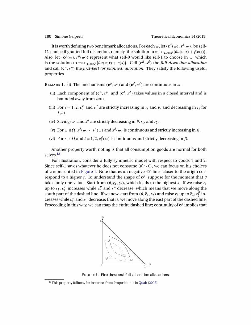
It is worth defining two benchmark allocations. For each ω, let (cd(ω)� sd(ω)) be self-1’s choice if granted full discretion, namely, the solution to max(c�s)∈F {θu(c; r) + βv(s)}.Also, let (cp(ω)� sp(ω)) represent what self-0 would like self-1 to choose in ω, whichis the solution to max(c�s)∈F {θu(c; r) + v(s)}. Call (cd� sd) the full-discretion allocationand call (cp� sp) the first-best (or planned) allocation. They satisfy the following usefulproperties.
Remark 1. (i) The mechanisms (cp� sp) and (cd� sd) are continuous in ω.
(ii) Each component of (cp� sp) and (cd� sd) takes values in a closed interval and isbounded away from zero.
(iii) For i = 1�2, cpi and cdi are strictly increasing in ri and θ, and decreasing in rj forj = i.
(iv) Savings sp and sd are strictly decreasing in θ, r1, and r2.
(v) For ω ∈�, sd(ω) < sp(ω) and sd(ω) is continuous and strictly increasing in β.
(vi) For ω ∈� and i = 1�2, cdi (ω) is continuous and strictly decreasing in β.
Another property worth noting is that all consumption goods are normal for bothselves.13
For illustration, consider a fully symmetric model with respect to goods 1 and 2.Since self-1 saves whatever he does not consume (v′ > 0), we can focus on his choicesof c represented in Figure 1. Note that cs on negative 45° lines closer to the origin cor-respond to a higher s. To understand the shape of cp, suppose for the moment that θtakes only one value. Start from (θ� r1� r2), which leads to the highest s. If we raise r1
up to r1, cp1 increases while cp2 and sp decrease, which means that we move along the
south part of the dashed line. If we now start from (θ� r1� r2) and raise r2 up to r2, cp2 in-creases while c
p1 and sp decrease; that is, we move along the east part of the dashed line.
Proceeding in this way, we can map the entire dashed line; continuity of cp implies that
Figure 1. First-best and full-discretion allocations.
13This property follows, for instance, from Proposition 1 in Quah (2007).
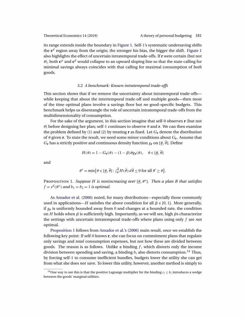
Theoretical Economics 14 (2019) A theory of personal budgeting 181
its range extends inside the boundary in Figure 1. Self-1’s systematic undersaving shiftsthe cd region away from the origin; the stronger his bias, the bigger the shift. Figure 1also highlights the effect of uncertain intratemporal trade-offs. If r were certain (but notθ), both cp and cd would collapse to an upward sloping line so that the state calling forminimal savings always coincides with that calling for maximal consumption of bothgoods.
3.2 A benchmark: Known intratemporal trade-offs
This section shows that if we remove the uncertainty about intratemporal trade-offs—while keeping that about the intertemporal trade-off and multiple goods—then mostof the time optimal plans involve a savings floor but no good-specific budgets. Thisbenchmark helps us disentangle the role of uncertain intratemporal trade-offs from themultidimensionality of consumption.
For the sake of the argument, in this section imagine that self-0 observes r (but notθ) before designing her plan; self-1 continues to observe θ and r. We can then examinethe problem defined by (1) and (2) by treating r as fixed. Let Gr denote the distributionof θ given r. To state the result, we need some minor conditions about Gr. Assume thatGr has a strictly positive and continuous density function gr on [θ�θ]. Define
H(θ)= 1 −Gr(θ)− (1 −β)θgr(θ)� θ ∈ [θ�θ]
and
θ∗ = min{θ ∈ [θ�θ] : ∫θθ′H(θ)dθ ≤ 0 for all θ′ ≥ θ
}�
Proposition 1. Suppose H is nonincreasing over [θ�θ∗]. Then a plan B that satisfiesf = sd(θ∗) and b1 = b2 = 1 is optimal.
As Amador et al. (2006) noted, for many distributions—especially those commonlyused in applications—H satisfies the above condition for all β ∈ [0�1]. More generally,if gr is uniformly bounded away from 0 and changes at a bounded rate, the conditionon H holds when β is sufficiently high. Importantly, as we will see, high βs characterizethe settings with uncertain intratemporal trade-offs where plans using only f are notoptimal.
Proposition 1 follows from Amador et al.’s (2006) main result, once we establish thefollowing key point: If self-0 knows r, she can focus on commitment plans that regulateonly savings and total consumption expenses, but not how these are divided betweengoods. The reason is as follows. Unlike a binding f , which distorts only the incomedivision between spending and saving, a binding bi also distorts consumption.14 Thus,by forcing self-1 to consume inefficient bundles, budgets lower the utility she can getfrom what she does not save. To lower this utility, however, another method is simply to
14One way to see this is that the positive Lagrange multiplier for the binding ci ≤ bi introduces a wedgebetween the goods’ marginal utilities.
182 Simone Galperti Theoretical Economics 14 (2019)
not let self-1 spend all of 1 − s. The literature called this money burning.15 Spending ashare of 1 − s efficiently can achieve any utility obtained by spending 1 − s inefficiently:For all c ∈ R2+, there exists y ≤ c1 + c2 that yields u(c; r) = u∗(y; r), where u∗(y; r) is theindirect utility of spending y. Different realizations of the intratemporal trade-offs mayaffect how self-0 wants to “punish” self-1 for undersaving, holding s fixed. But withoutthat uncertainty, the optimal punishment is unique and can always be achieved withmoney burning, provided that its amount can flexibly depend on the chosen s. Thisrequires more general forms of commitment than budgeting plans. Formally, let
F tc = {(y� s) ∈ R2+ : y + s ≤ 1
}�
Given Dtc ⊂ F tc, self-1 maximizes θu(c; r)+βv(s) subject to c1 + c2 ≤ y and (y� s) ∈Dtc.
Lemma 1. Suppose uncertainty affects only the intertemporal utility trade-off. There ex-ists an optimal D ⊂ F with U(D) = U∗ if and only if there exists an optimal Dtc ⊂ F tc withU(Dtc) = U∗.
Thus, when only the intertemporal trade-off is uncertain, whether consumption in-volves one or multiple goods is irrelevant as long as we allow for general commitmentplans.
Proposition 1 goes one step further by showing that the number of consump-tion goods is irrelevant even when self-1 can use only minimum-savings rules. GivenLemma 1, since the constraint c1 + c2 ≤ y always binds for self-1, the problem becomes
maxDtc⊂F tc
∫ θ
θ
[θu∗(y(θ); r
) + v(s(θ)
)]gr(θ)dθ
s.t.(y(θ)� s(θ)
) ∈ arg max(y�s)∈Dtc
{θu∗(y; r)+βv(s)
}� θ ∈ [θ�θ]�
This is isomorphic to the problem studied by Amador et al. (2006). Proposition 1 thenfollows from their Proposition 3.
3.3 Main results
We now return to the model where both inter- and intratemporal trade-offs are uncer-tain for self-0. The next result is in sharp contrast to the benchmark established before.
Proposition 2. There exists β∗ ∈ (0�1) such that, if β∗ < β < 1. Then every optimalB ∈ B must include binding good-specific budgets.16
The Appendix shows how to derive β∗, which can be significantly smaller than 1.Proposition 2 is silent about whether good-specific budgets are always combined with afloor. Section 3.4 shows that both cases are possible.
Do optimal plans always require good-specific budgets? The answer is no.
15Besides Amador et al. (2006), papers that study money burning in delegation problems include: Am-brus and Egorov (2013, 2017) and Amador and Bagwell (2013, 2016).
16All proofs are provided in the Appendix.

Theoretical Economics 14 (2019) A theory of personal budgeting 183
Proposition 3. There exists β∗ ∈ (0�1) such that if β < β∗, then every optimal B ∈ Binvolves only a binding savings floor.
The Appendix shows how to calculate β∗, which can be significantly larger than 0and depends on G only through its support. Using this, we can show that weaker biasessuffice to render budgets suboptimal when the uncertainty on intratemporal trade-offsshrinks in the following sense.
Corollary 1. Consider two agents who have the same utility functions u and v, andtheir uncertainty has supports [θ�θ]× [r1� r1]× [r2� r2] and [θ�θ]× [r′1� r′1]× [r′2� r′2]. Let β∗and β′∗ be the corresponding thresholds in Proposition 3. If (r ′1� r
′2)� (r1� r2) and (r′1� r
′2)�
(r1� r2), then β′∗ >β∗.
This corollary echoes the benchmark result of Section 3.2: That case corresponds tothe limit as ri − ri → 0 for i = 1�2. We saw that under minor conditions, in the limit,essentially β∗ = 1.
One subtlety of the model is that f , b1, and b2 can bind simultaneously, therebyaffecting self-1’s choices in possibly complex ways. To handle this, the proof proceeds inseveral steps, which are sketched here to also uncover the intuitions for the results.
The first step is to consider how self-0 would use f in isolation. In this case, thebest f lies strictly between the highest and lowest first-best savings, sp and sp, and risesas β falls. Though similar, this step is not a corollary of Amador et al.’s (2006) resultsand uses different techniques. Intuitively, self-0 never finds any s < sp justifiable, and f
never distorts the chosen c because the two selves have the same consumption utility u.Consequently, self-0 always sets f ≥ sp. Setting f = sp cannot be optimal, as raising f abit causes a second-order loss when sp(ω) = sp, but a first-order gain when sp(ω) > sp
and f binds. A similar logic explains why f < sp. Thus, f has to balance the benefit ofcurbing undersaving and the cost of causing oversaving. A lower β raises the optimalf because the benefit of raising f grows if self-1 tends to undersave more, but the coststays the same: When self-0 wants s < f , self-1 does too and f binds for any β. To obtainthese properties, the proof shows that the derivative of self-0’s payoff in f exists, has asimple form, and is decreasing in β. This uses the fact that we can focus on the stateswhere f binds for self-1 and so s = f , which allows us to immediately infer the effectof varying f on self-0’s savings utility, v. Since both selves share u, the effect on self-0’sconsumption utility can be inferred from self-1’s indirect utility from spending 1 − f viaLagrangian sensitivity analysis, which links this effect to the marginal utility of any goodat the chosen c. These effects are shown to matter for a set of states with strictly positiveprobability using the continuity of self-1’s choices in f and ω and the full support of G.
The second step is to consider how self-0 would use bi in isolation. It turns out thatcapping even only one good dominates granting self-1 full discretion. To see why, startfrom the level of bi where it starts to bind (i.e., bi = cdi = maxω cdi (ω)). Lowering bi createsa benefit and a cost for self-0 when bi binds. The cost is that it distorts consumption, butthis is initially a second-order cost, because the full discretion cd is efficient in the senseof equalizing marginal utilities between goods. The benefit is that bi curbs undersaving,

184 Simone Galperti Theoretical Economics 14 (2019)
which is of first-order importance for self-0. Overall bi should then benefit self-0, butthere is a subtlety: Self-1 should not reallocate income to the unrestricted cj much fasterthan to s, which is not obvious and need not be true. This key property holds for theadditively separable u, but also more generally (see Section 4). Once this is established,the proof uses the fact that both selves share u to show that self-0’s payoff can be writtenas her savings utility scaled by (1 −β) plus self-1’s total payoff subject to bi. Lagrangiansensitivity analysis on the latter pins down the second-order negative effects of bi. Theformer part directly quantifies the first-order positive effects of bi. These effects againmatter for a set of states with strictly positive probability for the same reasons as before.
These points highlight the general mechanism whereby multidimensional con-sumption can help to curb the consequences of present bias. A budget bi incentivizesself-1 to save more because it forces him to choose inefficient bundles—not just to spendless on ci, which he could fully shift to cj—and this inefficiency limits the present utilityself-1 can gain by undersaving.
The above two steps are combined to obtain Proposition 2. Intuitively, when presentbias is weak, an optimal plan must use budgets because they help improve savings whendoing so via f would require it to be too tight. Consider Figure 2, which focusses on con-sumption choices and reports the full-discretion and first-best allocations from Figure 1.Graphically, b1 defines a vertical line allowing only c1s to its left, b2 defines a horizontalline allowing only c2s below it, and f defines a line with slope −1 allowing only cs belowit. Thus, in Figure 2(b) for instance, self-1 must choose c within the diamond-shaped re-gion to the southwest of the solid lines f , b1, and b2. Uncertain intratemporal trade-offsimply that the states where both selves want to spend the most on c1 or c2 (which map tothe light-shaded areas) are not the states where they want to save the least (which mapto the dark-shaded areas). Indeed, by Remark 1, for i = 1�2 and k= p�d,
cki = cki (θ� ri� r−i) > cki (θ� ri� r−i) and sk = sk(θ� ri� r−i) < sk(θ� ri� r−i)�
We saw that if self-0 can use only f , she relaxes it as β rises; that is, the f line moves far-ther away from the origin. Consequently, f constrains choices in the dark-shaded area,but at some point stops affecting them in the light-shaded areas: compare panel (a)
Figure 2. Optimal budgeting plans: Intuition.
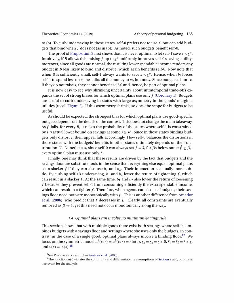
Theoretical Economics 14 (2019) A theory of personal budgeting 185
to (b). To curb undersaving in these states, self-0 prefers not to use f , but can add bud-gets that bind when f does not (as in (b)). As noted, such budgets benefit self-0.
The proof of Proposition 3 first shows that it is never optimal to let self-1 save s < sp.Intuitively, if B allows this, raising f up to sp uniformly improves self-0’s savings utility;moreover, since all goods are normal, the resulting lower spendable income renders anybudget in B less likely to bind and distort c, which again benefits self-0. Now note thatwhen β is sufficiently small, self-1 always wants to save s < sp. Hence, when bi forcesself-1 to spend less on ci, he shifts all the money to cj , but not s. Since budgets distort c,if they do not raise s, they cannot benefit self-0 and, hence, be part of optimal plans.
It is now easy to see why shrinking uncertainty about intratemporal trade-offs ex-pands the set of strong biases for which optimal plans use only f (Corollary 1). Budgetsare useful to curb undersaving in states with large asymmetry in the goods’ marginalutilities (recall Figure 2). If this asymmetry shrinks, so does the scope for budgets to beuseful.
As should be expected, the strongest bias for which optimal plans use good-specificbudgets depends on the details of the context. This does not change the main takeaway.As β falls, for every B, it raises the probability of the states where self-1 is constrainedby B’s actual lower bound on savings at some s ≥ sp. Since in these states binding bud-gets only distort c, their appeal falls accordingly. How self-0 balances the distortions inthose states with the budgets’ benefits in other states ultimately depends on their dis-tribution G. Nonetheless, since self-0 can always set f = s, for βs below some β ≥ β∗,every optimal plan must use only f .
Finally, one may think that these results are driven by the fact that budgets and thesavings floor are substitute tools in the sense that, everything else equal, optimal plansset a slacker f if they can also use b1 and b2. Their interaction is actually more sub-tle. By curbing self-1’s undersaving, b1 and b2 lower the return of tightening f , whichcan result in a slacker f . At the same time, b1 and b2 also lower the return of looseningf because they prevent self-1 from consuming efficiently the extra spendable income,which can result in a tighter f . Therefore, when agents can also use budgets, their sav-ings floor need not vary monotonically with β. This is another difference from Amadoret al. (2006), who predict that f decreases in β. Clearly, all constraints are eventuallyremoved as β → 1, yet this need not occur monotonically along the way.
3.4 Optimal plans can involve no minimum-savings rule
This section shows that with multiple goods there exist both settings where self-0 com-bines budgets with a savings floor and settings where she uses only the budgets. In con-trast, in the case of a single good, optimal plans always involve a binding floor.17 Wefocus on the symmetric model u1(c; r) = u2(c; r) = r ln(c), r1 = r2 = r > 0, r1 = r2 = r > r,and v(s)= ln(s).18
17See Propositions 2 and 10 in Amador et al. (2006).18The function ln(·) violates the continuity and differentiability assumptions of Section 2 at 0, but this is
irrelevant for the analysis.

186 Simone Galperti Theoretical Economics 14 (2019)
Proposition 4. There exist full-support distributions G such that f , b1, and b2 are allbinding for every optimal B ∈ B. There also exist full-support distributions G′ such that,for every optimal B ∈ B, b1 and b2 are binding, but f never binds.
While the result holds for full-support distributions, its intuition can be best ex-plained by considering a three-state case. Let ω0 = (θ� r1� r2), ω1 = (θ� r1� r2), andω2 = (θ� r1� r2) with respective probabilities g, 1
2(1 − g), and 12(1 − g). Remark 1 and
symmetry imply that
sd(ω0)< sd
(ω1) = sd
(ω2)� cd1
(ω2) = cd2
(ω1)< cd1
(ω1) = cd2
(ω2)� cd1
(ω0) = cd2
(ω0);
similar properties hold for (cp� sp). By continuity, there exists β < 1 sufficiently highthat sd(ω1) = sd(ω2) > sp(ω0); hereafter, fix such a β. There exists θ sufficiently closeto θ that c
p1 (ω
1) > cp1 (ω
0) and cp2 (ω
2) > cp2 (ω
0). Figure 3(a) represents this situation,focussing again on consumption. Concretely, imagine that Ann has two friends, Beckyand Cindy. In a given week, Ann may go out with Becky (ω1), Cindy (ω2), or both together(ω0). Ann likes shopping for clothes with Becky and trying new restaurants with Cindy.When out with both, she enjoys both activities even more. Finally, Ann anticipates thatonce in the store or the restaurant, she will tend to spend too much.
One can show that if Ann deems going out with both friends sufficiently likely (i.e.,g > g∗ for some g∗ ∈ (0�1)), then she wants to set a binding f as well as budgets for bothgoods. In fact, the optimal B satisfies f = sp(ω0), b1 = c
p1 (ω
1), and b2 = cp2 (ω
2).19 Theintuition is this. If Ann was sure to go out with one friend at a time, she could set f so asto eliminate splurging in ω1 and ω2: this f corresponds to the dotted line in Figure 3(a).However, this f will be too stringent if she ends up going out with both friends. Sincethis is very likely, Ann prefers f = sp(ω0). She knows that this f will not bind when sheis out with only one friend. But for this case she can curb overspending using b1 and b2;also, here she can do so without affecting her choice in ω0.
Figure 3. Three-state example (cdi = cd(ωi) and cpi = cp(ωi)).
19This claim is shown as part of the constructive proof of Proposition 4. The specific levels of b1 and b2are just a by-product of logarithmic payoffs.

Theoretical Economics 14 (2019) A theory of personal budgeting 187
A simple change of this three-state setting suffices to explain why optimal plans caninvolve only good-specific budgets. Fix g > g∗ and all the other parameters except θ.If we increase θ, both selves want to consume more in ω0. This eventually leads to asituation as in Figure 3(b), where c
p1 (ω
0) > cp1 (ω
1) and cp2 (ω
0) > cp2 (ω
2). In this case,Ann wants to keep b1 and b2, but drop f . In fact, her optimal B satisfies b1 = b2 andcpi (ω
i) < bi < cpi (ω
0) for every i = 1�2, but f = 0.20 Figure 3(b) helps with the intuition.
Now Ann is willing to spend even more in ω0. Therefore, the budgets she would set tocurb splurging in ω1 and ω2 start to bind also in ω0. As a result, she wants to relax them.She realizes, however, that her first-best spending on clothes and food in ω0 is just abovethose budgets. Relaxing them a bit will allow her to curb splurging in ω1 and ω2 as wellas ω0. Since these budgets already push savings above the first best in ω0, Ann cannotbenefit by adding a binding f .
In short, a weakly present-biased agent may use only good-specific budgets for thefollowing reason. To curb undersaving in states with large asymmetry in consumptionmarginal utilities, she may prefer to use the budgets rather than a savings floor, whichwould have to be too stringent. Together the budgets then impose a cap on total spend-ing. If this already ensures sufficiently high savings in states where present consumptionis very valuable overall, then any binding floor will have to cause additional oversavingand this inefficiency can exceed the floor’s commitment benefits.
4. Discussion
Theory and evidence
How does this theory relate to the evidence on budgeting and other explanationsthereof? One finding is that people may set budgets on “unobjectionable goods likesports tickets and blue jeans” (Heath and Soll 1996) or housing, food, and even charita-ble giving (Thaler 1985, 1999). This is difficult to explain with an alternative theory ar-guing that people set budgets for the goods they find tempting (“vice goods”), althoughthis can be true in some cases. By contrast, present bias combined with uncertain in-tratemporal trade-offs can lead people to set budgets on “unobjectionable goods,” asdoing so helps them manage their overall tendency to overspend better than with just asavings floor. Thus, it is not the tempting nature of a good that matters.
Another plausible theory is that budgeting is a technique to simplify the complexmatter of household finance (Simon 1997, Johnson 1984). This theory is complementaryto the one in this paper, but again struggles to explain some evidence. For instance,it is not clear why computational complexity would lead people to systematically setbudgets that seem too strict and to cause underconsumption, as found by Heath and Soll(1996). By contrast, present-biased people do optimally set budgets that systematicallybind and thus exhibit those properties.
20Again, this claim is shown as part of the constructive proof of Proposition 4. Note that, although thisthree-state example is intuitive, it takes some work to rule out the possibility of multiple, perhaps asym-metric, optimal plans featuring different properties from those in the proposition.

188 Simone Galperti Theoretical Economics 14 (2019)
The prediction that only weakly biased agents should use good-specific budgets isconsistent with some findings in Antonides et al. (2011). In their sample, people who ex-hibit a “short-term time orientation” (which according to their description is consistentwith strong present bias) are less likely to use budgets than people who exhibit a “long-term time orientation” (a weak bias). Unfortunately, Antonides et al. (2011) do not mea-sure how stringent budgets or floors are in relation to present bias. For that matter, wesaw that this relation need not be monotonic. As an alternative explanation, strongly bi-ased agents may not use budgets because they are less sophisticated or able to commit.The anticipated bias (not the true one) is what matters for self-0’s problem, however.Therefore, by Proposition 2 underestimating that bias—not entirely, of course—may ac-tually render it more likely that self-0 finds budgets beneficial. If this same agent wereinstead sophisticated, he might not adopt any budget by Proposition 3. We also saw thatonce a strongly biased agent can use a savings floor, the reason why budgets do not workfor him is not that he cannot honor them: Even if he could, they would strictly lower hisutility.
Relaxing separability
The message of the paper generalizes to settings where utility is not separable acrossgoods. Continue to assume that u(c; r) is strictly concave in c and twice differentiablewith continuous uci(c; r) > 0 and ucicj (c; r) in both arguments for all i and j. We sawthat budgets help curb self-1’s undersaving if (a) they increase savings and (b) there ex-ist states that call for high consumption of some good, but not of all goods. Property (b)holds if some good is a sufficiently strong substitute of all other goods. Property (a) holdsif the capped good is a Hicks substitute of savings (Howard 1977); in general, such a goodalways exists (Madden 1991, Theorem 2). As noted, however, a budget has to curb un-dersaving faster than it exacerbates overspending on other goods for it to benefit self-0.Given space constraints, these properties are stated directly in terms of allocations.
Condition 1. Both (cp� sp) and (cd� sd) are interior for every ω. Both sp and sd arestrictly decreasing in θ and ri for i = 1�2. There exists some good j that satisfies thefollowing statements: (i) cpj and cdj are strictly increasing in θ and rj , and decreasing in
ri for i = j; (ii) there exists ε > 0 such that, for every bj < maxω cdj (ω), self-1’s optimal
(c∗� s∗) subject to plans involving only bj satisfies s∗(ω) − sd(ω) ≥ ε[cdj (ω) − c∗j (ω)] for
all ω ∈ �.
Appendix A.6 presents an example that satisfies Condition 1.To state the result, consider a more general class of budgeting plans, denoted by B,
which allow us to also set good-specific floors and a savings cap,
B = {(c� s) ∈ F : f0 ≤ s ≤ b0� f1 ≤ c1 ≤ b1� f2 ≤ c2 ≤ b2
}�
where fi� bi ∈ [0�1] satisfy fi ≤ bi for i = 0�1�2 and f0 + f1 + f2 ≤ 1.
Proposition 5. Under Condition 1, there exists β∗ ∈ (0�1) such that, if β∗ <β< 1. Thenevery optimal B ∈ B must use distorting good-specific restrictions.

Theoretical Economics 14 (2019) A theory of personal budgeting 189
The proof is omitted, because using Condition 1, one can adapt the proof of Propo-sition 2 to show that plans using only f0 are strictly dominated for sufficiently high β.Since setting a binding b0 is never optimal, the result follows.
Do optimal good-specific restrictions always take the form of budgets? The answerdepends on the substitutability and complementarity between goods and between eachgood and savings, which can be affected by the restrictions themselves. A sufficient con-dition for optimal plans to never use f1 and f2 is that all goods are Hicks substitutes andcollectively sufficiently normal (see Ellis and Naughton 1990 for a formal statement ofthis property). Given this, by Theorems 3 and 4 of Madden (1991) two goods remainsubstitutes independently of which goods are restricted, and Ellis and Naughton’s (1990)analysis implies that, given any f1 and f2, relaxing them raises s. Hence, since f1 and f2
distort consumption, they strictly harm self-0. Optimal plans use only b1 and b2 for theexample in Appendix A.6.
General mechanisms
One may wonder what the best among all conceivable plans (not just those in B) lookslike and whether it belongs to B. These are important questions, but also hard inthe presence of multidimensional consumption and uncertainty. The main challengescome from the income constraint and the complexity of the incentive constraints, whichas usual cannot be reduced to only the local ones. Here one can try to apply the insightsfrom multidimensional screening (Rochet and Stole 2003), but substantive differencesremain. First, screening problems allow for transfers. Here one can view the utility fromsavings as a transfer and use Rochet and Choné’s (1998) approach to simplify the incen-tive constraints and self-0’s objective. But the state-wise income constraint (the seconddifference from screening) cannot be simplified. General techniques exist for handlingsuch constraints (Luenberger 1969), but unlike in the case of unidimensional consump-tion, here they do not go far.
5. Concluding remarks
This paper provides a theoretical analysis of the link between self-control problems andpersonal budgeting using a parsimonious consumption–savings model with a present-biased agent. Unlike minimum-savings rules, good-specific spending caps help tocurtail overspending because they cause inefficiencies in consumption that lower thereturn from undersaving, thereby counteracting present bias. Consequently, good-specific budgets are no free lunch and are used only by agents who are weakly biased anduncertain about their intratemporal trade-offs between goods. Those who are stronglybiased or do not face such uncertainty prefer to rely exclusively on a minimum-savingsrule.
This theory offers insights into the subtle forces underlying a widely observed phe-nomenon, which has far-reaching consequences for consumer behavior and welfare byaffecting demand differently from satiation and income effects, and by significantly con-tributing to households’ wealth accumulation. The theory matches existing empirical
190 Simone Galperti Theoretical Economics 14 (2019)
findings, such as that people often set budgets for goods normally not viewed as tempt-ing and only those who exhibit weak present bias seem to use budgets. The theory alsosuggests new directions for enriching the sparse evidence on budgeting by demonstrat-ing its dependence on uncertain intratemporal trade-offs, and for designing commit-ment devices whose functions are targeted to the right type of present-biased agents.
Appendix
A.1 Technical lemmas
Lemma 2. There exists B that maximizes U(B) over B.
Proof. Each B ∈ B can be viewed as an element (f�b) of the compact set [0�1]n+1. Thus,we can think that self-0 chooses (f�b) ∈ [0�1]n+1.
Given any such (f�b), let (c(ω|f�b)� s(ω|f�b)) be self-1’s optimal allocation in stateω from the compact set Bf�b defined by (f�b). Since Bf�b is convex (Theorem 2.1 inRockafellar 1997), (c(ω|f�b)� s(ω|f�b)) is unique for every ω ∈ � by strict concavity ofself-1’s utility function. Clearly, the correspondence that for each (f�b) ∈ [0�1]n+1 mapsto Bf�b is nonempty, compact valued, and continuous. It follows from the maximumtheorem that (c(ω|·� ·)� s(ω|·� ·)) is continuous for every ω ∈�.
We can now show that self-0’s payoff is continuous in (f�b). For each (f�b) ∈[0�1]n+1, let
U(f�b) =∫�
[θu
(c(ω|f�b); r
) + v(s(ω|f�b)]dG(ω)�
Since the integrand is continuous in (f�b) for every ω ∈ � and is uniformly boundedover B(f�b), Lebesgue’s dominated convergence theorem implies the claimed propertyof U(·� ·).
A second application of the maximum theorem gives the result.
Lemma 3. Fix i ∈ {1� � � � � n} and consider B ∈ B with bj = 1 for all j = i. For any ω, ifbi < cdi (ω), self-1 chooses s > sd(ω) and cj > cdj (ω) for all j = i.
Proof. Let i = 1 and b1 ∈ (0� cd1 (ω)). Consider self-1’s problem in state ω to maximizeθu(c� r) + βv(s) for (c� s) ∈ F subject to c1 ≤ b1. The first-order conditions of its La-grangian are βv′(s(ω)) = μ(ω), θu1
c(c1(ω); r1)= μ(ω)+λ1(ω), and θuic(ci(ω); ri) = μ(ω)
for all i = 1, where μ(ω) ≥ 0 and λ1(ω) ≥ 0 are the Lagrange multipliers for∑n
i=1 ci ≤ 1and c1 ≤ b1.
Suppose s(ω) ≤ sd(ω). Since c1(ω) = b1 < cd1 (ω) and s(ω) + ∑j cj(ω) = sd(ω) +∑
j cdj (ω) = 1 by strong monotonicity of preferences, cj(ω) > cdj (ω) for some j = 0�1.
By strict concavity of uj and v, θujc(cj(ω); rj) < θujc(c
dj (ω); rj) = βv′(sd(ω)) ≤ βv′(s(ω)).
This violates the first-order conditions for c(ω). So we must have s(ω) > sd(ω). Thisin turn implies that θujc(cj(ω); rj) = βv′(s(ω)) < βv′(sd(ω)) = θu
jc(c
dj (ω); rj) for j = i. By
concavity, cj(ω) > cdj (ω) for j = 1.

Theoretical Economics 14 (2019) A theory of personal budgeting 191
For k= p�d, let sk = minω sk(ω) and sk(ω) = maxω sk(ω). Focussing on f ∈ [sd� sp],21
denote by Bf the corresponding policy in B.
Lemma 4. Define �(f) = {ω ∈ � : sd(ω) ≤ f } and let cf (ω) be the maximizer of u(c; r)subject to
∑ni=1 ci ≤ 1 − f . Then U(Bf ) is differentiable in f over [sd� sp] with
d
dfU(Bf ) =
∫�(f)
[v′(f )− θuci
(cf (ω); r
)]dG for any i = 1� � � � � n�
Proof. Given f and any ω, define
u(f ;ω) ≡ u(cf (ω); r
) = max{c∈Rn+:∑n
i=1 ci≤1−f }u(c; r)
and U(f ;ω) = θu(f ;ω) + v(f ). Since u(·; r) is strictly concave in c, so is u(·; r) in f bystandard arguments. Hence, U(·;ω) is also strictly concave in f . Now consider U ′(f ;ω).Whenever it is defined, U ′(f ;ω) = θu′(f ;ω)+ v′(f ). By first-order conditions of the La-grangian defining u(f ; r), we have uci(cf (ω); r) = λ(ω; f ) for i = 1� � � � � n, where λ(ω; f )is the Lagrange multiplier for
∑ni=1 ci ≤ 1 − f . Since cf (ω) is continuous in f for ev-
ery ω, so is λ(ω; f ). By Theorem 1 of Luenberger 1969, p. 222) λ(ω; f ′)(f ′′ − f ′) ≤u(f ′; r) − u(f ′′; r) ≤ λ(ω; f ′′)(f ′′ − f ′) for every f ′� f ′′ ∈ (0�1). Continuity of λ(ω; ·) im-plies that u′(f ; r) exists for every f ∈ (0�1) and u′(f ; r) = −λ(ω; f ) = −uci(cf (ω); r).Therefore,
U ′(f ;ω) = v′(f )− θuci(cf (ω); r
)� ω ∈�� (3)
For any f , denote by (cf � sf ) self-1’s behavior as a function of ω under Bf . By themaximum theorem, (cf (ω)� sf (ω)) is continuous in both f and ω. Since, fixing any s,both selves would choose the same c in every ω, by definition
�(f) ≡ U(Bf )=∫�U
(sf (ω);ω)
dG�
Consider any f > f and recall that �(f)= {ω : sd(ω) ≤ f }. Then
�(f)−�(f ) =∫�(f)
[U(f ;ω)− U
(sf (ω);ω)]
dG
=∫�(f)∩(�(f ))c
[U(f ;ω)− U
(sf (ω);ω)]
dG+∫�(f )
[U(f ;ω)− U(f ;ω)
]dG;
the first equality holds because sf (ω) = sf (ω) for ω /∈ �(f) and sf (ω) = f for ω ∈ �(f).Divide both sides by f − f and consider the limit as f ↓ f . First, for all ω, we have
limf↓f
U(f ;ω)− U(f ;ω)
f − f= U ′(f ;ω)�
21Any other f is dominated by one in this range.
192 Simone Galperti Theoretical Economics 14 (2019)
Since U(·;ω) is concave,∣∣∣∣ U(f ;ω)− U(f ;ω)
f − f
∣∣∣∣ ≤ max{∣∣U ′(f ;ω)
∣∣� ∣∣U ′(f ;ω)∣∣}�
Since U ′(f ;ω) is continuous in ω and f as illustrated by (3), |U ′(f ;ω)| is bounded bysome M < +∞ for (f�ω) ∈ [sd� sp] × �. Therefore, by Lebesgue’s bounded convergencetheorem,
limf↓f
∫�(f )
U(f ;ω)− U(f ;ω)
f − fdG=
∫�(f )
U ′(f ;ω)dG�
Consider now the second part of the limit. Again, by concavity of U(·;ω) and sincesf (ω) ∈ [sd� sp] for f ∈ [sd� sp], we have
∣∣∣∣ U(f ;ω)− U(sf (ω);ω)
f − sf (ω)
∣∣∣∣ ≤M�
Therefore,
∣∣∣∣∫�(f)∩(�(f ))c
U(f ;ω)− U(sf (ω);ω)
f − fdG
∣∣∣∣ ≤∫�(f)∩(�(f ))c
∣∣∣∣ U(f ;ω)− U(sf (ω);ω)
f − f
∣∣∣∣dG≤
∫�(f)∩(�(f ))c
∣∣∣∣ U(f ;ω)− U(sf (ω);ω)
f − sf (ω)
∣∣∣∣dG≤ M
∫�(f)∩(�(f ))c
dG�
Observe that �(f) ∩ (�(f ))c = {ω : f < sf (ω) ≤ f }, which converges to an empty setas f ↓ f . Since then the second part of the limit converges to zero as f ↓ f , for everyf ∈ [sd� sp),
�′(f+) =∫�(f )
U ′(f ;ω)dG�
A similar argument implies that �′(f−) = ∫�(f )
U ′(f ;ω)dG for every f ∈ (sd� sp]. Hence,
�(f) is differentiable over [sd� sp].
A.2 Proof of Lemma 1
Fix r. Recall the definition of U(D) in (1) of the main text and that (c(θ)� s(θ)) representsself-1’s optimal choice in state θ. There exists D ⊂ F such that U(D) ≥ U(D′) for all D′ ⊂F if and only if there exist functions χ : [θ�θ] → Rn+ and t : [θ�θ] → R+ that satisfy thefollowing two conditions:
Condition 1. For all θ�θ′ ∈ [θ�θ],θu
(χ(θ); r
) +βv(t(θ)
) ≥ θu(χ(θ′); r
) +βv(t(θ′))
Theoretical Economics 14 (2019) A theory of personal budgeting 193
andn∑
i=1
χi(θ)+ t(θ)≤ 1�
Condition 2. The pair (χ� t) maximizes
∫ θ
θ
[θu
(χ(θ); r
) + v(t(θ)
)]gr(θ)dθ�
By contrast, there exists Dtc ⊂ F tc such that U(Dtc) ≥ U(Dtc) for all Dtc ⊂ F tc if andonly if there exist functions ϕ : [θ�θ] → R+ and τ : [θ�θ] → R+ that satisfy the followingtwo conditions:
Condition 1′ . For all θ�θ′ ∈ [θ�θ],θu∗(ϕ(θ); r
) +βv(τ(θ)
) ≥ θu∗(ϕ(θ′); r
) +βv(τ(θ′))�
where u∗(y; r) = max{c′∈Rn+:∑ni=1 c
′i≤y} u(c′; r) and
ϕ(θ)+ τ(θ)≤ 1�
Condition 2′ . The pair (ϕ�τ) maximizes
∫ θ
θ
[θu∗(ϕ(θ); r
) + v(τ(θ)
)]gr(θ)dθ�
Suppose (χ� t) that satisfies Conditions 1 and 2. Then, by our discussion on moneyburning before the statement of Lemma 1, there exists a function ϕ : [θ�θ] → R+ suchthat u∗(ϕ(θ); r) = u(χ(θ); r) and ϕ(θ) ≤ ∑n
i=1 χi(θ) for all θ ∈ [θ�θ]. Hence, letting τ ≡ t,we have that (ϕ�τ) satisfies both Conditions 1′ and 2′.
Suppose (ϕ�τ) satisfy Conditions 1′ and 2′. For every θ ∈ [θ�θ], let
χ(θ) = arg max{c∈Rn+:∑n
i=1 ci≤ϕ(θ)}u(c; r)�
Then, by definition, u(χ(θ); r) = u∗(ϕ(θ); r) for all θ ∈ [θ�θ]. Letting t ≡ τ, we have that(χ� t) satisfies both Conditions 1 and 2.
A.3 Proof of Proposition 2
The proof uses the following three lemmas.
Lemma 5. When self-0 can set only f , every optimal f satisfies sp < f < sp.
Proof. We will show that �′(f ) > 0 for all f ∈ (sd� sp] and �′(f−) < 0 for f = sp. Recallthat (cf � sf ) is continuous in f for every ω and, therefore, so is �(f). These observationsimply that every optimal f ∗ is in (sp� sp).
194 Simone Galperti Theoretical Economics 14 (2019)
For any f ∈ (sd� sp], define �+(f ) = {ω : sp(ω) > f } and �−(f ) = {ω : sp(ω) ≤ f }. Forω ∈ �+(f ), consider the fictitious problem maximizing θu(c; r) + v(s) for (c� s) ∈ Rn+1+subject to s + ∑
i ci ≤ 1 and s ≤ f . Letting μ(ω) and φ+(ω) be the corresponding La-grange multipliers, the first-order conditions are22 v′(s) = μ(ω)+φ+(ω) and θuci(c; r) =μ(ω) for all i. Clearly, s = f and φ+(ω) > 0 for ω ∈ �+(f ). Also, conditional on s = f ,both selves would choose the same c in state ω, which is, therefore, cf (ω). Using (3), itfollows that, for every i,
φ+(ω) = v′(f )− θuci(cf (ω);ω) = U ′(f ;ω)� ω ∈�+(f )� (4)
For ω ∈ �−(f ), consider the fictitious problem of maximizing θu(c; r) + v(s) for (c� s) ∈Rn+1+ subject to s+∑
i ci ≤ 1 and s ≥ f . Letting μ(ω) and φ−(ω) be the corresponding La-grange multipliers, the first-order conditions are v′(s) = μ(ω) − φ−(ω) and θuci(c; r) =μ(ω) for all i. Clearly, s = f and φ−(ω) ≥ 0 for ω ∈ �−(f ). Also, conditional on s = f ,both selves would choose the same c in state ω, which is, therefore, cf (ω). Using (3), itfollows that, for every i,
φ−(ω) = θuci(cf (ω); r
) − v′(f ) = −U ′(f ;ω)� ω ∈�−(f )�
Consider any f ∈ (sd� sp]. Recall that �(f) = {ω : sd(ω) ≤ f }. Using Lemma 4, wehave
�′(f ) =∫�(f)∩�+(f )
U ′(f ;ω)dG+∫�(f)∩�−(f )
U ′(f ;ω)dG =∫�(f)∩�+(f )
φ+(ω)dG�
where the last equality follows because either �−(f ) = ∅ or φ−(ω) = 0 for ω ∈ �−(f ).The function φ+(ω) is strictly positive over �(f) ∩ �+(f ). We need to show thatG(�(f) ∩ �+(f )) > 0, which implies �′(f ) > 0. This is immediate if f ∈ (sd� sp), be-cause �+(f ) = �. Consider f = sp. Clearly, �(sp) ∩ �+(sp) contains the open set�
◦(sp) ∩ �+(sp) = {ω : sd(ω) < sp < sp(ω)}. If this set is nonempty, we are done
because G has full support. Both �◦(sp) and �+(sp) are nonempty. Suppose that
�+(sp)∩�◦(sp) = ∅. Then, for every ω ∈ �+(sp), we have sd(ω) ≥ sp and that �
◦(sp) ⊂
�−(sp) = {ω : sp(ω) = sp}. Now, consider ω ∈ �◦(sp) and any sequence {ωn} in �+(sp)
converging to ω. We have that limωn→ω inf sd(ωn) ≥ sp > sd(ω). But this violates thecontinuity of sd—a contradiction.
Now consider f = sp. Again using Lemma 4, we have
�′(sp−) =∫�(sp)
U ′(sp;ω)dG =
∫�U ′(sp;ω)
dG= −∫�φ−(ω)dG�
where φ−(ω) > 0 for all ω such that sp(ω) < sp. Therefore, �′(sp−) < 0.23
22Here—and in the other proofs—the complementary slackness conditions are omitted for simplicity.23It is easy to see that the optimal f satisfies f ≤ sp. Suppose f ∈ (sp�1). Then, for all ω, self-1 chooses
s(ω) = f and c(ω) = cf (ω). Take any f ′ ∈ (sp� f ). Then, for every ω, f ′ = ζ(ω)f + (1 − ζ(ω))sp(ω) forsome ζ(ω) ∈ (0�1). Therefore, for every ω, U(f ′;ω) > U(f ;ω) because U(sp(ω);ω) > U(f ;ω) and U(·;ω)
is strictly concave. It follows that self-0’s payoff is strictly larger under f ′ than under f .
Theoretical Economics 14 (2019) A theory of personal budgeting 195
Let E(β) be the set of optimal floors and let u∗(y; r) be the indirect utility of spendingy ∈ [0�1].
Lemma 6. The set E(β) is decreasing in β in the strong set order.24 The largest optimalf converges monotonically to sp as β ↑ 1. There exists β > 0 such that E(β) = {f } for all
β ≤ β, where f satisfies f < sp and
U(Bf ) = maxf∈[sp�sp]
∫�
[θu∗(1 − f ; r)+ v(f )
]dG�
Proof. Fix f ∈ [sd� sp]. The set �(f) in Lemma 4 depends on β via (cd� sd). By standardarguments, if β < β′ < 1, then sd(ω;β) < sd(ω;β′) for every ω and, hence, �(f ;β′) ⊂�(f ;β). Also, �−(f ) ⊂�(f ;β) for every β< 1 because sd(ω;β) < sp(ω) for every ω. So,if β<β′ < 1,
�′(f ;β)−�′(f ;β′) =∫(�(f ;β)\�(f ;β′))∩�+(f )
φ+(ω)dG ≥ 0�
where the inequality uses (4). By standard results, E(β) decreases in the strong set order.Define f (β) = max{f : f ∈ E(β)}. Since f (β) ≥ sp for all β and f (·) is decreas-
ing, limβ↑1 f (β) exists; denote it by f (1−) ≥ sp. Clearly, f (1) = sp. Now suppose thatf (1−) > f(1). By a similar argument, for any f > sp, limβ↑1 �
′(f ;β) exists and equals− ∫
�−(f ) φ(ω)dG < 0. Therefore, for β close enough to 1, f (β) ≥ f (1−) cannot be
optimal—a contradiction that implies f (1−) = f (1).Note that sd(β) = max� sd(s;β) falls monotonically to 0 as β ↓ 0. Let β = max{β ∈
[0�1] : sd(β) ≤ sp}, which is strictly positive because sp > 0. Then �(f) = � for all β ≤ β
and f ∈ [sp� sp], and, hence,
�(f ;β) =∫�
[θu
(cf (ω); r
) + v(f )]dG� (5)
From the proof of Lemma 4, u(cf (ω); r) = u(f ;ω) is strictly concave in f for all ω. Thus,the maximizer of (5) is unique. From the proof of Lemma 5, the derivative of (5) is nega-tive at sp and, hence, f < sp.
We now show that self-0 benefits from using only bi.
Lemma 7. Fix i and consider plans Bbi with bj = 1 for all j = i and f = 0. There existsbi < maxω cdi (ω) ≡ cdi such that U(Bbi) > U(F).
Proof. Fix i = 1 and any b1 ∈ (0� cd1 ]. Let (cb1� sb1) describe self-1’s choices under Bb1
and let
�(b1)=∫�
[θu
(cb1(ω); r
) + v(sb1(ω)
)]dG�
24Given two sets E and E′ in R, E ≥E′ in the strong set order if, for every f ∈E and f ′ ∈ E′, min{f� f ′} ∈ E′and max{f� f ′} ∈ E (Milgrom and Shannon 1994).
196 Simone Galperti Theoretical Economics 14 (2019)
Let �(b1) = {ω : cd1 (ω) > b1}. Since cd1 is continuous, �(b1) is nonempty and open ifb1 < cd1 , and, hence, G(�(b1)) > 0. We have
�(b1)−�(cd1
) =∫�(b1)
{[θu
(cb1(ω); r
) + v(sb1(ω)
)] − [θu
(cd(ω); r
) + v(sd(ω)
)]}dG
= (1 −β)
∫�(b1)
[v(sb1(ω)
) − v(sd(ω)
)]dG
+∫�(b1)
[V
(cb11 (ω);ω) − V
(cd1 (ω);ω)]
dG�
where
V (b1;ω) = max{(c�s)∈Rn+1+ :∑n
j=1 cj≤1�c1≤b1}
{θu(c; r)+βv(s)
}�
Clearly, V (cd1 (ω);ω) ≥ V (b1;ω) for all ω. From the first-order conditions of the La-
grangian defining V (b1;ω), we have λ1(ω; b1) = θu1c(c
b11 (ω); r1) − βv′(sb1(ω)), where
λ1(ω; b1) is the Lagrange multiplier for c1 ≤ b1. Since (cb1(ω)� sb1(ω)) is continuous inb1 and ω, so is λ1(ω; b1). Again by Theorem 1 of Luenberger 1969, p. 222), V ′(b1;ω)
exists for all b1 and equals λ1(ω; b1). It follows that V ′(cd1 (ω);ω) = 0 for all ω by the
definition of (cd� sd). By the mean value theorem (MVT), V (cb11 (ω);ω) − V (cd1 (ω);ω) =
V ′(χ(ω);ω)(cb11 (ω)− cd1 (ω)) and v(sb1(ω))−v(sd(ω)) = v′(ξ(ω))(sb1(ω)− sd(ω)), where
χ(ω) ∈ [cb11 (ω)� cd1 (ω)] and ξ(ω) ∈ [sd(ω)� sb1(ω)].
Let bε1 = cd1 − ε for some ε > 0. Fix ω ∈ �(bε1) and, for now, drop the dependence
on ω. Recall that sbε1 + ∑
i cbε1i = sd + ∑
i cdi = 1. Since sb
ε1 > sd for ε > 0 (Lemma 3), we
can write
−cbε11 − cd1
sbε1 − sd
= 1 +∑j =1
cbε1j − cdj
sbε1 − sd
� (6)
Now, for any bε1 , the first-order condition βv′(s) − θujc(cj; rj) = 0 must hold for every
j = 1. Therefore, again by the MVT, for all j = 1,
cbε1j − cdj = β
[v′(sbε1 ) − v′(sd)]θu
jcc(ζj; rj)
(7)
for some ζ ∈ [cdj � cbε1j ]. Now, since v′′ is continuous, v′(y) − v′(y) ≥ v′′[y − y] for every
y > y ≥ sd , where v′′ = minξ∈[sd�1] v′′(ξ) < 0. Therefore, using (6) and (7),
−cbε11 − cd1
sbε1 − sd
= 1 + 1
sbε1 − sd
∑j =1
β
θujcc(ζj; rj)
[v′(sbε1 ) − v′(sd)]
≤ 1 + 1
sbε1 − sd
∑j =1
βv′′
θujcc(ζj; rj)
[sb
ε1 − sd
] ≤ 1 + βv′′
θ
∑j =1
1
ujcc
�
Theoretical Economics 14 (2019) A theory of personal budgeting 197
where the first inequality uses ujcc < 0 and u
jcc = maxξ∈[sd�1]�rj∈[rj�rj ] u
jcc(ξ; rj) < 0. Letting
K = [1 + βv′′θ
∑j =1
1ujcc
]−1, it follows that sbε1(ω) − sd(ω) ≥ K[cd1 (ω) − c
bε11 (ω)] for every
ω ∈�(bε1).These observations imply that �(bε1)−�(cd1) is bounded below by∫
�(bε1)
[K(1 −β)v′(ξ(ω)
) − V ′(χ(ω);ω)](cd1 (ω)− bε1
)dG� (8)
Since v′ is continuous and strictly positive everywhere and ξ(ω) ∈ [sd�1] with sd > 0 forall ω ∈�(bε1), there exists a finite κ > 0 such that v′(ξ(ω)) ≥ κ for all ω ∈�(bε1).
Next let �(bε1) = {ω : cd1 (ω) ≥ bε1}. By continuity of cd1 , �(·) is a compact-valued andcontinuous correspondence. Note that V ′(χ(ω);ω) = V ′(cd1 (ω);ω) = 0 if cd1 (ω) = bε1 . Wehave
supω∈�(bε1)
V ′(χ(ω);ω) = supω∈�(bε1)
V ′(χ(ω);ω) ≤ maxbε1≤ζ≤cd1 �ω∈�(bε1)
V ′(ζ;ω) ≡ κ(bε1
)�
Clearly, κ(bε1) ≥ 0 for every ε > 0, κ(bε1) ≤ κ(bε′
1 ) for ε′ > ε > 0, and limε→0 κ(bε1) = 0 be-
cause κ(·) is continuous. Therefore, there exists ε∗ > 0 such that κ(bε∗
1 ) < κ(1 − β)K.It follows that for all ε ∈ (0� ε∗], expression (8) is strictly positive and, hence, �(bε
∗1 ) >
�(cd1).
We can now complete the proof. By Lemma 6, f (β) falls monotonically to sp whenβ ↑ 1. Also, for every i = 1� � � � � n, sd(θ� ri� r−i;β) rises monotonically to sp(θ� ri� r−i) asβ ↑ 1. By Remark 1, sp(θ� ri� r−i) > sp. Given this, define
β∗ = inf{β ∈ (0�1) : f (β) < max
isd(θ� ri� r−i;β)
}�
Clearly, β∗ < 1 and, for every β > β∗, we have sd(θ� ri� r−i;β) > f(β) for at least somei = 1� � � � � n. Hereafter, fix β>β∗ and any i that satisfies this last condition.
For ε ≥ 0, consider bεi = cdi − ε as in Lemma 7, where cdi = cdi (θ� ri� r−i) by Remark 1.Let �(bεi � f (β)) be self-0’s payoff from adding bεi to the existing f (β). We will show thatthere exists ε > 0 such that �(bεi � f (β)) > �(b0
i � f (β)) = U(Bf(β)). To do so, for any ε ≥ 0,
let (cε� sε) be self-1’s choice function under (bεi � f (β)) and �(bεi ) = {ω ∈ � : c0i (ω) > bεi }.
Then
�(bεi � f (β)
) −�(b0i � f (β)
) =∫�(bεi )
{[θu
(cε(ω); r
) + v(sε(ω)
)]− [
θu(c0(ω); r
) + v(s0(ω)
)]}dG�
Note that if there exists ε > 0 such that (cε(ω)� sε(ω)) = (cd(ω)� sd(ω)) for all ω ∈ �(bεi )
and 0 < ε < ε, then for such εs the previous difference equals �(bεi ) − �(cdi ) in theproof of Lemma 7. By the conclusion of that proof, there exists ε∗∗ ∈ (0� ε) such that�(bε
∗∗i � f (β)) > �(b0
i � f (β)).Thus we need only to prove the existence of ε. Let �(f(β)) = {ω ∈� : sd(ω) ≤ f (β)},
which is compact by continuity of sd . Define ci = max�(f(β)) c0i (ω). Since sd(θ� ri� r−i) >

198 Simone Galperti Theoretical Economics 14 (2019)
f (β), (θ� ri� r−i) /∈�(f(β)) and, hence, c0i (θ� ri� r−i)= cdi (θ� ri� r−i), where cdi (θ� ri� r−i) =
cdi by Remark 1. We must also have ci < cdi : Indeed, for all ω ∈ �(f(β)), optimality re-quires
θuic(ci(ω); ri
) = βv′(f (β)) + λ0(ω) > βv′(sd(θ� ri� r−i)) = θuic
(cdi ; ri
)�
where λ0(ω) ≥ 0 is the Lagrange multiplier for s ≥ f (β). If ω is such that c0i (ω) > ci, then
ω /∈ �(f(β))—otherwise it would contradict the definition of ci—and, hence, c0(ω) =cd(ω). Let ε = cdi − ci > 0. By construction for ε ∈ (0� ε), c0
i (ω) > bεi implies c0(ω) =cd(ω), as desired.
A.4 Proofs of Proposition 3 and Corollary 1
Lemma 8. For every β ∈ (0�1), if B ∈ B is optimal, then
max
{f�1 −
n∑i=1
bi
}≥ min
ω∈�sp(ω)�
Proof. Define σ = max{f�1 − ∑ni=1 bi}. Since s(ω) + ∑n
i=1 ci(ω) = 1, s(ω) ≥ σ for all ω.Without loss of generality, we can let σ = min� s(ω): If min� s(ω) > σ , we could raise f
to the level min� s(ω) and nothing would change.Now fix β ∈ (0�1). Suppose B′ is optimal, but σ ′ < sp. Consider B′′ ∈ B equal to B′,
except for f ′′ = sp. Since B′ is convex and compact, the ensuing allocation (c′� s′) is con-tinuous in ω. So �(sp) = {ω ∈� : s′(ω) < sp} contains an open subset and G(�(sp)) > 0.Consider ω ∈�(sp) and the problem of maximizing θu(c; r)+ v(s) for (c� s) ∈ Rn+1+ sub-ject to ci ≤ b′
i for i = 1� � � � � n and s ≤ f . For any f < sp, the latter must bind because, bythe logic of Lemma 3, self-0 would want to save at least sp(ω) ≥ sp if facing only ci ≤ b′
i
for i = 1� � � � � n. Therefore, self-0’s payoff from this fictitious problem is strictly increasingin f for f ≤ sp. When self-1 faces B′′, the constraint s ≥ sp must bind, so his allocation(c′′(ω)� sp) solves maxu(c; r) subject to c ∈ Rn+, ci ≤ b′
i, and∑n
i=1 ci ≤ 1 − sp. This allo-cation coincides with self-0’s allocation in the fictitious problem with f = sp. Hence, inω, (c′′(ω)� sp) is strictly better for self-0 than (c′′(ω)� s′(ω)). For all ω ∈ �(sp), self-0’spayoff is then strictly larger under B′′ than B′. Since for ω /∈ �(sp), self-1’s allocation isunchanged, U(B′′) > U(B′)—a contradiction.
Given Lemma 8, we now complete the proof of Proposition 3. We first show thatthere exists β∗∗ > 0 such that, if β < β∗∗, then for any B ∈ B with σ ≥ sp, the resultingallocation (c� s) satisfies s(ω) = σ for all ω ∈ �. It is enough to show that s(θ� r) = s =max� s(ω) must equal σ . By strict concavity of v, v′(s) ≤ v′(sp) < +∞ because sp > 0. Byconsidering the Lagrangian of self-1’s problem in ω = (ω� r), we have that (c(ω)� s(ω))
must satisfy βv′(s) + φ0(ω) + γi(ω) = θuic(ci(ω); ri) for all i = 1� � � � � n, where φ0(ω) ≥ 0and γi(ω) ≥ 0 are the Lagrange multipliers for s ≥ f and ci ≤ bi. For every i = 1� � � � � n,since ci(ω) ≤ 1 and ui(·; ri) is strictly concave, uic(ci(ω); ri) ≥ uic(1; ri) > 0. Now let
β∗∗ = mini
θuic(1; ri)v′(sp) > 0� (9)

Theoretical Economics 14 (2019) A theory of personal budgeting 199
Then, for every β<β∗∗, we have βv′(s(ω)) < θuic(ci(ω); ri) for all i = 1� � � � � n. Therefore,φ0(ω) + γi(ω) > 0 for all i = 1� � � � � n. Hence, either φ0(ω) > 0, in which case s = f = σ ,or γi(ω) > 0 for all i = 1� � � � � n, in which case s = 1 − ∑n
i=1 ci(ω)= 1 − ∑ni=1 bi = σ .
Finally, let β < β∗ = min{β�β∗∗}, where β > 0 was defined in Lemma 6. Let Bβ ∈ Bbe an optimal plan for β. By Lemma 8, σβ ≥ sp. The previous result then implies thatU(Bβ)= ∫
�[θu(c(ω); r)+ v(σβ)]dG. Hence,
U(Bβ
) ≤∫�
[θu
(cσ
β(ω); r
) + v(σβ
)]dG≤
∫�
[θu
(cf (ω); r
) + v(f )]dG= U(Bf )�
where the first inequality holds since u(c(ω); r) ≤ max{c∈Rn+:∑ni=1 ci≤σβ} u(c; r) = u(cσ
β(ω);
r) for all ω ∈ � and from the definition of f in Lemma 6. If Bβ involves budgetsthat bind for a set �′ with G(�′) > 0, then u(c(ω); r) < u(cσ
β(ω); r) for all ω ∈ �′ and
U(Bβ) < U(Bf ). Therefore, optimal plans can only use f .
Finally, let r′, r, r′, and r satisfy the properties in Corollary 1. Then sp′ = sp(θ� r′) ≥sp(θ� r) = sp with strict inequality if r = r′ (Remark 1). Similarly, for β ∈ (0�1), sd′(β) =sd(θ� r′;β) ≤ sd(θ� r;β) = sd(β) with strict inequality if r′ = r. The definition of β∗∗ in (9),the strict concavity of v, and r′i ≥ ri imply that β′∗∗ >β∗∗. The definition of β in the proof
of Lemma 6 and the fact that sd is strictly increasing in β imply that β′ > β. Therefore,β′∗ >β∗.
A.5 Proof of Proposition 4
The proof is constructive: It first establishes the claimed properties for the illustrativethree-state setting in Section 3.4, which are then used for the general result.
Part I Let ω0 = (θ� r1� r2), ω1 = (θ� r1� r2), and ω2 = (θ� r1� r2) with respective proba-bilities g, 1−g
2 , and 1−g2 . Choose β < 1 so that sd(ω1) = sd(ω2) > sp(ω0) and θ so that
cp1 (ω
1) > cp1 (ω
0) and cp2 (ω
2) > cp2 (ω
0).
Lemma 9. There exists g∗ ∈ (0�1) such that if g > g∗, then the optimal B ∈ B satisfiesf = sp(ω0), b1 = c
p1 (ω
1), and b2 = cp2 (ω
2).
Existence of an optimal B follows from an argument similar to the proof of Lemma 2.Claims 1–5 characterize its properties.
Claim 1. There exists g∗ ∈ (0�1) such that if g > g∗ and self-0 can use only f , she setsf = sp(ω0).
Proof. We can focus on f ∈ [sd(ω1)� sp(ω1)] ∪ {sp(ω0)}. For simplicity, let U(c� s;ω) =θu(c; r) + v(s). If f = sp(ω0), by symmetry, self-0’s payoff is gU(cp(ω0)� sp(ω0);ω0) +(1−g)U(cd(ω1)� sd(ω1);ω1); if instead f ∈ [sd(ω1)� sp(ω1)], self-0’s payoff is gU(cf (ω0)�
f ;ω0) + (1 − g)U(cf (ω1)� f ;ω1), where cf (ω) is defined in Lemma 4. Thus, f = sp(ω0)
identifies the best B that uses only f if
g
1 − g> max
f∈[sd(ω1)�sp(ω1)]U
(cf
(ω1)� f ;ω1) −U
(cd
(ω1)� sd(ω1);ω1)
U(cp
(ω0)� sp(
ω0);ω0) −U(cf
(ω0)� f ;ω0) ≥ 0�

200 Simone Galperti Theoretical Economics 14 (2019)
The term on the right-hand side is well defined; also, for all f ∈ [sd(ω1)� sp(ω1)] wehave U(cp(ω1)� sp(ω1);ω1) ≥ U(cf (ω1)� f ;ω1) ≥ U(cd(ω1)� sd(ω1);ω1) and U(cp(ω0)�
sp(ω0);ω0) > U(cf (ω0)� f ;ω0) because sd(ω1) > sp(ω0).
Hereafter, assume that g > g∗.
Claim 2. Fix i ∈ {1�2}. Suppose self-0 knows that the state is ωi and can only use bi.Then bi = c
pi (ω
i) is optimal.
Proof. Let i = 1. The argument in the proof of Lemma 7 implies that it is optimalto set b1 < cd1 (ω
1). To find the optimal b1, consider first self-1’s problem to maximizeθ[r ln(c1)+ r ln(c2)] +β ln(s) subject to s+ c1 + c2 ≤ 1 and c1 ≤ b1. Since both constraintsmust bind, this becomes maxs∈[0�1]{θr ln(1 − b1 − s)+β ln(s)}. The solution is character-ized by the first-order conditions, which lead to
s(b1)= β
θr +β(1 − b1) and c2(b1)= θr
θr +β(1 − b1)�
Given this, self-0’s payoff in ω1 as a function of b1 becomes (up to a constant)
θ[r ln(b1)+ r ln(1 − b1)
] + ln(1 − b1)� (10)
The optimal b1 is again characterized by the first-order condition, which leads to
b1 = θr
1 + θ[r + r] � (11)
Finally, cp1 (ω1) results from maximizing θ[r ln(c1)+ r ln(c2)]+ ln(s) subject to s+c1 +c2 ≤
1. Substituting s = 1 − c1 − c2 and combining the first-order conditions yields
cp1
(ω1) = θr
1 + θ[r + r] �
Claim 3. Fix i ∈ {1�2}. Suppose self-0 knows that the state is ωi. Then she strictly prefersto use only bi rather than only b−i.
Proof. Let i = 1. Similar calculations to the proof of Claim 2 imply that if self-0 canimpose only b2, she sets
b2 = θr
1 + θ[r + r] � (12)
We want to argue that self-0’s payoff in ω1 is strictly larger if she uses only b1 as in (11)than if she uses only b2 as in (12). Substituting the choices implied by b1 and b2 intoself-0’s utility function, one can show that b1 in (11) is strictly better than b2 in (12) if andonly if
(1 + θr) ln(β+ θr)− (1 + θr) ln(β+ θr) > (1 + θr) ln(1 + θr)− (1 + θr) ln(1 + θr)�
Theoretical Economics 14 (2019) A theory of personal budgeting 201
To show that this holds, consider ϕ(β� r) = (1 + θr) ln(β + θr) for 0 < β < 1 and r > 0.Since
ϕβr(β� r) = ∂
∂r
(1 + θr
β+ θr
)= θ(β− 1)
(β+ θr)2 < 0�
ϕ(β� r)−ϕ(β� r) is strictly decreasing in β. Continuity gives the result.
Claim 4. If B is optimal, then f can bind at most in ω0.
Proof. If f binds in all ωs, then B is weakly dominated by a policy using only f and nobudgets, as they distort c without raising s. Given g > g∗, by Claim 1 the latter plan isstrictly dominated by one using only f = sp(ω0). Clearly, if f binds in ω1 and ω2, it mustbind in ω0.
Now suppose that f binds only in ω0 and another state, say, ω1. There are two cases:Case 1: b1 does not bind in ω2. Then removing b1 leads to a weakly superior policy in
which f binds only in ω0 and ω1. Given g > g∗, however, the gain from raising f abovesp(ω0) to improve self-1’s allocation only in ω1 does not justify the loss created in ω0.Therefore, B is again strictly dominated by the policy obtained if we remove b1 and setf = sp(ω0).
Case 2: b1 binds also in ω2. This implies that f has to bind in all ωs. Indeed, sinceb1 binds in both ω1 and ω2, self-1 chooses c1 = b1 in both states; also, since good 2 ismore valuable in ω2 than in ω1, self-1 wants to allocate more income to good 2 thanto s relative to ω1, and so f also binds in ω2. But we know that such a policy is strictlydominated by using only f = sp(ω0).
Claim 5. If B involves binding budgets, then bi can bind at most in ωi for i = 1�2.
Proof. Without loss, consider b1. Suppose first that b1 binds in all states, which impliesthat c1(ω
i) = b1 for all i = 0�1�2. There are five cases to consider:Case 1: Neither b2 nor f binds in any state. Since θ > θ, c2(ω
0) > c2(ω2). The plan
cannot be optimal because, given b1, self-0 would be strictly better off by adding an f
that binds only in ω0: Even if b1 were binding for self-0 in ω0, she would strictly preferc2 < c2(ω
0) of good 2.Case 2: b2 binds in all states. Then c2(ω
i) = b2 and s(ωi) = 1−b1 −b2 for all i = 0�1�2.This plan is strictly dominated by one that imposes only f = 1−b1 −b2 (because budgetsare distorting), which is, in turn, strictly dominated by the plan with only f = sp(ω0)
given g > g∗.Case 3: b2 binds in no state. Then, as in Case 1, for B to be optima, f must bind at
least in ω0 and only in ω0 by Claim 4. Since, by assumption, b1 binds in all states, itmust be that b1 < c
p1 (ω
1). Indeed, if b1 ≥ cp1 (ω
1), the optimal f equals sp(ω0); since, byassumption, cp1 (ω
0) < cp1 (ω
1), b1 cannot bind in ω0. It follows that with regard to ω0 and
ω1, self-0 would be strictly better off replacing b1 and f with b1 = cp1 (ω
1) and f = sp(ω0).
With regard to ω2, self-0 would be better off by replacing b2 with b2 = cp2 (ω
2): By Claim 3,
even if b1 were perfectly tailored for ω2, it would be strictly dominated in ω2 by b2.

202 Simone Galperti Theoretical Economics 14 (2019)
Case 4: b2 binds only in ω0. Since self-1’s choices satisfy c2(ω0) > c2(ω
2) if the planused only b1, it follows that self-0 can obtain in all ωs the same allocations induced by B
if she uses an f that binds only in ω0. Such a plan, however, is again strictly dominatedas in Case 3.
Case 5: b2 binds in ω0 and in ω2. Since self-1’s choices satisfy c2(ω0) > c2(ω
2) if theplan used only b1, self-0 could again obtain the same allocation in all ωs with an f thatbinds only in ω0 and ω2. By Claim 4, however, such a plan cannot be optimal.
Now suppose b1 binds in only two states. If these states are ω1 and ω0, by the sameargument as in Case 3 above, self-0 is strictly better off by replacing b1 and f with b1 =cp1 (ω
1) and f = sp(ω0) as well as b2 with b2 = cp2 (ω
2). If b1 binds in ω1 and ω2, it mustalso bind in ω0, which is the case we considered before. Indeed, if b1 binds in ω2, then itwill also bind at the fictitious state (θ� r� r) and, hence, in ω0, where both goods are morevaluable. Last, b1 cannot bind only in ω0 and ω2: It would have to bind also in ω1, sincein ω1, good 1 is more valuable than in ω2.
Finally, suppose b1 binds in only one ω. We have just argued that if b1 binds in ω2, itmust also bind in ω1. Thus, we have to rule out the case where b1 binds only in ω0. Thisis possible only if b2 also binds in ω0, inducing self-1 to overconsume good 1. However,such a b2 must also bind in ω2, but we just showed that a bi cannot bind in more thanone ω.
Part II The three-state setting can be modified so that the optimal B uses only b1 andb2. Fix g > g∗ and the other parameters, except θ. Raise θ to θ
′so that cpi (ω
0) > cpi (ω
1)
for i = 1�2.
Lemma 10. There exists θ′
such that in the optimal B ∈ B both b1 and b2 bind, but f neverbinds. In particular, the optimal B satisfies b1 = b2 and c
pi (ω
i) < bi < cpi (ω
0) for i = 1�2.
Start from θ that implies cpi (ω1) > c
pi (ω
0) for i = 1�2 and, hence, leads to the optimalB in Lemma 9. If we raise θ, cp1 (ω
0) and cp2 (ω
0) rise continuously while always satisfying
cp1 (ω
0) = cp2 (ω
0). There exists a unique θ† such that when θ = θ†, cpi (ω
1) = cpi (ω
0) for
i = 1�2. For θ ≤ θ†, the optimal B remains b1 = c
p1 (ω
1), b2 = cp2 (ω
2), and f = sp(ω0),
where the latter falls continuously as θ rises toward θ†.
Now let B(θ) ⊂ B be the set of optimal Bs as a function of θ. By the previous ar-
gument, B(θ) is singleton for θ ≤ θ†. Define the distance between any B and B′ as the
Euclidean distance between (f�b1� b2) describing B and (f ′� b′1� b
′2) describing B′. By
the maximum theorem, B(θ) is upper hemicontinuous in θ.25 By choosing θ > θ†
suf-
ficiently close to θ†, we can make the distance between B(θ
†) and every B ∈ B(θ) arbi-
trarily small. There exists ε > 0 such that if θ ∈ (θ†� θ
† + ε) for every B ∈ B(θ), we have(a) bi(θ) < cdi (ω
i) for i = 1�2 and (b) f (θ) cannot bind in either ω1 or ω2. To see (b), note
25Although self-0’s and self-1’s utility functions are not continuous at the boundary of R3+ due to theirlogarithmic form, this is irrelevant because it is never optimal to choose B that forces 0 allocation to somedimension. Formally, there exists ε > 0 such that if we required f ≤ 1 −ε and bi ≥ ε for all i = 1�2, we wouldnever affect self-0’s problem.

Theoretical Economics 14 (2019) A theory of personal budgeting 203
that B(θ†) contains the plan defined by bi(θ
†) = c
pi (ω
i) for i = 1�2 and f (θ†) = sp(ω0),
where f (θ†) = 1 − b1(θ
†) − b2(θ
†) and, hence, f is redundant. Thus, B(θ) contains no
plan with f (θ) > 1 − b1(θ) − b2(θ), as such plans are strictly dominated for the sameargument that rules them out in the proof of Lemma 9. Since the largest value of f (θ)
must be close to f (θ†) for θ ∈ (θ
†� θ
† + ε), f (θ) cannot bind in ω1 and ω2 as well.
Fix θ ∈ (θ†� θ
† + ε). Claims 6–9 characterize the properties of every B ∈ B(θ).
Claim 6. For every B ∈ B(θ), b1(θ) and b2(θ) must bind in ω0; that is, ci(ω0) = bi(θ) fori = 1�2. Given this, s(ω0) = 1 − b1(θ)− b2(θ) and, hence, f can be removed.
Proof. Note that self-0’s objective in ωi as a function of bi is strictly concave and de-creasing for bi > c
pi (ω
i) (see (10)). Thus, if, for example, b1(θ) is not binding for self-1in ω0 (that is, b1(θ) > c1(ω
0)), self-0 can lower b1 without affecting self-1’s choice in ω0
and ω2, and can strictly improve her payoff in ω1. Hence, the initial plan would not beoptimal.
Claim 7. We have b1(θ) = b2(θ) for every B ∈ B(θ).
Proof. Without loss, suppose b1(θ) > b2(θ). Note that b2(θ) < cd2 (ω0) because, other-
wise, we would have b1(θ) > cd1 (ω0) = cd2 (ω
0), contradicting the previous claim. Con-sider the alternative with bε1 = b1(θ) − ε and bε2 = b2(θ) + ε for ε > 0. For ε small, bε1and bε2 continue to bind in ω0, so 1 − bε1 − bε2 = s(ω0). In ω0, self-0’s payoff is higher,because given s(ω0), the chosen c is closer to being symmetric and, hence, to the bestone according to self-0’s preference. Due to symmetry and the strict concavity in self-0’s payoff induced by bi in ωi for i = 1�2 (see (10)), the decrease in the her payoff in ω2
resulting from the slacker b2 is more than compensated by the increase in ω1 resultingfrom the tighter b1. Hence, overall, self-0’s payoff is strictly larger with (bε1� b
ε2) than with
(b1(θ)�b2(θ)), contradicting the optimality of the latter plan.
Claim 8. We have 1 − b1(θ)− b2(θ) > sp(ω0) for every B ∈ B(θ).
Proof. If 1 − b1(θ) − b2(θ) < sp(ω0), self-0 can set f = sp(ω0) and get a strictly higherpayoff in ω0 without affecting self-1’s choices in ω1 and ω2. If 1 −b1(θ)−b2(θ) = sp(ω0),then bi = c
pi (ω
0) for i = 1�2 and so (c(ω0)� s(ω0)) = (cp(ω0)� sp(ω0)). Therefore, it wouldbe possible to lower both b1(θ) and b2(θ) by the same small ε, so as to induce a first-order gain in self-0’s payoff in ω1 and ω2 because bi(θ) > c
pi (ω
i) for i = 1�2, while caus-ing only a second-order loss in ω0.
Claim 9. All B ∈ B(θ) have the same b1 and b2 and satisfy the properties in Lemma 10.
Proof. Let b1 = b2 = b. Self-0’s payoff in ω1 and ω2 is given by (10) up to a constant:θ[r ln(b)+ r ln(1−b)]+ ln(1−b). Her payoff in ω0 is given, up to a constant, by 2θr ln(b)+ln(1 − 2b). Therefore, self-0’s expected payoff from b is strictly concave. To see thatcpi (ω
i) > bi > cpi (ω
0) for i = 1�2, consider the following situation. A bi > cpi (ω
i) is strictly
204 Simone Galperti Theoretical Economics 14 (2019)
dominated by bi = cpi (ω
i) for every i, as this is the optimal level of bi in ωi. Consequently,we must have bi < c
pi (ω
i), because, by assumption, 1 − cp1 (ω
1) − cp2 (ω
2) > sp(ω0) for
θ > θ†, and so reducing bi below c
pi (ω
i) by the same small amount for i = 1�2 causes afirst-order gain in ω0 and a second-order loss in ω1 and ω2.
Part III Let Gfb be a distribution over (ω0�ω1�ω2) that leads to Lemma 9 and let G bethe uniform over [θ�θ] × [r� r]2. Let Gb be a distribution that leads to Lemma 10 andlet G
′be the uniform over [θ�θ′] × [r� r]2, where θ
′is as in Lemma 10. For α ∈ [0�1], let
Gfbα = αGfb + (1 − α)G and Gb
α = αGb + (1 − α)G′. Proposition 4 follows from the next
result.
Corollary 2. (i) There exists α ∈ (0�1) such that, given Gfbα , f , b1, and b2 are all binding
for every optimal B. (ii) There exists α′ ∈ (0�1) such that, given Gbα′ , for every optimal B,
both b1 and b2 bind, but f never binds.
Proof. Let Bf ⊂ B contain all Bs that can use only f , let Bb contain all Bs that can useboth b1 and b2, and let Bbi contain all Bs that can use only bi for i = 1�2. To indicate thatself-0’s expected payoff is computed using some distribution G, we will use the notationU(B; G).
Part (i). For every B and α ∈ [0�1], U(B;Gfbα ) = αU(B;Gfb) + (1 − α)U(B;G). Now
define
W fbf (α) = max
B∈Bf
U(B;Gfb
α
)and W fb
b (α) = maxB∈Bb
U(B;Gfb
α
)� α ∈ [0�1]�
Both W fbf and W fb
b are well defined by the same argument of Lemma 2 and continuous
functions of α by the maximum theorem.26 Let Bfb denote the optimal plan in Lemma 9.Note that U(Bfb;G) is finite since self-1’s resulting choices are bounded away from 0 inall dimensions. We have that limα↑1 U(Bfb;Gfb
α ) − W fbj (α) > 0 for both j = f and j = b.
Therefore, there exists α ∈ (0�1) such that Bfb strictly dominates every B ∈ Bf ∪Bb givenGfb
α.
Part (ii). For every B and α ∈ [0�1], U(B;Gbα) = αU(B;Gb) + (1 − α)U(B;G′
). LetBb denote the optimal plan in Lemma 10. By the same logic in the proof of part (i),there exists α′′ ∈ (0�1) such that, for α ∈ (α′′�1), Bb strictly dominates every B ∈ Bf ∪Bb ∪Bb1 ∪ Bb2 given Gb
α. It remains to show that there exists α′ ∈ (α′′�1) such that Bb strictlydominates every B ∈ B given Gb
α′ . To this end, define B(α) = arg maxB∈B U(B;Gbα). Set
B(·) is upper hemicontinuous by the maximum theorem. Note that B(1) is characterizedby (f ∗� b∗
1� b∗2) such that b∗
1 and b∗2 are unique and satisfy Lemma 10, and f ∗ ∈ [0� f ],
where f = 1 − b∗1 − b∗
2. For every η > 0, there exists ε > 0 such that if α ∈ (1 − ε�1],then f ∈ [0� f + η], b1 ∈ (b∗
1 − η�b∗1 + η), and b2 ∈ (b∗
2 − η�b∗2 + η) for every (f�b1� b2)
corresponding to some B ∈ B(α). Choosing η small enough ensures that for all B ∈ B(α),we have that (a) 1 − b1 − b2 > sp(ω0), (b) removing f leads to a plan such that b1 and b2
26Recall footnote 25.

Theoretical Economics 14 (2019) A theory of personal budgeting 205
bind in ω0, and (c) f cannot bind in ω1 and ω2, as self-1’s choice of s strictly exceeds f
in ω1 and ω2 under all B ∈ B(1).Take anyB ∈ B(α) and fix its b1 and b2. The f completingB must be optimally chosen
given b1 and b2. We claim that it must satisfy f ≤ 1 − b1 − b2 = k for α sufficiently closeto 1. Suppose not. Consider self-0’s expected gain from imposing f > k. The gain in ω0
is
(1 −β)[v(f )− v(k)
] + V(f ;ω0) − V
(k;ω0)�
and the expected gain under the distribution G′
is∫�(f)
{(1 −β)
[v(f )− v
(s(ω)
)] + V (f ;ω)− V(s(ω);ω)}
dG′� (13)
where �(f) ⊂ �′ = [θ�θ′] × [r� r]2 is the set of states in which f affects self-1’s choices,(c� s) is self-1’s allocation function under the policy using only b1 and b2, and
V (k;ω) = max{(c�s)∈B:c1≤b1�c2≤b2�s≥k}
{θu(c; r)+βv(s)
}� k ∈ [k�1]�ω ∈�′�
Since V (f ;ω) ≤ V (s(ω);ω) and s(ω) ≥ k for all ω ∈ �′, for all f ≥ k, (13) is boundedabove by ∫
�(f)(1 −β)
[v(f )− v
(s(ω)
)]dG′ ≤ (1 −β)
[v(f )− v(k)
]�
Note that the right-hand side of this expression depends on α only via k.Now focus on V (k;ω0). For every f > k, (a) f always binds, because k > sp(ω0)
and, hence, self-1 wants to choose s < f , (b) only one bi can bind, because if both bind,then s(ω0) = k < f , which is impossible, and (c) one bi never binds, because goodsare normal, so for all f > k, self-1’s chooses ci(ω
0) < bi for at least one i = 1�2. With-out loss, suppose that b2 never binds. If we remove b2, V (k;ω0) equals self-1’s indi-rect utility under the plan defined by k ∈ [k�1] and b1 only, denoted by V (k;ω0� b1).By the same argument in Lemma 4, V (k;ω0� b1) is continuously differentiable in k fork ∈ (0�1] and V
′(k;ω0� b1) = −λ(ω0;k), where λ(ω0;k) is the Lagrange multiplier as-
sociated to s ≥ k. Using the Lagrangian that defines V (k;ω0� b1), we have λ(ω0;k) =θ
′u2c(c2(ω
0;k); r) − βv′(k). Note that λ(ω0;k) > 0 for all k ∈ [k�1], because such floorlevels must always bind for self-1. Moreover, λ(ω0;k) is strictly increasing in k ∈ [k�1]because v is strictly concave, uicc < 0, and c2(ω
0;k) is nonincreasing in k by normalityof goods. Therefore, V
′(k;ω0) = −λ(ω0;k) for all k ∈ (k�1] and V
′(k+;ω0)= −λ(ω0;k),
where the plus denotes the right derivative.27 Moreover, V′(k;ω0) is strictly decreasing
in k.Observe that
(1 −β)v′(k)+ V′(k;ω0) = v′(k)− θ
′u2c
(c2
(ω0;k); r
)� (14)
27The function V (k;ω0) is not differentiable at k = k, as V (k;ω0) is constant for k < k and V′(k−;
ω0) = 0.
206 Simone Galperti Theoretical Economics 14 (2019)
which is strictly negative. This is because b1 < cp1 (ω
0) and b2 < cp2 (ω
0) by Lemma 10since α is close to 1, which implies that b1 and b2 must bind for self-0; consequently,f = k and b1 must also bind for self-0. The right-hand side of (14) coincides with thenegative of the Lagrange multiplier associated with s ≥ k in self-0’s problem that alsoincludes c1 ≤ b1.
Recall that k depends on α—hence, denote it by kα—and consider
gV′(kα;ω0) + [
αg + (1 − α)](1 −β)v′(kα)� (15)
This is strictly negative for α = 1, in which case k1 = 1 − b∗1 − b∗
2. By continuity of (15) in(α�k) and upper hemicontinuity of B(α), there exists ε > 0 such that (15) is strictly neg-ative for α ∈ (1 − ε�1]. By the monotonicity of v′ and V
′(·;ω0), (15) is strictly decreasing
for k≥ kα.Finally, for every α ∈ (1 − ε�1] and f > kα,[
αg + (1 − α)](1 −β)
[v(f )− v(kα)
] + g[V
(f ;ω0) − V
(kα;ω0)]
=∫ f
kα
{[αg + (1 − α)
](1 −β)v′(k)+ gV
′(k;ω0)}dk
<{[αg + (1 − α)
](1 −β)v′(kα)+ gV
′(kα;ω0)}(f − kα) < 0�
We conclude that self-0 is strictly worse off by imposing a binding f in addition to b1and b2, and, hence, every optimal B must use binding budgets for both goods, but nobinding f .
A.6 Example of non-additive utility
Suppose that
u(c; r) = 11 − γ
(r1c
e−1e
1 + r2ce−1e
2
) ee−1 (1−γ)
and v(s) = s1−γ
1 − γ�
Assume that e > 1, 0 < γ < 1, and e≤ 1/γ. By standard calculations, given total expendi-tures y ∈ [0�1] in a period, the optimal allocation to good i is
ci(r; y) = yrei
re1 + re2� (16)
We now show that (cd� sd) satisfies Condition 1; similar steps establish the desiredproperties of (cp� sp). For every ω ∈�, maximizing
θτ(r)1 − γ
(1 − s)1−γ + β
1 − γs1−γ
yields
sd(ω) = β1γ[
θτ(r)] 1γ +β
1γ
�

Theoretical Economics 14 (2019) A theory of personal budgeting 207
Clearly, sd(s) is always interior and strictly decreasing in θ, r1, and r2. Replacing y with1 − sd(ω) into (16), we get that cdi (ω) is strictly increasing in θ and ri, and satisfies
∂
∂rjcdi (ω) ∝ sd(ω)
1 − γ
γ(e− 1)− 1�
Thus, for ∂cdi (ω)/∂rj (and similarly ∂cpi (ω)/∂rj) to be strictly negative for all ω, a suffi-
cient condition is that
1 − γ
γ(e− 1)<
1sp
�
because sd(ω) < sd < sp < 1.28
Now consider setting only a budget on good 1 (or, equivalently, on good 2). We willshow that whenever b1 binds, increasing it leads to lower savings and that part (ii) ofCondition 1 holds. Suppose b1 binds in state ω. Then self-1’s choice satisfies c∗
2(ω) =1 − s∗(ω)− b1 and the optimal s∗(ω) solves the first-order condition
θu2(b1�1 − s∗(ω)− b1; r
) = β[s∗(ω)
]−γ�
Therefore,
∂
∂b1s∗(ω) = θ
[u21(c; r)− u22(c; r)
]θu22(c; r)− γβ
s1+γ
∣∣∣∣∣∣∣∣(c�s)=(c∗(ω)�s∗(ω))
�
A sufficient condition for this to be strictly negative is that u21(c; r) ≥ 0, which holds un-der our assumptions since u21(c; r) ∝ 1 − γe. Finally, since self-1’s allocation to s and c2
is bounded away from zero for every b1 ≤ cd1 , and since u22(c; r) and u21(c; r) are contin-uous in both arguments, it follows that ∂s∗/∂b1 is uniformly bounded away from zero.Therefore, part (ii) of Condition 1 holds. Note that in the previous argument we can re-place b1 with f1. Therefore, in this example, binding good-specific floors lead to lowersavings, and, hence, they are never part of optimal plans.
References
Aguiar, Mark and Manuel Amador (2011), “Growth in the shadow of expropriation.”Quarterly Journal of Economics, 126, 651–697. [179]
Amador, Manuel and Kyle Bagwell (2013), “The theory of optimal delegation with anapplication to tariff caps.” Econometrica, 81, 1541–1599. [176, 182]
Amador, Manuel and Kyle Bagwell (2016), “Money burning in the theory of delegation.”Unpublished paper, University of Minnesota. [182]
Amador, Manuel, Ivan Werning, and George-Marios Angeletos (2006), “Commitment vs.flexibility.” Econometrica, 74, 365–396. [174, 175, 176, 178, 181, 182, 183, 185]
28Recall that sk = maxω sk(ω) for k= d�p.
208 Simone Galperti Theoretical Economics 14 (2019)
Ambrus, Attila and Georgy Egorov (2013), “Comment on “Commitment vs. flexibility”.”Econometrica, 81, 2113–2124. [176, 182]
Ambrus, Attila and Georgy Egorov (2017), “Delegation and nonmonetary incentives.”Journal of Economic Theory, 171, 101–135. [182]
Ameriks, John, Andrew Caplin, and John Leahy (2003), “Wealth accumulation and thepropensity to plan.” Quarterly Journal of Economics, 118, 1007–1047. [173, 174]
Antonides, Gerrit, I. Manon de Groot, and W. Fred van Raaij (2011), “Mental budgetingand the management of household finance.” Journal of Economic Psychology, 32, 546–555. [173, 174, 188]
Athey, Susan, Andrew Atkeson, and Patrick J. Kehoe (2005), “The optimal degree of dis-cretion in monetary policy.” Econometrica, 73, 1431–1475. [176]
Bakke, Edward Wight (1940), The Unemployed Worker; Citizens Without Work. Yale Uni-versity Press. [173]
Battaglini, Marco (2005), “Long-term contracting with Markovian consumers.” Ameri-can Economic Review, 95, 637–658. [177]
Baumeister, Roy F., Todd F. Heatherton, and Dianne M. Tice (1994), Losing Control: Howand Why People Fail at Self-Regulation. Academic Press, San Diego, California. [173]
Bénabou, Roland and Marek Pycia (2002), “Dynamic inconsistency and self-control:A planner–doer interpretation.” Economics Letters, 77, 419–424. [174]
Bénabou, Roland and Jean Tirole (2004), “Willpower and personal rules.” Journal of Po-litical Economy, 112, 848–886. [173, 179]
Benhabib, Jess and Alberto Bisin (2005), “Modeling internal commitment mecha-nisms and self-control: A neuroeconomics approach to consumption-saving decisions.”Games and Economic Behavior, 52, 460–492. [174, 179]
Bernheim, B. Douglas and Antonio Rangel (2004), “Addiction and cue-triggered decisionprocesses.” American Economic Review, 94, 1558–1590. [174]
Bernheim, B. Douglas, Debraj Ray, and Sevin Yeltekin (2015), “Poverty and self-control.”Econometrica, 83, 1877–1911. [179]
Beshears, John, Katherine L. Milkman, and Joshua Schwartzstein (2016), “Beyond beta-delta: The emerging economics of personal plans.” American Economic Review, 106,430–434. [173]
Brocas, Isabelle and Juan D. Carrillo (2008), “The brain as a hierarchical organization.”American Economic Review, 98, 1312–1346. [174, 176]
Bryan, Gharad, Dean Karlan, and Scott Nelson (2010), “Commitment devices.” AnnualReview of Economics, 2, 671–698. [174]
Chatterjee, Kalyan and R. Vijay Krishna (2009), “A “dual self” representation for stochas-tic temptation.” American Economic Journal: Microeconomics, 1, 148–167. [174]
Theoretical Economics 14 (2019) A theory of personal budgeting 209
Courty, Pascal and Li Hao (2000), “Sequential screening.” Review of Economic Studies,67, 697–717. [177]
Ellis, Christopher J. and Barry J. Naughton (1990), “On the theory of household saving inthe presence of rationing.” Journal of Comparative Economics, 14, 269–285. [177, 189]
Festinger, Leon (1962), A Theory of Cognitive Dissonance. Stanford University Press,Stanford, California. [179]
Fudenberg, Drew and David K. Levine (2006), “A dual-self model of impulse control.”American Economic Review, 96, 1449–1476. [174]
Fudenberg, Drew and David K. Levine (2012), “Timing and self-control.” Econometrica,80, 1–42. [174]
Galperti, Simone (2015), “Commitment, flexibility, and optimal screening of time incon-sistency.” Econometrica, 83, 1425–1465. [176]
Halac, Marina and Pierre Yared (2014), “Fiscal rules and discretion under persistentshocks.” Econometrica, 82, 1557–1614. [176, 177, 179]
Heath, Chip, Richard P. Larrick, and George Wu (1999), “Goals as reference points.” Cog-nitive Psychology, 38, 79–109. [179]
Heath, Chip and Jack B. Soll (1996), “Mental budgeting and consumer decisions.” Jour-nal of Consumer Research, 23, 40–52. [173, 174, 187]
Henderson, Pamela W. and Robert A. Peterson (1992), “Mental accounting and catego-rization.” Organizational Behavior and Human Decision Processes, 51, 92–117. [173]
Howard, David H. (1977), “Rationing, quantity constraints, and consumption theory.”Econometrica, 45, 399–412. [177, 188]
Hsiaw, Alice (2013), “Goal-setting and self-control.” Journal of Economic Theory, 148,601–626. [179]
Jackson, Matthew O. and Leeat Yariv (2015), “Collective dynamic choice: The necessityof time inconsistency.” American Economic Journal: Microeconomics, 7, 150–178. [179]
Johnson, Michael D. (1984), “Consumer choice strategies for comparing noncomparablealternatives.” Journal of Consumer Research, 11, 741–753. [187]
Koch, Alexander K. and Julia Nafziger (2016), “Goals and bracketing under mental ac-counting.” Journal of Economic Theory, 162, 305–351. [176]
Laibson, David (1997), “Golden eggs and hyperbolic discounting.” Quarterly Journal ofEconomics, 112, 443–478. [176, 179]
Lee, Rainwater, Richard Patrick Coleman, and Gerald Handel (1962), Workingman’s Wife:Her Personality, World and Life Style. MacFadden-Bartell, New York, New York. [173]
Loewenstein, George and Ted O’Donoghue (2007), “The heat of the moment: Model-ing interactions between affect and deliberation.” Unpublished paper, Carnegie MellonUniversity. [174]
210 Simone Galperti Theoretical Economics 14 (2019)
Luenberger, David G. (1969), Optimization by Vector Space Methods. Wiley, New York,New York. [176, 189, 191, 196]
Madden, Paul (1991), “A generalization of Hicksian q substitutes and complements withapplication to demand rationing.” Econometrica, 59, 1497–1508. [177, 188, 189]
Milgrom, Paul and Chris Shannon (1994), “Monotone comparative statics.” Economet-rica, 62, 157–180. [195]
Nageeb, Ali S. (2011), “Learning self-control.” Quarterly Journal of Economics, 126, 857–893. [174]
Pavan, Alessandro, Ilya Segal, and Juuso Toikka (2014), “Dynamic mechanism design:A Myersonian approach.” Econometrica, 82, 601–653. [177]
Quah, John K-H. (2007), “The comparative statics of constrained optimization prob-lems.” Econometrica, 75, 401–431. [180]
Rochet, Jean-Charles and Philippe Choné (1998), “Ironing, sweeping, and multidimen-sional screening.” Econometrica, 66, 783–826. [189]
Rochet, Jean-Charles and Lars A. Stole (2003), “The economics of multidimensionalscreening.” Econometric Society Monographs, 35, 150–197. [189]
Rockafellar, Tyrrell R. (1997), Convex Analysis. Princeton University Press. [190]
Simon, Herbert A. (1997), Administrative Behavior, fourth edition. The Free Press, NewYork, New York. [187]
Strotz, Robert H. (1957), “The empirical implications of a utility tree.” Econometrica, 25,269–280. [176]
Thaler, Richard (1985), “Mental accounting and consumer choice.” Marketing Science,4, 177–266. [173, 176, 187]
Thaler, Richard H. (1999), “Mental accounting matters.” Journal of Behavioral DecisionMaking, 12, 183–206. [173, 174, 187]
Thaler, Richard H. and Hersh M. Shefrin (1981), “An economic theory of self-control.”Journal of Political Economy, 89, 392–406. [173, 174, 175, 176]
Wertenbroch, Klaus (2002), “Self-rationing: Self-control in consumer choice.” Unpub-lished paper, INSEAD Working Paper No. 2001/63/MKT, SSRN 296954. [173, 174]
Zelizer, Viviana A. Rotman (1997), The Social Meaning of Money. Princeton UniversityPress. [173]
Co-editor Thomas Mariotti handled this manuscript.
Manuscript received 16 May, 2017; final version accepted 24 April, 2018; available online 1 May,2018.