A Theory of L 1 Dissipative Solvers for Scalar Conservation Laws with Discontinuous Flux
60
Digital Object Identifier (DOI) 10.1007/s00205-010-0389-4 Arch. Rational Mech. Anal. 201 (2011) 27–86 A Theory of L 1 -Dissipative Solvers for Scalar Conservation Laws with Discontinuous Flux Boris Andreianov, Kenneth Hvistendahl Karlsen & Nils Henrik Risebro Communicated by C. Dafermos Abstract We propose a general framework for the study of L 1 contractive semigroups of solutions to conservation laws with discontinuous flux: u t + f(x , u ) x = 0, f(x , u ) = f l (u ), x < 0, f r (u ), x > 0, (CL) where the fluxes f l , f r are mainly assumed to be continuous. Developing the ideas of a number of preceding works (Baiti and Jenssen in J Differ Equ 140(1):161– 185, 1997; Towers in SIAM J Numer Anal 38(2):681–698, 2000; Towers in SIAM J Numer Anal 39(4):1197–1218, 2001; Towers et al. in Skr K Nor Vidensk Selsk 3:1–49, 2003; Adimurthi et al. in J Math Kyoto University 43(1):27–70, 2003; Adimurthi et al. in J Hyperbolic Differ Equ 2(4):783–837, 2005; Audusse and Perthame in Proc Roy Soc Edinburgh A 135(2):253–265, 2005; Garavello et al. in Netw Heterog Media 2:159–179, 2007; Bürger et al. in SIAM J Numer Anal 47:1684–1712, 2009), we claim that the whole admissibility issue is reduced to the selection of a family of “elementary solutions”, which are piecewise constant weak solutions of the form c(x ) = c l 11 {x <0} + c r 11 {x >0} . We refer to such a family as a “germ”. It is well known that (CL) admits many different L 1 contractive semigroups, some of which reflect different physical applications. We revisit a number of the existing admissibility (or entropy) con- ditions and identify the germs that underly these conditions. We devote specific attention to the “vanishing viscosity” germ, which is a way of expressing the “-condition” of Diehl (J Hyperbolic Differ Equ 6(1):127–159, 2009). For any given germ, we formulate “germ-based” admissibility conditions in the form of a trace condition on the flux discontinuity line {x = 0} [in the spirit of Vol’pert (Math USSR Sbornik 2(2):225–267, 1967)] and in the form of a family of global
Transcript of A Theory of L 1 Dissipative Solvers for Scalar Conservation Laws with Discontinuous Flux
Digital Object Identifier (DOI) 10.1007/s00205-010-0389-4Arch. Rational Mech. Anal. 201 (2011) 27–86
A Theory of L1-Dissipative Solvers for ScalarConservation Laws with Discontinuous Flux
Boris Andreianov, Kenneth Hvistendahl Karlsen & NilsHenrik Risebro
Communicated by C. Dafermos
Abstract
We propose a general framework for the study of L1 contractive semigroups ofsolutions to conservation laws with discontinuous flux:
ut + f(x, u)x = 0, f(x, u) ={
f l(u), x < 0,
f r (u), x > 0,(CL)
where the fluxes f l , f r are mainly assumed to be continuous. Developing the ideasof a number of preceding works (Baiti and Jenssen in J Differ Equ 140(1):161–185, 1997; Towers in SIAM J Numer Anal 38(2):681–698, 2000; Towers in SIAMJ Numer Anal 39(4):1197–1218, 2001; Towers et al. in Skr K Nor Vidensk Selsk3:1–49, 2003; Adimurthi et al. in J Math Kyoto University 43(1):27–70, 2003;Adimurthi et al. in J Hyperbolic Differ Equ 2(4):783–837, 2005; Audusseand Perthame in Proc Roy Soc Edinburgh A 135(2):253–265, 2005; Garavelloet al. in Netw Heterog Media 2:159–179, 2007; Bürger et al. in SIAM J NumerAnal 47:1684–1712, 2009), we claim that the whole admissibility issue is reducedto the selection of a family of “elementary solutions”, which are piecewise constantweak solutions of the form
c(x) = cl11{x<0} + cr 11{x>0}.
We refer to such a family as a “germ”. It is well known that (CL) admits manydifferent L1 contractive semigroups, some of which reflect different physicalapplications. We revisit a number of the existing admissibility (or entropy) con-ditions and identify the germs that underly these conditions. We devote specificattention to the “vanishing viscosity” germ, which is a way of expressing the“�-condition” of Diehl (J Hyperbolic Differ Equ 6(1):127–159, 2009). For anygiven germ, we formulate “germ-based” admissibility conditions in the form of atrace condition on the flux discontinuity line {x = 0} [in the spirit of Vol’pert(Math USSR Sbornik 2(2):225–267, 1967)] and in the form of a family of global
28 Boris Andreianov et al.
entropy inequalities [following Kruzhkov (Math USSR Sbornik 10(2):217–243,1970) and Carrillo (Arch Ration Mech Anal 147(4):269–361, 1999)]. We char-acterize those germs that lead to the L1-contraction property for the associatedadmissible solutions. Our approach offers a streamlined and unifying perspectiveon many of the known entropy conditions, making it possible to recover earlieruniqueness results under weaker conditions than before, and to provide new resultsfor other less studied problems. Several strategies for proving the existence ofadmissible solutions are discussed, and existence results are given for fluxes sat-isfying some additional conditions. These are based on convergence results eitherfor the vanishing viscosity method (with standard viscosity or with specific viscos-ities “adapted” to the choice of a germ), or for specific germ-adapted finite volumeschemes.
Contents
1. Introduction . . . . . . . . . . . . . . . . . . . . . . . . . . . . . . . . . . . . . 291.1. L1-dissipativity for scalar conservation laws . . . . . . . . . . . . . . . . . . 291.2. Analysis in terms of Riemann solvers . . . . . . . . . . . . . . . . . . . . . . 311.3. Admissibility germs and uniqueness . . . . . . . . . . . . . . . . . . . . . . 321.4. Measure-valued G-entropy solutions and convergence results . . . . . . . . . 341.5. Outline of the paper . . . . . . . . . . . . . . . . . . . . . . . . . . . . . . . 34
2. Preliminaries . . . . . . . . . . . . . . . . . . . . . . . . . . . . . . . . . . . . . 353. The model one-dimensional problem . . . . . . . . . . . . . . . . . . . . . . . . 37
3.1. Definitions of germs and their basic properties . . . . . . . . . . . . . . . . . 373.2. Definitions and uniqueness of G-entropy solutions . . . . . . . . . . . . . . . 393.3. Comparison and continuous dependence results and L∞ estimates . . . . . . 453.4. Complete germs and G-entropy process solutions . . . . . . . . . . . . . . . 473.5. Conclusions . . . . . . . . . . . . . . . . . . . . . . . . . . . . . . . . . . . 50
4. Examples and analysis of known admissibility criteria . . . . . . . . . . . . . . . 514.1. More about complete germs and closed germs . . . . . . . . . . . . . . . . . 514.2. The case f l ≡ f r ; the Vol’pert-Kruzhkov germ . . . . . . . . . . . . . . . . 544.3. The case f l ≡ f r ; the Gelfand germ . . . . . . . . . . . . . . . . . . . . . . 554.4. Increasing surjective fluxes f l,r . . . . . . . . . . . . . . . . . . . . . . . . 564.5. Other cases with monotone fluxes f l,r . . . . . . . . . . . . . . . . . . . . . 574.6. The Audusse–Perthame adapted entropies . . . . . . . . . . . . . . . . . . . 574.7. The Karlsen–Risebro–Towers entropy condition . . . . . . . . . . . . . . . . 604.8. Bell-shaped fluxes . . . . . . . . . . . . . . . . . . . . . . . . . . . . . . . . 634.9. The case f l ≡ f r and the Colombo–Goatin germs . . . . . . . . . . . . . . 64
5. The vanishing viscosity germ . . . . . . . . . . . . . . . . . . . . . . . . . . . . 656. Some existence and convergence results . . . . . . . . . . . . . . . . . . . . . . 70
6.1. The standard vanishing viscosity approach . . . . . . . . . . . . . . . . . . . 716.2. The vanishing viscosity approach adapted to (A, B)-connections . . . . . . . 746.3. Existence for complete germs through the discretization approach . . . . . . 766.4. On convergence of approximate solutions without BV estimates . . . . . . . 80
Acknowledgements . . . . . . . . . . . . . . . . . . . . . . . . . . . . . . . . . . . 81References . . . . . . . . . . . . . . . . . . . . . . . . . . . . . . . . . . . . . . . . 82
On Scalar Conservation Laws with Discontinuous Flux 29
1. Introduction
1.1. L1-dissipativity for scalar conservation laws
We are interested in the well-posedness of the Cauchy problem for a generalscalar conservation law:
ut + div f(t, x, u) = 0, (1.1)
u|t=0 = u0. (1.2)
It is well known that classical solutions to this problem may not exist globally sincediscontinuities can develop in finite time; hence (1.1),(1.2) must be interpretedin the weak (distributional) sense. However, weak solutions are, in general, notunique, and so additional admissibility criteria are needed to single out a uniquesolution; these so-called entropy conditions are usually motivated by a very carefulinspection of the underlying physical phenomena in presence of discontinuous orrapidly changing solutions.
Consider solutions which take values in a closed interval U ⊂ R. Whenever theflux function f : R+×R
N ×U �→ RN is sufficiently regular in all variables, the clas-
sical notion of Kruzhkov entropy solutions in the L∞ framework [54] (see Vol’pert[84] for the BV setting and Olenik [65]) and its further extensions to boundeddomains, measure-valued solutions, renormalized solutions, and degenerate para-bolic problems, see, for example [7,16,18,26,61,67,70,72], have provided a rathercomplete theory of well-posedness. An equivalent notion of kinetic solutions waslater formulated in [60,75], which allowed for a deeper study of regularity andcompactness properties of admissible solutions. By far the most studied case is theautonomous equation
ut + div f(u) = 0 (1.3)
Under mild regularity assumptions on the flux f, it is well known that the Kruzhkoventropy solutions of (1.2),(1.3) (with u0 ∈ L1 ∩ L∞) form an L1-contractive andorder-preserving semigroup on L1∩L∞ [8,17,19,32,54–56,62,76]. Moreover, thisis the unique semigroup of this kind which admits all the trivial constant solutionsof (1.3). This semigroup is generally viewed as the one representing the physi-cally relevant solutions to scalar conservation laws. Solution semigroups that areLipschitz in L1 but not contractive may exist and are of physical interest (see [58]),but their study will not be addressed in the present paper.
A comparable theory for conservation laws with discontinuous flux and relateddegenerate parabolic equations is still not available, although these equations havereceived intense attention in last 15 years; see [1–4,13–15,20–25,28,31,34–37,40,42,43,46–53,63,64,66,73,74,77,80,81] (and additional references therein) fora number of different admissibility criteria, existence and/or uniqueness results,which we partially revisit in Section 4. Recently, it was pointed out explicitly byAdimurthi et al. [4] that for the case f = f(x, u) with f piecewise constant inx , there may exist many different L1-contractive semigroups of solutions to (1.1).Different semigroups correspond to different physical phenomena modeled by the
30 Boris Andreianov et al.
same equation, but with different dissipative processes occurring on the disconti-nuities of the flux. We refer to [21] for a comparison of a clarifier-thickener modeland a porous medium model, which leads to the same formal conservation law, butwith two distinct semigroups of physically relevant solutions. Notice that even forthe classical equation (1.3), non-Kruzhkov L1-contractive semigroups can also beconstructed (see [9,31]), by an approach much similar to the one of [4,22] and thepresent paper.
In this paper we formulate a streamlined, unifying framework encompassing thedifferent notions of entropy solutions for (1.1). For the multi-dimensional problemexamined in the sequel paper [10] we consider Carathéodory functions f(t, x, u)that are piecewise Lipschitz continuous in (t, x) and locally Lipschitz continuousin u. The present paper focuses on the model one-dimensional case with
f = f(x, u) = f l(u)1l{x<0} + f r (u)1l{x>0}, (1.4)
and f l , f r : U → R being merely continuous (in the existing literature the fluxesare usually assumed to be Lipschitz continuous). We note that a generalization to apiecewise constant in x and continuous in u flux function f(x, u) is straightforward.
The initial datum u0 is assumed to belong to L∞(R; U ). The presence of asource term s(t, x) in the conservation law (1.1) is easy to take into account, forexample in the case U = R and s(t, ·) ∈ L∞(RN ) for almost every t > 0 with∫ T
0 ‖s(t, ·)‖L∞ dt < ∞ for all T > 0. For the sake of simplicity, we always takes ≡ 0.
Definition 1.1. A semigroup (St )t�0, St : D → L∞(R; U ), defined on a subset
D ⊂ L∞(R; U ), is called an L1-dissipative solver for (1.1),(1.4) if
• for all u0 ∈ D, the trajectory u(t, x) := St (u0)(x) of the semigroup St gives asolution1 to the problem (1.1) with flux (1.4) and initial data u0.
• for all u0, u0 ∈ D, u := St (u0) and u := St (u0) satisfy the “Kato inequality”
∀ ξ ∈ D([0,∞)× R), ξ � 0,
−∫
R+
∫R
{∣∣u − u∣∣ ξt + sign(u − u)(f(x, u)− f(x, u))ξx
}�
∫R
|u0 − u0| ξ(0, x). (1.5)
Letting ξ go to the characteristic function of (0, t)× R (see, for example [17,55]), we deduce from (1.5) the L1-contractivity property
whenever |u0−u0| ∈ L1(R),
∫R
∣∣u−u∣∣ (t)�∫
R
|u0−u0|(1.6)
for almost every t > 0.
We could also have required an L1-dissipative solver to be order-preserving, inwhich case sign(u − u) and
∣∣u − u∣∣ in (1.5),(1.6) are replaced by sign+(u − u) and
1 That is, a weak solution which is admissible in a sense specified later.
On Scalar Conservation Laws with Discontinuous Flux 31
(u − u)+, respectively. It turns out that the L1-dissipative solvers that we considerare automatically order-preserving (see [33]).
Notice that in several spatial dimensions mere continuity of the flux f in u isnot sufficient to obtain L1 contractivity from the Kato inequality; see in particularthe counterexample of Kruzhkov and Panov [56]; see [8,17,19,55,62] for somesufficient conditions for (1.6) to hold.
1.2. Analysis in terms of Riemann solvers
Our primary goal is to formulate a convenient unifying framework for the studyof different L1-dissipative solvers. We will work with the basic one-dimensionalmodel equation
ut + f(x, u)x = 0, f = f(x, u) = f l(u)1l{x<0} + f r (u)1l{x>0}, (1.7)
which the existing literature has targeted as the main example for understandingthe admissibility issue in the case of a spatially discontinuous flux.
With the admissibility of solutions in the regions {x > 0} and {x < 0} beingunderstood in the sense of Kruzhkov’s entropy solutions, it remains to define theadmissibility of a solution at the discontinuity set� = (0,∞)×{0}. As suggestedby Garavello et al. [40], the admissibility issue should reduce to the choice ofa Riemann solver at x = 0. That is, to each pair (u−, u+) ∈ U × U we have toassign a weak solution u := RS(u−, u+) of (1.7) with the initial datum
u0(x) ={
u−, x < 0,
u+, x > 0.(1.8)
If (1.5) and (1.6) turn out to be true, such a solution should be unique. If we assumethat
the notion of solution for (1.7) is invariant
under the scaling (t, x) �→ (kt, kx), k > 0,(A1)
it follows that the unique solution to (1.7), (1.8) is self-similar, that is, it dependsonly on the ratio ξ := x/t . Furthermore, (1.5) should hold with u, u being solutionsRS(u−, u+), RS(u−, u+) of two different Riemann problems.
If, in addition, we assume
any solution of (1.7) is a Kruzhkov entropy solution in R+ × (R \ {0}), (A2)
it follows that the solution u = RS(u−, u+) is monotone in ξ on each side of thediscontinuity; thus, it has strong pointwise left and right traces on� = (0,∞)×{0}.Let us denote these traces by γ lu and γ r u, respectively. If ul,r := γ l,r u, the weakformulation of (1.7) yields the Rankine–Hugoniot condition
f l(ul) = f r (ur ). (1.9)
32 Boris Andreianov et al.
Hence, we can associate to the pair (ul , ur ) the following stationary weak solutionof (1.7): {
ul , x < 0,
ur , x > 0.(1.10)
Any solution of the form (1.10), with (ul , ur ) ∈ U ×U , will be called an “elemen-tary solution”, and be identified with the pair (ul , ur ).
Under assumptions (A1) and (A2), we conclude that the solution RS(u−, u+)of the Riemann problem should consist of the following ingredients:
(RPb-sol.)
• the standard Kruzhkov self-similar solution joining the state u−at t = 0, x < 0 to some state ul at t > 0, x = 0−;
• the jump joining the state ul at x = 0− to a state ur at x = 0+such that (1.9) holds;
• the standard Kruzhkov self-similar solution joining the state ur
at t > 0, x = 0+ to the state u+ at t = 0, x > 0.
Remark 1.2. In (RPb-sol.), it is convenient to consider the situation in which thewave fans joining u− to ul , respectively ur to u+, might contain zero-speed shocks.In this case, the same almost everywhere defined solution may correspond to twoor more different pairs (ul , ur ) of intermediate states at x = 0±, and γ l,r u maydiffer from ul,r .
Whenever solutions of Riemann problems are seen as trajectories of an L1-dis-sipative solver for (1.7), the different “elementary solution” pairs (ul , ur ), (ul , ur )
that can be used in (RPb-sol) ought to satisfy
ql(ul , ul) := sign(ul − ul)( f l(ul)− f l(ul))(1.11)
� sign(ur − ur )( f r (ur )− f r (ur )) =: qr (ur , ur ).
Indeed, denote by ul,r the left and right traces on� of u = RS(u−, u+) and let thetest function ξ in the Kato inequality (1.5) converge to the characteristic functionof (0, T )× {0}. We then easily arrive at (1.11).
1.3. Admissibility germs and uniqueness
The property in (1.11) of allowed jumps across� has been recognized in manyworks as crucial for the uniqueness of admissible solutions; it was the key ingredientof the uniqueness proofs in, for example, the works [4,22,40].
Our angle of attack is to “axiomatize” property (1.11). More precisely, we claimthat admissibility can be defined directly from the choice of a set G ⊂ U ×U ⊂ R
2
such that (1.9) and (1.11) hold for all (ul , ur ), (ul , ur ) ∈ G. Such a set G will becalled an L1-dissipative admissibility germ (an L1 D germ for short). If an L1 Dgerm G admits a unique maximal extension, still satisfying (1.9) and (1.11), thegerm is said to be definite.
Our results in Section 3 can be formulated as follows: if G is a definite germ, itcorresponds to a unique L1-dissipative solver SG
t for (1.7) such that
On Scalar Conservation Laws with Discontinuous Flux 33
(SGt -sol.)
• for any trajectory u of SGt , the restrictions of u to the domains
R+ × (−∞, 0) and R+ × (0,∞) are entropy solutionsin the sense of Kruzhkov;
• roughly speaking, the pair of left and right traces(γ lu, γ r u) of u on R+ × {0} belongs to G∗ pointwise,where G∗ is the unique maximal L1 D extension of G.
The set G∗ is exactly the set of “elementary solutions” contained within SGt .
Without non-degeneracy assumptions on the fluxes f l and f r , the second statementin (SG
t -sol.) should be made precise. Following the idea of [78,82], the pair of (weak)traces (γ lu, γ r u) can be defined as a Young measure on R
2, which is the “nonlinearweak-� limit” (see [38,39]) of (u(t,−hn), u(t, hn)), with (hn)n>1, hn ↓ 0, being asequence of Lebesgue points of the map x �→ (u(·,−x), u(·, x)). What we meanis that for almost every t > 0, the support of this Young measure is contained ina part of G∗ [a part on which, moreover, the function (ul , ur ) �→ ( f l(ul), f r (ur ))
is constant, see Section 3]. A more practical way to understand the boundary traceissue is suggested in Definition 3.8(ii) in Section 3.
Proposition 3.10 (i) in Section 3 shows that the elementary solutions on whichthe admissibility criterion is based actually belong to SG
t , that is, they are admissi-ble.2 From this viewpoint, our approach generalizes the original one of Kruzhkovby defining admissibility in terms of the local L1-dissipativity property (1.5) withrespect to a “small” set of solutions that are judged admissible a priori.3 In the Kru-zhkov case, these are the constant solutions of ut + f (u)x = 0 (see Section 4.2). Inour context, these are the elementary solutions of the form (1.10) with (ul , ur ) ∈ G,and the constant solutions in the domains R+ × (−∞, 0) and R+ × (0,∞).
Our perspective has the following practical implications:First, there exist in the literature a number of different admissibility criteria
devised for particular forms of the fluxes f l , f r . For some of them, the uniquenessand/or existence issues were left open; and it is often difficult to judge whether thesame criteria can be useful for fluxes more general than those initially considered.On the other hand, if we manage to find some of the elementary solutions allowed bya given admissibility criterion in a given configuration of fluxes f l , f r , it becomespossible to determine if the criterion is adequate. We give examples in Section 4.
Second, some important admissibility criteria derive from certain regularizedproblems. For example, for the classical vanishing viscosity method, which con-sists in adding ε�u to the right-hand side of (1.1) (see Hopf [45] and Kruzhkov[54]), a variant of the Kato inequality (1.5) is well known for each ε > 0. Hence,
2 Notice that if G is not L1 D, then the admissibility of some of its elementary solutionsis contradictory: the pairs (ul , ur ), (ul , ur ) for which (1.11) fails rule out each other!
3 A well-known alternative (see Bénilan [17] and Crandall [32]) is to define admissi-bility by the global L1-contraction property (1.6) with respect to a dense set of solutions ofthe stationary problem u + f (u)x = s; this is the nonlinear semigroup approach to scalarconservation laws. We will not develop this second possibility here. From another pointof view, however, the definition of admissibility on the flux discontinuity line {x = 0} byproperty (1.11) is a direct generalization of the admissibility approach of Vol’pert [84];see Section 4.2.
34 Boris Andreianov et al.
the Kato inequality is easily passed on to the limiting problem, which in turngives rise to an implicitly defined L1-dissipative solver for the limit problem.Determining the elementary solutions (as ε → 0 limits of standing-wave profiles,for example) opens up for the possibility of characterizing the germ of the associatedL1-dissipative solver, and as a consequence describe it explicitly. This can eventu-ally lead to an existence result. Examples are given in Sections 5 and 6. Our analysisutilizes several simple properties of germs listed in Sections 3 and 4.
Finally, we point out that while the formulation (SGt -sol.) (see Definition 3.8)
is convenient for the uniqueness proof, it is rather ill-suited for passing to the limitin a sequence of approximate solutions. Therefore, we supply another formulationin terms of global entropy inequalities, inspired by the previous works of Baitiand Jenssen [15], Audusse and Perthame [13], Bürger et al. [22], and by thefounding papers of Kruzhkov [54], Otto [67], and Carrillo [26]. This formu-lation (see Definition 3.15 for the precise notion) is also based upon a predefinedL1 D germ G associated with the flux discontinuity. Stability of this formulationwith respect to L1
loc convergence of sequences of (approximate) solutions makesit convenient for the existence analysis. It is shown in Theorem 3.18 that the twoformulations are equivalent. We call the associated solutions G-entropy solutions.
1.4. Measure-valued G-entropy solutions and convergence results
The definition of G-entropy solutions in terms of global entropy inequalitiescan be adapted to define measure-valued G-entropy solutions (more precisely, weuse the equivalent device of process solutions developed in [38,39]; the same ideaappeared previously in [69]). Although we are not able to conceive a direct unique-ness proof for G-entropy process solutions, in Section 3 we prove their uniquenessif we already know the existence of G-entropy solutions. A result like this makesit possible to prove strong convergence of merely bounded sequences of approx-imate G-entropy solutions. Heuristically, on the condition that existence can beestablished by some approximation method enjoying strong compactness proper-ties (see Section 6.3), we can deduce strong convergence of other approximationmethods with mere L∞ estimates. We give the details in Section 6.4.
1.5. Outline of the paper
In Section 2, we recall some parts of the Kruzhkov theory; we also stateand slightly reformulate some results by Panov on initial and boundary traces ofKruzhkov entropy solutions. In Section 3, we define admissibility germs and relatednotions, provide several definitions of G-entropy solutions, discuss the relationsbetween them, provide uniqueness, L1-contraction, and comparison results, andL∞ estimates. In Section 4, we derive a series of important properties of germs.Moreover, we classify several known admissibility criteria in terms of their under-lying germs, and determine their areas of applicability. An important example isthe “vanishing viscosity” admissibility condition. In Section 5, we characterize itsgerm for general flux functions f l,r . In Section 6, we justify the convergence ofthe standard vanishing viscosity approximations to the “vanishing viscosity germ”
On Scalar Conservation Laws with Discontinuous Flux 35
entropy solutions obtained in Section 5. Furthermore, we discuss variants of thevanishing viscosity approach that lead to different germs; in particular, we givea simplified proof of existence for the “(A, B)-connection” admissibility criteriastudied by Adimurthi et al. [4] and by Bürger et al. [22]. Then we give an exis-tence result for G-entropy solutions corresponding to a general germ. The proof isa by-product of a strong convergence result for a particular germ-preserving finitevolume scheme. Finally, we discuss convergence of L∞ bounded sequences ofapproximate solutions towards G-entropy process solutions.
2. Preliminaries
First, we recall a localized version of the definition due to Kruzhkov [54]. Let ⊂ R+ × R be open and set ∂0 := ∂∩ {t = 0}. For f ∈ C(U ; R), a functionu ∈ L∞(; U ) satisfying the inequalities
∀k ∈ U ∀ξ ∈ D(R+ × R), ξ � 0, ξ |∂\∂0 = 0,∫∫
{|u − k|ξt + q(u, k)ξx } −∫∫
sign(u − k) sξ �∫∂0
|u0 − k| ξ,
is called a Kruzhkov entropy solution of the conservation law
ut + f (u)x = s in , u|∂0 = u0. (2.1)
Here for k ∈ R, the function z �→ |z − k| is called a Kruzhkov entropy, and
q(z, k) := sign(u − k)( f (u)− f (k))
is the associated entropy flux.An important ingredient of our formulation is the fact that entropy solutions
admit strong traces, in an appropriate sense. For example, when = R+ × R, anentropy solution of (2.1) admits u0 as the initial trace in the sense
∀ξ ∈ D(R) limh→0+
1
h
∫∫(0,h)×R
ξ(x) |u(t, x)− u0(x)| = 0. (2.2)
(see Panov [71] and the previous works of Chen and Rascle [30] and of Vasseur[83]). Thus, t = 0 can be seen as a Lebesgue point of the map t �→ u(t, ·) ∈ L1
loc().Most importantly for the present paper, analogous strong trace results hold for
entropy solutions in half-space domains. For example, with = R+ × (−∞, 0),provided the non-degeneracy assumption
for any non-empty interval (a, b) ⊂ U , f |(a,b) is not constant (2.3)
holds, there exists a measurable function t �→ (γ lu)(t) on R+ such that
∀ξ ∈ D(0,∞) limh→0+
1
h
∫∫R+×(−h,0)
ξ(t)∣∣∣u(t, x)− (γ lu)(t)
∣∣∣ = 0. (2.4)
This result is a particular case of Panov [72, Theorem 1.4] (see also [57,83]).Observe that we require from the flux f only that it is continuous and satisfies
36 Boris Andreianov et al.
the non-degeneracy condition (2.3). The function γ lu is the strong left trace of theentropy solution u on {x = 0}.
We emphasize that (2.4) is a sufficient—but not a necessary—property for ourpurposes. Actually, strong traces of f (u) and of the entropy fluxes q(u, k) existeven in the absence of the non-degeneracy assumption (2.3). To state the result, weconsider a “singular mapping” V : U �→ R. There are different choices of the sin-gular mappings; in particular, whenever f is of bounded variation it is convenientto define V (z) = ∫ z
0 |d f (s)| (see Temple [79], Klingenberg and Risebro [53],and also [4,14,81]). To deal with the model problem in hand, let us fix the choice
V (z) :=∫ z
01lE (s) ds, (2.5)
where E is the maximal subset of U such that f (·) is non-constant on any non-degenerate interval contained in E . Clearly, under the non-degeneracy assumption(2.3), V becomes the identity mapping. Now the result of [72, Theorem 1.4] canbe restated in the following way.
Theorem 2.1. Let f : U → R be continuous. Assume u is a Kruzhkov entropysolution of ut + f (u)x = 0 in := R+ × (−∞, 0). Then V (u) admits a strongleft trace on {x = 0}. Namely, there exists a function t �→ (γ l V (u))(t) such that
∀ξ ∈D(0,∞), limh→0+
1
h
∫∫R+×(−h,0)
ξ(t)∣∣∣V (u)(t, x)−(γ l V (u))(t)
∣∣∣=0.
(2.6)
Similar statements hold with = R+ × (0,∞) and the right trace operator γ r .
Now let us turn to our problem (1.7). Whenever u is a Kruzhkov entropy solu-tion of (1.7) in the domains {x < 0} and {x > 0}, by Theorem 2.1 there exist strongone-sided traces γ l V l(u), γ r V r (u). Here the singular mappings V l,r are definedby (2.5) from f = f l,r , respectively.
In the two subsequent remarks, we indicate how to use the strong traces ofV l,r (u) to express the strong traces of the fluxes f l,r (u) and of the Kruzhkoventropy fluxes ql,r (u, k) (see [12]).
Remark 2.2. Define the monotone multivalued functions [V l ]−1, [V l ]−1. Noticethat the superpositions gl,r := f l,r ◦ [V l,r ]−1 are continuous functions. Moreover,the entropy flux functions ql,r , naturally written in terms of the unknown z and ofa parameter k, can be expressed as continuous functions of V l,r (z), V l,r (k) only.More precisely, we have
ql(z, k) = sign(z − k) ( f l(z)− f l(k))
≡ sign(V l(z)− V l(k)) (gl ◦ V l(z)− gl ◦ V l(k))
=: Ql(V l(z), V l(k));a corresponding representation of qr (·, ·) by Qr (V r (·), V r (·)) is valid.
On Scalar Conservation Laws with Discontinuous Flux 37
Remark 2.3. It is easily seen that the traces in the sense of (2.6) can becomposed by any continuous function; namely, γ l,r (h(V (u)) = h(γ l,r V (u)) forh ∈ C(U ; R). It follows that in the context of Theorem 2.1, there exist strongtraces γ l,r ql,r (u, k) of the entropy fluxes ql,r (u, k), and these traces are equal toQl,r (γ l,r V l,r (u), V l,r (k)). This remains true if we replace k by another entropysolution u. In this case,
γ l,r ql,r (u, u) = Ql,r (γ l,r V l,r (u), γ l,r V l,r (u)).
Recall that whenever f l,r are non-degenerate in the sense of (2.3), V l,r are justthe identity mappings and Ql,r coincide with ql,r . Finally, notice that the Rankine–Hugoniot relation for a weak solution u of (1.7) can be expressed under the formgl(γ l V l(u)) = gr (γ r V r (u)).
3. The model one-dimensional problem
Consider problem (1.2), (1.7). Here the flux f is constant in x on each side ofthe discontinuity line� := (0,∞)×{0}, on which the admissibility condition willbe defined. As in Section 2, we denote the Kruzhkov entropy flux by
q(x, z, k) := sign(z − k)(f(x, z)− f(x, k)). (3.1)
We write ql,r (z, k) for the left and right entropy fluxes sign(z−k)( f l,r (z)− f l,r (k)).Whenever it is convenient, we represent f l,r , ql,r by means of the continuous func-tions gl,r , Ql,r and the singular mappings V l,r introduced in Remark 2.2:
f l,r (z) = gl,r (V l,r z), ql,r (z, k) = Ql,r (V l,r z, V l,r k), (3.2)
where, to simplify the notation, we write V l z instead of V l(z), et cetera.
3.1. Definitions of germs and their basic properties
Related to the left and right fluxes f l and f r , we introduce the following defi-nitions.
Definition 3.1. Any set G of pairs (ul , ur ) ∈ U × U satisfying the Rankine–Hugoniot relation (1.9) is called an admissibility germ (a germ for short). If, inaddition, (1.11) holds for all (ul , ur ), (ul , ur ) ∈ G, then the germ G is called anL1-dissipative admissibility germ (an L1 D germ for short).
In the sequel, we focus on L1 D germs, which are those leading to theL1-dissipativity properties (1.5), (1.6). In this case, each pair (ul , ur ) ∈ G cor-responds to a solution of (1.7) of the form (1.10) which will be judged admissiblea priori (see also Proposition 3.10(i) below).
According to the analysis carried out in the introduction, if (ul , ur ) ∈ G isjudged to be an admissible elementary solution on (1.7), then inequality (1.11)together with the Rankine–Hugoniot relation should hold for any other admissi-ble elementary solution (ul , ur ) of (1.7). Therefore, we introduce the followingdefinition:
38 Boris Andreianov et al.
Definition 3.2. Let G be a germ. The dual germ of G, denoted by G∗, is the setof pairs (ul , ur ) ∈ U × U such that (1.11) holds for all (ul , ur ) ∈ G, and theRankine–Hugoniot relation f l(ul) = f r (ur ) is satisfied.
Hence, each elementary solution of (1.7), which is expected to be admissible,corresponds to a pair (ul , ur ) ∈ G∗ (see Proposition 3.10(ii) below).
If G1,G2 are two germs such that G1 ⊂ G2, we say that G2 is an extension ofG1. If both G1,G2 are L1 D germs, we call G2 an L1 D extension of G1.
Definition 3.3. If G is an L1 D germ which does not possess a nontrivial L1 D exten-sion, then G is called a maximal L1 D germ. If G is a germ that possesses a uniquemaximal L1 D extension, then G is called a definite germ.
Notice that any maximal L1 D germ is definite. As the following propositionshows, the definiteness of G is necessary and sufficient for its dual germ G∗ to bean L1 D germ.
Proposition 3.4. Fix a germ G, and let G∗ be the dual germ of G.
(i) One has G ⊂ G∗ if and only if G is an L1 D germ.(ii) Assume G is an L1 D germ. Then G∗ is the union of all L1 D extensions of
G. Specifically, G is a definite germ implies G∗ is G’s unique maximal L1 Dextension.
(iii) One has G∗ = G if and only if G is a maximal L1 D germ.(iv) If G is a definite germ, then (G∗)∗ = G∗.(v) If G∗ is an L1 D germ, then G is definite.
Proof. Property (i) follows directly from the definitions. For a proof of (ii), let G′be an L1 D extension of G. Clearly, G′ ⊂ G∗. Reciprocally, let (ul , ur ) ∈ G∗. ThenG′ := G ∪ {(ul , ur )} is an L1 D extension of G which contains (ul , ur ). The secondpart of assertion (ii) follows immediately. Property (iii) follows from (ii). Properties(ii) and (iii) imply (iv). For a proof of (v), we reason by contradiction. Let G1, G2be two different maximal L1 D extensions of G. Then G1 ∪ G2 is not L1 D. By (ii),G∗ contains G1 ∪ G2 and therefore it is not an L1 D germ either. ��
Let V l , V r be the singular mappings introduced in Section 2. By Ran(V l,r ) wemean the images of U by the functions V l,r , respectively. It is clear from (3.2) thatthe validity of the inequality (1.11) and of the Rankine–Hugoniot condition dependsonly on ul , ul , ur , ur through the corresponding values V lul , V l ul , V r ur , V r ur .This motivates the following definition.
Definition 3.5. Let G be a germ. The reduced germ of G is the set
V G :={(
V lul , V r ur) ∣∣ (ul , ur ) ∈ G
}.
Remark 3.6. The following properties are easily derived:
(i) If G is a maximal L1 D germ, then G = {(ul , ur )
∣∣ (V lul , V r ur
) ∈ V G}.
(ii) If G∗ is the dual of a germ G, then G∗ = {(ul , ur )
∣∣ (V lul , V r ur
) ∈ V G∗}.
On Scalar Conservation Laws with Discontinuous Flux 39
Remark 3.7. In accordance with (3.2), V G∗ can be equivalently defined as the setof pairs (vl , vr ) ∈ Ran(V l)× Ran(V r ) such that the Rankine–Hugoniot conditiongl(vl) = gr (vr ) holds, and
Ql(vl , vl) � Qr (vr , vr ), whenever (vl , vr ) ∈ V G. (3.3)
Similarly, if G∗ is an L1 D germ, then for all (vl , vr ), (vl , vr ) ∈ V G∗ inequality(3.3) is satisfied. Furthermore, if G∗ is a maximal L1 D germ, then V G∗ does notpossess a nontrivial extension V ′ ⊂ Ran(V l)× Ran(V r ) such that (3.3) still holdsfor all (vl , vr ), (vl , vr ) ∈ V ′.
In the sequel, the reader may assume that f l,r are not constant on any nontrivialinterval, so that in all subsequent statements we have V l,r = Id, Ql,r ≡ ql,r , andthe reduced germs V G, V G∗ can be replaced with G, G∗, respectively.
3.2. Definitions and uniqueness of G-entropy solutions
We are now in a position to define G-entropy solutions of (1.7),(1.2) and studytheir uniqueness.
Definition 3.8. Let G be an L1 D germ, with dual germ G∗. A function u(t, x) inL∞(R+ × R; U ) is called a G-entropy solution of (1.2), (1.7) if:
(i) the restriction of u tol := R+ ×(−∞, 0) is a Kruzhkov entropy solution ofthe conservation law with flux f l(·); the restriction of u tor := R+×(0,∞)
is a Kruzhkov entropy solution of the conservation law with flux f r (·);(ii) H1-almost everywhere on � = (0,∞) × {0}, the pair of strong traces(
γ l V l(u), γ r V r (u))
on � belongs to the reduced germ V G∗ of G∗;(iii) H1-almost everywhere on {0} × R, the trace γ 0u equals u0.
The above definition fits the expectations of the preliminary analysis carriedout in Section 1.2. Indeed, notice the following points, which we list in a remark.
Remark 3.9. (i) The existence of strong L1 traces γ l V lu, γ r V r u, γ 0u in Def-inition 3.8(ii) is not a restriction: due to Theorem 2.1 and (2.2), it followsfrom the point (i) of the same definition. Moreover, Definition 3.8(i) and theresult of [71] imply that u has a representative in C([0,∞); L1
loc(R)). In thesequel, we mean that a solution u is defined for all t as an L∞(R) function.
(ii) A G-entropy solution of (1.2), (1.7) is a weak (distributional) solution.(iii) A G-entropy solution possesses both the scaling invariance property (A1) and
property (A2) required in Section 1.2.(iv) In view of Remark 3.6(ii), any function of the form (RPb-sol.) is a G-entropy
solution of the Riemann problem (1.7), (1.8) if and only if (ul , ur ) ∈ G∗.(v) One should compare Definition 3.8(ii) with the definition of admissibility of
jumps of BV solutions introduced by Vol’pert in [84], in the special casef l = f r (see inequality (4.1) in Section 4.2).
40 Boris Andreianov et al.
For a proof of Remark 3.9(ii), we notice that Kruzhkov entropy solutions areweak solutions on their domains; thus u is a weak solution on (0,∞)× (R \ {0}).In addition, the Rankine–Hugoniot relation on � = R+ × {0} holds, because wehave
(γ l V lu , γ r V r u
) ∈ V G∗, and Definitions 3.2, 3.5 of V G∗ together withRemarks 2.2, 2.3 imply that
γ l,r f l,r (u) = γ l,r gl,r (V l,r u) = gl,r (γ l,r V l,r u) = gl,r (V l,rwl,r ) = f l,r (wl,r ),
for some (wl , wr ) ∈ G∗; in particular, f l(wl) = f r (wr ).From Remark 3.9(iv) and Proposition 3.4(i), we directly deduce that the germ
G (and, more generally, G∗) indeed corresponds to a selection of admissible ele-mentary solutions (1.10), as we point out in the succeeding proposition.
Proposition 3.10. (i) If (ul , ur ) ∈ G, then the function u := ul1l{x<0}+ur 1l{x>0}is a G-entropy solution of (1.7).
(ii) A function u(x) of the above form is a G-entropy solution of (1.7) if and onlyif (ul , ur ) ∈ G∗.
Consider the map SGt which associates to u0 ∈ L∞(U ) the value u(t, ·) on
the trajectory of some G-entropy solution u defined globally in time. In case sucha solution exists, we state that u0 belongs to D, the domain of SG
t . Provided theunderlying germ G is definite, the following theorem shows that such a solution uis necessarily unique; one then deduces that the domain of SG
t is independent of t ,that (SG
t )t�0 is a semigroup, and it is strongly continuous in L1loc(R), according to
Definition 3.8(iii). In fact, the theorem shows that the map SGt is an L1-dissipative
solver in the sense of Definition 1.1.
Theorem 3.11. Assume that G is a definite germ. If u and u are two G-entropysolutions of problem (1.2), (1.7) corresponding to the initial data u0 and u0 respec-tively, then the Kato inequality (1.5) and the L1-contractivity property (1.6) hold.In particular, there exists at most one G-entropy solution of problem (1.2), (1.7).
Proof. We prove only the Kato inequality; the L1-contractivity (1.6) and theuniqueness will follow by considering in (1.5) the test functions ξR := min{1, (R−|x |)+} with R → ∞, using the continuity of f l , f r and the fact that the space ofx has dimension one (see [17,55]).
Take ξ ∈ D([0,∞) × R), ξ � 0. By a standard approximation argument,
for h > 0 we can take the test function ξh = ξ min{1, (|x |−h)+h } in the Kruzh-
kov entropy formulation, in each of the subdomains l,r . By the “doubling-of-variables” argument of Kruzhkov [54], we obtain the standard Kato inequality
−∫
R+
∫R
{∣∣u − u∣∣ (ξh)t + q(x, u, u)(ξh)x
} −∫
R
∣∣u0 − u0∣∣ ξh(0, x) � 0.
On Scalar Conservation Laws with Discontinuous Flux 41
Clearly, ξh , (ξh)t converge to ξ , ξt , respectively, in L1(R+ ×R). Using Remark 2.2and calculating (ξh)x explicitly, with the Landau notation oh→0, we deduce
−∫
R+
∫R
{∣∣u − u∣∣ ξt + q(x, u, u)ξx
} −∫
R
∣∣u0 − u0∣∣ ξ(0, x)+ oh→0(1)
+ 1
h
∫∫R+×(−2h,−h)
Ql(V l(u), V l(u))ξ
− 1
h
∫∫R+×(h,2h)
Qr (V r (u), V r (u))ξ � 0. (3.4)
Sending h → 0 in the latter two terms, keeping in mind the definition of strongtraces of V l,r (u), V l,r (u) and bringing into service the continuity of Ql,r [see (2.6)and Remark 2.3], we obtain∫
R+
(Ql(vl(t), vl(t))− Qr (vr (t), vr (t))
)ξ(t, 0), (3.5)
where vl = γ l V lul , vl = γ l V l ul , vr = γ r V r ur , and vr = γ r V r ur inthe pointwise sense for almost every t > 0. By Definition 3.8(ii), we have(vl(t), vr (t)), (vl(t), vr (t)) ∈ V G∗. Now, because G is assumed to be definite,by Proposition 3.4 it follows that G∗ is an L1 D germ. By Remark 3.7 we concludethat the term in (3.5) is nonnegative. Therefore, the Kato inequality (1.5) followsfrom (3.4) at the limit h → 0. ��
We collect a few comments in the next two remarks.
Remark 3.12. (i) The assumption that G is a definite germ cannot be omittedfrom the statement of Theorem 3.11, in view of Proposition 3.4(v). Indeed,in the above proof, the fact that G∗ is an L1 D germ is crucial. An example ofnon-uniqueness for an L1 D germ which is not definite is given in Section 4.7(Example 4.12).
(ii) Let G be a definite germ. In view of Proposition 3.4(iv) and Definition 3.8, itfollows that G- and G∗-entropy solutions coincide. Certainly, one can chooseto work exclusively with maximal L1 D germs (in which case G∗ ≡ G). Yetthere can be an advantage in using definite germs G that are smaller than thecorresponding maximal L1 D extension G∗; see in particular Sections 4, 5,6.1, and 6.2.
Remark 3.13. Let G be a definite germ, and assume (u−, u+) ∈ U ×U is such thatthere exists a G-entropy solution u of the corresponding Riemann problem (1.7),(1.8). Then u is of the form (RPb-sol.) with (ul , ur ) ∈ G∗. In particular, u admitsstrong left and right traces on (0,∞) × {0} which are equal to ul and ur , respec-tively. Indeed, the scaling invariance (A1) [see Remark 3.9(iii)] and the uniquenessstatement in Theorem 3.11 imply that u is self-similar; by Definition 3.8(i), it fol-lows that u is monotone in the variable x/t on (−∞, 0) and on (0,∞). Hence thetraces ul,r := γ l,r u exist, and by Remark 3.9(iv), the solution u is of the form(RPb-sol.) with (ul , ur ) ∈ G∗.
42 Boris Andreianov et al.
We want next to provide an equivalent definition of solution in which the tracecondition of Definition 3.8(ii) is incorporated into the “global” entropy inequalities.As a preparational step, we state the following elementary lemma.
Lemma 3.14. Let U be a closed interval in R and f ∈ C(U ; R); for z, c ∈ U, setq(z, c) = sign(z − c) ( f (z)− f (c)). Then for all a, b, c ∈ U,
|q(a, c)− q(a, b)| � R( f (·); c, b), (3.6)
where R( f (·); c, b) takes on one of the following forms:
• R( f (·); c, b) = 2Osc ( f (·); c, b), where Osc denotes the oscillation of f on theinterval between c and b.
Osc ( f (·); c, b) :=max{| f (z)− f (s)| ∣∣ min{c, b}� z �s �max{c, b}} ;
(3.7)
• R( f (·); c, b) := 2ω(|b − c|), where ω is the modulus of continuity of f on theinterval between c and b:
ω(h) :=max{| f (z)− f (s)| ∣∣ min{c, b}� z �s �max{c, b}, |z − s| � h,
} ;
• provided f ∈ BVloc(U ), R( f (·); c, b) := 2∣∣∣∫ b
c
∣∣ f ′(s)∣∣ ds
∣∣∣ (this is the variation
of f on the interval between c and b).
Definition 3.15. Let G be an L1 D germ. A function u ∈ L∞(R+ ×R; U ) is calleda G-entropy solution of (1.2), (1.7) if it is a weak solution of this problem and forall (cl , cr ) ∈ U × U ,∫
R+
∫R
{|u(t, x)− c(x)| ξt + q(x, u(t, x), c(x))ξx } −∫
R
|u0(x)− c(x)| ξ(0, x)
+∫
R+RG
((cl , cr )
)ξ(t, 0) � 0, ∀ξ ∈ D([0,∞)× R), ξ � 0, (3.8)
where c(x) is the step function
c(x) = cl1l{x<0} + cr 1l{x>0} ={
cl , x < 0,
cr , x > 0,
the entropy flux q is defined by (3.1), and the remainder term RG is given by
RG((cl , cr )
):= 2 inf
(bl ,br )∈G
(Osc( f l(·); cl , bl)+ Osc( f r (·); cr , br )
),
with the oscillation function Osc defined in (3.7).
Remark 3.16. The explicit requirement that u should be a weak solution is neededonly to ensure that the Rankine–Hugoniot condition holds on � = (0,∞) × {0}.However, for many particular choices of G, a bounded function u satisfying (3.8)is automatically a weak solution of (1.2), (1.7).
On Scalar Conservation Laws with Discontinuous Flux 43
Let us explain the choice of the penalization (remainder) term RG((cl , cr )
)in Definition 3.15, which is inspired by an idea of Otto [67]. The remainderRG
((cl , cr )
)is chosen to satisfy the two following properties:
(cl , cr ) ∈ G ⇒ RG((cl , cr )
)= 0, (3.9)
and (because G is an L1 D germ)
(cl , cr ) ∈ U × U, (al , ar ) ∈ G ⇒ qr (ar , cr )− ql(al , cl) � RG((cl , cr )
).
(3.10)
Property (3.10) follows from (3.6) in Lemma 3.14, via the bound
for all (al , ar ), (cl , cr ) ∈ U × U ,
inf(bl ,br )∈G∣∣∣[ql(al , bl)− qr (ar , br )
]−
[ql(al , cl)− qr (ar , cr )
]∣∣∣� RG
((cl , cr )
),
and the inequality ql(al , bl) − qr (ar , br ) � 0, which is valid for all (al , ar ),
(bl , br ) ∈ G.According to Lemma 3.14, we can take the remainder term RG in (3.8) under
a few different forms, using, for example the moduli of continuity of the functionsf l,r or their variation functions instead of the oscillation functions (3.7). If f l,r areglobally Lipschitz continuous on U , the simplest choice is to take
RG((cl , cr )
):= 2
∥∥∥( f l,r )′∥∥∥
L∞ inf{∣∣∣bl − cl
∣∣∣ + ∣∣br − cr∣∣ ∣∣ (bl , br ) ∈ G
}≡ C dist
((cl , cr ),G
),
where dist is the euclidean distance on R2 and C is a sufficienly large constant. With
this choice, the properties (3.9) and (3.10) remain true. See [9] for one application.The above Definition 3.15 is suitable for many generalizations, including the
multi-D setting as in [10,11] and the case of time-dependent families of germsas in [9]. However, for the precise model case (1.7), one can avoid the use of theremainder term RG in (3.8), thanks to the following result.
Proposition 3.17. The inequalities in (3.8) hold for all (cl , cr ) ∈ U × U and forall nonnegative test functions ξ , if and only if they hold (with zero remainder term)for the choices {
cl = cr = c with c arbitrary and ξ |x=0 = 0}
∪{(cl , cr ) ∈ G and ξ � 0 is arbitrary
}.
Proof. According to (3.9), whenever (cl , cr ) ∈ G, the term∫R+ RG
((cl , cr )
)ξ(t, 0)
in (3.8) vanishes; clearly, it also vanishes if ξ |x=0 = 0. Conversely, following theproof of Theorem 3.18 below, using the test functions ξ±
h in (3.11) and property(3.10) of the remainder RG , it is easy to establish (3.8) for all choices of (cl , cr ),ξ � 0. ��
44 Boris Andreianov et al.
Using Proposition 3.17, with specific choices of G, from Definition 3.15 werecover the formulations of Baiti and Jenssen [15], Audusse and Perthame [13](restricted to the model case (1.7)), and Bürger et al. [22]; see Section 4 fordetails. Namely, for test functions ξ which are zero on the interface {x = 0}, theKruzhkov entropy inequalities with any entropy η(z) = |z−c|, c ∈ R, are required;and for general ξ , up-to-the-interface entropy inequalities are required only for acareful selection of “adapted” entropies.4 The adapted entropies are x-dependentfunctions of the form
η(z, c) := |z − c(x)|, c(x) = cl 1l{x<0} + cr 1l{x>0}, (cl , cr ) ∈ G.
The notions of solution introduced in Definitions 3.8 and 3.15 bear the samename. Indeed, we have
Theorem 3.18. For any L1 D germ G, Definitions 3.8 and 3.15 are equivalent.
Proof. Consider a solution u of (1.2), (1.7) in the sense of Definition 3.8 and fixa pair (cl , cr ) ∈ U × U ; consider now the function c(x) = cl 1l{x<0} + cr 1l{x>0}.Take 0 � ξ ∈ D((0,∞) × R) and consider the compactly supported in l,r testfunctions
ξ±h := ξ min
{1,(x± − h)+
h
}(3.11)
in the Kruzhkov entropy formulations of Definition 3.8(i). Since c(x) is constantin each of the domains l,r , setting ξh = ξ−
h + ξ+h we have
∫R+
∫R
{|u − c(x)| (ξh)t + q(x, u, c(x))(ξh)x } � 0.
Sending h > 0 to zero, using Definition 3.8(i) for the existence of strong tracesand Remarks 2.2, 2.3 for some of their properties, we deduce as in (3.4) that∫
R+
∫R
{|u(t, x)− c(x)|ξt + q(x, u(t, x), c(x))ξx }
−∫
R+
(Ql
((γ l V lu)(t), V lcl
)− Qr (
(γ r V r u)(t), V r cr )) ξ(t, 0) � 0.
(3.12)
Set vl,r (t) := (γ l,r V l,r u)(t) and zl,r := V l,r cl,r . By Definition 3.8(ii),
(vl(t), vr (t)) ∈ V G∗, for almost every t > 0.
4 These formulations are very similar to the one introduced by Carrillo in [26] forhomogeneous Dirichlet boundary value problems for degenerate parabolic problems includ-ing conservation laws. In our context, we can use the standard Kruzhkov entropies |z − c|in the place of the semi-Kruzhkov entropies (z − c)± used by Carrillo.
On Scalar Conservation Laws with Discontinuous Flux 45
Hence, by Remark 3.7, ∀(wl , wr ) ∈ V G we obtain Ql(vl , wl) � Qr (vr , wr ), andso
Ql (vl , zl )− Qr (vr , zr ) = Ql (vl , wl )− Qr (vr , wr )+ Ql (vl , zl )− Qr (vr , zr )
−Ql (vl , wl )+ Qr (vr , wr )
�[
Ql (vl , zl )− Qr (vr , zr )]
−[
Ql (vl , wl )− Qr (vr , wr )].
Coming back to the definitions of V l,r and Ql,r , from (3.10) we then easily deducethat
Ql(vl , zl)− Qr (vr , zr ) � −RG((cl , cr )
);
therefore (3.12) yields (3.8), at least for test functions ξ that vanish on {t = 0}.We deduce (3.8) for all 0 � ξ ∈ D([0,∞),R), by truncating ξ in a neighbour-
hood of {t = 0} and using Definition 3.8(iii). Thanks to Remark 3.9(ii), u is also aweak solution of (1.2), (1.7); thus it is a solution in the sense of Definition 3.15.
Reciprocally, take a solution u of (1.2), (1.7) in the sense of Definition 3.15.First, it is clear that Definition 3.8(i) holds. Therefore it follows from (2.2) thatalso Definition 3.8(iii) is fulfilled. Similarly, it follows from Theorem 2.1 thatstrong left and right traces γ l,r V l,r u on � = (0,∞) × {0} exist. It remains toshow that
((γ l V lu)(t), (γ r V r u)(t)
) ∈ V G∗ pointwise on �. To this end, with
ξ ∈ D([0,∞) × R), ξ � 0, and h > 0, take ψh = (h−|x |)+h ξ as test function in
(3.8) and pass to the limit as h → 0. Using Remarks 2.2 and 2.3, we deduce∫R+
(Ql
((γ l V lu)(t), V lcl
)− Qr (
(γ r V r u)(t), V r cr )) ξ(t, 0) � 0.
Now we take (cl , cr ) ∈ G and utilize that RG((cl , cr )
) = 0, see property (3.9).Since ξ(·, 0) ∈ D([0,∞)), ξ � 0, is arbitrary, we get
Ql((γ l V lu)(t), V lcl
)� Qr (
(γ r V r u)(t), V r cr ), for almost every t > 0,
for any (cl , cr ) ∈ G (one starts with a countable dense subset of G). In addition,recall that, u is a weak solution of (1.7); by Remark 2.3, the Rankine–Hugoniotrelation gl(γ l V lu) = gr (γ r V r u) holds. By Remark 3.7, we infer that(
(γ l V lu)(t), (γ r V r u)(t))
∈ V G∗.
This justifies Definition 3.8(ii) and concludes the proof. ��
3.3. Comparison and continuous dependence results and L∞ estimates
In this section we provide a comparison result and some L∞ estimates forG-entropy solutions. Moreover, we introduce a “distance” between two germs,which is used to state a continuous dependence result with respect to the choice ofthe germ G. This result prepares the ground for a study of parametrized families ofgerms in [10].
46 Boris Andreianov et al.
Theorem 3.19. Assume that G is a definite germ. Let u and u be two G-entropy solu-tions of problem (1.2), (1.7) corresponding to initial data u0 and u0, respectively,such that (u0 − u0)
+ ∈ L1(R). Then∫R
(u − u)+(t) �∫
R
(u0 − u0)+, for almost every t > 0.
In particular, u0 � u0 ⇒ u � u.
Proof. The proof is the same as the one used to conclude Theorem 3.11. The dou-bling-of-variables argument is used to derive the Kato inequality with (u − u)+instead of
∣∣u − u∣∣, and we then derive the analogue of inequality (1.11) for the
associated entropy fluxes ql,r± . As in Remark 2.2, these fluxes are expressed by
means of the functions
Ql,r± : (z, k) �→ sign±(z − k)(gl,r (z)− gl,r (k)).
Take (vl , vr ), (vl , vr ) ∈ V G∗; it suffices to show that
Ql±(vl , vl) � Qr±(vr , vr ). (3.13)
By Remark 3.7, we have (3.3) and, moreover, gl(vl) = gr (vr ), gl(vl) = gr (vr ).Consider for example the case gl(vl)−gl(vl) > 0, in which case (3.3) is equivalentto the inequality sign(vl − vl) � sign(vr − vr ). This implies the following twoinequalities: sign±(vl − vl) � sign±(vr − vr ), which in turn imply (3.13). Theother cases are similar. ��
As a corollary, we have the following maximum principle: Let u be a G-entropysolution of (1.7) with an initial function u0 satisfying for some (cl , cr ), (Cl ,Cr ) ∈G∗ the following lower and upper bounds:
cl � u0(x) � Cl for almost every x ∈ R−,cr � u0(x) � Cr for almost every x ∈ R+.
Then, for almost every t > 0, the same inequalities are satisfied by u(t, ·). Theproof is immediate from Proposition 3.10(ii) and Theorem 3.19.
In general, ‖u(t, ·)‖L∞ can be greater than ‖u0‖L∞ ; see for example the exam-ples in [21]. But we have
Proposition 3.20. Let G be a definite germ. Let m− � M−, m+ � M+ bereal numbers such that there exist G-entropy solutions of the Riemann problems(1.7),(1.8) with data (u−, u+) = (m−,m+) and with data (u−, u+) = (M−,M+).By Remark 3.13, strong left and right traces of these solutions on {x = 0} exist;denote these traces by cl,r ,Cl,r , respectively. If m± � u0 � M± almost everywhereon R
± and u is the G-entropy solution of (1.7) with the initial function u0, then
min{m−, cl} 1l{x<0} + min{m+, cr } 1l{x>0}� u(t, x) �
max{M−,Cl} 1l{x<0} + max{M+,Cr } 1l{x>0}, almost everywhere in R+ × R.
On Scalar Conservation Laws with Discontinuous Flux 47
Proof. The claim follows from the comparison principle in Theorem 3.19 and fromthe monotonicity property of the solutions of the Riemann problems in the domains{x < 0}, {x > 0}, see Remark 3.13. ��
Finally, we state a simple result regarding the continuous dependence ofG-entropy solutions on the choice of the L1 D germ G. For a pair of fixed functionsf l,r ∈ C(U ; R) and the associated Kruzhkov entropy fluxes ql,r , consider twoL1 D germs G, G. Define the “distance” function
ρ(G; G) := max
{0, sup(bl ,br )∈G,(bl ,br )∈G
(qr (br , br )− ql(bl , bl)
)}. (3.14)
Observe that ρ(G; G) = 0 implies G ⊂ G∗ and G ⊂ G∗. So if the distance ρbetween two maximal L1 D germs is zero, then the two germs coincide.
Proposition 3.21. With the notation above, let u, u be G- and G-entropy solutionsof (1.7), respectively, with initial data u0, u0, respectively. Then∫
R
∣∣u − u∣∣ (t) �
∫R
|u0 − u0| + t ρ(G, G), for almost every t > 0.
(3.15)
The proof of Proposition 3.21 represents an obvious modification of the lastargument of the proof of Theorem 3.11 [namely, the term (3.5) is controlled by thelast term on right-hand side of (3.15) when 0 � ξ � 1].
3.4. Complete germs and G-entropy process solutions
In this section we will briefly discuss the question of existence of G-entropysolutions for a general definite germ G, and introduce the weaker notion ofG-entropy process solutions as a tool to establish convergence of approximatesolutions equipped with mere L∞ bounds. For some particular cases, existencewill be shown in detail in Sections 4 and 6.1, while more general results will begiven in Section 6.
Definition 3.22. A germ G is said to be complete if for all (u−, u+) ∈ U × U , theRiemann problem (1.7), (1.8) admits a weak solution of the form (RPb-sol.) with(ul , ur ) ∈ G (here and in the sequel, we adopt the convention of Remark 1.2).
Observe that by Proposition 3.4(i) and Remark 3.9(iv), if G is an L1 D germ,then the aforementioned weak solution of problem (1.7), (1.8) is also the uniqueG-entropy solution of the problem.
Proposition 3.23. Let G be a definite germ. If there exists a G-entropy solution of(1.2), (1.7) for any u0 ∈ L∞(R; U ), then G∗ must be complete.
Proof. Consider general Riemann initial data of the form (1.8). By assumptionand by Remark 3.13, there exists exactly one G-entropy solution u to (1.7), (1.8);moreover, u is of the form (RPb-sol.), and the corresponding pair of states (ul , ur )
belongs to G∗. Since u is necessarily a weak solution, G∗ is complete. ��
48 Boris Andreianov et al.
The assumption that G∗ is complete is expected to yield existence of G-entropysolutions. Indeed, starting from an appropriate Riemann solver (a classical solverfor x �= 0, and the solver RSG at x = 0), it is possible to construct numericalapproximations of G-entropy solutions, for example by the Godunov finite volumescheme or by the front tracking scheme; see Section 6.3. Unfortunately, currentlywe can deduce existence only in the presence of good pre-compactness properties(see, for example [22] and [40] for uniform BV estimates for front tracking andadapted Engquist-Osher schemes, respectively).
In passing, we mention that “completeness” makes available uniform L∞bounds. If G is definite and G∗ is complete, Proposition 3.20 yields an L∞ boundon any G-entropy solution SG
t u0 of the form∥∥∥(SGt u0)(·)
∥∥∥L∞(R)
� Const (‖u0‖L∞ ,G) , uniformly in t .
If similar L∞ estimates are available for sequences produced by an approxima-tion procedure, and if the existence of the G-entropy solution is already known byother means, then Definition 3.24 and Theorem 3.28 below provide a “propagationof compactness” approach to proving convergence of such sequences.
To this end, following [38,39,69,78] (see also references cited therein and theprevious works of Tartar and DiPerna), we first extend the notion of solution givenin Definition 3.15 to account for so-called process solutions (higher dimensionalL∞ objects related to the distribution function of the Young measure).
Definition 3.24. Let G be an L1 D germ. A function μ ∈ L∞(R+ ×R× (0, 1); U )is called a G-entropy process solution of (1.2), (1.7) if the following conditionshold:
1 (weak process formulation). For all ξ ∈ D([0,∞)× R),∫ 1
0
∫R+
∫R
{μ(t, x, α)ξt + f(x, μ(t, x, α))ξx } −∫
R
u0ξ(0, x) = 0. (3.16)
2 (penalized entropy process inequalities). For all pairs (cl , cr ) ∈ U × U and forall ξ ∈ D([0,∞)× R), ξ � 0,∫ 1
0
∫R+
∫R
{|μ(t, x, α)− c(x)|ξt + q(x;μ(t, x, α), c(x))ξx }
−∫
R
|u0 − c(x)|ξ(0, x)+∫
R+RG
((cl , cr )
)ξ(t, 0) � 0, (3.17)
where c(x) = cl 1l{x<0} + cr 1l{x>0}, and the remainder term RG((cl , cr )
)has
the same meaning as in Definition 3.15.
As for Definition 3.15, alternative (equivalent) forms of the remainder term canbe chosen, provided the two properties (3.9) and (3.10) are fulfilled.
Remark 3.25. (see Proposition 3.17) A G-entropy process solution is equivalentlycharacterized by the following three requirements:
On Scalar Conservation Laws with Discontinuous Flux 49
(a) The weak process formulation (3.16) holds;(b) For all ξ ∈ D([0,∞)× R), ξ � 0, such that ξ = 0 on the interface {x = 0},
for all pairs (c, c), c ∈ U , the entropy inequalities (3.17) hold (with zeroremainder term);
(c) For all ξ ∈ D([0,∞) × R), ξ � 0, for all pairs (cl , cr ) ∈ G, the entropyinequalities (3.17) hold (with zero remainder term).
Indeed, it is evident that Definition 3.24 implies the three properties above.Clearly, in the cases (b) and (c) above, the remainder in (3.17) vanishes, see (3.9).For the proof of the converse implication, as in the proof of Theorem 3.18, weutilize the test functions ξ±
h given in (3.11) and the remainder term property (3.10).
Remark 3.26. Fix a pair (cl , cr ) ∈ U × U , and let μ be a G-entropy processsolution. We want to consider the functions
I l,r : (t, x) �→∫ 1
0
∣∣∣μ(t, x, α)− cl,r∣∣∣ dα,
J l,r : (t, x) �→∫ 1
0ql,r (μ(t, x, α), cl,r ) dα.
The inequalities in (3.17) imply that the R2 vector field
(t, x) �→(
I l(t, x), J l(t, x))
is an L∞ divergence-measure field on R+ × (−∞, 0) (locally in t). According tothe results in Chen and Frid [29], such a vector field admits a weak normal traceon the boundary � = R+ × {0}. This means that J l admits a weak trace from theleft on �. Similarly, we conclude that J r admits a weak trace from the right on �.
In what follows, the weak trace operators t �→ γ l,rw J l,r (t, ·) from Remark 3.26
will be denoted by γ l,rw .
Lemma 3.27. Let μ be a G-entropy process solution. Then for all (vl , vr ) ∈ V G,
γ lw
∫ 1
0Ql
(V lμ(t, ·, α), vl
)dα � γ r
w
∫ 1
0Qr (
V rμ(t, ·, α), vr ) dα, (3.18)
for almost every t > 0.
Proof. The proof is very similar to the proof of the second part of Theorem 3.18.We take cl,r such that vl,r = V l,r cl,r . For ξ ∈ D([0,∞) × R), ξ(·, 0) � 0, and
h > 0, we take (h−|x |)+h ξ as test function in (3.17), use the Fubini theorem, and
pass to the limit as h → 0 to finally arrive at (3.18). ��Notice that, unlike Remark 3.12(ii), it is not clear whether G- and G∗- entropy
process solutions coincide for a definite germ G. Therefore we require that G = G∗(that is, we require that G is a maximal L1 D germ) while working with G-entropyprocess solutions.
50 Boris Andreianov et al.
Theorem 3.28. Let G be a maximal L1 D germ. Suppose u0 is such that there existsa G-entropy solution u of (1.7) with initial data (1.2). Then there exists a uniqueG-entropy process solution μ with initial data u0, and μ(α) = u for almost everyα ∈ (0, 1).
Proof. Being a G-entropy solution, u fulfills Definition 3.8(ii). Since G = G∗ byProposition 3.4(iii), the pair (vl(t), vr (t)) := (
(γ l V lu)(t), (γ r V r u)(t))
belongsto V G∗ for almost every t > 0. Hence, inequality (3.18) at a point t > 0 holdsin particular with the choice vl,r = vl,r (t). Further, notice that since the traces ofV l,r u are strong, the weak traces γ l,r
w
∫ 10 Ql,r
(V l,rμ(α), V l,r u
)dα on� exist and
are equal to γ l,rw
∫ 10 Ql,r
(V l,rμ(α), γ l,r V l,r u
)dα. Therefore
∫R+
(γ lw
∫ 1
0Ql
(V lμ(t, ·, α), V lu(t, ·)
)dα
− γ rw
∫ 1
0Qr (
V rμ(t, ·, α), V r u(t, ·)) dα
)ξ(t, 0) � 0, (3.19)
for all ξ(·, 0) ∈ D([0,∞)), ξ(·, 0) � 0. Now we repeat the arguments in the proofof Theorem 3.11, which leads to the analogue of inequality (3.4); after that, in viewof (3.19), we deduce∫ 1
0
∫R+
∫R
{|u − μ(α)|ξt + q(x, u, μ(α))ξx } � 0,
because u and μ are solutions with the same data. As in [54] (for Lipschitz fluxesf l,r ) or in [17,55] (for merely continuous f l,r ), we work out finally that
μ(·, ·, α) = u(·, ·) almost everywhere on R+ × R, for any α ∈ (0, 1).
��We have the following open problem: Is it true that for a definite germ G there is
at most one G-entropy process solutionμwith given initial data u0 (in which caseμis independent ofα) ? The answer is known to be positive in some situations. Firstly,according to [38,39], this is the case for the Kruzhkov entropy process solutionsof ut + f (u)x = 0, which can be equivalently defined by Definition 3.24 startingfrom the germ GV Kr (see Section 4.2). Secondly, if f l is non-decreasing and f r isnon-increasing, then every L1 D germ G is a singleton {(vl , vr )} (see Section 4.5);in this case, from (3.18) we readily derive that V l,rμ(α) = vl,r for almost everyα, and thus uniqueness of a G-entropy solution follows.
3.5. Conclusions
Let us review the results of Section 3. Admissibility of entropy solutions to themodel equation (1.7) is most naturally defined starting from a germ G possessinga unique maximal L1 D extension G∗ that is complete. In this case, uniqueness,L1-contractivity, and comparison properties hold for solutions in the sense of (the
On Scalar Conservation Laws with Discontinuous Flux 51
equivalent) Definitions 3.8 and 3.15, and we can hope for the existence of solu-tions for general data. Furthermore, uniform L∞ estimates of solutions can beobtained (see, for example Proposition 3.20) and measure-valued solutions (seeDefinition 3.24) can be considered, but for the latter we need to know already theexistence of solutions in the sense of Definitions 3.8, 3.15 and also the additionalassumption G = G∗ must hold; under these conditions we are able to conclude thatDefinition 3.24 is in fact equivalent to Definitions 3.8, 3.15. In Sections 4, 5, weillustrate the theory of germs by a number of examples.
Remark 3.29. Each maximal L1 D germ G gives rise to an L1-contractive semi-group for (1.7). Conversely, by the analysis in Section 1.2, any semigroup definedon the whole space L∞(R; U ) that satisfy (A1) and (A2) corresponds to a completemaximal L1 D germ. If we drop the semigroup property and the scaling invariance(A1), then different L1-dissipative solvers can be constructed, for example startingfrom a family {G(t)}t>0 of maximal L1 D germs; we refer to Colombo and Goatin[31] for an example of such a solver, and to [9] for an analysis of the Colombo–Goatin solver in terms of admissibility germs. Notice that in order to have existencewe must assume that G(·) is measurable in an appropriate sense. We will developan approach to measurability for time-dependent families of germs in [10].
4. Examples and analysis of known admissibility criteria
In this section we first discuss the completeness of germs, a “closure” opera-tion on germs, and relations between completeness and maximality of L1 D germs.We continue by reviewing a number of known admissibility criteria for problem(1.7) and make explicit the underlying germs. In some cases, using the results ofSection 3, we refine the known uniqueness theory. Some known and some new exis-tence results for these criteria are contained in Sections 6.2, 6.3. A similar study ofthe important “vanishing viscosity” germ is postponed to Sections 5 and 6.1.
4.1. More about complete germs and closed germs
For a given ul ∈ U , we denote by θ l(·, ul) the graph that contains all points(u−, f l(u−)) ∈ U × R such that there exists a Kruzhkov solution to the Riemannproblem joining the state u− at x < 0, t = 0 to the state ul at x = 0−, t > 0 (thatis, this solution contains only waves of nonpositive speed). Similarly, for ur ∈ U ,θr (·, ur ) is the graph of all points (u+, f r (u+)) such that there exists a Kruzhkovsolution to the Riemann problem joining ur at x = 0+, t > 0, to u+ at x > 0,t = 0 (that is, this solution contains only waves of nonnegative speed).
Note that in concrete situations, the completeness of a given germ can bechecked as follows.
Remark 4.1. A germ G is complete if and only if⋃(ul ,ur )∈G
Dom θ l(·, ul)× Dom θr (·, ur ) = U × U.
52 Boris Andreianov et al.
According to the convention of Remark 1.2, the pair of traces (γ lu, γ r u) ofa solution of the form (RPb.-sol) does not necessarily coincide with (ul , ur ). Thereason is that zero-speed shocks may be, at least in principle, a part of the wave fansjoining u− to ul and ur to u+. In order to cope with such situations, we introducethe following definition.
Definition 4.2. A left (respectively, right) contact shock is a pair (u−, ul) ∈ U ×U
(respectively, (ur , u+) ∈ U × U ) such that u(x) ={
u−, x < 0,
ul , x > 0is a Kruzh-
kov entropy solution of ut + f l(u)x = 0 in R+ × R (respectively, such that
u(x) ={
ur , x < 0,
u+, x > 0,is a Kruzhkov entropy solution of ut + f r (u)x = 0 in
R+ × R).
In other words,
(u−, ul) is a left contact shock ⇐⇒ u− ∈ Dom θ l(·, ul) and f l(u−) = f l(ul);an analogous statement is true for the right contact shocks.
Clearly, any pair (c, c) ∈ U × U is both a left and a right contact shock.
Definition 4.3. A germ G is said to be closed, if G is a closed subset of U × Uand, moreover, for all pairs (ul , ur ) ∈ G, G also contains all pairs (u−, u+) suchthat (u−, ul) is a left contact shock, (ur , u+) is a right contact shock. The smallestclosed extension of G is called the closure of G and is denoted by G.
It is clear that for any solution u of the form (RPb.-sol) such that (ul , ur ) ∈ G,we have (γ lu, γ r u) ∈ G (see the convention of Remark 1.2).
The above definition is consistent in the sense that the closure G of a germ Gis indeed a germ. Indeed, the Rankine–Hugoniot condition for (u−, u+) ∈ G holdsbecause it holds for the corresponding pair (ul , ur ) ∈ G.
Let us list some properties of the closure operation and of closed germs (to beutilized in Section 5).
Proposition 4.4.
(i) G is an L1 D germ ⇒ G is an L1 D germ. Furthermore, G ⊂ G∗,(G)∗ = G∗.
(ii) A maximal L1 D germ G is closed.(iii) Any maximal L1 D extension of G contains G. In particular, G is a definite
germ if and only if G is a definite germ.(iv) If G is a definite germ, then G and G entropy solutions coincide.
Proof. (i) Fix (ul , ur ), (ul , ur ) ∈ G, and let (u−, ul), (u−, ul) be left contactshocks and (ur , u+), (ur , u+) be right contact shocks. The Kruzhkov admissibilityof these shocks implies that
ql(u−, u−) � ql(ul , ul), qr (ur , ur ) � qr (u+, u+).
Moreover, we have ql(ul , ul) � qr (ur , ur ) because G is an L1 D germ. Therefore,we infer ql(u−, u−) � qr (u+, u+). From the definition, it is not difficult to seethat G is obtained by the following two operations:
On Scalar Conservation Laws with Discontinuous Flux 53
– firstly, taking the topological closure in R2, and
– secondly, adjoining (possibly trivial) left and right contact shocks to theelements of G.
The result of the second operation is topologically closed. Because each of the twooperations preserves inequality (1.11), by the argument above and by the continuityof ql,r , G is an L1 D germ. By Proposition 3.4(ii), G being an L1 D extension of G,G is contained within G∗.
Finally, by Definition 3.2, G ⊂ G implies (G)∗ ⊃ (G)∗. The reciprocal inclu-
sion is also true. Indeed, by Proposition 3.4(ii), each pair (ul , ur ) ∈ G∗ belongs toan L1 D extension G′ of G. By Definition 4.3, G ⊂ G′ implies G ⊂ G′. By our firstclaim, G′ is an L1 D extension of G; using once more Proposition 3.4(ii), we inferthat (ul , ur ) ∈ G′ ⊂ (G)∗
. Thus G∗ = (G)∗.(ii) By Definition 4.3 and by (i), one has G ⊂ G ⊂ G∗. Since G = G∗ by Proposi-tion 3.4(iii), it follows that G coincides with its closure.(iii) If G ⊂ G′ and G′ is a maximal L1 D germ, then G ⊂ G′; besides, G′ = G′ byproperty (ii).(iv) This follows from (i),(iii) and Remark 3.12(ii). ��
Let us list separately the properties related to complete germs.
Proposition 4.5. (i) If G is a complete L1 D germ, then G is a maximal L1 Dgerm.
(ii) If G is an L1 D germ such that G is complete, then G is definite and G∗ = G.
Notice that in case (ii), G is a definite L1 D germ and G∗ is complete; as it ispointed out in Section 3.5, such germs are expected to lead to a well-posednesstheory for G-entropy solutions.
Proof. (i) Let G′ be a nontrivial maximal L1 D extension of G, and pick a pair(u−, u+) ∈ G′ \ G. Now the Riemann problem (1.7), (1.8) possesses two solutionsof the form (RPb.-sol), namely
– a solution u = RSG(u−, u+), which exists because G is complete;– the elementary solution u = u− 1l{x<0} + u+ 1l{x>0}.
Both are G′-entropy solutions, by Remark 3.9(iv) and because (γ lu, γ r u) ∈ G ⊂G′ = (G′)∗ and (γ l u, γ r u) = (u−, u+) ∈ G′ = (G′)∗. In addition, u and u donot coincide almost everywhere because their traces are different: (γ l u, γ r u) =(u−, u+) /∈ G � (γ lu, γ r u). Since G′ is maximal L1 D, this contradicts the unique-ness result of Theorem 3.11. This contradiction proves that G is itself maximalL1 D.(ii) By Proposition 4.4(i), G is a complete L1 D germ. By (i), it is a maximal L1 Dgerm and thus it is definite. By Proposition 4.4(iii), also G is definite. Finally, byPropositions 4.4(i) and 3.4(iii), it follows that G∗ = (G)∗ = G. ��
Finally, let us point out a situation where the existence of a specific pair in anL1 D germ G immediately excludes some other pairs from G.
54 Boris Andreianov et al.
Proposition 4.6. Let G be an L1 D germ, and fix a pair (ul , ur ) ∈ G. Consideru− ∈ Dom θ l(·, ul) and u+ ∈ Dom θr (·, ur ). Then (u−, u+) /∈ G, except in thecase with f l(u−) = f r (u+) = f l(ul) = f r (ur ).
Proof. By Proposition 4.4(i), G is an L1 D germ. Since (ul , ur ) ∈ G, in case(u−, u+) ∈ G we must have f l(u−) = f r (u+) and ql(u−, ul) � qr (u+, ur ). Butthe monotonicity of θ l,r (·, ul,r ) (which is easy to get from the description of theKruzhkov solutions of the Riemann problem, see, for example [27,44]) yields
ql(u−, ul) = sign(u− − ul)( f l(u−)− f l(ul)) = −∣∣∣ f l(u−)− f l(ul)
∣∣∣ ,qr (u+, ur ) = sign(u+ − ur )( f r (u+)− f r (ur )) = ∣∣ f r (u+)− f r (ur )
∣∣ .These conditions are not compatible, unless f l(u−) = f r (u+) = f l(ul) =f r (ur ). In addition, if the latter condition holds, then (u−, ul) (respectively,(ur , u+) is a left (respectively, right) contact shock; in which case (u−, u+) ∈ G.
��
4.2. The case f l ≡ f r ; the Vol’pert-Kruzhkov germ
We will now illustrate the abstract “discontinuous flux” theory on a well-knownexample, namely the case without a flux discontinuity at {x = 0}, so f l = f r in(1.7); let us write f instead of f l,r and take U = R.
In this case, the set of weak solutions of (1.7) includes all constant in R+ × R
solutions. Let us postulate that all constants are admissible elementary solutions ofut + f (u)x = 0; in other words, consider the “Vol’pert–Kruzhkov” germ
GVKr := {(c, c) | c ∈ R} .One checks immediately that G is an L1 D germ. According to the definition, thedual germ G∗
VKr is determined by the family of inequalities:
(ul , ur ) ∈ G∗VKr ⇐⇒ q(ul , c) � q(ur , c), ∀c ∈ R (4.1)
(here q(u, c) = sign(u − c)( f (u) − f (c))). Indeed, the Rankine–Hugoniotcondition f (ul) = f (ur ), which enters Definition 3.2, follows by taking ±c largeenough in (4.1). Following Vol’pert [84], we check that G∗
VKr is an L1 D germ:
q(ul , ul) � q(ur , ul) = q(ul , ur ) � q(ur , ur ) = q(ur , ur ),
for all (ul , ur ), (ul , ur ) ∈ G∗VKr . By Proposition 3.4(v), GVKr is definite. Therefore
uniqueness of GVKr-entropy solutions holds.Moreover, it is well known (see, for example [41] and [27,44]) that there exists
a Kruzhkov entropy solution of ut + f (u)x = 0 with the Riemann data (1.8), andthat this solution is of the form (RPb.-sol) with (ul , ur ) satisfying (4.1). Thereforethe germ G∗
Kr is also complete, which raises the hope for existence of GVKr-entropysolutions for all bounded data. Not surprisingly, of course, it easily follows thatDefinition 3.15 with G = GVKr is equivalent to the definition of Kruzhkov entropysolutions. Hence, the existence of GVKr-entropy solutions is a consequence of [54].
On Scalar Conservation Laws with Discontinuous Flux 55
In conclusion, the germ GVKr leads to a complete well-posedness theory forsolutions in the sense of Definitions 3.8 and 3.15, which turns out to be preciselythe theory of Kruzhkov entropy solutions. Another description of the associatedmaximal L1 D germ G∗
VKr is given in Section 4.3 below.
Remark 4.7. As a final remark, this example is somewhat misleading. Indeed, wehave just investigated the question of admissibility of discontinuities of solutions ofut + f (u)x = 0 on the line {x = 0}; and we took for granted that the admissibilityof u on {x < 0} and {x > 0} is understood in the sense of Kruzhkov. The focuson the line {x = 0} is “artificial” in this example. The fact that we finally arrive atnotion of Kruzhkov entropy solutions on the whole of R+×R is of course expected;moreover, our existence analysis relies on the knowledge of the Riemann solverassociated with Kruzhkov entropy solutions! But we believe that this example andits sequel in Section 4.3 illustrate well the general approach and some techniquesrelated to the use of admissibility germs. Also see Section 4.9 and Remark 4.8 forexamples of non-Kruzhkov L1-dissipative solvers for ut + f (u)x = 0.
4.3. The case f l ≡ f r ; the Gelfand germ
We will continue with the above example but apply a different approach, whichwill be extensively investigated in Section 5 in the case of a discontinuous flux.
Recall that existence of Kruzhkov entropy solutions for
ut + f (u)x = 0, u|t=0 = u0 (4.2)
was first obtained in [54] through the limit, as ε ↓ 0, of the vanishing viscosityapproximations
ut + f (u)x = εuxx . (4.3)
Indeed, it is well known that there exists a unique solution uε to (4.3) for all boundeddata, that the solutions satisfy an analogue of the L1-dissipativity property (1.5) foreach ε > 0, and that for any u0 ∈ L∞, (uε)ε>0 is relatively compact in L1
loc.Using diagonal, density, and comparison arguments (see Section 6.1 below for
details), at the limit ε → 0 we arrive at an L1-dissipative solver for (4.2), definedfor all u0 ∈ L∞. By Remark 3.29, this implicitly defined “vanishing viscositysolver” is characterized by some complete maximal L1 D germ that we now wantto determine. Its dual germ G∗ consists of all elementary solutions (1.10) that aretrajectories of this solver. According to Gelfand [41] (see [27,44]), for all (ul , ur )
satisfying∣∣∣∣ f (ul) = f (ur ) and either ul = ur , orsign(ur − ul)( f (c)− f (ul)) > 0 for all c between ul and ur ,
(4.4)
there exist standing-wave profiles W : R → R such that limξ→−∞ W (ξ) = ul ,limξ→∞ W (ξ) = ur , and W
( xε
)solves (4.3) for all ε > 0. Thus solutions of the
form (1.10) with (ul , ur ) as in (4.4) are explicit limits, as ε → 0, of solutions of(4.3). Therefore these solutions are trajectories of the vanishing viscosity solver,
56 Boris Andreianov et al.
and we can define the “Gelfand” germ GG as the set of all pairs (ul , ur ) satisfy-ing (4.4); GG is L1 D because the vanishing viscosity solver is L1 dissipative byconstruction.
Let us look at the closure GG of GG . One checks that GG ⊃ G′, where G′ isthe set of all pairs (ul , ur ) such that (4.4) is satisfied with the inequality “� 0”instead of “> 0”. But G′ is known to be complete (see [27,41,44]), therefore GG
is a complete germ. By Proposition 4.5(ii), GG is a definite germ with completeclosure; more exactly, G∗
G = GG = G′, because G′ turns out to be an L1 D germ.Therefore we can identify the “vanishing viscosity” germ with the unique maximalL1 D extension of GG , that is, with its closure GG .
Now GG - and GVKr-entropy solutions must coincide, because GVKr ⊂ GG (seetheir definitions) and GVKr was shown to be definite; in addition, we infer that G∗
VKrcoincides with GG . In conclusion, the germs GVKr and GG have different motivation,but they both lead to the classical Kruzhkov entropy solutions.
Remark 4.8. In closing, we mention that non-classical L1-dissipative solvers existfor (4.2). For example, for the Hopf-Burgers flux f (u) = u2
2 , GG �= R × R. Takeany pair (ul , ur ) /∈ GG , which satisfies the Rankine–Hugoniot condition, and thenset G′′ = {(ul , ur )}. Take an arbitrary maximal L1 D-extension G′′′ of G′′; the asso-ciated G′′′-entropy solutions are, in general, different from the Kruzhkov entropysolutions! Notice that since (ul , ur ) /∈ GG = G∗
VKr , some of the constant elementarysolutions in GVKr will not be trajectories for a non-classical solver. Finally, we recallthat physically motivated—but not L1-dissipative—non-classical solvers for, say,the nonconvex conservation law ut + (u3)x = 0 have been extensively studied inthe recent years, see the book of LeFloch [58].
4.4. Increasing surjective fluxes f l,r
Baiti and Jenssen [15] have proposed an entropy formulation for (1.7)with strictly increasing and uniformly Lipschitz continuous fluxes f l , f r (strictlydecreasing functions can be treated similarly).
In what follows, we assume that there is a set W ⊂ R such that f l,r : U �→ Ware non-decreasing and onto. The corresponding germ GR H consists of all pairs(ul , ur ) ∈ U × U that satisfy the Rankine–Hugoniot condition (1.9).
Due to the monotonicity of f l,r , (1.11) holds for all (ul , ur ), (ul , ur ) ∈ GR H .Thus GR H is an L1 D germ; it is a maximal L1 D germ because GR H admits nonontrivial extension. Finally, GR H is complete. Indeed, taking (u−, u+) ∈ U × U ,there exists ur ∈ U such that (u−, ur ) ∈ GR H ; take any ur ∈ ( f r )−1( f l(u−)).Furthermore, the graph θr (·, ur ) coincides with the graph of f r . Therefore u+ ∈Dom θr (·, ur ), and the Riemann problem (1.7), (1.8) admits a weak solution of theform (RPb-sol.) with the intermediate states (u−, ur ) ∈ GR H . Definition 3.15 ofGR H -entropy solutions then turns into the definition of an admissible solution inthe sense of Baiti and Jenssen [15], adapted to the model equation (1.7).
In passing, notice that a simpler equivalent choice of the admissibility germis possible. Indeed, we can take G∅ = ∅. It possesses a unique maximal L1 D
On Scalar Conservation Laws with Discontinuous Flux 57
extension, namely (G∅)∗ = GR H . Thus G∅ is a definite germ; by Remark 3.12, theGR H - and G∅-entropy solutions coincide.
The entropy dissipation property (3.8) of a G∅-entropy solution u imposes norestriction on the jump of u across the flux discontinuity, so the only restrictionis the Rankine–Hugoniot condition: γ l f l(u) = γ r f r (u) (which is equivalent to(γ l V lu, γ r V r u) ∈ V GR H = V (G∅)∗ of Definition 3.8(ii), since f l,r are mono-tone).
4.5. Other cases with monotone fluxes f l,r
We have two different situations.If we assume that on U ⊂ R, f l is non-decreasing and f r is non-increas-
ing, then the germ GR H of Section 4.4 is still a maximal L1 D germ, but it is notcomplete. Indeed, for all ul,r ∈ U the graphs θ l,r (·, ul,r ) are constant; they are thesections of the graphs of f l,r at the levels f l,r (ul,r ), respectively. Therefore, unlessthe Riemann data (u−, u+) belong to GR H , there exist no solutions to (1.7), (1.8)under the form (RPb-sol.) with (ul , ur ) ∈ GR H .
Next, consider the case where f l is non-decreasing and f r is non-increasing,on U ⊂ R. If f l(U ) ∩ f r (U ) = ∅, then the Rankine–Hugoniot condition (1.9)never holds, that is, there exist no weak solutions of (1.7).
Therefore, let us assume in addition that the ranges of f l and f r are not disjoint.We claim that in this case, for any pair (A, B) such that the Rankine–Hugoniot con-dition f l(A) = f r (B) holds, the germ G(A,B) = {(A, B)} is a definite completegerm. The corresponding maximal L1 D extension of G(A,B) is its closure G(A,B).Indeed, it is evident that G(A,B) is an L1 D germ. If G is a maximal L1 D extensionof G(A,B), then (A, B) ∈ G. Notice that the graph θ l(·, A) coincides with the graphof f l , and the graph θr (·, B) coincides with the graph of f r . In particular, bothgraphs have U for their domain. It follows by Propositions 4.6 and 4.4(iii) that forall (u−, u+) ∈ U × U , either (u−, u+) /∈ G = G or (u−, u+) ∈ G(A,B). ThusG = G(A,B). Finally, for all (u−, u+) ∈ U × U , the Riemann problem (1.7), (1.8)admits a weak solution of the form (RPb-sol.) with (ul , ur ) = (A, B).
Notice that the germs G(A,B), G(A′,B′) described above have different maximalL1 D extensions if and only if f l(A) = f r (B) �= f l(A′) = f r (B ′). Hence,whenever f l(U )∩ f r (U ) contains more then one point, there exist infinitely manytwo by two non-equivalent definitions of G-entropy solutions, each definition beingbased on a complete definite admissibility germ.
4.6. The Audusse–Perthame adapted entropies
Now we consider the case of two fluxes f l,r such that for some ul,ro ∈ R, f l,r :
(−∞, ul,ro ] �→ R+ are bijective decreasing functions and f l,r : [ul,r
o ,∞) �→ R+are bijective increasing functions, see Fig. 1 for an example. This is the context ofAudusse and Perthame in [13], reduced to our model case (1.7). The work [13]applies in more generality; it was recently revisited by Panov [74], who showedthat a suitable change of variables reduces the Audusse and Perthame definition
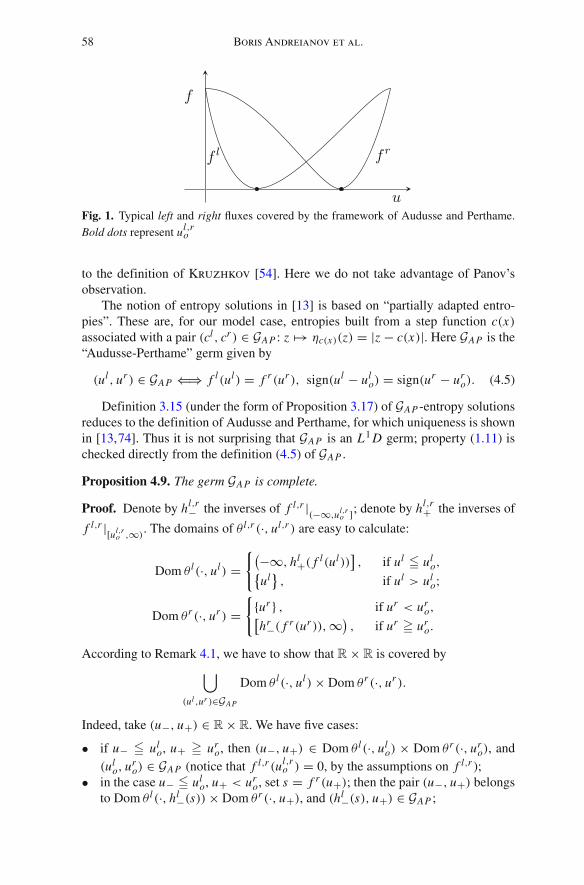
58 Boris Andreianov et al.
Fig. 1. Typical left and right fluxes covered by the framework of Audusse and Perthame.Bold dots represent ul,r
o
to the definition of Kruzhkov [54]. Here we do not take advantage of Panov’sobservation.
The notion of entropy solutions in [13] is based on “partially adapted entro-pies”. These are, for our model case, entropies built from a step function c(x)associated with a pair (cl , cr ) ∈ GAP : z �→ ηc(x)(z) = |z − c(x)|. Here GAP is the“Audusse-Perthame” germ given by
(ul , ur ) ∈ GAP ⇐⇒ f l(ul) = f r (ur ), sign(ul − ulo) = sign(ur − ur
o). (4.5)
Definition 3.15 (under the form of Proposition 3.17) of GAP -entropy solutionsreduces to the definition of Audusse and Perthame, for which uniqueness is shownin [13,74]. Thus it is not surprising that GAP is an L1 D germ; property (1.11) ischecked directly from the definition (4.5) of GAP .
Proposition 4.9. The germ GAP is complete.
Proof. Denote by hl,r− the inverses of f l,r |
(−∞,ul,ro ]; denote by hl,r
+ the inverses of
f l,r |[ul,ro ,∞)
. The domains of θ l,r (·, ul,r ) are easy to calculate:
Dom θ l(·, ul) ={(−∞, hl+( f l(ul))
], if ul � ul
o,{ul
}, if ul > ul
o;
Dom θr (·, ur ) ={
{ur } , if ur < uro,[
hr−( f r (ur )),∞), if ur � ur
o.
According to Remark 4.1, we have to show that R × R is covered by⋃(ul ,ur )∈GAP
Dom θ l(·, ul)× Dom θr (·, ur ).
Indeed, take (u−, u+) ∈ R × R. We have five cases:
• if u− � ulo, u+ � ur
o, then (u−, u+) ∈ Dom θ l(·, ulo) × Dom θr (·, ur
o), and(ul
o, uro) ∈ GAP (notice that f l,r (ul,r
o ) = 0, by the assumptions on f l,r );• in the case u− � ul
o, u+ < uro, set s = f r (u+); then the pair (u−, u+) belongs
to Dom θ l(·, hl−(s))× Dom θr (·, u+), and (hl−(s), u+) ∈ GAP ;
On Scalar Conservation Laws with Discontinuous Flux 59
• the same is true if u− > ulo, u+ < ur
o and f l(u−) � f r (u+) = s;• in the case u− > ul
o, u+ � uro, set s = f l(u−); then the pair (u−, u+) belongs
to Dom θ l(·, u−)× Dom θr (·, hr+(s)), and (u−, hr+(s)) ∈ GAP ;• the same is true if u− > ul
o, u+ < uro and s = f l(u−) � f r (u+).
Hence, (u−, u+) ∈ Dom θ l(·, ul)× Dom θr (·, ur ) for some (ul , ur ) ∈ GAP .��
Notice that Propositions 4.9 and 4.5(i) imply that the maximal L1 D extension(GAP )
∗ of the germ GAP coincides with its closure G AP . The above analysis gives
G AP = GAP ∪{(ul , ur )
∣∣ f l(ul) = f r (ur ), ul > ulo, ur < ur
o
}≡
{(ul , ur )
∣∣ f l(ul) = f r (ur ), sign−(ul − ulo) sign+(ur − ur
o) � 0}.
Now, consider the germ G(ulo,u
ro)
:= {(ul
o, uro)
}. We find that
(G(ul
o,uro)
)∗ =G AP , so
(G(ul
o,uro)
)∗is an L1 D germ; by Proposition 3.4(v), G(ul
o,uro)
is a defi-
nite germ. By Remark 3.12(ii), G(ulo,u
ro)
-entropy solutions of (1.7) coincide withGAP -entropy solutions, thus they coincide with entropy solutions in the sense of
Audusse and Perthame [13]. The completeness of(G(ul
o,uro)
)∗follows from Prop-
osition 4.9. The existence of G(ulo,u
ro)
-entropy solutions can be obtained from The-orem 6.4 or from the adapted viscosity method of Theorem 6.3 in Section 6 (seealso [74]).
Moreover, different notions of entropy solution can be considered for the sameconfiguration of fluxes. Indeed, take any pair (A, B) ∈ (−∞, ul
o]× [uro,∞)which
fulfills the Rankine–Hugoniot condition; set
s(A,B) := f l(A) = f r (B).
The germ G(A,B) := {(A, B)} turns out to be definite, and its unique maximalextension
(G(A,B))∗ is given by
(ul , ur ) ∈ (G(A,B))∗
⇐⇒ f l(ul) = f r (ur ) � s(A,B), sign−(ul − A) sign+(ur − B) � 0.(4.6)
In the same way as in Proposition 4.9, we check that(G(A,B))∗ is complete. Clearly,
the choice (A, B) = (ulo, ur
o) discussed above is a particular case. By analogy withthe case considered by Adimurthi et al. [4] (see also [22] and Section 4.8), suchpairs (A, B) will be called (A, B)-connections.
We easily check that (4.6) accounts for all maximal L1 D germs, for the fluxesconsidered in this paragraph. The monotonicity condition on f l,r can be relaxed,allowing for non-strictly monotone on (−∞, ul,r
o ] and on [ul,ro ,∞) fluxes f l,r .
We see that the definition of entropy solutions due to Audusse and Perthame[13], as applied to the model case (1.7), corresponds to one among infinitely manychoices of L1-contractive semigroups of solutions. Each semigroup is most con-cisely determined by a choice of an (A, B)–connection, that is, by a singleton{(A, B)} from the set (−∞, ul
o] × [uro,∞); any such singleton is a definite germ
with complete dual.
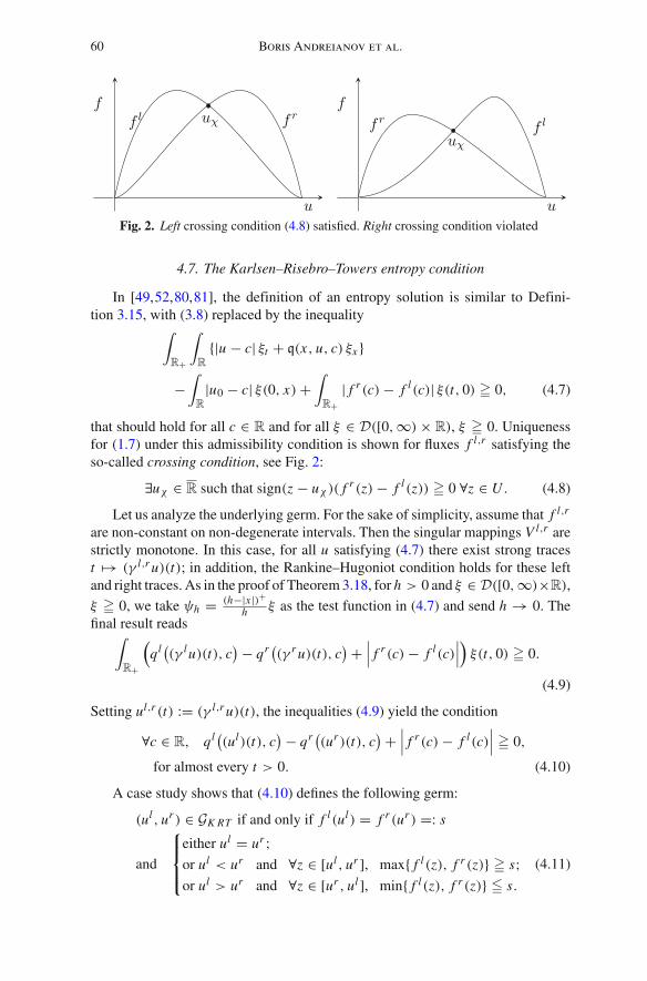
60 Boris Andreianov et al.
Fig. 2. Left crossing condition (4.8) satisfied. Right crossing condition violated
4.7. The Karlsen–Risebro–Towers entropy condition
In [49,52,80,81], the definition of an entropy solution is similar to Defini-tion 3.15, with (3.8) replaced by the inequality∫
R+
∫R
{|u − c| ξt + q(x, u, c) ξx }
−∫
R
|u0 − c| ξ(0, x)+∫
R+| f r (c)− f l(c)| ξ(t, 0) � 0, (4.7)
that should hold for all c ∈ R and for all ξ ∈ D([0,∞)× R), ξ � 0. Uniquenessfor (1.7) under this admissibility condition is shown for fluxes f l,r satisfying theso-called crossing condition, see Fig. 2:
∃uχ ∈ R such that sign(z − uχ )( f r (z)− f l(z)) � 0 ∀z ∈ U . (4.8)
Let us analyze the underlying germ. For the sake of simplicity, assume that f l,r
are non-constant on non-degenerate intervals. Then the singular mappings V l,r arestrictly monotone. In this case, for all u satisfying (4.7) there exist strong tracest �→ (γ l,r u)(t); in addition, the Rankine–Hugoniot condition holds for these leftand right traces. As in the proof of Theorem 3.18, for h > 0 and ξ ∈ D([0,∞)×R),
ξ � 0, we take ψh = (h−|x |)+h ξ as the test function in (4.7) and send h → 0. The
final result reads∫R+
(ql((γ lu)(t), c
) − qr ((γ r u)(t), c) +
∣∣∣ f r (c)− f l(c)∣∣∣) ξ(t, 0) � 0.
(4.9)
Setting ul,r (t) := (γ l,r u)(t), the inequalities (4.9) yield the condition
∀c ∈ R, ql((ul)(t), c) − qr ((ur )(t), c
) +∣∣∣ f r (c)− f l(c)
∣∣∣ � 0,
for almost every t > 0. (4.10)
A case study shows that (4.10) defines the following germ:
(ul , ur ) ∈ GK RT if and only if f l(ul) = f r (ur ) =: s
and
⎧⎪⎨⎪⎩
either ul = ur ;or ul < ur and ∀z ∈ [ul , ur ], max{ f l(z), f r (z)} � s;or ul > ur and ∀z ∈ [ur , ul ], min{ f l(z), f r (z)} � s.
(4.11)
On Scalar Conservation Laws with Discontinuous Flux 61
This definition of GK RT is valid also if f l,r are allowed to degenerate (becomeconstant on intervals). The germ GK RT is closed.
Proceeding as in the proof of Theorem 3.18, we have
Remark 4.10. A function u is an entropy solution of (1.7) in the sense of [52] ifand only if it is a solution in the sense of Definition 3.8 with G∗ replaced by GK RT .Thus, any function of the form (RPb-sol.) with intermediate states (ul , ur ) ∈ GK RT
is a solution of the Riemann problem (1.7), (1.8) in the sense of [52].
Let us show that the crossing condition (4.8) is sufficient for the germ GK RT tobe L1 D and, moreover, maximal L1 D.
Proposition 4.11.
(i) The germ GK RT admits no non-trivial L1 D extension.(ii) If the fluxes f l,r satisfy the crossing condition (4.8), then the germ GK RT is
L1 D (and therefore it is maximal L1 D).
Proof. (i) Assume that there exists (ul , ur ) /∈ GK RT such that GK RT ∪ {(ul , ur )
}is L1 D. We can assume that ul < ur and that there exists z ∈ (ul , ur ) such thatboth f l(z) and f r (z) are strictly smaller than s := f l,r (ul,r ) (the other case issymmetric). We claim the
∃(ul , ur ) ∈ GK RT such that ul < ul � ur < ur and f l,r (ul,r ) < s. (4.12)
Indeed, we can assume that f l(z) � f r (z) < s (the other case is symmetric). Weset s := f r (z) and examine the three possibilities.
– Either f l , f r have a crossing point uχ ∈ [ul , z] such that f l,r (uχ ) � s. Thenit is clear that ul < uχ � z < ur , so that ul,r := uχ satisfies (4.12).
– Or f r > f l on [ul , z]. Set ul,r := inf{ζ ∈ [ul , z] ∣∣ f l,r (ζ ) = s
}. Since f r (z) =
s, ur is well defined and ur � z < ur . Since f l(ul) = s > s � f l(z), ul iswell defined and ul < ul . Because f r > f l and by the choice of ul,r , we haveul < ur , f r (ζ ) � s = f l,r (ul,r ) ∀ζ ∈ [ul , ur ]. Thus (ul , ur ) ∈ GK RT and(4.12) holds.
– Or else, f l,r have a crossing point uχ ∈ [ul , z] with f l,r (uχ ) > s. Thenwe choose the closest to z crossing point uχ with the above property, and setul,r := {
ζ ∈ [uχ , z] ∣∣ f l,r (ζ ) = s}. As in the previous case, we check that
ul,r are well defined, moreover, ul < ur and f r (ζ ) � s = f l,r (ul,r ) for allζ ∈ [ul , ur ]. Thus, (ul , ur ) ∈ GK RT and (4.12) holds.
Now consider the pair (ul , ur ), and the pair (ul , ur )which satisfies (4.12). Theyviolate (1.11); thus GK RT ∪ {
(ul , ur )}
is not L1 D. This contradiction shows thatGK RT has no non-trivial L1 D extension.(ii) Let (ul , ur ), (ul , ur ) be two pairs satisfying the Rankine–Hugoniot condition;set s := f l,r (ul,r ), s := f l,r (ul,r ). Upon exchanging the roles of ul,r and ul,r , weeasily find that (1.11) fails if and only if we have simultaneously s < s, ul > ul ,and ur < ur . These conditions are realized if and only if s < s and
either ul < ul � ur < ur , or ul � ur � ul � ur , or ur � ul < ul � ur ,
or ul � ur < ur � ul , or ur � ul � ur � ul , or ur < ur � ul < ul . (4.13)
62 Boris Andreianov et al.
We check that in all these cases except for the first one and the last one (4.11) neverholds simultaneously for (ul , ur ) and (ul , ur ). In the two cases that were excepted(4.11) can hold simultaneously for (ul , ur ), (ul , ur ) only if the crossing condition(4.8) fails.
This shows that if (4.8) holds, then (1.11) holds for all (ul , ur ), (ul , ur ) ∈GK RT . We conclude that GK RT is an L1 D germ; by (i), it is maximal L1 D. ��
Now let us look at one case where the crossing condition (4.8) fails. Considerthe fluxes in Section 4.6 (that is, of the type in Fig. 1) with ul
o < uro. We claim that
GK RT is not an L1 D germ. Indeed, with the notation of Section 4.6, let
δ = inf{
s∣∣ ∃ u ∈ (ul
o, uro) such that f l(u) = f r (u) = s
};
then for all s ∈ (0, δ], the pair (ul , ur ) := (hl−(s), hr+(s)) belongs to GK RT . Also(ul , ur ) := (ul
o, uro) ∈ GK RT , but then (1.11) is violated. Another way to prove
that GK RT is not L1 D is to notice that the definite germ G(ulo,u
ro)
= {(ulo, ur
o)} is
contained within GK RT , but, according to (4.6), (ul , ur ) does not belong to the
unique maximal L1 D extension(G(ul
o,uro)
)∗of G(ul
o,uro)
.
Based on this fact, we can construct a non-uniqueness example for one simplecase where the crossing condition (4.8) fails.
Example 4.12. Consider the fluxes f l,r : z �→ |z − ul,ro | with ul
o < uro. Then
the entropy condition of [52] is not sufficient to single out a unique solutionto the Riemann problem (1.7), (1.8) with (u−, u+) = (ul
0 − s, ur0 + s), for
all s in(0, 1
2 (uro − ul
o)]. Indeed, the result follows by the above analysis and
by Remark 4.10. We have (u−, u+) ∈ GK RT ; thus the function u(t, x) =u− 1l{x<0}+u+ 1l{x>0} is one solution. Because ul,r ∈ Dom θ l,r (·, ul,r
o ), there existsanother solution of the form (RPb-sol.) with intermediate states (ul
o, uro) ∈ GK RT .
In contrast, if we consider the fluxes as in Section 4.6 with ulo > ur
o such thatthe crossing condition (4.8) holds, then there exists a unique crossing point uχ off l and f r , and uχ ∈ (ur
o, ulo). In this case, one easily checks that GK RT coincides
with the complete maximal L1 D germ((G(uχ ,uχ )
)∗. Another very similar exampleis given in Section 4.8.
Let us also look at the configuration of fluxes considered in Section 4.4. In thiscase, irrespective of the crossing condition (4.8), we always have GK RT = GR H ;thus GK RT is a complete maximal L1 D germ. Also in the case f l ≡ f r , GK RT isa complete maximal L1 D germ, because it coincides with the Vol’pert-Kruzhkovgerm GVKr (here, the crossing condition is satisfied).
Finally, we point out that the germ GK RT is closely related to the “vanishingviscosity” germ GV V which we consider in Section 5; more precisely, we provethere that GV V = GK RT whenever the crossing condition (4.8) holds.
In conclusion, the Definition (4.7) of an entropy solution given in [52] can beequivalently reformulated in terms of the germ GK RT (see Remark 4.10). Wheneverthe crossing condition (4.8) holds, the germ GK RT is maximal L1 D (see Propo-sition 4.11) and the unique entropy solution in the sense (4.7) coincides with theunique GK RT -entropy solution (see [52] or Theorem 3.11 for the uniqueness proof).
On Scalar Conservation Laws with Discontinuous Flux 63
For general fluxes, uniqueness may fail, as in Example 4.12; nevertheless, the cross-ing condition (4.8) is not necessary for the uniqueness of GK RT -entropy solutions.
4.8. Bell-shaped fluxes
Many works have been devoted to the case of bell-shaped fluxes. To fix theideas,∣∣∣∣∣∣∣∣
let U = [0, 1]; assume f l,r : U �→ R+ are such that f l,r (0) = 0 = f l,r (1),f l,r are non-decreasing on [0, ul,r
o ] and non-increasing on [ul,ro , 1],
the graphs of f l , f r have at most one crossing point with abscissa in (0, 1),and if there is a crossing point uχ , then it lies between the points ul
o, uro.
(4.14)
We refer to [22, Figure 1.1] (see also Fig. 2 in the present paper) for a catalogueof different configurations. More general cases with multiple crossing points andoscillating fluxes are considered in [63].
Here the situation is quite similar to the one described in Section 4.6 (we justhave to take into account the fact that ul,r
o are now points of maxima (not min-ima) for f l,r . There exist infinitely many complete maximal L1 D germs. Each ofthese germs contains one and only one pair (A, B) ∈ [ul
o, 1] × [0, uro] (see Prop-
osition 4.6). The germ is thus uniquely determined by a choice of the connection(A, B) (see Adimurthi et al. [4] and Bürger et al. [22]); each maximal L1 Dgerm is the dual
(G(A,B))∗ of the definite germ
G(A,B) :={(A, B): A ∈ [ul
o, 1], B ∈ [0, uro], and f l(A) = f r (B) =: s(A,B).
}We have
(ul , ur ) ∈ (G(A,B))∗ ⇐⇒f l(ul) = f r (ur ) � s(A,B), sign+(ul − A) sign−(ur − B) � 0. (4.15)
As in Proposition 4.9, one shows that (G(A,B))∗ is complete. Another way is to
use Proposition 3.23 together with the existence result of [22]. Indeed, in view ofProposition 3.17, it is clear that Definition 3.15 of G(A,B)-entropy solution is equiv-alent to the definition given by Bürger et al. [22], which requires that inequality(3.8) holds
— for all ξ ∈ D([0,∞)×R), ξ � 0, such that ξ(0, t) = 0; with (cl , cr ) arbitrary;— for all ξ ∈ D([0,∞)× R), ξ � 0, and (cl , cr ) = (A, B).
The technical genuine nonlinearity restriction on f l,r imposed in [22] can bebypassed.5 In Section 6, we give alternative proofs of existence of G(A,B)-entropysolutions, using an adapted viscosity approach and a specific numerical scheme.
5 In works on conservation laws with interface coupling, such as the discontinuous fluxproblems, there are two reasons to ask for the genuine nonlinearity of the fluxes. Firstly,this assumption simplifies the manipulation of the interface fluxes (see Remarks 2.2, 2.3,where these restrictions are bypassed). Secondly, this assumption yields strong compactnessproperties (see [60] and [70,73]). In [22], the compactness is achieved with the help of localBV estimates; thus the nonlinearity assumption on f l,r can be dropped.
64 Boris Andreianov et al.
Let us point out three specific choices of a connection (A, B). The first oneis (A, B) = (1, 0), which corresponds to the extremal choice s(A,B) = 0. Fur-thermore, we have that G(1,0) = {(1, 0), (0, 0), (1, 1)} (this example is mentioned,for instance by Panov [74]). The other extremal choice is to pick (A, B) corre-sponding to the maximum of s(A,B); in this case, we have either A = ul
o (wheneverf l(ul
o) � f r (uro)) or B = ur
o (whenever f l(ulo) � f r (ur
o)).6 This is the germ
identified by Kaasschietter [48], Ostrov [66], and Adimurthi and VeerappaGowda [2]; the corresponding solutions (which are G(A,B)-entropy solutions in ourvocabulary) have been constructed as limits of various physically relevant regular-izations. In the case where f l and f r have no crossing point with abscissa in (0, 1),the definition of Bachmann and Vovelle [14] also leads to this germ, as well asthe one of Karlsen et al. [52] (see Section 4.7).
Finally, consider the case where the crossing condition (4.8) holds with uχ ∈(0, 1). Then (uχ , uχ ) ∈ [ul
o, 1]× [0, uro]. The germ G(uχ ,uχ ) has a unique maximal
L1 D extension(G(uχ ,uχ ))∗ which coincides with the germ GK RT described in Sec-
tion 4.7. As it was demonstrated by Adimurthi et al. [4], this germ also comesout of the vanishing viscosity approaches of Gimse and Risebro [42,43] and Diehl[34–36]. Section 5 below is devoted to a detailed study of the “vanishing viscosity”germ(s).
4.9. The case f l ≡ f r and the Colombo–Goatin germs
Colombo and Goatin [31] consider the conservation law of the form (1.7)with f l = f = f r , which is a bell-shaped function in the sense of Section 4.8;for some F ∈ [0,max f ], the restriction on the value of the flux, | f (u(t, 0))| � F ,is imposed. Starting from a regularization of the constraint and using the entropyformulation of Karlsen et al. [52], the authors obtain a definition of entropysolution which leads to well-posedness in the BV framework.
Analyzing the definition of [31], we easily determine the pairs (ul , ur ) for whichthe elementary solution (1.10) is an entropy solution in the sense of [31]. The set ofall these pairs is, in fact, a maximal L1 D germ; moreover, this germ is the uniquemaximal extension
(GFCG
)∗of the definite “Colombo–Goatin” germ GF
CG :
GFCG = {
(A, B): A, B are determined by A � B, f (A) = f (B) = F}.
This can be seen as an (A, B)-connection of [22] and Section 4.8, except that weare in the particular “degenerate” situation with f l ≡ f r .
In fact, in [31] the constraint F depends on t . This case can be included in ourconsideration. We refer to Remark 3.29 and the forthcoming papers [9,10].
6 We authorize f l,r to be constant on non-degenerate intervals, therefore ul,ro are not
uniquely defined. But all the germs G(ulo,B)
(or G(A,uro)
) corresponding to different choices
of ul,ro have the same closure.
On Scalar Conservation Laws with Discontinuous Flux 65
5. The vanishing viscosity germ
There are many possibilities for introducing a vanishing viscosity regulariza-tion of (1.7). Gimse and Risebro [42,43] recast (1.7) as a 2 × 2 system and addthe simplest viscosity terms to both equations. Diehl [34–36] introduces both theviscosity εuxx and a smoothing fδ of the discontinuity in f; the same approach ispursued in [22]. The regularization term of Kaasschietter [48] is more involved,making appear a capillarity pressure function; the admissibility condition he obtainsis different from the ones of [34–36,42,43].
We shall first study the pure vanishing viscosity regularization of (1.7), that is,
ut + f(x, u)x = εuxx , f(x, z) ={
f l(z), x < 0,
f r (z), x > 0.(5.1)
We pursue the traveling-wave approach of Gelfand [41] (see Section 4.3), whichis, in our context, a “standing-wave” approach. Given f l,r , define the “standing-wave vanishing viscosity” germ by
(ul , ur ) ∈ GsV V ⇐⇒
⎧⎨⎩
there exists a function W : R → R such thatlimξ→−∞ W (ξ) = ul , limξ→∞ W (ξ) = ur , anduε(t, x) = W (x/ε) solves (5.1) in D′(R+ × R).
(5.2)
Clearly, if (ul , ur ) ∈ GsV V , then the elementary stationary solution (1.10) can be
obtained as the almost everywhere and L1loc limit of a sequence of solutions of the
regularized equation (5.1).It turns out that Gs
V V can be replaced by a smaller germ which is describedexplicitly; moreover, we show that Gs
V V is definite. The proposition below leadsto a definition of the maximal L1 D germ GV V , which has already appeared in thework of Diehl [37].
Proposition 5.1. Consider the germ GoV V defined as the set of all the pairs (ul , ur )
such that
f l(ul) = f r (ur ) =: s, and⎧⎪⎪⎪⎪⎪⎪⎨⎪⎪⎪⎪⎪⎪⎩
either ul = ur ;or ul < ur and either f l(z) > s for all z ∈ (ul , ur ],
or f r (z) > s for all z ∈ [ul , ur );or ul > ur and either f l(z) < s for all z ∈ [ur , ul),
or f r (z) < s for all z ∈ (ur , ul ].
(5.3)
(i) The germ GoV V is L1 D.
66 Boris Andreianov et al.
(ii) The closure GoV V of Go
V V is a maximal L1 D germ, and (ul , ur ) ∈ GoV V ⇐⇒
f l(ul) = f r (ur ) =: s, and⎧⎪⎪⎪⎪⎪⎪⎪⎪⎪⎪⎨⎪⎪⎪⎪⎪⎪⎪⎪⎪⎪⎩
either ul = ur ;or ul < ur and there exists uo ∈ [ul , ur ]
such that f l(z) � s for all z ∈ [ul , uo]and f r (z) � s for all z ∈ [uo, ur ];
or ul > ur and there exists uo ∈ [ur , ul ]such that f r (z) � s for all z ∈ [ur , uo]and f l(z) � s for all z ∈ [uo, ul ].
(5.4)
(iii) We have GoV V ⊂ Gs
V V ⊂ GoV V .
(iv) Both GsV V and Go
V V are definite germs with the same unique maximal L1 D
extension GoV V . The Gs
V V , GoV V , and Go
V V entropy solutions coincide.
Definition 5.2. In the sequel, we denote by GV V the maximal L1 D germ GoV V
given by (5.4). We call it the “vanishing viscosity” germ associated with the pairof functions f l,r .
Whenever the dependence on f l,r should be indicated explicitly, we denote
the corresponding vanishing viscosity germ by G f l,r
V V . In [10], we will study more
carefully the dependence of G f l,r
V V on f l,r .
Remark 5.3. (i) Definition 5.2 allows for general continuous fluxes f l,r . Yet itis clear that the so defined germ GV V need not be complete. For instance, ifthe ranges of f l,r do not intersect, GV V is empty and no GV V entropy solutionexists.
(ii) Based on different viscosity approaches, Gimse and Risebro, and then Diehl,have implicitly introduced the set of all admissible elementary solutions of(1.7). These are the elementary solutions used to construct a Riemann solverbased on the “minimal jump condition” [42,43] or on the “�-condition”[34–36]. In fact, both approaches lead to the same germ which coincides withGV V ; the closure operation accounts for the difference between the minimaljump condition and the �-condition. For certain configurations of the fluxesf l,r , a Riemann solver was defined for all data in [34–37,42,43]. In all thesecases we conclude that GV V is complete.
(iii) Diehl [37] reformulated the �-condition from his previous works [34–36]in the following form: the pair (ul , ur ) satisfies the �-condition if
f l(ul) = f r (ur ) and there exists uo ∈ ch(ul , ur ) such that
(ur − uo) ( f r (z)− f r (ur )) � 0, ∀z ∈ ch(ur , uo) (5.5)
(uo − ul)( f l(z)− f l(ul)) � 0, ∀z ∈ ch(ul , uo),
where for a, b ∈ R, ch(a, b) denotes the interval [min{a, b},max{a, b}].Clearly, (5.4) coincides with (5.5). The descriptions (5.4) and (5.5) are remi-niscent of the Oleınik admissibility condition (for convex fluxes f l,r ) and of
On Scalar Conservation Laws with Discontinuous Flux 67
the “chord condition” (see [27,41,44]); as is the case with the chord condition,(5.4) and (5.5) are derived from the travelling-waves approach of [41].
Proof of Proposition 5.1. (i) The proof is entirely similar to the one of Proposi-tion 4.11(ii). Because f l,r are continuous, each of the six cases in (4.13) turns outto be incompatible with the assumption that both (ul , ur ) and (ul , ur ) fulfill (5.3).
Notice that a less tedious proof can be obtained by passing to the limit as ε → 0in the Kato inequality which holds for equation (5.1) [indeed, recall that (1.11) fol-lows from the Kato inequality (1.5)]. Such a proof is given in [11], for the case ofLipschitz continuous f l,r . The general case follows by approximation.
(ii) Recall that we denote by GV V the set of all pairs satisfying (5.4). In a firststep, we show that GV V ⊂ Go
V V . Since GoV V is an L1 D germ by (i) and Proposi-
tion 4.4(i), this implies that GV V is an L1 D germ.Then in a second step, we show that GV V contains the dual
(GoV V
)∗ of GoV V .
According to Propositions 4.4 and 3.4, this yields the reverse inclusion GV V ⊃ GoV V
and hence the maximality of the L1 D germ GV V = GoV V .
We will make repeated use of the continuity of f l,r , without mentioning it.Step 1. Let (ul , ur ) ∈ GV V . If ul = ur , then (ul , ur ) ∈ Go
V V ⊂ GoV V . The remaining
cases are symmetric; let us treat the one with ul < ur .Take s and uo as introduced in (5.4). Consider the function f l(·) − s on the
interval [uo, ur ). If it has a zero point, set zl := min{z ∈ [uo, ur )
∣∣ f l(z) = s}
andzr := min
{z ∈ [zl , ur ] ∣∣ f r (z) = s
}(since f r (ur ) = s, zr is well defined). By
construction and by (5.4), we have
— ul � zl , f l(ul) = f l(zl) = s, and f l � s on [ul , zl ];— zl � zr , f l(zl) = f r (zr ) = s, and f r > s on the interval (zl , zr );— zr � ur , f r (zr ) = f r (ur ) = s, and f r � s on [zr , ur ].
This means that (ul , zl) (respectively, (zr , ur )) is a left contact shock (respec-tively, a right contact shock), and (zl , zr ) ∈ Go
V V .Now consider the situation in which f l(·) − s has no zero point on the
interval [uo, ur ). Then f l � s on [ul , ur ]. In the case f l(ur ) = s, (ul , ur )
is a left contact shock and (ul , ur ) ∈ GoV V . Otherwise, we define zl :=
max{z ∈ [ul , ur )
∣∣ f l(z) = s}. In this case, (ul , zl) is a left contact shock. In addi-
tion, (zl , ur ) ∈ GoV V because zl < ur , f l(zl) = f r (ur ) = s, and f l > s on
(zl , ur ].In all the cases, by definition of the closure, we conclude that (ul , ur ) ∈ Go
V V .Step 2. It suffices to show that if f l(ul) = f r (ur ) but (ul , ur ) /∈ GV V , then thereexists (cl , cr ) ∈ Go
V V such that
ql(ul , cl) < qr (ur , cr ). (5.6)
Set s := f l,r (ul,r ). As before, it suffices to consider the case ul < ur . Define
zl := sup{
z ∈ [ul , ur ] ∣∣ f l � s on [ul , z]},
zr := inf{
z ∈ [ul , ur ] ∣∣ f r � s on [z, ur ]}.
68 Boris Andreianov et al.
If zl � zr , then (5.4) holds with uo = zl , so that (ul , ur ) lies in GV V . Thus, zl < zr .Now, there are three cases to be investigated:
(a) f l and f r have a crossing point zo in the interval (zl , zr ) such that f l,r (zo) < s;(b) f l and f r have a crossing point zo in the interval (zl , zr ) such that f l,r (zo) � s;(c) either f l < f r on the interval (zl , zr ), or f r < f l on the interval (zl , zr ).
In case (a), setting (cl , cr ) := (zo, zo)we obtain (5.6), because ul < cl , cr < ur ,and f l,r (ul,r ) > f l,r (zo). Notice that we do have (zo, zo) ∈ Go
V V .In case (b), by definition of zl,r , there exists s < s such that s belongs to
f l([zl , zo]) ∩ f r ([zo, zr ]). In this case, set cl := max
{z ∈ [zl , zo] ∣∣ f l(z) = s
}and cr := min
{z ∈ [zo, zr ] ∣∣ f r (z) = s
}. We then have (5.6) for the very same
reasons as in case (a). In addition, (cl , cr ) ∈ GoV V , because cl < cr and f l > s on
(cl , zo], f r > s on [zo, cr ).In case (c), the two situations are similar. Consider, for example the case f l <
f r on (zl , zr ). Choose for cr the point of [zl , zr ] where f r attains its minimumvalue over [zl , zr ] and which is the closest one to zl . By definition of zr , s := f r (cr )
is smaller than s. Because f r (zl) � f l(zl) = s > s, we have cr > zl ; in turn, thisyields f l(cr ) < f r (cr ) = s. Since f l(zl) = s > s, there exists cl in the interval(zl , zr ) such that f l(cl) = s. The pair (cl , cr ) fulfills (5.4). In addition, by thedefinition of cr we have f r � s on [zl , zr ] ⊃ [cl , cr ]; thus (cl , cr ) ∈ Go
V V .In all cases, we have constructed (cl , cr ) ∈ Go
V V with property (5.6).The contradiction shows that
(GoV V
)∗ ⊂ GV V . Thus (ii) follows.(iii) We first show the inclusion Go
V V ⊂ GsV V . Let (ul , ur ) satisfy (5.3). In the
case ul = ur , the standing-wave profile W can be chosen constant on R. The fourother cases are symmetric. For instance, in the case ul < ur and f l(z) > s for allz ∈ (ul , ur ], W is a continuous function that is constant (equal to ur ) on [0,∞).On the interval (−∞, 0], W is constructed as a solution of the autonomous ODE
W ′ = f l(W )− f l(ul), W (0) = ur .
Indeed, because f l(W )− f l(ul) = f l(W )− s > 0 for W taking values in (ul , ur ],W is non-decreasing. If the graph of W crosses the line W = ul , we extend thesolution by the constant value ul on the left from the crossing point. Otherwise, Wis defined on the whole interval (−∞, 0], and there exists d := limξ→−∞ W (ξ) ∈[ul , ur ]. In this case, f l(d)− s = 0, which yields d = ul . Therefore (5.2) holds.
Next, we show that GsV V ⊂ Go
V V . Let (ul , ur ) ∈ GsV V . The case ul = ur is triv-
ial; by a symmetry argument, we can assume ul < ur . The standing-wave profileW in (5.2) is a continuous on R function which is monotone on R− and on R+.Moreover, replacing W by max
{ul ,min {W, ur }}, we still have a standing-wave
profile with the same properties. Then uo := W (0) lies within [ul , ur ]. The mono-tonicity of W guarantees that f l − s � 0 on [ul , uo], and f r − s � 0 on [uo, ur ].Thus (ul , ur ) fits the definition (5.4). By (ii), (ul , ur ) ∈ Go
V V .(iv) The claim follows readily from (ii), (iii), and Proposition 4.4 (iii), (iv).
��Now we compare GV V with the known germs studied in Section 4 and in [34–
37,42,43]. Let us emphasize that in many cases studied in these papers, GV V turns
On Scalar Conservation Laws with Discontinuous Flux 69
out to be complete. The completeness of GV V will be further studied in Theorem 6.1(see Section 6).
Remark 5.4. (i) With the help of the characterizations (4.11), (5.3), (5.4) ofGK RT , Go
V V , and GV V , respectively, we easily see that GoV V ⊂ GK RT = GV V
whenever the crossing condition (4.8) holds. In this case, the GV V and GK RT
entropy solutions coincide.(ii) Consider the case of bell-shaped fluxes (4.14) treated in Section 4.8.
— First assume uro � ul
o and that there exists a crossing point uχ ∈ [uro, ul
o]between f l and f r (in this case, the crossing condition (4.8) holds).Then GV V contains the definite germ G(uχ ,uχ ). Thus the G(uχ ,uχ ), GV V ,
and GK RT entropy solutions coincide. In addition, since(G(uχ ,uχ ))∗ is
complete, GV V is complete.— If, on the other hand, a crossing point uχ exists but ul
o � uχ � uro (this is
the “bad crossing” case), then the GV V -entropy solutions coincide withthe entropy solutions for the germ G(A,B) with (A, B) corresponding tos(A,B) = smax, where
smax := max{
s ∈ R+ | ∃(A, B) ∈ [ulo, 1] × [0, ur
o] s.t. f l (A) = f r (B) = s}.
(5.7)
Also in the case where the fluxes do not cross within (0, 1), GV V = G(A,B)with s(A,B) = smax. In both cases, GV V is complete because
(G(A,B))∗ iscomplete. Let us stress that in the non-crossing case, GK RT coincides withGV V , whereas in the case of a “bad crossing”, GK RT \ GV V �= ∅.
In conclusion, following Diehl [34–36] and Bürger et al. [22], let us men-tion that the germ Go
V V also arises from the more general regularization-viscosityapproach
ut + fδ(x, u)x = εuxx in D′(R+ × R), (5.8)
where fδ is a continuous (in x) approximation to f.
Proposition 5.5. Suppose f l,r are locally Lipschitz continuous. Let (fδ(·, ·))δ>0 bea family of continuous functions approximating f in (1.7) in the following sense:
– fδ(x, z) is of the form F(x/δ, z) with some fixed function F;– for all y ∈ R, there exists αy ∈ [0, 1] such that F(y, ·) = αy f l(·) + (1 −αy) f r (·);
– for y � −1, αy = 1 (that is, F(y, ·) ≡ f l(·)); similarly, for y � 1, F(y, ·) ≡f r (·).
Let (ul , ur ) ∈ GoV V . Denote by L the Lipschitz constant of f l,r on the interval
between ul and ur .Then, whenever δ/ε � 2/L, there exists a stationary solution u(t, x) = uε,δ(x)
of (5.8) satisfying limx→−∞ uε,δ(x) = ul , limx→∞ uε,δ(x) = ur . In addition, asε ↓ 0, with 0 < δ � 2
L ε, uε,δ converges almost everywhere on R and in L1loc(R) to
the elementary stationary solution ul1l{x<0} + ur 1l{x>0} of (1.7).
70 Boris Andreianov et al.
Proof. Let (ul , ur ) ∈ GoV V . The case ul = ur is trivial since constants solve (5.8).
The other cases are symmetric, so let us consider only the one with ul < ur andf l > s on the interval (ul , ur ].
Setting y = x/δ, uε,δ(x) = U (x/δ), we are reduced to the problem
εU ′(y) = δ (F(y,U (y))− s), U (−∞) = ul , U (∞) = ur . (5.9)
In view of the assumptions on F and also the ratio δ/ε, the (constant) functionm+ : y ∈ (−∞, 1] �→ ur is a subsolution of the ODE U ′ = δ/ε(F(y,U )− s); andthe function m− : y ∈ (−∞, 1] �→ min{ul , ur +Lδ/ε (y−1)} is a supersolution ofthe same ODE. By the classical ODE existence and comparison result, there existsa solution of the ODE on (−∞, 1] with U (1) = ur , and we have m− � U � m+.In particular, U (·) takes values in (ul , ur ] and satisfies the autonomous equationU ′ = δ/ε( f l(U ) − s) on (−∞,−1). Since by assumption, f l > s on (ul , ur ],U (·) admits a limit as y → −∞ which necessarily equals ul . Finally, extending Uby the constant value ur on [1,∞), we obtain a solution to problem (5.9).
For the proof of convergence of the solutions uε,δ(x) = U (x/δ), we replacem+(·) on (−∞,−1] by the solution V (·) of V ′ = δ/ε( f l(V )− s) with the initialdatum V (−1) = ur ; with the same arguments as above, such a solution exists, ittends to ul as y → −∞, and it bounds U (·) from above. By assumptions, we haveδ � 2ε/L → 0 as ε → 0. For all x < 0, for all sufficiently small ε, the quantity|uε,δ(x) − ul | is upper bounded by |V (x/δ) − ul | which converges to zero. Forx > 0, we simply have uε,δ(x) = ur whenever δ � x . We conclude the pointwiseconvergence of uε,δ to the profile (1.10); since all these functions take values within[ul , ur ], the L1
loc convergence follows. ��
6. Some existence and convergence results
In this section, for a fixed germ G, we study the existence of G-entropy solutionsand convergence of various vanishing viscosity and numerical approximations.
The first result concerns the vanishing viscosity germ GV V , which was describedin Section 5. The main assumption for the existence result is the availability of auniform L∞(R+ × R) estimate for solutions uε of (5.1) with a given initial datumu0 ∈ L∞(R). We also impose some additional nonlinearity and Lipschitz conti-nuity assumptions on the fluxes f l,r . For the sake of simplicity, we restrict ourattention to fluxes satisfying f l,r (0) = 0 = f l,r (1) [the bell-shaped fluxes (4.14)offer one example] and an initial condition u0 with values in [0, 1]; thus solutionsare automatically bounded, because they take values in [0, 1].
Recall that in the setting (4.14) of bell-shaped fluxes with ulo � uχ � ur
o, thegerm GV V coincides with
(G(uχ ,uχ ))∗; the other maximal L1 D germs(G(A,B))∗
are corresponding to other choices of the connection (A, B). For an arbitrary butfixed connection (A, B), using a specially fabricated artificial viscosity we proveconvergence of viscosity approximations to the G(A,B)-entropy solution.
Then we look at a general complete L1 D germ G for a pair of locallyLipschitz continuous functions f l,r . We construct solutions by showing con-vergence of a suitably adapted monotone three-point finite volume scheme. For
On Scalar Conservation Laws with Discontinuous Flux 71
these results, the uniform BVloc estimates away from the interface {x = 0} are ofimportance (see [20,22]). As previously, we need a uniform L∞ bound onthe approximations, which actually comes for free from the completeness of G(see Proposition 3.20).
Finally, we prove convergence of uniformly L∞ bounded (thus weakly com-pact) sequences of approximate G-entropy solutions, without utilizing BV type apriori estimates and assumptions that ensure strong compactness. For this purpose,we have to assume that G is a maximal L1 D germ for which existence is alreadyknown (see Section 1.4). Then, assuming that the approximation procedure is com-patible with the germ G (that is, that the elementary stationary solutions selectedby the germ G are obtained as limits of the approximation) and that an appropriateKato inequality holds for the approximate solutions, we deduce the convergenceof the approximating procedure.
6.1. The standard vanishing viscosity approach
To be specific, let us work with the vanishing viscosity germ GV V in Defini-tion 5.2, and note that according to Proposition 5.1(iv), we can replace GV V byGs
V V or by GoV V .
Theorem 6.1. Suppose f l,r : [0, 1] −→ R are Lipschitz continuous functions thatare not affine on any interval I ⊂ [0, 1]. Moreover, assume f l,r (0) = 0 = f l,r (1).Then for all u0 which is measurable and takes values in [0, 1], there exists a uniqueGV V -entropy solution to problem (1.7),(1.2). In particular, the germ GV V is def-inite and complete. In addition, the GV V -entropy solutions are the vanishing vis-cosity limits in the following sense. For each ε > 0, there exists a weak solutionuε ∈ L2
loc(R+; H1loc(R)) of the viscous problem (5.1) with any measurable initial
data uε|t=0 = uε0 taking values in [0, 1]. If we moreover assume uε0 → u0 almosteverywhere on R, then uε converge almost everywhere on R+ × R to the uniqueGV V -entropy solution of (1.7), (1.2).
A multi-dimensional analogue of Theorem 6.1 holds, see [10,11].
Remark 6.2. (i) The assumptions f l,r (0) = 0 = f l,r (1) and uε0(x) ∈ [0, 1]are put forward to ensure that the family (uε)ε>0 is bounded in L∞. Indeed,Theorem 6.1 remains true if the L∞ bound is provided by some other means.This boundedness assumption is important. For example, in situations wherethe graphs of f l and f r do not intersect, it is then clear that (1.7) has nosolution and consequently ‖uε‖∞ → ∞ as ε → 0.
(ii) On the contrary, the Lipschitz continuity assumption on f l,r is needed onlyto establish the existence of a solution semigroup for viscous problem (5.1)that satisfies the Kato inequality. This assumption can be bypassed, thanks toa regularization of f l,r . We then establish the existence of a (possibly non-unique) solution uε to (5.1), (1.2) with merely continuous functions f l,r , andthe convergence of the sequence (uε)ε>0 to the unique GV V -entropy solutionof problem (1.7), (1.2).
72 Boris Andreianov et al.
(iii) As pointed out in Corollary 6.6, the assumption of non-degeneracy of f l,r
imposed in Theorem 6.1 can be dropped; but the proof becomes much moreindirect, involving a beforehand justification of the existence of GV V -entropysolutions (for this, we use a numerical scheme, see Theorem 6.4). Moreover,in Corollary 6.6 we do not prove that the germ GV V is complete, but we takecompleteness as a hypothesis.
Proof of Theorem 6.1. Extend f l,r by zero outside [0, 1]. Let T denote a genericpositive number. The following a priori estimate is easily obtained:
∫R
1
2
(uε(T, ·))2 + ε
∫ T
0
∫R
|uεx |2
�∫
R
1
2
(uε(0, ·))2
+∫ T
0
∫ 0
−∞
(∫ uε
0f l(z) dz
)x
+∫ T
0
∫ ∞
0
(∫ uε
0f r (z) dz
)x
� C(T, ‖uε0‖2, f l,r ), (6.1)
where uε ∈ C(R+; H1(R)) is a solution of (5.1). Thanks to this estimate, it canbe shown by the classical Galerkin technique (see, for example Lions [59]) thatfor any ε > 0 and uε0 ∈ L2(R) there exists a solution uε ∈ C(R+; H1(R))
to the Cauchy problem for the parabolic equation (5.1). What’s more, the Katoinequality holds for (5.1). Indeed, assuming (uε0 − uε0)
+ belongs to ∈ L1(R), letuε, uε ∈ L2
loc(R+; H1loc(R)) be two weak solutions of (5.1) corresponding to the
initial data uε0, uε0 ∈ L∞(R), respectively. For α < 0, let us introduce a Lipschitzcontinuous approximation Hα of the sign+(·) function:
Hα(z) := min
{z+
α, 1
}, z ∈ R, (6.2)
and use the test function Hα(uε−uε) ξ , ξ ∈ D([0,∞)×R), in the weak formulationof (5.1). Notice that, due to the Lipschitz assumption on f l ,∣∣∣∣
∫R+
∫R−
(f l(uε)− f l(uε)
) (Hα)
′(uε − uε) (
uε − uε)
x ξ
∣∣∣∣� ‖( f l)′‖L∞‖ξ‖L∞
∫∫{0<uε−uε<α}
∣∣(uε − uε)
x
∣∣ −→ 0 as α → 0,
thanks to (6.1); and the same holds with R−, f l replaced with R+, f r . Hence asα → 0, we deduce the Kato inequality: for all ξ ∈ D([0,∞)× R), ξ � 0,∫
R+
∫R
((uε − uε)+ξt + q+(x, uε, uε)ξx
)+
∫R
(uε0 − uε0)+ξ(0, ·) � ε
∫R+
∫R
[(uε − uε)+
]x ξx ; (6.3)
On Scalar Conservation Laws with Discontinuous Flux 73
where we have written q+ for the semi-Kruzhkov entropy flux:
q+(x, z, k) := sign+(z − k)(( f l(z)− f l(k))1l{x<0} + ( f r (z)− f r (k))1l{x>0}
).
In this inequality, using, for example the technique of Maliki and Touré [62] wecan let ξ converge to the characteristic function of [0, T ) × R in such a way thatthe terms with ξx vanish as ε → 0. Then we get the L1 contraction and comparisoninequality
for almost every t > 0,∫
R
(uε − uε)+(t) �∫
R
(uε0 − uε0)+. (6.4)
Inequality (6.4) ensures the uniqueness of a weak solution in L2loc(R+; H1
loc(R))
of the Cauchy problem for the parabolic equation (5.1). It also yields the compari-son principle. Keeping in mind that, under our assumptions, the constants 0 and 1are evident solutions of (5.1), we derive the maximum principle: for data uε0 takingvalues in [0, 1], 0 � uε � 1 holds almost everywhere on R+ × R.
Now we are in a position to extend the existence result for (5.1) to a generalinitial function u0 taking values in [0, 1]. Indeed, following Ammar and Witt-bold [6] we can take the bi-monotone approximation of u0 ∈ L∞(R) by boundedcompactly supported functions, namely,
(u0)m,n := min{(u0)
+, n}
1l{|x |<n} − min{(u0)
−,m}
1l{|x |<m}.
We deduce the existence of a weak solution to (5.1). Moreover, thanks to themonotone convergence theorem, the obtained solutions still fulfill (6.3) and (6.4).Finally, the solutions belong to L2
loc(R+; H1loc(R)), thus the uniqueness result
applies.Now, let us justify the convergence of uε to a GV V -entropy solution. Take a
sequence of data uε0 as in the statement of the theorem. By the non-degeneracyassumption on f l,r and strong precompactness results of [70,73], applied sepa-rately in the domains {x > 0} and {x < 0}, we deduce that there exists a (notlabelled) sequence ε ↓ 0 such that uε converge to some limit u in L1
loc(R+ × R).By the dominated convergence theorem, we also have the L1
loc convergence of uε0to u0. Passing to the limit in the distributional formulation of the Cauchy problemfor (5.1), we find that u is a weak solution of (1.7), (1.2). Following [54], we alsodeduce the Kruzhkov entropy inequalities in the domains {x > 0} and {x < 0}. Inparticular, the existence of strong traces γ l,r u on {x = 0} follows.
Finally, notice that for any pair u, u obtained as the vanishing viscosity limit withthe same extracted subsequence ε → 0, we can pass to the limit in the Kato inequal-ity (6.3), where the right-hand side vanishes due to a uniform bound on ε|uεx |2 inL1
loc(R+ × R). To conclude the proof, it remains to notice that, by the Definition(5.2) of Gs
V V , the elementary solutions u = cl1l{x<0} + cr 1l{x>0}, (cl , cr ) ∈ GsV V ,
are obtained as vanishing viscosity limits. Passing to the limit in the correspondingKato inequalities written for ε > 0, we infer the entropy inequalities (3.8) with(cl , cr ) ∈ Gs
V V and zero remainder term RG . According to Proposition 3.17 andDefinition 3.15, u is a Gs
V V -entropy solution of (1.7), (1.2). By Proposition 5.1(iv),(GsV V
)∗ coincides with the maximal L1 D germ GV V , thus we conclude that u is the
74 Boris Andreianov et al.
unique GV V -entropy solution of (1.7), (1.2). The uniqueness of the accumulationpoint ensures that all sequences converge to the same limit u.
It remains to notice that we have obtained a solution for every measurable initialfunction u0 with values in U = [0, 1]. In particular, for all Riemann initial data u0in (1.8), there exists a GV V -entropy solution. According to Remark 3.13, the germGV V is complete. ��
6.2. The vanishing viscosity approach adapted to (A, B)-connections
In this section we work with bell-shaped fluxes as defined in (4.14). Recallthat any complete maximal L1 D germ is of the form
(G(A,B))∗, where G(A,B) :={(A, B)} is a definite germ and the connection (A, B) is a pair satisfying
(A, B) ∈ [ulo, 1] × [0, ur
o] and f l(A) = f r (B) =: s(A,B). (6.5)
The explicit description of(G(A,B)
)∗ is given by formula (4.15).Our goal is to construct G(A,B)-entropy solutions by the vanishing viscosity
method; clearly, the choice of viscosity must be adapted to the connection (A, B).For the Buckley–Leverett equation with a flux that is discontinuous at x = 0,Kaasschietter [48] gives a physically motivated viscosity of the form
ε (λ(x, u)pc(u)x )x ,
where pc(·) is the capillary pressure and λ(x, ·) = λl(·)1l{x<0} + λr (·)1l{x>0} isthe mobility function, discontinuous at {x = 0}. This choice corresponds to theparticular connection (A, B) such that s(A,B) = smax, see (5.7).
Our approach is more academic. We fix an arbitrary connection (A, B) andconstruct an artificial “adapted viscosity” of the form
ε (a(x, u))xx
such that the stationary solution c(x) := A1l{x<0} + B1l{x>0} of the limit equa-tion (1.7) is also a solution of the viscous problem
ut + f(x, u)x = εa(x, u)xx ,
f(x, z) ={
f l(z), x < 0,
f r (z), x > 0.a(x, z) =
{al(z), x < 0,
ar (z), x > 0.(6.6)
In the sequel, by a weak solution of (6.6) we mean a function u ∈ L∞(R+ ×R) satisfying (6.6) in the sense of distributions and such that w(·) := a(·, u(·))belongs to L2
loc(R+; H1loc(R)). For (6.6) to be parabolic, the functions al,r should be
strictly increasing on [0, 1]; and it is convenient to ask that inf z∈[0,1](al,r
)′(z) > 0.
Because f l,r (0) = 0 = f l,r (1) by assumption, it is convenient to require the con-stants u ≡ 0 and u ≡ 1 to be solutions of (6.6) for all ε > 0.
For example, any continuous functions al,r such that
al,r are strictly monotone on [0, 1], and
⎧⎪⎨⎪⎩
al(0) = 0 = ar (0),
al(A) = κ = ar (B),
al(1) = 1 = ar (1),
(6.7)
On Scalar Conservation Laws with Discontinuous Flux 75
with κ ∈ (0, 1), do satisfy the above requirements, except with (A, B) = (1, 0), inwhich case we take κ = 0. For example, we can interpolate the values (6.7) to pro-duce piecewise affine and strictly increasing examples of such functions al,r definedon [0, 1]. Notice that, by choosing κ appropriately, for the connection (uχ , uχ ) weobtain the standard viscosity εuxx studied in the previous section; under assumption(4.14), we actually have
(G(uχ ,uχ ))∗ = GV V .Now we will prove that the G(A,B)-entropy solutions of (1.7) can be obtained
as the limits of the vanishing adapted viscosity approximations defined by (6.6).More precisely, we have the following analogue of Theorem 6.1, which representsa reinterpretation and improvement of the results of Bürger et al. [22].
Theorem 6.3. Assume that f l,r are Lipschitz continuous functions of the form(4.14). In addition, assume that f l and f r are not affine on any interval I ⊂ [0, 1].Let (A, B) be a given connection of the form (6.5). Then, for each measurable ini-tial function u0 taking values in [0, 1], there exists a unique G(A,B)-entropy solutionof (1.7), (1.2). Moreover, consider al,r satisfying (6.7) and set
a(x, ·) = al(·)1l{x<0} + ar (·)1l{x>0};assume in addition that
(al,r
)′ � const > 0 almost everywhere on [0, 1]. Let(uε0)ε>0 be a family of measurable functions taking values in [0, 1] such thatuε0 → u0 almost everywhere on R. For each ε > 0, there exists a weak solution uε
of the adapted viscosity regularized problem (6.6) with initial data uε∣∣t=0 = uε0.
The sequence (uε)ε>0 converges almost everywhere on R+ × R to the uniqueG(A,B)-entropy solution of (1.7), (1.2).
Proof. We will focus on the existence of solutions to the adapted viscous problemsand the convergence of these solutions as the viscosity parameter tends to zero.The proof is very similar to the proof of Theorem 6.1. We will argue in terms ofthe unknown w(t, x) := a(x, u(t, x)). Then
u(t, x) = b(x, w(t, x)), b(x, ·) = (al)−1
(·)1l{x<0} + (ar )−1
(·)1l{x>0},and the Cauchy problem for (6.6) is equivalent to
b(x, w)t + f(x, b(x, w))x = εwxx , w(0, x) = wε0 := a(x, uε0(x)). (6.8)
Existence for (6.8) is obtained by proving convergence of Galerkin approximationsalong the lines of Alt and Luckhaus [5]. Indeed, set B(x, r) := ∫ r
0 b(x, z) dz. Inthe same way as for (6.1), assuming that B◦wε0(·) := B(·, wε0(·)) belongs to L1(R)
and using the weak chain rule [5], we obtain the a priori estimate∫R
B(·, wε(T, ·))+ ε
∫ T
0
∫R
|wεx |2
�∫
R
B(·, uε(0, ·))
+∫ T
0
∫ 0
−∞
(∫ uε
0f l(z)al(z) dz
)x
+∫ T
0
∫ ∞
0
(∫ uε
0f r (z)ar (z) dz
)x
� C(
T,∥∥B ◦ wε0
∥∥L1(R)
, f l,r , al,r).
76 Boris Andreianov et al.
This estimate and the compactness technique of [5] ensure the convergence of theGalerkin approximations to a weak solution wε of (6.8) with the properties
B ◦ wε ∈ L∞(R+; L1(R)), wε ∈ L2loc(R+; H1(R)),
(b ◦ wε)t ∈ L2loc(R+; H−1(R)), (b ◦ wε)(0, ·) = b ◦ wε0.
As in the proof of Theorem 6.1, the assumption B ◦ wε0 ∈ L1(R) can be dropped,thanks to the bi-monotone approximation of wε0 by compactly supported boundedfunctions
(wε0)m,n := min{(wε0)
+, n}
1l{|x |<n} − min{(wε0)
−,m}
1l{|x |<m}
(see [6]) and thanks to the comparison principle that we now justify. Indeed, letwε be a solution of the same equation corresponding to the initial datum wε0. Takeξ ∈ D([0,∞) × R), ξ � 0, and Hα given by (6.2). Utilizing the test functionHα(wε − wε)ξ , using the doubling-of-variables technique in time only, as in Otto[68], and taking into account that f l,r and bl,r are Lipschitz continuous (see theproof of Theorem 6.1), we deduce the Kato inequality∫
R+
∫R
((b ◦ wε − b ◦ wε)+ξt + q+(x; b ◦ wε, b ◦ wε) ξx
)+
∫R
(b ◦ wε0 − b ◦ uε0)+ξ(0, ·) � ε
∫R+
∫R
(wεx − wεx ) ξx ;
here q+ has the same meaning as in (6.3). With the technique of [62], we can letξ converge to the characteristic function of [0, T ) × R and derive the contractionand comparison inequality
for almost every t > 0,∫
R
(uε − uε)+(t) �∫
R
(uε0 − uε0)+.
By the definition of (A, B) and assumptions (4.14), (6.7), the constants 0 and 1 areevident solutions of (5.1). Hence, the following maximum principle holds: for datauε0 taking values in [0, 1], we have 0 � uε � 1 almost everywhere on R+ × R.Also the function u(x) := A 1l{x<0} + B 1l{x>0} is an apparent solution of (5.1).As in the proof of Theorem 6.1, we use uniform estimates on uε and compactnessarguments to pass to the limit in the Kato inequality written for uε and for uε ≡ u.What we obtain is the entropy inequality (3.8) with (cl , cr ) = (A, B) and RG = 0(this is exactly the entropy inequality of Bürger et al. [22]). In addition, we seethat u is a weak solution of (1.2), (1.7) and it is a Kruzhkov entropy solution in thedomains {x < 0} and {x > 0}. We conclude either using the uniqueness result of[22], or using Proposition 3.17 and the fact that G(A,B) is definite. ��
6.3. Existence for complete germs through the discretization approach
We now establish the existence of a G-entropy solution for any complete max-imal L1 D germ G. For the sake of simplicity, let us take U = R.
On Scalar Conservation Laws with Discontinuous Flux 77
Theorem 6.4. Let G be a complete maximal L1 D germ. Assume that the func-tions f l,r are locally Lipschitz continuous on R. Then for any initial functionu0 ∈ L∞(R) there exists a unique G-entropy solution of problem (1.2), (1.7).
Proof. The proof is a combination of the well-known finite volume method (seeEymard et al. [38]) with a careful treatment of the interface {x = 0} using theGodunov scheme; the proof of compactness of the family of discrete solutions isbased upon the BVloc estimate of Burger et al. [20,22] and an L∞ bound similarto the one of Proposition 3.20. Note that global (up to the interface) BV estimatesare, in general, not available, see [1].
Recall that by the definition of a complete germ, there exists a Riemann solverRSG at {x = 0}, fully determined by G, defined for all Riemann data (1.8). We setm := ess infR u0 (respectively, M := ess supR u0) and denote by cl,r (respectively,by Cl,r ) the one-sided traces γ l,rRSGm (respectively, γ l,rRSG M) of the solutionof the Riemann problem at {x = 0} with the constant datum u± = m (respectively,with the constant datum u± = M). Assign
bl,r := min{
cl,r ,m}, Bl,r := max
{Cl,r ,M
}. (6.9)
We consider an explicit finite volume scheme based on the uniform spatial mesh⋃i∈Z(i�x, (i + 1)�x), �x > 0,
and a time step �t satisfying the CFL condition
λ := �t
�x� 1/2L, L := max
{max
z∈[bl ,Bl ]
∣∣∣( f l)′(z)∣∣∣ , max
z∈[br ,Br ]∣∣( f r )′(z)
∣∣} .A lower bound for L can be obtained from Proposition 3.20.
For i �= 0, we can utilize any consistent monotone flux gi+1/2(·, ·) (see forexample [38]); but at the interface i = 0 we take gi+1/2(·, ·) to be the Godunovflux based on the exact G-Riemann solver. Given the numerical flux gi+1/2(·, ·),the difference scheme is defined as
uni = un−1
i −λ(
gi+1/2
(un−1
i+1 , un−1i
)− gi−1/2
(un−1
i , un−1i−1
)), ∀n ∈N, ∀i ∈Z.
where the iteration is initialized by
u0i := 1
�x
∫ (i+1)�x
i�xu0, ∀i ∈ Z.
The monotonicity of the numerical flux gi+1/2(·, ·) and the CFL condition ensurethat the scheme can be written as
uni = Hi
(un−1
i−1 , un−1i , un
i+1
), ∀n ∈ N, ∀i ∈ Z,
for some functions Hi (·, ·, ·) that are monotone in each of the three arguments. Weidentify the discrete solution (un
i )n∈N,i∈Z with the piecewise constant function
Shu0 :=∑
n∈N, i∈Z
uni 1l((n−1)�t,n�t)×(i�x,(i+1)�x));
where h is a collective symbol for the discretization parameters �x,�t .
78 Boris Andreianov et al.
By construction (exact G-Riemann solver at the interface {x = 0}),the difference scheme preserves all stationary solutions of (1.7)
of the form cl 1l{x<0} + cr 1l{x>0} with (cl , cr ) ∈ G.(6.10)
First, let us establish the following uniform L∞ bound on Shu0:
b(x) := bl 1l{x<0} + br 1l{x>0}� (Shu0)(t, x)
� Bl 1l{x<0} + Br 1l{x>0} =: B(x), (6.11)
for almost every (t, x) ∈ (0,∞)×R, where bl,r , Bl,r are defined in (6.9). To prove(6.11), we take the Riemann initial datum b(·) and look at the corresponding dis-crete solution (Shb)(�t, ·) after the first time step. Denote by bn
i the values takenby (Shb)(�t, ·). Notice that, by the choice of bl,r , the exact solution RSGb of theRiemann problem has the one-sided traces cl,r at {x = 0}. Therefore, the Godunovflux g1/2(bn
0 , bn1) = g1/2(bl , br ) at the interface at time level n = 1 takes the value
f l,r (cl,r ) (the two values being equal). From the definition of the scheme, it is clearthat b1
i = b0i for all i �= 0, 1. Moreover, from the definition of the scheme we have
b10 = bl − λ
(f l(cl)− f l(bl)
), b1
1 = br − λ(
f r (br )− f r (cr )).
Because bl � cl by construction, and because the state bl at x < 0 can be joinedto the state cl at x = 0− with waves of negative speed for the flux f l , it followsthat f l(cl) � f l(bl). Similarly, we have f r (cr ) � f r (br ). Combining the aboveinformation, we deduce that for all i ∈ Z, b1
i � b0i . Thus we have
(Shb)(�t, ·) � b(·).Hence by induction, using the monotonicity of the scheme, we deduce
(Shb)(t, x) � b(x) for almost every (t, x) ∈ (0,∞)× R.
Because u0 � b almost everywhere on R and again in view of the monotonicity ofthe scheme,
(Shu0)(t, x) � (Shb)(t, x) � b(x) for almost every (t, x) ∈ (0,∞)× R,
which establishes the desired lower bound in (6.11). The proof of the upper boundis entirely similar.
Now we assume that u0 is compactly supported and belongs to BV (R). Thenfor all T > 0 and l > 0, we apply the uniform BV ((0, T )× (R \ (−l, l))) estimateof [20,22] to the family (Shu0)h>0. To establish this estimate, we first combine thediscrete L1 contraction property, obtained from the Crandall-Tartar lemma [33],with the L1 Lipschitz continuity in time t of the solver Sh . The result is an estimateof the time variation of Shu0 on (0, T )×R in terms of the variation Var u0 of the ini-tial data u0 on R. Then, using the mean value theorem, we pick lh ∈ (0, l) such thatthe variation of (Shu0)(·,±lh) does not exceed Const (Var u0) / l. Subsequently,
On Scalar Conservation Laws with Discontinuous Flux 79
we consider (Shu0)|R\(−lh ,lh) as originating from the finite volume discretizationof two Cauchy-Dirichlet problems. For instance on (0, T )× (lh,∞), both the ini-tial condition u0|(lh ,∞) and the boundary condition ub(·) := (Shu0)(·, lh) havethe variation controlled in terms of Var u0 and of 1
l . It follows that the space-timevariation of Shu0 on (0, T )× (R \ (−l, l)) ⊂ (0, T )× (
R \ (−lh, lh))
is boundeduniformly in h; we refer to [20, Lemma 4.2], [22, Lemmas 5.3, 5.4] for the details.Using in addition the L∞ bound, with the help of a diagonal extraction argument,we get convergence as h → 0 of a (not labelled) sequence (Shu0)h to somelimit u.
Now we justify that the limit u is the unique G-entropy solution of (1.2), (1.7).The above BVloc estimates (or the standard “weak BV ” estimates for monotonefinite volume schemes, see [38]) permit us to get an approximate weak formula-tion and pass to the limit as h → 0. It follows that u is a weak solution to (1.2),(1.7). In the same way, the technique of [38] allows us to get the Kruzhkov entropyinequalities for u in the domains {x < 0} and {x > 0}.
According to Definition 3.15 and Proposition 3.17, what remains is to provethe entropy inequality (3.8) with an arbitrary non-negative test function ξ (not nec-essarily zero on the interface {x = 0}) and with any pair (cl , cr ) ∈ G. Let us givea proof using (6.10). To this end, notice that a key feature of the scheme, thanks tothe use of the Godunov flux of the exact G-Riemann solver at the interface, is thatthe discrete solutions uh := Shu0 take the values
(γ luh)(·) ≡∑
n∈Nun
0 1l((n−1)�t,n�t),
(γ r uh)(·) ≡∑
n∈Nun
1 1l((n−1)�t,n�t)
at the interface (strong one-sided traces at the interface {x = 0}), which satisfy((γ luh)(t), (γ r uh)(t)
)∈ G, for almost every t > 0.
Because G is an L1 D germ, it follows that
ql((γ luh)(t), cl
)� qr
((γ r uh)(t), cr
), ∀(cl , cr ) ∈ G, (6.12)
for almost every t > 0. Therefore, with the same arguments as in [38], using (6.10)and using in addition the interface dissipation inequality (6.12), we get the requiredentropy inequalities (3.8) with (cl , cr ) ∈ G and zero remainder term.
Summarizing our findings, a G-entropy solution has been constructed for anycompactly supported initial function u0 in BV (R). It is easy to generalize thisresult so that it covers all u0 ∈ L∞(R). Indeed, because of the Lipschitz continuityassumption on f l,r , the contraction principle of Theorem 3.19 can be localized(as in the original work of Kruzhkov [54]); using this contraction principle, bytruncation and regularization of u0 we construct a strongly compact sequence ofapproximations uε. Then we pass to the limit in this sequence of approximationsusing the formulation of Definition 3.15. This concludes the proof of the theorem.
��
80 Boris Andreianov et al.
6.4. On convergence of approximate solutions without BV estimates
In this section, we assume that the existence of a G-entropy solution to theproblem (1.2), (1.7) is already known. For existence results, we refer, for exampleto Sections 6.1, 6.2, 6.3 and to many of the references at the end of the paper. Underthis assumption, we have the following general convergence result.
Theorem 6.5. Assume that the fluxes f l,r are merely continuous and the associatedmaximal L1 D germ G is chosen in such a way that there exists a G-entropy solutionto the problem (1.2), (1.7) for all bounded initial functions u0.
Suppose that for any ε > 0 we are given a map Sε : L∞(R) �→ L∞(R+ × R)
with the following properties:
(B1) for each u0 ∈ L∞(R), the family (Sεu0)ε>0 is bounded in L∞(R+ × R);(B2) if u0(x) = cl1l{x<0} + cr 1l{x>0} with (cl , cr ) ∈ G,
then Sεu0 converges to u0 almost everywhere on R+ × R, as ε → 0;(B3) for all u0, u0 ∈ L∞(R) and for all nonnegative ξ ∈ D(R+ × R), there
exists r1 = r1(u0, u0, ξ, ε), with r1 → 0 as ε → 0, such that the followingapproximate Kato inequality holds:∫
R+
∫R
(∣∣Sεu0 − Sεu0∣∣ ξt + q(x, Sεu0, Sεu0)ξx
)+
∫R
∣∣u0 − u0∣∣ ξ(0, ·) � −r1(u0, u0, ξ, ε).
(B4) for all u0 ∈ L∞(R) and for all ξ ∈ D(R+×R), there exists r2 = r2(u0, ξ, ε)
with r2 → 0 as ε → 0, such that the following approximate weak formulationholds:∫
R+
∫R
(Sεu0ξt + f(x, Sεu0)ξx
) +∫
R
u0ξ(0, ·) = r2(u0, ξ, ε).
(B5) for all u0 ∈ L∞(R), for all nonnegative ξ ∈ D (R+ × (R \ {x = 0})), andfor all k ∈ R, there exists r3 = r3(u0, k, ξ, ε), with r3 → 0 as ε → 0, suchthat the following approximate Kruzhkov formulation holds away from theinterface {x = 0}:∫
R+
∫R
(∣∣Sεu0 − k∣∣ ξt + q(x, Sεu0, k)ξx
)+
∫R
|u0 − k| ξ(0, ·) � −r3(u0, k, ξ, ε).
Then, as ε → 0, Sεu0 converges almost everywhere on R+ × R to the uniqueG-entropy solution of (1.2), (1.7).
The applications we have in mind are mainly related to numerical approxima-tions. Yet it should be noted that the standard vanishing viscosity approximationsof Sections 6.1 fulfill assumptions (B1)-(B5).
In this context, the property (B2) is somewhat delicate: it clearly holds for(cl , cr ) ∈ Gs
V V , then it can be extended to (cl , cr ) ∈ GV V , using the fact that GV V
On Scalar Conservation Laws with Discontinuous Flux 81
is the closure of GsV V (see Proposition 5.1) and using the continuity with respect to
the initial function u0 of the vanishing viscosity solver Sε.Thanks to Theorem 6.5, from the existence result of Theorem 6.4 we deduce
Corollary 6.6. If the vanishing viscosity germ GV V is complete, then the followingassumption can be dropped from Theorem 6.1:
f l and f r are not affine on any interval I ⊂ [0, 1]. (6.13)
The germ GV V is known to be complete in many situations (see [34–37,42,43]).We expect that the vanishing viscosity germ GV V is complete whenever f l,r arecompactly supported, and also in the case there exist two sequences of elementaryGV V -entropy solutions (bk(·))k>1 and (Bk(·))k>1 such that as k → ∞, bk → −∞and Bk → ∞.
In general, assumption (B2) appears to be too restrictive. Certainly it holds fornumerical schemes using either the exact Riemann solver on the interface {x = 0},or the associated Godunov flux, but it may become difficult to justify in othersituations. For instance, we cannot simply combine Theorems 6.4 and 6.5 in orderto drop assumption (6.13) from the statement of Theorem 6.3; this is so becauseonly the connection solution A 1l{x<0} + B 1l{x>0} and the two constant states 0and 1 are preserved by the adapted viscosity approximation (6.6). However, theinvestigation of the approximate solutions for Riemann initial data of the formu0 = cl1l{x<0} + cr 1l{x>0}, with (cl , cr ) ∈ G(A,B)\ {(A, B), (0, 0), (1, 1)}, wouldrequire subtler arguments.
Note that whenever the strong compactness property is available, the schemesthat preserve only some definite germ G0 strictly smaller than G do converge, thanksto the formulation of Proposition 3.17 (see [9,22,51] for a few particular cases).
Proof of Theorem 6.5. First, in view of (B1), we have nonlinear weak-� compact-ness of the sequence (Sεu0)ε>0. Combining it with the strong convergence of Sεu0,with u0 being any stationary solution from (B2), we pass to the limit as ε → 0(up to extraction of a subsequence) in the formulations (B3), (B4), and (B5). Thenthe nonlinear weak-� limit μ of (a subsequence of) Sεu0 is a G-entropy processsolution, according to Remark 3.25. Applying Theorem 3.28, we conclude that μis identified with the unique G-entropy solution u of (1.2), (1.7) and u is thereforethe unique accumulation point of (Sεu0)ε>0 in L1
loc(R+ × R). This concludes theproof. ��
Acknowledgements. This paper was written as part of the research program on NonlinearPartial Differential Equations at the Centre for Advanced Study at the Norwegian Academyof Science and Letters in Oslo, which took place during the academic year 2008–2009. Theauthors thank S. Mishra, D. Mitrovic, E. Panov, N. Seguin, and J. Towers for interestingdiscussions.
Open Access This article is distributed under the terms of the Creative Commons Attri-bution Noncommercial License which permits any noncommercial use, distribution, andreproduction in any medium, provided the original author(s) and source are credited.
82 Boris Andreianov et al.
References
1. Adimurthi, Ghoshal, S.S., Dutta, R., Veerappa Gowda, G.D.: Existence and nonex-istence of TV bounds for scalar conservation laws with discontinuous flux. Comm. PureAppl. Math. 64(1), 84–115 (2011)
2. Adimurthi, Veerappa Gowda, G.D.: Conservation laws with discontinuous flux.J. Math. Kyoto University 43(1), 27–70 (2003)
3. Adimurthi, Jaffré, J., Veerappa Gowda, G.D.: Godunov-type methods for conser-vation laws with a flux function discontinuous in space. SIAM J. Numer. Anal. 42(1),179–208 (2004)
4. Adimurthi, Mishra, S., Veerappa Gowda, G.D.: Optimal entropy solutions for con-servation laws with discontinuous flux-functions. J. Hyperbolic Differ. Equ. 2(4), 783–837 (2005)
5. Alt, H.W., Luckhaus, S.: Quasilinear elliptic-parabolic differential equations. Mat. Z.183, 311–341 (1983)
6. Ammar, K., Wittbold, P.: Existence of renormalized solutions of degenerate elliptic-parabolic problems. Proc. Roy. Soc. Edinburgh Sect. A 133(3), 477–496 (2003)
7. Ammar, K., Wittbold, P., Carrillo, J.: Scalar conservation laws with general bound-ary condition and continuous flux function. J. Differ. Equ. 228(1), 111–139 (2006)
8. Andreianov, B., Bénilan, P., Kruzhkov, S.N.: L1 theory of scalar conservation lawwith continuous flux function. J. Funct. Anal. 171(1), 15–33 (2000)
9. Andreianov, B., Goatin, P., Seguin, N.: Finite volume schemes for locally con-strained conservation laws. Numer. Math. 115(4), 609–645 (2010)
10. Andreianov, B., Karlsen, K.H., Risebro, N.H.: A theory of L1-dissipative solversfor scalar conservation laws with discontinuous flux. II (in preparation)
11. Andreianov, B., Karlsen, K.H., Risebro, N.H.: On vanishing viscosity approxima-tion of conservation laws with discontinuous flux. Netw. Heterog. Media 5(3), 617–633(2010)
12. Andreianov, B., Sbihi, K.: Scalar conservation laws with nonlinear boundary condi-tions. C. R. Acad. Sci. Paris, Ser. I 345, 431–434 (2007)
13. Audusse, E., Perthame, B.: Uniqueness for scalar conservation laws with discon-tinuous flux via adapted entropies. Proc. Roy. Soc. Edinburgh A 135(2), 253–265(2005)
14. Bachmann, F., Vovelle, J.: Existence and uniqueness of entropy solution of scalarconservation laws with a flux function involving discontinuous coefficients. Comm.Partial Differ. Equ. 31, 371–395 (2006)
15. Baiti, P., Jenssen, H.K.: Well-posedness for a class of 2 × 2 conservation laws withL∞ data. J. Differ. Equ. 140(1), 161–185 (1997)
16. Bardos, C., LeRoux, A.-Y., Nédélec, J.-C.: First order quasilinear equations withboundary conditions. Comm. Partial Differ. Equ. 4(9), 1017–1034 (1979)
17. Bénilan, P.: Equations d’évolution dans un espace de Banach quelconques et applica-tions. Thèse d’état, 1972
18. Bénilan, P., Carrillo, J., Wittbold, P.: Renormalized entropy solutions of scalarconservation laws. Ann. Scuola Norm. Sup. Pisa Cl. Sci. (4) 29(2), 313–327 (2000)
19. Bénilan, P., Kruzhkov, S.N.: Conservation laws with continuous flux functions. No-DEA Nonlinear Differ. Equ. Appl. 3(4), 395–419 (1996)
20. Bürger, R., García, A., Karlsen, K.H., Towers, J.D.: Difference schemes, entropysolutions, and speedup impulse for an inhomogeneous kinematic traffic flow model.Netw. Heterog. Media 3, 1–41 (2008)
21. Bürger, R., Karlsen, K.H., Mishra, S., Towers, J.D.: On conservation laws withdiscontinuous flux. Trends in Applications of Mathematics to Mechanics (Eds. Wang Y.and Hutter K.) Shaker Verlag, Aachen, 75–84, 2005
22. Bürger, R., Karlsen, K.H., Towers, J.: An Engquist-Osher type scheme for conser-vation laws with discontinuous flux adapted to flux connections. SIAM J. Numer. Anal.47, 1684–1712 (2009)
On Scalar Conservation Laws with Discontinuous Flux 83
23. Cancès, C.: Asymptotic behavior of two-phase flows in heterogeneous porous mediafor capillarity depending only on space. I. Convergence to the optimal entropy solution.SIAM J. Math. Anal. 42(2), 946–971 (2010)
24. Cancès, C.: Asymptotic behavior of two-phase flows in heterogeneous porous mediafor capillarity depending only on space. II. Nonclassical shocks to model oil-trapping.SIAM J. Math. Anal. 42(2), 972–995 (2010)
25. Cancès, C.: On the effects of discontinuous capillarities for immiscible two-phaseflows in porous media made of several rock-types. Netw. Heterog. Media 5(3), 635–647(2010)
26. Carrillo, J.: Entropy solutions for nonlinear degenerate problems. Arch. Ration. Mech.Anal. 147(4), 269–361 (1999)
27. Chechkin, G.A., Goritsky, A.Yu.: S. N. Kruzhkov’s lectures on first-order quasilinearPDEs. (Eds. Emmrich E. and Wittbold P.) Anal. Numer. Asp. Partial Differ. Equ., deGruyter, 2009
28. Chen, G.-Q., Even, N., Klingenberg, C.: Hyperbolic conservation laws with dis-continuous fluxes and hydrodynamic limit for particle systems. J. Differ. Equ. 245(11),3095–3126 (2008)
29. Chen, G.-Q., Frid, H.: Divergence-measure fields and hyperbolic conservationlaws.Arch. Ration. Mech. Anal. 147, 89–118 (1999)
30. Chen, G.-Q., Rascle, M.: Initial layers and uniqueness of weak entropy solutions tohyperbolic conservation laws. Arch. Ration. Mech. Anal. 153, 205–220 (2000)
31. Colombo, R.M., Goatin, P.: A well posed conservation law with a variable unilateralconstraint. J. Differ. Equ. 234(2), 654–675 (2007)
32. Crandall, M.G.: The semigroup approach to first-order quasilinear equations in sev-eral space variables. Israel J. Math. 12, 108–132 (1972)
33. Crandall, M.G., Tartar, L.: Some relations between nonexpansive and order pre-serving mappings. Proc. Am. Math. Soc. 78(3), 385–390 (1980)
34. Diehl, S.: On scalar conservation laws with point source and discontinuous flux func-tion. SIAM J. Math. Anal. 26(6), 1425–1451 (1995)
35. Diehl, S.: Scalar conservation laws with discontinuous flux function. I. The viscousprofile condition. II. On the stability of the viscous profiles. Commun. Math. Phys.176(1), 23–44 and 45–71 (1996)
36. Diehl, S.: A conservation law with point source and discontinuous flux function mod-elling continuous sedimentation. SIAM J. Appl. Math. 56(2), 388–419 (1996)
37. Diehl, S.: A uniqueness condition for non-linear convection-diffusion equations withdiscontinuous coefficients. J. Hyperbolic Differ. Equ. 6(1), 127–159 (2009)
38. Eymard, R., Gallouët, T., Herbin, R.: Finite volume methods. Handbook of numer-ical analysis, Vol. VII, Handb. Numer. Anal., VII. North-Holland, Amsterdam, 713–1020, 2000
39. Gallouët, T., Hubert, F.: On the convergence of the parabolic approximation of aconservation law in several space dimensions. Chin. Ann. Math. Ser. B 20(1), 7–10(1999)
40. Garavello, M., Natalini, R., Piccoli, B., Terracina, A.: Conservation laws withdiscontinuous flux. Netw. Heterog. Media 2, 159–179 (2007)
41. Gelfand, I.M.: Some problems in the theory of quasilinear equations. (Russian) Us-pekhi Mat. Nauk 14(2), 87–158, 1959; English tr. in Am. Math. Soc. Transl. Ser. 29(2),295–381 (1963)
42. Gimse, T., Risebro, N.H.: Riemann problems with a discontinuous flux function. Pro-ceedings of Third International Conference on Hyperbolic Problems, Vol. I, II Uppsala,1990, 488–502, Studentlitteratur, Lund, 1991
43. Gimse, T., Risebro, N.H.: Solution of the Cauchy problem for a conservation law witha discontinuous flux function. SIAM J. Math. Anal. 23(3), 635–648 (1992)
44. Holden, H., Risebro, N.H.: Front tracking for hyperbolic conservation laws. In:Applied Mathematical Sciences, vol. 152. Springer, New York, 2002
84 Boris Andreianov et al.
45. Hopf, E.: The partial differential equation ut + uux = μuxx . Comm. Pure Appl. Math.3(3), 201–230 (1950)
46. Jimenez, J.: Some scalar conservation laws with discontinuous flux. Int. J. Evol. Equ.2(3), 297–315 (2007)
47. Jimenez, J., Lévi, L.: Entropy formulations for a class of scalar conservations lawswith space-discontinuous flux functions in a bounded domain. J. Engrg. Math. 60(3–4),319–335 (2008)
48. Kaasschieter, E.F.: Solving the Buckley-Leverett equation with gravity in a hetero-geneous porous medium. Comput. Geosci. 3, 23–48 (1999)
49. Karlsen, K.H., Towers, J.D.: Convergence of the Lax-Friedrichs scheme and stabilityfor conservation laws with a discontinuous space-time dependent flux. Chin. Ann. Math.Ser. B. 25(3), 287–318 (2004)
50. Karlsen, K.H., Risebro, N.H., Towers, J.D.: On a nonlinear degenerate parabolictransport-diffusion equation with a discontinuous coefficient. Electron J. Differ. Equ.,pages No. 93, 23 pp. (electronic), (2002)
51. Karlsen, K.H., Risebro, N.H., Towers, J.D.: Upwind difference approximations fordegenerate parabolic convection-diffusion equations with a discontinuous coefficient.IMA J. Numer. Anal. 22, 623–664 (2002)
52. Karlsen, K.H., Risebro, N.H., Towers, J.D.: L1 stability for entropy solutions of non-linear degenerate parabolic convection-diffusion equations with discontinuous coeffi-cients. Skr. K. Nor. Vidensk. Selsk. 3, 1–49 (2003)
53. Klingenberg, C., Risebro, N.H.: Convex conservation laws with discontinuous coef-ficients: Existence, uniqueness and asymptotic behavior. Comm. Partial Differ. Equ.20(11–12), 1959–1990 (1995)
54. Kruzhkov, S.N.: First order quasi-linear equations in several independent variables.Math. USSR Sbornik 10(2), 217–243 (1970)
55. Kruzhkov, S.N., Hildebrand, F.: The Cauchy problem for first order quasilinear equa-tions in the case when the domain of dependence on the initial data is infinite (Russian).Vestnik Moskov. Univ. Ser. I Mat. Meh. 29,93–100 (1974)
56. Kruzhkov, S.N., Panov, E.Yu.: First-order quasilinear conservation laws with infiniteinitial data dependence area (Russian). Dokl. Akad. Nauk URSS 314(1), 79–84, 1990;English tr. in Sov. Math. Dokl. 42(2), 316–321 (1991)
57. Kwon, Y.-S., Vasseur, A.: Strong traces for solutions to scalar conservation laws withgeneral flux. Arch. Ration. Mech. Anal. 185(3), 495–513 (2007)
58. LeFloch, P.G.: Hyperbolic systems of conservation laws. Lectures in Mathematics ETHZürich. Birkhäuser Verlag, Basel, 2002. The theory of classical and nonclassical shockwaves
59. Lions, J.-L.: Quelques méthodes de résolution des problèmes aux limites non linéaires.(French) Dunod, Paris, 1969
60. Lions, P.-L., Perthame, B., Tadmor, E.: A kinetic formulation of multidimensionalscalar conservation laws and related equations. J. Am. Math. Soc. 7(1), 169–191 (1994)
61. Málek, J., Necas, J., Rokyta, M., Ruzicka, M.: Weak and Measure-valued Solutionsto Evolutionary PDEs. Chapman & Hall, London, 1996
62. Maliki, M., Touré, H.: Uniqueness of entropy solutions for nonlinear degenerate par-abolic problems. J. Evol. Equ. 3(4), 603–622 (2003)
63. Mishra, S.: Analysis and Numerical Approximation of Conservation Laws with Dis-continuous Coefficients. PhD thesis, Indian Institute of Science, Bangalore, India, 2005
64. Mitrovic, D.: Existence and stability of a multidimensional scalar conservation lawwith discontinuous flux. Networks Het. Media 5(1), 163–188 (2010)
65. Olenik, O.A.: Uniqueness and stability of the generalized solution of the Cauchy prob-lem for a quasi–linear equation. Amer. Math. Soc Transl. Ser. 2 33, 285–290 (1963)
66. Ostrov, D.N.: Solutions of Hamilton-Jacobi equations and scalar conservation lawswith discontinuous space-time dependence. J. Differ. Equ. 182(1), 51–77 (2002)
67. Otto, F.: Initial-boundary value problem for a scalar conservation law. C. R. Acad. Sci.Paris Sér. I Math. 322(8), 729–734 (1996)
On Scalar Conservation Laws with Discontinuous Flux 85
68. Otto, F.: L1-contraction and uniqueness for quasilinear elliptic-parabolic equations.J. Differ. Equ. 131(1), 20–38 (1996)
69. Panov, E.Yu.: Strong measure-valued solutions of the Cauchy problem for a first-orderquasilinear equation with a bounded measure-valued initial function. Moscow Univ.Math. Bull. 48(1), 18–21 (1993)
70. Panov, E.Yu.: On sequences of measure valued solutions for a first order quasilinearequation (Russian). Mat. Sb. 185(2), 87–106 1994; Engl. tr. in Russian Acad. Sci. Sb.Math. 81(1), 211–227 (1995)
71. Panov, E.Yu.: Existence of strong traces for generalized solutions of multidimensionalscalar conservation laws. J. Hyperbolic Differ. Equ. 2(4), 885–908 (2005)
72. Panov, E.Yu.: Existence of strong traces for quasi-solutions of multidimensional con-servation laws. J. Hyperbolic Differ. Equ. 4(4), 729–770 (2007)
73. Panov, E.Yu.: Existence and strong pre-compactness properties for entropy solutionsof a first-order quasilinear equation with discontinuous flux. Arch. Ration. Mech. Anal.195(2), 643–673 (2009)
74. Panov, E.Yu.: On existence and uniqueness of entropy solutions to the Cauchy problemfor a conservation law with discontinuous flux. J. Hyperbolic Differ. Equ. 6(3), 525–548(2009)
75. Perthame, B.: Kinetic formulation of conservation laws, volume 21 of Oxford LectureSeries in Mathematics and its Applications. Oxford University Press, Oxford, 2002
76. Quinn (Keyfitz), B.: Solutions with shocks, an example of an L1-contractive semi-group. Comm. Pure Appl. Math. 24(1), 125–132 (1971)
77. Seguin, N., Vovelle, J.: Analysis and approximation of a scalar conservation law witha flux function with discontinuous coefficients. Math. Models Methods Appl. Sci. 13(2),221–257 (2003)
78. Szepessy, A.: Measure-valued solution of scalar conservation laws with boundary con-ditions. Arch. Ration. Mech. Anal. 107(2), 182–193 (1989)
79. Temple, B.: Global solution of the Cauchy problem for a class of 2 × 2 nonstrictlyhyperbolic conservation laws. Adv. Appl. Math. 3(3), 335–375 (1982)
80. Towers, J.D.: Convergence of a difference scheme for conservation laws with a dis-continuous flux. SIAM J. Numer. Anal. 38(2), 681–698 (2000)
81. Towers, J.D.: A difference scheme for conservation laws with a discontinuous flux: thenonconvex case. SIAM J. Numer. Anal. 39(4), 1197–1218 (2001)
82. Vallet, G.: Dirichlet problem for a nonlinear conservation law. Rev. Math. Comput.13(1), 231–250 (2000)
83. Vasseur, A.: Strong traces of multidimensional scalar conservation laws. Arch. Ration.Mech. Anal. 160(3), 181–193 (2001)
84. Vol’pert, A.I.: The spaces BV and quasi-linear equations. Math. USSR Sbornik 2(2),225–267 (1967)
Laboratoire de Mathématiques CNRS UMR 6623,Université de Franche-Comté,
16 route de Gray 25 030Besanc,on,
France.e-mail: [email protected]
and
86 Boris Andreianov et al.
Centre of Mathematics for Applications,University of Oslo,
P.O. Box 1053, Blindern,0316 Oslo,Norway.
e-mail: [email protected]: http://folk.uio.no/kennethk/
and
Centre of Mathematics for Applications,University of Oslo,
P.O. Box 1053, Blindern,0316 Oslo,Norway.
e-mail: [email protected]: http://folk.uio.no/nilshr/
(Received April 23, 2010 / Accepted September 25, 2010)Published online January 12, 2011 – © The Authors(s) (2011)This article is published with open access at Springerlink.com