Noname manuscript No.(will be inserted by the editor)

On Modern Clause-Learning Satisfiability Solvers

Knot Pipatsrisawat · Adnan Darwiche

the date of receipt and acceptance should be inserted later

Keywords Satisfiability, Satisfiability solver, Clause learning, Phase selection

heuristic

Abstract In this paper, we present a perspective on modern clause-learning SAT

solvers that highlights the roles of, and the interactions between, decision making and

clause learning in these solvers. We discuss two limitations of these solvers from this

perspective and discuss techniques for dealing with them. We show empirically that

the proposed techniques significantly improve state-of-the-art solvers.

1 Introduction

Recent progress in industrial SAT solvers allows many real-world problems to be solved

in a reasonable amount of time. As a result, modern SAT solvers are being used by

many researchers across many disciplines. The type of solvers that is most effective on

many classes of problems stemming from real-world applications is known as clause-

learning SAT solvers. These solvers are descendants of the pioneer work by Davis et

al [7], which gave rise to the DPLL algorithm. Since this early work, many techniques

and refinements have transformed the DPLL algorithm into modern clause-learning

SAT solvers such as GRASP [22], Chaff [23], MiniSat [10], Rsat [27], and PicoSat [5].

Many models of modern SAT solvers exist in the literature (for example, see [23,29,

4,24,15]). Each proposed model serves as a framework for understanding and reasoning

about these solvers from different perspectives. In this work, we propose a simple model

of modern clause-learning SAT solvers. We intend to make this model simple enough

to allow a non-expert to understand how a modern SAT solver works and hope that,

at the same time, it will provide many insights for SAT researchers.

Conventionally, clause-learning solvers are either viewed as systematic search en-

gines or resolution engines. In this work, we take a middle approach, which emphasizes

the importance of both the search and resolution components. As we describe how

these two components work and interact, we will also try to justify some of the choices

in modern SAT solvers, which have been taken for granted by the SAT community.

Computer Science Department, University of California, Los Angeles, 405 Hilgard Ave, LosAngeles, CA 90024, USA

2

The presented model also reveals some limitations of the existing search and reso-

lution components. In one case, we found that the choice of clauses learned by modern

SAT solvers is too limited (according to the proposed measure) and that a broader class

of clauses may be considered. In the other case, we found that the interaction between

the search and resolution components could cause great inefficiency on problems with

sub-problem structure. We discuss two techniques for dealing with these problems. One

technique allows the solvers to learn shorter clauses and to backtrack further through

a new class of conflict clauses. The other is a simple phase selection heuristic that can

be viewed as a way of caching partial solutions without much overhead. We evaluate

the effectiveness of both proposed techniques on industrial SAT problems and show

that they significantly improve state-of-the-art solvers.

The rest of this paper is organized as follows. In the next section, we present a

model of modern clause-learning SAT solvers. The presentation is guided by a concrete

running example and followed by some observations about these solvers. Then, we

discuss some limitations of existing solvers from the perspective of the presented model

and propose two techniques for dealing with them in Sections 3 and 4. Finally, we

conclude in Section 5.

2 A Simple Model of Modern SAT Solvers

Modern SAT solvers work by repeatedly making decisions and using unit resolution

to derive implications. This process is interrupted as soon as a solution or a conflict

is found. If a solution is found, the problem is satisfiable and the solver terminates. If

a conflict is found, there are two cases to consider. First, if the conflict occurs in the

absence of any decisions, the problem is unsatisfiable and the solver can terminate.

Otherwise, the solver derives a conflict clause, rolls back some decisions (backtracks),

adds the clause to the knowledge base, and continues making decisions again. A pseudo-

code of modern SAT solver is shown in Algorithm 1.1

From this description, one can view each solver as consisting of two equally impor-

tant components: a decision-making engine and a clause-learning engine. The decision-

making engine, whose goal is to find a satisfying assignment, is responsible for mak-

ing decisions (assignments) and deriving implications from the decisions. The clause-

learning engine, whose goal is to strengthen unit resolution by learning clauses, is

responsible for deriving learned clauses and backtracking. In Algorithm 1, it is clear

that the first line of code is carried out by the decision-making engine, while the forth

line is performed by the clause-learning engine.

Algorithm 1: A Pseudo-code of modern SAT solvers

Keep making decisions and perform unit resolution until either a solution or a1

conflict is found.If a solution is found, return SAT.2

If a conflict is found, return UNSAT if there is no decision.3

Otherwise, derive a conflict clause, undo some decisions, add the conflict clause to4

the knowledge base, go to 1.

1 We intentionally left out some details of the algorithm to emphasize its high-level structure.We will present more details of important components in the following discussion.

3

2.1 An Example Trace of a Modern SAT Solver

Let us now show an example execution of a typical modern SAT solver. Consider the

following CNF:

∆ = (¬a ∨ ¬b ∨ ¬y ∨ h),

(¬a ∨ ¬b ∨ ¬y ∨ ¬h),

(¬a ∨ b ∨ ¬y ∨ h),

(¬a ∨ b ∨ ¬y ∨ ¬h),

(¬c ∨ ¬z ∨ y),

(¬d ∨ e),

(¬d ∨ ¬e ∨ z),

(¬x ∨ f ∨ g),

(¬x ∨ f ∨ ¬g),

(¬x ∨ ¬f ∨ g),

(¬x ∨ ¬f ∨ ¬g).

The solver begins by making decisions until either a solution or a conflict is found. Let’s

assume that, in this example, the variables are chosen as decisions in alphabetical order

and that they are set to true. Therefore, the first three decisions will be a, b, c, none of

which allows unit resolution to derive any unit implications. At this point, the simplified

CNF formula under the current assignments is

∆′ = (¬y ∨ h),

(¬y ∨ ¬h),

(¬z ∨ y),

(¬d ∨ e),

(¬d ∨ ¬e ∨ z),

(¬x ∨ f ∨ g),

(¬x ∨ f ∨ ¬g),

(¬x ∨ ¬f ∨ g),

(¬x ∨ ¬f ∨ ¬g).

As soon as the next decision, d, is made, unit resolution will be able to derive e, z, y, h,¬h

as implications. Clearly, there is a conflict; both h and ¬h are implied. Table 1 shows

the decisions and implications at this point in time. As in conventional formulation,

we associate each decision with a positive integer which indicates its level.

Levels 0 1 2 3 4Decisions - a b c dUnit implications - - - - e, z, y, h,¬h

Table 1 The state of the solver at the first conflict.

4

Before we talk about clause learning and backtracking for this conflict, let us first

pay attention to the assignments which are logically implied right before the conflict

(after setting c = true at level 3). Whenever a conflict is discovered, it simply means

that the current formula, together with all but the last decisions, implies the negation

of the last decision, yet unit resolution did not see this implication. In this case, ∆,

together with a, b, c, implies ¬d. In general, more than one implication might be missed

by unit resolution at the time of conflict. In this example, four implications are missed

after c is set to true: ¬x,¬y,¬z, and ¬d. Not every implication is missed in the same

way, however. In particular, for some implications, even though unit resolution could

not derive them, they could be derived by unit refutation (i.e., unit resolution will

detect a conflict if the negation of the missed implication is asserted). We say that

these literals are weakly missed implications. Other missed implications that cannot be

derived this way are called strongly missed implications. The notions of weakly missed

implications and strongly missed implications are dependent on the state (level) of the

solver. Moreover, it is not very meaningful to talk about these missed implications when

there is a conflict (i.e., the knowledge base and the decisions are already inconsistent).

Hence, in future discussions, whenever we refer to missed implications in the presence

of a conflict, we mean those missed implications that exist before the last decision that

leads to the conflict.

Levels 0 1 2 3Decisions - a b cStrongly missed implications ¬x ¬x,¬y ¬x ¬xWeakly missed implications - - ¬y ¬y,¬z,¬d

Table 2 Missed implications.

The strongly missed implications and weakly missed implications in this example

are shown in Table 2. After the decision at level 3, we have ¬y,¬z,¬d as weakly missed

implications and ¬x as a strongly missed implication.2 Since every conflict indicates

a missed implication, one can view each conflict as an opportunity to empower unit

resolution to see some of these missed implications. To achieve this, the solver will learn

what is called an asserting clause, which can be defined as follows. An asserting clause is

simply a clause of the form α ⇒ ` such that α is a subset of the literals implied by unit

resolution before the last decision and ` is falsified at the level of conflict. Moreover,

asserting α∧¬` in the current knowledge base (of original and learned clauses) results

in a conflict after applying unit resolution. These conditions automatically imply that

`, which is called the asserted literal of the clause, must be a weakly missed implication

before the last decision was made. The maximum level at which any literal of α is

implied is referred to as the assertion level of the clause. Interestingly, the assertion

level is also the level at which ` became weakly missed. Clearly, every asserting clause

becomes unit at its assertion level, thus directly allowing unit resolution to see the

weakly missed implication.

The process of clause learning involves analyzing the trace of unit resolution, which

will allow the solver to identify a subset of the weakly missed implications and their

associated asserting clauses. The solver then selects to learn the asserting clause with

2 It is possible for a strongly missed implication to become a weakly missed implication like¬y in this case. We will discuss this phenomenon in more details later.

5

the earliest assertion level. In the above example, the asserting clause C = (a ∧ b) ⇒¬y = (¬a∨¬b∨¬y), which targets the weakly missed implication ¬y, will be learned.3

The solver will then backtrack to the assertion level (level 2) and add this clause to

the knowledge base. Table 3 shows the state of the solver right after C is added and

unit resolution is applied. Since this results in no conflict, the decision-making engine

will continue making decisions. Next, we make a few observations about modern SAT

solvers in the context of the above example, allowing us to more formally justify the

claims we made about the behavior of modern SAT solvers.

Levels 0 1 2Decisions - a bUnit implications - - ¬y

Strongly missed implications ¬x ¬x,¬y -Weakly missed implications - - -

Table 3 The state of the solver after adding (¬a ∨ ¬b ∨ ¬y).

2.1.1 Identifying Weakly Missed Implications

Whenever the solver discovers a conflict, it produces a proof that the knowledge base is

unsatisfiable under the current decision sequence. Such a proof is called a unit refutation

proof, which is simply a derivation of the empty clause (i.e., the truth constant false)

from the current knowledge base and the decisions using unit resolution. From such a

proof, a number of weakly missed implications can be identified and asserting clauses

can be derived.

A unit refutation proof can be visualized with a graph which shows how each unit

implication is derived (leading to the derivation of the empty clause). This graph is

also known as implication graph [22,23]. Figure 1 shows such a graph for the conflict

in the above example. In this graph, the parents of each node ` are literals which were

used by unit resolution to resolve with a clause to produce a unit clause that contains

` (decision literals do not have any parent). The clause in which a literal becomes unit

is called the reason of that literal. For example, (¬d ∨ ¬e ∨ z) is the reason of z at the

time of the conflict in the above example.

If D is the node in the implication graph which corresponds to the decision that

leads to the conflict, any node that dominates the false node with respect to D is

known as a unique implication point (UIP) [22].4 In the graph in Figure 1, y, z, and

d are the UIPs. Interestingly, the negations of the UIPs are guaranteed to be weakly

missed implications before the conflict. In some conflicts, there may be multiple unit

refutation proofs. In such situations, different proofs used by unit resolution may lead to

different subsets of the weakly missed implications identified by the solver. The choice of

refutation proof used by the solvers is automatically controlled by the implementation

of unit resolution.

In practice, modern SAT solvers learn the asserting clause associated with the

UIP that is closest to the false node of the implication graph (also known as first

3 We will discuss the details of the derivation in a later section.4 Node x dominates y with respect to z iff every (undirected) path from y to z has to go

through x.

6

ah

¬hb

c y

de z

false

Fig. 1 A graph showing a derivation of a conflict.

UIP [23]). Because first UIP asserting clauses always induce the farthest backtracks [2],

the learning of first UIP asserting clauses in modern SAT solvers can be viewed as a

way of making sure that the implication which was (weakly) missed the earliest (in the

considered implication graph) is targeted.

2.1.2 Strongly and Weakly Missed Implications

As more decisions are made and more clauses are added, some strongly missed impli-

cations may turn into weakly missed implications, while others stay unchanged. For

instance, ¬x is a strongly missed implication that has never become a weakly missed

implication in the above example (see Table 2). Literals ¬z and ¬d became weakly

missed implications from the first moment they were missed. Literal ¬y, on the other

hand, was originally a strongly missed implication at level 1 but eventually turned into

a weakly missed implication after the second decision was made. In general, there could

be a potentially significant difference between the point at which an implication is first

missed and the point at which it becomes a weakly missed implication (if it does at

all).

2.1.3 Limitations of Learned Clauses

At each conflict, modern SAT solvers learn an asserting clause that helps unit resolution

realize one of the weakly missed implications at an earlier level. This kind of clauses

actually satisfy a very specific property. In particular, not only are these clauses entailed

by the knowledge base, but their entailment can actually be proven by unit resolution.

In other words, for each asserting clause C learned by modern solvers, adding ¬C to

the knowledge base (which contains the original and previously learned clauses) will

result in a conflict (using unit resolution) [14].

Interestingly, for every weakly missed implication `, we can always find an asserting

clause with ` as the asserted literal. However, no clause with such a property exist for

any strongly missed implication, because if asserting ¬C results in a conflict (using unit

resolution), the asserted literal must be a weakly missed implication by definition. An

implication of this observation is that modern SAT solvers cannot directly empower

unit resolution with respect to any strongly missed implications in a single conflict

(using a single asserting clause). To enable unit resolution to see a strongly missed

7

implication, multiple clauses need to be learned from multiple conflicts.5 For instance,

at the conflict of the above example, modern SAT solvers would not be able to add a

single asserting clause which allows ¬x to be implied.

2.1.4 Decision Sequence May be Repeated

In the above example, after the clause (¬a∨¬b∨¬y) is added and the solver resumes the

search, it is possible for the solver to repeat the same decision sequence (c = true, d =

true), after which the solver will run into another conflict. Table 4 shows the decisions

and implications after the same decision sequence has been repeated.

This illustrates the fact that modern SAT solvers have substantially deviated from

the traditional systematic (depth-first) search algorithm. As a result, we believe it is

more accurate to describe the search performed in modern SAT solvers as a greedy

search, which tries to find a solution as quickly as possible, rather than a systematic

search in the space of variable assignments. Of course, the completeness of the algorithm

is not compromised thanks to unit resolution and clause learning.

Levels 0 1 2 3 4Decisions - a b c dUnit implications - - ¬y ¬z e,¬e

Strongly missed implications ¬x ¬x,¬y ¬x ¬xWeakly missed implications - - - ¬d

Table 4 The state of the solver after repeating the decision sequence and discovering theconflict.

2.2 Related Work

The authors of [19] used the notation failed literal to refer to the negation of a weakly

missed implication. The idea of identifying missed implications has been studied in

the past. For example, in [20], a technique called unit propagations of second level was

studied in the context of random formulas. In [18], the author formalized various strate-

gies involving different usages of unit resolution in order to detect missed implications.

Preprocessing SAT formulas (see [3,21,31,11], for examples) can also be viewed as a

one-time attempt to use more expensive inference rules to identify implications that

cannot be detected by unit resolution.

This concludes the discussion of our model of modern SAT solvers. In the following

sections, we discuss two limitations observed from the model described and propose

improvements, which are implemented through the decision-making and clause-learning

engines of modern SAT solvers.

5 After enough asserting clauses have been added, the strongly missed implication will turninto a weakly missed implication, which can then be fixed by a single asserting clause.

8

3 Empowering Unit Resolution

In this section, we discuss a limitation of the current clause-learning approach utilized

by virtually all modern clause-learning SAT solvers and propose a way of improving

it. Current clause-learning algorithms are based on learning an asserting clause upon

each conflict. We hypothesize that one property, called empowerment (to be defined),

is crucial for solving unsatisfiable problems. Interestingly, our investigation reveals

that some non-asserting clauses also satisfy this property. Therefore, considering only

asserting clauses limits the possibility of learning clauses that may be equally useful, yet

are better than asserting clauses in terms of metrics such as clause size and backtrack

distance.

Later in this section, we propose a new clause-learning algorithm, which considers

a broader class of conflict clauses that satisfy the empowerment property (in a sense

to be made precise later). As a result, the new learning algorithm may sometimes

yield shorter clauses and longer backtracks, allowing the clause-learning engine to de-

rive stronger clauses and target implications that are missed earlier. Finally, we show

empirically that the proposed technique significantly improves the performance of a

modern SAT solver on unsatisfiable problems. We begin our discussion by introducing

the notion of empowerment, which lies at the heart of the observed limitation and the

proposed improvement.

3.1 Empowerment

Given a CNF ∆ and a clause C implied by ∆, C is empowering with respect to ∆

if C allows unit resolution to derive, under some assignment, a new implication that

would not be derivable without the clause.6 In other words, C enables unit resolution

to see an implication that it could not see before. For example, consider the CNF

∆ = (a ∨ b) ∧ (¬a ∨ c) ∧ (b ∨ ¬c ∨ d), and the clause (b ∨ d) which is implied by the

CNF. Adding ¬d to ∆ does not allow unit resolution to derive b even though b is

implied by ∆∧¬d. Yet, this derivation becomes possible once we add the clause (b∨d)

to ∆. Hence, the clause is empowering with respect to ∆. In contrast, (b ∨ c) is not

an empowering clause with respect to the same CNF, because asserting ¬b (resp. ¬c)

allows unit resolution to derive c (resp. b) from ∆ even without the clause. We refer

to any literal in an empowering clause that corresponds to the new implication as an

empowering literal.

Every asserting clause learned by modern SAT solvers is empowering with respect

to the knowledge base at the time of learning. Nevertheless, asserting clauses are not

the only type of clauses that are empowering. For example, consider

∆ = (¬a ∨ ¬b ∨ ¬c ∨ d),

(¬c ∨ e),

(¬d ∨ ¬e ∨ f),

(¬e ∨ ¬f).

Assume that the solver makes the decisions a, b, c in this order. At this point, d, e, f,¬f

are implied and there is a conflict. The current state of the solver is shown in Table 5.

6 For simplicy, we use the term empowering instead of 1–empowering originally used in [28].

9

An asserting clause for this conflict is (¬a ∨ ¬b ∨ c). While this clause is empowering

with respect to ∆, the clauses (¬d ∨ ¬e) and (¬c ∨ ¬d), which are also falsified by the

current assigment, are empowering with respect to ∆ as well. Note that these clauses

are not asserting clauses with respect to this conflict, because c, d, e are all assigned at

the level of the conflict. This observation suggests that non-asserting clauses could also

be learned for the purpose of empowering unit resolution. This leads to the definition

of a new class of clauses which we introduce next.

Levels 0 1 2 3Decisions - a b cUnit implications - - - d, e, f,¬f

Strongly missed implications - - -Weakly missed implications - - ¬c

Table 5 The state of the solver at a conflict.

3.2 Bi–Asserting Clauses

If the main goal of the clause-learning engine is to empower unit resolution, then it

seems too restrictive to consider only the asserting subset of empowering clauses. In

this section, we discuss a different class of clauses that may be learned at each conflict.

By broadening the set of clauses that the solvers consider for learning, the solvers will

have more opportunities for learning a useful clause.

The new class of clauses also targets missed implications like asserting clauses do.

However, instead of allowing unit resolution to see a missed unit implication, they will

allow unit resolution to see weakly missed binary implications. A binary clause is a

weakly missed binary implication if the clause or any of its literals cannot be derived by

unit resolution, yet asserting its negation results in a conflict (using unit resolution).

For example, (¬b ∨ ¬c) is a weakly missed binary implication after a is set to true in

the above example.

The new class of clauses is called bi–asserting clauses [28]. A bi–asserting clause is

defined in a similar way as an asserting clause. An asserting clause contains exactly one

literal falsified at the level of conflict. A bi–asserting clause, on the other hand, contains

exactly two literals falsified at the level of conflict. More formally, C = α ⇒ (`1∨ `2) is

a bi–asserting clause iff (i) α is a subset of the literals implied by unit resolution before

the last decision, (ii) `1, `2 are falsified at the conflict level, and (iii) asserting ¬C in the

current knowledge base leads to a conflict detectable by unit resolution. The assertion

level of a bi–asserting clause is the largest level that any literal in α was implied. In the

previous example, both (¬d∨¬e) and (¬c∨¬d) are bi–asserting clauses (their α’s are

true). Moreover, these binary clauses are weakly missed binary implications at level 0.

As mentioned earlier, these two bi–asserting clauses are also empowering.

Deriving a bi–asserting clause is not any harder than deriving an asserting clause.

The standard algorithm for deriving asserting clauses can be easily modified to consider

bi–asserting clauses. Algorithm 2 is a pseudo-code of the asserting clause derivation

algorithm (based on the one described in [29]). This algorithm works by resolving

clauses that become falsified and unit during unit resolution together (in reverse order)

10

until the resolvent contains only 1 literal falsified at the last level, at which the conflict

takes place. In this algorithm, we use the notation litsAtConflictLevel(C) to refer to

the set of literals of C that are falsified at the level of conflict.

Algorithm 2: A pseudo-code of an asserting clause deriving algorithm

input : The clause C falsified during unit resolution

output: An asserting clause

while |litsAtConflictLevel(C)| > 1 do1

` ← the literal in C falsified last during unit resolution2

R ← the reason of ¬`3

C ← the resolvent of C and R4

return C5

To derive a bi–asserting clause, we only need to modify the test condition of the

while loop to continue as long as more than two literals in C are falsified at the

current level (e.g. |litsAtConflictLevel(C)| > 2). We will later show empirically that

bi–asserting clauses tend to be shorter and induce farther backtracks than asserting

clauses, thus establishing their benefits.

3.3 Empowering Bi–Asserting Clauses

Unlike asserting clauses which are always empowering, bi–asserting clauses may not be

empowering with respect to the knowledge base at the time of learning. If the goal of

the clause-learning engine is to allow unit resolution to see new implications, then it

does not make sense to learn a non-empowering clause, because they can never generate

any new implication. Therefore, in our discussion of bi–asserting clauses, we will only

focus on those bi–asserting clauses that are also empowering.

A problem that we now face is how to determine whether a bi–asserting clause is

empowering. In general, checking whether a clause is empowering with respect to CNF

∆ can be done by asserting, for each literal in the clause, the negations of the other

literals and checking whether unit resolution can derive the literal. The time complexity

of this test is linear in the size of the clause and in the size of the knowledge base.

In practice, however, this test would incur too much overhead. Therefore, instead of

insisting on learning bi–asserting clauses which are empowering with respect to all

clauses in the knowledge base, we will only require them to be locally empowering–that

is, empowering with respect to the clauses used in their derivations. This reduces the

overhead significantly. We will later show, through empirical experiments, that, in most

cases, clauses which are locally empowering actually turn out to be empowering with

respect to the whole knowledge base as well.

Our approach for ensuring local empowerment makes use of the notion of merge

resolution [1]. A merge resolution is simply a resolution between two clauses which

share at least one common literal. A common literal of a merge resolution is referred to

as a merged literal. For example, the resolution between (a∨ b∨ c) and (¬a∨ b∨ d) is a

merge resolution and b is a merged literal. On the other hand, the resolution between

(a ∨ b ∨ c) and (¬a ∨ d ∨ e) is not a merge resolution.

It turns out that if, during the derivation of a bi–asserting clause, there is a merge

resolution step, then the resulting bi–asserting clause will be empowering with respect

to the clauses in the current knowledge base that are used in the derivation (i.e., the

11

initial empty clause and clauses R in Algorithm 2). Moreover, the merged literals,

which could have been implied at any level, that appear in the resulting clause (there

has to be at least one such literal) will all be empowering literals. We formalize and

prove this result in the Appendix (Proposition 1). This result gives us an easy way to

detect whether a bi–asserting clause (or any resolvent) derived this way will be locally

empowering or not. All we need to do is to look for a merge resolution step; whenever

one is performed, we are ensured that the output will be locally empowering.

The purpose of learning a bi–asserting clause is to allow unit resolution to see a

weakly missed binary implication. However, this will be more useful when the weakly

missed binary implication later materializes into a new unit implication. Therefore, it

makes more sense, when we try to learn an empowering bi–asserting clause, to insist

that at least one of the literals of the weakly missed binary implication of the bi–

asserting clause be an empowering literal of the clause. This amounts to making sure

that at least a literal at the level of conflict is a merged literal during the derivation

of the clause. Algorithm 3 shows the aforemention algorithm for deriving (locally)

empowering bi–asserting clauses. The variable curLevelMerge becomes true whenever

a literal falsified at the conflict level has been merged. According to the conditions of

the while loop, this algorithm will derive a bi–asserting clause only when some literal

at the conflict level has been merged in the derivation. If no such clause is found, the

algorithm automatically falls back to the first-UIP asserting clause, which can always

be derived at every conflict.

Algorithm 3: A pseudo-code of an algorithm for deriving locally empowering

bi–asserting clauses

input : The clause C falsified during unit resolution

output: An asserting clause

curLevelMerge ← false1

count ← |litsAtConflictLevel(C)|2

while ((count > 2 OR !curLevelMerge) AND (count > 1)) do3

` ← the literal in C falsified last during unit resolution4

R ← the reason of ¬`5

C ← the resolvent of C and R6

if any literal of the conflict level is merged in this resolution then7

curLevelMerge ← true8

count ← |litsAtConflictLevel(C)|9

return C10

We define the assertion level of a bi–asserting clause to be the second-highest level

at which any literal in the clause is falsified. Whenever a bi–asserting clause is learned,

no unit implication will be produced at the assertion level (the bi–asserting clause will

contain two free literals). In this work, we do not impose any special condition on the

decision making after a bi–asserting clause is learned (i.e., the default variable ordering

heuristic, VSIDS [23], is always used).7

7 We experimented with different decision heuristics for forcing bi–asserting clauses to be-come unit after learning, but found no significant improvement. Therefore, we decided toalways use the default heuristic to simplify the implementation.

12

3.4 Experimental Results

In this section, we present experimental results that show the benefits of learning em-

powering bi–asserting clauses. We modified Rsat [27] (without the preprocessor), the

winner of the industrial category of the SAT’07 competition (SAT+UNSAT and UN-

SAT specialties), to detect any occurrence of locally empowering bi–asserting clauses

during conflict clause derivation (as described in the previous section). If found, the

bi–asserting clause is learned instead of the asserting clause otherwise learned. We call

this version of the solver Rsat+.

Although empowerment mentioned here is only with respect to the clauses used

in the derivation, in practice, it usually results in empowerment with respect to the

whole formula. We used the procedure described in the previous section to measure

the percentage of bi–asserting clauses that are actually empowering with respect to the

whole formula when learned. We found that on 95% of the problems more than 80%

of the bi–asserting clauses derived this way are empowering with respect to the whole

formula. This shows that our algorithm approximates empowerment well in practice.

To evaluate the importance of empowerment, we also tested the version of Rsat that

learns bi–asserting clauses regardless of their empowerment (if one is found). We call

this version Rsat–.

We experimented with nearly 1,000 problems from previous SAT/SAT-Race com-

petitions and contemporary benchmark libraries.8 Each solver is given 1,800 seconds

per problem on a 3.8GHz computer with 4 GB of RAM.

On satisfiable problems, the behaviors of Rsat and Rsat+ are comparable. Rsat

solved 338 problems, while Rsat+ solved 336 problems. Moreover, Rsat+ used about

19% more time on the problems that both solvers could solve. This result shows that

learning empowering bi–asserting clauses slightly worsens the performance on satis-

fiable problems. This result is expected as bi–asserting clauses are not as aggressive

as asserting clauses in generating new implications, which help the solver discover a

solution more quickly. Rsat–, however, solved only 295 satisfiable problems, showing

that learning non-empowering bi–asserting clauses does worsen the performance.

On unsatisfiable problems, we observed more difference in performance between

these solvers. Table 6 highlights the results on unsatisfiable problems. For each family,

we report the total number of problems, the number of problems solved by each solver,

and the total running time of each solver on the problems that it solved. The result of

the best solver in each family is highlighted (based on number solved, ties broken by

running time).

According to the result on unsatisfiable problems, Rsat– performed worse than even

the original version of Rsat on most of the families. Overall, Rsat– solved 48 fewer prob-

lems than Rsat. This clearly suggests that learning just any bi–asserting clause is not

a good idea for either satisfiable or unsatisfiable problems. This is because these bi–

asserting clauses are not necessarily capable of generating any new implications. So,

in the long run, the non-empowering clauses only contribute to the overhead of unit

resolution no matter how short they are. Now, comparing Rsat against Rsat+ shows

that learning empowering bi–asserting clauses allowed Rsat+ to solve some unsatisfi-

able problems in the vliw unsat families (last 3 families in Table 6). These problems

8 http://www.satcompetition.org/2007, http://fmv.jku.at/sat-race-2006,http://www.research.ibm.com/haifa/projects/verification/RB Homepage/fvbenchmarks.html,http://miroslav-velev.com/sat benchmarks.html.

13

Family Total # solved Running time (s)Rsat Rsat– Rsat+ Rsat Rsat– Rsat+

dlx iq unsat 1 32 10 0 16 12812.40 0 17537.43engine 10 7 5 7 1288.35 980.51 902.52fvp unsat 1 4 4 4 4 39.63 196.45 21.54fvp unsat 2 22 21 21 21 1842.56 1355.41 428.36IBM 165∗ 164 164 165 1320.17 4550.83 3334.69liveness unsat 1 12 4 3 4 1329.57 209.01 644.60liveness unsat 2 9 3 3 3 92.51 182.93 65.88narain 2005 4 2 2 2 558.57 827.6 452.57pipe ooo 29 12 11 14 4559.63 2159.99 3738.83pipe unsat 1.0 13 7 7 10 2192.66 1573.73 3044.54pipe unsat 1.1 14 7 7 10 1243.38 2446.93 2620.46SAT-Race’06 Final 57 45 33 51 13518.37 9340.93 12562.65SAT-Race’06 Q1 31 28 28 30 2139.67 8804.411 2365.57SAT-Race’06 Q2 29∗ 28 18 29 8588.72 2298.75 8188.95SAT Comp. 07 61∗ 58 46 59 12856.12 12828.56 12795.59vliw unsat 2 9 0 0 3 0 0 2823.84vliw unsat 3 2 0 0 2 0 0 1056.40vliw unsat 4 4 0 0 1 0 0 641.82

Total 504 400 352 431 64382.38 47756.17 73226.34

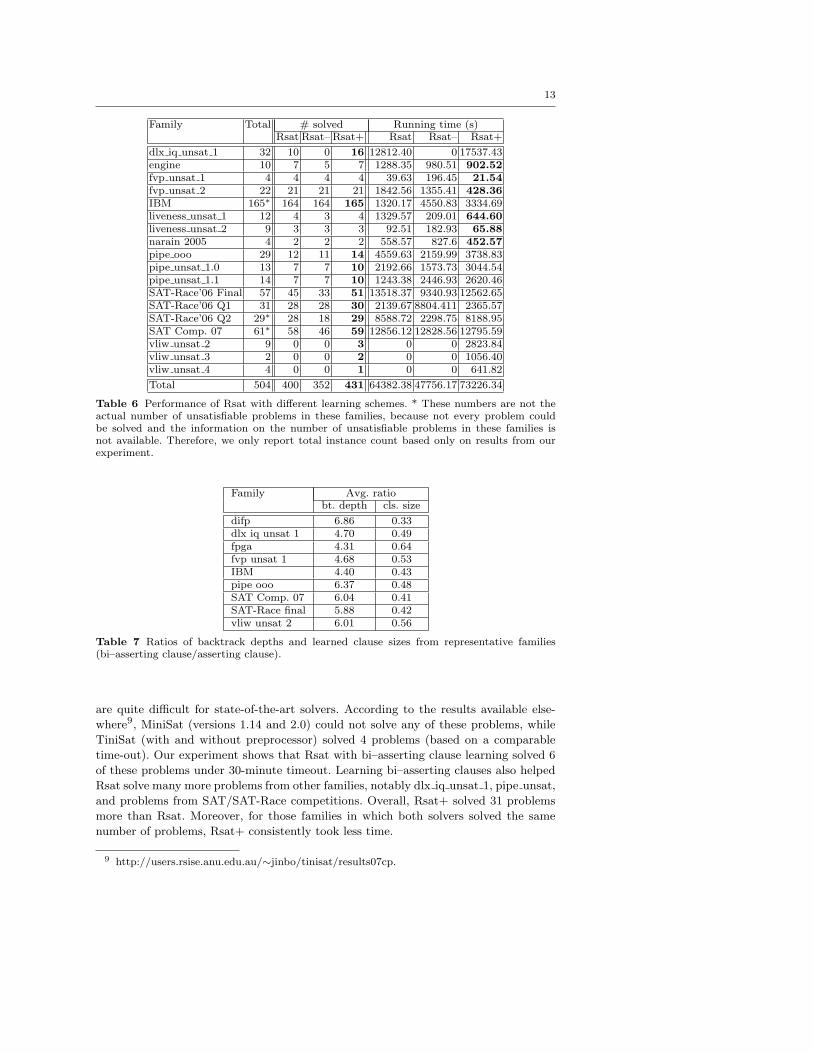
Table 6 Performance of Rsat with different learning schemes. * These numbers are not theactual number of unsatisfiable problems in these families, because not every problem couldbe solved and the information on the number of unsatisfiable problems in these families isnot available. Therefore, we only report total instance count based only on results from ourexperiment.

Family Avg. ratiobt. depth cls. size

difp 6.86 0.33dlx iq unsat 1 4.70 0.49fpga 4.31 0.64fvp unsat 1 4.68 0.53IBM 4.40 0.43pipe ooo 6.37 0.48SAT Comp. 07 6.04 0.41SAT-Race final 5.88 0.42vliw unsat 2 6.01 0.56

Table 7 Ratios of backtrack depths and learned clause sizes from representative families(bi–asserting clause/asserting clause).

are quite difficult for state-of-the-art solvers. According to the results available else-

where9, MiniSat (versions 1.14 and 2.0) could not solve any of these problems, while

TiniSat (with and without preprocessor) solved 4 problems (based on a comparable

time-out). Our experiment shows that Rsat with bi–asserting clause learning solved 6

of these problems under 30-minute timeout. Learning bi–asserting clauses also helped

Rsat solve many more problems from other families, notably dlx iq unsat 1, pipe unsat,

and problems from SAT/SAT-Race competitions. Overall, Rsat+ solved 31 problems

more than Rsat. Moreover, for those families in which both solvers solved the same

number of problems, Rsat+ consistently took less time.

9 http://users.rsise.anu.edu.au/∼jinbo/tinisat/results07cp.

14

Version Number of solved problemsSAT UNSAT Total

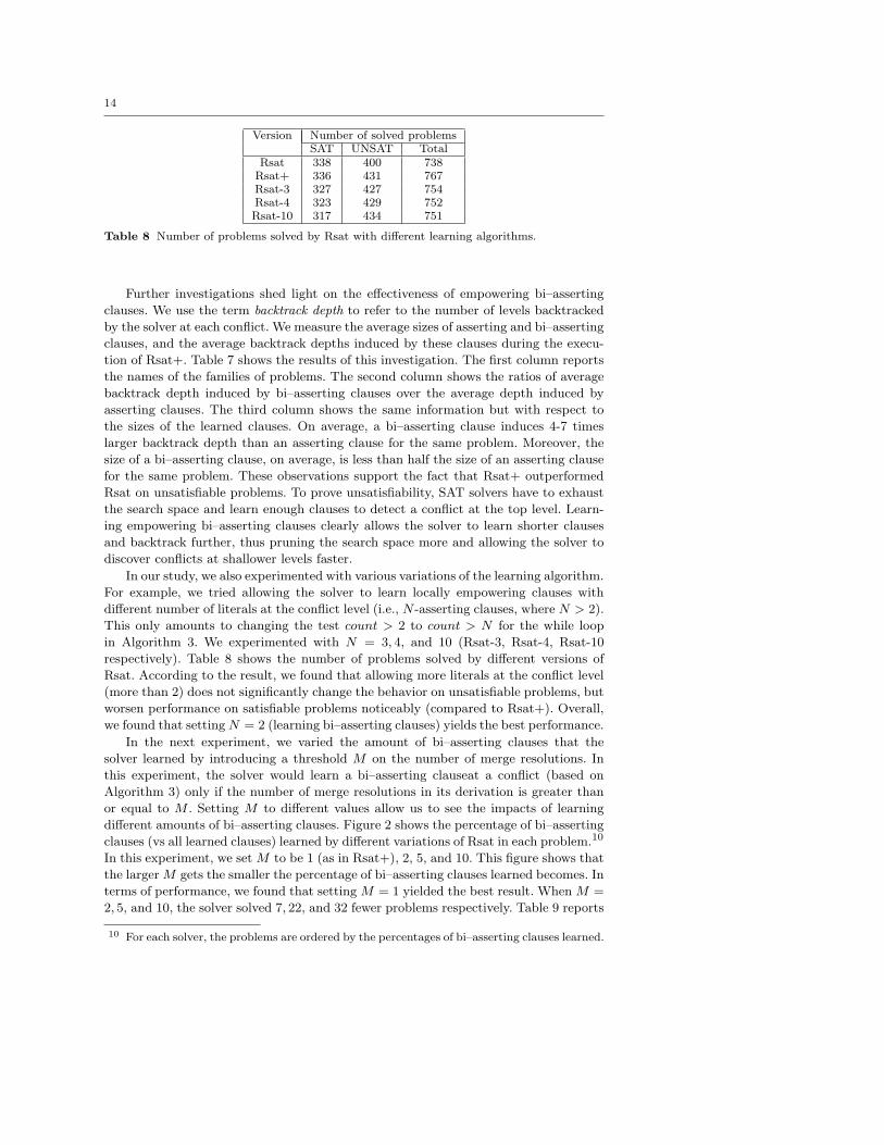
Rsat 338 400 738Rsat+ 336 431 767Rsat-3 327 427 754Rsat-4 323 429 752Rsat-10 317 434 751

Table 8 Number of problems solved by Rsat with different learning algorithms.

Further investigations shed light on the effectiveness of empowering bi–asserting

clauses. We use the term backtrack depth to refer to the number of levels backtracked

by the solver at each conflict. We measure the average sizes of asserting and bi–asserting

clauses, and the average backtrack depths induced by these clauses during the execu-

tion of Rsat+. Table 7 shows the results of this investigation. The first column reports

the names of the families of problems. The second column shows the ratios of average

backtrack depth induced by bi–asserting clauses over the average depth induced by

asserting clauses. The third column shows the same information but with respect to

the sizes of the learned clauses. On average, a bi–asserting clause induces 4-7 times

larger backtrack depth than an asserting clause for the same problem. Moreover, the

size of a bi–asserting clause, on average, is less than half the size of an asserting clause

for the same problem. These observations support the fact that Rsat+ outperformed

Rsat on unsatisfiable problems. To prove unsatisfiability, SAT solvers have to exhaust

the search space and learn enough clauses to detect a conflict at the top level. Learn-

ing empowering bi–asserting clauses clearly allows the solver to learn shorter clauses

and backtrack further, thus pruning the search space more and allowing the solver to

discover conflicts at shallower levels faster.

In our study, we also experimented with various variations of the learning algorithm.

For example, we tried allowing the solver to learn locally empowering clauses with

different number of literals at the conflict level (i.e., N -asserting clauses, where N > 2).

This only amounts to changing the test count > 2 to count > N for the while loop

in Algorithm 3. We experimented with N = 3, 4, and 10 (Rsat-3, Rsat-4, Rsat-10

respectively). Table 8 shows the number of problems solved by different versions of

Rsat. According to the result, we found that allowing more literals at the conflict level

(more than 2) does not significantly change the behavior on unsatisfiable problems, but

worsen performance on satisfiable problems noticeably (compared to Rsat+). Overall,

we found that setting N = 2 (learning bi–asserting clauses) yields the best performance.

In the next experiment, we varied the amount of bi–asserting clauses that the

solver learned by introducing a threshold M on the number of merge resolutions. In

this experiment, the solver would learn a bi–asserting clauseat a conflict (based on

Algorithm 3) only if the number of merge resolutions in its derivation is greater than

or equal to M . Setting M to different values allow us to see the impacts of learning

different amounts of bi–asserting clauses. Figure 2 shows the percentage of bi–asserting

clauses (vs all learned clauses) learned by different variations of Rsat in each problem.10

In this experiment, we set M to be 1 (as in Rsat+), 2, 5, and 10. This figure shows that

the larger M gets the smaller the percentage of bi–asserting clauses learned becomes. In

terms of performance, we found that setting M = 1 yielded the best result. When M =

2, 5, and 10, the solver solved 7, 22, and 32 fewer problems respectively. Table 9 reports

10 For each solver, the problems are ordered by the percentages of bi–asserting clauses learned.

15

0

5

10

15

20

25

30

0 100 200 300 400 500 600 700 800 900

Per

cen

tag

e o

f b

i-as

sert

ing

cla

use

s le

arn

ed

Problem number

M=1

M=2

M=5

M=10

Fig. 2 Percentages of bi-asserting clauses over all learned clauses learned by Rsat with differentmerge thresholds.

Version Number of solved problemsSAT UNSAT Total

Rsat 338 400 738Rsat+ (M = 1) 336 431 767Rsat+ (M = 2) 345 415 760Rsat+ (M = 5) 338 407 745Rsat+ (M = 10) 335 400 735

Table 9 Number of problems solved by Rsat+ with different merge thresholds.

more detailed results of this experiment. These results show that as the threshold gets

larger, fewer bi–asserting clauses are learned and the performance deteriorates. Note

that, when M = 10, the performance of the solver is quite similar to that of Rsat with

no bi–asserting clause learning in terms of the number of solved problems.

It is also interesting to note here that the percentages of bi–asserting clauses learned

by Rsat+ (M = 1) range from 5-15% on most problems. These percentages roughly

reflect the fractions of conflicts for which our learning algorithm was able to find “more

useful” learned clauses. Even though bi–asserting clauses account for a relatively small

percentage of all learned clauses, they were already able to make significant impact on

performance, especially on unsatisfiable problems.

3.5 Related Work

In [33], the authors studied various learning schemes (asserting and non-asserting) from

a graph-partitioning point of view and compared their performance empirically. Their

experimental results showed that the first UIP asserting clause learning scheme was

the most robust among the considered schemes.

Non-asserting learning schemes have also been proposed by [29], [17], and [9]. In

these papers, non-asserting clauses are learned in addition to asserting clauses (i.e.,

the solvers may learn multiple clauses for some conflicts). Moreover, additional clauses

16

. . .

0 1 2 3 k−1 k+1 k+2 k+3k

Decisionlevel

Sub-problem 1

k+4

Sub-problem 2

Erased assignmentsAssertion level

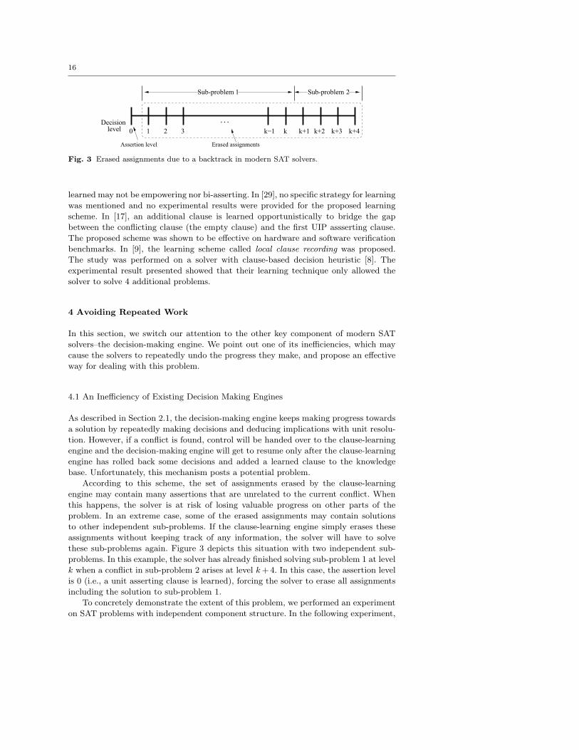
Fig. 3 Erased assignments due to a backtrack in modern SAT solvers.

learned may not be empowering nor bi-asserting. In [29], no specific strategy for learning

was mentioned and no experimental results were provided for the proposed learning

scheme. In [17], an additional clause is learned opportunistically to bridge the gap

between the conflicting clause (the empty clause) and the first UIP assserting clause.

The proposed scheme was shown to be effective on hardware and software verification

benchmarks. In [9], the learning scheme called local clause recording was proposed.

The study was performed on a solver with clause-based decision heuristic [8]. The

experimental result presented showed that their learning technique only allowed the

solver to solve 4 additional problems.

4 Avoiding Repeated Work

In this section, we switch our attention to the other key component of modern SAT

solvers–the decision-making engine. We point out one of its inefficiencies, which may

cause the solvers to repeatedly undo the progress they make, and propose an effective

way for dealing with this problem.

4.1 An Inefficiency of Existing Decision Making Engines

As described in Section 2.1, the decision-making engine keeps making progress towards

a solution by repeatedly making decisions and deducing implications with unit resolu-

tion. However, if a conflict is found, control will be handed over to the clause-learning

engine and the decision-making engine will get to resume only after the clause-learning

engine has rolled back some decisions and added a learned clause to the knowledge

base. Unfortunately, this mechanism posts a potential problem.

According to this scheme, the set of assignments erased by the clause-learning

engine may contain many assertions that are unrelated to the current conflict. When

this happens, the solver is at risk of losing valuable progress on other parts of the

problem. In an extreme case, some of the erased assignments may contain solutions

to other independent sub-problems. If the clause-learning engine simply erases these

assignments without keeping track of any information, the solver will have to solve

these sub-problems again. Figure 3 depicts this situation with two independent sub-

problems. In this example, the solver has already finished solving sub-problem 1 at level

k when a conflict in sub-problem 2 arises at level k +4. In this case, the assertion level

is 0 (i.e., a unit asserting clause is learned), forcing the solver to erase all assignments

including the solution to sub-problem 1.

To concretely demonstrate the extent of this problem, we performed an experiment

on SAT problems with independent component structure. In the following experiment,

17

Average running time (s)Instance Name MiniSat MiniSat with prog. sv.

Original Replicated Ratio Original Replicated Ratio

difp 19 0 arr rcr 33.78 1,288.09 38.13 24.57 155.75 6.34difp 19 1 arr rcr 22.41 1,359.74 60.68 33.84 221.21 6.54IBM FV 2004 1 02 3.k70 6.66 658.96 98.96 0.85 12.88 15.23IBM 19 rule SAT dat.k30 3.77 125.20 33.24 2.09 22.77 10.89IBM 21 rule SAT dat.k35 8.06 617.30 76.58 2.82 28.01 9.93vange-color-inc-54 12.58 1,661.98 132.12 2.64 55.02 20.87vmpc 21.renamed-sat05-1923 8.24 354.06 42.96 2.42 32.41 13.41vmpc 21.shuffled-sat05-1955 5.87 230.59 39.29 2.94 19.94 6.79vmpc 23.renamed-sat05-1927 179.34 1,720.27 9.59 6.95 64.01 9.20

Table 10 Average running time (in seconds) of MiniSat with and without progress saving.The ratio columns show the ratios of average running time on replicated instances over thaton original instances.

we artificially generated SAT problems that would cause work repetition in conven-

tional clause-learning SAT solvers. Each problem was generated by concatenating four

identical copies of a satisfiable problem. These bigger problems will be referred to as

replicated problems throughout this paper.

Table 10 reports the results of this initial experiment, conducted using MiniSat [10],

on a computer with a 3.8GHz processor and 2GB of RAM. For each problem, we ran

each version of MiniSat 10 times with random initial variable orderings.11 The first

column of the table shows the name of the problems used and the next 2 columns

reports the average running time of MiniSat on each original and replicated problem.

The forth column shows the ratio of the average running time on replicated problem

to that on the corresponding original problem. As the result shows, solving a repli-

cated problem can be more than two orders of magnitudes less efficient, even though

a replicated problem contains four identical copies of the original problem.

0

200

400

600

800

1000

1200

1400

1600

1800

0 50000 100000 150000 200000 250000 300000 350000 400000 450000

Vari

ab

le i

nd

ex

Decision number

0

200

400

600

800

1000

1200

1400

1600

1800

0 50000 100000 150000 200000 250000 300000

Vari

able

index

Decision number

Fig. 4 Decision behavior on a replicated instance of MiniSat (left) and MiniSat with progresssaving (right). Both x-axes represent the chronological order of decisions.

Further investigation on these problems reveals the source of inefficiency. In Fig-

ure 4, we plot the indices of decision variables set by MiniSat in chronological order. The

11 We set the timeout of each run to 1,800 seconds. Any run with longer running timecontributed 1,800 seconds in the computation of average running time.

18

left plot in Figure 4 shows such a plot based on one run of MiniSat on the replicated in-

stance of vmpc 21.shuffled-sat05-1955. Variable indices in the replicated instance range

from 1 to 1764 (4× 441 original variables). Each component in the instance occupies a

contiguous range of variable indices. Each dark band in this plot indicates the solver’s

attempt to solve a component.12 We can see in the left plot of Figure 4 that MiniSat

ended up solving all components multiple times. Most of the attempts to re-solve a

component take non-trivial amount of work, as illustrated by the width of each band.

This clearly illustrates that work repetition is responsible for a fair amount of the

disproportionate increase in runtime of the solver on the replicated instances.

4.2 Progress Saving

To deal with the problem of work repetition, in [26], we proposed to deal with this prob-

lem with a lightweight component caching technique called progress saving. Progress

saving is a simple way of preventing the decision-making engine from having to solve

the same sub-problem multiple times. To achieve this, we only need to record the value

of every variable assignment that the clause-learning engine erases. This information

should then be made available to the decision-making engine. In the future, whenever

the decision-making engine decides to make a decision on a variable, it should assign

the recorded value to that variable. If the variable chosen for making decision was

never assigned a value before, the decision-making engine should proceed with the de-

fault heuristic. Note that, according to this algorithm, both decisions and implications

should be saved whenever the solvers backtrack. The time and space overhead of this

technique is only linear in the number of variables.

In practice, independent sub-problems may exist as parts of the original problem

structure or may be created/destroyed dynamically as assignments are made/erased

by the solver. A nice property of the proposed technique is that once an independent

sub-problem has been solved, each future attempt to solve the sub-problem will require

time that is only linear in the size of the sub-problem (without progress saving, this

becomes exponential in the worst case). This property holds for the independent sub-

problem as long as it is not destroyed.13

We evaluated the proposed solution on the replicated problems from the previous

experiment. The result of this experiment is shown in the last 3 columns of Table 10.

Clearly, progress saving improves the running time of MiniSat by up to an order of mag-

nitude on these problems. The ratios of running time on replicated problems over that

on original problems also decrease considerably. In fact, for several of these problems,

the ratios are only slightly greater than the number of identical copies (4). Further-

more, the right plot of Figure 4 shows the behavior of MiniSat with progress saving on

the replicated problem of vmpc 21.shuffled-sat05-1955. In this case, each sub-problem

is “solved” only once (one dark band at any horizontal level). Note that, in the right

plot, each sub-problem is still visited more than once as expected. However, each visit

after the first attempt on the sub-problem requires little effort from the solver. These

later visits correspond to the scattered groups of points after each dark band.

12 Our investigation revealed that, in most cases, MiniSat only switched sub-problems whenit had finished solving a sub-problem.13 A sub-problem that is created by variable assignments can be destroyed when some of

those assignments are erased.

19

vmpc 23.renamed-as.sat05-1927 difp 19 0 wal rcr

0 2 4 6 8 100

1

2

3

4

5

6x 10

4

Number of independent components

Ru

nn

ing

tim

e (s

)

MiniSatMiniSat with prog. sv.Linear running time

0 2 4 6 8 100

1

2

3

4

5

6x 10

4

Number of independent components

Ru

nn

ing

tim

e (s

)

MiniSatMiniSat with prog. svLinear running time

ibm 19 rule SAT dat.k30 bmc-ibm-10

0 2 4 6 8 100

500

1000

1500

2000

Number of independent components

Ru

nn

ing

tim

e (s

)

MiniSatMiniSat with prog. sv.Linear running time

0 5 10 150

200

400

600

800

1000

Number of independent components

Runnin

g t

ime

(s)

MiniSatMiniSat with prog. sv.Linear running time

Fig. 5 Running time of MiniSat on replicated instances with varied number of components.Hypothetical linear (on the number of components) running time is also depicted in each plot.

Next, we compare the scalability of MiniSat with and without progress saving. The

results are shown in Figure 5. In this experiment, we tested both versions of the solver

on problems with varied number of independent sub-problems. The x-axis of each plot

in this figure indicates the number of sub-problems presented in the problem, while

the y-axis corresponds to the running time of the solver. In each plot, we show the

running time of both solvers together with the hypothetical linear running time on

the problems. According to these plots, the running time of MiniSat without progress

saving increases rapidly as the number of sub-problems increases, whereas the running

time of MiniSat with progress saving appears to be only slightly worse than linear in

the number of sub-problems.

4.3 Evaluation on Real-World Problems

We will now present results of evaluating the proposed technique on real-world SAT

problems. Most of these problems do not decompose into multiple sub-problems ini-

tially. However, after setting some variables, some problems may eventually decompose.

20

In [6], the authors demonstrated the prevalence of independent sub-problem structure

in real-world instances.

We used 1,403 industrial problems from the SAT competitions and from contem-

porary benchmark libraries.14 All experiments were performed on a machine with a

3.8 GHz CPU and 2GB of RAM, with a time-out limit of 1800 seconds. We considered

several versions of MiniSat in this experiment. By default, MiniSat 1.14 always sets

the decision variables to false. To demonstrate the effectiveness of progress saving, we

also considered two natural modifications to MiniSat’s decision-making engine; setting

the decision variables to true and setting them to values drawn randomly at decision

time.

0

200

400

600

800

1000

1200

1400

1600

1800

450 500 550 600 650 700

Runnin

g t

ime

(s)

Number of instances solved

MiniSatMiniSat [positive]MiniSat [random]

MiniSat+pg. sv.

0

200

400

600

800

1000

1200

1400

1600

1800

450 500 550 600 650 700

Runnin

g t

ime

(s)

Number of instances solved

MiniSatMiniSat [positive]MiniSat [random]

MiniSat+pg. sv.

Fig. 6 Running time profiles of three variations of MiniSat and of MiniSat with progresssaving. The left plot shows profiles on satisfiable problems while the right plot shows those onunsatisfiable problems.

Figure 6 shows the running time profiles of the considered versions of MiniSat

on satisfiable and unsatisfiable problems. First of all, these plots show that simply

changing the phase selection heuristic to always set variables positively or randomly

does not significantly effect performance either on satisfiable or unsatisfiable problems.

However, it is clear that MiniSat with progress saving stands out from other variations

on satisfiable problems. It solved 49, 32, and 63 more satisfiable problems than Min-

iSat, MiniSat [positive], and MiniSat [random], respectively. The right plot of Figure 6

shows that all versions of MiniSat considered essentially have the same performance

on unsatisfiable problems. This result demonstrates that even in the cases where there

are no solutions to be saved, progress saving does not impair the performance of the

solver.

Progress saving was first used in the context of SAT in Rsat [25] in SAT-Race

2006.15 Since then, it has been adopted by many other top SAT solvers including

MiniSat [30], PicoSat [5], TiniSat [16], and ManySat [32].

14 http://www.satcompetition.org ,http://www.research.ibm.com/haifa/projects/verification/RB Homepage/fvbenchmarks.html,http://miroslav-velev.com/sat benchmarks.html.15 For more information, see the SAT-Race 2006 website at http://fmv.jku.at/sat-race-2006/.

21

4.4 Related Work

The problem of non–chronological backtracking erasing progress made by the decision-

making engine has long been observed in the context of CSP. In [13], the author pro-

posed dynamic backtracking as a solution to this problem. This technique allows the

solver to specifically undo a bad assignment instead of backtracking to it. This approach

is superficially similar to ours. However, it may cause the problem to become overly-

constrained after backtracking, as pointed out by the author. Moreover, implementing

this approach in the contemporary SAT framework would require a careful modification

to make it work as intended. Neither is the case for our proposed technique.

Frost and Dechter have also experimented with this idea in CSP. In [12], a heuristic

called sticking value was used in a CSP solver without any learning and was evaluated

only on randomly generated CSP problems. Their experimental results showed that,

in the considered settings, this heuristic reduced the running time by a factor of two

on a few problems with small-sized variable domains.

In [6], Biere and Sinz showed that independent components do exist in some real-

world SAT instances and proposed a method to take advantage of the structure. How-

ever, their approach is semi–dynamic, as it only considers permanent decompositions

that occur in the absence of any decision and requires a component detection algo-

rithm, which could incur a high overhead. Although experimental results on artificially

generated instances shows improvements, no gain was reported on industrial bench-

marks.

5 Conclusions

We presented a simple model of modern SAT solvers that highlights the roles of the

two main components in these solvers: the decision-making engine and the clause-

learning engine. Then, based on our model, we discussed two limitations of modern

SAT solvers and proposed two techniques for dealing with them. One technique is a

new clause-learning scheme that allows the solvers to consider a broader set of learned

clauses while maintaining empowerment. The other is a phase selection heuristic that

serves as a partial caching mechanism, which reduces a negative effect of the clause-

learning engine on the decision-making engine of modern SAT solvers. We demonstrated

through experimental results that both proposed techniques significantly improved the

performance of the considered solvers.

A Proofs

This section is entirely dedicated to formalizing and proving the claim made in Section 3.3.The claim itself is formalized in Proposition 1. This proposition is then proved through a seriesof lemmas (Lemmas 1,2,3).

Before we can state the proposition, we first formalize the type of resolution performed byAlgorithm 2.

Definition 1 A resolution derivation of the clause Ck from the CNF ∆ is a sequence of clausesΠ = C1, C2, ..., Ck where each clause Ci is either in ∆ or is a resolvent of clauses precedingCi. Furthermore,

– Π is linear if each clause Ci for i ≥ 3 is either in ∆ or is the resolvent of Ci−2 and Ci−1.The clauses C1, C2, C4, C6, C8, . . . of a linear resolution are called the non-resolvents ofthe derivation.

22

– Π is causal if it is linear and if the resolved variable x of Ci and Ci+1 does not appear inclauses Ci+2, . . . , Ck.

We now formalize the claim using the above definition.

Proposition 1 Let Π be a causal resolution derivation of the clause C. C is empoweringwith respect to the non-resolvents in Π if Π contains a merge resolution step.

We will prove this proposition with a series of lemmas. The proof makes extensive use ofthe fact that for a conjunction of literals σ and CNF ∆, we have ∆∧σ = (∆|σ)∧σ. Here, ∆|σis the CNF obtained by removing any clause in ∆ that mentions any literal in σ and removingany literal from ∆ whose negation appears in σ. Hence, none of the variables in σ will appearin ∆|σ. The following formal definition of empowerment is needed in the proofs.

Definition 2 (Empowerment [28]) Let α ⇒ ` be a clause where ` is a literal and α is aconjunction of literals. The clause is empowering with respect to CNF ∆ via ` iff

1. ∆ |= (α ⇒ `): the clause is implied by ∆.2. ∆ ∧ α 6` `: the literal ` cannot be derived from ∆ ∧ α using unit resolution.

The following lemma gives the basis for generating empowering clauses.

Lemma 1 (Generation of Empowerment) If C3 is the resolvent of a merge resolutionbetween C1 = (x∨ `∨α) and C2 = (¬x∨ `∨β), then C3 is empowering with respect to C1∧C2

and ` is its empowering literal.

Proof Let σ = ¬(α ∨ β). Clearly, C3 = σ ⇒ `. Consider C1 ∧ C2 ∧ σ = (C1 ∧ C2)|σ ∧ σ =(`∨x)∧(`∨¬x)∧σ. Clearly, unit resolution cannot derive ` from this. Hence, C3 is empoweringwith respect to C1 ∧ C2 and ` is an empowering literal. utLemma 2 (Backward Preservation of Empowerment) Let C1, C2, . . . , Ck be a causalresolution. If Ck is empowering with respect to {C3, . . . , Ck−1}, then Ck is also empoweringwith respect to {C1, . . . , Ck−1}.

This lemma holds because C3, the resolvent of C1, C2, is essentially ∃x(C1 ∧C2), where xis the resolved variable. Hence, adding C1, C2 to the formula that already contains C3 cannotgive us any new knowledge other than that on the resolved variable, which does not appearelsewhere in the derivation (because it is causal). Therefore, Ck must still be empowering withrespect to the new knowledge base.

The combination of the above lemmas show that the final product of a causal resolutionderivation whose last step is a merge resolution is always empowering with respect to thenon-resolvents of the derivation. The next lemma shows that once an empowering clause isobtained from a causal derivation, all further derived clauses will also be empowering.

If Π = C1, ..., Cn is a linear resolution derivation, we will use NR(Π) to denote thenon-resolvents of Π (i.e., NR(Π) = {C1} ∪ {Ci|2 ≤ i ≤ n, i is even}).Lemma 3 (Forward Preservation of Empowerment) Let Π? = C1, ..., Cn and Π =Π?, Cn+1, Cn+2, where Cn+2 = C, be causal resolution derivations from clauses in ∆. If Cn

is empowering with respect to NR(Π?), then C is empowering with respect to NR(Π).

Proof Clearly, NR(Π) = NR(Π?) ∧ Cn+1. Let x be the resolved variable of Cn and Cn+1.We may assume that Cn and Cn+1 do not share a literal.16 With this assumption, we havethat

Cn+1 and the clauses of NR(Π?) cannot share any variable other than x. (1)

Otherwise, any common variable between Cn+1 and NR(Π?) must remain unresolved in Π?

(because Π is causal, which does not allow any resolved variable to reappear) and must there-fore appear in Cn, which would contradiction our assumption that Cn and Cn+1 share nocommon literal. Let ` be the empowering literal of Cn (with respect to NR(Π?)). Because Cn

is empowering, we have

NR(Π?) ∧ ¬(Cn\{`}) 6` `. (2)

There are two cases to consider:

16 Otherwise, C, is empowering with respect to NR(Π) by the results in Lemmas 1,2.

23

1. ` 6= x. Assume, WLOG, that Cn = (x ∨ ` ∨ α) and Cn+1 = (¬x ∨ β). We then haveC = (¬α ∧ ¬β) ⇒ `. Consider NR(Π) ∧ ¬α ∧ ¬β = NR(Π?) ∧ Cn+1 ∧ ¬α ∧ ¬β. In thiscase, Cn+1 can only generate ¬x as an implication. However, this will not allow NR(Π?) toproduce `, because we know from (2) that NR(Π?)∧¬α∧¬x 6` `. Since, from (1), NR(Π?)does not mention any variable in β, we can safely conclude that NR(Π) ∧ ¬α ∧ ¬β 0 `.

2. ` = x or ` = ¬x. Assume, WLOG, Cn = `∨α and Cn+1 = ¬`∨β. Let y be any literal in βand σ = ¬(C\{y}). Clearly, C = σ ⇒ y. Now, consider NR(Π)∧σ = NR(Π?)∧Cn+1∧σ.The literal y only appears in Cn+1 which becomes (¬`∨y) under σ. However, NR(Π?)∧σcannot produce `, which is needed by Cn+1 to imply y, because we know that, from (1),NR(Π?) does not mention any variable in β, and that, from (2), NR(Π?) ∧ ¬α 6` `.Therefore, NR(Π) ∧ σ 0 `.

Hence, C is empowering wrt NR(Π) in both cases. ut

Together, these lemmas prove the result in Proposition 1.

References

1. Andrews, P. B. Resolution with merging. J. ACM 15, 3 (1968), 367–381.2. Audemard, G., Bordeaux, L., Hamadi, Y., Jabbour, S., and Sais, L. A generalized

framework for conflict analysis. In SAT (2008), pp. 21–27.3. Bacchus, F., and Winter, J. Effective preprocessing with hyper-resolution and equality

reduction. In In SAT (2003), pp. 341–355.4. Beame, P., Kautz, H., and Sabharwal, A. Towards understanding and harnessing the

potential of clause learning. JAIR 22 (2004), 319–351.5. Biere, A. Picosat essentials. Journal on Satisfiability, Boolean Modeling and Computation

(JSAT) (2008), 75–97.6. Biere, A., and Sinz, C. Decomposing sat problems into connected components. Journal

on Satisfiability, Boolean Modeling and Computation (JSAT) 2 (2006).7. Davis, M., Logemann, G., and Loveland, D. A machine program for theorem-proving.

Commun. ACM 5, 7 (1962), 394–397.8. Dershowitz, N., Hanna, Z., and Nadel, A. A clause-based heuristic for sat solvers. In

Proceedings of 8th International Conference on Theory and Applications of SatisfiabilityTesting(SAT) (2005), pp. 46–60.

9. Dershowitz, N., Hanna, Z., and Nadel, A. Towards a better understanding of thefunctionality of a conflict-driven sat solver. In SAT (2007), pp. 287–293.

10. Een, N., and Sorensson, N. An extensible sat-solver. In SAT (2003), pp. 502–518.11. En, N., and Biere, A. Effective preprocessing in sat through variable and clause elimi-

nation. In In proc. SAT05, volume 3569 of LNCS (2005), Springer, pp. 61–75.12. Frost, D., and Dechter, R. In search of the best constraint satisfaction search. In AAAI

’94: Proceedings of the twelfth national conference on Artificial intelligence (vol. 1) (MenloPark, CA, USA, 1994), American Association for Artificial Intelligence, pp. 301–306.

13. Ginsberg, M. L. Dynamic backtracking. Journal of Artificial Intelligence Research 1(1993), 25–46.

14. Goldberg, E., and Novikov, Y. Verification of proofs of unsatisfiability for cnf formulas.In Proceedings of DATE2003 (2003).

15. Hertel, P., Bacchus, F., Pitassi, T., and Van Gelder, A. Clause learning can effec-tively p-simulate general propositional resolution. In Proc. of AAAI-08 (2008), pp. 283–290.

16. Huang, J. A case for simple sat solvers. In CP-07 (2007), pp. 839–846.17. Jin, H., and Somenzi, F. Strong conflict analysis for propositional satisfiability. In DATE

’06: Proceedings of the conference on Design, automation and test in Europe (3001 Leuven,Belgium, Belgium, 2006), European Design and Automation Association, pp. 818–823.

18. Le Berre, D. Exploiting the real power of unit propagation lookahead. In Workshopon Theory and Applications of Satisfiability Testing(SAT’01) (Boston University, Mas-sachusetts, USA, June 2001), H. Kautz and B. Selman, Eds., Elsevier Science Publishers,pp. 59–80.

19. Li, C. M. Heuristics based on unit propagation for satisfiability problems. In Proceedingsof IJCAI-97 (1997), pp. 366–371.

24

20. Li, C. M. A constraint-based approach to narrow search trees for satisfiability. Inf.Process. Lett. 71, 2 (1999), 75–80.

21. Lynce, I., and Marques-Silva, Jo a. Probing-based preprocessing techniques for propo-sitional satisfiability. In ICTAI ’03: Proceedings of the 15th IEEE International Confer-ence on Tools with Artificial Intelligence (Washington, DC, USA, 2003), IEEE ComputerSociety, p. 105.

22. Marques-Silva, J. P., and Sakallah, K. A. GRASP - A New Search Algorithm forSatisfiability. In Proceedings of IEEE/ACM International Conference on Computer-AidedDesign (1996), pp. 220–227.

23. Moskewicz, M., Madigan, C., Zhao, Y., Zhang, L., and Malik, S. Chaff: Engineeringan efficient sat solver. pp. 530–535.

24. Nieuwenhuis, R., Oliveras, A., and Tinelli, C. Solving sat and sat modulo theories:From an abstract davis–putnam–logemann–loveland procedure to DPLL(T). Journal ofACM 53, 6 (2006), 937–977.

25. Pipatsrisawat, K., and Darwiche, A. Rsat 1.03: Sat solver description. Tech. Rep.D–152, Automated Reasoning Group, Computer Science Department, UCLA, 2006.

26. Pipatsrisawat, K., and Darwiche, A. A lightweight component caching scheme forsatisfiability solvers. In Proceedings of 10th International Conference on Theory andApplications of Satisfiability Testing(SAT) (2007), pp. 294–299.

27. Pipatsrisawat, K., and Darwiche, A. Rsat 2.0: Sat solver description. Tech. Rep. D–153,Automated Reasoning Group, Comp. Sci. Department, UCLA, 2007.

28. Pipatsrisawat, K., and Darwiche, A. A new clause learning scheme for efficient un-satisfiability proofs. In Proceedings of the Twenty-Third AAAI Conference on ArtificialIntelligence (AAAI) (2008), pp. 1481–1484.

29. Ryan, L. Efficient Algorithms for Clause-Learning SAT Solvers. Master’s thesis, SimonFraser University, 2004.

30. Sorensson, N., and Een, N. Minisat 2.1 and minisat++ 1.0–sat race 2008 editions, 2008.31. Subbarayan, S., , Subbarayan, S., and Pradhan, D. K. Niver: Non increasing vari-

able elimination resolution for preprocessing sat instances. In In Proc. 7th InternationalConference on Theory and Applications of Satisfiability Testing (SAT (2004), Springer,pp. 276–291.

32. Youssef Hamadi, S. J., and Sais, L. Manysat: solver description. Tech. Rep. MSR-TR-2008-83, 2008.

33. Zhang, L., Madigan, C. F., Moskewicz, M. W., and Malik, S. Efficient conflict drivenlearning in boolean satisfiability solver. In ICCAD (2001), pp. 279–285.