J. Math. Anal. Appl. 354 (2009) 347–359

Contents lists available at ScienceDirect

Journal of Mathematical Analysis and Applications

www.elsevier.com/locate/jmaa

A systematization of the saddle point method.Application to the Airy and Hankel functions

José L. López ∗, Pedro Pagola, Ester Pérez Sinusía

Departamento de Ingeniería Matemática e Informática, Universidad Pública de Navarra, 31006 Pamplona, Spain

a r t i c l e i n f o a b s t r a c t

Article history:Received 2 October 2008Available online 24 December 2008Submitted by M. Milman

Keywords:Asymptotic expansions of integralsSaddle point methodAiry functionHankel function

The standard saddle point method of asymptotic expansions of integrals requires to showthe existence of the steepest descent paths of the phase function and the computation ofthe coefficients of the expansion from a function implicitly defined by solving an inversionproblem. This means that the method is not systematic because the steepest descent pathsdepend on the phase function on hand and there is not a general and explicit formula forthe coefficients of the expansion (like in Watson’s Lemma for example). We propose a moresystematic variant of the method in which the computation of the steepest descent pathsis trivial and almost universal: it only depends on the location and the order of the saddlepoints of the phase function. Moreover, this variant of the method generates an asymptoticexpansion given in terms of a generalized (and universal) asymptotic sequence that avoidsthe computation of the standard coefficients, giving an explicit and systematic formulafor the expansion that may be easily implemented on a symbolic manipulation program.As an illustrative example, the well-known asymptotic expansion of the Airy function isrederived almost trivially using this method. New asymptotic expansions of the Hankelfunction Hn(z) for large n and z are given as non-trivial examples.

© 2008 Elsevier Inc. All rights reserved.

1. Introduction

Consider integrals of the form

F (x) :=∫C

exf (z) g(z)dz, (1)

where C is a bounded or unbounded path in the complex plane, x is a large positive parameter and f (z) and g(z) areanalytic functions in a domain of the complex plane containing the path C . The standard saddle point method tells us thatthe major contribution to the integral (1) comes from the neighborhoods of the relevant saddle points of f (z) [8, Chapter 2,Section 4]. For instance, suppose that f (z) has only one saddle point z0 ∈ C of multiplicity one ( f ′(z) = 0 and f ′′(z) �= 0)and that we can deform the path C to a steepest descent path Γ̃ through z0:

F (x) =∫Γ̃

exf (z) g(z)dz. (2)

* Corresponding author.E-mail addresses: jl.lopez@unavarra.es (J.L. López), pedro.pagola@unavarra.es (P. Pagola), ester.perez@unavarra.es (E.P. Sinusía).

0022-247X/$ – see front matter © 2008 Elsevier Inc. All rights reserved.doi:10.1016/j.jmaa.2008.12.032

348 J.L. López et al. / J. Math. Anal. Appl. 354 (2009) 347–359

Then, applying the saddle point method we have:

F (x) ∼ g(z0)

√2π

− f ′′(z0)xexf (z0), x → ∞. (3)

The right-hand side above is the first term of a complete asymptotic expansion that can be obtained following the standardsaddle point procedure explained in [8, Chapter 2, Section 4] for example. That method has two main technical difficulties:

(i) to compute or at least show the existence of the steepest descent paths of f (z), and(ii) the inversion problem originated by a change of variables (see details in Section 2 of this paper).

(For example, in [6, Chapter 4, Section 7] only an explicit formula for the two first coefficients of the expansion is given.In [8, Chapter 2, Section 4], the first terms of an asymptotic expansion of the Hankel function are derived, but an explicitalgorithm for the computation of the whole expansion is not given.) Because of these two technical difficulties, the standardmethod is not a systematic method: for every concrete integral F (x) on hand, we have to show the existence of appropriatesteepest descent paths of f (z) and solve an inversion problem to compute the coefficients of the expansion.

We can find in the literature methods and more or less explicit formulas that simplify the computation of the coefficientsof the expansion ([1, Eq. (8)], [2,4,7] [8, Chapter 2, Section 5]), avoiding the inversion problem. In another direction, it issuggested in [5] that the computation of the steepest descent path is not necessary, but only the location of the valleysof the phase function. Following the ideas suggested in some of those references, we propose here a different way tosimplify and systematize the saddle point method which avoids non-trivial steepest descent paths and change of variables.On the one hand, with this method, the steepest descent paths are trivial and universal: straights. On the other hand, thecomputation of the standard coefficients is not required because the asymptotic expansion is given in terms of a differentgeneralized asymptotic sequence. In this way, we obtain a universal and explicit form for a new asymptotic expansion ofF (x) that may be easily implemented on a symbolic manipulation program. This is shown in Section 2. In Section 3 weapply the idea to some special functions like the Airy and Hankel functions. Section 4 contains some final remarks.

2. The modified saddle point method

As in the standard saddle point method, we consider only the relevant saddle points z0 of the phase function f (z):f ′(z0) = 0 and ( f (z0)) is maximal. Assume also that the number of relevant saddle points z0 is finite and they areisolated saddle points (we do not consider here coalescing saddle points and uniformity aspects). In the standard saddlepoint method, the path C must be deformed to a new steepest descent path Γ̃ running through all of the relevant saddlepoints. By subdividing the path Γ̃ if necessary, we may assume that f (z) has only one relevant saddle point z0 on Γ̃ . If z0is a saddle point of order m − 1 with m � 2, then f ′(z0) = f ′′(z0) = · · · = f (m−1)(z0) = 0 and f (m)(z0) = aeiφ �= 0, with a > 0and 0 � φ < 2π . Inspired on the idea of Burkhardt and Perron [3, Chapter 2], we write the phase function f (z) in the form:

f (z) = fm(z) + f p(z),

with

fm(z) := f (z0) + f (m)(z0)

m! (z − z0)m

and

f p(z) := f (z) − fm(z) = f (p)(z0)

p! (z − z0)p + f (p+1)(z0)

(p + 1)! (z − z0)p+1 + · · · .

The integer m is the degree of the first non-vanishing derivative of f (z) at z = z0 and the integer p is the degree of thenext non-vanishing derivative.

The first difficulty in the standard saddle point method consists of finding the m steepest descent paths Γ̃k , k =0,1, . . . ,m − 1, of f (z) emanating from the saddle point z0: those paths in the complex plane satisfying ( f (z)) = ( f (z0))

and z0 is a maximum of ( f (z)) through Γ̃k . We propose the following modification of the method. Instead of consideringthe steepest descent paths Γ̃k of the complete phase function f (z), consider the steepest descent paths Γk of the functionfm(z): those paths in the complex plane satisfying ( fm(z)) = ( fm(z0)) = 0 and z0 is a maximum of ( f (z)) through Γk .Of course, the point z0 is a saddle point of both functions f (z) and fm(z), but, whereas the m steepest descent paths Γ̃k off (z) emanating from z0 may be hard to compute, the m steepest descent paths Γk of fm(z) are very simple: m semi-infinitestraight lines departing from z0 (see Fig. 1),

Γk :={

z ∈ C, z = z0 + reiθk , θk = (2k + 1)π − φ

m, r � 0

}, k = 0,1,2, . . . ,m − 1. (4)

Observe that ( f p(z)) = O(z − z0)p−m × ( fm(z) − f (z0)) when z → z0 and then, the steepest descent straights of fm(z)

are tangent to the steepest descent paths of f (z) at z = z0 (see Fig. 1).

J.L. López et al. / J. Math. Anal. Appl. 354 (2009) 347–359 349

Fig. 1. Typical portrait of the steepest descent paths of f (z) and fm(z) emanating from the saddle point z0 with m = 3 and φ = 0. Continuous thick linesrepresent the three steepest descent paths Γn , n = 0,1,2, of f3(z), whereas the thick dashed lines represent the three steepest descent paths Γ̃n , n = 0,1,2of f (z). They are tangent at z0.

Fig. 2. Typical portrait of the different paths considered in the text at the saddle point z0 of a phase function f (z) with m = 2 (N = 0 and M = 1): theoriginal path C , the steepest descent path Γ̃ = Γ̃0 ∪ Γ̃1 of the function f (z), the steepest descent path Γ0 ∪Γ1 of the function f2(z) and the new integrationpath Γ = Γz0 ∪ Γε . The path Γz0 ⊂ Γ0 ∪ Γ1 is contained in the disk D R (z0).

In the standard saddle point method we deform C to a steepest descent path of f (z): Γ̃ = Γ̃N ∪ Γ̃M for appropriate0 � N , M < m. We propose here a different deformation. Cut the semi-infinite straight lines ΓN and ΓM at the pointsz0 + RN eiθN and z0 + RM eiθM respectively and join the finite portions obtained after the cut (see Fig. 2):

Γz0 := {z ∈ C, z = z0 + reiθN , 0 � r � RN

} ∪ {z ∈ C, z = z0 + reiθM , 0 � r � RM

}= [

z0, z0 + RN eiθN] ∪ [

z0, z0 + RM eiθM].

We require for Γz0 to be contained inside the disk of convergence D R(z0) of the Taylor series of f (z) and g(z) at z = z0,that is, 0 < RN , RM < R (see Fig. 2).

Consider the deformation C → Γ , with Γ := Γz0 ∪ Γε and Γε is a path which joins Γz0 at its extreme points z0 + RN eiθN

and z0 + RM eiθM (see Fig. 2). We must choose the path Γε in such a way that:

(i) we can deform C → Γ (like in the standard saddle point method), and(ii) the contribution of Γε to the integral F (x),

∫Γε

exf (z) g(z)dz, is negligible (exponentially small) compared with the con-

tribution of Γz0 ,∫Γz0

exf (z) g(z)dz.

Then, whereas in the standard saddle point method we are led to

F (x) =∫C

exf (z) g(z)dz =∫Γ̃

exf (z) g(z)dz,

we propose here:

350 J.L. López et al. / J. Math. Anal. Appl. 354 (2009) 347–359

F (x) =∫C

exf (z) g(z)dz =∫Γ

exf (z) g(z)dz ∼∫

Γz0

exf (z) g(z)dz.

Once we have deformed C → Γ̃ , the next step in the standard saddle point method consists of a change of variable z → tover every one of the two steepest descent paths Γ̃N , and Γ̃M : t = f (z0) − f (z), which implicitly defines z(t) over everyone of the two paths Γ̃N , and Γ̃M . Because ( f (z)) = ( f (z0)) for z ∈ Γ̃N and z ∈ Γ̃M and z0 is a maximum of ( f (z)), wehave that the new variable t is positive over the paths Γ̃N and Γ̃M emanating from z0. Then, in the standard saddle pointmethod:

F (x) =∫Γ

exf (z) g(z)dz ∼ exf (z0)

[ ∞∫0

e−xthN (t)dt +∞∫

0

e−xthM(t)dt

], (5)

with

hN(t) := g(z(t)

)dz

dt, z ∈ Γ̃N and hM(t) := g

(z(t)

)dz

dt, z ∈ Γ̃M .

If the functions hN (t) and hM have a Taylor expansion at t = 0,

hN(t) ∼∞∑

n=0

cNn tn, hM(t) ∼

∞∑n=0

cMn tn, (6)

then we can apply Watson’s Lemma to the integral (5). Replace (6) in the right-hand side of (5) and interchange sum andintegral [8, Chapter 2, Theorem 1]:

F (x) ∼ exf (z0)

∞∑n=0

[cN

n + cMn

]Φn(x), x → ∞, (7)

where the asymptotic sequence Φn(x) is

Φn(x) :=∞∫

0

e−xttn dt = Γ (n)

xn+1. (8)

We see that in the standard saddle point method, the computation of the asymptotic sequence Φn(x) is straightforward.But the computation of the coefficients cN

n and cMn is, in general, a difficult task because the functions hN (t) and hM(t)

are not given explicitly. They are defined implicitly through the change of variable f (z) − f (z0) = −t , z ∈ Γ̃N and z ∈ Γ̃M ,respectively.

Because we have proposed the deformation C → Γ instead of the standard deformation C → Γ̃ , we consider here thephase function fm(z) instead of the phase function f (z). (Asymptotically, Γ is a steepest descent path of fm(z), whereas Γ̃

is a steepest descent path of f (z).) Then, we write the integral F (x) in the form:

F (x) ∼∫

Γz0

exfm(z)h(z, x)dz, (9)

with

h(z, x) := exf p(z) g(z) = e−xf (z0)ex[ f (z)− f (m)(z0)

m! (z−z0)m] g(z).

The function exf p(z) is analytic at z = z0:

exf (z) =∞∑

n=0

An(x)(z − z0)n, |z − z0| < R,

e−xfm(z0)

m! (z−z0)m =∞∑

n=0

xn

n!(

− f (m)(z0)

m!)n

(z − z0)nm.

Also, the function g(z) has a Taylor expansion at z = z0:

g(z) =∞∑

n=0

Bn(z − z0)n, |z − z0| < R.

Therefore, the function h(z, x) has also a Taylor expansion at z = z0:

J.L. López et al. / J. Math. Anal. Appl. 354 (2009) 347–359 351

h(z, x) := exf p(z) g(z) =∞∑

n=0

an(x)(z − z0)n, |z − z0| < R, (10)

with

an(x) = e−xf (z0)

n/m�∑k=0

xk

k!(

− f (m)(z0)

m!)k n−mk∑

j=0

A j(x)Bn−mk− j . (11)

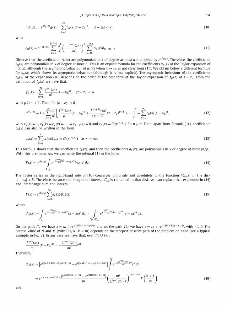
Observe that the coefficients An(x) are polynomials in x of degree at most n multiplied by exf (z0) . Therefore, the coefficientsan(x) are polynomials in x of degree at most n. This is an explicit formula for the coefficients an(x) of the Taylor expansion ofh(z, x), although the asymptotic behaviour of an(x) when x → ∞ is not clear from (11). We obtain below a different formulafor an(x) which shows its asymptotic behaviour (although it is less explicit). The asymptotic behaviour of the coefficientsan(x) of the expansion (10) depends on the order of the first term of the Taylor expansion of f p(z) at z = z0. From thedefinition of f p(z) we have that:

f p(z) =∞∑

n=p

f (n)(z0)

n! (z − z0)n, |z − z0| < R,

with p � m + 1. Then, for |z − z0| < R ,

exfm(z) = 1 +∞∑

n=1

xn

n![

f (p)(z0)

p! (z − z0)p + f (p+1)(z0)

(p + 1)! (z − z0)p+1 + · · ·

]n

=∞∑

n=0

cn(x)(z − z0)n, (12)

with c0(x) = 1, c1(x) = c2(x) = · · · = cp−1(x) = 0 and cn(x) = O(x n/p�) for n � p. Then, apart from formula (11), coefficientsan(x) can also be written in the form

an(x) =n∑

k=0

ck(x)Bn−k = O(x n/p�) as x → ∞. (13)

This formula shows that the coefficients cn(x), and then the coefficients an(x), are polynomials in x of degree at most [n/p].With this preliminaries, we can write the integral (1) in the form

F (x) ∼ exf (z0)

∫Γz0

exf (m)(z0)

m! (z−z0)mh(z, x)dz. (14)

The Taylor series in the right-hand side of (10) converges uniformly and absolutely to the function h(z, x) in the disk|z − z0| < R . Therefore, because the integration interval Γz0 is contained in that disk, we can replace that expansion in (14)and interchange sum and integral:

F (x) ∼ exf (z0)

∞∑n=0

an(x)Φn(x), (15)

where

Φn(x) :=∫

Γz0

exf (m)(z0)

m! (z−z0)m(z − z0)

n dz ∼∫

ΓN ∪ΓM

exf (m)(z0)

m! (z−z0)m(z − z0)

n dz.

On the path ΓN we have z = z0 + rei[(2N+1)π−φ]/m and on the path ΓM we have z = z0 + rei[(2M+1)π−φ]/m , with r � 0. Theprecise value of N and M (with 0 � N, M < m) depends on the steepest descent path of the problem on hand (see a typicalexample in Fig. 2). In any case we have that, over ΓN ∪ ΓM :

f (m)(z0)

m! (z − z0)m = −| f (m)(z0)|

m! rm.

Therefore,

Φn(x) ∼ [ei[(2N+1)π−φ](n+1)/m − ei[(2M+1)π−φ](n+1)/m] ∞∫

0

e−x| f (m)(z0)|

m! rmrn dr

= ei[π−φ](n+1)/m [e2Niπ(n+1)/m − e2Miπ(n+1)/m]m

(m!

| f (m)(z0)|x)(n+1)/m

Γ

(n + 1

m

)(16)

and

352 J.L. López et al. / J. Math. Anal. Appl. 354 (2009) 347–359

Table 1Every entrance of this table represents (k, O(akΦk)) for the particular example m = 3 and p = 5. We group the terms akΦk of the expansion (15) inblocks of p = 5 terms. Every row of the table contains one of those blocks. In every column, the terms akΦk are of the same order, and sum up thecorresponding Ψn . From the third column to the right, odd columns contain n/2� − (n − 3)/2� + 1 = 2 terms (Ψn is the sum of two terms akΦk for oddn) and even columns contain n/2� − (n − 3)/2� + 1 = 3 terms (Ψn is the sum of three terms akΦk for even n).

Ψ0 Ψ1 Ψ2 Ψ3 Ψ4 Ψ5 Ψ6 Ψ7 Ψ8 Ψ9

0, x0 1, x−1/3 2, x−2/3 3, x−1 4, x−4/3

5, x−2/3 6, x−1 7, x−4/3 8, x−5/3 9, x−2

10, x−4/3 11, x−5/3 12, x−2 13, x−7/3 14, x−8/3

15, x−2 16, x−7/3 17, x−8/3 18, x−3

19, x−8/3 20, x−3

F (x) ∼ exf (z0)

∞∑n=0

an(x)ei[π−φ] n+1m

[e2Niπ n+1m − e2Miπ n+1

m ]m

Γ

(n + 1

m

)∣∣∣∣ m!f (m)(z0)x

∣∣∣∣n+1

m

. (17)

We can see that Φn(x) is of the order O(x−(n+1)/m) as x → ∞. Therefore, the terms of the expansion (15) satisfyan(x)Φn(x) = O(x n/p�−(n+1)/m). Then, the expansion (15) (and the expansion (17)) is not a genuine asymptotic expansion.But we can group the terms of (15) in such a way that we get a generalized asymptotic expansion:

F (x) = exf (z0)

∞∑n=0

Ψn(x), (18)

with

Ψn(x) := n/(p−m)�∑

k= (n−m)/(p−m)�an+mk(x)Φn+mk(x) = O

(x−(n+1)/m)

, x → ∞. (19)

In this sum, −n� with n natural must be understood as zero. Observe that we have grouped the terms ak(x)Φk(x) of (15)in blocks Ψn(x) of n/(p − m)� − (n − m)/(p − m)� + 1 terms ak(x)Φk(x). Table 1 represents the orders of the first fewterms ak(x)Φk(x) of the expansion (15) (multiplied by x1/m) for the particular case m = 3 and p = 5.

Observation 1. The terms an(x) are polynomials of degree at most n/p�. Then, from (19) we see that the asymptoticsequence Ψn(x) is simply a sum of n/(p − m)� − (n − m)/(p − m)� + 1 negative powers of x.

We can resume the above discussion in the following theorem.

Theorem 1. Consider the paths C , Γ = Γz0 ∪ Γε and Γz0 ⊂ ΓN ∪ ΓM explained above. Let the functions f (z) and g(z) in (1) beanalytic in a connected open domain containing the paths C and Γ and suppose that the integral (1) exists for x � x0 . Let z0 be theunique saddle point of f (z) on Γ . Then, as x → ∞,

F (x) ∼ exf (z0)

∞∑n=0

ei(π−φ)(n+1)/m e2iπ N(n+1)/m − e2iπ M(n+1)/m

mΨn(x), (20)

Ψn(x) := n

p−m �∑k= n−m

p−m �ei(π−φ)kan+mk(x)Γ

(k + n + 1

m

)∣∣∣∣ m!f (m)(z0)x

∣∣∣∣k+(n+1)/m

. (21)

In this sum, −n� with n natural must be understood as zero and φ = arg( f (m)(z0)). The integer m is the degree of the first non-vanishing derivative of f (z) at z = z0 and p is the degree of the next non-vanishing derivative. The integers N and M depend on the

steepest descent path ΓN ∪ ΓM chosen for fm(z) = f (z) − f (m)(z0)m! (z − z0)

m and 0 � N, M � m − 1 (see Fig. 1). For n = 0,1,2, . . . ,

an(x) := e−xf (z0)

n/m�∑k=0

xk

k!(

− f (m)(z0)

m!)k

×n−mk∑

j=0

A j(x)Bn−mk− j, (22)

where A j(x) and B j are the Taylor coefficients at z = z0 of exf (z) and g(z) respectively:

exf (z) =∞∑

n=0

An(x)(z − z0)n, g(z) =

∞∑n=0

Bn(z − z0)n, |z − z0| < R,

with Γz0 ⊂ D R(z0). The terms of the expansion are of the order Ψn(x) = O(x−(n+1)/m) as x → ∞.

J.L. López et al. / J. Math. Anal. Appl. 354 (2009) 347–359 353

Fig. 3. The paths C , Γ = Γz0 ∪ Γε , Γ̃ and Γz0 ⊂ Γ0 ∪ Γ1 involved in the saddle point approximation of the Airy function. The paths Γz0 and Γε join at thepoints z = 1 ± i

√3.

3. Examples

3.1. The Airy function Ai(x) for large x

From [8, p. 90, Eq. (4.22)] we have

Ai(x) =√

x

2π i

∫C

ex3/2[ 13 z3−z] dz,

where C is any contour which begins at infinity in the sector −π/2 < arg(z) < −π/6 and ends at infinity in the sectorπ/6 < arg(z) < π/2 (see Fig. 3). This integral has the form (1) with f (z) = 1

3 z3 − z and g(z) = 1. We consider x > 0 large.The functions f (z) and g(z) are analytic in the whole complex plane. The two critical points of f (z) are ±1 and theasymptotically relevant one is z0 = 1. We have f (1) = −2/3, f ′′(1) = 2 and f ′′′(1) �= 0. With the notation of the precedingsection we have m = 2, p = 3 and φ = 0. In particular, f3(z) = 1

3 (z − 1)3.

The function h(z, x) = ex3/2 f3(z) g(z) has the following Taylor expansion at z = 1:

h(z, x) = ex3/2

3 (z−1)3 =∞∑

n=0

x3n/2

3nn! (z − 1)3n,

with radius of convergence R = ∞. Therefore, with the notation of the preceding section we have

a3n+1(x) = a3n+2(x) = 0 and a3n(x) = x3n/2

3nn! for n = 0,1,2, . . . . (23)

It is evident that an(x) is a polynomial of degree not greater than n/3� in the variable x3/2.The steepest descent path of the function f2(z) = −2/3+ (z −1)2 through z0 = 1 is a vertical straight line through z0 = 1

(N = 0, M = 1):

Γ0 ∪ Γ1 = {z ∈ C, z = 1 ± ir, r � 0}.We chose Γz0 to be a subinterval of Γ0 ∪ Γ1 containing z0: Γz0 = {1 + iy, y ∈ [−√

3,√

3 ]}. We choose Γε to be the twostraight lines joining the ends of Γz0 with the infinity with at angle of π/3 and −π/3 respectively: Γε = {(1 ± i

√3)t ,

1 � t < ∞} (see Fig. 3). Then, the path Γ considered in the previous section is the union of these two paths: Γ = Γz0 ∪ Γε .It is evident that the path C can be deformed to the path Γ :

Ai(x) =√

x

2π i

∫Γ

ex3/2[ 13 z3−z] dz.

Moreover, over Γε we have that

∫Γε

ex3/2[ 13 z3−z] dz = 2

{e−11x3/2/3

∞∫1

e[11/3−8t3/3−t−i√

3t]x3/2dt

}= O

(e−11x3/2/3).

On the other hand, it is clear that

354 J.L. López et al. / J. Math. Anal. Appl. 354 (2009) 347–359

∫Γz0

ex3/2[ 13 z3−z] dz = O

(e−2x3/2/3)

and then

Ai(x) ∼√

x

2π i

∫Γz0

ex3/2[ 13 z3−z] dz. (24)

From (20)–(23) we have that an asymptotic expansion of Ai(x) for large x is

Ai(x) ∼ e−2x3/2/3

2π

∞∑n=0

(−1)nΓ (3n + 1/2)

9n(2n)!x3n/2+1/4. (25)

This is just the asymptotic expansion obtained by using the standard saddle point method [8, Chapter 2, Example 7],although this derivation is simpler. This is a very easy example and both methods give the same expansion; the followingexamples are not so trivial and the expansions differ from the ones obtained using the standard saddle point method.

3.2. The Hankel function H(1)n (x) for large n and x. The case 0 < α < 1

From [8, p. 94, Example 8] we have:

H(1)x (αx) = 1

π i

∞+π i∫−∞

exf (z) g(z)dz,

with f (z) = α sinh z − z and g(z) = 1. We consider x and α positive with α fixed and x large. The function f (z) is analyticon the whole complex plane. The saddle points z0 of f (z) are points z0 satisfying α cosh z0 = 1. In the region −π < z < π ,there are two real saddle points if 0 < α < 1, two purely imaginary saddle points if α > 1 and only one saddle point atz0 = 0 if α = 1.

When 0 < α < 1, the saddle points z0 are the two real solutions (one positive and the other one negative) ofα cosh z0 = 1. The relevant one is the negative solution: z0 = −| cosh−1(1/α)|. We have f (z0) = | cosh−1(1/α)| − √

1 − α2,f ′′(z0) = −√

1 − α2 and f ′′′(z0) �= 0. With the notation of the preceding section we have m = 2, p = 3 and φ = π . In par-ticular, f2(z) = | cosh−1(1/α)| − √

1 − α2 − 12

√1 − α2(z − z0)

2 and f3(z) = f (z) − f2(z). The function h(z, x) = exf3(z) has aTaylor expansion at z = z0:

exf (z) = e−xzeαx sinh z =∞∑

n=0

An(x)(z − z0)n, (26)

with A0(x) = ex(α sinh z0−z0) and, for n = 0,1,2, . . . ,

An+1(x) = −xAn(x) + αx cosh z0

n/2�∑k=0

An−2k(x)

(2k)! + αx sinh z0

(n−1)/2�∑k=0

An−2k−1(x)

(2k + 1)! . (27)

The coefficients An follow after substitution of the expansion (26) into the differential equation y′ − x(α cosh z − 1)y = 0satisfied by the function y(z) = exf (z) . On the other hand,

ex2

√1−α2(z−z0)2 =

∞∑k=0

1

k!(

x√

1 − α2

2

)k

(z − z0)2k.

The common radius of convergence of these expansions is R = ∞. Eq. (22) reads

an(x) = e−xf (z0)

n/2�∑k=0

xk

k!(√

1 − α2

2

)k

An−2k(x), (28)

with An(x) given by the recursion (27).The steepest descent path of the function f2(z) through z0 is the real axis, Γ0 ∪ Γ1 = R (N = 0 and M = 1). We take as

Γz0 the negative real axis Γz0 = R− and as Γε the interval of the imaginary axis joining the origin and the point iπ and the

horizontal straight line joining the point iπ with the infinity: Γε = {iy, 0 � y � π} ∪ {iπ + t , 0 � t < ∞} (see Fig. 4). Then,the path Γ considered in the previous section is the union of these two paths: Γ = Γz0 ∪ Γε . It is clear that the path C canbe deformed to the path Γ :

J.L. López et al. / J. Math. Anal. Appl. 354 (2009) 347–359 355

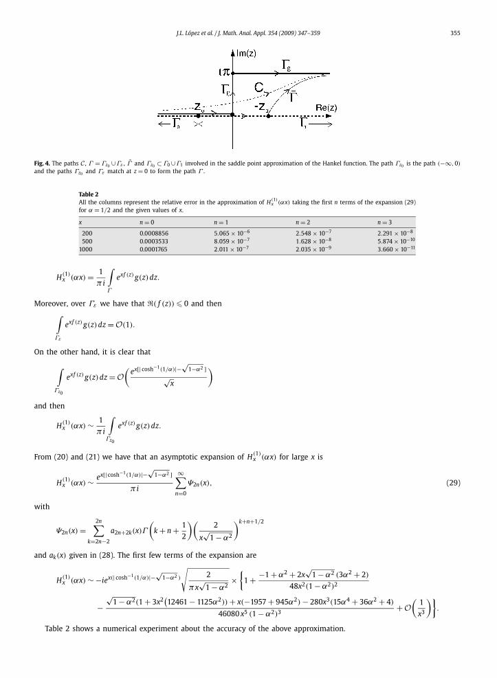
Fig. 4. The paths C , Γ = Γz0 ∪Γε , Γ̃ and Γz0 ⊂ Γ0 ∪Γ1 involved in the saddle point approximation of the Hankel function. The path Γz0 is the path (−∞,0)

and the paths Γz0 and Γε match at z = 0 to form the path Γ .

Table 2All the columns represent the relative error in the approximation of H(1)

x (αx) taking the first n terms of the expansion (29)for α = 1/2 and the given values of x.

x n = 0 n = 1 n = 2 n = 3

200 0.0008856 5.065 × 10−6 2.548 × 10−7 2.291 × 10−8

500 0.0003533 8.059 × 10−7 1.628 × 10−8 5.874 × 10−10

1000 0.0001765 2.011 × 10−7 2.035 × 10−9 3.660 × 10−11

H(1)x (αx) = 1

π i

∫Γ

exf (z) g(z)dz.

Moreover, over Γε we have that ( f (z)) � 0 and then∫Γε

exf (z) g(z)dz = O(1).

On the other hand, it is clear that

∫Γz0

exf (z) g(z)dz = O(

ex[| cosh−1(1/α)|−√

1−α2 ]√

x

)

and then

H(1)x (αx) ∼ 1

π i

∫Γz0

exf (z) g(z)dz.

From (20) and (21) we have that an asymptotic expansion of H (1)x (αx) for large x is

H(1)x (αx) ∼ ex[| cosh−1(1/α)|−

√1−α2 ]

π i

∞∑n=0

Ψ2n(x), (29)

with

Ψ2n(x) =2n∑

k=2n−2

a2n+2k(x)Γ

(k + n + 1

2

)(2

x√

1 − α2

)k+n+1/2

and ak(x) given in (28). The first few terms of the expansion are

H(1)x (αx) ∼ −iex(| cosh−1(1/α)|−

√1−α2 )

√2

πx√

1 − α2×

{1 + −1 + α2 + 2x

√1 − α2 (3α2 + 2)

48x2(1 − α2)2

−√

1 − α2(1 + 3x2(12461 − 1125α2)) + x(−1957 + 945α2) − 280x3(15α4 + 36α2 + 4)

46080 x5 (1 − α2)3+ O

(1

x3

)}.

Table 2 shows a numerical experiment about the accuracy of the above approximation.

356 J.L. López et al. / J. Math. Anal. Appl. 354 (2009) 347–359

Fig. 5. The paths C , Γ = Γz0 ∪ Γε , Γ̃ and Γz0 ⊂ Γ0 ∪ Γ1 involved in the saddle point approximation of the Hankel function for α > 1. The path Γz0 is thepath [z1, z2] and the paths Γz0 and Γε join at z1 = −|z0| and z2 = π − |z0| + iπ to form the path Γ .

3.3. The Hankel function H(1)n (x) for large n and x. The case α > 1

The saddle points z0 are the two purely imaginary solutions of the equation α cosh z0 = 1: ±i| cosh−1(1/α)|. The relevantsaddle point is: z0 = i| cosh−1(1/α)|. We have f (z0) = i

√α2 − 1 − i| cosh−1(1/α)|, f ′′(z0) = i

√α2 − 1 and f ′′′(z0) �= 0. With

the notation of the preceding section we have m = 2, p = 3 and φ = π/2. In particular, f2(z) = i√

α2 − 1− i| cosh−1(1/α)|+i√

α2−12 (z − z0)

2 and f3(z) = f (z) − f2(z). The function h(z, x) = exf3(z) has the Taylor expansion at z = z0 given in (27) and

e−xf2(z) = e−xf (z0)

∞∑k=0

1

k!(−ix

√α2 − 1

2

)k

(z − z0)2k.

The common radius of convergence of these expansions is R = ∞. Eq. (22) reads

an(x) = e−xf (z0)

n/2�∑k=0

xk

k!(

− i√

α2 − 1

2

)k

An−2k(x), (30)

with An(x) defined in (27).The steepest descent path of the function f2(z) is a straight line through z0 forming an angle of π/4 with the imaginary

axis (N = 0 and M = 1, see Fig. 5):

Γ0 ∪ Γ1 = {z ∈ C, z = z0 + (1 + i)t, t ∈ R

}.

We choose Γz0 to be the interval of Γ0 ∪ Γ1 located between the X axis and the horizontal straight line z = iπ (thatobviously contains the point z0); that is, Γz0 = {z ∈ C, z = z0 + (1 + i)t, −|z0| � t � π − |z0|}. We choose Γε to be the twohorizontal straight lines joining the ends of Γz0 with the infinity (see Fig. 5), that is, Γε = {t ∈ R,−∞ < t < −|z0|} ∪ {z ∈C, z = t + iπ,π − |z0| < t < ∞}. Then, the path Γ considered in the previous section is the union of these two paths:Γ = Γz0 ∪ Γε . It is clear that the path C can be deformed to the path Γ :

H(1)x (αx) = 1

π i

∫Γ

exf (z) g(z)dz.

Moreover, over Γε we have that ( f (z)) � M0 := Max{α sinh(|z0| − π) + |z0| − π, |z0| − α sinh |z0|} < 0 and then∫Γε

exf (z) g(z)dz = O(e−xM0

).

On the other hand, it is clear that

∫Γz0

exf (z) g(z)dz = O(

eix[√

α2−1−| cosh−1(1/α)|]√

x

)= O

(1√

x

)

and then

H(1)x (αx) ∼ 1

π i

∫Γz0

exf (z) g(z)dz.

From (20) and (21) we have that an asymptotic expansion of H (1)x (αx) for large x is

J.L. López et al. / J. Math. Anal. Appl. 354 (2009) 347–359 357

Table 3All the columns represent the relative error in the approximation of H(1)

x (αx) taking the first n terms of the expansion (31)for α = 2 and the given values of x.

x n = 0 n = 1 n = 2 n = 3

200 0.00056130 2.182 × 10−6 1.891 × 10−8 1.737 × 10−10

500 0.00022452 3.492 × 10−7 1.210 × 10−9 4.449 × 10−12

1000 0.00011226 8.731 × 10−8 1.512 × 10−10 2.868 × 10−13

H(1)x (αx) ∼ eix[

√α2−1−| cosh−1(1/α)|]

π i

∞∑n=0

eiπ(2n+1)/4Ψ2n(x) (31)

with

Ψ2n(x) =2n∑

k=2n−2

ika2n+2k(x)Γ

(k + n + 1

2

)(2

x√

α2 − 1

)k+n+1/2

and an(x) given in (30). The first few terms of the expansion are

H(1)x (αx) ∼ e−iπ/4eix(

√α2−1−| cosh−1(1/α)|)

√2

πx√

α2 − 1×

{1 − 1 − α2 + 2xi

√α2 − 1 (3α2 + 2)

48x2(α2 − 1)2

+ i√

α2 − 1(1 − 3x2(12461 − 1125α2)) + x(−1957 + 945α2) − 280x3(15α4 + 36α2 + 4)

46080x5(α2 − 1)3+ O

(1

x3

)}.

Table 3 shows a numerical experiment about the accuracy of the above approximation.

3.4. The Hankel function H(1)n (x) for large n and x. The case α = 1

When α = 1 there is only one saddle point z0 = 0. We have f (0) = 0, f ′′(0) = 0, f ′′′(z0) = 1, f (iv)(0) = 0 and f (v)(0) �= 0.With the notation of the preceding section we have m = 3, p = 5 and φ = 0. In particular, f3(z) = z3/6 and f5(z) =f (z) − f3(z). The function h(z, x) = exf5(z) has a Taylor expansion at z = 0:

exf (z) =∞∑

n=0

An(x)zn, (32)

with A0(x) = 1 and

An+1(x) = x n/2�∑k=0

An−2k(x)

(2k)! − xAn(x), n = 0,1,2, . . . . (33)

On the other hand,

e−xf3(z) = e−xz3/6 =∞∑

k=0

1

k!(

− x

6

)k

z3k.

The coefficients An follow after substitution of the expansion (32) into the differential equation y′ − x(cosh z − 1)y = 0satisfied by the function y(z) = exf (z) . The common radius of convergence of these expansions is R = ∞. Eq. (22) reads

an(x) = n/3�∑k=0

xk

k!(

−1

6

)k

An−3k(x), (34)

with An(x) defined in (33).The steepest descent paths of the function f3(z) through z0 = 0 are the three semi-straight lines

Γ0 = {t + it, t > 0}, Γ1 = {t, t < 0}, Γ2 = {t − it, t > 0}.We take Γ0 and Γ1 (N = 0, M = 1) and discard Γ2. The path Γz0 consists of the whole Γ1 plus that piece of Γ0 located

between the X axis ant the horizontal straight line z = iπ : Γz0 = R− ∪ {z ∈ C, z = t(1 + i), 0 � t � π}. The path Γε is the

horizontal straight line joining the point π + iπ with the infinity: Γε = {t + iπ , π < t < ∞} (see Fig. 6). Then, the path Γ

considered in the previous section is the union of these two paths: Γ = Γz0 ∪Γε . It is clear that the path C can be deformedto the path Γ :

358 J.L. López et al. / J. Math. Anal. Appl. 354 (2009) 347–359

Fig. 6. The paths C , Γ = Γz0 ∪ Γε , Γ̃ and Γz0 ⊂ Γ0 ∪ Γ1 involved in the saddle point approximation of the Hankel function for α = 1. The path Γz0 is thepath (−∞,0] ∪ [0, z∗] and the paths Γz0 and Γε join at z∗ = π + iπ to form the path Γ .

Table 4All the columns represent the relative error in the approximation of H(1)

x (αx) taking the first n terms of the expansion (35)for α = 1 and the given values of x.

x n = 0 n = 4 n = 6 n = 10

200 0.0000111 1.111 × 10−7 2.304 × 10−11 1.005 × 10−12

500 3.297 × 10−6 1.777 × 10−8 1.091 × 10−12 2.545 × 10−14

1000 1.309 × 10−6 4.444 × 10−9 1.085 × 10−13 1.250 × 10−15

H(1)x (x) = 1

π i

∫Γ

exf (z) g(z)dz.

Moreover, over Γε we have that ( f (z)) � − sinhπ − π and then∫Γε

exf (z) g(z)dz = O(e−x(sinhπ+π)

).

On the other hand, it is clear that∫Γz0

exf (z) g(z)dz = O(

1

x1/3

)

and then

H(1)x (x) ∼ 1

π i

∫Γz0

exf (z) g(z)dz.

From (20) and (21) we have that an asymptotic expansion of H (1)x (x) for large x is

H(1)x (x) ∼ 1

π i

∞∑n=0

(−1)n + eiπ(n+1)/3

3Ψn(x), (35)

with

Ψn(x) = n/2�∑

k= (n−3)/2�(−1)kan+3k(x)Γ

(k + n + 1

3

)(6

x

)k+(n+1)/3

and an(x) given in (34). The first few terms of the expansion are

H(1)x (x) = 1

3π i

(6

x

)1/3

×{(

1 + eiπ/3)Γ (1

3

)+ 3

1 + ei5π/3

1400Γ

(8

3

)(6

x

)4/3

− (1 + eiπ/3)Γ ( 103 )(1 + 49896z2)

11642400z4+ O

(1

x7/3

)}.

Table 4 shows a numerical experiment about the accuracy of the above approximation.

J.L. López et al. / J. Math. Anal. Appl. 354 (2009) 347–359 359

4. Concluding remarks

The standard saddle point method of asymptotic expansions of integrals requires the proof of the existence of the (usuallycomplicated) steepest descent paths and an inversion problem associated to a change of variables. These two technical pointsmake difficult the construction of an explicit and systematic (universal) formula for the expansion (although we can findsome more or less explicit formulas in the literature that simplify the computation of the coefficients of the expansion).

We have proposed a variant of the saddle point method which makes the computation of the complete expansionstraightforward and systematic: an asymptotic expansion of F (x) for large x is given in Theorem 1, formula (20), with Ψn(x)given in (21). In these formulas, the integers m, p, M and N are related to the order of the saddle point z0 and the steepestdescent straights chosen. The polynomials an(x) are given explicitly in (22) in terms of the Taylor coefficients of g(z) andexp[xf (z)] at z = z0. Once the saddle point z0 is found and the integers m, p, M and N are computed, these formulas areeasily implementable on a symbolic manipulation program like Mathematica or Maple for example to compute the wholeasymptotic expansion.

With this new procedure, the steepest descent contour is universal: the union of two straight lines and the phase func-tion is always a polynomial: f (z0) plus a power of z − z0, where z0 is the saddle point of the phase function. On the otherhand, the remaining integrand h(z, x) is a function not only of the integration variable z, but also of the asymptotic variablex. As a consequence, and as difference with respect to the standard saddle point method, the asymptotic expansion (20) isa generalized asymptotic expansion, not a Poincaré expansion. Although it is very simple: the asymptotic sequence Ψn(x)consists of the sum of a few negative powers of x (it is almost Poincaré).

We have applied the method to the important example of the Hankel function, obtaining new and simple asymptoticexpansions of this function when both, its variable and degree are large. The method can be applied to many other specialfunctions, including orthogonal polynomials, and we believe that new and simple asymptotic expansions can be obtained.

Acknowledgments

We thank Professor Nico Temme for his helpful comments and suggestions. The Dirección General de Ciencia y Tecnología (REF. MTM2007-63772) and theGobierno of Navarra (REF. 2008/2301) are acknowledged by their financial support.

References

[1] Berry, Howls, Hyperasymptotics for integrals with saddles, Proc. R. Soc. Lond. Ser. A 443 (1991) 657–675.[2] J.A. Campbell, P.O. Fröman, E. Walles, Explicit series formulae for the evaluation of integrals by the method of steepest descent, Stud. Appl. Math. 77

(1987) 151–172.[3] A. Erdélyi, Asymptotic Expansions, Dover Publications, Inc., New York, 1956.[4] C. Ferreira, J.L. López, P. Pagola, Ester Pérez Sinusía, The Laplace’s and steepest descents methods revisited, Int. Math. Forum 2 (7) (2007) 297–314.[5] F.W.J. Olver, Why steepest descents, SIAM Rev. 12 (1970) 228–247.[6] F.W.J. Olver, Asymptotic and Special Functions, AKP Classics, 1997.[7] O. Perron, Über die näherungsweise Berechnung von Funktionen großber Zahlen, Sitzungsber. Bayr. Akad. Wiss. Münch. Ber. (1917) 191–219.[8] R. Wong, Asymptotic Approximations of Integrals, Academic Press, New York, 1989.