A Study of Trends in India’s Economic Growth since 1951: The

Inclusive Growth Approach

Arjun. Y. Pangannavar *

ABSTRACT

This paper focuses on the saga of India’s economic growth under the ‘Nehru-

Mahalanobis Economic Growth Model’ (NMEGM) and ‘Narsimhrao-Manmohan Singh

Economic Growth Model’ (NMSEGM). The NMEGM continued till 1990 unceasingly;

Indira Gandhi’s social control had supported the model to place India’s economic

growth at a high level. After becoming a member of World trade Organization (WTO),

India entered the epoch of world new economic order and initiated new economic

reforms. It followed globalisation, liberalisation and privatisation policies to achieve

double digit economic growth rate. This model is popularly known as ‘Narsimhrao-

Manmohan Singh Economic Growth Model’. Based on past trends and new changes, this

paper attempts to assess the impact of NMSEGM on future economic growth. India has

practiced both endogenous and exogenous models of economic growth. The endogenous

model was in operation from 1956-57 till 1990-91 that placed economic growth rate at

more than 5%. However, from 1990-91, the new economic reforms have followed the

exogenous model that has raised economic growth rate to nearing double-digit; but, the

decadal economic growth rate has shown a declining trend. This paper attempts to

assess the growth rate trends of Indian economy by using the measuring tool called

‘Inclusive Growth’ to get a fair and true picture.

Keywords: Economic Growth Models, Indian GNP, Inclusive Growth, NMSEGM,

NMEGM, Human Capital Investment, Natural Capital Investment.

1.0. Introduction

A number of research studies have been conducted by economists on economic

growth in general and country-wise economic growth in particular. They have

generated knowledge about the economic-growth-concept, its determinants,

measurement, policy and effects.

_________________

*Associate Professor of Economics, JSS Arts, Science & Commerce College, Gokak, Karnataka.

Trends in India’s Economic Growth since 1951: The Inclusive Growth Approach 21

The main determinants of economic growth have undergone changes as per the

requirement of the changing context and thinking; the environment has to be assigned

paramount position in defining ‗economic growth‘ in the present-day context.

1.1 Statement of problem

The economic growth concept has undergone change to suit the present day

changes and requirements. Gross Domestic Product (GDP) or Gross National Product

(GNP) is not the sufficient indicator to define or measure the economic growth of a

country, poor and rich. The economic growth has to be included with the growth of

resources including environment factor. The economic growth should take place not at

the cost of or by depleting the natural resources but it should be accompanied with the

growth of natural resources as well as maintaining ecological balance in the economy.

GNP growth inclusive of natural resources growth along with ecological balance must

be the measure of economic growth rate. The empirical research approach is used to

study the trends, the causes and impact of economic growth of India since 1951.

1.2 Importance and objectives of the study

The traditional measurement of economic growth rate is no longer enough as

it does not take into account the importance of environmental protection, human

capitalisation and population growth aspects while computing growth trends. In the

present day context, these aspects have become relevant because in many cases,

higher economic growth is being achieved at the cost of environmental degradation

and human rights violation. Thus, there is need for redefining the term ‗economic

growth‘ by giving importance to environment-protection and thereby natural capital

growth. This study attempts to fill this measurement gap. The main objective of this

paper is to assess India‘s economic growth during 1951-52 to 2010-2011 and find out

if it is broad-based and inclusive.

2.0 Review of Literature

There are different views on the meaning of ‗economic growth‘ but it is mainly

concerned with the changes in a nation‘s GNP over the specific period of time,

generally a year. The GNP comprises the total value of total production of goods and

services produced from different sectors of economy by using resources and

technology (IMF, 2012). It can be estimated or calculated either in terms of constant

price or market/current price. If it is calculated in terms of constant/base year price, it

is known as ‗Real Economic Growth (REG)‘. If it is calculated in terms of

22 PRAGATI: Journal of Indian Economy, Vol. 2, Issue 1

current/market price, it is known as ‗Nominal Economic Growth (NEG)‘. The real

economic growth gives real picture of the achievement of the economy with success

or failure of either governance or policies or both. The difference between REG and

NEG gives the extent of inflationary situation in the economy.

The economic concept of growth is as old as human civilization. In Indian Vedic

period, we find a mention of this concept in Valmiki‘s Ramayana, a great epic of the

world, as Vedic values of want/desire(kaam), wealth (arth), policy (dharm/ Religion)

and salvation/satisfaction (moksha). The emperors and kings used to worship the

‗Goddess of Wealth‘ (Lakshmi) to improve nation‘s wealth in terms of production, assets

and resources. These things also find a mention in Kautilya‘s ‗Principles of Political

Economy‘ (Arth Shastra). In 1377, Ibn Khaldun, the Arabian economic thinker,

had provided one of the earliest descriptions of economic growth in his famous

Muqaddimah, which is known as ‗Prolegomena‘ in the Western world.

In the early modern period, some people in Western European nations had developed

the idea of ‗economic growth‘; that is, to produce a greater economic surplus which

could be expended on something other than mere subsistence. This surplus could then be

used for consumption, warfare, or civic and religious projects. The previous view was

that only increasing either population or tax rates could generate more surplus money for

the Crown or country to achieve economic growth (Erber & Hagemann, 2002).

The concept of ‗economic growth‘ is a long-run process which indicates increase in

total national output/income in long-run. The short-run fluctuations in national-output

are considered as ‗business cycles‘; so economists draw a distinction between short-term

economic stabilization and long-term economic growth (Barro, 1997). The concept

‗economic growth‘ is different from the concept ‗economic development‘: economic

growth is a narrow concept because it focuses on only national output but economic

development is broad concept because it focuses on national output as well as quality of

life. An increase in growth caused by more efficient use of inputs is referred to as

intensive growth. GDP growth caused only by increases in inputs such as capital,

population or territory is called extensive growth (Bjork, 1999). However, now it is

generally recognised that economic growth also corresponds to a process of continual

rapid replacement and reorganisation of human activities facilitated by investment and

motivated to maximise returns.

In the course of time a good number of theories have developed to explain the causes

and effects of economic growth and measurement of economic growth rate. The

mercantilists‘ ‗Bullionist Theory of Economic growth‘, during the early modern times,

had considered economic growth as increase in total amount of gold and silver under

state-control through expansion of trade and creation of colonies abroad. Later, the

Trends in India’s Economic Growth since 1951: The Inclusive Growth Approach 23

‗Bullionist Theory‘ supported increase the producing capacity of manufacturing

industries, so as to boost their exports abroad at low-price and avoid foreign competition

with a view to establish their trade supremacy abroad. Under this theory of growth, the

road to increased national wealth was to grant monopolies, for instance Dutch East India

company, and British East India company. This would give an incentive for an

individual to exploit a market or resource, confident that he would make all of the profits

when all other extra-national competitors were driven out of business. This theory was

unacceptable because of its ‗tit for tat policy‘ that begets wars among the nations. The

Physiocrats, Scottish Enlightenment Thinkers such as David Hume and Adam Smith

criticised the mercantilists‘ theory of growth and begot the modern concept of economic

growth; the rise of ‗Classical Economic Growth Theory‘ and foundation of Modern

Political Economics‘. The theory of the Physiocrats was that productive capacity, itself,

allowed for growth, and thus there should be increasing capital to allow that capacity i.e.

‗the wealth of nations‘. These classical economists stressed the importance of agriculture

and saw urban industry as ‗sterile‘. Smith extended the notion that manufacturing was

central to the entire economy and capital formation and division of labour as causal

factors of economic growth. David Ricardo would then argue that trade was a benefit to

a country, because if one could buy a good more cheaply from abroad, it meant that there

was more profitable work to be done here. This theory of ‗comparative advantage‘

would be the central basis for arguments in favour of free trade as an essential

component of growth. However, the growth in income per capita was essentially flat

until the Inudustrial Revolution. Thomas Malthus in his ‗Essay on the Principle of

Population‘ said that ―any growth in the economy would translate into a growth in

population.‖ The mainstream theory of economic growth states that with the industrial

revolution and advancements in medicine, life expectation increased, infant mortality

decreased, and the payoff to receiving an education was higher. Thus, parents began to

place more value on the quality of their children and not on the quantity. This led to a

drop in the fertility rates of most industrialised nations. This is known as the breakdown

of the Malthusian regime. With income increasing faster than population growth,

industrialised economies substantially increased their incomes per capita in the next

centuries. Thus, although aggregate income could increase, income per capita was bound

to stay roughly constant. In brief, the classical theory of production and the theory of

growth are based on the theory or law of variable proportions, whereby increasing either

of the factors of production viz. labor and capital, while holding the other constant and

assuming no technological change, will increase output, but at a diminishing rate that

eventually will approach zero. These concepts have their origins in Thomas Malthus‘s

theorising about agriculture. Malthus‘s examples included the number of seeds harvested

24 PRAGATI: Journal of Indian Economy, Vol. 2, Issue 1

relative to the number of seeds planted (capital) on a plot of land and the size of the

harvest from a plot of land versus the number of workers employed. Criticisms of

classical growth theory are that technology, the most important factor in economic

growth, is held constant and the economies of scale are ignored (Foley, 1999).

The Harrod–Domar Model was an early post- Keynesian model of economic

growth. The model was developed independently by Roy F. Harrod (1939) and Evsey

Domar (1946). The Harrod–Domar model was initially created to analyse the business

cycles, it was later adapted to explain economic growth. Its implications were that

growth depends on the quantity of labour and capital; more investment leads to capital

accumulation, which generates economic growth. The model carries implications for less

economically developed countries, where labour is in plentiful supply in these countries

but physical capital is not, slowing down economic progress (Jones, 2002). It is used in

developing countries to explain an economy's growth rate in terms of the level of saving

and productivity of capital. It suggests that there is no natural reason for an economy to

have balanced growth. In brief, the model implies that economic growth depends on

policies to increase investment, by increasing saving, and using that investment more

efficiently through technological advances. The Harrod–Domar model mentioned three

kinds of growth viz. warranted growth, actual growth and natural rate of growth. The

model concludes that an economy does not ‗naturally‘ find full employment and stable

growth rates. The main criticism of the model is the level of assumption, one being that

there is no reason for growth to be sufficient to maintain full employment; this is based

on the belief that the relative price of labour and capital is fixed, and that they are used in

equal proportions. Perhaps the most important parameter in the Harrod–Domar model is

the rate of savings but the model fails to explain the distribution of income which

determines the per capita income that influences on rate of savings. The neoclassical

economists claimed shortcomings in the Harrod–Domar model, and, by the late 1950s,

started an academic dialogue that led to the development of the Solow–Swan model.

According to ‗Neo-Classical Economic Growth Theory‘ the notion of growth is

increased stocks of capital goods, which is popularly known as the ‗Solow-Swan Growth

Model‘ (1950s). The model shows the relationship between labour-time, capital goods,

output, and investment. It argued that the technological change plays a crucial role and

even more important than the accumulation of capital. It was the first attempt to model

long-run growth analytically. This model assumes that countries use their resources

efficiently and that there are diminishing returns to capital and labour (Weil, 2008). On

the basis of these two assumptions, the neoclassical model makes three important

predictions. First, increasing capital relative to labor creates economic growth, since

Trends in India’s Economic Growth since 1951: The Inclusive Growth Approach 25

people can be more productive, given more capital. Second, poor countries with less

capital per person grow faster because each investment in capital produces a higher

return than rich countries with ample capital. Third, because of diminishing returns to

capital, economies eventually reach a point, called a ‗steady state’ where any increase in

capital no longer creates economic growth. The model also notes that countries can

overcome this ‗steady state‘ and continue growing by inventing new technology. In the

long run, output per capita depends on the rate of saving, but the rate of output growth

should be equal for any saving rate (Solow, 1956). In this model, the process by which

countries continue growing despite the diminishing returns is ‗exogenous‘ and represents

the creation of new technology that allows production with fewer resources. As

technology improves, the steady state level of capital increases and the country increases

investments and the economy grows (Swan, 1956). However, the neo-classical model

has two major loopholes, first, it does not account for differing rates of return for

different capital investments, and second, increasing capital creates a growing burden of

depreciation.

Unsatisfied with Solow-Swan Growth model's explanation, economists Paul

Romer and Robert Lucas, Jr. have developed the ‗Endogenous Growth Theory‘ that

includes a mathematical explanation of technological advancement (innovation). This

model also incorporated a new concept of human capital, the skills and knowledge that

make workers productive. Unlike physical capital, human capital (education) has

increasing rates of return. Therefore, overall there are constant returns to capital, and

economies never reach a steady state. Growth does not slow as capital accumulates, but

the rate of growth depends on the types of capital a country invests in (Romer, 1994).

Energy Consumption and Efficiency Economic Growth Theory recognise that

energy consumption and energy efficiency were important historical causes of economic

growth. The U. S. Dept. of Energy (1986) has showed that there is correlation between

energy consumption and economic growth. Some of the most technologically important

innovations in history involved increases in energy efficiency which include the great

improvements in efficiency of conversion of heat to work, the reuse of heat, the

reduction in friction and the transmission of power. Increases in energy efficiency had

the effect of greatly increasing overall energy consumption. The importance of energy to

economic growth was emphasized by William Stanley Jevons in ‗The Coal Question‘ in

which he described the rebound effect based on the observation that increasing energy

efficiency resulted in more use of energy. The economists Daniel Khazzoom and

Leonard Brookes have independently put forward ideas about energy consumption and

behavior that argue that increased energy efficiency paradoxically tends to lead to

increased energy consumption. US economist Harry Saunders has dubbed the hypothesis

26 PRAGATI: Journal of Indian Economy, Vol. 2, Issue 1

of Khazzoom–Brookes Postulate and showed that it was true under neo-classical growth

theory over a wide range of assumptions (Saunders, 1992).

Many economists of 20th century had the view that the entrepreneurship has a

major influence on a society's rate of technological progress and thus economic growth.

Joseph Schumpeter was a key figure in understanding the influence of entrepreneurs on

technological progress. In Schumpeter's ‗Capitalism, Socialism and Democracy‘,

published in 1942, an entrepreneur is a person who is willing and able to convert a new

idea or invention into a successful innovation. Entrepreneurship forces ‗creative

destruction‘ across markets and industries, simultaneously creating new products and

business models. In this way, creative destruction is largely responsible for the

dynamism of industries and long-run economic growth. Unlike other economic growth

theories, Schumpeter‘s approach explains growth by ‗innovation‘ as a process of creative

destruction that captures the dual nature of technological progress: in terms of creation,

entrepreneurs introduce new products or processes in the hope that they will enjoy

temporary monopoly-like profits as they capture markets and in doing so, they make old

technologies or products obsolete (Schumpeter, 1912, 1942).

Salter (1960) had developed the economic growth theory, popularly known as

‗Salter Cycle‘, which advocates that one of economies of scale and learning-by-doing

that lowers production costs; the lowered cost increases demand, resulting in another

cycle of new capacity which leads to greater economies of scale and more learning by

doing. The cycle repeats until markets become saturated due to diminishing marginal

utility (Ayres, 1998). In 1970s, one more popular theory on economic growth called

‗Big-Push‘ was developed to suggest that countries need to jump from one stage of

development to another through a virtuous cycle in which large investments in

infrastructure and education coupled to private investment would move the economy to a

more productive stage, breaking free from economic paradigms appropriate to a lower

productivity stage (Carlin and Soskice, 2006).

Soviet economist G. A. Feldman (1964) and Indian statistician Prashant Chandra

Mahalanobis (1953) developed the economic growth model independently which is

popularly known as ‗Feldman–Mahalanobis Model‘ or ‗Neo-Marxist Model.‘ The model

suggests the strategy that in order to reach a high standard in consumption, investment in

building a capacity in the production of capital goods is firstly needed. In other words,

the model advocates the shift in the pattern of industrial investment towards building up

a domestic consumption goods sector. According to them a high enough capacity in the

capital goods sector in the long-run expands the capacity in the production of consumer

goods. The distinction between the two different types of goods was a clearer

formulation of Marx‘s ideas in ‗Das Kapital‘ and also helped people to better understand

Trends in India’s Economic Growth since 1951: The Inclusive Growth Approach 27

the extent of the trade-off between the levels of immediate and future consumption.

Mahalanobis introduced initially the two-sector model, which he later expanded into a

four-sector version. Since he was the architect of the India‘s Second Five Year Plan and

supporter of then Prime Minister Nehru‘s economic ideology, Nehru-Mahalanobis

Economic Growth Model was introduced in 1955-56 in lieu of Harrod-Domar single

sector models. Nehru-Mahalanobis Model was used till 1990; thereafter under the new

economic reforms- privatisation, liberalisation and globalisation - the Narsimhrao-

Manmohan Model was initiated in India since 1990.

The models of economic growth so far developed are either ‗Endogenous (Input

Model) or Exogenous (Output Model). Endogenous growth model relies on the notion of

investing a lot of human and financial resources to develop an expanding economy. The

idea is that by investing resources in certain areas, an economy will produce sustainable

growth independently of the global environment, and thus will not rely as heavily on

international factors. The investment in improvement of education and technology gives

better skilled and efficient workforce and the new technology that would drive the

economy to the stage of higher and higher growth rate or sustained domestic growth.

One of the key modern economic ideas considers the global economy, with each country

interdependent on one another. The endogenous model sets out to show that this is not

entirely necessary- that a country, with the proper investment, can develop sustained

growth within itself without reliance on trade. In the 21st century it is debated whether or

not this is possible, but modern endogenous theory works on the idea of developing a

domestic economy for the future that does not rely on trade with other countries. On the

other hand, the exogenous model of economic growth is an output system whereby the

encouragement of business and increased production leads to economic growth through

trade. The exogenous model advocates (i) increase in trained workforce through

investment in education of next generation, (ii) reduction in tax to encourage investment

activities, (iii) developing new ideas and technologies and (iv) free market style

economy giving importance to consumers‘ wants. However, the mainstream economists

would argue that economies are driven by new technology and ongoing improvements in

efficiency— for instance, we have faster computers today than a year ago, but not

necessarily computers requiring more natural resources to build. According to these

theories, economic growth is the output of its determinants like productivity, human

capital development, improvements in technology, investment, physical capital,

demographic changes, geographical conditions, international trade, natural resources,

economic system and non-economic factors such as social and political conditions. Since

economic growth refers to upward movement in national production of goods and

services, its impact on economy or economic changes decides its further growth and

28 PRAGATI: Journal of Indian Economy, Vol. 2, Issue 1

sustainability. This aspect of economic growth study will be dealt systematically in

conducting an inquiry into India‘s economic growth saga since 1951 and finding its

future.

3.0 Methodology

3.1 Selection of variables

The variables selected to measure and analyse the economic growth of India

since 1951 are GNP, population, gross domestic savings, gross domestic investment,

human capital investment and natural capital investment. These variables are also used

to project economic growth rate for 2011-2021.

3.2. Data collection

This study is based on the secondary data collected from sources viz. (i)

Planning Commission of India Report (2001); Indian Planning Experience (ii) Ministry

of Environment and Forests Reports (iii) RBI: Hand Book of Statistics of Indian

Economy (2012-13).

3.3. Methods of data analysis

Simple mathematical and statistical treatments are used to process and analyse

the data to get inferences based on analytical findings.:

The main formula, models and equations used to process and assess the data are as

follows:

(i) Decadal GNP growth rate is computed as: Y1 – Y0/ Y0

(ii) To find out ‗Best Fit-Line‘ based on actual trends, we use the least square regression

model equation Y = ( )

(iii) The equation Yt+1 =( kt+1 x Yt) + Yt is used to find-out estimated value of selective

variables for 2020-21

(iv) Karl Pearson‘s method of finding correlation co-efficient between independent

variables (b, c, d, e, &f ) and dependent variables (a) i.e. r=

√ is used and multiple

correlation coefficient method, i.e. ra.bcdef =√1-(1-r12)(1-r2

2)(1-r3

2)(1-r4

2)(1-r5

2) is used to

find out the association between the selective variables

(v) To measure the inclusive economic growth rate (Gi) the new economic growth rate

measurement formula is designed and used as:

Number of Factors (denoted by ‗n‘)*(Change in GNP or ∆Y/Y)/Change in Value of

Factors (denoted by ‗F‘)*100/Year (denoted by ‗t‘) i.e. Gi= n (∆Y/Y)/ F*100/t, and

Trends in India’s Economic Growth since 1951: The Inclusive Growth Approach 29

(vi) the average, percentage methods, graphic and tabular methods are used wherever

necessary.

4.0 Analysis and Discussion

India had a deplorable economic condition on the eve of its Independence. The

British Government made India the market for raw materials to their industries and for

the mill-made-goods of their industries. The Indian origin industries were facing various

hardships- village and small scale industries were completely ruined. So, after

Independence, India was to rehabilitate its economy on the basis of such economic

ideology that makes India a best abode for millions of Indians to live happily and

peacefully. Mahatma Gandhi wanted to establish ‗Rama Rajya‘ (no hunger and

starvation deaths) in India through (i) the development of indigenous industries using

indigenous resources and technology and development of self-sufficient villages. But

Nehru wanted to make India a modern India on the lineage of the experience of western-

countries, through industrialisation. Influenced by the Soviet economic planning model,

India adopted Five Year Plans for economic development. The First Five Year Plan

stressed investment for capital accumulation in the spirit of the one-sector Harrod–

Domar model. It argued that production required capital and that capital can be

accumulated through investment; the faster one accumulates, the higher the growth rate

will be. The most fundamental criticisms came from Mahalanobis, who himself was

working with a variant of it in 1951 and 1952. The criticisms were mostly around the

model‘s inability to cope with the real constraints of the economy; its ignoring of the

fundamental choice problems of planning over time; and the lack of connection between

the model and the actual selection of projects for governmental expenditure.

Subsequently Mahalanobis introduced his celebrated two-sector model, which he later

expanded into a four-sector version. Mahalanobis model was developed on assumptions

like autarky or closed economy, consumption goods sector (C) and capital goods sector

(K), immobility of capital goods, full utilisation of production capacity, supply of capital

goods determining investment, no changes in prices, capital being the only scarce factor

and production of capital goods being independent of the production of consumer goods.

This the model suggests in order to reach a high standard in consumption, investment in

building a capacity in the production of capital goods is firstly needed (Mahalanobis,

1953).

The Nehru-Mahalanobis Growth model was continued till 1990 unceasingly;

Indira Gandhi‘s social control had supported the model to place Indian economy growth

at higher level. The Industrial revolution had brought economic transition whereby the

30 PRAGATI: Journal of Indian Economy, Vol. 2, Issue 1

economy changed from agricultural character to industrial character; technical break-

through in agriculture and rural development programs had raised the agricultural

productivity; heavy investment in basic and core sector had changed the outlook of

Indian economy and India became one of the world industrial powers. After formation of

World trade Organization (WTO) and India becoming its signatory at inception, India

entered the epoch of world new economic order and initiated new economic reforms; it

followed globalisation, liberalisation and privatisation popularly known as ‗Narsimhrao-

Manmohan Singh Growth Model‘ (NMGM).

We now analyse India‘s economic growth during 1951-52 to 2010-2011 by

using macro-economic variables viz. Gross National Product (GNP), Population (P),

Gross Domestic Savings (GDS), Gross Domestic Investment (GDI), Human Capital

Development (HCD) and Natural Capital Development (NCD). Table 1 shows the actual

trends of these selected macro-economic variables and the decadal growth rates.

Table 1: Decadal Growth Rates of Selected Macroeconomic variables of India

during 1951-2011 (at 2004-05 Price)

(Rs. in Crore)

Variables 1951-52 1960-61 1970-71 1980-81 1990-91 2000-01 2010-11

GNP (Rs) 105.61 169.77 440.98 1371.83 5242.68 19780.10 71851.59

Pop

(million)

365 434 541 679 839 1019 1186

GDS

(Rs)

10.79 20.79 68.21 265.90 1344.08 5155.45 26519.34

GDI (Rs) 12.62 25.60 25.60 286.84 1526.04 5282.99 28716.49

HCD (Rs) 29.8 54.6 117.8 154.8 1299.5 5847 69467.6

NCD (Rs) 1.7 2.44 18.76 155.19 576.4 1470.01 1694.09

Decadal Growth Rate

a - 0.6075

1.5975 2.1109 2.8217 2.7729 2.6325

b - 0.1836 0.2465 0.2551 0.2356 0.2145 0.1639

c - 0.9768 2.2809 2.8983 4.0548 2.8357 4.1439

d - 1.0285 1.8186 2.9756 4.3202 2.4619 4.4357

e - 0.8322 1.1575 0.3073 7.3947 3.4994 10.8808

f - 0.4352 6.6885 7.2723 2.7141 1.5503 0.1524 Sources: (i) Planning Commission of India Report (2001); Indian Planning Experience

(ii) Ministry of Environment and Forests Reports

(iii) RBI: Hand Book of Statistics of Indian Economy (2012-13)

Notes: GNP=Gross National Product, Pop=Population, GDS=Gross Domestic Savings, GDI=Gross

Domestic Investment, HCD= Human Capital development, NCD=Natural Capital Development

a = GNP decadal growth rate; b = Population decadal growth rate; c = GDS decadal growth rate

d = GDI decadal growth rate; e = HCD decadal growth rate; f = NCD decadal growth rate

Trends in India’s Economic Growth since 1951: The Inclusive Growth Approach 31

The curves representing the trends of decadal growth rate of the variables shown

in table-1 viz. a, b, c, d, e and f are illustrated in Figure-1.

Figure 1: Trends in Decadal Growth of Selected Variables

Source: Table 1

Based on data in Table 1, the trend value of each variable is computed by using

time-series forecasting method of least square regression equation: Y== ( ). The

computed trend values are given in Table 2 and illustrated in Figure 2.

Table 2: Trend Values of Selected Variables

Source: Computed from Table 1.

0

2

4

6

8

10

12

1960-60 1970-71 1980-81 1990-91 2000-01 2010-11

a

b

c

d

e

f

Year Best-Fit-Line Trend Value (k) of Selective Variables

a b C d e F

1960-61 1.0721 0.2025 1.5326 1.3896 -0.585 -2.17

1970-71 1.4805 0.2081 2.0656 1.9698 1.2538 -0.17

1980-81 1.8869 0.2137 2.5986 2.55 3.0926 1.83

1990-91 2.2943 0.2137 3.1316 3.1302 4.9314 2.83

2000-01 2.7007 0.2081 3.6646 3.7104 6.7702 2.219

2010-11 3.1091 0.2025 4.1976 4.2906 8.0926 1.608

2020-21 3.5165 0.1969 4.7306 4.8708 10.4478 0.997

32 PRAGATI: Journal of Indian Economy, Vol. 2, Issue 1

Figure-2: Best-fit-line trend value of Selected Variables

Co-efficient of Correlations: Using Karl Pearson‘s method ( r=

√ ), we find

correlation co-efficient between independent variables (b, c, d, e, and f) and dependent

variables (a). The co-efficient values and their square-up values are shown in Table 3.

Table 3: Correlation Co-efficient Values

Correlation between

variable-a and variable-

r- value r2 -value 1- r

2 value

b=(r1) -4.0009 16.0073 -15.0073

c =(r2) 1.2933 1.6726 -0.6726

d=(r3) 1.4588 -0.4588

e=(r4) 0.7545 0.2455

e=(r5) -0.0284 1.0284

Source: Table-1

Multiple Correlation Co-efficient: On the basis of table-3 the Multiple Correlation Co-

efficient of a,b,c,d,e and f variables are computed by using the method as:

ra.bcdef =√1-(1-r12)(1-r2

2)(1-r3

2)(1-r4

2)(1-r5

2)

= √ ( 16.0073)(1-1.6726)(1-1.4588)(1-0.7545)(1-(-0.0284))

= √ - (-15.0073*-0.6726*-0.4588*0.2455*1.0284) =-1.169

ra.bcdef =1.08

-4

-2

0

2

4

6

8

10

12

1960-60 1970-71 1980-81 1990-91 2000-01 2010-11 2020-21

a b c d e f

Trends in India’s Economic Growth since 1951: The Inclusive Growth Approach 33

Since the computed value is 1.08, there is positive relation between dependent variable-a

(GND) and independent variables-b, c, d, e and f.

5.0 Findings

The trends of past economic growth initiated by growth models from time to time in

India tells the truth behind facts and also enable us to estimate future growth trends with

problem-solving suggestions.

(i) Rising GNP Growth Rate: At 2004-05 prices, the GNP of India has been increased by

average 1132.25% per annum during 1951-52 to 2010-11 (GNP=71851.59-

105.61/105.61*100/60= 1132.25). Meanwhile, population, GDS, GDI, HDI and NCI

have been increased by 3.75%, 4094.56%, 3790.79%, 3883.51% and 1659.20%

respectively. The curve-a, in figure-2, shows the rising GNP growth rate trend. Based on

estimated trend value, to find-out estimated GNP for 2020-21 (Yt+1), the following

equation is used:

Yt+1 = (kt+1 x Yt) + Yt ;

Substituting the values: Yt+1 =( kt+1 x Yt) + Yt = (3.1091x71851.59) +71851.59 =

Rs295245.37 crore.

Thus, India‘s GNP at 2004-05 prices may increase to Rs295245.37 crore in 2020-21.

(ii) Economic growth has lowered the population growth rate in India: The decadal

population growth rate has been remained lower to the decadal GNP growth rate and the

gap between the two has been widening; it is shown as ‗curve-a‘ and ‗curve-b‘ in figure-

1. The population decadal growth rate increased from 0.1836 in 1960-61 to 0.2551 in

1980-81 but it started gradually declining to 0.2356 in 1990-91 and 0.1639 in 2010-11.

Initially the population policy including family planning program and later the impact of

improvement in economic position of the people have lowered population growth rate;

the decline in population decadal growth trend is shown by curve-b in figure-2. Based on

estimated trend value, to find-out estimated GNP for 2020-21 (Pt+1), the following

equation is used: Pt+1 =( kt+1 x Pt) + Pt.

Substituting the values, Pt+1 =( kt+1 x Pt) + Pt = (0.1969x1186) +1186= 1419.52 billion.

Thus, India‘s population may increase to 1419.52 billion in 2020-21. Malthusian theory

has failed to convert economic growth into population growth.

(iii) India’s GDS (S) shows a rising trend: The decadal GDS growth rate has remained

higher than the decadal GNP growth rate and the gap between the two has been widening

in recent years (shown as ‗curve-a‘ and ‗curve-c‘ in Figure 1). The GDS decadal growth

rate has increased from 0.9768 in 1960-61to 4.0548 in 1990-91 but it has started

declining gradually to 2.8357 in 2000-01 and once again increased to 4.1439 in 2010-11.

34 PRAGATI: Journal of Indian Economy, Vol. 2, Issue 1

However, the ‗best-fit-line‘ is drawn on the basis of values of variable-c, which is shown

in the table-2 and curve-c in figure-2. Using equation St+1 =( kt+1 x St) + St, we find

estimated GDS for 2020-21 (St+1).

Substituting the values, St+1 = (kt+1 x St) + St = (4.7306 x 26519.34) + 26519.34 =

Rs. 151971.73 crore.

(iv) India’s GDI (I) shows a rising trend: The decadal GDI growth rate has remained

higher than the decadal GNP growth rate and the gap between the two has been widening

in recent years (shown as ‗curve-a‘ and ‗curve-d‘ in Figure 1). The GDI decadal growth

rate has increased from 1.0285 in 1960-61 to 4.3202 in 1990-91 but it has started

declining gradually to 2.4619 in 2000-01 and once again increased to 4.4357 in 2010-11.

The equation It+1 =( kt+1 x It) + It is used to find-out estimated GDI for 2020-21 (It+1).

Substituting the values: It+1 =( kt+1 x It) + It = (4.8708 x 28716.49) +28716.49= Rs

168588.77 Crore; thus, India‘s GDI is expected to increase to Rs 168588.77 crore in

2020-21.

(v) A continuous hovering trend in human capitalisation investment: The decadal HCI

growth rate has remained higher than the decadal GNP growth rate and the gap between

the two has been widening in recent years (shown as ‗curve-a‘ and ‗curve-e‘ in Figure

1). It had hovered between the ranges 0.3073 to 10.8808, which indicates that there is no

definite trend. To find-out estimated HCI for 2020-21 (Ht+1), the equation Ht+1 =( kt+1 x

Ht) + Ht is used.

Substituting the values: Ht+1 =( kt+1 x Ht) + Ht = (10.4478 x 69467.6) +69467.6= Rs

795251.19 crore; India‘s human capital formation may increase to Rs 795251.19 Crore

in 2020-21.

(vi) A continuous increase in natural capital investment: The decadal NCI growth rate

has remained higher than the decadal GNP growth rate till 1990-91 but started declining

thereafter remaining below it. The gap between the two has been widening in recent

years (shown as ‗curve-a‘ and ‗curve-f‘ in Figure 1). To find-out estimated NCI for

2020-21 (Nt+1), the equation Nt+1 =( kt+1 x Nt) + Nt is used.

Substituting the values: Nt+1 =( kt+1 x Nt) + Nt = (0.997x 1694.09) +1694.09= Rs 3383.1

crore; India‘s natural capital formation is expected to increase to Rs 3383.1 crore in

2020-21.

(vii) Inclusive Economic Growth Rate (IEGR): To measure inclusive economic growth

rate, I have developed the formula as ―Number of Factors (denoted by ‗n‘)*(change in

GNP or ∆Y/Y)/change in Value of Factors (denoted by ‗F‘)*100/Year (denoted by ‗t‘)

i.e. IEGR=Gi= n (∆Y/Y)/ F*100/t. Based on decadal growth rates of macroeconomic

variables computed in Table 1,by using this new formula the average annual growth rate

of India‘s GNP in terms of each and all factors is computed in Table 4.

Trends in India’s Economic Growth since 1951: The Inclusive Growth Approach 35

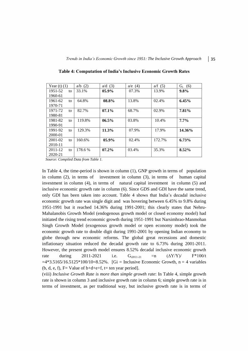
Table 4: Computation of India’s Inclusive Economic Growth Rates

Source: Compiled Data from Table 1.

In Table 4, the time-period is shown in column (1), GNP growth in terms of population

in column (2), in terms of investment in column (3), in terms of human capital

investment in column (4), in terms of natural capital investment in column (5) and

inclusive economic growth rate in column (6). Since GDS and GDI have the same trend,

only GDI has been taken into account. Table 4 shows that India‘s decadal inclusive

economic growth rate was single digit and was hovering between 6.45% to 9.8% during

1951-1991 but it reached 14.36% during 1991-2001; this clearly states that Nehru-

Mahalanobis Growth Model (endogenous growth model or closed economy model) had

initiated the rising trend economic growth during 1951-1991 but Narsimhrao-Manmohan

Singh Growth Model (exogenous growth model or open economy model) took the

economic growth rate to double digit during 1991-2001 by opening Indian economy to

globe through new economic reforms. The global great recessions and domestic

inflationary situation reduced the decadal growth rate to 6.73% during 2001-2011.

However, the present growth model ensures 8.52% decadal inclusive economic growth

rate during 2011-2021 i.e. Gi2011-21 =n (∆Y/Y)/ F*100/t

=4*3.5165/16.5125*100/10=8.52%. [Gi = Inclusive Economic Growth, n = 4 variables

(b, d, e, f), F= Value of b+d+e+f, t= ten year period].

(viii) Inclusive Growth Rate is more than simple growth rate: In Table 4, simple growth

rate is shown in column 3 and inclusive growth rate in column 6; simple growth rate is in

terms of investment, as per traditional way, but inclusive growth rate is in terms of

Year (t) (1) a/b (2) a/d (3) a/e (4) a/f (5) Gi (6)

1951-52 to

1960-61

33.1%

05.9% 07.3%

13.9%

9.8%

1961-62 to

1970-71

64.8%

08.8%

13.8%

02.4%

6.45%

1971-72 to

1980-81

82.7%

07.1%

68.7%

02.9%

7.81%

1981-82 to

1990-91

119.8%

06.5%

03.8%

10.4%

7.7%

1991-92 to

2000-01

129.3%

11.3%

07.9%

17.9%

14.36%

2001-02 to

2010-11

160.6%

05.9%

02.4%

172.7%

6.73%

2011-12 to

2020-21

178.6 %

07.2% 03.4%

35.3% 8.52%

36 PRAGATI: Journal of Indian Economy, Vol. 2, Issue 1

population, investment, human capital and natural capital; hence it is a more appropriate

measurement. In case of India‘s economic growth rate, inclusive growth rate is higher

than simple growth rate but during 1961-91 simple growth rate had declining trend

whereas inclusive growth rate had increasing trend; this means that the simple growth

rate did not represent the growth initiated by declining population growth, increasing

human and natural capital growth which the inclusive growth rate represents.

5.0. Conclusion

It is observed from the analysis that the GNP of India increased from Rs.

105.61 crore in 1951-52 to Rs.71851.59 crore in 2010-11 at 2004-05 prices.

Moreover, when we compute its decadal growth rate, initially it increased from 0.6075

in 1960-61 to 2.8217 in 1990-91 but it declined gradually to 2.6325 in 2010-11. This

means that GNP of India, at 2004-05 prices, increased gradually, and had upward

trend, during 1951-52 to 1990-91; it shows Nehru-Mahalanobis Economic Growth

Model (NMEGM) worked successfully to place Indian economy on growth track. The

period from 1950 to 1980 was crucial for the Indian economy because it witnessed

strong economic policies, programs and measures such as industrial policies, land-

reforms, public sector growth, controlled expansion monetary policies, budgetary

policy, social control, population policy, and export or peril trade policy. However,

GNP decadal growth rate started declining from 1990-91. The post economic reforms

NMSEGM theory of economic growth, initiated during 1990s, attracted more foreign

capital initially but failed to achieve expected growth in agriculture and industrial

sectors; the service sector, no doubt, has raised its share in GNP. Meanwhile, Indian

rupee became cheaper against US dollar, Britain pound sterling and other foreign

currencies. Thus, the GNP decadal growth rate start declining; but when we take

economic growth in terms of population, capital investment, human and natural capital

investment it was higher during 1991-2001 (14.36%). This was because of the

opening of Indian economy, implementation of new economic reforms and service

sector growth in the fields of Information Technology and Bio Technology (ITBT).

The global recession of the first decade of 21th century adversely affected the Indian

economy which lowered the inclusive economic growth during 2001-2011. However,

it recovered to a higher rate (8.52%) during 2011-2021. Moreover, it indicates that

Indian economy has the self-sustaining growth mechanism, initiated by early plans

and development programs that could maintain its growth rate at more than 5%

always, even in adverse conditions.

Trends in India’s Economic Growth since 1951: The Inclusive Growth Approach 37

While measuring economic growth we use model or methods such as G= ∆Y/Y*100

or G= % of gross domestic investment/ capital-output ratio (GDI%/K/O) but there is a

need for including the impact of population, human capital investment and natural

capital development. This study suggests a new method known as ‗inclusive economic

growth method‘ i.e., Gi= n (∆Y/Y)/ F*100/t to compute economic growth rate because it

takes care of both accumulation of wealth by globalised trade and maintenance of

healthy environment for the living-beings on earth.

In conclusion, the economic growth rate measured in the form of change in gross

national product does not give an inclusive picture of the real growth in terms of wealth

accumulation and protection of environment. Increasing productivity through investment

in development of infrastructure, technological up-gradation at the cost of environment

that creates unhealthy atmosphere environmentally, socially, economically and

politically is not economic growth; in true sense, it would be increasing productivity

along with protection and development of natural resources and environment. The

inclusive growth measurement helps to assess the growth in this true sense.

References

Ayres, Robert U. (1998). Turning Point: An End to the Growth Paradigm. London:

Earth Scan Publications. pp. 193–94.

Barro, Robert J. (1997). Determinants of Economic Growth: A Cross-Country Empirical

Study. MIT Press: Cambridge, MA.

Bjork, Gordon J. (1999). The Way it worked and why it won’t: Structural change and

the slowdown of U.S. economic growth. Westport, CT; London: Praeger. pp. 2- 67.

Carlin, Wendy & Soskice, David ( 2006), Macroeconomics: Imperfections, Institutions

& Policies, Oxford University Press.

Domar, Evsey. (1946). Capital expansion, rate of growth and employment.

Econometrica.

Erber, Georg, & Hagemann, Harald. (2002). Growth, structural change, and

employment, In: Frontiers of Economics, ed. Klaus F. Zimmermann, Springer-Verlag,

Berlin – Heidelberg, pp. 269-310: New York.

38 PRAGATI: Journal of Indian Economy, Vol. 2, Issue 1

Feldman, G. A. (1964). On the theory of growth rates of national income. In Spulber,

N. Foundations of Soviet Strategy for Economic Growth. Bloomington: Indiana

University Press.

Foley, Duncan K. (1999). Growth and Distribution Harvard University Press:

Cambridge, MA.

Harrod, Roy F. (1939). An essay in Dynamic theory, Economic Journal 49(March):

14–33.

IMF. (2012). Statistics on the Growth of the Global Gross Domestic Product (GDP)

from 2003 to 2013.

Jones, Charles I. (2002). Introduction to Economic Growth, 2nd ed. W. W. Norton &

Company: New York, N.Y.

Mahalanobis, P. (1953). Some observations on the Process of Growth of National

Income. Sankhya, pp. 307–312.

Romer, Paul. (1994). Beyond Classical and Keynesian Macroeconomic Policy. Policy

Options, 15(July-Aug): 15-21.

Saunders, Harry D. (1992). The Khazzoom-Brookes postulate and neoclassical growth.

The Energy Journal, October.

Schumpeter, Joseph A. (1912). The Theory of Economic Development, 1982 reprint,

Transaction Publishers.

Schumpeter, Joseph A. (1942). Capitalism, Socialism, and Democracy, Harper

Perennial.

Solow, Robert M. (1956). A contribution to the theory of economic growth. Quarterly

Journal of Economics, 70(1): 65-94.

Swan, Trevor W. (1956). Economic growth and capital accumulation. Economic Record,

32: 334–61.

Trends in India’s Economic Growth since 1951: The Inclusive Growth Approach 39

US Department of Energy, Committee on Electricity in Economic Growth Energy

Engineering Board Commission on Engineering and Technical Systems National

Research Council (1986). Electricity in Economic Growth. Washington, DC: National

Academy Press. pp. 16, 40.

Weil, David N. (2008). Economic Growth. 2nd ed. Addison Wesley.

Reports

Planning Commission of India Report (2001). Indian Planning Experience.

Ministry of Environment and Forests Reports (2012-2013).

Reserve Bank of India (2012-13). Handbook of Statistics of Indian Economy.