-

A study of magnetic fields in HII regions usingFaraday rotationCosta, Allison Hainlinehttps://iro.uiowa.edu/discovery/delivery/01IOWA_INST:ResearchRepository/12730606840002771?l#13730726320002771

Costa. (2018). A study of magnetic fields in HII regions using Faraday rotation [University of Iowa].https://doi.org/10.17077/etd.9e5bj65s

Downloaded on 2022/05/28 19:57:46 -0500Copyright © 2018 Allison Hainline CostaFree to read and downloadhttps://iro.uiowa.edu

-

A STUDY OF MAGNETIC FIELDS IN H ii REGIONS USING FARADAYROTATION

by

Allison Hainline Costa

A thesis submitted in partial fulfillment of therequirements for the Doctor of Philosophy

degree in Physics in theGraduate College of The

University of Iowa

May 2018

Thesis Supervisor: Professor Steven Spangler

Copyright by

ALLISON HAINLINE COSTA

2018

All Rights Reserved

Graduate CollegeThe University of Iowa

Iowa City, Iowa

CERTIFICATE OF APPROVAL

PH.D. THESIS

This is to certify that the Ph.D. thesis of

Allison Hainline Costa

has been approved by the Examining Committee for the thesis requirement for theDoctor of Philosophy degree in Physics at the May 2018 graduation.

Thesis Committee:Steven Spangler, Thesis Supervisor

Cornelia Lang

Shea Brown

Kenneth Gayley

Charles Kerton

Robert Mutel

To my husband, Tim, who has given meendless support over the past 10 years.

For my mother, who has alwaysbelieved in me and encouraged me.

For my brother, who has challengedme as only an older brother can.

For my late father, who took me stargazing.

ii

ACKNOWLEDGMENTS

I would like to thank my advisor, Steven Spangler, for his guidance throughout

my career. With his careful mentoring, I have matured as a researcher and writer. I

enjoyed my time as his student immensely.

iii

ABSTRACT

Massive young stars dynamically modify their surroundings, altering their stel-

lar nurseries and the gas that exists between stars. With my research, I assess the

modification of the Galactic magnetic field within H ii regions and stellar bubbles

associated with OB stars. Because H ii regions are plasmas, magnetic fields should

be important to the dynamics of the region. Understanding how the magnetic field

is modified in these structures is critical for inputs to simulations and for assessing

stellar feedback. To obtain information on the properties of the magnetic field, I

measure the Faraday rotation of linearly polarized radio waves that pass through the

plasma of the H ii region.

In this thesis, I present results of Faraday rotation studies of two Galactic H ii

regions. The first is the Rosette Nebula (l = 206, b = -1.2), and the second is IC

1805 (l = 135, b = 0.9), which is associated with the W4 Superbubble. I measure

positive rotation measure (RM) values in excess of +40 to +1200 rad m−2 due to

the shell of the Rosette nebula and a background RM of +147 rad m−2 due to the

general interstellar medium in this area of the Galactic plane. In the area of IC 1805,

I measure negative RM values between +600 and –800 rad m−2 due to the H ii region.

The sign of the RM across each H ii region is consistent with the expected polarity

of the large-scale Galactic magnetic field that follows the Perseus spiral arm in the

clockwise direction, as suggested by Van Eck et al. (2011, ApJ, 728, 14).

I find that the Rosette Nebula and IC 1805 constitute a “Faraday rotation

anomaly”, or a region of increased RM relative to the general Galactic background

value. Although the RM observed on lines of sight through the region vary substan-

tially, the |RM| due to the nebula is commonly 100 – 1000 rad m−2. In spite of this,

iv

the observed RMs are not as large as simple, analytic models of magnetic field am-

plification in H ii regions (such as by magnetic flux conservation in a swept-up shell)

might indicate. This suggests that the Galactic field is not increased by a substantial

factor within the ionized gas in an H ii region. Finally, these results show intrigu-

ing indications that some of the largest values of |RM| occur for lines of sight that

pass outside the fully ionized shell of the IC 1805 H ii region, but pass through the

Photodissociation Region (PDR) associated with IC 1805.

v

PUBLIC ABSTRACT

Massive young stars dynamically modify their surroundings, altering their stel-

lar nurseries and the gas that exists between stars. These massive stars create regions

of ions and free electrons (plasmas) in which the magnetic field is “frozen”, so mag-

netic fields should be important to the dynamics of these regions. Magnetic fields

may provide support against gravity, which would suppress future star formation in

the region, or magnetic fields may suppress turbulence, which would encourage star

formation.

With my research, I investigate how the Galactic magnetic field is modified in

these regions with respect to the ambient (external) medium. In this work, I present

results of a study of two regions in the Milky Way where massive stars have modified

their surrounding. The stars are relatively young and nearby in the Perseus Arm

of the galaxy. From my analyses, it appears that the Galactic magnetic field is not

sensitive to the presence of these regions because the magnitude and the direction of

the magnetic field is not modified due to the plasma in these two regions.

vi

TABLE OF CONTENTS

LIST OF TABLES . . . . . . . . . . . . . . . . . . . . . . . . . . . . . . . . . x

LIST OF FIGURES . . . . . . . . . . . . . . . . . . . . . . . . . . . . . . . . xii

CHAPTER

1 Introduction to Thesis Research . . . . . . . . . . . . . . . . . . . . . 1

1.1 Introduction . . . . . . . . . . . . . . . . . . . . . . . . . . . . . 11.2 Faraday Rotation as a Measurement of Magnetic Fields . . . . . 21.3 Previous Results of Importance . . . . . . . . . . . . . . . . . . . 31.4 Outline of Thesis . . . . . . . . . . . . . . . . . . . . . . . . . . . 4

2 Denser Sampling of the Rosette Nebula with Faraday Rotation Mea-surements: Improved Estimates of Magnetic Fields in H ii Regions . . 6

2.1 Introduction . . . . . . . . . . . . . . . . . . . . . . . . . . . . . 62.1.1 Previous Results on Faraday Rotation through H ii Regions 8

2.2 Observations . . . . . . . . . . . . . . . . . . . . . . . . . . . . . 112.3 Data Reduction . . . . . . . . . . . . . . . . . . . . . . . . . . . 12

2.3.1 Determination of Rotation Measures Using Two Techniques 162.4 Observational Results . . . . . . . . . . . . . . . . . . . . . . . . 22

2.4.1 Comparison of Techniques for RM Measurement . . . . . 252.5 Diagnostics of Magnetic Fields in H ii Regions Utilizing Plasma

Shell Models . . . . . . . . . . . . . . . . . . . . . . . . . . . . . 262.5.1 Empirical Models for Stellar Bubbles . . . . . . . . . . . . 262.5.2 A Bayesian Statistical Approach to Compare Shell Models

and Determine the Orientation of the Interstellar MagneticField . . . . . . . . . . . . . . . . . . . . . . . . . . . . . 32

2.5.3 Simplified Inhomogeneous Shell Models . . . . . . . . . . 382.5.4 Summary of Bayesian Test of Models . . . . . . . . . . . 50

2.6 Summary and Conclusions . . . . . . . . . . . . . . . . . . . . . 52

3 A Faraday Rotation Study of the Stellar Bubble and H ii Region Asso-ciated with the W4 Complex . . . . . . . . . . . . . . . . . . . . . . . 55

3.1 Introduction . . . . . . . . . . . . . . . . . . . . . . . . . . . . . 553.1.1 Techniques for Measuring Magnetic Fields in the Interstel-

lar Medium . . . . . . . . . . . . . . . . . . . . . . . . . . 563.1.2 The H ii Region and Stellar Bubble Associated with the

W4 Complex . . . . . . . . . . . . . . . . . . . . . . . . . 56

vii

3.2 Observations . . . . . . . . . . . . . . . . . . . . . . . . . . . . . 643.2.1 Source Selection . . . . . . . . . . . . . . . . . . . . . . . 643.2.2 VLA Observations . . . . . . . . . . . . . . . . . . . . . . 67

3.3 Data Reduction . . . . . . . . . . . . . . . . . . . . . . . . . . . 693.3.1 Rotation Measure Analysis via a Least-Squares Fit to χ vs

λ2 . . . . . . . . . . . . . . . . . . . . . . . . . . . . . . 703.3.2 Rotation Measure Synthesis . . . . . . . . . . . . . . . . 72

3.4 Observational Results . . . . . . . . . . . . . . . . . . . . . . . . 763.4.1 Measurements of Radio Sources Viewed Through the W4

Complex . . . . . . . . . . . . . . . . . . . . . . . . . . . 763.4.2 Report on Faraday Complexity and Unpolarized Lines of

Sight . . . . . . . . . . . . . . . . . . . . . . . . . . . . . 783.4.3 A Unique Line of Sight Through the W4 Region: LSI

+61303 . . . . . . . . . . . . . . . . . . . . . . . . . . . 813.5 Results on Faraday Rotation Through the W4 Complex . . . . . 84

3.5.1 The Rotation Measure Sky in the Direction of W4 . . . . 843.5.2 The Galactic Background RM in the Direction of W4 . . 853.5.3 High Faraday Rotation Through Photodissociation Regions 873.5.4 Faraday Rotation Through the Cavity and Shell of the Stel-

lar Bubble . . . . . . . . . . . . . . . . . . . . . . . . . . 913.5.5 Low Rotation Measure Values Through the W4 Superbubble 92

3.6 Models for the Structure of the H ii region and Stellar Bubble . . 943.6.1 Whiting et al. (2009) Model of the Rotation Measure in

the Shell of a Magnetized Bubble . . . . . . . . . . . . . . 943.6.2 Analytical Approximation to Magnetized Bubbles of Ferriere

et al. (1991) . . . . . . . . . . . . . . . . . . . . . . . . . 973.7 Discussion of Observational Results . . . . . . . . . . . . . . . . 106

3.7.1 Comparison of Models with Observations in the H ii Region 1063.7.2 Magnetic Fields in the PDR . . . . . . . . . . . . . . . . 108

3.8 A Comparison of IC 1805 and the Rosette Nebula as “RotationMeasure Anomalies” . . . . . . . . . . . . . . . . . . . . . . . . 110

3.9 Future Research . . . . . . . . . . . . . . . . . . . . . . . . . . . 1123.10 Summary and Conclusions . . . . . . . . . . . . . . . . . . . . . 113

4 Supporting Work . . . . . . . . . . . . . . . . . . . . . . . . . . . . . 116

4.1 Analysis of Spectral Indices for Radio Sources . . . . . . . . . . . 1164.2 Faraday Complex Sources . . . . . . . . . . . . . . . . . . . . . . 119

4.2.1 Introduction . . . . . . . . . . . . . . . . . . . . . . . . . 1194.2.2 Depolarization Models . . . . . . . . . . . . . . . . . . . . 1234.2.3 Results of the QU Analysis . . . . . . . . . . . . . . . . . 126

4.3 Photodissociation Regions . . . . . . . . . . . . . . . . . . . . . . 1304.4 Assessing Faraday Rotation and Nebular Properties from the Lit-

erature . . . . . . . . . . . . . . . . . . . . . . . . . . . . . . . . 134

viii

5 Summary . . . . . . . . . . . . . . . . . . . . . . . . . . . . . . . . . . 139

6 Future Research . . . . . . . . . . . . . . . . . . . . . . . . . . . . . . 142

6.1 Modification of the Galactic Magnetic Field near IC 1396 . . . . 1426.2 Compact H ii Regions at ` ∼ 328 . . . . . . . . . . . . . . . . . 1436.3 Faraday complex Sources Using Simulated Data . . . . . . . . . 143

APPENDIX

A CASA Maps for Lines of Sight Through or Near to IC 1805 . . . . . . 144

B Figures for RM Synthesis Analysis . . . . . . . . . . . . . . . . . . . . 152

C Figures and Tables for QU Analysis . . . . . . . . . . . . . . . . . . . 160

BIBLIOGRAPHY . . . . . . . . . . . . . . . . . . . . . . . . . . . . . . . . . 175

ix

LIST OF TABLES

2.1 Log of Observations . . . . . . . . . . . . . . . . . . . . . . . . . . . . . 13

2.2 List of Sources Observed . . . . . . . . . . . . . . . . . . . . . . . . . . . 13

2.3 New Faraday Rotation Measurements through the Rosette Nebula . . . . 24

2.4 Input Parameters for Shell Models . . . . . . . . . . . . . . . . . . . . . 30

2.5 Results of Bayesian Analysis . . . . . . . . . . . . . . . . . . . . . . . . . 37

2.6 Local Parameters for Lines of Sight Through the Shell . . . . . . . . . . . 39

2.7 Results of Filling Factor . . . . . . . . . . . . . . . . . . . . . . . . . . . 48

3.1 List of Sources Observed . . . . . . . . . . . . . . . . . . . . . . . . . . . 66

3.2 Log of Observations . . . . . . . . . . . . . . . . . . . . . . . . . . . . . 67

3.3 Rotation Measure Synthesis Parameters . . . . . . . . . . . . . . . . . . . 73

3.4 Faraday Rotation Measurement Values through the W4 Complex . . . . 77

3.5 List of Sources with RM values from Catalogs . . . . . . . . . . . . . . . 86

3.6 Model Parameters . . . . . . . . . . . . . . . . . . . . . . . . . . . . . . 96

3.7 Stellar Parameters . . . . . . . . . . . . . . . . . . . . . . . . . . . . . . 111

4.1 Flux Densities for Lines of Sight through IC 1805 . . . . . . . . . . . . . 117

4.2 Flux Densities for Lines of Sight Through the Rosette Nebula . . . . . . 118

4.3 H ii Regions From Literature . . . . . . . . . . . . . . . . . . . . . . . . . 136

4.4 Comparison of Wind Luminosities and RMs for H ii Regions . . . . . . . 137

C.1 Results of QU Analysis for 4 MHz “Fractional” Data . . . . . . . . . . . 161

C.2 Results of QU Analysis for 4 MHz “Corrected” Data . . . . . . . . . . . . 162

x

C.3 Results of QU Analysis for 128 MHz Data . . . . . . . . . . . . . . . . . 163

C.4 Results of QU Analysis for 128 MHz Data Cont. . . . . . . . . . . . . . . 164

xi

LIST OF FIGURES

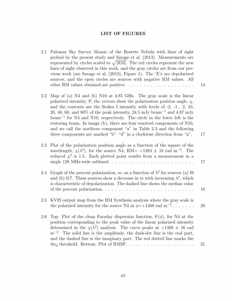
2.1 Palomar Sky Survey Mosaic of the Rosette Nebula with lines of sightprobed by the present study and Savage et al. (2013). Measurements arerepresented by circles scaled to

√|RM|. The red circles represent the new

lines of sight observed in this work, and the gray circles are from our pre-vious work (see Savage et al. (2013), Figure 1). The ‘X’s are depolarizedsources, and the open circles are sources with negative RM values. Allother RM values obtained are positive. . . . . . . . . . . . . . . . . . . . 14

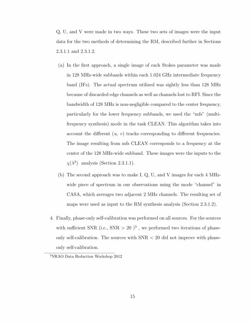
2.2 Map of (a) N4 and (b) N10 at 4.85 GHz. The gray scale is the linearpolarized intensity, P, the vectors show the polarization position angle, χ,and the contours are the Stokes I intensity with levels of -2, -1 , 2, 10,20, 40, 60, and 80% of the peak intensity, 24.5 mJy beam−1 and 4.87 mJybeam−1 for N4 and N10, respectively. The circle in the lower left is therestoring beam. In image (b), there are four resolved components of N10,and we call the northern component “a” in Table 2.3 and the followingthree components are marked “b”–“d” in a clockwise direction from “a”. 17

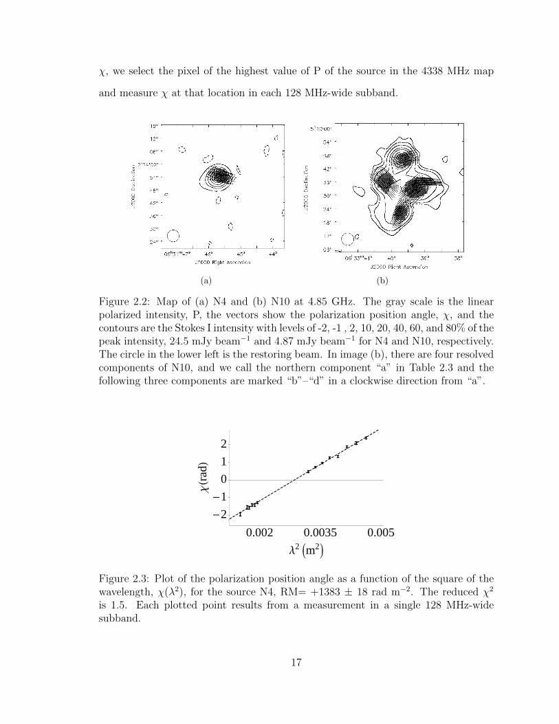
2.3 Plot of the polarization position angle as a function of the square of thewavelength, χ(λ2), for the source N4, RM= +1383 ± 18 rad m−2. Thereduced χ2 is 1.5. Each plotted point results from a measurement in asingle 128 MHz-wide subband. . . . . . . . . . . . . . . . . . . . . . . . . 17

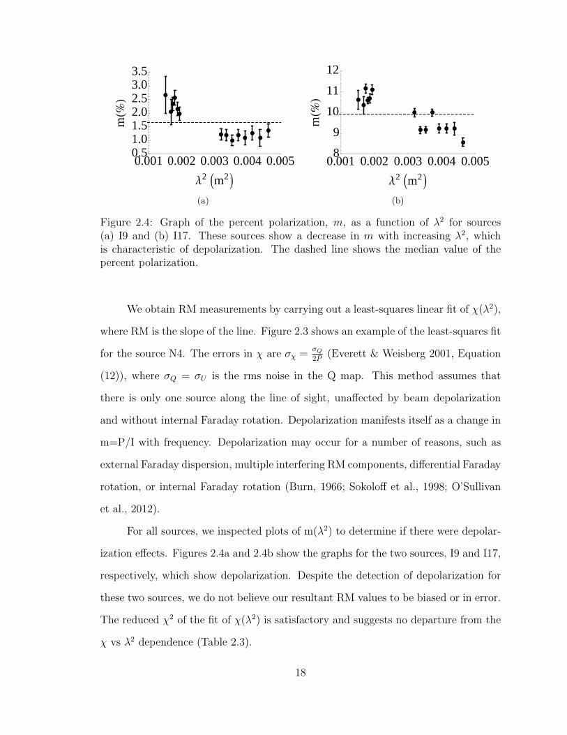
2.4 Graph of the percent polarization, m, as a function of λ2 for sources (a) I9and (b) I17. These sources show a decrease in m with increasing λ2, whichis characteristic of depolarization. The dashed line shows the median valueof the percent polarization. . . . . . . . . . . . . . . . . . . . . . . . . . . 18

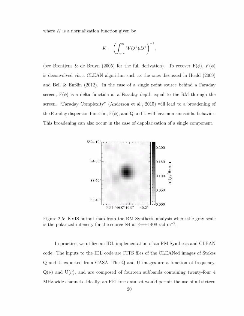
2.5 KVIS output map from the RM Synthesis analysis where the gray scale isthe polarized intensity for the source N4 at φ=+1408 rad m−2. . . . . . . 20

2.6 Top: Plot of the clean Faraday dispersion function, F(φ), for N4 at theposition corresponding to the peak value of the linear polarized intensitydetermined in the χ(λ2) analysis. The curve peaks at +1408 ± 16 radm−2. The solid line is the amplitude, the dash-dot line is the real part,and the dashed line is the imaginary part. The red dotted line marks the3σQ threshold. Bottom: Plot of RMSF. . . . . . . . . . . . . . . . . . . . 21

xii

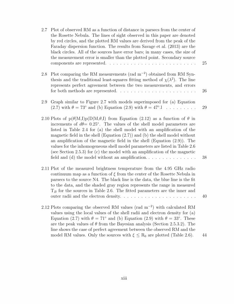
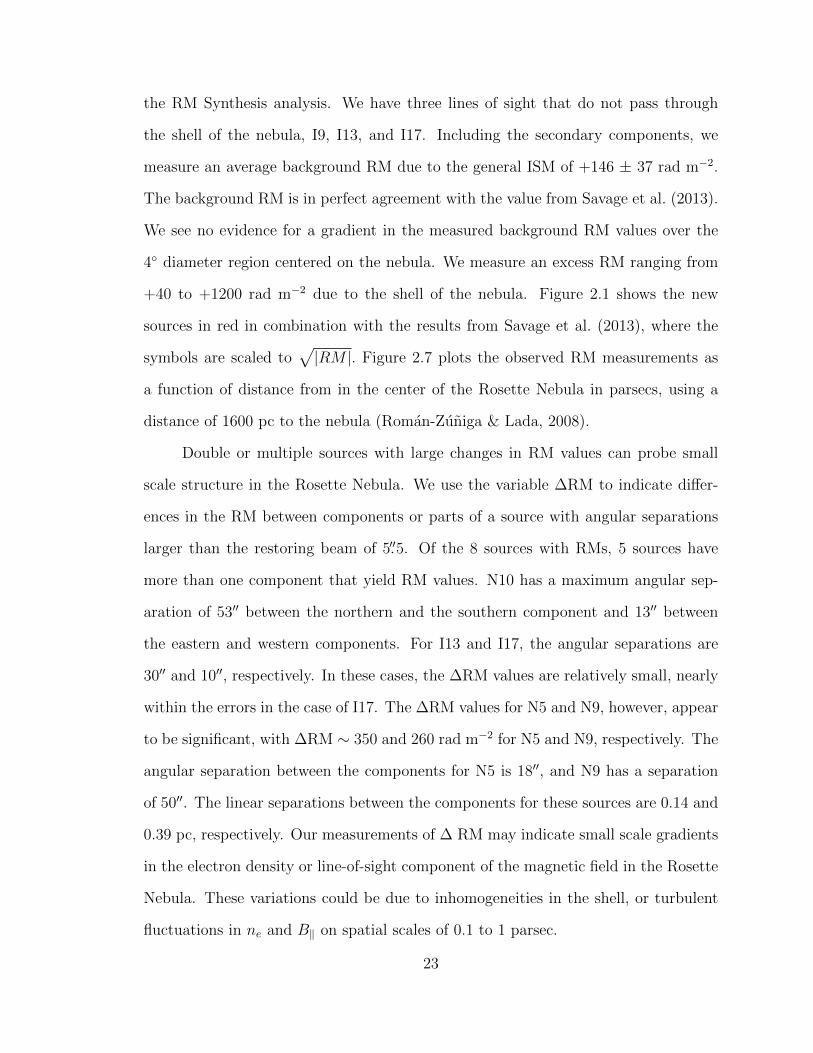
2.7 Plot of observed RM as a function of distance in parsecs from the center ofthe Rosette Nebula. The lines of sight observed in this paper are denotedby red circles, and the plotted RM values are derived from the peak of theFaraday dispersion function. The results from Savage et al. (2013) are theblack circles. All of the sources have error bars; in many cases, the size ofthe measurement error is smaller than the plotted point. Secondary sourcecomponents are represented. . . . . . . . . . . . . . . . . . . . . . . . . . 25

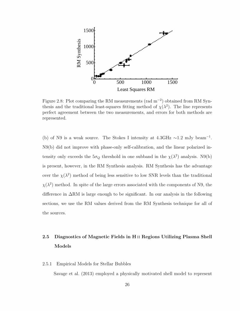
2.8 Plot comparing the RM measurements (rad m−2) obtained from RM Syn-thesis and the traditional least-squares fitting method of χ(λ2). The linerepresents perfect agreement between the two measurements, and errorsfor both methods are represented. . . . . . . . . . . . . . . . . . . . . . . 26

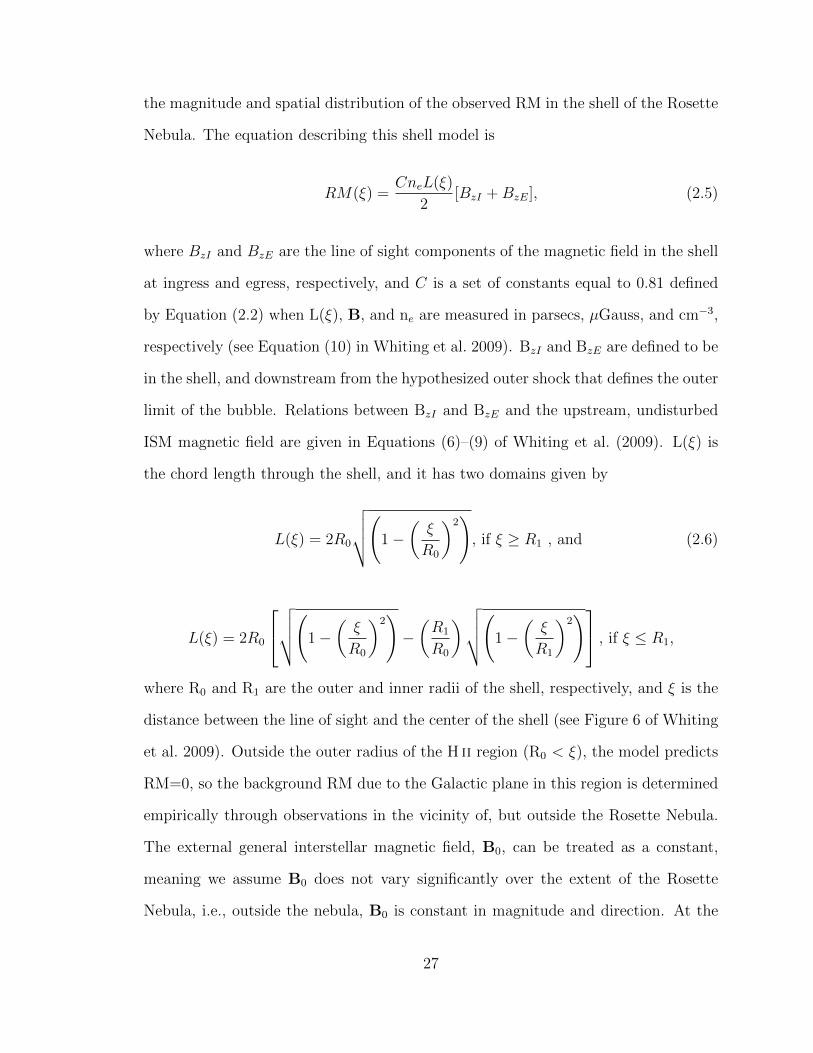
2.9 Graph similar to Figure 2.7 with models superimposed for (a) Equation(2.7) with θ = 73 and (b) Equation (2.9) with θ = 47.l . . . . . . . . . 29

2.10 Plots of p(θ|M,I)p(D|M,θ,I) from Equation (2.12) as a function of θ inincrements of dθ= 0.25. The values of the shell model parameters arelisted in Table 2.4 for (a) the shell model with an amplification of themagnetic field in the shell (Equation (2.7)) and (b) the shell model withoutan amplification of the magnetic field in the shell (Equation (2.9)). Thevalues for the inhomogeneous shell model parameters are listed in Table 2.6(see Section 2.5.3) for (c) the model with an amplification of the magneticfield and (d) the model without an amplification. . . . . . . . . . . . . . . 38

2.11 Plot of the measured brightness temperature from the 4.95 GHz radiocontinuum map as a function of ξ from the center of the Rosette Nebula inparsecs to the source N4. The black line is the data, the blue line is the fitto the data, and the shaded gray region represents the range in measuredTB for the sources in Table 2.6. The fitted parameters are the inner andouter radii and the electron density. . . . . . . . . . . . . . . . . . . . . . 40

2.12 Plots comparing the observed RM values (rad m−2) with calculated RMvalues using the local values of the shell radii and electron density for (a)Equation (2.7) with θ = 71 and (b) Equation (2.9) with θ = 33. Theseare the peak values of θ from the Bayesian analysis (Section 2.5.3.2). Theline shows the case of perfect agreement between the observed RM and themodel RM values. Only the sources with ξ ≤ R0 are plotted (Table 2.6). 44

xiii

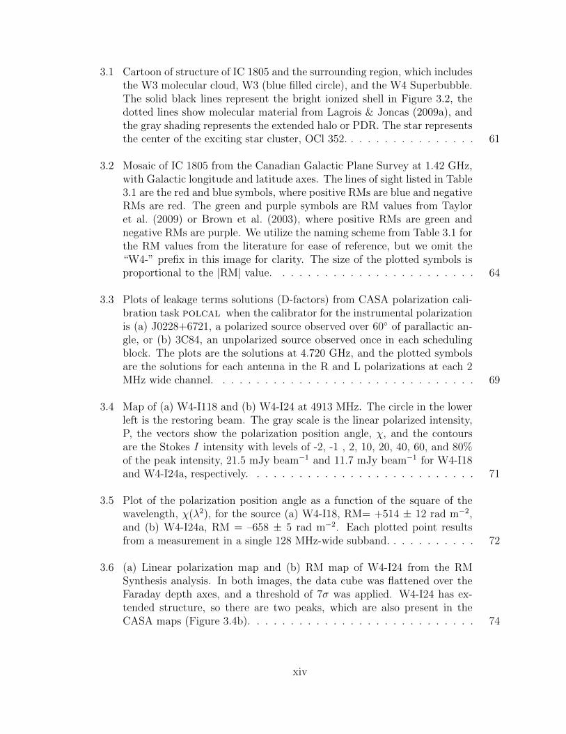
3.1 Cartoon of structure of IC 1805 and the surrounding region, which includesthe W3 molecular cloud, W3 (blue filled circle), and the W4 Superbubble.The solid black lines represent the bright ionized shell in Figure 3.2, thedotted lines show molecular material from Lagrois & Joncas (2009a), andthe gray shading represents the extended halo or PDR. The star representsthe center of the exciting star cluster, OCl 352. . . . . . . . . . . . . . . . 61

3.2 Mosaic of IC 1805 from the Canadian Galactic Plane Survey at 1.42 GHz,with Galactic longitude and latitude axes. The lines of sight listed in Table3.1 are the red and blue symbols, where positive RMs are blue and negativeRMs are red. The green and purple symbols are RM values from Tayloret al. (2009) or Brown et al. (2003), where positive RMs are green andnegative RMs are purple. We utilize the naming scheme from Table 3.1 forthe RM values from the literature for ease of reference, but we omit the“W4-” prefix in this image for clarity. The size of the plotted symbols isproportional to the |RM| value. . . . . . . . . . . . . . . . . . . . . . . . 64

3.3 Plots of leakage terms solutions (D-factors) from CASA polarization cali-bration task polcal when the calibrator for the instrumental polarizationis (a) J0228+6721, a polarized source observed over 60 of parallactic an-gle, or (b) 3C84, an unpolarized source observed once in each schedulingblock. The plots are the solutions at 4.720 GHz, and the plotted symbolsare the solutions for each antenna in the R and L polarizations at each 2MHz wide channel. . . . . . . . . . . . . . . . . . . . . . . . . . . . . . . 69

3.4 Map of (a) W4-I118 and (b) W4-I24 at 4913 MHz. The circle in the lowerleft is the restoring beam. The gray scale is the linear polarized intensity,P, the vectors show the polarization position angle, χ, and the contoursare the Stokes I intensity with levels of -2, -1 , 2, 10, 20, 40, 60, and 80%of the peak intensity, 21.5 mJy beam−1 and 11.7 mJy beam−1 for W4-I18and W4-I24a, respectively. . . . . . . . . . . . . . . . . . . . . . . . . . . 71

3.5 Plot of the polarization position angle as a function of the square of thewavelength, χ(λ2), for the source (a) W4-I18, RM= +514 ± 12 rad m−2,and (b) W4-I24a, RM = –658 ± 5 rad m−2. Each plotted point resultsfrom a measurement in a single 128 MHz-wide subband. . . . . . . . . . . 72

3.6 (a) Linear polarization map and (b) RM map of W4-I24 from the RMSynthesis analysis. In both images, the data cube was flattened over theFaraday depth axes, and a threshold of 7σ was applied. W4-I24 has ex-tended structure, so there are two peaks, which are also present in theCASA maps (Figure 3.4b). . . . . . . . . . . . . . . . . . . . . . . . . . . 74

xiv

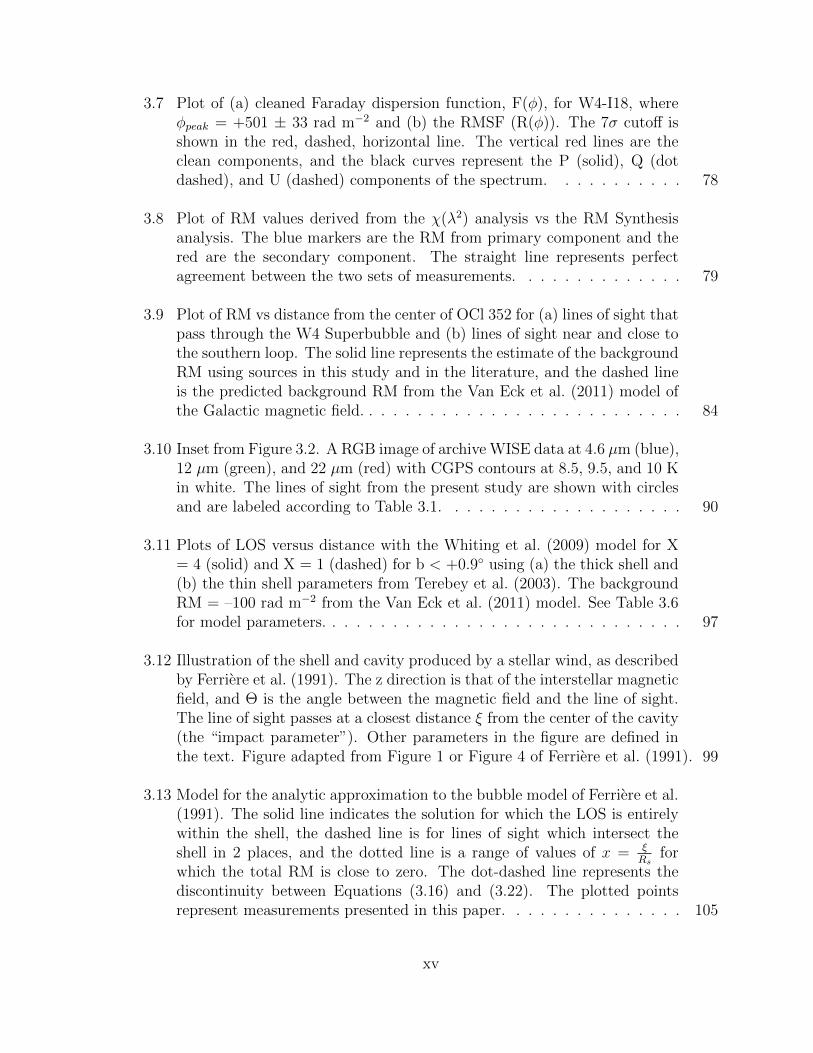
3.7 Plot of (a) cleaned Faraday dispersion function, F(φ), for W4-I18, whereφpeak = +501 ± 33 rad m−2 and (b) the RMSF (R(φ)). The 7σ cutoff isshown in the red, dashed, horizontal line. The vertical red lines are theclean components, and the black curves represent the P (solid), Q (dotdashed), and U (dashed) components of the spectrum. . . . . . . . . . . 78

3.8 Plot of RM values derived from the χ(λ2) analysis vs the RM Synthesisanalysis. The blue markers are the RM from primary component and thered are the secondary component. The straight line represents perfectagreement between the two sets of measurements. . . . . . . . . . . . . . 79

3.9 Plot of RM vs distance from the center of OCl 352 for (a) lines of sight thatpass through the W4 Superbubble and (b) lines of sight near and close tothe southern loop. The solid line represents the estimate of the backgroundRM using sources in this study and in the literature, and the dashed lineis the predicted background RM from the Van Eck et al. (2011) model ofthe Galactic magnetic field. . . . . . . . . . . . . . . . . . . . . . . . . . . 84

3.10 Inset from Figure 3.2. A RGB image of archive WISE data at 4.6 µm (blue),12 µm (green), and 22 µm (red) with CGPS contours at 8.5, 9.5, and 10 Kin white. The lines of sight from the present study are shown with circlesand are labeled according to Table 3.1. . . . . . . . . . . . . . . . . . . . 90

3.11 Plots of LOS versus distance with the Whiting et al. (2009) model for X= 4 (solid) and X = 1 (dashed) for b < +0.9 using (a) the thick shell and(b) the thin shell parameters from Terebey et al. (2003). The backgroundRM = –100 rad m−2 from the Van Eck et al. (2011) model. See Table 3.6for model parameters. . . . . . . . . . . . . . . . . . . . . . . . . . . . . . 97

3.12 Illustration of the shell and cavity produced by a stellar wind, as describedby Ferriere et al. (1991). The z direction is that of the interstellar magneticfield, and Θ is the angle between the magnetic field and the line of sight.The line of sight passes at a closest distance ξ from the center of the cavity(the “impact parameter”). Other parameters in the figure are defined inthe text. Figure adapted from Figure 1 or Figure 4 of Ferriere et al. (1991). 99

3.13 Model for the analytic approximation to the bubble model of Ferriere et al.(1991). The solid line indicates the solution for which the LOS is entirelywithin the shell, the dashed line is for lines of sight which intersect theshell in 2 places, and the dotted line is a range of values of x = ξ

Rsfor

which the total RM is close to zero. The dot-dashed line represents thediscontinuity between Equations (3.16) and (3.22). The plotted pointsrepresent measurements presented in this paper. . . . . . . . . . . . . . . 105

xv

4.1 Histogram of spectral indices for sources in Tables 4.1 and 4.2 . . . . . . 119

4.2 Plot Sν vs ν for (a) W4-I8, (b) W4-I12, (c) W4-O4, (d) R-N4, (e) R-N7,and (f) R-N10L. These sources have a significant (> 7σQU) peak in F (φ). 120

4.3 Comparison of RM Synthesis results to least-squares fit method for theRM. The results from the Rosette Nebula are shown in blue and in redfor IC 1805. The solid line represents perfect agreement between the twomeasurements. . . . . . . . . . . . . . . . . . . . . . . . . . . . . . . . . . 121

4.4 Cartoon of depolarization models including (a) Faraday thin, (b) externalFaraday dispersion/ beam depolarization, (c) differential Faraday rotation,and (d) internal Faraday dispersion. In each case, the blue region repre-sents a magnetized medium that has thermal electrons. The ‘source’ isnon-thermal emission, and when the source is the blue medium, the mate-rial is both emitting and rotating the emission. . . . . . . . . . . . . . . . 125

4.5 Plots of Q vs U of the corrected data for (a) W4-I24a and (b) W4-I1. Thecolor of the symbols indicates the value of λ2 associated with the Q and Udata where blue, is the short wavelengths and red is the long wavelengths. 129

4.6 RGB image of archive WISE data at 4.6 µm (blue), 12 µm (green), and 22µm (red) with radio continuum contours from CGPS in white. The lines ofsight from the present study are shown with circles and are labeled similarto Figure 3.2. . . . . . . . . . . . . . . . . . . . . . . . . . . . . . . . . . 132

4.7 RGB image of WISE data at 4.6 µm (blue), 12 µm (green), and 22 µm (red)with radio continuum contours at 4.5 GHz (see Celnik 1985) at 4 and 6times the background signal in white. The lines of sight from the presentstudy are shown with circles and are labeled similar to Figure 5.1b. . . . 133

4.8 (a) Plot of RM values vs wind luminosity of the principle ionizing star ineach H ii region. The ranges of the RM values are given in Table 4.4. TheH ii regions that do not have an estimate of Lw are not shown. (b) Plot ofRM vs diameter and (c) RM vs electron density. The inset plot includesNGC 6334A. . . . . . . . . . . . . . . . . . . . . . . . . . . . . . . . . . . 138

5.1 (a) Radio continuum mosaic of IC 1805 at 1.42 GHz from the CGPS. Theaxes are in Galactic coordinates, and the white “x” represents the centerof the star cluster associated with the nebula. (b) Palomar Sky Surveymosaic of the Rosette Nebula similar to Figure 1 of Costa et al. (2016). . 139

xvi

6.1 Palomar Sky Survey mosaic of IC 1396 with observed lines of sights rep-resented by filled circles. The blue circles represent lines of sight observedto probe the background RM, and the red are through the ionized shell.The three parallel lines in the lower right corner are image artifacts. . . . 142

A.1 CASA Maps for W4-I1, -I2, -I3, and -I4. . . . . . . . . . . . . . . . . . . 145

A.2 CASA Maps for W4-I6, -I8, -I11, and -I12. . . . . . . . . . . . . . . . . . 146

A.3 CASA Maps for W4-I13, -I14, I15, and -I16. . . . . . . . . . . . . . . . . 147

A.4 CASA Maps for W4-I17, -I18, -I19, and -I20. . . . . . . . . . . . . . . . . 148

A.5 CASA Maps for W4-I21, -I23, -I24, and -O1. . . . . . . . . . . . . . . . 149

A.6 CASA Maps for W4-O2, -O4, -O5, and -O6. . . . . . . . . . . . . . . . . 150

A.7 CASA Maps for W4-O7, -O8, and -O10. . . . . . . . . . . . . . . . . . . 151

B.1 RM Synthesis Results for sources W4-I1, -I2, -I2b, -I3, -I4, -I4b, -I6, and -I8.153

B.2 RM Synthesis Results for sources W4-I11, -I12, -I13, -I13b, -I14, -I14b,-I15, and -I17. . . . . . . . . . . . . . . . . . . . . . . . . . . . . . . . . . 154

B.3 RM Synthesis Results for sources W4-I17b, -I18, -I19, -I21, -I21b, -I21c,-I23, and -I23b. . . . . . . . . . . . . . . . . . . . . . . . . . . . . . . . . 155

B.4 RM Synthesis Results for sources W4-I23c, -I24, -O1, -O2, -O4, -O5, -O6,and -O7. . . . . . . . . . . . . . . . . . . . . . . . . . . . . . . . . . . . . 156

B.5 RM Synthesis Results for sources W4-O8, W4-O10, R-I9, R-I13, R-I13b,-I17, -I17b, and -N4. . . . . . . . . . . . . . . . . . . . . . . . . . . . . . 157

B.6 RM Synthesis Results for sources R-N5, -N5b, -N7, -N9, -N9b, -N10T,-N10R, and -N10B. . . . . . . . . . . . . . . . . . . . . . . . . . . . . . . 158

B.7 RM Synthesis Results for sources R-N10L. . . . . . . . . . . . . . . . . . 159

C.1 Representative Triangular Confidence Plot for a 2 Faraday Thin Model. . 165

C.2 Representative Best Fit Parameters for 2 Faraday Thin. . . . . . . . . . . 166

C.3 Representative Triangular Confidence Plot for a 2 EFD+2 Faraday ThinModel. . . . . . . . . . . . . . . . . . . . . . . . . . . . . . . . . . . . . . 167

xvii

C.4 Representative Best Fit Parameters for a 2 EFD+2 Faraday Thin. . . . . 168

C.5 Representative Triangular Confidence Plot for a Uniform Slab+FaradayThin Model. . . . . . . . . . . . . . . . . . . . . . . . . . . . . . . . . . . 169

C.6 Representative Best Fit Parameters for a Uniform Slab+Faraday Thin Model.170

C.7 Representative Triangular Confidence Plot for an EFD Model. . . . . . . 171

C.8 Representative Best Fit Parameters for an EFD Model. . . . . . . . . . . 172

C.9 Representative Triangular Confidence Plot for a 2 Faraday Thin+ EFDModel for 128 MHz Data. . . . . . . . . . . . . . . . . . . . . . . . . . . . 173

C.10 Representative Best Fit Parameters for 2 Faraday Thin+ EFD Model for128 MHz Data. . . . . . . . . . . . . . . . . . . . . . . . . . . . . . . . . 174

xviii

CHAPTER 1

INTRODUCTION TO THESIS RESEARCH

1.1 Introduction

OB associations energize the interstellar medium (ISM) via their stellar winds

and by photoionizing the surrounding gas. In doing so, they modify the material in

the ISM and interact with the pervasive Galactic magnetic field, which is locked into

the ISM plasma. While shocks from stellar winds and ionization fronts may quench

or trigger star formation in the region, it is necessary to also include magnetic fields

in stellar feedback models. Models that include magnetic field information suggest

that magnetic pressure may provide support against gravitational collapse (Passot

et al., 1995; Kortgen & Banerjee, 2015); however, recent simulations by Zamora-

Aviles et al. (2018) suggest that magnetic fields can suppress turbulence, which then

promotes star formation. Observations of magnetic field properties in regions of recent

star formation provide constraints on stellar feedback simulations and on models to

understand magnetic fields in star forming environments.

Magnetic fields should have a direct impact on the growth of stellar bubbles

and H ii regions, as well as the future star formation in the region. Magnetic fields

are frozen into the plasma of the H ii region, and the stellar winds of the star can

transport magnetic field lines out into the ISM. The simple case of radial expansion of

the stellar wind and H ii region is modified by the presence of the swept up magnetic

field lines. The shells of magnetized bubbles can be elongated in the direction of the

field lines as well as thicken the shells of the bubbles (Ferriere et al., 1991).

With my research, I assess how the Galactic magnetic field is modified near

OB associations by probing the magnetic field within the shells of H ii regions, wind-

blown bubbles, and peripheries of the H ii regions. By determining the orientation

1

and magnitude of the magnetic field in these dynamic structures, I investigate links

between the properties of the magnetic field and the environment, such as star for-

mation activity, structure of the H ii region, and the wind luminosity of the stars

responsible for the H ii region.

As part of this work, I am developing techniques to identify and interpret mag-

netic field information along complex lines of sight that may, for example, contain

multiple media with turbulent magnetic fields. This work is important to studies of

magnetic fields in other environments such as the solar corona, and the analyses and

discussions in this work are applicable to magnetic fields in extragalactic environments

as well.

With my research, I attempt to answer the following questions. 1) How is the

Galactic magnetic field altered, in either magnitude or direction, due to the presence of

wind-blown bubbles and H ii regions? 2) To what extent is the modification dependent

on properties of the exciting star cluster (e.g., stellar content, wind luminosity, extent

of the bubble)? To answer these questions, I have undertaken observing projects of

two Galactic H ii regions with the NSF’s Karl G. Jansky Very Large Array (VLA).

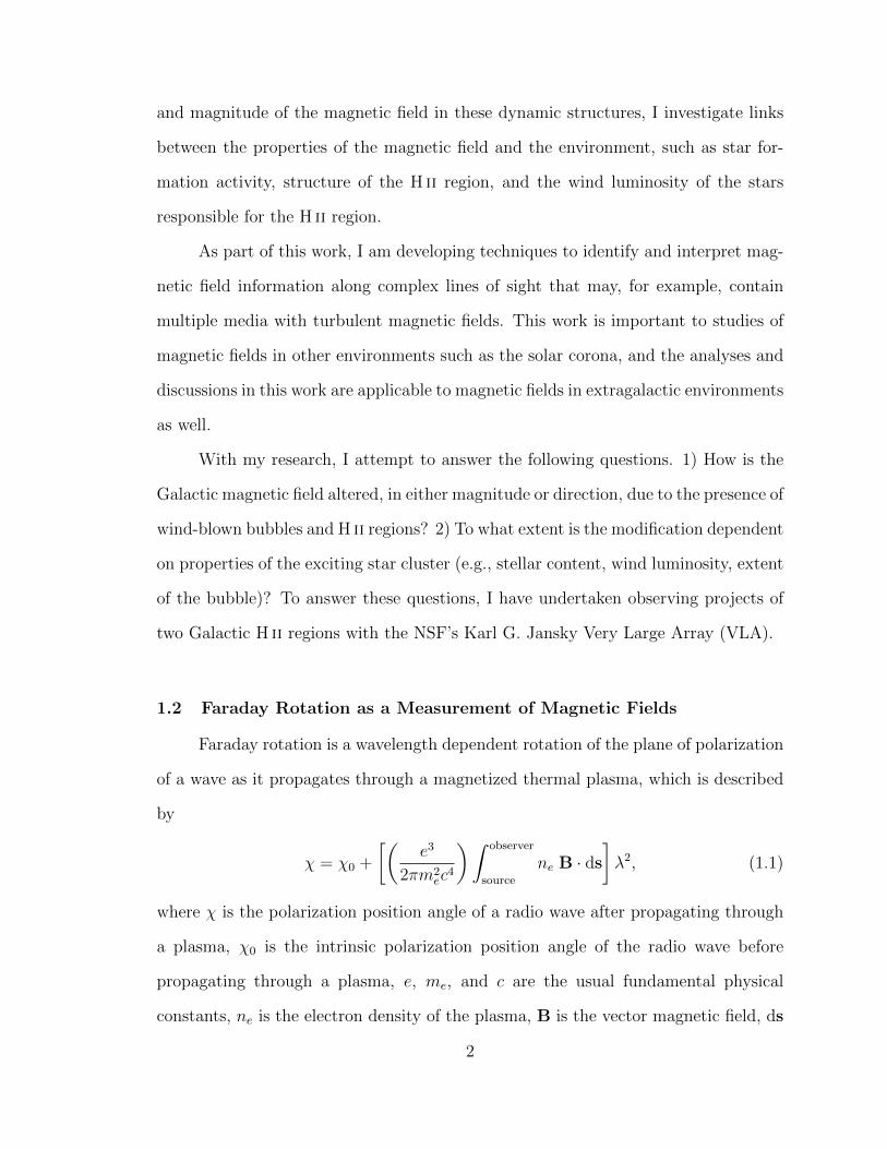
1.2 Faraday Rotation as a Measurement of Magnetic Fields

Faraday rotation is a wavelength dependent rotation of the plane of polarization

of a wave as it propagates through a magnetized thermal plasma, which is described

by

χ = χ0 +

[(e3

2πm2ec

4

)∫ observer

source

ne B · ds

]λ2, (1.1)

where χ is the polarization position angle of a radio wave after propagating through

a plasma, χ0 is the intrinsic polarization position angle of the radio wave before

propagating through a plasma, e, me, and c are the usual fundamental physical

constants, ne is the electron density of the plasma, B is the vector magnetic field, ds

2

is a vector increment of the path length from the source to the observer, and λ is the

wavelength.

The quantity that contains information on the magnetic field and the thermal

electron density of the rotating medium is the Faraday depth, φ, which can be written

in convenient units as

φ = 0.81

∫ne(cm−3) B (µG) · ds (pc) rad m−2, (1.2)

For a radio wave that propagates through a uniform magneto-ionic plasma, then

χ = χ0 +RMλ2, where RM is equal to φ.

To probe the plasma structure of H ii regions and stellar bubbles, I perform

polarimetric observations of extragalactic radio sources with lines of sight through or

near to an H ii region. The sources of choice are distant galaxies behind the nebula,

and they act as point-like probes of the plasma shell of the H ii region. By observing

many lines of sight through a number of H ii regions, I can assess the modification of

the magnetic field in different plasma environments.

1.3 Previous Results of Importance

Three previous works are of primary interest to this line of research. The first

is the study of the Cygnus OB1 by Whiting et al. (2009), in which they probed

the Cygnus OB1 association with Faraday rotation to confirm a “Faraday Rotation

Anomaly” for this region. They confirmed the anomaly, which is a large change in

the RM over a small distance in the sky, and Whiting et al. (2009) attributed this

anomaly to the plasma bubble associated with Cygnus OB1. The main aspect of

the Whiting et al. (2009) paper that is of interest is the simple shell model that

was developed to model the change in magnitude and sign of the RM in the Cygnus

region.

3

The second work is that of Harvey-Smith et al. (2011). In this study, Harvey-

Smith et al. (2011) measured the electron density and the line of sight magnetic fields

in five Galactic H ii regions using Faraday rotation and Hα measurements. They

found that each H ii region has a coherent magnetic field, and in contrast to the

Whiting et al. (2009) study, they concluded that there was not an amplification of

the magnetic field in the shells of these H ii regions (Harvey-Smith et al., 2011).

In Savage et al. (2013), I performed polarimetric observations of 23 lines of sight

that pass through or near to the shell of the Rosette Nebula H ii region. I obtained

RM measurements for these lines of sight and compare the observations to simple

shell models to determine if there is an amplification of the magnetic field due to

the shell of the Rosette Nebula H ii region. This work comprised the majority of my

Master of Science thesis, and the following chapters in this document expand greatly

on this initial work.

1.4 Outline of Thesis

I have studied two wind-blown bubbles and H ii regions: the Rosette Nebula

and IC 1805. The OB associations associated with these H ii regions are NGC 2244

and OCl 352, respectively. Since the completion of the upgraded VLA, the new

observations of background sources through the Rosette Nebula and IC 1805 have a

spectral coverage of 2 GHz, so it is possible to employ RM Synthesis to determine

RM values. Additionally, I employ a Bayesian statistical analysis to compare the two

forms of the simple shell model, which I utilize to reproduce the spatial distribution

of the |RM| from the center of the nebula.

In Chapter 2, I discuss follow up observations of 11 lines of sight near the

Rosette H ii region and a new conclusion for the amplification of the magnetic field

in the shell. The results of IC 1805 are presented in Chapter 3. Within this chapter,

I also discuss a larger picture of the magnetic field within the shells of the Rosette

4

and IC 1805 H ii regions.

In Chapter 4, I discuss supporting work that is not formerly presented in Costa

et al. (2016) and Costa & Spangler (2018). This includes an analysis of spectral

indices of radio sources in Section 4.1, the results of a Faraday complexity study

in Section 4.2, a discussion of photodisassociation regions near the Rosette and IC

1805 in Section 4.3, and a review of Faraday rotation studies of H ii regions from

the literature in Section 4.4. Finally, I summarize and provide concluding remarks in

Chapter 5, and I discuss possible future work in Chapter 6.

5

CHAPTER 2

DENSER SAMPLING OF THE ROSETTE NEBULA WITH

FARADAY ROTATION MEASUREMENTS: IMPROVED ESTIMATES

OF MAGNETIC FIELDS IN H ii REGIONS

This chapter is taken directly from Costa et al. (2016), which was published in

the Astrophysical Journal.

2.1 Introduction

Throughout the main sequence lifetimes of O and B stars, these massive stars

modify the surrounding matter by photoionizing it, creating an H ii region, and

through their stellar winds. The stellar wind expands out into the interstellar medium

(ISM), sweeping up material, and inflating a bubble of hot, ionized gas. The Weaver

et al. (1977) solution for a stellar bubble inflated by the stellar wind of a single star

consists of four regions. These regions are (see Figure 1 of Weaver et al. 1977) (a)

the inner region closest to the star with the hypersonic stellar wind, (b) a bubble of

hot, low density gas, (c) an annular shell of swept up shocked ISM gas, which may

constitute part or all of the observed H ii region, and (d) the ambient ISM exterior to

the bubble. In Figure 1 of Weaver et al. (1977), region (c) constitutes an H ii region.

A further diagram of an H ii region is shown in Figure 3 of Weaver et al. (1977). H ii

regions are plasmas, and magnetic fields affect the dynamics of H ii regions and stellar

bubbles through magnetic pressure and magnetic tension. In magnetohydrodynamic

(MHD) simulations, magnetic fields can elongate the shells of stellar bubbles prefer-

entially in the direction of the field lines and may thicken the shell perpendicular to

the magnetic field, altering the shape of the stellar bubble (Ferriere et al., 1991; Stil

et al., 2009). Possible observations of the elongation of young bubbles with respect

to magnetic fields are discussed in Pavel & Clemens (2012). However, magnetic field

6

properties are difficult to measure in H ii regions.

The goal of this research is to understand how the general interstellar magnetic

field, BISM, is modified in the interior of the H ii region. The technique we employ to

investigate the role of magnetic fields in stellar bubbles is Faraday rotation. Faraday

rotation is the rotation of the plane of polarization of a radio wave as it passes through

a plasma that contains a magnetic field and is described by

χ = χ0 +

[(e3

2πm2ec

4

)∫ observer

source

ne B · ds

]λ2, (2.1)

where χ is the polarization position angle of a radio wave after propagating through

a plasma, χ0 is the intrinsic polarization position angle of the radio wave before

propagating through a plasma, e, me, and c are the usual fundamental physical

constants, ne is the electron density of the plasma, B is the vector magnetic field,

ds is a vector increment of the path length from the source to the observer, and λ is

the wavelength. The quantity in the square brackets in Equation (2.1) is termed the

rotation measure (RM) and can be written in convenient units as

RM = 0.81

∫ne (cm−3) B (µG) · ds (pc) rad m−2 (2.2)

(Minter & Spangler, 1996), where the term in the parentheses in Equation (2.1) equals

0.81 in these units. To obtain information on the magnetic field, the electron density

needs to be independently determined since the integrand in Equation (2.2) is the

product of ne and B. Such independent measurements are provided by a number of

techniques such as thermal radio emission (used in this paper), intensity of radio

recombination lines, or pulsar dispersion.

The Rosette Nebula is a good candidate for this line of research, as it is an H ii

region with an obvious shell structure and central cavity. Menon (1962) determined

7

that the Rosette Nebula is ionization bounded from radio continuum observations,

which was later confirmed by Celnik (1983, 1985, 1986). Celnik (1985) determined

the inner and outer radii of the shell and the electron density from radio continuum

observations at 1410 and 4750 MHz with the 100 m telescope of the Max Planck

Institut fur Radioastronomie at Effelsberg.

The star cluster responsible for the H ii region is the OB stellar association

NGC 2244. The nominal center that we adopt for the center of the H ii region is

the center of NGC 2244, R.A.(J2000) = 06h 31m 55s, Dec.(J2000) = 04 56′ 34′′ (l

=206.5, b = –2.1) (Berghofer & Christian, 2002). The nebula is located 1600 parsecs

away (Roman-Zuniga & Lada, 2008). The age of NGC 2244 is less than 4 Myr old

(Perez et al., 1989), and there are 7 O type stars within the association (Park & Sung,

2002; Roman-Zuniga & Lada, 2008; Wang et al., 2008). The stellar winds of these

stars are believed to have inflated a bubble of hot ionized gas around the star cluster,

which provides the environment for our Faraday rotation study. The mass loss rates

of these O stars have been estimated to be of order M ∼ 10−6 M yr−1 (Howarth

& Prinja, 1989), terminal wind velocities of order vterm ∼ 3000 km s−1 (Chlebowski

& Garmany, 1991), and wind luminosities Lw ∼ 1036 ergs s−1, where Lw = 12Mv2

term.

However, recent studies by Bouret et al. (2005) and Mokiem et al. (2007) have shown

that the mass loss rates of stars may be over estimated by a factor of 3–5 due to

clumping in the winds. These lower mass loss rates and wind luminosities would

modify the expected evolution of stellar bubbles in general, including the Rosette.

2.1.1 Previous Results on Faraday Rotation through H ii Regions

In Savage et al. (2013), we investigated the role of magnetic fields in H ii regions

with polarimetric observations of extra galactic radio sources whose lines of sight pass

through or close to the Rosette Nebula. We made observations of 23 background radio

sources using the Karl G. Jansky Very Large Array. The background radio sources

8

were selected from the National Radio Astronomy Observatory VLA Sky Survey

(NVSS) (Condon et al., 1998). Twelve sources had lines of sight within 1 of the

nominal center of the nebula, and the remaining 11 sources had lines of sight that

passed through an annulus of 1–2 of the center.

Savage et al. (2013) measured a background RM due to the Galactic plane in

this region of the sky of +147 rad m−2 and an excess RM of +50 to +750 rad m−2 due

to the shell of the Rosette Nebula H ii region (Table 3 in Savage et al. (2013)). We

employed a physically motivated shell model developed by Whiting et al. (2009) to

reproduce the magnitude and sign of the RM observed in the shell as a function of

distance from the center of the nebula (Section 4.1 of Savage et al. (2013)). The

simple shell model assumes spherical symmetry and that the electron density, ne,

in the shell is an independently determined quantity. The parameters for the inner

and outer radii of the shell and the electron density were adopted from Model I of

Celnik (1985), where it is assumed that the electron density is uniform within an

annulus with outer radius of R0 and inner radius of R1. For a strong shock, the shell

model predicts that the largest value of the RM should be near the outer radius of

the shell. This “rotation measure limb brightening” is due to the MHD shock that

is conjectured to define the outer radius, R0, of the bubble. This shock strengthens

the interstellar magnetic field and “refracts” it into the shock plane (see discussion

in Section 2.5.1 below).

An assumption of the Whiting et al. (2009) model, employed in Savage et al.

(2013), is that the entire Rosette Nebula H ii region consists of a Weaver-style bubble,

with the annular shell thickened by a process such as that suggested by Breitschwerdt

& Kahn (1988). This model may not be strictly correct. However, we will employ it

in this paper as a simple representation of a class of models in which the magnetic

field is amplified at the interface with the HII region.

Harvey-Smith et al. (2011) conducted a Faraday rotation study of five Galactic

9

H ii regions in which they estimated the electron density and the line of sight compo-

nent of the magnetic field and did not find an amplification of the general interstellar

magnetic field due to the shell. In the report of Harvey-Smith et al. (2011), the

increase in the RM is attributed entirely to an increase in the density of the shell.

Savage et al. (2013) employed two simple models for an interstellar shell, one due

to a wind-driven stellar bubble as well as one in which there is no change in the

interstellar magnetic field, to investigate which physical situation better describes the

magnetic field within the shell of the Rosette Nebula. Savage et al. (2013) argued that

the case with an amplified magnetic field in the shell better described the observed

magnitude and spatial distribution of the RM from the center of the Rosette Nebula,

and suggested that “RM limb brightening” was present in the data. In this case, the

|RM| values are largest near the edge of the shell but then decrease abruptly outside

the outer shock front as well as downstream of the contact discontinuity. However,

this statement was more a suggestion than a conclusion due to the relatively small

number of lines of sight probed within the shell. Savage et al. (2013) concluded that

either of these models was viable as a simplified description of the shell structure.

Recently, Purcell et al. (2015) performed a Faraday rotation and radio polariza-

tion study of the Gum nebula. They suggest that the Gum nebula is not a supernova

remnant but is an H ii region surrounding a wind-blown bubble. The ionized shell

model they employ has similarities to the one employed by Savage et al. (2013). The

model of Purcell et al. (2015) reduces to Savage et al. (2013) when the nebula subtends

a small angle. Purcell et al. (2015) perform a multi-parameter analysis to simultane-

ously determine the electron density, shell thickness, filling factor, and the magnetic

field instead of assuming fixed parameters, as is done in this paper and Savage et al.

(2013).

In this paper, we report and discuss additional data taken to clarify the struc-

ture of the Rosette Nebula bubble. We performed polarimetric observations of 11

10

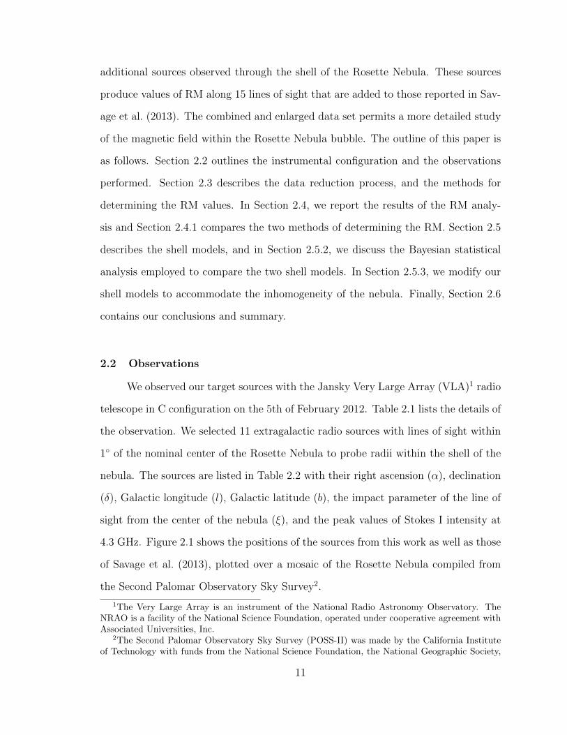
additional sources observed through the shell of the Rosette Nebula. These sources

produce values of RM along 15 lines of sight that are added to those reported in Sav-

age et al. (2013). The combined and enlarged data set permits a more detailed study

of the magnetic field within the Rosette Nebula bubble. The outline of this paper is

as follows. Section 2.2 outlines the instrumental configuration and the observations

performed. Section 2.3 describes the data reduction process, and the methods for

determining the RM values. In Section 2.4, we report the results of the RM analy-

sis and Section 2.4.1 compares the two methods of determining the RM. Section 2.5

describes the shell models, and in Section 2.5.2, we discuss the Bayesian statistical

analysis employed to compare the two shell models. In Section 2.5.3, we modify our

shell models to accommodate the inhomogeneity of the nebula. Finally, Section 2.6

contains our conclusions and summary.

2.2 Observations

We observed our target sources with the Jansky Very Large Array (VLA)1 radio

telescope in C configuration on the 5th of February 2012. Table 2.1 lists the details of

the observation. We selected 11 extragalactic radio sources with lines of sight within

1 of the nominal center of the Rosette Nebula to probe radii within the shell of the

nebula. The sources are listed in Table 2.2 with their right ascension (α), declination

(δ), Galactic longitude (l), Galactic latitude (b), the impact parameter of the line of

sight from the center of the nebula (ξ), and the peak values of Stokes I intensity at

4.3 GHz. Figure 2.1 shows the positions of the sources from this work as well as those

of Savage et al. (2013), plotted over a mosaic of the Rosette Nebula compiled from

the Second Palomar Observatory Sky Survey2.

1The Very Large Array is an instrument of the National Radio Astronomy Observatory. TheNRAO is a facility of the National Science Foundation, operated under cooperative agreement withAssociated Universities, Inc.

2The Second Palomar Observatory Sky Survey (POSS-II) was made by the California Instituteof Technology with funds from the National Science Foundation, the National Geographic Society,

11

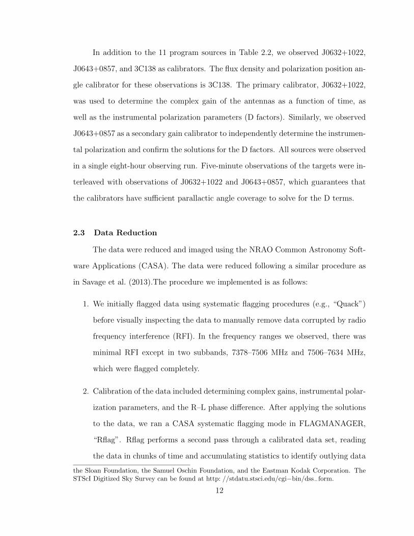
In addition to the 11 program sources in Table 2.2, we observed J0632+1022,

J0643+0857, and 3C138 as calibrators. The flux density and polarization position an-

gle calibrator for these observations is 3C138. The primary calibrator, J0632+1022,

was used to determine the complex gain of the antennas as a function of time, as

well as the instrumental polarization parameters (D factors). Similarly, we observed

J0643+0857 as a secondary gain calibrator to independently determine the instrumen-

tal polarization and confirm the solutions for the D factors. All sources were observed

in a single eight-hour observing run. Five-minute observations of the targets were in-

terleaved with observations of J0632+1022 and J0643+0857, which guarantees that

the calibrators have sufficient parallactic angle coverage to solve for the D terms.

2.3 Data Reduction

The data were reduced and imaged using the NRAO Common Astronomy Soft-

ware Applications (CASA). The data were reduced following a similar procedure as

in Savage et al. (2013).The procedure we implemented is as follows:

1. We initially flagged data using systematic flagging procedures (e.g., “Quack”)

before visually inspecting the data to manually remove data corrupted by radio

frequency interference (RFI). In the frequency ranges we observed, there was

minimal RFI except in two subbands, 7378–7506 MHz and 7506–7634 MHz,

which were flagged completely.

2. Calibration of the data included determining complex gains, instrumental polar-

ization parameters, and the R–L phase difference. After applying the solutions

to the data, we ran a CASA systematic flagging mode in FLAGMANAGER,

“Rflag”. Rflag performs a second pass through a calibrated data set, reading

the data in chunks of time and accumulating statistics to identify outlying data

the Sloan Foundation, the Samuel Oschin Foundation, and the Eastman Kodak Corporation. TheSTScI Digitized Sky Survey can be found at http: //stdatu.stsci.edu/cgi−bin/dss−form.

12

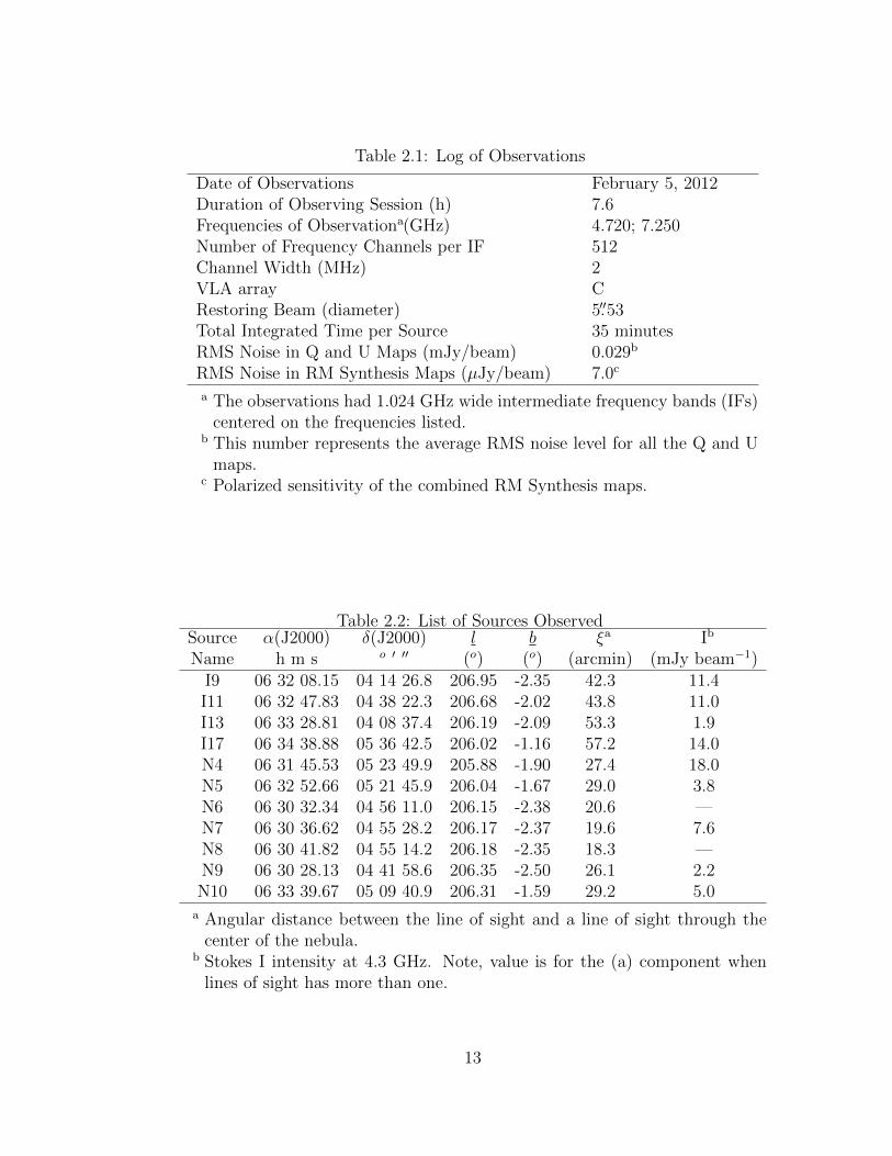
Table 2.1: Log of Observations

Date of Observations February 5, 2012Duration of Observing Session (h) 7.6Frequencies of Observationa(GHz) 4.720; 7.250Number of Frequency Channels per IF 512Channel Width (MHz) 2VLA array CRestoring Beam (diameter) 5.′′53Total Integrated Time per Source 35 minutesRMS Noise in Q and U Maps (mJy/beam) 0.029b

RMS Noise in RM Synthesis Maps (µJy/beam) 7.0c

a The observations had 1.024 GHz wide intermediate frequency bands (IFs)centered on the frequencies listed.

b This number represents the average RMS noise level for all the Q and Umaps.

c Polarized sensitivity of the combined RM Synthesis maps.

Table 2.2: List of Sources ObservedSource α(J2000) δ(J2000) l b ξa Ib

Name h m s o ′ ′′ (o) (o) (arcmin) (mJy beam−1)I9 06 32 08.15 04 14 26.8 206.95 -2.35 42.3 11.4I11 06 32 47.83 04 38 22.3 206.68 -2.02 43.8 11.0I13 06 33 28.81 04 08 37.4 206.19 -2.09 53.3 1.9I17 06 34 38.88 05 36 42.5 206.02 -1.16 57.2 14.0N4 06 31 45.53 05 23 49.9 205.88 -1.90 27.4 18.0N5 06 32 52.66 05 21 45.9 206.04 -1.67 29.0 3.8N6 06 30 32.34 04 56 11.0 206.15 -2.38 20.6 —N7 06 30 36.62 04 55 28.2 206.17 -2.37 19.6 7.6N8 06 30 41.82 04 55 14.2 206.18 -2.35 18.3 —N9 06 30 28.13 04 41 58.6 206.35 -2.50 26.1 2.2N10 06 33 39.67 05 09 40.9 206.31 -1.59 29.2 5.0

a Angular distance between the line of sight and a line of sight through thecenter of the nebula.

b Stokes I intensity at 4.3 GHz. Note, value is for the (a) component whenlines of sight has more than one.

13

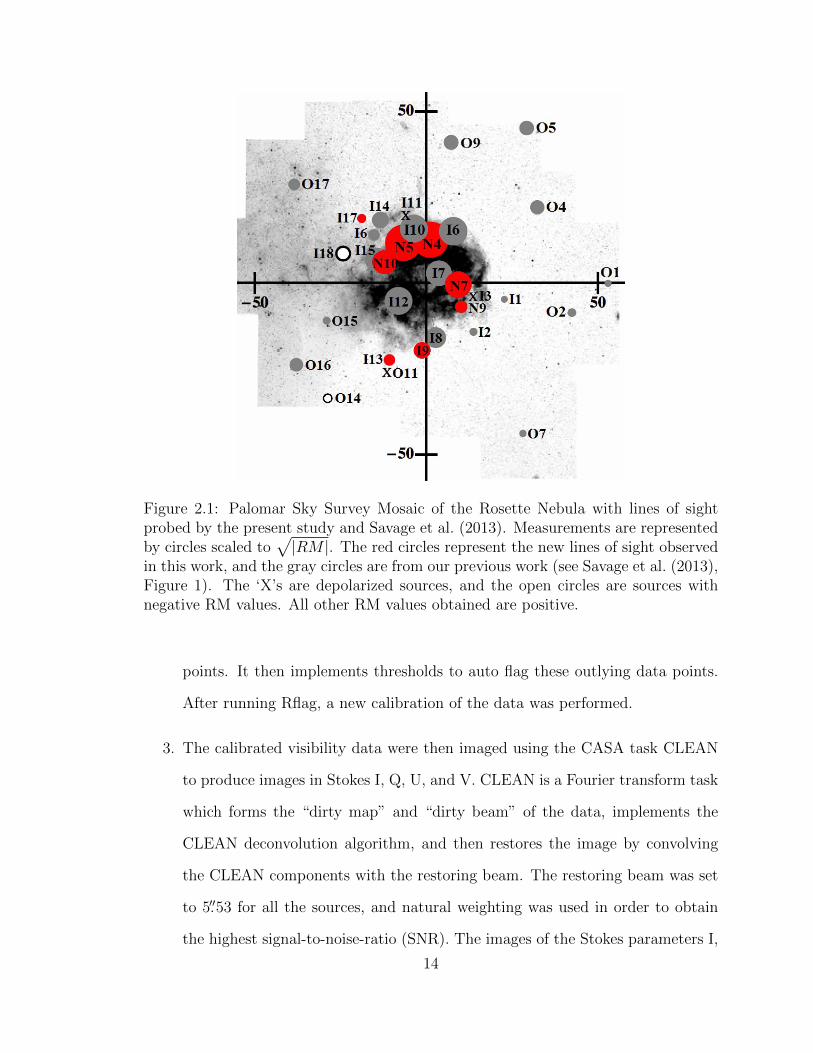
Figure 2.1: Palomar Sky Survey Mosaic of the Rosette Nebula with lines of sightprobed by the present study and Savage et al. (2013). Measurements are representedby circles scaled to

√|RM |. The red circles represent the new lines of sight observed

in this work, and the gray circles are from our previous work (see Savage et al. (2013),Figure 1). The ‘X’s are depolarized sources, and the open circles are sources withnegative RM values. All other RM values obtained are positive.

points. It then implements thresholds to auto flag these outlying data points.

After running Rflag, a new calibration of the data was performed.

3. The calibrated visibility data were then imaged using the CASA task CLEAN

to produce images in Stokes I, Q, U, and V. CLEAN is a Fourier transform task

which forms the “dirty map” and “dirty beam” of the data, implements the

CLEAN deconvolution algorithm, and then restores the image by convolving

the CLEAN components with the restoring beam. The restoring beam was set

to 5.′′53 for all the sources, and natural weighting was used in order to obtain

the highest signal-to-noise-ratio (SNR). The images of the Stokes parameters I,

14

Q, U, and V were made in two ways. These two sets of images were the input

data for the two methods of determining the RM, described further in Sections

2.3.1.1 and 2.3.1.2.

(a) In the first approach, a single image of each Stokes parameter was made

in 128 MHz-wide subbands within each 1.024 GHz intermediate frequency

band (IFs). The actual spectrum utilized was sightly less than 128 MHz

because of discarded edge channels as well as channels lost to RFI. Since the

bandwidth of 128 MHz is non-negligible compared to the center frequency,

particularly for the lower frequency subbands, we used the “mfs” (multi-

frequency synthesis) mode in the task CLEAN. This algorithm takes into

account the different (u, v) tracks corresponding to different frequencies.

The image resulting from mfs CLEAN corresponds to a frequency at the

center of the 128 MHz-wide subband. These images were the inputs to the

χ(λ2) analysis (Section 2.3.1.1).

(b) The second approach was to make I, Q, U, and V images for each 4 MHz-

wide piece of spectrum in our observations using the mode “channel” in

CASA, which averages two adjacent 2 MHz channels. The resulting set of

maps were used as input to the RM synthesis analysis (Section 2.3.1.2).

4. Finally, phase-only self-calibration was performed on all sources. For the sources

with sufficient SNR (i.e., SNR > 20 )3 , we performed two iterations of phase-

only self-calibration. The sources with SNR < 20 did not improve with phase-

only self-calibration.

3NRAO Data Reduction Workshop 2012

15

2.3.1 Determination of Rotation Measures Using Two Techniques

For all 11 sources, we employ two methods to determine the RM for each source

or source component. The first method (Section 2.3.1.1) was implemented in Savage

et al. (2013) and consists of a least-squares linear fit of χ(λ2). This is a technique

that has traditionally been used to measure Faraday rotation from radio astronomical

polarization measurements. The second method (Section 2.3.1.2) is Rotation Measure

Synthesis (RM Synthesis) (Brentjens & de Bruyn, 2005). RM Synthesis exploits the

large, multi-channel data sets generated by modern interferometers like the VLA and

avoids some of the shortcomings of the χ(λ2) fit. The following sections detail the

imaging process for the two methods.

2.3.1.1 Rotation Measures from Least-Squares Fit of χ(λ2)

The output of the CASA task CLEAN is a set of images in Stokes I, Q, U, and

V. With these images, we use the CASA task IMMATH to generate maps of linear

polarized intensity P,

P =√Q2 + U2,

and the polarization position angle, χ,

χ =1

2tan−1

(U

Q

).

Figures 2.2a and 2.2b are examples of maps for two sources, where the vectors are

χ, the gray scale is P, and the contours are the Stokes I intensity. Though some of

the sources observed in this project are point sources to the VLA in C array, other

sources like N10 (Figure 2.2b) have resolvable structure. For each source, we produce

maps in each of the fourteen, 128 MHz-wide subbands. To obtain measurements of

16

χ, we select the pixel of the highest value of P of the source in the 4338 MHz map

and measure χ at that location in each 128 MHz-wide subband.

(a) (b)

Figure 2.2: Map of (a) N4 and (b) N10 at 4.85 GHz. The gray scale is the linearpolarized intensity, P, the vectors show the polarization position angle, χ, and thecontours are the Stokes I intensity with levels of -2, -1 , 2, 10, 20, 40, 60, and 80% of thepeak intensity, 24.5 mJy beam−1 and 4.87 mJy beam−1 for N4 and N10, respectively.The circle in the lower left is the restoring beam. In image (b), there are four resolvedcomponents of N10, and we call the northern component “a” in Table 2.3 and thefollowing three components are marked “b”–“d” in a clockwise direction from “a”.

0.002 0.0035 0.005

-2

1

-1

0

2

Λ2 Im2M

ΧHra

dL

Figure 2.3: Plot of the polarization position angle as a function of the square of thewavelength, χ(λ2), for the source N4, RM= +1383 ± 18 rad m−2. The reduced χ2

is 1.5. Each plotted point results from a measurement in a single 128 MHz-widesubband.

17

0.001 0.002 0.003 0.004 0.0050.51.01.52.02.53.03.5

Λ2 Im2M

mH%

L

(a)

0.001 0.002 0.003 0.004 0.0058

9

10

11

12

Λ2 Im2M

mH%

L

(b)

Figure 2.4: Graph of the percent polarization, m, as a function of λ2 for sources(a) I9 and (b) I17. These sources show a decrease in m with increasing λ2, whichis characteristic of depolarization. The dashed line shows the median value of thepercent polarization.

We obtain RM measurements by carrying out a least-squares linear fit of χ(λ2),

where RM is the slope of the line. Figure 2.3 shows an example of the least-squares fit

for the source N4. The errors in χ are σχ =σQ2P

(Everett & Weisberg 2001, Equation

(12)), where σQ = σU is the rms noise in the Q map. This method assumes that

there is only one source along the line of sight, unaffected by beam depolarization

and without internal Faraday rotation. Depolarization manifests itself as a change in

m=P/I with frequency. Depolarization may occur for a number of reasons, such as

external Faraday dispersion, multiple interfering RM components, differential Faraday

rotation, or internal Faraday rotation (Burn, 1966; Sokoloff et al., 1998; O’Sullivan

et al., 2012).

For all sources, we inspected plots of m(λ2) to determine if there were depolar-

ization effects. Figures 2.4a and 2.4b show the graphs for the two sources, I9 and I17,

respectively, which show depolarization. Despite the detection of depolarization for

these two sources, we do not believe our resultant RM values to be biased or in error.

The reduced χ2 of the fit of χ(λ2) is satisfactory and suggests no departure from the

χ vs λ2 dependence (Table 2.3).

18

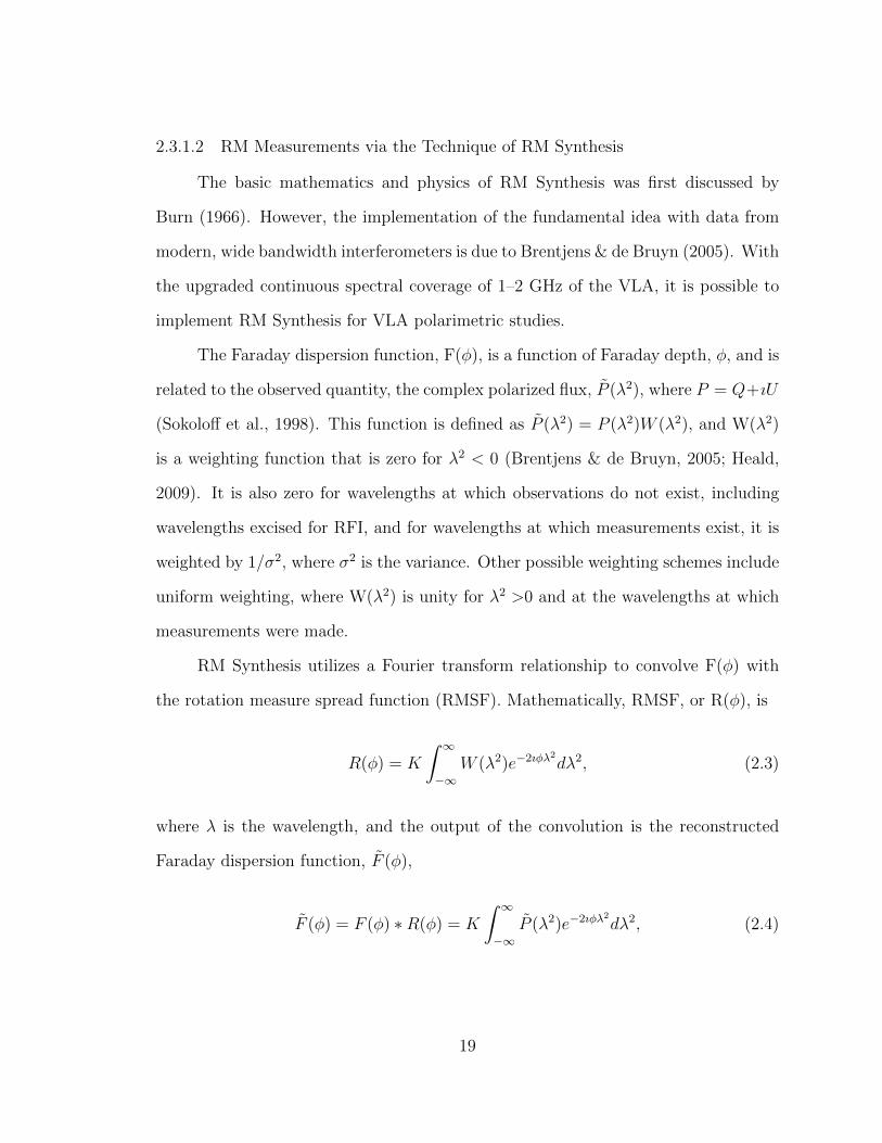
2.3.1.2 RM Measurements via the Technique of RM Synthesis

The basic mathematics and physics of RM Synthesis was first discussed by

Burn (1966). However, the implementation of the fundamental idea with data from

modern, wide bandwidth interferometers is due to Brentjens & de Bruyn (2005). With

the upgraded continuous spectral coverage of 1–2 GHz of the VLA, it is possible to

implement RM Synthesis for VLA polarimetric studies.

The Faraday dispersion function, F(φ), is a function of Faraday depth, φ, and is

related to the observed quantity, the complex polarized flux, P (λ2), where P = Q+ıU

(Sokoloff et al., 1998). This function is defined as P (λ2) = P (λ2)W (λ2), and W(λ2)

is a weighting function that is zero for λ2 < 0 (Brentjens & de Bruyn, 2005; Heald,

2009). It is also zero for wavelengths at which observations do not exist, including

wavelengths excised for RFI, and for wavelengths at which measurements exist, it is

weighted by 1/σ2, where σ2 is the variance. Other possible weighting schemes include

uniform weighting, where W(λ2) is unity for λ2 >0 and at the wavelengths at which

measurements were made.

RM Synthesis utilizes a Fourier transform relationship to convolve F(φ) with

the rotation measure spread function (RMSF). Mathematically, RMSF, or R(φ), is

R(φ) = K

∫ ∞−∞

W (λ2)e−2ıφλ2dλ2, (2.3)

where λ is the wavelength, and the output of the convolution is the reconstructed

Faraday dispersion function, F (φ),

F (φ) = F (φ) ∗R(φ) = K

∫ ∞−∞

P (λ2)e−2ıφλ2dλ2, (2.4)

19

where K is a normalization function given by

K =

(∫ ∞−∞

W (λ2)dλ2

)−1

,

(see Brentjens & de Bruyn (2005) for the full derivation). To recover F(φ), F (φ)

is deconvolved via a CLEAN algorithm such as the ones discussed in Heald (2009)

and Bell & Enßlin (2012). In the case of a single point source behind a Faraday

screen, F(φ) is a delta function at a Faraday depth equal to the RM through the

screen. “Faraday Complexity” (Anderson et al., 2015) will lead to a broadening of

the Faraday dispersion function, F(φ), and Q and U will have non-sinusoidal behavior.

This broadening can also occur in the case of depolarization of a single component.

Figure 2.5: KVIS output map from the RM Synthesis analysis where the gray scaleis the polarized intensity for the source N4 at φ=+1408 rad m−2.

In practice, we utilize an IDL implementation of an RM Synthesis and CLEAN

code. The inputs to the IDL code are FITS files of the CLEANed images of Stokes

Q and U exported from CASA. The Q and U images are a function of frequency,

Q(ν) and U(ν), and are composed of fourteen subbands containing twenty-four 4

MHz-wide channels. Ideally, an RFI free data set would permit the use of all sixteen

20

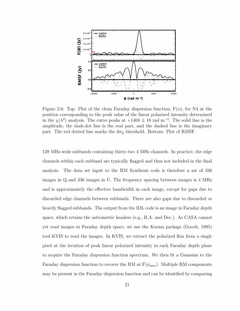
Figure 2.6: Top: Plot of the clean Faraday dispersion function, F(φ), for N4 at theposition corresponding to the peak value of the linear polarized intensity determinedin the χ(λ2) analysis. The curve peaks at +1408 ± 16 rad m−2. The solid line is theamplitude, the dash-dot line is the real part, and the dashed line is the imaginarypart. The red dotted line marks the 3σQ threshold. Bottom: Plot of RMSF.

128 MHz-wide subbands containing thirty-two 4 MHz channels. In practice, the edge

channels within each subband are typically flagged and thus not included in the final

analysis. The data set input to the RM Synthesis code is therefore a set of 336

images in Q and 336 images in U. The frequency spacing between images is 4 MHz

and is approximately the effective bandwidth in each image, except for gaps due to

discarded edge channels between subbands. There are also gaps due to discarded or

heavily flagged subbands. The output from the IDL code is an image in Faraday depth

space, which retains the astrometric headers (e.g., R.A. and Dec.). As CASA cannot

yet read images in Faraday depth space, we use the Karma package (Gooch, 1995)

tool KVIS to read the images. In KVIS, we extract the polarized flux from a single

pixel at the location of peak linear polarized intensity in each Faraday depth plane

to acquire the Faraday dispersion function spectrum. We then fit a Gaussian to the

Faraday dispersion function to recover the RM at F(φmax). Multiple RM components

may be present in the Faraday dispersion function and can be identified by comparing

21

the data to the RMSF. The Faraday dispersion function was measured at the same

spatial location as used for the χ(λ2) analysis, for each source or source component.

This was done so that we can compare the two measurements.

For each source, we implemented a search range of φ = ± 10000 rad m−2 to

identify possible peaks at large values of φ. We are sensitive up to φmax ∼ 3.0×105 rad

m−2, the full width at half-maximum (FWHM) of the RMSF is φFWHM = 1067 rad

m−2, and the largest detectable scale in Faraday depth space (max-scale) is 2085 rad

m−2(see Equations (61)–(63) in Brentjens & de Bruyn 2005). In Table 2.3, column 5

lists the effective RM values derived from the peak of the Faraday dispersion function

from the RM Synthesis analysis.

Figure 2.5 shows an example of a KVIS map for source N4 at φ = 1408 rad

m−2. The top panel of Figure 2.6 is the Faraday dispersion function corresponding to

one pixel from Figure 2.5, and the bottom panel plots the RMSF. Using the spatial

location of the peak linear polarized intensity from the χ(λ2) analysis, we select the

same spatial location on the RM Synthesis map so that we may compare the two

measurements. In general, this method samples the Faraday dispersion function at

F(φpeak) and at Pmax in the RM Synthesis data. The exception to this is N9(b).

The spatial location of F(φmax) in the RM Synthesis map does not coincide with the

location in the χ(λ2) maps, which is most likely due to the values of P not exceeding

the 5σQ threshold that is implemented in the imaging process in CASA (see Section

2.4.1) in the χ(λ2) analysis. The reported RM value derived from the RM Synthesis

analysis is spatially coincident with the χ(λ2) value to maintain consistency.

2.4 Observational Results

For the 11 sources observed through the shell of the Rosette Nebula, we mea-

sured RM values for fifteen lines of sight, including secondary components. Table

2.3 lists the RM values and associated errors for the least-squares method and from

22

the RM Synthesis analysis. We have three lines of sight that do not pass through

the shell of the nebula, I9, I13, and I17. Including the secondary components, we

measure an average background RM due to the general ISM of +146 ± 37 rad m−2.

The background RM is in perfect agreement with the value from Savage et al. (2013).

We see no evidence for a gradient in the measured background RM values over the

4 diameter region centered on the nebula. We measure an excess RM ranging from

+40 to +1200 rad m−2 due to the shell of the nebula. Figure 2.1 shows the new

sources in red in combination with the results from Savage et al. (2013), where the

symbols are scaled to√|RM |. Figure 2.7 plots the observed RM measurements as

a function of distance from in the center of the Rosette Nebula in parsecs, using a

distance of 1600 pc to the nebula (Roman-Zuniga & Lada, 2008).

Double or multiple sources with large changes in RM values can probe small

scale structure in the Rosette Nebula. We use the variable ∆RM to indicate differ-

ences in the RM between components or parts of a source with angular separations

larger than the restoring beam of 5.′′5. Of the 8 sources with RMs, 5 sources have

more than one component that yield RM values. N10 has a maximum angular sep-

aration of 53′′ between the northern and the southern component and 13′′ between

the eastern and western components. For I13 and I17, the angular separations are

30′′ and 10′′, respectively. In these cases, the ∆RM values are relatively small, nearly

within the errors in the case of I17. The ∆RM values for N5 and N9, however, appear

to be significant, with ∆RM ∼ 350 and 260 rad m−2 for N5 and N9, respectively. The

angular separation between the components for N5 is 18′′, and N9 has a separation

of 50′′. The linear separations between the components for these sources are 0.14 and

0.39 pc, respectively. Our measurements of ∆ RM may indicate small scale gradients

in the electron density or line-of-sight component of the magnetic field in the Rosette

Nebula. These variations could be due to inhomogeneities in the shell, or turbulent

fluctuations in ne and B‖ on spatial scales of 0.1 to 1 parsec.

23

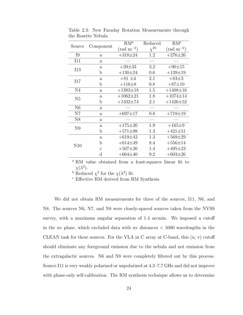
Table 2.3: New Faraday Rotation Measurements throughthe Rosette Nebula

Source ComponentRMa Reduced RMc

(rad m−2) χ2b (rad m−2)I9 a +318±24 1.2 +276±26I11 a — — —

I13a +39±33 3.2 +90±15b +130±24 0.6 +139±19

I17a +81 ±4 2.1 +83±3b +116±8 0.8 +87±10

N4 a +1383±18 1.5 +1408±16

N5a +1062±21 1.8 +1074±14b +1332±74 2.1 +1426±52

N6 a — — —N7 a +697±17 0.8 +719±19N8 a — — —

N9a +175±20 1.9 +165±9b +571±98 1.3 +421±51

N10

a +619±42 1.3 +569±29b +614±49 8.4 +556±14c +507±20 1.4 +495±23d +664±40 9.2 +603±26

a RM value obtained from a least-squares linear fit toχ(λ2).

b Reduced χ2 for the χ(λ2) fit.c Effective RM derived from RM Synthesis

We did not obtain RM measurements for three of the sources, I11, N6, and

N8. The sources N6, N7, and N8 were closely-spaced sources taken from the NVSS

survey, with a maximum angular separation of 1.4 arcmin. We imposed a cutoff

in the uv plane, which excluded data with uv distances < 5000 wavelengths in the

CLEAN task for these sources. For the VLA in C array at C-band, this (u, v) cutoff

should eliminate any foreground emission due to the nebula and not emission from

the extragalactic sources. N6 and N8 were completely filtered out by this process.

Source I11 is very weakly polarized or unpolarized at 4.3–7.7 GHz and did not improve

with phase-only self-calibration. The RM synthesis technique allows us to determine

24

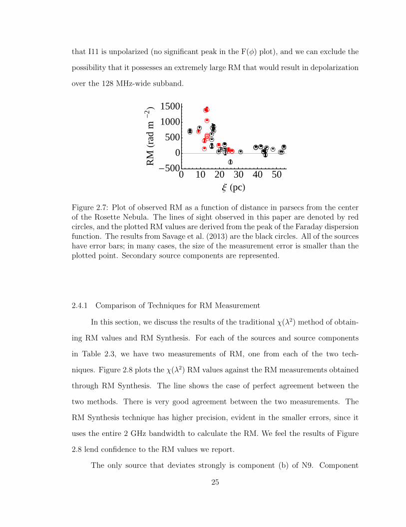
that I11 is unpolarized (no significant peak in the F(φ) plot), and we can exclude the

possibility that it possesses an extremely large RM that would result in depolarization

over the 128 MHz-wide subband.

0 10 20 30 40 50-500

0

500

1000

1500

Ξ HpcL

RM

Hrad

m-

2L

Figure 2.7: Plot of observed RM as a function of distance in parsecs from the centerof the Rosette Nebula. The lines of sight observed in this paper are denoted by redcircles, and the plotted RM values are derived from the peak of the Faraday dispersionfunction. The results from Savage et al. (2013) are the black circles. All of the sourceshave error bars; in many cases, the size of the measurement error is smaller than theplotted point. Secondary source components are represented.

2.4.1 Comparison of Techniques for RM Measurement

In this section, we discuss the results of the traditional χ(λ2) method of obtain-

ing RM values and RM Synthesis. For each of the sources and source components

in Table 2.3, we have two measurements of RM, one from each of the two tech-

niques. Figure 2.8 plots the χ(λ2) RM values against the RM measurements obtained

through RM Synthesis. The line shows the case of perfect agreement between the

two methods. There is very good agreement between the two measurements. The

RM Synthesis technique has higher precision, evident in the smaller errors, since it

uses the entire 2 GHz bandwidth to calculate the RM. We feel the results of Figure

2.8 lend confidence to the RM values we report.

The only source that deviates strongly is component (b) of N9. Component

25

0 500 1000 15000

500

1000

1500

Least Squares RM

RM

Synth

esis

Figure 2.8: Plot comparing the RM measurements (rad m−2) obtained from RM Syn-thesis and the traditional least-squares fitting method of χ(λ2). The line representsperfect agreement between the two measurements, and errors for both methods arerepresented.

(b) of N9 is a weak source. The Stokes I intensity at 4.3GHz ∼1.2 mJy beam−1.

N9(b) did not improve with phase-only self-calibration, and the linear polarized in-

tensity only exceeds the 5σQ threshold in one subband in the χ(λ2) analysis. N9(b)

is present, however, in the RM Synthesis analysis. RM Synthesis has the advantage

over the χ(λ2) method of being less sensitive to low SNR levels than the traditional

χ(λ2) method. In spite of the large errors associated with the components of N9, the

difference in ∆RM is large enough to be significant. In our analysis in the following

sections, we use the RM values derived from the RM Synthesis technique for all of

the sources.

2.5 Diagnostics of Magnetic Fields in H ii Regions Utilizing Plasma Shell

Models

2.5.1 Empirical Models for Stellar Bubbles

Savage et al. (2013) employed a physically motivated shell model to represent

26

the magnitude and spatial distribution of the observed RM in the shell of the Rosette

Nebula. The equation describing this shell model is

RM(ξ) =CneL(ξ)

2[BzI +BzE], (2.5)

where BzI and BzE are the line of sight components of the magnetic field in the shell

at ingress and egress, respectively, and C is a set of constants equal to 0.81 defined

by Equation (2.2) when L(ξ), B, and ne are measured in parsecs, µGauss, and cm−3,

respectively (see Equation (10) in Whiting et al. 2009). BzI and BzE are defined to be

in the shell, and downstream from the hypothesized outer shock that defines the outer

limit of the bubble. Relations between BzI and BzE and the upstream, undisturbed

ISM magnetic field are given in Equations (6)–(9) of Whiting et al. (2009). L(ξ) is

the chord length through the shell, and it has two domains given by

L(ξ) = 2R0

√√√√(1−(ξ

R0

)2)

, if ξ ≥ R1 , and (2.6)

L(ξ) = 2R0

√√√√(1−

(ξ

R0

)2)−(R1

R0

)√√√√(1−(ξ

R1

)2) , if ξ ≤ R1,

where R0 and R1 are the outer and inner radii of the shell, respectively, and ξ is the

distance between the line of sight and the center of the shell (see Figure 6 of Whiting

et al. 2009). Outside the outer radius of the H ii region (R0 < ξ), the model predicts

RM=0, so the background RM due to the Galactic plane in this region is determined

empirically through observations in the vicinity of, but outside the Rosette Nebula.

The external general interstellar magnetic field, B0, can be treated as a constant,

meaning we assume B0 does not vary significantly over the extent of the Rosette

Nebula, i.e., outside the nebula, B0 is constant in magnitude and direction. At the

27

shock front located at R0, B0 can be decomposed into components perpendicular (B⊥)

and parallel (B‖) to the shock normal. The perpendicular component is amplified by

the density compression ratio (X) in the shell. Use of all these considerations then

gives (Savage et al. 2013, Equation (8))

RM = CneL(ξ)B0z

(1 + (X − 1)

(ξ

R0

)2). (2.7)

B0z is the z-component of B0, such that

B0z = B0 cos θ, (2.8)

where B0 is the magnitude of the ISM magnetic field and θ, the angle between the

direction to Earth and B0, becomes the only free parameter in the model. We assume

B0 to be a constant and known. K. Ferriere (private communication) has pointed out

that in reality, there will be fluctuations in |B0| as well as θ in the interstellar medium.

As a result, it can be argued that B0z should be considered the true independent

parameter in Equation (2.7). In the limit of a purely adiabatic strong shock, i.e.,

X=4, Equation (2.7) predicts that the maximum value of the RM occurs near the

outer radius of the shell for ξ < R0. As discussed in Section 2.1.1, Harvey-Smith

et al. (2011) consider a case in which the increase in RM is due solely to an increase

in density and not the magnetic field. In this limit where X=1, Equation (2.7) models

the expected RM in the shell without an enhancement in the magnetic field,

RM(ξ) = CneL(ξ)B0z (2.9)

and it predicts the maximum value of the RM is at the contact discontinuity, R1.

Equations (2.7) and (2.9) represent two different models for the structure of the

bubble, albeit highly simplified and approximate. The model described by Equation

28

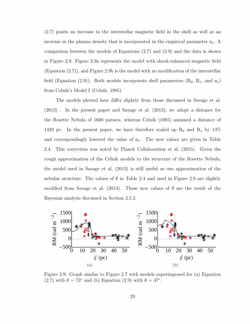
(2.7) posits an increase in the interstellar magnetic field in the shell as well as an

increase in the plasma density that is incorporated in the empirical parameter ne. A

comparison between the models of Equations (2.7) and (2.9) and the data is shown

in Figure 2.9. Figure 2.9a represents the model with shock-enhanced magnetic field

(Equation (2.7)), and Figure 2.9b is the model with no modification of the interstellar

field (Equation (2.9)). Both models incorporate shell parameters (R0, R1, and ne)

from Celnik’s Model I (Celnik, 1985).

The models plotted here differ slightly from those discussed in Savage et al.

(2013) . In the present paper and Savage et al. (2013), we adopt a distance for

the Rosette Nebula of 1600 parsecs, whereas Celnik (1985) assumed a distance of

1420 pc. In the present paper, we have therefore scaled up R0 and R1 by 13%

and correspondingly lowered the value of ne. The new values are given in Table

2.4. This correction was noted by Planck Collaboration et al. (2015). Given the

rough approximation of the Celnik models to the structure of the Rosette Nebula,

the model used in Savage et al. (2013) is still useful as one approximation of the

nebular structure. The values of θ in Table 2.4 and used in Figure 2.9 are slightly

modified from Savage et al. (2013). These new values of θ are the result of the

Bayesian analysis discussed in Section 2.5.2.

0 10 20 30 40 50-500

0

500

1000

1500

Ξ HpcL

RM

Hrad

m-

2L

(a)

0 10 20 30 40 50-500

0

500

1000

1500

Ξ HpcL

RM

Hrad

m-

2L

(b)

Figure 2.9: Graph similar to Figure 2.7 with models superimposed for (a) Equation(2.7) with θ = 73 and (b) Equation (2.9) with θ = 47.

29

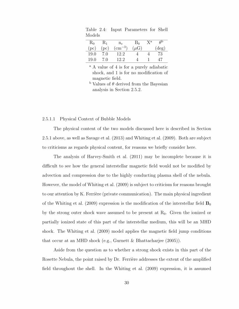
Table 2.4: Input Parameters for ShellModels

R0 R1 ne B0 Xa θb

(pc) (pc) (cm−3) (µG) (deg)19.0 7.0 12.2 4 4 7319.0 7.0 12.2 4 1 47a A value of 4 is for a purely adiabatic

shock, and 1 is for no modification ofmagnetic field.

b Values of θ derived from the Bayesiananalysis in Section 2.5.2.

2.5.1.1 Physical Context of Bubble Models

The physical content of the two models discussed here is described in Section

2.5.1 above, as well as Savage et al. (2013) and Whiting et al. (2009). Both are subject

to criticisms as regards physical content, for reasons we briefly consider here.

The analysis of Harvey-Smith et al. (2011) may be incomplete because it is

difficult to see how the general interstellar magnetic field would not be modified by

advection and compression due to the highly conducting plasma shell of the nebula.

However, the model of Whiting et al. (2009) is subject to criticism for reasons brought

to our attention by K. Ferriere (private communication). The main physical ingredient

of the Whiting et al. (2009) expression is the modification of the interstellar field B0

by the strong outer shock wave assumed to be present at R0. Given the ionized or

partially ionized state of this part of the interstellar medium, this will be an MHD

shock. The Whiting et al. (2009) model applies the magnetic field jump conditions

that occur at an MHD shock (e.g., Gurnett & Bhattacharjee (2005)).

Aside from the question as to whether a strong shock exists in this part of the

Rosette Nebula, the point raised by Dr. Ferriere addresses the extent of the amplified

field throughout the shell. In the Whiting et al. (2009) expression, it is assumed

30

that the amplified field applies to a large portion of the shell (see fuller discussion

in Whiting et al. 2009). Dr. Ferriere’s point is that while this simplification might

be valid in the case of a thin shell, it becomes questionable in the case of an object

like the Rosette Nebula, in which the shell between R1 and R0 occupies most of the

volume of the nebula.

The points raised by Dr. Ferriere are included in Planck Collaboration et al.

(2015) (Section 5 and Appendix A). That paper also includes a model of the nebular

field based on the assumption of conservation of magnetic flux. While recognizing the

points raised above, we will continue to use the expressions contained in Equations

(2.7) and (2.9) as part of the discussion in the present paper. These expressions

represent limiting behavior of the magnetic field within a bubble shell. For example,

Equation (2.7) may be considered a proxy for any mechanism that would enhance the

interstellar field within the nebular bubble, and rotate it into a plane perpendicular

to the radial direction. It is perhaps worth pointing out that the RM(ξ) curves

presented by Planck Collaboration et al. (2015) in their Figure 5 also show “rotation

measure limb brightening” that is characteristic of the Whiting model. In Figure 5(a)

of Planck Collaboration et al. (2015), the peak of the curve is located at ξ ∼12 – 13

pc for the blue and red curves, respectively. This peak is only slightly interior to

where the peak of Equation (2.7) is located at ξ ∼ 14.2 pc. In both Equations (2.7)

and (2.9), the discontinuity in the derivative of RM at R1 results from the assumption

that a contact discontinuity occurs here. Furthermore, both models assume the region

interior to R1 is a vacuum. In any case, the comparison of measurements to a set

of simplified descriptions of magnetic field behavior should further the goal of these

investigations, which is to better specify the magnetic field within these shells, and

how they are related to the general interstellar magnetic field.

31

2.5.2 A Bayesian Statistical Approach to Compare Shell Models and Determine the

Orientation of the Interstellar Magnetic Field

In this section, we carry out a Bayesian statistical analysis to determine which of

the models described in Section 5.1 better reproduces the observed RM measurements,

and therefore offers a better representation of the magnetic field in the Rosette Nebula.

The Bayesian analysis is suitable for our purposes because the two models may be

considered “hypotheses” that are being tested (Gregory, 2005). Our approach and

terminology follows that presented in Gregory (2005). We adopt from Celnik (1985)

the parameters for the shell such as the inner and outer radius, R1 and R0, and the

electron density, ne. These parameters have been scaled to the distance to the Rosette

Nebula of 1600 pc. As in Planck Collaboration et al. (2015), we adopt R1 = 7.0 pc,

R0 = 19.0 pc, and ne = 12.2 cm−3. We retain the value of 4 µG for the magnitude

of the external magnetic field, B0 (Ferriere, 2011). Given the measured and adopted

values of the parameters, the RM through the bubble is determined by the angle θ.

In Savage et al. (2013), a value of θ = 72 for a shell with an amplified magnetic

field was obtained by visually inspecting the fit of the model to the data. For the

model without the amplification of the magnetic field (Equation (2.9)), θ = 54. The

Bayesian analysis to be presented below automatically yields the optimum value of θ

for each model. Although the primary reason for carrying out the Bayesian analysis

is to determine which model better represents the observations, irrespective of the

value of θ, this quantity is nonetheless of astronomical interest.

Bayes’ Theorem states that the probability of a hypothesis being true given

some statement of prior information, is

p(Mi|D, I) =p(Mi|I)p(D|Mi, I)

p(D|I),

32

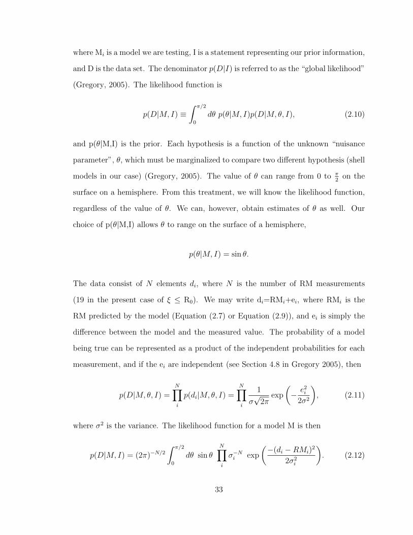
where Mi is a model we are testing, I is a statement representing our prior information,

and D is the data set. The denominator p(D|I) is referred to as the “global likelihood”

(Gregory, 2005). The likelihood function is

p(D|M, I) ≡∫ π/2

0

dθ p(θ|M, I)p(D|M, θ, I), (2.10)

and p(θ|M,I) is the prior. Each hypothesis is a function of the unknown “nuisance

parameter”, θ, which must be marginalized to compare two different hypothesis (shell

models in our case) (Gregory, 2005). The value of θ can range from 0 to π2

on the

surface on a hemisphere. From this treatment, we will know the likelihood function,

regardless of the value of θ. We can, however, obtain estimates of θ as well. Our

choice of p(θ|M,I) allows θ to range on the surface of a hemisphere,

p(θ|M, I) = sin θ.

The data consist of N elements di, where N is the number of RM measurements

(19 in the present case of ξ ≤ R0). We may write di=RMi+ei, where RMi is the

RM predicted by the model (Equation (2.7) or Equation (2.9)), and ei is simply the

difference between the model and the measured value. The probability of a model

being true can be represented as a product of the independent probabilities for each

measurement, and if the ei are independent (see Section 4.8 in Gregory 2005), then

p(D|M, θ, I) =N∏i

p(di|M, θ, I) =N∏i

1

σ√

2πexp

(− e2

i

2σ2

), (2.11)

where σ2 is the variance. The likelihood function for a model M is then

p(D|M, I) = (2π)−N/2∫ π/2

0

dθ sin θN∏i

σ−Ni exp

(−(di −RMi)

2

2σ2i

). (2.12)

33

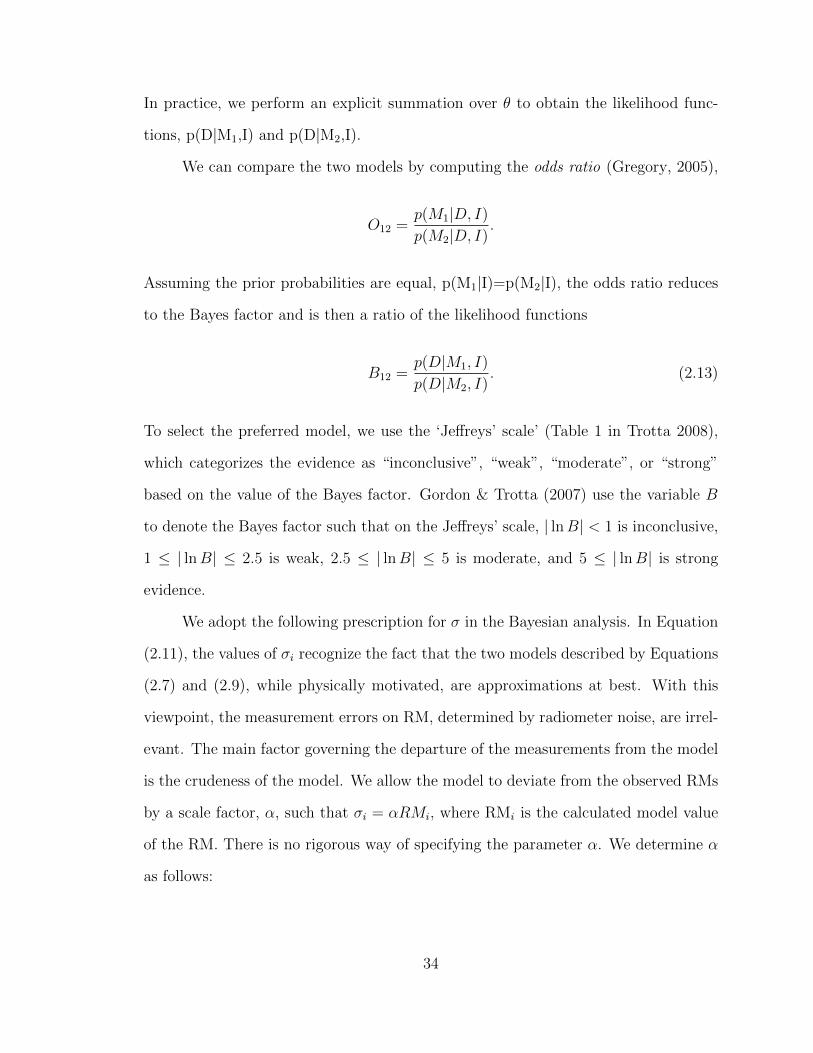
In practice, we perform an explicit summation over θ to obtain the likelihood func-

tions, p(D|M1,I) and p(D|M2,I).

We can compare the two models by computing the odds ratio (Gregory, 2005),

O12 =p(M1|D, I)

p(M2|D, I).

Assuming the prior probabilities are equal, p(M1|I)=p(M2|I), the odds ratio reduces

to the Bayes factor and is then a ratio of the likelihood functions

B12 =p(D|M1, I)

p(D|M2, I). (2.13)

To select the preferred model, we use the ‘Jeffreys’ scale’ (Table 1 in Trotta 2008),

which categorizes the evidence as “inconclusive”, “weak”, “moderate”, or “strong”

based on the value of the Bayes factor. Gordon & Trotta (2007) use the variable B

to denote the Bayes factor such that on the Jeffreys’ scale, | lnB| < 1 is inconclusive,

1 ≤ | lnB| ≤ 2.5 is weak, 2.5 ≤ | lnB| ≤ 5 is moderate, and 5 ≤ | lnB| is strong

evidence.

We adopt the following prescription for σ in the Bayesian analysis. In Equation

(2.11), the values of σi recognize the fact that the two models described by Equations

(2.7) and (2.9), while physically motivated, are approximations at best. With this

viewpoint, the measurement errors on RM, determined by radiometer noise, are irrel-

evant. The main factor governing the departure of the measurements from the model

is the crudeness of the model. We allow the model to deviate from the observed RMs

by a scale factor, α, such that σi = αRMi, where RMi is the calculated model value

of the RM. There is no rigorous way of specifying the parameter α. We determine α

as follows:

34

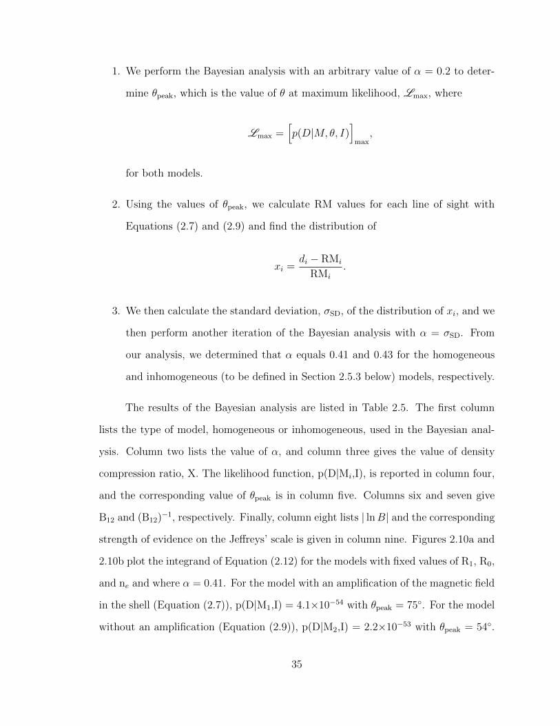
1. We perform the Bayesian analysis with an arbitrary value of α = 0.2 to deter-

mine θpeak, which is the value of θ at maximum likelihood, Lmax, where

Lmax =[p(D|M, θ, I)

]max

,

for both models.

2. Using the values of θpeak, we calculate RM values for each line of sight with

Equations (2.7) and (2.9) and find the distribution of

xi =di − RMi

RMi

.

3. We then calculate the standard deviation, σSD, of the distribution of xi, and we

then perform another iteration of the Bayesian analysis with α = σSD. From

our analysis, we determined that α equals 0.41 and 0.43 for the homogeneous

and inhomogeneous (to be defined in Section 2.5.3 below) models, respectively.

The results of the Bayesian analysis are listed in Table 2.5. The first column

lists the type of model, homogeneous or inhomogeneous, used in the Bayesian anal-

ysis. Column two lists the value of α, and column three gives the value of density

compression ratio, X. The likelihood function, p(D|Mi,I), is reported in column four,

and the corresponding value of θpeak is in column five. Columns six and seven give

B12 and (B12)−1, respectively. Finally, column eight lists | lnB| and the corresponding

strength of evidence on the Jeffreys’ scale is given in column nine. Figures 2.10a and

2.10b plot the integrand of Equation (2.12) for the models with fixed values of R1, R0,

and ne and where α = 0.41. For the model with an amplification of the magnetic field

in the shell (Equation (2.7)), p(D|M1,I) = 4.1×10−54 with θpeak = 75. For the model

without an amplification (Equation (2.9)), p(D|M2,I) = 2.2×10−53 with θpeak = 54.

35

The Bayes factor is B12 = 0.19 or B−112 = 5.4. Thus, | lnB| = 1.7, and this is consid-

ered “weak” evidence in favor of the model without an amplification of the magnetic

field in the shell, i.e., that considered by Harvey-Smith et al. (2011), on the Jeffreys’

scale. In this analysis, we have restricted the shell radii and the electron density to

be global parameters for the shell. The Bayesian analysis does not conclusively favor

either model. There is a weak tendency to favor the model without modification of

the general interstellar field.

36

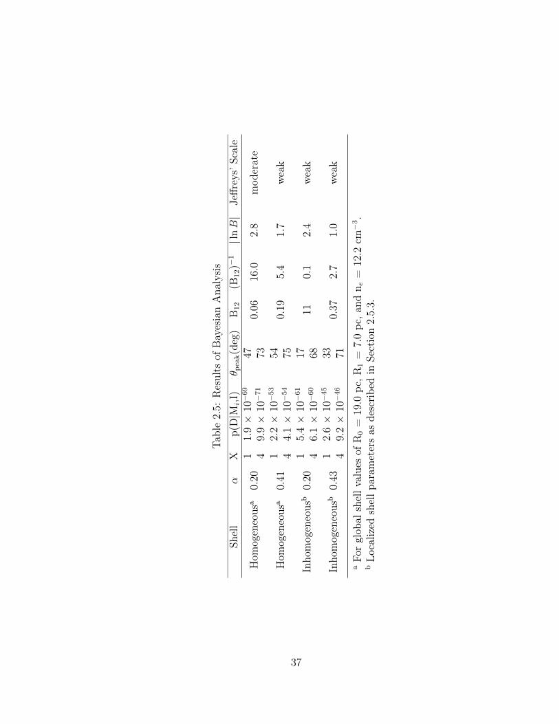
Tab

le2.

5:R

esult

sof

Bay

esia

nA

nal

ysi

s

Shel

lα

Xp(D|M

i,I)

θ pea

k(d

eg)

B12

(B12)−

1|l

nB|

Jeff

reys’

Sca

le

Hom

ogen

eousa

0.20

11.

9×

10−

69

470.

0616

.02.

8m

oder

ate

49.

9×

10−

71

73

Hom

ogen

eousa

0.41

12.

2×

10−

53

540.

195.

41.

7w

eak

44.

1×

10−

54

75

Inhom

ogen

eousb

0.20

15.

4×

10−

61

1711

0.1

2.4

wea

k4

6.1×

10−

60

68

Inhom

ogen

eousb

0.43

12.

6×

10−

45

330.

372.

71.

0w

eak

49.

2×

10−

46

71a

For

glob

alsh

ell

valu

esof

R0

=19

.0p

c,R

1=

7.0

pc,

and

ne

=12

.2cm−

3.

bL

oca

lize

dsh

ell

par

amet

ers

asdes

crib

edin

Sec

tion

2.5.

3.

37

0 20 40 60 80

5. ´ 10-61

1. ´ 10-60

1.5 ´ 10-60

1. ´ 10-61

Θ HdegLp

HΘÈM

,ILp

HDÈM

,Θ,I

L

(a)

0 20 40 60 80

5. ´ 10-61

1. ´ 10-60

1.5 ´ 10-60

2. ´ 10-60

Θ HdegL

pHΘ

ÈM,I

LpHD

ÈM,Θ

,IL

(b)

0 20 40 60 801. ´ 10-51

2. ´ 10-51

3. ´ 10-51

Θ HdegL

pHΘ

ÈM,I

LpHD

ÈM,Θ

,IL

(c)

0 20 40 60 80

4. ´ 10-52

8. ´ 10-52

1.2 ´ 10-51

Θ HdegL

pHΘ

ÈM,I

LpHD

ÈM,Θ

,IL

(d)

Figure 2.10: Plots of p(θ|M,I)p(D|M,θ,I) from Equation (2.12) as a function of θin increments of dθ= 0.25. The values of the shell model parameters are listedin Table 2.4 for (a) the shell model with an amplification of the magnetic field inthe shell (Equation (2.7)) and (b) the shell model without an amplification of themagnetic field in the shell (Equation (2.9)). The values for the inhomogeneous shellmodel parameters are listed in Table 2.6 (see Section 2.5.3) for (c) the model with anamplification of the magnetic field and (d) the model without an amplification.

2.5.3 Simplified Inhomogeneous Shell Models

38

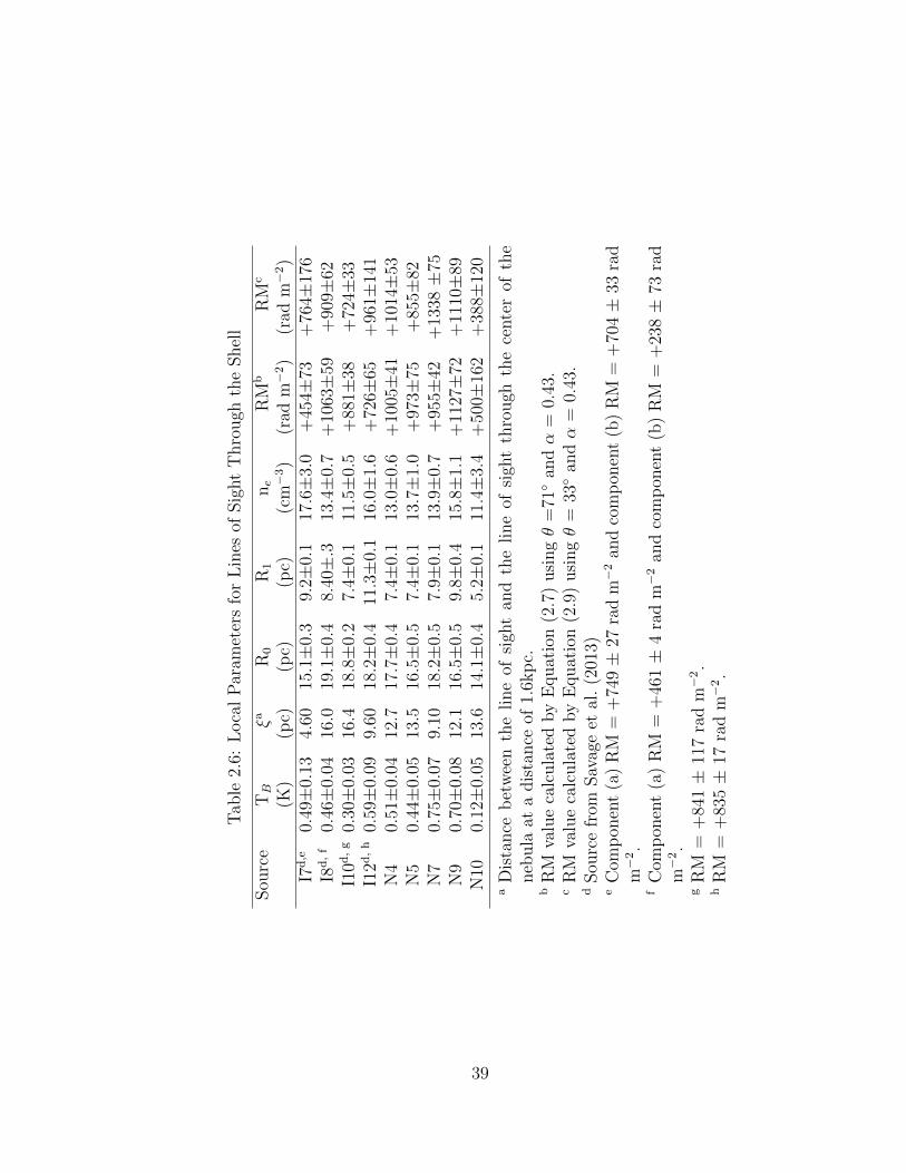
Tab

le2.

6:L

oca

lP

aram

eter

sfo

rL

ines

ofSig

ht

Thro

ugh

the

Shel

l

Sou

rce

TB

ξaR

0R

1ne

RM

bR

Mc

(K)

(pc)

(pc)

(pc)

(cm−

3)

(rad

m−

2)

(rad

m−

2)

I7d

,e0.

49±

0.13

4.60

15.1±

0.3

9.2±

0.1

17.6±

3.0

+45

4±73

+76

4±17

6I8

d,

f0.

46±

0.04

16.0

19.1±

0.4

8.40±

.313

.4±

0.7

+10

63±

59+

909±

62I1

0d,

g0.

30±

0.03

16.4

18.8±

0.2

7.4±

0.1

11.5±

0.5

+88

1±38

+72

4±33

I12d

,h

0.59±

0.09

9.60

18.2±

0.4

11.3±

0.1

16.0±

1.6

+72

6±65

+96

1±14

1N

40.

51±

0.04

12.7

17.7±

0.4

7.4±

0.1

13.0±

0.6

+10

05±

41+

1014±

53N

50.

44±

0.05

13.5

16.5±

0.5

7.4±

0.1

13.7±

1.0

+97

3±75

+85

5±82

N7

0.75±

0.07

9.10

18.2±

0.5

7.9±

0.1

13.9±

0.7

+95

5±42

+13

38±

75N

90.

70±

0.08

12.1

16.5±

0.5

9.8±

0.4

15.8±

1.1

+11

27±

72+

1110±

89N

100.

12±

0.05

13.6

14.1±

0.4

5.2±

0.1

11.4±

3.4

+50

0±16

2+

388±

120

aD

ista

nce

bet

wee

nth

eline

ofsi

ght

and

the

line

ofsi

ght

thro

ugh

the

cente

rof

the

neb

ula

ata

dis

tance

of1.

6kp

c.b

RM

valu

eca

lcula

ted

by

Equat

ion

(2.7

)usi

ngθ

=71

andα

=0.

43.

cR

Mva

lue

calc

ula

ted

by

Equat

ion

(2.9

)usi

ngθ

=33

andα

=0.

43.

dSou

rce

from

Sav

age

etal

.(2

013)

eC

omp

onen

t(a

)R

M=

+74

9±

27ra

dm−

2an

dco

mp

onen

t(b

)R

M=

+70

4±

33ra

dm−

2.

fC

omp

onen

t(a

)R

M=

+46

1±

4ra

dm−

2an

dco

mp

onen

t(b

)R

M=

+23

8±

73ra

dm−

2.

gR

M=

+84

1±

117

rad

m−

2.

hR

M=

+83

5±

17ra

dm−

2.

39

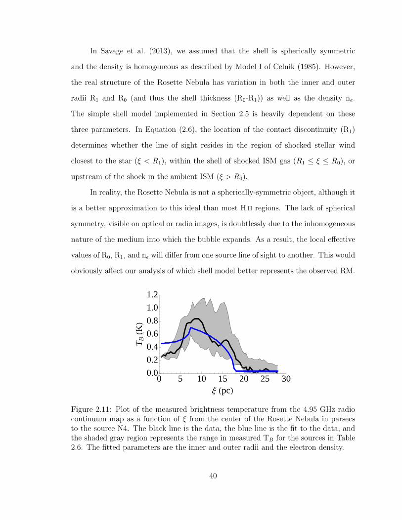
In Savage et al. (2013), we assumed that the shell is spherically symmetric

and the density is homogeneous as described by Model I of Celnik (1985). However,

the real structure of the Rosette Nebula has variation in both the inner and outer

radii R1 and R0 (and thus the shell thickness (R0-R1)) as well as the density ne.

The simple shell model implemented in Section 2.5 is heavily dependent on these

three parameters. In Equation (2.6), the location of the contact discontinuity (R1)

determines whether the line of sight resides in the region of shocked stellar wind

closest to the star (ξ < R1), within the shell of shocked ISM gas (R1 ≤ ξ ≤ R0), or

upstream of the shock in the ambient ISM (ξ > R0).

In reality, the Rosette Nebula is not a spherically-symmetric object, although it

is a better approximation to this ideal than most H ii regions. The lack of spherical

symmetry, visible on optical or radio images, is doubtlessly due to the inhomogeneous

nature of the medium into which the bubble expands. As a result, the local effective

values of R0, R1, and ne will differ from one source line of sight to another. This would

obviously affect our analysis of which shell model better represents the observed RM.

0 5 10 15 20 25 300.0

0.2

0.4

0.6

0.8

1.0

1.2

Ξ HpcL

TB

HKL

Figure 2.11: Plot of the measured brightness temperature from the 4.95 GHz radiocontinuum map as a function of ξ from the center of the Rosette Nebula in parsecsto the source N4. The black line is the data, the blue line is the fit to the data, andthe shaded gray region represents the range in measured TB for the sources in Table2.6. The fitted parameters are the inner and outer radii and the electron density.

40

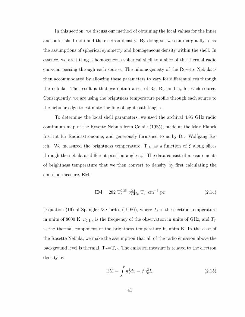
In this section, we discuss our method of obtaining the local values for the inner

and outer shell radii and the electron density. By doing so, we can marginally relax

the assumptions of spherical symmetry and homogeneous density within the shell. In

essence, we are fitting a homogeneous spherical shell to a slice of the thermal radio

emission passing through each source. The inhomogeneity of the Rosette Nebula is

then accommodated by allowing these parameters to vary for different slices through

the nebula. The result is that we obtain a set of R0, R1, and ne for each source.

Consequently, we are using the brightness temperature profile through each source to

the nebular edge to estimate the line-of-sight path length.

To determine the local shell parameters, we used the archival 4.95 GHz radio

continuum map of the Rosette Nebula from Celnik (1985), made at the Max Planck

Institut fur Radioastronomie, and generously furnished to us by Dr. Wolfgang Re-

ich. We measured the brightness temperature, TB, as a function of ξ along slices

through the nebula at different position angles ψ. The data consist of measurements

of brightness temperature that we then convert to density by first calculating the

emission measure, EM,

EM = 282 T0.358 ν2.1

GHz TT cm−6 pc (2.14)

(Equation (19) of Spangler & Cordes (1998)), where T8 is the electron temperature

in units of 8000 K, νGHz is the frequency of the observation in units of GHz, and TT

is the thermal component of the brightness temperature in units K. In the case of

the Rosette Nebula, we make the assumption that all of the radio emission above the

background level is thermal, TT=TB. The emission measure is related to the electron

density by

EM =

∫n2edz = fn2

eL, (2.15)

41

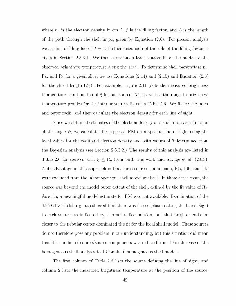
where ne is the electron density in cm−3, f is the filling factor, and L is the length

of the path through the shell in pc, given by Equation (2.6). For present analysis

we assume a filling factor f = 1; further discussion of the role of the filling factor is

given in Section 2.5.3.1. We then carry out a least-squares fit of the model to the

observed brightness temperature along the slice. To determine shell parameters ne,

R0, and R1 for a given slice, we use Equations (2.14) and (2.15) and Equation (2.6)

for the chord length L(ξ). For example, Figure 2.11 plots the measured brightness

temperature as a function of ξ for one source, N4, as well as the range in brightness

temperature profiles for the interior sources listed in Table 2.6. We fit for the inner

and outer radii, and then calculate the electron density for each line of sight.

Since we obtained estimates of the electron density and shell radii as a function

of the angle ψ, we calculate the expected RM on a specific line of sight using the

local values for the radii and electron density and with values of θ determined from

the Bayesian analysis (see Section 2.5.3.2.) The results of this analysis are listed in

Table 2.6 for sources with ξ ≤ R0 from both this work and Savage et al. (2013).

A disadvantage of this approach is that three source components, I6a, I6b, and I15

were excluded from the inhomogeneous shell model analysis. In these three cases, the

source was beyond the model outer extent of the shell, defined by the fit value of R0.

As such, a meaningful model estimate for RM was not available. Examination of the

4.95 GHz Effelsburg map showed that there was indeed plasma along the line of sight

to each source, as indicated by thermal radio emission, but that brighter emission

closer to the nebular center dominated the fit for the local shell model. These sources

do not therefore pose any problem in our understanding, but this situation did mean

that the number of source/source components was reduced from 19 in the case of the

homogeneous shell analysis to 16 for the inhomogeneous shell model.

The first column of Table 2.6 lists the source defining the line of sight, and

column 2 lists the measured brightness temperature at the position of the source.

42

The value of ξ for the source is listed in column 3. Columns 4, 5, and 6 list the

estimates of R0, R1, and ne, respectively. Finally, columns 7 and 8 give the calculated

RM values from Equations (2.7) and (2.9), respectively.

Figures 2.12a and 2.12b plot the observed RM vs the modeled RM values cal-

culated with Equations (2.7) and (2.9), respectively, for sources with ξ ≤ R0. The

line in these figures represents the case of perfect agreement between the observed

RM and calculated RM values. The errors for the modeled RM values are propagated

from the fits of TB, R0, and R1. For both cases, Figure 2.12a and Figure 2.12b, there

is rough agreement between observations and the model when the model predicts

intermediate RM, i.e., +400 ≤ RM ≤ +1000 rad m−2. When the models predict high

RM, however, the results are mixed. For some lines of sight, the observed RM are in

reasonable agreement with the model values. However, in other cases, the observed

RM is considerably lower.

It is unclear physically why this is the case. It is possible that some of these

lines of sight pass through regions in which B is strongly modified from the simplified

forms assumed in our analysis. In such cases, reversal of the shell magnetic field for

some portion of the line of sight could lead to a drop in the total RM. Alternatively,

it is possible that lines of sight characterized by low observed RM relative to model

predictions are probing plasma cavities within the shell. This possibility is rendered

less likely by the fact that the results of Figure 2.12 have taken into account the

emission measure along a slice at the same position angle ψ as the source. It has

been suggested to us (D. Schnitzeler, private communication) that these low RMs for

some lines of sight could indicate a low value of the filling factor f . This is more-

or-less equivalent to the above suggestion that the anomalously low RMs are due to

cavities in the nebula.

It is possible to have very high values of the RM that could potentially wrap

within the bandwidth, which may cause depolarization. However, we do not believe

43

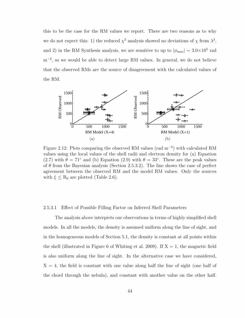
this to be the case for the RM values we report. There are two reasons as to why

we do not expect this: 1) the reduced χ2 analysis showed no deviations of χ from λ2,

and 2) in the RM Synthesis analysis, we are sensitive to up to |φmax| ∼ 3.0×105 rad

m−2, so we would be able to detect large RM values. In general, we do not believe

that the observed RMs are the source of disagreement with the calculated values of

the RM.

0 500 1000 15000

500

1000

1500

RM Model HX=4L

RM

Obse

rved

(a)

0 500 1000 15000

500

1000

1500

RM Model HX=1LR

MO

bse

rved

(b)

Figure 2.12: Plots comparing the observed RM values (rad m−2) with calculated RMvalues using the local values of the shell radii and electron density for (a) Equation(2.7) with θ = 71 and (b) Equation (2.9) with θ = 33. These are the peak valuesof θ from the Bayesian analysis (Section 2.5.3.2). The line shows the case of perfectagreement between the observed RM and the model RM values. Only the sourceswith ξ ≤ R0 are plotted (Table 2.6).

2.5.3.1 Effect of Possible Filling Factor on Inferred Shell Parameters

The analysis above interprets our observations in terms of highly simplified shell

models. In all the models, the density is assumed uniform along the line of sight, and

in the homogeneous models of Section 5.1, the density is constant at all points within

the shell (illustrated in Figure 6 of Whiting et al. 2009). If X = 1, the magnetic field

is also uniform along the line of sight. In the alternative case we have considered,

X = 4, the field is constant with one value along half the line of sight (one half of

the chord through the nebula), and constant with another value on the other half.

44

This homogeneity has been assumed in recognition of the patent oversimplification of

these models in describing the true H ii region associated with the Rosette Nebula.

Another parameter which frequently appears in the literature in discussions

of H ii regions is the filling factor f , conventionally defined as the fraction of the

H ii region volume that is occupied by ionized gas, as opposed to a vacuum which

allegedly occupies the remainder of the volume. Harvey-Smith et al. (2011) adopt a

value of f = 0.1 on the basis of numbers reported in the literature, and this value

is incorporated in their estimates of B‖. Purcell et al. (2015) adopted a value of

f = 0.3 for the Gum Nebula, but noted that it was poorly constrained, and could

be significantly larger. Planck Collaboration (2015), in their study of the Rosette

Nebula, assumed a value of f = 1, apparently in view of the absence of data indicating

a smaller number.

There are two ways of estimating the filling factor for an H ii region.

1. In the first investigation of this matter, Osterbrock & Flather (1959) measured

the density in the central part of the Orion Nebula from the density-sensitive line

ratio OII 3729/3726. They showed that the inferred density, if taken as uniform

through the nebula, would result in an EM much larger than that obtained

by measurement of the radio thermal continuum emission. The resolution,

illustrated in Figure 7 of Osterbrock & Flather (1959), was to posit that the

ionized gas was contained in clouds occupying a small fraction of the nebular

volume. This same approach, using density-sensitive infrared lines of SIII was

used by Herter et al. (1982) to reach similar conclusions about the H ii regions

G75.84+0.4 and W3 IRS 1. We were unable to find suitable measurements of

the OII 3729/3726 doublet in the Rosette Nebula, so an estimate of f in this

way could not be done.

2. A second method for determining the filling factor was presented in Kassim et al.

45

(1989). It relies solely on radio measurements and could be termed a radiometric

method of determining f . The estimate of f from Kassim et al. (1989) results

from requiring consistency between the optically thin radio flux of a nebula and

estimates of EM obtained from the low frequency radio spectrum, at and below

frequencies at which the nebula becomes optically thick (see Equations (6) and

(7) of Kassim et al. 1989). The filling factor is then defined as

f ≡ Ω

Ωbeam

(2.16)

where Ω is the inferred solid angle subtended by regions of emission, and Ωbeam

is the beam of the radio telescope, i.e. the solid angle over which all emission

is averaged.

An apparently equivalent (i.e. using the same physical concepts) formulation of the

Kassim et al. (1989) method compares the measured brightness temperature TB of

the H ii region in the optically thick part of the spectrum (more precisely, the an-

tenna temperature TA attributable to the thermal emission of the nebula) to the

independently-determined electron temperature Te,

f =Ω

Ωbeam

=TBTe. (2.17)

Equation (2.17), applied to the data of Kassim et al. (1989) on H ii regions associated

with the S53 complex, reproduces the filling factors in Table 5 of Kassim et al. (1989).

It should be noted that the filling factor calculated in the method of Kassim et al.

(1989) will not usually equal that defined by Osterbrock & Flather (1959), but should

indicate if the latter is substantially less than unity, and may be used as a rough

estimate in the absence of other information.

An estimate of f using the method of Kassim et al. (1989) is possible for the

46

Rosette Nebula. Graham et al. (1982) assembled radio continuum measurements of

the Rosette Nebula over a wide range of frequencies, and showed that the nebula

becomes optically thick at a frequency of about 400 MHz. From a fit to the lower

frequency part of the spectrum, they obtain an optically-thick brightness (antenna)

temperature of TB = 4100+700−500 K. Celnik (1986) reports an independent measurement

of the electron temperature Te, based on radio recombination line observations. Celnik

measures Te = 4700±600 K if LTE level populations are assumed, and Te = 5800±700

K on the basis of a non-LTE calculation. Adopting the latter value for Te, a value

of f = 0.71± 0.13 results. Given the uncertainty in this whole procedure, this value

should probably not be considered strongly inconsistent with f = 1.

We now briefly discuss the consequences of a filling factor f ∼ 0.7 on the analysis

presented in this paper. If f (now taken to be the fraction of line of sight occupied

by clumps containing plasma) is less than unity, the true density in those clumps

will be larger by a factor of 1/√f than deduced for a uniform shell. Likewise, the

value of B0z in the clumps will be larger by the same factor. Since our modeling

of RM observations constrains the quantity B0z = B0 cos θ (Equation (2.8)), the

consequences of f < 1 are given in the following expression,

B10 cos θ1

√f

= Bf0 cos θf (2.18)

with the variables defined as follows. The quantities B10 and θ1 are the magnetic field

strength and inclination angle in the case f = 1 (homogeneous shell). These are the

quantities presented in the previous sections. The variables Bf0 and θf represent the

corresponding quantities when f ≤ 1. If we assume that B10 = Bf

0 = B0 is known,

Equation (2.18) becomes an identity relating θ1 and θf .

Table 2.7 reports our results concerning the effects of a value of f less than

unity. This table presents values of θf corresponding to different values of f . Column

47

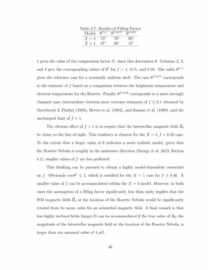
Table 2.7: Results of Filling FactorModel θf=1 θf=0.71 θf=0.5

X = 4 73 70 66

X = 1 47 36 15

1 gives the value of the compression factor X, since this determines θ. Columns 2, 3,

and 4 give the corresponding values of θf for f = 1, 0.71, and 0.50. The value θf=1

gives the reference case for a nominally uniform shell. The case θf=0.71 corresponds

to the estimate of f based on a comparison between the brightness temperature and

electron temperature for the Rosette. Finally, θf=0.50 corresponds to a more strongly

clumped case, intermediate between more extreme estimates of f ≤ 0.1 obtained by

Osterbrock & Flather (1959), Herter et al. (1982), and Kassim et al. (1989), and the

unclumped limit of f = 1.

The obvious effect of f < 1 is to require that the interstellar magnetic field ~B0

be closer to the line of sight. This tendency is clearest for the X = 1, f = 0.50 case.

To the extent that a larger value of θ indicates a more realistic model, given that

the Rosette Nebula is roughly in the anticenter direction (Savage et al. 2013, Section

4.1), smaller values of f are less preferred.

This thinking can be pursued to obtain a highly model-dependent constraint

on f . Obviously cos θf ≤ 1, which is satisfied for the X = 1 case for f ≥ 0.46. A

smaller value of f can be accommodated within the X = 4 model. However, in both

cases the assumption of a filling factor significantly less than unity implies that the

ISM magnetic field ~B0 at the location of the Rosette Nebula would be significantly

rotated from its mean value for an azimuthal magnetic field. A final remark is that

less highly inclined fields (larger θ) can be accommodated if the true value of B0, the

magnitude of the interstellar magnetic field at the location of the Rosette Nebula, is

larger than our assumed value of 4 µG.

48

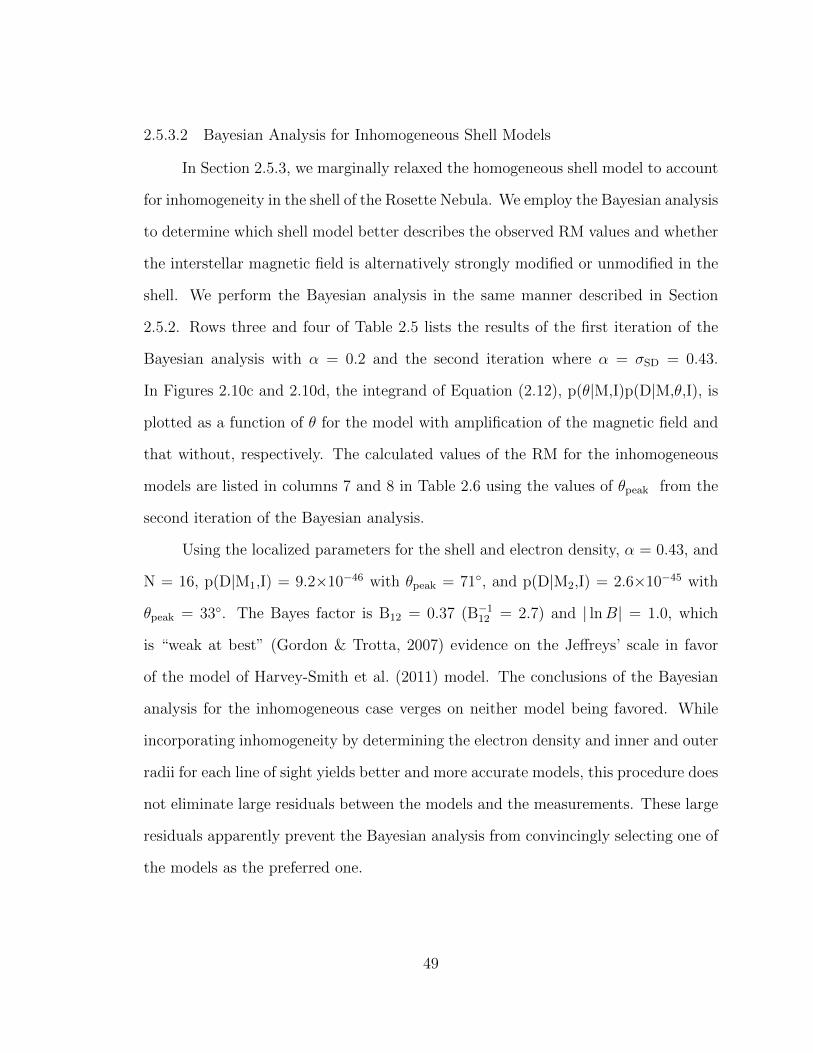
2.5.3.2 Bayesian Analysis for Inhomogeneous Shell Models

In Section 2.5.3, we marginally relaxed the homogeneous shell model to account

for inhomogeneity in the shell of the Rosette Nebula. We employ the Bayesian analysis

to determine which shell model better describes the observed RM values and whether

the interstellar magnetic field is alternatively strongly modified or unmodified in the

shell. We perform the Bayesian analysis in the same manner described in Section

2.5.2. Rows three and four of Table 2.5 lists the results of the first iteration of the

Bayesian analysis with α = 0.2 and the second iteration where α = σSD = 0.43.

In Figures 2.10c and 2.10d, the integrand of Equation (2.12), p(θ|M,I)p(D|M,θ,I), is

plotted as a function of θ for the model with amplification of the magnetic field and

that without, respectively. The calculated values of the RM for the inhomogeneous

models are listed in columns 7 and 8 in Table 2.6 using the values of θpeak from the

second iteration of the Bayesian analysis.

Using the localized parameters for the shell and electron density, α = 0.43, and

N = 16, p(D|M1,I) = 9.2×10−46 with θpeak = 71, and p(D|M2,I) = 2.6×10−45 with

θpeak = 33. The Bayes factor is B12 = 0.37 (B−112 = 2.7) and | lnB| = 1.0, which

is “weak at best” (Gordon & Trotta, 2007) evidence on the Jeffreys’ scale in favor

of the model of Harvey-Smith et al. (2011) model. The conclusions of the Bayesian

analysis for the inhomogeneous case verges on neither model being favored. While

incorporating inhomogeneity by determining the electron density and inner and outer

radii for each line of sight yields better and more accurate models, this procedure does

not eliminate large residuals between the models and the measurements. These large

residuals apparently prevent the Bayesian analysis from convincingly selecting one of

the models as the preferred one.

49

2.5.4 Summary of Bayesian Test of Models

The Bayesian analysis was undertaken to determine which of the simplified

models discussed in Section 2.5.1 is a better representation of the Rosette Nebula

Faraday rotation data. The results of the Bayesian analysis are listed in Table 2.5.

If a global shell model (i.e., the same values of R0, R1, and ne for all lines of sight)

is applied to the data, the Bayes factor is B12 = 0.19 (B−112 = 5.4) and | lnB| =

1.7, indicating that the picture of Harvey-Smith et al. (2011), i.e., a model without

modification of B0, is weakly favored in its ability to reproduce the observations

(Section 2.5.2).

If an attempt is made to accommodate the inhomogeneity of the nebula by

having the effective values of R0, R1, and ne change for different slices through the

nebula, the Bayes factor is B12 = 0.37 (B−112 = 2.7) and | lnB| = 1.0, which is “weak

at best” (Gordon & Trotta, 2007) in favor of the Harvey-Smith et al. (2011) model.

The results of the Bayesian analysis depend on the choice of α. This probably

is a consequence of the fact that as α increases, the role of outliers in the likelihood

function decreases. In any case, as the value of α is increased from 0.20 to 0.43, the

preferred inhomogeneous model changes from weakly in favor of the X=4 model to

weakly in favor of the X=1 (unmodified) model.

Our analysis is also sensitive to our choice of prior, i.e., allowing θ to range on

a surface of a hemisphere. This choice of prior can bias the results at higher values

of θ. We initially performed the Bayesian analysis with a uniform prior such that

p(θ|M, I) = 1∆θ, where ∆θ=π

2. However, the choice of prior does not change which

model is favored in the Bayesian analysis.

The conclusions of the Bayesian analysis are not strong, and the inability of

this analysis to identify a clear preferred model is apparently due to the oversimplified

nature of all models considered. Inhomogeneities or other structures in the real nebula

50

partially mask the average properties of the nebula. However, a positive point is that

either model can reproduce the magnitude and extent of enhanced RMs over the right

angular extent on the sky, for plausible values of the magnitude and orientation of

the interstellar magnetic field. For the global models, which predict that the RM

should depend only on the impact parameter ξ, the plot to consult is Figure 2.9.

Both models account for the abrupt onset of the RM at the edge of the nebula, and

both reproduce, with plausible values of the independent parameter θ, the values of

RM actually observed. However, an equally striking aspect of Figure 2.9 is the large

dispersion of measured RMs about the model curves. Apparently, variations in the

plasma structure of the stellar bubble, describable by variations in ne, |B|, and θ are

as important as the description of the mean shell characteristics, and in fact obscure

the signature of this mean structure.

For the case of the “inhomogeneous models”, the relevant plot is Figure 2.12. In

the inhomogeneous case, the predicted RM does not depend only on ξ, and we make

a comparison between the model and observable values for all lines of sight. Here,

again, the models meet with some success in that they can reproduce the magnitude

of the RMs observed, and are also able to partially account for the variation of RM

from one line of sight to another. That is, the models seem to successfully predict

the upper envelope of the observed RMs. However, the models do not account for

the fact that some lines of sight, expected to have large RMs, have intermediate to

low values. Again we must appeal to spatial variations within the nebula, potentially

describable as large-scale turbulence, that cause variations in the values of RM.

As a final comment, it is worthwhile to know that plausible variations in one

parameter, θ, allow two models that significantly differ in a physical sense to rea-

sonably account for the data. We suspect that this statement would extend to the

model presented by Planck Collaboration et al. (2015). Their physical description of

the nebular shell is very different and probably more realistic than those considered

51

in this paper. Their result for the prediction of RM(ξ), presented in Figure 6 of their

paper, is similar in form to that shown in Figure 2.9 of our paper, with different but

plausible values of |B0| and θ. However, it is not capable of accounting for substantial

dispersion in RM for lines of sight with the same value of ξ.

2.6 Summary and Conclusions

1. We performed polarimetric observations using the VLA of 11 new radio sources

observed through the shell of the Rosette Nebula. This significantly increases

the number of lines of sight probed relative to that of Savage et al. (2013).

2. We obtained RM measurements for 15 lines of sight (including secondary com-

ponents), using two techniques: a least-squares fit to χ(λ2) and RM Synthesis.

The measured RM values are in excellent agreement between the two techniques.

We measure an excess RM of +40 to +1200 rad m−2 due to the shell of the

Rosette Nebula and confirm the background RM of +147 rad m−2 from Savage

et al. (2013). The large range in values of RM through the shell is an indicator

of inhomogeneity in the shell, which is beyond the scope of the present paper.

3. We employ a Bayesian analysis to determine which of two models better rep-

resents the observed dependence of RM with distance from the center of the

nebula, a model with a shock-enhanced magnetic field in the shell or one with-

out. We first treat the Rosette Nebula as a spherically-symmetric shell having

global parameters for the inner and outer radii of the shell and the electron den-

sity. With this calculation, the model without modification of the interstellar

field is favored. The Bayes factor is 5.4 (B12−1) and on the Jeffreys’ scale, the

analysis of Harvey-Smith et al. (2011) is weakly favored.

4. We perform a second Bayesian analysis using localized parameters determined

from radio continuum data to account for the inhomogeneity of the shell. In

52

this analysis, we model the inner and outer shell radii and calculate the electron

density to each line of sight. We then employ these localized parameters in the

Bayesian analysis and find the model without modification of the magnetic field

in the shell is weakly favored. The Bayes factor is 2.7, which on the Jeffreys’

scale (| ln B| = 1.0) is considered “weak at best” (Gordon & Trotta, 2007).

5. The results of the Bayesian analysis are dependent on the value of α, which

specifies the expected departure of the measurements from the model. For a

value of α ' 0.4, neither model is significantly superior to the other in a Bayesian

sense. We attribute this to the fact that neither model can account for large

departures of the observed RMs from the model predictions. This situation is

unlikely to change, even for analytic and numerical models that include more

sophisticated physics than the empirical expressions we have employed.

6. Regardless of the specific choice of model, the magnitude and spatial extent

of the rotation measure “anomaly” is completely consistent with independent

information on the plasma density in the nebula, and the interstellar magnetic

field.

7. To further investigate the role of magnetic fields in H ii regions, one would want

more lines of sight through the shell of the Rosette H ii region and the stellar

bubble to obtain a large sample of RM values. In many cases though, such

a sample is limited by the number of strong, linearly polarized, extragalactic

sources behind the nebula. Simulations of H ii regions and stellar bubbles with

magnetic fields, such as those by Stil et al. (2009), van Marle et al. (2015),

Ferriere et al. (1991), and Walch et al. (2015), are vital to understanding how

the magnetic field and the density contribute to the large RM values within the

shell of the nebula. It would be of considerable interest to compare calculated

RMs on lines of sight through these simulations with the measured values. Such

53

comparison would indicate if those simulations are capable of reproducing the

average features of Faraday rotation through these “Faraday Rotation Anoma-

lies” (Whiting et al., 2009), as well as the large fluctuations in the observed RMs

with respect to the expected values. Finally, similar analyses with more H ii

regions and stellar bubbles would further illuminate the role of the magnetic

field and would allow one to consider differences in stellar composition, wind

luminosities, and ages of the nebulae. Presently, we are undertaking such an

analysis as presented in this paper for W4/IC 1805 and IC 1396.

54

CHAPTER 3

A FARADAY ROTATION STUDY OF THE STELLAR BUBBLE AND

H ii REGION ASSOCIATED WITH THE W4 COMPLEX

This chapter is taken directly from Costa & Spangler (2018), which has been

submitted to the Astrophysical Journal.

3.1 Introduction

Young massive stars in OB associations photoionize the surrounding gas, cre-

ating an H ii region, and their powerful stellar winds can inflate a bubble around

the star cluster. Magnetic fields are important to the dynamics of these structures

(Tomisaka, 1990; Ferriere et al., 1991; Vallee, 1993; Tomisaka, 1998; Haverkorn et al.,

2004; Sun et al., 2008; Stil et al., 2009), and they can elongate the cavity preferen-

tially in the direction of the magnetic field and thicken the shell perpendicular to the

field (Ferriere et al., 1991; de Avillez & Breitschwerdt, 2005; Stil et al., 2009), causing

deviations from the classical structure of the Weaver et al. (1977) wind-blown bubble.

Knowledge of the magnitude and direction of the magnetic field within stellar bubbles

and H ii regions is important for simulations and for understanding how the magnetic

field interacts with and modifies these structures.

In previous work (i.e., Savage et al. 2013 and Costa et al. 2016), we investigated

whether the Galactic magnetic field is amplified in the shell of the Rosette Nebula, an

H ii region and stellar bubble associated with NGC 2244 (` = 206.5, b = -2.1). In

this work, we continue our investigation of how H ii regions and stellar bubbles modify

the ambient Galactic magnetic field by considering another example of a young star

cluster and an H ii region that appears to be formed into a shell by the effect of stellar

winds.

55

3.1.1 Techniques for Measuring Magnetic Fields in the Interstellar Medium

Faraday rotation measurements probe the line of sight (LOS) component of the

magnetic field in ionized parts of the interstellar medium (ISM), provided there is

an independent estimate of the electron density. Faraday rotation is the rotation in

the plane of polarization of a wave as it passes through magnetized plasma and is

described by the equation

χ = χ0 +

[(e3

2πm2ec

4

)∫ne B · ds

]λ2, (3.1)

where χ is the polarization position angle, χ0 is the intrinsic polarization position

angle, the quantities in the parentheses are the usual standard physical constants

in cgs units, ne is the electron density, B is the vector magnetic field, ds is the

incremental path length interval along the LOS, and λ is the wavelength. We define

the terms in the square bracket as the rotation measure, RM, and we can express the

RM in mixed but convenient interstellar units as

RM = 0.81

∫ne (cm−3) B (µG) · ds (pc) rad m−2. (3.2)

3.1.2 The H ii Region and Stellar Bubble Associated with the W4 Complex

The H ii region and stellar bubble of interest for the present study is IC 1805,

which is located in the Perseus Arm. The star cluster responsible for the H ii region

and stellar bubble is OCl 352, which is a young cluster (1–3 Myr) (Basu et al., 1999).

OCl 352 has 60 OB stars (Shi & Hu, 1999). Three of these are the O stars HD

15570, HD 15558, and HD 15629, and they have mass loss rates between 10−6 and

10−5 M yr−1 (Massey et al., 1995) and terminal wind velocities of 2200 – 3000 km

56

s−1 (Garmany, 1988; Groenewegen et al., 1989; Bouret et al., 2012). We adopt the

nominal center of the star cluster to be R.A.(J2000) = 02h 23m 42s, decl.(J2000) =

+6127′ 0′′ (` = 134.73, b = +0.92) (Guetter & Vrba, 1989) and a distance of 2.2 kpc

to IC 1805 to conform with previous studies of the region (e.g., Normandeau et al.

1996; Dennison et al. 1997; Reynolds et al. 2001; Terebey et al. 2003; Gao et al. 2015).

In the literature, other distance values include: 2.35 kpc (Massey et al., 1995; Basu

et al., 1999; West et al., 2007; Lagrois et al., 2012), 2 kpc (Dickel, 1980), 2.04 kpc

(Feigelson et al., 2013; Townsley et al., 2014), and 2.4 ± 0.1 kpc (Guetter & Vrba,

1989).

We refer to the H ii region between –0.2 < b < 2 as IC 1805. This structure

is also known as the Heart Nebula for its appearance at optical wavelengths. We

differentiate this region from the northern latitudes that constitute the W4 Super-

bubble (Normandeau et al., 1996; West et al., 2007; Gao et al., 2015), and we use the

nomenclature of W4 to describe the entire region, which includes IC 1805 and the

W4 Superbubble. Below we summarize the structure of IC 1805 and Figure 3.1 is a

cartoon diagram of the structure described here.

– South. On the southern portion of IC 1805, there is a loop structure of ionized

material at 134< ` < 136, b < 1, which we call the southern loop. Terebey

et al. (2003) find that at far infrared and radio wavelengths, the shell structure

is well defined and ionization bounded, since the ionized gas lies interior to

the dust shell. However, they also find that there is warm dust that extends

past the southern loop and a faint ionized halo (see their Figure 6). Terebey

et al. (2003) argue that the shell is patchy and inhomogeneous in density, which

allows ionizing photons to escape. Gray et al. (1999) discuss extended emission

surrounding IC 1805 and suggest that it may be evidence of an extended H ii

region (Anantharamaiah, 1985). Also surrounding IC 1805 are patchy regions

of H i (Braunsfurth, 1983; Hasegawa et al., 1983; Sato, 1990) and CO (Heyer &

57

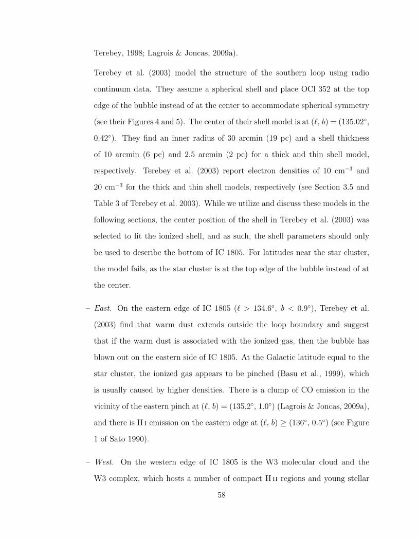
Terebey, 1998; Lagrois & Joncas, 2009a).

Terebey et al. (2003) model the structure of the southern loop using radio

continuum data. They assume a spherical shell and place OCl 352 at the top

edge of the bubble instead of at the center to accommodate spherical symmetry

(see their Figures 4 and 5). The center of their shell model is at (`, b) = (135.02,

0.42). They find an inner radius of 30 arcmin (19 pc) and a shell thickness

of 10 arcmin (6 pc) and 2.5 arcmin (2 pc) for a thick and thin shell model,

respectively. Terebey et al. (2003) report electron densities of 10 cm−3 and

20 cm−3 for the thick and thin shell models, respectively (see Section 3.5 and

Table 3 of Terebey et al. 2003). While we utilize and discuss these models in the

following sections, the center position of the shell in Terebey et al. (2003) was

selected to fit the ionized shell, and as such, the shell parameters should only

be used to describe the bottom of IC 1805. For latitudes near the star cluster,

the model fails, as the star cluster is at the top edge of the bubble instead of at

the center.

– East. On the eastern edge of IC 1805 (` > 134.6, b < 0.9), Terebey et al.

(2003) find that warm dust extends outside the loop boundary and suggest

that if the warm dust is associated with the ionized gas, then the bubble has

blown out on the eastern side of IC 1805. At the Galactic latitude equal to the

star cluster, the ionized gas appears to be pinched (Basu et al., 1999), which

is usually caused by higher densities. There is a clump of CO emission in the

vicinity of the eastern pinch at (`, b) = (135.2, 1.0) (Lagrois & Joncas, 2009a),

and there is H i emission on the eastern edge at (`, b) ≥ (136, 0.5) (see Figure

1 of Sato 1990).

– West. On the western edge of IC 1805 is the W3 molecular cloud and the

W3 complex, which hosts a number of compact H ii regions and young stellar

58

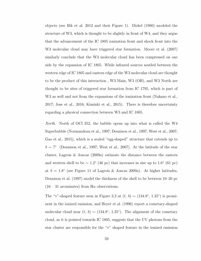
objects (see Bik et al. 2012 and their Figure 1). Dickel (1980) modeled the

structure of W3, which is thought to be slightly in front of W4, and they argue

that the advancement of the IC 1805 ionization front and shock front into the

W3 molecular cloud may have triggered star formation. Moore et al. (2007)

similarly conclude that the W3 molecular cloud has been compressed on one

side by the expansion of IC 1805. While infrared sources nestled between the

western edge of IC 1805 and eastern edge of the W3 molecular cloud are thought

to be the product of this interaction , W3 Main, W3 (OH), and W3 North are

thought to be sites of triggered star formation from IC 1795, which is part of

W3 as well and not from the expansions of the ionization front (Nakano et al.,

2017; Jose et al., 2016; Kiminki et al., 2015). There is therefore uncertainty

regarding a physical connection between W3 and IC 1805.

– North. North of OCl 352, the bubble opens up into what is called the W4

Superbubble (Normandeau et al., 1997; Dennison et al., 1997; West et al., 2007;

Gao et al., 2015), which is a sealed “egg-shaped” structure that extends up to

b ∼ 7 (Dennison et al., 1997; West et al., 2007). At the latitude of the star

cluster, Lagrois & Joncas (2009a) estimate the distance between the eastern

and western shell to be ∼ 1.2 (46 pc) that increases in size up to 1.6 (61 pc)

at b = 1.8 (see Figure 11 of Lagrois & Joncas 2009a). At higher latitudes,

Dennison et al. (1997) model the thickness of the shell to be between 10–20 pc

(16 – 31 arcminutes) from Hα observations.

The “v”-shaped feature seen in Figure 3.2 at (`, b) ∼ (134.8, 1.35) is promi-

nent in the ionized emission, and Heyer et al. (1996) report a cometary-shaped

molecular cloud near (`, b) ∼ (134.8, 1.35). The alignment of the cometary

cloud, as it is pointed towards IC 1805, suggests that the UV photons from the

star cluster are responsible for the “v” shaped feature in the ionized emission

59

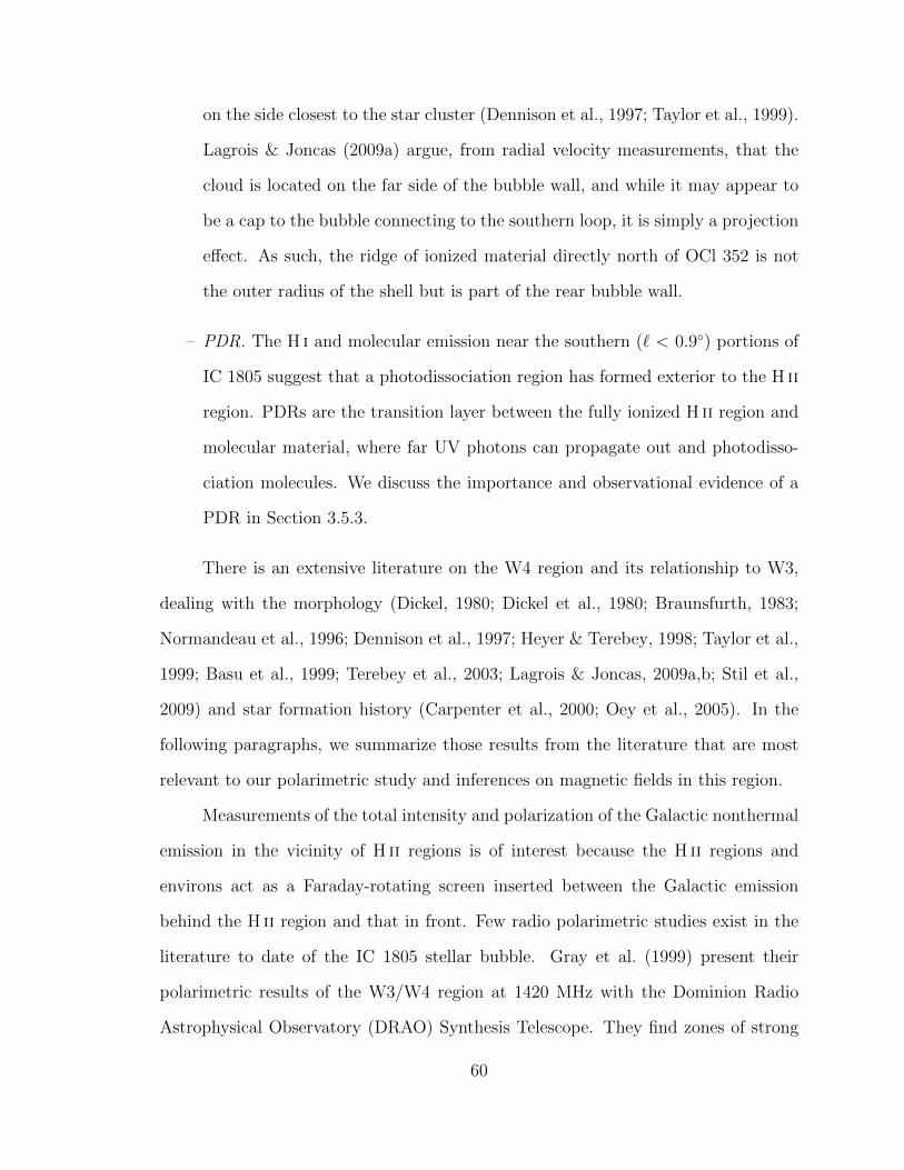
on the side closest to the star cluster (Dennison et al., 1997; Taylor et al., 1999).

Lagrois & Joncas (2009a) argue, from radial velocity measurements, that the

cloud is located on the far side of the bubble wall, and while it may appear to

be a cap to the bubble connecting to the southern loop, it is simply a projection

effect. As such, the ridge of ionized material directly north of OCl 352 is not

the outer radius of the shell but is part of the rear bubble wall.

– PDR. The H i and molecular emission near the southern (` < 0.9) portions of

IC 1805 suggest that a photodissociation region has formed exterior to the H ii

region. PDRs are the transition layer between the fully ionized H ii region and

molecular material, where far UV photons can propagate out and photodisso-

ciation molecules. We discuss the importance and observational evidence of a

PDR in Section 3.5.3.

There is an extensive literature on the W4 region and its relationship to W3,

dealing with the morphology (Dickel, 1980; Dickel et al., 1980; Braunsfurth, 1983;

Normandeau et al., 1996; Dennison et al., 1997; Heyer & Terebey, 1998; Taylor et al.,

1999; Basu et al., 1999; Terebey et al., 2003; Lagrois & Joncas, 2009a,b; Stil et al.,

2009) and star formation history (Carpenter et al., 2000; Oey et al., 2005). In the

following paragraphs, we summarize those results from the literature that are most

relevant to our polarimetric study and inferences on magnetic fields in this region.

Measurements of the total intensity and polarization of the Galactic nonthermal

emission in the vicinity of H ii regions is of interest because the H ii regions and

environs act as a Faraday-rotating screen inserted between the Galactic emission

behind the H ii region and that in front. Few radio polarimetric studies exist in the

literature to date of the IC 1805 stellar bubble. Gray et al. (1999) present their

polarimetric results of the W3/W4 region at 1420 MHz with the Dominion Radio

Astrophysical Observatory (DRAO) Synthesis Telescope. They find zones of strong

60

Figure 3.1: Cartoon of structure of IC 1805 and the surrounding region, which includesthe W3 molecular cloud, W3 (blue filled circle), and the W4 Superbubble. The solidblack lines represent the bright ionized shell in Figure 3.2, the dotted lines showmolecular material from Lagrois & Joncas (2009a), and the gray shading representsthe extended halo or PDR. The star represents the center of the exciting star cluster,OCl 352.

depolarization near the H ii regions, particularly in the south, where there is a halo

of extended emission around IC 1805. They conclude that RM values on order 103

rad m−2 and spatial RM gradients must exist to explain the depolarization near the

H ii region. More recently, Hill et al. (2017) present results of their polarimetric

study of the Fan region (` ∼ 130, –5≤ b ≤ +10), which is a large structure in the

Perseus arm that includes W3/W4. While the focus of their study was not on W4

specifically, they find similar results to Gray et al. (1999) in that there is sufficient

Faraday rotation to cause beam depolarization in the regions of extended emission.

In the W4 Superbubble, West et al. (2007) determined the LOS magnetic field

strength by estimating depolarization effects along adjacent lines of sight. Using

estimates of the shell thickness and the electron density from Dennison et al. (1997),

61

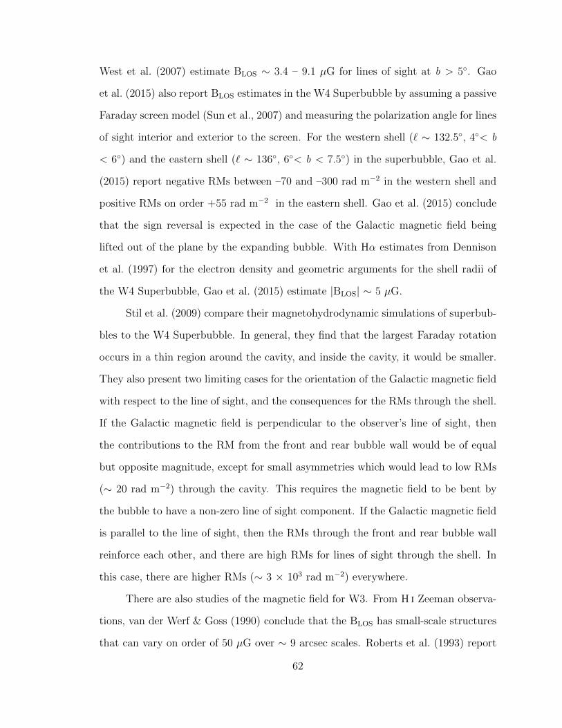
West et al. (2007) estimate BLOS ∼ 3.4 – 9.1 µG for lines of sight at b > 5. Gao

et al. (2015) also report BLOS estimates in the W4 Superbubble by assuming a passive

Faraday screen model (Sun et al., 2007) and measuring the polarization angle for lines

of sight interior and exterior to the screen. For the western shell (` ∼ 132.5, 4< b

< 6) and the eastern shell (` ∼ 136, 6< b < 7.5) in the superbubble, Gao et al.

(2015) report negative RMs between –70 and –300 rad m−2 in the western shell and

positive RMs on order +55 rad m−2 in the eastern shell. Gao et al. (2015) conclude

that the sign reversal is expected in the case of the Galactic magnetic field being

lifted out of the plane by the expanding bubble. With Hα estimates from Dennison

et al. (1997) for the electron density and geometric arguments for the shell radii of

the W4 Superbubble, Gao et al. (2015) estimate |BLOS| ∼ 5 µG.

Stil et al. (2009) compare their magnetohydrodynamic simulations of superbub-

bles to the W4 Superbubble. In general, they find that the largest Faraday rotation

occurs in a thin region around the cavity, and inside the cavity, it would be smaller.

They also present two limiting cases for the orientation of the Galactic magnetic field

with respect to the line of sight, and the consequences for the RMs through the shell.

If the Galactic magnetic field is perpendicular to the observer’s line of sight, then

the contributions to the RM from the front and rear bubble wall would be of equal

but opposite magnitude, except for small asymmetries which would lead to low RMs

(∼ 20 rad m−2) through the cavity. This requires the magnetic field to be bent by

the bubble to have a non-zero line of sight component. If the Galactic magnetic field

is parallel to the line of sight, then the RMs through the front and rear bubble wall

reinforce each other, and there are high RMs for lines of sight through the shell. In

this case, there are higher RMs (∼ 3 × 103 rad m−2) everywhere.

There are also studies of the magnetic field for W3. From H i Zeeman observa-

tions, van der Werf & Goss (1990) conclude that the BLOS has small-scale structures

that can vary on order of 50 µG over ∼ 9 arcsec scales. Roberts et al. (1993) report

62

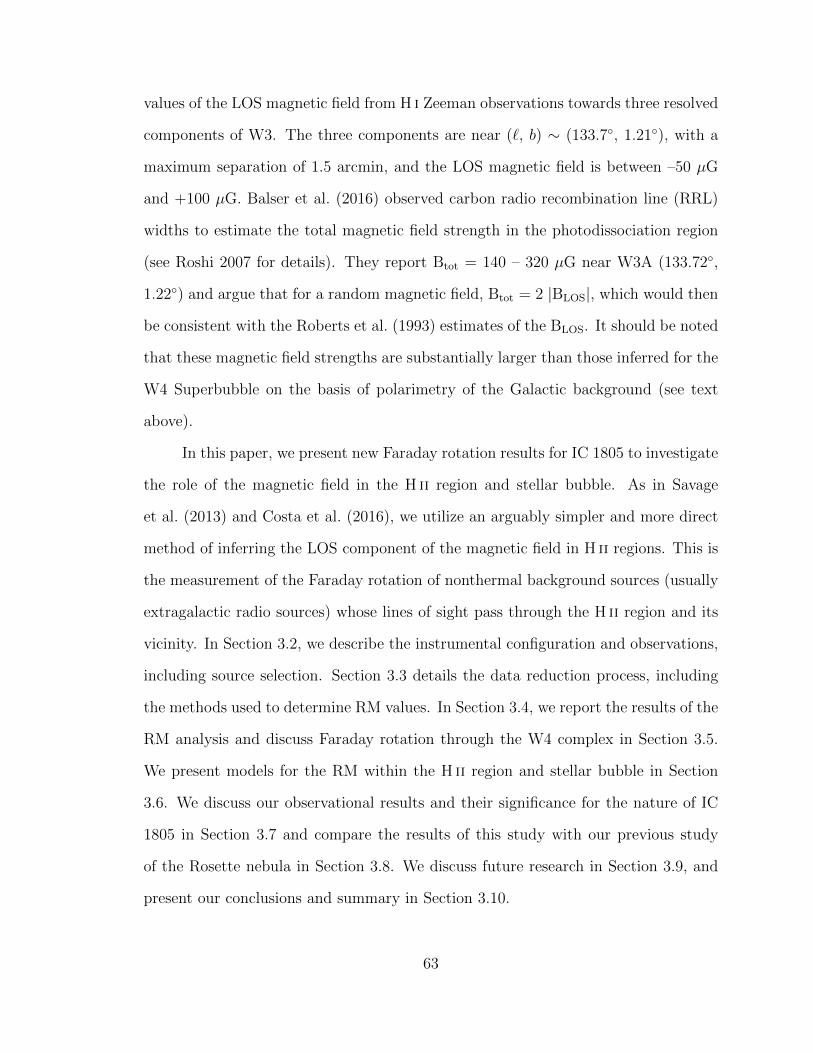
values of the LOS magnetic field from H i Zeeman observations towards three resolved

components of W3. The three components are near (`, b) ∼ (133.7, 1.21), with a

maximum separation of 1.5 arcmin, and the LOS magnetic field is between –50 µG

and +100 µG. Balser et al. (2016) observed carbon radio recombination line (RRL)

widths to estimate the total magnetic field strength in the photodissociation region

(see Roshi 2007 for details). They report Btot = 140 – 320 µG near W3A (133.72,

1.22) and argue that for a random magnetic field, Btot = 2 |BLOS|, which would then

be consistent with the Roberts et al. (1993) estimates of the BLOS. It should be noted

that these magnetic field strengths are substantially larger than those inferred for the

W4 Superbubble on the basis of polarimetry of the Galactic background (see text

above).

In this paper, we present new Faraday rotation results for IC 1805 to investigate

the role of the magnetic field in the H ii region and stellar bubble. As in Savage

et al. (2013) and Costa et al. (2016), we utilize an arguably simpler and more direct

method of inferring the LOS component of the magnetic field in H ii regions. This is

the measurement of the Faraday rotation of nonthermal background sources (usually

extragalactic radio sources) whose lines of sight pass through the H ii region and its

vicinity. In Section 3.2, we describe the instrumental configuration and observations,

including source selection. Section 3.3 details the data reduction process, including

the methods used to determine RM values. In Section 3.4, we report the results of the

RM analysis and discuss Faraday rotation through the W4 complex in Section 3.5.

We present models for the RM within the H ii region and stellar bubble in Section

3.6. We discuss our observational results and their significance for the nature of IC

1805 in Section 3.7 and compare the results of this study with our previous study

of the Rosette nebula in Section 3.8. We discuss future research in Section 3.9, and

present our conclusions and summary in Section 3.10.

63

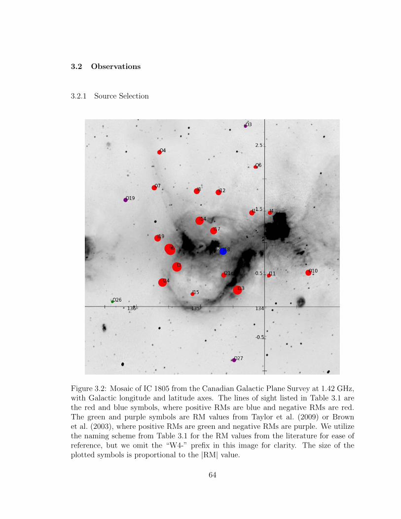
3.2 Observations

3.2.1 Source Selection

Figure 3.2: Mosaic of IC 1805 from the Canadian Galactic Plane Survey at 1.42 GHz,with Galactic longitude and latitude axes. The lines of sight listed in Table 3.1 arethe red and blue symbols, where positive RMs are blue and negative RMs are red.The green and purple symbols are RM values from Taylor et al. (2009) or Brownet al. (2003), where positive RMs are green and negative RMs are purple. We utilizethe naming scheme from Table 3.1 for the RM values from the literature for ease ofreference, but we omit the “W4-” prefix in this image for clarity. The size of theplotted symbols is proportional to the |RM| value.

64

Our criteria for source selection were identical to Savage et al. (2013) and Costa

et al. (2016) in that we searched the National Radio Astronomy Observatory Very

Large Array Sky Survey (NVSS, Condon et al. 1998) database for point sources

within 1 of OCl 352 (the “I” sources) with a minimum flux density of 20 mJy. We

also searched in an annulus centered on the star cluster with inner and outer radii

of 1 and 2 for outer sources (“O”) to measure the background RM due to the

general ISM. We identified 31 inner sources and 26 outer sources in the region. We

then inspected the NVSS postage stamps to ensure that they were point sources at

the resolution of the NVSS (∼ 45 arcseconds). We discarded sources that showed

extended structure similar to Galactic sources. We selected 24 inner sources and 8

outer sources from this final list.

The sources are listed in Table 3.1, where the first column lists the source name

in our nomenclature. The second and third columns list the right ascension (α)

and declination (δ) of the observed sources. The positions are determined with the

imfit task in CASA, which fits a 2D Gaussian to the intensity distribution at 4.33

GHz. Columns four and five give the Galactic longitude (`), Galactic latitude (b),

which is converted from α and δ using the Python Astropy package, and the angular

separation from the center of the nebula (ξ) is given in column six. Column seven

lists the flux density at 4.33 GHz calculated with imfit, and column eight gives the

mean percent linear polarization (m = P/I ) as measured across the eight 128 MHz

maps and assuming a Faraday simple source. Figure 3.2 is a radio continuum mosaic

from the Canadian Galactic Plane Survey (CGPS) (Taylor et al., 2003; Landecker

et al., 2010) with the location of the sources, along with the names, indicated with

filled circles.

65

Table 3.1: List of Sources ObservedSource α(J2000) δ(J2000) l b ξa S4.33GHz mName h m s o ′ ′′ (o) (o) (arcmin) (mJy) (%)

W4-I1 02 30 16.2 +62 09 37.9 134.19 1.47 46.0 77 4W4-I2 02 38 34.2 +61 08 46.6 135.49 0.91 46.2 5 12W4-I3 02 36 45.5 +60 55 48.8 135.38 0.63 42.8 82 3W4-I4 02 27 59.8 +62 15 44.0 133.91 1.47 58.9 46 10W4-I5b 02 28 01.6 +62 02 16.7 133.99 1.26 48.4 — —W4-I6 02 38 19.9 +61 08 03.5 135.47 0.89 44.8 12 11W4-I7b 02 27 33.8 +61 55 58.1 133.98 1.14 46.6 – —W4-I8 02 38 10.1 +62 08 57.0 135.05 1.81 57.1 47 9W4-I9 02 28 21.6 +61 28 36.5 134.23 0.75 31.1 — —W4-I10b 02 29 13.0 +61 00 53.4 134.50 0.36 36.2 — —W4-I11 02 25 15.2 +61 19 14.4 133.94 0.47 54.0 39 3W4-I12 02 35 20.6 +62 16 02.3 134.70 1.79 52.5 77 2W4-I13 02 28 25.1 +60 56 20.2 134.44 0.25 43.5 16 6W4-I14 02 36 19.2 +61 44 05.5 135.01 1.35 31.4 2 16W4-I15 02 33 36.1 +60 37 40.4 135.14 0.20 49.8 27 4W4-I16 02 36 56.8 +61 57 58.6 134.99 1.59 43.3 35 0W4-I17 02 34 08.8 +61 40 35.5 134.80 1.19 17.1 9 16W4-I18 02 31 56.3 +61 25 50.9 134.65 0.87 5.6 24 2W4-I19c 02 40 31.7 +61 13 45.9 135.68 1.09 57.8 11 3W4-I20 02 27 03.9 +61 52 24.9 133.94 1.07 47.6 457 0W4-I21 02 30 44.5 +61 05 30.2 134.64 0.50 25.9 5 7W4-I22b 02 26 07.8 +61 56 43.7 133.82 1.09 55.4 — —W4-I23 02 40 30.9 +61 47 10.1 135.45 1.59 59.3 3 0W4-I24 02 37 45.1 +60 37 31.4 135.61 0.40 61.5 20 10W4-O1 02 41 33.9 +61 26 29.5 135.70 1.33 63.5 377 0W4-O2 02 35 37.8 +59 56 29.5 135.64 -0.33 93.0 107 0W4-O4 02 44 57.7 +62 28 06.5 135.64 2.43 105.8 747 0W4-O5 02 21 52.6 +60 10 03.2 133.96 -0.75 110.3 94 0W4-O6 02 31 59.2 +62 50 34.1 134.12 2.18 83.7 120 4W4-O7 02 43 35.6 +61 55 54.6 135.72 1.88 82.7 52 0W4-O8 02 23 04.5 +60 58 19.6 133.82 0.05 75.2 40 0W4-O10 02 20 26.2 +61 34 46.2 133.31 0.51 88.0 64 3

a Angular distance between the line of sight and a line of sight through the centerof the star cluster.

b NVSS position. No source detected in the Stokes I map in any frequency bin.c High Mass X-Ray Binary LSI +61303.

66

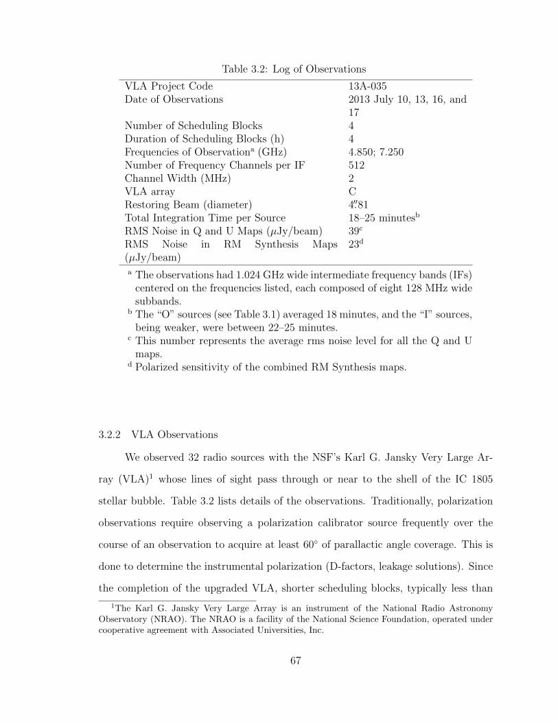
Table 3.2: Log of Observations

VLA Project Code 13A-035Date of Observations 2013 July 10, 13, 16, and

17Number of Scheduling Blocks 4Duration of Scheduling Blocks (h) 4Frequencies of Observationa (GHz) 4.850; 7.250Number of Frequency Channels per IF 512Channel Width (MHz) 2VLA array CRestoring Beam (diameter) 4.′′81Total Integration Time per Source 18–25 minutesb

RMS Noise in Q and U Maps (µJy/beam) 39c

RMS Noise in RM Synthesis Maps(µJy/beam)

23d

a The observations had 1.024 GHz wide intermediate frequency bands (IFs)centered on the frequencies listed, each composed of eight 128 MHz widesubbands.

b The “O” sources (see Table 3.1) averaged 18 minutes, and the “I” sources,being weaker, were between 22–25 minutes.

c This number represents the average rms noise level for all the Q and Umaps.

d Polarized sensitivity of the combined RM Synthesis maps.

3.2.2 VLA Observations

We observed 32 radio sources with the NSF’s Karl G. Jansky Very Large Ar-

ray (VLA)1 whose lines of sight pass through or near to the shell of the IC 1805

stellar bubble. Table 3.2 lists details of the observations. Traditionally, polarization

observations require observing a polarization calibrator source frequently over the

course of an observation to acquire at least 60 of parallactic angle coverage. This is

done to determine the instrumental polarization (D-factors, leakage solutions). Since

the completion of the upgraded VLA, shorter scheduling blocks, typically less than

1The Karl G. Jansky Very Large Array is an instrument of the National Radio AstronomyObservatory (NRAO). The NRAO is a facility of the National Science Foundation, operated undercooperative agreement with Associated Universities, Inc.

67

4 hours in duration, have become a common mode of observation. It is difficult, if

not impossible, with very short scheduling blocks to acquire enough parallactic angle

coverage to measure the instrumental calibration with a polarized source. Another

method of determining the instrumental polarization is to observe a single scan of an

unpolarized source. This technique can be used with shorter scheduling blocks.

In this project we calibrated the instrumental polarization using both tech-

niques. We used the source J0228+6721, observed over a wide range of parallactic

angle, and also made a single scan of the unpolarized source 3C84. Use of the CASA

task polcal on the J0228+6721 data solved for the instrumental polarization, deter-

mined by the antenna-specific D factors (Bignell, 1982), which are complex, as well as

the source polarization (Q and U fluxes). In the case of 3C84, polcal solves only for

the D factors. Figures 3.3a and 3.3b show the amplitude of the leakage solutions for

one spectral window centered at 4.720 GHz for J0228+6721 and 3C84, respectively.

We find no significant deviations between these two calibration methods, indicating

accurate values for the instrumental polarization parameters.

3C138 and 3C48 functioned as both flux density and polarization position angle

calibrators. J0228+6721 was used to determine the complex gain of the antennas

as a function of time as well to as serve as a check, as described above, for the D-

factors. We observed the program sources for 5 minute intervals and interleaved the

observations of J0228+6721. There was one observation of 3C138, 3C48, and 3C84

each. For our final data products, we utilized 3C84 as the primary leakage calibrator

and 3C138 as the flux density and polarization position angle calibrator.

68

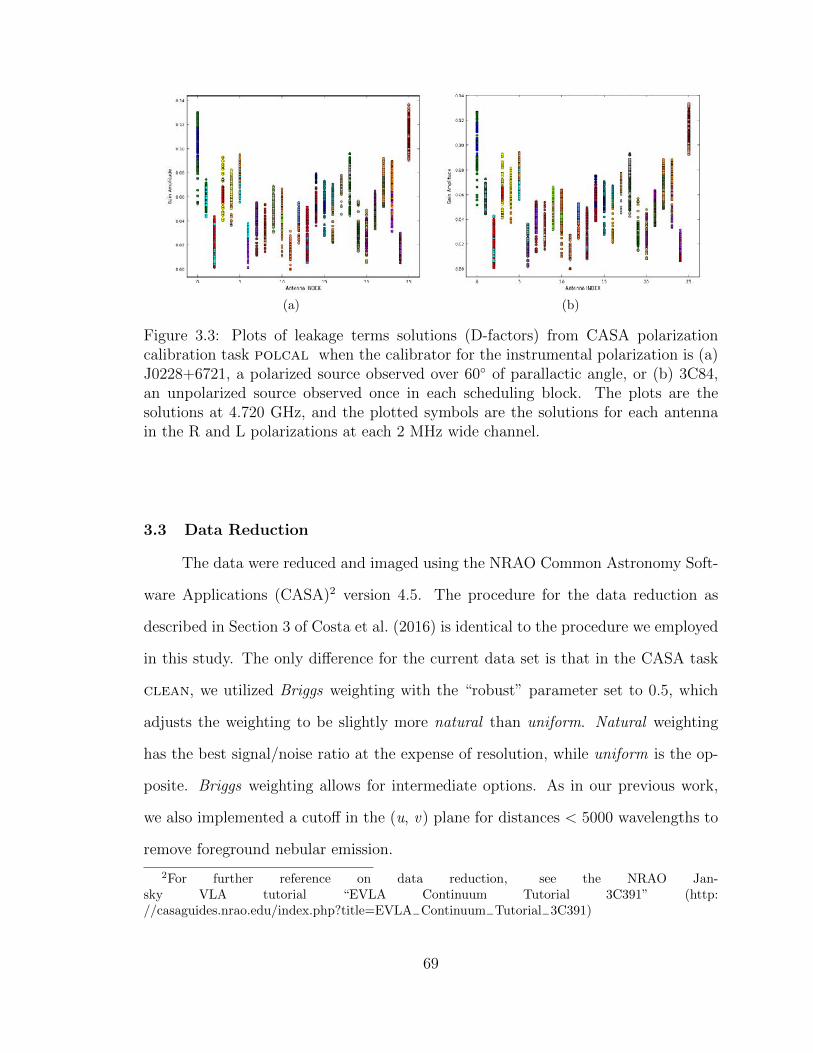
(a) (b)

Figure 3.3: Plots of leakage terms solutions (D-factors) from CASA polarizationcalibration task polcal when the calibrator for the instrumental polarization is (a)J0228+6721, a polarized source observed over 60 of parallactic angle, or (b) 3C84,an unpolarized source observed once in each scheduling block. The plots are thesolutions at 4.720 GHz, and the plotted symbols are the solutions for each antennain the R and L polarizations at each 2 MHz wide channel.

3.3 Data Reduction

The data were reduced and imaged using the NRAO Common Astronomy Soft-

ware Applications (CASA)2 version 4.5. The procedure for the data reduction as

described in Section 3 of Costa et al. (2016) is identical to the procedure we employed

in this study. The only difference for the current data set is that in the CASA task

clean, we utilized Briggs weighting with the “robust” parameter set to 0.5, which

adjusts the weighting to be slightly more natural than uniform. Natural weighting

has the best signal/noise ratio at the expense of resolution, while uniform is the op-

posite. Briggs weighting allows for intermediate options. As in our previous work,

we also implemented a cutoff in the (u, v) plane for distances < 5000 wavelengths to

remove foreground nebular emission.

2For further reference on data reduction, see the NRAO Jan-sky VLA tutorial “EVLA Continuum Tutorial 3C391” (http://casaguides.nrao.edu/index.php?title=EVLA−Continuum−Tutorial−3C391)

69

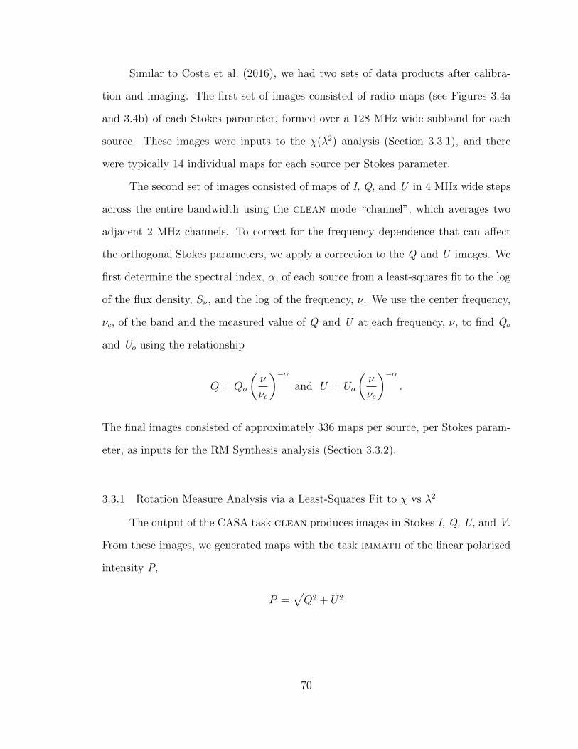
Similar to Costa et al. (2016), we had two sets of data products after calibra-

tion and imaging. The first set of images consisted of radio maps (see Figures 3.4a

and 3.4b) of each Stokes parameter, formed over a 128 MHz wide subband for each

source. These images were inputs to the χ(λ2) analysis (Section 3.3.1), and there

were typically 14 individual maps for each source per Stokes parameter.

The second set of images consisted of maps of I, Q, and U in 4 MHz wide steps

across the entire bandwidth using the clean mode “channel”, which averages two

adjacent 2 MHz channels. To correct for the frequency dependence that can affect

the orthogonal Stokes parameters, we apply a correction to the Q and U images. We

first determine the spectral index, α, of each source from a least-squares fit to the log

of the flux density, Sν , and the log of the frequency, ν. We use the center frequency,

νc, of the band and the measured value of Q and U at each frequency, ν, to find Qo

and Uo using the relationship

Q = Qo

(ν

νc

)−αand U = Uo

(ν

νc

)−α.

The final images consisted of approximately 336 maps per source, per Stokes param-

eter, as inputs for the RM Synthesis analysis (Section 3.3.2).

3.3.1 Rotation Measure Analysis via a Least-Squares Fit to χ vs λ2

The output of the CASA task clean produces images in Stokes I, Q, U, and V.

From these images, we generated maps with the task immath of the linear polarized

intensity P,

P =√Q2 + U2

70

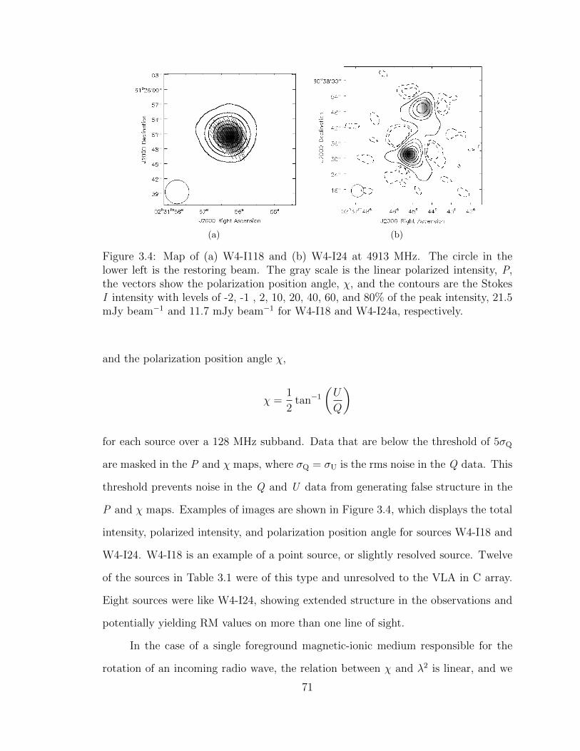
(a) (b)

Figure 3.4: Map of (a) W4-I118 and (b) W4-I24 at 4913 MHz. The circle in thelower left is the restoring beam. The gray scale is the linear polarized intensity, P,the vectors show the polarization position angle, χ, and the contours are the StokesI intensity with levels of -2, -1 , 2, 10, 20, 40, 60, and 80% of the peak intensity, 21.5mJy beam−1 and 11.7 mJy beam−1 for W4-I18 and W4-I24a, respectively.

and the polarization position angle χ,

χ =1

2tan−1

(U

Q

)

for each source over a 128 MHz subband. Data that are below the threshold of 5σQ

are masked in the P and χ maps, where σQ = σU is the rms noise in the Q data. This

threshold prevents noise in the Q and U data from generating false structure in the

P and χ maps. Examples of images are shown in Figure 3.4, which displays the total

intensity, polarized intensity, and polarization position angle for sources W4-I18 and

W4-I24. W4-I18 is an example of a point source, or slightly resolved source. Twelve

of the sources in Table 3.1 were of this type and unresolved to the VLA in C array.

Eight sources were like W4-I24, showing extended structure in the observations and

potentially yielding RM values on more than one line of sight.

In the case of a single foreground magnetic-ionic medium responsible for the

rotation of an incoming radio wave, the relation between χ and λ2 is linear, and we

71

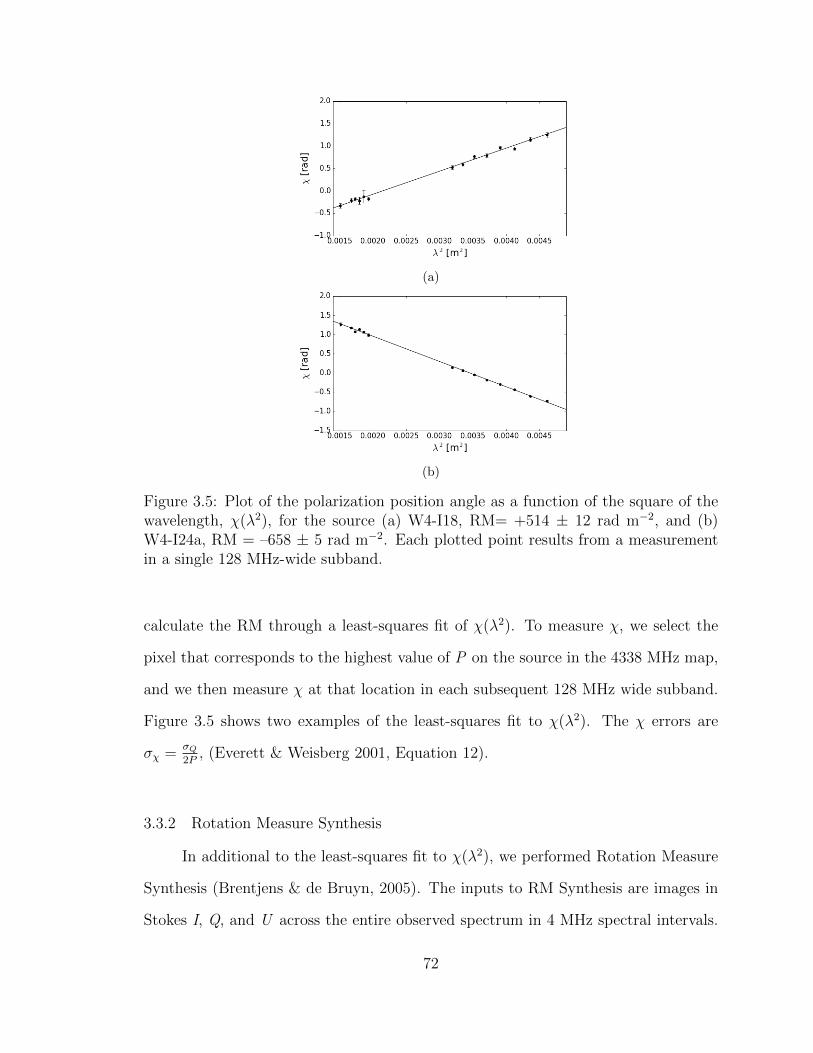
(a)

(b)

Figure 3.5: Plot of the polarization position angle as a function of the square of thewavelength, χ(λ2), for the source (a) W4-I18, RM= +514 ± 12 rad m−2, and (b)W4-I24a, RM = –658 ± 5 rad m−2. Each plotted point results from a measurementin a single 128 MHz-wide subband.

calculate the RM through a least-squares fit of χ(λ2). To measure χ, we select the

pixel that corresponds to the highest value of P on the source in the 4338 MHz map,

and we then measure χ at that location in each subsequent 128 MHz wide subband.

Figure 3.5 shows two examples of the least-squares fit to χ(λ2). The χ errors are

σχ =σQ2P, (Everett & Weisberg 2001, Equation 12).

3.3.2 Rotation Measure Synthesis

In additional to the least-squares fit to χ(λ2), we performed Rotation Measure

Synthesis (Brentjens & de Bruyn, 2005). The inputs to RM Synthesis are images in

Stokes I, Q, and U across the entire observed spectrum in 4 MHz spectral intervals.

72

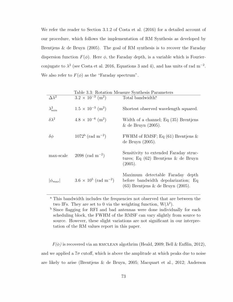
We refer the reader to Section 3.1.2 of Costa et al. (2016) for a detailed account of

our procedure, which follows the implementation of RM Synthesis as developed by

Brentjens & de Bruyn (2005). The goal of RM synthesis is to recover the Faraday

dispersion function F (φ). Here φ, the Faraday depth, is a variable which is Fourier-

conjugate to λ2 (see Costa et al. 2016, Equations 3 and 4), and has units of rad m−2.

We also refer to F (φ) as the “Faraday spectrum”.

Table 3.3: Rotation Measure Synthesis Parameters∆λ2 3.2 × 10−3 (m2) Total bandwidtha.

λ2min 1.5 × 10−3 (m2) Shortest observed wavelength squared.

δλ2 4.8 × 10−6 (m2) Width of a channel; Eq (35) Brentjens& de Bruyn (2005).

δφ 1072b (rad m−2) FWHM of RMSF; Eq (61) Brentjens &de Bruyn (2005).

max-scale 2098 (rad m−2)Sensitivity to extended Faraday struc-tures; Eq (62) Brentjens & de Bruyn(2005).

|φmax| 3.6 × 105 (rad m−2)Maximum detectable Faraday depthbefore bandwidth depolarization; Eq(63) Brentjens & de Bruyn (2005).

a This bandwidth includes the frequencies not observed that are between thetwo IFs. They are set to 0 via the weighting function, W(λ2).

b Since flagging for RFI and bad antennas were done individually for eachscheduling block, the FWHM of the RMSF can vary slightly from source tosource. However, these slight variations are not significant in our interpre-tation of the RM values report in this paper.

F(φ) is recovered via an rmclean algothrim (Heald, 2009; Bell & Enßlin, 2012),

and we applied a 7σ cutoff, which is above the amplitude at which peaks due to noise

are likely to arise (Brentjens & de Bruyn, 2005; Macquart et al., 2012; Anderson

73

et al., 2015). The rmsynthesis algorithm initially searched for peaks in the Faraday

spectrum using a range of φ ± 10,000 rad m−2 at a resolution of 40 rad m−2 to

determine if there were significant peaks at large values of |φ|. Then, we performed a

finer search at φ = ± 3000 rad m−2 at a resolution of 10 rad m−2. The RM Synthesis

parameters, such as the full-width-at-half-maximum (FWHM) of the rotation measure

spread function (RMSF) and the maximum detectable Faraday depth, are given in

Table 3.3.

(a)

(b)

Figure 3.6: (a) Linear polarization map and (b) RM map of W4-I24 from the RMSynthesis analysis. In both images, the data cube was flattened over the Faradaydepth axes, and a threshold of 7σ was applied. W4-I24 has extended structure, sothere are two peaks, which are also present in the CASA maps (Figure 3.4b).

74

As in Costa et al. (2016), we utilized an IDL code for the rmsynthesis and

rmclean algorithms. The output of the IDL code is a data cube in Faraday depth

space that is equal in range to the range of φ that was searched over in the rmsyn-

thesis algorithm. The data cube contains, for example, 500 maps of the polarized

intensity as a function of spatial coordinates and φ, which ranges between ± 10,000

rad m−2 at intervals of 40 rad m−2. Initially, we generated these maps for a 1024 ×

1024 pixel image. We then used the Karma package (Gooch, 1995) tool kvis to re-

view the maps to search for sources or source components away from the phase center

that, while being too weak to detect in the 128 MHz maps, may be detectable in the

RM Synthesis technique since it uses the entire bandwidth to determine the Faraday

spectrum3. However, no such sources were identified above the cutoff. From the 1024

× 1024 maps of the Faraday spectrum, we identified the Pmax for the observed sources

and extracted the Faraday spectrum at that location. Figure 3.6a shows an example

of a Pmax map that has been flattened along the φ axis, i.e., the gray scale in the

image represents the full range of φ. From this map, it is easy to identify the spatial

location of Pmax for the source, which agrees with the location of the peak linear

polarized intensity in the χ(λ2) analysis. We obtained this same result in Costa et al.

(2016) for the Rosette Nebula.

To determine the RM, we fit a 2 degree polynomial to the Faraday spectrum at

each pixel in the 1024 x 1024 image above the 7σ cutoff. The gray scale in Figure 3.6b

shows the RM value from the fit to each pixel. The image is zoomed and centered

on the source. While we can mathematically determine the RM at each pixel, the

sources are not resolved, so we only select the RM at the spatial location of Pmax.

Figure 3.7a plots the Faraday spectrum and rmclean components for W4-I18, and

Figure 3.7b shows the RMSF.

3private communication, L. Rudnick

75

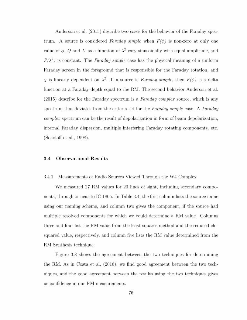
Anderson et al. (2015) describe two cases for the behavior of the Faraday spec-

trum. A source is considered Faraday simple when F(φ) is non-zero at only one

value of φ, Q and U as a function of λ2 vary sinusoidally with equal amplitude, and

P(λ2) is constant. The Faraday simple case has the physical meaning of a uniform

Faraday screen in the foreground that is responsible for the Faraday rotation, and

χ is linearly dependent on λ2. If a source is Faraday simple, then F(φ) is a delta

function at a Faraday depth equal to the RM. The second behavior Anderson et al.

(2015) describe for the Faraday spectrum is a Faraday complex source, which is any

spectrum that deviates from the criteria set for the Faraday simple case. A Faraday

complex spectrum can be the result of depolarization in form of beam depolarization,

internal Faraday dispersion, multiple interfering Faraday rotating components, etc.

(Sokoloff et al., 1998).

3.4 Observational Results

3.4.1 Measurements of Radio Sources Viewed Through the W4 Complex

We measured 27 RM values for 20 lines of sight, including secondary compo-

nents, through or near to IC 1805. In Table 3.4, the first column lists the source name

using our naming scheme, and column two gives the component, if the source had

multiple resolved components for which we could determine a RM value. Columns

three and four list the RM value from the least-squares method and the reduced chi-

squared value, respectively, and column five lists the RM value determined from the

RM Synthesis technique.

Figure 3.8 shows the agreement between the two techniques for determining

the RM. As in Costa et al. (2016), we find good agreement between the two tech-

niques, and the good agreement between the results using the two techniques gives

us confidence in our RM measurements.

76

Table 3.4: Faraday Rotation Measurement Values through the W4 Complex

Source ComponentRMa Reduced RMc ξd ξe

(rad m−2) χ2b (rad m−2) (pc) (pc)W4-I1 a -277 ± 1 29 -258 ± 3 29 53

W4-I2a -1042 ± 7 1.5 -930 ± 30

30 26b -935 ± 6 1.5 -954 ± 11

W4-I3 a -876 ± 2 1.9 -878 ± 8 27 16

W4-I4a -139 ± 3 1.9 -153 ± 12

38 59b -91 ± 6 2 -68 ± 15

W4-I6 a -990 ± 8 1.3 -961 ± 23 29 25W4-I8 a -276 ± 2 4.4 -337 ± 8 37 54W4-I11 a -377 ± 8 12 -141 ± 18 35 41W4-I12 a -315 ± 4 2.8 -306 ± 10 34 54

W4-I13a -777 ± 8 1.2 -801 ± 24

28 36b -701 ± 28 0.5 -772 ± 66

W4-I14 a -678 ± 27 0.6 -666 ± 66 20 36W4-I15 a -157 ± 9 0.8 -124 ± 14 32 10

W4-I17a -492 ± 8 1.6 -440 ± 40

11 31b -509 ± 15 0.6 -464 ± 40

W4-I18 a +514 ± 12 1.1 +501 ± 33 4 22W4-I19 a -407 ± 14 0.3 -431 ± 36 37 34

W4-I21a -53 ± 26 1.4 -167 ± 67

17 15b -98 ± 28 0.5 -79 ± 62c -173 ± 34 0.5 -232 ± 70

W4-I24a -658 ± 5 1.4 -678 ± 14

39 23b -675 ± 12 0.4 -716 ± 30

W4-O4 a -31 ± 12 24 -178 ± 18 68 81W4-O6 a -95 ± 1 3.6 -96 ± 4 54 76W4-O7 a -175 ± 24 0.8 -256 ± 56 53 62W4-O10 a -379 ± 5 1.8 -343 ± 16 56 66a RM value obtained from a least-squares linear fit to χ(λ2). The errors

are 1σ.b Reduced χ2 for the χ(λ2) fit.c Effective RM derived from RM Synthesis.d Distance from center of OCl 352.e Distance from Terebey et al. (2003) center.

77

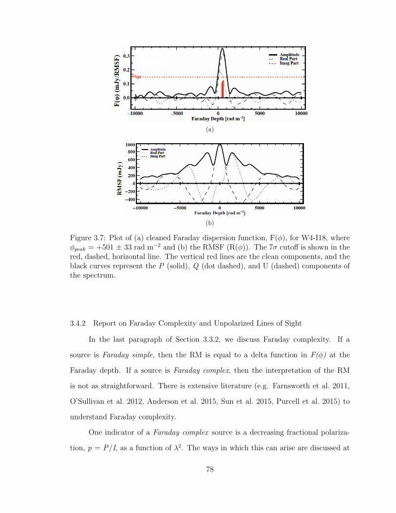
(a)

(b)

Figure 3.7: Plot of (a) cleaned Faraday dispersion function, F(φ), for W4-I18, whereφpeak = +501 ± 33 rad m−2 and (b) the RMSF (R(φ)). The 7σ cutoff is shown in thered, dashed, horizontal line. The vertical red lines are the clean components, and theblack curves represent the P (solid), Q (dot dashed), and U (dashed) components ofthe spectrum.

3.4.2 Report on Faraday Complexity and Unpolarized Lines of Sight

In the last paragraph of Section 3.3.2, we discuss Faraday complexity. If a

source is Faraday simple, then the RM is equal to a delta function in F(φ) at the

Faraday depth. If a source is Faraday complex, then the interpretation of the RM

is not as straightforward. There is extensive literature (e.g. Farnsworth et al. 2011,

O’Sullivan et al. 2012, Anderson et al. 2015, Sun et al. 2015, Purcell et al. 2015) to

understand Faraday complexity.

One indicator of a Faraday complex source is a decreasing fractional polariza-

tion, p = P/I, as a function of λ2. The ways in which this can arise are discussed at

78

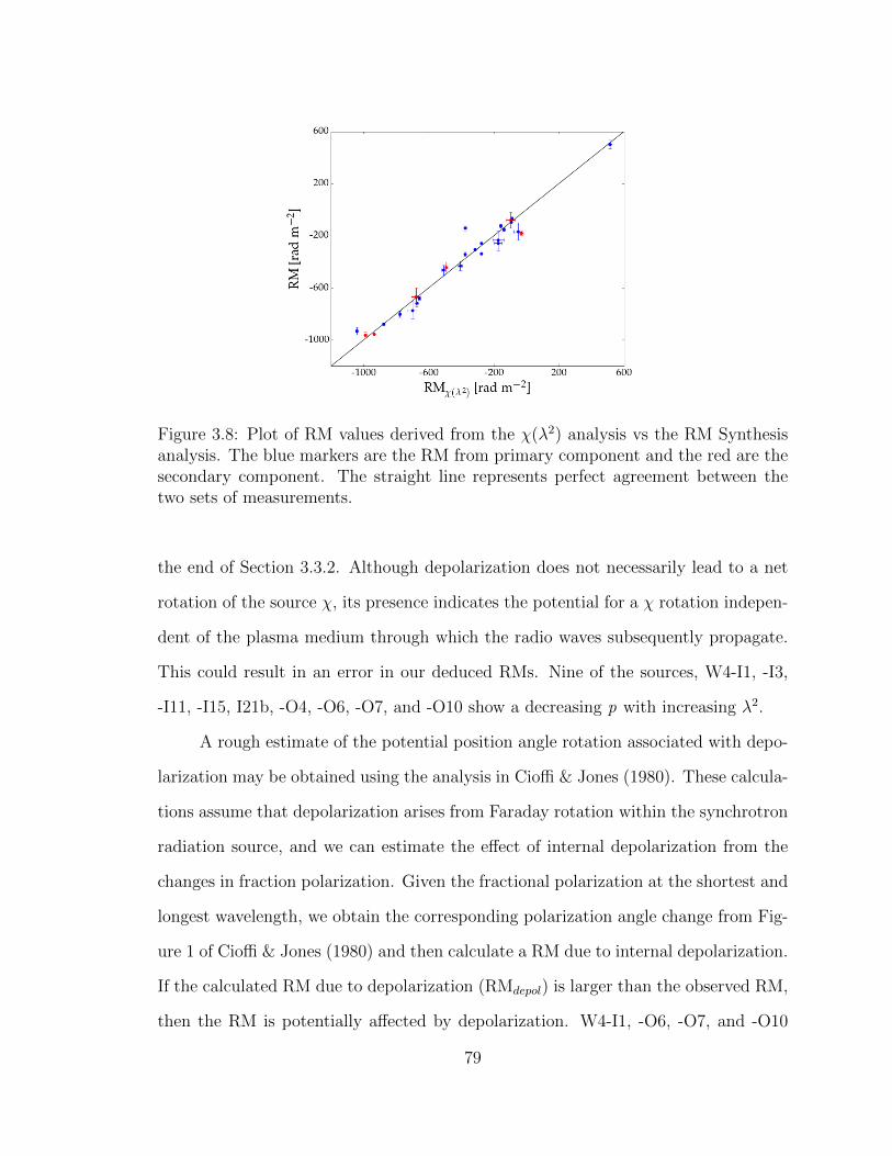
Figure 3.8: Plot of RM values derived from the χ(λ2) analysis vs the RM Synthesisanalysis. The blue markers are the RM from primary component and the red are thesecondary component. The straight line represents perfect agreement between thetwo sets of measurements.

the end of Section 3.3.2. Although depolarization does not necessarily lead to a net

rotation of the source χ, its presence indicates the potential for a χ rotation indepen-

dent of the plasma medium through which the radio waves subsequently propagate.

This could result in an error in our deduced RMs. Nine of the sources, W4-I1, -I3,

-I11, -I15, I21b, -O4, -O6, -O7, and -O10 show a decreasing p with increasing λ2.

A rough estimate of the potential position angle rotation associated with depo-

larization may be obtained using the analysis in Cioffi & Jones (1980). These calcula-

tions assume that depolarization arises from Faraday rotation within the synchrotron

radiation source, and we can estimate the effect of internal depolarization from the

changes in fraction polarization. Given the fractional polarization at the shortest and

longest wavelength, we obtain the corresponding polarization angle change from Fig-

ure 1 of Cioffi & Jones (1980) and then calculate a RM due to internal depolarization.

If the calculated RM due to depolarization (RMdepol) is larger than the observed RM,

then the RM is potentially affected by depolarization. W4-I1, -O6, -O7, and -O10

79

show RMdepol ∼ RMobs, which indicates that internal depolarization could affect the

observed RM. The observed RM of W4-I3 is ∼ 3 times larger than RMdepol, so it is

not affected by internal depolarization.

Depolarization due to internal Faraday rotation makes predictions for the form

of χ(λ2) which would not have χ ∝ λ2 (Cioffi & Jones, 1980). For all of the sources

mentioned above, we compared the observed behavior of χ(λ2) to the predicted be-

havior (Equation 4b of Cioffi & Jones 1980). Within the errors, only W4-O7 is

consistent with the non-linear behavior of a RM affected by internal depolarization.

We interpret this result as meaning that our deduced RM values for most of the

sources are not significantly in error due to internal depolarization, and we consider

the measurement of depolarization as providing a cautionary flag.

We also considered whether our measurements could have been affected by

bandwidth depolarization or beam depolarization. Bandwidth depolarization occurs

when the polarization angle varies over frequency averaged bins, ∆ν. For example

in this study, we use values of χ in 128 MHz wide bins (Section 3.3.1) and 4 MHz

(Section 3.3.2). For a center frequency of the lowest frequency bin, we use νc = 4466

MHz, and the relationship between the change in polarization position angle, ∆χ, is

|∆χ| = 2|RM| c2 ∆ν

ν3c

, (3.3)

where c is the speed of light. This formula shows that even for |RM| = 104 rad m−2,

which is far larger than any RMs we measure, the Faraday rotation across the band

is 0.41 radians. This is insufficient to causes substantial bandwidth depolarization.

Beam depolarization occurs when there are small scale variations of the electron

density or the magnetic field within a beam. It is unlikely that the RMs are affected

by beam depolarization as the beam at 6 cm for the VLA in C array is ∼ 5 arcseconds.

We interpret these RMs as a characteristic value due to the plasma medium (primarily

80

the Galactic ISM) between the source and the observer. In the analysis which follows,

we choose the RM values from the RM Synthesis method.

When the data were mapped and inspected, we found that a few sources that

had passed our criteria for flux density and compactness to the VLA D array at L band

(1.42 GHz) were completely unpolarized. W4-I16 and W4-O8 are not polarized at any

frequency, and the RM Synthesis technique does not show significant (> 7σ) peaks at

any φ. Three of the lines of sight, W4-I5, W4-I10, and W4-I22, have no source in the

field. Despite appearing to be point sources in the NVSS postage stamps (see Section

3.2), we do not observe a source at these locations, and they may have been clumpy

foreground nebular emission that was filtered out during the imaging process.

Subsequent investigations determined that some of the selected sources were

previously cataloged ultra compact H ii regions associated with the W3 star forma-

tion region. These sources are W4-I7 (W3(OH)-C), W4-I9 (AFGL 333), and W4-I20

(W3(OH)-A) (Feigelson & Townsley, 2008; Navarete et al., 2011; Roman-Zuniga et al.,

2015). The W4-I7 field has no source at the observed α and δ, despite it being identi-

fied as W3(OH)-C. We do not observe a source at this location in any frequency bin.

W3(OH)-A, however, is observed and is a point source in our maps at all frequencies.

Similarly, W4-I9 is detected in each frequency bin and is an extended source. These

sources are unpolarized and do not feature in our subsequent analysis.

3.4.3 A Unique Line of Sight Through the W4 Region: LSI +61303

W4-I19 has a spectrum which is inconsistent with an optically-thin extragalactic

radio source. It is linearly polarized, and we measure RM = –431 ± 36 rad m−2.

Investigation of this source during the data analysis phase revealed that it is not an

extragalactic source, although it passed our selection criteria for flux and compactness.

W4-I19 is the high mass X-ray binary (HMXB) LSI +61303 (Gregory et al., 1979;

Bignami et al., 1981), which is notable for being one of five known gamma ray binary

81

systems (Frail & Hjellming, 1991). This system has been extensively studied, and

as a result, much is known about the nature of the compact object (Massi et al.,

2004; Massi, 2004; Dubus, 2006; Paredes et al., 2007; Massi et al., 2017), the stellar

companion (Casares et al., 2005; Dubus, 2006; Paredes et al., 2007), orbital period

(Gregory & Neish, 2002), radio structure (Albert et al., 2008), and radial velocity

(Gregory et al., 1979; Lestrade et al., 1999).

The spatial location of LSI +61303 is important to understanding the RM we

determined for this source. Frail & Hjellming (1991) argue that since signatures of the

Perseus arm shock are present in the absorption spectrum to LSI +61303 but not the

post-shock gas from the Perseus arm, LSI +61303 must lie between the two features

at a distance of 2.0 ± 0.2 kpc. They also report that they do not see absorption

features due to the IC 1805 ionization front and shock front. The estimated distance

to LSI +61303 is consistent with distance estimates to OCl 352. The position relative

to the nebula has consequences for the interpretation of the RM that we measure.

The possibilities are:

1. LSI +61303 is in front of the stellar bubble and H ii region, so it is exterior to

a region modified by OCl 352. The RM is then an estimate of the foreground

ISM between us and the nebula.

2. If LSI +61303 is at the same distance as IC 1805 or slightly behind (greater

distance), then the RM is unique among our sources in that it is not affected by

Faraday rotation from material in the outer Galaxy. The RM is then probing

at least a part of the Faraday rotating material due to the nebula.

To further determine the position of LSI +61303 with respect to IC 1805, we

review the current state of knowledge on the subject from the literature. Dhawan et al.

(2006) observed LSI +61303 with the Very Long Baseline Array (VLBA) and report

a proper motion of (µα, µδ) = (-0.30 ± 0.07, -0.26 ± 0.05) mas yr−1. Aragona et al.

82

(2009) report a radial velocity for LSI +61303 of Vrad = –41.4 ± 0.6 km s−1, which

agrees with previous estimates by Casares et al. (2005). For OCl 352, Dambis et al.

(2001) estimate the radial velocity to be –41 ± 3 km s−1, and more recent estimates by

Kharchenko et al. (2005) (Vrad = –47 ± 18 km s−1) agree within the errors. Both LSI

+61303 and OCl 352 have similar radial velocities, and the proper motion estimates

by Dhawan et al. (2006) indicate that LSI +61303 is moving similarly on the plane

of the sky to OCl 352, which has a proper motion of (µα, µδ) = (–1.0 ± 0.4, –0.9 ±

0.4) mas yr−1 (Dambis et al., 2001).

From proper motion and radial velocity estimates, LSI +61303 appears to be

moving in relatively the same direction and speed as OCl 352. Using a distance of 2

kpc to LSI +61303 and 2.2 kpc to OCl 352, the transverse velocities are ∼ 3 km s−1

and ∼ 14 km s−1, respectively. If LSI +61303 originally belonged to OCl 352, then

it is unlikely that it is in front of IC 1805, given that both are moving at the same

radial velocity. While LSI +61303 appears to be outside the obvious shell structure

of IC 1805, it is more likely that it is probing material modified by OCl 352. We

discuss this possibility further in Section 3.5.3.

If LSI +61303 did not originate in OCl 352, then it is possible to still be in

front of the nebula, despite the similar velocities. In such a case, the RM we obtained

for this line of sight is due to the ISM between us and IC 1805. The RM value we find

for LSI +61303 is nearly 3 times larger than the background RM, which we discuss

in Section 3.5.2. This would require a magneto-ionic medium between the observer

and the nebula capable of producing ∼ 400 rad m−2 along this line of sight. As may

be seen from Table 3.4 and Figure 3.2, other lines of sight near IC 1805, but exterior

to the shell, do not have as large of RM values (e.g. W4-O26, -O19, -O7, -I11). It

therefore seems most probable that the RM for W-I19 (LSI +61303) is dominated

by plasma in W4.

In summary, there is evidence in the literature that suggests LSI +61303 may

83

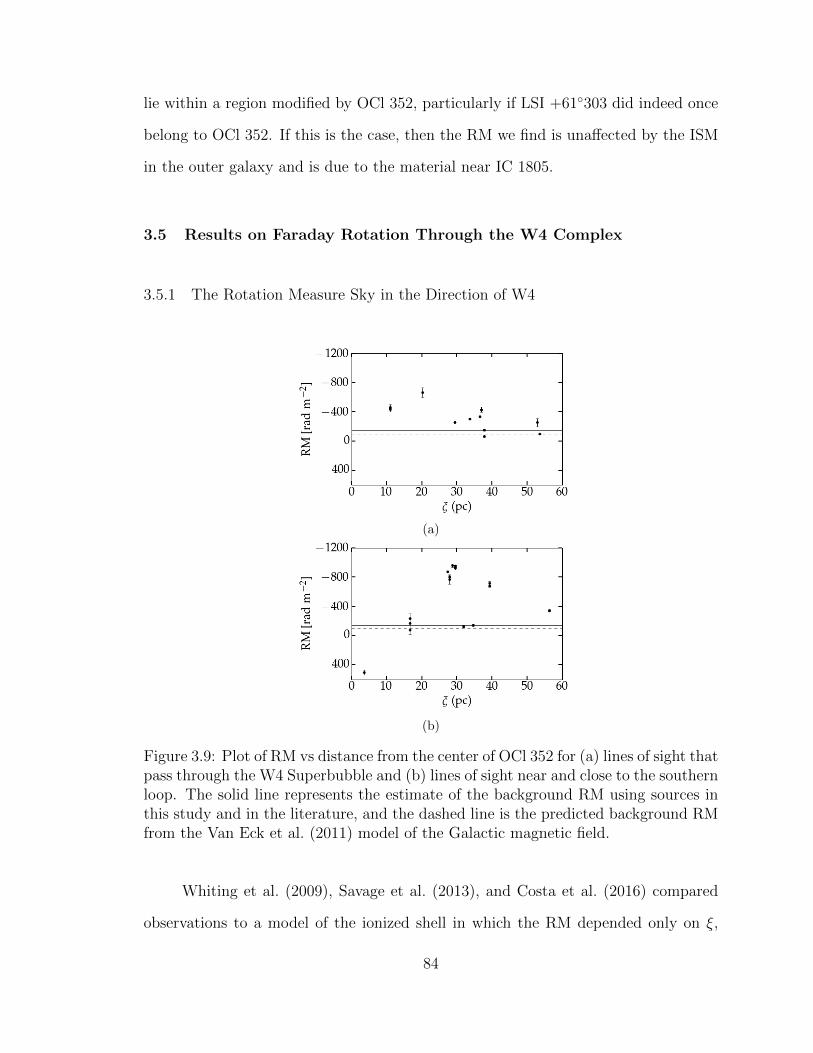
lie within a region modified by OCl 352, particularly if LSI +61303 did indeed once

belong to OCl 352. If this is the case, then the RM we find is unaffected by the ISM

in the outer galaxy and is due to the material near IC 1805.

3.5 Results on Faraday Rotation Through the W4 Complex

3.5.1 The Rotation Measure Sky in the Direction of W4

(a)

(b)

Figure 3.9: Plot of RM vs distance from the center of OCl 352 for (a) lines of sight thatpass through the W4 Superbubble and (b) lines of sight near and close to the southernloop. The solid line represents the estimate of the background RM using sources inthis study and in the literature, and the dashed line is the predicted background RMfrom the Van Eck et al. (2011) model of the Galactic magnetic field.

Whiting et al. (2009), Savage et al. (2013), and Costa et al. (2016) compared

observations to a model of the ionized shell in which the RM depended only on ξ,

84

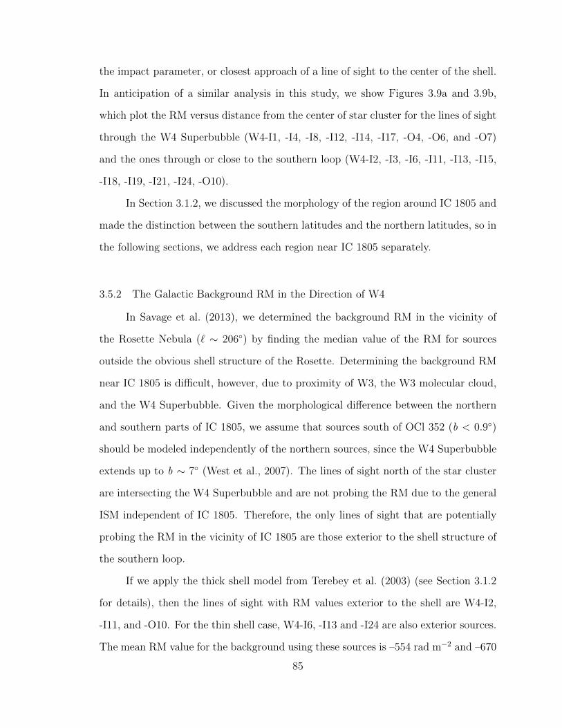
the impact parameter, or closest approach of a line of sight to the center of the shell.

In anticipation of a similar analysis in this study, we show Figures 3.9a and 3.9b,

which plot the RM versus distance from the center of star cluster for the lines of sight

through the W4 Superbubble (W4-I1, -I4, -I8, -I12, -I14, -I17, -O4, -O6, and -O7)

and the ones through or close to the southern loop (W4-I2, -I3, -I6, -I11, -I13, -I15,

-I18, -I19, -I21, -I24, -O10).

In Section 3.1.2, we discussed the morphology of the region around IC 1805 and

made the distinction between the southern latitudes and the northern latitudes, so in

the following sections, we address each region near IC 1805 separately.

3.5.2 The Galactic Background RM in the Direction of W4

In Savage et al. (2013), we determined the background RM in the vicinity of

the Rosette Nebula (` ∼ 206) by finding the median value of the RM for sources

outside the obvious shell structure of the Rosette. Determining the background RM

near IC 1805 is difficult, however, due to proximity of W3, the W3 molecular cloud,

and the W4 Superbubble. Given the morphological difference between the northern

and southern parts of IC 1805, we assume that sources south of OCl 352 (b < 0.9)

should be modeled independently of the northern sources, since the W4 Superbubble

extends up to b ∼ 7 (West et al., 2007). The lines of sight north of the star cluster

are intersecting the W4 Superbubble and are not probing the RM due to the general

ISM independent of IC 1805. Therefore, the only lines of sight that are potentially

probing the RM in the vicinity of IC 1805 are those exterior to the shell structure of

the southern loop.

If we apply the thick shell model from Terebey et al. (2003) (see Section 3.1.2

for details), then the lines of sight with RM values exterior to the shell are W4-I2,

-I11, and -O10. For the thin shell case, W4-I6, -I13 and -I24 are also exterior sources.

The mean RM value for the background using these sources is –554 rad m−2 and –670

85

Table 3.5: List of Sources with RM values from CatalogsSource α(J2000) δ(J2000) RMa

Name h m s o ′ ′′ (rad m2)W4-O3 02 35 43.0 +63 22 33.0 –138b± 18W4-O19 02 46 23.9 +61 33 19.9 –157c± 15W4-O26 02 42 32.3 +60 02 31.0 +61 ± 41W4-O27 02 25 48.7 +59 53 52.0 –145 ± 22a RM values from Brown et al. (2003) unless oth-

erwise noted.b Taylor et al. (2009) give –75 ± 9 rad m−2 for

this line of sight.c RM value from Taylor et al. (2009).

rad m−2 for the thick or thin shell, respectively. In Table 3.5, we list RM values from

the literature for lines of sight near IC 1805 that we include in our estimate of the

background RM. The mean RM value for these sources (excluding W4-O3 for being in

the superbubble) is –80 rad m−2. The sources W4-I2, -I6, -I13, and -I24 are seemingly

outside the obvious ionized shell structure; however, they are also the lines of sight

for which we measure some of the highest RM values. This is a surprising result, and

one we did not observe in the case of the Rosette Nebula. It strongly suggests that

the lines of sight to W4-I2, -I6, -I13, and -I24 have RMs that are dominated by the

W4 complex, despite the fact that they are outside the obvious ionized shell of IC

1805. We discuss this further in the next section.

For the present discussion, we exclude these sources from the estimate of the

background. Using W4-I11, -O10, -O19, -O26, and -O27, we find a mean value for

the background RM due to the ISM of –145 rad m−2. While this value is similar in

magnitude to the value of the background RM we found in our studies on the Rosette

Nebula, we have significantly fewer lines of sight, and only two of the lines of sight

were observed in this study.

Due to a low number of lines of sight exterior to IC 1805, we utilize the model

of a Galactic magnetic field by Van Eck et al. (2011) to estimate the background RM

86

due to the ISM. From their Figure 6, they find the Galactic magnetic field is best

modeled by an almost purely azimuthal, clockwise field. Van Eck et al. (2011) use

their model to predict the RM values in the Galaxy, and in the vicinity of IC 1805,

their model predicts RMs of order –100 rad m−2. Using this as an estimate of the

background RM, we find an excess RM due to IC 1805 of +600 to –860 rad m−2.

3.5.3 High Faraday Rotation Through Photodissociation Regions

The lines of sight with the highest RM values, W4-I2, -I6, and -I24, appear to

be outside the obvious shell of the southern loop. These sources are very near to

the bright ionized shell. Terebey et al. (2003) and Gray et al. (1999) discuss a halo

of ionized gas that surrounds IC 1805, which may be causing the high RM values.

Gray et al. (1999) speculate that the diffuse extended structure is an extended H ii

envelope as suggested by Anantharamaiah (1985). Another possibility is that these

high RMs arise in the PDR surrounding the IC 1805 H ii region.

PDRs are the regions between ionized gas, which is fully ionized by photons

with hν > 13.6 eV, and neutral or molecular material. PDRs can be partially ionized

and heated by far-ultraviolet photons (6 eV < hν < 13.6 eV) (Tielens & Hollenbach,

1985; Hollenbach & Tielens, 1999). Typically, the PDR consists of neutral hydrogen,

ionized carbon, and neutral oxygen nearest to the ionization front, and with increasing

distance, molecular species (e.g., CO, H2, and O2) dominate the chemical composition

of a PDR (Hollenbach & Tielens, 1999). One tracer of PDRs is polycyclic aromatic

hydrocarbon (PAH) emission at infrared (IR) wavelengths. Churchwell et al. (2006)

identify more than 300 bubbles at IR wavelengths in the Galactic Legacy Infrared

Mid-Plane Survey Extraordinaire (GLIMPSE), and 25% of these bubble coincide with

known H ii regions. Watson et al. (2008) examine three bubbles from the Churchwell

et al. (2006) catalog with the Spitzer Infrared Array Camera (IRAC) bands 4.5, 5.8,

and 8.0 µm and the 24 µm band from the Spitzer Multiband Imaging Photometer

87

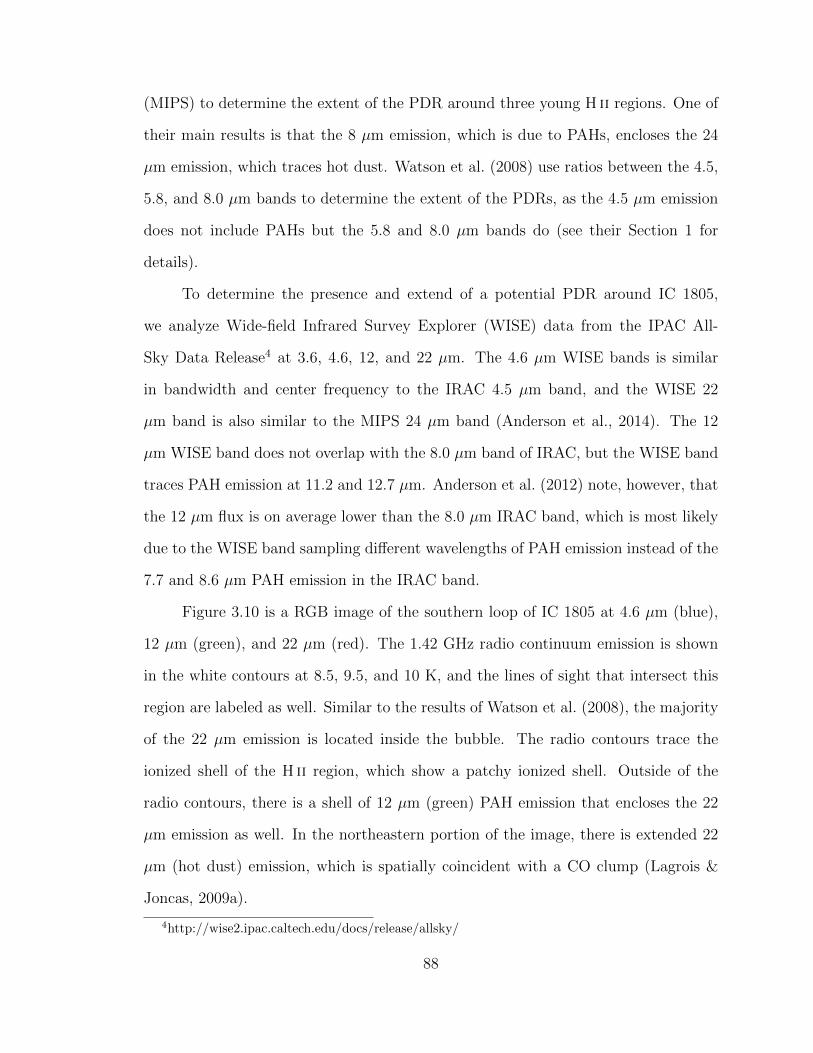
(MIPS) to determine the extent of the PDR around three young H ii regions. One of

their main results is that the 8 µm emission, which is due to PAHs, encloses the 24

µm emission, which traces hot dust. Watson et al. (2008) use ratios between the 4.5,

5.8, and 8.0 µm bands to determine the extent of the PDRs, as the 4.5 µm emission

does not include PAHs but the 5.8 and 8.0 µm bands do (see their Section 1 for

details).

To determine the presence and extend of a potential PDR around IC 1805,

we analyze Wide-field Infrared Survey Explorer (WISE) data from the IPAC All-

Sky Data Release4 at 3.6, 4.6, 12, and 22 µm. The 4.6 µm WISE bands is similar

in bandwidth and center frequency to the IRAC 4.5 µm band, and the WISE 22

µm band is also similar to the MIPS 24 µm band (Anderson et al., 2014). The 12

µm WISE band does not overlap with the 8.0 µm band of IRAC, but the WISE band

traces PAH emission at 11.2 and 12.7 µm. Anderson et al. (2012) note, however, that

the 12 µm flux is on average lower than the 8.0 µm IRAC band, which is most likely

due to the WISE band sampling different wavelengths of PAH emission instead of the

7.7 and 8.6 µm PAH emission in the IRAC band.

Figure 3.10 is a RGB image of the southern loop of IC 1805 at 4.6 µm (blue),

12 µm (green), and 22 µm (red). The 1.42 GHz radio continuum emission is shown

in the white contours at 8.5, 9.5, and 10 K, and the lines of sight that intersect this

region are labeled as well. Similar to the results of Watson et al. (2008), the majority

of the 22 µm emission is located inside the bubble. The radio contours trace the

ionized shell of the H ii region, which show a patchy ionized shell. Outside of the

radio contours, there is a shell of 12 µm (green) PAH emission that encloses the 22

µm emission as well. In the northeastern portion of the image, there is extended 22

µm (hot dust) emission, which is spatially coincident with a CO clump (Lagrois &

Joncas, 2009a).

4http://wise2.ipac.caltech.edu/docs/release/allsky/

88

The PDR model predicts the presence of neutral hydrogen and molecular CO

(see Figure 3 of Hollenbach & Tielens 1999) at increasing distance from the exciting

star cluster. Figure 1 of Sato (1990) and Figure 2 of Hasegawa et al. (1983) show

H i contours in the vicinity of IC 1805, and the H i emission appears to completely

enclose the southern loop except near 135.5 ≤ ` ≤ 136, 0.2≤ b ≤ 0.9. Braunsfurth

(1983) report H i emission near IC 1805, and he notes that the hole could be due to

cold H i gas or the lack of gas if the winds have sufficiently swept the material away

or ionized it. Figure 6 of Digel et al. (1996) shows the CO emission, with the W3

molecular cloud on the western side of IC 1805, CO emission along the southern loop

of IC 1805, and the molecular material associated with the W5 (` = 137.1, b = +0.89)

H ii region on the eastern side of IC 1805. We interpret the WISE data, the radio

contours, and the CO and H i maps as a patchy ionized shell surrounded by a PDR.

If there is a PDR surrounding IC 1805, then the highest RM values from our

data set, RM = –954 rad m−2 and –961 rad m−2 for W4-I2 and -I6, respectively, lie

outside the ionized shell of the H ii region and in the PDR. Similarly, the sources W4-

I19 and -I24 are also outside the radio continuum contours but appear to be within

the 12 µm (green) emission. This is a surprising result compared with our results

from the Rosette Nebula, where we found the highest RM values for lines of sight

that pass through the ionized shell. Gray et al. (1999) note zones of depolarization

near the southern portion of IC 1805, which require RMs on order 103 rad m−2, and

spatial RM gradients. The RMs for W4-I2 and -I6 are on this order, but those for

W4-I24 and -I19 are not, and we do not find that these lines of sight are affect by

depolarization. W4-I24 has two components for which we measure RMs, and the

components are separated by ∼ 18 arcseconds. The ∆RM, which is the difference in

RM between the two components is 38 rad m−2, which is not a large change in the

RM and is consistent within the errors.

The presence of the PDR is complicated, however, by the extended diffusion

89

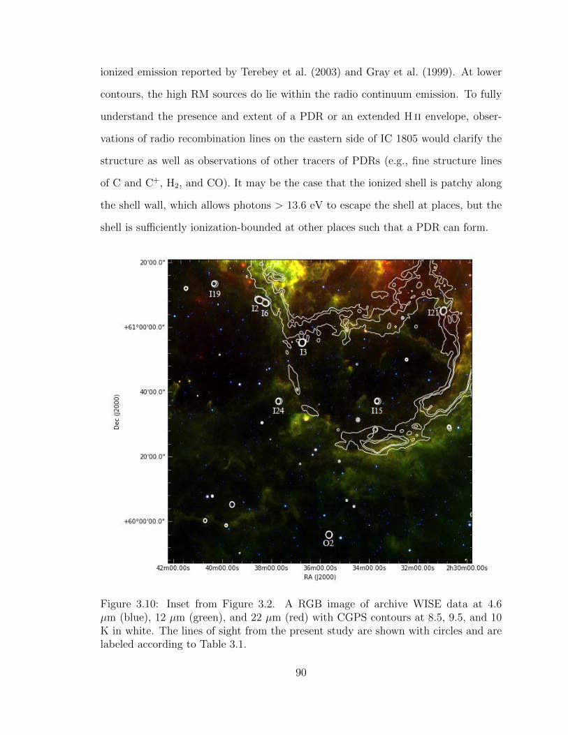
ionized emission reported by Terebey et al. (2003) and Gray et al. (1999). At lower

contours, the high RM sources do lie within the radio continuum emission. To fully

understand the presence and extent of a PDR or an extended H ii envelope, obser-

vations of radio recombination lines on the eastern side of IC 1805 would clarify the

structure as well as observations of other tracers of PDRs (e.g., fine structure lines

of C and C+, H2, and CO). It may be the case that the ionized shell is patchy along

the shell wall, which allows photons > 13.6 eV to escape the shell at places, but the

shell is sufficiently ionization-bounded at other places such that a PDR can form.

Figure 3.10: Inset from Figure 3.2. A RGB image of archive WISE data at 4.6µm (blue), 12 µm (green), and 22 µm (red) with CGPS contours at 8.5, 9.5, and 10K in white. The lines of sight from the present study are shown with circles and arelabeled according to Table 3.1.

90

3.5.4 Faraday Rotation Through the Cavity and Shell of the Stellar Bubble

There are four lines of sight are through the cavity of the stellar bubble, assum-

ing an inner radius from the Terebey et al. (2003) model. The sources W4-I3, -I15,

-I18, and -I21 are through the cavity, and including multiple components, we find 6

RM values. W4-I3 has a high RM (–878 ± 18 rad m−2), and W4-I15 and -I21 have

comparatively low RM values ( –79 to –232 rad m−2). Examination of Figures 3.2

and 3.10 does not reveal enhanced emission near W4-I3 in comparison to W4-I21.

W4-I15, however, is in a region of relatively low emission, which may explain why

W4-I15 has a RM value at least 4 times smaller than W4-I3.

W4-I13 is outside the shell, assuming a shell radius from either Terebey et al.

(2003) model. From Figure 3.2, it does appear to be outside the ionized shell. However

W4-I13 is within a 8.5 K contour on the 1.42 GHz radio continuum map, which may

indicate that it is probing the ionized shell. We find a high RM for both components

of this source, which is similar to the RM values for W4-I2 and -I6.

Across IC 1805, we observe negative RM values for all lines of sight except one:

W4-I18, which is 5.6 arcmin (4 pc) from the center of the star cluster. The absolute

value of the RM for W4-I18 is also large (+501 ± 33 rad m−2), indicating a large

change in RM along this line of sight relative to other lines of sight in this part of

the sky. This line of sight is probing the space close to the massive O and B stars

responsible for IC 1805. In the Weaver et al. (1977) model for a stellar bubble, the

hypersonic stellar wind dominates the region between the star responsible for the

bubble and the inner termination shock. Equation (12) of Weaver et al. (1977) states

that the distance of the inner shock, Rt is

Rt = 0.90 α3/2

(1

ρ0

dMw

dt

)3/10

V 1/10w t2/5, (3.4)

91

where α is a constant equal to 0.88, ρ0 is the mass density in the external ISM,

dMw/dt is the mass loss rate, Vw is the terminal wind speed, and t is time. For a

rough estimate of the inner shock distance, we utilize general stellar parameters for

OCl 352 of dMw/dt = 10−5 M yr−1, t = 106 yr, and Vw = 2200 km s−1(see Section

3.1.2 or Table 3.7). From the discussion in Section 3.6.2, we adopt n0 = 4.5 cm−3 for

ρ0 = n0mp, where mp is the mass of a proton. With these values in the appropriate

SI units, Rt ∼ 6 pc. It is possible that the line of sight to W4-I18 passes inside the

inner shock, and the large, positive RM is due to material modified by the hypersonic

stellar wind and not the shocked interstellar material. With a positive value of the

RM for W4-I18, the line of sight component of the field points towards us while the

remaining lines of sight in the cavity are negative, meaning BLOS points away.

3.5.5 Low Rotation Measure Values Through the W4 Superbubble

North of IC 1805 is the W4 Superbubble, which is an extended “egg-shaped”

structure closed at b ∼ 7 (West et al., 2007). Basu et al. (1999) utilize an Hα map to

define the shape, which would include the southern loop (134< ` < 136, b < 0.5);

Normandeau et al. (1996) examine the H i distribution, however, and place the base

of the structure at OCl 352. Similarly, West et al. (2007) place an offset bottom of

the “egg” at OCl 352. The southern loop of IC 1805 is seemingly sufficiently different

from the northern latitudes, as it is often not included in the discussion of the W4

Superbubble in spite of the fact that OCl 352 is thought to be responsible for the

formation of both structures (Terebey et al., 2003; West et al., 2007).

Nine lines of sight in the present study are north of OCl 352 in the W4 Super-

bubble. These sources are W4-I1, -I4, -I8, -I12, -I14, -I17, -O4, -O6, and -O7, and

they have a mean RM of –293 rad m−2 and a standard deviation of 178 rad m−2. Of

these sources, W4-I14 and -I17 have the largest RM values, –666 rad m−2 and –460

rad m−2, respectively, and they are close to OCl 352, with distances of 31 arcminutes

92

(20 pc) and 17 arcminutes (11 pc), respectively. As discussed in Section 3.1.2, Lagrois

& Joncas (2009a) argue that the ionized “v” structure north of OCl 352 is part of the

bubble wall and not a cap to southern loop structure, but examination of Figure 3.2

suggests that the bubble walls are denser, or thicker, at latitudes < 1.5 than higher

latitudes, which may explain the larger RM associated with W4-I14 and -I17. The

remaining lines of sight, however, in the W4 Superbubble have some of the lowest RM

values in the data set and are consistently lower RM values than the lines of sight

through the PDR.

At higher latitudes, Gao et al. (2015) modeled the polarized emission and ap-

plied a Faraday screen model to the W4 Superbubble. They report RMs on the

western side of W4 (` ∼ 132, b ∼ 4.8) between –70 and –300 rad m−2 and ∼ +55

rad m−2 for the eastern shell (` ∼ 136, b ∼ 7). Gao et al. (2015) argue that since

W4 is tilted at an angle towards the observer (Normandeau et al., 1997), a change

in the sign of the RM is consistent with a scenario in which the superbubble lifts up

a clockwise running Galactic magnetic field (Han et al., 2006) out of the Galactic

plane. The magnetic field would go up the eastern side of the superbubble and then

down the western side, resulting in the field being pointed towards the observer in

the east and away from the observer in the west. While the lines of sight reported

in this paper are at b < 2, we find a similar range of RM values as reported by Gao

et al. (2015) for the western side. However, we measure RM values 3 – 4.5 times

higher on the eastern side, and we do not observe a sign reversal on the eastern side

as suggested by Gao et al. (2015).

West et al. (2007) report positive values of the magnetic field for the western

side from a change in polarization angle of ∼ 60 at 21 cm, which gives a RM value

on order of 20 rad m−2. We do not observe RM values this low for any of our lines of

sight through the northern latitudes. Our lines of sight, however, do not probe the

same regions as the West et al. (2007) and Gao et al. (2015) studies.

93

The line of sight W4-I4 is arguably within the W4 Superbubble; however, it

is also ∼ 8 arcmin (5 pc) on the sky from W3-North (G133.8 +1.4), which is a

star forming region within W3. W4-I4 has two components, separated by 15 arcsec

(0.2 pc), and a difference in RM values between the two components of ∆RM = 85

rad m−2. The RM values for both components are low (–153 rad m−2 and –68 rad

m−2) despite being in the superbubble and near to W3, which may have variable but

potentially large magnetic fields (van der Werf & Goss, 1990; Roberts et al., 1993)

(see Section 3.1.2).

3.6 Models for the Structure of the H ii region and Stellar Bubble

3.6.1 Whiting et al. (2009) Model of the Rotation Measure in the Shell of a Magne-

tized Bubble

Whiting et al. (2009) developed a simple analytical shell model intended to

represent the Faraday rotation due to a Weaver et al. (1977) solution for a wind-

blown bubble. We employed this model in (Savage et al., 2013) and Costa et al.

(2016) to model the magnitude of the RM in the shell of the Rosette Nebula as a

function of distance from the exciting star cluster. Figure 6 of Whiting et al. (2009)

and their Section 5.1 give the details of the model, and Sections 4.1 of Savage et al.

(2013) and 5 of Costa et al. (2016) describe the application of the model to the Rosette

Nebula. This model takes as inputs the general interstellar magnetic field (B) in µG,

the inner (R1) and outer (R0) radii of the shell in parsecs, and the electron density

in the shell, ne (cm−3). R0 represents the shock between the ambient ISM and the

shocked, compressed ISM, and R1 separates the shocked ISM from the hot, diffuse

stellar wind in the cavity. Only the component of the ambient interstellar magnetic

field that is perpendicular to the shock normal is amplified by the density compression

94

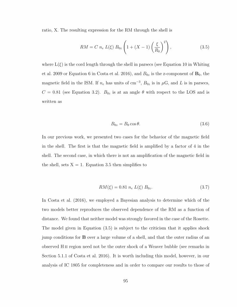
ratio, X. The resulting expression for the RM through the shell is

RM = C ne L(ξ) B0z

(1 + (X − 1)

(ξ

R0

)2), (3.5)

where L(ξ) is the cord length through the shell in parsecs (see Equation 10 in Whiting

et al. 2009 or Equation 6 in Costa et al. 2016), and B0z is the z-component of B0, the

magnetic field in the ISM. If ne has units of cm−3, B0z is in µG, and L is in parsecs,

C = 0.81 (see Equation 3.2). B0z is at an angle θ with respect to the LOS and is

written as

B0z = B0 cos θ. (3.6)

In our previous work, we presented two cases for the behavior of the magnetic field

in the shell. The first is that the magnetic field is amplified by a factor of 4 in the

shell. The second case, in which there is not an amplification of the magnetic field in

the shell, sets X = 1. Equation 3.5 then simplifies to

RM(ξ) = 0.81 ne L(ξ) B0z. (3.7)

In Costa et al. (2016), we employed a Bayesian analysis to determine which of the

two models better reproduces the observed dependence of the RM as a function of

distance. We found that neither model was strongly favored in the case of the Rosette.

The model given in Equation (3.5) is subject to the criticism that it applies shock

jump conditions for B over a large volume of a shell, and that the outer radius of an

observed H ii region need not be the outer shock of a Weaver bubble (see remarks in

Section 5.1.1 of Costa et al. 2016). It is worth including this model, however, in our

analysis of IC 1805 for completeness and in order to compare our results to those of

95

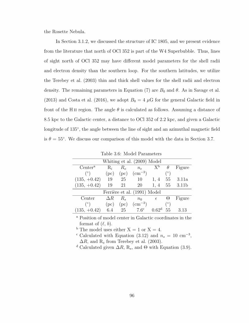
the Rosette Nebula.

In Section 3.1.2, we discussed the structure of IC 1805, and we present evidence

from the literature that north of OCl 352 is part of the W4 Superbubble. Thus, lines

of sight north of OCl 352 may have different model parameters for the shell radii

and electron density than the southern loop. For the southern latitudes, we utilize

the Terebey et al. (2003) thin and thick shell values for the shell radii and electron

density. The remaining parameters in Equation (7) are B0 and θ. As in Savage et al.

(2013) and Costa et al. (2016), we adopt B0 = 4 µG for the general Galactic field in

front of the H ii region. The angle θ is calculated as follows. Assuming a distance of

8.5 kpc to the Galactic center, a distance to OCl 352 of 2.2 kpc, and given a Galactic

longitude of 135, the angle between the line of sight and an azimuthal magnetic field

is θ = 55. We discuss our comparison of this model with the data in Section 3.7.

Table 3.6: Model Parameters

Whiting et al. (2009) ModelCentera Ri Ro ne Xb θ Figure

() (pc) (pc) (cm−3) ()(135, +0.42) 19 25 10 1, 4 55 3.11a(135, +0.42) 19 21 20 1, 4 55 3.11b

Ferriere et al. (1991) ModelCenter ∆R Rs n0 ε Θ Figure

() (pc) (pc) (cm−3) ()(135, +0.42) 6.4 25 7.6c 0.62d 55 3.13a Position of model center in Galactic coordinates in the

format of (`, b).b The model uses either X = 1 or X = 4.c Calculated with Equation (3.12) and ns = 10 cm−3,

∆R, and Rs from Terebey et al. (2003).d Calculated given ∆R, Rs, and Θ with Equation (3.9).

96

(a)

(b)

Figure 3.11: Plots of LOS versus distance with the Whiting et al. (2009) model forX = 4 (solid) and X = 1 (dashed) for b < +0.9 using (a) the thick shell and (b) thethin shell parameters from Terebey et al. (2003). The background RM = –100 radm−2 from the Van Eck et al. (2011) model. See Table 3.6 for model parameters.

3.6.2 Analytical Approximation to Magnetized Bubbles of Ferriere et al. (1991)

Ferriere et al. (1991) presented a semi-analytic discussion of the evolution of

a stellar bubble in a magnetized interstellar medium. The theoretical object dis-

cussed by Ferriere et al. (1991) could describe a shock wave produced by a supernova

explosion or energy input due to a stellar wind. The main features of the model

were an outer boundary (e.g. outer shock) which was the first interface between the

undisturbed ISM and the bubble, and an inner contact discontinuity between ISM

material, albeit modified by the bubble, and matter that originated from the central

star or star cluster.

97

The main feature of the model is that plasma passing through the outer bound-

ary is concentrated in a region between the outer boundary and the contact discon-

tinuity. In what follows, we will refer to this region as the shell of the bubble. The

equation of continuity then indicates that there will be higher plasma density in the

shell, and the law of magnetic flux conservation indicates that there will be an in-

crease in the strength of the magnetic field in the shell relative to the general ISM field.

Ferriere et al. (1991) were interested in the structure of the bubble, and their results

have been corroborated by the fully numerical studies of Stil et al. (2009). However,

Ferriere et al. (1991) did not calculate the Faraday rotation measure through their

model for diagnostic purposes. Stil et al. (2009) explicitly considered the model RMs

from their calculations, but only for a couple of cases and for two values of bubble

orientation. It is our goal in this section to use a simplified, fully analytic approxi-

mation to the results of Ferriere et al. (1991), that permit RM profiles RM(ξ) for a

wide range of bubble parameters and orientation with respect to the LOS.

The geometry of the bubble is shown in Figure 3.12, which is an adaptation of

Figure 1 and Figure 4 from Ferriere et al. (1991). An important feature of Figure

3.12, not present in Ferriere et al. (1991), is the orientation of the line of sight at

an angle Θ with respect to the ISM magnetic field at the position of the bubble,

and the impact parameter ξ indicating the separation of the LOS from the center

of the bubble. The region interior to the contact discontinuity is referred to as the

cavity, and for the purposes of our discussion will be considered a vacuum. A major

simplification that we adopt, based on an approximation to the results of Ferriere

et al (1991), is that the magnetic field in the shell (Bs) is entirely in the azimuthal

direction, and that we ignore radial variations within the shell, i.e.

Bs(r, θ) ≡ ±Bs(θ)eθ (3.8)

98

Figure 3.12: Illustration of the shell and cavity produced by a stellar wind, as de-scribed by Ferriere et al. (1991). The z direction is that of the interstellar magneticfield, and Θ is the angle between the magnetic field and the line of sight. The line ofsight passes at a closest distance ξ from the center of the cavity (the “impact param-eter”). Other parameters in the figure are defined in the text. Figure adapted fromFigure 1 or Figure 4 of Ferriere et al. (1991).

where eθ is a unit vector in the azimuthal direction, and the ± is selected by the

polarity of the interstellar field at the bubble.

To calculate the Faraday rotation through the shell of the bubble, we need ns

(the electron density in the shell) and Bs as a function of the angular coordinate θ,

as well as the geometry of the line of sight. We also need expressions for the outer

radius, Rs(θ), and thickness of the shell. This information is given by three equations

in Ferriere et al. (1991). The shell thickness ∆R is given by Equation (46) of Ferriere

et al. (1991), (∆R

Rs

)=

1

2ε sin θ (3.9)

This equation introduces the important dimensionless parameter ε, a measure of

the relative thickness of the shell. In the analysis that follows, we consider it a

parameter that can be adjusted to the observations. Ferriere et al. (1991) stress that

99

this expression breaks down near the “poles” of the bubble. Ferriere et al. (1991) give

the conditions necessary for its validity, and it applies through most of the bubble.

The condition of magnetic flux conservation in the plasma swept up into the

shell gives the following expression for the strength of the magnetic field,

Bs(θ) =1

2

(Rs

∆R

)B0 sin θ (3.10)

This is Equation (40) of Ferriere et al. (1991), and B0 is the magnitude of the magnetic

field in the external ISM. Strictly speaking, the RHS of our Equation (3.10) gives

the θ component of Bs in Equation (40) of Ferriere et al. (1991), but given the

approximation of Equation (3.8), our Equation (3.10) is self-consistent.

Our final equation for the plasma properties in the shell gives the mass density,

which accounts for the sweeping up and accumulation of mass in the shell,

ρs =1

3

(Rs

∆R

)ρ0 (3.11)

where ρ0 is the mass density in the unperturbed ISM. This is Equation (38) of Ferriere

et al. (1991). Approximating the plasma by fully ionized hydrogen, the shell and ISM

electron densities (ns and n0) are given by

ns =1

3

(Rs

∆R

)n0 (3.12)

3.6.2.1 RM Calculation for Lines of Sight Through Walls of Shell

In evaluating the integral Equation (3.1) or Equation (3.2) through the model

shell shown in Figure 3.12, we break the calculation into two parts, each with its own

approximations. The first calculation is for lines of sight that pass through a portion

of the shell, emerge into the cavity, and then reenter the shell on the opposite side

100

before exiting the shell entirely. This is the case illustrated in Figure 3.12. We adopt

the rough approximation

C

∫1

ns(s) Bs(s) · ds ' ± C ns(θ1) Bs(θ1) ∆s(θ1) [eθ · es] (3.13)

In what follows, we omit the ± in front of the RHS, with the understanding that the

polarity of the field in the shell is determined by the sign of the measured RM. On

the left hand side of the approximation, we introduce the variable s as a coordinate

along the line of sight; ds is an incremental vector along the line of sight from the

source to the observer, and es is the corresponding unit vector. The constant C is

the same as introduced in Equation (3.5). On the right side, we express the electron

density and magnetic field strength as functions only of the polar angle θ. ∆s is the

thickness of the shell along the line of sight, shown in Figure 3.12 with the gray solid

line segments, and the subscript “1” indicates the first section of the shell that is

transited by the line of sight.

Straightforward algebraic manipulations can be used to evaluate this expression,

given relations (3.8) - (3.12), and we obtain the following result for the RM through

one of the segments through the shell,

RM1 =Cn0B0Rs

3ε

ξ√R2s − ξ2

(3.14)

RM1 =Cn0B0Rs

3ε

x√1− x2

(3.15)

where we introduce a variable x ≡ ξRs

, and by Rs we mean Rs(θ1), θ1 being the

polar angle at which the LOS enters the shell on the side facing the observer (see

Figure 3.12). Obtaining Equation (3.15) from Equation (3.14) requires use of the

approximation Rs(θ⊥) ' Rs(θ1).

101

The contribution from the second passage through the shell gives a similar term,

and the total RM is the sum of these. One simple case is when the two contributions

are approximately equal, so we have a rough expression for the total RM

RM =2Cn0B0Rs

3ε

x√1− x2

(3.16)

This is one of the equations we shall compare to our data.

There is an interesting opposite extreme for the value of total RM. If the angle

Θ is sufficiently large, one of the shell transits will be in the upper half plane, and the

other will be in the lower half plane. In this case, the projection of the shell magnetic

field on the line of sight will be the opposite in the two segments. What is happening

is that in one half of the shell (say that facing the observer), the ISM magnetic field

is rotated towards the observer, while in the opposite shell (e.g. back wall of shell)

the ISM field is rotated away. If the magnitude of the RM in the two portions of the

LOS are equal, the RM from the facing shell transit will be opposite and equal to

that from the rear portion. In this case, the total RM is zero. This fact can be easily

grasped by imaging a line of sight with Θ = π2.

The rough model presented in this section can therefore account for one of the

striking results from Stil et al. (2009). For his model shell, motivated by the work of

Ferriere et al. (1991), the RM is very large when the LOS is parallel to the interstellar

magnetic field (Θ = 0). However, when the LOS is perpendicular, (Θ = π2), the

RM is small and fluctuates between positive and negative values, presumably due to

instabilities in the shell, which can be present in the simulation studies of Stil et al.

(2009).

The conditions for this to occur depend on Θ and ξ. It can be shown that there

102

is a critical value of x = ξRs(θ)

, xc,

xc = sin Θ. (3.17)

If x ≥ xc, then the RM contributions from the two parts of the shell have the same

sign, and Equation (3.16), or a generalization of Equation (3.14) or (3.15) holds. If

x < xc, the RM contributions from the two portions of the shell are of opposite sign,

and the total RM could be zero.

3.6.2.2 RM for Lines of Sight Entirely Within the Shell

If the “impact parameter” ξ is sufficiently large, the entire line of sight is within

the shell from the point of ingress to that of egress. It can be shown that this occurs

for x ≥ xmin, with

xmin = 1− 1

2ε cos Θ (3.18)

and the circumstances can be visualized by reference to Figure 3.12. In this case, the

rough approximation embodied in Equation (3.13) needs to be replaced by an integral

over the line of sight from the ingress point to the egress point. This can be done by

changing the variable of integration from s (a coordinate along the line of sight) to

the polar coordinate θ, and the integral in Equation (3.13) is integrated from θ1, the

ingress point (see Figure 3.12), to θ⊥ (point of closest approach of the LOS to the

center of the bubble) and then to θ2, the egress point.

After a reasonable amount of algebra, it can be shown the contribution RM1,

consisting of that part of the RM from θ1 − θ⊥, is given by

RM1 =2Cn0B0ξ

3ε2

∫ θ⊥

θ1

dθ

sin θ sin(Θ− θ)(3.19)

The integral in Equation (3.19) depends on Θ, and via θ1 = θ1(x), on x or ξ. It can

103

be recast in the form

RM1 =2Cn0B0Rs

3ε2

[x

∫ π/2

φ1(x)

dA

sin(A+ Θ) sinA

](3.20)

φ1(x) = arcsin

(ξ

Rs(θ1)

)(3.21)

If one makes the brutal assumption that the RM on the second half of the

integration through the shell, RM2 is approximately the same as RM1, and adopts a

first order approximation that Rs is independent of θ, so that x = ξRs

, we have the

following approximate expression for the total RM in the outer parts of the shell.

These are lines of sight for which x > xmin.

RM =4Cn0B0Rs

3ε2

[x

∫ π/2

φ1(x)

dA

sin(A+ Θ) sinA

](3.22)

φ1(x) = arcsin(x) (3.23)

The integral in Equation (3.22) can be readily evaluated via a Mathematica

notebook or a Python code. Equations (3.16) and (3.22) and (3.23) comprise our

rough analytic model for the RM(ξ) throughout the shell. The expression depends

on the parameters Rs, ε, Θ, n0, and B0. Another parameter that must be specified

when comparing the model to data is the background Galactic RM, RMoff .

A plot of the expressions which utilize Equations (3.16), (3.22), and (3.23) is

shown in Figure 3.13, for a representative set of parameters for IC 1805 (see Table 3.6).

The values of ε and n0 are calculated using Equations (3.9) and (3.12), respectively,

given the electron density in the shell, the thickness of the shell, and the outer shell

radius from the thick shell approximation in Terebey et al. (2003). We utilize the

same value of Θ, B0, and RMoff as in Section 3.6.1. The dashed line is the expression

104

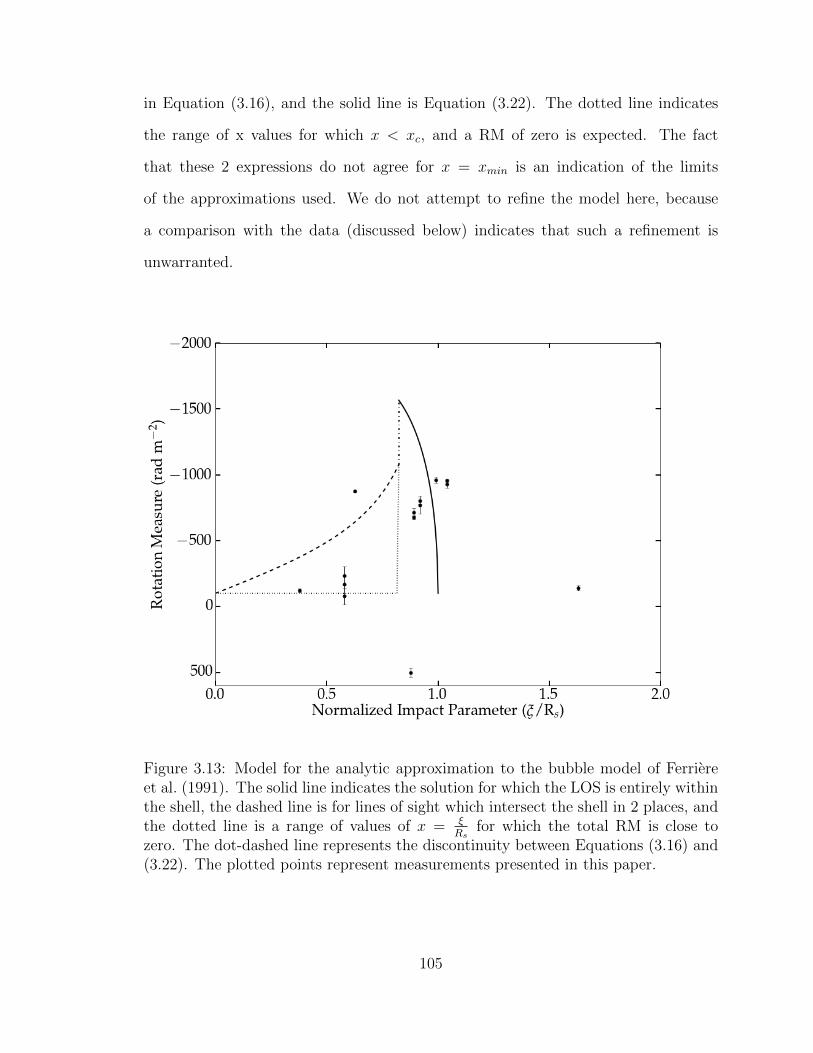
in Equation (3.16), and the solid line is Equation (3.22). The dotted line indicates

the range of x values for which x < xc, and a RM of zero is expected. The fact

that these 2 expressions do not agree for x = xmin is an indication of the limits

of the approximations used. We do not attempt to refine the model here, because

a comparison with the data (discussed below) indicates that such a refinement is

unwarranted.

Figure 3.13: Model for the analytic approximation to the bubble model of Ferriereet al. (1991). The solid line indicates the solution for which the LOS is entirely withinthe shell, the dashed line is for lines of sight which intersect the shell in 2 places, andthe dotted line is a range of values of x = ξ

Rsfor which the total RM is close to

zero. The dot-dashed line represents the discontinuity between Equations (3.16) and(3.22). The plotted points represent measurements presented in this paper.

105

3.7 Discussion of Observational Results

3.7.1 Comparison of Models with Observations in the H ii Region

In this section we discuss the results of the two models presented in Sections

3.6.1 and 3.6.2. In both cases, we adopt the Terebey et al. (2003) center for geometric

ease and spherical symmetry as well as the parameters given in their Table 3 for a

thick shell.

Figures 3.11a and 3.11b show model RM values for lines of sight south of IC

1805 (b < 0.9) with the Whiting et al. (2009) model for the RM as a function of

distance and the shell parameters from Terebey et al. (2003). Table 3.6 gives the

values of the center of the bubble, the shell radii, the electron density, X, and θ for

Figure 3.11. Neither model reliably reproduces the observed RM as a function of

distance, and as in Costa et al. (2016), the model cannot account for the dispersion

of RM values at similar distances. Generally, the lines of sight in the cavity are low

and are more consistent with the background RM. In the thin shell approximation,

the largest RM values are associated with lines of sight outside the shell. While the

model without amplification of the magnetic field in the shell can marginally account

for the magnitude of the RM, the model with amplification (Equation 3.5) predicts far

too high values for the RM for θ = 55. The analysis contained here mildly supports

a result from Costa et al. (2016) for the Rosette Nebula; Faraday rotation values

through these H ii regions do not permit a substantial increase in |B| over the general

Galactic field.

To reproduce the observed RM in the shell at ξ ∼ 20 pc, the angle between the

magnetic field and the observer would need to be tilted more into the plane of the

sky for the X = 4 case or into the line of sight for the X =1 case. For the former

case, an angle ∼ 75 would reproduce the magnitude of the RM in the shell; such an

106

angle is greater than that expected from a geometric argument, even accounting for

a magnetic field pitch angle of ∼ 8. Also, no one angle can account for the range of

the RM values in the cavity.

From our analytical solution for the RM due to a magnetized bubble with

solutions from Ferriere et al. (1991), we can approximate the behavior of the RM for

different values Θ. As stated in Section 3.6.1, a geometric approach gives Θ = 55.

As seen in Figure 3.13, the model overestimates the value of the RM in the shell and

performs poorly in the cavity. To reproduce the magnitude of the observed RMs in

the shell, the magnetic field would need to be bent more into the line of sight.

Stil et al. (2009) carried out numerical MHD simulations of the Ferriere bubbles,

which are obviously more accurate than our analytic approximations. Furthermore,

they specifically consider and calculate the Faraday rotation through their models.

However, Stil et al. (2009) only consider Θ = 0 and Θ = 90, so the calculations

reported in that paper can not explore the changes in RM structure with Θ. Further-

more, the Faraday rotation calculation of Stil et al. (2009) is done when the outer

radius Rs ∼ 200 pc (see Figure 14 of Stil et al. 2009), which is much larger than the

structure we are modeling in Section 3.6.2 of this paper. In what follows, we compare

our observations with the results presented in Section 6 of Stil et al. (2009).

If LOS || Bext, then the highest values of RM will be through the shell closest

to the Galactic plane, but the mean RM across the region will be similar to the mean

RM exterior to the bubble (see Figure 14 of Stil et al. 2009). Out of the Galactic

plane, the RM is 20 – 30% of the mean RM exterior to the bubble. Effectively, the

largest RMs will always be found in the Galactic plane, and different lines of sight

through the bubble will have varying RM values.

In comparing the simulations of Stil et al. (2009) to our observational results,

we find low RM measures for lines of sight through the cavity, though not always

low (e.g., W4-I14 and -I17 vs -I15 and -I21). Lines of sight through the shell have

107

generally large RMs, which is inconsistent with a Bext perpendicular to the LOS. The

case of LOS || Bext is inconsistent as well because far from the bubble, the RM is

low (e.g., W4-O26 vs -I24) even at similar latitudes, and the lines of sight at b >

1 are consistent with the background RM instead of being reduced by 70 – 80%.

Unsurprisingly, our results indicate a case somewhere between these two predictions.

As a reminder, we note that the largest values of the RM are for lines of sight exterior

to the shell, which is not a prediction from Stil et al. (2009), most likely due to their

simulations modeling the ionized bubble and not a PDR structure.

3.7.2 Magnetic Fields in the PDR

In Section 3.5.3, we examine evidence for a PDR outside the southern loop of IC

1805. Brogan et al. (1999), Troland et al. (2016), and Pellegrini et al. (2007) report

large (∼ 150 µG) magnetic fields in PDRs associated with the Orion Veil and M17.

In the analysis that follows, we attempt to understand the large RM values for lines

of sight through the IC 1805 PDR.

If we consider the PDR and the H ii region to be in pressure equilibrium and

include magnetic pressure in the PDR, then

PH iith = PPDR

th + PPDRmag , (3.24)

where PH iith and PPDR

th are the thermal pressures in the H ii region and PDR, re-

spectively, and PPDRmag = B2

8πis the magnetic pressure in the PDR. In the H ii region,

PH iith = 2nH ii

e k TH ii, where nH iie and TH ii are the electron density and temperature,

k is the Boltzmann constant, and the factor of 2 accounts for the contribution from

both ions and electrons. For PPDRth = NPDR k TPDR, NPDR and TPDR are the neutral

hydrogen density and the temperature in the PDR.

Near the interface of the PDR and the H ii region, the electron density in the

108

PDR is governed by photoioniziation of carbon (Tielens & Hollenbach, 1985), so we

estimate nPDRe by

nPDRe = NPDRXC ,

where XC is the cosmic abundance of carbon given in Table 1.4 of Draine (2011) (XC

∼ 2.95 × 10−4). Solving for B in Equation (3.24) gives

B =√

8π k(2 nH iie TH ii −NPDR TPDR), (3.25)

and inserting it into Equation (3.2), we express the RM in the PDR as

RM = 0.81 L XCNPDR

√8π k (2 nH ii

e TH ii −NPDR TPDR). (3.26)

We differentiate Equation (3.26) with respect to NPDR to find the value of NPDR that

maximizes the RM, which is

NPDR =4

3

nH iie TH ii

TPDR

. (3.27)

Inserting values of TH ii = 8000 K, nH iie = 10 cm−3 (Terebey et al., 2003), and TPDR

= 100 K (Tielens & Hollenbach, 1985), gives NPDR ∼ 1000 cm−3, B ∼ 14 µG (Eq

3.25), and RM ∼ 100 rad m−2. The electron density in the H ii region is governing

the maximum B expected in the PDR given pressure balance. For the IC 1805 H ii

region, ne is low compared to M17 (ne ∼ 560 cm−3) (Pellegrini et al., 2007), which

suggests that a high density (pressure) H ii region is needed to explain large magnetic

fields in the PDR.

We now consider what values of the RM we might expect in the PDR given

magnetic fields strengths of ∼ 100 µG. Assuming thermal pressure balance (PH iith =

PPDRth ) only, then NPDR = 200 NH ii

H , where NH iiH is the neutral hydrogen in the dust

109

shell of the H ii region. Using NH iiH = 4.8 cm−3 from Table 2 of Terebey et al. (2003)

for the dust shell, nPDRe = 200 NH ii

H XC . For a 100 µG field in the PDR, RM ∼ 700

rad m−2, assuming L ∼ 30 pc. This is the same magnitude of the RM we find for

W4-I2, -I6, and -I24 in the IC 1805 PDR.

Our analysis suggests that a simple pressure balance analysis predicts low RM

values from the PDR that are inconsistent with our observations. Terebey et al.

(2003) discuss an extended halo of ionized emission around the southern loop, which

may indicate that there are more free electrons present outside the obvious ionized

shell as seen in Figure 3.2. This may account for the larger values of the RM we

observe. It is clear that knowing the electron density in this region and determining

the presence of a PDR through observations, such as carbon radio recombination

lines, is necessary to understand how the magnetic field is modified in this complex

region.

3.8 A Comparison of IC 1805 and the Rosette Nebula as “Rotation Mea-

sure Anomalies”

We are interested in how the Galactic magnetic field is modified by OB associa-

tions via their stellar winds and ionizing photons, and we started our study with the

Rosette Nebula, where we found large (∼ 103 rad m−2) RM measurements through

the ionized shell of the H ii region (Costa et al., 2016).

In the case of the Rosette, we find positive RM across the region, and for IC

1805, we find negative values. If the Galactic magnetic field follows the spiral arms

in a clockwise direction, then we would expect the LOS magnetic field component to

be pointed towards us (positive B) for ` > 180, and pointed away from us (negative

B) for ` < 180. Except for one line of sight in each nebula, we find that the polarity

of the Galactic magnetic field is preserved across each nebula and is consistent with

110

Table 3.7: Stellar ParametersStar Cluster Star Type M V∞ LW=1

2Mv2

∞a

(Myr−1) (km/s) (erg s−1)

NGC 2244

HD 46223 O4V(f)b 1.6×10−6 c 3100d 4.8×1036

HD 46150 O5.5Ve 2.0×10−6 c 3100d 6.0×1036

HD 46202 O9V(f)b 6.3×10−8 c 1150d 2.6×1034

HD 46149 O8.5V(f)b 2.0×10−7 c 1700f 1.8×1035

OCl 352HD15570 O4Ib 1.0×10−5 c 2200g 1.5×1037

HD15558 O4IIIb 6.3×10−6 c 3000f 1.8×1037

HD 15629 O5Vb 2.0×10−6 c 2900h 5.3×1036

a Calculated mechanical wind luminosity based on cited mass loss ratesand terminal velocities.

b Massey et al. (1995)c Howarth & Prinja (1989)d Chlebowski & Garmany (1991)e Roman-Zuniga & Lada (2008)f Garmany (1988)g Bouret et al. (2012)h Groenewegen et al. (1989)

the large scale field through the arm.

In our study of the Rosette, we investigated whether the magnetic field is am-

plified in the shell of the nebula. We found that the model without amplification

was weakly favored over the case when the magnetic field is amplified in the shell.

When we applied the same model to IC 1805, however, it is difficult to conclude in

favor of either model, but in both cases, the model with an enhanced magnetic field

over predicts the RM. From inspection of Figures 3.11a and 3.11b, it seems that the

model without amplification better accounts for the magnitude of the observed RMs,

the observations do not conform to the model prediction of RM(ξ), and the model

cannot account for the wide range in observed values of RM at a given ξ.

In the present study, we find the highest RMs for lines of sight outside the

obvious shell structure, though one line of sight (W4-I13) does appear to intersect

the ionized shell and it has a large RM. These lines of sight may be probing the

111

magnetic field within the PDR. In the case of the Rosette, we found that the highest

RM values were for lines of sight through the bright ionized shell. However with our

work on IC 1805 and the PDR associated with it, we have briefly revisited our results

in the Rosette, particularly Figure 1 from Costa et al. (2016). There are a few lines

of sight with RM of order a few 102 rad m−2 that appear to be outside the ionized

shell. These lines of sight were included in the background estimate for the Rosette,

but if the Rosette also has a PDR, then these lines of sight may actually be probing

that material.

Table 3.7 lists spectral type, mass loss rate, terminal wind velocity, and calcu-

lated wind luminosity from the literature for O stars with the largest wind luminosities

in both NGC 2244, which is associated with the Rosette Nebula, and OCl 352. The

sum of the wind luminosities of the three main stars in OCl 352 is 3.8 × 1037 ergs

s−1, while the corresponding number for NGC 2244 (4 stars) is 1.1 × 1037 ergs s−1. In

addition, OCl 352 appears to have more luminous stars. As such, OCl 352 might be

expected to produce a more energetic stellar bubble than NGC 2244. Our Faraday

rotation measurements show no indication of this, in that the largest RMs observed

are similar for the two objects. In fact, higher RMs were measured for the Rosette

than for any line of sight through IC 1805. A number of factors can control the

impact a star cluster has on the ISM. If some relationship exists between the total

wind luminosity of a star cluster and properties of an interstellar bubble that can be

measure with Faraday rotation, it will apparently require a large sample of clusters/

H ii regions to reveal it.

3.9 Future Research

In the future, we will continue our investigation of H ii regions and how they

modify their surroundings and the Galactic magnetic field. An immediate investiga-

tion will be centered on observations of the H ii region IC 1396. This will provide a

112

third H ii region with different age, stellar content, and Galactic location. The obser-

vations are similar to those we have made of the Rosette Nebula and IC 1805. The

observations of IC 1396 have been made with the VLA and are awaiting analysis. By

adding more H ii regions to our study, we can begin to address questions such as

1. Since the electron density distributions in H ii regions are known from radio

continuum observations, we can inquire what conditions would result in an RM

>> 103 rad m−2 through the shell of an H ii region.

2. Is it a general property of H ii regions and stellar bubbles that the polarity of

the Galactic magnetic field is preserved within the region? The answer to this

question has implications for the amplitude of MHD turbulence in the ISM on

scales of the order of the H ii regions, ∼ 10− 30 pc.

3. Do PDRs around other nebulae produce high RMs? What is the magnitude of

the RM due to the PDR relative to that of the shell of an H ii region?

In addition to increasing the number of H ii regions, understanding Faraday complex-

ity and how to interpret the associated RM measurements is important to studies

of Galactic magnetic fields, particularly with large polarization surveys like the VLA

Sky Survey (VLASS) and Polarisation Sky Survey of the Universe’s Magnetism (POS-

SUM) with the Australian Square Kilometre Array Pathfinder (ASKAP) in the near

future.

3.10 Summary and Conclusions

1. We performed polarimetric observations using the VLA for 27 lines of sight

through or near the shell of the H ii region and stellar bubble associated with

the OB association OCl 352.

2. We obtain RM measurements for 20 sources using two methods. The first is

113

through the traditional least-squares fit to χ(λ2), and the second is using RM

Synthesis. Including components that are resolved, we report 27 RM values,

and we find good agreement between the two methods. We find the same sign

of the RM across the entire region with the exception of one source, W4-I18.

We estimate a background RM due to the general ISM of –145 rad m−2 in this

part of the Galactic plane. We measure an excess of RM of ∼ +600 to –800 rad

m−2 due to W4.

3. Only one line of sight has a positive RM value, W4-I18. It has a RM of +501 ±

33 rad m−2, and it is located 5.6 arcminutes from the center of OCl 352. This line

of sight may be probing the material close to the massive stars. The orientation

of the line of sight component of the magnetic field is directed towards the

observer, whereas in the rest of the region, the magnetic field is directed away.

4. We find that some of the lines of sight with the largest RM values occur just

outside the obvious ionized shell of IC 1805 and are potentially probing the

magnetic field in the PDR. The lines of sight through the cavity of the bubble

have lower RM values than those through the shell. In the W4 Superbubble,

which is north of OCl 352, we find RM values consistent with the background

RM.

5. We discuss two shell models to reproduce the magnitude of the RM and its

dependency on distance from the center of the star cluster. We employed the

first of these models in Savage et al. (2013) and Costa et al. (2016), and it is

based on the Weaver et al. (1977) solution for a stellar bubble, which includes

a shock expanding into an ambient medium. The second model uses magnetic

flux conservation to describe how the magnetic field is modified in the shell

and consists of a simplified analytic approximation to the results presented

by Ferriere et al. (1991). Neither of these simplified models accounts for the

114

dependence of RM on spatial location. Both types of model have a dependence

of RM on ξ, the separation of the line of sight from the center of the nebula,

whereas the observations show a large range of RM for sources with similar

values of ξ.

6. Because we have independent information on the electron density from radio

continuum observations of both IC 1805 and the Rosette Nebula, out observa-

tions can limit the magnitude of the magnetic field in the H ii regions. Our RM

measurements indicate that the field does not greatly exceed the value in the

general ISM.

7. We compare our results from the current study of IC 1805 and our previous

study of the Rosette Nebula. Notably, we find the same order of magnitude for

the RM for the two nebulae, but the sign of the RM in each region is opposite.

Since IC 1805 and the Rosette are at different Galactic longitudes and on either

side of b = 180, the sign difference between the two nebula is consistent with

a Galactic magnetic field that follows the spiral arm structure in a clock-wise

direction, as suggested in models (Van Eck et al., 2011).

115

CHAPTER 4

SUPPORTING WORK

In this chapter, I present supporting work to the results and conclusions dis-

cussed in Chapters 2 and 3.

4.1 Analysis of Spectral Indices for Radio Sources

In Chapter 2, Section 2.3.1.2 and Chapter 3, Section 3.3.2, I introduce RM

Synthesis, which utilizes 4 MHz wide images in Stokes Q and U as inputs. Because

the “channel” mode of clean averages adjacent channels, it is necessary to correct

for the frequency dependence that can affect Q and U . The method I employ in

Costa & Spangler (2018) corrects Q and U at each frequency, ν, using the spectral

index (α). The flux densities, Sν , are determined using the CASA task imfit, which

fits a 2-D Gaussian to the intensity distribution of the source. The spectral index is

then determined by a least-squares fit to logSν versus log ν. I refer to these data as

“corrected” in the discussion that follows.

In general, the sources have spectral indices consistent with an optically thin

synchrotron spectrum. Figure 4.2a shows an example of such a spectrum for reference.

Tables 4.1 and 4.2 list spectral indices for the lines of sight through IC 1805 and the

Rosette, respectively. Figure 4.1 is a histogram of the spectral indices for the sources

in Tables 4.1 and 4.2, which has a distribution similar to that of radio galaxies from

Kellermann et al. (1969) (see their Figure 6) and more recently Franzen et al. (2014)

(see their Figure 5).

W4-I12, W4-O4, R-N4, R-N7, and R-N10L are sources that raise cautionary

flags. Figure 4.2 shows the spectra for these sources. W4-I12 and R-N10L have

spectral indices that are consistent with being flat, R-N7 is largely scatter, and R-N4

has a negative but small spectral index. W4-O4 has a spectral index that is negative

116

Table 4.1: Flux Densities for Lines of Sight through IC 1805Source S4.402GHz S7.697GHz S1.4GHz

a

α7.6974.402 χ2

νb

Name (mJy) (mJy) (mJy)

W4-I1 77.9 ± 1.4 70.4 ± 0.3 200 0.87 4.97W4-I2 10.6 ± 1.1 6.5 ± 0.6 181 0.97 0.17

W4-I2b 5.5 ± 0.2 3.1 ± 0.2 181 1.01 0.78W4-I3 82.6 ± 0.2 52.5 ± 0.1 169 0.86 40W4-I4 44.7 ± 2.6 24.9 ± 1.5 161 1.06 0.31

W4-I4b 41.3 ± 2.7 23.3 ± 1.8 161 1.01 0.27W4-I6 11.6 ± 0.7 6.2 ± 0.3 145 1.18 1.65W4-I8 47.3 ± 0.6 28.3 ± 0.5 111 0.95 0.3W4-I11 39.4 ± 0.4 22.3 ± 0.7 94 1.04 0.28W4-I12 77.9 ± 1.4 79.1 ± 2.0 63 -0.03 0.45W4-I13 16.5 ± 0.3 9.8 ± 0.3 54 0.96 0.82W4-I13b 5.6 ± 0.2 3.5 ± 0.2 54 0.84 0.42W4-I14 2.3 ± 0.1 1.3 ± 0.1 54 1.23 2.11W4-I14b 2.9 ± 0.1 1.6 ± 0.1 54 1.06 2.56W4-I15 27.2 ± 0.2 16.4 ± 0.3 52 0.91 0.21W4-I17 9.5 ± 0.4 4.8 ± 0.2 43 1.24 0.28W4-I17b 8.9 ± 0.3 5.4 ± 0.2 43 0.96 0.23W4-I18 24.5 ± 0.1 15.9 ± 0.2 42 0.77 1.79W4-I19 11.8 ± 0.6 10.4 ± 0.8 42 0.23 0.09W4-I21 5.7 ± 0.4 2.9 ± 0.3 32 1.09 0.24W4-I21b 5.2 ± 0.2 2.6 ± 0.2 32 1.10 0.60W4-I21c 16.0 ± 0.9 8.9 ± 0.5 32 1.11 0.12W4-I23 3.4 ± 0.4 1.1 ± 0.5 28 1.90 2.39W4-I23b 0.8 ± 0.1 0.2 ± 0.1 28 1.40 15.52W4-I24 20.4 ± 0.6 12.4 ± 0.9 72 0.94 0.06W4-I24b 12.6 ± 0.5 7.5 ± 0.5 72 1.01 0.23W4-O1 377.3 ± 0.8 229.8 ± 0.6 923 0.94 29.85W4-O2 107.0 ± 0.3 52.3 ± 0.1 406 1.34 29.55W4-O4 747.2 ± 4.1 792.1 ± 2.7 364 0.06 4.59W4-O5 94.5 ± 0.2 54.6 ± 0.2 245 0.94 2.02W4-O6 120.2 ± 0.2 81.7 ± 0.1 222 0.69 6.19W4-O7 52.2 ± 0.1 24.0 ± 0.1 196 1.40 6.75W4-O8 40.7 ± 0.1 1.3 ± 1.1 195 1.90 0.43W4-O10 64.9 ± 0.6 36.7 ± 3.1 174 1.04 0.06

a Flux densities retrieved from the NVSS catalog (Condon et al.,1998) at a resolution of 45 arcseconds.

b Reduced Chi-Squared of fit for log Sν vs log ν.

117

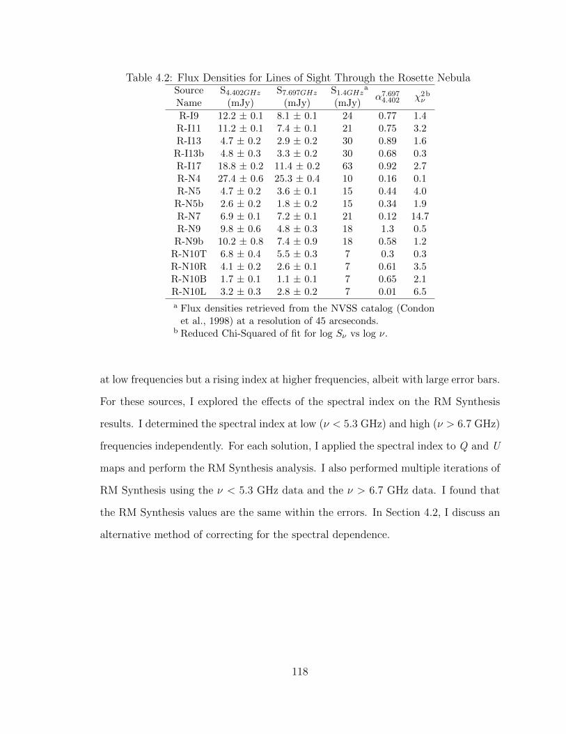
Table 4.2: Flux Densities for Lines of Sight Through the Rosette NebulaSource S4.402GHz S7.697GHz S1.4GHz

a

α7.6974.402 χ2

νb

Name (mJy) (mJy) (mJy)

R-I9 12.2 ± 0.1 8.1 ± 0.1 24 0.77 1.4R-I11 11.2 ± 0.1 7.4 ± 0.1 21 0.75 3.2R-I13 4.7 ± 0.2 2.9 ± 0.2 30 0.89 1.6R-I13b 4.8 ± 0.3 3.3 ± 0.2 30 0.68 0.3R-I17 18.8 ± 0.2 11.4 ± 0.2 63 0.92 2.7R-N4 27.4 ± 0.6 25.3 ± 0.4 10 0.16 0.1R-N5 4.7 ± 0.2 3.6 ± 0.1 15 0.44 4.0R-N5b 2.6 ± 0.2 1.8 ± 0.2 15 0.34 1.9R-N7 6.9 ± 0.1 7.2 ± 0.1 21 0.12 14.7R-N9 9.8 ± 0.6 4.8 ± 0.3 18 1.3 0.5R-N9b 10.2 ± 0.8 7.4 ± 0.9 18 0.58 1.2

R-N10T 6.8 ± 0.4 5.5 ± 0.3 7 0.3 0.3R-N10R 4.1 ± 0.2 2.6 ± 0.1 7 0.61 3.5R-N10B 1.7 ± 0.1 1.1 ± 0.1 7 0.65 2.1R-N10L 3.2 ± 0.3 2.8 ± 0.2 7 0.01 6.5

a Flux densities retrieved from the NVSS catalog (Condonet al., 1998) at a resolution of 45 arcseconds.

b Reduced Chi-Squared of fit for log Sν vs log ν.

at low frequencies but a rising index at higher frequencies, albeit with large error bars.

For these sources, I explored the effects of the spectral index on the RM Synthesis

results. I determined the spectral index at low (ν < 5.3 GHz) and high (ν > 6.7 GHz)

frequencies independently. For each solution, I applied the spectral index to Q and U

maps and perform the RM Synthesis analysis. I also performed multiple iterations of

RM Synthesis using the ν < 5.3 GHz data and the ν > 6.7 GHz data. I found that

the RM Synthesis values are the same within the errors. In Section 4.2, I discuss an

alternative method of correcting for the spectral dependence.

118

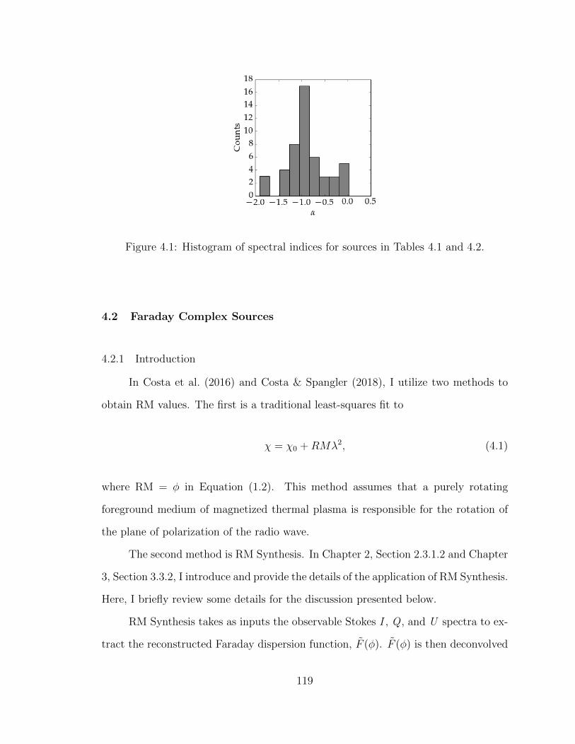
Figure 4.1: Histogram of spectral indices for sources in Tables 4.1 and 4.2.

4.2 Faraday Complex Sources

4.2.1 Introduction

In Costa et al. (2016) and Costa & Spangler (2018), I utilize two methods to

obtain RM values. The first is a traditional least-squares fit to

χ = χ0 +RMλ2, (4.1)

where RM = φ in Equation (1.2). This method assumes that a purely rotating

foreground medium of magnetized thermal plasma is responsible for the rotation of

the plane of polarization of the radio wave.

The second method is RM Synthesis. In Chapter 2, Section 2.3.1.2 and Chapter

3, Section 3.3.2, I introduce and provide the details of the application of RM Synthesis.

Here, I briefly review some details for the discussion presented below.

RM Synthesis takes as inputs the observable Stokes I , Q , and U spectra to ex-

tract the reconstructed Faraday dispersion function, F (φ). F (φ) is then deconvolved

119

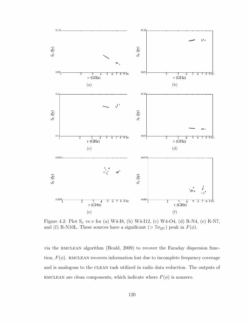
(a) (b)

(c) (d)

(e) (f)

Figure 4.2: Plot Sν vs ν for (a) W4-I8, (b) W4-I12, (c) W4-O4, (d) R-N4, (e) R-N7,and (f) R-N10L. These sources have a significant (> 7σQU) peak in F (φ).

via the rmclean algorithm (Heald, 2009) to recover the Faraday dispersion func-

tion, F (φ). rmclean recovers information lost due to incomplete frequency coverage

and is analogous to the clean task utilized in radio data reduction. The outputs of

rmclean are clean components, which indicate where F (φ) is nonzero.

120

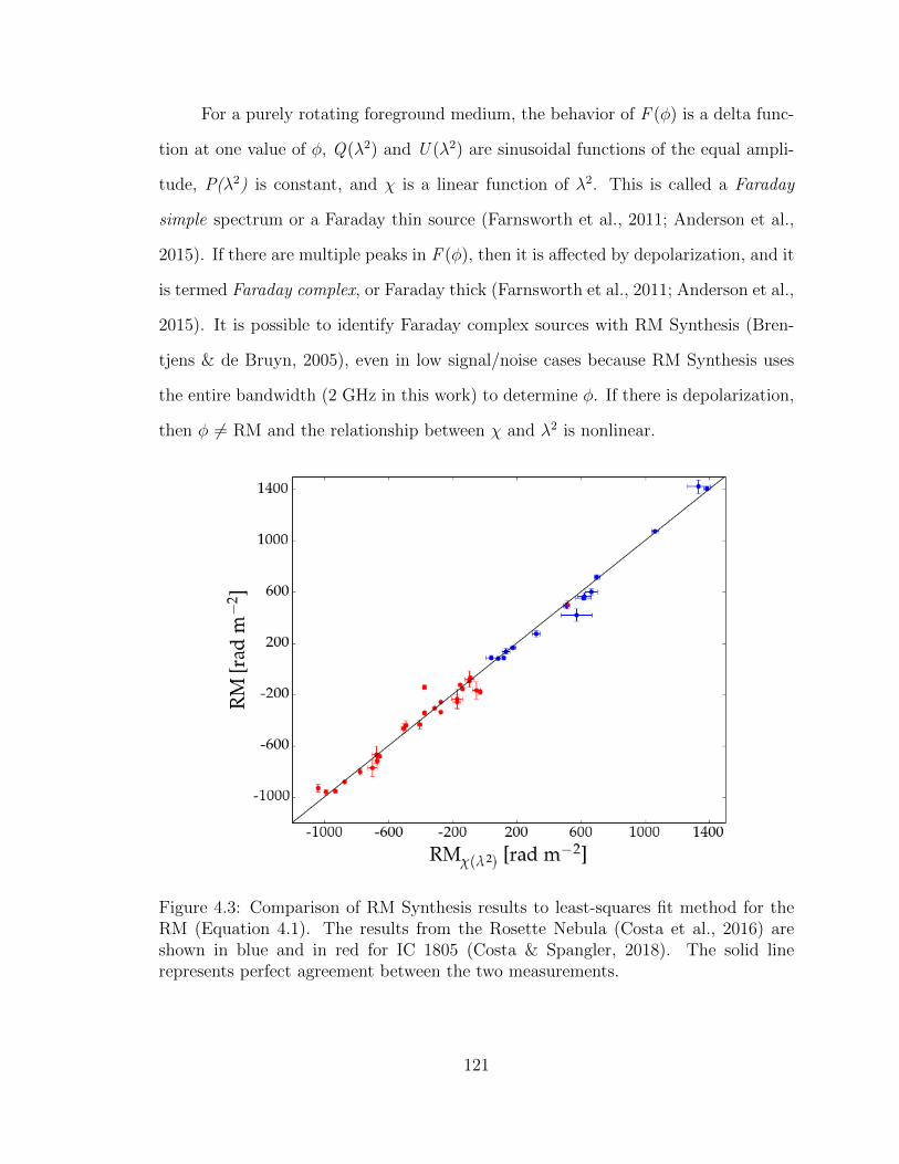
For a purely rotating foreground medium, the behavior of F (φ) is a delta func-

tion at one value of φ, Q(λ2) and U (λ2) are sinusoidal functions of the equal ampli-

tude, P(λ2) is constant, and χ is a linear function of λ2. This is called a Faraday

simple spectrum or a Faraday thin source (Farnsworth et al., 2011; Anderson et al.,

2015). If there are multiple peaks in F (φ), then it is affected by depolarization, and it

is termed Faraday complex, or Faraday thick (Farnsworth et al., 2011; Anderson et al.,

2015). It is possible to identify Faraday complex sources with RM Synthesis (Bren-

tjens & de Bruyn, 2005), even in low signal/noise cases because RM Synthesis uses

the entire bandwidth (2 GHz in this work) to determine φ. If there is depolarization,

then φ 6= RM and the relationship between χ and λ2 is nonlinear.

Figure 4.3: Comparison of RM Synthesis results to least-squares fit method for theRM (Equation 4.1). The results from the Rosette Nebula (Costa et al., 2016) areshown in blue and in red for IC 1805 (Costa & Spangler, 2018). The solid linerepresents perfect agreement between the two measurements.

121

Generally, I find good agreement for the RM between the two methods. Figure

4.3 compares the results of the RM Synthesis analysis to the least-squares fit to χ(λ2)

method for all sources in this thesis. In Costa et al. (2016) and Costa & Spangler

(2018), I do not find any sources with multiple peaks in F (φ), and I interpret the φ

from the RM Synthesis analysis as a characteristic RM of the source.

With large polarization surveys like the VLA Sky Survey (VLASS) and the

Polarisation Sky Survey of the Universe’s Magnetism (POSSUM) with the Australian

Square Kilometre Array Pathfinder (ASKAP), there is a lot of interest in identifying

and interpreting Faraday complex sources however. Anderson et al. (2015) report

in their study of 563 radio sources that at least 12% are Faraday complex, but they

warn that the number is likely higher given the limitation of the signal/noise in their

sample. Identification of Faraday complex spectra is an important step to extracting

magnetic field estimates from φ in a complex spectrum.

The conclusions of Farnsworth et al. (2011) and O’Sullivan et al. (2012) sug-

gest that RM Synthesis and rmclean alone are insufficient to determine φ if the

spectrum is Faraday complex. It is necessary to model the Q(λ2) and U (λ2) spectra

to determine the nature of a multi-peaked F (φ). The outputs of RM Synthesis and

rmclean, however, are useful in identifying Faraday complex spectra (Brown, 2011;

Law et al., 2011; Anderson et al., 2015) and as inputs to the QU analysis.

In the analysis that follows, I explore a Faraday complexity analysis for the lines

of sight in this thesis. In most cases, I do not expect departures from the conclusions

in Costa et al. (2016) and Costa & Spangler (2018), which discuss the modification

of the Galactic magnetic field through the shells of H ii regions. For some lines of

sight, the percent polarization (m) decreases as a function of λ2, which is an indicator

of depolarization, and these sources raised cautionary flags during the RM Synthesis

analysis. Additionally, there are some lines of sight that have multiple rmclean

clean components in a single F (φ) peak. Because QU modeling and RM Synthesis

122

are relatively new in practice, I explore a QU analysis in the sections below to gain

insight into the technique and Faraday complex spectra.

4.2.2 Depolarization Models

For the QU analysis, I utilize a Python program written by C. Purcell1 that uses

PyMultiNest (Buchner et al., 2014) to determine the best fit depolarization model.

PyMultiNest is a Python wrapper for MultiNest (Feroz et al., 2009), which is a Nested

sampling algorithm for Monte Carlo parameter estimation, and it utilizes Bayesian

analysis tools to perform model selection. The code takes as inputs Q(λ2), U (λ2),

and a function describing the depolarization.

Sokoloff et al. (1998) describe depolarization and provide mathematical repre-

sentations of many of the models discussed below. I briefly describe the models I

employ in the QU analysis here.

1. Faraday Thin. For a thin layer of a purely rotating medium of magnetized

thermal plasma, the complex polarized emission P is

P = p0 exp[2ı(χ0 +RMλ2)], (4.2)

where p0 is the intrinsic linear polarization, χ0 is the intrinsic polarization po-

sition angle, and λ is the wavelength (Eq 2; Sokoloff et al. 1998). Figure 4.4a is

a cartoon illustrating a configuration that produces a Faraday thin spectrum.

2. External Faraday Dispersion (EFD)/ Beam Depolarization. EFD occurs when

there are variations in the magnetic field (magnitude or direction) in a fore-

ground purely rotating screen within the beam of the antenna or when there are

multiple external purely rotating media with turbulent magnetic fields within

1Dr. Cormac Purcell is a lecturer in the Department of Physics and Astronomy at MacquarieUniversity. His RM Synthesis, RM Clean, and QU codes are available on github at https://

github.com/crpurcell/RM-tools.

123

a beam. Both are described by

P = p0 exp[−2σ2RMλ

4] exp[2ı(χ0 +RMλ2)], (4.3)

where σRM is the dispersion about the mean RM (Eq 21 of Burn 1966; Farnsworth

et al. 2011). Figure 4.4b is a cartoon schematic of beam depolarization.

3. Differential Faraday Rotation (DFR, uniform slab). Generally, DFR is due

to an external magnetized medium that is co-spatially emitting and rotating

radio waves. The radio waves on the far side of the slab will undergo a different

amount of Faraday rotation than those on the near side. This is Eq 3 of Sokoloff

et al. (1998)

P = p0sin(φλ2)

(φλ2)exp[2ı(χ0 +

1

2φλ2)]. (4.4)

Figure 4.4c is an example of a uniform slab.

4. Internal Faraday Dispersion. When a turbulent magnetized medium is co-

spatially emitting and rotating, then

P = p0 exp[2ıχ0]

(1− exp[2ıφλ2 − 2ξ2

RMλ4]

2ξ2RMλ

4 − 2ıφλ2

), (4.5)

where ξRM is the internal Faraday dispersion of the random field (Eq 18 of Burn

1966). Figure 4.4d is an example of internal Faraday dispersion.

Models may be added together to construct multicomponent models that de-

polarization effects along a line of sight (O’Sullivan et al., 2012). I restrict my QU

analysis to the following models and combinations of models.

1. One Faraday thin component (Equation 4.2).

2. One foreground screen (EFD) (Equation 4.3).

124

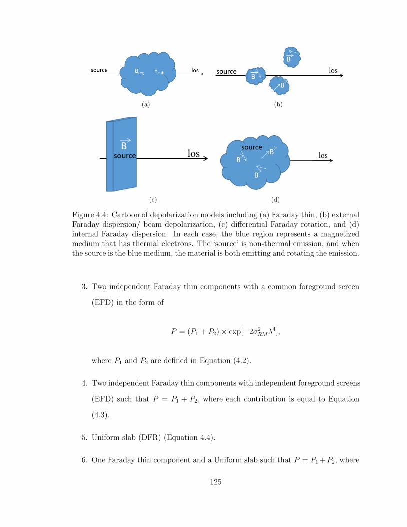
(a) (b)

(c) (d)

Figure 4.4: Cartoon of depolarization models including (a) Faraday thin, (b) externalFaraday dispersion/ beam depolarization, (c) differential Faraday rotation, and (d)internal Faraday dispersion. In each case, the blue region represents a magnetizedmedium that has thermal electrons. The ‘source’ is non-thermal emission, and whenthe source is the blue medium, the material is both emitting and rotating the emission.

3. Two independent Faraday thin components with a common foreground screen

(EFD) in the form of

P = (P1 + P2)× exp[−2σ2RMλ

4],

where P1 and P2 are defined in Equation (4.2).

4. Two independent Faraday thin components with independent foreground screens

(EFD) such that P = P1 + P2, where each contribution is equal to Equation

(4.3).

5. Uniform slab (DFR) (Equation 4.4).

6. One Faraday thin component and a Uniform slab such that P = P1 +P2, where

125

P1 is given by Equation (4.2) and P2 given by Equation (4.4).

7. Internal Faraday dispersion (Equation 4.5).

8. Two Faraday thin components such that P = P1 + P2, where each is given by

Equation (4.2).

While there are many combinations of models that could be tested, I restrict the

number of combinations to these models because they test for sources of depolarization

that would likely affect extragalactic sources with lines of sight through an H ii region.

Additionally, almost all of the sources in this work are extragalactic in nature and

are in the anti center of the Milky Way, which should reduce the number of rotating

media (e.g., other H ii regions) along the line of sight.

Farnsworth et al. (2011), O’Sullivan et al. (2012), Anderson et al. (2015), and

Pasetto et al. (2018) discuss and employ similar QU analyses for a number of lines

of sight; however, the lines of sight in this work are among the few that specifically

target the plasma shells of H ii regions. In the discussion that follows, I explore QU

analysis techniques using fractional and corrected Q and U values (see discussion

below) and the choice of channel width (e.g., 4 MHz) of the QU maps.

4.2.3 Results of the QU Analysis

I account for the frequency dependence that can independently affect Stokes Q

and U in two ways. The first method utilizes the spectral index of each source, the

center frequency νc, and the measured value of Q and U at each frequency, ν, to find

to find Qo and Uo using the relationship

Q = Qo

(ν

νc

)−αand U = Uo

(ν

νc

)−α.

126

I refer to these data as “corrected”. The second method utilizes fractional values of Q

and U , where q = Q/I and u = U/I, as the inputs to the QU analysis, and I refer to

these data as “fractional”. The fractional method is used in Farnsworth et al. (2011),

O’Sullivan et al. (2012), Anderson et al. (2015), and Pasetto et al. (2018), and I use

the corrected method in Costa et al. (2016) and Costa & Spangler (2018).

I also explore the effects of channel widths in the QU analysis. RM Synthesis

utilizes the entire bandwidth to calculate F (φ), and the input images in my analysis

have a channel width of 4 MHz, which is related to the maximum detectable Faraday

depth before bandwidth depolarization, |φmax| (Eq 63, Brentjens & de Bruyn 2005).

The modeling procedure may be adversely affected by low signal/noise due to the

small channel widths. The 4 MHz data have a maximum signal/noise ∼ 5 and, at

times, ∼ 1.

The other choice for the channel width is from the original CASA clean maps,

which are generated with the “mfs” mode in the clean task over the entire 128 MHz

bandwidth. The 128 MHz data typically have a signal/noise > 25 for the orthogonal

Stokes parameters, and only a few sources have signal/noise < 10. In addition, the

“mfs” mode takes into account the different (u, v) tracks corresponding to different

frequencies, and it determines and applies the spectral index correction to the source

during the clean task. Thus, these data are corrected.

The outputs of the QU analysis Python program are best fit parameters for

the selected depolarization model, the reduced χ2, the Bayesian information criterion

(BIC), and the Akaike information criterion (AIC). The Python program produces

plots of I vs ν, χ vs λ2, P, Q, and U vs λ2, and Q vs U. Additionally, it produces confi-

dence plots for the free parameters, which shows the posterior probability p(Mi|D, I),

where Mi is the model, D is the data, and I is a statement representing the prior

information and confidence intervals. For each free parameter in the model, there

is a corresponding histogram of the marginalized likelihood plotted on the diagonal.

127

Figure C.1 is an example of a triangular grid of the confidence plots.

I use the BIC to distinguish the more likely model; however, I also visually

inspect the model against the data and the corner plot to validate the selected model.

The results of the QU analysis can be placed into four categories, and Appendix

C, Figures C.1 – C.8 are representative plots of these categories using the fractional

data.

1. A poor fit (high BIC or AIC) to the data and/or no convergence in the posterior

probability (Figures C.1 & C.2).

2. A low BIC or AIC but a large reduced χ2 value, a poor visual fit, and no

convergence in the posterior probability. (Figures C.3 & C.4).

3. A good fit (low BIC or AIC) but multiple peaks in the posterior probability

(Figures C.5 & C.6).

4. A good fit (low BIC or AIC) and convergence in the posterior probability on a

single peak (Figures C.7 & C.8).

4.2.3.1 Results of 4 MHz Data

Selecting the best model is a difficult task for the 4 MHz data, as different

models have similar values of the BIC or AIC. For almost all of the sources, the Q

and U data are too compact, and the associated errors too large, to clearly identify

a good fit to the model. Figure 4.5a shows an example of this. The corrected and

fractional data are similarly affected, and for many parameters in the models, the

posterior probability does not converge to a value.

For W4-I1, -I3, -I8, and -I12, it is possible to identify at least three preferred

models that have a good fit (low BIC) and the posterior probability converges on

a single peak for the each parameter. Tables C.1 lists the preferred models, the

128

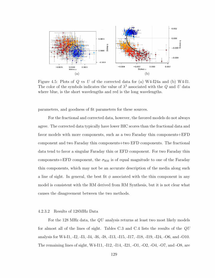
(a) (b)

Figure 4.5: Plots of Q vs U of the corrected data for (a) W4-I24a and (b) W4-I1.The color of the symbols indicates the value of λ2 associated with the Q and U datawhere blue, is the short wavelengths and red is the long wavelengths.

parameters, and goodness of fit parameters for these sources.

For the fractional and corrected data, however, the favored models do not always

agree. The corrected data typically have lower BIC scores than the fractional data and

favor models with more components, such as a two Faraday thin components+EFD

component and two Faraday thin components+two EFD components. The fractional

data tend to favor a singular Faraday thin or EFD component. For two Faraday thin

components+EFD component, the σRM is of equal magnitude to one of the Faraday

thin components, which may not be an accurate description of the media along such

a line of sight. In general, the best fit φ associated with the thin component in any

model is consistent with the RM derived from RM Synthesis, but it is not clear what

causes the disagreement between the two methods.

4.2.3.2 Results of 128MHz Data

For the 128 MHz data, the QU analysis returns at least two most likely models

for almost all of the lines of sight. Tables C.3 and C.4 lists the results of the QU

analysis for W4-I1, -I2, -I3, -I4, -I6, -I8, -I13, -I15, -I17, -I18, -I19, -I24, -O6, and -O10.

The remaining lines of sight, W4-I11, -I12, -I14, -I21, -O1, -O2, -O4, -O7, and -O8, are

129

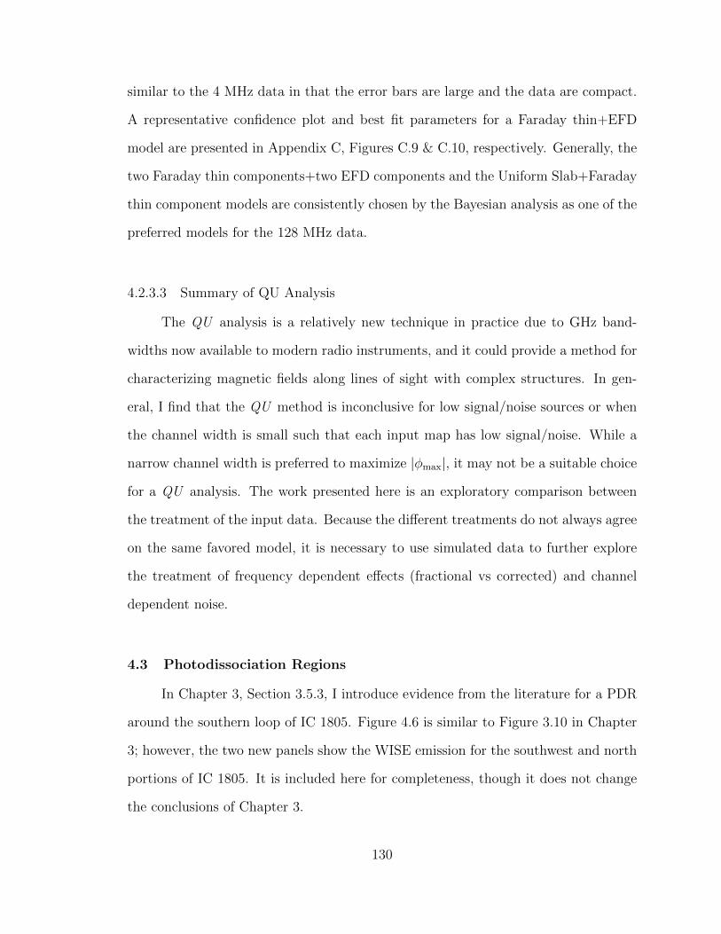
similar to the 4 MHz data in that the error bars are large and the data are compact.

A representative confidence plot and best fit parameters for a Faraday thin+EFD

model are presented in Appendix C, Figures C.9 & C.10, respectively. Generally, the

two Faraday thin components+two EFD components and the Uniform Slab+Faraday

thin component models are consistently chosen by the Bayesian analysis as one of the

preferred models for the 128 MHz data.

4.2.3.3 Summary of QU Analysis

The QU analysis is a relatively new technique in practice due to GHz band-

widths now available to modern radio instruments, and it could provide a method for

characterizing magnetic fields along lines of sight with complex structures. In gen-

eral, I find that the QU method is inconclusive for low signal/noise sources or when

the channel width is small such that each input map has low signal/noise. While a

narrow channel width is preferred to maximize |φmax|, it may not be a suitable choice

for a QU analysis. The work presented here is an exploratory comparison between

the treatment of the input data. Because the different treatments do not always agree

on the same favored model, it is necessary to use simulated data to further explore

the treatment of frequency dependent effects (fractional vs corrected) and channel

dependent noise.

4.3 Photodissociation Regions

In Chapter 3, Section 3.5.3, I introduce evidence from the literature for a PDR

around the southern loop of IC 1805. Figure 4.6 is similar to Figure 3.10 in Chapter

3; however, the two new panels show the WISE emission for the southwest and north

portions of IC 1805. It is included here for completeness, though it does not change

the conclusions of Chapter 3.

130

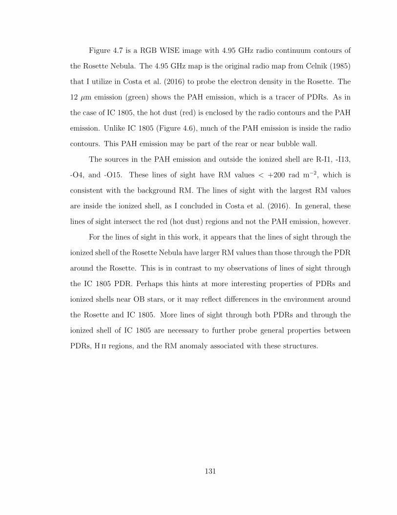
Figure 4.7 is a RGB WISE image with 4.95 GHz radio continuum contours of

the Rosette Nebula. The 4.95 GHz map is the original radio map from Celnik (1985)

that I utilize in Costa et al. (2016) to probe the electron density in the Rosette. The

12 µm emission (green) shows the PAH emission, which is a tracer of PDRs. As in

the case of IC 1805, the hot dust (red) is enclosed by the radio contours and the PAH

emission. Unlike IC 1805 (Figure 4.6), much of the PAH emission is inside the radio

contours. This PAH emission may be part of the rear or near bubble wall.

The sources in the PAH emission and outside the ionized shell are R-I1, -I13,

-O4, and -O15. These lines of sight have RM values < +200 rad m−2, which is

consistent with the background RM. The lines of sight with the largest RM values

are inside the ionized shell, as I concluded in Costa et al. (2016). In general, these

lines of sight intersect the red (hot dust) regions and not the PAH emission, however.

For the lines of sight in this work, it appears that the lines of sight through the

ionized shell of the Rosette Nebula have larger RM values than those through the PDR

around the Rosette. This is in contrast to my observations of lines of sight through

the IC 1805 PDR. Perhaps this hints at more interesting properties of PDRs and

ionized shells near OB stars, or it may reflect differences in the environment around

the Rosette and IC 1805. More lines of sight through both PDRs and through the

ionized shell of IC 1805 are necessary to further probe general properties between

PDRs, H ii regions, and the RM anomaly associated with these structures.

131

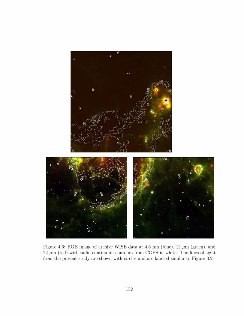
Figure 4.6: RGB image of archive WISE data at 4.6 µm (blue), 12 µm (green), and22 µm (red) with radio continuum contours from CGPS in white. The lines of sightfrom the present study are shown with circles and are labeled similar to Figure 3.2.

132

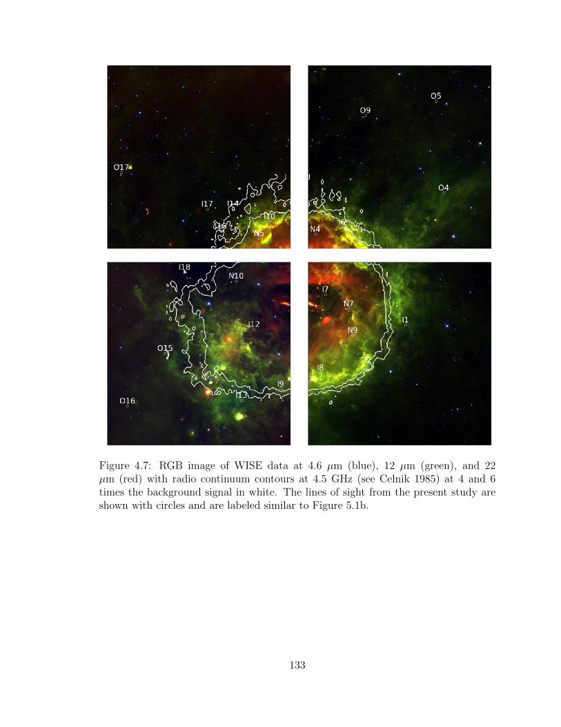
Figure 4.7: RGB image of WISE data at 4.6 µm (blue), 12 µm (green), and 22µm (red) with radio continuum contours at 4.5 GHz (see Celnik 1985) at 4 and 6times the background signal in white. The lines of sight from the present study areshown with circles and are labeled similar to Figure 5.1b.

133

4.4 Assessing Faraday Rotation and Nebular Properties from the Liter-

ature

In this section, I explore Faraday rotation results from the literature for H ii

regions and wind-blown bubbles. Table 4.3 list properties for 4 Faraday rotation

studies of H ii regions from the literature that report RM values for extragalactic

radio sources that have lines of sight that pass through or near to the H ii region.

These include the H ii regions from the study of Harvey-Smith et al. (2011), the

Gum Nebula, which Purcell et al. (2015) conclude is a wind-blown bubble and not

a supernova remnant, NGC 6334A (Rodrıguez et al., 2012), Sh2-232 (Heiles & Chu,

1980), Sh2-117, and Sh2-119 (Heiles et al., 1981).

The RM values in Harvey-Smith et al. (2011) and Purcell et al. (2015) are from

the Taylor et al. (2009) catalog, which utilized NVSS data to determine the RM values

for extragalactic radio sources. Because the Gum Nebula is ∼ 36 in size, there are

many lines of sight. The H ii regions in the Harvey-Smith et al. (2011) study have

between 5 and 50 lines of sight through the H ii region. There are only two lines of

sight through Sh2-232, Sh2-117, and Sh2-119, and only one measurement of +5100

± 900 rad m−2 for NGC 6334A (Rodrıguez et al., 2012).

Table 4.4 lists properties of these objects. Column one gives the astronomical

object, and columns two and three give the primary star responsible for the nebula

and the spectral type (if known), respectively. Column four gives the calculated wind

luminosities of the primary star, where Lw = 12M v2

∞. The mass loss rates, M , are

from Howarth & Prinja (1989), and the reference for the terminal wind velocities, v∞,

are noted in the table entry for Lw. The fifth column gives the diameter of the nebula.

Column six lists the maximum value of |RM| for lines of sight through or near to the

H ii region, and column seven gives the range in RM measurements. Figure 4.8 plots

134

the range of RM measures against wind luminosity for the nebulae in Table 4.4. The

entries without Lw are not plotted in Figure 4.8a; however, all entries are included in

Figure 4.8b, which plots the measured RMs against diameter. Figure 4.8c plots RM

vs electron density.

Without the inclusion of the Gum Nebula, which is powered by O stars and a

Wolf-Rayet star, then there is seemingly a correlation between wind luminosity and

RM. However, it is not very strong, and a larger sample of H ii regions is needed

to understand it. It is surprising, however, that despite differences between the H ii

regions, the range and magnitude of the RM doesn’t vary much. The exception

is NGC 6334A, which is very small compared to the other H ii regions and also

very dense. If these H ii regions represent H ii regions of ∼ 10–50 parsecs in size,

then perhaps the RMs for lines of sight through compact H ii regions will be much

larger. If there is a correlation between the range, or magnitude, of the RM and wind

luminosity, diameter, or density, then a larger sample of H ii regions is needed.

With this small selection of H ii regions, it is difficult to make significant conclu-

sions about general properties between the H ii region, star cluster, and RM signature.

One consideration may be that H ii regions typically have RM signatures on order

∼ 1000 rad m−2or less whereas other ionized, or partially ionized, regions, such as

supernova remnants, PDRs, etc., may have quite different RM signatures. It may also

be that the RM anomaly associated with H ii regions is generally driven by density

increases and not due to an increase in the magnetic field, which is consistent with

my results and those of Harvey-Smith et al. (2011).

135

Table 4.3: H ii Regions From LiteratureH ii α δ Distance ne Primary

Region hh:mm:ss dd:mm:ss (pc) (cm−3) Reference

Sh2-27 16:35:56 -12:43:05 146 a 10.6 Harvey-Smith et al. (2011)Sh2-264 05:35:18 +09:56:00 386 a 9.7 Harvey-Smith et al. (2011)Sivan 3 04:56:12 +65:58:46 1010 b 1.5 Harvey-Smith et al. (2011)Sh2-171 00:01:09 +67:25:17 840 c 14.1 Harvey-Smith et al. (2011)Sh2-220 04:03:18 +36:25:18 398 b 11.2 Harvey-Smith et al. (2011)

Gum 07:43 -42:06 450 d 1.4 Purcell et al. (2015)NGC 6334A 17:20:19 -35:54:55 17100 e 350 Rodrıguez et al. (2012)

Sh2-232 05:42:30 +36:11:00 2090 f 5 Heiles & Chu (1980)Sh2-117 20:58:47 +44:19:48 580 g 9 Heiles et al. (1981)Sh2-119 21:18:30 +43:56:00 1130 h 14 Heiles et al. (1981)

a Sota et al. (2008)b Shull & van Steenberg (1985)c Blitz et al. (1982)d Woermann et al. (2001)e Quireza et al. (2006)f Foster & Brunt (2015)g Straizys et al. (1993)h Megier et al. (2009). Note: the given distance is to the exciting star, 68 Cyg.

136

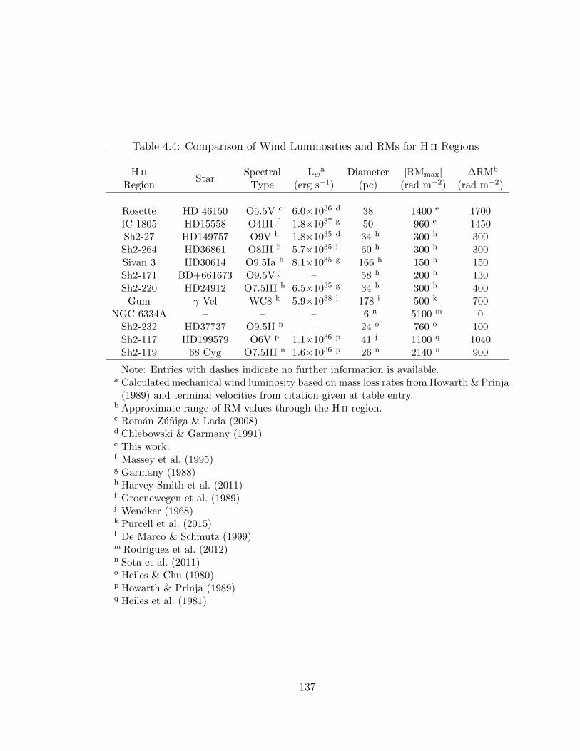
Table 4.4: Comparison of Wind Luminosities and RMs for H ii Regions

H iiStar

Spectral Lwa Diameter |RMmax| ∆RMb

Region Type (erg s−1) (pc) (rad m−2) (rad m−2)

Rosette HD 46150 O5.5V c 6.0×1036 d 38 1400 e 1700IC 1805 HD15558 O4III f 1.8×1037 g 50 960 e 1450Sh2-27 HD149757 O9V h 1.8×1035 d 34 h 300 h 300Sh2-264 HD36861 O8III h 5.7×1035 i 60 h 300 h 300Sivan 3 HD30614 O9.5Ia h 8.1×1035 g 166 h 150 h 150Sh2-171 BD+661673 O9.5V j – 58 h 200 h 130Sh2-220 HD24912 O7.5III h 6.5×1035 g 34 h 300 h 400

Gum γ Vel WC8 k 5.9×1038 l 178 i 500 k 700NGC 6334A – – – 6 n 5100 m 0

Sh2-232 HD37737 O9.5II n – 24 o 760 o 100Sh2-117 HD199579 O6V p 1.1×1036 p 41 j 1100 q 1040Sh2-119 68 Cyg O7.5III n 1.6×1036 p 26 n 2140 n 900

Note: Entries with dashes indicate no further information is available.a Calculated mechanical wind luminosity based on mass loss rates from Howarth & Prinja

(1989) and terminal velocities from citation given at table entry.b Approximate range of RM values through the H ii region.c Roman-Zuniga & Lada (2008)d Chlebowski & Garmany (1991)e This work.f Massey et al. (1995)g Garmany (1988)h Harvey-Smith et al. (2011)i Groenewegen et al. (1989)j Wendker (1968)k Purcell et al. (2015)l De Marco & Schmutz (1999)m Rodrıguez et al. (2012)n Sota et al. (2011)o Heiles & Chu (1980)p Howarth & Prinja (1989)q Heiles et al. (1981)

137

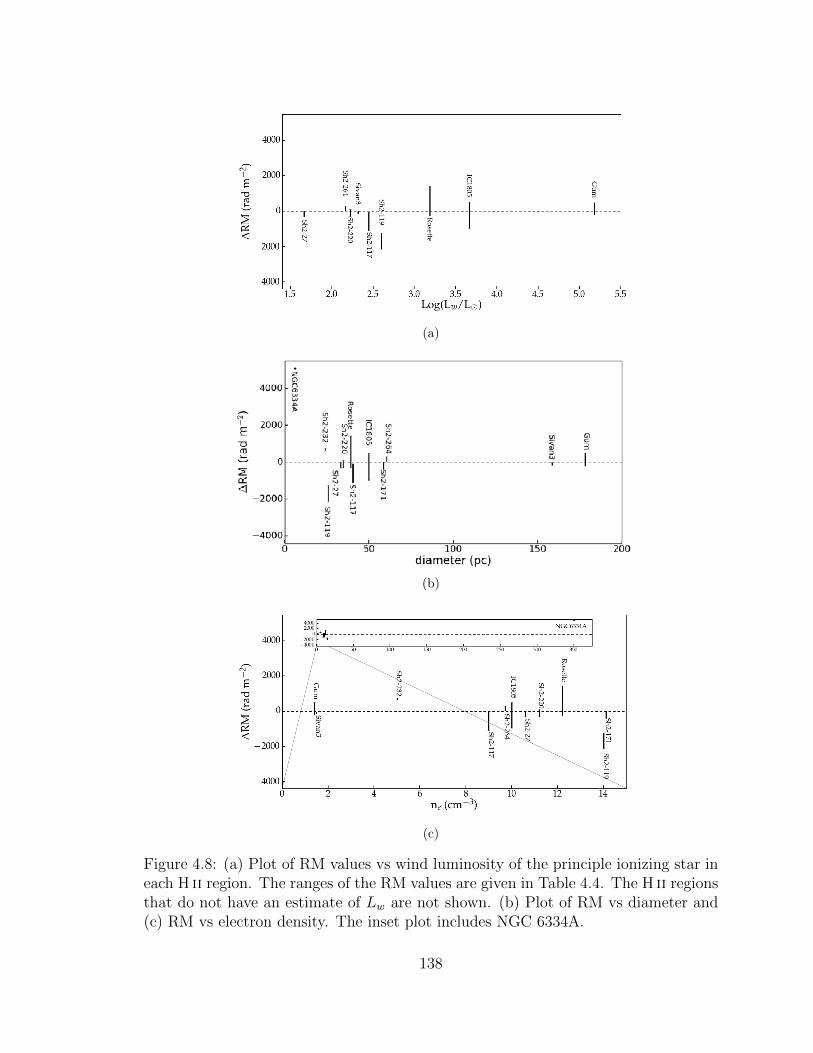
(a)

(b)

(c)

Figure 4.8: (a) Plot of RM values vs wind luminosity of the principle ionizing star ineach H ii region. The ranges of the RM values are given in Table 4.4. The H ii regionsthat do not have an estimate of Lw are not shown. (b) Plot of RM vs diameter and(c) RM vs electron density. The inset plot includes NGC 6334A.

138

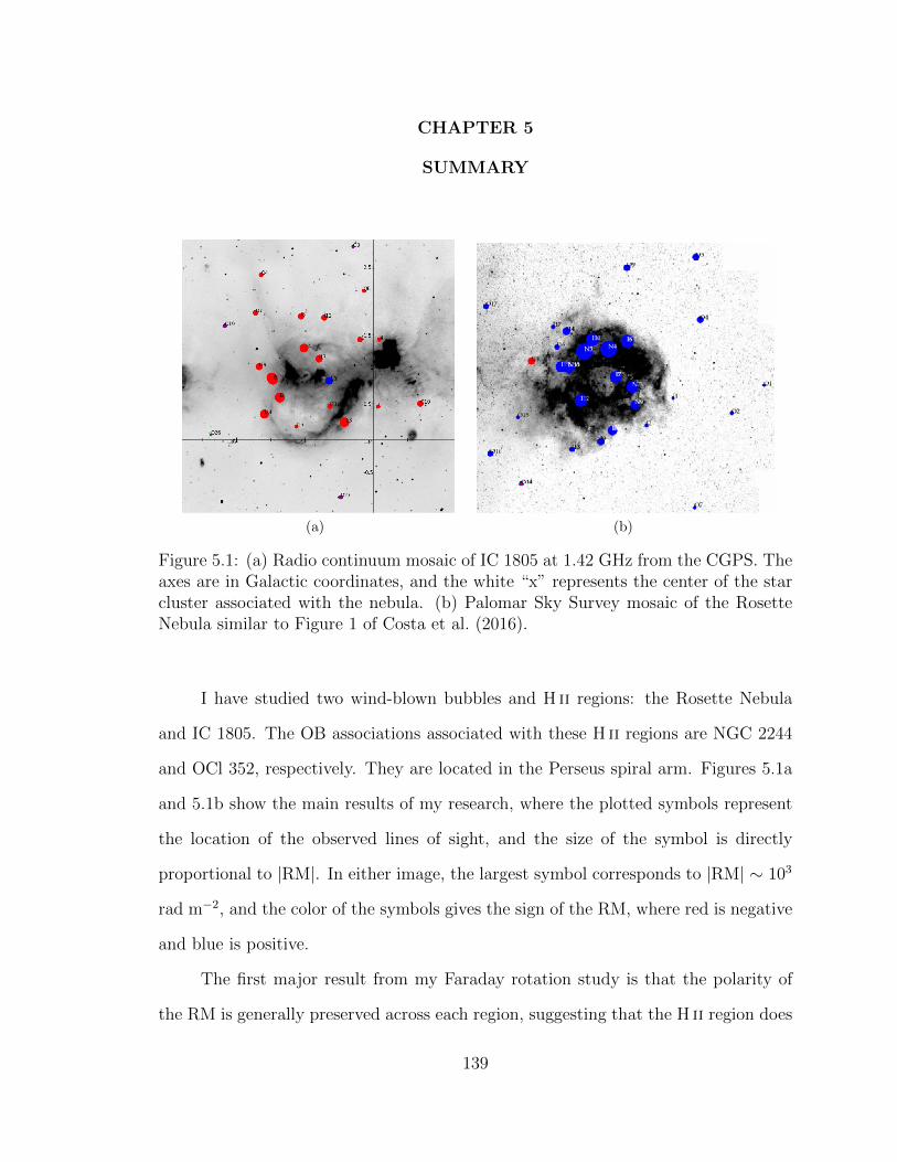
CHAPTER 5

SUMMARY

(a) (b)

Figure 5.1: (a) Radio continuum mosaic of IC 1805 at 1.42 GHz from the CGPS. Theaxes are in Galactic coordinates, and the white “x” represents the center of the starcluster associated with the nebula. (b) Palomar Sky Survey mosaic of the RosetteNebula similar to Figure 1 of Costa et al. (2016).

I have studied two wind-blown bubbles and H ii regions: the Rosette Nebula

and IC 1805. The OB associations associated with these H ii regions are NGC 2244

and OCl 352, respectively. They are located in the Perseus spiral arm. Figures 5.1a

and 5.1b show the main results of my research, where the plotted symbols represent

the location of the observed lines of sight, and the size of the symbol is directly

proportional to |RM|. In either image, the largest symbol corresponds to |RM| ∼ 103

rad m−2, and the color of the symbols gives the sign of the RM, where red is negative

and blue is positive.

The first major result from my Faraday rotation study is that the polarity of

the RM is generally preserved across each region, suggesting that the H ii region does

139

not change the polarity of the parallel component of the magnetic field, BLOS. For

the Rosette (` = 206), I find that BLOS is positive (pointed towards the observer)

(Savage et al., 2013; Costa et al., 2016), and for IC 1805 (` = 135), BLOS is negative

(pointed away). The change in sign of the RM is consistent with a Galactic magnetic

field that follows the Perseus spiral arm in a clockwise fashion (Van Eck et al., 2011).

My results show that the expected polarity of the large-scale Galactic magnetic field

is preserved over large distances (> 3 kpc) in the Perseus arm, and the presence of

the H ii region does not induce a sign change in BLOS within the shell or across the

H ii region.

The second result is that the observed RMs due to the nebulae are similar in

magnitude. The simple shell model described in Savage et al. (2013) predicts RMs

for lines of sight through IC 1805 of 2 – 5 × 103 rad m−2, and from simulations of

wind-blown bubbles, Stil et al. (2009) predict similar magnitudes of the RM. Despite

OCl 352 having higher wind luminosities than NGC 2244, the range of RM values

across the nebulae do not differ dramatically. However, the location of the lines of

sight with the largest values of the RM in each nebula is different. For the Rosette, I

find that the lines of sight through the ionized shell of the H ii region have the largest

RM values. In Section 4.3, I present WISE data for the Rosette, which show that the

lines of sight with the largest values of the RM are not in a PDR around the Rosette;

however for IC 1805, some of the largest RM values are associated with lines of sight

outside the ionized shell, potentially in the PDR.

It seems that the Galactic magnetic field is insensitive to the presence of H ii

regions and stellar bubbles, but H ii regions may not be insensitive to the magnetic

field. The orientation and magnitude of BLOS is not modified inside the shells of

the H ii regions, but theory and simulations suggest that the morphology of the H ii

region and stellar bubble is affected by magnetic fields (Ferriere et al., 1991; Stil et al.,

2009). To further understand the relationship between H ii regions and the Galactic

140

magnetic field, a larger sample of H ii regions is needed.

141

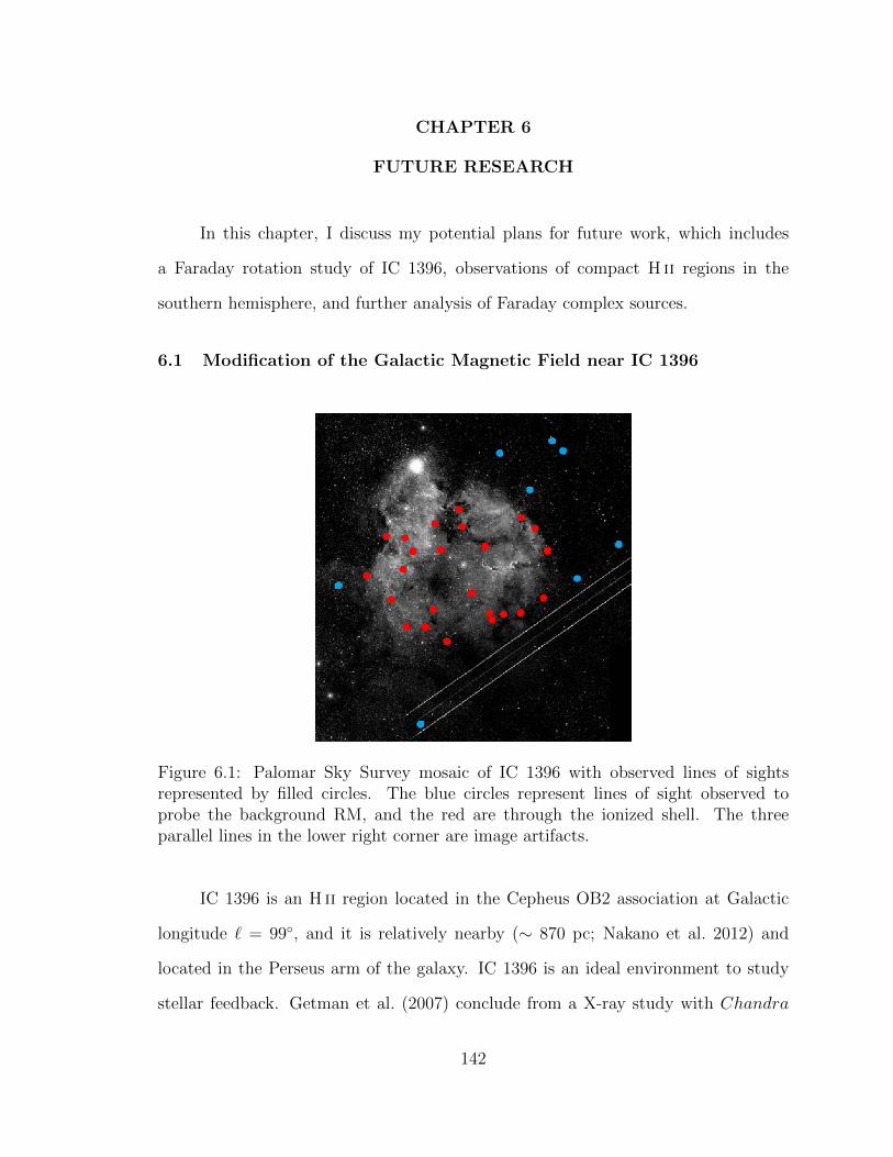
CHAPTER 6

FUTURE RESEARCH

In this chapter, I discuss my potential plans for future work, which includes

a Faraday rotation study of IC 1396, observations of compact H ii regions in the

southern hemisphere, and further analysis of Faraday complex sources.

6.1 Modification of the Galactic Magnetic Field near IC 1396

Figure 6.1: Palomar Sky Survey mosaic of IC 1396 with observed lines of sightsrepresented by filled circles. The blue circles represent lines of sight observed toprobe the background RM, and the red are through the ionized shell. The threeparallel lines in the lower right corner are image artifacts.

IC 1396 is an H ii region located in the Cepheus OB2 association at Galactic

longitude ` = 99, and it is relatively nearby (∼ 870 pc; Nakano et al. 2012) and

located in the Perseus arm of the galaxy. IC 1396 is an ideal environment to study

stellar feedback. Getman et al. (2007) conclude from a X-ray study with Chandra

142

that IC 1396 is a region with triggered star formation that is the result of a radiation-

driven implosion (RDI), which has a characteristic direction oriented age gradient such

that older stars are closer to the ionizing star. In their study of pre-main sequence

stars, Nakano et al. (2012) also see evidence of triggered star formation as a result

of the expansion of the H ii region. To probe properties of the magnetic field in the

shell of the H ii region and stellar bubble, I have completed observations of 32 lines

of sight through or near to the shell of the H ii region, shown in Figure 6.1.

6.2 Compact H ii Regions at ` ∼ 328

An Evolutionary Map of the Universe (EMU) early science project is to study

discrete Galactic radio sources at ` ∼ 328. In late 2017, I and Dr. S. Brown proposed

a POSSUM early science project with ASKAP for polarimetric observations in this

field to probe the plasma structure of compact H ii regions. The observations will

most likely be complete in 2018. In addition to studying the RM structure through

compact H ii regions, this project will test analysis techniques and the POSSUM data

reduction pipeline.

6.3 Faraday complex Sources Using Simulated Data

I intend to continue my analysis of Faraday complex sources. I will simulate

Faraday complex spectra to compare the preferred depolarization model when the

choice of channel width (e.g., 128 MHz vs 4 MHz) in Q and U is varied and when

the use of fractional vs corrected Q and U spectra is used (see Section 4.2). I already

have the Python code that will create the simulated spectra, and I can continue to

explore the QU analysis technique.

143

APPENDIX A

CASA MAPS FOR LINES OF SIGHT THROUGH OR NEAR TO IC

1805

In this appendix, I present radio maps for the sources with lines of sight through

IC 1805. In each map, the gray scale is the linear polarized intensity, the line segments

are the polarization position angle, and the contours are Stokes I at –2, –1, 2, 10, 20,

40, 60, and 80% of the peak intensity of the source.

144

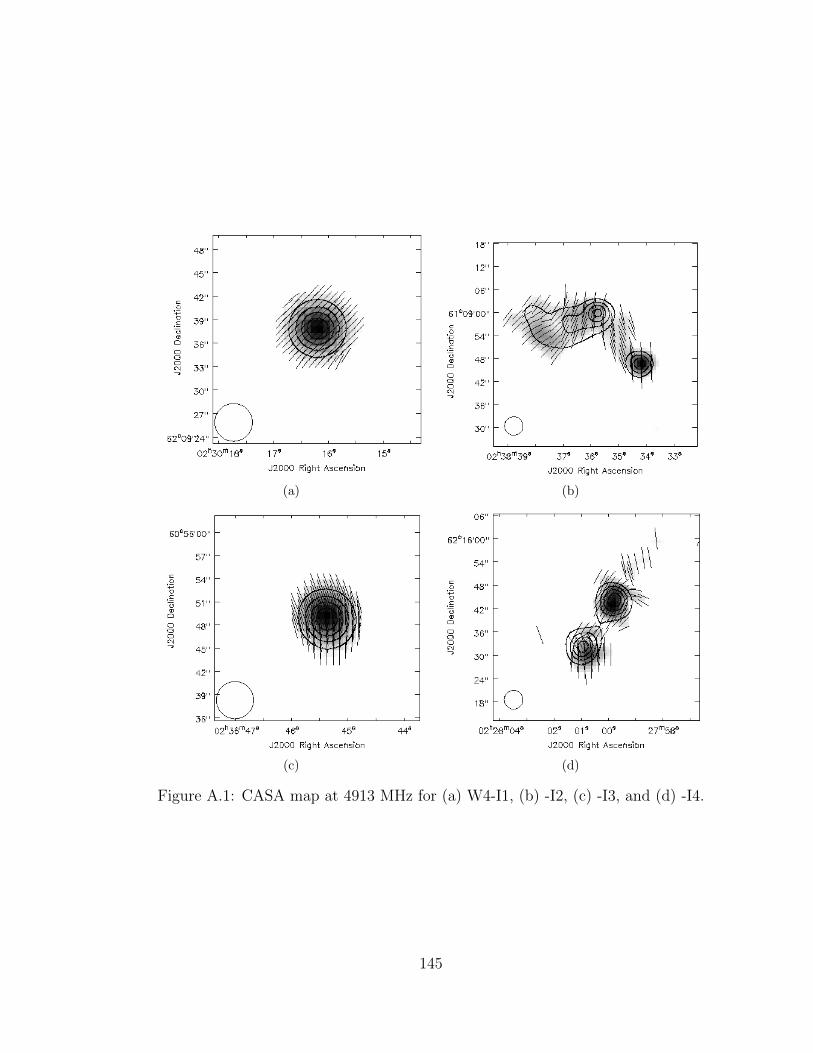
(a) (b)

(c) (d)

Figure A.1: CASA map at 4913 MHz for (a) W4-I1, (b) -I2, (c) -I3, and (d) -I4.

145

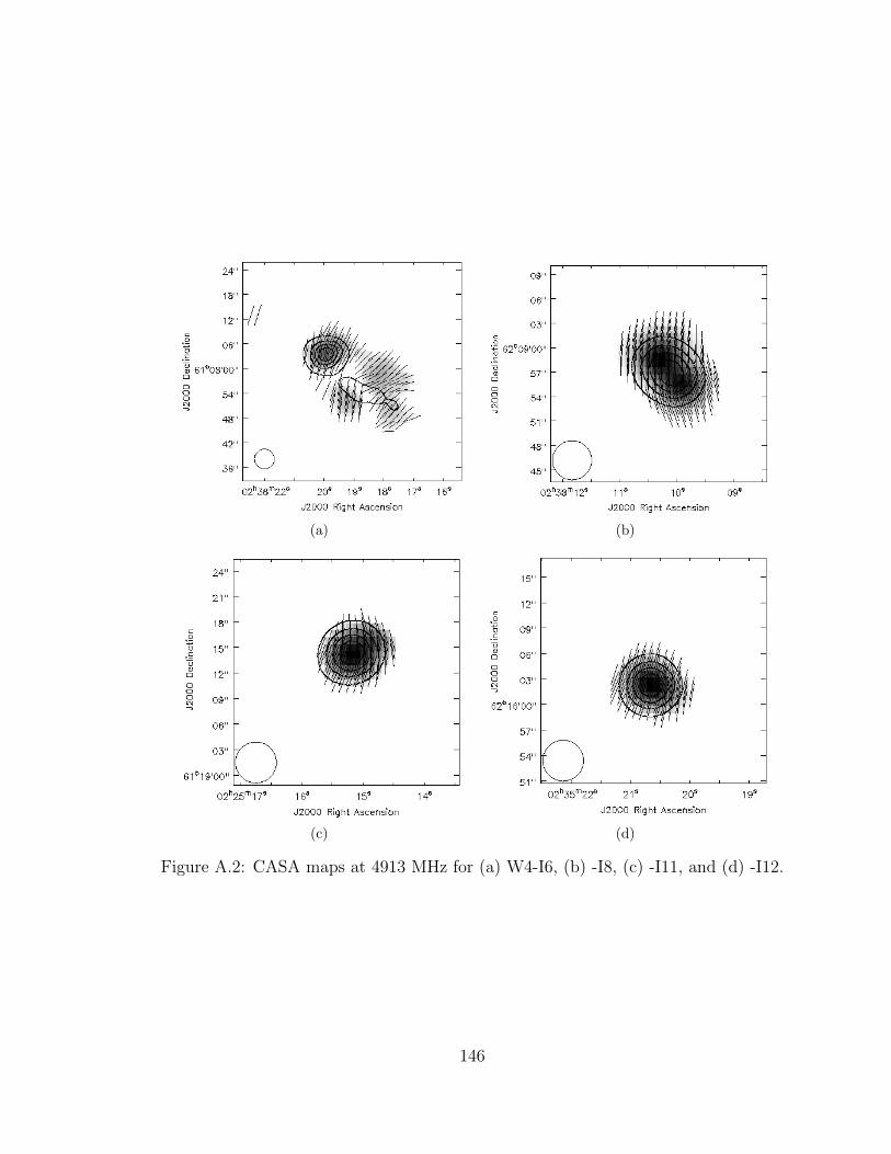
(a) (b)

(c) (d)

Figure A.2: CASA maps at 4913 MHz for (a) W4-I6, (b) -I8, (c) -I11, and (d) -I12.

146

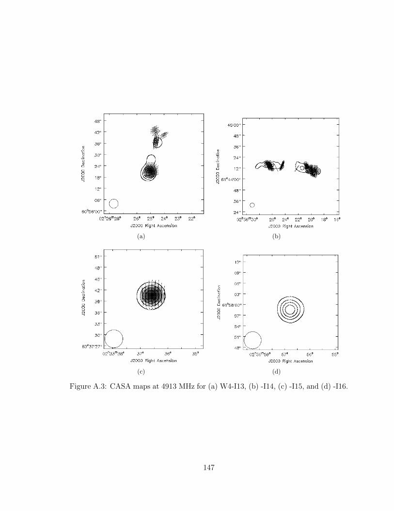
(a) (b)

(c) (d)

Figure A.3: CASA maps at 4913 MHz for (a) W4-I13, (b) -I14, (c) -I15, and (d) -I16.

147

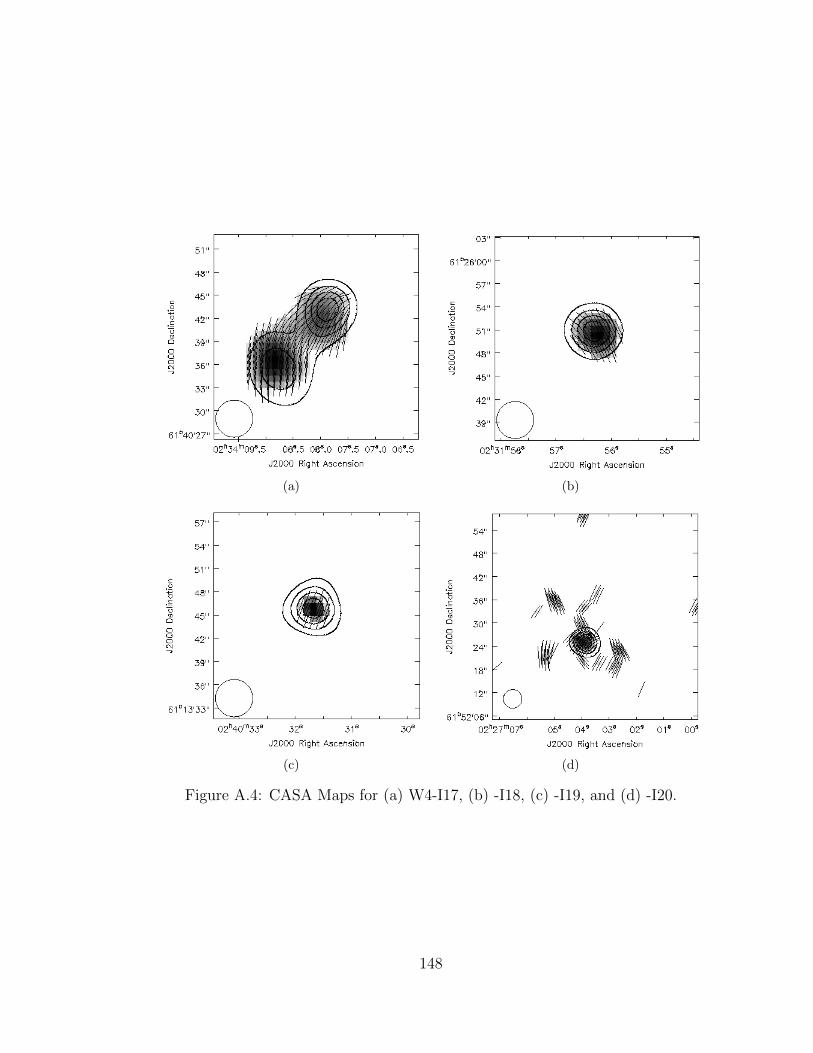
(a) (b)

(c) (d)

Figure A.4: CASA Maps for (a) W4-I17, (b) -I18, (c) -I19, and (d) -I20.

148

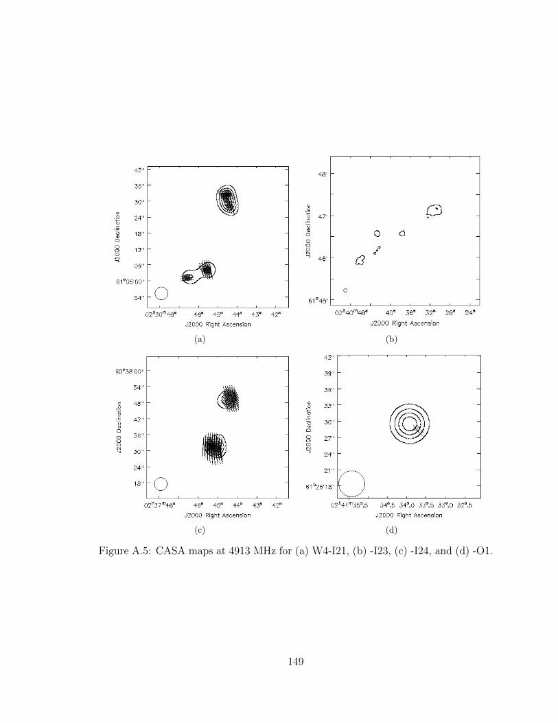
(a) (b)

(c) (d)

Figure A.5: CASA maps at 4913 MHz for (a) W4-I21, (b) -I23, (c) -I24, and (d) -O1.

149

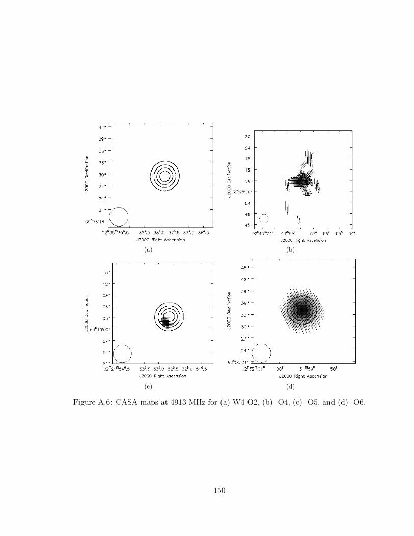
(a) (b)

(c) (d)

Figure A.6: CASA maps at 4913 MHz for (a) W4-O2, (b) -O4, (c) -O5, and (d) -O6.

150

(a) (b)

(c)

Figure A.7: CASA maps at 4913 MHz for (a) W4-O7, (b) -O8, and (c) -O10.

151

APPENDIX B

FIGURES FOR RM SYNTHESIS ANALYSIS

The figures presented in this Appendix are plots of F (φ) for lines of sight through

IC 1805 and the Rosette Nebula. In each image, the amplitude of F (φ) (P ) is the solid

curve, the real part of F (φ) (Q) is the dashed curve, and the imaginary part of F (φ)

(U) is the dotted curve. The clean components from rmclean are also represented

by the vertical lines. The amplitude is shown in red, the real part is blue, and the

imaginary part is green. If no clean components are shown, it indicates that there

was not a significant (> 7σQU) peak in F (φ). The range in φ has been reduced to

show the maximum amount of structure. No other peaks in F (φ) are seen out to ±

10,000 rad m−2. The RMSF is presented in Figures 3.7b and 2.6 for IC 1805 and the

Rosette lines of sight, respectively.

152

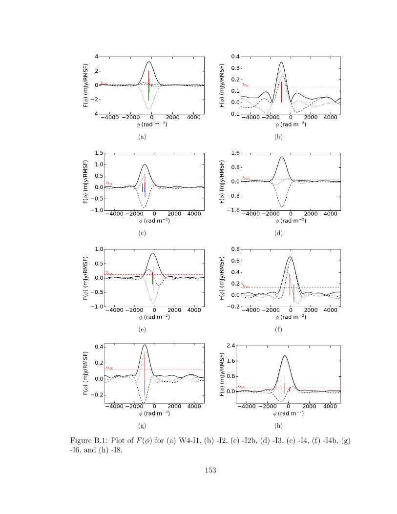
(a) (b)

(c) (d)

(e) (f)

(g) (h)

Figure B.1: Plot of F (φ) for (a) W4-I1, (b) -I2, (c) -I2b, (d) -I3, (e) -I4, (f) -I4b, (g)-I6, and (h) -I8.

153

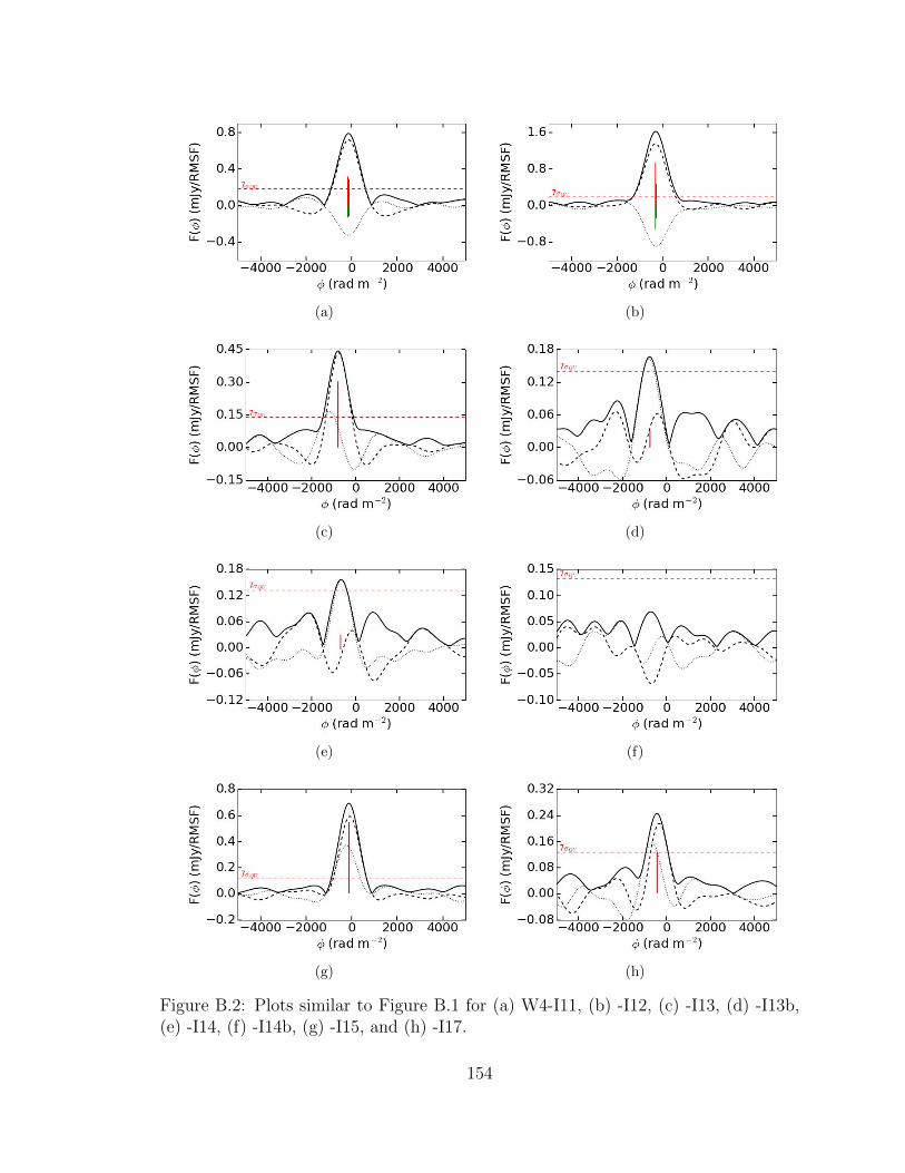
(a) (b)

(c) (d)

(e) (f)

(g) (h)

Figure B.2: Plots similar to Figure B.1 for (a) W4-I11, (b) -I12, (c) -I13, (d) -I13b,(e) -I14, (f) -I14b, (g) -I15, and (h) -I17.

154

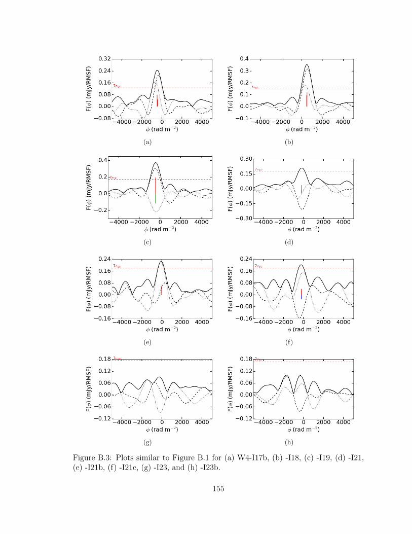
(a) (b)

(c) (d)

(e) (f)

(g) (h)

Figure B.3: Plots similar to Figure B.1 for (a) W4-I17b, (b) -I18, (c) -I19, (d) -I21,(e) -I21b, (f) -I21c, (g) -I23, and (h) -I23b.

155

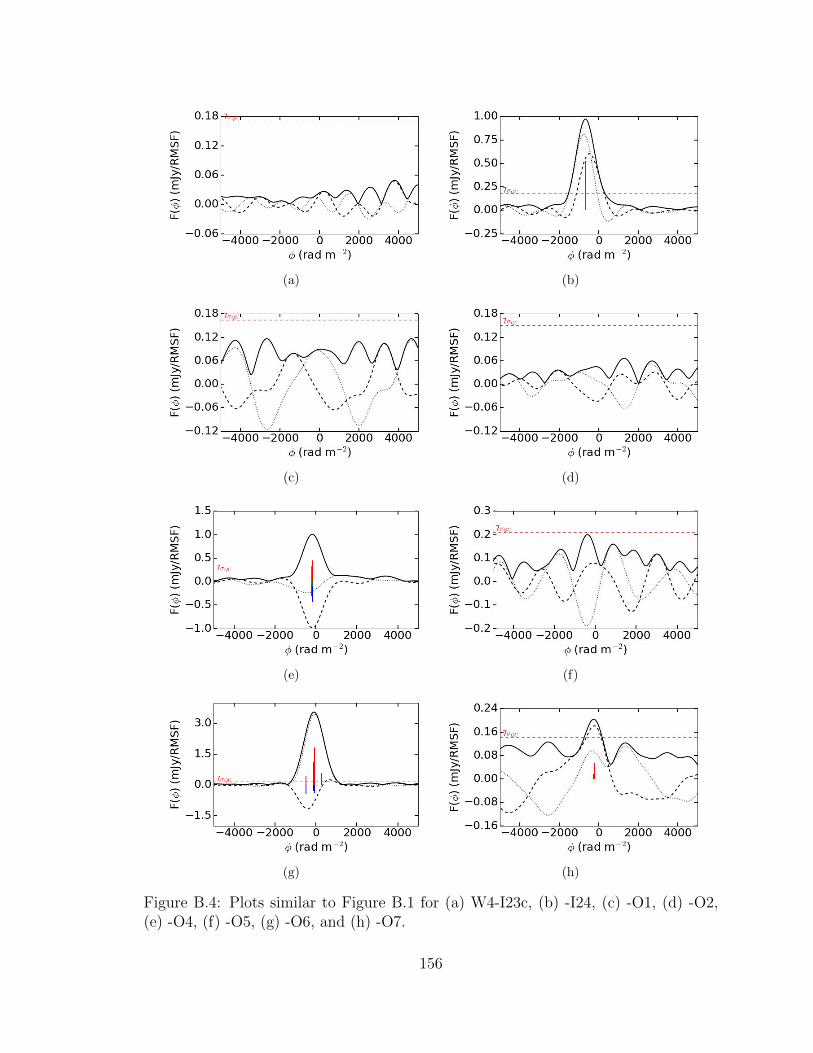
(a) (b)

(c) (d)

(e) (f)

(g) (h)

Figure B.4: Plots similar to Figure B.1 for (a) W4-I23c, (b) -I24, (c) -O1, (d) -O2,(e) -O4, (f) -O5, (g) -O6, and (h) -O7.

156

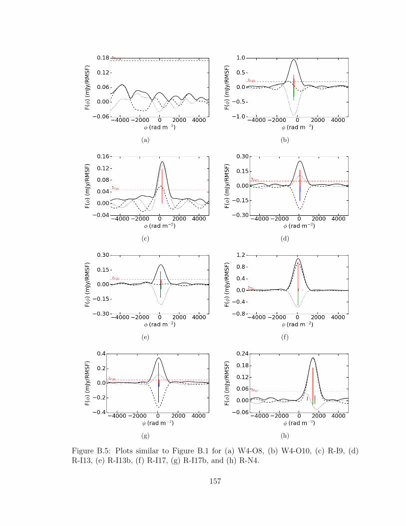
(a) (b)

(c) (d)

(e) (f)

(g) (h)

Figure B.5: Plots similar to Figure B.1 for (a) W4-O8, (b) W4-O10, (c) R-I9, (d)R-I13, (e) R-I13b, (f) R-I17, (g) R-I17b, and (h) R-N4.

157

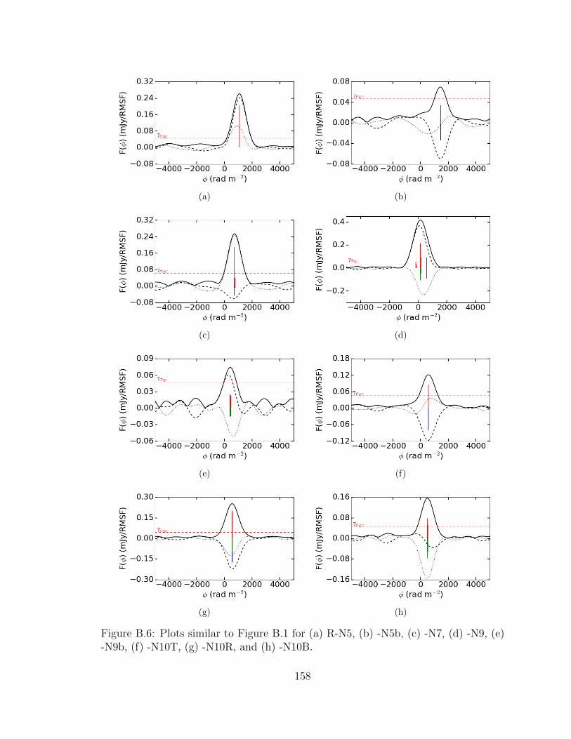
(a) (b)

(c) (d)

(e) (f)

(g) (h)

Figure B.6: Plots similar to Figure B.1 for (a) R-N5, (b) -N5b, (c) -N7, (d) -N9, (e)-N9b, (f) -N10T, (g) -N10R, and (h) -N10B.

158

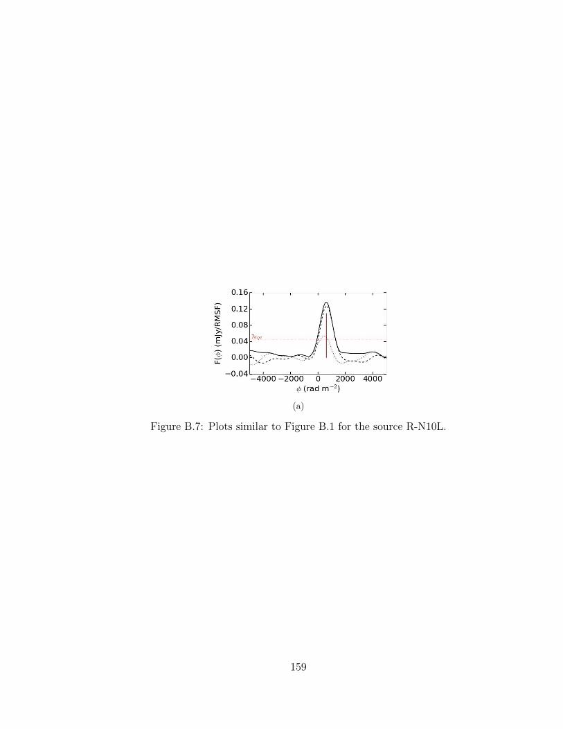
(a)

Figure B.7: Plots similar to Figure B.1 for the source R-N10L.

159

APPENDIX C

FIGURES AND TABLES FOR QU ANALYSIS

The tables and figures below are discussed in Chapter 4, Section 4.2.3.

160

Tab

leC

.1:

Res

ult

sof

QU

Anal

ysi

sfo

r4

MH

z“F

ract

ional

”D

ata

Sou

rce

Mod

elp

0χ

0φ

0p

1χ

1φ

1σ

RM

χ2 u

BIC

AIC

(mJy)

(o)

(rad

m2)

(mJy)

(o)

(rad

m2)

(rad

m2)

W4-

I1E

FD

6217

4-2

72—

——

142

2.1

5-2

149

-2165

Un

ifor

mS

lab

6417

0-4

86—

——

—2.7

0-1

964

-1975

Un

ifor

mS

lab

+F

arad

ayT

hin

21.0

0.0

177

4816

2-2

65

—1.9

7-2

214

-2238

W4-

I3F

arad

ayT

hin

2022

-861

——

——

2.2

8-1

800

-1811

EF

D24

23-8

62—

——

80

2.2

1-1

818

-1833

Un

ifor

mS

lab

+F

arad

ayT

hin

270.

012

021

23-8

63

—2.1

7-1

825

-1848

W4-

I8F

arad

ayT

hin

6065

-305

——

——

2.4

3-7

92

-803

EF

D61

65-3

05—

——

8.0

2.4

5-7

87

-801

Un

ifor

mS

lab

7641

-359

——

——

3.7

2-4

65

-475

W4-

I12

Far

aday

Th

in21

37-3

04—

——

—2.1

4-1

453

-1463

EF

D21

37-3

04—

——

8.4

2.1

5-1

447

-1461

Un

ifor

mS

lab

2519

-391

——

——

3.6

2-1

075

-1086

Col

um

ns

one

and

two

give

the

sou

rce

and

the

RM

der

ived

from

RM

Synth

esis

.C

olu

mn

thre

egiv

esth

eco

mp

on

ents

of

the

mod

el.

Wh

enth

eor

der

ofm

ult

iple

com

pon

ents

isim

por

tant,

the

firs

tco

mp

onen

tco

rres

pon

ds

tosu

bsc

rip

t‘0

’.C

olu

mn

sfo

ur

tote

ngi

veth

ep

aram

eter

sfo

rth

ed

epol

ariz

atio

nm

od

el.

Col

um

nel

even

list

sth

ere

du

cedχ

2,

colu

mn

twel

vegiv

esth

eB

IC,

and

colu

mn

thir

teen

give

sth

eA

IC.

161

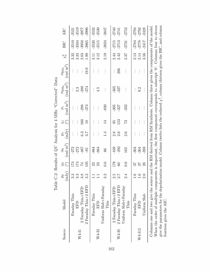
Tab

leC

.2:

Res

ult

sof

QU

Anal

ysi

sfo

r4

MH

z“C

orre

cted

”D

ata

Sou

rce

Mod

elp

0χ

0φ

0p

1χ

1φ

1σ

RM

0σ

RM

1χ

2 uB

ICA

IC(m

Jy)

(o)

(rad

m2)

(mJy)

(o)

(rad

m2)

(rad

m2)

(rad

m2)

W4-

I1

Far

aday

Th

in3.

317

4-2

72—

——

——

3.3

2-3

510

-3521

EF

D3.

317

4-2

72—

——

2.3

—3.3

3-3

504

-3519

2F

arad

ayT

hin

+E

FD

3.8

74-4

676.

316

0-2

88-2

88

—2.0

3-3

950

-3977

2F

arad

ayT

hin

+2

EF

D3.

210

5-8

53.

718

-374

-374

19.9

1.9

9-3

965

-3996

W4-

I3F

arad

ayT

hin

1.1

23-8

64—

——

——

3.1

1-3

520

-3532

EF

D1.

123

-864

——

—4.5

—3.1

2-3

515

-3530

Un

ifor

mS

lab

+F

arad

ayT

hin

3.2

0.0

661.

414

-830

——

2.1

9-3

824

-3847

W4-

I82

Far

aday

Th

in+

EF

D2.

517

8-1

692.

895

-305

-305

—2.4

4-2

715

-2740

2F

arad

ayT

hin

+2

EF

D2.

760

–292

2.6

153

-327

-327

206

2.4

2-2

713

-2741

Un

ifor

mS

lab

+F

arad

ayT

hin

2.4

0.0

163

2.6

73-3

32—

—2.3

7-2

731

-2752

W4-

I12

Far

aday

Th

in1.

637

-304

——

——

—2.1

3-2

784

-2794

EF

D1.

637

-304

——

—9.2

—2.1

4-2

778

-2792

Un

ifor

mS

lab

2.0

20-3

93—

——

——

3.5

6-2

417

-2428

Col

um

ns

one

and

two

give

the

sou

rce

and

the

RM

der

ived

from

RM

Synth

esis

.C

olu

mn

thre

egiv

esth

eco

mp

onen

tsof

the

model

.W

hen

the

ord

erof

mu

ltip

leco

mp

onen

tsis

imp

orta

nt,

the

firs

tco

mp

onen

tco

rres

pon

ds

tosu

bsc

rip

t‘0

’.C

olu

mn

sfo

ur

toel

even

give

the

par

amet

ers

for

the

dep

olar

izati

onm

od

el.

Col

um

ntw

elve

list

sth

ere

du

cedχ

2,

colu

mn

thir

teen

giv

esth

eB

IC,

an

dco

lum

nfo

urt

een

give

sth

eA

IC.

162

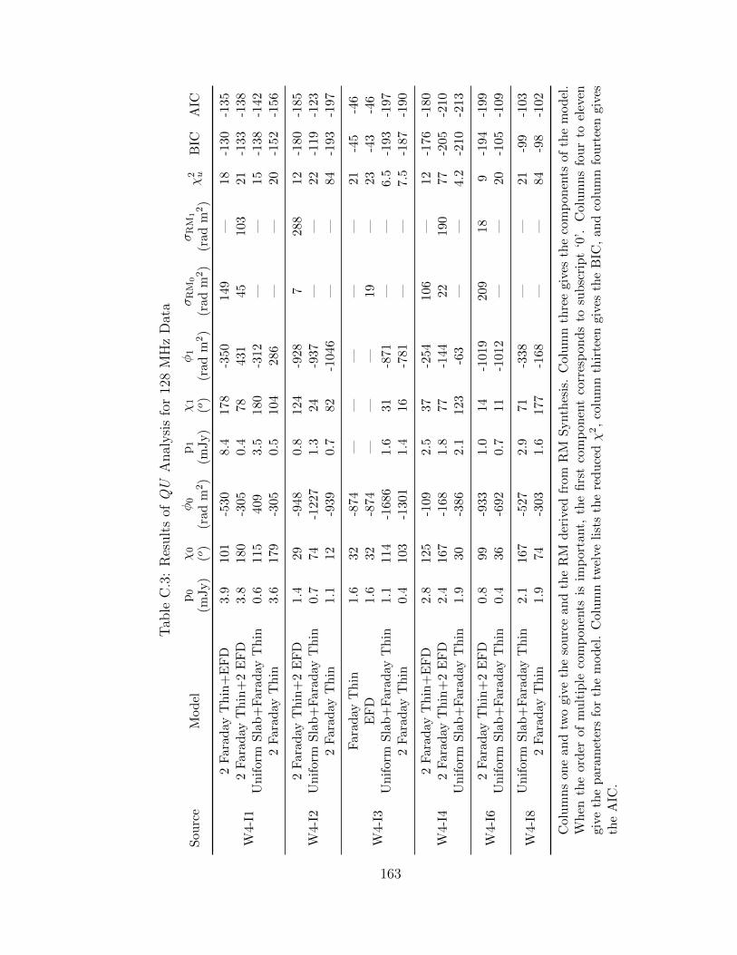
Tab

leC

.3:

Res

ult

sof

QU

Anal

ysi

sfo

r12

8M

Hz

Dat

a

Sou

rce

Mod

elp

0χ

0φ

0p

1χ

1φ

1σ

RM

0σ

RM

1χ

2 uB

ICA

IC(m

Jy)

(o)

(rad

m2)

(mJy)

(o)

(rad

m2)

(rad

m2)

(rad

m2)

W4-

I1

2F

arad

ayT

hin

+E

FD

3.9

101

-530

8.4

178

-350

149

—18

-130

-135

2F

arad

ayT

hin

+2

EF

D3.

818

0-3

050.

478

431

45

103

21

-133

-138

Un

ifor

mS

lab

+F

arad

ayT

hin

0.6

115

409

3.5

180

-312

——

15

-138

-142

2F

arad

ayT

hin

3.6

179

-305

0.5

104

286

——

20

-152

-156

W4-

I22

Far

aday

Th

in+

2E

FD

1.4

29-9

480.

812

4-9

287

288

12

-180

-185

Un

ifor

mS

lab

+F

arad

ayT

hin

0.7

74-1

227

1.3

24-9

37—

—22

-119

-123

2F

arad

ayT

hin

1.1

12-9

390.

782

-104

6—

—84

-193

-197

W4-

I3

Far

aday

Th

in1.

632

-874

——

——

—21

-45

-46

EF

D1.

632

-874

——

—19

—23

-43

-46

Un

ifor

mS

lab

+F

arad

ayT

hin

1.1

114

-168

61.

631

-871

——

6.5

-193

-197

2F

arad

ayT

hin

0.4

103

-130

11.

416

-781

——

7.5

-187

-190

W4-

I42

Far

aday

Th

in+

EF

D2.

812

5-1

092.

537

-254

106

—12

-176

-180

2F

arad

ayT

hin

+2

EF

D2.

416

7-1

681.

877

-144

22

190

77

-205

-210

Un

ifor

mS

lab

+F

arad

ayT

hin

1.9

30-3

862.

112

3-6

3—

—4.2

-210

-213

W4-

I62

Far

aday

Th

in+

2E

FD

0.8

99-9

331.

014

-101

9209

18

9-1

94

-199

Un

ifor

mS

lab

+F

arad

ayT

hin

0.4

36-6

920.

711

-101

2—

—20

-105

-109

W4-

I8U

nif

orm

Sla

b+

Far

aday

Th

in2.

116

7-5

272.

971

-338

——

21

-99

-103

2F

arad

ayT

hin

1.9

74-3

031.

617

7-1

68—

—84

-98

-102

Col

um

ns

one

and

two

give

the

sou

rce

and

the

RM

der

ived

from

RM

Synth

esis

.C

olu

mn

thre

egiv

esth

eco

mp

on

ents

of

the

model

.W

hen

the

ord

erof

mu

ltip

leco

mp

onen

tsis

imp

orta

nt,

the

firs

tco

mp

onen

tco

rres

pon

ds

tosu

bsc

rip

t‘0

’.C

olu

mn

sfo

ur

toel

even

give

the

par

amet

ers

for

the

mod

el.

Col

um

ntw

elve

list

sth

ere

du

cedχ

2,

colu

mn

thir

teen

giv

esth

eB

IC,

an

dco

lum

nfo

urt

een

giv

esth

eA

IC.

163

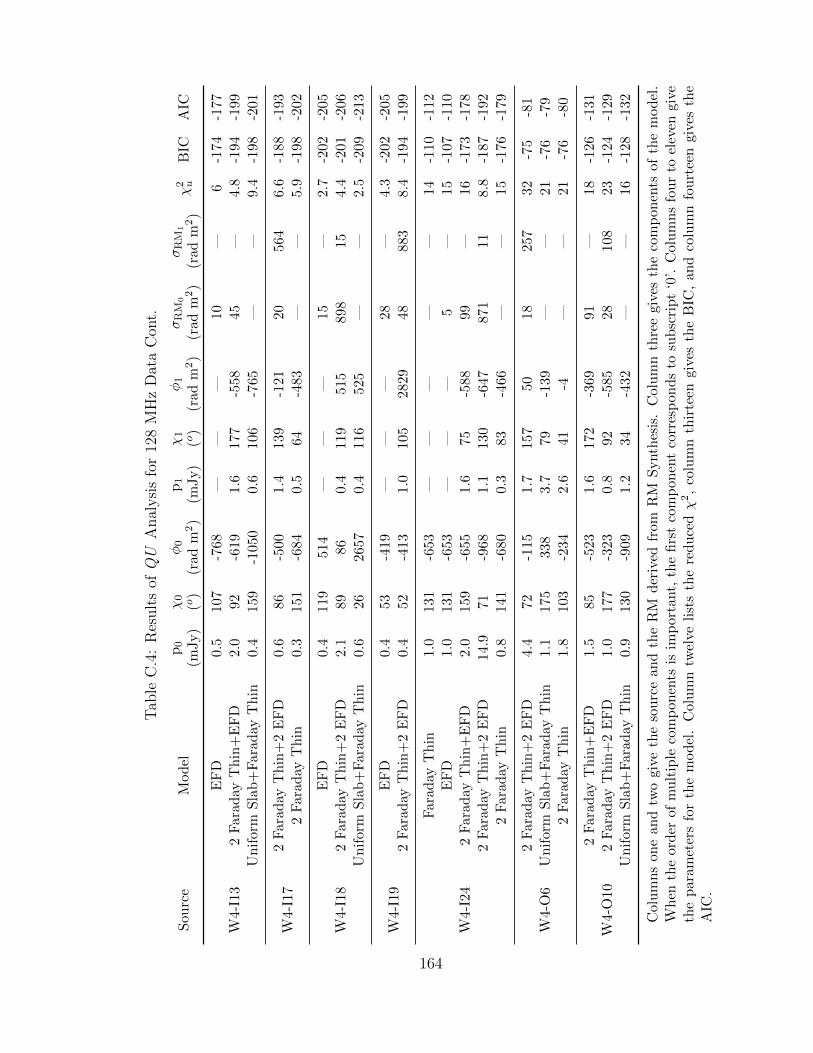
Tab

leC

.4:

Res

ult

sof

QU

Anal

ysi

sfo

r12

8M

Hz

Dat

aC

ont.

Sou

rce

Mod

elp

0χ

0φ

0p

1χ

1φ

1σ

RM

0σ

RM

1χ

2 uB

ICA

IC(m

Jy)

(o)

(rad

m2)

(mJy)

(o)

(rad

m2)

(rad

m2)

(rad

m2)

W4-

I13

EF

D0.

510

7-7

68—

——

10

—6

-174

-177

2F

arad

ayT

hin

+E

FD

2.0

92-6

191.

617

7-5

5845

—4.8

-194

-199

Un

ifor

mS

lab

+F

arad

ayT

hin

0.4

159

-105

00.

610

6-7

65—

—9.4

-198

-201

W4-

I17

2F

arad

ayT

hin

+2

EF

D0.

686

-500

1.4

139

-121

20

564

6.6

-188

-193

2F

arad

ayT

hin

0.3

151

-684

0.5

64-4

83—

—5.9

-198

-202

W4-

I18

EF

D0.

411

951

4—

——

15

—2.7

-202

-205

2F

arad

ayT

hin

+2

EF

D2.

189

860.

411

951

5898

15

4.4

-201

-206

Un

ifor

mS

lab

+F

arad

ayT

hin

0.6

2626

570.

411

652

5—

—2.5

-209

-213

W4-

I19

EF

D0.

453

-419

——

—28

—4.3

-202

-205

2F

arad

ayT

hin

+2

EF

D0.

452

-413

1.0

105

2829

48

883

8.4

-194

-199

W4-

I24

Far

aday

Th

in1.

013

1-6

53—

——

——

14

-110

-112

EF

D1.

013

1-6

53—

——

5—

15

-107

-110

2F

arad

ayT

hin

+E

FD

2.0

159

-655

1.6

75-5

8899

—16

-173

-178

2F

arad

ayT

hin

+2

EF

D14

.971

-968

1.1

130

-647

871

11

8.8

-187

-192

2F

arad

ayT

hin

0.8

141

-680

0.3

83-4

66—

—15

-176

-179

W4-

O6

2F

arad

ayT

hin

+2

EF

D4.

472

-115

1.7

157

5018

257

32

-75

-81

Un

ifor

mS

lab

+F

arad

ayT

hin

1.1

175

338

3.7

79-1

39—

—21

-76

-79

2F

arad

ayT

hin

1.8

103

-234

2.6

41-4

——

21

-76

-80

W4-

O10

2F

arad

ayT

hin

+E

FD

1.5

85-5

231.

617

2-3

6991

—18

-126

-131

2F

arad

ayT

hin

+2

EF

D1.

017

7-3

230.

892

-585

28

108

23

-124

-129

Un

ifor

mS

lab

+F

arad

ayT

hin

0.9

130

-909

1.2

34-4

32—

—16

-128

-132

Col

um

ns

one

and

two

give

the

sou

rce

and

the

RM

der

ived

from

RM

Synth

esis

.C

olu

mn

thre

egiv

esth

eco

mp

on

ents

of

the

mod

el.

Wh

enth

eor

der

ofm

ult

iple

com

pon

ents

isim

por

tant,

the

firs

tco

mp

onen

tco

rres

pon

ds

tosu

bsc

rip

t‘0

’.C

olu

mn

sfo

ur

toel

even

giv

eth

ep

aram

eter

sfo

rth

em

od

el.

Col

um

ntw

elve

list

sth

ere

du

cedχ

2,

colu

mn

thir

teen

giv

esth

eB

IC,

an

dco

lum

nfo

urt

een

giv

esth

eA

IC.

164

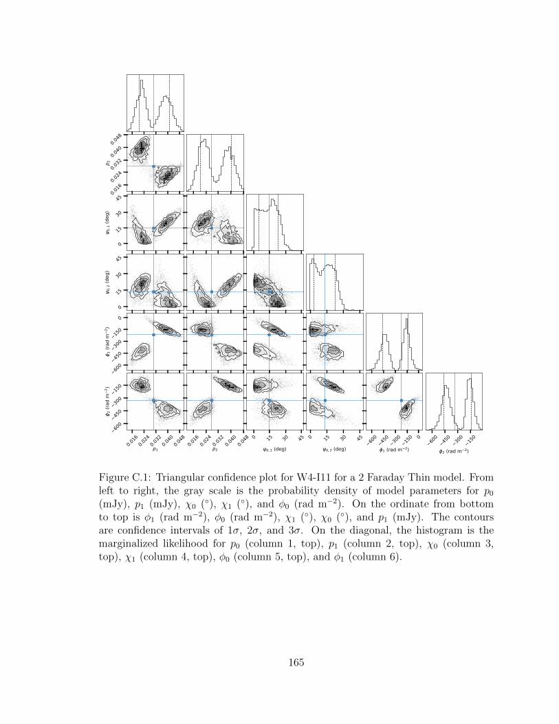
0.016

0.024

0.032

0.040

0.048

p 2

0

15

30

45

0,1 (

deg)

0

15

30

45

0,2 (

deg)

600

450

300

150

0

1 (ra

d m

2 )

0.016

0.024

0.032

0.040

0.048

p1

600

450

300

150

2 (ra

d m

2 )

0.016

0.024

0.032

0.040

0.048

p2

0 15 30 45

0, 1 (deg)

0 15 30 45

0, 2 (deg)60

045

030

015

0 0

1 (rad m 2)60

045

030

015

0

2 (rad m 2)

Figure C.1: Triangular confidence plot for W4-I11 for a 2 Faraday Thin model. Fromleft to right, the gray scale is the probability density of model parameters for p0

(mJy), p1 (mJy), χ0 (), χ1 (), and φ0 (rad m−2). On the ordinate from bottomto top is φ1 (rad m−2), φ0 (rad m−2), χ1 (), χ0 (), and p1 (mJy). The contoursare confidence intervals of 1σ, 2σ, and 3σ. On the diagonal, the histogram is themarginalized likelihood for p0 (column 1, top), p1 (column 2, top), χ0 (column 3,top), χ1 (column 4, top), φ0 (column 5, top), and φ1 (column 6).

165

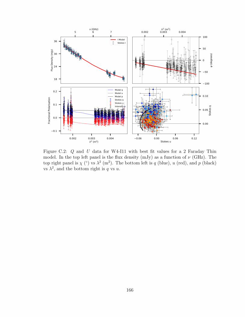
5 6 7 (GHz)

18

24

30

36

Flux

Den

sity

(mJy

)

I ModelStokes I

0.002 0.003 0.0042 (m2)

0.1

0.0

0.1

0.2

Frac

tiona

l Pol

arisa

tion

Model qModel uModel pStokes qStokes uIntensity p

0.002 0.003 0.0042 (m2)

100

50

0

50

100

(deg

rees

)

0.06 0.00 0.06 0.12Stokes u

0.00

0.05

0.10

Stok

es q

Figure C.2: Q and U data for W4-I11 with best fit values for a 2 Faraday Thinmodel. In the top left panel is the flux density (mJy) as a function of ν (GHz). Thetop right panel is χ () vs λ2 (m2). The bottom left is q (blue), u (red), and p (black)vs λ2, and the bottom right is q vs u.

166

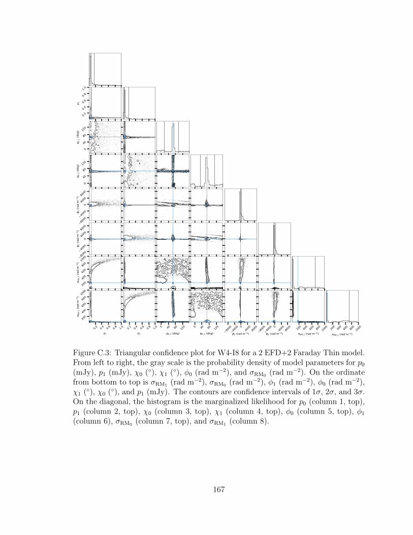
0.20.40.60.81.0

p 2

0

40

8012

0

0,1 (

deg)

0

40

8012

0

0,2 (

deg)

8000

4000

040

0080

00

1 (ra

d m

2 )

8000

4000

040

0080

00

2 (ra

d m

2 )

200

400

600

800

1000

RM,1

(rad

m2 )

0.2 0.4 0.6 0.8 1.0

p1

200

400

600

800

1000

RM,2

(rad

m2 )

0.2 0.4 0.6 0.8 1.0

p2

0 40 80 120

0, 1 (deg)

0 40 80 120

0, 2 (deg)80

0040

00 040

0080

00

1 (rad m 2)80

0040

00 040

0080

00

2 (rad m 2)20

040

060

080

010

00

RM, 1 (rad m 2)20

040

060

080

010

00

RM, 2 (rad m 2)

Figure C.3: Triangular confidence plot for W4-I8 for a 2 EFD+2 Faraday Thin model.From left to right, the gray scale is the probability density of model parameters for p0

(mJy), p1 (mJy), χ0 (), χ1 (), φ0 (rad m−2), and σRM0 (rad m−2). On the ordinatefrom bottom to top is σRM1 (rad m−2), σRM0 (rad m−2), φ1 (rad m−2), φ0 (rad m−2),χ1 (), χ0 (), and p1 (mJy). The contours are confidence intervals of 1σ, 2σ, and 3σ.On the diagonal, the histogram is the marginalized likelihood for p0 (column 1, top),p1 (column 2, top), χ0 (column 3, top), χ1 (column 4, top), φ0 (column 5, top), φ1

(column 6), σRM0 (column 7, top), and σRM1 (column 8).

167

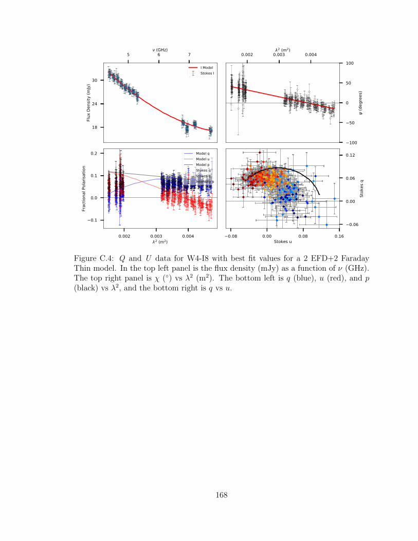
5 6 7 (GHz)

18

24

30Fl

ux D

ensit

y (m

Jy)

I ModelStokes I

0.002 0.003 0.0042 (m2)

0.1

0.0

0.1

0.2

Frac

tiona

l Pol

arisa

tion

Model qModel uModel pStokes qStokes uIntensity p

0.002 0.003 0.0042 (m2)

100

50

0

50

100

(deg

rees

)

0.08 0.00 0.08 0.16Stokes u

0.06

0.00

0.06

0.12

Stok

es q

Figure C.4: Q and U data for W4-I8 with best fit values for a 2 EFD+2 FaradayThin model. In the top left panel is the flux density (mJy) as a function of ν (GHz).The top right panel is χ () vs λ2 (m2). The bottom left is q (blue), u (red), and p(black) vs λ2, and the bottom right is q vs u.

168

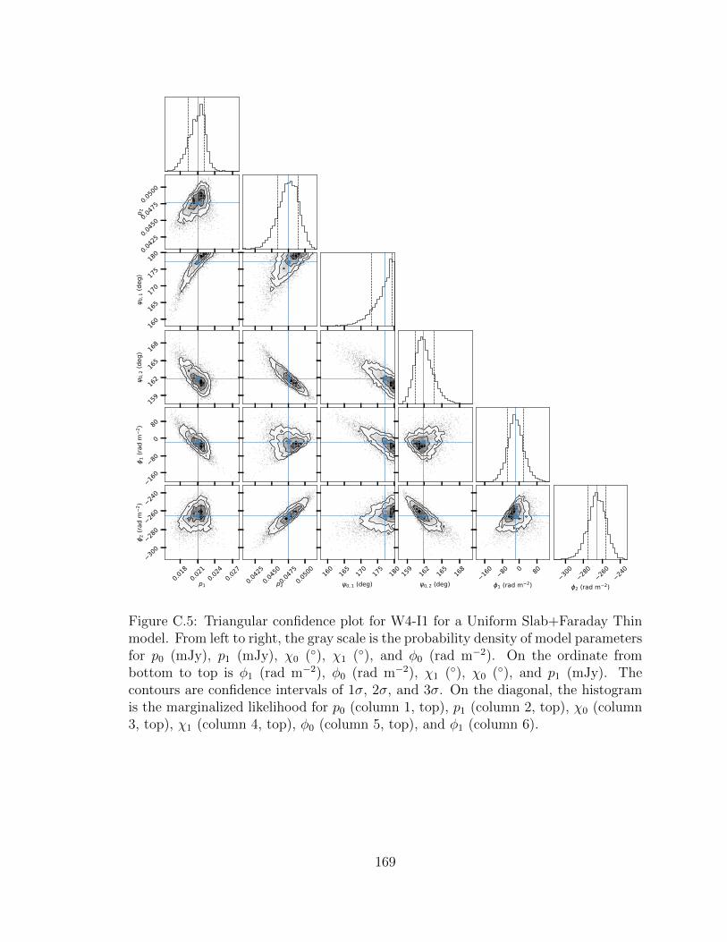
0.042

50.045

00.047

50.050

0

p 2

160

165

170

175

180

0,1 (

deg)

159

162

165

168

0,2 (

deg)

160

80

0

80

1 (ra

d m

2 )

0.018

0.021

0.024

0.027

p1

300

280

260

240

2 (ra

d m

2 )

0.042

50.0

450

0.047

50.0

500

p2

160

165

170

175

180

0, 1 (deg)15

916

216

516

8

0, 2 (deg)16

0 80 0 80

1 (rad m 2)30

028

026

024

0

2 (rad m 2)

Figure C.5: Triangular confidence plot for W4-I1 for a Uniform Slab+Faraday Thinmodel. From left to right, the gray scale is the probability density of model parametersfor p0 (mJy), p1 (mJy), χ0 (), χ1 (), and φ0 (rad m−2). On the ordinate frombottom to top is φ1 (rad m−2), φ0 (rad m−2), χ1 (), χ0 (), and p1 (mJy). Thecontours are confidence intervals of 1σ, 2σ, and 3σ. On the diagonal, the histogramis the marginalized likelihood for p0 (column 1, top), p1 (column 2, top), χ0 (column3, top), χ1 (column 4, top), φ0 (column 5, top), and φ1 (column 6).

169

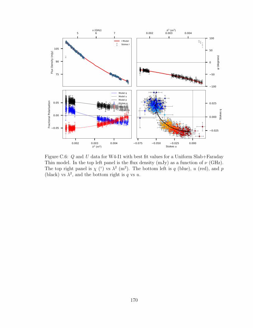
5 6 7 (GHz)

75

90

105Fl

ux D

ensit

y (m

Jy)

I ModelStokes I

0.002 0.003 0.0042 (m2)

0.05

0.00

0.05

Frac

tiona

l Pol

arisa

tion

Model qModel uModel pStokes qStokes uIntensity p

0.002 0.003 0.0042 (m2)

100

50

0

50

100

(deg

rees

)

0.075 0.050 0.025 0.000Stokes u

0.025

0.000

0.025

Stok

es q

Figure C.6: Q and U data for W4-I1 with best fit values for a Uniform Slab+FaradayThin model. In the top left panel is the flux density (mJy) as a function of ν (GHz).The top right panel is χ () vs λ2 (m2). The bottom left is q (blue), u (red), and p(black) vs λ2, and the bottom right is q vs u.

170

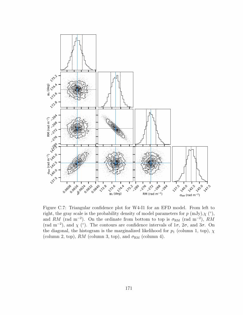
172.8

173.6

174.4

175.2

0 (de

g)

280

276

272

268

264

RM (r

ad m

2 )

0.060

80.0

6160.0

6240.0

6320.0

640

p

137.5

140.0

142.5

145.0

147.5

RM (r

ad m

2 )

172.8

173.6

174.4

175.2

0 (deg)28

027

627

226

826

4

RM (rad m 2)13

7.514

0.014

2.514

5.014

7.5

RM (rad m 2)

Figure C.7: Triangular confidence plot for W4-I1 for an EFD model. From left toright, the gray scale is the probability density of model parameters for p (mJy),χ (),and RM (rad m−2). On the ordinate from bottom to top is σRM (rad m−2), RM(rad m−2), and χ (). The contours are confidence intervals of 1σ, 2σ, and 3σ. Onthe diagonal, the histogram is the marginalized likelihood for p1 (column 1, top), χ(column 2, top), RM (column 3, top), and σRM (column 4).

171

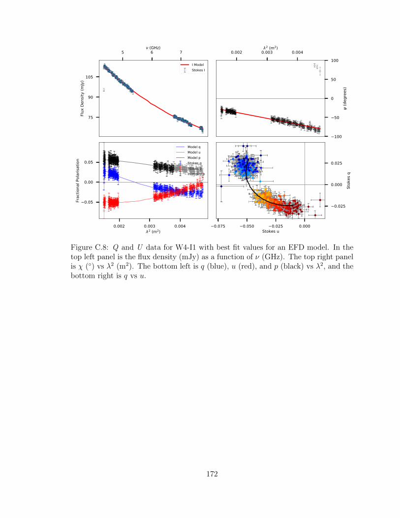
5 6 7 (GHz)

75

90

105Fl

ux D

ensit

y (m

Jy)

I ModelStokes I

0.002 0.003 0.0042 (m2)

0.05

0.00

0.05

Frac

tiona

l Pol

arisa

tion

Model qModel uModel pStokes qStokes uIntensity p

0.002 0.003 0.0042 (m2)

100

50

0

50

100

(deg

rees

)

0.075 0.050 0.025 0.000Stokes u

0.025

0.000

0.025

Stok

es q

Figure C.8: Q and U data for W4-I1 with best fit values for an EFD model. In thetop left panel is the flux density (mJy) as a function of ν (GHz). The top right panelis χ () vs λ2 (m2). The bottom left is q (blue), u (red), and p (black) vs λ2, and thebottom right is q vs u.

172

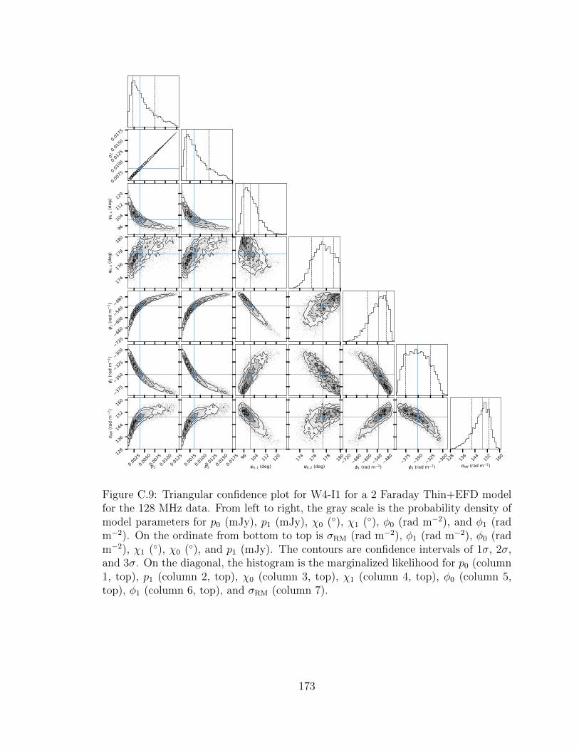
0.007

50.010

00.012

50.015

00.017

5

p 2

9610

411

212

0

0,1 (

deg)

174

176

178

180

0,2 (

deg)

720

660

600

540

480

1 (ra

d m

2 )

375

350

325

300

2 (ra

d m

2 )

0.002

50.0

0500.0

0750.0

1000.0

125

p1

128

136

144

152

160

RM (r

ad m

2 )

0.007

50.0

1000.0

1250.0

1500.0

175

p2

96 104

112

120

0, 1 (deg)17

417

617

818

0

0, 2 (deg)72

066

060

054

048

0

1 (rad m 2)37

535

032

530

0

2 (rad m 2)12

813

614

415

216

0

RM (rad m 2)

Figure C.9: Triangular confidence plot for W4-I1 for a 2 Faraday Thin+EFD modelfor the 128 MHz data. From left to right, the gray scale is the probability density ofmodel parameters for p0 (mJy), p1 (mJy), χ0 (), χ1 (), φ0 (rad m−2), and φ1 (radm−2). On the ordinate from bottom to top is σRM (rad m−2), φ1 (rad m−2), φ0 (radm−2), χ1 (), χ0 (), and p1 (mJy). The contours are confidence intervals of 1σ, 2σ,and 3σ. On the diagonal, the histogram is the marginalized likelihood for p0 (column1, top), p1 (column 2, top), χ0 (column 3, top), χ1 (column 4, top), φ0 (column 5,top), φ1 (column 6, top), and σRM (column 7).

173

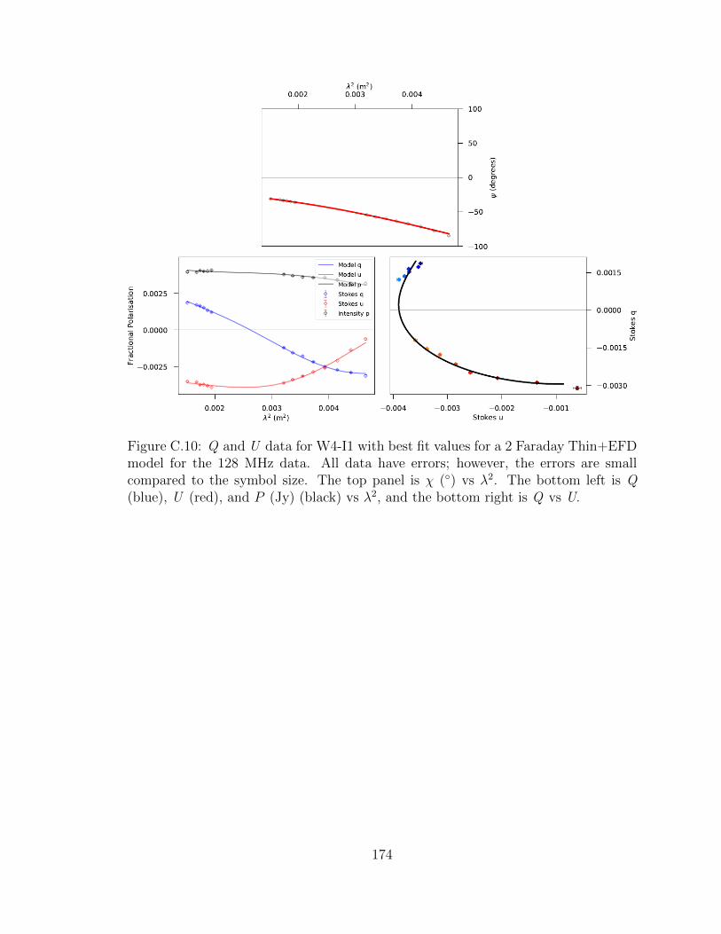
Figure C.10: Q and U data for W4-I1 with best fit values for a 2 Faraday Thin+EFDmodel for the 128 MHz data. All data have errors; however, the errors are smallcompared to the symbol size. The top panel is χ () vs λ2. The bottom left is Q(blue), U (red), and P (Jy) (black) vs λ2, and the bottom right is Q vs U.

174

Bibliography

Albert, J. et al. 2008, ApJ, 684, 1351, 0801.3150

Anantharamaiah, K. R. 1985, Journal of Astrophysics and Astronomy, 6, 203

Anderson, C. S., Gaensler, B. M., Feain, I. J., & Franzen, T. M. O. 2015, ApJ, 815,

49, 1511.04080

Anderson, L. D., Bania, T. M., Balser, D. S., Cunningham, V., Wenger, T. V.,

Johnstone, B. M., & Armentrout, W. P. 2014, ApJS, 212, 1, 1312.6202

Anderson, L. D., Zavagno, A., Barlow, M. J., Garcıa-Lario, P., & Noriega-Crespo, A.

2012, A&A, 537, A1, 1110.3303

Aragona, C., McSwain, M. V., Grundstrom, E. D., Marsh, A. N., Roettenbacher,

R. M., Hessler, K. M., Boyajian, T. S., & Ray, P. S. 2009, ApJ, 698, 514, 0902.4015

Balser, D. S., Anish Roshi, D., Jeyakumar, S., Bania, T. M., Montet, B. T., &

Shitanishi, J. A. 2016, ApJ, 816, 22, 1511.07383

Basu, S., Johnstone, D., & Martin, P. G. 1999, ApJ, 516, 843, astro-ph/9812283

Bell, M. R., & Enßlin, T. A. 2012, A&A, 540, A80, 1112.4175

Berghofer, T. W., & Christian, D. J. 2002, A&A, 384, 890

Bignami, G. F., Caraveo, P. A., Lamb, R. C., Markert, T. H., & Paul, J. A. 1981,

ApJ, 247, L85

Bignell, C. 1982, in Synthesis Mapping, ed. A. R. Thompson & L. R. D’Addario, 6

Bik, A. et al. 2012, ApJ, 744, 87, 1109.3467

175

Blitz, L., Fich, M., & Stark, A. A. 1982, ApJS, 49, 183

Bouret, J.-C., Hillier, D. J., Lanz, T., & Fullerton, A. W. 2012, A&A, 544, A67,

1205.3075

Bouret, J.-C., Lanz, T., & Hillier, D. J. 2005, A&A, 438, 301, astro-ph/0412346

Braunsfurth, E. 1983, A&A, 117, 297

Breitschwerdt, D., & Kahn, F. D. 1988, MNRAS, 235, 1011

Brentjens, M. A., & de Bruyn, A. G. 2005, A&A, 441, 1217, astro-ph/0507349

Brogan, C. L., Troland, T. H., Roberts, D. A., & Crutcher, R. M. 1999, ApJ, 515,

304, astro-ph/9711014

Brown, J. C., Taylor, A. R., & Jackel, B. J. 2003, ApJS, 145, 213

Brown, S. 2011

Buchner, J. et al. 2014, A&A, 564, A125, 1402.0004

Burn, B. J. 1966, MNRAS, 133, 67

Carpenter, J. M., Heyer, M. H., & Snell, R. L. 2000, ApJS, 130, 381, astro-ph/0005237

Casares, J., Ribas, I., Paredes, J. M., Martı, J., & Allende Prieto, C. 2005, MNRAS,

360, 1105, astro-ph/0504332

Celnik, W. E. 1983, A&AS, 53, 403

——. 1985, A&A, 144, 171

——. 1986, A&A, 160, 287

Chlebowski, T., & Garmany, C. D. 1991, ApJ, 368, 241

176

Churchwell, E. et al. 2006, ApJ, 649, 759

Cioffi, D. F., & Jones, T. W. 1980, AJ, 85, 368

Condon, J. J., Cotton, W. D., Greisen, E. W., Yin, Q. F., Perley, R. A., Taylor,

G. B., & Broderick, J. J. 1998, AJ, 115, 1693

Costa, A. H., & Spangler, S. R. 2018, ArXiv e-prints, 1803.02878

Costa, A. H., Spangler, S. R., Sink, J. R., Brown, S., & Mao, S. A. 2016, ApJ, 821,

92, 1510.04664

Dambis, A. K., Mel’Nik, A. M., & Rastorguev, A. S. 2001, Astronomy Letters, 27, 58

de Avillez, M. A., & Breitschwerdt, D. 2005, A&A, 436, 585, astro-ph/0502327

De Marco, O., & Schmutz, W. 1999, A&A, 345, 163

Dennison, B., Topasna, G. A., & Simonetti, J. H. 1997, ApJ, 474, L31

Dhawan, V., Mioduszewski, A., & Rupen, M. 2006, in VI Microquasar Workshop:

Microquasars and Beyond, 52.1

Dickel, H. R. 1980, ApJ, 238, 829

Dickel, H. R., Dickel, J. R., Wilson, W. J., & Werner, M. W. 1980, ApJ, 237, 711

Digel, S. W., Lyder, D. A., Philbrick, A. J., Puche, D., & Thaddeus, P. 1996, ApJ,

458, 561

Draine, B. T. 2011, Physics of the Interstellar and Intergalactic Medium

Dubus, G. 2006, A&A, 456, 801, astro-ph/0605287

Everett, J. E., & Weisberg, J. M. 2001, ApJ, 553, 341, astro-ph/0009266

Farnsworth, D., Rudnick, L., & Brown, S. 2011, AJ, 141, 191, 1103.4149

177

Feigelson, E. D., & Townsley, L. K. 2008, ApJ, 673, 354, 0710.0090

Feigelson, E. D. et al. 2013, ApJS, 209, 26, 1309.4483

Feroz, F., Hobson, M. P., & Bridges, M. 2009, MNRAS, 398, 1601, 0809.3437

Ferriere, K. 2011, Mem. Soc. Astron. Italiana, 82, 824

Ferriere, K. M., Mac Low, M.-M., & Zweibel, E. G. 1991, ApJ, 375, 239

Foster, T., & Brunt, C. M. 2015, AJ, 150, 147, 1405.7003

Frail, D. A., & Hjellming, R. M. 1991, AJ, 101, 2126

Franzen, T. M. O. et al. 2014, MNRAS, 439, 1212, 1312.2301

Gao, X. Y., Reich, W., Reich, P., Han, J. L., & Kothes, R. 2015, A&A, 578, A24,

1504.00142

Garmany, C. D. 1988, NASA Special Publication, 497, 160

Getman, K. V., Feigelson, E. D., Garmire, G., Broos, P., & Wang, J. 2007, ApJ, 654,

316, astro-ph/0607006

Gooch, R. 1995, in Astronomical Society of the Pacific Conference Series, Vol. 77,

Astronomical Data Analysis Software and Systems IV, ed. R. A. Shaw, H. E. Payne,

& J. J. E. Hayes, 144

Gordon, C., & Trotta, R. 2007, MNRAS, 382, 1859, 0706.3014

Graham, D. A., Haslam, C. G. T., Salter, C. J., & Wilson, W. E. 1982, A&A, 109,

145

Gray, A. D., Landecker, T. L., Dewdney, P. E., Taylor, A. R., Willis, A. G., &

Normandeau, M. 1999, ApJ, 514, 221, astro-ph/9812164

178

Gregory, P. C. 2005, Bayesian Logical Data Analysis for the Physical Sciences: A

Comparative Approach with ‘Mathematica’ Support (Cambridge University Press)

Gregory, P. C., & Neish, C. 2002, ApJ, 580, 1133

Gregory, P. C. et al. 1979, AJ, 84, 1030

Groenewegen, M. A. T., Lamers, H. J. G. L. M., & Pauldrach, A. W. A. 1989, A&A,

221, 78

Guetter, H. H., & Vrba, F. J. 1989, AJ, 98, 611

Gurnett, D. A., & Bhattacharjee, A. 2005, Introduction to Plasma Physics

Han, J. L., Manchester, R. N., Lyne, A. G., Qiao, G. J., & van Straten, W. 2006,

ApJ, 642, 868, astro-ph/0601357

Harvey-Smith, L., Madsen, G. J., & Gaensler, B. M. 2011, ApJ, 736, 83, 1106.0931

Hasegawa, T., Sato, F., & Fukui, Y. 1983, AJ, 88, 658

Haverkorn, M., Gaensler, B. M., McClure-Griffiths, N. M., Dickey, J. M., & Green,

A. J. 2004, ApJ, 609, 776, arXiv:astro-ph/0403655

Heald, G. 2009, in IAU Symposium, Vol. 259, IAU Symposium, ed. K. G. Strassmeier,

A. G. Kosovichev, & J. E. Beckman, 591–602

Heiles, C., & Chu, Y.-H. 1980, ApJ, 235, L105

Heiles, C., Chu, Y.-H., & Troland, T. H. 1981, ApJ, 247, L77

Herter, T., Briotta, Jr., D. A., Gull, G. E., Shure, M. A., & Houck, J. R. 1982, ApJ,

262, 164

Heyer, M. H. et al. 1996, ApJ, 464, L175

179

Heyer, M. H., & Terebey, S. 1998, ApJ, 502, 265

Hill, A. S. et al. 2017, MNRAS, 467, 4631, 1702.02200

Hollenbach, D. J., & Tielens, A. G. G. M. 1999, Reviews of Modern Physics, 71, 173

Howarth, I. D., & Prinja, R. K. 1989, ApJS, 69, 527

Jose, J., Kim, J. S., Herczeg, G. J., Samal, M. R., Bieging, J. H., Meyer, M. R., &

Sherry, W. H. 2016, ApJ, 822, 49, 1602.06212

Kassim, N. E., Weiler, K. W., Erickson, W. C., & Wilson, T. L. 1989, ApJ, 338, 152

Kellermann, K. I., Pauliny-Toth, I. I. K., & Williams, P. J. S. 1969, ApJ, 157, 1

Kharchenko, N. V., Piskunov, A. E., Roser, S., Schilbach, E., & Scholz, R.-D. 2005,

A&A, 438, 1163, astro-ph/0501674

Kiminki, M. M., Kim, J. S., Bagley, M. B., Sherry, W. H., & Rieke, G. H. 2015, ApJ,

813, 42, 1509.00081

Kortgen, B., & Banerjee, R. 2015, MNRAS, 451, 3340, 1502.03306

Lagrois, D., & Joncas, G. 2009a, ApJ, 691, 1109

——. 2009b, ApJ, 693, 186

Lagrois, D., Joncas, G., & Drissen, L. 2012, MNRAS, 420, 2280, 1112.3327

Landecker, T. L. et al. 2010, A&A, 520, A80, 1004.2536

Law, C. J. et al. 2011, ApJ, 728, 57, 1012.0945

Lestrade, J.-F., Preston, R. A., Jones, D. L., Phillips, R. B., Rogers, A. E. E., Titus,

M. A., Rioja, M. J., & Gabuzda, D. C. 1999, A&A, 344, 1014

180

Macquart, J.-P., Ekers, R. D., Feain, I., & Johnston-Hollitt, M. 2012, ApJ, 750, 139,

1203.2706

Massey, P., Johnson, K. E., & Degioia-Eastwood, K. 1995, ApJ, 454, 151

Massi, M. 2004, A&A, 422, 267, astro-ph/0404605

Massi, M., Migliari, S., & Chernyakova, M. 2017, MNRAS, 468, 3689, 1704.01335

Massi, M., Ribo, M., Paredes, J. M., Garrington, S. T., Peracaula, M., & Martı, J.

2004, A&A, 414, L1, astro-ph/0312091

Megier, A., Strobel, A., Galazutdinov, G. A., & Kre lowski, J. 2009, A&A, 507, 833

Menon, T. K. 1962, ApJ, 135, 394

Minter, A. H., & Spangler, S. R. 1996, ApJ, 458, 194

Mokiem, M. R. et al. 2007, A&A, 473, 603, 0708.2042

Moore, T. J. T., Bretherton, D. E., Fujiyoshi, T., Ridge, N. A., Allsopp, J., Hoare,

M. G., Lumsden, S. L., & Richer, J. S. 2007, MNRAS, 379, 663, 0705.0642

Nakano, M. et al. 2017, PASJ, 69, 16, 1611.06702

Nakano, M., Sugitani, K., Watanabe, M., Fukuda, N., Ishihara, D., & Ueno, M. 2012,

AJ, 143, 61, 1201.2761

Navarete, F., Figueredo, E., Damineli, A., Moises, A. P., Blum, R. D., & Conti, P. S.

2011, AJ, 142, 67, 1106.2770

Normandeau, M., Taylor, A. R., & Dewdney, P. E. 1996, Nature, 380, 687

——. 1997, ApJS, 108, 279

181

Oey, M. S., Watson, A. M., Kern, K., & Walth, G. L. 2005, AJ, 129, 393, astro-

ph/0501136

Osterbrock, D., & Flather, E. 1959, ApJ, 129, 26

O’Sullivan, S. P. et al. 2012, MNRAS, 421, 3300, 1201.3161

Paredes, J. M., Ribo, M., Bosch-Ramon, V., West, J. R., Butt, Y. M., Torres, D. F.,

& Martı, J. 2007, ApJ, 664, L39, 0706.0877

Park, B.-G., & Sung, H. 2002, AJ, 123, 892

Pasetto, A., Carrasco-Gonzalez, C., O’Sullivan, S., Basu, A., Bruni, G., Kraus, A.,

Curiel, S., & Mack, K.-H. 2018, ArXiv e-prints, 1801.09731

Passot, T., Vazquez-Semadeni, E., & Pouquet, A. 1995, ApJ, 455, 536, astro-

ph/9601182

Pavel, M. D., & Clemens, D. P. 2012, ApJ, 760, 150, 1210.4079

Pellegrini, E. W. et al. 2007, ApJ, 658, 1119, astro-ph/0611808

Perez, M. R., Joner, M. D., The, P. S., & Westerlund, B. E. 1989, PASP, 101, 195

Planck Collaboration et al. 2015, ArXiv e-prints, 1501.00922

Purcell, C. R. et al. 2015, ApJ, 804, 22, 1502.06296

Quireza, C., Rood, R. T., Bania, T. M., Balser, D. S., & Maciel, W. J. 2006, ApJ,

653, 1226, astro-ph/0609006

Reynolds, R. J., Sterling, N. C., & Haffner, L. M. 2001, ApJ, 558, L101, astro-

ph/0108046

Roberts, D. A., Crutcher, R. M., Troland, T. H., & Goss, W. M. 1993, ApJ, 412, 675

182

Rodrıguez, L. F., Gomez, Y., & Tafoya, D. 2012, MNRAS, 420, 279, 1110.4679

Roman-Zuniga, C. G., & Lada, E. A. 2008, Star Formation in the Rosette Complex,

ed. B. Reipurth, 928

Roman-Zuniga, C. G., Ybarra, J. E., Megıas, G. D., Tapia, M., Lada, E. A., & Alves,

J. F. 2015, AJ, 150, 80, 1507.00016

Roshi, D. A. 2007, ApJ, 658, L41, astro-ph/0702150

Sato, F. 1990, AJ, 99, 1897

Savage, A. H., Spangler, S. R., & Fischer, P. D. 2013, ApJ, 765, 42

Shi, H. M., & Hu, J. Y. 1999, A&AS, 136, 313

Shull, J. M., & van Steenberg, M. E. 1985, ApJ, 294, 599

Sokoloff, D. D., Bykov, A. A., Shukurov, A., Berkhuijsen, E. M., Beck, R., & Poezd,

A. D. 1998, MNRAS, 299, 189

Sota, A., Maız Apellaniz, J., Walborn, N. R., Alfaro, E. J., Barba, R. H., Morrell,

N. I., Gamen, R. C., & Arias, J. I. 2011, ApJS, 193, 24, 1101.4002

Sota, A., Maız Apellaniz, J., Walborn, N. R., & Shida, R. Y. 2008, in Revista Mexi-

cana de Astronomia y Astrofisica Conference Series, Vol. 33, Revista Mexicana de

Astronomia y Astrofisica Conference Series, 56–56, astro-ph/0703005

Spangler, S. R., & Cordes, J. M. 1998, ApJ, 505, 766

Stil, J., Wityk, N., Ouyed, R., & Taylor, A. R. 2009, ApJ, 701, 330, 0807.0057

Straizys, V., Kazlauskas, A., Vansevicius, V., & Cernis, K. 1993, Baltic Astronomy,

2, 171

183

Sun, X. H., Han, J. L., Reich, W., Reich, P., Shi, W. B., Wielebinski, R., & Furst,

E. 2007, A&A, 463, 993, astro-ph/0611622

Sun, X. H. et al. 2015, ApJ, 811, 40, 1508.03889

Sun, X. H., Reich, W., Waelkens, A., & Enßlin, T. A. 2008, A&A, 477, 573, 0711.1572

Taylor, A. R. et al. 2003, AJ, 125, 3145

Taylor, A. R., Irwin, J. A., Matthews, H. E., & Heyer, M. H. 1999, ApJ, 513, 339

Taylor, A. R., Stil, J. M., & Sunstrum, C. 2009, ApJ, 702, 1230

Terebey, S., Fich, M., Taylor, R., Cao, Y., & Hancock, T. 2003, ApJ, 590, 906

Tielens, A. G. G. M., & Hollenbach, D. 1985, ApJ, 291, 722

Tomisaka, K. 1990, ApJ, 361, L5

——. 1998, MNRAS, 298, 797, astro-ph/9804029

Townsley, L. K., Broos, P. S., Garmire, G. P., Bouwman, J., Povich, M. S., Feigelson,

E. D., Getman, K. V., & Kuhn, M. A. 2014, ApJS, 213, 1, 1403.2576

Troland, T. H., Goss, W. M., Brogan, C. L., Crutcher, R. M., & Roberts, D. A. 2016,

ApJ, 825, 2, 1605.04799

Trotta, R. 2008, Contemporary Physics, 49, 71, 0803.4089

Vallee, J. P. 1993, ApJ, 419, 670

van der Werf, P. P., & Goss, W. M. 1990, A&A, 238, 296

Van Eck, C. L. et al. 2011, ApJ, 728, 97, 1012.2938

van Marle, A. J., Meliani, Z., & Marcowith, A. 2015, A&A, 584, A49, 1509.00192

184

Walch, S., Whitworth, A. P., Bisbas, T. G., Hubber, D. A., & Wunsch, R. 2015,

MNRAS, 452, 2794

Wang, J., Townsley, L. K., Feigelson, E. D., Broos, P. S., Getman, K. V., Roman-

Zuniga, C. G., & Lada, E. 2008, ApJ, 675, 464, 0711.2024

Watson, C. et al. 2008, ApJ, 681, 1341, 0806.0609

Weaver, R., McCray, R., Castor, J., Shapiro, P., & Moore, R. 1977, ApJ, 218, 377

Wendker, H. 1968, ZAp, 68, 368

West, J. L., English, J., Normandeau, M., & Landecker, T. L. 2007, ApJ, 656, 914,

arXiv:astro-ph/0611226

Whiting, C. A., Spangler, S. R., Ingleby, L. D., & Haffner, L. M. 2009, ApJ, 694,

1452, 0802.0481

Woermann, B., Gaylard, M. J., & Otrupcek, R. 2001, MNRAS, 325, 1213

Zamora-Aviles, M., Vazquez-Semadeni, E., Kortgen, B., Banerjee, R., & Hartmann,

L. 2018, MNRAS, 474, 4824

185