A stochastic sediment delivery model for a steep Mediterranean

landscape

Emmanuel J. Gabet

Department of Geology, University of Montana, Missoula, Montana, USA

Thomas Dunne

Donald Bren School of Environmental Science and Management and Department of Geological Sciences, University ofCalifornia, Santa Barbara, Santa Barbara, California, USA

Received 20 May 2003; accepted 17 June 2003; published 6 September 2003.

[1] It is a truism in geomorphology that climatic events operate on a landscape to drivesediment transport processes, yet few investigations have formally linked climate andterrain characteristics with geomorphological processes. In this study, we incorporatesediment transport equations derived from fieldwork into a computer model that predictsthe delivery of sediment from hillslopes in a steep Mediterranean landscape near SantaBarbara, California. The sediment transport equations are driven by rainstorms and firesthat are stochastically generated from probability distributions. The model is used tocompare the rates and processes of sediment delivery under two vegetation types: coastalsage scrub and grasslands. Conversion of vegetation from sage to exotic grasses is acommon land management strategy in the region and may also be engendered by regionalclimate change due to global warming. Results from the model suggest that(1) approximately 40% more sediment is delivered from grasslands (98 t km�2 yr�1) thanthe sage scrub (71 t km�2 yr�1) and (2) chronic soil creep processes dominate undergrasslands whereas catastrophic processes dominate under coastal sage scrub. Resultsfrom the model also suggest that changes in the spatial distribution of vegetation arisingfrom climate change will have a greater effect on sediment delivery than changes in themagnitude and frequency of meteorological events. INDEX TERMS: 1824 Hydrology:

Geomorphology (1625); 1815 Hydrology: Erosion and sedimentation; 1803 Hydrology: Anthropogenic

effects; 1869 Hydrology: Stochastic processes; KEYWORDS: geomorphology, landslides, erosion, fire,

hillslopes, semiarid

Citation: Gabet, E. J., and T. Dunne, A stochastic sediment delivery model for a steep Mediterranean landscape, Water Resour. Res.,

39(9), 1237, doi:10.1029/2003WR002341, 2003.

1. Introduction

1.1. Background

[2] With frequent fires, infrequent but intense rainfall,and sparse vegetative cover, the delivery of sediment fromhillslopes in hilly Mediterranean landscapes is stronglyepisodic [Rice, 1982]. Whether sediment is delivered as asteady trickle or as large pulses can affect a wide range ofgeomorphic processes. For example, sediment delivery maycome in the form of debris flows, which can cause signif-icant property damage and the loss of life. Sedimentproduction from hillslopes may overwhelm the transportcapacity of the fluvial network and lead to flooding as wellas the destruction of riverine habitats. Finally, over geolog-ical timescales, the frequency and magnitude of sedimentdelivery may control rates of bedrock incision [Sklar andDietrich, 1998].[3] In the absence of anthropogenic disturbances, climate

ultimately determines the nature of sediment delivery.Climate regulates sediment production directly throughmeteorological events and, indirectly, by controlling the

distribution of vegetation communities. For example,sediment transport by tree-throw contributes to soil creepin forested regions [Denny and Goodlett, 1956; Gabet etal., 2003] but is not relevant in areas that are too dry fortrees to grow. The influence of climate on the spatialpattern of vegetation communities, however, may beoverridden by anthropogenic modifications. Indeed, in theSouthwest United States, hillslopes are often cleared ofbrush and converted to grasslands. This conversion isusually done to increase forage for livestock [Rice andFoggin, 1971] but may also be done to reduce fire hazardsand increase water yields [Hibbert, 1971]. A well-docu-mented result of this land management strategy has been anincrease in the frequency of landsliding on converted hill-slopes [Corbett and Rice, 1966; Bailey and Rice, 1969;Rice and Foggin, 1971; Terwilliger and Waldron, 1991;Gabet and Dunne, 2002]. In light of predictions that under awarmer climate, the distribution of grasslands in Californiawill increase at the expense of shrub communities [Field etal., 1999], the effects of this management strategy maypresage an underappreciated consequence of global climatechange.[4] A fundamental tenet in geomorphology holds that

climatic events operating on a landscape drive sedimentCopyright 2003 by the American Geophysical Union.0043-1397/03/2003WR002341$09.00

ESG 2 - 1

WATER RESOURCES RESEARCH, VOL. 39, NO. 9, 1237, doi:10.1029/2003WR002341, 2003

transport processes and hillslope evolution. Rice [1982]proposed a conceptual model that recognizes the stochasticnature of rainstorms and fires and their effects on shallowlandslides, but, to date, few studies have formally (i.e.,mathematically) linked climate and sediment transport.Kirkby [1976] applied a frequency distribution of dailyrainfall to drive a process-based, hillslope hydrology model.With this model, he predicted annual runoff and related it torates of sediment transport to model the evolution of hill-slope profiles. Dunne [1991] demonstrated how variationsin the frequency distributions of rainfall intensity andduration alter both the temporal pattern of sediment fluxfrom hillslopes and the shape of hillslope profiles. Dunne[1991] also illustrated how the stochastic nature of climateis related to the spatial and temporal distribution of land-sliding in the Pacific Northwest. Benda and Dunne [1997a,1997b] furthered this approach with a process-based modelof bedrock hollow-filling and landslide initiation. Theirmodel combines random sequences of rainstorms and firesdrawn from probability density functions (pdf’s) with alandscape defined by a spatial distribution of characteristics(e.g., hillslope gradient, soil depth) also described by pdf’s.Iida [1999] demonstrated the utility of rainfall pdf’s forpredicting the susceptibility of slopes to shallow landslid-ing. Finally, Tucker and Bras [2000] modeled the effects ofrainfall variability on the evolution of drainage basins,illustrating that erosional thresholds can have morphologicalconsequences.[5] In this contribution, we expand upon the approach

presented by Benda and Dunne [1997a, 1997b] and apply itto a hilly, semiarid watershed with a Mediterranean climateand two vegetation communities. The model proposed hereincludes all the dominant processes that we observed over aperiod of 5 years that encompassed a fire and the highestrecorded annual rainfall in the region. The governingequations for the sediment transport processes have beendeveloped and calibrated through fieldwork, and we assumethat we have not overlooked any important process. Withthis model, we explore the effects of vegetation conversionand climate change on sediment production.

1.2. Field Area and Sediment Transport Processes

[6] The fieldwork and modeling efforts are centered on ahilly watershed in Sedgwick Reserve in the Santa YnezValley, near Santa Barbara, California (Figure 1). Located inthe western portion of the Transverse Ranges, the field siteis underlain by the Paso Robles Formation, a Pliestocenefanglomerate shed from the ancestral San Rafael Range[Dibblee, 1993]. The Paso Robles has been incised toproduce gentle to steep rolling hillslopes with slope anglesup to 45� and relief ranging from 30 to 50 m. The climate isMediterranean with an average annual rainfall of 50 cm. Thetwo main vegetation communities are coastal sage scrub(primarily Artemisia californica and Salvia leucophylla)and exotic grasses (various species of Bromus and Avena).Presently, grazing occurs on the grasslands at relatively lowstocking rates (40 cow days ha�1 yr�1).[7] Few of the lower-order valleys at Sedgwick have

channels, and there is approximately 1 m of fill in thefirst-order valleys. Little is known about the regionalhistory, but presumably, the valleys began to fill withcolluvium sometime after the region emerged from thelatest glacial maximum, 16,500 years B.P. [Kennett and

Ingram, 1995]. Under the drier conditions, the hillslopesediment delivery processes may have gained an advantageover the fluvial sediment transport processes. There isevidence that the channel network is beginning to expandafter this phase of contraction. A knickpoint has beenadvancing up the main channel, Figueroa Creek, andtributary knickpoints are just beginning to form where themain knickpoint has moved past tributary valleys.[8] Sediment is delivered to the valley bottoms at Sedg-

wick Reserve by three types of processes. The first, soil creep(sensu lato), includes bioturbation [Gabet, 2000] and dryravel [Gabet, 2003b]. Second, sediment may be delivered byshallow landslides issuing from bedrock hollows [Gabet andDunne, 2002]. Hollows accumulate sediment from adjacenthillslopes, and as the soil in a hollow thickens over time, itbecomes increasingly susceptible to fail as a shallow land-slide during heavy rainfall [Campbell, 1975; Dietrich andDunne, 1978]. Fire may increase the likelihood of failure bydestroying vegetation that increases soil strength throughroot cohesion. When a hollow is evacuated, it fills up againand the cycle repeats itself. The third important sedimentdelivery mechanism in this landscape is by thin debris flow(TDF) [Wells, 1987;Gabet, 2003a]. This process is limited tosage scrub vegetation and occurs when waxy organic mole-cules, vaporized during a fire from burning vegetation,recondense within the soil. This hydrophobic layer, deposited1–2 cm below the soil surface, leads to a shallow perchedwater table during rainstorms. If pore pressures within thislayer become sufficiently high, TDFs are triggered, strippingthe top layer of soil [Wells, 1987; Gabet, 2003a]. Fieldobservations indicate that the sediment flux from TDFs andthe soil creep processes are not limited by the supply ofsediment.[9] Field observations and an extensive program of

rainfall simulation experiments on plots that had undergonea variety of different treatments (i.e., trampled, burnt,

Figure 1. Site map for Sedgwick Reserve.

ESG 2 - 2 GABET AND DUNNE: A STOCHASTIC SEDIMENT DELIVERY MODEL

mechanically denuded) suggest that overland flow does notappear to be an important transport process in either thesage or the grasslands. Infiltration capacities in the sage aresufficiently high to prevent the generation of Horton over-land flow [Fierer and Gabet, 2002]. Even after a series ofstorms delivered rainfall to burnt hillslopes in the sage andtriggered TDFs [Gabet, 2003a], there was no evidence ofsediment transport by overland flow (e.g., the presence ofrills or delta-like deposits of fine-grained material at thebase of the slopes). In the grasslands, sediment transport bysurface runoff is limited by the detachment of soil particlesby raindrop impact [Gabet and Dunne, 2003]. Because thegrazing pressure at Sedgwick Reserve is relatively light,the vegetation cover remains sufficiently high to shield theground surface so that the annual sediment loss by overlandflow is estimated to be 3–4 orders of magnitude less thanby biogenic soil creep. This estimate is supported byobservations made by the Sedgwick Reserve manager,who reported seeing clear water flowing down the hillslopesduring intense rainfall (M. Williams, personal communica-tion, 2001). Additionally, we did not observe any evidenceof significant sediment transport from overland flow (e.g.,

rill formation or fine-grained deposits) on burnt grasslandslopes.

2. Model Description

2.1. Model Domain

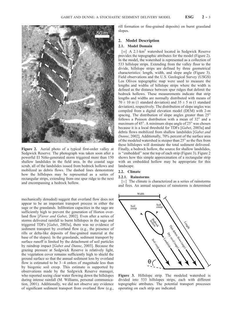
[10] A 2.1-km2 watershed located in Sedgwick Reserveprovides the topographic attributes for the model (Figure 2).In the model, the watershed is represented as a collection of533 hillslope strips. Extending from the valley floor to thedivide, hillslope strips are defined by three geometricalcharacteristics: length, width, and slope angle (Figure 3).Field observations and the U.S. Geological Survey (USGS)Los Olivos topographic map were used to measure thelengths and widths of hillslope strips where the width isdefined as the distance between spur ridges that delimit thebedrock hollows. These measurements indicate that striplengths and widths are normally distributed with means of70 ± 10 m (1 standard deviation) and 35 ± 5 m (1 standarddeviation), respectively. The distribution of slope angles wascompiled from a digital elevation model (DEM) with 2-mspacing. The distribution of slope angles greater than 25�follows a Poisson distribution with a mean of 32� and amaximum of 45�. A minimum slope angle of 25�was chosenbecause it is a local threshold for TDFs [Gabet, 2003a] anddebris flows mobilized from shallow landslides [Gabet andDunne, 2002]. Additionally, 70% percent of the surface areaof the modeled watershed is steeper than 25� so the flux fromthese hillslopes will dominate the total sediment delivered.Finally, a bedrock hollow, the source for shallow landslides,is ‘‘embedded’’ near the top of each strip (Figure 3). Figure 2shows how this simple approximation of a rectangular stripwith an embedded hollow may be appropriate for thislandscape.

2.2. Climate

2.2.1. Rainstorms[11] The climate is characterized as a series of rainstorms

and fires. An annual sequence of rainstorms is determined

Figure 2. Aerial photo of a typical first-order valley atSedgwick Reserve. The photograph was taken soon after apowerful El Nino-generated storm triggered more than 150shallow landslides in the field area. In the coastal sagescrub, all of the landslides issued from bedrock hollows andmobilized as debris flows. The dashed lines demonstratehow the hillslopes may be represented as a series ofrectangular strips, extending from one spur ridge to the nextand encompassing a bedrock hollow.

Figure 3. Hillslope strip. The modeled watershed isdivided into 533 hillslopes strips, each with differenttopographic attributes. The potential transport processesoperating on each strip are indicated.

GABET AND DUNNE: A STOCHASTIC SEDIMENT DELIVERY MODEL ESG 2 - 3

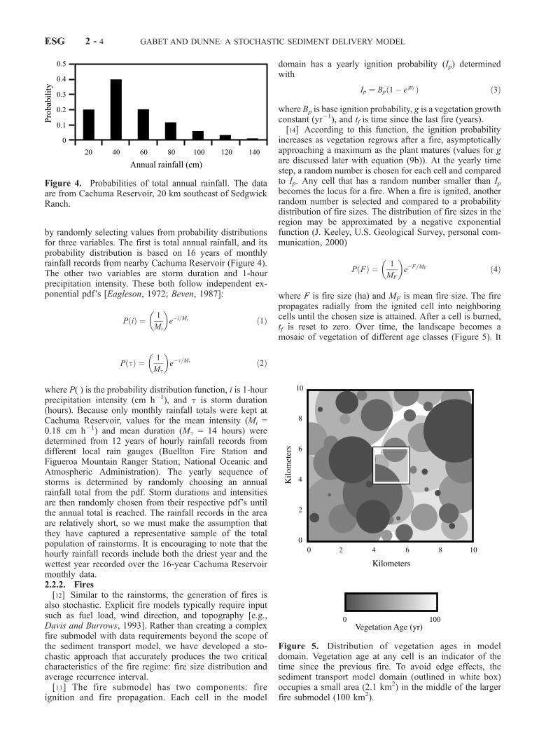
by randomly selecting values from probability distributionsfor three variables. The first is total annual rainfall, and itsprobability distribution is based on 16 years of monthlyrainfall records from nearby Cachuma Reservoir (Figure 4).The other two variables are storm duration and 1-hourprecipitation intensity. These both follow independent ex-ponential pdf’s [Eagleson, 1972; Beven, 1987]:

P ið Þ ¼ 1

Mi

� �e�i=Mi ð1Þ

P tð Þ ¼ 1

Mt

� �e�t=Mt ð2Þ

where P( ) is the probability distribution function, i is 1-hourprecipitation intensity (cm h�1), and t is storm duration(hours). Because only monthly rainfall totals were kept atCachuma Reservoir, values for the mean intensity (Mi =0.18 cm h�1) and mean duration (Mt = 14 hours) weredetermined from 12 years of hourly rainfall records fromdifferent local rain gauges (Buellton Fire Station andFigueroa Mountain Ranger Station; National Oceanic andAtmospheric Administration). The yearly sequence ofstorms is determined by randomly choosing an annualrainfall total from the pdf. Storm durations and intensitiesare then randomly chosen from their respective pdf’s untilthe annual total is reached. The rainfall records in the areaare relatively short, so we must make the assumption thatthey have captured a representative sample of the totalpopulation of rainstorms. It is encouraging to note that thehourly rainfall records include both the driest year and thewettest year recorded over the 16-year Cachuma Reservoirmonthly data.2.2.2. Fires[12] Similar to the rainstorms, the generation of fires is

also stochastic. Explicit fire models typically require inputsuch as fuel load, wind direction, and topography [e.g.,Davis and Burrows, 1993]. Rather than creating a complexfire submodel with data requirements beyond the scope ofthe sediment transport model, we have developed a sto-chastic approach that accurately produces the two criticalcharacteristics of the fire regime: fire size distribution andaverage recurrence interval.[13] The fire submodel has two components: fire

ignition and fire propagation. Each cell in the model

domain has a yearly ignition probability (Ip) determinedwith

Ip ¼ Bp 1� e gtfð Þ ð3Þ

where Bp is base ignition probability, g is a vegetation growthconstant (yr�1), and tf is time since the last fire (years).[14] According to this function, the ignition probability

increases as vegetation regrows after a fire, asymptoticallyapproaching a maximum as the plant matures (values for gare discussed later with equation (9b)). At the yearly timestep, a random number is chosen for each cell and comparedto Ip. Any cell that has a random number smaller than Ipbecomes the locus for a fire. When a fire is ignited, anotherrandom number is selected and compared to a probabilitydistribution of fire sizes. The distribution of fire sizes in theregion may be approximated by a negative exponentialfunction (J. Keeley, U.S. Geological Survey, personal com-munication, 2000)

P Fð Þ ¼ 1

MF

� �e�F=MF ð4Þ

where F is fire size (ha) and MF is mean fire size. The firepropagates radially from the ignited cell into neighboringcells until the chosen size is attained. After a cell is burned,tf is reset to zero. Over time, the landscape becomes amosaic of vegetation of different age classes (Figure 5). It

Figure 4. Probabilities of total annual rainfall. The dataare from Cachuma Reservoir, 20 km southeast of SedgwickRanch.

Figure 5. Distribution of vegetation ages in modeldomain. Vegetation age at any cell is an indicator of thetime since the previous fire. To avoid edge effects, thesediment transport model domain (outlined in white box)occupies a small area (2.1 km2) in the middle of the largerfire submodel (100 km2).

ESG 2 - 4 GABET AND DUNNE: A STOCHASTIC SEDIMENT DELIVERY MODEL

might be argued that propagation of the fire should bedependent on vegetation age; however, Keeley et al. [1999]concluded that brushland fires burn equally well through allage classes. It might also be argued that fires rarelypropagate radially from an ignition point. This simplifica-tion, however, may be appropriate because we are interestedin understanding the temporal pattern of sediment loadingrather than the spatial distribution of sediment delivery to atopologically defined channel network. Therefore theaverage fire recurrence interval on a hillslope is moreimportant than the particular location of a burnt hillslope.[15] This fire submodel depends on only two variables,

the base ignition probability and the mean fire size. Keeleyet al. [1999] report that the pre-1951 mean brush fire sizefor Santa Barbara County is 1622 ha and 2341 ha after1951; however, these averages are higher than the trueaverage because small fires are often not recorded bygovernment agencies [Keeley et al., 1999]. Nonetheless,by assuming a negative exponential distribution of firesizes, the frequency of fires >100 ha presented by Keeleyet al. [1999] can be used to reconstruct the entire distribu-tion of fire sizes to yield a post-1950 mean fire size of650 ha.[16] The base ignition probability, in contrast, is deter-

mined by inverse modeling. Keeley et al. [1999] report apost-1950 fire rotation interval of 81 years. Because the firerotation interval is equal to the average vegetation age[Wagner, 1978], the base ignition probability can be deter-mined iteratively. An initial Bp is chosen and the model isrun until the average vegetation age for the entire modeldomain becomes approximately constant. This average ageis then compared to the desired fire rotation interval and Bp

is adjusted until they match.[17] We are not aware of any data on fire size and

recurrence interval for grassland fires for the region, sowe use the same fire parameters for the grasslands as for thecoastal sage scrub. The effects of this limitation are minimalbecause of the relative insensitivity of the grassland trans-port processes to fire. First, there was no evidence of soilhydrophobicity, increased runoff rates, or rill formation inburnt grasslands after a fire on the property adjacent toSedgwick Reserve. Second, grass regrows after the firstrains of the winter season so that any loss of root strengththat would increase the likelihood of shallow landslideswould be minor. Finally, the rapid regrowth of grass wouldquickly shield the bare soil from raindrop impact.

2.3. Infiltration

[18] One of the first-order controls on hillslope sedimenttransport processes is the partitioning of rainfall betweensurface and subsurface flow. Average values for the infil-tration capacity, 14 cm h�1 for sage and 0.5 cm h�1 forgrassland, were measured with a rainfall simulator [Fiererand Gabet, 2002; Gabet and Dunne, 2003]. The creation ofa hydrophobic layer in the sage scrub soil during a fire,however, can reduce infiltration capacities [DeBano, 1981].A study by Cerda [1998] in eastern Spain indicatesthat recovery of the prefire infiltration capacity occurswithin 4–5 years in Mediterranean shrubland. Althoughthe vegetation community in Cerda’s [1998] study differsfrom the vegetation in this study, we are interested in therate of decay of hydrophobicity, rather than the absolutevalues of infiltration capacity. Assuming that temporal

changes in soil hydrophobicity in coastal sage are similarto chaparral, Cerda’s [1998] data indicate that changes ininfiltration capacity ( f; cm h�1) at the yearly time step canbe calculated as follows:

f ðtÞ ¼ fi þ ð ff � fiÞe�ktf ð5Þ

where fi is prefire infiltration capacity, ff is infiltrationcapacity immediately after the fire, and k is a constant(year�1).[19] On the basis of Cerda’s data [1998], k varies between

0.7 and 1.2, and we use an intermediate value of 1. FromGabet [2003a], ff is taken to be 0 cm h�1 at a depth 1.5 cmbelow the surface of the soil.

2.4. Soil Creep

[20] The flux from slope-dependent soil creep processesis calculated as an average annual rate and is independent ofrainstorms and fires. Soil creep in the sage is primarily bydry ravel, the downslope movement of individual particlesby rolling, sliding, and bouncing. The annual specific massflux by this process (i.e., flux per unit contour width ofhillslope), qs (kg m�1 yr�1), is determined with [Gabet,2003b]

qs ¼k

m cos q� sin qð6Þ

where k is 0.056 kg m�1 yr�1 and m is 1.01. The value givenhere for the coefficient of kinetic friction, m, is greater thanthe one inferred from sediment trap data by Gabet [2003b].Vegetation density and lithology vary slightly throughoutSedgwick Reserve, and therefore the friction coefficientmay differ from one hillslope to the next. For consistency,we set m just higher than 1.0, the steepest gradient for soil-mantled hillslopes at Sedgwick Reserve. Because of thehighly nonlinear nature of equation (6), we would prefer toassign m values to individual hillslope strips from a pdf;however, we do not have sufficient field data to determinethe spatial frequency of m.[21] The dominant creep process in the grasslands

appears to be bioturbation by pocket gophers, and itsspecific mass flux is calculated as a function of slope with[Gabet, 2000]

qs ¼19 tan qð Þ3�20:4 tan qð Þ2þ7:3 tan qð Þ þ 3:7 tan qð Þ0:4

cos qð7Þ

The above equation is divided by cosq to account for thetotal flux, rather than just the horizontal component of fluxas presented by Gabet [2000].

2.5. Shallow Landslides

[22] A stability analysis is performed at every yearly timestep on each bedrock hollow to determine whether ashallow landslide is triggered. Reistenberg and Sovonick-Dunford [1983] and Gabet and Dunne [2002] demonstratedthat the commonly used infinite-slope stability analysis[e.g., Selby, 1993] needs to be expanded when lateral rootreinforcement is important. Neither the roots of coastal sagenor grass penetrate the bedrock, and therefore the rootreinforcement on the modeled hillslopes is entirely in thelateral direction. To account for lateral root reinforcement,

GABET AND DUNNE: A STOCHASTIC SEDIMENT DELIVERY MODEL ESG 2 - 5

we use the stability analysis derived by Gabet and Dunne[2002] where the factor of safety (S) is calculated with

S ¼C0rl

2zrd cos qsina

� �þ Cs wþ 2z cos q

sina

� �þ wz gs � mgwð Þ cos2 q tanf

wzgs cos q sin qð8Þ

where

C0rl effective lateral root cohesion (kPa);Cs soil cohesion (kPa);m fraction of the soil column that is saturated;w failure width (m);z failure depth (m);

zrd rooting depth (m);a side-scarp angle (deg);f internal angle of friction (deg);gs unit weight of wet soil (kN m �3);gw unit weight of wate r (kN m �3);q hillslope angle (deg).

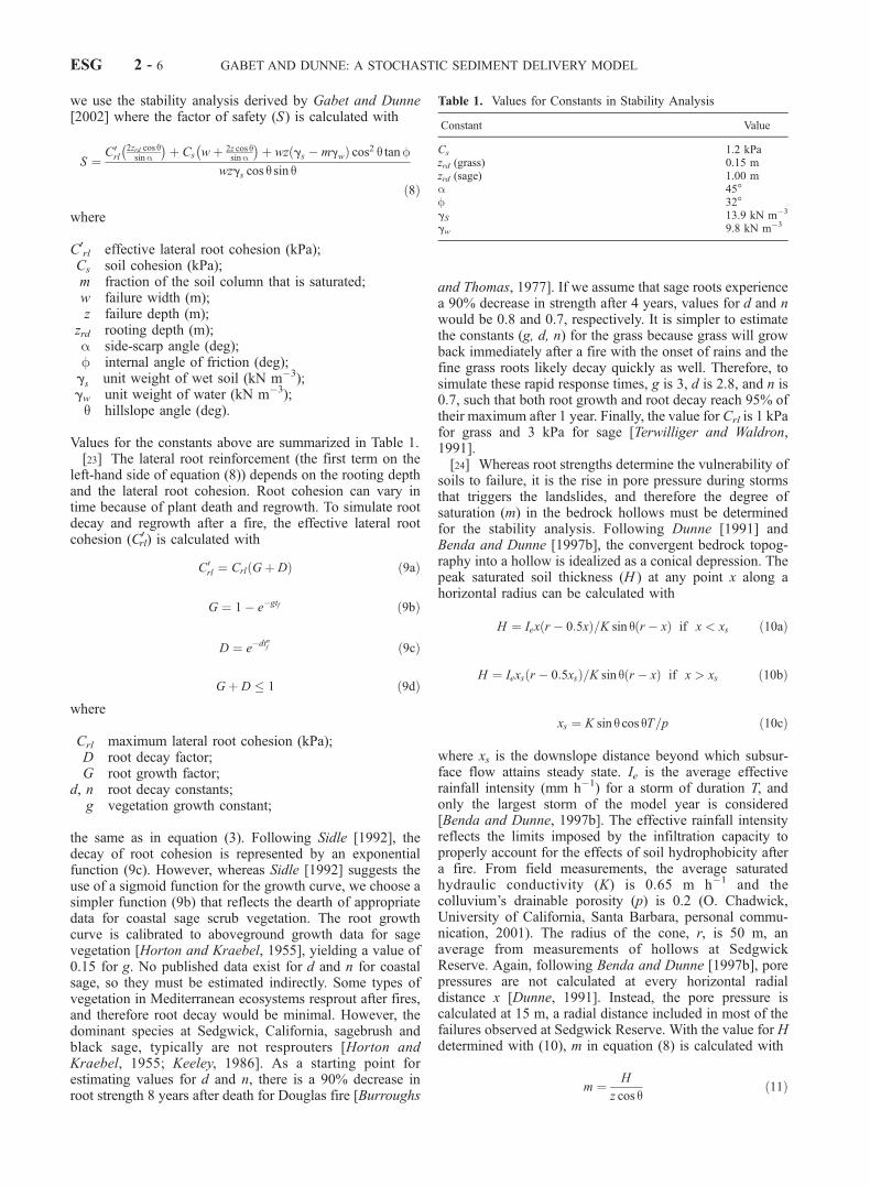
Values for the constants above are summarized in Table 1.[23] The lateral root reinforcement (the first term on the

left-hand side of equation (8)) depends on the rooting depthand the lateral root cohesion. Root cohesion can vary intime because of plant death and regrowth. To simulate rootdecay and regrowth after a fire, the effective lateral rootcohesion (C0

rl) is calculated with

C0rl ¼ Crl Gþ Dð Þ ð9aÞ

G ¼ 1� e�gtf ð9bÞ

D ¼ e�dtn

f ð9cÞ

Gþ D � 1 ð9dÞ

where

Crl maximum lateral root cohesion (kPa);D root decay factor;G root growth factor;

d, n root decay constants;g vegetation growth constant;

the same as in equation (3). Following Sidle [1992], thedecay of root cohesion is represented by an exponentialfunction (9c). However, whereas Sidle [1992] suggests theuse of a sigmoid function for the growth curve, we choose asimpler function (9b) that reflects the dearth of appropriatedata for coastal sage scrub vegetation. The root growthcurve is calibrated to aboveground growth data for sagevegetation [Horton and Kraebel, 1955], yielding a value of0.15 for g. No published data exist for d and n for coastalsage, so they must be estimated indirectly. Some types ofvegetation in Mediterranean ecosystems resprout after fires,and therefore root decay would be minimal. However, thedominant species at Sedgwick, California, sagebrush andblack sage, typically are not resprouters [Horton andKraebel, 1955; Keeley, 1986]. As a starting point forestimating values for d and n, there is a 90% decrease inroot strength 8 years after death for Douglas fire [Burroughs

and Thomas, 1977]. If we assume that sage roots experiencea 90% decrease in strength after 4 years, values for d and nwould be 0.8 and 0.7, respectively. It is simpler to estimatethe constants (g, d, n) for the grass because grass will growback immediately after a fire with the onset of rains and thefine grass roots likely decay quickly as well. Therefore, tosimulate these rapid response times, g is 3, d is 2.8, and n is0.7, such that both root growth and root decay reach 95% oftheir maximum after 1 year. Finally, the value for Crl is 1 kPafor grass and 3 kPa for sage [Terwilliger and Waldron,1991].[24] Whereas root strengths determine the vulnerability of

soils to failure, it is the rise in pore pressure during stormsthat triggers the landslides, and therefore the degree ofsaturation (m) in the bedrock hollows must be determinedfor the stability analysis. Following Dunne [1991] andBenda and Dunne [1997b], the convergent bedrock topog-raphy into a hollow is idealized as a conical depression. Thepeak saturated soil thickness (H ) at any point x along ahorizontal radius can be calculated with

H ¼ Iex r � 0:5xð Þ=K sin qðr � xÞ if x < xs ð10aÞ

H ¼ Iexs r � 0:5xsð Þ=K sin qðr � xÞ if x > xs ð10bÞ

xs ¼ K sin q cos qT=p ð10cÞ

where xs is the downslope distance beyond which subsur-face flow attains steady state. Ie is the average effectiverainfall intensity (mm h�1) for a storm of duration T, andonly the largest storm of the model year is considered[Benda and Dunne, 1997b]. The effective rainfall intensityreflects the limits imposed by the infiltration capacity toproperly account for the effects of soil hydrophobicity aftera fire. From field measurements, the average saturatedhydraulic conductivity (K) is 0.65 m h�1 and thecolluvium’s drainable porosity (p) is 0.2 (O. Chadwick,University of California, Santa Barbara, personal commu-nication, 2001). The radius of the cone, r, is 50 m, anaverage from measurements of hollows at SedgwickReserve. Again, following Benda and Dunne [1997b], porepressures are not calculated at every horizontal radialdistance x [Dunne, 1991]. Instead, the pore pressure iscalculated at 15 m, a radial distance included in most of thefailures observed at Sedgwick Reserve. With the value for Hdetermined with (10), m in equation (8) is calculated with

m ¼ H

z cos qð11Þ

Table 1. Values for Constants in Stability Analysis

Constant Value

Cs 1.2 kPazrd (grass) 0.15 mzrd (sage) 1.00 ma 45�f 32�gS 13.9 kN m�3

gw 9.8 kN m�3

ESG 2 - 6 GABET AND DUNNE: A STOCHASTIC SEDIMENT DELIVERY MODEL

[25] Surveys of the failures at Sedgwick Reserve revealeda systematic decline in failure width with increasing slope inthe sage [Gabet and Dunne, 2002]. From the data presentedby Gabet and Dunne [2002], failure width in equation (8) iscalculated as a function of slope with

w ¼ 12ðq� 31Þ�0:5 ð12Þ

For slopes less than 32�, failure widths are set at 13 m.Because there was no apparent relationship between failurewidth and slope in the grasslands, the average width forgrassland failures (5 m) is used [Gabet and Dunne, 2002].Failure volumes are determined as the product of the width,the soil depth at failure, and the failure length calculatedfrom the average length/width ratio (2.7) [Gabet andDunne, 2002].

2.6. Hollow Filling

[26] After a bedrock hollow is evacuated, the landslidescar is refilled by sediment transported from adjacent slopesby soil creep. The net volume (V) of sediment coming intothe hollow per meter length of scar (l) can be calculated as afunction of time since the previous landslide (tl) with

V tlð Þl

¼ 2qstl sinlrs

ð13Þ

where rs is the dry bulk density of the soil and l is theconvergence angle into the hollow [Reneau and Dietrich,1991]. Landslide scars are represented as troughs with side-scarps at an angle a [Gabet and Dunne, 2002] such that thesoil depth in each hollow (z) can be expressed as a functionof time since the previous landslide with [Benda andDunne, 1997b]:

z tlð Þ ¼ w2 þ 4V tlð Þ cota� �0:5�wh i tana

2ð14Þ

Average values from Sedgwick Reserve for rS and l are1190 kg m�3 and 32�, respectively.2.7. Postfire Transport Processes

[27] In addition to background dry ravel, there is a formof dry ravel associated with fire. In steep semiarid environ-ments with shrubby vegetation, transport by dry ravel aftera fire can be extensive, as sediment that has accumulatedbehind litter and vegetation is released when the vegetationis burned [Wells, 1987; Florsheim et al., 1991]. Fromsediment traps installed in coastal sage scrub in anticipationof a prescribed fire near Sedgwick Reserve, the specificflux of sediment from postfire dry ravel can be determinedwith equation (6) with a value of 0.03 kg m�1 fire�1 for kand 1.01 for m. The amount of postfire dry ravel reportedhere is less than what has been observed elsewhere. Forexample, Wells [1987] observed that small channels in theSan Dimas Experimental Forest, near Los Angeles, werecompletely filled with dry ravel deposits immediately aftera fire in shrubby vegetation. Davis et al. [1989] found that0.20 m3 of dry ravel deposits were delivered per meter lengthof channel in the month following a chaparral fire nearSanta Barbara. Assuming a bulk density of 1300 kg m�3 forthe deposit and assuming that the deposits accumulatedfrom both sides of the channel, the specific mass flux was

then 130 kg m�1. This is significantly more than what wasobserved near Sedgwick Reserve; for example, equation (6)parameterized with the values for k and m above predicts aspecific mass flux of 0.20 kg m�1. A difference in lithologyis the most likely explanation for the discordance betweenthe rates of postfire dry ravel at Sedgwick Reserve andthose reported by Davis et al. [1989]. The watershed studiedby Davis et al. [1989] is underlain by shale and sandstoneand the clasts in the postfire dry ravel deposits were wellsorted, with an average size of 4 mm [Florsheim et al.,1991]. In contrast, the fanglomerate at Sedgwick Reserveweathers into particle sizes that range from clay to gravel.A greater variance in particle size will decrease the fluxby increasing the effective roughness of the surface [Kirkbyand Statham, 1974]. Additionally, the soils at SedgwickReserve are generally high in smectitic clays [Shipman,1972], and the cohesion from these clays may inhibitraveling.[28] Along with dry ravel, thin debris flows (TDFs) are

also limited to the coastal sage scrub. Gabet [2003a] hasdeveloped a numerical model for TDFs that couples sub-surface flow routing through the top 1–2 cm of soil with aninfinite-slope stability analysis. The TDF model predicts thelocation and timing of these shallow failures during rain-storms such that the mass of sediment transported across aunit contour width of slope by TDF may be determined with[Gabet, 2003a]

mass

unit width¼ ALztrst ð15Þ

whereA fraction of area covered by TDF scars;L length of TDF scar (m);zt failure depth (m);rst bulk density of the top layer of soil (kg m�3).L is determined with the model described above; from fieldobservations, d is 1.5 cm and A is 0.60 [Gabet, 2003a]. Thebulk density of the upper layer of soil, adjusted for organiccontent, is 560 kg m�3 [Gabet, 2003a].[29] Many simulation runs of the TDF model described

by Gabet [2003a] were done to determine the excess rainfall(i.e., i � f ) thresholds necessary for triggering TDFs atvarious slope angles. These runs indicated that only about0.3 cm of rain will cause TDFs, which agrees well withWells [1987]. In the larger model presented here, when therainfall threshold is reached, the sediment delivered to thebase of the hillslope is determined with equation (15).

2.8. Model Operation

[30] The algorithm for the model is shown in Figure 6.The climate parameters, mean rainfall intensity, mean stormduration, mean fire size, and fire recurrence interval arespecified at the beginning of each run and can be changed atany time during the run. Similarly, vegetation type, whichdetermines the suite of relevant transport processes, isspecified for each hillslope strip at the start of the modelsimulation and can be changed at any time. The initial soildepth in each bedrock hollow is determined by randomlyassigning a value for tl, the time since the last landslide (seeequations (13) and (14)). Values for tl are normally distrib-uted with a mean of 100 years such that initial soil depthsare less than 0.20 m. Because slope angles and soil depths

GABET AND DUNNE: A STOCHASTIC SEDIMENT DELIVERY MODEL ESG 2 - 7

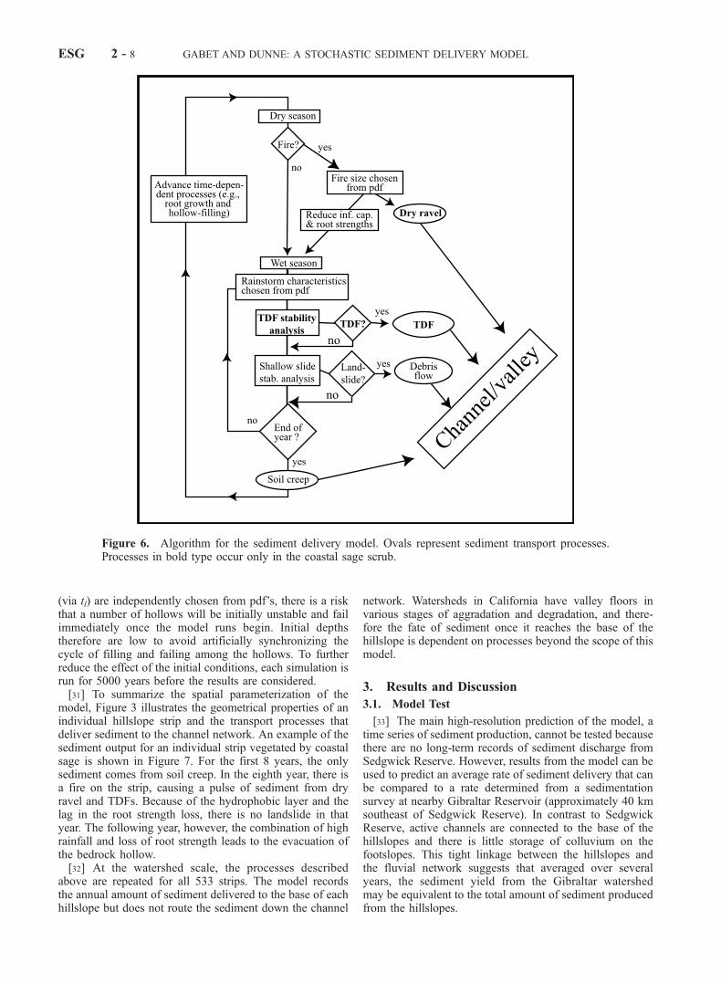
(via tl) are independently chosen from pdf’s, there is a riskthat a number of hollows will be initially unstable and failimmediately once the model runs begin. Initial depthstherefore are low to avoid artificially synchronizing thecycle of filling and failing among the hollows. To furtherreduce the effect of the initial conditions, each simulation isrun for 5000 years before the results are considered.[31] To summarize the spatial parameterization of the

model, Figure 3 illustrates the geometrical properties of anindividual hillslope strip and the transport processes thatdeliver sediment to the channel network. An example of thesediment output for an individual strip vegetated by coastalsage is shown in Figure 7. For the first 8 years, the onlysediment comes from soil creep. In the eighth year, there isa fire on the strip, causing a pulse of sediment from dryravel and TDFs. Because of the hydrophobic layer and thelag in the root strength loss, there is no landslide in thatyear. The following year, however, the combination of highrainfall and loss of root strength leads to the evacuation ofthe bedrock hollow.[32] At the watershed scale, the processes described

above are repeated for all 533 strips. The model recordsthe annual amount of sediment delivered to the base of eachhillslope but does not route the sediment down the channel

network. Watersheds in California have valley floors invarious stages of aggradation and degradation, and there-fore the fate of sediment once it reaches the base of thehillslope is dependent on processes beyond the scope of thismodel.

3. Results and Discussion

3.1. Model Test

[33] The main high-resolution prediction of the model, atime series of sediment production, cannot be tested becausethere are no long-term records of sediment discharge fromSedgwick Reserve. However, results from the model can beused to predict an average rate of sediment delivery that canbe compared to a rate determined from a sedimentationsurvey at nearby Gibraltar Reservoir (approximately 40 kmsoutheast of Sedgwick Reserve). In contrast to SedgwickReserve, active channels are connected to the base of thehillslopes and there is little storage of colluvium on thefootslopes. This tight linkage between the hillslopes andthe fluvial network suggests that averaged over severalyears, the sediment yield from the Gibraltar watershedmay be equivalent to the total amount of sediment producedfrom the hillslopes.

Figure 6. Algorithm for the sediment delivery model. Ovals represent sediment transport processes.Processes in bold type occur only in the coastal sage scrub.

ESG 2 - 8 GABET AND DUNNE: A STOCHASTIC SEDIMENT DELIVERY MODEL

[34] The watershed upstream of the Gibraltar Reservoir issteeper than the one modeled at Sedgwick Reserve so thetopographic attributes must be redefined. From an analysisof the USGS Little Pine Mountain quadrangle, the averagehillslope length is approximately 110 m and the averageslope angle is 36�. With these hillslope parameters and acoastal sage scrub vegetation cover, the model predicts anaverage sediment yield of 128 t km�2 yr�1. Data from theSanta Barbara County Water Agency (SBCWA) indicatethat averaged over 25 years, the volumetric sediment yieldfrom the Gibraltar Reservoir watershed is approximately640 m3 km�2 yr�1. Although the bulk density of the sedimenthas not been measured (K. Goodenough, SBCWA, personalcommunication, 2001), bulk densities for fine-grainedreservoir deposits may vary from 370 to 530 kg m�3

[Meade, 1966]. With these values, the mass sediment yieldinto Gibraltar Reservoir is 250–360 t km�2 yr�1.[35] The predicted rate is 25% less than the lowest rate

estimated from the reservoir data. It is possible that we haveoverlooked an important transport process; however, thedifference between the model results and the calculatedsediment yield is likely to due to an underprediction inthe rates of dry ravel. As previously noted, the soils atSedgwick Reserve do not appear to be as susceptible to dryravel as coarser soils. In contrast, the lithology of theGibraltar Reservoir watershed is dominated by shales andsandstones, similar to the bedrock that produced the highrates of postfire dry ravel measured by Davis et al. [1989].

To approximately match Davis et al.’s [1989] data, thevalue of k is increased to 33 kg m�1 fire�1 in equation (5).Additionally, data reported by Anderson et al. [1959] andKrammes [1965] from the San Gabriel Mountains insouthern California may be used to estimate a value of2.5 kg m�1 yr�1 for background dry ravel. The San GabrielMountains are granitic, producing sand-sized weatheredmaterial [Anderson et al., 1959], similar to the regolith inthe Gibraltar watershed. With these new values, the pre-dicted yield becomes 346 t km�2 yr�1, suggesting that themodel is capturing the essence of sediment delivery in thistype of landscape. Ideally, we would have used a detailedfire and precipitation record from the Gibraltar watershed todrive the model; unfortunately none exist. However, thewatershed may be large enough (520 km2) that it mayintegrate the range of climatic events represented in themodel run. Additionally, surveys from other reservoirs inthe region (Juncal, Twitchell, and Bradbury) record sedi-ment yields similar to the Gibraltar watershed (SBCWA).

3.2. Vegetation Change at Sedgwick Reserve

[36] As previously noted, human-induced vegetation con-version from native scrub to exotic grasses is a commonpractice in the region. Additionally, coupled climate-vege-tation models predict that in the next 100 years, grassysavanna communities may replace shrublands throughoutthe Coast Ranges of California [Field et al., 1999]. Toinvestigate the effects of vegetation change on sedimentdelivery, the model was run under sage for 10,000 years andthen run under grasslands for another 10,000 years. Tenthousand years was chosen because the model runs must belong enough such that differences resulting from changes inthe model parameters can be distinguished from variationscaused by the stochastic forcing.[37] From Figures 8 and 9, there are noticeable differ-

ences in sediment delivery between the sage and the grass-lands. In the coastal sage scrub, there is greater interannualvariability in annual sediment delivery, whereas in thegrasslands, sediment delivery events are relatively muted.Figure 9 also shows that the rate of soil creep is approxi-mately 4 times greater in the grasslands than in the coastalsage. Average rates of annual sediment delivery and spa-tially averaged soil erosion rates for both vegetation typesare listed in Table 2. These results suggest that sedimentdelivery is 38% higher under grassland than coastal sage.[38] The primary reason for the marked difference in the

nature of sediment delivery between the two vegetationcovers is attributable to the difference in relevant transportprocesses. The relative magnitudes of the different pro-cesses are compared in Figure 10. In the sage, 70% of thetotal sediment delivered is by catastrophic processes: TDFsand landslides. This indicates that sediment delivery in thesage is strongly linked to the occurrence of fires. Incontrast, soil creep accounts for 72% of the sedimentproduction in the grasslands. Because of the absence ofTDFs in the grasslands, sediment production is not assensitive to fires. Therefore vegetation conversion changesnot only the magnitude of sediment supply but also thenature of sediment delivery from catastrophic to chronic.Finally, the relatively weak contribution of grass roots tooverall soil strength, as well as its rapid regrowth after afire, decouples the occurrence of landslides from the fireregime.

Figure 7. Illustration of the sediment delivery from onehillslope strip with sage vegetation. The top panel is theannual rainfall with a fire in the eighth year indicated by anasterisk. The second panel is the sediment flux from dryravel and includes both the background rate and the pulse ofdry ravel after a fire. The third panel represents the sedimentdelivered from TDFs during rainstorms after the fire. Thebottom panel is the delivery of sediment from a shallowlandslide.

GABET AND DUNNE: A STOCHASTIC SEDIMENT DELIVERY MODEL ESG 2 - 9

[39] Results from the model also suggest that the grass-land hollows will fail more often than coastal sage hollows(Table 2). In the grasslands, the bedrock hollows fill upmore rapidly because of higher rates of soil creep and theyfail with thinner soil depths because of the weaker rootreinforcement. Additionally, the predicted spike in landslid-ing frequency soon after vegetation conversion (at 10,000years in Figure 11) is a phenomenon commonly observed

throughout the region [Corbett and Rice, 1966; Bailey andRice, 1969; Rice et al., 1969; Rice and Foggin, 1971;Terwilliger and Waldron, 1991; Gabet and Dunne, 2002].This transient increase in landsliding is likely due to atemporary disequilibrium between the prevailing root rein-forcement and soil depths [Rice and Foggin, 1971; Gabetand Dunne, 2002]. Gabet and Dunne [2002] have demon-strated that an abrupt decrease in root reinforcement causedby vegetation conversion increases the likelihood of shallowlandsliding on hillslopes that were previously stable.

3.3. Climate Change at Sedgwick Reserve

[40] Given the importance of climate for sediment deliv-ery, it is valuable to consider how global climate change mayalter the nature of sediment production. A recently publishedreport has described several potential consequences ofglobal warming in California [Field et al., 1999]. On thebasis of general circulation models, the report foresees anincrease in winter rains followed by drier summers due toincreases in dry, offshore winds (Santa Ana winds). Driersummers would likely increase the frequency and intensityof wildfires throughout the state, particularly in southernCalifornia [Field et al., 1999]. Giorgi et al. [1994]predicted an approximately 30% increase in winter rainfalland a 4�C rise in summer temperatures in California with adoubling of atmospheric CO2. Given these estimates,Davis and Michaelsen [1995] used an explicit fire ignition

Figure 8. Predicted annual sediment delivery with vegeta-tion conversion. The first 10,000 years are with sagevegetation and the last 10,000 years with grass. The amountof sediment delivered each year in the sage has a higherinterannual variability than in the grasslands (note that themaximum sediment delivery occurs in the coastal sage eachtime the entire model domain burns). In the grasslands, thesediment pulses are significantly attenuated relative to thecoastal sage scrub.

Figure 9. The 600 years bracketing the vegetationconversion. The differences in the magnitude of sedimentdelivery events between vegetation types are apparent. Theflux from soil creep, the baseline sediment delivery, isgreater in the grasslands than in the sage, accounting for thehigher average rates of sediment loading. Note thesemilogarithmic scale.

Table 2. Average Predicted Rates of Sediment Production, Rates

of Soil Erosion, and Landslide Frequencya

Production,t km�2 yr�1

Erosion,mm kyr�1

Landslides,slides km�2 yr�1

Present climateSage scrub 71 60 0.58Grassland 98 82 1.28

2 � CO2

Sage scrub 80 68 0.61Grassland 100 84 1.55

aAll differences between vegetation types and climates are statisticallysignificant ( p < 0.005). The predicted increase in ‘‘2 � CO2’’ climatescenario is based on results from Giorgio et al. [1994] and Davis andMichaelsen [1995].

Figure 10. (a) Relative proportions of sediment contrib-uted by each transport process in the sage scrub. Themajority of sediment is delivered episodically by TDFs andlandslides. (b) Proportions of sediment contributed by eachprocess in the grasslands. The majority of sediment isdelivered by soil creep, indicating that sediment delivery inthe grasslands tends to occur as a steady trickle rather thanas large, infrequent pulses.

ESG 2 - 10 GABET AND DUNNE: A STOCHASTIC SEDIMENT DELIVERY MODEL

and propagation model to forecast a 17% decrease in thefire recurrence interval in central coastal California.[41] The model presented here can be used to examine the

effects of the predicted changes in the rainfall and fireregimes. First, the annual distribution of rainfall (Figure 4)is shifted to increase the average annual rainfall by 30%, from50 to 65 cm yr�1. Increased annual rainfall may be accom-modated by a rise in the number of storms, storm duration, orrainfall intensity. Climate models suggest that rainfall maybecome more intense [Houghton et al., 1992] so the averagerainfall intensity is increased from 0.18 to 0.23 cm h�1.Second, to account for the change in the fire recurrenceinterval, the base ignition probability in equation (3) isadjusted to produce a fire recurrence interval of 67 years,instead of 81 years. However, the effect of climate change onthe fire recurrence interval is likely more complicated thanthe simple adjustment made here because the present recur-rence interval is largely due to regional fire suppression[Keeley et al., 1999].[42] The results (Table 2) indicate that climate change

will increase the sediment delivery from coastal sage hill-slopes by 10% but will only increase the delivery fromgrassland hillslopes by 2%. This difference would beexpected since the sediment delivery processes on sagehillslopes are more sensitive to fires. In both types ofvegetation, however, the frequency of landsliding increasesdue to the more frequent fires that reduce root reinforcementand the larger storms. The increase in storm intensitydirectly affects the landslide stability analysis throughequations (8), (10), and (11) such that the hollows reach acritical saturation more often. The increase in landslidefrequency implies that failure volumes will be smaller andthat average soil depths in the hollows will decrease [Gabetand Dunne, 2002].[43] On coastal sage hillslopes, the modeled increase in

sediment production due to vegetation conversion is nearly4 times greater than the increase due to climate change. Thisresult leads to the interesting speculation that climaticchanges, expressed as purely meteorological phenomena,may only have a minimal impact on changes in sedimentproduction. In contrast, changes in vegetation community

driven by regional climate change may have much greaterconsequences.

4. Conclusion

[44] Sediment loading to channels affects a range ofconcerns, including debris flow hazards, water quality,and reservoir sedimentation. In this contribution, we presenta computer model that drives field-based hillslope sedimenttransport equations with stochastically generated rainstormsand fires. The model is used to examine how land manage-ment strategies and climate change may alter both the ratesand the processes of sediment delivery. The results suggestthat conversion of coastal sage scrub to grassland, acommon practice, increases sediment delivery by approxi-mately 38% but that the sediment delivery regime switchesfrom being dominated by catastrophic processes (e.g., thindebris flows) to being dominated by chronic soil creepprocesses. The results from the model also suggest thatchanges in vegetation engendered by changes in climatewill increase sediment production more than changes in theclimatic events themselves.

[66] Acknowledgments. We thank M. Williams, R. Skillins, andV. Boucher of Sedgwick Reserve for their enthusiastic help in facilitatingthe fieldwork. We are grateful for the help that C. Marcinkovich generouslyprovided in the coding of the model, and we thank the reviewers for theirinsightful comments. Supplies and salary for E. Gabet were supported byU.C. Water Resources grant UCAL-W-917, NSF-SGER DEB9813669, aSigma Xi grant, and a Mildred Mathias grant.

ReferencesAnderson, H. W., G. B. Coleman, and P. J. Zinke, Summer slides andwinter scour, dry-wet erosion in Southern California mountains, U.S.For. Serv. Pac. Southwest For. Range Exp. Stn. Tech. Pap., PSW-36,PSW-36, 1959.

Bailey, R. G., and R. M. Rice, Soil slippage: An indicator of slope instabil-ity on chaparral watersheds of southern California, Prof. Geogr., 21(3),172–177, 1969.

Benda, L., and T. Dunne, Stochastic forcing of sediment routing and storagein channel networks, Water Resour. Res., 33, 2849–2863, 1997a.

Benda, L., and T. Dunne, Stochastic forcing of sediment supply to channelnetworks from landsliding and debris flow, Water Resour. Res., 33,2865–2880, 1997b.

Beven, K., Towards the use of catchment geomorphology in flood fre-quency predictions, Earth Surf. Processes Landforms, 12, 69–82, 1987.

Burroughs, E. R., and B. R. Thomas, Declining root strength in Douglas-firafter felling as a factor in slope stability, USDA For. Serv. Res. Pap.,INT-190, 1977.

Campbell, R. H., Soil slips, debris flows, and rainstorms in the SantaMonica Mountains and vicinity, southern California, U.S. Geol. Surv.Prof., 851, 1975.

Cerda, A., Changes in overland flow and infiltration after a rangeland fire ina Mediterranean scrubland, Hydrol. Processes, 12, 1031–1042, 1998.

Corbett, E. S., and R. M. Rice, Soil slippage increased by brush conversion,U.S. For. Serv. Pac. Southwest For. Range Exp. Stn. Res. Note, PSW-128,1–8, 1966.

Davis, F. W., and D. A. Burrows, Modeling fire regime in Mediterraneanlandscapes, in Patch Dynamics, edited by S. Levin, T. Powell, andJ. Steele, pp. 247–259, Springer-Verlag, New York, 1993.

Davis, F. W., and J. Michaelsen, Sensitivity of fire regime in chaparralecosystems to climate change, in Global Change and Mediterranean-Type Ecosystems, edited by J. M. Moreno and W. C. Oechel, pp. 435–456, Springer-Verlag, New York, 1995.

Davis, F. W., E. A. Keller, A. Parikh, and J. Florsheim, Recovery of thechaparral riparian zone after wildfire, USDA For. Serv. Gen. Tech. Rep.PSW-110, 194–203, 1989.

DeBano, L. F., Water repellent soils: A state of the art, USDA For. Serv.Res. Pap., PSW-46, 1–21, 1981.

Denny, C., and J. Goodlett, Microrelief resulting from fallen trees, U.S.Geol. Surv. Prof. Publ., 288, 59–68, 1956.

Figure 11. Changes in landslide frequency with vegeta-tion conversion at 10,000 years. Because of the faster ratesof hollow-filling and the weaker root reinforcement,landslides occur more frequently in the grasslands. Thespike in landslide frequency immediately after the vegeta-tion conversion is a commonly observed phenomenonthroughout Mediterranean landscapes and is due to a suddendisequilibrium between soil depths and root reinforcement.

GABET AND DUNNE: A STOCHASTIC SEDIMENT DELIVERY MODEL ESG 2 - 11

Dibblee, T. W. J., Geologic map of the Los Olivos Quadrangle,Map DF-44,Dibblee Geol. Found., Santa Barbara, Calif., 1993.

Dietrich, W. E., and T. Dunne, Sediment budget for a small catchment inmountainous terrain, Z. Geomorphol. Suppl., 29, 191–206, 1978.

Dunne, T., Stochastic aspects of the relations between climate, hydrology andlandform evolution, Trans. Jpn. Geomorphol. Union, 12(1), 1–24, 1991.

Eagleson, P. S., Dynamics of flood frequency, Water Resour. Res., 8(4),878–898, 1972.

Field, C. B., et al., Confronting climate change in California: Ecologicalimpacts on the Golden State, Union of Concerned Sci. and the Ecol. Soc.of Am., Washington, D. C., 1999.

Fierer, N. G., and E. G. Gabet, Transport of carbon and nitrogen bysurface runoff from hillslopes in the Central Coast region of California,J. Environ. Qual., 31, 1207–1213, 2002.

Florsheim, J. L., E. A. Keller, and D. W. Best, Fluvial sediment transport inresponse to moderate storm flows following chaparral wildfire, VenturaCounty, southern California, Geol. Soc. Am. Bull., 103, 504–511, 1991.

Gabet, E. J., Gopher bioturbation: Field evidence for nonlinear hillslopediffusion, Earth Surf. Processes Landforms, 25(13), 1419–1428, 2000.

Gabet, E. J., Post-fire thin debris flows: Field observations of sedimenttransport and numerical modeling, Earth Surf. Processes Landforms, inpress, 2003a.

Gabet, E. J., Sediment transport by dry ravel, J. Geophys. Res., 108(B1),2049, doi:10.1029/2001JB001686, 2003b.

Gabet, E. J., and T. Dunne, Landslides on coastal sage-scrub and grasslandhillslopes in a severe El Nino winter: The effects of vegetation conver-sion on sediment delivery, Geol. Soc. Am. Bull., 114(8), 983–990, 2002.

Gabet, E. J., and T. Dunne, Sediment detachment by rainpower, WaterResour. Res., 39(1), 1002, doi:10.1029/2001WR000656, 2003.

Gabet, E. J., O. J. Reichman, and E. Seabloom, The effects of bioturbationon soil processes and sediment transport, Annu. Rev. Earth Planet. Sci.,31, 259–273, 2003.

Giorgi, F., F. S. Brodeur, and G. T. Bates, Regional climate change scenar-ios over the United States produced with a nested regional climate model,J. Clim., 7(3), 375–399, 1994.

Hibbert, A. R., Increases in streamflow after converting chaparral to grass,Water Resour. Res., 7(1), 71–80, 1971.

Horton, J. S., and C. J. Kraebel, Development of vegetation after fire in thechamise chaparral of southern California, Ecology, 36(2), 244–262, 1955.

Houghton, J., B. Callander, and S. Varney (Eds.), Climate change 1992:The supplementary report to the IPCC scientific assessment, 199 pp.,Cambridge Univ. Press, New York, 1992.

Iida, T., A stochastic hydro-geomorphological model for shallow landslid-ing due to rainstorm, Catena, 34, 293–313, 1999.

Keeley, J. A., Resilience of Mediterranean shrub communities to fires,Ecology, 45, 243–245, 1986.

Keeley, J. E., C. J. Fotheringham, and M. Morais, Reexamining firesuppression impacts on brushland fire regimes, Science, 284, 1829–1832, 1999.

Kennett, J. P., and B. L. Ingram, A 20,000-year record of ocean circulationand climate change from the Santa Barbara basin, Nature, 377, 510–514,1995.

Kirkby, M. J., Hydrological slope models: The influence of climate, inGeomorphology and Climate, edited by E. Derbyshire, pp. 247–268,John Wiley, Hoboken, N. J., 1976.

Kirkby, M. J., and I. Statham, Surface stone movement and scree formation,J. Geol., 83, 349–362, 1974.

Krammes, J. S., Seasonal debris movement from steep mountainside slopesin southern California, in Proceedings of the Federal Inter-Agency Sedi-mentation Conference, U.S. Dep. of Agric. Misc. Publ. 970, 85–88,1965.

Meade, R. H., Factors influencing the early stages of the compaction ofclays and sands—Review, J. Sediment. Petrol., 36(4), 1085–1101, 1966.

Reistenberg, M. M., and S. Sovonick-Dunford, The role of woody vegeta-tion in stabilizing slopes in the Cincinnati area, Ohio, Geol. Soc. Am.Bull., 94, 506–518, 1983.

Reneau, S. L., and W. E. Dietrich, Erosion rates in the southern OregonCoast Range: Evidence for an equilibrium between hillslope erosionand sediment yield, Earth Surf. Processes Landforms, 16, 307–322,1991.

Rice, R. M., Sedimentation in the chaparral: How do you handle unusualevents?, in Sediment Budgets and Routing in Forested Drainage Basins,edited by F. J. Swanson et al., pp. 39–49, U.S. Dep. of Agric. For. Serv.,1982.

Rice, R. M., and G. T. Foggin, Effect of high intensity storms on soilslippage on mountainous watersheds in southern California, WaterResour. Res., 7(6), 1485–1496, 1971.

Rice, R. M., E. S. Corbett, and R. G. Bailey, Soil slips related to vegetation,topography, and soil in southern California, Water Resour. Res., 5(3),647–659, 1969.

Selby, M. J., Hillslope Materials and Processes, Oxford Univ. Press, NewYork, 1993.

Shipman, G. E., Soil Survey of Northern Santa Barbara Area, California,U.S. Dep. of Agric. Soil Conserv. Serv., Washington, D. C., 1972.

Sidle, R. C., A theoretical model of the effects of timber harvesting on slopestability, Water Resour. Res., 28(7), 1897–1910, 1992.

Sklar, L., and W. E. Dietrich, River longitudinal profiles and bedrockincision models: Stream power and the influence of sediment supply,in Rivers Over Rock: Fluvial Processes in Bedrock Channels, Geophys.Monogr. Ser., vol. 107, edited by K. J. Tinkler and E. E. Wohl, pp. 237–260, AGU, Washington, D. C., 1998.

Terwilliger, V. J., and L. J. Waldron, Effects of root reinforcement on soil-slip patterns in the Transverse Ranges of southern California, Geol. Soc.Am. Bull., 103, 775–785, 1991.

Tucker, G. E., and R. L. Bras, A stochastic approach to modeling the role ofrainfall variability in drainage basin evolution, Water Resour. Res., 36(7),1953–1964, 2000

Wagner, C. E. V., Age-class distribution and the forest fire cycle, Can.J. For. Res., 8, 220–227, 1978.

Wells, W. G., The effects of fire on the generation of debris flows in south-ern California, Rev. Eng. Geol., 7, 105–114, 1987.

����������������������������T. Dunne, Donald Bren School of Environmental Science and Manage-

ment and Department of Geological Sciences, University of California,Santa Barbara, Santa Barbara, CA 93106, USA.

E. J. Gabet, Department of Geology, University of Montana, Missoula,MT 59812, USA. (manny.gabet@mso.umt.edu)

ESG 2 - 12 GABET AND DUNNE: A STOCHASTIC SEDIMENT DELIVERY MODEL